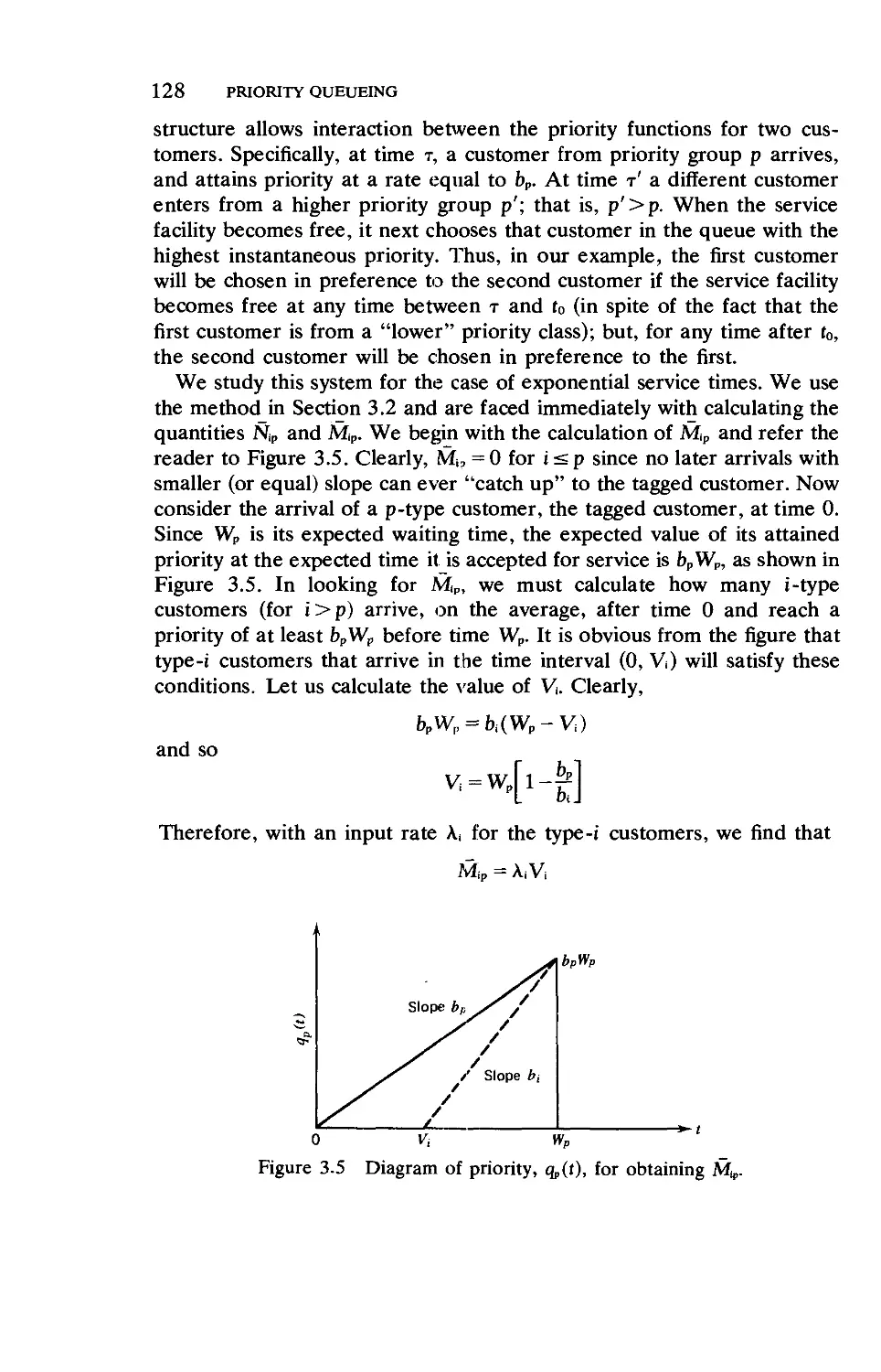
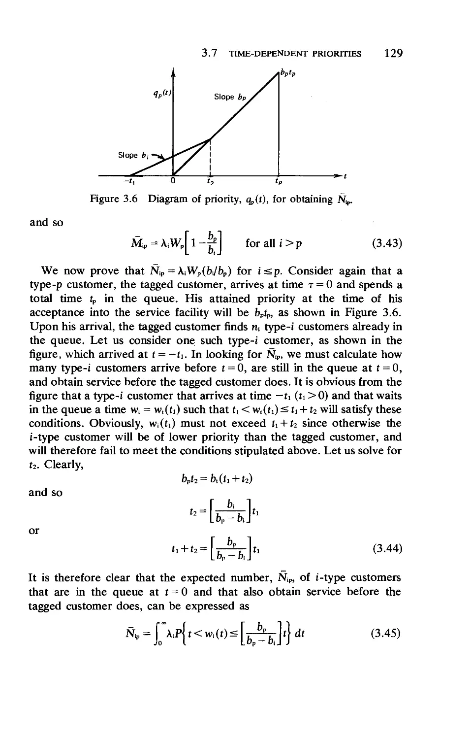
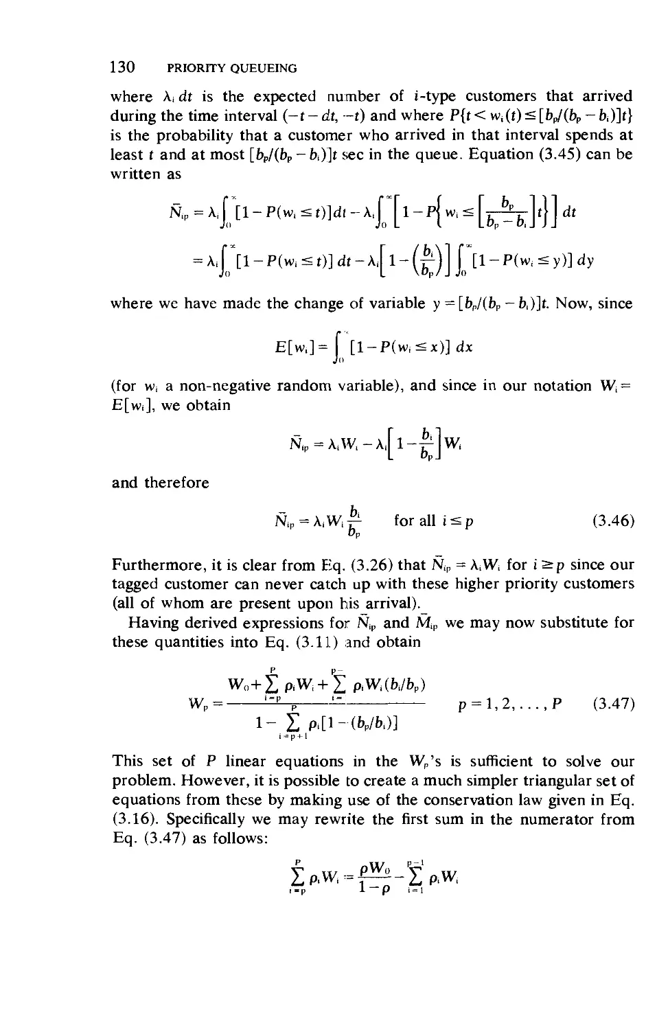
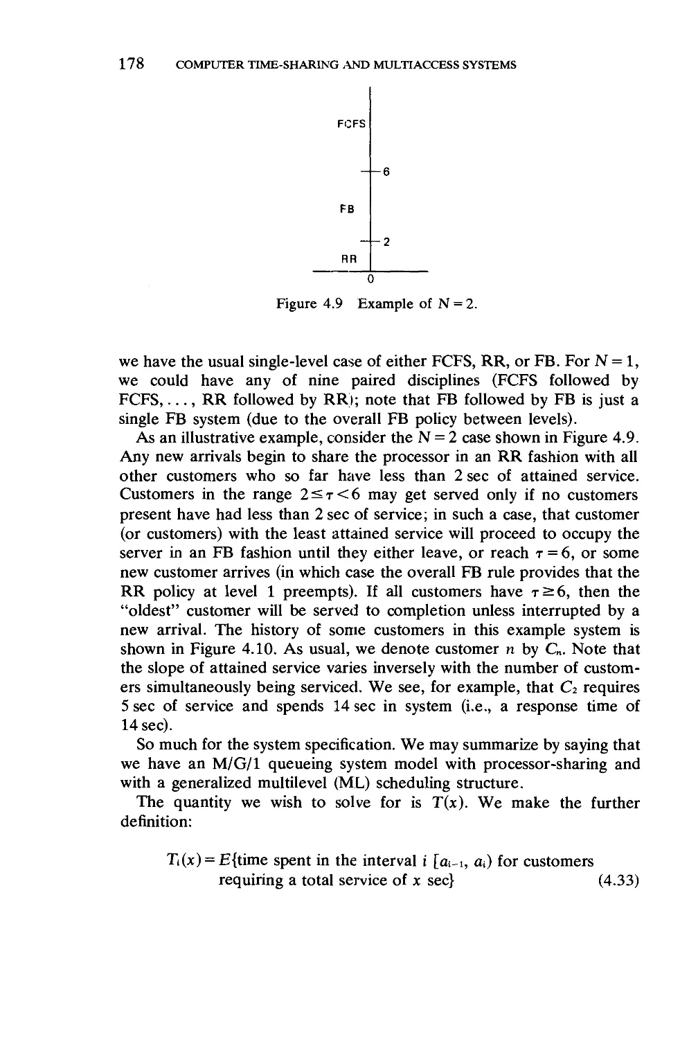
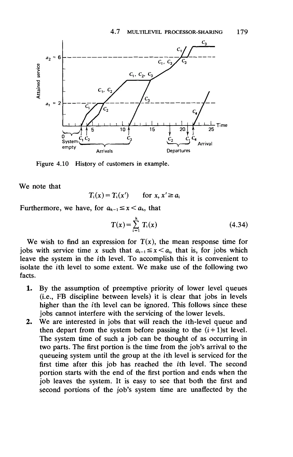
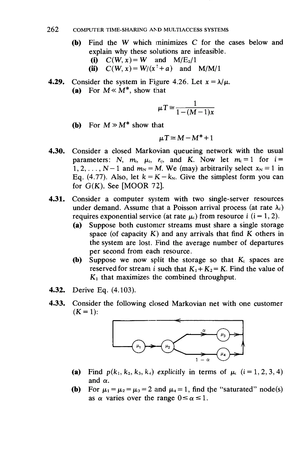
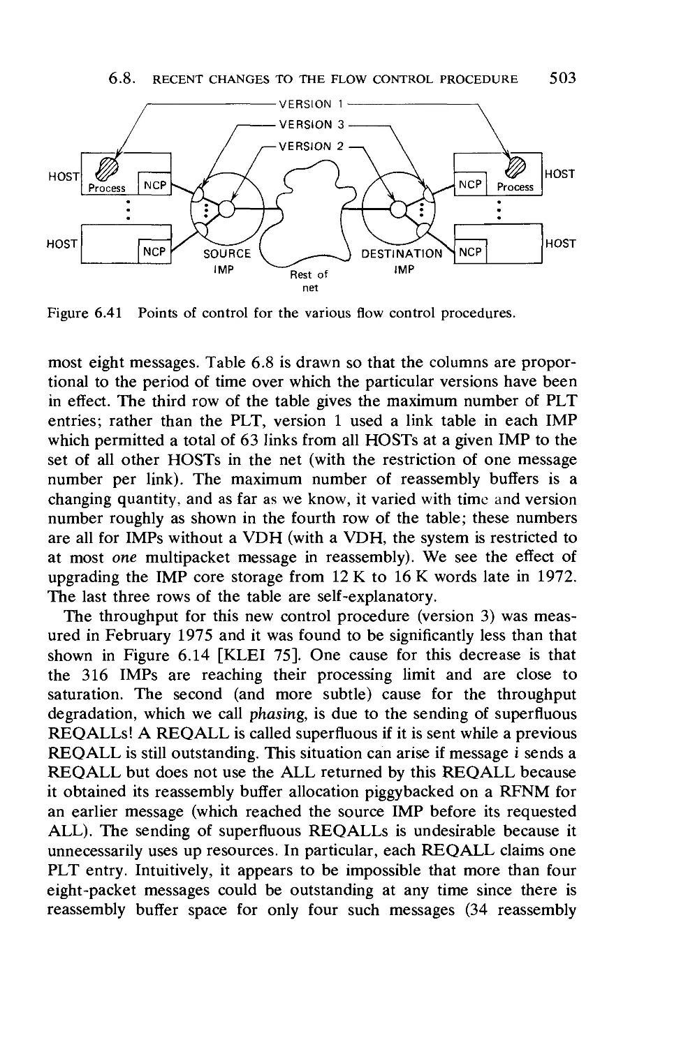
/


Текст
QUEUEING SYSTEMS
Volume 2: COMPUTER APPLICATIONS
8&s£:'f:?-
■* -T ■'"■ <
im
^%fti>f%
-»Xs-
.-*&&,..
$■ ^ -A- ^.\r>r#% ^Jv* ^f Tat-1 t^tfci. ' L *fc *■
v ■ .-• ■■■'.-■ :v'j- -%-< .-> —
iff-;?
,\
*,-;
>^, /■:
'?■
s.
J
/a
Leonard Kleimock
QUEUEING SYSTEMS
VOLUME II: COMPUTER APPLICATIONS
"As gold which he cannot spend will make no man rich,
so knowledge which he cannot apply will make no man wise."
Samuel Johnson: The Idler No. 84
QUEUEING SYSTEMS
VOLUME II:
COMPUTER APPLICATIONS
Leonard Kleinrock
Professor
Computer Science Department
School of Engineering and Applied Science
University of California, Los Angeles
A Wiley-Interscience Publication
JOHN WILEY AND SONS
New York • Chichester • Brisbane • Toronto • Singapore
Copyright © 1976 by John Wiley & Sons, Inc.
All rights reserved. Published simultaneously in Canada.
Reproduction or translation of any part of this work beyond
that permitted by Sections 107 or 108 of the 1976 United States
Copyright Act without the permission of the copyright owner
is unlawful. Requests for permission or further information
should be addressed to the Permissions Department, John
Wiley & Sons, Inc.
Library of Congress Cataloging in Publication Data (Revised)
Kleinrock, Leonard.
Queueing systems.
"A Wiley-Interscience publication."
CONTENTS: v. 1. Theory.—v. 2. Computer applications.
1. Queueing theory. I. Title.
T57.9.K6 519.8'2 74-9846
ISBN 0-471-49111-X (v. 2)
Printed in the United States of America
20 19 18 17 16 15
TO STELLA
Preface
Recently, I made the mistake of flying across the country in a Boeing
747. As a queueing systems analyst, I should have known better! As soon
as I arrived at the airport, I immediately realized my error, for there was
a mob of passengers waiting to be checked in. This was clearly a
rush-hour situation for the airline, and the peak load was saturating the
service facility. I, of course, had two extremely heavy suitcases filled with
notes on queueing systems (what else?) and so I could not morally avoid
this queue. The situation was a multiple-server multiple-queue system with
clearly unequal rates of service; however, once invested in a (particularly
slow) queue, I could not afford to risk giving up my position. After
clearing the check-in procedure, I then found my way to the departure
lounge where an enormous queue had been formed in a snakelike
fashion awaiting seat assignments and boarding passes. This was a two-
server system with a common queue that also was unbelievably
overloaded. The snaked queue convoluted itself in such a way that its tail was
immediately adjacent to its head, so, as you might imagine, considerable
cheating took place as passengers bypassed the queue completely; there
was absolutely no control of this effect except for a few angry passengers
(however, those at the head of the queue who were in the only position to
stop this cheating really did not care since they were ready to be served at
this point). Aboard the aircraft, of course, things went from bad to worse
as the overworked crew provided a comedy of errors and a tragedy of
frustrations for all of us. Would you believe that one of the meals was
served in buffet fashion so that the entire passenger population was asked
to stand up and file past a collection of randomly placed delicacies in the
lounge at the front of the aircraft? The ingenuity of this last queue was
too much for me. They arranged matters so that first those passengers on
the port side of the aircraft queued up in the port aisle, worked their way
to the front, received (fought for) the delicacies, returned via the
starboard aisle, and then found it quite impossible to reach their seats
because of the port aisle queue. A similar delight later developed for the
passengers on the starboard side. I was foolish enough to suggest the
vn
Vlll PREFACE
obvious improvement whereby port-side passengers would queue up on
the starboard aisle, leaving their own aisle clear for return to their seats,
but was quickly informed that such a suggestion "could not possibly
work!" And so it continued up to and including baggage recovery (you
can imagine the fun).
That travel adventure is just one of many similar situations that all of
us have encountered. As systems analysts, we have a moral and personal
obligation to study these real-life systems and provide some relief from
their aggravations even if they do not lend themselves easily to analysis.
We should be able to develop models for the physical systems we interact
with, produce an analysis that describes the behavior of these systems,
and then find methods for improving their behavior. In so doing, the first
task of creating the mathematical model is perhaps the most difficult,
since it is here that we make the most compromises in describing the
reality of the physical systems. In the second (analytical) stage, we look
for tools to aid us in solving these systems, and in the third we look for
design methodologies. For many of the technological systems of today, we
find that tools from queueing theory are useful in describing the systems'
behavior. Unfortunately, these tools are not nearly as sharp as we would
like, and so we often are faced with the necessity of using tools that are
not wholly adequate for the job. This is a common problem whenever one
deals in applications of a theory, and it is our purpose in this book to
study the difficulty and the success in the application of queueing systems
to various fields, and in particular to the field of computer systems.
The class of systems that generally lends itself to queueing analysis is
the (huge) one in which customers compete for access to a limited (i.e.,
finite-capacity) resource. In fact, many of today's significant problems can
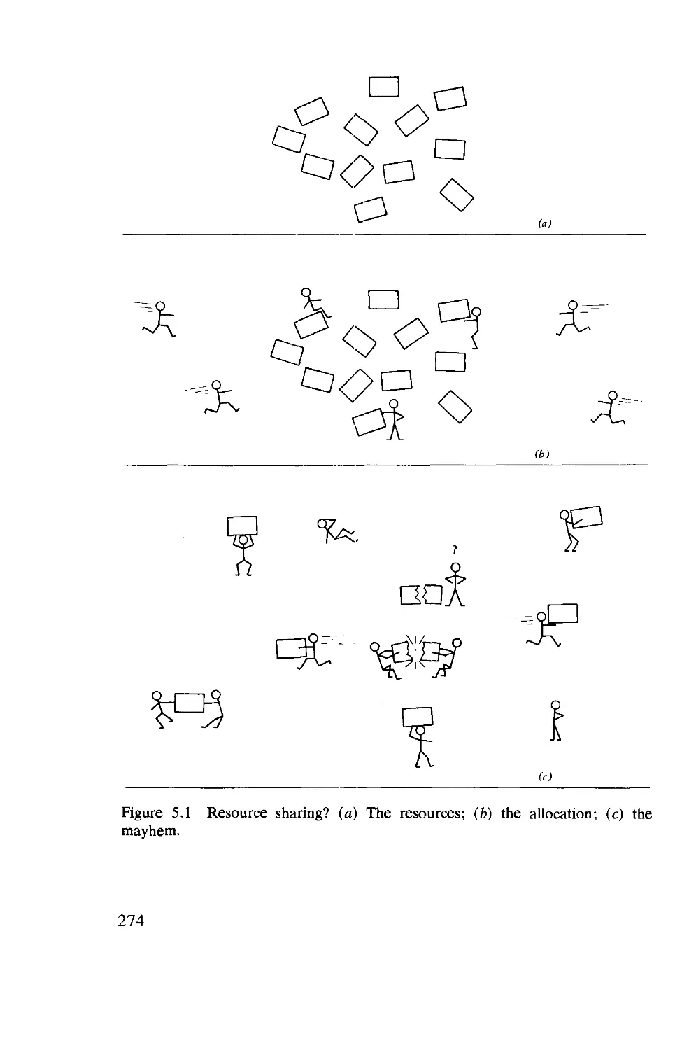
be reduced to the problem of resource allocation and resource sharing.
Throughout this book, we will encounter such problems, and we will
emphasize the need for resource; sharing in computer systems for
purposes of efficiency. For example, imagine that a pair of users requires the
use of a communication channel. The classical approach to satisfying this
requirement is to provide a channel for their use as long as that need
continues (and to charge them for the full cost of this channel). It has long
been recognized that such allocation of scarce resources is extremely
wasteful, as witnessed by their low utilization. Rather than provide
channels on a user-pair basis, we much prefer to provide a large
number of users with a single high-speed channel that can be shared in some
fashion; this then allows us to take advantage of the powerful "large-
number laws" which state that, with very high probability, the demand at
any instant will be very nearly equal to the sum of the average demands
of that user population. In this way, the required channel capacity to
PREFACE IX
support the user traffic may be considerably less than in the unshared case
of dedicated channels. This approach has been used to great effect for
many years now in a number of different contexts; for example, in the
use of graded channels in the telephone industry, in the introduction of
asynchronous time-division multiplexing, in the implementation of time-
shared and multiaccess computer systems, and in the packet-switching
concepts introduced in the 1960s and recently implemented in the
ARPANET. The essential observation is that the full-time allocation of a
fraction of the channel to each user-pair is highly inefficient compared to
the part-time use of the full capacity of the channel (this is precisely the
notion of time-sharing). We gain this efficient sharing particularly when
the traffic consists of rapid but short bursts of data. The classical schemes
of synchronous time-division multiplexing and frequency-division
multiplexing are examples of the inefficient partitioning of channels for bursty
data sources. As soon as we introduce the notion of a shared channel in a
packet-switching mode, then we must be prepared to resolve conflicts that
arise when more than one demand is simultaneously placed upon the
channel. There are two obvious solutions to this problem: the first is to
"throw out" or "lose" any demands made while the channel is in use; and
the second is to form a queue of conflicting demands and serve them in
some order as the channel becomes free. The latter approach is that taken
in the ARPANET since storage may be provided economically at the
points of conflict. The former approach is taken in the ALOHA system,
which uses packet switching with radio channels; in this system, in fact, all
simultaneous demands made on the channel are lost. These concepts are
discussed in Chapters 5 and 6, and represent some of the more successful
modern applications of queueing theory.
Our purpose in this book, then, is twofold: first, to modify the tools of
queueing theory in a way that permits them to be applied to real-world
problems; and second, to make an extensive application of these tools to
various and important modern-day computer systems.* Indeed, one of
the fastest-growing industries and one of the most advanced technologies
of today is that of computer systems. Sad to say, the theory is badly
lagging behind the practice in this field, and we have not yet come up with
an acceptable measure of computer power. Thus we find a situation in
which one grasps for analytical tools in attempting to evaluate
performance of computer systems. Fortunately, in the early 1960s it was found
that queueing theory was an effective tool for studying the throughput,
response, and other measures of performance for computer systems.
* This twofold purpose is the reason why Chapter 2 (Bounds, Inequalities and
Approximations) was placed here in Volume II rather than in Volume I (Theory).
X PREFACE
Since that time, the queueing theory literature and the computer
applications literature have virtually exploded with analytic models for computer
systems, and in this book we focus on some of these recent and successful
applications. Indeed, for those readers who have invested considerable
time, effort, and even discomfort in developing a set of queueing-
theoretic tools, this text represents one payoff for that effort. Now, finally,
we have the opportunity to use these tools in real-life applications. We
have chosen computer applications in this book principally since these
applications are the most recent and most successful for the theory of
queues (and also because, in no small way, I personally have been deeply
involved in the application of the theory to these cases). In fact, the use of
queueing theory to analyze resource allocation and job flow through
computer systems is perhaps the only method available to computer
scientists in understanding the behavior of the complex interconnection of
their systems.
This book was written over a period of many years while being used as
class notes at the graduate level in the Computer Science Department of
the School of Engineering and Applied Science at the University of
California, Los Angeles. Much of this material has come to life in the
course of this development and in the participation of UCLA as a
modeling and analysis center for research in computer systems. A vast
number of important problems have been identified as a result of these
applications and many opportunities exist for the clever and capable
analyst.
This book is at the first-year graduate level and naturally follows
material such as that contained in my companion volume, Queueing
Systems, Volume I: Theory. In order that this stand on its own as a
self-contained book, we begin with a queueing theory primer in Chapter 1
in which we review the fundamental material in queueing systems
analysis. Those readers who have been exposed to a first course in
queueing systems will easily manage the material in this book. On the
other hand, for those readers who have not been through a formal course
in queueing systems, this book is well within their reach if they accept the
material presented in Chapter 1 as a point of departure for the balance of
the book.
Chapter 2 is the bridge that permits us to pass from the abstract tools
of queueing theory to the real world of applied results. In this chapter, we
acknowledge the weaknesses and shortcomings of the formal theory in its
ability to describe the real-world applications that we encounter;
consequently, we look for engineering guidelines in the form of bounds,
inequalities, and approximations that are permissible and valid in various
situations. Following that, we discuss the interesting field of priority
PREFACE XI
queueing in Chapter 3. We look upon this chapter as a further bridge
between theory and applications, since it is through priority queueing that
we are able to model the behavior of computer time-sharing and
multiaccess systems, which form the subject material for Chapter 4. In this, our
first real applications chapter, we emphasize computer systems in
isolation that handle demands from a large collection of competing users. We
look for throughput and response time as well as utilization of resources.
The major portion of this chapter is devoted to a particular class of
algorithms known as processor-sharing algorithms, since they are
singularly well suited to queueing analysis and they capture the essence of
more difficult and more complex algorithms seen in real scheduling
problems. Chapter 5 addresses itself to the analysis and design of
computer-communication networks. In Chapter 6 we discuss simulation,
measurement, flow control, and traps in computer-communication
networks. These networks represent perhaps the fastest-growing field in the
young computer industry itself. In the Epilogue of Volume I, we
promised only one chapter in Volume II on computer networks; however, in
the months that separated the preparation of these two volumes, the field
has expanded so quickly that we have been forced to meet the challenge
of this material with an additional chapter. If the reader glances at the list
of references for these last two chapters, he will see that the majority are
drawn from the last three or four years—a tell-tale indicator indeed; as a
result, it is virtually impossible to produce a truly up-to-date chapter in a
printed volume such as this. Perhaps the best solution is to keep an
updated on-line file that is accessible through a computer network!
Chapter 5 is devoted to developing methods of analysis and design for
computer-communication networks; it identifies many unsolved,
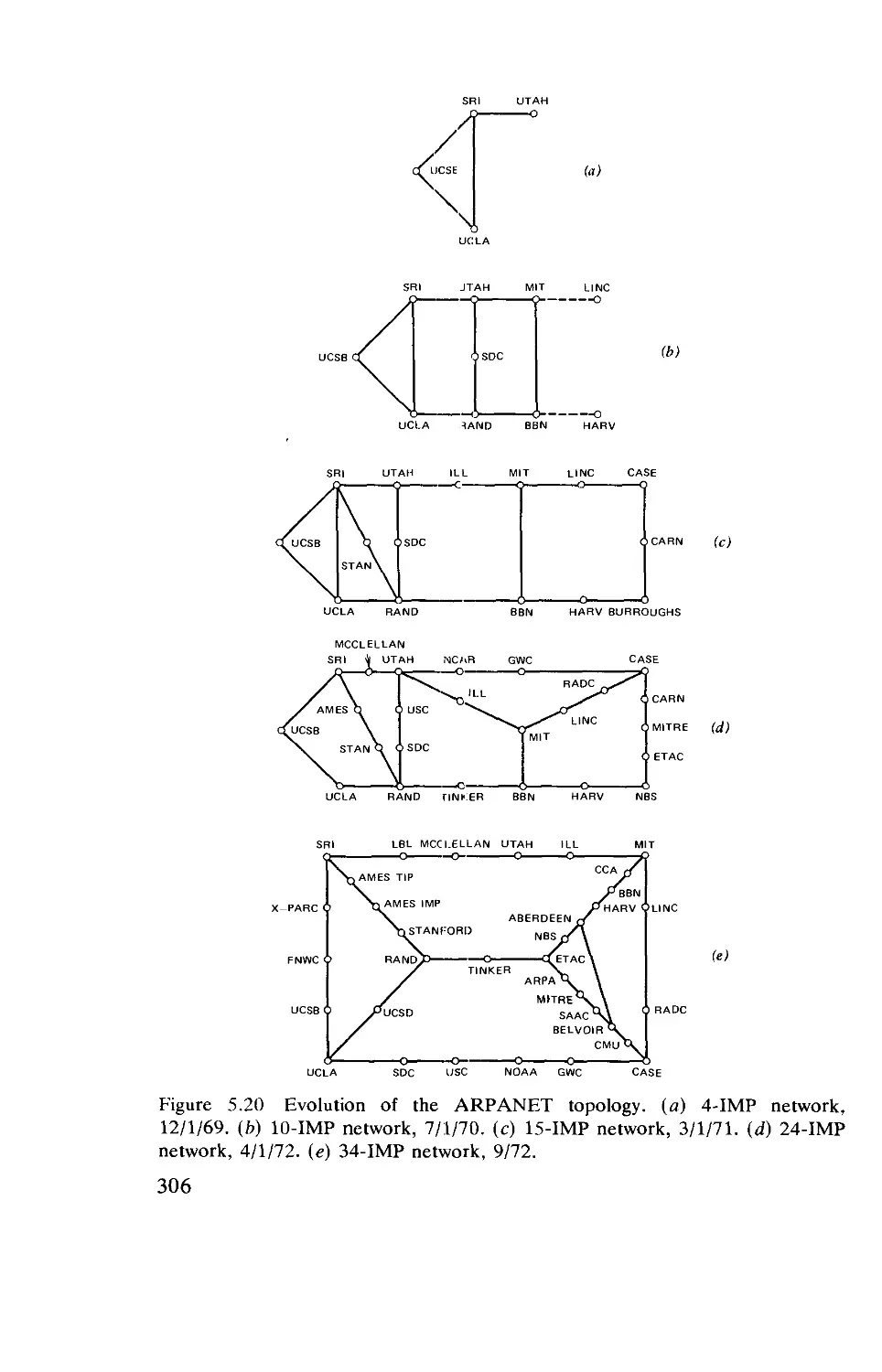
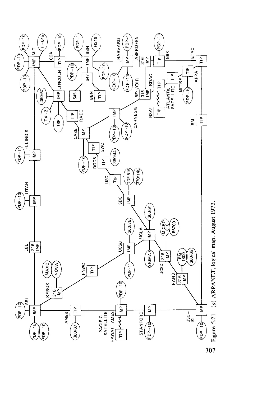
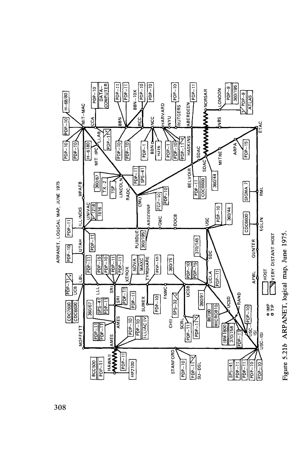
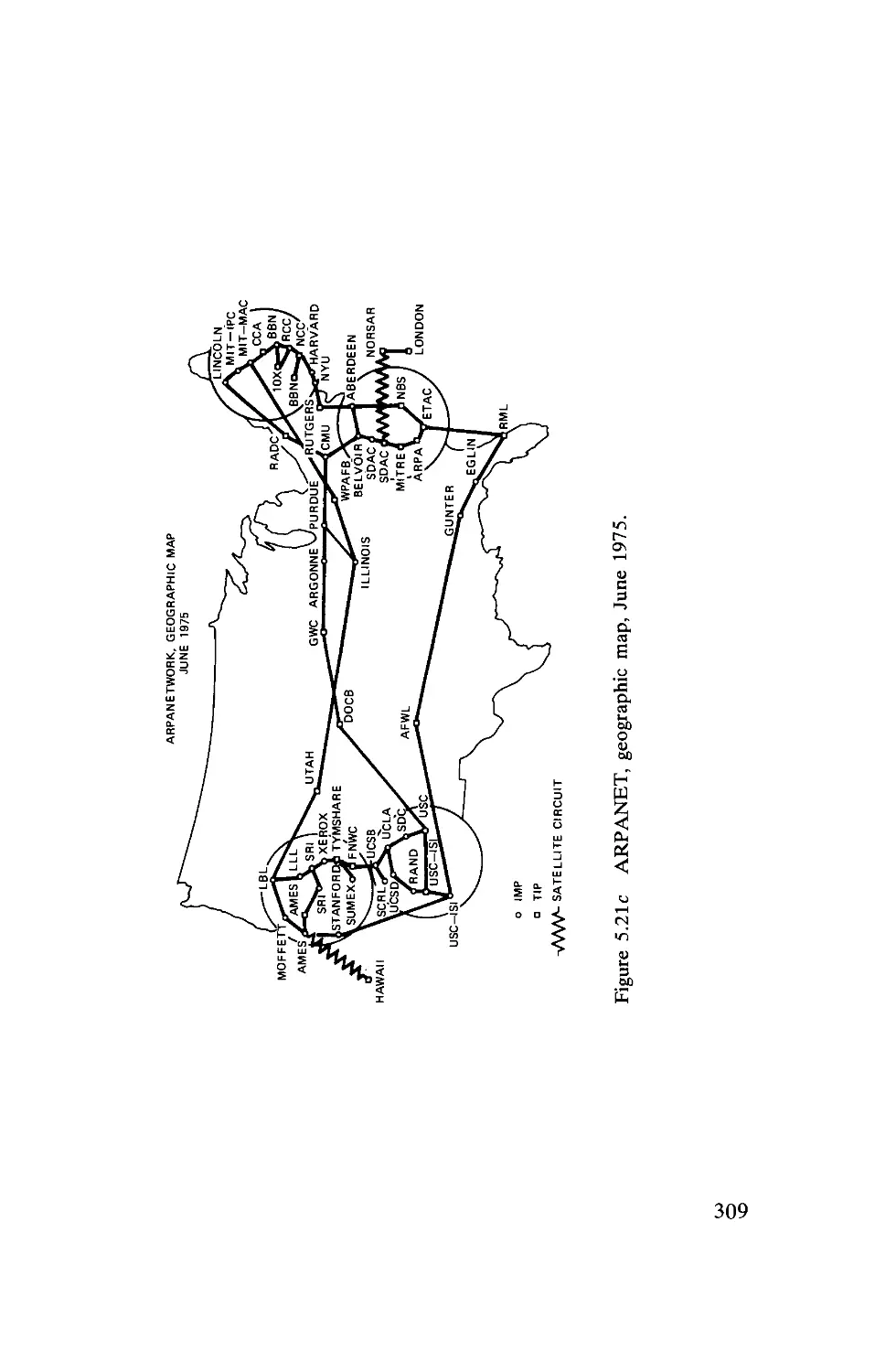
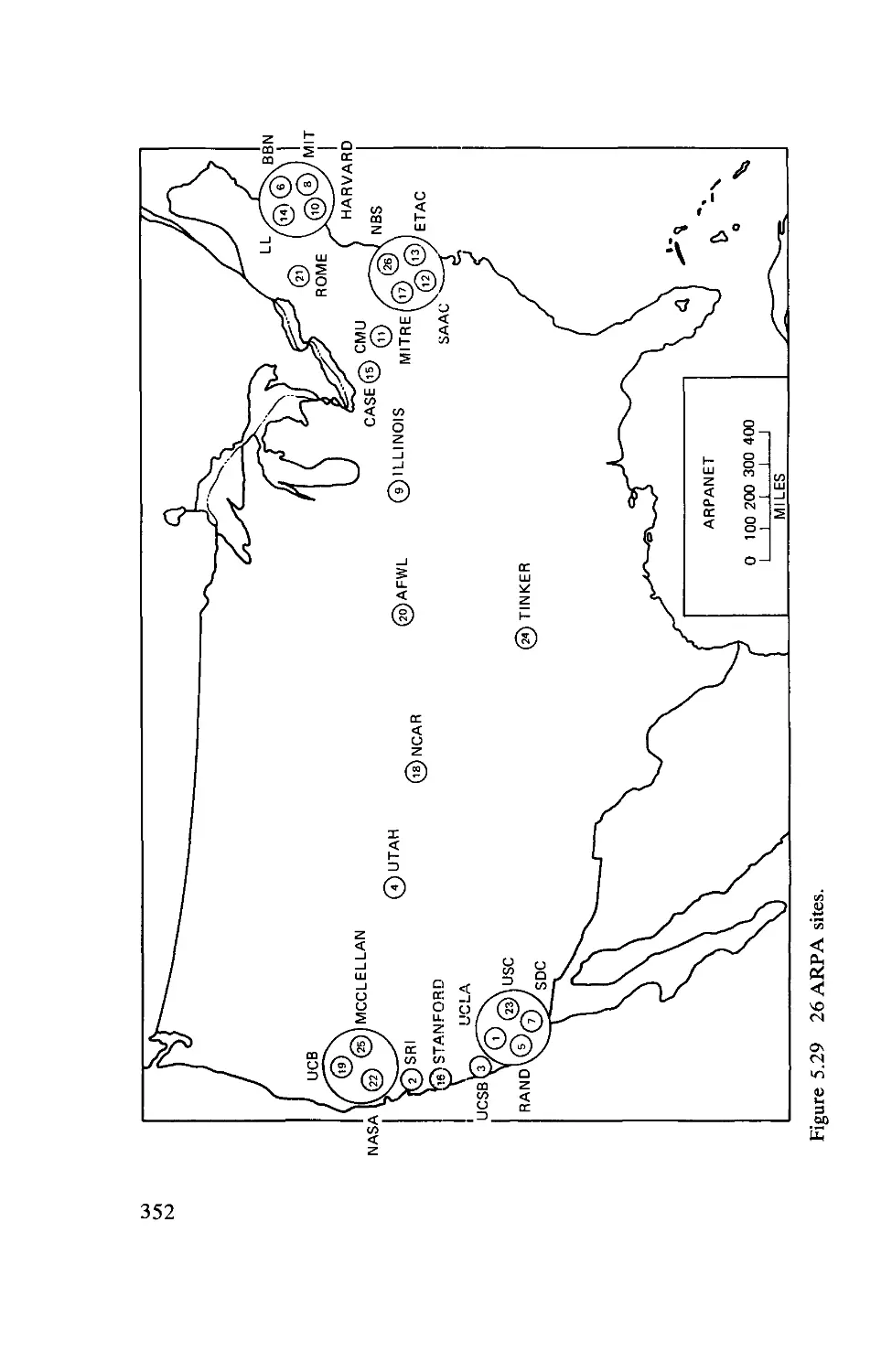
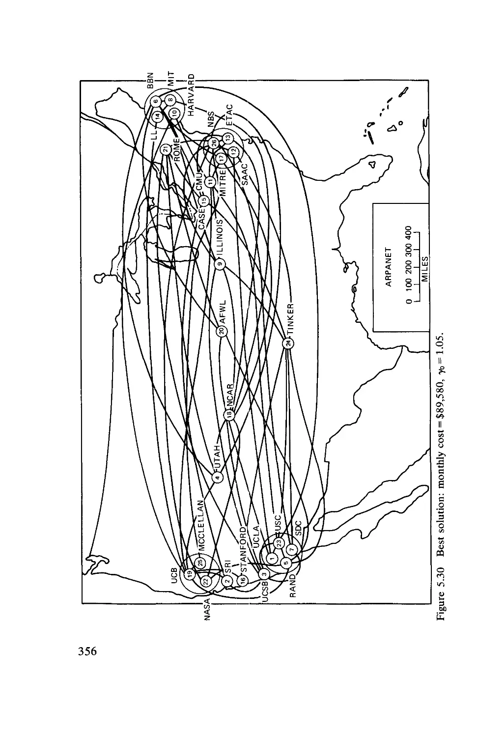
important problems. A specific existing network, the ARPANET, is used
throughout as an example to guide the reader through the motivation
and evaluation of the various techniques developed. The chapter closes
with the consideration of some of the newer packet-switching concepts,
namely, data transmission using satellite and ground radio
communications. Chapter 6 points to the operational and measurement aspects of
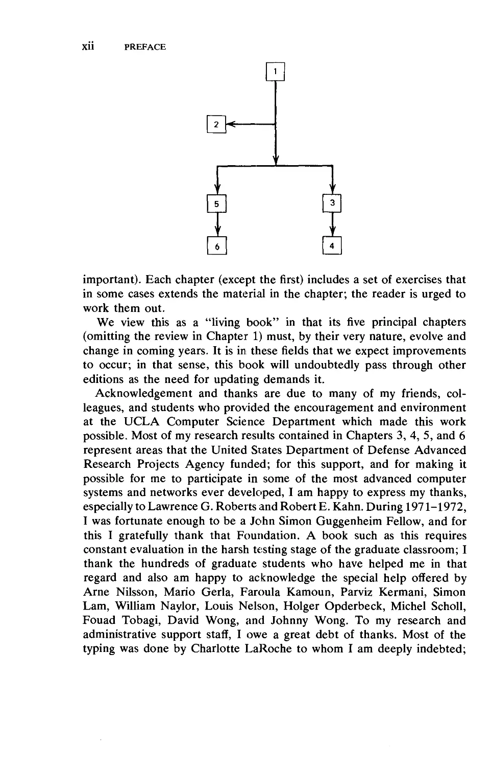
networks, drawing heavily from the ARPANET. On page xiv we show
the precedence structure among the chapters of this book.
A glossary at the end of the book summarizes the commonly used
symbols and notation. Each chapter contains its own list of references
keyed alphabetically to the author and year; for example, [KLEI 75]
would refer to the companion Volume I. All equations of importance
have been marked with a symbol ■, and these are included in the
summary of important equations (the equations in Chapter 1 are
exceptions to this in that the symbol is omitted, since all of them are
Xll PREFACE
1
2 ««■
f
i] 0
71 4
important). Each chapter (except the first) includes a set of exercises that
in some cases extends the material in the chapter; the reader is urged to
work them out.
We view this as a "living book" in that its five principal chapters
(omitting the review in Chapter 1) must, by their very nature, evolve and
change in coming years. It is in these fields that we expect improvements
to occur; in that sense, this book will undoubtedly pass through other
editions as the need for updating demands it.
Acknowledgement and thanks are due to many of my friends,
colleagues, and students who provided the encouragement and environment
at the UCLA Computer Science Department which made this work
possible. Most of my research results contained in Chapters 3, 4, 5, and 6
represent areas that the United States Department of Defense Advanced
Research Projects Agency funded; for this support, and for making it
possible for me to participate in some of the most advanced computer
systems and networks ever developed, I am happy to express my thanks,
especially to Lawrence G. Roberts and Robert E. Kahn. During 1971-1972,
I was fortunate enough to be a John Simon Guggenheim Fellow, and for
this I gratefully thank that Foundation. A book such as this requires
constant evaluation in the harsh testing stage of the graduate classroom; I
thank the hundreds of graduate students who have helped me in that
regard and also am happy to acknowledge the special help offered by
Arne Nilsson, Mario Gerla, Faroula Kamoun, Parviz Kermani, Simon
Lam, William Naylor, Louis Nelson, Holger Opderbeck, Michel Scholl,
Fouad Tobagi, David Wong, and Johnny Wong. To my research and
administrative support staff, I owe a great debt of thanks. Most of the
typing was done by Charlotte LaRoche to whom I am deeply indebted;
PREFACE Xlll
Carol Mason and Barbara Warren were responsible for handling my
unending revisions, and they were aided by Jean D'Fucci, Jean Dubinsky,
George Ann Hornor, Cathy Pfennig, and Gloria Roy. To Diana
Skocypec and Lynn Johnson fell the tedious task of proofreading the
garrulous galleys and ponderous pages; my admiration and thanks goes to
them. To my children, I offer my regret at having taken time for this
which might have been spent with them, and my thanks for their
indulgence. To my parents, I give my gratitude for the principles they
instilled in me and for the opportunities they afforded me. To Stella, my
wife, I owe much for her unending patience, encouragement, and
understanding, without which I could hardly have completed this work.
Leonard Kleinrock
Los Angeles, California
January 1976
CONTENTS
VOLUME II
Chapter 1 A Queueing Theory Primer
1.1. Notation
1.2." General Results
1.3. Markov, Birth-Death, and Poisson Processes
1.4. The M/M/l Queue
1.5. The M/M/m Queueing System .
1.6. Markovian Queueing Networks .
1.7. The M/G/l Queue
1.8. The G/M/l Queue
1.9. The G/M/m Queue
1.10. The G/G/l Queue
2
5
7
10
13
14
15
20
20
22
Chapter 2 Bounds, Inequalities and Approximations 27
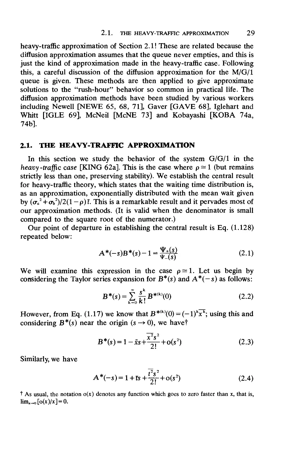
2.1. The Heavy-Traffic Approximation .... 29
2.2. An Upper Bound for the Average Wait ... 32
2.3. Lower Bounds for the Average Wait .... 34
2.4. Bounds on the Tail of the Waiting Time Distribution. 44
2.5. Some Remarks for G/G/m 46
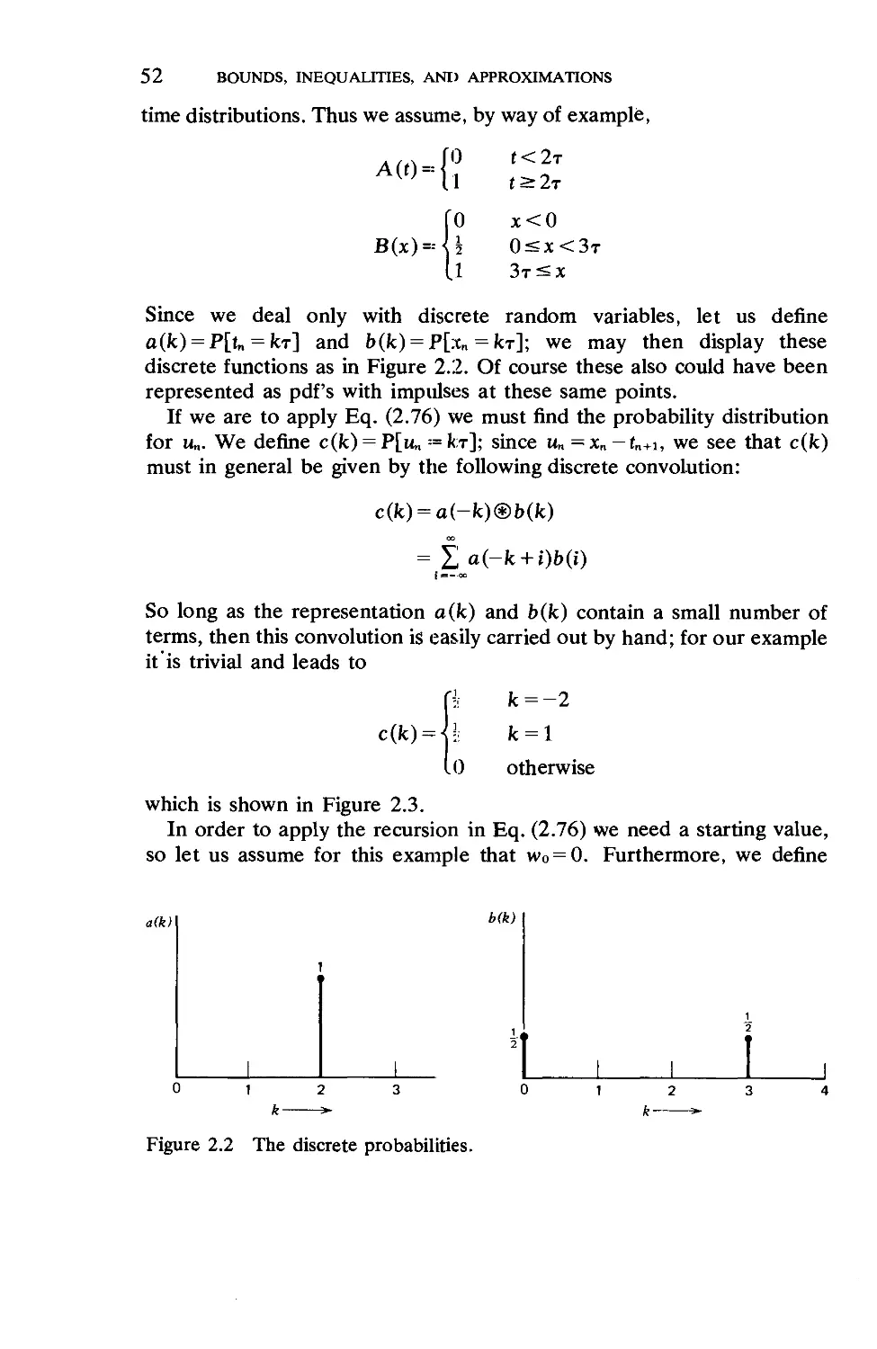
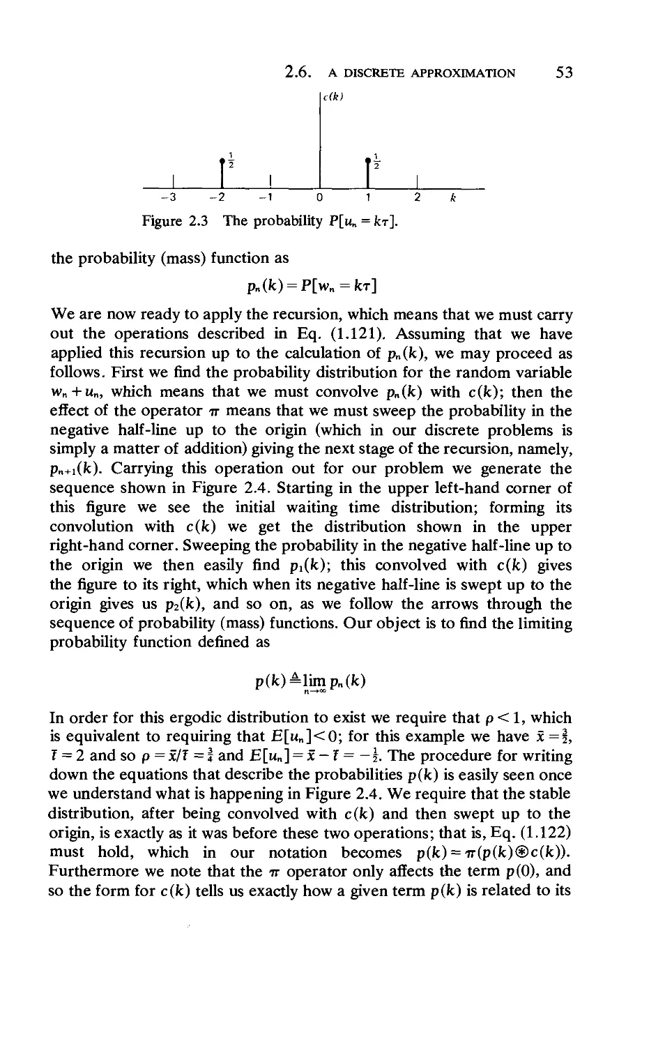
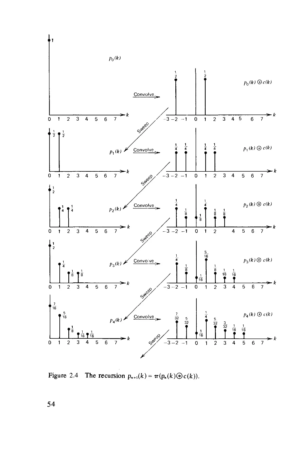
2.6. A Discrete Approximation 51
2.7. The Fluid Approximation for Queues. ... 56
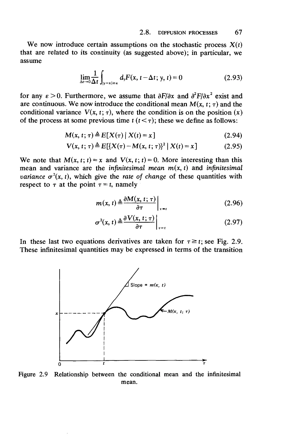
2.8. Diffusion Processes 62
2.9. Diffusion Approximation for M/G/l .... 79
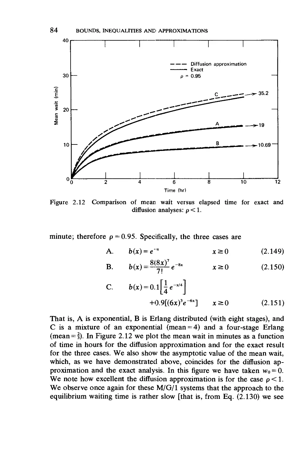
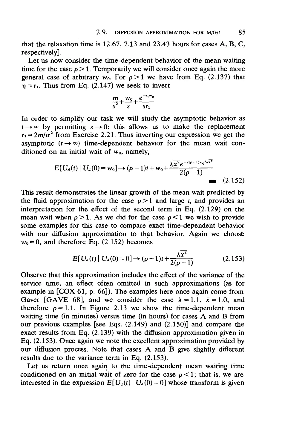
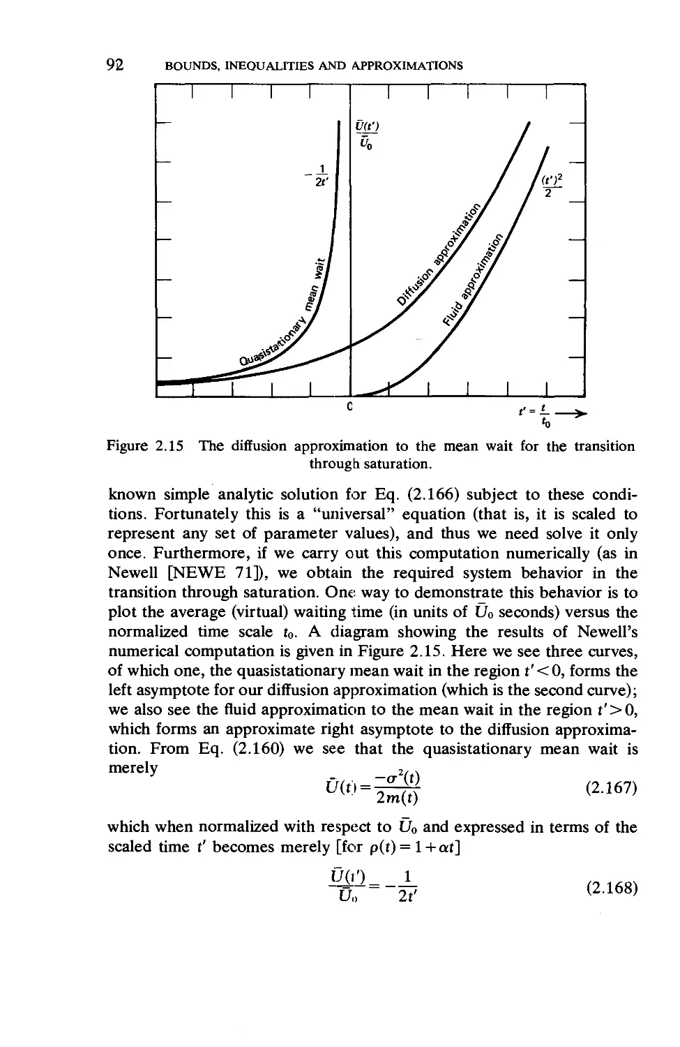
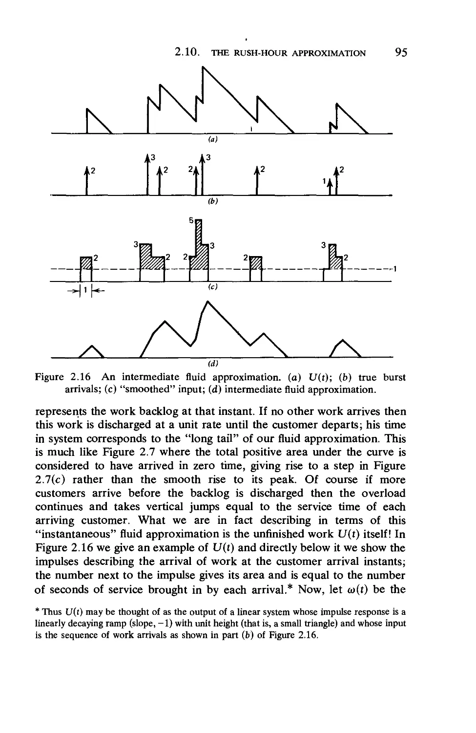
2.10. The Rush-Hour Approximation 87
Chapter 3 Priority Queueing
106
3.1. The Model 106
3.2. An Approach for Calculating Average Waiting Times 106
3.3. The Delay Cycle,Generalized Busy Periods, and
Waiting Time Distributions 110
xv
XVI CONTENTS
3.4. Conservation Laws
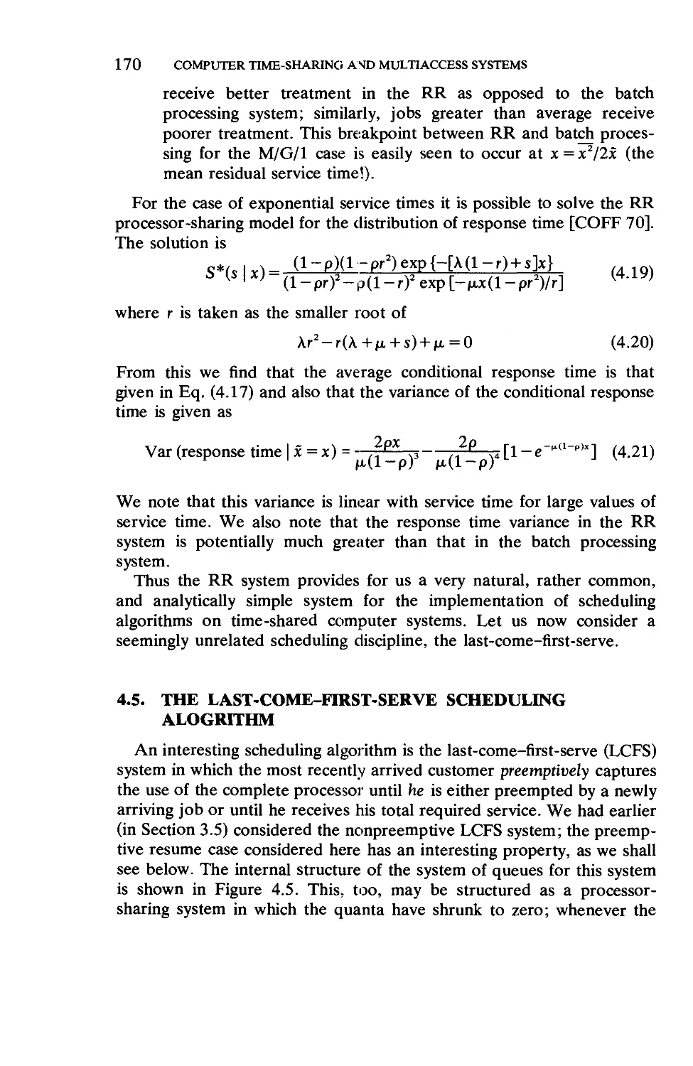
3.5. The Last-Come-First-Serve Queueing Discipline
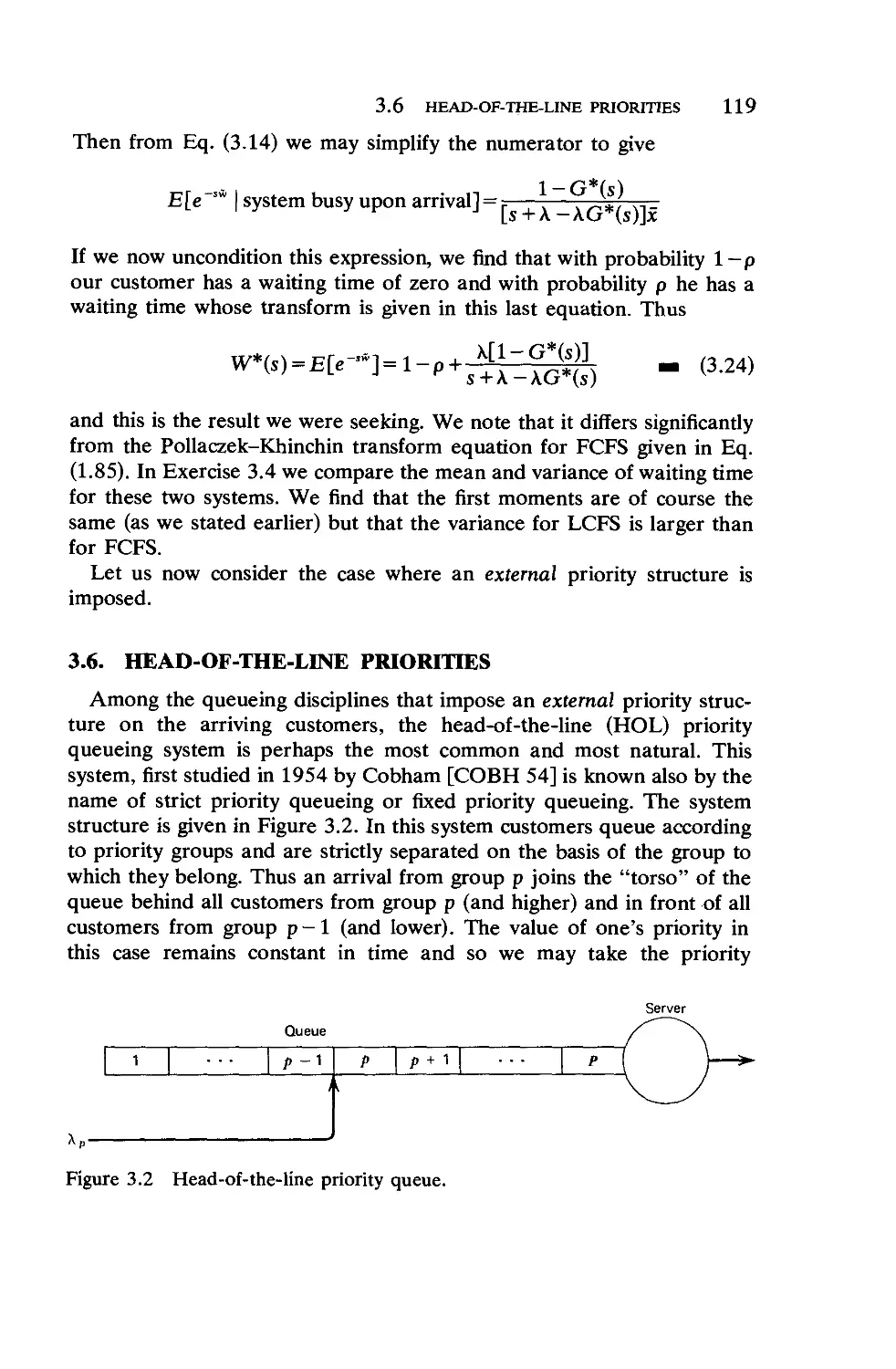
3.6. Head-of-the-Line Priorities
3.7. Time-Dependent Priorities
3.8. Optimal Bribing for Queue Position .
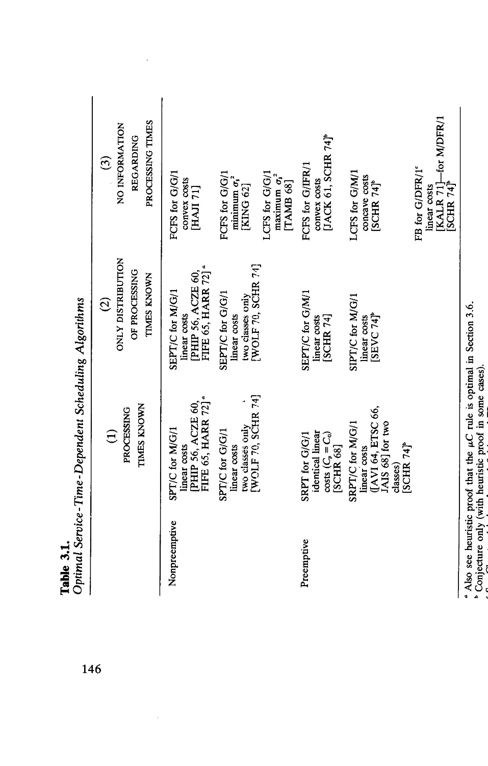
3.9. Service-Time-Dependent Disciplines .
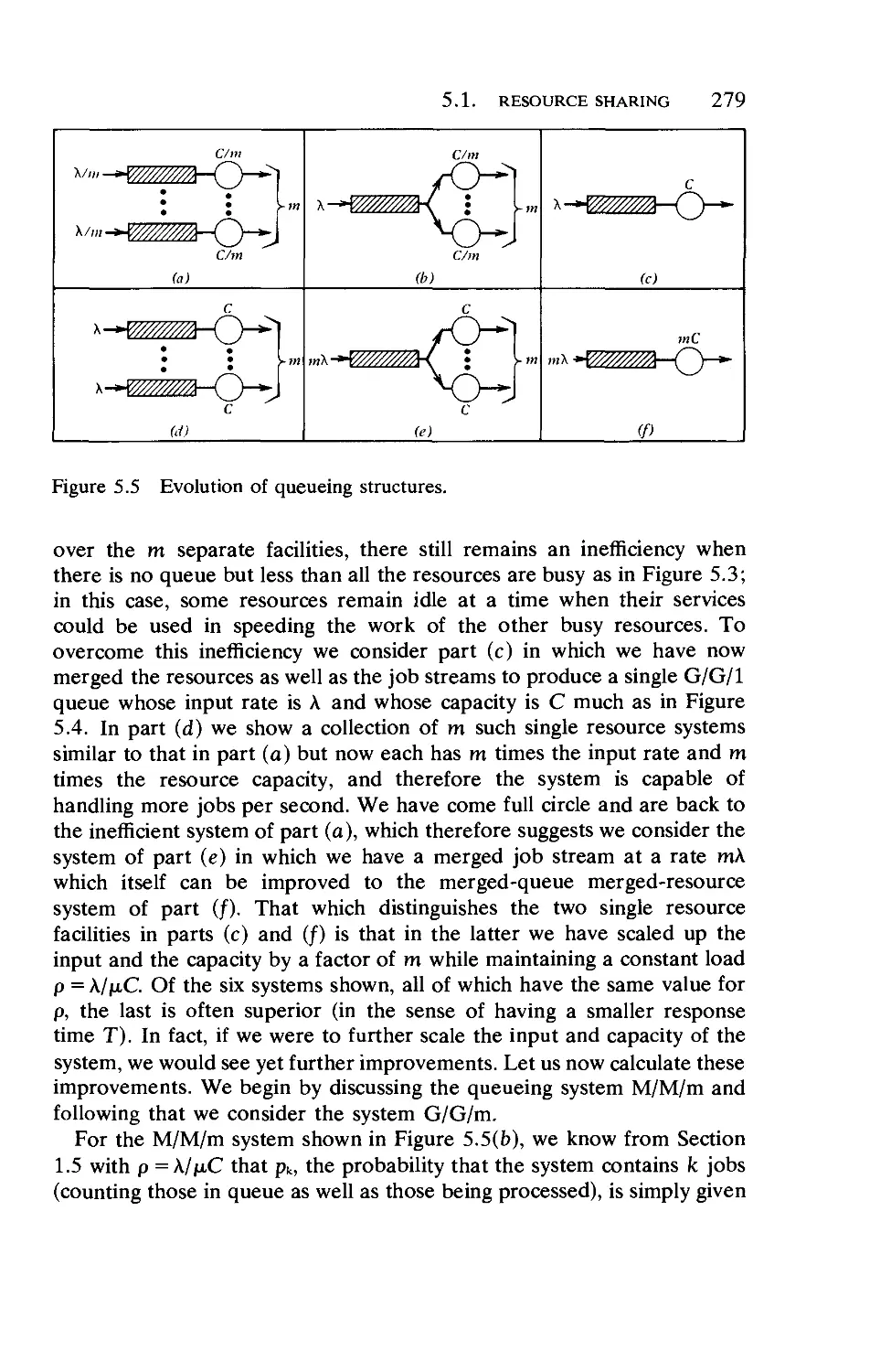
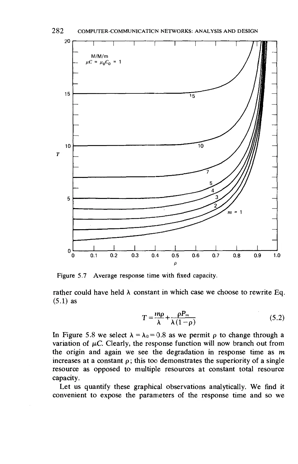
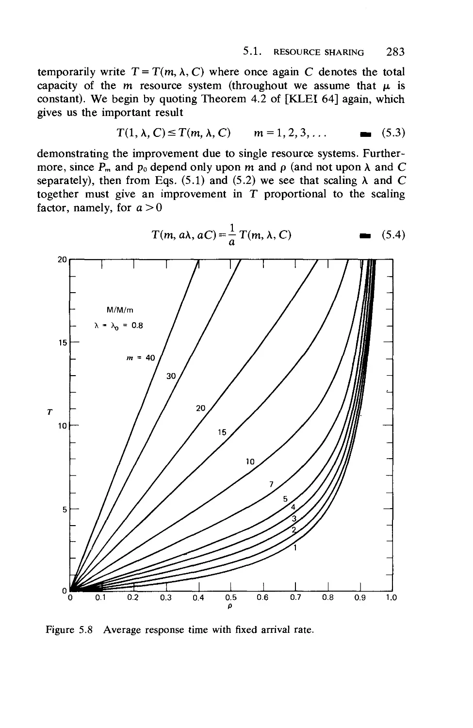
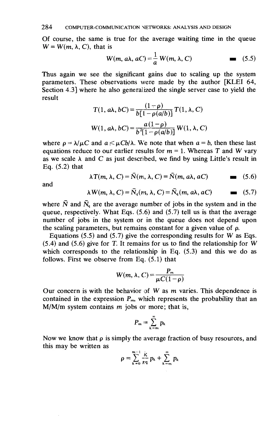
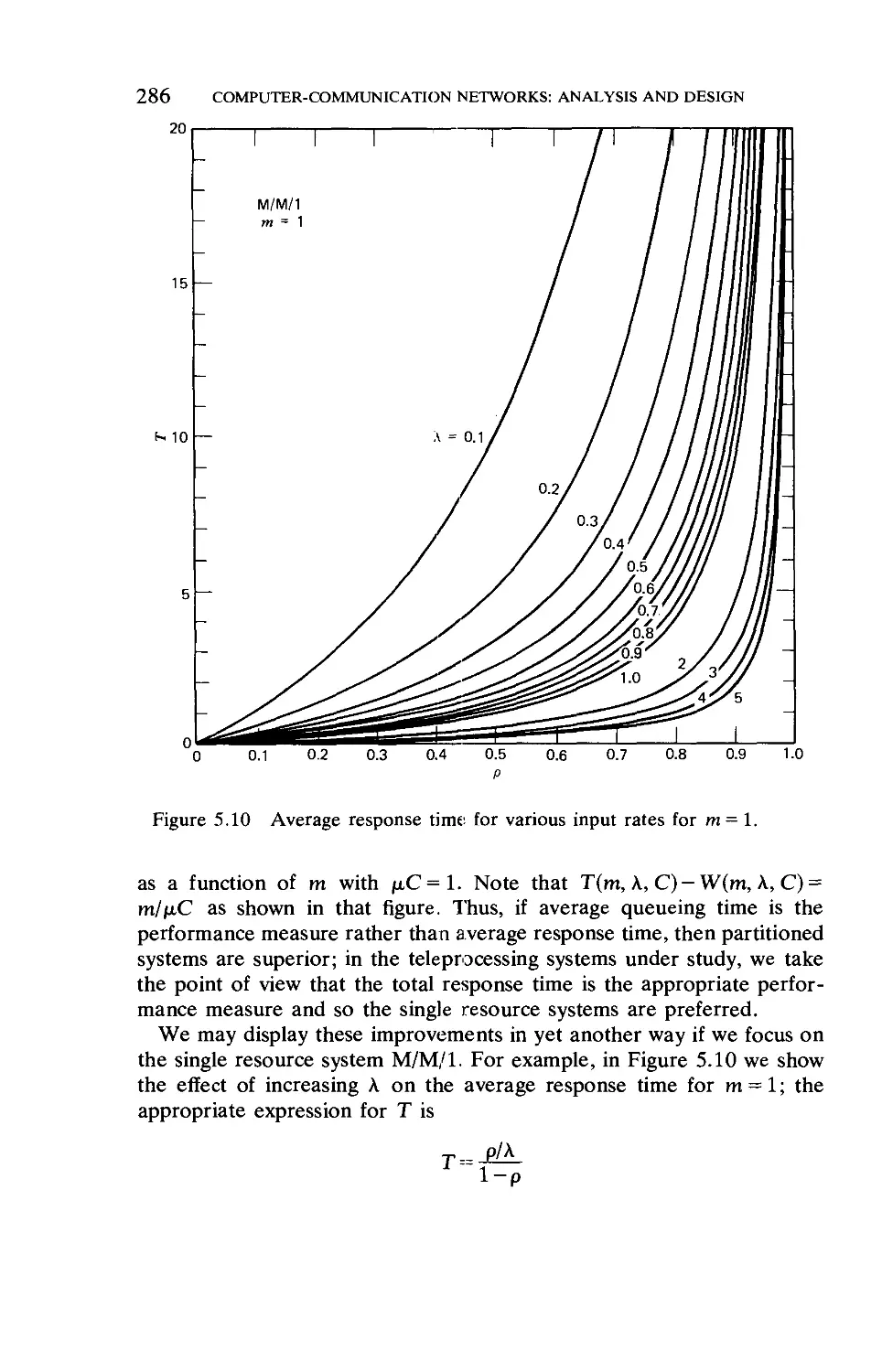
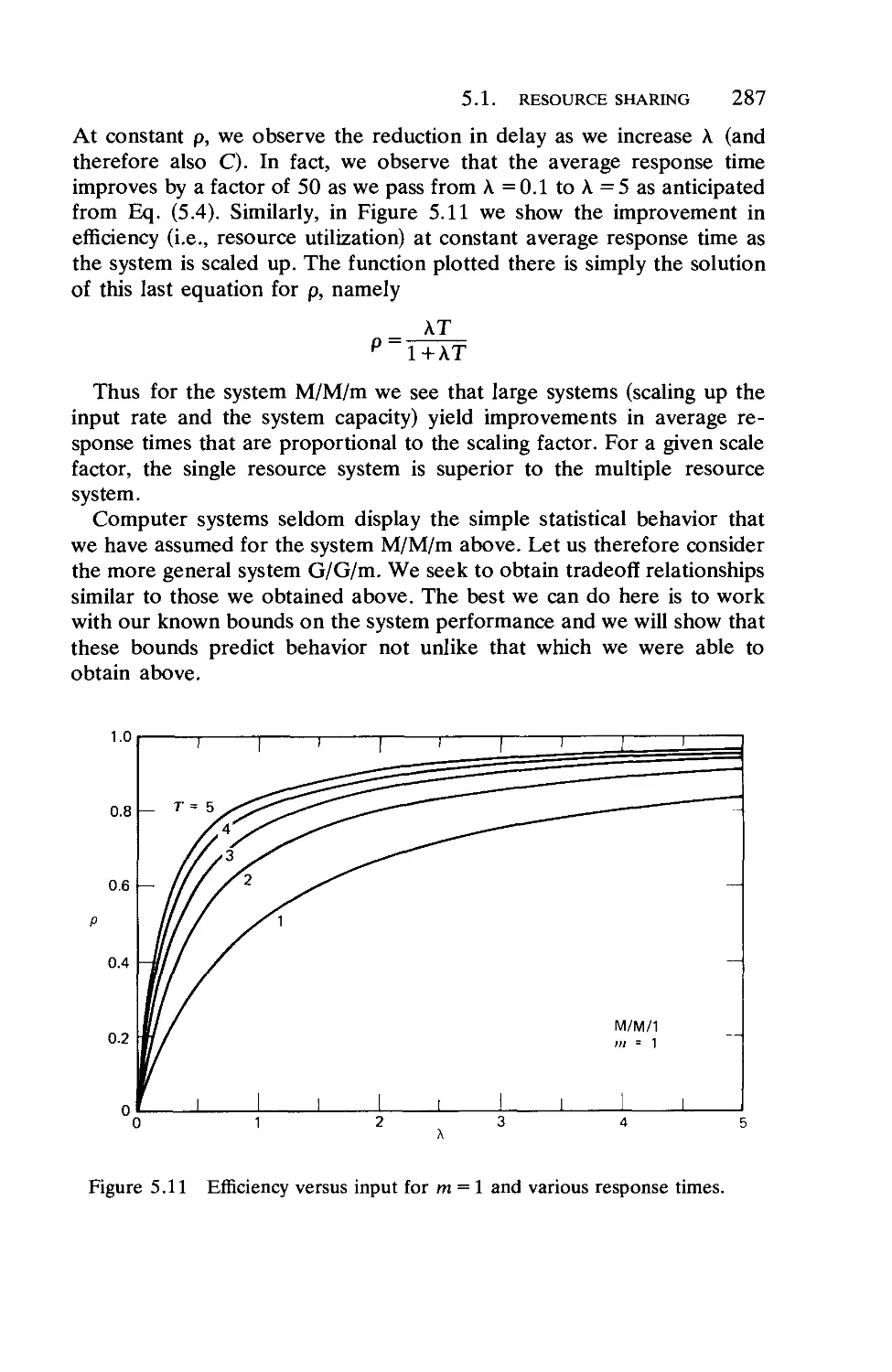
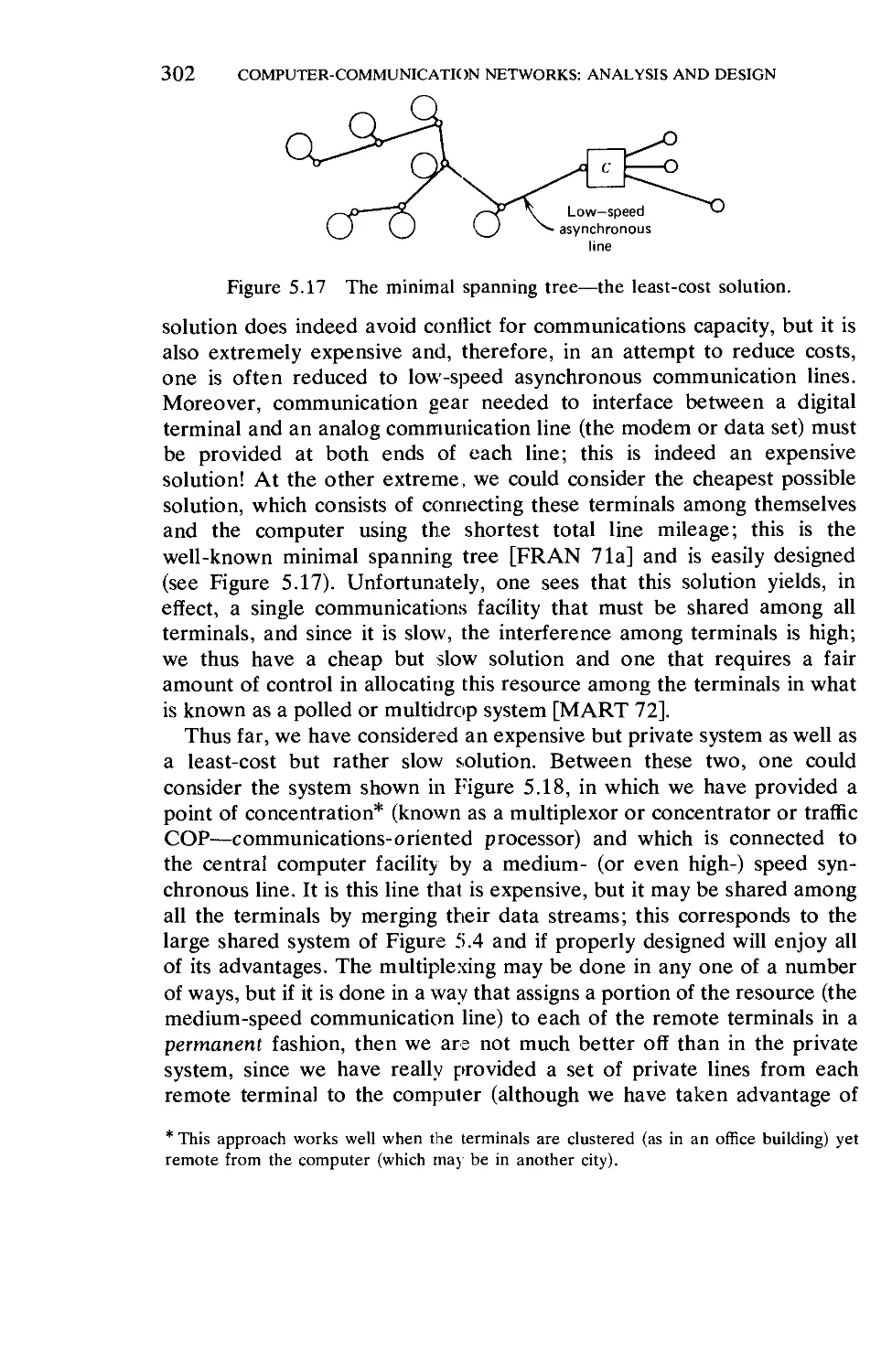
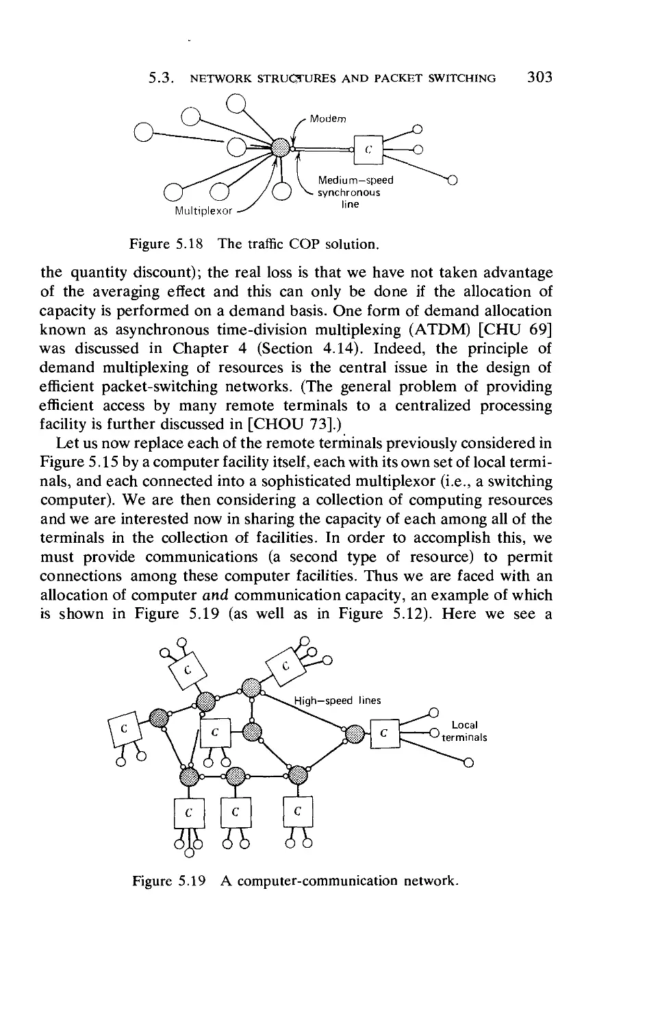
5.1. Resource Sharing
5.2. Some Contrasts and Trade-Offs .
5.3. Network Structures and Packet Switching .
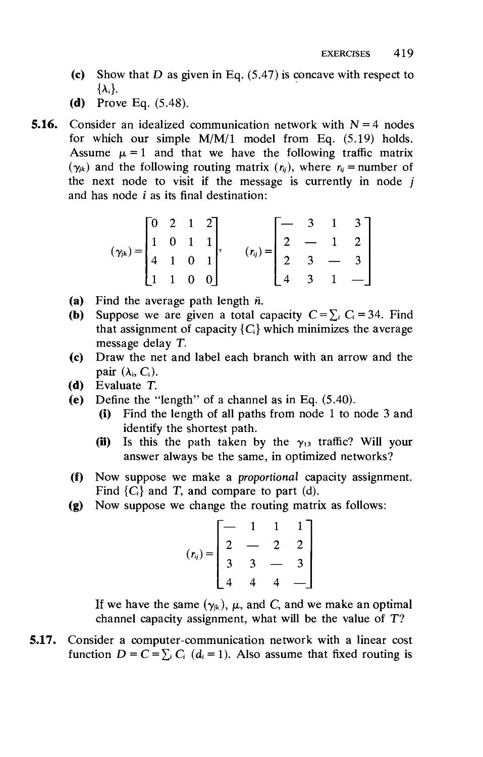
5.4. The ARPANET—An Operational Description
Existing Network
5.5. Definitions, Model, and Problem Statements
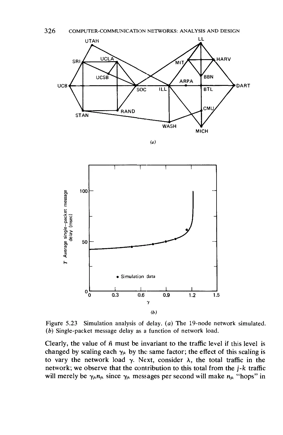
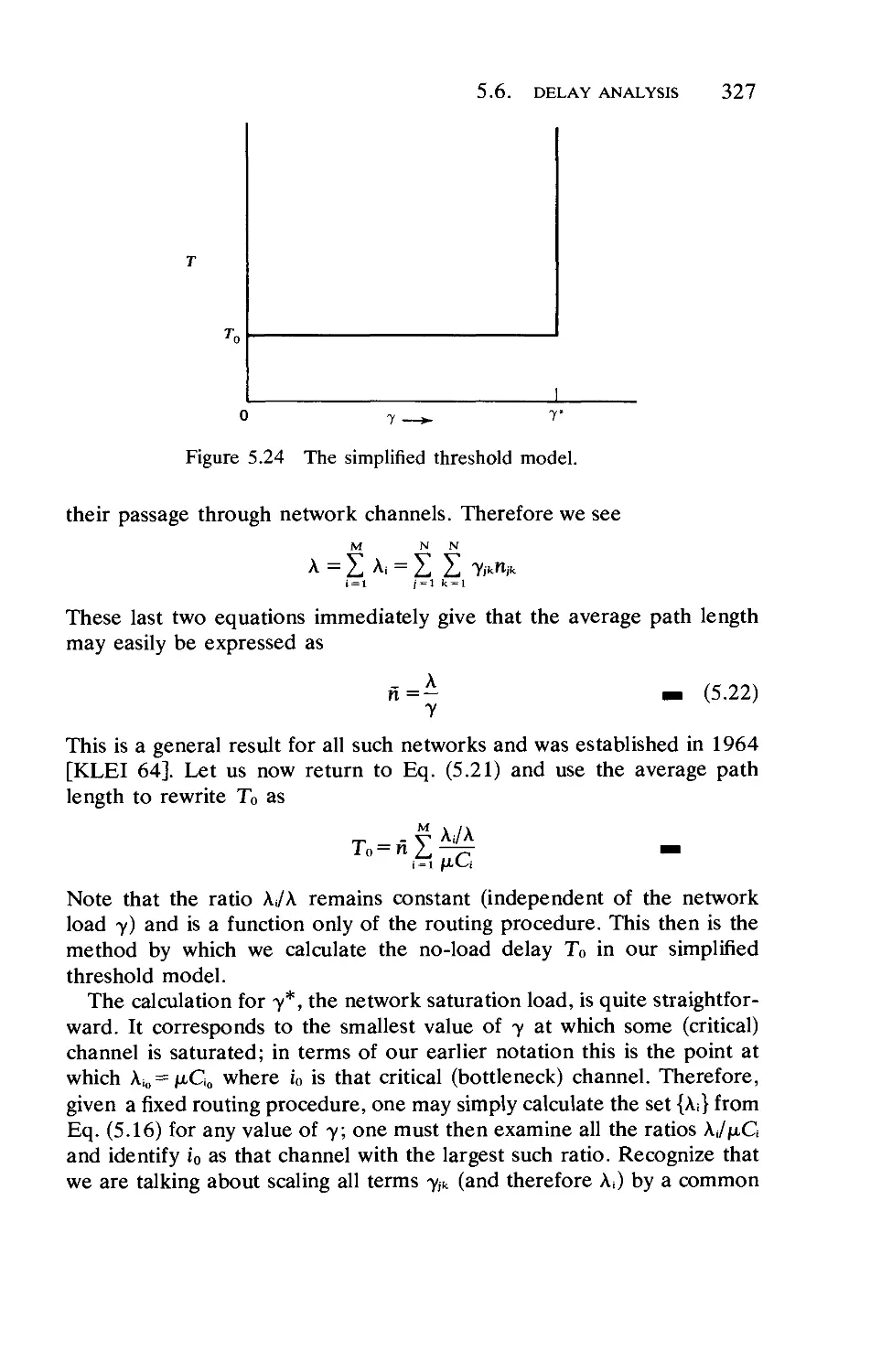
5.6. Delay Analysis
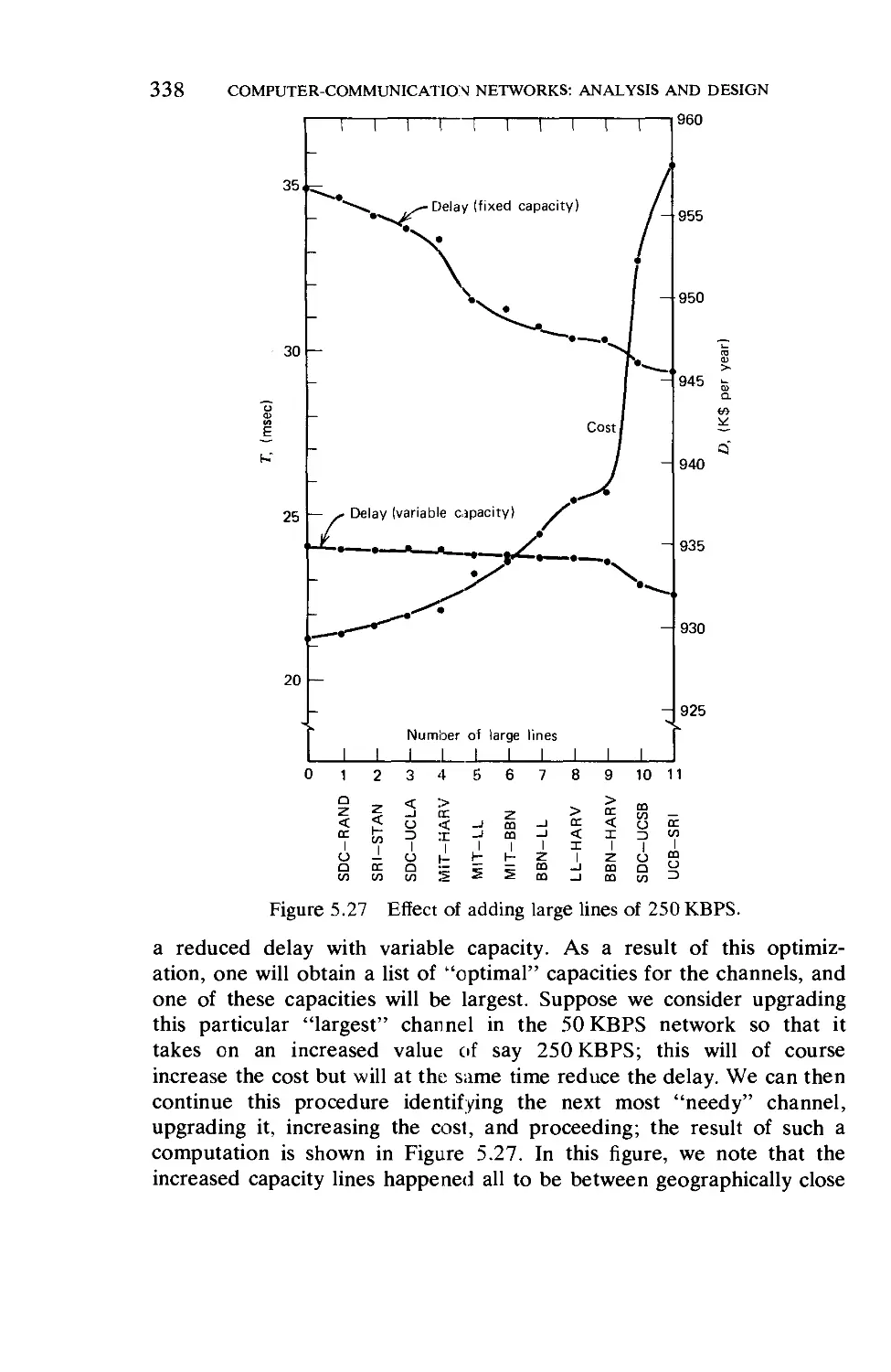
5.7. The Capacity Assignment Problem .
5.8. The Traffic Flow Assignment Problem
5.9. The Capacity and Flow Assignment Problem
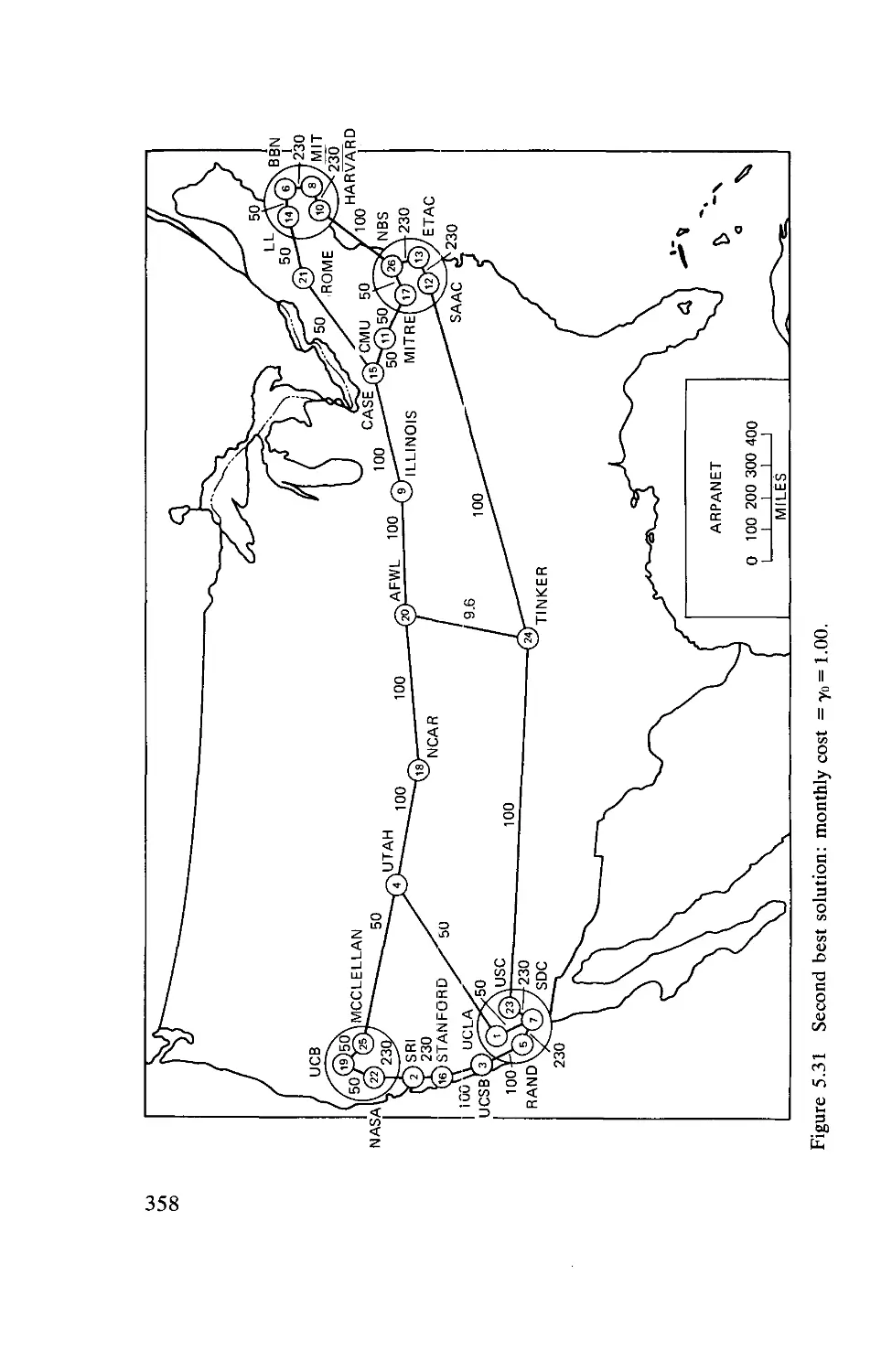
5.10. Some Topological Considerations—Applications
ARPANET
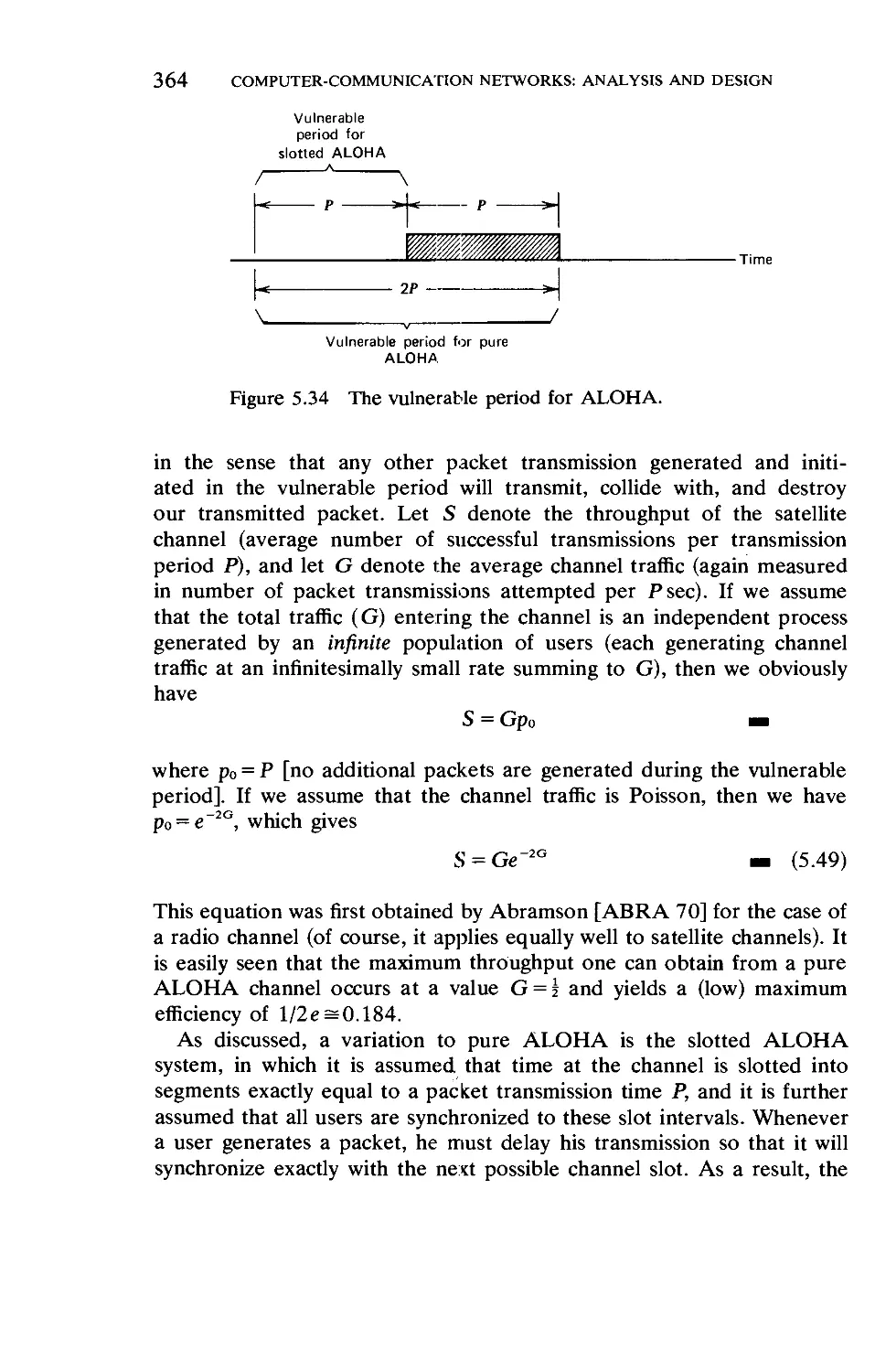
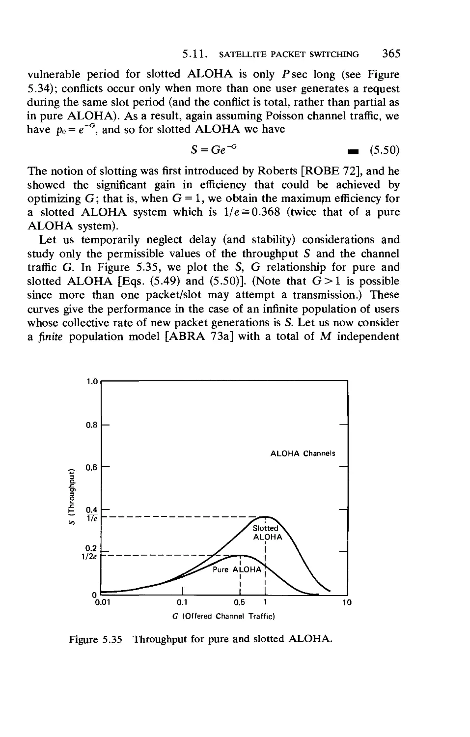
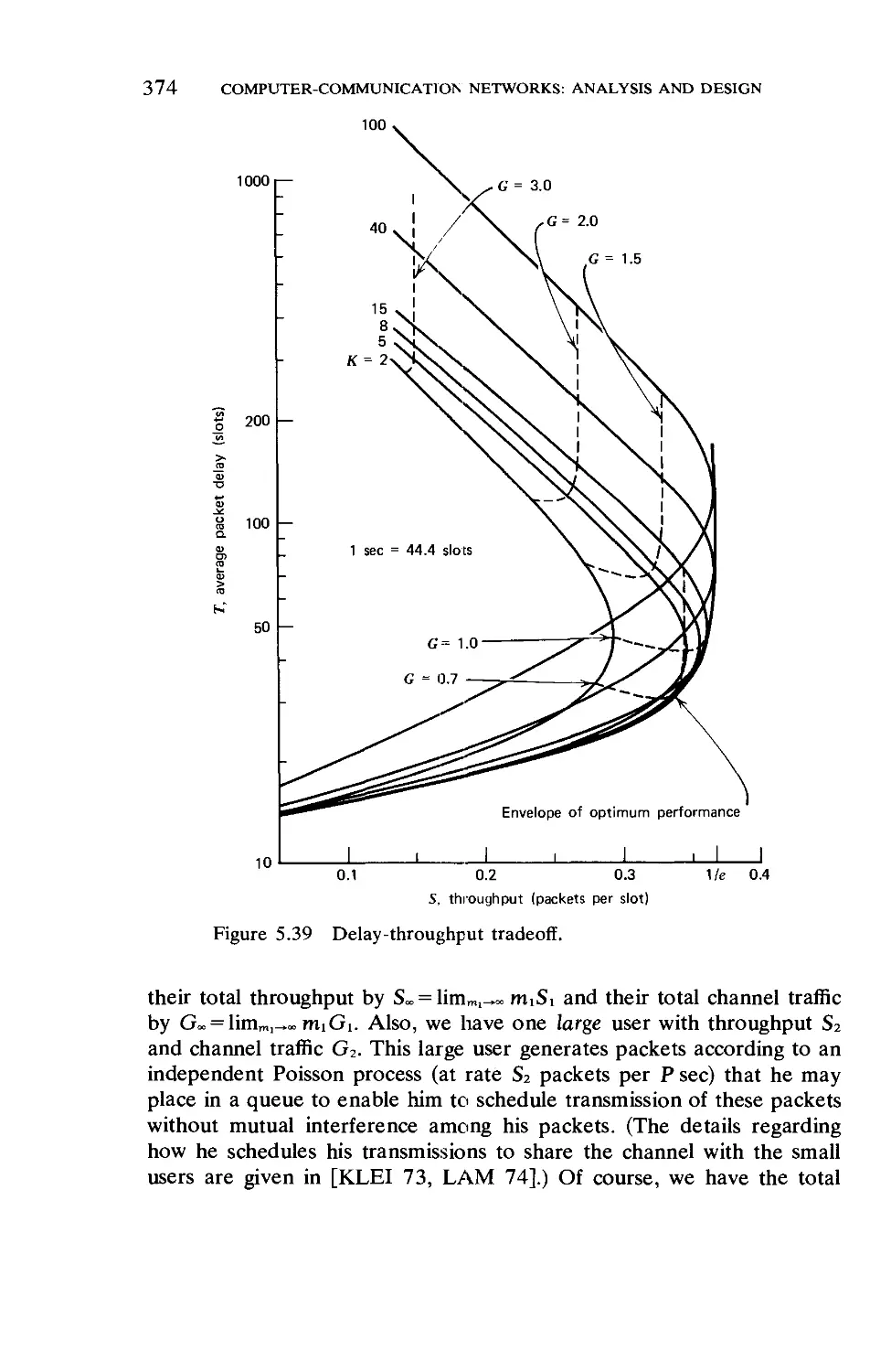
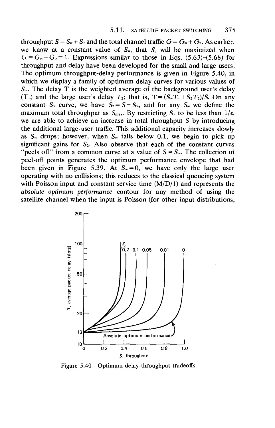
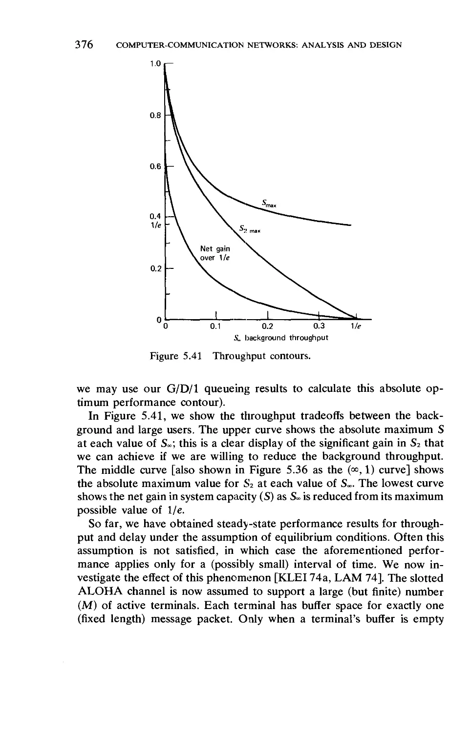
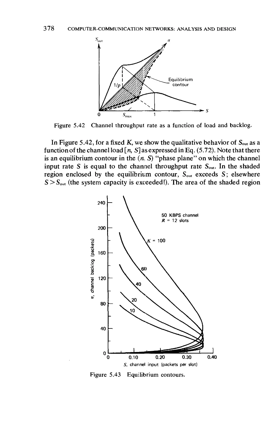
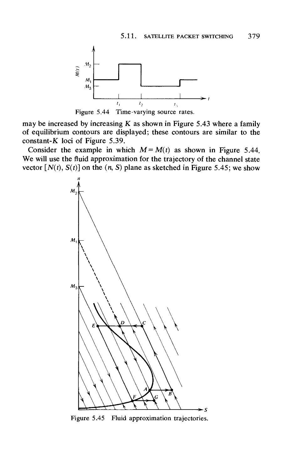
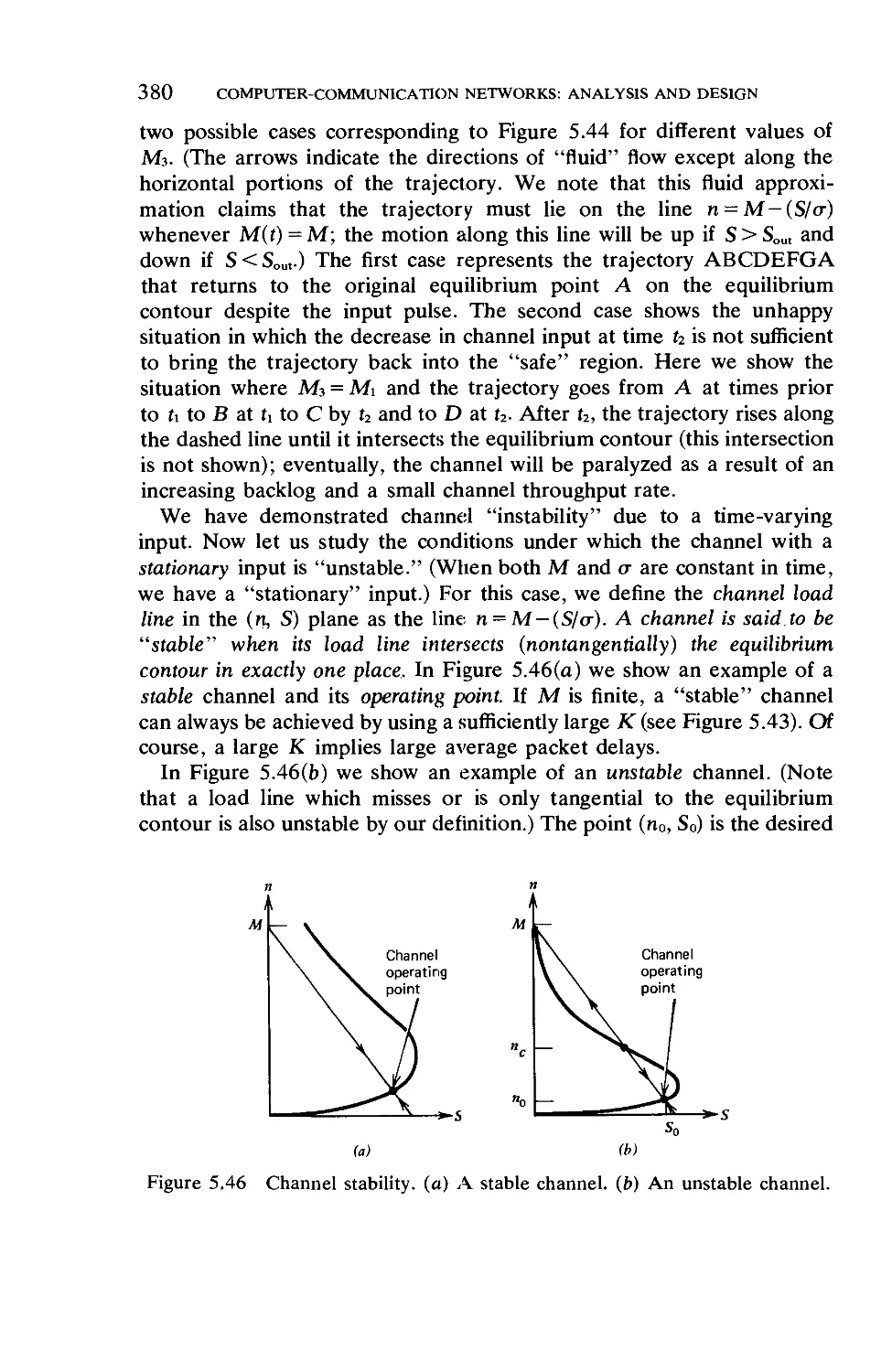
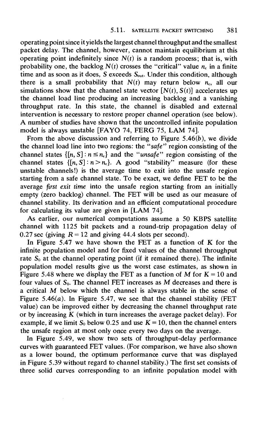
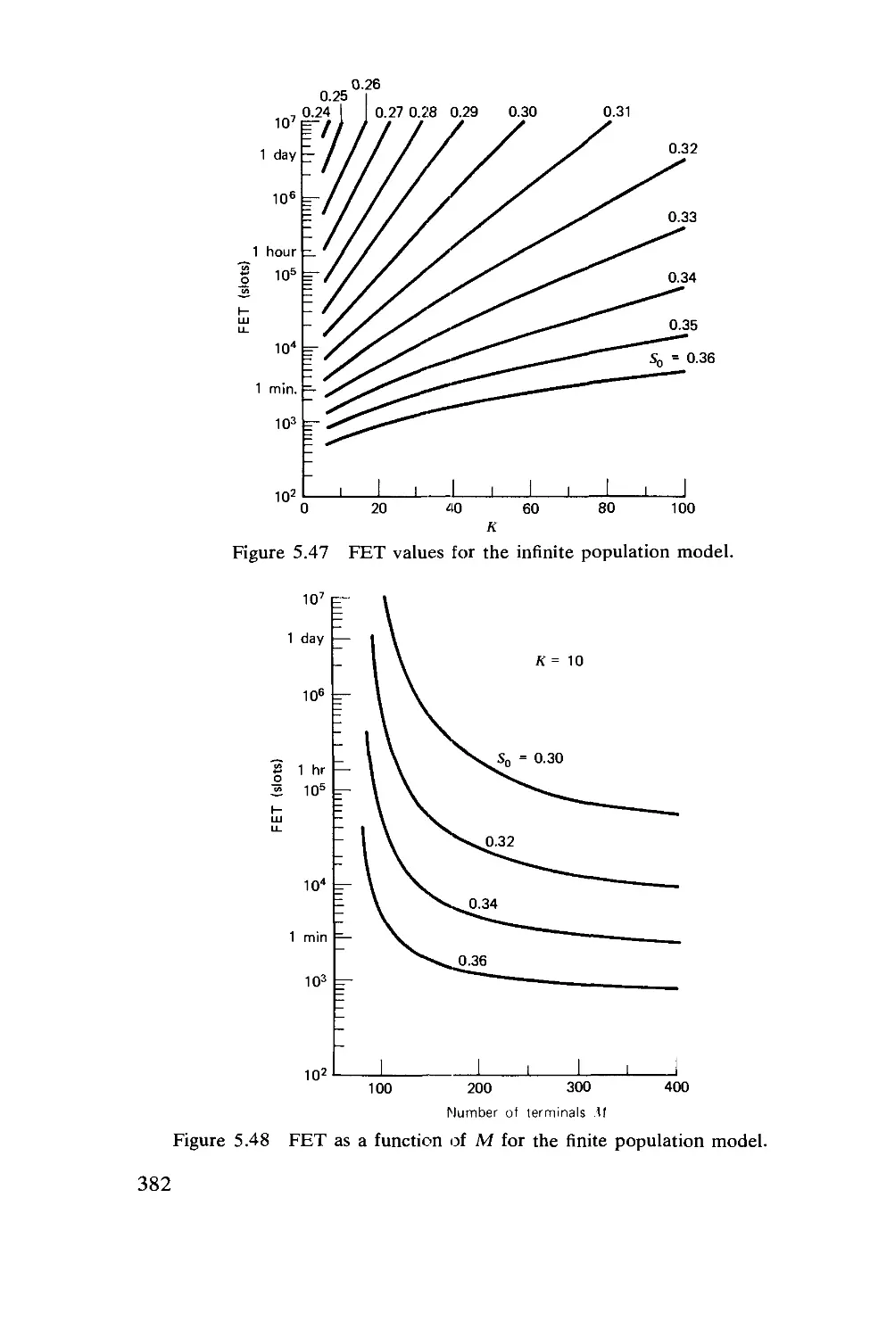
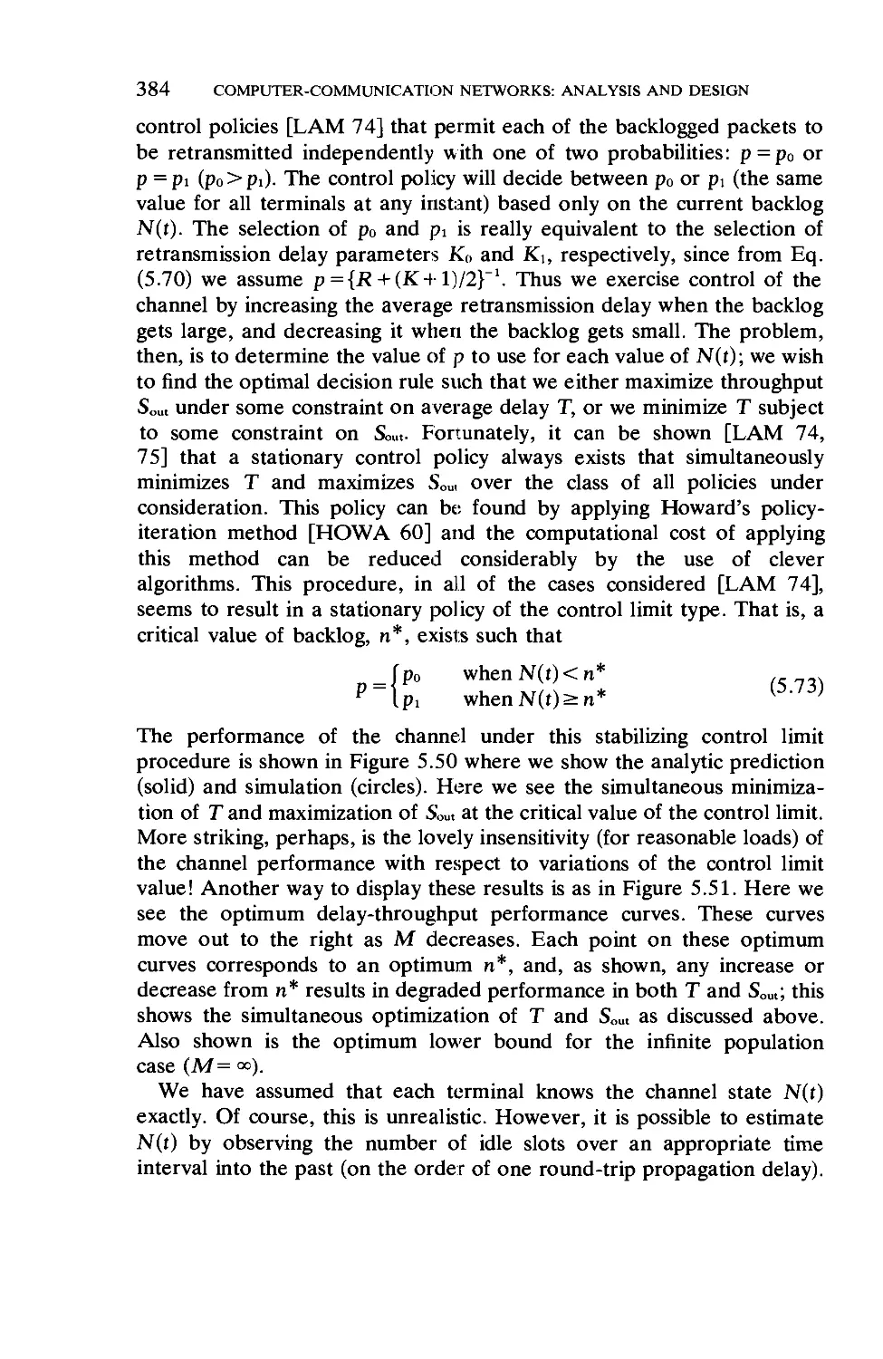
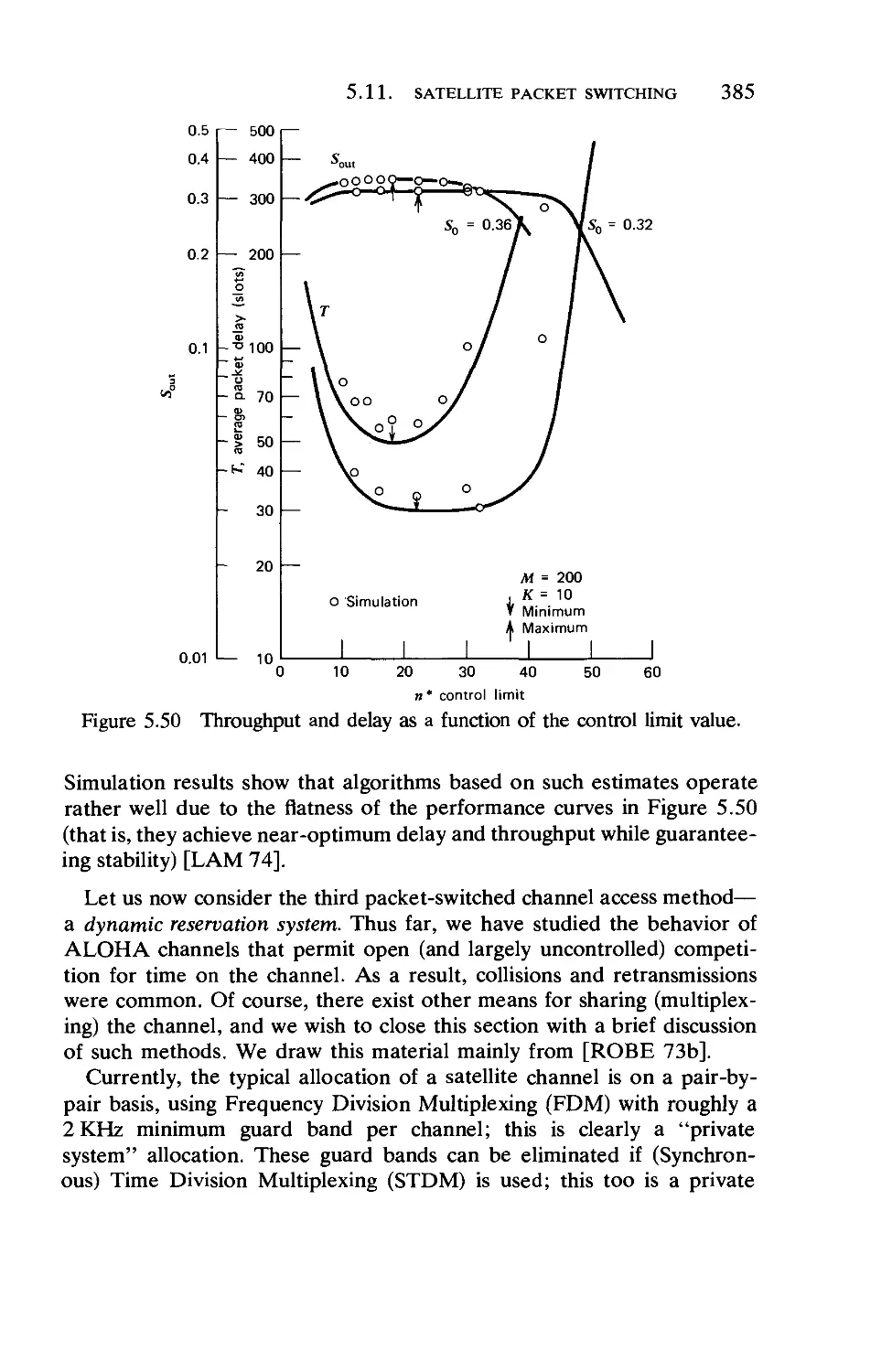
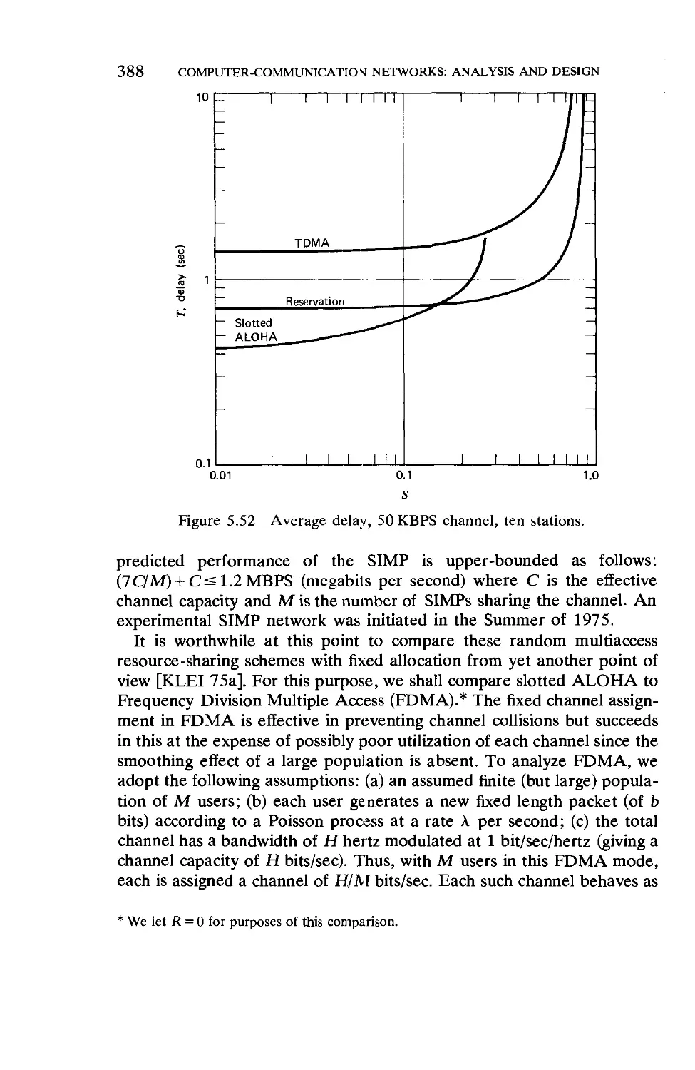
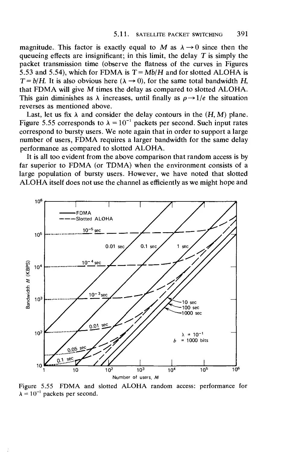
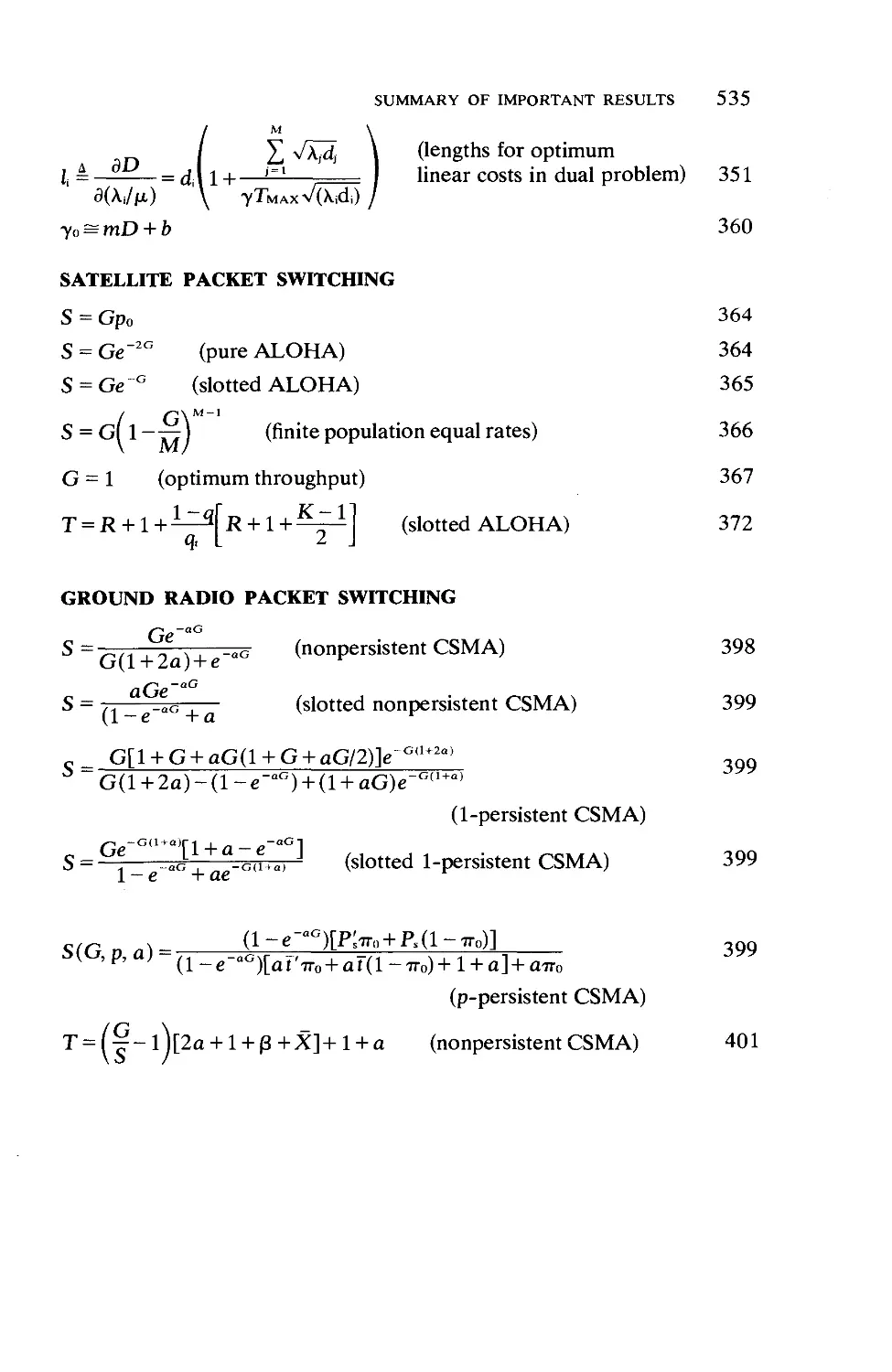
5.11. Satellite Packet Switching ....
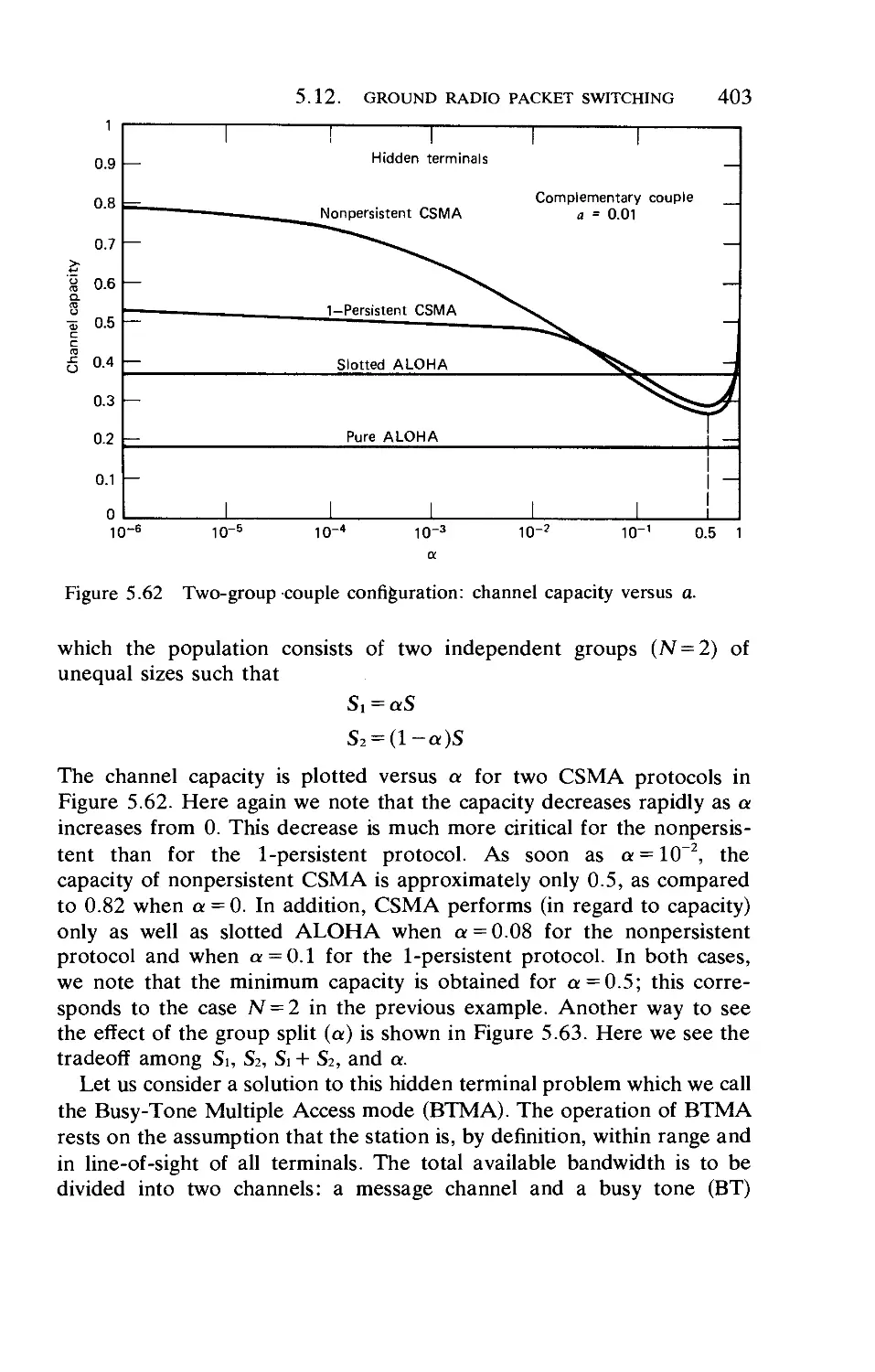
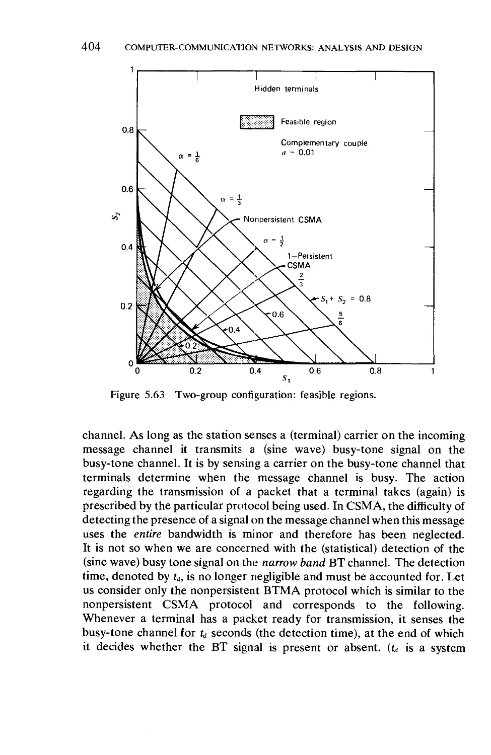
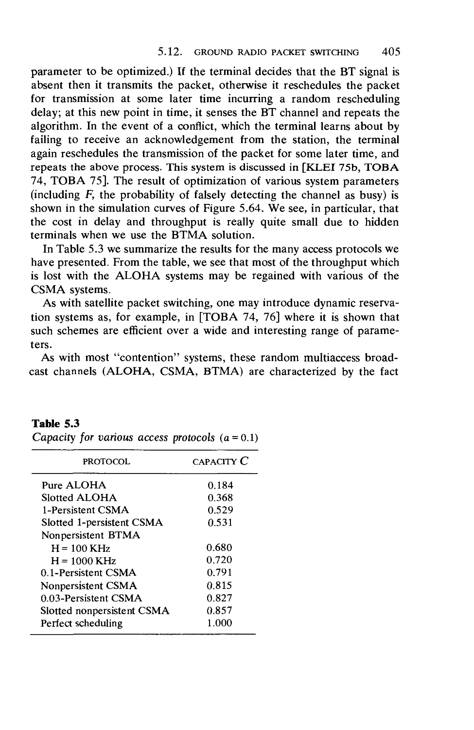
5.12. Ground Radio Packet Switching.
113
118
119
126
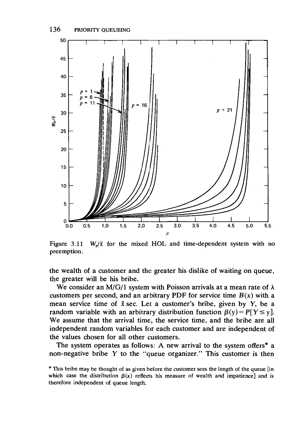
135
144
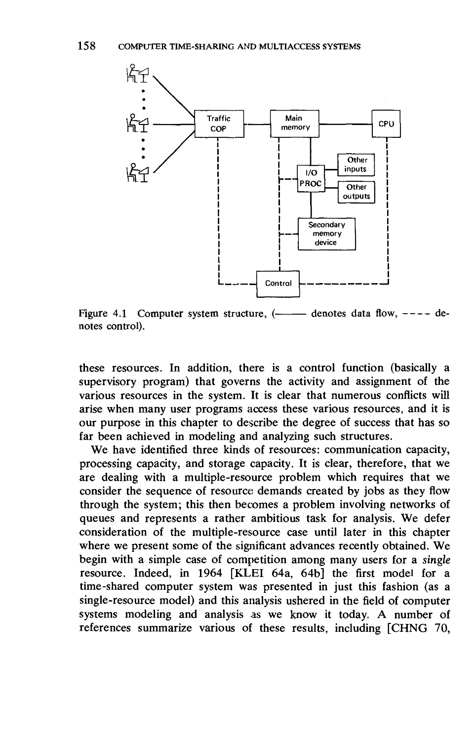
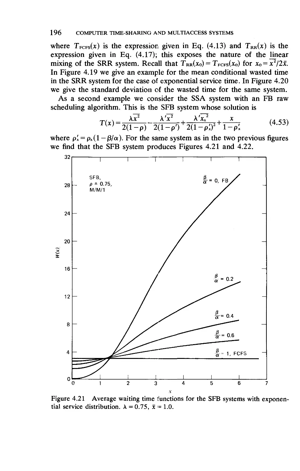
Chapter 4 Computer Time-Sharing and Multiaccess Systems 156
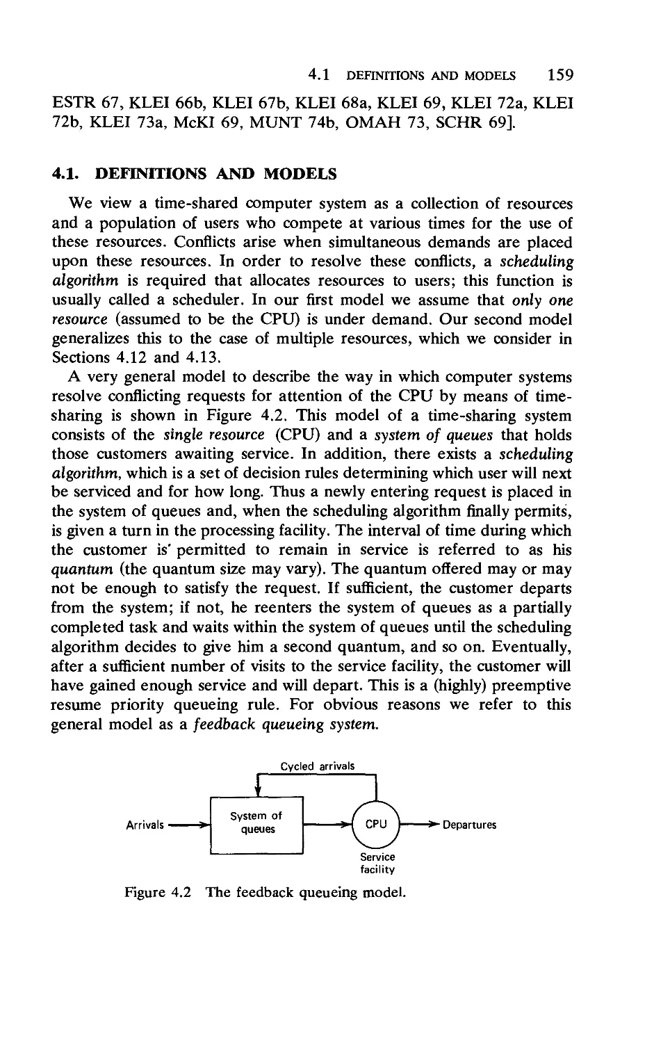
4.1. Definitions and Models 159
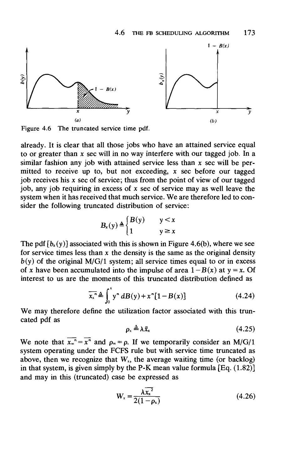
4.2. Distribution of Attained Service 162
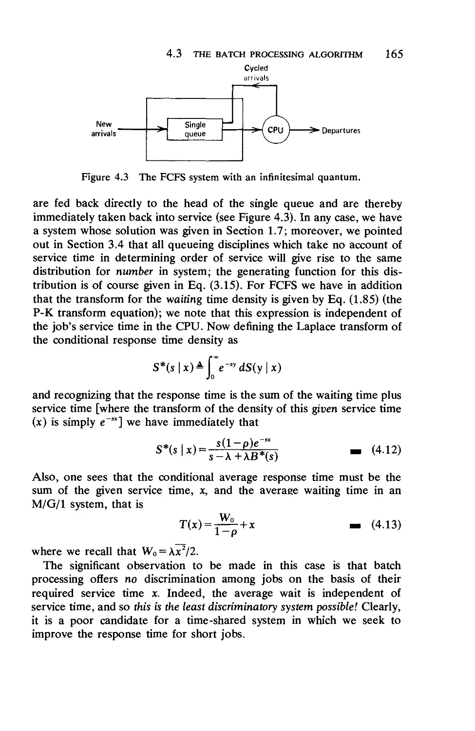
4.3. The Batch Processing Algorithm 164
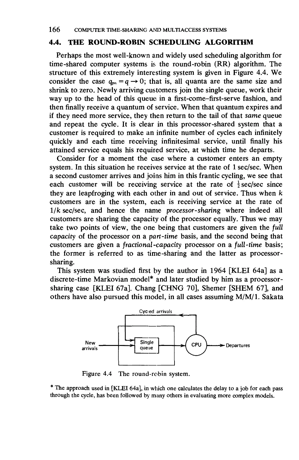
4.4. The Round-Robin Scheduling Algorithm . 166
4.5. The Last-Come-First-Serve Scheduling Algorithm . 170
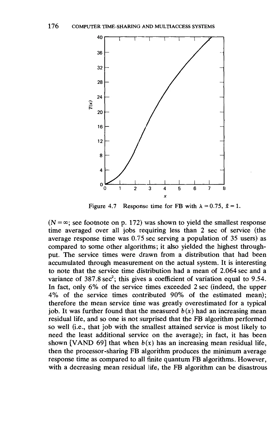
4.6. The FB Scheduling Algorithm 172
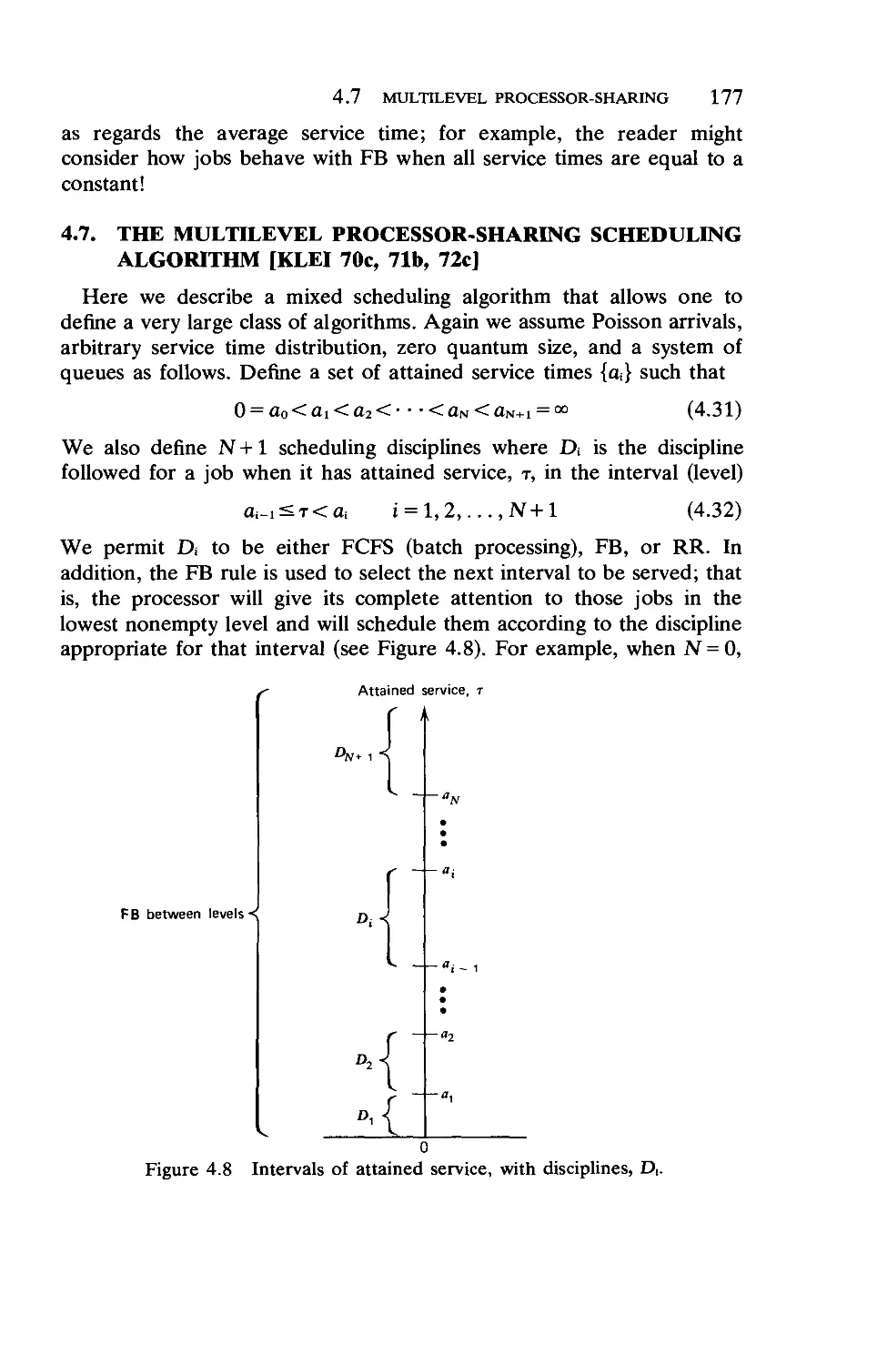
4.7. The Multilevel Processor Sharing Scheduling
Algorithm 177
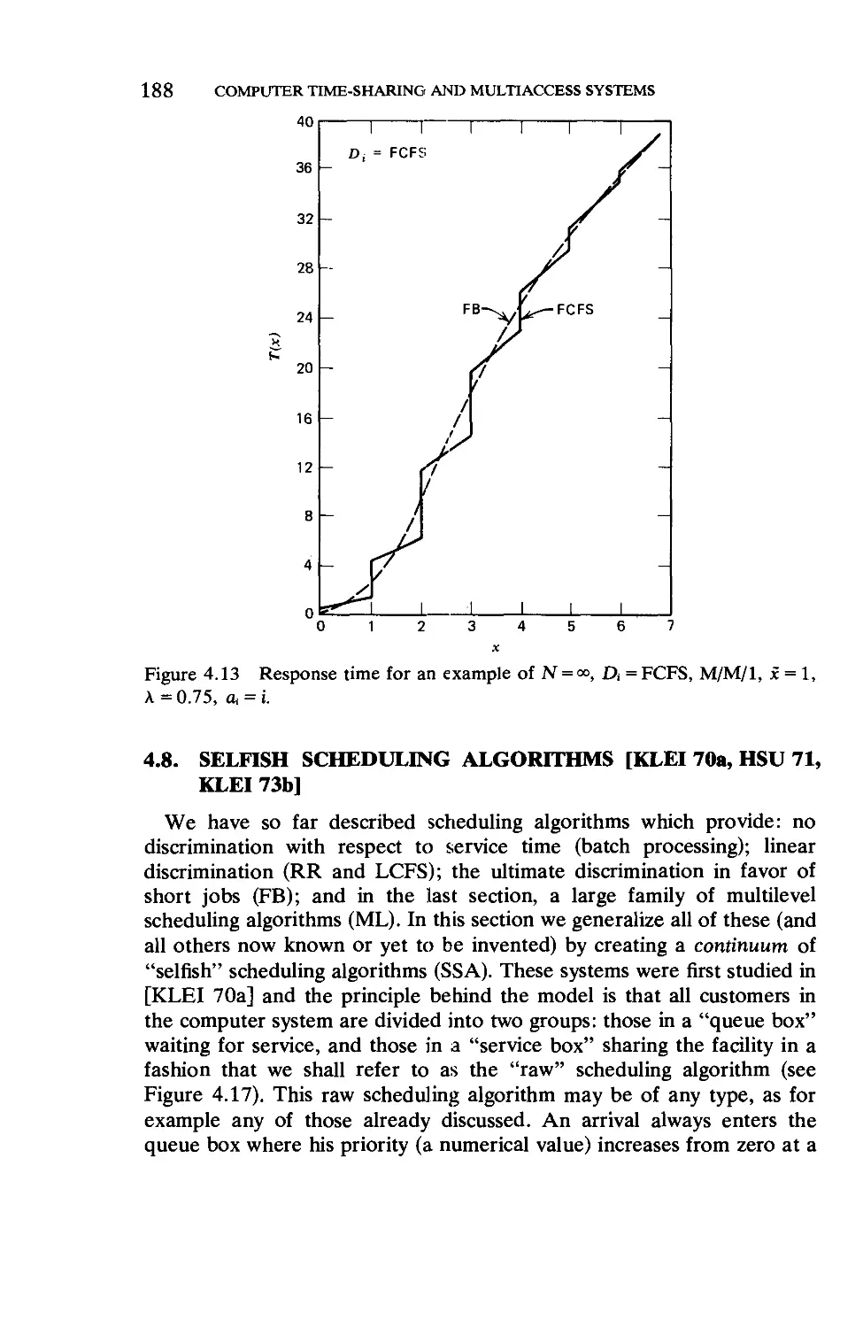
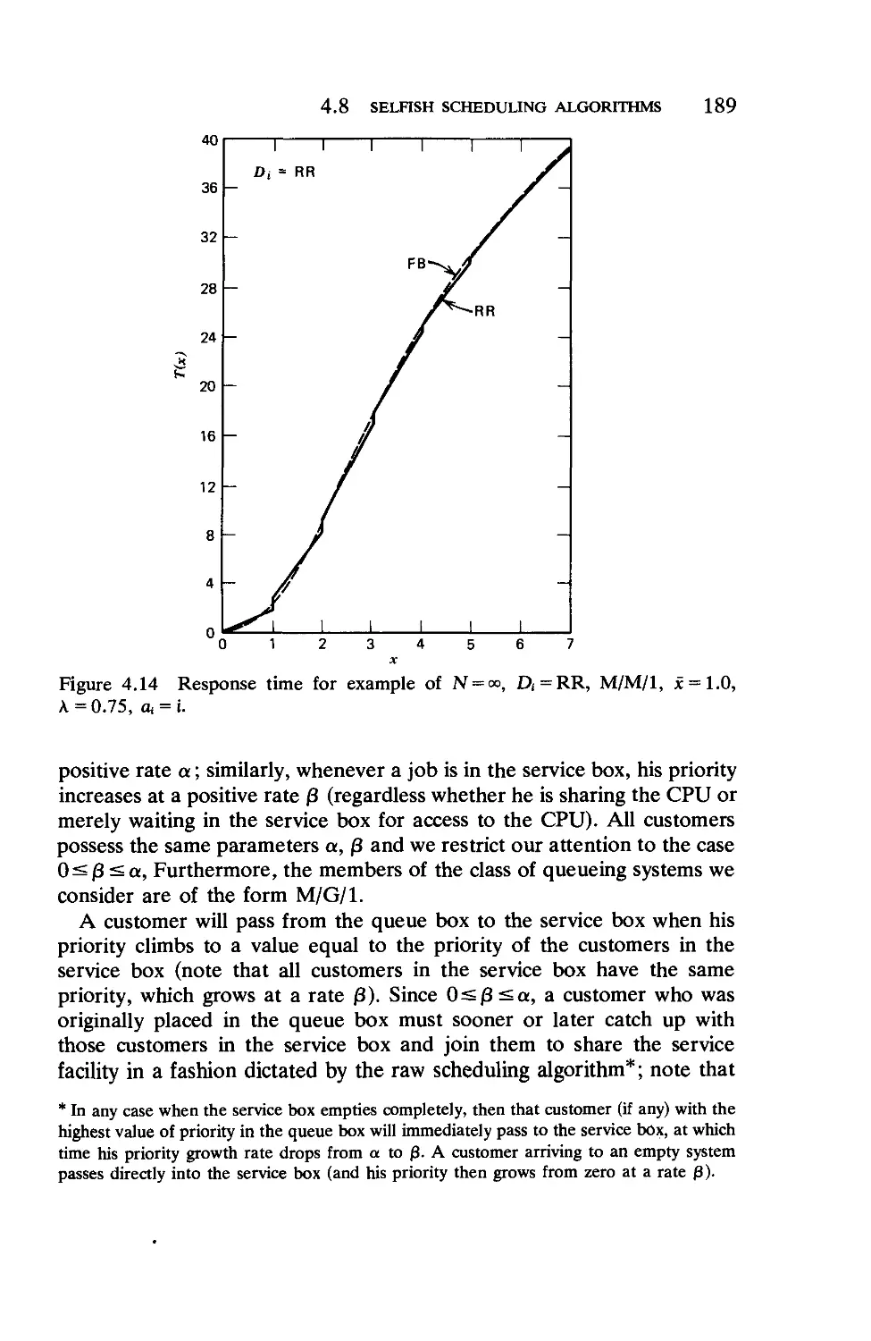
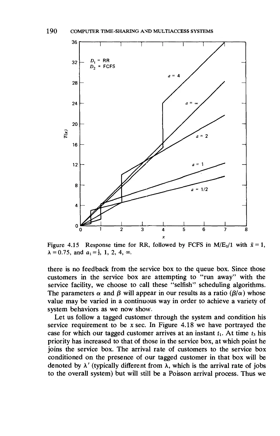
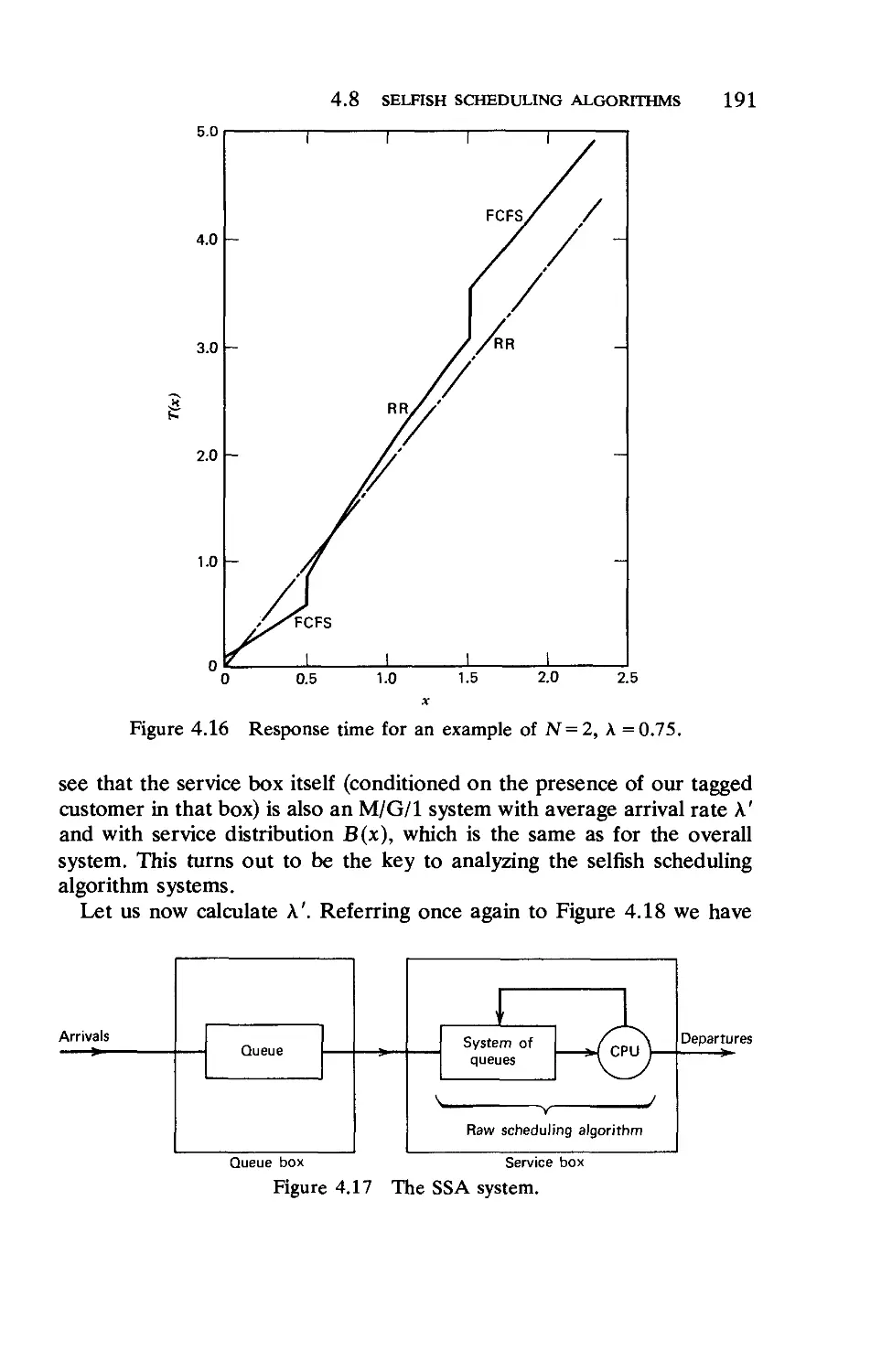
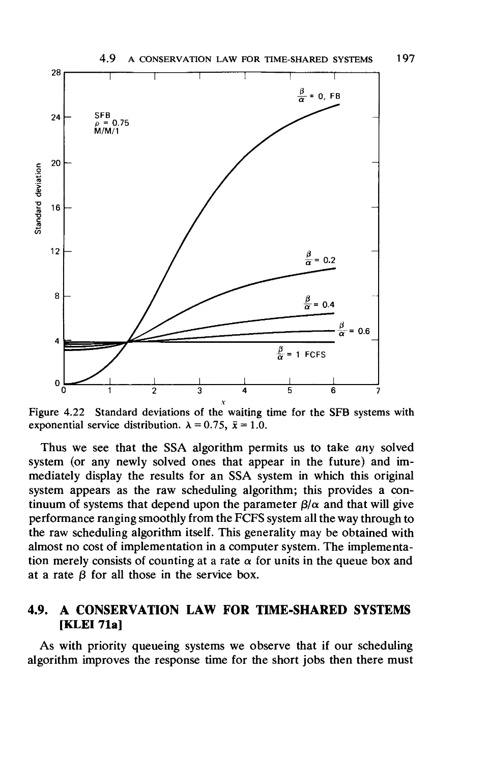
4.8. Selfish Scheduling Algorithms 188
4.9. A Conservation Law for Time-Shared Systems . . 197
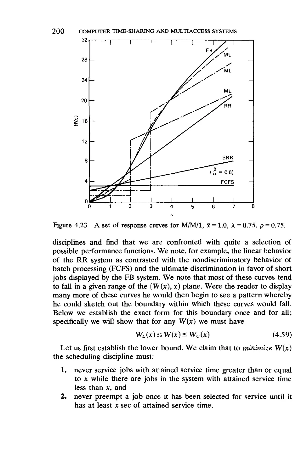
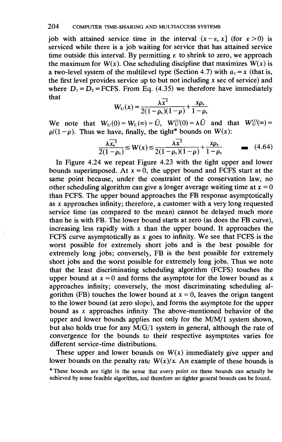
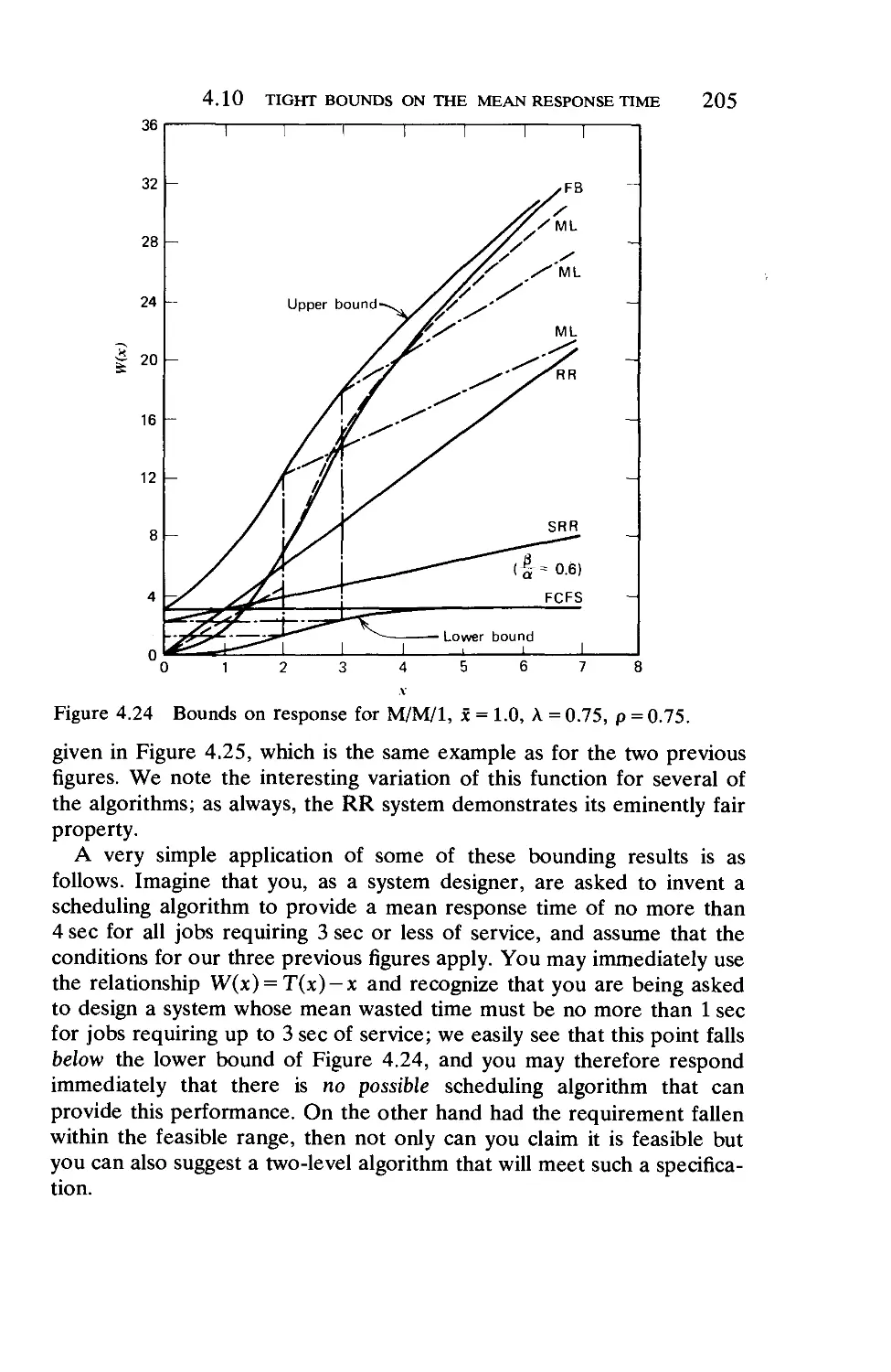
4.10. Tight Bounds on the Mean Response Time . . 199
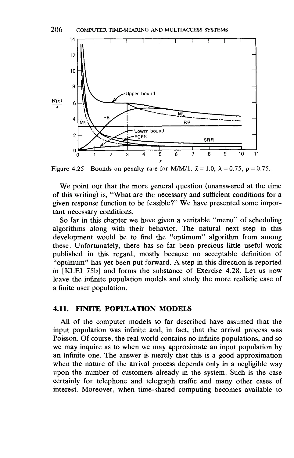
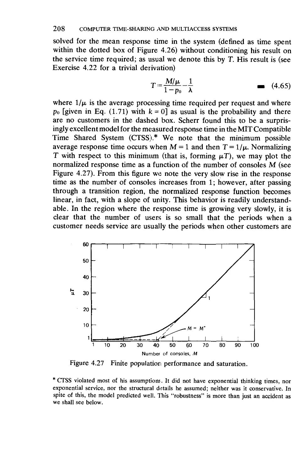
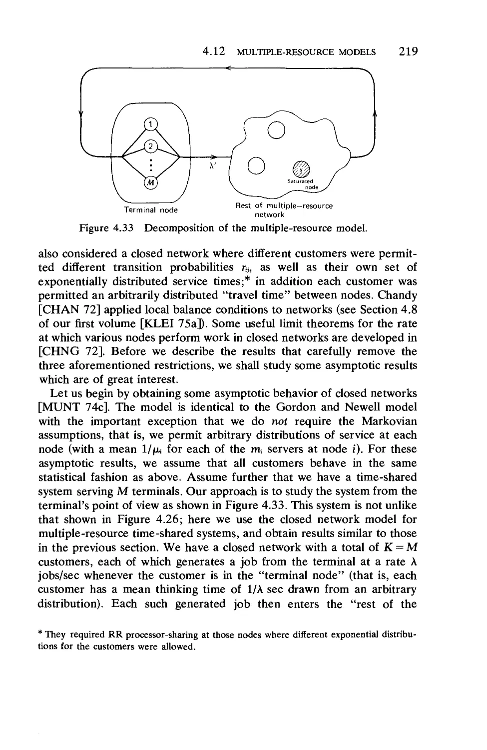
4.11. Finite Population Models 206
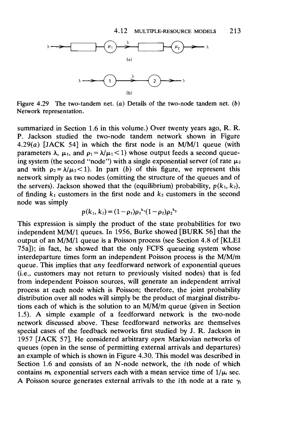
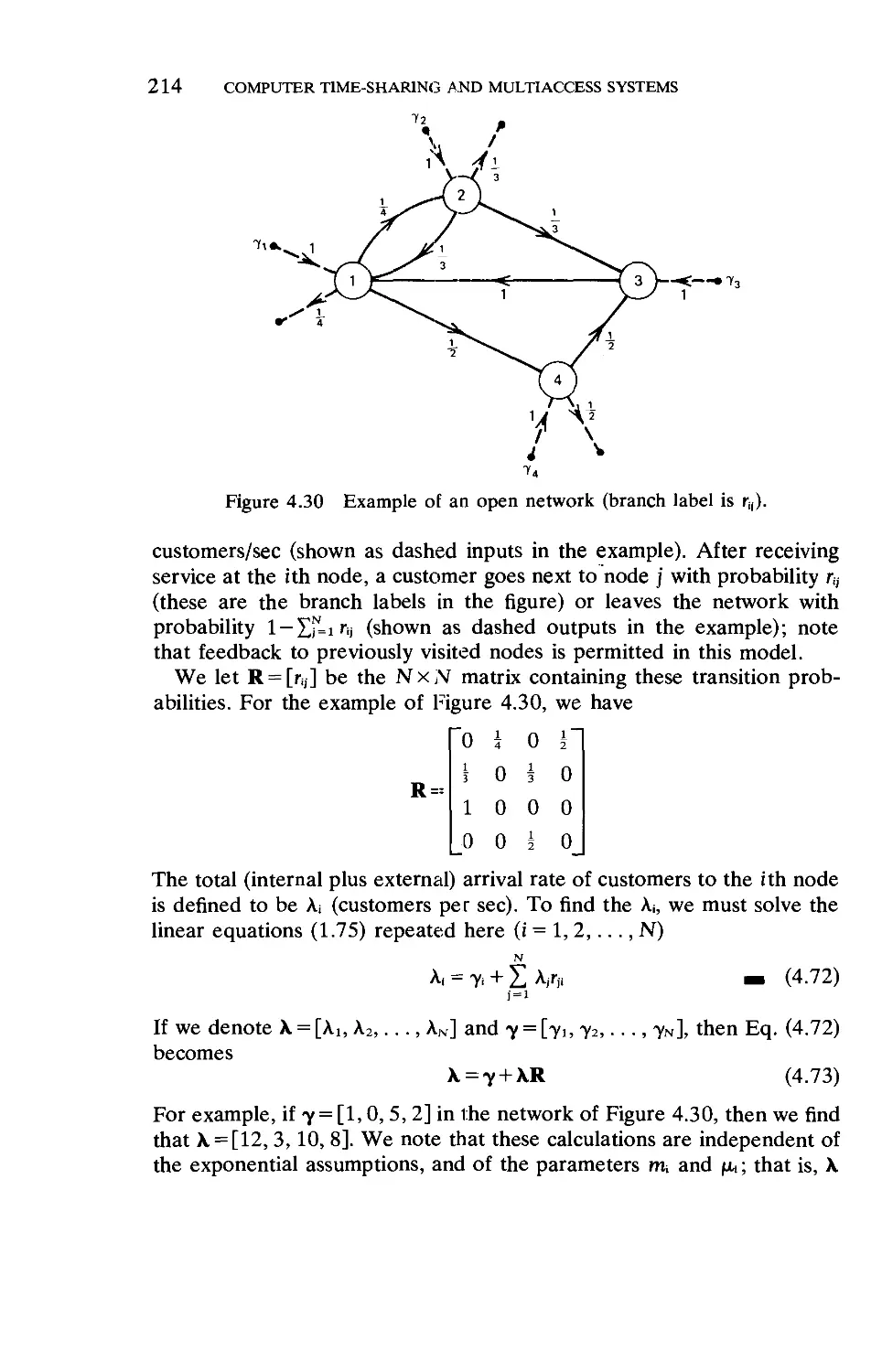
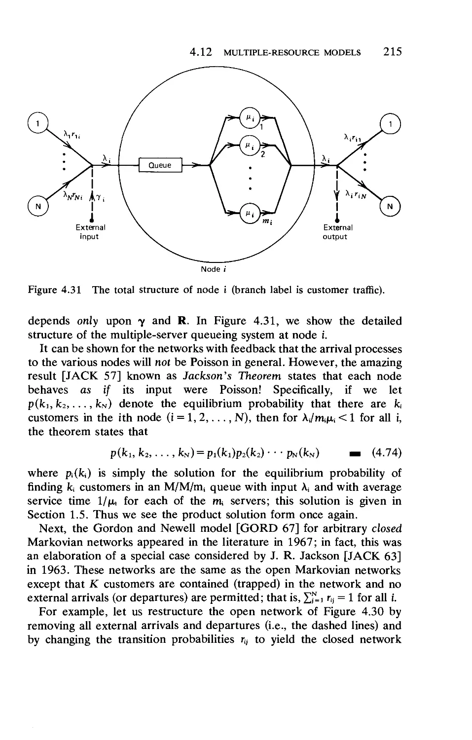
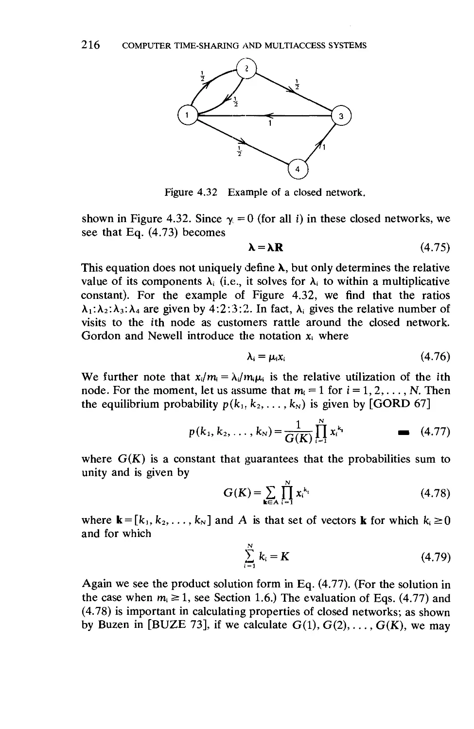
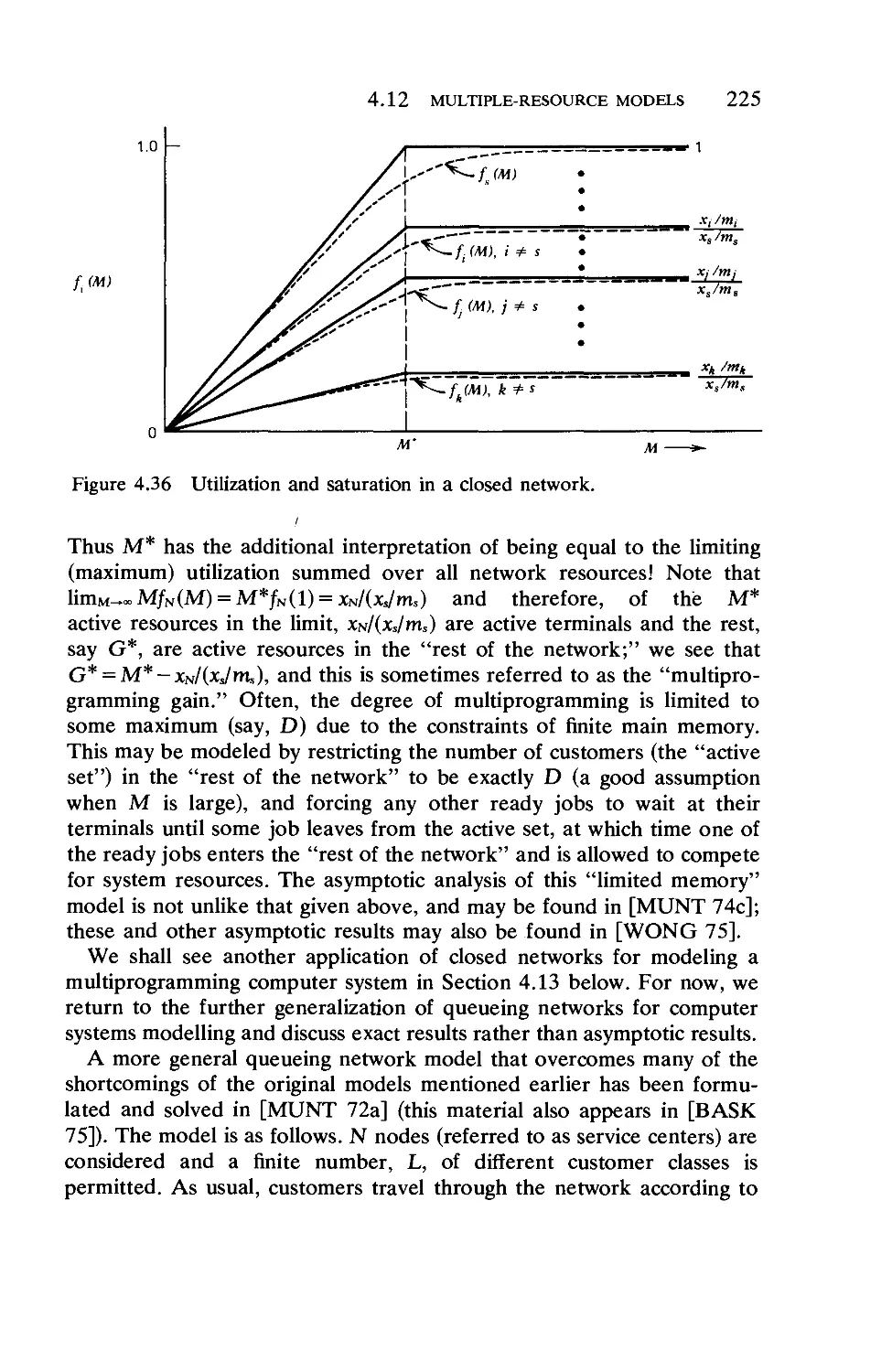
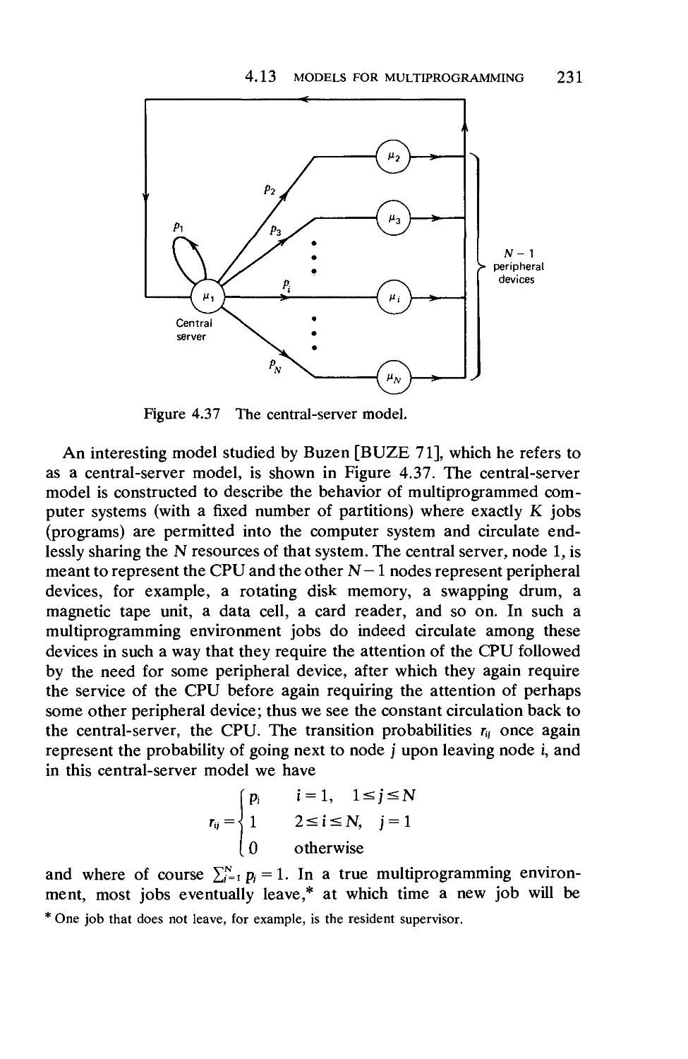
4.12. Multiple-Resource Models 212
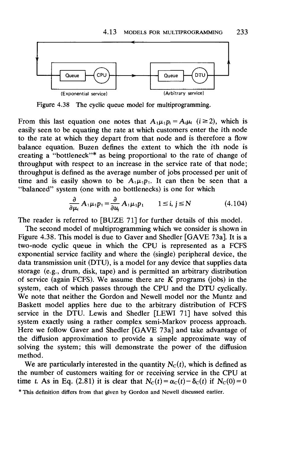
4.13. Models for Multiprogramming 230
4.14. Remote Terminal Access to Computers . 236
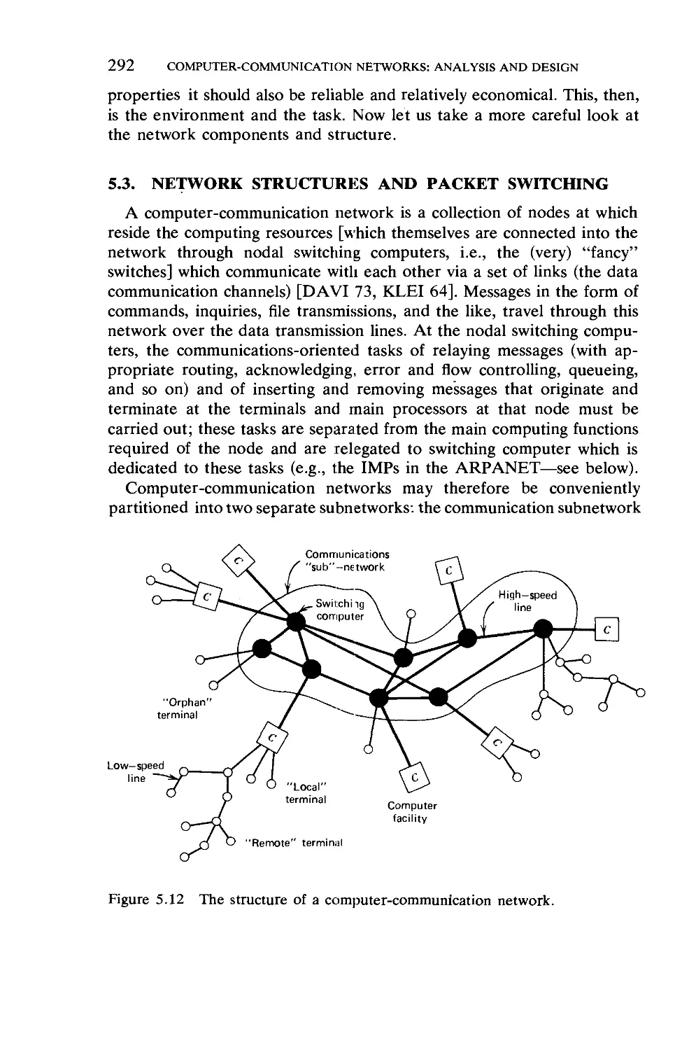
Chapter 5 Computer-Communication Networks: Analysis and
Design 270
272
290
. 292
of an
. 304
314
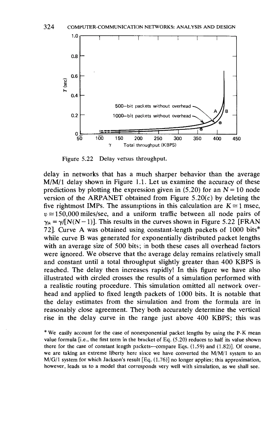
. 320
. 329
340
. 348
to the
351
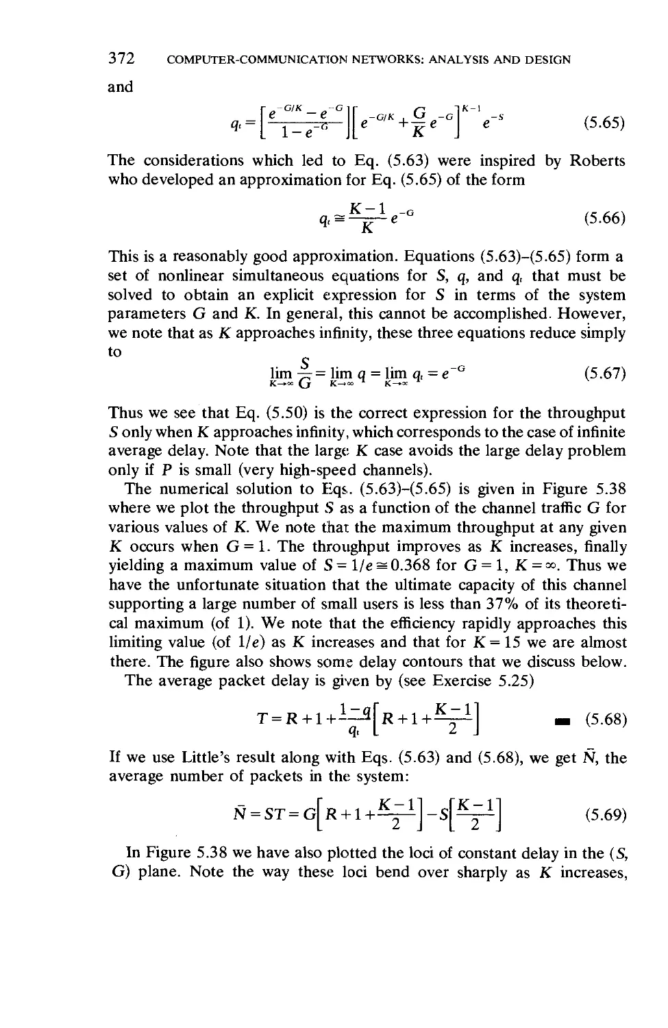
. 360
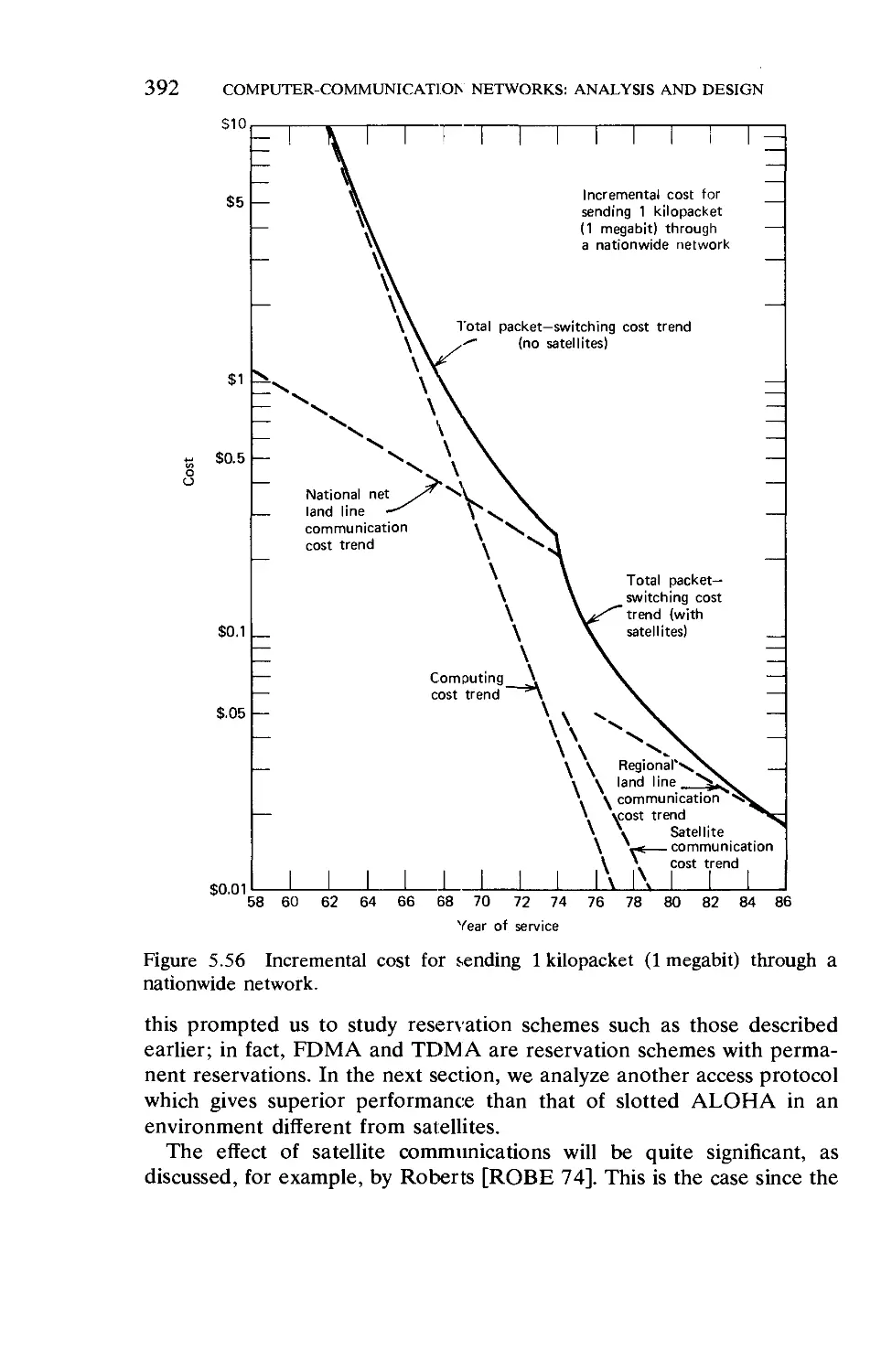
. 393
CONTENTS
XV11
Chapter 6 Computer-Communication Networks: Measurement,
Flow Control, and ARPANET Traps
6.1.
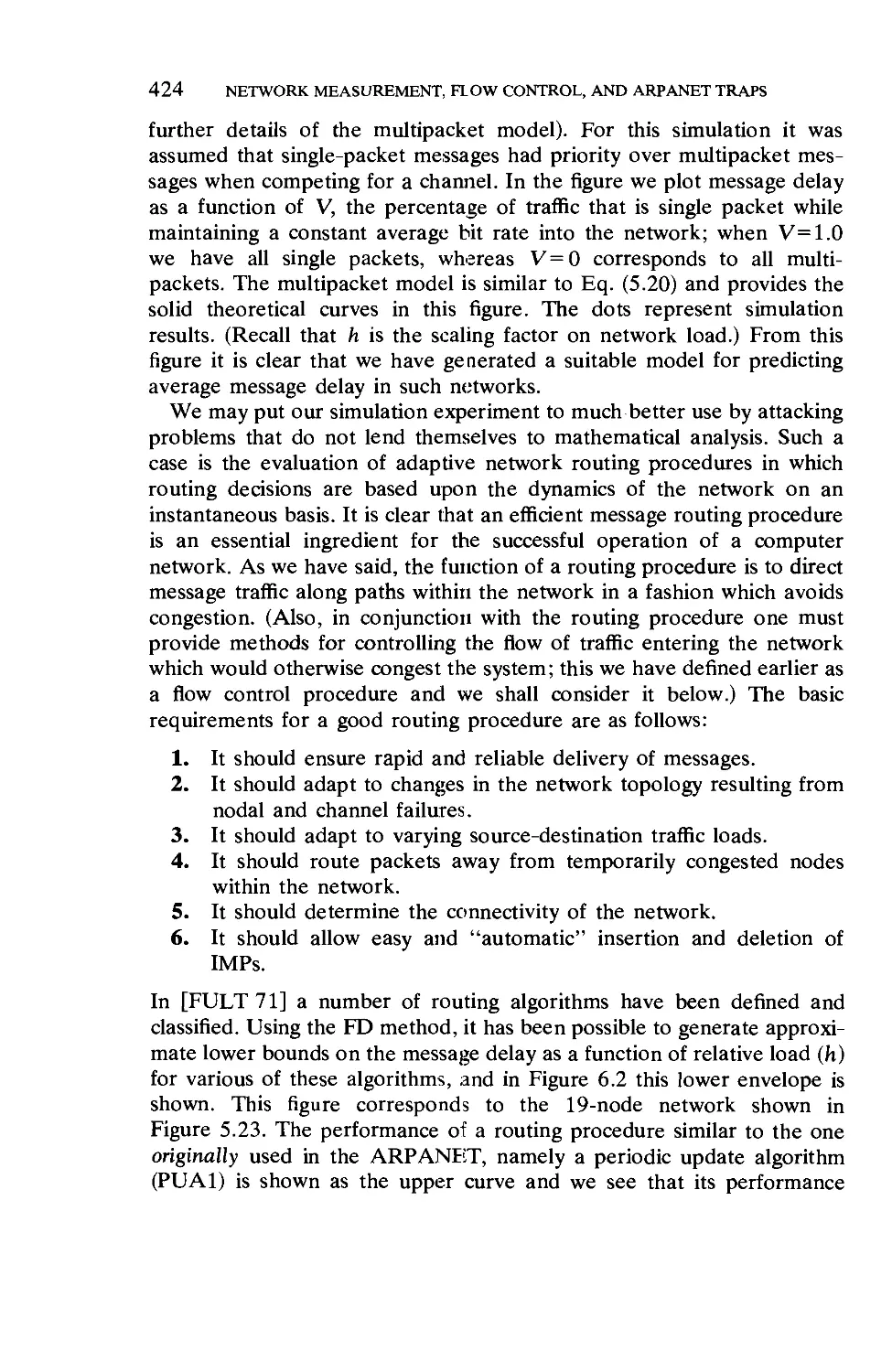
6.2.
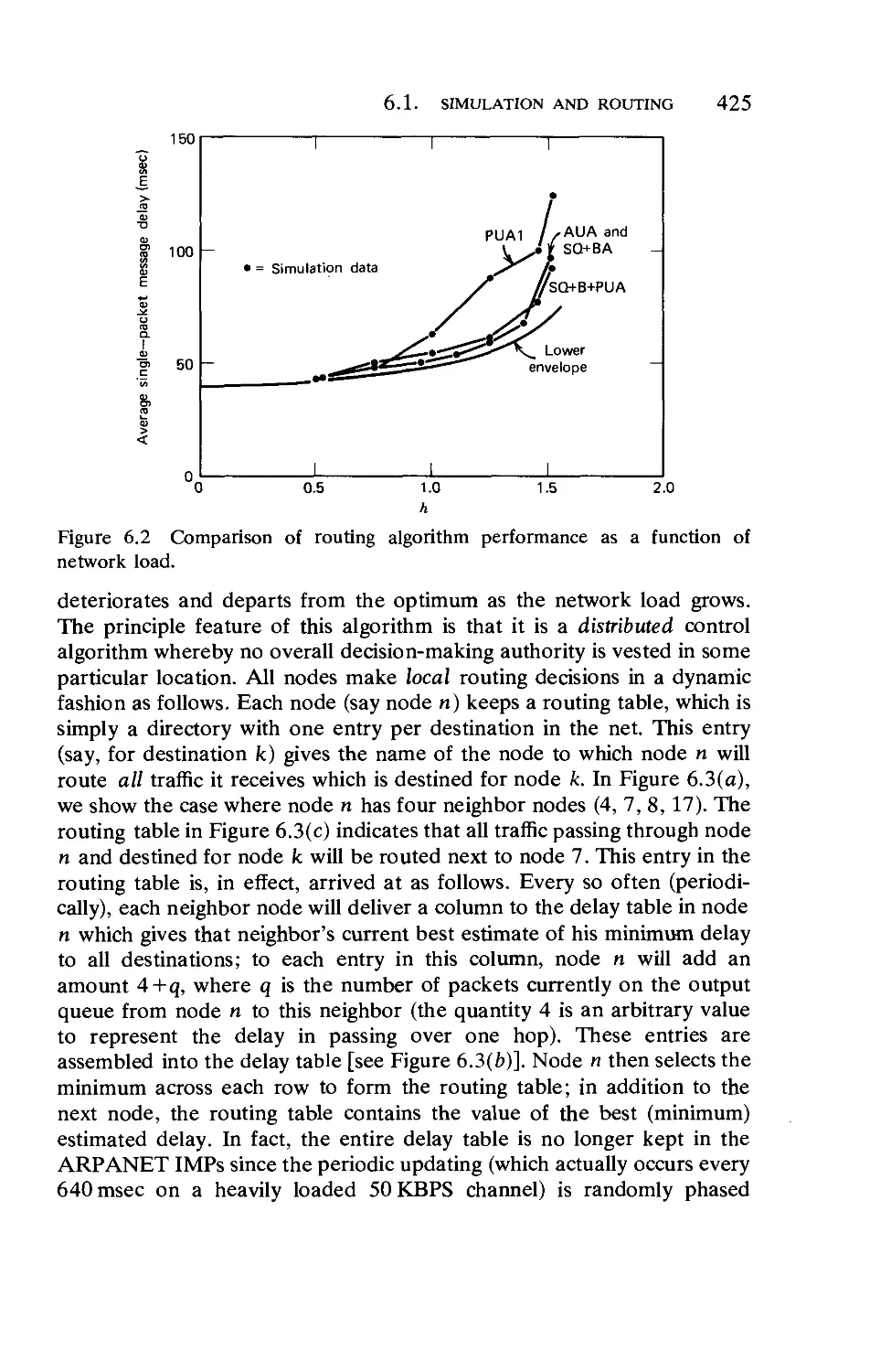
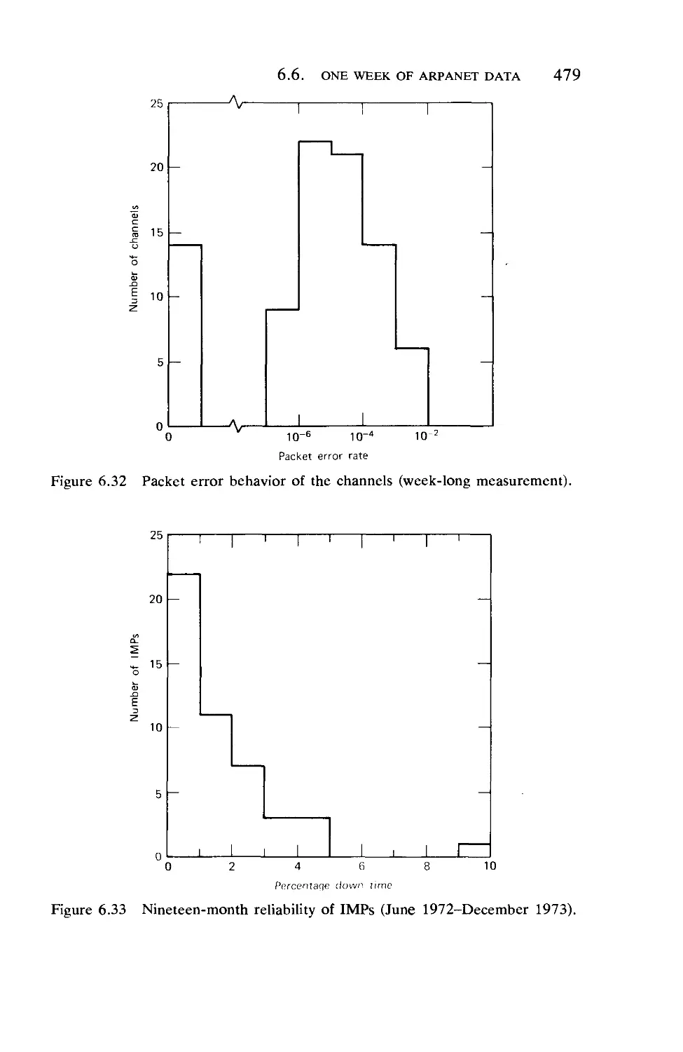
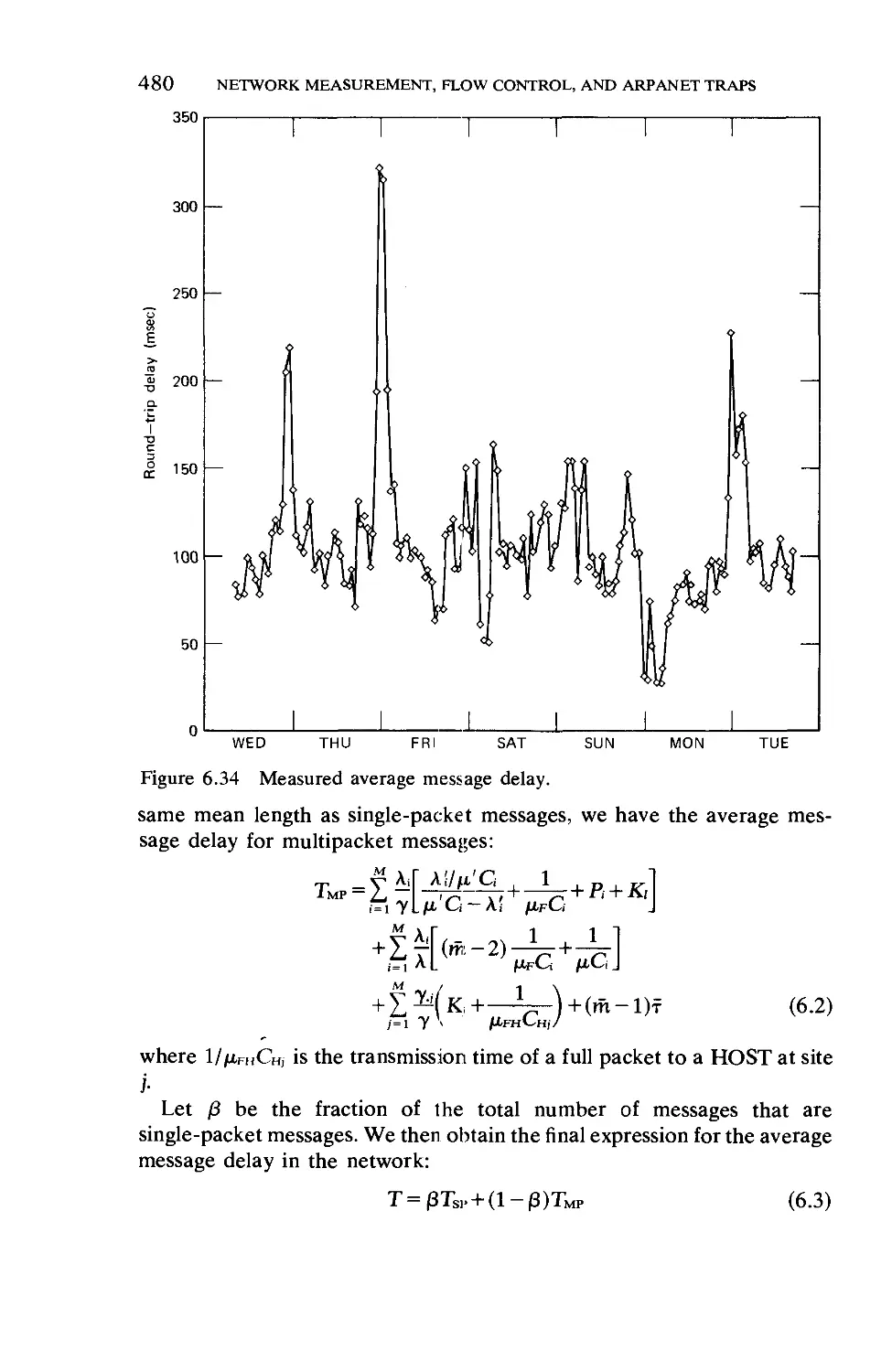
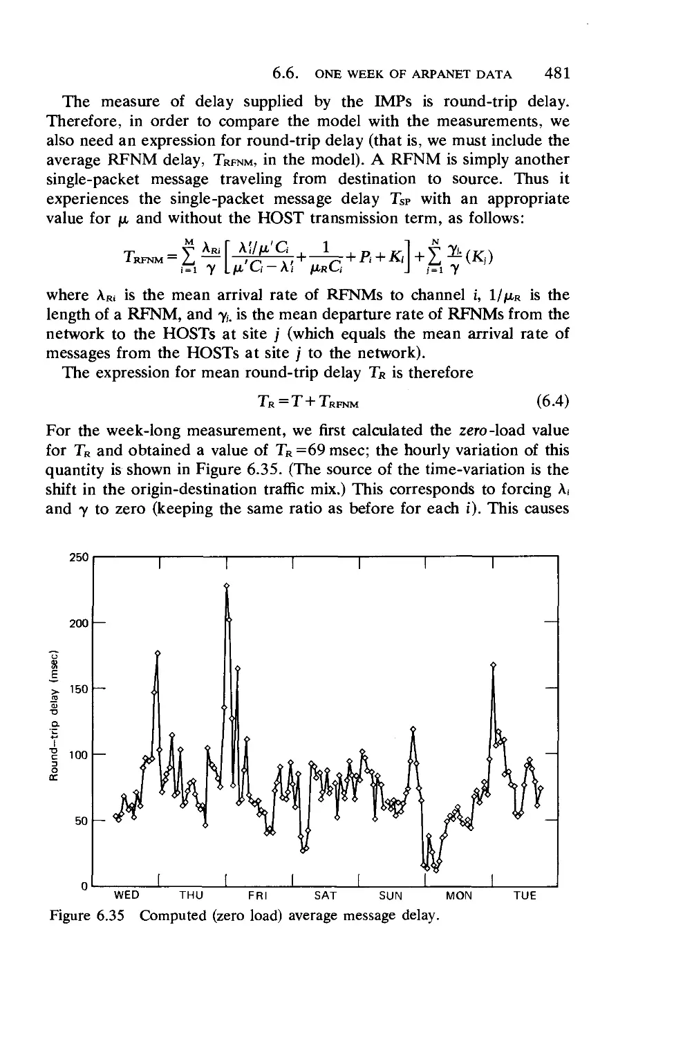
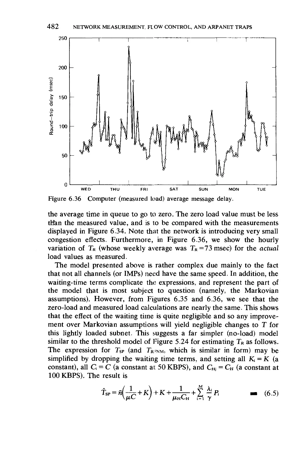
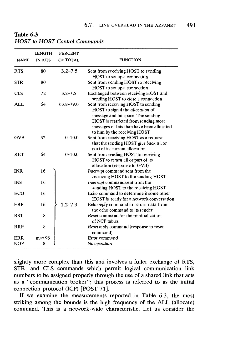
6.3.
6.4.
6.5.
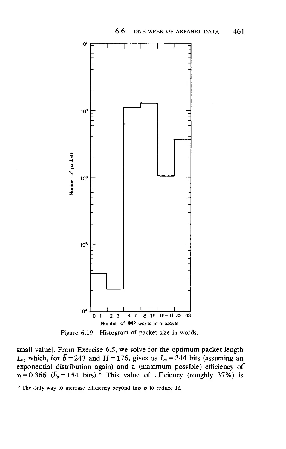
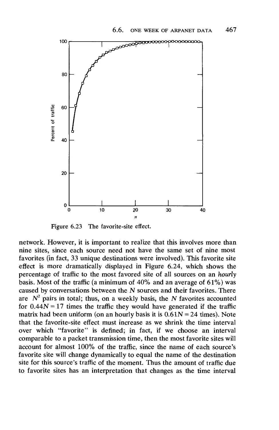
6.6.
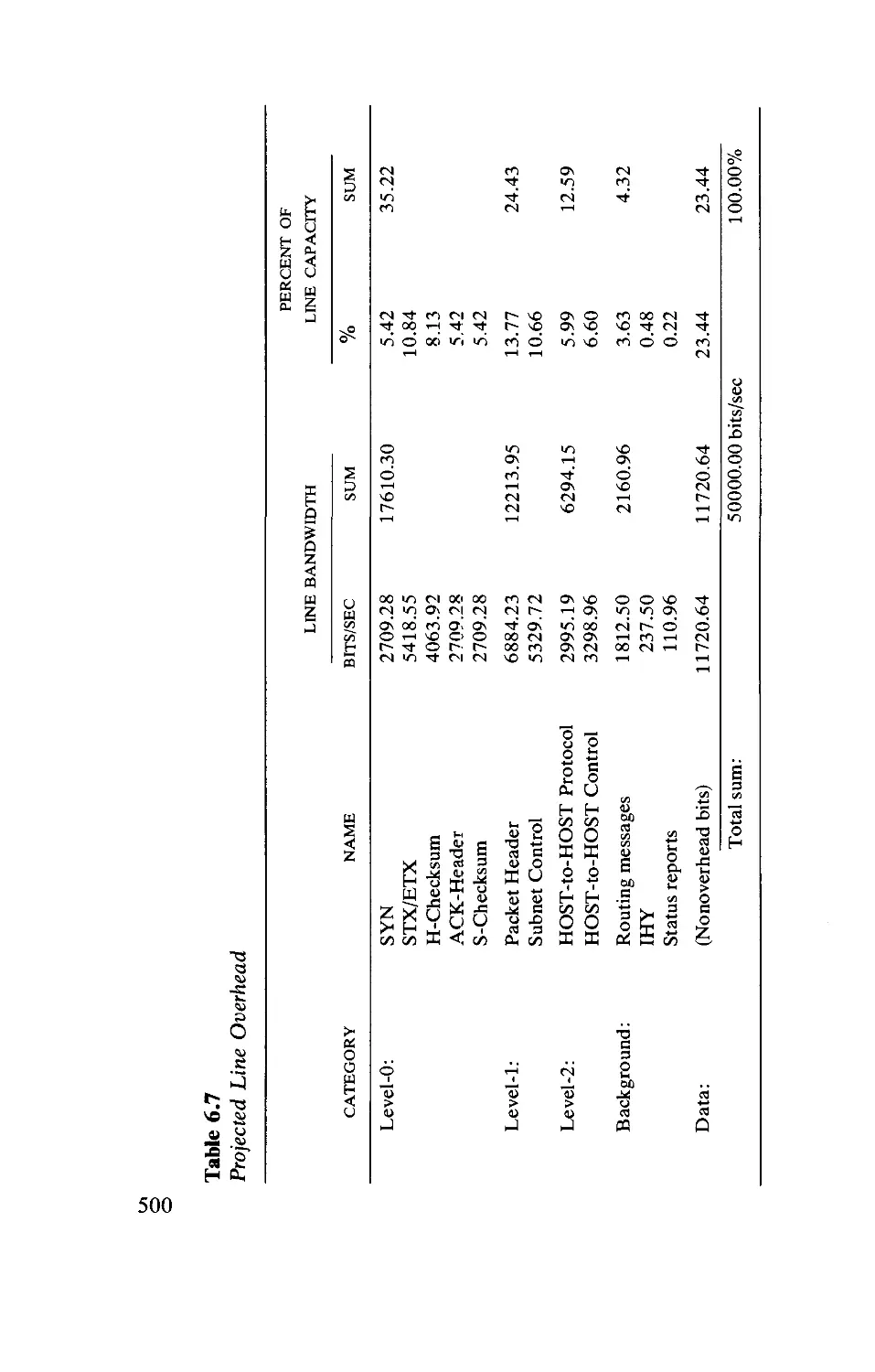
6.7.
6.8.
6.9.
Simulation and Routing
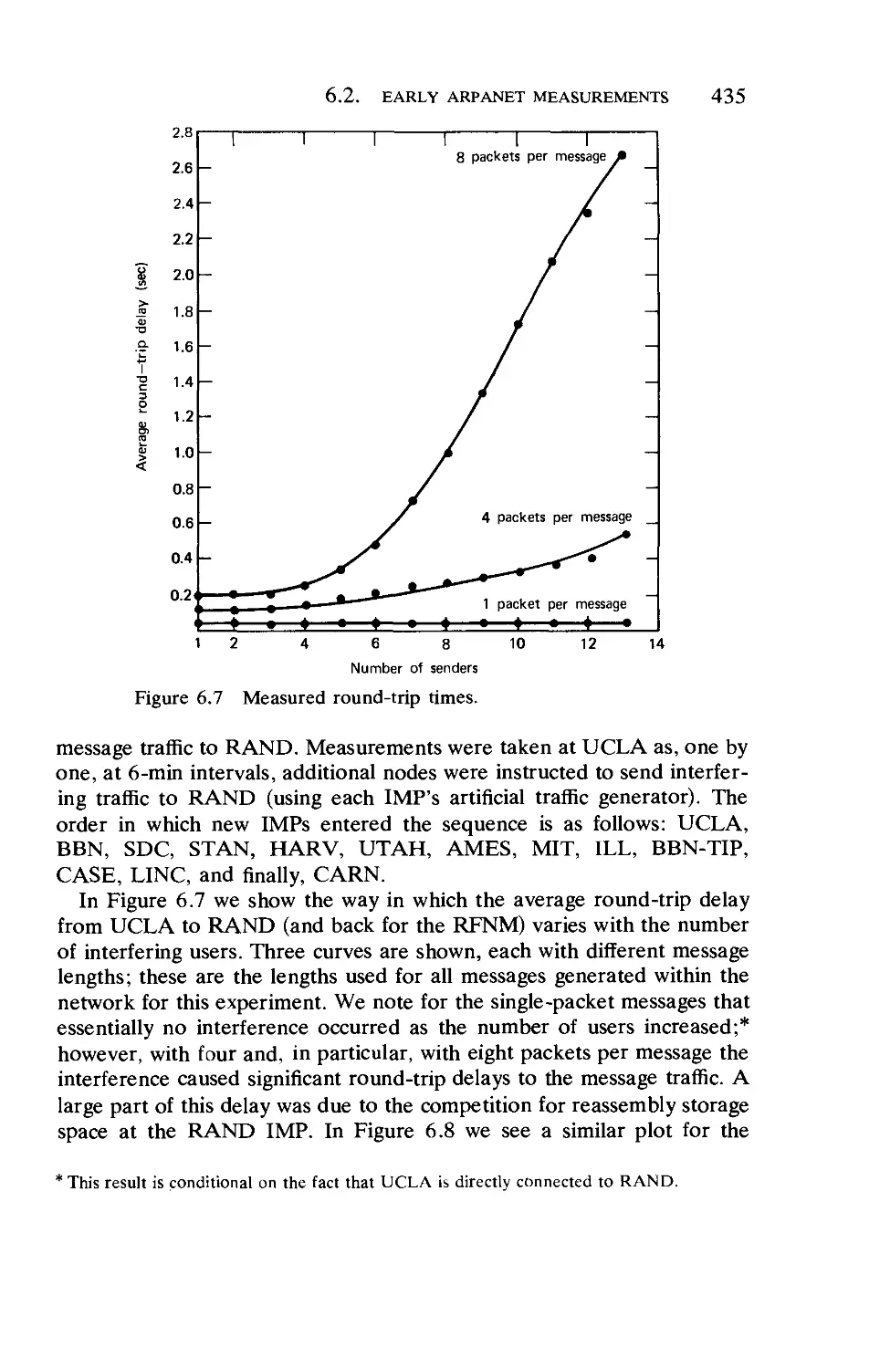
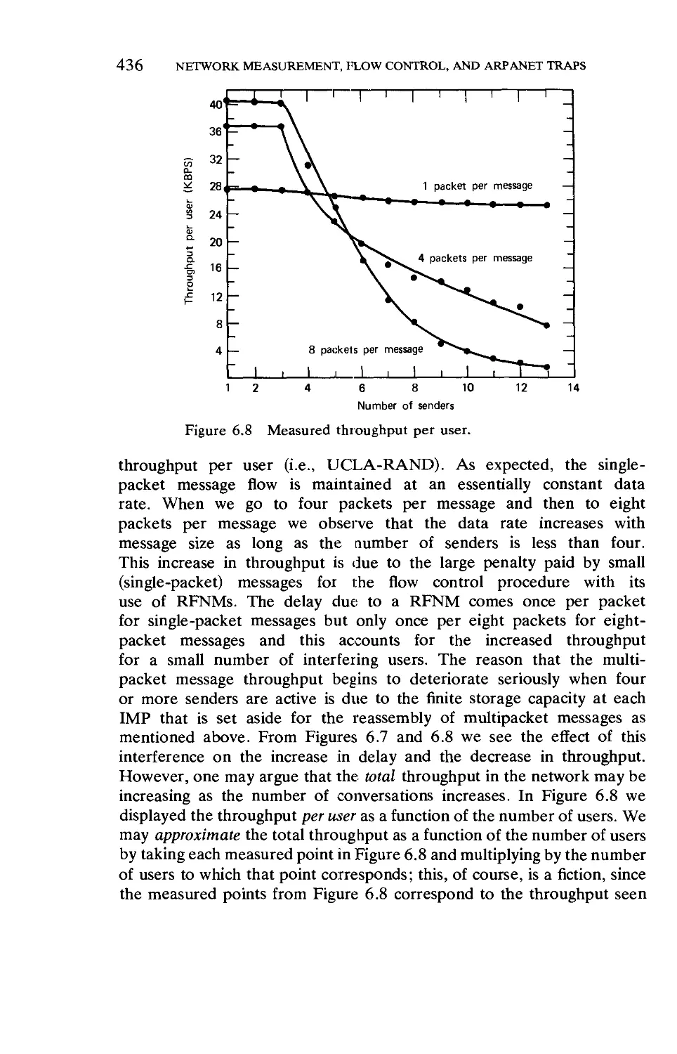
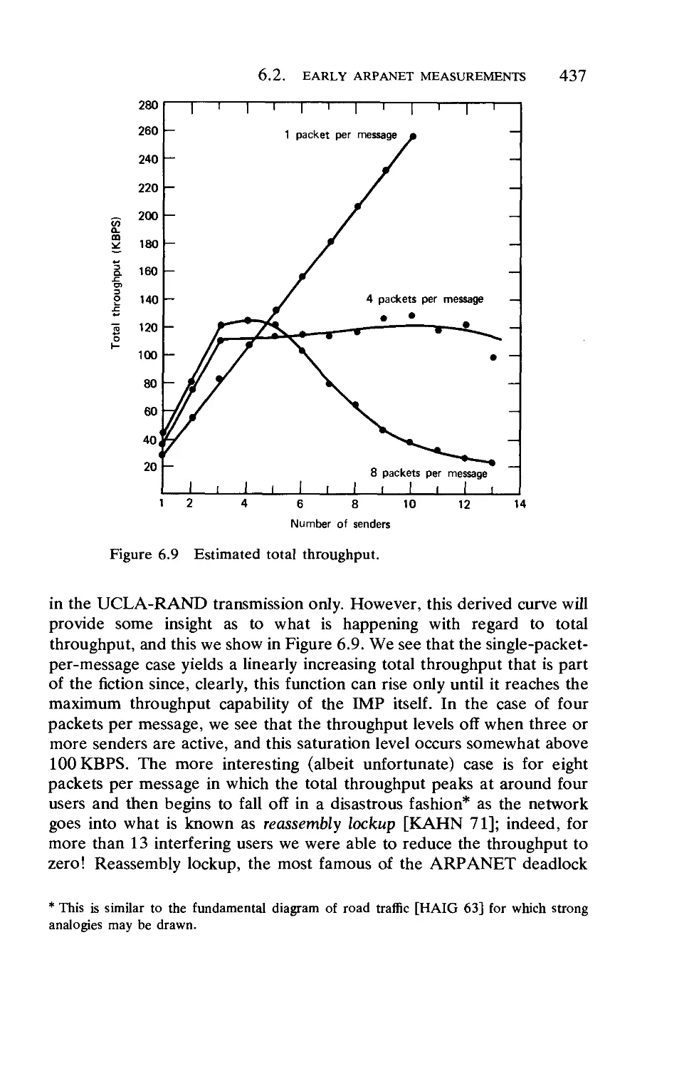
Early ARPANET Measurements
Flow Control
Lockups, Degradations, and Traps . . .
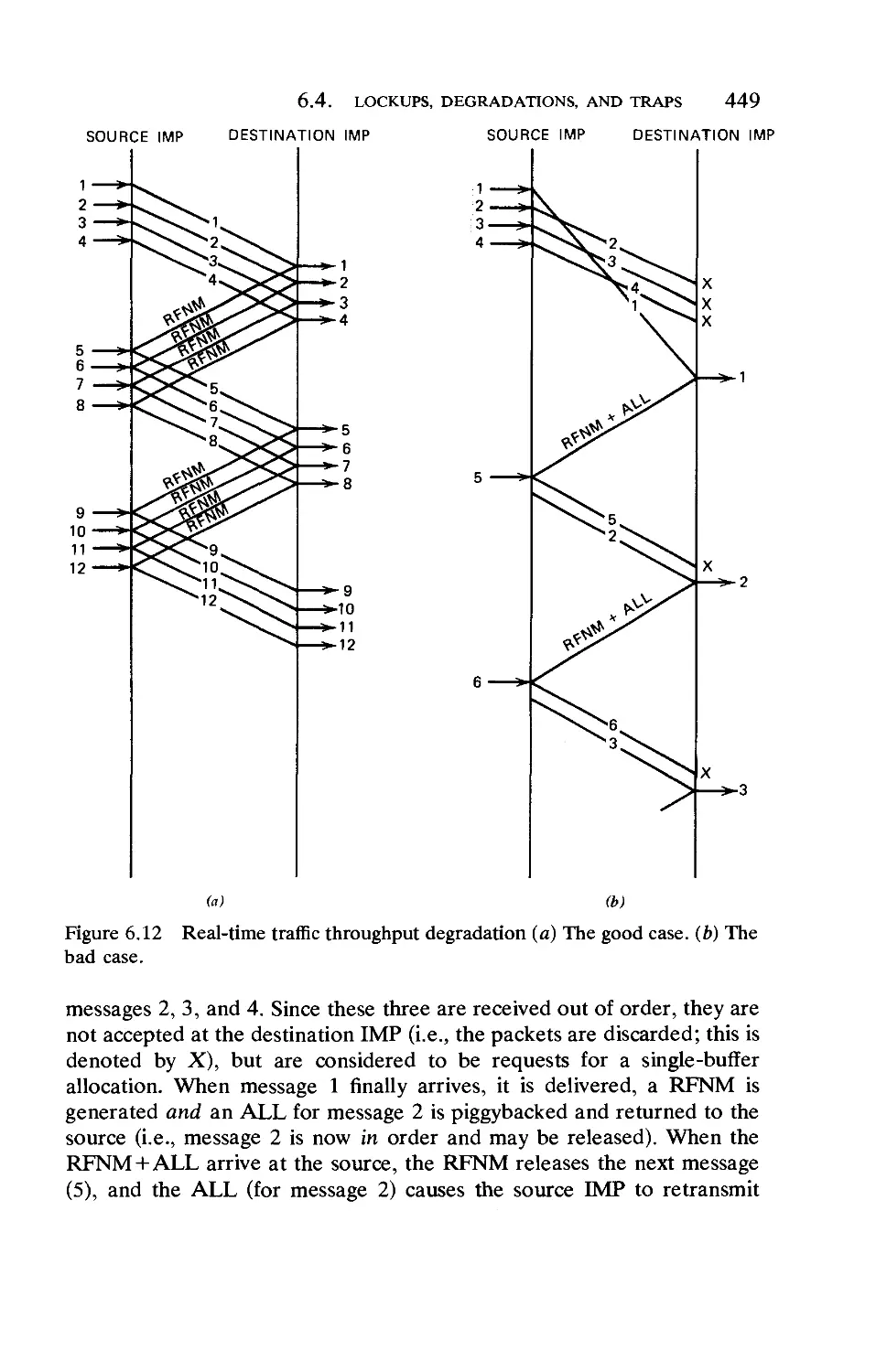
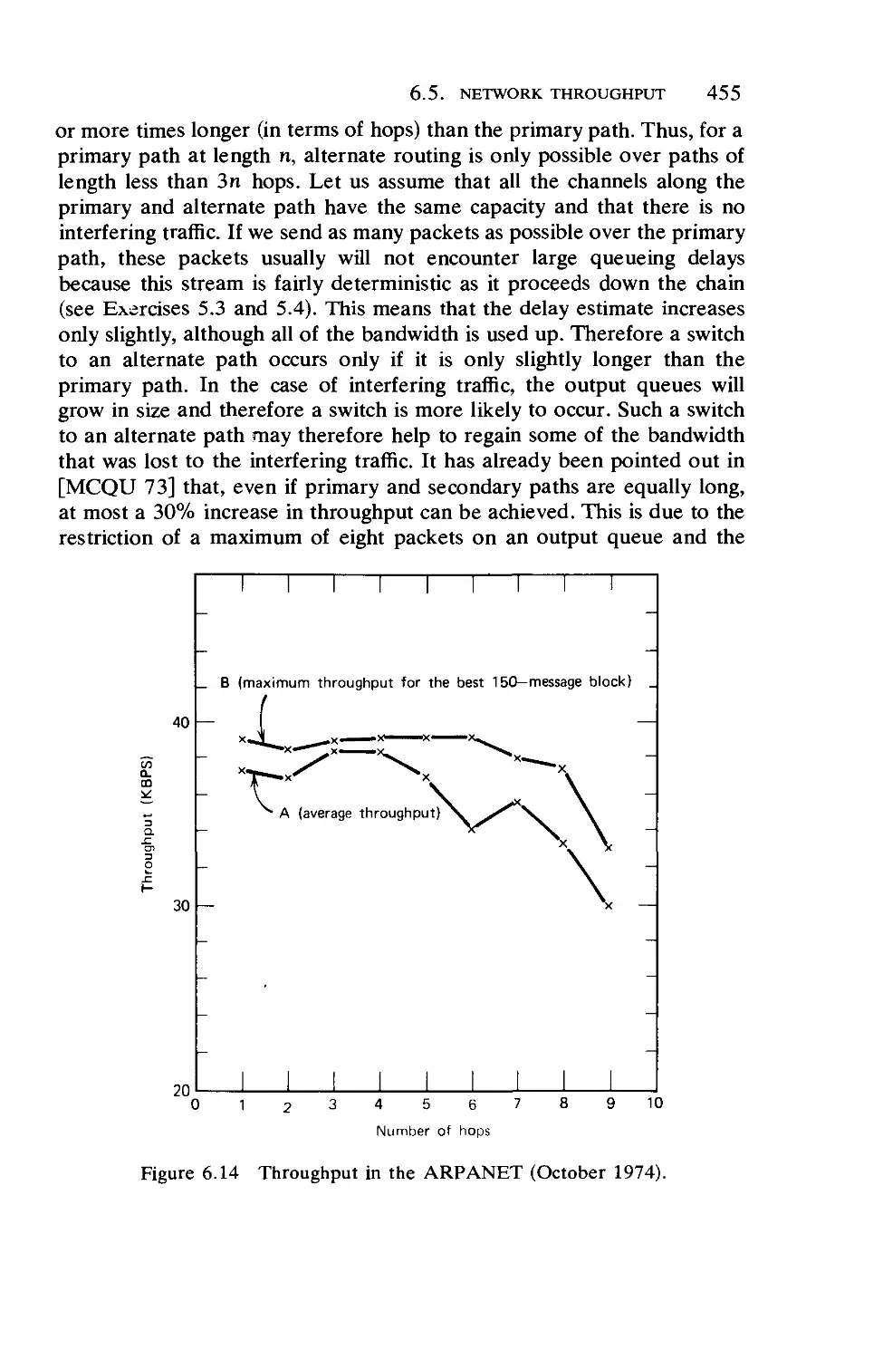
Network Throughput
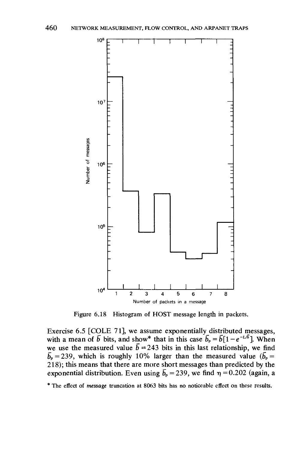
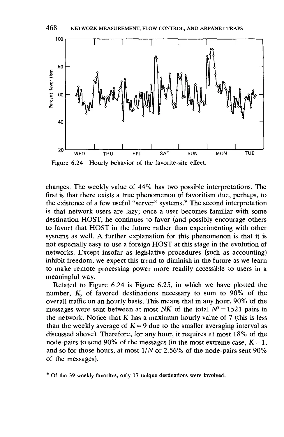
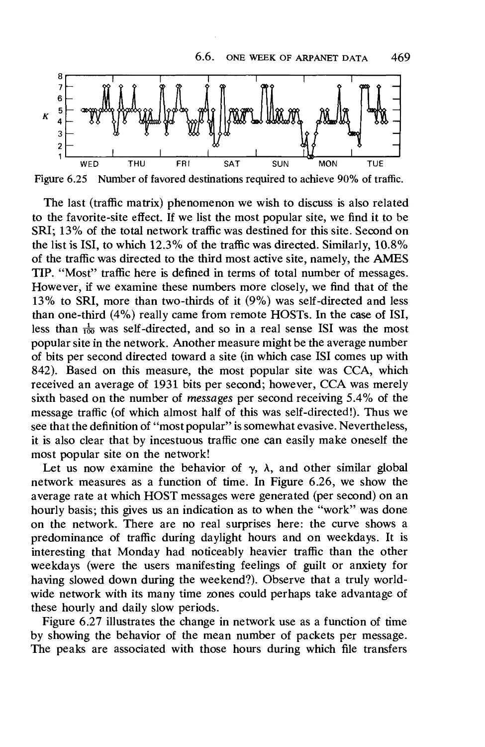
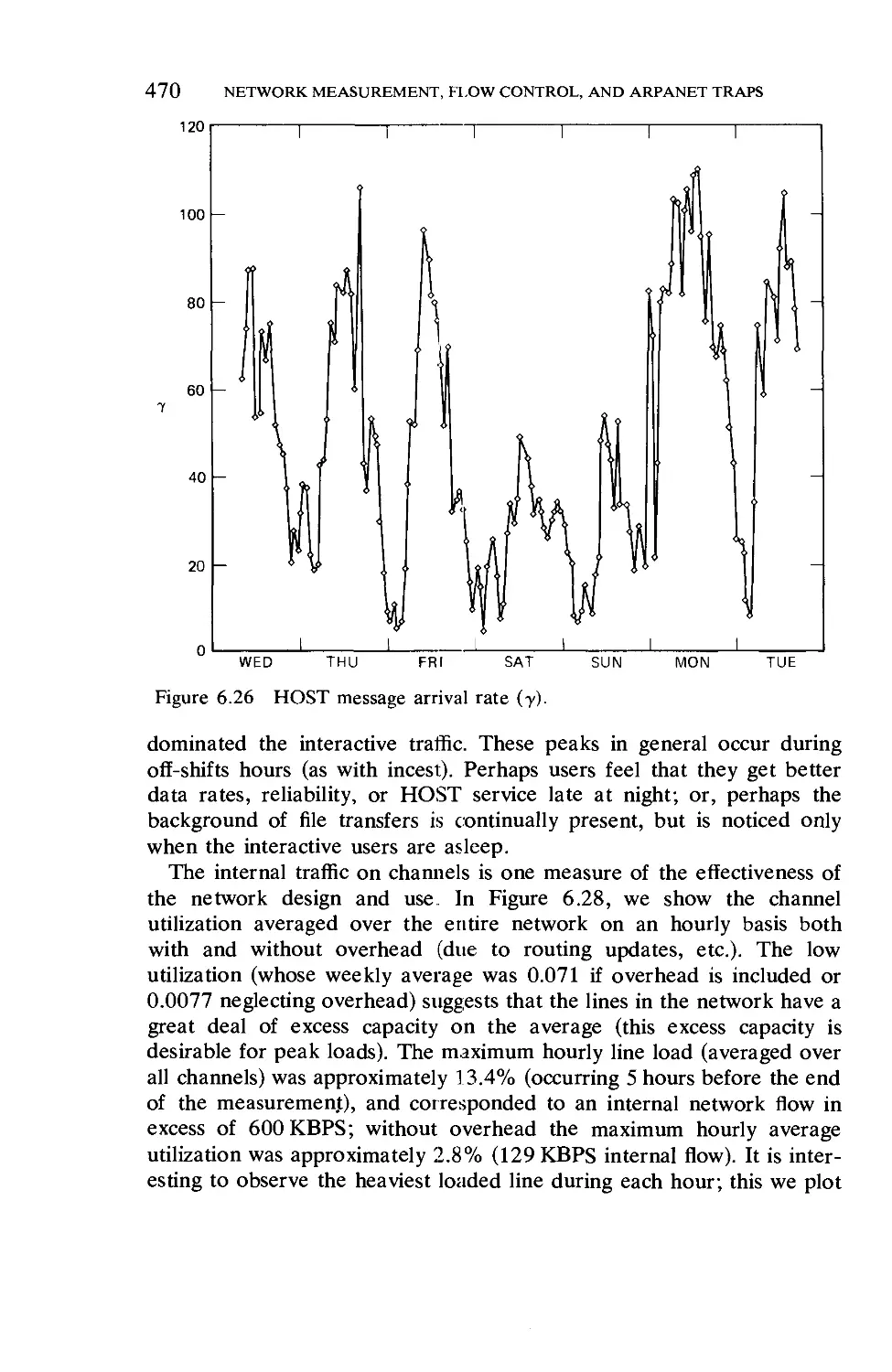
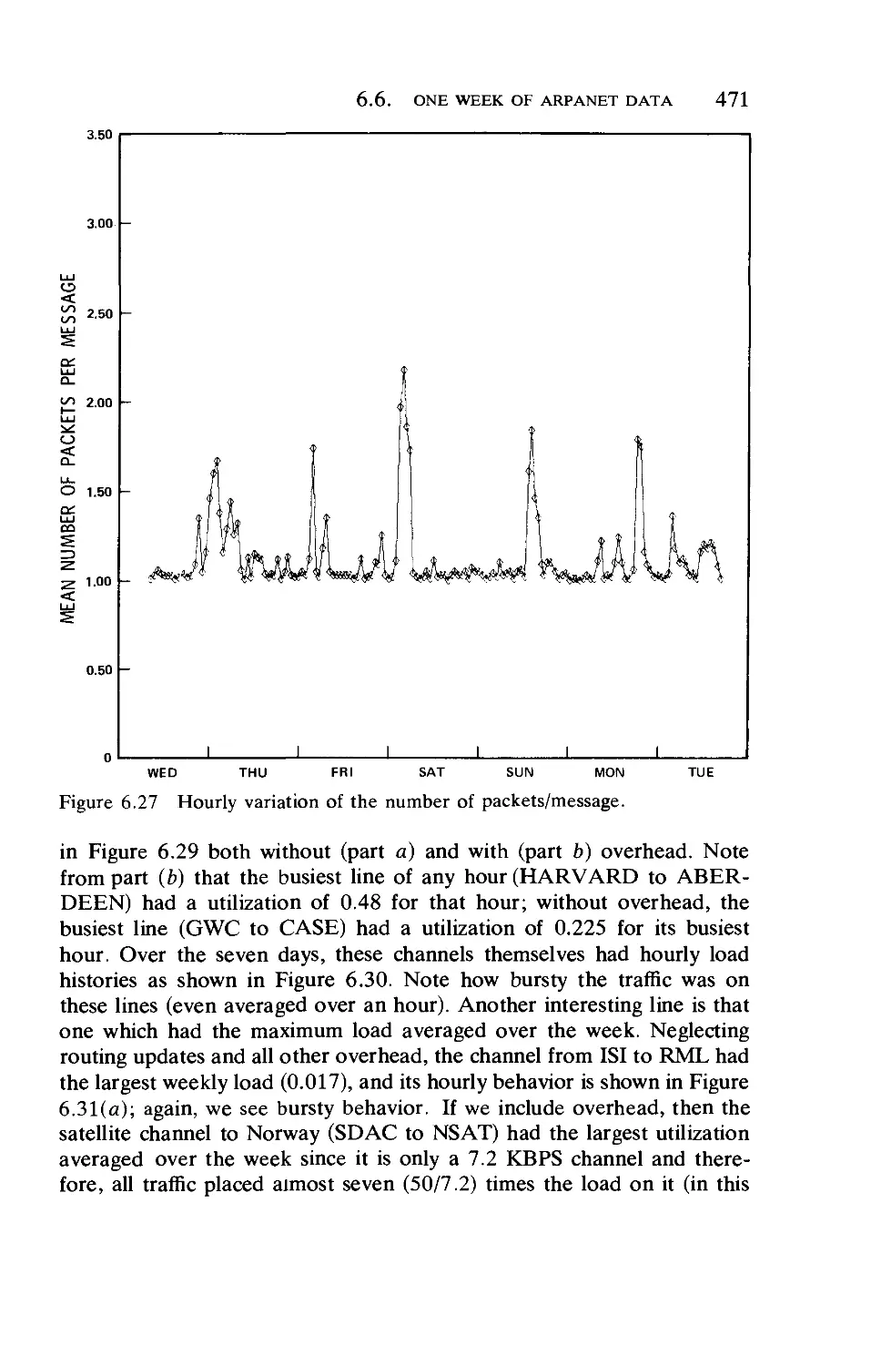
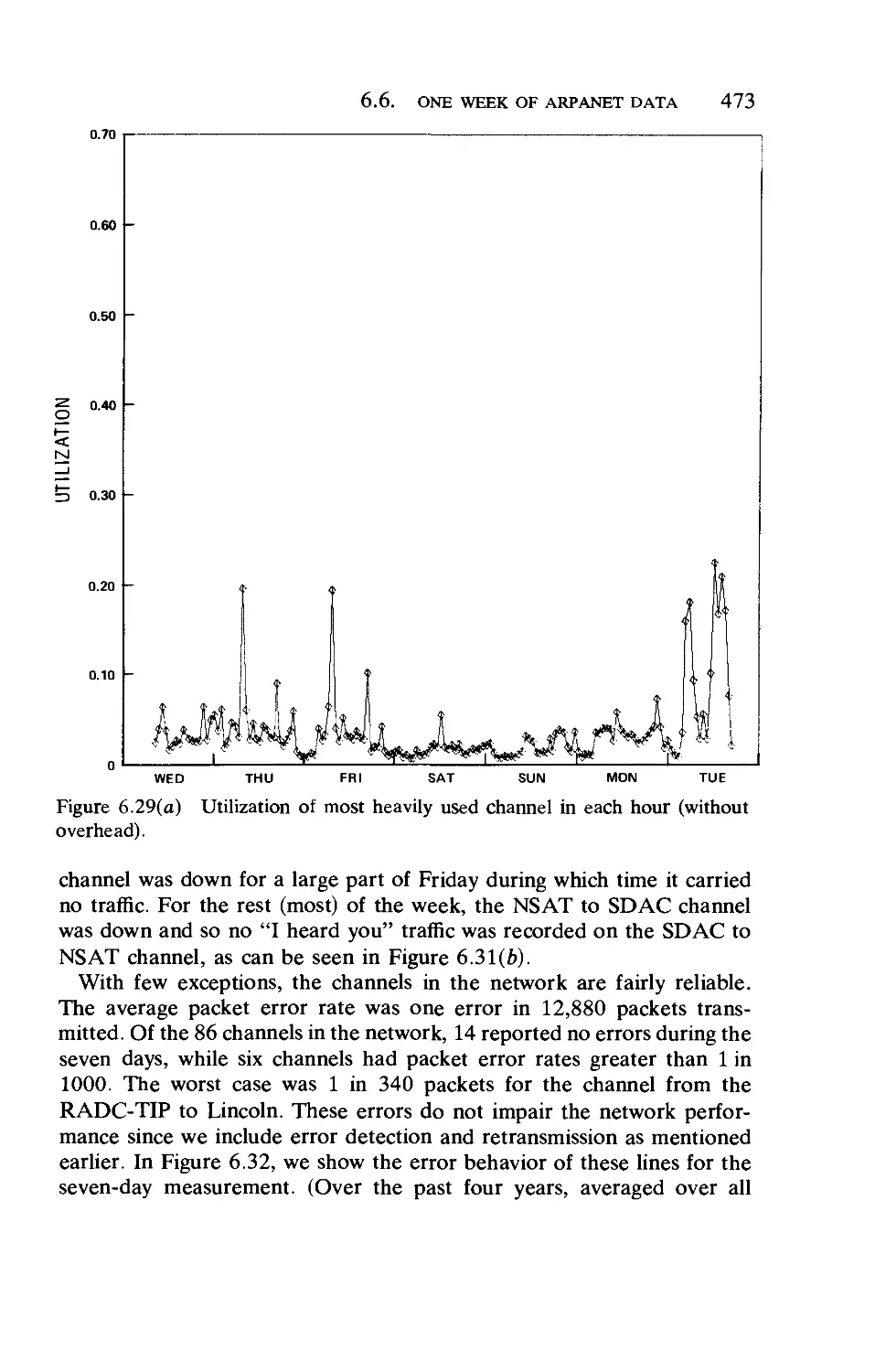
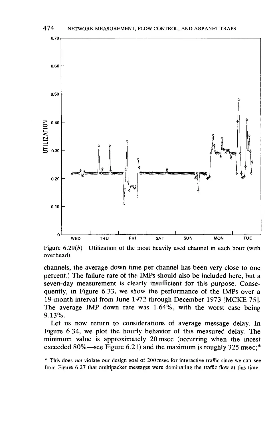
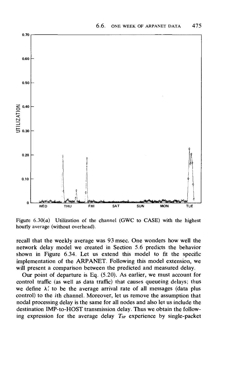
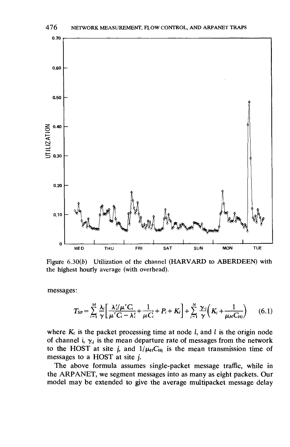
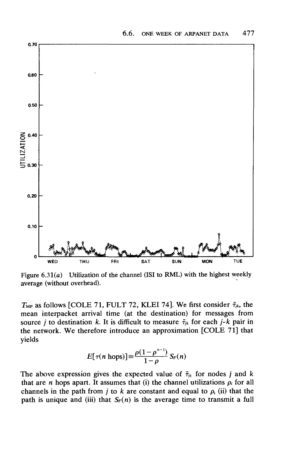
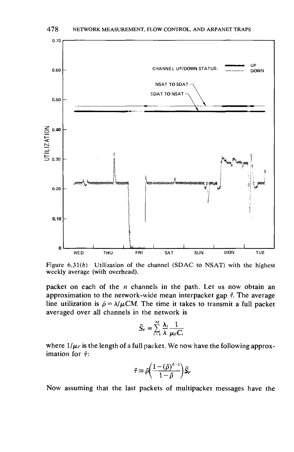
One Week of ARPANET Data
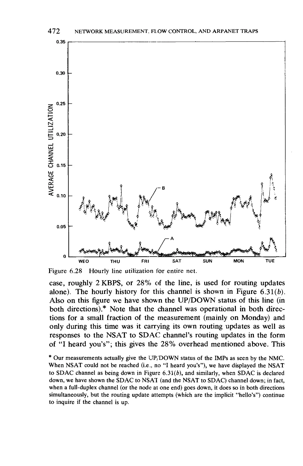
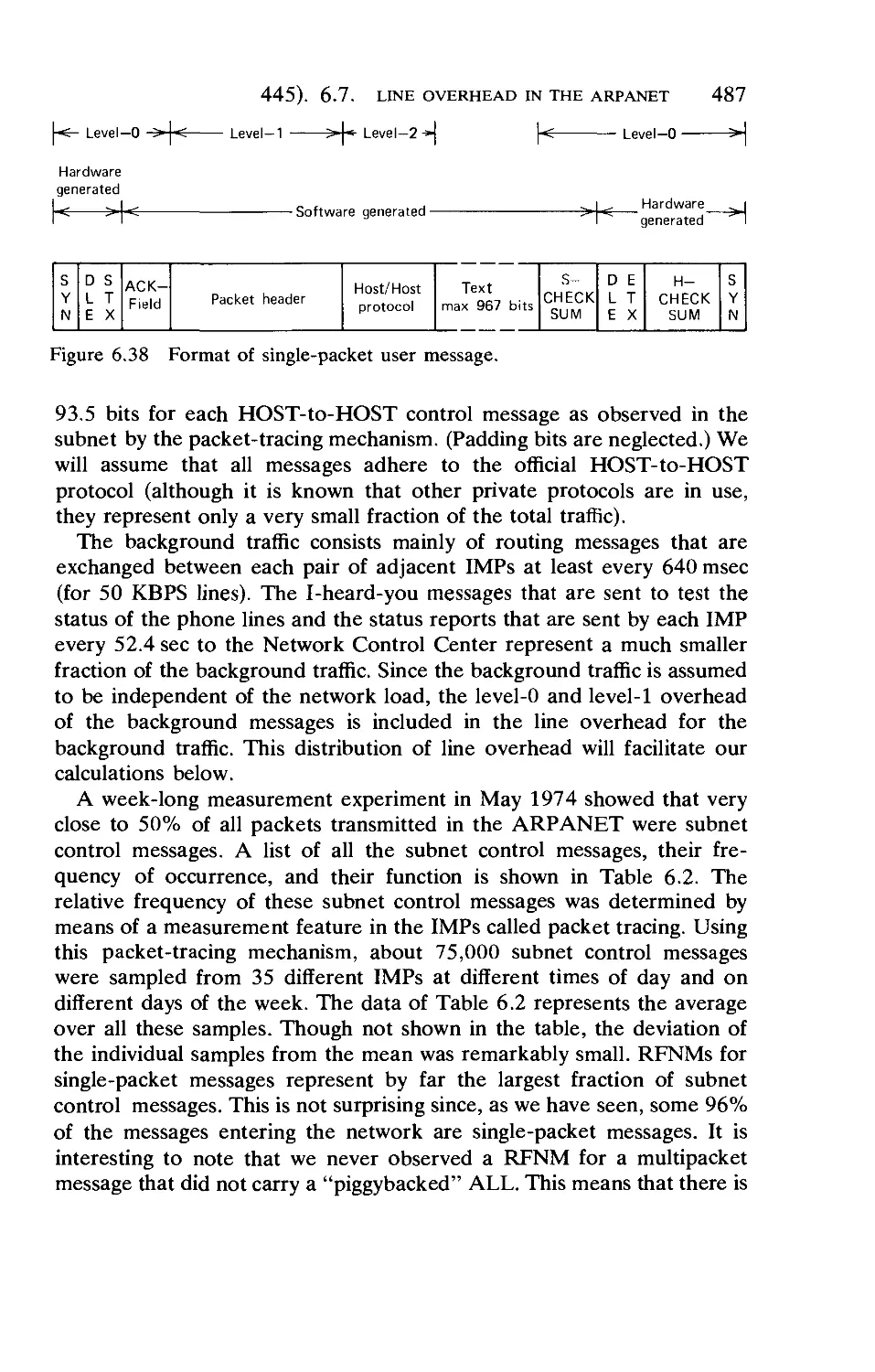
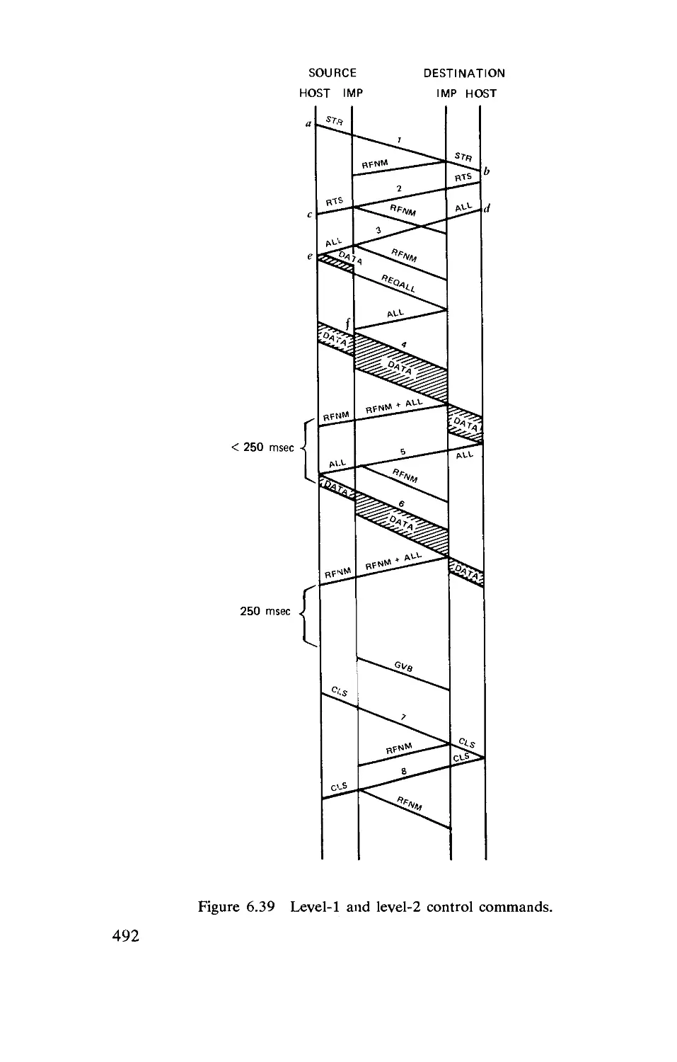
Line Overhead in the ARPANET . . . .
Recent Changes to the Flow Control Procedure
The Challenge of the Future
Summary c
»/ Important Results
422
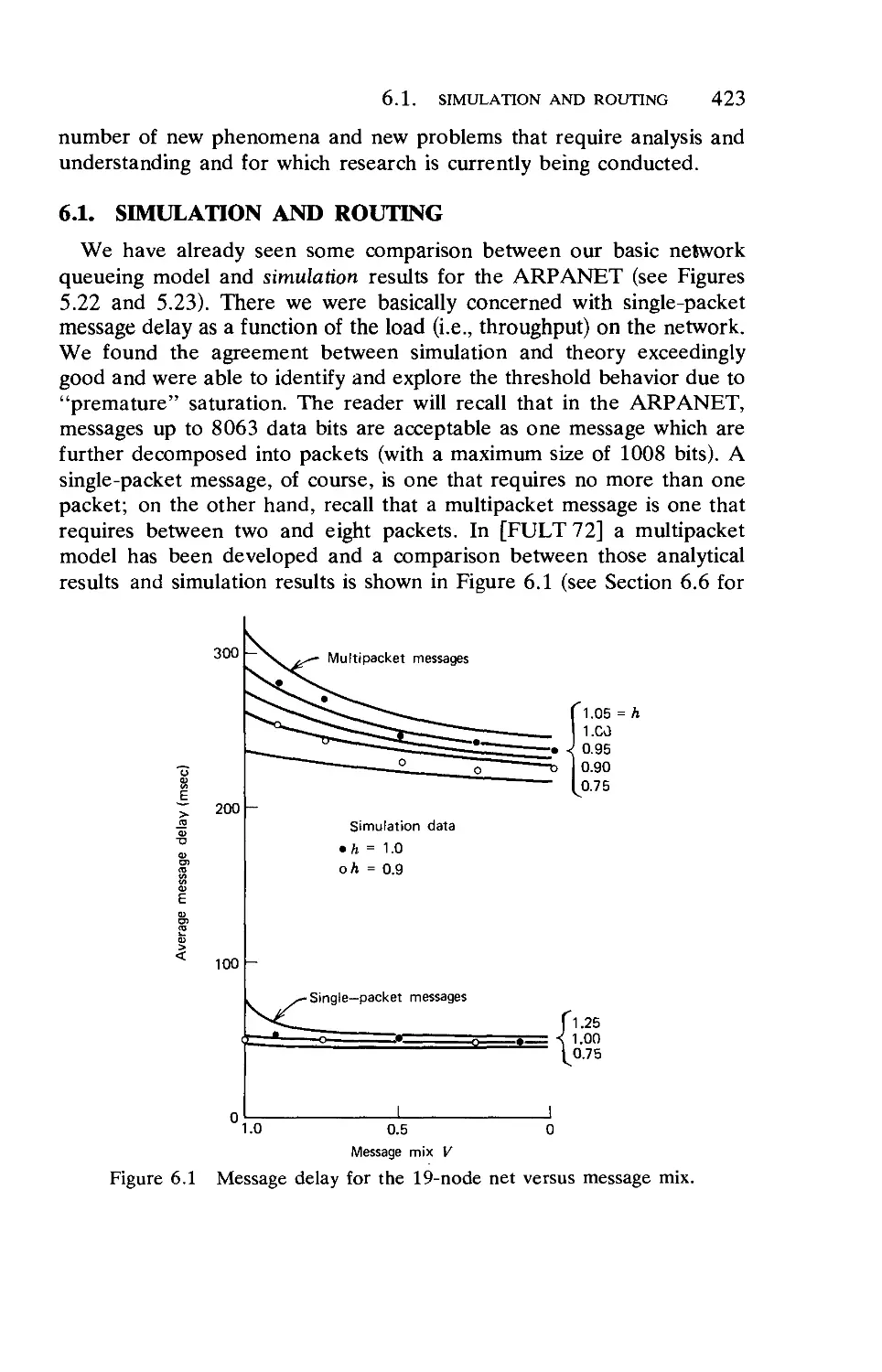
423
429
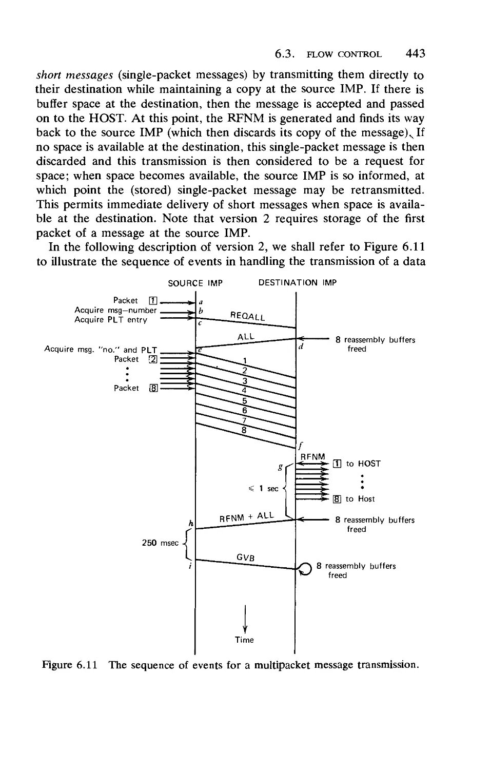
438
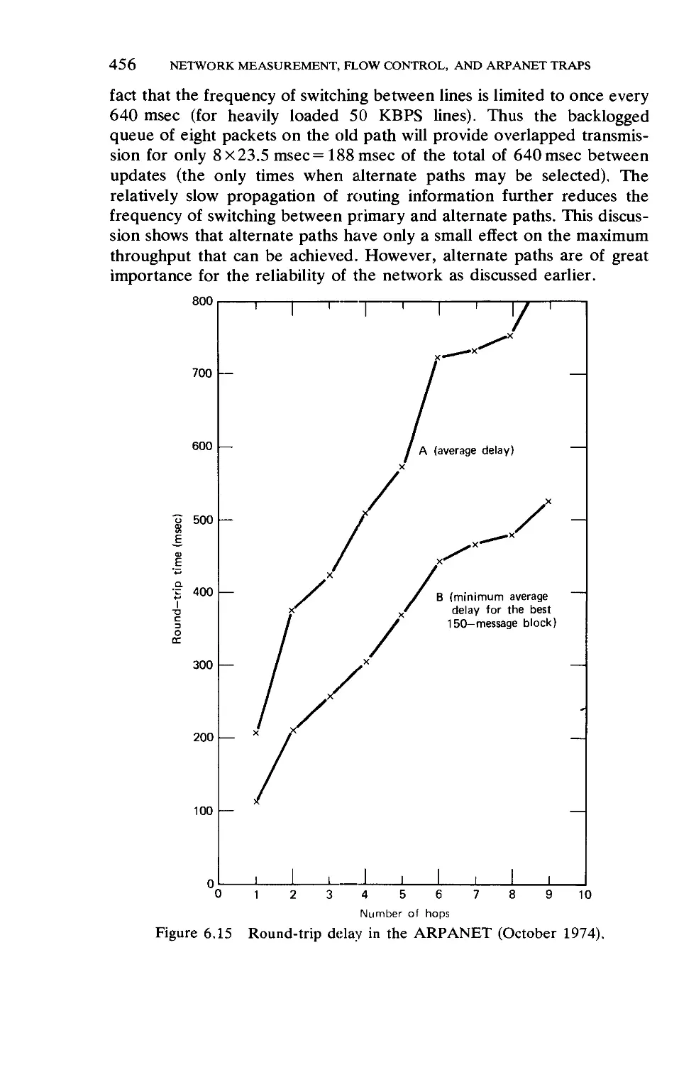
446
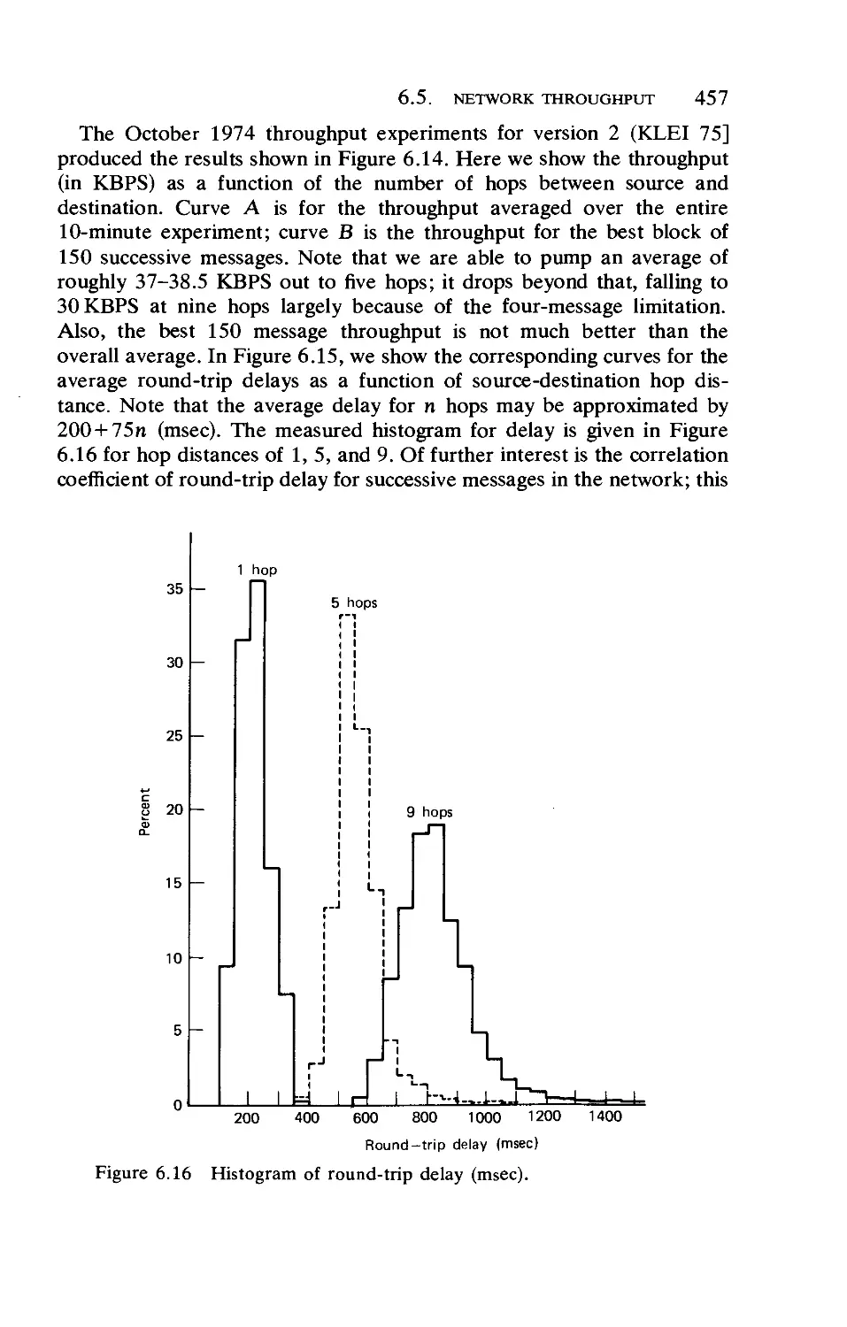
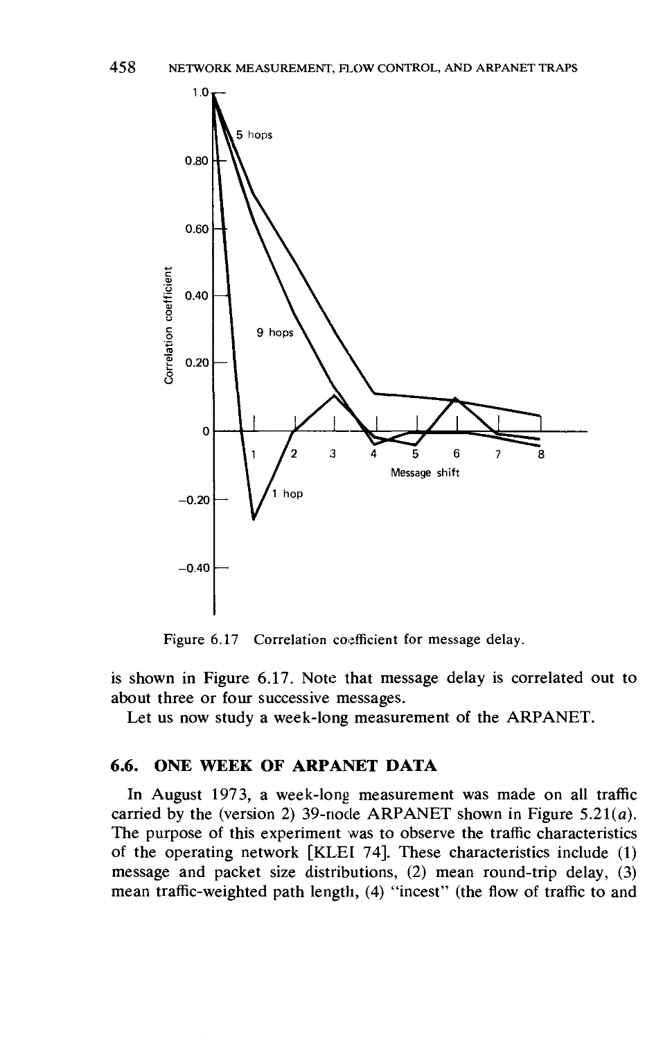
451
458
484
501
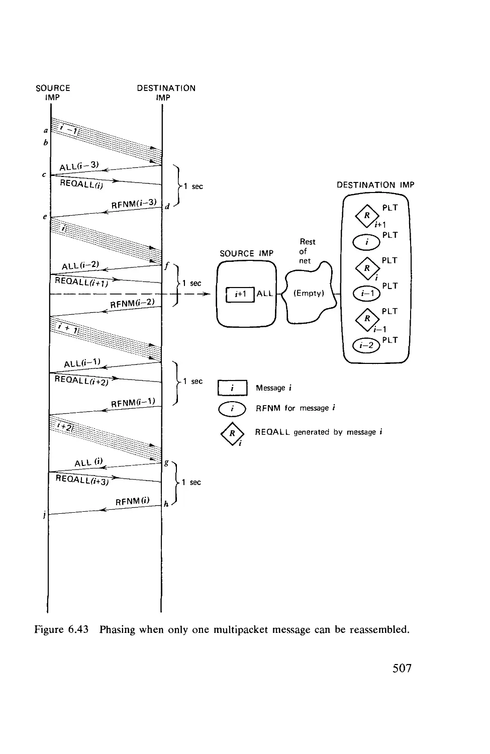
508
516
523
537
VOLUME I
part I: PRELIMINARIES
Chapter 1 Queueing Systems 3
1.1. Systems of Flow 3
1.2. The Specification and Measure of Queueing Systems 8
Chapter 2 Some Important Random Processes 10
2.1. Notation and Structure for Basic Queueing Systems 10
2.2. Definition and Classification of Stochastic Processes . 19
2.3. Discrete-Time Markov Chains 26
2.4. Continuous-Time Markov Chains .... 44
2.5. Birth-Death Processes 53
part II: ELEMENTARY QUEUEING THEORY
Chapter 3 Birth-Death Queueing Systems in Equilibrium
3.1. General Equilibrium Solution . . . .
3.2. M/M/l: The Classical Queueing System .
89
90
94
XV111 CONTENTS
3.3. Discouraged Arrivals 99
3.4. M/M/oo: Responsive Servers (Infinite Number of
Servers) 101
3.5. M/M/m: The m-Server Case 102
3.6. M/M/l/K: Finite Storage 103
3.7. M/M/m/m: m-Server Loss Systems 105
3.8. M/M/1//M: Finite Customer Population—Single
Server 106
3.9. M/M/00//M: Finite Customer Population—"Infinite"
Number of Servers 107
3.10. M/M/m/K/M: Finite Population, m-Server Case, Finite
Storage • 108
Chapter 4 Markovian Queues in Equilibrium 115
4.1. The Equilibrium Equations 115
4.2. The Method of Stages—Erlangian Distribution Er . 119
4.3. The Queue M/E,/l 126
4.4. The Queue E^M/1 130
4.5. Bulk Arrival Systems 134
4.6. Bulk Service Systems 137
4.7. Series-Parallel Stages: Generalizations .... 139
4.8. Networks of Markovian Queues 147
part III: INTERMEDIATE QUEUEING THEORY
Chapter 5 The Queue M/G/l 167
5.1. The M/G/l System 168
5.2. The Paradox of Residual Life: A Bit of Renewal
Theory 169
5.3. The Imbedded Markov Chain 174
5.4. The Transition Probabilities 177
5.5. The Mean Queue Length 180
5.6. Distribution of Number in System . . . .191
5.7. Distribution of Waiting Time 196
5.8. The Busy Period and Its Duration .... 206
5.9. The Number Served in a Busy Period . . . .216
5.10. From Busy Periods to Waiting Times . . . .219
5.11. Combinatorial Methods 223
5.12. The Takacs Integrodiflerential Equation . . . 226
CONTENTS XIX
Chapter 6 The Queue G/M/m 241
6.1. Transition Probabilities for the Imbedded Markov
Chain (G/M/m) 241
6.2. Conditional Distribution of Queue Size . . . 246
6.3. Conditional Distribution of Waiting Time . . . 250
6.4. The Queue G/M/l 251
6.5. The Queue G/M/m 253
6.6. The Queue G/M/2 256
Chapter 7 The Method of Collective Marks 261
7.1. The Marking of Customers 261
7.2. The Catastrophe Process 267
part IV: ADVANCED MATERIAL
Chapter 8 The Queue G/G/l 275
8.1. Lindley's Integral Equation 275
8.2. Spectral Solution to Lindley's Integral Equation . . 283
8.3. Kingman's Algebra for Queues 299
8.4. The Idle Time and Duality 304
Epilogue 319
Appendix I: Transform Theory Refresher: z-Transform and
Laplace Transform
1.1. Why Transforms? 321
1.2. The z-Transform 327
1.3. The Laplace Transform 338
1.4. Use of Transforms in the Solution of Difference and
Differential Equations 355
Appendix II: Probability Theory Refresher
II. 1. Rules of the Game 363
11.2. Random Variables 368
11.3. Expectation 377
11.4. Transforms, Generating Functions, and Characteristic
Functions 381
11.5. Inequalities and Limit Theorems 388
11.6. Stochastic Processes 393
XX CONTENTS
Glossary of Notation 396
Summary of Important Results 400
Index
411
QUEUEING SYSTEMS
VOLUME II: COMPUTER APPLICATIONS
I
A Queueing Theory Primer
In this chapter we summarize the important results to which one is
exposed in a first course on queueing theory. This material is drawn from
the companion volume [KLEI75] in which will be found a list of results
that key the reader to the location where each result is derived. Our
purpose is to lay the foundation for the remainder of the book, which is
devoted to the application of this theory in real-world situations; these
applications require sound judgment and experience in formulating
models as well as in developing operational formulas (exact or approximate)
that may be used for analysis and design of systems. We give a rather
complete review here (by stating—not deriving—results) so that this
material will form a self-contained body of results, to be used in later
chapters.
Consider any system that has a capacity C, the maximum rate at which
it can perform work. Assume that R represents the average rate at which
work is demanded from this system. One fundamental law of nature
states that if R < C then the system can "handle" the demands placed
upon it, whereas if R > C then the system capacity is insufficient and all
the unpleasant and catastrophic effects of saturation will be experienced.
However, even when J?<C we still experience a different set of
unpleasantnesses that come about because of the irregularity of the
demands. For example, consider the corner telephone booth, which on the
average can handle the load demanded of it. Suppose now that two people
approach that telephone booth almost simultaneously; it is clear that only
one of the two can obtain service at a given time and the other must wait
in a queue until that one is finished. Such queues arise from two sources:
the first is the unscheduled arrival times of the customers; the second is
the random demand (duration of service) that each customer requires of
the system. The characterization of these two unpredictable quantities
(the arrival times and the service times) and the evaluation of their effect
on queueing phenomena form the essence of queueing theory. In the
following section we introduce some of the usual notation for queueing
systems and then we proceed to summarize the major results for various
systems.
1
2 A QUEUEING THEORY PRIMER
1.1. NOTATION
Here we introduce only that notation required for the statement of
results in this chapter. A more complete listing is given in the glossary at
the end of the book.
We let C„ denote the nth customer to arrive at a queueing facility. The
important random variables to associate with C„ are
t„ = arrival time for C (1.1)
t„ = t„ - t„-i = interarrival time between C„ and C-i (1.2)
x„ = service time for C (1.3)
It is the sequence of random variables {t„} and {x„} that really "drives"
the queueing system. All these random variables are selected
independently of each other, and so we define the two generic random
variables
I = interarrival time (1.4)
x = service time (1.5)
Associated with each is a probability distribution function (PDF), that is,
A(t) = P[Tst] (1.6)
B(x) = P[x<x] (1.7)
and the related probability density function (pdf), namely,
a(f)=^5T (L8)
b(x)=^fr (1-9)
In this last definition for the pdf we permit the use of impulse functions as
discussed, for example, in Volume I of this text. The moments associated
with these random variables are denoted by
£[?]=?=} (1.10)
E[(l)k] = ? (1.11)
E[x] = x=- (1.12)
E[(x)k] = ? (1.13)
where the symbol (j, is often reserved only for the case of exponentially
distributed service times. Furthermore, we need the Laplace transform
1.1. NOTATION 3
associated with these pdf's, namely
E[e"sf] = A*(s) (1.14)
E[e sx~] = B*(s) (1.15)
The integral representation of this transform [say for a(t)] is simply
A*(s)=[ a(t)e-s,dt (1.16)
A key use of this transform is its moment generating property; for
example, the moments tk may be generated from A*(s) through the
relationship
dkA*(s)
ds
= (-l)V (1.17)
s=0
We often denote the kth derivative of a function f(t) evaluated at t = to by
= f(k)(to) (1.18)
dkf(t)
dtk
Thus Eq. (1.17) may be written as A*ik\0) = (-l)ktk.
Both I and x are the input random variables to the queueing system;
now we must define some of the important performance variables, namely,
the number of customers in the system, the waiting time per customer,
and the total time that a customer spends in the system, that is,
N(t) = number of customers in system at time t (1.19)
w„ = waiting time (in queue) for C (1.20)
s„ = system time (queue plus service) for G. (1.21)
The corresponding limiting random variables (after the system has been
in operation a long time) for a stable queue are N, vv, and s. As with I and
x we may define the PDF, the pdf, the first moment, and the appropriate
transform for N, vv, and s as follows:
P[N<k] W(y) = P[w<y] S(y) = P[s<y]
P[N=k] w(y) = ^ s(y) = ^l
E[N] = N E[w]=W E[s]=T
E[zN] = Q(z) E[e-s*]=W*(s) E[e"sS]= S*(s)
4 A QUEUEING THEORY PRIMER
The study of queues naturally breaks into three cases: elementary
queueing theory, intermediate queueing theory, and advanced queueing
theory. What distinguishes these three cases are the assumptions
regarding a(t) and b(x). In order to name the different kinds of systems we wish
to discuss, a rather simple shorthand notation is used for describing
queues. This involves a three-component description, A/B/m, which
denotes an m-server queueing system where A and B "describe" the
interarrival time distribution and service time distribution, respectively. A
and B take on values from the following set of symbols, which are meant
to remind the reader which distributions they refer to:
M = exponential (i.e., Markovian)
Er = r-stage Erlangian
HR = R-stage Hyperexponential
D = Deterministic
G = General
Specifically, if one of these symbols were used in place of B then it would
refer to the following pdf (x > 0):
M: b(x) = (j,e^x (1.22)
Er: b(,) = at(pCp: (1.23)
HR: b(x) = t <W<" (to, = l) (naO) (1-24)
i=l \i-l /
D: b(x) = u„(x --) (1.25)
G: b(x) is arbitrary
where in the next to last expression u0(x - 1/fi) refers to a unit impulse
occurring at the position x = 1/fA. Any distribution is permitted when G is
assumed. Pccasionally we add one or two more items to our three-
component description in order to describe the system's storage capacity
(denoted by K) or the size of the customer population (denoted by M), and
these will be commented on appropriately when used (otherwise they are
assumed to be infinite). The simplest interesting system we consider in this
chapter is the M/M/l queue in which we have exponential interarrival
times, exponential service times, and a single server (see Section 1.4). The
most complicated system we consider in this chapter is G/G/l in which the
exponential distributions are replaced by arbitrary distributions (see
Sections 1.2 and 1.10). In this review the majority of our results apply only
1.2. GENERAL RESULTS 5
to the first-come-first-serve queueing discipline; in Chapter 3, we study
the effect of other queueing disciplines. Let us now proceed with our
summary of results.
1.2. GENERAL RESULTS
Perhaps the most important system parameter for G/G/l is the
utilization factor p, denned as the product of the average arrival rate of
customers to the system times the average service time each requires, that
is,
p=Ax (1.26)
This quantity gives the fraction of time that the single server is busy and is
also equal to the ratio of the rate at which work arrives to the system
divided by the capacity of the system to do work, that is, R/C as discussed
earlier.* In the multiple-server system G/G/m the corresponding
definition is
which also is equal to R/C and may be interpreted as the expected
fraction of busy servers when each server has the same distribution of
service time; more generally, p is the expected fraction of the system's
capacity that is in use. In all cases a stable system (one that yields finite
average delays and queue lengths) is one for which
0<p<l (1.28)
and we note that the case p = 1 is not permitted (except in the very
special situation of a D/D/m queue). As we shall see, the closer p
approaches unity, the larger are the queues and the waiting times; it is
this quantity that essentially reflects the way in which the system
performance varies with the average system load.
The average time in system is simply related to the average service time
and the average waiting time through the fundamental equation
T = x + W (1.29)
and it is the quantity W that reflects the price we must pay for sharing a
given resource (server) with other customers. Whereas p is the most
important system parameter, it is fair to say that one of the more famous
* On the average, A customers arrive per second and each brings x sec of work for the
system; thus R = Ax. The (single-server) system can perform 1 sec of work per second of
elapsed time, and so C= 1.
6 A QUEUEING THEORY PRIMER
formulas from queueing is Little's result, which relates the average
number in the system to the average arrival rate and the average time
spent in that system, namely,
N = \T (1.30)
This result enters most of the calculations we make in this book and is
extremely general in its application. The corresponding result for number
and time in queue is simply given by
Nq=\W (1.31)
where Nq is merely the average queue size. Furthermore, it is true in
G/G/m that these quantities are related by*
Nq=N-mp (1.32)
We have already given one fundamental law that applies to queueing
systems, namely that R < C in order for the system to be stable. A second
common and general law of nature also finds its way into our analyses; it
relates the rate at which accumulation within a system occurs as a
function of the input and output rates to and from that system. In
particular, if we let Ek denote the system state in which k customers are
present and if we let
P*(t) = P[N(t) = k] (1.33)
which is merely the probability that the system state at time t is Ek, then,
loosely stated, we have
—-^-^ = [flow rate of probability into Ek at time t]
-[flow rate of probability out of Ek at time t] (1.34)
Equation (1.34) will allow us to write down time-dependent relationships
among the system probabilities in a straightforward fashion. Now
consider a stable system, for which the probability Pk(t) has a limiting value
(as t —>o°) which we denote by pk, (this represents the fraction of time
that the system will contain k customers in the steady state). If the
interarrival times are exponentially distributed (that is, they form a
Poisson arrival process), then the equilibrium probability, rk, that an
arriving customer finds k in the system upon his arrival will in fact equal
the long-run probability of there being k customers in the system, that is
pk = rk. On the other hand, if we denote by dk the equilibrium probability
that a departure leaves behind k customers in the system, then dk = rk if
*This follows from T = x + W and Little's result.
1.3. MARKOV, BIRTH-DEATH, AND POISSON PROCESSES 7
the system state N(t) is permitted to change by at most one at any time.
Thus, if we have unit state changes and Poisson arrivals, then we have the
situation in which pk = rk = dk.
1.3. MARKOV, BIRTH-DEATH, AND
POISSON PROCESSES
Before we proceed to discuss the results for elementary queueing
systems it is convenient to list some of the well-known results for some
simple and important random processes that form the foundation for the
queueing results we shall quote.
We begin with discrete-state discrete-time Markov processes such that
X„ denotes the discrete value of the (random) process at its nth step. The
defining condition for such a Markov chain is
P[Xn = /1 X.-i = L-u..., Xx = ii] = P[Xn = /1 X.-i = in-x] (1.35)
This is merely an expression of the fact that the present state completely
summarizes all of the pertinent past history so far as that history affects
the future of the process. If we let
Tri<n) = P[X„ = i] (1.36)
and denote the vector of these probabilities by
^"^[irf'.ir?0,...] (1.37)
and moreover if we denote the one-step transition probabilities for
homogeneous Markov chains by
pi,=P[Xn=/|Xn-1 = i] (1.38)
and collect these into a square matrix denoted by P = (pi,), then we have
the basic results for the time-dependent probabilities of this Markov
process, namely,
w<n)=1I(n-l)p (139)
w<n) = 1I(0)p„ (14Q)
The sequence Pn (n =0,1,2,...) is equal to the inverse z-transform of
the matrix [I-zP]"1, where I represents the identity matrix and -1 refers
to the matrix inverse. The more useful steady-state behavior of these
probabilities may be found by solving the equation
7T = 7TP
(1.41)
8 A QUEUEING THEORY PRIMER
along with the condition that
Z it, = 1 (1.42)
i-0
where we have used the notation tti = lim„^ tt^\ Finally, we comment
that the time the process spends in any state is geometrically distributed
(an inherent property of all Markov processes); this distribution is, of
course the only discrete memoryless distribution.
Let us now consider the case of a discrete-state continuous-time
homogeneous Markov process X(t); here we have a denning property
much as we did in Eq. (1.35). The time the process spends in any state is
exponentially distributed for all continuous-time Markov processes; this is
the only (continuous) memoryless distribution, and it is this property that
makes the analysis simple. We now define the transition probabilities as
Pi,(0 = P[X(s + t) = j\ X(s) = i] (1.43)
The matrix of these transition probabilities will be denoted by H(t), and
in terms of this matrix we may express the Chapman-Kolmogorov
equations as
H(«)=--H(t-s)H(s) (1-44)
In a real sense H(t) corresponds to P" and that which corresponds to P
itself is H(At) (namely the transition probabilities over an infinitesimal
interval). Of more use is the matrix Q = [q.J, referred to as the
infinitesimal generator of the process; it is defined by
Q=limH(A0zI (145)
^ A.-.0 At
In terms of this matrix we may then express the time-dependent behavior
of our Markov process by the equation
dH(f)=H(t) (146)
at
whose solution is
H(t) = eQ' (1.47)
The steady-state behavior of this process, namely, the stable probabilities
it, are given through the basic equation
nQ = 0 (1.48)
along with the normalizing equation (1.42). We have occasion to discuss
the discrete-state continuous-time and continuous-state continuous-time
1.3. MARKOV, BIRTH-DEATH, AND POISSON PROCESSES 9
processes in Chapter 2 below. (A more complete summary for Markov
chains is given in tabular form in the summary of results in Volume I.)
Perhaps the most fundamental random process we encountei in queue-
ing theory is the Poisson process that describes a collection of arrivals for
which the interarrival times are independent and exponentially
distributed with a mean interarrival time F = 1/A. In particular, the probability
Pk(t) of k arrivals in an interval whose duration is t sec is given by
Pk(t) = (~fe-K' (1.49)
The average number of arrivals during this interval is merely
N(t)=kt (1.50)
and the variance is given by
alm = \t (1.51)
We note that the mean and variance for this process are identical. The
z-transform for this process is simply given by
E[zN(,)] = cWl-" (1.52)
The assumption of an exponential interarrival time means, of course,
a(t) = ke-" t>0 (1.53)
which, we repeat, is the memoryless distribution. Here, the mean and
variance are, respectively, I = 1/A and a2= 1/A2.
Among the class of continuous-time Markov processes there is the
special case of birth-death processes in which the system state changes by
at most one (up or down) in any infinitesimal interval. In such cases we
talk about the birth rate Ak, which is the average rate of births when the
system contains k customers, and also of the death rate fj*, which is the
average rate at which deaths occur when the population is of size k. The
time-dependent behavior for such a system is essentially given in Eq.
(1.47). The equilibrium behavior as defined in Eq. (1.48) takes on an
especially simple form for this class of birth-death processes whose
solution is given as follows (here we use the more usual notation pk rather
than 7Tic to denote the probability of having k customers in the system):
Pk=Pofi-^- (1.54)
i=0 fAi + i
with the constant p0 being evaluated through
po = ra (1.55)
10 A QUEUEING THEORY PRIMER
The application of this equilibrium solution leads us directly to the class
of elementary queueing systems which we discuss in the next three
sections.
1.4. THE M/M/l QUEUE
The M/M/l queue is the simplest interesting queueing system we
present. It is the classic example and the analytical techniques required
are rather elementary. Whereas these techniques do not carry over into
more complex queueing systems, the behavior of M/M/l is in many ways
similar to that observed in the more complex cases.
Since this system has a Poisson input (with an average arrival rate A)
and makes unit step changes (single service and single arrivals), then
Pic = rk = die. (Recall that the average service time is x = 1/p,.) This
distribution is given by
p.-d-pK (1-56)
and so we immediately find that the average number in the system is
given by
N = ^ (1.57)
with variance
<tn = d_0y (1.58)
Using Little's result and Eq. (1.32), we may immediately write down the
two basic performance expressions for average delays in M/M/l:
W = f^ (1.59)
T = ^ (1.60)
1-p
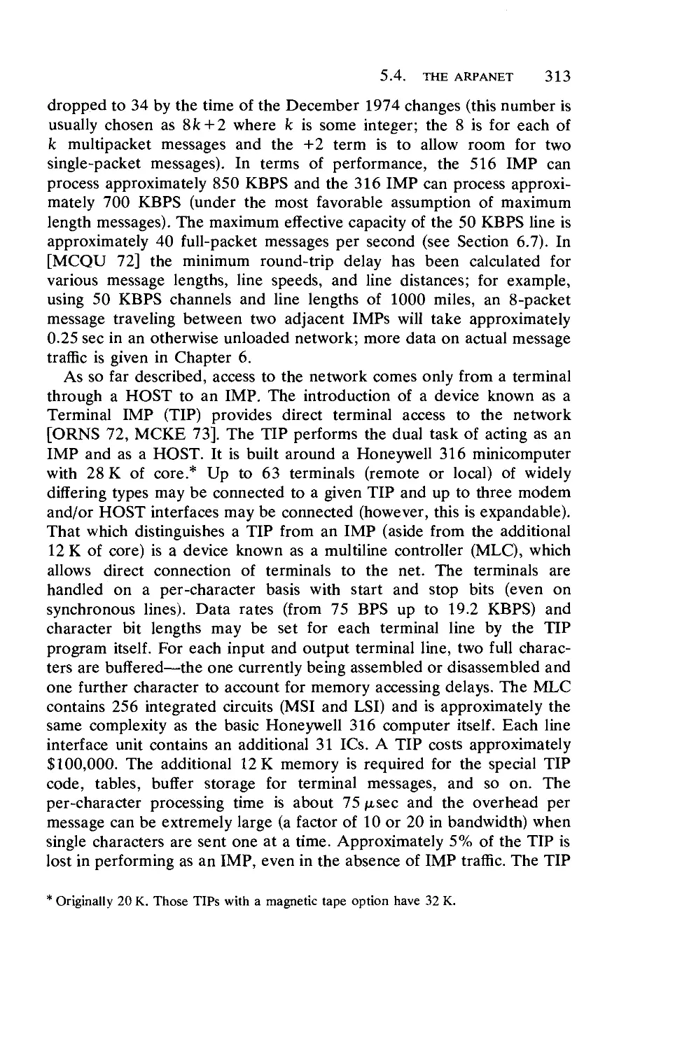
The terms N, W, and T all demonstrate the same common behavior as
regards the utilization factor p; namely, they all behave inversely with
respect to the quantity (1 - p). This effect is dominant for M/M/l as well
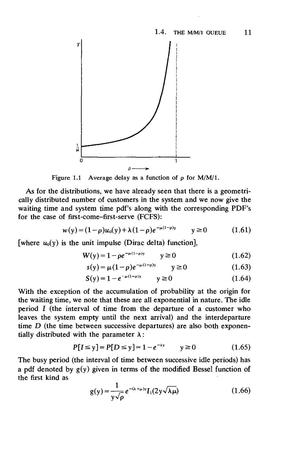
as for most common queueing systems, and in Figure 1.1 we show the
average time in system as a function of the utilization factor. Thus as p
approaches unity from below, these average delays and queue sizes grow
without bound! This is true of essentially every queueing system one will
encounter and shows the extreme price that must be paid if one is
interested in running the system close to its capacity (p = 1).
1.4. THE M/M/l QUEUE
11
Figure 1.1 Average delay as a function of p for M/M/l.
As for the distributions, we have already seen that there is a
geometrically distributed number of customers in the system and we now give the
waiting time and system time pdf's along with the corresponding PDF's
for the case of first-come-first-serve (FCFS):
w(y) = (l-p)uo(y) + A(l-p)e-'1<1-p)y y>0
[where u0(y) is the unit impulse (Dirac delta) function],
W(y) = l-pe_M1-ph y>0
s(y) = (j,(l-p)e
S(y) = l-e
-H.(l-p)y
y>0
-^(l-p)y
y>0
(1.61)
(1.62)
(1.63)
(1.64)
With the exception of the accumulation of probability at the origin for
the waiting time, we note that these are all exponential in nature. The idle
period I (the interval of time from the departure of a customer who
leaves the system empty until the next arrival) and the interdeparture
time D (the time between successive departures) are also both
exponentially distributed with the parameter A:
P[I<y] = P[D<y]=l-e_i> y>0 (1.65)
The busy period (the interval of time between successive idle periods) has
a pdf denoted by g(y) given in terms of the modified Bessel function of
the first kind as
g(y) = -i=e-tt+^I1(2yVA^) (1.66)
yVp
12 A QUEUEING THEORY PRIMER
The probability /„ that n customers are served during a busy period is
given by
/n=^:j)p"-1(l+p)1-2" (1-67)
Two simple extensions for the M/M/l svstem are easily described. First,
there is the case of bulk arrivals where with probability gk a group of k
customers arrives at each arrival instant from the Poisson process; we
then define the generating function for this distribution as usual by
G(z) = X£=o gkZk with which we may then give the generating function for
the number of customers in this bulk arrival M/M/l system,* namely,
Q(2)= na-pxi-*)
(j,(l-z)-Az[l-G(z)]
The second generalization is a bulk service system in which a free server
will take up to, but no more than, r customers and serve them collectively
(as if they were a single customer) with an exponentially distributed
service time. The probability of finding k customers in this system is given
by
Ifc = (l--)(-)" k = 0,l,2,... (1.69)
\ Zo/\/o/
where z0 is that unique root lying outside the unit disk, that is, |z0| > 1, for
the equation
rpz,+1-(l + rp)z' +1=0 (1.70)
and where, as usual, p = A/r/x.
A final generalization, which we will use in Chapter 4, involves the case
of an M/M/l system with a finite number of customers, namely M, that
behave in the following way. A customer is either in the system (waiting
for or being served) or outside the system and arriving; the interval from
the time he leaves the system until he returns once again is exponentially
distributed with mean 1/A. This case gives the following expression for the
probability for finding k customers in the system:
^M!/(M-k)!](A/^ (171)
f;[M!/(M-0!](A/n)'
i-l)
* That is, recall Q(z) = E[zN], not to be confused with the infinitesimal generator Q
defined in Eq. (1.45).
1.5. THE M/M/m QUEUEING SYSTEM 13
So much for the classic M/M/l system. In the next section, we retain
the Markovian assumptions but consider the case of multiple servers.
1.5. THE M/M/m QUEUEING SYSTEM
We now consider the generalization to the case of m servers. A single
queue forms in front of this collection of m servers and the customer at
the head of the queue will be handled by the first available server. As
usual, A is the arrival rate and l//x is the average service time, with
p = A/m/x. The equilibrium probability of finding k customers in the
system is given by
where
(mpf
(p)kmm
po , k>m
(1.72)
A. K. Erlang, the father of queueing theory, considered this system as
one model for the behavior of telephone systems early in this century
[BROC 48]. Identified with his name is the Erlang-C formula, which gives
the probability that an arriving customer must wait for a server; his
expression is given by pm from Eq. (1.72). Extensive tables of this
quantity are available in the many books dealing with telephony
[TELE 70].
Further results for M/M/m may be found in Section 1.9, which
discusses G/M/m. Specifically W and W(y) are given in Eqs. (1.113) and
(1.114), respectively, where for M/M/m we have simply that <r = p.
Erlang considered a second model for telephone systems that is the
same as M/M/m but permits no customers to wait; that is, it is a loss
system with at most m customers present at any one time. In this case,
the probability of finding k customers in the system is given by
^MnOhL (1.74)
I (WW
i=0
for the range 0 ^ k < m. The important quantity of interest here is the
probability that a customer upon arrival to the system will find no empty
servers and will therefore be "lost;" this is referred to as the Erlang-B
formula or as Erlang's Loss Formula (also commonly tabulated) and is
given simply by pm from Eq. (1.74).
14 A QUEUEING THEORY PRIMER
1.6. MARKOVIAN QUEUEING NETWORKS
Before leaving the comfortable world of exponential distributions, we
wish to discuss another class of results that applies to networks of queues
in which customers move from one queueing facility to another in some
random fashion until they depart from the system at various points.
Specifically, we consider an N-node network in which the ith node
consists of a single queue served by tru servers, each of which has an
exponentially distributed service t:ime of mean l//xi. The ith node receives
from outside the network a sequence of arrivals from an independent
Poisson source at an average rate of ji customers per second. When a
customer completes service at the ith node he will proceed next to the jth
node with probability ry; thus he becomes an "internal" arrival to the jth
node. On the other hand, upon leaving the ith node a customer will
depart from the entire network with probability 1 — Sii »«• We define the
total arrival rate to the ith node to be, on the average, \t customers per
second, and this consists both of external and internal arrivals. The set of
denning equations for \, is given by
N
Ai^Yi + IVii (1.75)
i-i
A large measure of independence exists among the nodes in such a
network, as may be seen from the expression given below for the joint
distribution of finding ki customers in the first node, k2 customers in the
second node, and so on:
p(ki, k2,..., kN) = pi(ki)p2(k2)... pN(kN) (1.76)
The factoring of this joint distribution exposes the independence. In
Chapters 4 and 5 we are delighted to take advantage of this
independence. In particular, each factor in this last expression, say p.(ki), is
merely the solution to an isolated M/M/nii queueing facility operating by
itself with an input rate A;; the solution for p.(ki) is given in Eq. (1.72).
Another class of Markovian queueing networks consists of those
networks in which customers are permitted neither to leave nor to enter. In
particular, we assume that K customers are placed (trapped) within a
network similar to the one described above and that they move around
from node to node, but no departures from any node are permitted; that
is, 1 — SfL i n, = 0 for all i. These closed networks have the following
solution for the joint distribution of finding customers in various nodes:
p{k-k----kN)=GmUm) (L77)
1.7. THE M/G/l QUEUE 15
where the set of numbers {x;} must satisfy the following linear equations
[similar to Eq. (1.75) with 7, =0]:
IMX,
* = £wto i = l,2,...,N (1-78)
;-i
and where
°<->»'Mim ,L79)
where k = (ki, k2,..., kN) and A is that set of vectors k for which
ki + k2 + - • ■+kN = K and where
&(*<) = < t , (1-80)
These open and closed networks will be developed further in Chapter
4.
1.7. THE M/G/l QUEUE
In this and the following two sections we study systems that fall in the
domain of intermediate queueing theory. This classification refers to
those systems in which we permit either (but not both) the interarrival
time or the service time to be nonexponentially distributed; the case when
both these random variables are nonexponential forms part of advanced
queueing theory which we discuss in Section 1.10. For the M/G/l system
we cannot give explicit distributions for the number in system or for the
time in system as we did for the M/M/l system [specifically, see Eqs.
(1.56) and (1.64) above]. Rather, we find expressions for the transforms
of these distributions.
The M/G/l system is characterized by a Poisson arrival process at a
mean rate of A arrivals per second and with an arbitrary or general
service time distribution of form_B(x) with a mean service time of x sec
and with kth moment equal to x\ Due to the Poisson arrival process and
due to the fact that the number in the system changes by at most one, we
again have p* = rk = ck.
The basic (difference) equation describing the relationship among
random variables for this first-come-first-serve M/G/l system is
fq„-l+tt.+i ifq„>0
q„+1 = f 4 (1.81)
[Vn+i if q„ = 0
where q„ is the number of customers left behind by the departure of
customer C, and vn is the number of customers who enter during his
16 A QUEUEING THEORY PRIMER
service time (x„). The sequence {q„} forms a (discrete-state continuous-
time) Markov chain. The entire transient and equilibrium behavior for the
system is contained in this equation, and from it we may derive most of
our results for M/G/l.
By far the most well-known result for the M/G/l system is the
Pollaczek-Khinchin (P-K) mean value formula, which gives the following
compact expression for the (equilibrium) average waiting time in the
queue:
W = (T^) d-82)
The numerator term, denoted by W0 = Ax2/2, is, in fact, equal to the
expected time that a newly arriving customer must spend in the queue
while that customer (if any) which he finds in service completes his
remaining required service time.* From this formula one may easily
calculate T using Eq. (129); combining that result with the results quoted
in Eqs. (1.31) and (1.32) we easily come up with the P-K mean-value
formula for number in system as
Sf = p+*^!ll (1.83)
1-p
* This quantity is related to the concept of residual life, which we will use in this book. To
elaborate, let us consider the sequence of instants located on the real-time axis such
that the set of distances between adjacent points is a set of independent, identically
distributed random variables whose density we shall denote by /(x) (that is, we
are dealing with a renewal process). Let rn, denote the nth moment of these interval
lengths. Let us now select a point along the time axis at random; the interval in which this
point falls will be referred to as the "sampled" interval. The length of the sampled interval is
known as the lifetime of the interval, the time from the start of the sampled interval to this
point is known as the age of the interval, and the distance from this selected point until the
end of the sampled interval is known as the residual life of the interval. We are concerned
with the statistics of the residual life. The pdf for residual life is given by f(x) =
[l-F(x)]/(mO and the Laplace transform of this density is given by F*(s) =
[1-F*(s)]/(smO; the notation here is that F(x) = JS/(y) dy and F*(s) is the Laplace
transform associated with the pdf fix). Perhaps the most significant statistic is the mean
residual life, given by m-Jlm^, that is, the expected value of the remaining length of the
interval is merely the second moment over twice the first moment of the interval lengths
themselves. Also; the pdf for the lifetime of'the sampled interval is x/(x)/mI.
The last quantity we wish to describe is the probability that the length of an interval (or
that the value of any random variable) lies between x and x+dx given that it exceeds x;
dividing this probability by dx, we have a quantity referred to as the failure rate of the
random variable, given by /(x)/[l -F(x)], where / and F refer to the pdf and the PDF of the
random variable itself.
One sees that W0 is merely the mean residual life of a service time (i.e., the average
remaining service time) (x2/2x) times the probability (p=Xx) that, in fact, someone is
occupying the service facility.
1.7. THE M/G/l QUEUE 17
As mentioned above, the best we can do regarding the distributions of
the various performance measures is to give the transforms associated
with these random variables. Specifically, then, we recall the definition of
the z-transform for the distribution pk to be Q(z) = £k=oPkZk and find
that it is given through
Q(2) = B*(A-A2)By_\1-!)2 (1.84)
where B*(\—\z) is the Laplace transform of the service time density
b(x) evaluated at the point s = k-kz. This last is referred to as the P-K
transform equation for the number in system, and from it we easily derive
Eq. (1.83).t The Laplace transform of the waiting time pdf is merely
W*(S> = s-A^B*(s) (L85)
and for the time in system we have
S*(s) = B*(s)s4(;-gl(s) (1.86)
These last two equations are also referred to as P-K transform equations.
Due to the independence of service times, we see that Eq. (1.86) is
related to Eq. (1.85) through the obvious relationship S*(s) =
B*(s)W*(s), that is, the transform for the pdf of the sum of two
independent random variables is equal to the product of the transforms of
the pdf of each separately. From Eq. (1.85) we easily obtain W in Eq.
(1.82) by differentiation as usual; similarly, the second moment (and
therefore, the variance of the waiting time, denoted by a*2) may be
obtained to give
-=W2+3(t^j (L87>
Because of the Poisson arrival process, one immediately finds that the
idle time I is distributed exponentially, that is,
P[I<y]=l-e-iy (1.88)
The busy-period duration has a pdf whose transform G*(s) is given
through the functional equation
G*(s) = B*(s+k-kG*(s)) (1.89)
tFor the case of bulk arrivals as discussed in introducing Eq. (1.68) above, the M/G/l
system gives an expression for Q(z) identical to that in Eq. (1.84), except that B*(s) is
evaluated at the point s = \-\G(z) rather than as above; G(z) is as given for Eq. (1.68).
18 A QUEUEING THEORY PRIMER
which, in general, cannot be solved. However, we may determine various
moments of the busy period through the moment-generating properties of
this transform, and so, for example, gi (the mean duration of the busy
period) and ag2 (the variance of this duration) are given by
g-~ (1.90)
a*2--<i£w1 (191)
where ab2 is the variance of the service time. Similarly, the z -transform
for the number served during the busy period, which we denote by F(z),
is given functionally by
F(z)=zB*[\-kF(z)] (1.92)
with mean and variance for this number given respectively by
Ki=-1— (1.93)
] -p
^.pd-pj + AV (194)
An important stochastic process, which we have so far neglected, is the
unfinished work U(t) in the system at time t. This is a Markov process
whose value represents the time required to empty the system of all
customers present at time t, assuming that no new customers enter the
system after time t; that is, U(t) is the system backlog expressed in time
units.
For a first-come-first-serve system, the unfinished work also represents
the waiting time of an arrival if it were to enter at time t, and so U(t) is
sometimes referred to as the "virtual" waiting time; in the case of a first-
come-first-serve system with Poisson arrivals (M/G/l), the unfinished
work has the same statistics as the true waiting time for arrivals. We shall
deal with this function in numerous places throughout the balance of this
book. For the moment we wish to quote two important results regarding
its distribution. For this purpose we define
F(w,t) = P[U(t)<w] (1.95)
and we may then cite the well-known Takacs integrodifferential equation,
namely,
dF(w, t) = dF(w, t)
dt dw
-\F(w, t) + \{ B(w-x)dxF(x,t) (1.96)
Jl-0
1.7. THE M/G/l QUEUE 19
which defines the transient behavior of the unfinished work distribution.
Defining the double Laplace transform F**(r, s) for F(w, t), where r
carries out the transform in the w-domain and s in the t -domain, we have
the following transform equation for this time-dependent behavior:
7**(r s- We """-e"
F**^ = AB*(r)-A+r-s (L97>
Here tj is the unique root (for r) of the equation s - r + A - AB*(r) = 0 in
the region Re(s)>0, Re(r)>0, and w0 is the initial value of the
unfinished work at time 0, that is, U(0) = w0. We make use of these
transient results in Chapter 2.
Much more can be said about the M/G/l system, but for purposes of
this primer we have said enough. In the natural order of things we should
next consider the system M/G/m, but unfortunately there are very few
substantive results that can be given for this system. On the other hand,
the limiting case for the M/G/°° system is itself in some ways a trivial
system since no queueing ever takes place; indeed, a very lovely result for
the number of busy servers (that is the number of customers in the
system) is given simply by
pk=^e-' (1.98)
We note that this result is independent of the form for B(x), depending
only upon its first moment. Similarly we can immediately write down that
T = x and s(y) = b(y).
It is possible to interpret some of the above transforms as probabilities
using the method of collective marks. The concept is to assume that each
entering customer is "marked" independently with probability (1-z).
Then we may interpret the generating function P(z, 0 = E[zN(,)] for an
arrival process [e.g., for Poisson arrivals, P(z, 0 = ex,<2-1)] as being equal
to the probability that no customers arriving in (0, t) are marked.
Similarly, consider any interval whose duration is given by a random
variable X whose pdf has a Laplace transform, say, X*(s); if we further
consider an independent Poisson arrival process (at mean rate A) and ask
for the probability P that no arrivals are marked that enter during the
interval X, then P = X*(A-Az). Again consider an interval and an
independent Poisson process as above; let us think of the epochs
generated by the Poisson process as "catastrophes." If we ask for the
probability Q that no catastrophes occur in the random interval, then
Q = X*(A). Thus we are able to give interesting probabilistic
interpretations for many of the basic transform expressions that we
encounter in queueing theory.
20 A QUEUEING THEORY PRIMER
1.8. THE G/M/l QUEUE
The G/M/l system is in fact the "dual" of the M/G/l system.
Surprisingly, G/M/l yields to analysis more easily than M/G/l and so we
can quote distributions directly. The system, of course, corresponds to the
case of an arbitrary interarrival time whose PDF is given by A(t) and with
pdf a(t) the transform of which is denoted by A*(s); service times are
distributed exponentially with mean l//x.
The basic recurrence relation that governs the behavior of G/M/l
(and also G/M/m), similar to that for M/G/l given in Eq. (1.81), is
q'n+i = q'n+l-v'n+1 (1.99)
where q'n is the number of customers found in the system by C and v'n+i
is the number of customers served between the arrival of C and C+i.
The sequence {q'„} forms a Markov chain. Many of the G/M/m results
follow from this equation.
All our results are expressed in terms of a root a that is the unique root
in the range 0^cr<l of the functional equation
o- = A*(/x-M-o-) (1.100)
Once a is evaluated, the following results are immediately available. The
distribution for the number of aistomers found in the system by a new
arrival is given by
rk=(l-oV' k= 0,1,2,... (1.101)
The PDF for waiting time is given by
W(y) = l-ire-^1-',)y y>0 (1.102)
and the mean waiting time is
It is remarkable that the waiting times are exponentially distributed,
independent of the form of the interarrival time distribution (except
insofar as it affects the value for cr).
1.9. THE G/M/m QUEUE
In contrast to the M/G/m system, we find that the G/M/m system doet
in fact yield to analysis, the results for which we quote in this section. The
G/M/m system, of course, has arbitrarily distributed interarrival times and
a single queue served first-come-first-serve by m servers, each of which
1.9. THE G/M/m QUEUE 21
has an exponentially distributed service time of mean l//x. As with the
system G/M/1, <j is a key parameter and in this case it is found as the
unique solution in the range 0<cr<l for the equation
cr = A *(m/x-m/xcr) (1.104)
We have that the distribution of queue size found by a new arrival,
conditioned by the fact that this arrival must queue, is given by
P[queue size = n | arrival queues] = (1 -a-)an n^O (1.105)
We note here as with the G/M/1 system that the queue size is
geometrically distributed. As earlier, we define rk as the probability that a
newly arriving customer finds k in the system ahead of him; in terms of
these probabilities we define
Rk"lcr— m-2<k (L106)
We must evaluate J and the m-1 terms Rk for 0<ksm-2. The
equation for J is given by
J = l m-2 (1-107)
[l/(l-<r)]+I Rk
k-0
and the values for the terms Rk are given through the set of equations
m-2
Rk - I Rpik - I o-i+1-mPik
Rk_,= 1=S ^^ (1.108)
Pk-l,k
where the transition probabilities j*, are nontrivial and are calculated
through the following four equations, depending on the range of the
subscripts i and j:
^ = 0 j>i + l (1.109)
Pu=r(I + 1Vl-e-'i']i+1-/e-'i,idA(f) j<i + l<m (1.110)
|3n=pM+i-n=r ^^e-^'dAit) 0<nsi + l-m,m<i (1.111)
PiJ = f 7mW/(i,[ f' (m|?m'),'V"y - e-»T-'mn dy] dA(t) j < m < i +1
(1.112)
22 A QUEUEING THEORY PRIMER
(Who said it would be easy!) Once these constants are evaluated we may
then calculate the average waiting time as
w=^^r (1113)
The PDF of the waiting time is given through
nv,-">M-(l-o-)»
W(y) = l ^i— y>0 (1.114)
l+(l-<r)I R«
k = 0
Whereas these last two equations require the calculation of difficult
constants, the waiting time pdf conditioned on the fact that the customer
must queue is simply given by
w(y \ arrival queues) = (I-<T)miLe~""L(l-h y>0 (1.115)
This only requires the calculation of o\ Note that even for the G/M/m
system we have an exponentially distributed conditional waiting time.
1.10. THE G/G/1 QUEUE
Advanced queueing theory deals with the system G/G/1 and things
beyond (for example, G/G/rn, about which we can say so very
little—recall that even the system M/G/m confounded us). In this section
we give some of the principal well-known results for G/G/1 and describe
a method of attack that sometimes yields the required solution or at least
some simplified measures of performance. In addition we present a point
of view that describes the underlying operations involved in solving the
G/G/1 system.
As mentioned in the first section of this chapter, the random variables
that drive any queueing system are the interarrival times t„ and the
service times x„. In the general formulation of the G/G/1 system, we find
that these random variables do not appear separately in the solution but
in fact always appear as a difference; thus we are led to consider a new
random variable associated with the nth customer C, namely,
Un==X„-t„ + l (1.116)
This random variable represents the difference between the amount of
work (x„) that C„ demands of the system and the "breathing space" (t„+i),
or time, between the arrival of this demand and the arrival of the next
demand by C„+i; hopefully this difference will be negative on the average
so that there will be more breathing space than load on the system. In fact
1.10. THE G/G/l QUEUE 23
if we take the average of Eq. (1.116) we find
E[u»]=F(p-l) (1.117)
which, first of all, is independent of n (as we expected) and, second, will
have a negative mean value so long as p < 1; this is no different than
requiring that R < C if our system is to be stable. Associated with the
random variable u„, whose generic form we now write as u, we have its
PDF C(u), its pdf c(u) and the Laplace transform of this pdf, which we
denote by C*(s). Expressing these last two in terms of the pdf's and
Laplace transforms thereof for the interarrival time and service times we
have
c{u)=\ b(u + t)a(t)dt (1.118)
and
C*(s) = A*(-s)B*(s) (1.119)
The integral in Eq. (1.118) is, of course, the convolution integral between
a(-u) and b(u), which we henceforth denote by c(u) = a(-u)®b(u).
Thus once we know the interarrival time and service time pdf we also
have the pdf for our random variable u.
Of basic interest to the G/G/l system is the behavior of the waiting
time w„ for customer C This random variable is related to others in the
sequence through the following difference equation, in which we see the
basic role played by the random variable u„:
w„+i = max [0, w„ + u„] (1.120)
This is the key denning equation for G/G/l [as was Eq. (1.81) for M/G/l
and Eq. (1.99) for G/M/m]. The sequence {w„} forms a (continuous-time
continuous-state) Markov process (in fact, it is an imbedded Markov
process). The maximum operator shown above is often rewritten in the
following fashion: (x)+ = max (0, x). In the case of a stable system (p < 1)
there will exist a limiting random variable representing the equilibrium
waiting time, which we denote by w. It can be seen from Eq. (1.120) that
w must have the same distribution as (w + u)+; the pdf that satisfies this
condition will be the unique solution for the waiting time pdf. Let us
denote the pdf for w„ by w„(y). The (nonlinear) functional equation that
defines this pdf is given through
w„+1(y) = ir(w„(y)©c(y)) (1-121)
where © is the convolution operator and tt is a special operator that modifies
the pdf of its argument by replacing all of the probability associated with
negative values of y (the argument of the pdf) with an impulse at y = 0
24 A QUEUEING THEORY PRIMER
whose area equals this probability. The pdf w(y) for our limiting random
variable w must, from Eq. (1.121), satisfy the following basic equation:
w(y) = ir(w(y)®c(yj) (1.122)
whose solution will be the equilibrium density for the waiting time in
G/G/l. Equation (1.122) states that this equilibrium pdf must be such
that when it is convolved with c(y) and when the resulting density has all
of its probability on the negative: half-line moved to an impulse at the
origin, then we must have a resulting pdf that is the same as the w(y) with
which we began.
Another way to describe the random variable w is through the
equation
w=supU„ (1.123)
where U„ = u0 + ut + • • ■ + u„-i (n =: 1) and U0 = 0.
A random variable related to wr that forms the "other half" for w„ is
yn = ~min[0,wn + un] (1.124)
Thus we see that
w„+i-y„ = w„ + u„ (1.125)
Taking expectations of this equation in the limit as n -»°°, we obtain
y=-u (1.126)
Another denning relationship for the waiting time PDF is given by
the well-known Lindley's integral equation:
[* W(y-u)dC(u) y>0
(1.127)
y<0
This equation is of the Wiener-Hopf type. We now let 3>+(s) denote the
Laplace transform for the waiting time PDF W(y); note that this is the
transform for the PDF and not for the pdf w(y), whose transform we had
previously denoted by W*(s) and which is related to this new transform
through the equation W*(s) = s<b+(s). We wish to solve for 4>+(s). The
procedure we are about to describe is formally correct for those G/G/l
systems for which A*(s) and B*(s) may be written as rational functions of
s. In this case our task is to find a suitable representation of the following
form:
A*(-s)B*(s)-l=!^] (1.128)
1.10. THE G/G/1 QUEUE 25
where for Re (s) > 0, W+(s) must be an analytic function of s that contains no
zeros in this half-plane; similarly, for Re(s)<D, ^-(s) must be an analytic
function of s and be zero-free (where D>0). In addition, we require for
\s\ approaching infinity that the behavior of W+(s) should be W+(s) = s for
Re(s)>0 and that the behavior of ^-(s) should be ^_(s)=-s for
Re(s)<D. Having accomplished this "spectrum factorization" we may
write our solution for 4>+(s) as
where the constant K may be evaluated through
K = lim^^ (1.130)
This constant represents the probability that an arriving customer need
not queue. We note that once we have found <J>+(s) then we have found
the transform for the waiting time PDF, which is what we were seeking.
Although we have described a procedure above for calculating the
waiting time pdf,:we have not been able to extract the properties of this
solution and in fact we have not even given an expression for the average
waiting time W in the G/G/1 system. Sad to say, this quantity is, in
general, unknown! Its value can be expressed, however, in terms of other
system variables as follows. For example, the average waiting time is
simply the negative sum of the mean residual life of the random variable
u and of y (which is the limiting random variable for the sequence y„);
that is,
u5 v5
W=-^r-fr (1.131)
It can be shown that the mean residual life for y is exactly equal to the
mean residual life for the random variable I, which denotes the length of
an idle period in G/G/1; this last observation coupled with the easy
evaluation of the first two moments of the random variable u yields the
following expression for the mean wait in G/G/1:
nr _ <*? + <** + (?)2(1 ~ P)2 I2 ,, ,,-s
W" WTT) 21 (L132)
where <ra2 and <rb2 are, respectively, the variance of the interarrival time
and service time. We shall make use of this last formula in evaluating
bounds on the mean waiting time in Chapter 2.
We include no exact results for the G/G/m queue, but refer the reader
to the approximations and bounds in Chapter 2. An elegant approach to
26 A QUEUEING THEORY PRIMER
the exact analysis of G/G/m has been given by Kiefer and Wolfowitz
[KIEF 55] involving the (usually impossible) task of solving an integral
equation (which reduces to Lindley's Integral Equation for G/G/l). More
recently, de Smit [DESM 73] has extended the theory due to PoUaczek
[POLL 61] for G/G/m and has elaborated upon the G/M/m and G/HR/m
queues.
This completes our very rapid summary of the elements of queueing
theory. We will need much of this material in the following chapters. It
should be clear that a number of important behavioral properties for
these queueing systems remain as yet unsolved. Nevertheless we are faced
in the real world with applying the tools from queueing theory to solve
immediate problems. The balance of this textbook discusses such
problems and methods for applying the theory developed. Consequently,
we begin with a rather advanced chapter in queueing systems where the
goal is not to extend the rigorous theory as summarized here but rather to
find effective approximation methods that permit one to use the theory in a
true engineering sense.
REFERENCES
BROC 48 Brockmeyer, E., H. L. Halstr0m, and A. Jensen, "The Life and
Works of A. K. Erlang," Transactions of the Danish Academy of
Technology and Science, 2, (1948).
DESM 73 de Smit, J. H. A., "Some General Results for Many Server Queues,"
pp. 153-169 and, "On the Many Server Queue with Exponential
Service Times," Advances in Applied Probability, 5, No. 1 (April
1973).
KIEF 55 Kiefer, J., and J. Wolfowitz, "On the Theory of Queues with Many
Servers," Transactions of the American Mathematics Society, 78, 1-18
(1955).
KLEI75 Kleinrock, L., Queueing Systems, Volume I: Theory,
Wiley-Interscience (New York), 1975.
POLL 61 PoUaczek, F., Theorie Analytique de Problems Stochastiques Relatifs a
un Groupe de Lignes Telephonique avec Dispositif d'attente,
Gauthiers-Villars (Paris), 1961.
TELE 70 Telephone Traffic Theory Tables and Charts, Part 1, Siemens
Altiengesellschaft, Telephone and Switching Division (Munich),
1970.
2
Bounds, Inequalities,
and Approximations
An exciting "new" branch of queueing theory is emerging that deals
with methods for finding approximate or bounding behaviour for
queues.* It is not hard to convince oneself that queueing theory is rather
difficult and that exact results are hard to obtain; in fact, many of the
interesting queueing phenomena have not as yet yielded to exact analysis
(and perhaps never will!). Moreover, in those simpler systems where exact
results can be obtained, their form is sometimes so complex as to render
them ineffectual for practical applications.
If one examines why we study queueing theory in the first place, one
readily admits that it is to answer questions regarding real queues in the
real world. The mathematical structures we have created in attempting to
describe these real situations are merely idealized fictions, and one must
not become enamoured with them for their own sake if one is really
interested in practical answers. We must face the fact that authentic
queueing problems seldom satisfy the assumptions made throughout most
of the literature available on queueing theory: stationarity is rare,
independence occurs only occasionally, and ergodicity is not only unlikely
but is also impossible to establish with measurements over a finite time!
Therefore if our mathematical models are so crude, we should be willing
to accept much less than an exact solution to the systems of equations
they give rise to; rather, we should be happy to accept approximate
solutions to these "approximate" mathematical models and hope that
such solutions provide information about the behavior of real-world
queues. Even more important is the search for "robust" qualitative
behavior of queues which provides "rules of thumb" for estimating the
* Perhaps the first approximations used in queueing theory date back to Erlang himself
through his introduction of the method of stages (see [KLEI75], Section 4.2); he tried to
approximate the underlying distributions of a queueing system with tractable analytic
functions. The reader is referred to [SYSK 62] and to the elucidation of Erlang's work and
era in [BROC 48] for some of the historical flavor.
27
28 BOUNDS, INEQUALITIES, AND APPROXIMATIONS
behavior of complex systems. An excellent example of successful robust
models is given in Chapter 4, where we apply Markovian queueing
networks to multiaccess computer system modelling; Buzen [BUZE74]
discusses the way in which system structure can be used to generate
simple robust models. A second example is the use of diffusion
approximations in a variety of applications (see Sections 2.9, 4.13, and
4.14). A third example is described in Chapter 5 in which a robust model
is developed for computer network delay. All three of these examples
demonstrate the success in the use of simple (often Markovian) models to
predict behavior of rather complicated real-world systems. Issues such as
these are addressed in this chapter and we emphasize that this approach
to the study of queues is relatively new and potentially highly rewarding.
The chapter is organized as follows. We begin by establishing a robust
approximation for the distribution of queueing time in the G/G/l
heavy-traffic case (p -» 1 from below). This approximation lurks just
beneath the surface of many of the results we have already seen. A tight
upper bound on the average wait W is then established from first
principles (good for 0^p<l); lower bounds for W are more difficult to
come by and certain available results are presented. (It is sad but true that
even W cannot be expressed exactly in terms of the simple system
parameters for the G/G/l queue!) We also give a bound on the tail of the
waiting time distribution in Section 2.4. Most of the results in the first
four sections were inspired by the work of Kingman [KING 61, 62a, 62b,
64, 70] and pursued by Marshall [MARS 68c], Brummelle [BRUM 71,
73], and others [SUZU 70, MARC 74]. A simple discrete approximation
for the G/G/l system is then presented in Section 2.5 using techniques
from elementary queueing theory. Next we make a few remarks
concerning bounds on W for G/G/m. At this point in the chapter we
abandon our former approach of attempting to find approximate solutions
to the given system equations and take the point of view that we will
approximate the stochastic processes themselves (that is, the arrival and
departure processes). We begin with a "first-order" approximation
whereby stochastic processes are replaced simply by their average values
(perhaps time-dependent) and this leads us to the fluid approximation for
queues. Next, we study a "second-order" approximation in which a
stochastic process is represented both by its mean and its variance, and
this gives us the diffusion approximation for queues. This diffusion
approximation refines the fluid approximation by describing the
time-dependent processes with means given by the fluid approximation
but with a normal (Gaussian) distribution describing the fluctuations
about that (possibly time-varying) mean. In the case of stable queues
(p < 1) the limit of this diffusion approximation as t -»<» is in fact the
2.1. THE HEAVY-TRAFFIC APPROXIMATION 29
heavy-traffic approximation of Section 2.1! These are related because the
diffusion approximation assumes that the queue never empties, and this is
just the kind of approximation made in the heavy-traffic case. Following
this, a careful discussion of the diffusion approximation for the M/G/l
queue is given. These methods are then applied to give approximate
solutions to the "rush-hour" behavior so common in practical life. The
diffusion approximation methods have been studied by various workers
including Newell [NEWE 65, 68, 71], Gaver [GAVE 68], Iglehart and
Whitt [IGLE 69], McNeil [McNE 73] and Kobayashi [KOBA 74a,
74b].
2.1. THE HEAVY-TRAFFIC APPROXIMATION
In this section we study the behavior of the system G/G/l in the
heavy -traffic case [KING 62a]. This is the case where p = 1 (but remains
strictly less than one, preserving stability). We establish the central result
for heavy-traffic theory, which states that the waiting time distribution is,
as an approximation, exponentially distributed with the mean wait given
by (<ra2+<Tb2)/2(l -p)F. This is a remarkable result and it pervades most of
our approximation methods. (It is valid when the denominator is small
compared to the square root of the numerator.)
Our point of departure in establishing the central result is Eq. (1.128)
repeated below:
A*(-s)B*(s)-l = |^ (2.1)
We will examine this expression in the case p = l. Let us begin by
considering the Taylor series expansion for B*(s) and A*(-s) as follows:
B*(s)=I^B*(k>(0) (2.2)
k=o K!
However, from Eq. (1.17) we know that B*(k>(0) = (-l)V; using this and
considering B*(s) near the origin (s -» 0), we havet
B*(s) = l-xs+^-+o(s2) (2.3)
Similarly, we have
A*(-s)=l+rs+^ + o(s2) (2.4)
t As usual, the notation o(x) denotes any function which goes to zero faster than x, that is,
linu_o[o(x)/x] = 0.
30 BOUNDS, INEQUALITIES, AND APPROXIMATIONS
Now, since we are considering the heavy-traffic case, we recognize that
our interest must lie in the distribution of large waiting times. Recall that
the waiting time distribution, W(y), has a Laplace transform O+Cs),
whereas the density, w(y), has a transform W*(s) = s<l>+(s). It can be seen
that the behavior of W(y) for large values of y is governed by that pole
(singularity) of 3>+(s) which has the smallest Re (s) in absolute value; this
follows since the decay rate of each exponential term in w(y) or W(y) is
inversely related to the (negative:) real part of the pole associated with
that term. The expression in Eq. (2.1) has a zero at s =0 and in fact, has
an additional zero near s =0 for the heavy-traffic case; as we shall see,
this additional zero forms the pole of <t>+(s) that governs the behavior of
large waiting times (this is merely the final-value theorem for Laplace
transforms).! Let us find this nearby zero (which has a small but negative
real part). Using the expansions in Eqs. (2.3) and (2.4) we have
A*(-s)B*(s)-l = (l-xs+^)(l+Fs+^)-l+o(s2)
= 1 + S(l -X) + S2(y +^-Xf) - 1 +0(S2)
=sH+s(t+I-4
+o(s2) (2.5)
From this last we clearly see the root at s = 0. Solving for the second root
in the vicinity of s = 0 we first note that
^+l-xl=.^±zl+(l^l (2.6)
Since p = l, we choose to assume at this point that the last term on the
right-hand side of Eq. (2.6) (the squared difference of the first moments)
is negligible compared to the first, term in that equation (the sum of the
variances). Using Eq. (2.6) under this approximation and dropping o(s2)
(since we are examining the vicinity of the origin), we may then solve Eq.
(2.5) for our second root (which we denote by s0) as
which yields
,. - , (Tb +<Ta2 „
f ~ X + i o ~ = 0
. ~ 2rq-P)
So- <Ta2 + ah2 (2"7)
t One can already see the exponential approximation emerging from this single critical pole.
2.1. THE HEAVY-TRAFFIC APPROXIMATION 31
Clearly so<0. Note from this and Eq. (2.5) that s0 is (approximately) the
inverse of the mean residual life (see footnote on p. 16) of the random
variable u = x — f. Thus, as an approximation near the origin, we have
A*(-s)B*(s)-l = s(s-So)^y^
Returning to our direct argument now, when s is near the origin we may
then use the expression in Eq. (2.1) and arrive at the approximation
V+(s) = s(s-s0)C (2.8)
where C = ^ (0)[aa2 + o-b2]/2. In order to proceed to our solution for
<l>+(s), we see from Eq. (1.129) that we must evaluate the constant K; this
we do by using Eq. (1.130) as follows:
K = lim (s - s0)C = -SoC
which then gives from Eq. (1.129)
<D+(s)^- "So
S(s-So)
(The unknown constant C cancels!) Making a partial fraction expansion
we have
4>+(s) =
S S - So
Finally, using the expression for s0, this inverts to give
w^-M-B0y) - (2-9)
This last gives us an approximation for the distribution of waiting time in
the vicinity of large waiting times for p = 1. The factor s0 is given
specifically through Eq. (2.7). We note that the average wait W is given
by (-1/so) and so
Equations (2.9) and (2.10) form the central results for heavy-traffic
theory as applied to G/G/l. These results are extremely robust and give
the general behavior of queues with long waiting times. From Eq. (2.10)
we see that the numerator contribution to the average waiting time is due
to fluctuations in the arrival and service processes, whereas the
denominator (which dominates in the heavy-traffic case) depends only on
32 BOUNDS, INEQUALITIES, AND APPROXIMATIONS
first moments (in particular, on p). The exponential character of these
large waiting times is in some sense a central limit theorem for queueing
theory and we shall see it appear again in our diffusion approximations
below *
2.2. AN UPPER BOUND FOR THE AVERAGE WATT
The heavy-traffic approximation studied in the previous section leads to
an exponential distribution of large waiting times whose mean is given by
Eq. (2.10). In this section we are interested not in an approximation, but
in a firm upper bound on the average wait W in the system G/G/l.
The following development is simple and is due again to Kingman
[KING 62b]. We recall from Section 1.10 that the limiting random
variable w must have the same distribution as the random variable
(w + ii)+. Therefore, assuming the following moments exist, we must have
E[(w)k]==E{[(w+u)+]k} (2.11)
Let us introduce the definition
(X)~A-min[0,X] ■ (2.12)
Then, recalling that (X)+ = max [0, X] we have the simple relationship
X = (X)+-(X)" (2.13)
and it must also be true from their definitions that
(X)+(X)- = 0 (2.14)
Squaring Eq. (2.13) and using Eq. (2.14) we then see that
X2 = [(X)+]2 + [(X)-]2 (2.15)
Taking X to be a random variable, we may form expectations in Eq.
(2.13) to yield
X = (xf-(Xf (2.16)
And likewise, from Eq. (2.15) we have
x^JPOT+RxTP
* Queues in series have also been studied by means of the heavy-traffic approximation
[HARR 73]. Again it is shown that the total waiting time is asymptotically distributed in a
way depending only on the mean and variance of the interarrival and service time
distributions. When all variances are identical, then it is shown that the waiting time
distribution is an exponential function of these moments.
2.2. AN UPPER BOUND FOR THE AVERAGE WATT 33
Since o-x2 = X2-(X)2, we may use the above relationships to yield
ax2 = a2x)+ + (T2x)- + 2(X)+ (X)- (2.17)
This last result is true for any random variable X.
Now taking X =* w + u, we see from Eq. (2.16) that X = w + u is given
by
w+m = (w+u)+-(w+m)" (2.18)
However, from Eq. (2.11) (with k = 1) we have w =(w + ii)+, and so Eq.
(2.18) may be rewritten as*
ii = — (w +u)~
Furthermore, from Eq. (2.11) we have that +
o*2 = o-2*+fi)+ (2.19)
Once again, taking X= w +u we see that the term a2Xy* from Eq. (2.17)
may be set equal to o*2 due to the relationship in Eq. (2.19).
Furthermore, since vv„ and u„ are independent, it must be that
2+<Tu2, and so Eq. (2.17) finally takes the form
o*2+ <Ta2 = a-*2 + o-(2xr + 2(w + m)+ (w+u)~ (2.20)
Regarding the last term in this equation, we have already established that
(w + u)+ = w and (w + u)~ = -u; using these and canceling the variance of
w from both sides of our last equation, we have
o-fi2 = o-2xr-2wM (2.21)
By definition u=x — J and so, as we have seen many times before,
u = f(p-l); similarly, since x and f are independent, it must be that
oa2 = a-2+di . However, we already have notation for the variance of
interarrival time and variance of service time, namely, <r2 and <rb2,
respectively. With these observations, and solving for w (which, in the
past, we have written simply as W) we may rewrite Eq. (2.21) as follows:
W= a" ix)~
2?(l-p) 2F(l-p)
Since variances are always non-negative, we may drop the last term in
this equation and thereby create our final upper bound on the average
* We point out that the limiting random variable y = lim„_„ y„ must have the same
distribution as (w+ti)~, as may be seen from Eq. (1.124).
34 BOUNDS, INEQUALITIES, AND APPROXIMATIONS
waiting time:
W*g£f£ - (2.22)
This result is correct for 0 s p < 1 and improves (is asymptotically sharp)
as p —» 1.* This result is familiar! It is, in fact, the mean waiting time that
we obtained in the previous section for the heavy-traffic approximation.
What we now see is that the heavy-traffic approximation to the mean wait
forms a strict upper bound for the mean wait in any G/G/l queue. In
Section 1.4 we boldly stated that the behavior of the mean waiting time
for the queue M/M/l was typical of most queueing systems in that the
dominant behavior is due to a simple pole at p = 1; we have now
confirmed that statement by our basic results in this and the previous
section.
Our upper bound is essentially distribution-free in that it depends only
on the first two moments of the service and interarrival time; this
simplicity is a key virtue since often we are willing to specify only some
gross properties of the input (e.g., mean and variance). Unfortunately,
this simplicity does not extend to the lower bound, which we discuss next.
2.3. LOWER BOUNDS FOR THE AVERAGE WAIT
The simple upper bound obtained in the last section may also be
derived easily (see Exercise 2.6) from Eq. (1.132), which we may express
as follows:
W = Wa + |F(l-p)-|J (2.23)
* We note that the upper bound exceeds the known exact mean wait for M/G/l [as given by
the P-K mean value formula in Eq. (1.82)] by (x + f)/2, which is less than one interarrival
time. Marchal has proposed that the upper bound in Eq. (2.22) be scaled down so that it is
exact for M/G/l; thus his approximation is
1-t-Q,2 r^ + cr,,2]
(l/pr+c^Uta-p)]
where Cb, the service time coefficient of variation, is defined as Cb = ujx. Both he
[MARC 74] and Gross [GROS 73] consider the effectiveness of this (and other)
approximations to W. Their numerical studies show that the fit to G/M/l is good, so far as
percentage error is concerned; for G/G/l it is fair, degrading with an increase in the
coefficient of variation of either the interarrival times or the service times, and improving as
p increases.
2.3. LOWER BOUNDS FOR THE AVERAGE WAIT 35
where we have denned Wu to be our upper bound
We also had an alternative expression for the mean wait equivalent to
that given in Eq. (2.23) and expressed it as Eq. (1.131), which we repeat
here:
w=-^-2T (2-25)
These last two expressions for W form our point of departure in
establishing lower bounds on the mean wait in G/G/l. It is clear that if we
are to obtain such lower bounds, then we must place an upper bound on
I1121, which is the mean residual life of the idle time period I We have
already introduced the random variable y = (w + u)~ [see Section 1.10,
Eqs. (1.124), (2.12) and the footnote on p. 33] whose mean residual life
is shown in Exercise 2.6 to be equal to that of the idle time, that is,
I1=Z
21 2y
and since y2 = <r92+(y)2, we see that our main task is to place an upper
bound on the variance of y; in this endeavor we follow the approach of
Kingman [KING 62b]. First recall from Eqs. (1.116) and (1.126) that
F(l-p) = -M = y (2.26)
Now, since y has the same distribution as (w + u)~, and furthermore, since
w > 0, then from a stochastic point of view,* w + ii s u and
(w + ii)~<(u)~; thus we may write
(y)2 = [(w + u)-]2^[(a)-]2
Finally,
Using this last and taking advantage of Eq. (2.15) (with X= ii) we may
also write
y2<(u)2-[(M)+]2
* To say that a random variable Xt is stochastically smaller than X2 means that
P[X,<x]>P[X2<x],
36 BOUNDS, INEQUALITIES, AND APPROXIMATIONS
which upon application of Eq. (2.26) yields
K«r]:<_ui_ii (2.27)
2y _ 2u 2y K '
So, finally, we substitute back into Eq, (2.25) and establish the following
lower bound on the average waiting time:*
aJuTT
w«-2nwrw - (2-28)
This is the first of our lower bounds. We note that it depends on much
more than just the first two moments of our input process. This is not an
especially tight bound, and in order to do better, we must place
conditions on our arrival process, as we shall see later.
Marshall [MARS 68a, b] has established a lower bound on W different
from that given in Eq. (2.28). This new bound is an improvement over the
other (WK) in the light-traffic case, and the converse is true in the
heavy-traffic case. To establish this new bound, our point of departure is
once again the basic relationship
w„+i = max [0, w„ + u„]
This piecewise linear expression takes on the value zero whenever
u„ < — w„; therefore, if we condition on the event w„ = y S: 0, then any
calculation for the expected value of w„+i need only consider the range
for which unS:-y, and in this range it must be true that w„+i = y +u„. We
may therefore form the conditional expectation on w„+i as
E[wn+1\wn=y] = [ (y + u)dP[u„<u] (2.29)
Recall that P[un =£ u] = C(u). Integrating by parts, it is easy to show that
the integral in the following equation is identical to that in Eq. (2.29),
namely,
E[w„+1|w„==y] = f [1-C(u)]du (2.30)
this being good for all y >0. It is convenient to define g(y) as the integral
above, that is,
g(y)^j)i-
■C(u)]du
* We use the notation WK for this lowei bound since it is due to Kingman.
2.3. LOWER BOUNDS FOR THE AVERAGE WAIT 37
Now let us show that g(y) is convex.* We observe that the PDF C(u) is
nondecreasing with u (for all u in the range -t»<u<oo); and so C(-u) is
nonincreasing with u; therefore, l-C(-u) is nondecreasing with u. We
also have
^=l-C(-y) (2.31)
Due to the property for l-C(-u), we see that dg(y)/dy is nondecreasing
with y; thus g(y) is convex.
Let us now proceed with the calculation of W. We define
W„(y) = P[w„<y], Unconditioning Eq. (2.30), we then have
E[w„+1] = E[w„+i | w„ = y] dW„(y)
= Jog(y)dW„(y)
Thus
E[w„+1] = E[g(w„)] (2.32)
where the expectation on the right-hand side of this equation is with
respect to the distribution of the random variable w„. However, we have
already shown that g(y) is a convex function of its argument. Thus we
may apply Jensen's inequality, which states, for any convex function g of
a random variable X, that we must have
E[g(X)]sg(£[X]) (2.33)
From Eqs. (2.32) and (2.33) we therefore have
E[w„+i]sg(E[w„])
If we allow n -» °° we obtain
W>g(W) (2.34)
Let us now consider the equation y = g(y), that is,
y= f [1-C(u)]du (2.35)
J-y
*That is, for yl£y2 and 0sa<l, g(y) will be shown to have the following property:
g(ax, + (l-a)x2)=£ag(x,) + (l-a)g(x2)
This is equivalent to requiring that dg(y)/dy be nondecreasing.
38 BOUNDS, INEQUALITIES, AND APPROXIMATIONS
where y^O, We are interested in the value of y that satisfies this
equation since, as we shall see, this value will be our lower bound, which
we denote by WM (the subscript reminds us that it is due to Marshall). We
may rewrite Eq. (2.35) as
y=f[.l-C(u)]du + g(0) (2.36)
J-y
for ysO. In Figure 2.1 we show y and g(y) versus y. Note that
g(1>(0) = 1 -C(0~) = P[m„ >0]s0. We see that a solution to Eq. (2.35) will
be obtained if and only if the two curves shown in Figure 2.1 intersect; of
course this point of intersection is WM. Let us next show that these curves
cross exactly once (for y>0) and therefore WM is unique. We note from
Eq. (2.36) that for g(0) = 0, y -= 0 = WM will be a solution (and if WM is to
be our lower bound on W, then this value is useless). Moreover, if
g(0) > 0, then the two curves will cross if and only if for sufficiently large y
we have
y>g(y)
= g(0)+f°[l-C(u)]du
J-y
= g(0) + y-j" C(u)du
Figure 2.1 Location of the lower bound WM.
2.3. LOWER BOUNDS FOR THE AVERAGE WAIT 39
This last condition reduces to
g(0)< f C(u)du (2.37)
J-y
Now, as y —» oo, this last integral is simply
J C(u) du =-E[min (0, m„)] = E[(m„)"]
Furthermore, g(0) may be written as
g(0) = Jo[l-C(u)]du
= E[max(0, u„)] = E[(u„)+]
Thus
E[m] = E[(m„)+]-E[(m„)-]
= g(0)-J °_C(u)du
But E[m]= -T(l-p), and so as y—»°°, the condition in Eq. (2.37) is
equivalent to the condition
F(p-1)<0
or
p < 1 (2.38)
The condition expressed in inequality (2.38) is the condition that
guarantees that both curves cross and thereby guarantees a (nontrivial)
solution to Eq. (2.35); however, inequality (2.38) is our usual condition
for stable queueing systems! Moreover, since we have just shown (for
p < 1) that
lim(y-g(y))>0
and since g(y) is a convex function, these curves will cross exactly once [if
they crossed more than once, then by the convexity of g(y) they would
cross exactly twice, and the last inequality above would have to be
reversed—a contradiction]. However, one might inquire whether these
two curves can coincide over some interval (a =£ y < b), say. This would
require that dg(y)/dy = 1 over this interval. However, due to Eq. (2.31)
our assumptions would then also require that l-C(-y)=l over this
region. But the function l-C(-y)<l and is nondecreasing with y,
thereby requiring that dg(y)/dy = 1 over the entire range (a<y). Thus
we come to the conclusion that if the curves coincide over any finite
40 BOUNDS, INEQUALITIES, AND APPROXIMATIONS
interval, then they must coincide over a semi-infinite interval and will
never separate from one another; however, condition (2.38) guarantees
that they will separate. We have thus arrived at a contradiction, thereby
removing the possibility of the two curves coinciding over any finite
range.
Thus, for p<l, Wm is the unique solution to Eq. (2.35). Now, if
WM=0 = g(0), then clearly W> Wm. On the other hand, if WM>0, then
g(0)>0 as shown above, and therefore for all O^y < WMwe have that
y<g(0)+f°[l-C(u)]du (2.39)
J-y
due to the uniqueness arguments given above (see also Figure 2.1).
Suppose now that W < WM; in this case we would then be able to write
W<g(W) (2.40)
since W would fall in the range for which Eq. (2.39) holds. However, Eq.
(2.40) directly contradicts Eq. (2.34), and therefore we conclude that
Wm^W — (2.41)
which finally establishes the lower bound we were seeking. The value for
the lower bound Wm is given as the unique solution to Eq. (2.35).
Comparing this calculation with that required for Kingman's lower bound
WK, we see that they both require nontrivial computations.
We comment here that in Eixercise 2.7 we show by methods similar to
those described above that upper and lower bounds on the variance of the
waiting time may be given as
Vb2<(T±2<(T02 + (Tb2-2WMt{\-p) — (2.42)
If we are willing to place some simple constraints on the interarrival
time distribution A(t), then we find that we can simplify the lower bound
on the average waiting time considerably. These constraints require that
we define certain properties of the mean residual life and of the failure
rate of distribution functions; the mean residual life and failure rate were
denned in the footnote on p. 16. The following definitions are commonly
used in reliability theory [BARL 65].
definition of 7-MRLA (and -y-MRLB): A nondiscrete distribution
function F has its mean residual life bounded above (below) by y
[and is then said to be -y-MRLA (y-MRLB)] if and only if
ri-F(u). <
1 T-:fW dW (2-43)
for all t and 1-F(t)>0.
2.3. LOWER BOUNDS FOR THE AVERAGE WAIT 41
definition of DMRL (and IMRL): A nondiscrete distribution F
has decreasing (increasing) mean residual life DMRL (IMRL) if and
only if
r°° 1 ev \
i _ p(t\ du decreases (increases) with t (2.44)
for t>0 and 1-F(t)>0.
definition of IFR (and DFR): A nondiscrete distribution function F
has increasing (decreasing) failure rate IFR (DFR) if and only if for
any e > 0 we have that
F(t + e)-F(t) . ,, . . , t ,0 ..,
——.—'. . increases (decreases) with t (2.45)
l-r(t)
for all t>0 and for 1-F(t)>0.
The first definition merely describes distributions whose mean residual
life may be bounded independent of the age of the random variable. The
second definition describes distribution functions whose mean residual life
behaves monotonically with the age of the random variable. The third
definition describes distribution functions whose death rate (failure rate)
behaves monotonically with age. It can be shown that
IFR <= DMRL cX-MRLA (2.46)
where <= is read as "implies" and X is the mean value of the random
variable under consideration.
We now wish to apply the notion of the mean residual life and the
definitions for this quantity described above for the case of the
interarrival distribution A(t) in our queueing system G/G/1. For an
interarrival time distribution that is -y-MRLA in the system G/G/1 we use
the special notation 7-MRLA/G/l, whereas if A(t) is IFR, then we write
IFR/G/1. In Exercise 2.8 we show for the queueing system 7-MRLA/G/l
that
^y (2.47)
where I is the random variable describing the idle time as earlier. As we
commented previously, as soon as we are able to place an upper bound
on the mean residual idle time, as we have just done, then Eq. (2.23) will
immediately provide for us a lower bound on the mean wait W. We
42 BOUNDS, INEQUALITIES, AND APPROXIMATIONS
judiciously choose y = I, in which case Eqs. (2.23) and (2.47) give
w>Wu+|r(i-p)-f
= w„-|r(i+p)
Thus, for the queueing system l-MRLA/G/1, we have the upper and
lower bounds on the mean wait given by
Wv-~l(l+p)^W<Wv — (2.48)
If we now apply Little's result to this last equation and recall that N,
denotes the average number of customers in the queue, then we may
bound this quantity as
AWi,--y£=sN,=£AWi, - (2.49)
where A = 1/f is the average arrival rate of customers to this queue. This
last equation gives upper and lower bounds on the expected queue size;
note that the difference between these bounds is less than unity!
In Exercise 2.11 we show for the IFR/G/1 queue that
27=44 F(i+c°2) (25o)
where i1 and C„ (=crjT) are the second moment and the coefficient of
variation, respectively, for the interarrival time. Thus again we have an
upper bound on the mean idle time, and so we may apply this to Eq.
(2.23) to yield the following lower bound on the mean wait:
w>Wu+|f(i-p)-|r(i + ca2)
= wu-^r(P+ca2)
Combining this with our upper bound we have that the IFR/G/1 queue
has a mean waiting time bounded as follows:
Wu-^T(Ca2 + p)^W^Wu - (2.51)
It can easily be shown that any distribution that is IFR must have a
coefficient of variation less than unity; therefore, the lower bound in Eq.
(2.51) is tighter than the lower bound in Eq. (2.48). This is a reflection
2.3. LOWER BOUNDS FOR THE AVERAGE WAIT 43
of the relationship in Eq. (2.46) which states that the IFR constraint is
the strongest among the three. Applying Little's result here we find
KWu-^y^^N^KWv - (2.52)
which again reduces the range of uncertainty for the average queue size
to less than one customer. For example, the system D/G/l which is IFR
and for which C„2 = 0 results in an average queue size that is bounded to
within one-half a customer.
Except for these last two cases of F-MRLA/G/1 and IFR/G/1, the
lower bounds we have found in this section are not simply expressed in
terms of the first two moments of the interarrival and service time
distributions (which was the happy situation with regard to the upper
bound of Section 2.2). Marchal [MARC 74] has developed such a lower
bound which we now present. Our approach, once again, is to place an
upper bound on P/2I in Eq. (2.23), and our point of departure is the
expression for y„ given in Eq. (1.124). We have already noted that the
limiting form of this random variable, y, may be expressed as
y = —min [0, w + u]
We have already shown (in Exercise 2.6) that I2/2I = y2/2y, and so we
will study the moments of y. We may rewrite y as
y =max[0, -w-ii]
= max [0, f - x - w]
Now, since x, i and w are all non-negative random variables, then from
this last expression, it must be that y_is stochastically smaller than f. It
then follows that yk=£t\ Now, since t2 = a-a2 + (l/A)2 we have
1
But y=(l-p)/A and so
y2<o-/+p
V2 _I^A(cra2 + lA2)
2y 2I~ 2(l-p)
Substituting this upper bound into Eq. (2.23), we finally obtain
Wu-p^~P) + (p2<W - (2.53)
2A(l-p)
This may also be expressed as
2/^
p2Cb2 + p(p-2)
2A(l-p) -W - (2'54)
44 BOUNDS, INEQUALITIES, AND APPROXIMATIONS
This is the lower bound we were seeking. Note that it is not symmetrical
in (Ta and at2, as is Wu in Eq. (2.22). This bound will be non-negative
only for service time coefficients of variation that satisfy G,2s(2-p)/p.
The exact value for W for the system M/G/1 exceeds this lower bound by
an amount x/(l — p); therefore, the bound degrades as p increases (but we
have seen that the upper bound improves as p increases). The main virtue
of this bound seems to be its simplicity.
Let us now look for bounds on the waiting time distribution itself
rather than on the mean wait.
2.4. BOUNDS ON THE TAIL OF THE WAITING
TIME DISTRIBUTION
We recognize that a customer's waiting time is the sum of the service
times for all those customers he finds in the queue upon his arrival plus
the residual service time for the customer he finds in service. Of course,
each of the queued customers' service times is independent and
identically distributed, and so we might expect that a result similar to the
Chernoff bound [KLEI 75] would perhaps provide an upper and lower
bound on the tail of the waiting time distribution. This is indeed the case,
and we follow Kingman's approach [KING 70] in establishing these
bounds.
Once again we begin with the equation w„+i = max [0, w„+u„].
Therefore, for y>0 we may write
P[wn+1 > y] = P[wn + u„ > y]
Conditioning this on the value for u„ and recognizing that P[w„ s0]= 1,
we have
P[w„+1>y]=[ P[w„>y-u]dC(u)
= P P[w„>y-u]dC(u) + l-C(y) (2.55)
Now let us consider C*(—s) = E[es""] where s is taken to be a real (rather
than a complex) variable; we recognize that s must lie in a restricted
range if this transform is to remain bounded. In particular, if there exists
a real s' such that B*(-s') = E[e!'*J<°o, then a permissible range for s is
0ss<s'. Furthermore, there will be a range in which C*(—s)sl (for
example, in this stable case, C*(0) = 1 and for s = 0, dC*(-s)/ds = u <0,
thus identifying a neighborhood in this range), and we let s0 denote the
largest value for s such that this remains true. We may thus write the
2.4. BOUNDS ON THE WAITING TIME DISTRIBUTION 45
following inequality:
e-w>e-wC*(_So)
= e~s°y\ es°udC(u)
= j"V*»->dC(u) (2.56)
Now since so>0, for the range u>y it must be that e~s°iy~u)>:l; thus
inequality (2.56) may be extended to
e~°°y> T e-s°(y-u)dC(u) + j" dC(u)
e-s»(y-u)dC(u) + l-C(y) (2.57)
i
so long as y > 0.
Let us now assume that w0 (an initial customer's waiting time) is chosen
so that P[w0sy]<e"w; we wish to prove that this hypothesis carries
over for all w„. We prove this by induction, assuming that we have
already established its truth up to the nth step, that is P[w„>y]<e~*°y.
Then applying this to Eq. (2.55) we have
P[w„+1 syJsT e~s°(yu)dC(u) + l-C(y)
But this right-hand side is exactly the expression we bounded in Eq.
(2.57), and so we conclude that P[w,+i2y]se~w also, completing the
inductive proof. Thus we have established the following exponential
bound on the tail of the equilibrium waiting time distribution (by letting
n —»°o):
P[w>y]<e-S°y (2.58)
where, as we stated earlier, s0 is found from
so = sup{s>0:C*(-s)<l}
The result given in Eq. (2.58) is, as we had predicted, similar to the form
of the Chernoff bound. It is possible also to prove that this tail has a
lower bound of a similarform [KING 70], which combines with Eq. (2.58)
to give
ye~s"y^l-W{y)^e~s«y . (2.59)
46 BOUNDS, INEQUALITIES, AND APPROXIMATIONS
where we have used our usual notation W(y) = P[w<y] and where y
must satisfy the inequality
^T-1"C(y) (2.60)
Jy
for all values of y >0; therefore, y is the smallest value that the ratio in
this last equation takes on. From these bounds on the distribution
function itself it is trivial to show that the mean wait may also be bounded
by
]<W<- (2.61)
So So
These bounds on W are sometimes sharper than those we considered
earlier.
Kobayashi [KOBA 74c] also derives the Kingman upper bound in Eq.
(2.58) using Kolmogorov's inequality for submartingales; Ross [ROSS 74]
improves on Kingman's upper bound and studies these results for some
special cases.
2.5. SOME REMARKS FOR G/G/m
So little is known about the queue G/G/m that any results available for
its approximate behavior are extremely worthwhile. Much of the work
has been addressed at bounding the mean wait and it is this which we
discuss below.
As we know, the appropriate definition for the utilization factor of this
system is
'=£ (2'62)
and it has been shown [KIEF 55] that the condition for stability in this
case is still
P<1
Now the most general multiple-server queue that we have so far seen is
G/M/m, and from Eq. (1.115) we observed that the conditional pdf for
waiting time is exponentially distributed with parameter mn(l — cr) where
x = l/|x; in the heavy-traffic case we expect the unconditional waiting
time density to approach this conditional density, and so in that case we
may write
W= ~ r p^l (2.63)
mix(l-o-)
2.5. SOME REMARKS FOR G/G/m 47
We must solve for the value of a, which is given as the appropriate root
of Eq. (1.104) repeated here:
cr = A*(myi — mpcr)
Making the change of variable a = mn(l — cr) the last equation becomes
1-—= A*(a)
m
If we now expand A*(a) in a power series about the origin as in Eq. (2.4)
we have _
ax . - , t2a2 . 2.
1 = 1 - ta +-=r- + o(a )
m 2!
Since we are considering the heavy-traffic case, we see that a « 1 [that is,
W » x and crsl; see Eq. (2.63)], and so we may neglect the higher-order
terms; neglecting o(a2) and solving for a we have
2F(1-P)
ov, +1
a= 2-TtT
but since mfsx and since for the exponential service time Ob2 = x2, we
may rewrite this last expression as
..„ 2F(l-p)
a-a2 + (l/m2)o-b2
We may finally use this result in Eq. (2.63) to give the following! as the
approximate mean wait in G/M/m as p -»1:
o-a2 + (l/m2)o-,,2 .
VV_ 2T(l-p) U' ;
This observation led Kingman [KING 64] to generalize from G/M/m to
G/G/m and to suggest (conjecture) for the heavy-traffic approximation for
G/G/m that the waiting time should be distributed exponentially with a
mean wait given by Eq. (2.64). This conjecture has recently been
established by Kollerstrom [KOLL 74]; thus the Kingman-Kollerstrom
approximation to the waiting time distribution for G/G/m is
W(y)^l-exp(-J^i;^)y) - (2.65)
The proof of this result uses a G/G/1 approximation to G/G/m in heavy
traffic with interarrival times t„ and service times xjm. (The Brumelle
t Note for m = l, that this approximation for W reduces exactly to Kingman's G/G/1
approximation.
48 BOUNDS, INEQUALITIES, AND APPROXIMATIONS
lower bound below also uses this approach.) This G/G/l approximation
was developed earlier by Kiefer and Wolfowitz [KIEF 55]. This
heavy-traffic approximation for W(y) also implies that the heavy-traffic
approximation for W is as given in Eq. (2.64) for G/G/m.
Suzuki and Yoshida [SUZU 70] have shown that Kingman's conjecture
is truly an upper bound for W for p £ 1/m. Kingman himself [KING 70]
suggests that the approximation is an upper bound for 0sp<l, but does
not prove it, and so far this remains only a conjecture. We state the
known bounds on W without proof. Kingman [KING 70] derives the
following upper bound for the mean wait:
t„ - cr-q2 + (I/mK2 + [(m - l)/m2]x2 , ,,.
W- 2F(l-p) (2-66)
Brumelle [BRUM 71] also finds this upper bound for G/G/m.
As for the lower bounds on G/G/m, Kingman [KING 70] shows the
following:
w ^ 2W*t-(o-b2 + mo-a2)-[(m-l)/m]x2 4 & (2
where W* is the average waiting time in a G/G/l system with service
times {x„} and interarrival times {mtn}. Brumelle [BRUM 71] also gives a
lower bound in the following form:
w^Jm-iW^A^ (2.68)
where W is the average waiting time in a G/G/l system with service times
{xjm} and interarrival times {fc,}. Let us compare these last two bounds. If
one plots the unfinished work for Kingman's special single-server system
(whose average wait is W* and whose average unfinished work will be
denoted by U*) and if one also plots the unfinished work for Brumelle's
equivalent single-server system (whose average waiting timeis given by
W and whose average unfinished work will be denoted by U) then one
readily finds that
:* =
mU (2.69)
This is easily seen by comparing the two unfinished work functions and
recognizing that the average of the unfinished work on a scaled time axis
is independent of the scaling. In Chapter 3 below, we show that [see Eq.
(3.23)] the average unfinished work, U, is simply
U-pW+g
2.5. SOME REMARKS FOR G/G/m 49
for G/G/l. If we form U* and U it is clear from this last equation that
W* = mW (2.70)
Now if we subtract Kingman's lower bound from Brumelle's lower bound
and denote this by BL - KL we have
BL-KL = W-lw* + ma*2+£!mW
x 2x
Using Eq. (2.70) we then see
■2-(l/mW
BL-KL = w(^)+^±
2tp
Now the average wait W in Brumelle's single-server system clearly has an
upper bound given by Eq. (2.22), where the mean service time is x/m and
the service time variance is o-b2/m2; throughout we maintain the definition
for p as given in Eq. (2.62). Therefore we may write
2F(l-p)
Using this inequality in the expression for BL - KL we immediately have
BL-KL>0
which clearly shows that Brumelle's lower bound is tighter (larger) than
Kingman's lower bound.
In summary then the best published bounds for the average wait in
G/G/m aret
~ [(m-l)/m]x* cra2 + (l/m)c7-b2 + [(m-l)/m2]x2
W 2x ~W~ 27(1-p) " U-/lj
One sees that these bounds are consistent with the Kingman-Kollerstrom
heavy-traffic approximation of an exponentially distributed waiting time
[Eq. (2.65)] with mean given by Eq. (2.64). The term W is Brumelle's
single-server system to which we may apply any of our earlier bounds; in
particular if one is willing to assume more about the interarrival times
such as we did in Section 2.3 (for example IFR) then a tighter lower
bound may be obtained.
An improvement in the upper bound may be found for the special case
G/M/m. Although G/M/m has been solved exactly, as we saw in Section
1.9, we observed there that the solution required the difficult calculation
of J and Rk (k = 0, 1,..., m -2). Therefore an easily calculated bound
tFor p^l/m, the upper bound can be tightened by the results of Suzuki and Yoshida
mentioned above.
50 BOUNDS, INEQUALITIES, AND APPROXIMATIONS
serves a useful purpose. The key result here (due to Brumelle [BRUM
73]) is once again to consider his single-server system G/M/l with service
times {xjm} and interarrival times {t„}; again we denote all variables for
this system by a caret. Brumelle shows that P[wn >y]<P[w„ >y], which
yields, as a corollary, W<W. To calculate W, we need deal only with a
single-server system, which avoids the calculation of J and Rk; the mean
wait W is in fact given in Eq. (1.103), which involves finding a from Eq.
(1.100)—a much simpler task. On the other hand, to make the G/M/l
calculation even easier, we may use our earlier result in Eq. (2.22), which
is good for any G/G/l system, to obtain finally for G/M/m
W^W^^f1^ - (2.72)
2t(l-p)
which is an improvement over Eq. (2.71) and which shows that the
Kingman-Kollerstrom heavy-traffic approximation is, in fact, an upper
bound to W for G/M/m. In fact, the bounds are rather tight, since we
now have shown* that for G/M/m,
W
Y^-^)x:£W<W (G/M/m) - (2.73)
Using Little's result, we have
#-p(m-l)s;N<N (G/M/m) — (2.74)
and since p < 1, we have bounded the average number in system to within
m -1 of its true value [and this true value happens also to be within m -1
of the average number in the equivalent G/M/l system, i.e.,
N-N<p(m-1)].
If we now take advantage of Marchal's lower bound for G/G/l in
Eq. (2.54) and use it with Brumelle's lower bound in Eq. (2.68), we
arrive at a simple explicit lower bound G/G/m as follows. In
particular, we bound W by
p2G,2-p(2-p) {,
2a(1-p) -W
Using this in Eq. (2.68), we get
p2Cb2-p(2-p) [(m-l)/m]x2 ., ,- ..
2a(1-p) " 2x *■ {Z-'D)
This is a simpler explicit lower bound for G/G/m.
The results of this section only begin to provide some answers for
G/G/m; much more work needs to be done in this area.
* We note that x2/2x =x for the exponential service time.
2.6. A DISCRETE APPROXIMATION 51
2.6. A DISCRETE APPROXIMATION
So far in this chapter we have handled the complexity of the G/G/l
queue by finding approximations and bounds for the exact solution.
Throughout most of the rest of this chapter we take a different point of
view: rather than attempt an approximate solution for the original
problem, we attempt an exact solution for an approximation of the
original problem. That is, we purposefully distort the equations of motion
for the given G/G/l queue and reformulate them in a fashion that permits
the system equations to be solved. In this section we discuss a rather
crude discrete approximation.
The key to the approach in this section is to alter the input distributions
[A(t) and B(x)] in such a way that our basic recurrence relationship
[given again in Eq. (2.76) below] permits a direct analytic solution for the
distribution of waiting time,
w„+i = max [0, w„ + u„] (2.76)
We observe that the iterative application of this equation is quite
straightforward when the interarrival time and service time are both
discrete random variables whose only nonzero values occur at the instants
kr (k = 0,1, 2,...) where t is the basic time unit. In such cases one may
write down the limit of such recursions to yield a set of linear difference
equations that may then be handled by the method of z-transforms [KLEI
75]. We see that this approach requires little more sophistication than
that which one uses in elementary queueing theory. If our original
random variables are of this discrete nature to begin with, then we have a
simple method for giving the exact distribution of waiting time. On the
other hand, if our given random variables are continuous, then we are
faced with an approximation problem; that is, we must approximate the
continuous random variables with discrete ones in a fashion that
preserves the essence of the solution we seek. Just how one goes about
choosing this approximation is as yet basically unstudied and the only
recommendation we make at this point is that if one wishes to represent a
continuous distribution with a finite set of discontinuities then one should
use this approximation to match as many of the moments of the original
distribution as possible, working from the first moment and proceeding
upwards. We emphasize again, however, that the precision of this
approximation has only begun to be studied.
Perhaps the best way to present this method is through an example. We
avoid the question of how one should approximate a continuous random
variable and assume we begin with discrete interarrival time and service
52 BOUNDS, INEQUALITIES, ANI) APPROXIMATIONS
time distributions. Thus we assume, by way of example,
A(t) =
B(x) =
t<2r
t>2r
x<0
0==x<3t
3tSx
Since we deal only with discrete random variables, let us define
a(k) = P[u = Jct] and b(k) = P[x„ = Jct]; we may then display these
discrete functions as in Figure 2.2. Of course these also could have been
represented as pdf's with impulses at these same points.
If we are to apply Eq. (2.76) we must find the probability distribution
for Un. We define c(k) = P[u„ = Ict]; since u„ = x„-t„+i, we see that c(k)
must in general be given by the following discrete convolution:
c(k) = a(-k)®b(k)
= jt a(-k + i)b(i)
So long as the representation a(k) and b(k) contain a small number of
terms, then this convolution is easily carried out by hand; for our example
it is trivial and leads to
c(k) =
k = -2
k = l
otherwise
which is shown in Figure 2.3.
In order to apply the recursion in Eq. (2.76) we need a starting value,
so let us assume for this example that wo = 0. Furthermore, we define
a<k)
b(k)
1 2
k
Figure 2.2 The discrete probabilities.
2.6. A DISCRETE APPROXIMATION 53
c(k)
-3-2-1 0 1 2 k
Figure 2.3 The probability P[un = Ict].
the probability (mass) function as
p„(k) = P[w„ = kT]
We are now ready to apply the recursion, which means that we must carry
out the operations described in Eq. (1.121). Assuming that we have
applied this recursion up to the calculation of pn(k), we may proceed as
follows. First we find the probability distribution for the random variable
w„ + u„, which means that we must convolve pn(k) with c(k); then the
effect of the operator w means that we must sweep the probability in the
negative half-line up to the origin (which in our discrete problems is
simply a matter of addition) giving the next stage of the recursion, namely,
pn+i(k). Carrying this operation out for our problem we generate the
sequence shown in Figure 2.4. Starting in the upper left-hand corner of
this figure we see the initial waiting time distribution; forming its
convolution with c(k) we get the distribution shown in the upper
right-hand corner. Sweeping the probability in the negative half-line up to
the origin we then easily find pi(k); this convolved with c(k) gives
the figure to its right, which when its negative half-line is swept up to the
origin gives us p2(k), and so on, as we follow the arrows through the
sequence of probability (mass) functions. Our object is to find the limiting
probability function defined as
p(k)=Mimp„(k)
In order for this ergodic distribution to exist we require that p < 1, which
is equivalent to requiring that E[u„]<0; for this example we have x =§,
1 = 2 and so p = x/T = f and E[u„] = x — ?=—\. The procedure for writing
down the equations that describe the probabilities p(k) is easily seen once
we understand what is happening in Figure 2.4. We require that the stable
distribution, after being convolved with c(k) and then swept up to the
origin, is exactly as it was before these two operations; that is, Eq. (1.122)
must hold, which in our notation becomes p(k) = ir(p(k)©c(k)).
Furthermore we note that the w operator only affects the term p(0), and
so the form for c(k) tells us exactly how a given term p(k) is related to its
p0(k)
Convolve.
0 12 3 4 5 6 7
->-k
p0(k)®c(k)
/ -3 -2 -1 0 1 2 3 4 5 6 7
-■»-*
?Ti
Pi<
(k) K Convolve.
1 1
4 4
0 12 3 4 5 6 7
-»-*
1 1
4 4
/), f*> © C<k)
£,/ -3-2-1 0 1234 567
-*-*
r2(k>'
Convolve.
0 12 3 4 5 6 7
->-*
<
' 1
3
1 '
1
A
I
'I
' 1 1
3 3
11
p2 (k) © c(k)
*-k
-3-2-1012 4567
P3(k>'
Convolve.
Jill
0 12 3 4 5 6 7
-*-*
16
o
p3(k>® c(k>
16 16
/ -3-2 -1 0 12 3 4 5 6 7
■*-*
/.„(*;-
Convolve.
T'6 Ti6
0 12 3 4 5 6 7
-*~k
1
32 5
1
' 32
1
-
>h
: s
32
1
3
32
1
16
T
pt(k)®c(k)
16
T
cf/ -3-2-101234567
>/
Figure 2.4 The recursion p„+1(k) = 7r(p„(k)@c(k)).
54
2.6. A DISCRETE APPROXIMATION 55
neighbors. In particular, for our example we see that
p(k) = 5p(k-l) + 2p(k + 2) k = l,2,3,... (2.77)
and that the boundary equation for p(0) is
p(0) = ip(0) + !p(l) + !p(2) k=0 (2.78)
We are now faced with the familar problem of solving a set of linear
difference equations. The rest is straightforward (see Exercise 2.12).
Certainly, the spectrum factorization method summarized in Section 1.10
leads to the same solution. The virtue of the method given here is that it
explicitly takes advantage of the discrete nature of our random variables.
In both cases the difficult part of the solution is in finding the roots of a
polynomial [in the case here it is the roots of the denominator of
P(z) = Xi<p(k)zk, whereas with the spectrum factorization method it is
finding the roots of A*(-s)B*(s)-l]. The point is, however, that we are
suggesting an approximation scheme to convert continuous problems to
discrete ones for which rather simple methods apply; the important
question regarding how one generates an adequate approximation has not
been discussed here. This issue of approximation has recently been studied
by Wong [WONG 74]; he investigated how well matched were the
distributions and moments of the input and waiting time variables. His
results comparing the exact mean wait W with that of Wa as obtained
from the iteration shown in Figure 2.4 and with Kingman's upper bound
Wu are given in the table below; we note the excellent match between W
and WA.
System
M/M/l
M/E2/1
M/E3/1
M/E5/1
M/E10/1
E2/M/1
E3/M/1
E5/M/1
E10/M/1
M/D/l
D/M/l
E2/E2/1
M/H2/1
H2/M/1
H2/H2/1
P
2/3
2/3
2/3
2/3
2/3
2/3
2/3
2/3
2/3
2/3
2/3
2/3
5/6
4/5
5/9
W
0.13
0.10
0.09
0.08
0.07
0.09
0.08
0.06
0.06
0.07
0.05
0.06
0.43
0.28
0.12
Wa
0.13
0.10
0.09
0.08
0.07
0.09
0.08
0.07
0.06
0.07
0.05
0.06
0.40
0.29
0.14
Wu
0.22
0.18
0.17
0.16
0.16
0.14
0.12
0.10
0.08
0.15
0.07
0.11
0.53
0.36
0.26
56 BOUNDS, INEQUALITIES, AND APPROXIMATIONS
We also comment that Cohen [COHE 69] gives a procedure for
handling the case G/G/l where he truncates the service time distribution
and considers a new distribution Bc(x) such that Bc(x) = B(x) for x^xc
and Bc(x)= 1 for x>Xc. Taking advantage of the simplifications derived
from this truncated distribution, he then presents a method of solution
and considers the implications as Xc —► °° to remove the effect of
truncation. Neuts and Klimko also consider a G/G/l system with
truncated service times and further restrict their attention to discrete time
(as we have done here) [NEUT 73]; they study the ease of numerical
analysis for this case.
2.7. THE FLUID APPROXIMATION FOR QUEUES
When an engineer is faced with a systems analysis problem, the first
thing he attempts to do is to estimate the gross behavior of the system,
however crude that estimate may be. That is, he attempts to "size" the
system behavior so that he may make some first-order engineering
calculations. Once this is done his task is then to refine his estimates and
his approximate analysis; this refinement need be carried only so far as is
necessary to insure satisfactory operation within some bounds. The point
is that he must come up with answers (estimates) on all aspects of the
system behavior including transient response, overload conditions, and so
on, and not only "nice" equilibrium results. Much of queueing theory is
obsessed with "nice" results; even in the early parts of this chapter our
bounds and inequalities have applied only to the equilibrium conditions.
In this and the three following sections we adopt a different point of view,
treating queueing systems as continuous fluid flow rather than as discrete
customer flow. This enables us to study transients and overloads.
We know for any queueing system that both the number of customers
and the unfinished work as functions of time are each stochastic processes
with discontinuous jumps (for example, at instants of customer arrivals to
the system). The approximation we wish to study takes advantage of the
following observation: when the system is in the heavy-traffic condition
(namely when the queue sizes are large compared to unity and when the
waiting times are large compared to average service times) then it appears
reasonable to replace these discontinuities by smooth continuous
functions of time. The usefulness of this approximation lies in the fact
that the magnitude of the original discontinuities is small relative to the
average value of these functions. We are dealing with a case of small
relative increments. Thus we are led to a continuous stochastic fluid flow
approximation for the original discrete queueing system.* Much of the
* We comment that usually it is in the case of large queues and long delays that the analysis
of queueing systems is important; the case of small queues and delays is usually less
interesting since typically they pose no seiious problem to system performance.
2.7. THE FLUID APPROXIMATION FOR QUEUES 57
work reported upon here was developed by Newell [NEWE65, 68, 711
and Gaver [GAVE 68]; others who have studied these approximation
methods include Borovkov [BORO 64, 65], Iglehart [IGLE 69], Iglehart
and Whitt [IGLE 70], Kingman [KING 64], Prohorov [PROH 63], and
others.
Among the fundamental stochastic processes for queues are the arrival
process and the departure process denned as
a(t) = Number of arrivals in (0, t) (2.79)
5 (t)=Number of departures in (0, t)
(2.80)
A typical realization for these step-wise increasing processes is shown in
Figure 2.5. Clearly at any instant of time their difference must represent
N(t), the number of customers present in the system (for N(0) = 0), that is,
N(t) = a(t)-8(t)
(2.81)
When a(t) gets large compared to unity then we expect only small
percentage deviations from its average value E[a(t)] = a(t); that is by the
law of large numbers we have
lim ^2=^ = 0
'-»» a (t)
(2.82)
with probability one. This suggests that a first-order approximation to the
stochastic process is to replace it by its average value as a function of time.
This amounts to what is known as the fluid approximation for queues in
which the discontinuous stochastic process a(t) is replaced by the
Time
Figure 2.5 The discontinuous arrival and departure processes.
58 BOUNDS, INEQUALITIES, AND APPROXIMATIONS
continuous deterministic process a(t). As we show below, there is
considerable merit in this approach. Similarly we let the discontinuous
stochastic departure process 8(t) be replaced by its mean value 8(t).
Consequently, if we assume that N(0) = 0, the fluid approximation
predicts that the number in system at time t must be given by
N(t)== ^(it)-8(t) (2.83)
which also is a deterministic continuous function of time. The analogy
with fluid flow is complete and may be thought of in terms of the
following example [see Figure 2.6(a)]. Consider a funnel with an
adjustable valve controlling the iate at which fluid may pass out of this
funnel. We pour fluid in at the top at a rate da(t)/dt = X.(t) (the arrival
rate of "customers") and we permit fluid to discharge at a rate
d8(t)/dt = n(t) (the service rate for queues); of course the total amount
discharged must never exceed the total amount fed in. In this case, then,
we see that the total fluid accumulated in the funnel by time t will be
given through Eq. (2.83). Thus we have
o(0 = o(0}+ [ My)dy
Jo
8(0 = 8(0)+f fi(y)dy
Jo
I ' 3 <0
(b)
(a)
Figure 2.6 Fluid approximation to queues.
2.7. THE FLUID APPROXIMATION FOR QUEUES 59
Consider, for the moment, the case where A(t) varies with time but where
/x(f) is fixed* at /x; an example of this is shown in Figure 2.6(b). Here we
see the case where A(t) increases from a small value at time 0 until it
equals /x for the first time at t0. At this instant the backlog begins to grow,
reaching its maximum value at time ti when once again A. (t) = /x;
thereafter it decreases to 0 at time t2. This simple approximation has a
number of serious drawbacks. For example, we see that it claims that no
queues form as the system approaches saturation from the left at time t0;
certainly we are aware that the size of the backlog at this time is strongly
dependent on the manner in which \(t) approaches /x in the interval prior
to t0. As a result of this approximation, queue lengths may be badly
underestimated.
In spite of the crudeness of this fluid approximation, it does lead to
some worthwhile qualitative aspects of queueing behavior, which we now
explore. Much of this material follows that of Newell [NEWE 71]. One of
the important questions in the study of queueing theory is the way in
which queues and delays grow during and after a "rush hour." The exact
queueing analysis in these cases is abominably difficult even for the
simplest assumptions for our stochastic processes. However, we can give a
very gross picture through our fluid approximation (which will be refined
in the following three sections). For example, consider Figure 2.7; here
we show an idealized model of a rush-hour situation. In part (a) we show
the arrival rate constant at one customer per second up until t = 2; then
the arrival rate rises linearly at the onset of the rush hour, levels off at a
constant value for a short while, drops linearly at the end of the rush hour
to its former value at which time it levels off again, and maintains that
value. We show the service rate constant (see footnote below) at a
value /x = 2. During the time interval (2|, 7|) we see that the system is
overloaded in a serious way. In part (b) we show a(t), the continuous
arrival process, and 8(t), the continuous departure process. The growth in
the number of arrivals in the vicinity of the rush hour is evident [we
assume a(0) = 8(0) = 0]. Up until t = 2i we see that 8(t) = a(t); however,
for the next 5 units of time, the arrival rate exceeds the maximum
departure rate and so the two curves separate forming a backlog N(t).
This backlog is shown in part (c) [on a scale twice as large as that in part
(6)] and we observe that it grows quickly reaching its peak value at the
instant when the arrival rate once again falls below the service rate at
t = l\. We emphasize that at the "end" of the rush hour [when once again
* That is,
„frt_f»* forN(r)>0
W) U(t) forN(r) = 0
40
36
32
28
24
20
16
12
8
4
0
—
—
—
/
^r^\ \ 1
N(t)
1
c7(t) -
1 1 1
yS^hJt)
1 1 1 1 1 1
1 1 1 >*
1 2 3 4 5 6 7
10 11 12 13 14 15 16 17 18 16
(b)
1 2 3 4 5 6 7
£1 10 11 12 13 14 15 16 17 18 19
(O
>■»
Figure 2.7 Fluid approximation to rush hour, (a) Rates of flow; (b) arrivals and
departures; (c) number in system.
60
2.7. THE FLUID APPROXIMATION FOR QUEUES 61
A(t)s /x] we have merely reached the peak of the backlog and the effect
of the rush hour will continue for a (possibly long) while. From the figure
we see that it takes until t = 18s before the backlog disappears! It is easy
to see what is happening by referring back to part (a) where the
cross-hatched area labeled © is equal to the "deficit" between service rate
and arrival rate and therefore represents the total number of customers
backlogging in our system; on the other hand, once the arrival rate drops
below the departure rate we can make up this deficit with the excess
capacity shown as the cross-hatched area labeled 0. Only when the total
negative area equals the total positive area will our backlog drop to zero.
If the nonrush-hour value for A. (t) is only slightly less than the departure
rate /x, we see it will take quite a while for us to make up the deficit; this
produces the "long tail" on the backlog N(t). Conversely, if the rate of
accumulation of negative area is large compared to that for the positive
area, then the backlog will fall off rather quickly. Of course, these
comments apply to any arrival and departure process such as, for
example, shown in Figure 2.8; here we assume that the backlog is 0 just
prior to time ti but that at this time it begins to grow since the arrival rate
exceeds the departure rate. N(t) will grow as fast as positive area is
accumulated in the figure, finally reaching its peak at t2; it then begins to
decline by an amount equal to the accumulated negative area reaching
zero when the two areas are equal.
Perhaps now we understand why the freeways remain saturated so long
after the close of business. We express the strong caution that although
the fluid approximation correctly predicts the long tail of the rush-hour
effect, the backlog we have shown is, if anything, optimistically low since
we have not included queues that arise due to the variability in the arrival
and departure processes; these may be large compared to the fluid effects.
For example, in Figure 2.6 we have shown \(t) slowly approaching the
departure rate /x and finally equaling it at time t0; in such a case we
recognize from our earlier queueing results that as we approach to we are
also approaching p —* 1, and we expect our queues to grow large in this
vicinity. These queues arise due to the random nature of our input
i i
Figure 2.8 Making up the deficit.
62 BOUNDS, INEQUALITIES AND APPROXIMATIONS
processes. The fluid approximation (which we see is really a "continuous"
D/D/l approximation) assures us that there will be no backlog until after
time to and it is in this important sense that the approximation is deficient.
In the next sections we improve our approximation to take account of
such random effects.
2.8. DIFFUSION PROCESSES
In the previous section we used a first-order approximation for queues
in which we replaced the arrival and departure processes by their mean
values, thereby creating a deterministic continuous process—that is, the
fluid flow approximation to queues. We realize, of course, that these
processes are random in nature and in this section (and the following two
sections) we improve that approximation by permitting a(t) and S(t) to
have variations about the mean. We do this by introducing the variances
aim and trl(t) for the arrival and departure processes, respectively. A
natural way for introducing these fluctuations about the mean value of
our process is to represent these fluctuations by normal (Gaussian)
distributions. We may justify this as follows. Observe that a(t) represents
the total number of arrivals up to time t. If we ask for the probability that
a(t)>n, then that is the same as asking that customer C arrive at a time
t„ that occurs at or before t; that is,
P[o(f)&n] = P[T„st] (2.84)
This is an important equivalence and is used extensively when one
considers ladder indices and combinatorial methods in queueing theory
[PRAB 65]. Here, however, we take advantage of this equivalence in the
following way: The arrival time; of C is merely the sum of n interarrival
times, that is t„ = u +12 + • • • + tn where we assume t0 = 0. For G/G/l we
assume that the set {fc} is a set of independent identically distributed
random variables [each with a distribution function A(()]. When the time
t, and therefore the number n, get large, then'Tn is the sum of a large
number of independent (and identically distributed) random variables.
Thus we expect that the central limit theorem should apply and permits
us to describe the random variable t„ and therefore also the random
process a(t) as Gaussian functions. This assumption of normality for a(t)
[and for 8(t)] is the cornerstone of our diffusion approximation and its
details are derived in this section.
For the diffusion approximation, we propose that the arrival process a(t)
and the departure process S(t) are both to be approximated by
continuous random processes (with independent increments) which at time t are
normally distributed with means «(t) and 8{t) and variances cra(t> and
2.8. DIFFUSION PROCESSES 63
trSd), respectively. Once we determine these four parameters (the two
means and two variances), then we will have completely described these
two random processes since the Gaussian process with independent
increments (yielding a trivial covariance function) is a two-parameter
process (indeed, we have a Brownian motion process, i.e., integrated
"white noise" with a nonzero mean [ITO 65]). As mentioned above, the
variance terms are introduced in order to represent the random
fluctuations of these processes about their means. We intend to use this
approximation to make statements about the number of customers in the
system N(t) and the unfinished work in the system U(t). As is well known
[PAPO 65], if we have two independent normally distributed random
processes, say a(t) and 8(t), then any linear combination of these two is
also a normally distributed process (with some appropriate mean and
variance). Of course one linear combination we are interested in is
a(t) — 8(t), which represents N(t), the backlog expressed in number of
customers. [We are also very much interested in the unfinished work,
U(t), which represents the backlog in units of time.] Indeed, we shall
demonstrate in Eq. (2.132), below, that the backlog has a transient
distribution that is the weighted difference of two Gaussian distributions.
For p < 1, an equilibrium distribution exists which turns out to be the
exponential distribution we obtained in Eq .(2.9) for the heavy-traffic
approximation! For p>l, of course, no equilibrium distribution exists; in this
case, however, it turns out, for example, that the properly shifted and
scaled waiting time w„, namely,
w„ — nu
satisfies the central limit theorem [KING 62b], permitting us to talk about
this special kind of convergence.
When we attempt to take advantage of the linear combination [N(t) =
a(t) — 8(f)] of two independent Gaussian processes, a difficulty arises
immediately: 8(t), the departure process, clearly is dependent upon the
arrival process [that is, 8(t)<a(0]. Fortunately, however, when N(t)>0,
then the departure process increases by one each time a service is
completed and so the interdeparture times are distributed as service
times, namely B(x), independent of the arrival process [so long as
N(t)>0]. Thus when N(t) is large, we have a departure process that is
approximately independent of the arrival process, and it is this case which
interests us. As a result we might expect that the approximation we are
making is poor when the system is lightly loaded.
Thus we have the framework for our second-order approximation (the
diffusion approximation) to our queueing system. Replacing a(t) by its
64 BOUNDS, INEQUALITIES AND APPROXIMATIONS
mean a(t) and its variance cr2„> is equivalent to making a Taylor
expansion of this process about its mean value and throwing away all but the
first two terms in this expansion [see Eq. (2.102)]. Let us now establish
the relationship between the means and variances of our arrival and
departure processes and the parameters of A(t) and B(x). We have
already shown that P[a(t) > n] = P[t„ < t] for any t and n. Similarly if we
let X„ =Xi + x2 + - • +x„ represent the total time to service the first n
customers then it is clear that P[8(t)^n] = P[Xn<t], where we are
assuming that the system never empties. Both the arrival and departure
processes are similar in this sense and so the study of one gives us results
for the other. Let us use the departure process in the following
calculations. Given n, we have that
X„ =nx
2 2
ax„ = ncTb
using our former notation. Applying the central limit theorem we have
that the normalized sum (X„-nx)/abVn must be normally distributed
with zero mean and unit variance as n —»oo; that is, for n »1,
prxL-nx;£xjs i r e_y2/2dy (2 g5)
where the right-hand side is defined as 4>(x). If we say X is N(m, cr2), that
is shorthand for saying that X is a random variable with a normal
distribution of mean m and variance cr2. Thus we say that X, is
N(nx, not,2) and that (X„ -nx)/abyfn is N(0,1); we see that this second
random variable is a shifted and scaled version of X„ so as to give us a new
normalized variable with zero mean and unit variance. We observe that
X„ itself has a mean that grows linearly with n and a standard deviation
that grows like Vn; therefore the ratio of the standard deviation to the
mean is a decreasing function of n. This implies that the fluctuations
about the mean become insignificant with respect to the mean as n
approaches infinity.
Now the event (X„ -nx)/cr,,\/n<x is the same as the event X„<
xobVn + nx. Let us define
t=xo-b\fn+nx (2.86)
By our former arguments we have
P[X„ < t] = P[d(t) > n] -► Gaussian (2.87)
for large n. We are interested in showing that S(t) is indeed a normally
distributed random process; this last equation almost does that but
expresses it in terms of a given quantity n, and we must now use the
2.8. DIFFUSION PROCESSES 65
relationship between t and n in Eq. (2.86) to express this properly. We
note for large n that the dominant term is t = nx and so as an
approximation [with the correction term from Eq. (2.86)], we write
"x \x/ Vx
n^-*\jtHi (2-88)
Thus the event 8(t)>n may be written using this last approximation as
8(o -m~ x
(o-Jx)Jiil
If we apply this to Eq. (2.87) and use the symmetry given by <J>(x) =
l-<J>(-x) we find that
lf^S,|H*(,) (2.89)
L(crb/x)Vt/x J
for large t. Thus we conclude that the departure process is a normal
random variable with mean t/x and standard deviation (okVt/xVx; that is,
8(t) is N(t/x, Ob~t/(x)3) for large t. This same result applies for our arrival
process a(t) if the mean and variance of service time are replaced by the
mean and variance of interarrival time; that is, a(t) is N(t/J, cra2t/(f)3).
Note that these are both approximations that are good only for large t
and for moderate-to-heavily loaded queueing systems.
Thus we conclude that the number of customers in the system at time t,
given by N(t)= a(t) — 8(t), is also given as a normal random process
whose mean is N(t) = a(t) - 8(t) and with variance <rNm = <rl(,) + <rlm
since variances for independent processes must add. We note that the
mean number in system for this second-order approximation is exactly
the result for the first-order approximation (the fluid approximation) in
the previous section. Thus, with this approximation, we have shown for
the case G/G/l that the mean and variance of N(t) are
t t /p-l\
w-r-HVr (2-90)
We note that both the mean and variance grow linearly with time.
However, for p < 1 our approximation shows that the mean number in
system becomes negative; clearly we cannot tolerate this, and below we
repair that defect by placing a "reflecting boundary" at the origin for
N(t). However for p > 1 we see that a reasonable approximation has
developed where the mean number in system grows linearly with t and
66 BOUNDS, INEQUALITIES AND APPROXIMATIONS
where the standard deviation of this number grows with Vt to represent
the fluctuations about that growing mean.
Of course this approximation as a normal random process conceals the
discrete nature of the arrival and departure processes. Nevertheless, in
the case when N(t) is large compared to unity, this approximation is
useful. In order to gain more information about this diffusion
approximation for the process N(t), we will now study the partial differential
equations for its probability distribution function. This will permit us to
properly include the reflecting boundary at the origin as well as to make
more explicit statements regarding transient and equilibrium behavior
under this approximation. In addition to studying N(t) we will also study
U(t), the unfinished work at time t, which will also be approximated as a
normal random process. In particular we are interested in the way in
which these random processes change during a small time interval; this
time interval must be small enough so that the random process changes
by a small fraction of its value but it must be large enough to permit
enough discrete jumps to take place so that these two processes may be
approximated by a continuum. We are thus led to the study of continuous-
time continuous-state Markov processes. That is, we assume the processes
to be Markovian in this time frame. We now launch into a derivation of
the underlying partial differential equations for these continuous-time
continuous-state Markov processes, and if the reader chooses to pass over
this derivation he may do so and immediately proceed to Eq. (2.113),
which is the key result of the following development.
In Section 1.3 we considered Markov processes that were continuous in
time but with discrete state spaces and observed that the state-transition
probabilities obeyed the Chapman-Kolmogorov equation given in Eq.
(1.44). Since we intend to replace discrete and mixed random processes
[that is, N(t) and U(t)] with continuous ones we are naturally led to the
consideration of a continuous-time continuous-state Markov process,
which we denote by X(t). In analogy with Eq. (1.43) for the conditional
discrete-state transition probability, we consider the following
conditional continuous-state transition probability:
F(x, t;y,T) = P[X(T).sy |X(t) = x] for t<r (2.92)
Thus F = F(x, t; y, t) merely gives the probability that the process takes
on a value =£y at time t given that it took on the value x at time t. This
(possibly time-dependent) transition probability obviously satisfies the
following Chapman-Kolmogorov equation:
F(x, t; y, t) = J F{w, u; y, t) dwF(x, t; w, u)
where t < u < t.
2.8. DIFFUSION PROCESSES 67
We now introduce certain assumptions on the stochastic process X(t)
that are related to its continuity (as suggested above); in particular, we
assume
I!mo7T;l dyF(x,t-At;y,t) = 0
A.—oat J|y-x|ae
(2.93)
for any e>0. Furthermore, we assume that dF/dx and d2F/dx2 exist and
are continuous. We now introduce the conditional mean M(x, t; t) and the
conditional variance V(x, t; t), where the condition is on the position (x)
of the process at some previous time t (t < t); these we define as follows:
M(x,!;t)^£[X(t)|X(0 = x] (2.94)
V(x,t;T)^E[{X(T)-M(x,t;T)}2|X(0 = x] (2.95)
We note that M(x, t;t) = x and V(x, t;t) = 0. More interesting than this
mean and variance are the infinitesimal mean m(x, t) and infinitesimal
variance cr2(x, t), which give the rate of change of these quantities with
respect to t at the point t = t, namely
m(xt)AdM(xf,T)
cr2(x, t)
A dV(x, t;r)
dr
(2.96)
(2.97)
In these last two equations derivatives are taken for T>t; see Fig. 2.9.
These infinitesimal quantities may be expressed in terms of the transition
Figure 2.9 Relationship between the conditional mean and the infinitesimal
mean.
68 BOUNDS, INEQUALITIES AND APPROXIMATIONS
probabilities as follows:
m(x, 0 = Hm^ J_ (y -x) <*,F(x, t-At; y, t) (2.98)
cr2(x, 0 = l|m^ J__ (y-xfd^x, t-At; y, t)a0 (2.99)
Thus for small positive At we have the following approximation:
M(x, t; t + At)sx + m(x, t) At
V(x, t; t + At)scr2(x, t) At
With this description of a continuous Markov process we now wish to
derive the backward and forward equations for F We begin with the
backward equation. From the Chapman-Kolmogorov equation, we have
F(x, t-At; y, t)= I F(w, t; y, t) (LF(x, t-At; w,t)
In a trivial way we may write F in the form
F(x, t; y, t) = j__ F(x, t; y, t) dwF(x, t - At; w, t)
since upon factoring F out of the integral we are left with the integral of a
pdf that goes to unity. Subtracting these last two equations and dividing
by At we have
F(x, t-At;y,r)-F(x, t;y,r)
At
= £7\ _ [F(w, t; y, t) - F(x, t; y, t)] dwF(x, t - At; w, t) (2.
100)
Now the integral on the right-hand side may be broken into two integrals,
the first over the region |w-x|;>e for e>0, and the second over the
region |vv —x|< e. By Eq. (2.93) the first of these two integrals vanishes as
At —* 0 and we may replace the integrand in the second of these two
integrals by the following Taylor expansion:
F(w, t;y, t)-F(x, t;y, t)
= (w -x) |£+! (w -x)2 0+o((w -x)2) (2.101)
If we now substitute Eq. (2.101) into Eq. (2.100) and take the limit as
At -» 0 then from Eqs. (2.98) and (2.99) we arrive at the following partial
differential equation for F:
-£=m(*'>IH «**•'> 5? (2-102)
2.8. DIFFUSION PROCESSES 69
This is the backward Kolmogorov equation for our continuous-time
continuous-state Markov process; F will satisfy this equation except at
points of accumulation (such as at the origin, y = 0).
We now derive the diffusion equation (also known as the Fokker-
Planck equation) that is the forward equation for our process. The
function satisfying this equation is the pdf associated with the final state y,
namely,
/(«,t;y,T)AaF^yy»T) (2.103)
This density / also satisfies the Chapman-Kolmogorov equation
f(x, t; y, t) = j__ f(w, u; y, t)/(x, t;w,u) dw (2.104)
where t<u<r. We now consider an arbitrary function Q(y) that (along
with its derivatives) vanishes rapidly enough at ±oo for the integral I to
converge, where
df(x, t; y, t)
-i>»-
dT dy (2.105)
Now from the definition of a derivative and from Eq. (2.104) we may
rewrite I as
I = ]im^:J__ Q(y)[/(x, t; y, t + At)-/(x, t; y, t)] dy
= lim-r- Q(y) f(x, t; w, t)/(w, t; y,r + Ar) dw dy
- J _ Q(w)/(x, t; w, t) dw] (2.106)
We examine the double integral in this last equation; interchanging
orders of integration and using a Taylor expansion for Q about w we may
write this double integral (denoted by I2) as
x[ /(w,T;y,T + AT)(y-w)"dyldw (2.107)
Now just as we defined the infinitesimal mean and variance in Eqs. (2.98)
and (2.99) we now define the infinitesimal nth moments as
A„(w, T)^lim-ff (y-w)7(w,T;y,T + AT)dy (2.108)
70 BOUNDS, INEQUALITIES AND APPROXIMATIONS
which are assumed to exist as finite quantities. Clearly Ai(w, t) = m(w, r)
and A2(w, t) = cr2(w, t). We note that the term for n =0 in Eq. (2.107)
involving A0(w, t) cancels the second (single) integral in Eq. (2.106). Now
using the definition A„(w, t) and the expansion of h we arrive at the
following expression:
1 = Z -fj_ !(*■■ t\ w, t)A„(w, t) dw\W) dw
Let us integrate this last equation by parts (n times for the nth term)
where u =f(x, t; w, t)A„(w, t) and dv -(dnQ(w)/dwn) dw. Since we have
assumed that Q and all of its derivatives vanish rapidly enough at ±°°, the
terms uu|w=-- drop out in our integration by parts. Thus only the terms
— J vdu (and so on) remain, giving us
1= f QM t ^-f ^[A„(w,T)/(x,t;w,T)]dw (2.109)
Subtracting Eq. (2.109) from (2.105) we have
- I —}f -fr [A- (w, t)/(x, t; w, r)]) dw (2.110)
„ = 1 W! OW J
Now recall that Q(w) was an arbitrary function, and so if Eq. (2.110) is to
be satisfied, it must be that f-=f(x, t; w, t) satisfies
|I=£^/:Tr[A„(w,T)/] (2.111)
St ,fTi ni dw
Equation (2.111) holds for our continuous-time continuous-state Markov
process, and is the basic equatiori for our process. It is from this equation
that we may derive various o):' our approximations for queues. For
example as we show below, we easily develop the fluid approximation by
taking only the first term in this equation; that is, we assume An(w, t) = 0
for n = 2, 3, 4,..., and this gives, us
f=-^[m(w'°'] (2"112)
[recall that Ai(w, t) = m(w, t)], where now we have replaced t by t for
convenience. (Following the next paragraph, we study the solution of this
equation for the case of constant arrival and departure rates.)
The approximation of more interest to this section is the second-order
approximation in which we take the first two terms in our series to be
2.8. DIFFUSION PROCESSES 71
nonzero and assume* An(w, t) = 0 for n = 3,4, 5,..., giving
[recall that A2(w, t) = cr2(w, t)]. This is known as a one-dimensional
Fokker-Planck equation. Both equations (2.113) and (2.102) are referred
to as diffusion equations, and the reader may observe that they are in fact
the forward and backward Kolmogorov equations, respectively. Equation
(2.113) is the one we uset in this section; it is satisfied except where /
contains impulse functions. We comment that even were we to consider
all terms in Eq. (2.111), this would still be only an approximation for
queues since we have assumed that the underlying processes are
continuous (which we know they are not)!
Let us begin simply by considering our deterministic fluid flow
approximation to queues, namely Eq. (2.112). Here we see that only the
infinitesimal mean of our process enters the picture, and this of course is
equivalent to that in the previous section where we replaced our
stochastic processes by their mean values. Since we studied the number in system
N(t) in that section, let us now take the unfinished work U(t) as the
related stochastic process of interest. Thus we consider
F(w0, 0; w, t) = P[U(t) < w | U(0) = w0]
which describes the time-dependent distribution of the unfinished work
and where we have assumed an initial unfinished work of size vv0 at time
t = 0. For simplicity we will assume that the mean arrival rate k (t) = k and
that the average departure rate /x(t) = /x (both constant in time); as a
result, m(w, t) is also constant and independent of both w and t. Now,
m(w, t) may be calculated (in terms of the system parameters) as the
average net rate of work accumulating in the system (for w>0) as
follows. Since we have on the average k arrivals per second, and since
each arrival carries with it an average unfinished work of magnitude x
(the average service time), and since we assume that the service facility
operates continuously and therefore clears work at a rate of 1 sec/second
(this, too, is part of our approximation, namely, that the service facility
* The justification for neglecting these higher-order terms is that we expect the conditional
pdf to be tightly concentrated around the value w. See Exercise 2.23 for a third-order
approximation.
tNote that if m(w, r) = m(r) and cr(w, () = cr((), then these parameters may be moved
outside the differential operators. This is the case where the arrival and service processes are
independent of the backlog in the system, although they are permitted to vary with time.
72 BOUNDS, INEQUALITIES AND APPROXIMATIONS
never goes idle), then we find that m(w, t) is a constant m given by
m(w,t)At±mAt=-E[U(t + At)-U(t)\U(t)]
=-(kx-l)At
and so
m=--p-l (2.114)
Now, not only /, but also F (with different boundary conditions) must
satisfy Eq. (2.112), and so we are asked to solve
9F^t)__{1_p)dF^t) _ (2115)
where we have simplified our notation by suppressing the initial
condition; that is, we write F(w0, 0; w, t) = F(w, t). In addition, we have the two
natural boundary conditions, which are good for all t:
F(w, t) = 0 for w<0 (2.116)
F(°°,t) = l (2.117)
We have already assumed the initial condition, which states that the
waiting time at t = 0 is vv0 with probability 1, namely,
F(w,0) = F0(w)A{J ;<;- (2.118)
The solution to Eq. (2.115) is an arbitrary function of (w-mt), and once
we apply the additional conditions stated above, we find the unique
solution
fFo(w+(l-p)t) w>0
F(W,t) = \ K 2.119
[0 w<0
If we examine this solution, we see for p < 1 that the unfinished work
(namely, the virtual waiting time) begins with probability 1 at a value w0
and decreases toward 0 at a rate 1-p, and finally at time t = w0/(l-p)
yields a zero backlog that persists forever (i.e., we force this boundary
condition). On the other hand, for p > 1 we find that the backlog begins at
a value vv0 and increases without bound at a rate of p -1 sec/sec. Clearly,
we have correctly described the transient behavior of deterministic
queues as described in Section 2.7 above.
Let us temporarily leave behind the fluid approximation and proceed
with an investigation of the diffusion approximation, which as we have
seen is a second-order approximation including the mean and variance of
the original process. (This corresponds to replacing the stochastic process
with Brownian motion [ITO 65].) Once again the process we choose to
2.8. DIFFUSION PROCESSES 73
look at is the time-dependent distribution of the unfinished work, that is,
F = F(w, t) = P[U(t)<w], where we have suppressed the initial condition
and will introduce it only as needed. Equation (2.113) is the basic partial
differential equation of motion that we must solve; we note that it is also
satisfied by F with the appropriate boundary conditions. Again we are
able to find the solution to this equation in the case when both the
infinitesimal mean and the infinitesimal variance are independent of both w
and t; therefore we assume
m(w, t) = m
a-2(w,t) = (T2
and we will assume that these are constants both in the original stochastic
process U(t) and in our diffusion approximation to it. We now have that
F must satisfy the Fokker-Planck equation as follows:
dF dFl 2d2F ,,im
— = -m —+rcr r—j " (2.120)
dt dw 2 dw
We have already calculated the value for m as given in Eq. (2.114). For
cr2 we carry out the following computation:
cr2 At A Var [U(t + At) - U(t) \ U(t)]
= E{[(U(t + At) - U(t)) - m At]21 U(t)}
= E{[U(t + At) - U(t)]21 U(t)}- m2(At)2
= AAtxI+o(At) (2.121)
This last line comes from the fact that with probability A At (that is, the
probability of an arrival) the second moment of the change in the
unfinished work during (t, t + At) will be x2 (namely, the second moment
of service time). Thus we have
m = p —1
_ (2.122)
cr2 = A?
A general solution to Eq. (2.120) is
1 f (w —wn—mtVcrVT / -\
where 4>(x) is again the PDF for a standardized normal random variable as
given in Eq. (2.85). However, this solution is unsatisfactory since it
violates our boundary condition given in Eq. (2.116).
For the moment, let us simplify our task somewhat and ask merely for
the equilibrium solution to Eq. (2.120) in the case when p < 1. That is, we
74 BOUNDS, INEQUALITIES AND APPROXIMATIONS
seek
F(w) = limF(w, t)
I—>oo
where F must satisfy Eqs. (2.116), (2.117), and (2.120). Clearly, the
left-hand side of Eq. (2.120) goes to zero in this limiting case, and we see
that the solution to the resulting first-order linear differential equation
that also satisfies the boundary conditions is given by
F(w) = l-e2m""°2 w>0 — (2.124)
How good is this solution? We expect it should be a fairly good
approximation in the heavy-traffic case, for then the backlog is typically large,
and so the assumption that the service facility never goes idle is a fair
approximation; the continuity assumption on the backlog is then
reasonable since the truly discontinuous jumps are small in magnitude compared
to the backlog itself. We have, in fact, already made a calculation for the
system G/G/l in the heavy-traffic case, and the solution is given in Eq.
(2.9); it is identical in form to the result given above in Eq. (2.124). In
that earlier solution, the exponent had a value s0 as given in Eq. (2.7),
namely,
-2H1-P)
30 = 2 . 2
(Ta +(Tb
However, this result due to Kingman was for the waiting time, whereas
Eq. (2.124) is for the unfinished work; these two quantities are the same
in the case of a first-come-first-serve M/G/l queue. In that case we have
cra2 = l/A2 and r = l/A; so
su= -2(1-p) ^ -2(1-p)
(1M) + W (1/A) + Ax2-Ax2
However, in the heavy-traffic case p = Ax = 1, and so 1/A - Ax2 = 1/A - x =
0, which yields
So«=?(lzfii (2.125)
Ax2
But, from Eqs. (2.122) and (2.124),_we see that s0 is approximately equal
to the exponent 2m/cr2 = 2(p — 1)/Ax2. Thus the diffusion approximation
agrees with Kingman's heavy-traffic approximation to queues!
Equation (2.124) gives us the diffusion approximation to the
equilibrium distribution for the waiting time. An analogous result of course
holds for the limiting distribution of N(t), where now m and cr2 must be
calculated for the number in system rather than for the unfinished work in
system; in particular, we see from Eq. (2.90) that m = N(t)/t = (p-l)/x,
2.8. DIFFUSION PROCESSES 75
and from Eq. (2.91) that a2 = as(Jt = (G2/f) + (.G2/x). Then, we find that
the continuous diffusion approximation F(w) for the equilibrium
distribution for number in system is given again in Eq. (2.124). As suggested by
Kobayashi [KOBA 74a], we may discretize this to obtain an
approximation pic to the distribution for the number in system:
pk=F(k + l)-F(k)
where
£=e-2(l-p)/(pCa2+<V>
Note that the solution for p\ reminds us of the M/M/l solution given in
Eq. (1.56) and, in fact, when G = G = 1 (M/M/l) then p is very close to
p [KOBA 74a]. The predicted server utilization factor is l-p0 = p;
however, we know from Eq. (1.26) that the exact value for the server
utilization is p. From this observation, Kobayashi recommends an
adjustment to pic for k = 0, namely,
. _f 1—P ^=0
Pk~\p(l-p)(p)k-1 ksi
In [REIS 74], it is shown that the error in the equilibrium mean number
in system, N, due to this approximation is small for M/G/l systems with
G = 1 and that it grows as G deviates from one; however, the relative
error in N goes to zero as p —* 1. The modification at k = 0 represents
one method for reducing the errors that are caused by the compromise we
have made in placing a reflecting barrier at the origin. Another approach
to this problem is given by Gelenbe [GELE 74]; he places an absorbing
boundary at the origin which collects mass (i.e., probability), allows the
mass to remain absorbed for an exponentially distributed amount of time
(with parameter k, the arrival rate), and after this time, the mass "jumps"
to unity on the real line. The mass collected at the origin corresponds to
the probability of an empty system, and the jump to unity (at rate A)
corresponds to an arrival (of one customer) to the system. The solution to
this diffusion approximation for the distribution of number in an M/G/l
system is
fl-p k=0
pk*=JK1p k = l
lK2(p)k k^2
where Ki and K2 are appropriate constants and p is as given earlier. It is
interesting to note that 1 - p0* = p is the correct exact value for the server
utilization. Also the mean number in the system, N, predicted by this
76 BOUNDS, INEQUALITIES AND APPROXIMATIONS
approximation differs from the known value [as given by the P-K mean
value formula in Eq. (1.83)] by p/2G2.
Of more interest to us is the time-dependent behavior of the mean
wait. We have seen that Eq. (2.123) begins to yield the transient solution
for the waiting time distribution, but, as we observed, it violates the
boundary condition F(w, t) = 0 for w < 0; this boundary condition will be
accounted for by the use of our reflecting boundary at the origin. Before
proceeding, however, let us consider a convenient scaling transformation.
We consider once again the basic diffusion equation for the case of
constant arrival and departure rates (that is, A.(t) = A, /x(t) = /x), namely,
dF dF, , 2d2F ,,„,>
T- = -m —+2tr t—2 (2.126)
dt dw dw
subject to the boundary equations (2.116) and (2.117) and the initial
condition (2.118). Our objective is to render this equation dimensionless,
solve for the pertinent system behavior, and then recover the appropriate,
performance measures in their original unsealed form. The basic
transformation is to consider the following change of time variable and space
variable:
t' = ^l (2.127)
cr
W'=Z™W (2.128)
a
Thus we measure time in units of cr2/m2 and work in units of — cr2/m
(recall that m < 0 for p < 1). The scaling operation produces the following
dimensionless equation:
§F=*F+1J?F _ (2129)
dt' aw'+2(avF ■ {ZAZ9)
where now F = F(w', t') is the distribution of U'(t') = -(m/a-2)U(m2t/(T2).
Once we solve this last equation we will have solved all equations of the
form (2.126).
We will soon give the solution to this dimensionless diffusion equation.
At this point, however, we may draw an important conclusion from the
fact that our transformation given in Eqs. (2.127) and (2.128) did indeed
yield a dimensionless equation independent of m and cr2. Observe that
the natural unit in which we should measure "significant" values for the
unfinished work is -cr2/m and that the natural unit for measuring time is
cr2/m2. That is, significant changes («= -cr2/m) in U(t) occur during natural
time units («=cr2/m2). This leads us to the conclusion that the basic
2.8. DIFFUSION PROCESSES 77
"relaxation time" of the system is approximately
cr2 Ax2
Relaxation times—5 = - -, H (2.130)
m (1-p)2
A result of this form was noted early by Morse [MORS 55]. It is clear
that when p is near unity, then the relaxation time may easily exceed the
duration of a "rush hour" in practical problems. Also, note that this
relaxation time is related to the average wait, W, in an M/G/l queue as
follows: cr2/m2 = 2W/(l-p).
If we consider the equilibrium solution, F(vv') = lim, ^ F(w', t')
(assuming m < 0, that is, p < 1), then the dimensionless diffusion equation
(2.129) yields
F(w') = l-e-2w' w'>0 (2.131)
with a mean value equal to one-half; this, of course, is the same as our
previous result in Eq. (2.124).
Let us now return to the transient solution of Eq. (2.120). We saw
earlier that 4>([w — vv0 — mt]/crvt) given in Eq. (2.123) satisfied this
equation but unfortunately violated our boundary conditions. Let us denote
this solution by a(w, t). Furthermore, we saw that the equilibrium
solution to Eq. (2.120) was as given in Eq. (2.124). This leads us to consider
the function e2my,l"2a{w, t). If we let F take on this value, then Eq. (2.120)
gives
da(w,t) da(w, t) , 1 2d2a(w, t)
dt dw 2 dw
But this is the same as Eq. (2.120) except for the sign of the first term on
the right-hand side! This sign variation can be corrected by making the
change of variable from w to —w. Thus we see that for any function
F(w, t) satisfying Eq. (2.120) there must correspond another solution of
the form e2mw/,T2F(-w, t). Now since the diffusion equation (2.120) is
linear, it must be that any linear combination of these two solutions must
also be a solution. In particular we wish to consider the combination
F(w, t)-e2mw/"2F(-w, t). Now we are in a position to take advantage of
our earlier solution a(w, t) in Eq. (2.123), which, when in this
combination, quite fortunately also satisfies the previously violated boundary
condition (2.116). Thus our time-dependent solution to the diffusion Eq.
(2.120) is [NEWE 71]
crvt / v a-
78 BOUNDS, INEQUALITIES AND APPROXIMATIONS
8.0
6.0
s; 4.0
2.0
0.01
t = 0.50
4.0
2.0 |4
0
Ljl
0.05
J L
2.0
1.0
0
t = 2.0
J L_
-L*
2.0
1.
0 I -5»»
5.0
_L
12345 12345
Figure 2.10 Time-dependent behavior of /(w, t) for p < 1.
This solution corresponds to the case of constant-arrival-rate and
constant-departure-rate processes and is good both for p^l and p&l.
(If Wo is given in terms of a distribution function then our solution is
obtained by integrating over this distribution.) Kobayashi [KOBA 74b]
has evaluated the pdf f(w, t) = dF(w, t)/dw for some examples of p<l
(Figure 2.10) and the PDF F(w, r) for p>l (Figure 2.11). In Figure 2.10
we see the approach of f(w, t) to its exponential limit for 0<r^5 with
t = o.oi
J l
I.U
t; 0.8
1 0.6
"" 0.4
0.2
/ /
t \
1 , k
t = 0.05
1 1 1
l»-u>
t = 10
■lr-fc
Figure 2.11 Time-dependent behavior of F(w, t) for p > 1.
2.9. DIFFUSION APPROXIMATION FOR M/G/1 79
the two cases w0 = 0 (dashed curves) and w0 = 2 (solid curves). For p>l,
we see the unstable transient behavior of F(w, t) in Figure 2.11; the same
two cases are shown (w0 = 0 as dashed curves and w0 = 2 as solid curves)
in the range (XtslO.
It is truly amazing that such a simple solution to our diffusion equation
exists in this case since it must contain the elements of our fluid
approximation, as well as our limiting equilibrium distribution, and must give the
time-dependent solution for all values of p. We note that the first term in
the solution involves a normal distribution with variance cr2t and with
mean w0+mt. For p<l (m<0) we see that this mean drifts to the left
and corresponds to our earlier solution using the fluid approximation as
given in Eq. (2.119); for p > 1 (m >0) we see that the mean drifts to the
right again as in Eq. (2.119). The second term in our solution corresponds
to a normal distribution drifting in a direction opposite to the first one
but with an exponentially decreasing (increasing) weight for the case
p<(>)l. It is the second term that provides the reflection off the
boundary at the origin. Moreover we note that as t —*■ °°, and for p < 1
(m < 0), both of the O functions go to unity leaving us with the
equilibrium distribution as calculated in Eq. (2.124)! On the other hand, when
p > 1 (m >0) we get behavior that does not settle down; in the following
section we discuss this behavior in the context of M/G/1. The reader is
referred to the excellent monograph by Newell [NEWE 71] for
considerably more discussion of these matters. For now we wish to apply our
diffusion approximation to M/G/1.
2.9. DIFFUSION APPROXIMATION FOR M/G/1 [GAVE 68]
In this section we study the time-dependent behavior of the unfinished
work 17(f) for the first-come-first-serve M/G/1 system. In this system,
17(f) has a distribution that is the same as the waiting time distribution
W(y). We will use the continuous diffusion process as an approximation
to our random sawtooth process U(t), and in order to distinguish the
approximation from the true process, we denote the former by Ud(t). In
the case when p is close to unity this is a good approximation. Much of
this material is based upon the work of Gaver.
The general solution we obtained in Eq. (2.132) in the preceding
section certainly provides the solution for the queue M/G/1. Nevertheless
in this section we choose to study the behavior of M/G/1 using transform
techniques for two reasons: first, because it gives an alternative approach
to the solution and moreover provides additional insight into that
solution; secondly, so that we may compare it with the exact time-dependent
solution for M/G/1, which is given only in terms of transforms. Much of
80 BOUNDS, INEQUALITIES AND APPROXIMATIONS
the algebra and "routine" development of these results is relegated to
Exercise 2.21.
Using the notation and results developed in the previous section we
therefore proceed to examine the behavior of the time-dependent
distribution of waiting time F(w,t) where F and its associated initial and
boundary conditions are repeated here:
F(w, t) = P[Ud(t)<W | l/a(0) = Wo]
f(w, o) = r. ^
11 W>Wo
F(w, t) = 0 for w < 0
F(oo, 0 = 1
Also, as above, the infinitesimal mean m and variance a2 are independent
of both w and t, and have values
m = p -1
where
o-2 = ax2
() =X.X
Furthermore, except where F takes jumps, this diffusion process must
satisfy the Fokker-Planck equation, namely,
dF flF,, 2d2F
— = -m—+JO- r—5 (2.133)
dt dw dw
In order to extract the behavior of F we find it convenient to use
transform methods much as we did in Section 1.7. Therefore, as earlier,
we define the double Laplace transform (on both w and t) as
F**(r,s)^ I e:s,f e-™1 (LF(w, t) dt (2.134)
Jo Jo"
which we assume exists certainly for Re (s) > 0 and Re (r) > 0. We must now
apply this double transform to our partial differential equation (2.133).
As developed in Exercise 2.21 we arrive at the following expression for
this transform:
F**(''S)4{(1?S^] (2135)
where
2.9. DIFFUSION APPROXIMATION FOR M/G/1 81
and where n takes the positive square root and r2, the negative; also
It is worthwhile to compare F**(r, s), which is the solution for our
diffusion process, with the analogous result for the exact M/G/1 queueing
system. We denote the latter by Fj^G/i(r, s), which is denned as
F%an(r, s) A [ e-s,E|VrU<,) | 17(0) = w0] dt (2.138)
This result was given in Section 1.7 as Eq. (1.97) and takes the form
FM,Gll{r>s)-kB*(r)-k+r-s (2139)
where now t\ is the positive real root of the denominator. We notice the
remarkable similarity between the solution for the original discrete
stochastic process in Eq. (2.139) and the solution to the diffusion
approximation given in Eq. (2.135).
We are now interested in inverting F**(r, s) on the transform variable r
in order to obtain the time-transformed density for U(t); this we define as
F-*(w,s)^fYs,^4^d< (2-140)
Jo aw
In Exercise 2.21 we show that this leads to
sF-*(w s) = l~rie'lW ri<° P<1 (2 141)
st (w,s> \_T2e^ r2<0 p>1 u-i*i;
where we have assumed temporarily that w0 = 0. The reader should note
that the dependence of this last equation upon s is through the value of
the root n (i = 1 or 2) as given in Eq. (2.136).
Let us now comment on these last results. We begin by recalling from
the method of collective marks (see Section 1.7) that the Laplace
transform of a pdf evaluated at some (real) value s is equal to the probability
that no Poisson-generated catastrophe will occur (where catastrophes
occur at a rate of s per second) during a time interval whose duration is a
random variable chosen from the pdf. In a similar fashion it is easily seen
that the quantity sF'*(w, s) in Eq. (2.141) may be interpreted as the pdf
for the state of our diffusion process if it is observed at the instant of a
catastrophe where catastrophes occur at the rate of s per second; in
particular, if w0 = 0 then the state (value) of our diffusion process Ud{t) at
the instant of a catastrophe has an exponential density as given by the
right-hand side of Eq. (2.141). In the case when w0>0 then a similar
82 BOUNDS, INEQUALITIES AND APPROXIMATIONS
statement may be made which provides an explicit expression for the
density of our diffusion process where it can be shown that this pdf will be
a linear combination of exponentials. [We see from Eq. (2.139) that the
solution to our exact process, namely the distribution of U(t), enjoys no
such simple interpretation.] Now we permit the rate of catastrophes to
approach zero; therefore our random observation time (i.e., the time of
occurence of a catastrophe) approaches infinity. This implies that s —» 0
and so we are interested in
limsF-*(w,s) = lirn--P[l/a(0^vv | I7a(0) = w0]
s-»o t-»» dw
which is nothing more than the final value theorem for Laplace
transforms [KLEI 75]. In Exercise 2.21 we find for p< 1 that this leads to
limsF-*(w,s)=-^e2mw/<72 (p<l) (2.142)
s->0 (J
which is the pdf corresponding to the equilibrium solution we found
earlier in Eq. (2.124) as of course it must. (For p > 1 we find that the limit
is zero indicating that no equilibrium solution exists.) Substituting in the
values for m and a2 we see that the equilibrium distribution for the
diffusion approximation to the unfinished work is given by
limP[Ua(0^w I ira(0) = wo]=l-e-2<1-p)w/x;5 (2.143)
so long as p<l [Eq. (2.124) again]. This distribution of course is
independent of w0 and corresponds to the diffusion approximation to the
equilibrium distribution of waiting time for the stable M/G/l system
under a first-come-first-serve queueing discipline.
From Eq. (2.143) we immediately recognize that the mean unfinished
work E[Ud(0] for our diffusion process, which also represents our
approximation to the mean waiting time, has a limit for p<l,
Ay2
jim£[Ua(0] = 2(T^) <2-144)
and this is exactly the P-K formula for the mean wait W in M/G/l as given
in Eq. (1.82). Thus the limiting mean wait for our diffusion process is
identical to the limiting mean wait for the exact process (for all p<l)!
The limiting value of the variance for the wait in our diffusion process,
which we denote by crVd2 is easily calculated from the equilibrium
distribution in Eq. (2.143) as
2.9. DIFFUSION APPROXIMATION FOR M/G/1 83
However, from Eq. (1.87) we have that the variance of the equilibrium
waiting time, which we denote by ov2, for our exact process is given by
-=b(f^]2+37f^) <2146>
L2(l-p)J ' 3(l-p)
Now as p —» 1 we see that ov2 —» crud2- Thus our diffusion approximation
gives an exact answer for the limiting mean wait and an answer for the
variance of this wait that improves (to perfection) as p approaches 1 from
below.
Let us now make use of our results to examine the time-dependent
behavior of the mean waiting time, namely E[Ua(t) | Ua(0) = w0]. To
obtain this expression we first look at its Laplace transform,
r
Jo
e"S,E[Ud(t) | l/a(0) = wo] dt
From the definition given in Eq. (2.134) and from the moment-generating
properties of Laplace transforms we see that the expression we are
looking for is obtainable from -dF**(r, s)/dr |r_0. Thus taking the partial
differential with respect to r in Eq. (2.135) and then setting r = 0 we
obtain (see Exercise 2.21)
f e-s'E[Ud(t)\Ud(0) = wo]dt = ™+ —+— (2.147)
Jo S S STJ
Let us study Eq. (2.147) by first considering the case p < 1. We already
know that as t —*■ °° the equilibrium mean waiting time is given through
Eq. (2.144). The time-dependent behavior in this case is obtained
through Eq. (2.147). For the case p<l and w0 = 0, we have from
Exercise 2.21 that
f "e-E[l/a(0 I LMO) = 0] dt = --*-
Jo '1S
2
= ~sm{l+[l+(2<r2/m2)s]1/2} (2148)
If we invert Eq. (2.148) we will in fact obtain the time-dependent
behavior of the mean waiting time in our diffusion approximation to the
system M/G/1. It is appropriate to compare this approximation to exact
results calculable for M/G/1 by inverting Eq. (2.139). Gaver [GAVE 68]
has made this comparison and we reproduce his numerical results in the
examples below. In these examples the Poisson arrival rate is taken at
a =0.95 customers per minute and the expected service time is x = 1.0
84 BOUNDS, INEQUALITIES ANE> APPROXIMATIONS
40
30
5 20-
10 —
1 1 1 1
Diffusion approxima
— p = 0.95
C .—
— // ^0**^ B
i
tion
_- ^35.2
m. 9-19
— —=.-10.69 —
r \ i i i i
10
12
Time (hr)
Figure 2.12 Comparison of mean wait versus elapsed time for exact and
diffusion analyses: p < 1.
minute; therefore p = 0.95. Specifically, the three cases are
A. b(x) = e"'x x>0
B. b(x) = ^|^e-8)t x>0
C. b(x) = 0.l[ie-*/4]
+0.9[(6x)V6x]
:0
(2.149)
(2.150)
(2.151)
That is, A is exponential, B is Erlang distributed (with eight stages), and
C is a mixture of an exponential (mean = 4) and a four-stage Erlang
(mean = I). In Figure 2.12 we plot the mean wait in minutes as a function
of time in hours for the diffusion approximation and for the exact result
for the three cases. We also show the asymptotic value of the mean wait,
which, as we have demonstrated above, coincides for the diffusion
approximation and the exact analysis. In this figure we have taken w0 = 0.
We note how excellent the diffusion approximation is for the case p<l.
We observe once again for these M/G/l systems that the approach to the
equilibrium waiting time is rather slow [that is, from Eq. (2.130) we see
2.9. DIFFUSION APPROXIMATION FOR M/G/l 85
that the relaxation time is 12.67, 7.13 and 23.43 hours for cases A, B, C,
respectively].
Let us now consider the time-dependent behavior of the mean waiting
time for the case p > 1. Temporarily we will consider once again the more
general case of arbitrary vv0. For p>l we have from Eq. (2.137) that
T) = ri. Thus from Eq. (2.147) we seek to invert
m wo , e"'1"0
72' r"'
sn
In order to simplify our task we will study the asymptotic behavior as
t—»oo by permitting s—*0; this allows us to make the replacement
ri = 2m/(j2 from Exercise 2.21. Thus inverting our expression we get the
asymptotic (t —* °°) time-dependent behavior for the mean wait
conditioned on an initial wait of vv0, namely,
E[l/a(0|Ua(0) = Wo]-»(p-l)t + Wo +
Ax2e-2(p-»w0/A?
2(p-D
. (2.152)
This result demonstrates the linear growth of the mean wait predicted by
the fluid approximation for the case p > 1 and large t, and provides an
interpretation for the effect of the second term in Eq. (2.129) on the
mean wait when p> 1. As we did for the case p< 1 we wish to provide
some examples for this case to compare exact time-dependent behavior
with our diffusion approximation to that behavior. Again we choose
wo = 0, and therefore Eq. (2.152) becomes
Ay2
E[Ua(t)| u,(0) = 0]-»(p-l)t + 2( _X) (2153)
Observe that this approximation includes the effect of the variance of the
service time, an effect often omitted in such approximations (as for
example in [COX 61, p. 66]). The examples here once again come from
Gaver [GAVE 68], and we consider the case A = 1.1, x = 1.0, and
therefore p = l.l. In Figure 2.13 we show the time-dependent mean
waiting time (in minutes) versus time (in hours) for cases A and B from
our previous examples [see Eqs. (2.149) and (2.150)] and compare the
exact results from Eq. (2.139) with the diffusion approximation given in
Eq. (2.153). Once again we note the excellent approximation provided by
our diffusion process. Note that cases A and B give slightly different
results due to the variance term in Eq. (2.153).
Let us return once again to the time-dependent mean waiting time
conditioned on an initial wait of zero for the case p < 1; that is, we are
interested in the expression E[Ua(t) | Ua(0) = 0] whose transform is given
86 BOUNDS, INEQUALITIES AMD APPROXIMATIONS
80
60 —
3
I 40
20
..-•'.'
1 I 1 1 1
Diffusion approximation ^?
1 Exact ^^S^
p = i.i hj^r^
^^
its'
/jar
1 1 . 1,1 1
6
Time (hr)
10
12
Figure 2.13 Comparison of mean wait versus elapsed time for exact and
diffusion analyses: p > 1.
in Eq. (2.148). In particular we now wish to give a dimensionless form for
this equation. Thus we will scale our time and unfinished work functions
according to Eqs. (2.127) and (2 128), respectively, and in addition will
scale the transform variable s (whose dimensions are 1/sec) as follows
- a <r
S =—jS
m
(2.154)
Thus we may rewrite Eq. (2.148) involving only properly scaled
quantities as
f e-s'E[U'd(t') | Ui(0) = 0] dt' =-
Jn S'\
1
s'[l+Vl + 2s']
(2.155)
Using the final value theorem as earlier, we obtain the limiting expression
for the mean wait in system,
lim E[C7i(0 | U'M = 0] = lim s'
1
o sTl+VT+2?] 2
(2.156)
Thus, as in Eq. (2.131), we see again that the equilibrium mean wait is
equal to one-half (in scaled time units). If we invert expression (2.155) we
2.10. THE RUSH-HOUR APPROXIMATION 87
Figure 2.14 Mean wait in the scaled diffusion approximation to M/G/l (p < 1).
obtain the time-dependent mean wait for our scaled diffusion
approximation to the M/G/l system as given by (see Exercise 2.22)
E[Ui(t')|Ua(O) = O] = (l+0[2O(Vr7)-l]-^-|p(|,0 - (2.157)
where O(x) is given in Eq. (2.85) and P(a, x) is the incomplete gamma
function defined as
p^x)Am^rldy
(2.158)
and T(x) is the usual gamma function (see, for example, [ABRA 64]).
This scaled mean wait is plotted in Figure 2.14. This figure gives a
universal curve for the diffusion approximation to the scaled mean wait in
the queue M/G/l; from it, we could have obtained the diffusion
approximations in Figure 2.12.
A compact and interesting discussion of these and other asymptotic
relations is given by Cohen [COHE 73]; for example, he studies further
details regarding the approach to equilibrium.
This ends our specific investigation of the diffusion approximation for
the stationary M/G/l queue. In the following section, we return to the
case where the arrival process and departure process are permitted to
vary with time.
2.10. THE RUSH-HOUR APPROXIMATION [NEWE 68, 71]
In applying the diffusion equation (2.113) we have so far emphasized
the case where the infinitesimal mean and infinitesimal variance are both
constant, that is, m(w, t) = m and <t2(w, t) = a2. Of course, this implies
88 BOUNDS, INEQUALITIES AND APPROXIMATIONS
that the arrival and departure processes have average rates that are not
time dependent, that is, \(t)~k, yu{t) = [i, and similarly for their
variances. Moreover, from our previous studies, we know that in the case
p(=A/fi,)<l, an equilibrium distribution will exist; much of Volume I
[KLEI 75] was devoted to a discussion of this equilibrium behavior. On
the other hand, most interesting queueing systems are not stationary in
time, and it is these we wish to discuss more fully in this section.
In particular, if we assume that the infinitesimal mean and variance are
functions only of t, but not of w, then we may rewrite the Fokker-Planck
equation as
|f=_m(0iL+2^1^ (2.159)
dt v ' dw 2 dw2 v '
where we have set m(w, t) = m(t) and <r2(w, t) = cr2(t). We have already
seen an "analysis" for time-varying arrival and departure rates if we are
willing to accept the fluid approximation of Section 2.7; however, the
diffusion equation (2.159) permits us to include the effect of fluctuations
about the mean with time-varying rates. Let us begin by estimating the
queueing behavior for some extreme cases that fall into the categories we
have so far analyzed. First, if m(t)<0 (that is, the departure rate can
keep up with the arrival rate) and if the variation in this infinitesimal
mean is slow compared to [<r(t)/rn(t)]2, the relaxation time of our system
[see Eq. (2.130)], then we expect that the queues and waiting times will
"follow" this slow variation such that over a small number of relaxation
times the system appears "stationary"; we shall refer to such a situation
as being "quasistationary." The quasistationary distribution for the
unfinished work is given as
F(w, t) = 1 -«2"*w,w w>0 (2.160)
which is the natural extension of our former equilibrium solution in Eq.
(2.124). Recall the definitions m(t) = [k(t)/n(t)']-l and <r2(t) = a(()x2(0
[where x2(t) is the second moment of the service time duration at the
instant t]. Note that the relaxation time is a sensitive function of
To be a bit more precise, the quasistationary result in Eq. (2.160) will
hold if no significant changes in the waiting time [as measured on the
scale in Eq. (2.128), that is, changes in unfinished work of approximately
—(T2(t)/m(t) sec] occur in intervals on the order of a relaxation time; thus
our condition for quasistationarity becomes
\dlJ(t)/dt\ (relaxation time) 1
U(t) ( '
2.10. THE RUSH-HOUR APPROXIMATION 89
where U(t) is the average unfinished work at time t From Eq. (2.160) we
see that U(t) = -cr2(t)/2m(t), which confirms our earlier choice of scale in
Eq. (2.128). Thus our condition becomes
2o_(t)do-(t) a2(t)dm(t)
dt m(t) dt
[m2(()r1«l (2.162)
The interesting behavior of course is when p(t) is close to 1 [that is, m(t)
close to zero], in which case the first term is usually insignificant
compared to the other; using our expression for m(t) the condition therefore
becomes
2(0
[1-p(0]3
dp(t)
dt
«1 (2.163)
We note for p(t) close to unity that the left-hand side grows arbitrarily
large, and so we can readily imagine situations in which this condition will
not hold. Then of course our quasistationary solution will not describe the
true picture; in fact the solution for U(t) given above for this case
predicts that the average waiting time will grow to infinity at an enormous
rate as p(t)^> 1. We know this cannot be the case since the waiting time
can grow no faster than the rate at which work enters the system and this
rate is finite (in spite of the fact that the system is overloaded).
Thus we see that as long as the time variations are slow and small, our
quasistationary solution Eq. (2.160) will approximately describe the
waiting time distribution in the case p(t)<l. However, as p approaches and
then perhaps exceeds 1, we find that the actual waiting time cannot grow
as fast as the quasistationary solution would predict. Second, we observe
that for stable queueing systems most of the delays arise because of the
stochastic effects of the variability in the arrival and service processes.
Recall from Chapter 1 that as long as the input rate is less than the
capacity, no backlog should form when the flow is steady; thus, the
backlog we see with unsteady flow is caused by the "random effects." On
the other hand, from Chapter 1 we see that if the input rate exceeds the
capacity (p > 1) then a huge backlog will develop in time and in such a
situation the stochastic effects become unimportant] We might therefore
expect that the fluid approximation given in Section 2.7 should describe
the major part of the growth of delays and of queues for p > 1. In some
sense we have already anticipated this result for the constant-parameter
solution in Eq. (2.132) when p>l. There we saw that the waiting time
behaves as a normal distribution with a linearly growing mean and with a
standard deviation that grows only as Vf; thus the dominant effect is given
by the mean with the fluctuations about that mean reducing in relative
size. In the case of nonconstant parameters such as we are considering in
90 BOUNDS, INEQUALITIES AND APPROXIMATIONS
this section, a similar statement can be made for queues that have been
saturated for some time. Thus we can estimate the system behavior at
both extremes [p(r) = p<l and p(r)>l], and it is our intention in this
section to describe what happens between these extremes.
In Figure 2.7 we illustrated a rush-hour condition and in parts b and c
of that figure we gave the fluid approximation to its queueing behavior.
We wish now to study the diffusion approximation to the onset of a rush
hour; that is, we wish to consider the case where p(r) grows with t from
the stable case [p(r) < 1] through the critical value [p(r) = 1] and on into the
overloaded case [p(r)>l]. This "transition through saturation" as
described by Newell [NEWE 68] (whose development we follow here)
corresponds to the onset of a rush hour. Let us define our time axis such
that p(t) passes through the critical value (unity) at r = 0; therefore for
r<0 we have a stable case, whereas for r>0 we clearly have an unstable
situation. As described in the previous paragraph as long as p(r) grows
slowly toward its critical value then the quasistationary distribution given
in Eq. (2.160) will approximately describe this system behavior. To grow
slowly enough we mean that condition (2.163) is satisfied. However, as
mentioned above, as p(r) approaches unity this condition must certainly be
violated and then the system behavior will depart from that of the
quasistationary solution and the waiting time will not be able to grow as
quickly as that result would imply. Well beyond t = 0 we expect the
waiting time to grow much as the fluid approximation describes.
As Newell suggests [NEWE 68], let us make a Taylor expansion for
p(r) about the time origin, that is
p(t) = l~at + ^p+---
In the vicinity of the critical value (r = 0) p behaves approximately as
1 + at, and we will assume that this is a good approximation in the
transition region between that point where the waiting time behavior
begins to depart from the quasistationary solution and before it begins to
behave as the fluid approximation would indicate. If we use this linear
expression for p(r) then condition (2.163) becomes
that is,
/ 2\ 1/3
M»(^i) 4'o (2.164)
where we have assumed that <T2(r)sso-2 in this vicinity. When
2.10. THE RUSH-HOUR APPROXIMATION 91
both sides of this inequality are approximately of the same order of
magnitude, then we find that the quasistationary prediction for the
waiting time will begin to diverge from its true value. At the time t = —t0
we expect the average unfinished work to be approximately the mean of
Eq. (2.160), namely, -a2/2m(-t0); however, since we found it
convenient earlier to use -<r2/m as the unit of unfinished work in our scaled
equations [see Eq. (2.128)], and since Newell also makes this choice, we
too choose the following approximation for the mean work at t = -t0,
- — 2 /<T4\ "3 _
u(-to)-—r-n= (—) ±u0 (2.165)
m(-to) \a/
During the time from —to to 0 the average backlog should grow by an
amount approximately equal to the work that arrives during (—10, 0) less
the work discharged (1 sec/sec) during this interval. Thus the expected
increase in U during (-t0, 0) is
[A(0/M.(t)]to-to = at„2 = Uo
Therefore, we have denned a natural time unit t0 and a natural backlog
(virtual waiting time) unit Uo- It is significant to note that the average
backlog changes in proportion to a~1/3.
Now let us get a feeling for what the diffusion predicts in this transition
through saturation. The equation of motion is given in Eq. (2.159); since
m(t) = p(t)-l our approximation in the vicinity t = 0 is m(t)=sat (and
moreover we have already assumed that the infinitesimal variance is
essentially independent of t in this region, that is, a2{i) = cr2), which then
gives
BF=_ BF a-2 d2F
dt dw 2 dw2
We have written this in terms of the distribution function rather than the
pdf. We have prepared the way for transforming this last equation into a
dimensionless equation and so we define the new scaled variables t' = t/t0
and w' = w/U0; thus we now have F(w',t') as giving the distribution of
U'(t')= U(t/t0)/U0. The scaled equation then becomes
SF_ ,, dF 1 d2F
a?-~ta^+2(a^)s (2166)
We see that we have successfully scaled this equation to eliminate its
dependence on the specific parameters of the problem; these parameters
are now contained in the scaling factors t0=a-2/3/a2'3 and U0 = a*131 aV3.
This equation of course is subject to the boundary conditions that
F(», t')= 1, F(0~, t') = 0; also for t'« -1 the solution must be the quasi-
stationary solution F(w', t') = 1 —e2wV. As Newell points out, there is no
92 BOUNDS, INEQUALITIES AND APPROXIMATIONS
1
—
—
1 1 1
1
2?
1/
if
i i i
U(f)
1 1 1
■*/ J
#/ i/
<V bY
K l 1 1
1
/(f)2
1 2
—
1
Figure 2.15 The diffusion approximation to the mean wait for the transition
through saturation.
known simple analytic solution for Eq. (2.166) subject to these
conditions. Fortunately this is a "universal" equation (that is, it is scaled to
represent any set of parameter values), and thus we need solve it only
once. Furthermore, if we carry out this computation numerically (as in
Newell [NEWE 71]), we obtain the required system behavior in the
transition through saturation. One way to demonstrate this behavior is to
plot the average (virtual) waiting time (in units of U0 seconds) versus the
normalized time scale t0. A diagram showing the results of Newell's
numerical computation is given in Figure 2.15. Here we see three curves,
of which one, the quasistationary mean wait in the region t'<0, forms the
left asymptote for our diffusion approximation (which is the second curve);
we also see the fluid approximation to the mean wait in the region t'>0,
which forms an approximate right asymptote to the diffusion
approximation. From Eq. (2.160) we see that the quasistationary mean wait is
merely
U(t) =
-cr2(t)
2m(t)
(2.167)
which when normalized with respect to U0 and expressed in terms of the
scaled time t' becomes merely [for p(t)= 1+at]
~2t'
(2.168)
2.10. THE RUSH-HOUR APPROXIMATION 93
Equation (2.168) could also have easily been obtained by inspecting the
form for the quasistationary solution F(w', t') given earlier as an
exponential. For the fluid approximation we see for t'>0 that we are
aggravating the work deficit at a rate at sec/sec, which gives an accumulated
work backlog of size at2/2 by time t; normalizing this with respect to U0
and scaling the time axis to t' we easily see that the scaled work backlog
has a value (t')2/2 at time t'. This then gives us the shape for the fluid
approximation to the mean wait. Once we are deep into saturation (when
the probability of the system emptying is insignificant) then our remarks
from previous sections assure us that the change in the work backlog will
be normally distributed over any interval of time. In fact we see that the
average change in this backlog (under the diffusion approximation) will be
the same as the average change predicted by the fluid approximation, and
this calculation is just the integral of the overload during this time
interval; this last statement does not depend upon the fact that the
overload grows linearly in this region. As Newell has shown, the
distribution F for t'<— 1 is essentially of the exponential form given earlier,
whereas for t'>l, F begins to approach a normal distribution whose
mean grows as predicted by the fluid approximation! The reader is urged
to consult the fine monograph by Newell [NEWE 71] as well as his earlier
article [NEWE 68] for more details.
And so we have a rather good understanding of the behavior of the
waiting time as the system enters and continues in the rush hour. We see
the important role played by the fluid approximation in this case.
However, we again caution the reader that when the approach to saturation is
slow, then the zero waiting time predicted by the fluid approximation
prior to saturation is badly in error since the system has time to follow the
quasistationary mean wait, which grows to large values in such a.case.
Nevertheless, the average change in queue size will follow the fluid
approximation once we have been in saturation for a time on the order of
one normalized time unit; the effect of a slow approach to saturation
will be an offset between the diffusion and fluid asymptotes for t'> 1.
We now inquire into the waiting time behavior for the entire rush-hour
cycle. This in some sense requires that we investigate the inverse to the
problem we have just studied. We expect that the fluid approximation will
be an accurate prediction while p(t) > 1 and as the system makes the
transition back down from saturation into the range p(t)<l then it will
settle down into a quasistationary mode. However, at the time when p(t)
first falls below 1 we recognize from the fluid approximation as shown in
Figure 2.7 that the backlog at that time has a maximum value and
therefore there will be a "long-tail" effect until the system has a
possibility of going idle. During this long tail the behavior will be dominated by
94 BOUNDS, INEQUALITIES AND APPROXIMATIONS
the fluid approximation, that is, there will be a normally distributed
waiting time with a decreasing mean given by that approximation. After
the tail expires then the quasistationary solution takes over and once
again the stochastic effects are responsible for the occurrence of queues
and delays. In his monograph Newell postulates a parabolic form for p(t)
during the rush hour merely as an example and shows in fact that the
behavior just described does obtain; he derives another dimensionless
diffusion equation to examine the transition region for this case as well
and presents curves to display this behavior, which is very much what one
would expect.
McNeil [McNE 73] nicely summarizes some diffusion models, including
the rush-hour congestion process as well as some "almost stationary"
situations.
Newell [NEWE 73] has also studied the approximate behavior of the
G/G/m queue for m»l. He classifies types of behavior, describes the
qualitative properties of these types and discusses graphical and analytic
(e.g., diffusion approximation) methods that might be used to obtain more
quantitative behavior. He observes when the typical queue size is large
and all servers are kept busy most of the time, that the system behaves
like an effective G/G/l system with service times {xjm}. Further, when
p(t) remains less than (approximately) 1 —1/m, then the system behaves
like a G/G/°° system. Between these two extremes, many different types
of behavior may be observed, depending upon how p(t) passes through
the transition region, and these are discussed in [NEWE 73].
From a philosophical point of view the fluid approximation we have
considered is extremely appealing in its simplicity both for calculation as
well as for physical intuition. We find that it is not a bad approximation in
the overloaded case, but we wonder if it has anything of interest to
suggest about the stable case. We have seen that for the stationary case
with p < 1 then the fluid approximation predicts a zero waiting time. This
comes about because we have averaged the rate at which work arrives
over the infinite time axis to find that on the average Ax < 1, which means
that work arrives at a rate less than the capacity of the system (which is
1 sec of work per second of elapsed time) and therefore no "fluid" will
accumulate in our funnel. Of course one need not have averaged over the
entire time axis, and it is this point of view we wish to take now. For example
one may argue that as soon as a customer arrives to an empty system he
"overloads" it in the sense that more work has arrived in the differential
time interval surrounding his arrival than can be discharged in that
differential time interval; thus the time derivative of work arriving is
unbounded in this differential time interval, giving rise to an impulse
whose area is equal to the service time of this customer and this
2.10. THE RUSH-HOUR APPROXIMATION 95
K
M
^
i3
r if 11 f -if
(c)
^\.
Z^.
<d)
Figure 2.16 An intermediate fluid approximation, (a) U(t); (b) true burst
arrivals; (c) "smoothed" input; (d) intermediate fluid approximation.
represents the work backlog at that instant. If no other work arrives then
this work is discharged at a unit rate until the customer departs; his time
in system corresponds to the "long tail" of our fluid approximation. This
is much like Figure 2.7 where the total positive area under the curve is
considered to have arrived in zero time, giving rise to a step in Figure
2.7(c) rather than the smooth rise to its peak. Of course if more
customers arrive before the backlog is discharged then the overload
continues and takes vertical jumps equal to the service time of each
arriving customer. What we are in fact describing in terms of this
"instantaneous" fluid approximation is the unfinished work U(t) itself! In
Figure 2.16 we give an example of U(t) and directly below it we show the
impulses describing the arrival of work at the customer arrival instants;
the number next to the impulse gives its area and is equal to the number
of seconds of service brought in by each arrival.* Now, let w(t) be the
* Thus U(t) may be thought of as the output of a linear system whose impulse response is a
linearly decaying ramp (slope, -1) with unit height (that is, a small triangle) and whose input
is the sequence of work arrivals as shown in part (b) of Figure 2.16.
96 BOUNDS, INEQUALITIES AND APPROXIMATIONS
stochastic process representing the arrival of work to the system, that is, a
sequence of impulses such as in Figure 2.16(b); to be precise we have
-0)(t) = ]L X„Uo(t —T„)
n-0
where, as usual, x„ and t„ represent the service time and arrival time for
C„, and u0(y) is the unit impulse function occurring at the instant y = 0.
Let us now consider a continuum of "intermediate" fluid approximations
that lie between the original extreme fluid approximation in which the
burst arrivals are averaged over an infinite interval and the exact situation
in which the burst arrivals are averaged over an infinitesimal interval (that
is, no average at all). Thus let us consider an averaging interval of length
A. The continuum of smoothed input functions is defined as follows:
-w4l>(*+fM*-f)P* (2169)
Thus we are taking the impulses and uniformly spreading their area over
an interval of length A centered about the instant of their occurrence.
Figure 2.16(c) shows an example with A = 1 for the arrival patterns
shown in part (b). If this smoothed input is considered as the
instantaneous rate of fluid flow into a queueing system whose departure capacity is
1 sec of work per elapsed second then we see that the cross-hatched
region represents the short-term overloads to this system much as the
positive area in Figure 2.7 did. Integrating this overload (which goes
negative, with value —1 when the input drops to zero) gives us Figure
2.16(d), which corresponds to this intermediate fluid approximation for
the original unfinished work U(t) in Figure 2.16(a). Not a bad
approximation at all! This relatively good fit results because A is on the order of
an average service time; were A considerably larger than an average
service time then we would begin to approach the original fluid
approximation, which would have predicted zero backlog over most of the time
axis. Of course one need not choose a uniform averaging as in Eq.
(2.169). The usefulness of these intermediate fluid approximations is that
they provide another point of view for understanding queueing systems
and the formation of queues and delays.
In the remaining chapters of this book, we find use for many of these
approximation techniques. It is perhaps fair to say that this field of
generating clever approximations to the complex stochastic processes
involved in queueing systems will provide the greatest impetus to the
advancement of queueing theory and its applications in the next few
REFERENCES 97
years. There is great challenge and reward lying in that direction and the
reader is urged to meet that challenge (and thus reap the reward).
REFERENCES
ABRA 64 Abramowitz, M., and I. A. Stegun, Handbook of Mathematical
Functions, National Bureau of Standards (Wash., D.C.), 1964.
BARL 65 Barlow, R. E., and F. Proschan, Mathematical Theory of Reliability,
Wiley (New York), 1965.
BORO 64 Borovkov, A., "Some Limit Theorems in the Theory of Mass
Service, I," Theory of Probability and Its Applications, 9, 550-565
(1964).
BORO 65 Borovkov, A., "Some Limit Theorems in the Theory of Mass
Service, II," Theory of Probability and Its Applications, 10, 375-400
(1965).
BROC 48 Brockmeyer, E., H. L. Halstr0m, and A. Jensen, "The Life and
Works of A. K. Erlang," Transactions of the Danish Academy of
Technology and Science, 2 (1948).
BRUM 71 Brumelle, S. L., "Some Inequalities for Parallel Server Queues,"
Operations Research, 19, 402-413 (1971).
BRUM 73 Brumelle, S. L., "Bounds on the Wait in a GI/M/k Queue,"
Management Science, 19, No. 7, 773-777 (1973).
BUZE 74 Buzen, J. P., "Structural Considerations for Computer System
Models," Proceedings of the Eighth Annual Princeton Conference
on Information Sciences and Systems, March 1974.
COHE 69 Cohen, J. W., The Single Server Queue, Wiley-Interscience (New
York), 1969.
COHE 73 Cohen, J. W., "Asymptotic Relations in Queueing Theory,"
Stochastic Processes and Their Applications, 1, No. 2, 107-124
(1973).
COX 61 Cox, D. R., and W. L. Smith, Queues, Methuen (London) and John
Wiley and Sons (New York), 1961.
COX 65 Cox, D. R., and H. D. Miller, The Theory of Stochastic Processes,
John Wiley (New York) 1965.
GAVE 68 Gaver, D. P., Jr., "Diffusion Approximations and Models for
Certain Congestion Problems," Journal of Applied Probability, 5, 607-
623 (1968).
GELE 74 Gelenbe, E., "On Approximate Computer Systems Models," in E.
Gelenbe and R. Mahl, eds., Computer Architectures and Networks,
North-Holland Publishing Company (Amsterdam), 187-206 (1974).
GROS 73 Gross, D., "Sensitivity of Queueing Models to the Assumption of
Exponentiality: I—Single-channel Queues," Technical
Memorandum Serial 64121, Institute for Management Science and
Engineering, The George Washington University (1973).
98 BOUNDS, INEQUALITIES AND APPROXIMATIONS
HARR 73 Harrison, J. M., "The Heavy Traffic Approximation for Single
Server Queues in Series.," Journal of Applied Probability, 10, No. 3,
613-629(1973).
HEYM 74 Heyman, D. P., "An Approximation for the Busy Period of the
M/G/l Queue Using a Diffusion Model," Journal of Applied
Probability, 11,159-169(1974).
IGLE 69 Iglehart, D., "Multiple Channel Queues in Heavy Traffic, IV: Law of
the Iterated Logarithm, ' Technical Report No. 8, Dept. Operations
Research, Stanford Lfniversity, 1969.
IGLE 70 Iglehart, D., and W. Whitt, "Multiple Channel Queues in Heavy
Traffic, I," Advances in Applied Probability, 2, 150-177 (1970);
"Multiple Channel Queues in Heavy Traffic, II: Sequences,
Networks, and Batches," Advances in Applied Probability, 2, 355-369
(1970).
ITO 65 Ito, K., and H. P. McKean, Jr., Diffusion Processes and Their Sample
Paths, Academic Press (New York) 1965.
KIEF 55 Kiefer, J., and J. Wolfowitz, "On the Theory of Queues with Many
Servers," Transactions of the American Mathematics Society, 78,
1-18 (1955).
KING 61 Kingman, J. F. C, "The Single Server Queue in Heavy Traffic,"
Proceedings of the Cambridge Philosophical Society, 57, 902-904 (1961).
KING 62a Kingman, J. F. C, "On Queues in Heavy Traffic," Journal of the
Royal Statistical Society, Series B, 24, 383-392 (1962).
KING 62b Kingman, J. F. C, "Some Inequalities for the Queue GI/G/1,"
Biometrika, 49, 315-324 (1962).
KING 64 Kingman, J. F. C, "The Heavy Traffic Approximation in the
Theory of Queues," in W. L. Smith and R. I. Wilkinson, eds.,
Proceedings of the Symposium on Congestion Theory, Univ. of North
Carolina (Chapel Hill), 137-169 (1964).
KING 70 Kingman, J. F. C, "Inequalities in the Theory of Queues," Journal
of the Royal Statistical Society, Series B, 32, 102-110 (1970).
KLEI 75 Kleinrock, L., Queueing Systems, Volume I: Theory, Wiley-
Interscience (New York) 1975.
KOBA 74a Kobayashi, H., "Application of the Diffusion Approximation to
Queueing Networks, I. Equilibrium Queue Distributions," Journal
of the Association for Computing Machinery, 21, No. 2, 316-328
(1974).
KOBA 74b Kobayashi, H., "Application of the Diffusion Approximation to
Queueing Networks, II. Nonequilibrium Distributions and
Computer Modeling," Journal of the Association for Computing Machinery,
21, No. 3, 459-469 (1974).
KOBA 74c Kobayashi, H., "Bounds for the Waiting Time in Queueing
Systems," in E. Gelenbe and R. Mahl, eds., Computer Architectures
and Networks, North-Holland Publishing Company (Amsterdam),
263-274 (1974).
REFERENCES 99
KOLL 74 Kollerstrom, J., "Heavy Traffic Theory for Queues with Several
Servers. I," Journal of Applied Probability, 11, 544-552 (1974).
MARC 74 Marchal, W. G., "Some Simple Bounds and Approximations in
Queueing," Technical Memorandum Serial T-294, Institute for
Management Science and Engineering, The George Washington
University, January 1974.
MARS 68a Marshall, K. T., "Some Inequalities in Queueing," Operations
Research, 16, 651-665 (1968).
MARS 68b Marshall, K. T., "Bounds for Some Generalizations for the GI/G/1
Queue," Operations Research, 16, 841-848 (1968).
MARS 68c Marshall, K. T., "Some Relationships between the Distributions of
Waiting Time, Idle Time and Interoutput Time in the GI/G/1
Queue," SIAM Journal of Applied Mathematics, 16, 324-327
(1968).
McNE 73 McNeil, D. R., "Diffusion Limits for Congestion Models," Journal
of Applied Probability, 10, 368-376 (1973).
MORS 55 Morse, P. M., "Stochastic Properties of Waiting Lines," Operations
Research, 3, 255-261 (1955).
NEUT 73 Neuts, M. F., "The Single Server Queue in Discrete Time-
Numerical Analysis," Naval Research Logistics Quarterly, Part I:
20, No. 2, 297-304 (1973); Part II (with E. M. Klimko): 20, No. 2,
305-320 (1973); Part III (with E. M. Klimko): 20, No. 3, 557-568
(1973).
NEWE 65 Newell, G. F., "Approximate Methods for Queues with Application
to the Fixed-Cycle Traffic light," SIAM Review, 7, 223-240 (1965).
NEWE 68 Newell, G. F., "Queues with Time-Dependent Arrival Rates I—III,"
Journal of Applied Probability, 5, 436-451, 579-606 (1968).
NEWE 71 Newell, G. F., Applications of Queueing Theory, Chapman and Hall,
Ltd. (London), 1971.
NEWE 73 Newell, G. F., Approximate Stochastic Behavior of n-Server Service
Systems with Large n, Springer-Verlag (Berlin), 1973.
PAPO 65 Papoulis, A., Probability, Random Variables, and Stochastic
Processes, McGraw-Hill (New York), 1965.
PROH 63 Prohorov, V., "Transient Phenomena in Processes of Mass
Service," (in Russian), Litovsk. Mat. Sb., 3, 199-205 (1963),
REIS 74 Reiser, M., and H. Kobayashi, "Accuracy of the Diffusion
Approximation for Some Queuing Systems," IBM Journal of Research and
Development, 18, 110-124 (1974).
ROSS 74 Ross, S. M., "Bounds on the Delay Distribution in GI/G/1
Queues," Journal of Applied Probability, 11, 417-421 (1974).
SUZU 70 Suzuki, T., and Y. Yoshida, "Inequalities for Many-Server Queue
and Other Queues," Journal of the Operations Research Society of
Japan, 13, 59-77 (1970).
SYSK 62 Syski, R., Introduction to Congestion Theory in Telephone Systems,
Oliver and Boyd (London), 1962.
100 BOUNDS, INEQUALITIES AND APPROXIMATIONS
WONG 74 Wong, D. K., "A Discrete Approximation for G/G/1 Queue," M.S.
Thesis, Computer Science Department, School of Engineering and
Applied Science, University of California at Los Angeles,
December 31, 1974.
EXERCISES
2.1. Show that the mean waiting time obtained from the heavy traffic
approximation is too large by no more than a mean interarrival
time for M/G/l.
2.2. Consider a G/D/1 system in which the constant service time has
value a+c and the interarrival time is uniformly distributed
between c and a + b + c, where a, b, and c are all non-negative
constants.
(a) What relationship must exist among the constants if the
system is to be stable?
(b) Find Wv.
(c) Find WM.
(d) In solving part (c), prove that the solution to Eq. (2.35) is
unique in this case.
2.3. Joe is hired to measure the average length of the queue in front of
the factory emergency room. Emergencies occur at an average of
6 emergencies per hour (with second moment 100 min2) and they
take 5 min on the average to treat (with variance 50 min2).
Assume this queue behaves as a stationary G/G/1 system.
After many weeks, Joe puts out a report in which he claims that
the average queue length he measured is 1.05. Do you believe
him? Why?
2.4. Consider a G/G/1 system such that, for 0<a<l,
(0 t<0
(0 x<-(l-a)loga
A(t) = \a o<t<T0 B(x) = {i
U -(l-a)loga<x
(a) Find f, a-a2, x, ot2, and p in terms of a and T0. What relation
between a and T0 must be true for stability?
(b) Express the upper bound Wv in terms of a and T0.
(c) For a given value of T0, find that value of a which minimizes
Wu.
(d) For this value of a, find Wu in terms of T0.
(e) For this value of a, find that value of T0 which maximizes
Wu. What value do we now get for Wul
EXERCISES 101
Consider a G/G/1 system with bulk arrivals, where the average
bulk size is g and the variance is crg2. Assume that A(t) is
f-MRLA, where A. = 1/F is the mean arrival rate of groups. Find
upper and lower bounds on Wg, the mean time a group spends in
the queue until the first of the group's members begins service.
Let us derive Wu in an alternate fashion.
(a) It is clear for G/G/1 that a0 (=P [arrival finds system
empty] = P[y >0])_is such that 0< a0< 1. Show that E[yk] is
such that yl=a0Ik. From these, establish a simple lower
bound on I. Also give a simple lower bound on I2 in terms of
I.
(b) From (a), establish a lower bound on the mean residual life
of the idle time in terms of A and p only.
(c) Using (b) in Eq. (1.132) prove the basic upper bound in Eq.
(2.22).
Consider the waiting time variance, a*2.
(a) By first cubing Eq. (1.125) and then forming expectations in
the limit as n —>», express cr/ in terms of the first three
moments of f, x, and I.
(b) From (a), proceed as in Sections 2.2 and 2.3 to show Eq.
(2.42).
We wish to prove Eq. (2.47) for the queue 7-MRLA/G/l.
(a) Let w+x have the PDF S(x) = P[w + x<x]. Prove that
P[y>y] = |o[l-A(y + x)]dS(x)
(b) Show that the idle time I must obey
P[i>y]=^P[y>y]
Uo
(c) Using the 7-MRLA properties of A(t) show the following,
using (a) and (b) above:
f P[I>x~\dx^yP[I>t]
(d) Form the mean residual life for I from (c) and show
102
2.9.
2.10.
2.11.
2.12.
2.13.
2.14.
BOUNDS, INEQUALITIES AND APPROXIMATIONS
Using an approach similar to that in Exercise 2.8, prove for G/G/1
where A(t) has DMRL, that when r>0,
°P[I>x]
P[I>t]
dx
^ri-A(x
~J. i-A(t:
dx
Now we consider a G/G/1 system where A(t) has IFR.
(a) Beginning with the expression for P[I > t] from part (b) of
Exercise 2.8, find the failure rate for I.
Using the IFR property for A(t), show for e >0 that
(b)
(c)
P[I>t + e].
l-A(t + e):
PU>t]
l-A(t)
From (b), show that the following determinant must be
nonpositive:
det
(d)
f P[I>x}dx J P[I>x]dx
[ [1-A(x)]dx J [1-A(x)]dx
From (c) show the final result for IFR/G/1,
Once again, we consider an IFR/G/1 system.
(a) Prove for any random variable X with second moment X2 and
PDF F(x), that
rr»-
-F(x)]dxdt = Y
(b)
Using the final result from Exercise 2.10, and (a) above,
prove Eq. (2.50).
We wish to solve the system given in Eqs. (2.77)-(2.78).
(a) Find P(z) = ZZ=0p(k)zk in terms of p(0).
(b) Evaluate p(0) and find {p(k)\ explicitly.
Repeat the solution of Exercise 2.12 (for the example of Section
2.6) using the method of spectrum factorization.
As in Section 2.6, consider a discrete queue for which
t<0
0<t<2
2<t
B(
x<l
1<X
EXERCISES 103
2.17.
2.18.
2.19.
2.20.
2.21.
(a) Find p.
(b) Find c(k).
(c) Assume w0 = 0 with probability one. Find and draw p„(k) for
n =0,1,2,3.
(d) Write the equilibrium equations for p(k).
(e) Using z -transforms, solve for p(k) explicitly.
2.15. Repeat the previous exercise for
A(t) =
r<l
l<t<2
2<t
B(x)=-
x<0
0<x<l
l<x<2
2<x
2.16. Repeat Exercise 2.14 for
a(k) = {!
k = 0
k = l
b(k) = {|
k = 0
k = l
For the example of Section 2.6,
(a) Give an upper bound on W.
(b) Give the strongest lower bound you can for W, using the
techniques from Section 2.3.
(c) Find W exactly (use the results from Exercise 2.12).
Consider the G/G/1 system of Exercise 2.4 with the values for a
and To as found in parts (c) and (e). If we try to solve this system
by the method of Section 2.6, what problems do we encounter?
Express Eq. (2.132) in dimensionless form.
(a) Find an upper bound in terms of Wu for the root <r
associated with G/M/l.
(b) Repeat for G/M/m.
In this exercise, we develop some of the material for the diffusion
approximation to M/G/l.
(a) From the Fokker-Planck equation (2.133) form F**(r, s)
given in Eq. (2.134) and show that
F**(r s)-2l\ C1 + rC2-e-'° ]
t ^^-(74^_(2m/(7>-(2/a2)SJ
where w0 is the initial backlog, and Ci and C2 are constants
with respect to r.
104 BOUNDS, INEQUALITIES AND APPROXIMATIONS
(b) Clearly, n and r2 as given in Eq. (2.136) are the denominator
roots. Also define tj as in Eq. (2.137). Establish that tj >0
for 0<p.
(c) By setting r = tj, find a relation between G and C2.
(d) What value must sF**(0, s) take on?
(e) Using (d), solve for G. From G and (c), solve for C2. We
have now proven Eq. (2.135).
(f) Let w0 = 0. Expand F**(r,s) in partial fractions. Observing
that r1r2 = -2s/o-2, prove Eq. (2.141).
(g) Show that lims^o r2 == -s/m and lims^0 n = 2m/<r2.
(h) From (g) show that Eq. (2.142) must hold for p< 1.
(i) By direct calculation, prove Eq. (2.147).
(j) For w0 = 0 and p< 1, prove Eq. (2.148), noting that tj = r2
and rir2 = -2s/o-2 again.
(k) Show that the scaled version of Eq. (2.148) is as given in Eq.
(2.155).
(1) For p > 1, prove Eq. (2.152).
2.22. Show that Eq. (2.157) is the inverse of the transform given in Eq.
(2.155). For this, use the common properties of transforms (see
[KLEI 75] Table 1.3) and the helpful transform pair
1 1
-7=-2aea2'[l-<&(aV2~0]<» ■=
y/TTt a+>/s
2.23. Consider the third-order approximation to Eq. (2.111) in which
we permit the first three terms An(w, t), for n = 1, 2, 3 to be
nonzero, and assume all the rest to be zero (n > 3). Let us study
this solution for the unfinished work in an M/G/l system in
equilibrium (p = 1 - e where 1» e > 0) [COHE 73].
(a) Show that the general dimensionless [see Eqs. (2.127)-
(2.128)] equilibrium solution must be
F(w') = Ci + C2es'w' + C3eS2W'
where Si and s2 are the roots of
j.4-1-0
and
7=iX^(1"p)
EXERCISES 105
(b) Clearly, the two roots have opposite sign. Let Si<0, s2>0.
Show that
F(w') = l-es'w' w'>0
(c) Consider the approximation
Si = a + by + cy2
and find the best values a, b, c (note that |y|« 1).
(d) From parts (b) and (c), find an explicit form for F(w') and
compare to Eq. (2.131).
2.24. Consider a diffusion approximation to U(t) for M/G/1 [HEYM
74]. Consider a busy period initiated by a customer whose service
time is x sec. Let g(y;x), G*(s;x), and gk(x) be the pdf, its
Laplace transform, and the Jcth moment of the duration of such a
busy period when it is approximated_by a diffusion process with
mean m = p -1 and variance <r2 = Ax2. It has been shown [COX
65] that
G.»si,) = exp{-^[l-V^]}
(a) Find glc(x) for k = l,2,3.
(b) Let g(y), G*(s), and gfc be the pdf, its Laplace transform,
and the Jcth moment of the unconditional busy period
duration under the diffusion approximation. Express g(y) in
terms of g(y; x).
(c) From (a) find gk for k = l,2, 3 and compare to the known
values of the moments of the exact M/G/1 busy period.
(d) Express G*(s) in terms of B*(s).
(e) In what way is the expression in (d) superior to the
corresponding expression for the exact M/G/1 system?
2.25. For the input work stream shown in Figure 2.16(b), redraw parts
(c) and (d) of that figure in the case when the smoothing "filter" is
such that it spreads a unit impulse uniformly over the two unit
time slots surrounding that impulse (the height of this rectangular
pulse will therefore be i Repeat in the case where the unit
impulse gets spread as a small triangle rising linearly from zero at
I sec prior to the impulse, to a value of 2 at the time of
occurrence of the impulse, and then dropping linearly to zero at
3 sec following the impulse.
3
Priority Queueing
Nobody likes to wait in line; however, some of us dislike it more than
others. In fact, some of us dislike it so much that we are willing to do
something about it. In order to improve one's position in line, one may
cheat, bribe, push, or quit. A more cunning action might be to join a class
structure that is afforded preferential treatment at the expense of others.
Such schemes are referred to as priority queueing systems, and they form
the subject of the present chapter.
Immediately when one considers priority queueing systems one
naturally thinks in terms of minimizing some cost function with regard to delay
for various customers. Surprisingly there exist relatively few works in the
literature dealing with optimal queueing disciplines for priority groups
such that some well-stated and realistic cost functions are minimized.
Rather, what abounds is a vast literature on the construction of
mathematical models for ingenious priority systems, followed by an analysis of the
performance of such systems.*
Our purpose in this chapter is to discuss a few priority systems of
interest (particularly to the author) and we in no way attempt or profess
to cover the material in this field in any degree of completion. Rather, we
raise questions and illustrate methods of approach that we feel are
meaningful and general. These considerations lay the groundwork for
some of our computer applications in Chapters 4, 5 and 6. For a much
more complete work on the subject, the reader is referred to Jaiswal's
book on priority queues [JAIS 68].
3.1. THE MODEL
A queueing discipline is nothing more than a means for choosing which
customer in the queue is to be serviced next. This decision may be based
* On the other hand, a literature on the optimal control of queueing systems does exist.
Here one is concerned with adjusting the service and arrival rates of the system under
various cost structures. This material is summarized in [PRAB 73] and [CRAB 73], both of
which contain useful bibliographies. Applications to closed queueing networks are given in
[TORB 73]. A recent approach is also reported in [REED 74].
106
3.1 THE MODEL 107
on any or all of the following:
1. some measure related to the relative arrival times for those
customers in the queue;
2. some measure (exact value, estimate, pdf) of the service time
required or the service so far received;
3. or some function of group membership.
The third case is usually referred to as a priority queueing discipline,
although in this chapter we use the broader definition to include any of
those three discriminators. Examples of queueing disciplines that depend
only upon arrival time are first-come-nrst-serve (FCFS), last-come-first-
serve (LCFS), and random order of service. Discrimination on the basis of
service time only may take the following forms: shortest-job-first (SJF),
longest-job-first (LJF), similar rules based on averages, and so on. Order
of service based on an externally imposed priority class structure may
take many forms as, for example, the head-of-the-line (HOL) system
described below. Mixtures of these disciplines are also common, and we
discuss one such mixture in Section 3.7.
We assume that arriving customers belong to one of a set of P different
priority classes, indexed by the subscript p (p = 1, 2,..., P). We adopt
the convention that the larger the value of the index associated with the
priority group, the higher is the so-called priority associated with that
group; that is, customers from priority group p are given preferential
treatment in one form or another on the average over customers from
priority group p — 1. We consider only equilibrium results here; however,
we do encounter systems below in which some groups have no stable
behavior while other groups do reach a limiting stable behavior, and it is
the stable groups that we consider in such cases.
In general, then, we assume that an arriving customer is assigned a set
of parameters (either at random or based on some property of the
customer) that determine his relative position in the queue through the
decision rule known as the queueing discipline. This position may vary as
a function of time owing to the appearance of customers of higher or
lower priority in the queue. At time t a customer's priority is calculated as
a function of his assigned parameters, his service time and his time in the
system. In fact, we associate with a customer from priority group p a
numerically valued priority function qp(t) at time t. The higher the value
obtained by this function, the higher is said to be the customer's priority;
whenever the decision rule is called upon to select a customer for service,
the choice is made in favor of that customer with the largest qp(0- All ties
are broken on an FCFS basis.
We consider a fairly general model based on the system M/G/l (in
108 PRIORITY QUEUEING
some cases, however, we constrain the system to be of the form M/M/l;
at other times, we generalize to G/G/l). Thus we assume that customers
from priority group p arrive in a Poisson stream at rate Ap customers per
second; each customer from this group has his service time selected
independently from the distribution BP(x) with mean Xp sec. We define
the following:
A = t kP (3.1)
p-i
x = I^Xp (3.2)
p-l A
p„ = ApXp (3.3)
p
p=Ax=Zpp (3.4)
p-i
The interpretation of p here is, as usual, the fraction of time the server is
busy (so long as p < 1). Moreover, pp is the fraction of time the server is
busy with customers from group p (again for p < 1). If a customer in the
process of being served is liable to be ejected from service and returned
to the queue whenever a customer with a higher value of priority appears
in the queue, then we say that the system is a preemptive priority
queueing system; if such is not allowed, then the system is said to be
nonpreemptive. If only one customer is allowed in the (single) service
facility at a time, then when there exists a tie between customers, the tie is
broken on a first-come-first-serve basis.
3.2. AN APPROACH FOR CALCULATING AVERAGE
WATTING TIMES
According to our earlier notation we have reserved the symbols W and
T to denote a customer's average waiting time (in queue) and average
total time in system (queue plus service), respectively; of course, the two
are related through T = W + x. We make the corresponding definitions for
the case of priority classes, namely
Wp =E[waiting time for customers from group p] (3.5)
Tp = E[total time in system for customers from group p] = Wp+xp (3.6)
A customer's waiting time is easily decomposed into three parts: any
delay he encounters due to the customer found in service upon his arrival;
any delay he experiences due to customers he finds in the queue upon his
arrival; and lastly, any delay due to customers who arrive after he does.
3.2 AN APPROACH FOR CALCULATING AVERAGE WAITING TIMES 109
This is the basic observation from which we may establish a set of
equations that define the quantities Wp or Tp.
We begin by considering the case of nonpreemptive systems and
establish the equations for the average waiting times Wp. We study the system
from the point of view of a newly arriving customer from priority group p
(say); we shall refer to this customer as the "tagged" customer. We
observe that the first part of the tagged customer's delay is due to the
customer he finds in service; this delay will be equal to this other
customer's residual life, the distribution of which will depend upon the
priority group to which this other customer belongs. Let us denote by W0
the average delay to our tagged customer due to the man found in service.
Since pi is the fraction of time that the server is occupied by customers
from group i and since we have a Poisson process, then pt is the
probability that our tagged customer finds a type-i customer in
service. In Section 1.7 we stated that with Poisson arrivals, the mean
residual life of a service time as observed by an arrival is equal to the
second moment of service divided by twice the first moment; these
statements permit us to calculate W0 as
w„=iPifJ
= t^f - (3.7)
where x<2 is the second moment of service time for a customer from
group i.
Now we consider the second component of delay, namely, the delay
due to customers found in the queue by our tagged customer who receive
service before he does. We define
Nip — the number of customers from group i found
in the queue by our tagged customer (from .. .
group p) and who receive service before our
tagged customer does
where the average of this quantity is E[Nip] = NiP. Since the service time
for any member from group i is drawn independently from B((x), the
second component of average delay to our tagged customer is given by
p
Z xMP (3.9)
110 PRIORITY QUEUEING
We may make similar statements regarding the third component (the
delay to our tagged customer by later arrivals than he). Thus we define
Mip - the number of customers from group i who arrive
to the system while our tagged customer (from .. . _.
group p) is in the queue and who receive service
before he does
with average Mip. Thus we see that the third component of average delay
is similar to that given in Eq. (3.9). Consequently, the total average delay
in queue for our tagged customer may finally be written as
p
Wp = Wo+Zxi(Nii,+Mtp) p = l,2,...,P (3.11)
For any given priority queueing discipline the solution procedure then
contains two steps: first, an evaluation of the averages Nip and Mip; and
second, a solution of the resulting set of equations (3.11).
In the general case both Nip and Mip may be expressed in terms of the
average waiting times Wi, and therefore (3.11) leads to a set of
simultaneous linear equations in the Wi The simple approach herein described for
calculating the average waiting times will be used in later sections of this
chapter and is possible since the average of a sum is always equal to the
sum of the averages. Higher moments are not so easily obtained and so in
the next section we consider an approach for finding the distribution of
waiting time for various priority groups.
The computation for preemptive queueing disciplines is similar to the
above, but involves the additional complexity regarding how a customer
recovers when he reenters service after having been preempted. Three
cases are usually identified here. The first, where a customer picks up
from where he left off (with perhaps a cost in time to either the customer
or the system), is known as preemptive resume. The second and third cases
assume that the customer loses credit for all service he has so far
received: the second case assumes that a returning customer starts from
scratch but with the same total service time requirement as he had upon
his earlier visit, and this is known as preemptive repeat without resampling;
the third case assumes that a new service time is chosen for our
reentering customer and is referred to as preemptive repeat with resampling. (We
study some examples of preemptive resume systems below and in
Chapter 4.)
3.3. THE DELAY CYCLE, GENERALIZED BUSY PERIODS,
AND WAITING TIME DISTRIBUTIONS
In this section we consider the analysis of "delay cycles," which permit
us to calculate the Laplace transform for the pdf of "generalized" busy
-*■
3.3 THE DELAY CYCLE 111
■n *
< 10 >
Initial delay
.<
< '* *
Delay busy period
Delay cycle a-
Figure 3.1 The delay cycle.
periods. From this we may obtain the Laplace transform for the waiting
time density (as in Section 5.10 of Volume I [KLEI 75]) for a number of
queueing disciplines. The concept of delay cycle analysis seems to have
originated with Gaver [GAVE 62] (he used a notion known as
"completion time")- Similar ideas appeared in Keilson [KEIL 62], who used the
"basic server sojourn time," and in Avi-Itzhak and Naor [AVI 63], who
used the "residence time." This work was extended by Miller [CONW
67], and it is his nomenclature (delay cycle) that we adopt here.
A delay cycle is similar to a busy period and is shown in Figure 3.1.
The delay cycle Yc consists of two portions: an initial delay of duration
Y0 and a delay busy period of duration Yb. The initial delay is usually
some special interval that may correspond to the completion of some
partly completed customer or may correspond to some other "special"
task. The delay busy period corresponds to the servicing of "ordinary"
customers and may be viewed as a sequence of sub-busy periods*; the
delay busy period ends when there are no more ordinary customers to be
serviced. The generalization here over that of an ordinary busy period is
that in the former we permit an arbitrary distribution for the initial delay,
whereas in the latter we require that the initial delay be a service time
distributed the same as the individual service times making up the
elements of the delay busy period. In all cases, however, we have
Yc = Yo+Yb
The ordinary customers arrive according to a Poisson process; for
purposes of this section we will assume that such customers arrive at a rate A.
We note that when the initial delay terminates, there may have
accumulated during this initial delay a number of ordinary customers awaiting
* A sub-busy period is that interval of time which is required to service an arbitrary
customer and all those (his "descendents") who enter the system during his service time or
during the service time of any of his descendents. In the system M/G/l, the pdf for the
duration of a sub-busy period is the same as that for a busy period. A sub-busy period is
said to be "generated" by the customer who initiates the period. See Chapter 5 in [KLEI
75].
112 PRIORITY QUEUEING
service; each of these will generate his own sub-busy period, which, taken
together, form the delay busy period.
Now for some notation. Previously we had denned B*(s) and G*(s) as
the transform for the pdf of service time and busy period durations,
respectively, and the basic equation relating these two is given as Eq.
(1.89). For the random variables Y>, Yb, and Yc, we now define the PDF's
Go(y), Gb(y), and Gc(y) along with the transforms (of the corresponding
pdf's) denoted by Go*(s), G,*(s), and Gc*(s), respectively.
We assume that we are given Go*(s), or if not we usually can calculate
it. We are interested in solving for Gb*(s) and Gc*(s) in terms of the known
functions B*(s), G*(s), and Go*is) where the relation given in Eq. (1.89)
will be required to evaluate G*{s) from B*(s). The derivations we give
here are rather abbreviated since they closely parallel the development of
Section 5.8 of Volume I [KLEI 75]. We begin with the calculation of
Gb*(s) = E[e~sYb]. Let N0 be the number of ordinary customer arrivals
during the interval Yo. We condition the transform we are seeking
on Yo and No to arrive at the simple expression
E[e-sY-1 Y0= y, N0= n] = [G*(s)]n
This last follows from the fact that all n sub-busy periods (one is
generated by each of the arrivals during Y0) are independent and each is
distributed exactly the same as a busy period. We proceed to uncondition
first on N0,
E[e-sY>|Y„=y]=I[G*(S)]'
— e
(Ay)n
„—o^ ' " n!
{X-XG*(j)]y
and finally on Y0 to give
E[e-sY>] ± Gb*(s) = I" e-[x-XG*(s* dG0(y)
Jy-0
This integral we recognize as the transform of the pdf for Y0, and we
therefore have the final result
Gfc*(s) = Go*(A-AG*(s)) - (3.12)
Now for Gc*(s). Proceeding as above we have
E[VsY< | Y0= y, N0= n] = e-sy[G*(s)]n
and removing the conditions on N0 and Y0 we have
Gc*(s)±E[VsY<]= I" e-'I [G*(s)]"-^VxMG0(y)
Jy-0 n-0 Hi
3.4 CONSERVATION LAWS 113
which yields the result
Gc*(s) = Go*(s + a-aG*(s)) - (3.13)
Thus Eqs. (3.12) and (3.13) provide the denning equations for our
unknowns where, of course, G*(s) is given in Eq. (1.89), that is,
G*(s) = B*(s + a-aG*(s)) (3.14)
We note in the special case when Y0 is distributed as an ordinary
customer's service time that Yc will merely be a regular busy period and
Eq. (3.13) will then reduce to Eq. (3.14).
As we shall soon see, the delay cycle analysis is an extremely powerful
method for obtaining results in many queueing systems, especially those
with priorities.
3.4. CONSERVATION LAWS
In most physical systems, "you don't get something for nothing." So
too in priority queueing systems—preferential treatment given to one class
of customers is afforded at the expense of other customers. In a real sense
then we "borrow from Peter to pay Paul." In this section we investigate
such invariances or conservations within priority queueing systems.
Our conservation relations are based upon the fact that the unfinished
work U(t) during any busy period is independent of the order of service
so long as the system is "conservative." By conservative we mean that no
work (service requirement) is created or destroyed within the system; for
example, destruction of work would occur if a customer were to leave the
system before completing his service and the creation of work might
correspond to a server standing idle in the face of a nonempty queue.
Thus we consider only work-conserving systems in this section. The
simplest case to consider is the FCFS system about which we know so
much already. Most priority queueing systems are compared to the FCFS
system and we see below that its performance enters our conservation
relationships in a very natural way.
We begin by observing that the distribution of waiting time will indeed
depend upon the order in which service is given. However, we now show
that so long as the queueing discipline selects customers in a way that is
independent of their service time (or any measure of their service time) then
the distribution of the number in the system will be invariant to the order of
service; the same will also be shown to be true for the average waiting time of
customers. Let us consider the M/G/l queue. For this system we have the
basic relation given in Eq. (1.81). The definition for q„ was given as the
number of customers left behind by the departure of C Let us change
114 PRIORITY QUEUEING
our point of view now and redefine this quantity to refer to the number of
customers left behind by the departure of the nth departing customer
(thereby allowing arbitrary order of service). Similarly vn is to be
interpreted as the number of customers arriving during the service of the
nth customer to be served. It is clear that the relationship (1.81) now
holds even for these more general queueing disciplines (and reduces to
our former interpretation for the FCFS system). The identical steps (see
[KLEI 75]) that take us from this relationship to an expression for the
z-transform [Q(z)] of the number of customers in an FCFS system will
now take us from that defining equation to Q(z) for a system with
arbitrary order of service. Thus we can state for any queueing discipline
whose decision rules are independent of a customer's service time that we
must have the following as the z-transform for the number of customers
in system:
Q(z)efl'(X-Az)ff^ (3.15)
where the notation here is the same as in Section 1.7. Therefore we
immediately have complete information about the number in system.
Bear in mind that this independence of order of service for number in
system has only been shown to hold when the decision rule is itself
independent of any aspect of service time of the customers.
Let us now conserve the unfinished work U(t). From its definition, U(t)
is a function which (a) decreases at a rate of 1 sec/sec whenever U(t)>0,
(b) remains saturated at zero when it hits the horizontal axis, and (c) takes
vertical jumps at the arrival instants in amounts equal to the service
requirements brought in by the arrivals. Thus it is clear that regardless of
the order of service (service-dependent or not) U(t) will not change; this is
true for G/G/l. For M/G/l the following conservation law was first stated
and proven in [KLEI 64a, 65]:
The M/G/l Conservation Law. For any M/G/l system and any non-
preemptive work-conserving queueing discipline it must be that
(3.16)
[Recall from Section 1.7 and Eq. (3.7) that W0 represents the residual life
of the customer found in service upon an arrival's entry.] Thus this
weighted sum of the waiting times Wp can never change no matter how
sophisticated or elaborate the queueing discipline may be. Let us prove
the validity of this conservation law. If at time t there are Np(t) customers
3.4 CONSERVATION LAWS 115
from group p in the queue and if the ith of these [i = 1, 2,..., Np(t)] is to
have a service time xip and if x0 represents the work yet to be done on the
man in service at time t (that is, his residual service time) then we may say
P N„(()
l/(t) = Xo+Z Z*P
p-1 i-1
regardless of the order of service. Then taking expectations on both sides
we have*
P »
E[l/(f)]=Wo+I IP[NP(t) = nP]l£[xlp]
p = l np-0 i=l
We observe that E[xiP] = xP independent of the index i. With t taken at
random (and large) we may write U = lim,_»E[l/(t)], which will be the
limiting average of the unfinished work. Thus we may write
_ p °°
U = Wo + lim £ £ nrP[NP(t) = nP]xP
P
= Wo+ £ xPE[NP]
p-i
However, Little's result [Eq. (1.31)] tells us that E[NP] = A.PWP since this
result is valid for individual priorities as well. Thus we conclude that
p
U = Wo+£ppWP (3.17)
p-i
Now since U is independent of the order of service we may as well use
our FCFS result, which states that for Poisson arrivals the average
unfinished work (the average virtual waiting time) must equal the average
waiting time for customers, which we denote by W. This quantity is given
in Eq. (1.82); here the second moment of service time is easily expressed
in terms of the second moment associated with each group's service time,
namely
x 2-i \ Xp \
and so we may write
p-l A
U = W = ^- (3.18)
1-p
* Here we take E[x0]= W0, where W0 is defined in Eq. (3.7). This value for E[x0], which is
the average unfinished work for the customer in service, is correct even for G/G/l since we
are not averaging over customer arrival instants, but are averaging uniformly over all time; as
we know, Poisson arrivals also observe the system uniformly over all time and for this
reason our result is the same as the mean residual service time seen by Poisson arrivals.
116 PRIORITY QUEUEING
If we use this value for U in Eq. (3.17) we have the conservation law
given in Eq. (3.16) (where for p^l the value of °° is obvious). Q.E.D.
Thus the conservation law puts a linear equality constraint on the set of
average waiting times Wp. We see that any attempt to modify the
queueing discipline so as to reduce one of the Wp will force an increase in
some of the other Wp; however, this need not be an "even trade" since
the weighting factors for the WP are generally distinct. Now in the special
case where Xp = x for all p then the conservation law gives (for p < 1)
ZXPWP=: Xp = X (3.19)
p-1 1-p
However, Little's result gives us APWP =E[NP] again and so
IE[N,] = ££
p-i i P
But this sum is merely the average total number in queue for which we
have the notation Nq =E[number in queue] giving
_ AW0
N„ = = constant
1-p
queue -*p -*• (3.20)
discipline
and of course from Little's result we further have
Wo
W = -z = constant
1-p
queue -*-p -*•
(3.21)
discipline
Thus in the special case where xp = x, the average number in queue and
the average waiting time in queue are independent of the queue
discipline. Note the correspondence between this statement and our statement
above regarding the invariance of the distribution of number of customers
in the system (when the order of service was independent of service time).
When xp = x, then, at least regarding first moments, all customers behave
the same with regard to service time and therefore order of service does
not depend on average service time; this apparently leads to the
invariance properties mentioned in Eqs. (3.20) and (3.21). If the average
service times are not equal then it is not true in general that the average
queue size and average waiting time are independent of queue discipline
[which clearly depends upon (average) service time]. These same
statements, of course, apply to the average number in system (since we know
that Nq+p=N) and for the average time in system (since W + x = T).
Note further that we are not claiming WP = W but merely that the sum in
Eq. (3.19) is constant.
3.4 CONSERVATION LAWS 117
This conservation law has been extended [SCHR 70] to the case G/G/l
where not only are we dropping the Poisson arrival assumption but also
no assumption regarding independence is required; what is required is
that equilibrium distributions exist. In the above proof for M/G/l, we first
used the Poisson arrival assumption following Eq. (3.17); however, that
equation itself is good for G/G/l, and this gives us the generalized version
of the conservation, namely
Tile G/G/l Conservation Law
£ PpWp = U-Wo - (3.22)
p-i
Of course for each problem U must be evaluated since this quantity is in
general unknown for the system G/G/l! However, the notion of
conservation stands out: Given a specific work-conserving G/G/l queueing
system with a nonpreemptive priority queueing discipline then the linear
equality constraint given in Eq. (3.22) must be satisfied regardless of that
queueing discipline. We note of course that Eq. (3.22) reduces to Eq.
(3.16) in the case M/G/l.
It is not hard to conceive of priority queueing disciplines in which some
groups experience finite waiting times while other groups find themselves
in the abominable situation of experiencing infinite average waiting times;
in fact the system considered below in Section 3.6 is an example of this.
One inquires as to whether there exists a form of conservation law for
those groups that do experience finite waits even in this unstable
situation. We find in fact there do exist appropriate conservation laws that tell
us more than does Eq. (3.16) in the case pal. This material may be
found in [KLEI 65] and is elaborated on in Exercises 3.5 and 3.6 at the
end of this chapter.
Equation (3.22) certainly applies for nonpriority G/G/l systems as well.
In this case from Eq. (3.7) we see that W0 = Ax2/2 and so the conservation
law for the nonpriority G/G/l system becomes
U = pW+Yt - (3-23)
where we have written f = 1/A. to correspond with our more usual
notation for G/G/l. Brumelle [BRUM 69] also derives this as a special
case of his general class of formulas of the form, "time average =
A. • customer average." The most famous example of this form of equation
is of course Little's formula; so too is Eq. (3.23), which is also rather
important and for some reason seems to be somewhat obscure in the
queueing literature. Brumelle permits the case where there is dependence
118 PRIORITY QUEUEING
among the basic processes, and in this case the term pW is replaced by
E[x w]/t.
3.5. THE LAST-COME-FIRST-SERVE QUEUEING DISCIPLINE
Let us return to the M/G/l queue again and consider the case in which
service is given to the most recent arrival on a nonpreemptive basis. Here
we have P = 1 (no externally assigned priorities). This order of service is
not uncommon, strange as it may appear; for example, any push-down
stack operates in this fashion. Since the decision rule is independent of
service time, we see immediately that the average queue size and the
average waiting time must be the same as for FCFS [see Eqs. (3.20) and
(3.21)]. Moreover, we know that Eq. (3.15) gives the distribution of
number in the system. However, we suspect that the waiting time
distribution differs from the FCFS case, and it is this which we solve for
below. Our intuiton correctly suggests that this rule will give a large
variance of waiting time even though the average is the same as FCFS.
This queueing discipline lends itself especially well to analysis. We
observe that a new arrival is in no way affected by the queue size he finds
upon his entry to the system; only the customer found in service can
make him wait and the balance of his delay is due to arrivals that enter
the system after he does but prior to his initiation of service. This is a
perfect set-up for the delay cycle analysis of Section 3.3 where the initial
delay is the residual life of the customer found in service and the delay
busy period is the interval required to empty the system of all those
arrivals who follow him prior to his entry into service, at which point his
service commences. The Laplace transform for the residual life pdf is
given in the footnote on page 16; we rewrite this transform using our
notation for delay cycle analysis as
G,*(5) = 1~B.*(5)
sx
Moreover, Gc*(s), the Laplace transform for the delay cycle pdf, is given
in terms of G0*(s) and G*(s) in Eqs. (3.13) and (3.14). The delay cycle
here corresponds to the waiting time for our customer in this LCFS
system, and so using these transform relations we may write down the
conditional transform for waiting time as
E[e s* | system busy upon arrival] = Gc*(s)
= G0*(s+A-AG*(s))
= l-B*(s+A-AG*(s))
[s+A-AG*(s)]x
3.6 HEAD-OF-THE-LINE PRIORITIES
Then from Eq. (3.14) we may simplify the numerator to give
119
E[e sw | system busy upon arrival] =
1-G*(s)
[s + A-AG*(s)]x
If we now uncondition this expression, we find that with probability 1 -p
our customer has a waiting time of zero and with probability p he has a
waiting time whose transform is given in this last equation. Thus
W*(s) = E[e—]=l-p +
\[1-G»(s)]
s+\-KG*(s)
(3.24)
and this is the result we were seeking. We note that it differs significantly
from the Pollaczek-Khinchin transform equation for FCFS given in Eq.
(1.85). In Exercise 3.4 we compare the mean and variance of waiting time
for these two systems. We find that the first moments are of course the
same (as we stated earlier) but that the variance for LCFS is larger than
for FCFS.
Let us now consider the case where an external priority structure is
imposed.
3.6. HEAD-OF-THE-LINE PRIORITIES
Among the queueing disciplines that impose an external priority
structure on the arriving customers, the head-of-the-line (HOL) priority
queueing system is perhaps the most common and most natural. This
system, first studied in 1954 by Cobham [COBH 54] is known also by the
name of strict priority queueing or fixed priority queueing. The system
structure is given in Figure 3.2. In this system customers queue according
to priority groups and are strictly separated on the basis of the group to
which they belong. Thus an arrival from group p joins the "torso" of the
queue behind all customers from group p (and higher) and in front of all
customers from group p-1 (and lower). The value of one's priority in
this case remains constant in time and so we may take the priority
Queue
p-1
p + 1
Server
Figure 3.2 Head-of-the-line priority queue.
120 PRIORITY QUEUEING
function to be
q,.(0 = P (3.25)
Let us now use the method of Section 3.2 to derive the average waiting
time Wp for members of the pth priority group in the case of a non-
preemptive HOL system. Equation (3.11) is our point of departure and
we must evaluate the two functions Nip and Mip that represent the
average number of customers from priority group i who get served before
our tagged customer (from group p) and who are present in the queue
upon his arrival (Nip) or who arrive while he is in the queue (Mip).
Because of the strict order of queueing and under the assumption that
customers within the same priority group get served according to an
FCFS rule, it is clear that
Nip = 0 i = l,2,...,p-l
Mip = 0 i = 1, 2,..., p
All customers from group p and higher who are present in the queue
upon our tagged customer's arrival must certainly get served before he
does; from Little's result we know that on the average there will be A(Wc
customers from the ith group) present in the queue when our tagged
customer arrives and therefore,
Nip = AiWi i = p,p + l,...,P (3.26)
Similarly all customers from groups p + 1, p + 2,...,P who join the
system while our tagged customer is in the queue will also be served
before he is; since he spends on the average Wp sec in the queue and
since each group's arrival process is independent of queue size we know
that there will on the average be AiWp customer arrivals from the ith
group while our tagged customer waits on queue. Therefore,
Mip = AiWp i = p + l,p + 2,...,P (3.27)
Thus for the nonpreemptive HOL system Eq. (3.11) becomes
Wp = W0+1 *A,W, -r X XiWp p = 1, 2,..., P (3.28)
i=p i=p+l
By straightforward arguments we have arrived at the set of defining
equations for our unknowns Wp. Solving Eq. (3.28) for Wp we have
W0+ I p,Wi
Wp = ^ p = l,2,...,P (3.29)
i-Ip.
i-p
3.6 HEAD-OF-THE-LINE PRIORITIES 121
This set of equations may be solved recursively with no difficulty since we
have a triangular set; that is, we first find WP and from this find WP~i, and
so on. We find it convenient to define
crP = £ Pi (3.30)
i-p
Solving recursively, we obtain the solution
This last equation was one of Cobham's principal contributions to this
problem, and its form is rather suggestive. In particular we see the effect
of those customers of equal or higher priority present in the queue when
our customer arrives as given by the denominator term 1 — crp and also the
effect of customers of higher priority arriving during our customer's
queueing time as given by the denominator term 1 — crp+i. Furthermore
we notice that Wp does not depend on customers from lower priority
groups (that is, for i = 1, 2,..., p -1) except for their contribution to the
numerator W0. Thus the solution given in Eq. (3.31) demonstrates that
some Wp may be finite (for pasome critical value) while other lower
priority groups may be experiencing unstable (unbounded) queueing
times.! Figure 3.3(a) demonstrates this stable-unstable behavior for a
system with P = 5 groups. In this figure we have plotted the normalized
waiting time Wp/x since this is a useful dimensionless form. Also in this
figure we gain our first experience with the conservation law [Eq. (3.16)]
by observing the dashed line that represents the average waiting time for
the FCFS system; this dashed curve is a plot of Eq. (3.18). In Figure
3.3(b) the same curves are shown on an expanded scale; there one may
observe the way in which the conservation law is functioning. In
particular if one measures these curves, it will be seen that Xp(pp/p)Wp =
W0/(l-p); for p>l it is clear that this average blows up to infinity.
From the method described in Section 3.3 it is possible to find the
distribution of waiting time for each priority group. Let us denote the
Laplace transform for the pth group's waiting time in queue by Wp*(s).
The solution is [CONW 67, KEST 57]:
*, ,_(l-p)[s + \H-\HCk*(s)] + At[l-BL»(s+\H-\HGh*(s))]
Wp*(s) s-Ap+ApBp*(s+A„-A„G„*(s))
(3.32)
t We note that the pth group experiences finite waiting time so long as p <
122 PRIORITY QUEUEING
/•FCFS
p= 1 FCFS
Figure 3.3 HOL with no preemption: P = 5, A,,=A./5, xp = x.
where
i~i
p
K
i-p+.Ah
p.:,1
Ac
BL*(S)=ZfB(*(S)
Gh*(s)=B„*(s+A„-A„Gh*(s))
(3.33)
(3.34)
(3.35)
(3.36)
(3.37)
3.6 HEAD-OF-THE-LINE PRIORITIES 123
and of course by our usual notation Bi*(s) corresponds to the Laplace
transform of the pdf for the ith group's service time. In these definitions
we have used the subscript H to denote the set of priority classes higher
than our tagged unit and the subscript L to denote those lower. We
observe that the definition in Eq. (3.37) is the same as the functional
equation given in (3.14); also the form for Wp*(s) is surprisingly similar to
that for the Pollaczek-Khinchin transform equation for waiting time in
the FCFS system. Specifically we note that in the case P = 1 then
AH = AL = BH*(s) = BL*(s) = GH*(s) = 0 and Ap = A, and so W1*{s) reduces
to the P-K transform equation for the FCFS system, as of course it must.
From Eq. (3.32) one may calculate the mean waiting time given in Eq.
(3.31) by differentiation.
Since the various priority groups receive different grades of service, and
since they may each have different distributions of service time, then in a
real sense we are discriminating on the basis of (distribution of) service
time; therefore, whereas the conservation law certainly holds, the
distribution for number in system will differ from that of the FCFS system. Let us
in fact attempt to discriminate completely on the basis of exactly known
service times. We may accomplish this as follows with the HOL model
defined above. In particular let us create a priority queueing discipline in
which highest priority is given to that job with the shortest service time
(that is, an SJF system). This was considered in [PHIP 56] in which a
continuum of priority classes was defined such that the class index p was
defined to be any strictly decreasing function of the service time x. Thus
we have a model in which an entering customer whose service time is
known to be exactly x sec joins the queue behind all other customers with
service times less than (or equal to) x and in front of all customers in the
queue with service times greater than x (note that in the case where the
pdf of overall service time has impulses, then any ties are broken by the
FCFS rule). This is an M/G/1 queueing system in which we assume that
customer service times are chosen from B(x) prior to their arrival and
therefore they may be ordered in the queue immediately upon entry as
described above. Customers whose service times fall in the interval
x < x ^ x + dx are all grouped into the same priority group, and the
service time density associated with this group is merely a unit impulse at
x sec of service; of course the fraction of customers who fall in this group
is merely b(x) dx, and this will be an infinitesimal quantity unless B(x)
has a discontinuity at x. Such is the nature of our continuum of priority
groups. Let us now calculate the average waiting time W(x) for a
customer whose service time lies in the interval (x, x +dx). Recall that the
priority index p is a strictly decreasing function of service time x.
124 PRIORITY QUEUEING
Therefore in the limit Eq. (3.30) becomes
p «+
I p> -* p(y) dy
i=p Jy-0
where p(x) = A(x)x and A(x) = A,b(x); this is the correct expression for p
since the average service time for such customers is exactly x sec and the
average arrival rate of such customers is A. dB(x)/dx. Therefore Eq. (3.31)
takes on the following limiting value for W(x):
W(x) = r F- ^ p T - (3.38)
[1-aJq yb(y)dyJ[l-Ajo yb(y) dyj
and we note that the denominator reduces to [1-A. JS yb(y) dy]2 when
B(x) is continuous at x. Here, as in the discrete case, our solution applies
only for those "priority" groups that enjoy finite average waiting times.
Thus Eq. (3.38) gives the average wait in an SJF queueing discipline for a
customer whose service time is x. Note for a customer with a very long
service time that limx^„, W(x) = W0/(l~p)2, whereas for extremely short
customers, we have limx^0 W(x) = W0.
Let us now consider an HOL system with a preemptive queueing
discipline. For this case we assume that the preemption is of the
preemptive resume type. The approach here is much like that described in
Section 3.2 and proceeds as follows. Recalling that Tp is the average of
the total time spent in system by our tagged customer from group p, we
recognize that his average delay consists of three components. The first is
his average service time Xp. Second, there is the delay due to the service
(work) required by those customers of equal or higher priority whom he
finds in the system; by our conservation results, we see that our tagged
customer finds an average amount of work in the system equal to
QJ-p AjXi2/2)/(l -crp), which must be done before he gets served [the mean
work backlog is equal to the mean wait in M/G/1 and so we recognize this
term as equal to the expression W0/(l -p) for a system fed only by groups
p, p +1,..., P; the other groups are completely "invisible" to our tagged
customer!]. Third, he will be delayed by any customers who enter the
system before he leaves and who are members of strictly higher priority
groups; the average number of such arrivals from group i must be AjTp,
each of which delays our tagged customer by an average of x* sec. Thus
we may say
I XiX?/2 P
Tp=Xp+-^ -+ £ piTp
1 CTp i=p + l
3.6 HEAD-OF-THE-LINE PRIORITIES 125
The solution for Tp is therefore
p
Xp(l-crp) + £ A,x?/2
(l-crp)(l-crp+i)
Let us now pose an interesting optimization problem whose solution is
within our grasp. It seems natural for us to ask for some guidance in
assigning external priorities to customers. We consider the nonpreemptive
case below. Let us assume that there is a system cost (rate) of Q dollars
for each second of delay suffered by each customer from priority group p;
it is then clear that the average cost per second to the system, which we
denote by C, must be
C=f QNp
where Np is merely the average number of type p customers in the
system. Of course from Little's result we know that regardless of the
queueing discipline it must be that Np = APTP = A.P[WP + xP] and so we have
C = f PpQ + Z QApWP (3.40)
p-i p=i
We desire to find that nonpreemptive (work-conserving) queueing
discipline which minimizes C. We will solve this problem for a given M/G/l
system with P priority groups, an average arrival rate of Ap type-p
customers per second, and a service time distribution for type-p
customers given by Bp(x). Let us rewrite Eq. (3.40) to bring the constant sum to
the left-hand side as follows:
C-IPpCP=i(Cp/xP)(pPWp)
p-i P=i
and it is the sum on the right-hand side that we must minimize by
an appropriate choice of queueing discipline. Let /P = CP/xP (a given
quantity) and gp = PpWP (a design variable through Wp), and so we are
asking to minimize the following sum of products £p=i /pgp. However,
from the conservation law given in Eq. (3.16) we know that
p
X gp = constant with respect to queue discipline (3.41)
p-i
That is, we wish to minimize the "area" under the product of two
functions, one of which itself has a constant area. Now if we reorder the
subscripts so that
/^/^•••^/p (3.42)
we see that the optimum way in which we can match the terms gp against
126 PRIORITY QUEUEING
the terms fp [under the constraint in Eq. (3.41)] is to assign as little
"mass" as possible in gp to match the largest term fP. Having done this we
will then assign as little of the remaining mass in gp-i against the next
largest term fP-u and so on. Now from its definition (gp =pPWp) we see
that since p? is a given constant then we will minimize gp by minimizing
WP. The nonpreemptive work-conserving queueing discipline that
minimizes WP is clearly HOL with the highest priority group
corresponding to P (as usual). Having accomplished this, WP_i may next be
minimized by making this the second highest priority group in an HOL
system, and so on. Thus we see that the solution to our optimization
problem is that, of all the possible nonpreemptive work-conserving queueing
disciplines, the HOL discipline with the ordering given in Eq. (3.42)* is that
which minimizes the average cost given in Eq. (3.40)1 This proof
depended upon the conservation law but also could have been established
by the more usual interchange argument [COX 61] (in which only
stationary disciplines are considered—a sufficient class as recently shown
[LIPP 75]). It is truly amazing that such a result is obtainable and so
simply.
3.7. TIME-DEPENDENT PRIORITIES
The reason for imposing a priority structure on the customer arrivals is
to provide preferential treatment to the "higher priority" groups at the
expense of the "lower priority" groups. We have shown above in the case of
linear cost rates that the HOL priority system is optimum in that it
minimizes the average (linear) cost. However, this linear cost function is
not always suitable and in fact the appropriate cost function is often
unknown. In spite of this, the practical world is abundant with examples
of priority queueing systems for which decisions have been made
regarding the relative desired performance among classes (and which therefore
imply some form of cost function, perhaps unknown to the users or the
system). For example, most military systems use an HOL discipline with
preemption permissible by the highest priority groups and usually with
four or five groups in all. Another example is in the servicing of
automobiles at the repair station in which the mechanic selects from
among those automobiles waiting for service that one with perhaps the
shortest (or perhaps the most expensive) service requirement. Often,
therefore, rather than specifying the cost function, one is willing to specify
the relative waiting times among the various priority groups. For example,
a system designer may be required to synthesize a priority queueing
* Taking Xp = 1/jap, we have fr = m.Q» and so this optimum ordering is referred to as "the fiC
rule."
3.7 TIME-DEPENDENT PRIORITIES 127
discipline in which the desired performance is given as the ratios Wp+i/Wp
(p = l,2,---,P-l). The designer is then faced with achieving these ratios,
for a given specification of the customer behavior; that is, we assume the
arrivals are of the M/G/l type with given quantities Ap, xp, and Bp(x).
Therefore from their definitions the quantities pp, crp, and W0 are also
specified [in fact, Bp(x) need not be specified but only xp and x,,2 are
necessary to determine these three system parameters]. From Eq. (3.31),
therefore, the behavior of Wp is completely determined for HOL and as a
consequence so is the behavior of the ratios Wp+1/Wp. Unfortunately this
freezes the design and so the independently specified ratios cannot, in
general, be achieved for the HOL system!
Therefore we must introduce some additional degrees of freedom into
our priority queueing discipline if we are to meet the required
specifications. The time-dependent priority system described below provides a set
of variable parameters bp where 0^bi^b2^- • -^bp; these parameters
are at the disposal of the designer in adjusting these relative waiting times
[KLEI 64a, b].
Let us assume that some tagged customer arrives at time t and is
assigned at time t a priority qp(t) calculated from
qp(t) = (t-T)bp
where t ranges from t until the time at which this customer's service is
completed. We consider the following nonpreemptive system. Whenever
the service facility is ready for a new customer, that customer with the
highest instantaneous priority qp(t) is then taken into service [that is, at
time t, a customer with priority q'(t) is given preferential treatment over a
customer with priority q(t) where q't>q(t)]. Whenever a tie for the
highest priority occurs, the tie is broken by an FCFS rule. We note that
higher priority customers gain priority at a faster rate (bp) than lower
priority customers.
Figure 3.4 shows an example of the manner in which this priority
.^f^*^""^- Iptt) = (t - T)bp
_»*—"*jr I
- /L i *~t
r t- t0
Figure 3.4 Interaction between priority functions for the delay-dependent
priority system.
128 PRIORITY QUEUEING
structure allows interaction between the priority functions for two
customers. Specifically, at time t, a customer from priority group p arrives,
and attains priority at a rate equal to bP. At time t' a different customer
enters from a higher priority group p'; that is, p'>p. When the service
facility becomes free, it next chooses that customer in the queue with the
highest instantaneous priority. Thus, in our example, the first customer
will be chosen in preference to the second customer if the service facility
becomes free at any time between t and to (in spite of the fact that the
first customer is from a "lower" priority class); but, for any time after t0,
the second customer will be chosen in preference to the first.
We study this system for the case of exponential service times. We use
the method in Section 3.2 and are faced immediately with calculating the
quantities Nip and Mip. We begin with the calculation of Mip and refer the
reader to Figure 3.5. Clearly, Mi3 = 0 for i < p since no later arrivals with
smaller (or equal) slope can ever "catch up" to the tagged customer. Now
consider the arrival of a p-type customer, the tagged customer, at time 0.
Since Wp is its expected waiting time, the expected value of its attained
priority at the expected time it is accepted for service is bpWP, as shown in
Figure 3.5. In looking for M,p, we must calculate how many i-type
customers (for i>p) arrive, on the average, after time 0 and reach a
priority of at least bpWp before time Wp. It is obvious from the figure that
type-i customers that arrive in the time interval (0, Vi) will satisfy these
conditions. Let us calculate the value of Vi. Clearly,
and so
bPWP = bi(WP-Vi)
V.-W.[l-£]
Therefore, with an input rate A, for the type-i customers, we find that
Mip = XiVi
0 Vi Wp
Figure 3.5 Diagram of priority, qp(t), for obtaining Mip.
3.7 TIME-DEPENDENT PRIORITIES
129
and so
Figure 3.6 Diagram of priority, q„(t), for obtaining N^,
Mip = Atwj 1 - jk] for all i > p
(3.43)
We now prove that Nip = AiWp(bi/bp) for i<p. Consider again that a
type-p customer, the tagged customer, arrives at time t = 0 and spends a
total time tp in the queue. His attained priority at the time of his
acceptance into the service facility will be bptp, as shown in Figure 3.6.
Upon his arrival, the tagged customer finds n( type-i customers already in
the queue. Let us consider one such type-i customer, as shown in the
figure, which arrived at t = —u. In looking for Nip, we must calculate how
many type-i customers arrive before t = 0, are still in the queue at t = 0,
and obtain service before the tagged customer does. It is obvious from the
figure that a type-i customer that arrives at time —u (ti > 0) and that waits
in the queue a time wt = Wi(ti) such that ti < Wi(ti) < ti +12 will satisfy these
conditions. Obviously, Wi(ti) must not exceed U + t2 since otherwise the
i-type customer will be of lower priority than the tagged customer, and
will therefore fail to meet the conditions stipulated above. Let us solve for
t2. Clearly,
bpt2 = bt(U + t2)
and so
or
(3.44)
It is therefore clear that the expected number, Nip, of i-type customers
that are in the queue at t = 0 and that also obtain service before the
tagged customer does, can be expressed as
*^\Mt<w>{Hb^b}}dt (3-45)
130 PRIORITY QUEUEING
where A., dt is the expected number of i-type customers that arrived
during the time interval {-t - dt, -t) and where P{t < W;(t) < [bj{bp - h)]t}
is the probability that a customer who arrived in that interval spends at
least t and at most [bP/(bP - h)]t sec in the queue. Equation (3.45) can be
written as
a=4[1-p(w'"t)]d,--4T1-p{w'"[bFb:]t}]dt
= A .Jjl - P(Wi < t)] dt - A,[ 1 - (£)] Jo [1 - P(w, £ y)] dy
where we have made the change of variable y = [bP/(bP — h)]t. Now, since
E[w,]= [ [1-P(wi<x)] dx
(for Wi a non-negative random variable), and since in our notation Wi —
E[wi], we obtain
Nlp = A1W1-A,[l-|L]w1
and therefore
N,P = A,W,|L foralli<p (3.46)
Dp
Furthermore, it is clear from Eiq. (3.26) that Nip = kM for i>p since our
tagged customer can never catch up with these higher priority customers
(all of whom are present upon his arrival).
Having derived expressions for Nip and M,p we may now substitute for
these quantities into Eq. (3.11) and obtain
Wa+£plW,+P'Z p.W.dj./bp)
WP= l-=*-p — p = l,2, ...,P (3.47)
1- I p,[l - (bP/b,)]
i=P+i
This set of P linear equations in the Wp's is sufficient to solve our
problem. However, it is possible to create a much simpler triangular set of
equations from these by making use of the conservation law given in Eq.
(3.16). Specifically we may rewrite the first sum in the numerator from
Eq. (3.47) as follows:
3.7 TIME-DEPENDENT PRIORITIES 131
FCFS
Figure 3.7 Wp/x for the time-dependent priority system with no preemption.
P = 5, Ap = A/5 Xp = x.
and when this substitution is made we have
[Wo/(i - P)] - Pf p,w,[i - (*>,/*>„)]
Wp= p-^ p = l,2,...,P
1- I Pi[l-(Vfr)]
i=p + l
- (3.48)
which is the main result for this nonpreemptive time-dependent
discipline. It is interesting to note the extremely simple dependence that Wp
has on the parameters h, namely these parameters only appear as ratios
[KLEI 64a, b].
The typical behavior for this time-dependent queueing discipline is
shown in Figure 3.7. The dashed curve shown is that for the FCFS system
and once again shows the effect of the conservation law on priority
queueing disciplines.
Thus we have analyzed a queueing discipline that provides a free set of
parameters bp/bp+i that may be used to meet the specified system
performance requirements given as Wp/Wp+i for p = 1, 2,..., P -1. We see that
only P -1 performance ratios may be specified and that we have exactly
this many degrees of freedom for meeting that specification; the Pth
condition is forced upon us as a scaling factor (that is, the conservation
law) for all the waiting times and of course is a function of the utilization
of the system (it is also clear that Wp for this class of systems can never lie
below the corresponding curve for the HOL system, because of the
ultimate preference given to the highest priority group in HOL).
A natural extension to this discipline is one in which a customer's
priority increases in proportion to some arbitrary power of his elapsed
132 PRIORITY QUEUEING
i,
0 >", r2 t0
Figure 3.8 Coupling of different priority units.
time, rather than the first power as above [KLEI 67a]. We now address
ourselves to this "generalization." Thus we define, for any non-negative
number r, an rth-order time-dependent priority discipline as one that
calculates the priority q(Pr)(t) at time t associated with a customer arriving
at time t as follows:
q;,r)(r)=(t-T)rb„
Further define W" as the expected value of the time spent in the queue
of an rth-order system for a unit from group p.
The coupling between customers of different priority classes is
illustrated in Figure 3.8. As for r == 1, we see that it is possible for customers
to change their relative positions in the queue. It should be noted that
there can be at most only one interchange between any two customers and
it is this property which simplifies the analysis.
Consider two generalized time-dependent priority systems, one of
order r with a set of parameters {bp} and the other of order r' with
parameter set {bp}. In Exercise 3.14, we prove that if we choose
(&)"-(&)" >-'•*•-■'-'
then
wPr) = Wp°
Thus all rth-order systems may be characterized (with respect to average
waiting times) by an r0th-order system (for any r0 > 0) through a suitable
change of parameters as given by Eq. (3.49). The case for r0 = l has
already been treated above and so, in order to obtain W(pr), we appeal to
these results and obtain (see Exercise 3.14) the main result: for an
(0 =
(3.49)
(3.50)
3.7 TIME-DEPENDENT PRIORITIES 133
rth-order delay-dependent priority system without preemption, and 0=£
p<l,
p-1
w" = -
[Wo/(i-P)]-X p^w.ci-Cbybp)1"]
i^i
i- £ p,[i-(bP/boi/r]
i = p + l
p = l,2,...,P
(3.51)
This result we see is in basically the same form as r = 1. Furthermore from
the result in Eq. (3.50) we see that no greater generality for Wp is
afforded with arbitrary r since they are all equivalent to our earlier result
for r=l.
However, there is insight to be gained from this generalization. In
Figure 3.9 we show qPr)(t) for a customer arriving at time t, with r as a
parameter. We see that
limqpr)(t) = bPu_1(t-T) (3.52)
where u-i(t — t) is the unit step function occurring at time t. Thus for
r = 0, an entering customer from group p is assigned a fixed value of
priority equal to bp. This is the HOL system studied above. Moreover, as
r -»°°, qlp (t) becomes a step function of infinite height at time t + 1. Thus,
customers that have been in the system for more than 1 sec have infinite
priority and those that have been in the system for less than 1 sec have
zero priority. Remembering that an FCFS criterion is used to break a tie,
the limit as r approaches infinity is seen to be a strict FCFS system. These
r = 5
t + 1
Figure 3.9 qj,''(t) for several r.
134 PRIORITY QUEUEING
two limiting cases can also be obtained by taking the limit of W(pr) as
follows. From Eq. (3.51), for bp < bp+1 (p = 1, 2,..., P-1),
Wo/(l-p)-£piWi
lim\V(pr)= lim W(pr) = r-!=±
i-p+i
Solving this last set of recursive equations yields
which is the same result obtained for HOL. We also note that
liirwoo (bp/bp+i)1/r = 1 and so
limW(pr) = r^ (3.54)
,»oo ^ 1—p
which is the result for FCFS.
We now consider {bp} to be fixed and display the dependence of Wj,0 on
r. As discussed above, as r^Owe obtain the HOL system and asr-»»o
we obtain the FCFS system. For r = l we have the first-order time-
dependent system. In Figure 3.10 we illustrate the general behavior of the
expected wait on queue as we vary our priority discipline over the class of
rth-order systems for 0<r. We show the case with P = 5, bP/Vn=i
pp = p/5, xp = x, for p = 1,2,..., 5, p = 0.95, and W0 = 1. The dashed line
in this figure demonstrates the conservation law for this particular case.
The wide dispersion of Wpr) among the priority groups shown in Figure
3.10 is due to the large value of p = 0.95 which causes considerable
interaction among conflicting arrivals. For smaller values of p, the
dispersion is not nearly as great. However, as we have shown, the relative
waiting times can be adjusted by varying r for a given {bp}; moreover for
a given r, variation of the {bp} accomplishes the same adjustment of
relative waiting times.
It is interesting to note that the class of rth-order delay-dependent
priority systems covers the spectrum from that queueing discipline which
separates priority groups in the greatest possible extent (that is, HOL) to
the discipline that does not separate them at all (that is, FCFS).
Comparing the performance of the HOL system in Figure 3.3 with the
performance of the time-dependent system in Figure 3.7 we observe that
a certain generality seems to be lacking in the latter curves; namely all
priority groups appear to saturate at the same point p = 1. This lack of
generality is only an illusion. Indeed stable performance for higher
3.8 OPTIMUM BRIBING FOR QUEUE POSITION
135
100 p p - 1
£ 10 -<
Figure 3.10 W*," versus r(btlbp^ = 0.5, p = 0.95).
priority groups while lower groups are experiencing infinite average waits
may be realized with the time-dependent discipline by permitting certain
of the ratios bp/bp+i to approach zero; this effectively separates the
(p + l)st group (and all higher) from the pth group (and all lower) in an
HOL fashion [KLEI 66]. So for example in Figure 3.11 we show the
performance of this more generalized time-dependent priority queueing
discipline for which we have chosen the parameters P = 25, Ap = A/25,
xP = x and have forced the creation of five HOL groups; within each
HOL group are five priority groups that interact in a fashion similar to
that shown in Figure 3.7.
Other "dynamic" priority queueing disciplines have been considered
and the reader is referred to references [JACK 60, 61, 62].
3.8. OPTIMUM BRIBING FOR QUEUE POSITION
For those queueing disciplines so far studied (and for most of those
described in the literature) the relative priority given to any customer is
completely out of his individual control. The customer in effect has no
choice as to which priority group he must join.
In this section we shift the emphasis somewhat, and allow each entering
customer to "buy" his relative priority by means of a bribe [KLEI 67b].
The size of the bribe will be determined, in general, from certain economic
factors inherent in the population of customers; in particular, the greater
136 PRIORITY QUEUEING
50
0.0 0.5 1.0 1.5 2.0 2.5 3.0 3.5 4.0 4.5 5.0 5.5
Figure 3.11 Wp/x for the mixed HOL and time-dependent system with no
preemption.
the wealth of a customer and the greater his dislike of waiting on queue,
the greater will be his bribe.
We consider an M/G/l system with Poisson arrivals at a mean rate of A
customers per second, and an arbitrary PDF for service time B(x) with a
mean service time of x sec. Let a customer's bribe, given by Y, be a
random variable with an arbitrary distribution function j3(y) = P[Y<y].
We assume that the arrival time, the service time, and the bribe are all
independent random variables for each customer and are independent of
the values chosen for all other customers.
The system operates as follows: A new arrival to the system offers* a
non-negative bribe Y to the "queue organizer." This customer is then
* This bribe may be thought of as given before the customer sees the length of the queue [in
which case the distribution /3(x) reflects his measure of wealth and impatience] and is
therefore independent of queue length.
3.8 OPTIMUM BRIBING FOR QUEUE POSITION 137
placed in position on the queue so that all those customers whose bribes
y>Y are in front of him and all these with bribes Y"< Y are behind
him. Newly entering customers may therefore be placed in front of, or
behind this customer,,depending upon their bribe. Each time the service
facility completes work on some customer (who then leaves the system), it
then accepts into service the customer at the front of the queue. Once in
service, a customer cannot be ejected until he is completely serviced (that
is, nonpreemptive*). Whenever customers give identical bribes, they are
serviced in a first-come-first-serve order.
We define, for e >0, the left and right limits of |3(y) as
0(y-) = lim0(y-8)
|3(y+) = lim|3(y + e)
e—»0
Let W(y)= average waiting time (in queue) for a customer whose bribe
Y = y. For such a customer, (say, the tagged customer), we now calculate
W(y) using the method as described in Section 3.2. The tagged customer
must, on the average, wait a time W0 before the customer who is in
service upon his arrival is finished. In addition, he must wait until service
is given to all those customers still in queue who arrived before he did
and whose bribes equaled or exceeded his. The expected number of such
customers whose bribes lie in the region (u, u + du) is, by Little's result,
\(u)W(u)du
where
AMu)
du
Each such customer causes the tagged customer to wait an average of
x sec. Furthermore, the tagged customer must wait until service is given
to all those who enter the system while he is on the queue and whose
bribes exceed his. The expected number whose bribes lie in the interval
(u, u + du) and who arrive during his average wait W(y) is
A(u)W(y)du
Each such customer also adds x sec to the tagged customer's average
wait. Combining these three contributions to the tagged customer's
* A preemptive case is studied in [KLEI 67b].
138 PRIORITY QUEUEING
average wait, we get*
or
W(y)=W0+f x\(u)W(u)du+{ 3cA(u)W(y) du
Wo + | pW(u)dp(u)
W(y) = *
1-J pdp(u)
where p = Ax. Since j3(°°)= 1, we have
Wo+pf W(u)dp(u)
In Exercise 3.15 we ask the reader to show that the solution to this
integral is simply
Wo
w(*)=[i^pe(y+)][i-p+pe(y-)] - (3-56)
We also note that at those bribes of value y where /3(y) is continuous the
solution becomes
ww-iw£*55F (3'57)
It is interesting to note once again that the only way in which the service
time distribution B(x) enters the solution is through its first and second
moments; this is no surprise to us for M/G/l systems.
Note, in general, that we obtain finite average waits for all those
customers offering bribes greater than ycrit where
fO" p<l
(3.58)
ri°T) p«
and where j3_1(w) is that value of y for which |3(y) = u. This behavior is
not unlike that of the HOL system for p > 1. We note in the limit as the
bribe approaches infinity that the average waiting time approaches W0.
Let us consider some special cases now. First in the case of a constant
bribe y0 (the same for all customers) as given by
P(y):
0 y < y0
1 y — yo
* The lower limits of y and y* come about since all ties are broken on a first-come-first-
serve basis. (Also, W0 is merely \x2I2 as usual.)
3.8 OPTIMUM BRIBING FOR QUEUE POSITION 139
we have
w(yo) = I~ (3.59)
Since all bribes are the same (resulting in no effective bribe at all), Eq.
(3.59) should correspond to the well-known result for an FCFS M/G/l
queue, which it does. Second, for the case where /3(y) is continuous at.the
origin, giving (3(0) = 0, we see that
w(0) = (T^p7 (3-60)
This behavior at zero bribe should describe the waiting time for the lower
priority group of a P = 2 HOL system where the arrival rate of this lower
priority group is negligible compared to the total arrival rate. Indeed, as
can be seen from Eq. (3.31) with P = 2 and pi« p2, the equations above
are consistent. We also observed this behavior following Eq. (3.38) for
Hindoo W(x). Last, when only a finite (countable) set of bribes are allowed
(say at the values yp), then we have a discrete distribution which yields
W(y„) = f p ^ p =r (3.61)
[l-p I+A|3(yi)J[l-plA|3(yi)J
where A/3(y4) = /3(y4+) — /3(ye~). This equation corresponds exactly to the
result for HOL.
As soon as we introduce the notion of a bribe, we must then consider
other cost factors as well. In particular, let us define a random impatience
factor d (>0) that measures how many dollars* it costs a customer for
each second that he spends in the queue. We now introduce a cost
function C(a) defined as
C(a) = y;+aW(y«) (3.62)
where, again,
a = value taken on by a customer's impatience factor d
(dollar/sec),
y„ = bribe offered by a customer whose impatience factor d = a,
W(y„) = average waiting time (in queue) for a customer whose
bribe is y„.
Thus C(a) is the sum of the customer's bribe (in dollars) and his cost of
waiting (in dollars). We assume that customers have (self-) assigned
values of d before they enter the system, and that the population of
customers, as a whole, produces a probability distribution P(a) on the
* This cost may be measured in terms of customer inconvenience or impatience, if you will.
140 PRIORITY QUEUEING
random variable a, that is, P(a) = P[d<a]. The queueing models here
are the same as those considered earlier where now the bribe is some
(deterministic) function of the random variable a. We have thus shifted
emphasis from the situation in which a customer offers a random bribe to
a situation where the customer's bribe is functionally related to his
(random) impatience factor d.
We pose the following optimization problem: Find that function y„
which minimizes the expected cost C, that is,
minimize
limizeTc^ J C(a) dP(a)l (3.63)
subject to an average bribe constraint equal to B, that is,
B=-[ y„dP(a) (3.64)
We must therefore choose y„ to minimize
C = Jo[y,<+aW(y„)]dP(a) (3.65)
Because of the average bribe constraint, this is equivalent to minimizing
C-B=i aW(ya)dP(a)
Define
PM = P^ 0.66)
We may interpret the quantity p(a) da as the fraction of time that the
server is busy serving customers whose impatience factor lies in the
interval (a, a+da). Using Eq. (3.66) we then find that for 0<p,
-f ap(a)W(y„)da (3.67)
pjo
Now, the continuous form of the conservation law may be written as
C-B
PJ
I p(a)W(y„)da=re-W0 (3.68)
Jo 1 — p
We note that minimizing Eq. (3.67) involves finding that function y„ such
that the product of p(a)W(yQ) and a has minimum area. However, Eq.
(3.68) states that the first of these functions must itself have a constant
area. Since p(a) is independent: of y„, we must look for conditions on
W(y„). Now, using the same argument as that for proving HOL optimum
for linear costs (in which we matched an increasing sequence against a
3.8 OPTIMUM BRIBING FOR QUEUE POSITION 141
decreasing sequence) we see that a necessary and achievable (see below)
condition on W(y„) is that it decreases with a, that is,
^^<0 (3.69)
for all a£S [where the set S has the property JsdP(a) = 0]. Here the
increasing function is a itself. Condition (3.69) may be rewritten as
dWkOdv,<0
dya da
From Eq. (3.56) we have (letting y„ =y)
dW(y)_ A(y+)[d)3(y-)/dv]+A(y-)[dj3(y+)/dy]
dy pW° [A(y+)A(y~)]2
where A(u) —l-p+p|3(u). Now since |3(u)<l and p<l then
A(y+)A(y~)>0. Also since (3(u) is a distribution function then
d|3(u)/dus0. This implies that for all values of its argument W(y„) has a
nonpositive derivative, that is
j«,/ J < 0 at those y for which ^ y > 0
dw(y°)J dy (3.71)
dy" = 0 at those y for which ^2 = 0
From Eqs. (3.70) and (3.71), then, we have that our necessary condition
on y„ becomes
4^>0 fora^S (3.72)
da
That this last is achievable is obvious for a large family of functions (for
example, y„=a). From this family, however, we may use only those
functions satisfying Eq. (3.64); such functions clearly exist [for example,
see Eq. (3.73) below].
Consider an interval ai<a <a2 in which P(a) is constant. Clearly y„
can be arbitrary in any such interval without affecting C; the same is true
at any point a for which P(a) is continuous. But such regions are in the
set S. However, for the sets* Si (defined by ai - e < a < ai) and S2
(denned by a2^a <a2 + e), in which P(a) is assumed to be increasing, we
require that Eq. (3.69) holds and also that
W(ya)>W(yb)
*Here e>0.
142 PRIORITY QUEUEING
where a e Si and b e S2. This last is true for the same reasons leading up
to Eq. (3.69), namely, that in order to minimize C—B, we must reduce
W(y„) as a increases.
To demonstrate that Eq. (3.72) is also sufficient we consider Eq. (3.65).
The first term merely gives B, which is independent of y„, and the second
term depends only upon the relative size of the bribes and not upon the
absolute bribe itself. However, Eq. (3.72) gives a complete description of
the rank ordering of the bribes. Consequently the necessary and sufficient
condition for y„ to be an optimum bribing function is merely that it satisfy
Eqs. (3.64) and (3.72).
Thus the solution to the minimization problem set forth in Eqs. (3.63)
and (3.64) restricts y„ to be a strictly increasing function of a for a£S.
Having constrained only the mean bribe, we get only a condition on y„
rather than an explicit functional form; indeed, the solution is
independent of the exact form of y„, as long as it is strictly increasing with a.
Thus for the purposes of calculation and example we may choose some
(simple) relation, such as the following linear one:
y„ =Ka
Applying the mean bribe constraint, we get
B=k[ adP(a)
Letting A be the average impatience factor, we get from the last two
equations
y-=f« (3-73)
This then is an optimal bribing function.
In order to obtain some insight into the behavior of the optimum
bribing procedure and the cost function, we offer the following example.
Consider a system with an exponentially distributed bribe, namely,
P(y) = l-e~ay <r>0, y>0 (3.74)
We may immediately calculate the waiting time W(y) from Eq. (3.57) as
Using our optimum bribing rule given in Eq. (3.73) we find that the
distribution of impatience factor P(a) that gives rise to the bribing
distribution in Eq. (3.74) must be
P(a) = l-e-(B/A)TO
3.8 OPTIMUM BRIBING FOR QUEUE POSITION 143
and then the average cost gives
_ 1 , A Wo, 1 .. ,.
C=—I loge^ (3.76)
CT p ^1-p
where, of course, A is the average impatience factor and B = 1/cr is the
average bribe.
The optimization described above is a global optimization and seeks
bribing functions that minimize the total average cost. Recently, in
[BALA 72], a similar (nonpreemptive) bribing system was studied in
which conditions were found for which a customer would offer a bribe so
as to minimize his own expected cost (disregarding the global minimum).
Most of the considerations in [BALA 72] center around the discussion of
stable bribing policies; roughly speaking, a bribing policy is>stable if when
all customers follow this policy then it does not pay for any individual
customer to deviate from it. Upon their arrival and prior to making their
bribe, customers are informed of the bribes given by all other customers
in the system (and therefore, the queue size is also given). The first result
obtained is that in the system G/G/l for p < 1, with finite second moment
of service time and with C(a) as given in Eq. (3.62) then a global optimal
policy is one in which all customers should give zero bribe; however, this
policy is clearly unstable since an infinitesimal bribe puts a customer at
the head of the queue. For the M/M/l queue the bribing policy bk (bribe
size when the queue size is k) is stable if and only if
(l-p)maxAbic<ax^(1 + p)(1~p)minAbic (3.77)
k p "t
where Abk = bk-bk~i. We are here implying that each customer has the
same impatience factor d = a. Furthermore, it can be shown for the
system G/M/l that the bribing policy in which b2k = b2k+i but which is
strictly increasing on the even integers (2 k) is stable if and only if
\ max Ah. <^< 1 min Abk (3.78)
2k 1-p 1 + pi + pi k
and pt is the probability that at least i new customers arrive between an
arrival instant and the completion of the service in progress.
Considerations for the M/G/l system are considerably more complex. In [BALA
72] the preemptive resume case is also considered. See also [BALA 73].
In [ADIR 72] locally optimal bribing policies are described for M/M/l
(both with and without preemption) as well as optimal pricing policies for
the server.
144 PRIORITY QUEUEING
3.9. SERVICE-TIME-DEPENDENT DISCIPLINES
We have seen earlier in Section 3.4 that queueing disciplines that do
not discriminate in any way on the basis of service time must all have the
same average waiting time. Beyond that we have seen some examples
(e.g., HOL) in which priority depends in some incidental way on service
time. In this section we mention some results in which more explicit use is
made of a customer's service time. This discussion is rather abbreviated in
this chapter but forms a point of departure for Chapter 4 when we
consider models for computer time-sharing in which great effort is
devoted to creating strong discrimination on the basis of required service.
One feels intuitively that giving preferential treatment to shorter jobs
tends to reduce the overall average waiting time as well as the average
number in a priority queueing system. In fact we have seen one example
of this result in Section 3.6 where Eq. (3.42) determined the correct
ordering of priorities in the optimum HOL system under linear costs; we
note that if all costs are identical (that is, Q, = C0 for p = 1, 2,..., P) then
this ordering is strictly on the basis of shortest average job. In fact in the
continuous case [see Eq. (3.38)] we found that the SJF discipline gave the
smallest possible average waiting time for nonpreemptive disciplines (i.e.,
apply the jliC rule to this case).
There are a number of interesting disciplines based on customer service
time and we list some of these below along with those we have studied
(we use notation common in the applications and in the scheduling theory
literature [CONW 67]):
first-come-first-serve
last-come-first-serve
shortest-processing-time-first (same as SJF)
shortest-remaining-processing-time-first
shortest-expected-processing-time-first
6. SERPT: shortest-expected-remaining-processing-time-first
We now state, without proof, results among these various disciplines.
Since these studies arise not only from the study of queueing systems but
also from the study of scheduling systems, we also consider the case
where no arrivals are permitted to enter (the case for scheduling) but
rather all jobs that require processing are available at the start of the
"busy period." (We choose to refer to service now as "processing time"
as is common in the literature.) For the case of no arrivals, there is an
additional discipline that we must consider which has recently been
introduced by Sevcik [SEVC 74], namely,
1.
2.
3.
4.
5.
FCFS:
LCFS:
SPT:
SRPT:
SEPT:
7. SIPT: shortest-imminent-processing-time-first
3.9 SERVICE-TIME-DEPENDENT DISCIPLINES 145
The SIPT discipline operates as follows: if the ith customer has a
distribution of processing time Bt(x) and has already received x sec of
service, and if the permitted points in time when this ith customer may be
preempted are ti, fc2,..., then the priority q,(x) of this job is calculated
under this discipline as follows:
= min
j\l-a(y)]dyl
. B,(fe)-B,(x) J
q,(x) «■■<.,>*> L Bi(tij)-Bi(x)
The customer whose function <ji(x) is maximized is defined to have the
largest priority; the above ratio is the expected time spent on customer i
if he is allowed at most an amount of service equal to fy — x.
For some of these seven disciplines, we are interested in defining
related disciplines in which cost enters the picture. Often, we are
concerned with linear cost functions (that is, costs which are linear with
average waiting time). The new class of disciplines we wish to introduce
involves forming one of the measures mentioned above (as for example,
SEPT) and dividing this measure for each job by the cost rate associated
with that job (thus, for example, forming the new discipline SEPT/C). We
will need this additional definition for the case of SPT/C, SEPT/C (note
that this is the jliC rule), SRPT/C, and SIPT/C.
Let us now comment on some of the known results. In all cases, we
assume a conservative system (no creation or destruction of work—
specifically, no cost for preemption and no idle server when jobs are
present).
First, we consider the case of no arrivals and costs that are linear with
average waiting time. In the case of exactly known service times, it is
known (see, for example, p. 26fl [CONW 67] for a proof and discussion
of this result) that SPT/C is optimum (i.e., it minimizes the average cost).
If only the distribution of service time for each job is known, then, for the
nonpreemptive case, SEPT/C minimizes the average cost [SMIT 56]; in
the preemptive case (where the set of permissible preemption points may
be specified), then SIPT/C scheduling is optimum [SEVC 74].
Let us now consider the more interesting case of arrivals (i.e., queueing
systems). We seek the optimum scheduling rule (but restrict ourselves to
the case of priority disciplines only—that is, rules that evaluate a job's
priority based only on that job's parameters) for given types of cost
functions [linear, convex, concave, minimum variance of time in system
(as2), maximum at2]. In a recent paper by Schrage [SCHR 74], a very nice
summary of several of these optimal scheduling disciplines is given. He
considers three possible information states, namely, (1) exact service time
information given; (2) distribution of service time only given, or (3) no
Table 3.1.
Optimal Service-Time-Dependent Scheduling Algorithms
0\
(1)
PROCESSING
TIMES KNOWN
Nonpreemptive SPT/C for M/G/l
linear costs
[PHIP 56, ACZE 60,
FIFE 65, HARR 72]"
SFT/C for G/G/l
linear costs
two classes only '
[WOLF 70, SCHR 74]
Preemptive SRPT for G/G/l
identical linear
costs (Q = Co)
[SCHR 68]
SRPT/C for M/G/l
linear costs
([AVI 64, ETSC 66,
JAIS 68] for two
classes)
[SCHR 74]b
(2)
ONLY DISTRIBUTION
OF PROCESSING
TIMES KNOWN
SEPT/C for M/G/l
linear costs
[PHIP 56, ACZE 60,
FIFE 65, HARR 72] °
SEPT/C for G/G/l
linear costs
two classes only
[WOLF 70, SCHR 74]
SEPT/C for G/M/l
linear costs
[SCHR 74]
SIPT/C for M/G/l
linear costs
[SEVC 74]b
(3)
NO INFORMATION
REGARDING
PROCESSING TIMES
FCFS for G/G/l
convex costs
[HAJI 71]
FCFS for G/G/l
minimum a?
[KING 62]
LCFS for G/G/l
maximum a?
[TAMB 68]
FCFS for G/IFR/1
convex costs
[JACK 61, SCHR 74]b
LCFS for G/M/l
concave costs
[SCHR 74]b
FB for G/DFR/r
linear costs
[KALR 71]—for M/DFR/1
[SCHR 74]b
° Also see heuristic proof that the \>.C rule is optimal in Section 3.6.
b Conjecture only (with heuristic proof in some cases).
REFERENCES 147
information regarding servivice times given. Observe that case (2) is the
most general; case (1) is clearly a special (degenerate distribution)
example of (2).* Also, case (3) is the situation with only one class of customer.
The results and appropriate references to these results are given in the
table on p. 146; the reader is urged to see these references for further details
and restrictions on these optimality results.
Another comparison among some of these queueing disciplines is given
in [SUZU 70]. Let Di -» D2 denote the fact that the average wait using
discipline Di is greater than or equal to that for D2. Then, the following
relationships hold:
LRPT -► LPT -► FCFS -► SPT -► SRPT
>RS »
I ► LCFS J
where LPT(LRPT) means longest-(remaining)-processing-time-first, and
RS means random order of service.
There are cases in which exact processing times are unavailable but
more than just the distribution of service times is known. For example it
may be possible to separate customers' required processing times into
"large" and "small." In particular, many examples indicate [CONW 67]
that this separation into two groups provides a considerable reduction in
mean waiting times as opposed to the FCFS system (see Exercises 3.8 and
3.9).
As mentioned earlier, other processing-time-dependent queueing
disciplines will be considered next in Chapter 4.
REFERENCES
ACZE 60 Aczel, M. A., "The Effect of Introducing Priorities," Operations
Research, 8, 730-733 (1960).
ADIR 72 Adiri, I., and V. Yechiali, "Optimal Pricing and Priority Purchasing
Policies," IBM Research Report RC-3581, September 2, 1972.
AVI 63 Avi-Itzhak, B., and P. Naor, "Some Queueing Problems with the
Service Station Subject to Breakdown," Operations Research, 11,
303-320 (1963).
AVI 64 Avi-Itzhak, B., I. Brosh, and P. Naor, "On Discretionary Priority
Queueing," Zeitschrigt fur angewandte Mathematik una" Mechanik, 6,
235-242 (1964).
BALA 72 Balachandran, K. R., "Purchasing Priorities in Queues,"
Management Science, 18, No. 5, 319-326 (1972).
* Note that SEPT/C becomes SPT/C and SERPT/C becomes SRPT/C for known service
times.
148 PRIORITY QUEUEING
BALA 73
BRUM 69
COBH 54
COLE 71
CONW 67
COX 61
CRAB 73
ETSC 66
FIFE 65
GAVE 62
HAJI 71
HARR 72
JACK 60
JACK 61
JACK 62
JAIS 68
KALR 71
Balachandran, K. R., and J. C. Lukens, "Stable Pricing Policies in
Service Systems," Report MS 1, College of Industrial Management,
Georgia Institute of Technology, October 1973.
Brumelle, S. L., "Some Inequalities for Multi-Server Queues," ORC
69-17, Operations Research Center, University of California,
Berkeley, 1969.
Cobham, A., "Priority Assignment in Waiting Line Problems,"
Operations Research, 2, 70-76 (1954).
Cole, G. C, Computer Network Measurements: Techniques and
Experiments, School of Engineering and Applied Science, University of
California, Los Angeles, UCLA-ENG-7165, 1971.
Conway, R. W., W. L. Maxwell, and L. W. Miller, Theory of
Scheduling, Addison-Wesley (Reading, Mass.), 1967.
Cox, D. R., and W. L. Smith, Queues, Methuen (London) and Wiley
(New York), 1961.
Crabill, T. B., D. Gross, and M. J. Magazine, "A Survey of Research
on Optimal Design and Control of Queues," Serial T-280, School of
Engineering and Applied Science, The George Washington
University, June 1, 1973.
Etschmaier, "Discretionary Priority Processes," M.S. Thesis, Case
Institute of Technology, Cleveland, Ohio, 1966.
Fife, D. W., "Scheduling With Random Arrivals and Linear Loss
Functions," Management Science, 11, No. 3, 429-437 (1965).
Gaver, D. P., Jr., "A Waiting Line with Interrupted Service,
Including Priorities," Journal of the Royal Statistical Society, Series B, 24,
73-90 (1962).
Haji, R., and G. F. Newell, "Optimal Strategies for Priority Queues
with Nonlinear Costs of Delay," SIAM Journal of Applied
Mathematics, 20, 224-240 (1971).
Harrison, J. M., "Dynamic Scheduling of a Multi-Class Queue, I:
Problem Formulation and Descriptive Results," Technical Report
#36, and "Dynamic Scheduling of a Multi-Class Queue, II: Discount
Optimal Dynamic Policies," Technical Report #37, Department of
Operations Research, Stanford University, Stanford, California,
June 1972.
Jackson, J. R., "Some Problems in Queueing with Dynamic
Priorities," Naval Research Logistics Quarterly, 7, 235-249 (1960).
Jackson, J. R., "Queues with Dynamic Priority Discipline,"
Management Science, 8, No. 1, 18-34 (1961).
Jackson, J. R., "Waiting-Time Distributions for Queues with
Dynamic Priorities," Naval Research Logistics Quarterly, 9, 31-36
(1962).
Jaiswal, N. K., Priority Queues, Academic Press (New York), 1968.
Kalro, A. L., "Optimal Processor Scheduling in a Computer Time
Shared System," ORC 71-25, University of California, Berkeley,
California, September 1971.
REFERENCES 149
KEIL 62 Keilson, J., "Queues Subject to Service Interruption," Annals of
Mathematical Statistics, 33, 1314-1322 (1962).
KEST 57 Kesten, H. and J. Th. Runnenberg, "Priority in Waiting-Line
Problems I and II," Nederlandse Akademie van Wetenschappen,
Amsterdam, Proceedings, Series A, 60, 312-324, 325-336, (1957).
KING 62 Kingman, J. F. C, "The Effect of the Queue Discipline on Waiting
Time Variance," Proceedings of the Cambridge Philosophical Society,
58, 163-164 (1962).
KLEI 64a Kleinrock, L., Communication Nets: Stochastic Message Flow and
Delay, McGraw-Hill (New York), 1964, reprinted by Dover
Publications, Inc., (New York), 1972.
KLEI 64b Kleinrock, L., "A Delay Dependent Queue Discipline," Naval
Research Logistics Quarterly, 11, 329-341 (1964).
KLEI 65 Kleinrock, L., "A Conservation Law for a Wide Class of Queueing
Disciplines," Naval Research Logistics Quarterly, 12, 181-192
(1965).
KLEI 66 Kleinrock, L., "Queueing with Strict and Lag Priority Mixtures,"
Proceedings of the 4th International Conference on Operational
Research, Boston, Mass. K-I-46 to K-I-67, 1966.
KLEI 67a Kleinrock, L., and R. P. Finkelstein, "Time Dependent Priority
Queues," Operations Research, 15, 104-116 (1967).
KLEI 67b Kleinrock, L., "Optimum Bribing for Queue Position," Operations
Research, 15, 304-318 (1967).
KLEI 75 Kleinrock, L., Queueing Systems, Vol. I: Theory, Wiley Interscience,
(New York), 1975.
LIPP 75 Lippman, S. A., "On Dynamic Programming with Unbounded
Rewards." Management Science, 21, No. 11, 1225-1233 (1975).
PHIP 56 Phipps, T. E., Jr., "Machine Repair as a Priority Waiting-Line
Problem," Operations Research, 4, 76-85 (1956).
PRAB 73 Prabhu, N. U., and S. Stidham, Jr., "Optimal Control of Queueing
Systems," Technical Report No. 186, Dept. of Operations Research,
Cornell University, June 1973.
REED 74 Reed, F. C, "Difference Equations and the Optimal Control of
Single Server Queueing Systems," Technical Report No. 23,
Stanford University, Dept. of Operations Research, March 22, 1974.
SCHR 68 Schrage, L., "A Proof of the Optimality of the Shortest Remaining
Processing Time Discipline," Operations Research, 16, 687-690
(1968).
SCHR 70 Schrage, L., "An Alternative Proof of a Conservation Law for the
Queue G/G/l," Operations Research, 18, 185-187 (1970).
SCHR 74 Schrage, L., "Optimal Scheduling Disciplines for a Single Machine
Under Various Degrees of Information," Working Paper, Graduate
School of Business, University of Chicago, 1974.
SEVC 74 Sevcik, K., "A Proof of the Optimality of 'Smallest Rank' Scheduling,"
Journal of the Association for Computing Machinery, 21, 66-75
(1974).
150 PRIORITY QUEUEING
SMIT 56 Smith, W. E., "Various Optimizers for Single-Stage Production,"
Naval Research Logistics Quarterly, 3, 59-66 (1956).
SUZU 70 Suzuki, T., and K. Hayashi, "On Queue Disciplines," Journal of
the Operations Research Society of Japan, 13, 43-58 (1970).
TAMB 68 Tambouratzis, D. G., "On the Property of the Variance of the
Waiting Time of a Queue," Journal of Applied Probability, 5, 702-
703 (1968).
TORB 73 Torbett, E. A., "Models for the Optimal Control of Markovian
Closed Queueing Systems with Adjustable Service Rates," Technical
Report No. 20, Dept. of Operations Research, Stanford University,
January 15, 1973.
WOLF 70 Wolf, R. W., "Work Conserving Priorities," Journal of Applied
Probability, 7, 327-337 (1970).
EXERCISES
3.1. Using the notion of residual life, show that W0 = Ax2/2.
3.2. Consider an M/G/l system with 2 priority groups and some
unspecified queueing discipline which is work-conserving. We are
given that
Wo
w2 =
l-api-j3p2
where pp = Apxp is the utilization factor for the pth group (p =
1,2) and o<a<l,0<|3<l. Find Wi in terms of pi, p2, a, |3, and
Wo.
3.3. Find the mean and variance for Yb and Yc in Figure 3.1.
3.4. For M/G/l we wish to compare FCFS with LCFS.
(a) Show that Wfcfs = Wlcfs (=W) by using the moment-
generating properties of W*(s).
(b) Similarly show that crKCFs = (l-p)crLCFs-pW2 h
3.5. Consider an M/M/l nonpreemptive HOL system. Let / be the
smallest integer such that Xf-i Pi < 1 • Solve for Wp (p = /, / +1, • • •, P).
Note that Wp = °° for p < j.
3.6. For the system described in the previous problem, establish a
conservation for the sum
ZppWp
p-j
3.7. Calculate Wp for the nonpreemptive HOL system from Eq. (3.32).
EXERCISES 151
Consider a nonpreemptive HOL system with P = 2 constructed as
follows. We assume that service times for all customers are drawn
from B(x), but are known when a customer arrives. Let x0 be a
number denning the boundary between the two groupts, that is, if
x < x0, then a job falls in group p = 2 and if x > x0 it is placed in
group p = l.
(a) Show that
p^i A 1-pL I-P2 J
(b) Prove that this simple discrimination is an improvement for
W over FCFS.
Consider an M/G/1 system with a P = 2 nonpreemptive HOL
priority discipline. Let
A A
Assume p<l [COLE 71].
(a) Prove that
where
W = WFcfs11 *2?
l — A2X2
Al _ A2 -
X=TX,+TX2
and Wfcps is the mean wait in an FCFS system.
(b) Suppose now that group 2 consists of all jobs with service
time St, and group 1 has x>t, where x has the general
distribution B(x). Let t0 be the optimum value of this
threshold such that W is minimized, and let Wmi„ be this
minimum average wait.
(i) Show that
Wmin •*
Wfcps To
(ii) Show that t0 is denned through
I = 1 + _* ^_
P To-X
152 PRIORITY QUEUEING
3.10. Consider a two priority M/G/l system for which W0 = 2, pi =
i
p2~ 4.
(a) Suppose Wi = 5. Find W2.
(b) If the system is HOL (nonpreemptive), find Wi and W2.
(c) If the system is FCFS, find Wi and W2.
(d) If the system is LCFS, find Wi and W2.
3.11. Consider a P = 2 nonpreemptive priority queueing system with
Ai = A2 = l and Xi =\ and x2=i
(a) Design a system which achieves a performance ratio
W2/Wi = a<l.
(b) Suppose a customer enters at some random time and must
wait for service until the system empties. Give an expression
for the ratio of this customer's average waiting time to his
average wait in an FCFS system with the same input.
3.12. Consider a delay-dependent discipline for which 0^:bi>
b2 > • ■ • > bP. Find the set of simultaneous equations similar to Eq.
(3.48) that define WP (p = 1,2,..., P).
3.13. Consider a P = 2, rth-order time-dependent priority discipline
with the following cost function (for some constant, m):
C == t CPAP[WPT+1
(a) For a given pair (bi. b2), express Wpr) in terms of W0, pP, bp,
and r (p = 1, 2).
(b) For 0=£(bi/b2)"r < 1, find the optimum value for bi/b2 so as to
minimize G
3.14. Consider the rth-order time-dependent priority discipline. We
wish to prove that Eq. (3.50) follows from Eq. (3.49).
(a) Let r' = 1 with no loss of generality. Consider any three
customers whose priority functions (may) intersect each other.
Show that the intersection times for the general r case will
be exactly the same for the r'= 1 case if Eq. (3.49) holds.
(b) Use induction to establish the equivalence of all intersection
times for the general case of M customers to establish Eq.
(3.50) (i.e., equivalence of intersection times implies
equivalence of order of service).
(c) Now, in addition prove Eq. (3.51).
3.15. (a) Show that Eq. (3.56) is indeed the solution (for the average
wait conditioned on a bribe of value x) to Eq. (3.55).
EXERCISES 153
(b) Show that the average cost C given in Eq. (3.76) is correct
for M/M/l.
(c) For bribes uniformly distributed over the interval [0, M], find
the average cost G
3.16. Consider a nonpreemptive M/M/m system in which the average
service time for the ith server is 1/juu where l//xi<l//x2<- • •<
1/ftm. That is, the ith server is faster than the (i + l)st on the
average. Customers join the queue in order of arrival. When the
ith server becomes free, he offers his services to the first queued
customer; if this customer refuses service from him (i.e., the
customer is holding out for a faster server), he then offers his
services to the second queued customer, and so on. If no queued
customer accepts, he remains idle until possibly some newly
arriving customer accepts him. Each customer uses a (local) strategy
that minimizes his average time in system. No service times are
known to any customers (not even their own service time). Let k,
be that position in the queue at which a customer should first
accept the ith server [KLEI 64a].
Show that the critical positions h must satisfy
kt<—<ki + l
where S, =/i,i + /i,2 + ' • -+im and ki = 1.
3.17. Consider an M/G/1 system with N queues that are labeled Ql,
Q2,. v-., QN. Arriving customers join the tail of Ql and after
receiving service [from distribution B(x)], they join the tail of Q2,
and so on, finally they join QN, receive service, and then depart at
last. Each customer therefore receives N independent services
from B(x). We also assume a priority ordering among the queues,
which we denote by P = {cji, q2, ■ • ■, qiv}, which implies that Qi has
priority over Qj if q4 < q,; for example, P = {1, 3, 2} implies that
Ql has highest priority, Q3 is next, and Q2 is last. This is the
order in which a queue is selected for service whenever a service
completion occurs. Within a given queue, service is FCFS.
Let pt = P[k "services" in system at departure instants], where
each newly arriving customer counts for N "services." Let Q(z) =
Yk~opkZk. Let p = AxN
(a) Find Q(z).
Now let N = 2 and P={2,1}. Let
R(zuz2)= Z Z p(ki, k2)zik'22k2
k!=0 k2-0
154 PRIORITY QUEUEING
where p(ku k2) = P[ki customers in Ql and k2 customers in Q2]
(this too is calculated at departure instants).
(b) For the given priority ordering, what possible values can k2
take?
(c) Show that the answer to (b) allows us to write
p(ki, k2) = p2kl+k2
(d) Show that
D, , (l-p)B*(A-Az1)[22-z1 + (l-22)B*(A-A21)]
R(2l,22)- [B*(A-A2l)]2-Zi
[Hint: Consider the series obtained for the sum Q(z) +
Q(-z) and for the difference Q(z)-Q(-z)l
(e) From (d), find E[k2].
Let us now consider P = {1, 2}.
(f) Find T, the average time a customer spends in the system.
3.18. As a variation on the cost function given in Eq. (3.65), consider an
FCFS M/M/l system for which C = /xCs+ATa where G is the
cost per unit of service rate for a server. C is thus the average cost
of running the facility. Find the optimum value of /x that
minimizes G
3.19.( Show that Wspt, the mean wait for a shortest-processing-time-first
(same as SJF) discipline is related to Tsrpt, the mean time in
system for a shortest-remaining-processing-time-first discipline for
M/M/l as follows:
WspT=pTsRPT
For an M/M/l system with A =0.9 and /x = 1.0, calculate and
compare Wspt, Wsrpt, and Wfcfs.
3.20. Consider an M/G/1 system operating under the shortest-
remaining-processing-time-first (SRPT) discipline in which all
customer service times are known ahead of time. A new customer
will "preempt a customer in service only if his service time is less
than that which remains for the customer in service. At a service
completion, the shortest job is served next.
Show that the mean time in system Tsrpt IS
T^=LLi^mdB{y)
AT /2(y) + y2[l-B(y)]
+ 2 Jy=0 [l-AMy-)][l-AMy+)]diiW
EXERCISES 155
where
fi(y) = ^uidB(u)
3.21. Consider a sequence of arrival times {1, 3, 4, 5, 7, 8, 13, 15, 17,
23, 27} and a corresponding sequence of service times {5, 6, 2, 3,
2, 1, 2, 2, 2, 3, 1}. Assume the system is empty prior to the arrival
at time 1.
(a) Calculate the average wait for these eleven customers when
the discipline is FCFS.
(b) Repeat for LCFS.
(c) Repeat for SPT (SJF).
(d) Repeat for LPT.
(e) Repeat for SRPT.
(f) Repeat for LRPT.
(g) Confirm the Di -*■ D2 relationship given in the text for these
six cases.
4
Computer Time-Sharing and
Multiaccess Systems
The information processing industry is one of the fastest growing, most
dynamic and most glamorous industries on the scientific scene today. It is
now inexpensive and convenient to gain ready access to computing
power. Perhaps in the near future we will see this power provided to the
public through a computer utility. As the computational capacity grows
and as the data bases grow and as the number of users requesting access
to these resources grows, so also must grow the rate of conflict among
these users for simultaneous access to the system. These conflicting
demands naturally give rise to queues and delays, and it is therefore
appropriate that we include in this text a chapter such as this, which
exemplifies the successful application of queueing theory to the analysis
of multiaccess computer systems.
In the early 1950s when high-speed digital computers first appeared on
the scene it was not uncommon to see a programmer sitting at the console
of a computer and interacting with it on a one-for-one basis for hours at
a time. The user would spend a period thinking and generating a request
for computation, then wait while that computation was carried out by the
machine, then upon receipt of the result would proceed into the thinking
state again, etc. This mode of operation was extremely efficient from the
user's point of view but highly wasteful of the machine's resources. As a
result, in the late 1950s when larger, faster, and more expensive machines
appeared on the market, we find that the user was thrown out of the
machine room and was forced to submit his request (typically in the form
of punched cards) to an operator; hours (and sometimes days) later the
operator would then return reams of printed paper representing the
results of computation. The operator, of course, had queued up a number
of such tasks and processed them through the computer in a "batch"
mode. In this mode, input (and output) was typically transferred to (from)
magnetic tapes, which themselves could transfer data to (from) the main
156
COMPUTER TIME-SHARING AND MULTIACCESS SYSTEMS 157
system much more rapidly than card readers (line printers). This
operational method kept the machine quite busy and was therefore efficient in
terms of machine utilization but was woefully inefficient in terms of
satisfying the response requirements of the user. Moreover, the excess
system capacity available during a given job's processing could not be used
for some other job. In the early 1960s a major breakthrough occurred with
the advent of time-sharing whereby the user was once again permitted
direct access to the computer through a remote console; in this.mode
many users at many consoles are permitted access to the computer
simultaneously as each goes through his cycle of thinking and computing.
The principle behind time-sharing is that significantly more time is spent
in the thinking phase than in the computing phase (in most cases of
interactive computing) and therefore, computation may take place on one
(or a small number of) user requests while most of the other users are in
their thinking phase. If properly handled, a time-shared computer system
is capable of offering excellent response-time characteristics to many
users while maintaining high utilization efficiency for the many resources
of the facility itself through concurrent use of devices. The ability to
service many jobs simultaneously came about with the introduction of
autonomous data channels, larger and cheaper core memories that could
store several programs simultaneously, interrupt capability, memory
protection, and the supervisory system programs to keep the flow orderly and
efficient through the application of sophisticated resource allocation and
sharing. The next natural step in the evolution of computer systems
appeared in the late 1960s when it was recognized that many of these
geographically distributed time-shared computer facilities could profitably
be interconnected in a computer-communication network so that the
resources of each could be shared by all; we postpone discussion of these
networks until the next chapter and focus here only on queueing models
for individual multiaccess computer systems.
In this chapter, then, we are concerned with a collection of remote
terminals from which users gain simultaneous access to a collection of
finite-capacity resources commonly known as a computer system. Refering
to Figure 4.1 we see that the resources include: the terminals themselves;
the communication lines connecting these terminals to the computer
system; the communications-oriented-processor controlling the flow of
traffic between the users and the computer system (which we refer to as a
traffic COP); the storage capacity in the main memory and in the
secondary memory devices; the processing capacity of both the central
processing unit (CPU) and of the input/output processor (I/O PROC) that
controls the flow of data between main memory and the secondary
devices; other I/O devices; and all of the other channels interconnecting
158 COMPUTER TIME-SHARING AND MULTIACCESS SYSTEMS
CPU
Other
inputs
Other
outputs
I Control
Figure 4.1 Computer system structure, ( denotes data flow,
denotes control).
these resources. In addition, there is a control function (basically a
supervisory program) that governs the activity and assignment of the
various resources in the system. It is clear that numerous conflicts will
arise when many user programs access these various resources, and it is
our purpose in this chapter to describe the degree of success that has so
far been achieved in modeling and analyzing such structures.
We have identified three kinds of resources: communication capacity,
processing capacity, and storage capacity. It is clear, therefore, that we
are dealing with a multiple-resource problem which requires that we
consider the sequence of resource: demands created by jobs as they flow
through the system; this then becomes a problem involving networks of
queues and represents a rather ambitious task for analysis. We defer
consideration of the multiple-resource case until later in this chapter
where we present some of the significant advances recently obtained. We
begin with a simple case of competition among many users for a single
resource. Indeed, in 1964 [KLEI 64a, 64b] the first model for a
time-shared computer system was presented in just this fashion (as a
single-resource model) and this analysis ushered in the field of computer
systems modeling and analysis as we know it today. A number of
references summarize various of these results, including [CHNG 70,
4.1 DEFINITIONS AND MODELS 159
ESTR 67, KLEI 66b, KLEI 67b, KLEI 68a, KLEI 69, KLEI 72a, KLEI
72b, KLEI 73a, McKI 69, MUNT 74b, OMAH 73, SCHR 69].
4.1. DEFINITIONS AND MODELS
We view a time-shared computer system as a collection of resources
and a population of users who compete at various times for the use of
these resources. Conflicts arise when simultaneous demands are placed
upon these resources. In order to resolve these conflicts, a scheduling
algorithm is required that allocates resources to users; this function is
usually called a scheduler. In our first model we assume that only one
resource (assumed to be the CPU) is under demand. Our second model
generalizes this to the case of multiple resources, which we consider in
Sections 4.12 and 4.13.
A very general model to describe the way in which computer systems
resolve conflicting requests for attention of the CPU by means of
timesharing is shown in Figure 4.2. This model of a time-sharing system
consists of the single resource (CPU) and a system of queues that holds
those customers awaiting service. In addition, there exists a scheduling
algorithm, which is a set of decision rules determining which user will next
be serviced and for how long. Thus a newly entering request is placed in
the system of queues and, when the scheduling algorithm finally permits,
is given a turn in the processing facility. The interval of time during which
the customer is' permitted to remain in service is referred to as his
quantum (the quantum size may vary). The quantum offered may or may
not be enough to satisfy the request. If sufficient, the customer departs
from the system; if not, he reenters the system of queues as a partially
completed task and waits within the system of queues until the scheduling
algorithm decides to give him a second quantum, and so on. Eventually,
after a sufficient number of visits to the service facility, the customer will
have gained enough service and will depart. This is a (highly) preemptive
resume priority queueing rule. For obvious reasons we refer to this
general model as a feedback queueing system.
Cycled arrivals
I
Arrivals *-\ Queues I *"( CPU J * Departures
Service
facility
Figure 4.2 The feedback queueing model.
160 COMPUTER TIME-SHARING AND MULTIACCESS SYSTEMS
It is generally accepted that one of the major advantages of time-
shared systems is that they permit interactive use of the computer by
many users simultaneously (an excellent example of "resource sharing").
The goal is to provide to each of these interactive users with what he
thinks is a computer all to himself, since interactive jobs require rapid
response to their frequent requests for small computational demands. At
the same time, those jobs that make large demands on the CPU need not
be serviced as quickly since typically such requests do not expect this
interactive type of response. Thus we wish to give preferential treatment to
short jobs (at the expense of the longer ones!). However, we also take the
point of view that we do not know how large a demand each arriving
customer places on the CPU. How then can we service the jobs giving
priority in relation to their demands? The solution is an implicit one,
namely, we permit each job to demonstrate to us that indeed it is small!
We see from the feedback queueing system described above that if a job
is long, it will require many visits to the CPU. Thus, by continually
"testing" the collection of jobs demanding service, we successfully
discover those that are short. By varying the scheduling algorithm, it is
possible to effect various degrees of preferential treatment for short jobs.
How this is accomplished is discussed below.
Let us now describe the means for specifying the nature of the
customer demands as well as the details of the system structure for the
model shown in Figure 4.2. As usual, we define A(t) to be the
interarrival time distribution* and B(x) to be the required service time
distribution. The quantum of time offered to a customer may depend on
an externally applied priority as well as on the number of visits that
customer has already made to the service facility. Accordingly, we define
qp„ — the quantum offered to a customer from priority class
p upon his nth entry into service (4.1)
When a customer's quantum expires, we must remove him from service
and insert the next customer; typically, the overhead in time required to
perform this operation is a quantity referred to as the swap time.
Consequently, not all of the assigned quantum may be available to a
customer for useful processing. Having specified A(t), B(x), and qp„, it
remains to describe the internal structure of the system of queues (which
is equivalent to specifying the scheduling algorithm). The nature of some
specific scheduling algorithms is discussed later.
Once we specify the above quantities, we are then in a position to
* Until we reach Section 4.11, we shall assume that the customers arrive from an infinite
population so that A(r) is independent of the state of the system.
/
4.1 DEFINITIONS AND MODELS 161
analyze the feedback queueing system. Typically, one would like to solve
for the distribution of the total time a customer spends in the system (this
is his response time). We certainly should condition this distribution on
the amount of service x required by this job since we wish to expose the
preferential tratment given to short jobs at the expense of longer ones.
We define this conditional distribution as
S(y | x) — P[response time =£ y | x = x] (4.2)
In some cases we are able to solve for this distribution; however, often we
ask only for the average of the response time, and this we define as
T(x)- average response time for a customer
requiring x sec of processing (4.3)
T(x) is generally accepted as the single most important performance
measure for these systems. As usual, we define the waiting time as the
difference between the response time and the service time, so that the
average conditional waiting time (conditioned on the required service of x
sec) is given by
W(x) = T(x)-x - (4.4)
We also refer to W(x) as the average "wasted" time (which in fact it is!);
in the processor-sharing systems introduced below, this is the more
appropriate interpretation.
A variety of analytical models for time-shared computer systems have
appeared in the published literature, along with results of many kinds. We
select here certain of those models and results that we feel characterize the
behavior of many time-shared systems and at the same time demonstrate the
underlying methods from queuing theory that are useful in solving these
systems.
Among our assumptions are the following. First, we assume no
knowledge of a job's exact service time, but only knowledge of the distribution
of service. Second, we will usually assume that the swap time is some
fixed percentage of the quantum offered. This is then approximated by
assuming a zero swap time, but where the average service rate is
decreased by this same percentage* [KLEI 70b]. On the other hand, if the
swap time on the nth visit to the CPU is 0P„ sec, then we can model this
* Thus, if from each quantum of q sec, we find that 0 sec are devoted to swapping, then a
fraction <t> = 6/q is lost. We may model this by replacing each required service time of x sec
by a service time of x/(l - <f>) sec.
162 COMPUTER TIME-SHARING AND MULTIACCESS SYSTEMS
exactly by replacing B(x) with B,,(x) as follows:
Be(x) =
r /n-1 \ n-1 n-1
b( Z (qP< - 0,*) Z qPi = x < eP„ + X qPi
\i=l / i = l i=l
/ n \ n—'1 n
Blx-Z^pi) 0Pn + Z qpisx<Z %«
,. \ i-l / i-1 1-1
If we use Be(x) in place of B(x) in the models below, then we completely
account for this form of swap time. Thus, for our purposes, we may omit
any further consideration of swap time (the exercises consider swap time
in more detail). Third, we adopt the point of view that all quanta shrink
to zero, resulting in what is commonly known as the processor-sharing
model for time-shared systems; this concept was first introduced in [KLEI
67a]. The justification for this zero quantum limit is simply one of great
analytic convenience. The finite quantum studies in the literature suffer
from the annoying situation that a customer may depart before his
current quantum has fully expired; this results in considerable
mathematical complexity to account for the unused portion. When one reduces all
quanta to zero, this difficulty disappears and the resulting performance
measures are extremely good approximations to the finite quantum
results. When we study the round-robin systems below, it will be clear
why we have adopted the name processor-sharing. This chapter consists
mainly of the processor-sharing results.*
Unless otherwise stated, the models below are of the form M/G/l with
parameters A, x, and p = Ax < 1 as usual.
4.2. DISTRIBUTION OF ATTAINED SERVICE [KLEI 67c]
In all of the feedback queueing systems to be studied below, it is clear
that at any instant of time we will have jobs scattered through the system,
each of which has received various amounts of useful (i.e., attained)
service. It is of interest to us to solve for the distribution of this attained
service for those customers still in the system for various of the scheduling
algorithms considered below. Fortunately, it is possible to solve for this
distribution in all of the feedback queueing models to be described, and
the solution is especially simple; in fact, the results of this section are
* Not only is the analysis simple, but also the solutions themselves are simply expressed.
This is vital if one intends the results to be of use to system designers. We must always be
wary of solutions that are so complex that more computational effort is required for their
numerical evaluation than would be required to conduct a (more realistic) simulation of the
system itself!
4.2 DISTRIBUTION OF ATTAINED SERVICE 163
good for G/G/l. Accordingly, let us define*
n(x) — average density of customers still in the
system who have so far received x sec
of service (4.5)
The units of this density are customers per second and the interpretation
is in the usual sense of a density function, namely,
n(x) dx = average number of customers still in the
" system who have so far received between
Xi and x2 sec of service (4.6)
This density gives one a description of the composition of the various
queues and a measure of the relative state of partial service received by
those customers still in the system. We consider two cases: first the case in
which the quanta are finite, for which we define
N(x) — average number of customers in the system of queues
whose attained service is exactly x sec (4.7)
and second, the processor-sharing case where all quanta shrink to zero
and the density n(x) is of interest. Furthermore, for convenience we
suppress the external priority structure that may be imposed upon the
system and therefore consider only the case so that all customers
on their nth visit to the CPU are granted the same quantum q„ (see Exercise
4.2 for the priority case). Let us now derive N(x) and n(x).
In the case of a feedback queueing system for which q„ > 0, it is clear
that all customers who have visited the service facility exactly n times
must so far have received an amount of service equal to
Qn^Zq, (4.8)
As a result, we see that for any service requirement lying in the interval
Q„_!<x <Q„ we must have that W(x) = W(Qn) since a customer
requiring x sec of service in this range must join the system of queues exactly n
times; the only distinction among customers with such service times is
that they spend different amounts of time in their final visit to the CPU.
Moreover, W(Qn) is the average time spent in the system of queues prior
to the nth visit to the CPU for any customer whose service requirement
exceeds Q„-i sec. It is clear, then, that the average time spent in the
system of queues after the (n - l)st but prior to the nth visit to the CPU
* We introduce this density in anticipation of our limiting results for processor-sharing.
164 COMPUTER TIME-SHARING AND MULTIACCESS SYSTEMS
will on the average be W(Q„) —W(Q„_i). Since the arrival rate is A it is
clear that A[l-B(Q„)] is merely the average arrival rate of jobs back to
the system of queues after they have made n visits to the CPU and
therefore each of these customers will so far have received exactly Qn sec
of service. Little's result then allows us to write down immediately that
N(Q„) = A[1-B(Q„)][W(Q„+1)-W(Q„)] (4.9)
This, then, is the principle result for finite quanta, giving the expected
number of customers in the system of queues with an attained service of
Q„ sec.
For our second case, we consider the natural limit where all quanta
approach zero; we find the following analogous result expressed in terms
of the average density of customers;
Mx) = A[l-B(x)]4M*} „ _ (4.10)
where nq(x) refers to the system of queues alone; on the other hand, n(x)
refers to the total system (including queues as well as CPU) and so we
may relate it to the time in system rather than to the time in queues,
which gives immediately
n(x) = A[l-B(x)]^^ - (4.11)
This principle result expresses the distribution of attained service in terms
of known quantities [A and B(x)] and in terms of the major performance
measure for such systems, namely, the average conditional response time
T(x). It is indeed amazing that the derivative of this performance
measure appears in the solution. We will need this general result shortly. For
now, we observe that dT(x)/dx is the inverse of the average rate of
service given to a job with an attained service of x sec.
4.3. THE BATCH PROCESSING ALGORITHM
The simplest scheduling algorithm to consider is the case of batch
processing. In particular, we assume a first-come-first-serve discipline
whereby newly entering jobs join the tail of a single queue. The CPU
always selects for service that job at the head of the queue and offers a
quantum of service to this job. The simplest way to shape this into the
classical FCFS system is to assume that all quanta are infinite in duration,
thereby giving us an M/G/l FCFS system; an alternative way is to assume
infinitesimal quanta (i.e., processor-sharing) but with the added restriction
that customers ejected from service due to the termination of their quanta
4.3 THE BATCH PROCESSING ALGORITHM 165
New
arrivals"
Single
queue
Cycled
arrivals
«S
^H CPU I ^- Departures
Figure 4.3 The FCFS system with an infinitesimal quantum.
are fed back directly to the head of the single queue and are thereby
immediately taken back into service (see Figure 4.3). In any case, we have
a system whose solution was given in Section 1.7; moreover, we pointed
out in Section 3.4 that all queueing disciplines which take no account of
service time in determining order of service will give rise to the same
distribution for number in system; the generating function for this
distribution is of course given in Eq. (3.15). For FCFS we have in addition
that the transform for the waiting time density is given by Eq. (1.85) (the
P-K transform equation); we note that this expression is independent of
the job's service time in the CPU. Now denning the Laplace transform of
the conditional response time density as
i
S*(s |x)±| e-sydS(y\x)
and recognizing that the response time is the sum of the waiting time plus
service time [where the transform of the density of this given service time
(x) is simply e~sx] we have immediately that
S*(s|x) = -4^l
s-a+aB*(s)
(4.12)
Also, one sees that the conditional average response time must be the
sum of the given service time, x, and the average waiting time in an
M/G/l system, that is
TV \ Wo
(4.13)
where we recall that W0 = ax2/2.
The significant observation to be made in this case is that batch
processing offers no discrimination among jobs on the basis of their
required service time x. Indeed, the average wait is independent of
service time, and so this is the least discriminatory system possible! Clearly,
it is a poor candidate for a time-shared system in which we seek to
improve the response time for short jobs.
166 COMPUTER TIME-SHARING AND MULTIACCESS SYSTEMS
4.4. THE ROUND-ROBIN SCHEDULING ALGORITHM
Perhaps the most well-known and widely used scheduling algorithm for
time-shared computer systems is. the round-robin (RR) algorithm. The
structure of this extremely interesting system is given in Figure 4.4. We
consider the case c^n = q —> 0; that is, all quanta are the same size and
shrink to zero. Newly arriving customers join the single queue, work their
way up to the head of this queue: in a first-come-first-serve fashion, and
then finally receive a quantum of service. When that quantum expires and
if they need more service, they then return to the tail of that same queue
and repeat the cycle. It is clear in this processor-shared system that a
customer is required to make an infinite number of cycles each infinitely
quickly and each time receiving infinitesimal service, until finally his
attained service equals his required service, at which time he departs.
Consider for a moment the case where a customer enters an empty
system. In this situation he receives service at the rate of 1 sec/sec. When
a second customer arrives and joins him in this frantic cycling, we see that
each customer will be receiving service at the rate of \ sec/sec since
they are leapfroging with each other in and out of service. Thus when k
customers are in the system, each is receiving service at the rate of
1/k sec/sec, and hence the name processor-sharing where indeed all
customers are sharing the capacity of the processor equally. Thus we may
take two points of view, the one being that customers are given the full
capacity of the processor on a part-time basis, and the second being that
customers are given a fractional -capacity processor on a full-time basis;
the former is referred to as time-sharing and the latter as processor-
sharing.
This system was studied first by the author in 1964 [KLEI 64a] as a
discrete-time Markovian model* and later studied by him as a processor-
sharing case [KLEI 67a]. Chang [CHNG 70], Shemer [SHEM 67], and
others have also pursued this model, in all cases assuming M/M/1. Sakata
New
arrivals
Cycied a
rrivals
Single
queue
,/
Jl
^
c/
Figure 4.4 The round-robin system.
* The approach used in [KLEI 64a], in which one calculates the delay to a job for each pass
through the cycle, has been followed by many others in evaluating more complex models.
4.4 THE ROUND-ROBIN SCHEDULING ALGORITHM 167
et al. [SAKA 69, 71] were perhaps the first to study the M/G/l case, and
they found that the solution there for the average response time was
independent of the form of the service time distribution (depending only on
the mean service x). Moreover, Coffman et al. [COFF 70] solved for the
waiting time distribution for M/M/l. The results of some of these analyses
are given below. We begin by solving for the conditional response time
T(x) for the M/G/l case and proceed in a fashion much simpler than that
in [SAKA 69].
From Section 1.7 we recall that the (instantaneous) failure rate of a
component given its attained age is related to its lifetime density /(x) in a
rather simple way. Of interest here is the rate of completing service
given an attained service (age) of x sec, which we denote by /x(x); we
have that
*M=T%) (4-14)
We now consider n(x), the average density of customers in the system
with an attained service of x sec. For the moment, we "back off" to a finite
(but tiny) quantum of size Ax. We observe that customers who have an
attained service of x sec will, after one "pass" through the queue, then
have attained x+Axsec; of these customers, those who remain in the
system (they need more than x +Ax) will make up the complete set of
customers who have so far attained x+Ax. Thus the density n(x + Ax)
must be equal [to within o(Ax)] to the value of the density at x times the
probability [l-/x(x)Ax] that a customer requires more service than
x+Ax, given that he has already received x. We may therefore write
n(x + Ax) = n(x)[l - /x(x) Ax] + o(Ax)
If we now let Ax —» 0 again, we obtain
dn(x) , \ , \
-5r = -f,(x)n(x)
This first-order differential equation has the solution
n(x) = n(0) exp I - Jo /x(y) dyj
The integral in the exponent is easily evaluated by using Eq. (4.14) and
the simple substitution u(x) = l-B(x) to give
-fV(y)dy = k>ge[i-B(x)]
Jo
Finally, we have
n(x) = n(0)[l-B(x)] (4.15)
168 COMPUTER TIME-SHARING AND MULTIACCESS SYSTEMS
This is a general relationship for the distribution of attained service in a
processor-sharing RR system.
We may equate the expression for n(x) in Eq. (4.15) to that in Eq.
(4.11) to yield
dT(x) _ n(0)
dx a
Recognizing that T(0) = 0 in the RR system we find the solution to this
last equation as
T(x)=-^x x>0 (4.16)
A
In order to evaluate the unknown constant n(0), we examine the response
time for the case of very large service times. In this case we know that all
those jobs that arrive while our long "test" job is in the system must be
served to completion before the test job departs; this test job therefore
appears to be the lowest priority customer in a preemptive HOL priority
system (with Xi = x -*oo). Thus, from Eq. (3.39), we have
TM x(l-p) + W0
T(X)" (1-P)2
and in the limit,
x
limT(x) =
1-
This permits us to evaluate the constant n(0) from Eq. (4.16) as A/(l-p)
to finally yield the exact solution for the RR processor-sharing system
T(x) = T^ - (4.17)
This is the conditional response time we were looking for, and we note
that it is of extremely simple form. Clearly, we also have
W\x) = r&- (4.18)
1-p
We now list the delightful properties of this solution:
1. The discrimination is linear. That is, the response time depends on
service time in a strictly linear fashion, which implies that a job
twice as long as some other will spend on the average twice as long
in the system. This is, perhaps, the simplest discrimination one
could hope for.
4.4 THE ROUND-ROBIN SCHEDULING ALGORITHM 169
2. The mean response is independent of the service time distribution
B(x) and depends only upon the mean value of service time
through p = Ax. Thus the RR processor-sharing system is one that
removes any dependence of the average response time upon the
variance (or higher moments) of the service time. This shows that
the average wait W = Jo W{x)b(x) dx = px/(l-p) is finite so long
as p<l and x<°°; we note that the FCFS system can have
unbounded average wait under these conditions if x1 —> oo.
3. If we form the ratio of wasted time to service time, we obtain
W(X) = _£_
x 1-p
Since this ratio measures how much time must be sacrificed in
waiting per unit of service time received, we may consider the ratio
(in general) as some form of penalty function imposed upon a
customer for receiving x sec of service. In the RR case we have the
very nice property that the penalty function is independent of a
customer's service time and is in that sense eminently "fair." On
the other hand, imagine a penalty function which is increasing with
service time. In this case customers with longer service
requirements are penalized more heavily per unit of service time; in such a
case the obvious countermeasure [COFF 68a] to the scheduling
algorithm producing such a function would be for a user to
partition his job into a number of smaller jobs, thereby enjoying
the preferred treatment (per unit of required service) offered to
short jobs! Alternatively, consider the case of some scheduling
algorithm that produces a penalty function which decreases with
increasing service time (e.g., FCFS). Here we see that the longer
jobs enjoy the preferred treatment per unit of required service, and
so the obvious countermeasure is for many jobs to pool their
programs and offer one monstrously long job to the computer.
Such tactics on the part of users* typically tend to increase the
overhead to the system and are generally undesirable; in view of
this it appears that the RR system removes the motivation for any
such unusual action on the part of the user.
4. Another very nice property of the RR scheduling algorithm for the
case of exponential service time is that a job whose service
requirement is of average size will spend on the average as much
time in the RR system as he would in the batch processing system.
Thus, for exponential service, jobs less than average in length
* Of course, these same tactics severely modify the M/G/1 assumptions, in which case the
analysis presented is no longer suitable.
170 COMPUTER TIME-SHARING AND MULTIACCESS SYSTEMS
receive better treatment in the RR as opposed to the batch
processing system; similarly, jobs greater than average receive
poorer treatment. This breakpoint between RR and batch
processing for the M/G/l case is easily seen to occur at x = x2/2x (the
mean residual service time!).
For the case of exponential service times it is possible to solve the RR
processor-sharing model for the distribution of response time [COFF 70].
The solution is
1*(: I ^ (1-P)U -pr2)exp{-[A(l-r) + s]x} ...^
5 (S|X)-(l-pr)2-p(l-r)2exp[-p.x(l-pr2)/r] ^^}
where r is taken as the smaller root of
Ar2-r(A+p. + s) + M.=0 (4.20)
From this we find that the average conditional response time is that
given in Eq. (4.17) and also that the variance of the conditional response
time is given as
Var (response time I x = x) = - ,?pX ,3 ,}9 ^ [1 -e^1-"*1] (4.21)
M-(l-p) P-(l-p)
We note that this variance is linear with service time for large values of
service time. We also note that the response time variance in the RR
system is potentially much greater than that in the batch processing
system.
Thus the RR system provides for us a very natural, rather common,
and analytically simple system for the implementation of scheduling
algorithms on time-shared computer systems. Let us now consider a
seemingly unrelated scheduling discipline, the last-come-first-serve.
4.5. THE LAST-COME-FIRST-SERVE SCHEDULING
ALOGRITHM
An interesting scheduling algorithm is the last-come-first-serve (LCFS)
system in which the most recently arrived customer preemptively captures
the use of the complete processor until he is either preempted by a newly
arriving job or until he receives his total required service. We had earlier
(in Section 3.5) considered the nonpreemptive LCFS system; the
preemptive resume case considered here has an interesting property, as we shall
see below. The internal structure of the system of queues for this system
is shown in Figure 4.5. This, too, may be structured as a processor-
sharing system in which the quanta have shrunk to zero; whenever the
4.5 THE LAST-COME-FIRST-SERVE SCHEDULING ALGORITHM
171
Cycled
arrivals
Arrivals ■
Single queue
-H CPU
-*- Departures
Figure 4.5 The preemptive LCFS system.
CPU empties, that customer at the head of the single queue is then
permitted into service, thereby implementing the LCFS rule.
For this case let us first solve for the average conditional response time.
For a customer requiring x sec of service, his response time will equal his
service time x plus his waiting time. On the average, this last is merely the
average number (ax) of customers who preempt him from service, times
the average busy period duration generated by each such. The length of
each busy period is on the average equal to x/(l -p) as we know from Eq.
(1.90). Therefore, the average conditional response time is given by
or
T(x) = x +
T(x) =
A XX
1-p
1-P
(4.22)
It is amazing that this average response time is the same as that for the
RR system! (Both results have been established for the M/G/l system.)
Thus we see that all the properties of the average response time shared by
the RR system are also enjoyed by the LCFS system. One may therefore
conclude that the average response time by itself is not a very good
indicator of system performance.
To find the response time distribution here is easy. First, we recall from
Section 3.3 that each new arrival generates his own sub-busy period; for
LCFS with preemption, the duration of this sub-busy period is simply the
response time for the arrival! For a job requiring x sec of service, we may
use the delay cycle analysis of Section 3.3 where Y0 = x and Y is the
sub-busy period (response time) just mentioned. Thus S*(s \x) = Gc*(s)
with G0*(s) = e ", which, by Eq. (3.13), gives
S*(s|x) = e-[S+X-XG*(S)]* (4.23)
where G*(s) is given through Eq. (3.14).
172 COMPUTER TIME-SHARING AND MULTIACCESS SYSTEMS
Once again we have a method for giving favorable treatment to the
short jobs at the expense of the longer ones.
4.6. THE FB SCHEDULING ALGORITHM
The systems discussed heretofore give varying degrees of preference to
short jobs. As mentioned earlier, this preference comes about by implicit
discovery of which are the short jobs. One may inquire as to which
scheduling algorithm is capable of discriminating most in favor of the very
short jobs. The answer is immediately apparent: it is that scheduling
algorithm that next gives service to that job (or jobs) which has so far
received least service of all. This is commonly referred to as a generalized
foreground-background (FB) scheduling algorithm*. The generalized case
we consider here is a processor-sharing model since the quantum size is
effectively zero; more than one job may share the processor as follows.
Consider a new arrival who finds an empty system. The processor gives
him its full attention and he receives service at the rate of 1 sec/sec. At
some time, say ti, later, a new job arrives; the server then ceases to serve
the first customer and turns its attention to the second customer providing
1 sec/sec of service to this new customer. If no customers arrive within the
next (i sec, then the second customer and the first customer will each have
received exactly the same amount of service, at which point they share
the processor and receive service at the rate of \ sec/sec each. This will
continue until some new customer enters or until one of the two
customers has had enough service and departs. And so it goes with the processor
always devoting its complete attention to all those customers who have so
far received the least amount of service.
Let us calculate the average conditional response time for this system.
In doing so we make the following observation. When a "tagged" job
requiring x sec of service enters the system, he finds other jobs in the
system, some of which have received less and some greater then x sec
* The name originally comes from a finite quantum algorithm in which there exist two
queues. A newly arriving customer joins the first queue and waits in a first-come-first-serve
fashion to receive his first quantum of service; when that (finite) quantum expires, he then
joins the tail of the second queue, and each time through the system thereafter he will join
the tail of the same second queue. The server always gives attention to the first queue as
long as anyone there needs service and only when it is empty does he give attention to the
second queue. Thus the first queue may be thought of as the foreground jobs (hopefully
those requiring one quantum or less) and the second queue may be referred to as the
background queue (containing jobs that require more service and therefore may be
considered background operations). If we permit N queues (rather than two) and let N -* °°
and the quantum q -» 0, then we arrive: at the (generalized) FB algorithm studied in this
section.
4.6 THE FB SCHEDULING ALGORITHM 173
1 - B(x)
1 - B(x)
(b)
Figure 4.6 The truncated service time pdf.
already. It is clear that all those jobs who have an attained service equal
to or greater than x sec will in no way interfere with our tagged job. In a
similar fashion any job with attained service less than x sec will be
permitted to receive up to, but not exceeding, x sec before our tagged
job receives his x sec of service; thus from the point of view of our tagged
job, any job requiring in excess of x sec of service may as well leave the
system when it has received that much service. We are therefore led to
consider the following truncated distribution of service:
B*(y)A
A,*(y)
i
y <x
y &x
The pdf [b*(y)J associated with this is shown in Figure 4.6(b), where we see
for service times less than x the density is the same as the original density
b(y) of the original M/G/l system; all service times equal to or in excess
of x have been accumulated into the impulse of area 1 -B(x) at y = x. Of
interest to us are the moments of this truncated distribution defined as
xn^joyndB(y) + xn[l-B(x)]
(4.24)
We may therefore define the utilization factor associated with this
truncated pdf as
p,=Xx, (4.25)
We note that x«," = x" and p^ — p. If we temporarily consider an M/G/l
system operating under the FCFS rule but with service time truncated as
above, then we recognize that Wx, the average waiting time (or backlog)
in that system, is given simply by the P-K mean value formula [Eq. (1.82)]
and may in this (truncated) case be expressed as
W„ =
Ax,2
2(1-pO
(4.26)
174 COMPUTER TIME-SHARING AND MULTIACCESS SYSTEMS
It is easy to see that this is the average amount of "work" found by a new
arrival to the modified system (the unfinished work is a Markov process
for M/G/l). Now in the original FB system we know_that a new arrival
finds an average amount of work equal to W = A.x2/[2(l-p)] in the
system upon his arrival; this is true by our conservation law from Chapter
3. Of this work, only an amount Wx must be completed before our new
arrival (who requires x sec of service) leaves the system.
We are now in a position to calculate T(x). Our tagged arrival is
delayed on the average by W:< sec for the backlog he finds and is further
delayed by his own service time of x sec. In addition, during his stay in
the system, there will on the average be A.T(x) new arrivals, each of which
will delay him an average of xx sec, as discussed above. We have
T(x) = Wx+x + kT(x)xx
which immediately gives
W +x
t Px
as the final solution for the average conditional response time in the FB
system. Thus we see how simple it is to handle these processor-sharing
systems!
In [COFF 66, COFF 68b, SCHR 67] the finite quantum FB system was
studied. The transform for the response time distribution is derived in
[SCHR 67, ADIR 69b, ADIR 69c]. The derivation there depends
basically on the same observations we used to get the average response time,
wherein one views the system as a head-of-the-line preemptive priority
system with three priority groups. The high priority group corresponds to
customers whose service time distribution is Bx(y), whereas the
intermediate priority group corresponds to the tagged customer requiring
exactly x sec of service (the "low" priority group is ignored). The solution
as given by Schrage [SCHR 67, also personal communication] is basically
as follows. We define Bx*(s) as the transform of the truncated density
shown in Figure 4.6. Next we define a busy period transform Gx*(s)
recursively as in Eq. (1.89) as
Gx*(s)^Bt*(s+k-kGx*(s))
Last, we define the transform of the pdf of the work found in system by
an arrival (whose service time is x sec), and which must be processed
before he leaves as
W,*(s) = —s(1~p,)
s-k + kBx*(s)
4.6 THE FB SCHEDULING ALGORITHM 175
This is the usual M/G/l waiting-time transform with a truncated service
time pdf as given in Figure 4.6. Finally, we get the FB response time
transform conditioned on x as
S*(s|x) = W,*(s+A-AG,*(s))exp[-x(s+A-AG,*(»))] - (4.28)
Let us now return to an examination of the average conditional
response time. We note that the slope of this function is easily calculated
as
dT(x)= 1 Ax[l-B(x)] —21-B(x)
dx 1-p* Z (1-p,)2 +AX* (l-pxy
We then have
lim^5^=l (4.29)
*-*o dx
limdT(x)= 1_ (4.30)
*-*°° dx 1 - p
The interpretation of these last two equations is the following. We recall
that dT(x)/dx is the inverse of the average rate of service given to a job
with x sec of attained service. Since in this system, service is always given
to that job with the least attained service, it is clear that a newly entering
job waits not at all, and so a job with extremely short service
requirements has the largest possible service rate of unity [Eq. (4.29)]. Similarly,
an extremely long job waits in the system until all jobs present and all
new jobs that arrive during his time in system have been fully processed;
it is clear then that his performance looks similar to that in either a
preemptive LCFS system (in which case he gravitates to the position of
the oldest customer in the system) or in an RR system (since there too he
will wait until all other customers have passed through their complete
service cycle). In all cases the inverse of the rate at which he gains service
is given by Eq. (4.30), which is the same as that for the RR and LCFS, as
can be seen from Eq. (4.17). Another way to think about this result is to
recognize that a very long job only gets served during the "idle time" of
the system if he were not present (i.e., 1 - p of the time).
In Figure 4.7 we see an example of the average response time for the
case of exponential service times. We note that the FB system is most
discriminatory in favor of short jobs and therefore we might expect that it
is most discriminatory against long jobs; this is indeed the case, as we
shall see in Section 4.9.
In a recent simulation experiment of an IBM APL/360 system (a
dedicated interactive system serving a population of experienced users),
the performance of the FB algorithm was studied [ANDE 74]. A finite
quantum (q =0.1 sec) FB algorithm with an infinite number of queues
176 COMPUTER TIME-SHARING AND MULTIACCESS SYSTEMS
40
36
32
28
24
20
16
12
8
4
"0 1 2345678
x
Figure 4.7 Response time for FB with A =0.75, x = 1.
(N = o°; see footnote on p. 172) was shown to yield the smallest response
time averaged over all jobs requiring less than 2 sec of service (the
average response time was 0.75 sec serving a population of 35 users) as
compared to some other algorithms; it also yielded the highest
throughput. The service times were drawn from a distribution that had been
accumulated through measurement on the actual system. It is interesting
to note that the service time distribution had a mean of 2.064 sec and a
variance of 387.8 sec2; this gives a coefficient of variation equal to 9.54.
In fact, only 6% of the service times exceeded 2 sec (indeed, the upper
4% of the service times contributed 90% of the estimated mean);
therefore the mean service time was greatly overestimated for a typical
job. It was further found that the measured b(x) had an increasing mean
residual life, and so one is not surprised that the FB algorithm performed
so well (i.e., that job with the smallest attained service is most likely to
need the least additional service on the average); in fact, it has been
shown [VAND 69] that when b(x) has an increasing mean residual life,
then the processor-sharing FB algorithm produces the minimum average
response time as compared to all finite quantum FB algorithms. However,
with a decreasing mean residual life, the FB algorithm can be disastrous
4.7 MULTILEVEL PROCESSOR-SHARING 177
as regards the average service time; for example, the reader might
consider how jobs behave with FB when all service times are equal to a
constant!
4.7. THE MULTILEVEL PROCESSOR-SHARING SCHEDULING
ALGORITHM [KLEI 70c, 71b, 72c]
Here we describe a mixed scheduling algorithm that allows one to
define a very large class of algorithms. Again we assume Poisson arrivals,
arbitrary service time distribution, zero quantum size, and a system of
queues as follows. Define a set of attained service times {oi} such that
0 = a0<ai<a2<-• •<aN<aN+1 = oo (4.31)
We also define N +1 scheduling disciplines where D( is the discipline
followed for a job when it has attained service, t, in the interval (level)
ai-iSj< cii
i = l,2, ...,JV+1
(4.32)
We permit D* to be either FCFS (batch processing), FB, or RR. In
addition, the FB rule is used to select the next interval to be served; that
is, the processor will give its complete attention to those jobs in the
lowest nonempty level and will schedule them according to the discipline
appropriate for that interval (see Figure 4.8). For example, when N = 0,
Attained service, t
FB between levels-<
*{
"«2
Figure 4.8 Intervals of attained service, with disciplines, D,.
178 COMPUTER TIME-SHARING AND MULTIACCESS SYSTEMS
FCFS
FB
RR
-6
-2
0
Figure 4.9 Example of N = 2.
we have the usual single-level case of either FCFS, RR, or FB. For N = 1,
we could have any of nine paired disciplines (FCFS followed by
FCFS,..., RR followed by RR); note that FB followed by FB is just a
single FB system (due to the overall FB policy between levels).
As an illustrative example, consider the N = 2 case shown in Figure 4.9.
Any new arrivals begin to share the processor in an RR fashion with all
other customers who so far have less than 2 sec of attained service.
Customers in the range 2£t<6 may get served only if no customers
present have had less than 2 sec of service; in such a case, that customer
(or customers) with the least attained service will proceed to occupy the
server in an FB fashion until they either leave, or reach t = 6, or some
new customer arrives (in which case the overall FB rule provides that the
RR policy at level 1 preempts). If all customers have t^6, then the
"oldest" customer will be served to completion unless interrupted by a
new arrival. The history of some customers in this example system is
shown in Figure 4.10. As usual, we denote customer n by C. Note that
the slope of attained service varies inversely with the number of
customers simultaneously being serviced. We see, for example, that C2 requires
5 sec of service and spends 14 sec in system (i.e., a response time of
14 sec).
So much for the system specification. We may summarize by saying that
we have an M/G/1 queueing system model with processor-sharing and
with a generalized multilevel (ML) scheduling structure.
The quantity we wish to solve for is T(x). We make the further
definition:
Ti(x) = E{time spent in the interval i [a-i, af) for customers
requiring a total service of x sec} (4.33)
a-, = 6
«i =2
4.7 MULTILEVEL PROCESSOR-SHARING 179
J-J—1—TTr
Departures
Figure 4.10 History of customers in example.
We note that
T,(x) = T,(x') forx,x'>a,
Furthermore, we have, for ak-i£x<ak, that
T(x)=£t,(x)
(4.34)
We wish to find an expression for T(x), the mean response time for
jobs with service time x such that ac-iSx<ai, that is, for jobs which
leave the system in the ith level. To accomplish this it is convenient to
isolate the ith level to some extent. We make use of the following two
facts.
1. By the assumption of preemptive priority of lower level queues
(i.e., FB discipline between levels) it is clear that jobs in levels
higher than the ith level can be ignored. This follows since these
jobs cannot interfere with the servicing of the lower levels.
2. We are interested in jobs that will reach the ith-level queue and
then depart from the system before passing to the (i + l)st level.
The system time of such a job can be thought of as occurring in
two parts. The first portion is the time from the job's arrival to the
queueing system until the group at the ith level is serviced for the
first time after this job has reached the ith level. The second
portion starts with the end of the first portion and ends when the
job leaves the system. It is easy to see that both the first and
second portions of the job's system time are unaffected by the
180 COMPUTER TIME-SHARING AND MULTIACCESS SYSTEMS
exact choice of service disciplines used in levels 1 through i — 1.
Therefore, we can assume any convenient disciplines. In fact, all
these levels can be lumped into one equivalent level that services
jobs with attained service between 0 and cu-i sec using any service
discipline.
From the above facts it follows that we can solve for T(x) for jobs that
leave the system from the ith level by considering a three-level system.
The lowest level services jobs with attained service between 0 and at-i
whereas the middle level services jobs with attained service between cu-i
and a,. Jobs that would have passed to the (i + l)st level after receiving
at sec of service in the original system are now assumed to leave the
system at that point (this is actually the ignored third level). In other
words, the service time distribution is truncated at a*.
We have three cases to consider, depending upon which discipline is in
effect at the customer's ith level (his departure level).
We begin with the case where: the ith-level discipline is FB. Consider
the three-level system with the middle level corresponding to the ith level
of the original system. Since we are free to choose the discipline used in
the lower level, we can assume that the FB discipline is used in this level
as well. Clearly, the system now behaves like a single-level FB system
with service time distribution truncated at x. Thus the solution for such a
system is exactly that given in Eq. (4.27) above.
Now let us study the case in which the discipline at the ith level is
FCFS. Consider a three-level system with breakpoints at ft-i and a{.
Regardless of the discipline in the first (lowest) level, a tagged job
entering the system will be delayed by the sum of the work currently in the
first two levels plus a delay due to any new arrivals to the first level queue
during the interval this job is in the system. Due to the FCFS discipline in
the middle level, we know that all of the "current" work (whose average
is Wo,) which the arrival finds in the first two levels must be done before
our job leaves the system and certainly, of course, he must be delayed by
his own service time x. On the average AT(x) new customers will arrive
during his time in system and each of these will delay him on the average
by x„,_, sec (since none of these later arrivals will receive more than
ai-i sec of service due to the FCFS policy in the ith level).* Thus we
may write as usual
T(x)= WI>+x+AT(x)x«1_1
* These new arrivals form a Poisson process with parameter K and the contribution of each
to the delay is a random variable whose first and second moments are xa,_, and x*,.,,
respectively.
4.7 MULTILEVEL PROCESSOR-SHARING 181
which gives
T(x)= vy^_L£ ^ (435)
1 P<M-l
as the result for the average response time when the ith level is FCFS. It
is also possible to use methods such as these for solving the LCFS and
random order of service at the last level for a given customer.
When the customer's ith level is RR the situation becomes more
complex. If he departs during the first level, that is, 0<x<ai, then the
result is simply
T(x) = T^- (4.36)
which is just like a pure RR system where the service time distribution
is truncated at x = ai.
When the ith-level discipline is RR and i>2 then the analysis increases
in difficulty. Again the approach we take is that of a head-of-the-line
analysis in which we consider an N = 2 system with break points at Oi-i
and at. We consider the busy periods of the lower level. During each such
busy period there may be a number of jobs that reach the doorway of the
middle level. We choose to consider these arrivals to the middle level as
occurring at the end of the lower-level busy period (llbp) so that there is a
bulk arrival to the middle level at this time. We also choose to create a
virtual time axis telescoped to delete the llbp's from the time axis. Since
the time from the end of one llbp to the start of the next is exponentially
distributed (Poisson arrivals!), the arrivals to the middle level appear in
virtual time to be bulk arrivals at instants generated from a Poisson
process with parameter A. Now, consider a job that requires x =
di-i + T sec of service (OsT<aj — Oi-i). Let c*i be the mean real time the
job spends in the system until its arrival (at the end of the llbp) to the
middle level queue. Let a2(T) be the mean virtual time the job spends in
the middle level queue. c*i will be calculated using a delay cycle analysis
(see Section 3.3). The initial delay is equal to the mean work the job finds
in the lower level on arrival plus the a,-i sec of work that it contributes to
the lower level. This initial delay is "expanded" by a factor of 1/(1 — pa,_,)
due to new jobs arriving at the lower level,* therefore
0,=^-^— (W^ + o,-,) (4.37)
* That is, the usual argument for a, includes the delay term AaiX^,, which is the average
number of arrivals (Aaj) times their average service (£„,_,) for the truncated distribution.
This gives a, = W^., + a,-, + Xajxa,_, and leads to Eq. (4.37).
182 COMPUTER TIME-SHARING AND MULTIACCESS SYSTEMS
If a2(T) is the mean virtual time the job spends in the middle level, we
may easily convert this to the mean real time spent in this level as follows.
In the virtual time interval a2(r) there are an average of ao!2(t) llbp's that
have been ignored. From Eq. (1.90), each of these has a mean length of
Xo,_,/(l —P"<-i)- Therefore, the mean real time the job spends in the middle
level is given by
1-Pa,_, 1-Pa,_,
Combining these results, we see that a job requiring x = Oi-i + t sec of
service has a mean response time given by
T(o,-i + t) = T3-—[WV. + Oi-t + o^T)] (4.39)
The only unknown quantity in this equation is a2(T). To solve for o;2(t)
we must, in general, consider an M/G/l system with bulk arrivals and RR
processor-sharing. The only exception is the case of RR at the first level,
which has only single arrivals and whose solution was given in Eq. (4.36).
Let us now consider the bulk arrival RR system in isolation in order to
solve for the virtual time spent in the middle-level queue, 0!2(t), which we
temporarily write as o;(t). This mean conditional virtual response time
must then be substituted into Eq. (4.39) to yield our final solution for the
mean conditional real response time in our multilevel system at the ith
level that corresponds to an RR discipline; on the other hand the quantity
o(t) that we seek will correspond to the solution for the mean conditional
real response time if we had a bulk arrival RR processor-sharing system
operating in isolation by itself, and so the reader should think of this
quantity in the same way he has been thinking of T(x). Regarding the
input, we let d be the size of a bulk whose average will be denoted by d.
Moreover we let b be the mean number of arrivals that enter with (and in
addition to) our tagged job (the one requiring t sec of service). In
Exercise 4.14 we derive an integral equation for a(r) using a finite
quantum argument and then take the processor-sharing limit; here we
give an intuitive but direct derivation of that integral equation for the
processor-sharing case. The difference o!(t + At) — o(t) is just the mean
time it takes our tagged job to receive an additional At sec of service
after it has received its first t sec. This difference is composed of four
delay terms: first, the time required by those jobs that were initially found
by our tagged job upon its arrival and that are still there after it has
received t sec; secondly, the time required by those jobs which have
arrived since our job entered the system and that are still there; thirdly, a
delay due to the tagged job itself; and lastly, the delay due to those jobs
4.7 MULTILEVEL PROCESSOR-SHARING 183
that arrived along with our tagged job in the original bulk and that
require more than t sec of service. The first of these terms may be
calculated as follows. We know from Eq. (4.5) that the expected number
of jobs found by our arrival who have an attained service which lies in the
interval (x, x + dx) is just n(x) dx. The probability that any one of these is
still in the system after our tagged job has received t sec of service, given
that such a job had reached x sec of service by the time our tagged job
arrived, is merely [1-B(x + t)]/[1-B(x)] (recall that in the RR
processor-sharing system all jobs receive service at the same rate);
therefore the total number of these "old" jobs that interfere after our
tagged job has received t sec of service is merely
1
, ,1-B(x + t)j
o n(x) 1-BOt) dX
Now for the second term. The average time it takes our job to receive its
next Ax sec of service given that it has received x sec (0 s x < t) is merely
a(x + Ax) — a(x); during this time an average of Aa[a(x + Ax) — a(x)] new
jobs will arrive, any one of which will still be there as an interference
after our job has received a total of t sec of service with probability
1 -B(t-x). If we now multiply and divide by Ax and then let Ax shrink
to zero we may then integrate over all possible values of x obtaining the
average number of new arrivals that still interfere with our tagged job
after it has received t sec of service, namely,
Aafa(1>(x)[l-B(T-x)]dx
Jo
where
a«)(x)Ad«(x)
ax
The third term corresponds to the job itself, and the average number of
jobs that contribute to the fourth term is merely b[l-B(T)]. Since each
of these interfering jobs will receive At sec of service while our tagged
job receives this same amount, we must multiply each of the four
quantities described above by At; dividing by this quantity we will then
have an expression for [a (t + At) — a (t)]/At, and taking the limit we
immediately find the following integral equation, which describes the
mean response time we were seeking:
<(1)(T) = _[°n(x)±
-B(t + x)
dx
l-B(x)
+ AaTa<1,(x)[l-B(T-x)]dx
Jo
+ l + b[l-B(T)]
184 COMPUTER TIME-SHARING AND MULTIACCESS SYSTEMS
Lastly, we use Eq. (4.11) to replace n(x) and obtain an integral equation
involving only the derivative of the function we are looking for:
a(1)(T) = Aa [° aa,(x)[l -B(t + x)] dx
+ \a\ a(1)(x)[l-B(T-x)]dx
+ 1 + 6[1-B(t)] (4.40)
Defining the generating function* G(z) for the bulk size d,
G(z)=lP[a = n]z"
we know immediately that a = G(1>(l). The value of b may also be
expressed in terms of G(z) as follows. Assume that the tagged job is
selected at random from the arrivals to the queueing system. Then the
probability that the job was selected from a bulk of size n may be
calculated as nP[a = n\ja, which is the discrete form of the pdf for the
sampled interval lifetime as given in the footnote on p. 16. Now since
1 + b is the average size of the bulk from which our tagged job is selected
and since we have just given the probability distribution for this
"sampled" bulk size, we must have
and
so
finally
we
may
1 + b
v nP[a =
= ~ n a
Si
a
■n]
G(2)(1) + G(1>(1)
G(1,(l)
evaluate b from
. G<2,(1)
° ~G(1>(1)
(4.41)
Our remaining task is to solve the integral equation (4.40). To date this
equation has been solved only with the restriction that the service time
* In Exercise 7.1 of Volume I, we discussed the method for finding G(z). The result is that
G(z) is defined from the equation
G(z) = [l-B(oi-1)]zexp{-Aal..,[l-G(z)]}+[ '"'exp{-Xt[l-G(z)]}dB
(0
and from this, one may calculate G(1>(]) and Ga)(1).
4.7 MULTILEVEL PROCESSOR-SHARING 185
distribution B(t) for the ith level be of the following form:
l-B(T)=(q(T)e^ 0^<ai-at^n
[0 ti<T
where q(i-) is a polynomial of degree d [restricted only in that it must
render B(t) a distribution function]. In the original multilevel system this
distribution transforms into a similar form over the interval a(-i < x < ou-
The solution to the integral equation in this case is developed in Exercise
4.15 as reported in [KLEI 71b]. That solution may be written as
„»v ■> 1
a<"(T) =
1 — X.&T
u d+l I.. 2 _ o2\d+l
\a
h Q^O.) L 00(13,) + Q^Oe^ J K }
where
Qo(y) = (y + **)d+I - Afi£ q(t)(0)(y + (*)-' (4.44)
i=0
Qi(y) = Aat e-'VUXy + A)4- (4.45)
i=0
Q2(y) = Qo(y)Qo(-y) - Q,(y )Q1(-y) (4.46)
and where the roots of the equation
Q2(y) = 0
occur in pairs which we denote by (|3i, —j3t) for i = 1,2,..., d +1. f is the
expectation with respect to B(t) in Eq. (4.42). This solution may now be
inserted back into Eq. (4.39) [with a2(T) = a (t)], which completes our
solution for the multilevel system when the ith-level discipline is RR.
Since the solution with RR is so complex, let us consider some of the
behavior possible by means of examples. We begin with four examples
of exponential service time. For the case N = 1 we have the nine possible
disciplines mentioned earlier. Since the behavior of the average
conditional response time in any particular level is independent of the
discipline in all other levels, we show the behavior of a two-level (N = 1) system
displaying each of the three disciplines in each level in Figure 4.11;
these may be combined in any way to create the nine disciplines. In
Figure 4.12 we show the case for N = 3 where Di = RR, D2 = FB,
D3 = FCFS (batch processing), and D4 = RR. Also shown (dashed) is the
case of FB over the entire range, which serves as a reference curve for
186 COMPUTER TIME-SHARING AND MULTIACCESS SYSTEMS
40
36 -
32
28
24
20 (-
16.
12
8
I I " 1 1
-
-
i i y
/
/ /
//RR
//• RR
FB//
//
/9
// /
/■
/
1 y
IS
Si
~-
i
~ FB /
/
^
/
1
1
i
-RR
--^^""^-FCFS
4* \ \ \ 1
>/fcfs
1 1 1
-
-
-
—
-
Figure 4.11 Response time possibilities for N=l, M/M/l, x = l, A =0.75,
comparison with this more complicated discipline. Figure 4.13 is the case
for the iterated structure D, = FCFS. Again we show the FB case as a
reference curve. Our fourth example is given in Figure 4.14 for the
iterated structure Df = RR. Again the FB curve is shown. Note in all
these examples that the FB reference curve never lies above the response
function at the beginning of an interval (that is, just beyond at) nor does it
ever lie below the response curve just before the end of an interval (just
before &).*
For nonexponential service time distributions we offer two examples.
First we choose a two-stage Erlangian and the disciplines we consider are
Di=RR and D2=FCFS. In Figure 4.15 we show the response time
* That this must always be true can be shown by the conservation law given in Eq. (4.57)
below.
4.7 MULTILEVEL PROCESSOR-SHARING
187
Figure 4.12 Response time for an example of N = 3, x = 1, A = 0.75, a, = i.
where the break point ax is chosen with five different values. For our
second example we choose
b(x) = <
,-2[x-(l/2)]
0<X<;
:<x
The discipline considered is D^FCFS, D2 = RR, and D3 = FCFS. The
performance of this system is given in Figure 4.16, where now we show
RR as a reference curve.
The versatility made available with this multilevel discipline is
considerable. We do note, however, the tendency of the mean response time
curves to "hover" about the FB performance (this is due to the overall
FB policy among levels).
188 COMPUTER TIME-SHARING AND MULTIACCESS SYSTEMS
40
36
32
28
24
f~
20
16
12
8
4
0 _ .
0 12 3 4 5 6 7
x
Figure 4.13 Response time for an example of N = o°, ft = FCFS, M/M/l, x = 1,
A =0.75, ^ = 1
4.8. SELFISH SCHEDULING ALGORITHMS [KLEI 70a, HSU 71,
KLEI 73b]
We have so far described scheduling algorithms which provide: no
discrimination with respect to service time (batch processing); linear
discrimination (RR and LCFS); the ultimate discrimination in favor of
short jobs (FB); and in the last section, a large family of multilevel
scheduling algorithms (ML). In this section we generalize all of these (and
all others now known or yet to be invented) by creating a continuum of
"selfish" scheduling algorithms (SSA). These systems were first studied in
[KLEI 70a] and the principle behind the model is that all customers in
the computer system are divided into two groups: those in a "queue box"
waiting for service, and those in a "service box" sharing the facility in a
fashion that we shall refer to as the "raw" scheduling algorithm (see
Figure 4.17). This raw scheduling algorithm may be of any type, as for
example any of those already discussed. An arrival always enters the
queue box where his priority (a numerical value) increases from zero at a
1 II 1
D, = FCFS
FB^vU
/
/
/
0
<
r
1
s^n i i i
i i
A
-—FCFS
1 1
* -
-
"
_
-
4.8 SELFISH SCHEDULING ALGORITHMS 189
40
36
32
28
24
f~
20
16
12
8
4
~0 1 2 3 4 5 6 7
x
Figure 4.14 Response time for example of N = oo, Df=RR, M/M/l, x = 1.0,
A =0.75, o, = i.
positive rate a; similarly, whenever a job is in the service box, his priority
increases at a positive rate /3 (regardless whether he is sharing the CPU or
merely waiting in the service box for access to the CPU). All customers
possess the same parameters a, |3 and we restrict our attention to the case
0^j3<a, Furthermore, the members of the class of queueing systems we
consider are of the form M/G/l.
A customer will pass from the queue box to the service box when his
priority climbs to a value equal to the priority of the customers in the
service box (note that all customers in the service box have the same
priority, which grows at a rate /3). Since 0sj3<a, a customer who was
originally placed in the queue box must sooner or later catch up with
those customers in the service box and join them to share the service
facility in a fashion dictated by the raw scheduling algorithm*; note that
* In any case when the service box empties completely, then that customer (if any) with the
highest value of priority in the queue box will immediately pass to the service box, at which
time his priority growth rate drops from a to /3. A customer arriving to an empty system
passes directly into the service box (and his priority then grows from zero at a rate |3).
190 COMPUTER TIME-SHARING AND MULTIACCESS SYSTEMS
Figure 4.15 Response time for RR, followed by FCFS in M/E2/l with x = 1,
A = 0.75, and at = i 1, 2, 4, °°.
there is no feedback from the service box to the queue box. Since those
customers in the service box are attempting to "run away" with the
service facility, we choose to call these "selfish" scheduling algorithms.
The parameters a and /3 will appear in our results as a ratio (/3/a) whose
value may be varied in a continuous way in order to achieve a variety of
system behaviors as we now show.
Let us follow a tagged customer through the system and condition his
service requirement to be x sec. In Figure 4.18 we have portrayed the
case for which our tagged customer arrives at an instant fr. At time t3 his
priority has increased to that of those in the service box, at which point he
joins the service box. The arrival rate of customers to the service box
conditioned on the presence of our tagged customer in that box will be
denoted by a' (typically different from a, which is the arrival rate of jobs
to the overall system) but will still be a Poisson arrival process. Thus we
4.8 SELFISH SCHEDULING ALGORITHMS 191
5.0
4.0
§
3.0 -
2.0 -
1
—
//fcfs
7 1
1 1 /
FCFS/ /
7/ -
( /
//RR
//
RR//'
It
1 1 1
1.0
0 0.5 1.0 1.5 2.0 2.5
x
Figure 4.16 Response time for an example of N=2, k =0.75.
see that the service box itself (conditioned on the presence of our tagged
customer in that box) is also an M/G/l system with average arrival rate A'
and with service distribution B(x), which is the same as for the overall
system. This turns out to be the key to analyzing the selfish scheduling
algorithm systems.
Let us now calculate A'. Referring once again to Figure 4.18 we have
Arrivals
Queue
Queue box
\
'
'
System of
queues
1
^7-
j
V
Raw scheduling algorithm
Service
box
Departures
Figure 4.17 The SSA system.
192
COMPUTER TIME-SHARING AND MULTIACCESS SYSTEMS
*-Time
Figure 4.18 Calculation of the conditional arrival rate to the service box.
indicated a second arrival to the system at time t2 where on the average
the interarrival time is of course 1/A. These two adjacent arrivals will
arrive to the service box at a slightly slower rate, namely A' where their
interarrival time is shown in the figure. We are sure that the service box
does not empty during this interval since we are calculating the service
box arrival rate conditioned on the presence of the tagged customer in
that box. We may calculate the vertical offset y in two different ways as
shown from the geometry of that diagram:
>-t>
which therefore gives
4-£)
(4.47)
We now derive the system behavior.
We have already defined S*(s | x) as the transform for the response
time density conditioned on x sec of service whose mean of course is given
by T(x). Let us further define: W*(s | x) as the transform of the
conditional wasted time density whose mean is W(x); Q*(s | x) as the
transform of the density of the total conditional time our tagged customer
spends in the queue box whose mean will be denoted by Wq(x); V*(s | x)
as the transform of the conditional density of time wasted in the service
box with mean V(x); and Y*(s \ x) as the transform of the density of the
conditional time our tagged customer spends in the service box with mean
Y(x) = V(x) + x. It is intuitively clear (and can be shown rigorously [HSU
4.8 SELFISH SCHEDULING ALGORITHMS 193
71]) that the time our tagged customer spends in the queue box is
independent of the time he wastes in the service box. As a result Q*(s | x)
will be independent of x and may therefore be written as Q*(s \x) =
Q*(s). Furthermore the total wasted time in the system for our tagged
customer will be the sum of the time he wastes in the queue box and the
time he wastes in the service box; since these are independent we have
immediately
W*(s|x) = Q*(s)V*(s|x) (4.48)
Moreover the time spent in the queue box will be independent of the raw
scheduling algorithm (so long as it is a conservative algorithm, the case of
interest here) and will depend only on a and 0. Independent of the raw
scheduling algorithm, then, the flow of customers from the queue box to
the service box will occur at a rate A.' if the service box is not idle (and at
an infinite rate if the service box goes idle when the queue box is not
empty). The functions W*(s \ x) and V*(s | x) will depend upon the
scheduling algorithm but their ratio Q*(s) will be independent of that
algorithm.
Let us assume that we have solved for the behavior of the raw
scheduling algorithm in an isolated M/G/l time-sharing system. In
particular suppose that we have calculated the transform of the conditional
wasted time density, which we denote by Wk*(s \ x) where we have
explicitly noted the dependence of this result upon the Poisson arrival
parameter A.. In this case then it is clear that for the service box of the
SSA system we must have, using this raw scheduling algorithm in that
box,
V*(s|x) = Wv*(s|x) (4.49)
We must now solve for Q*(s) in order to complete our solution. This task
is simple since the time spent in the queue box is independent of the raw
scheduling algorithm and also is independent of the tagged customer's
service time. Therefore let us choose a specific raw scheduling algorithm,
the FCFS algorithm, in order to solve for Q*(s). In this case the overall
SSA system really becomes one large FCFS system since the oldest
customer in this system will receive the full attention of the server.
Furthermore the service box itself behaves as an FCFS M/G/l system
with an arrival rate A.'. From these two observations and from Eq. (1.85)
we may write down immediately
w*(s\x) = s(1~p)
V*(s\x) = s(1~P\
194 COMPUTER TIME-SHARING AND MULTIACCESS SYSTEMS
where p = A.x, p' = A.'x. These last two equations hold only when the raw
scheduling algorithm is FCFS, but we have already established that the
ratio Q*(s) will be independent of this algorithm. Thus we have
immediately from Eq. (4.48) that
-a' + a'B*(s)^
U (S)~\l-p')\s-\+\B*(s))
Using this last general result and Eq. (4.49) we may then substitute back
into Eq. (4.48) to yield the final solution for the transform of the
conditional waiting time density in an arbitrary SSA system, namely
W*(S|x) = (^)(^±^))w,*(S|x) _ (4.50)
where we must recall that W\ *(s | x) is the solution for the raw scheduling
algorithm in isolation in an M/G/l time-sharing system whose Poisson
arrival rate has parameter A.'.
We may use the result in Eq. (4.50) to obtain the mean conditional
response time for any SSA system as
TM=WT)-W=?)+™ - (4-51)
where again TV(x) is the mean conditional response time for the raw
scheduling algorithm with input rate A.'; a similar equation holds for the
wasted time in the obvious way.
From the basic structure of the selfish scheduling algorithms we see
when O<0 = a that the system behaves in a pure FCFS fashion since
those in the queue box can never catch those in the service box and
therefore the oldest arrival will be served to completion. At the other
extreme we note that when 0 = a = p then customers enter with and
always maintain a priority value of zero; therefore all customers in the
system will always be in the service box and our SSA algorithm reduces to
the raw scheduling algorithm. These limits are easily seen from Eqs.
(4.50)-(4.51).
Let us demonstrate the behavior of these SSA systems by means of
some examples. First, we consider the selfish round robin (SRR) system.
From Eq. (4.51) we have immediately that
,2 > .2
— , x AX A X ,
T(*) = ^—;^-^ti—zk+-
2(1-p) 2(l-p') 1-p'
which is easily converted to the form
T(x) = j^_TFCFs(x) + [l-j^L7] TRR(x) (4.52)
4.8 SELFISH SCHEDULING ALGORITHMS 195
20
16 -
12 -
0"
-
-
I I I
SRR
p = 0.75
M/M/1
I I I
I I
0
a
I I
I
4= o. rr ~
^4=0.2"
-4=0.4-
— 4=0.6
-
= 1, FCFS
Figure 4.19 Average waiting time functions for the SRR systems with
exponential service distribution. A =0.75, x = 1.0.
20
16 -
12
en 8
SRR
_ p = 0.75
M/M/1
/ I I I
I I
3
a
I I
I
4= 0, RR
4=0.2
_4=_0.4
1 = 0.6
= 1, FCFS
I
Figure 4.20 Standard deviations of the waiting time for the SRR systems with
exponential service distribution. A =0.75, x = 1.0.
196 COMPUTER TIME-SHARING AND MULTIACCESS SYSTEMS
where TFCfs(x) is the expression given in Eq. (4.13) and TRR(x) is the
expression given in Eq. (4.17); this exposes the nature of the Hnear
mixing of the SRR system. Recall that TRR(x0) = TFCfs(x0) for x0 = x2/2x.
In Figure 4.19 we give an example for the mean conditional wasted time
in the SRR system for the case of exponential service time. In Figure 4.20
we give the standard deviation of the wasted time for the same system.
As a second example we consider the SSA system with an FB raw
scheduling algorithm. This is the SFB system whose solution is
A.x2 A.'x2 A.'x2 x
T(x) = 27T^)~2(Tv)+2(i-p02+T:rpI (4"53)
where pi = px(l - 0/a). For the same system as in the two previous figures
we find that the SFB system produces Figures 4.21 and 4.22.
Figure 4.21 Average waiting time functions for the SFB systems with
exponential service distribution. A =0.75, x = 1.0.
4.9 A CONSERVATION LAW FOR TIME-SHARED SYSTEMS 1 97
Figure 4.22 Standard deviations of the waiting time for the SFB systems with
exponential service distribution. A = 0.75, x = 1.0.
Thus we see that the SSA algorithm permits us to take any solved
system (or any newly solved ones that appear in the future) and
immediately display the results for an SSA system in which this original
system appears as the raw scheduling algorithm; this provides a
continuum of systems that depend upon the parameter /3/a and that will give
performance ranging smoothly from the FCFS system all the way through to
the raw scheduling algorithm itself. This generality may be obtained with
almost no cost of implementation in a computer system. The
implementation merely consists of counting at a rate a for units in the queue box and
at a rate 0 for all those in the service box.
4.9. A CONSERVATION LAW FOR TIME-SHARED SYSTEMS
[KLEI 71a]
As with priority queueing systems we observe that if our scheduling
algorithm improves the response time for the short jobs then there must
198 COMPUTER TIME-SHARING AND MULTIACCESS SYSTEMS
intuitively be a conservation relationship that expresses how badly the
long jobs get treated. It is this conservation law that we derive below.
Of one thing we are sure, namely, that the average unfinished work in
the system must be invariant to the scheduling algorithm (so long as it is
conservative). In the M/G/1 case we already know from Eq. (3.18) that
the mean work, U is merely the mean waiting time in an FCFS system,
expressed as
° = 2(W) = Wfcfs (4-54)
On the other hand we may also calculate this mean work as
U = n(x)E [remaining service time for a job
0 with attained service time of x] dx
where n(x) is merely the attained service time density. Thus
U = ln(x)[(r-x)^)dx
Substituting from Eq. (4.11), we have
0 = a[ [W(1|(x) + 1][ (T-x)dB(r)dx
By changing the order of integration we get
0 = a[ [ f [W(1)(x) + l](T-x)dxl dB(r) (4.55)
Integrating the inner integral by parts, yields
f [Wa\x)+l](T~x)dx=--(r-x)[W{x) + x]\ +T [W(x) + x]dx
Jo~ |o~ Jo~
= \[[W(x) + x]dx
Substituting into Eq. (4.55) we have
0 = a[ I' [W(x) + x]dxdB(T)
Jo Jcr
Again changing the order of integration, we find
«0O * CO
U = a| [W(x) + x]J dB(r)dx
= k\ [W(x) + xIl-B(x)]dx (4.56)
Jo-
4.10 TIGHT BOUNDS ON THE MEAN RESPONSE TIME 199
But in general, we have that
/•CO 2
J_x[l-B(x)]dx = y
which is easily proved by integration by parts. Also, from Eq. (4.54) we
have U, which gives finally the following conservation laws for T(x) and
W(x):
J[_T(x)[l-B(x)]dx = 2(j^ - (4.57)
and
Jo"w(x)[l-B(x)]dx=^^ - (4.58)
Usually we write the lower limit merely as 0.
We refer to Eqs. (4.57) and (4.58) as Conservation Laws since they are
based on the conservation of the average unfinished work in the system.
This places an integral constraint on W(x) [and T(x)] as a necessary
condition, regardless of the scheduling discipline. The implications of the
conservation law may be seen by recognizing that [1—B(x)] is a nonin-
creasing function of x. Thus if one had a given W(x) as a result of some
scheduling algorithm, and then changed the algorithm so as to reduce
W(x) over some interval (0, x0), then the conservation law would require
that the new W(x) be considerably above the old value for some range
above x0. This follows since the weighting factor, 1 -B(x), is smaller for
larger x.
4.10. TIGHT BOUNDS ON THE MEAN RESPONSE
TIME [KLEI71a]
In the previous sections of this chapter we have given results for a large
number of scheduling algorithms for time-shared computer systems. We
have in fact defined an infinite continuum of algorithms from any given
algorithm! It is natural that we should seek some order in this
embarrassment of riches. For example in the previous section we have established
an invariant (our Conservation Laws) for all conservative algorithms. In
this section we establish tight bounds on the possible range of
performance for all such algorithms regardless of their structure.
In Figure 4.23 we display the wasted time W(x) for a variety of
algorithms. This figure happens to correspond to the case of exponential
service with A. =0.75, x = 1.0, and therefore p = 0.75. We have
deliberately superimposed the performance curves for numerous scheduling
200 COMPUTER TIME-SHARING AND MULTIACCESS SYSTEMS
Figure 4.23 A set of response curves for M/M/l, x = 1.0, A = 0.75, p = 0.75.
disciplines and find that we are confronted with quite a selection of
possible performance functions. We note, for example, the linear behavior
of the RR system as contrasted with the nondiscriminatory behavior of
batch processing (FCFS) and the ultimate discrimination in favor of short
jobs displayed by the FB system. We note that most of these curves tend
to fall in a given range of the (W(x), x) plane. Were the reader to display
many more of these curves he would then begin to see a pattern whereby
he could sketch out the boundary within which these curves would fall.
Below we establish the exact form for this boundary once and for all;
specifically we will show that for any W(x) we must have
WL(x-)<W(x)<Wu(x) (4.59)
Let us first establish the lower bound. We claim that to minimize W(x)
the scheduling discipline must:
1. never service jobs with attained service time greater than or equal
to x while there are jobs in the system with attained service time
less than x, and
2. never preempt a job once it has been selected for service until it
has at least x sec of attained service time.
4.10 TIGHT BOUNDS ON THE MEAN RESPONSE TIME 201
Under these conditions the response function in the interval (0, x) is just
the response function for a nonpreemptive system with service times
truncated at x. For convenience we will assume an FCFS scheduling
discipline. We may view this as a two-level system of the sort described in
Section 4.7, and so we know that the response function [denoted
Wfcfs-x(t)] must take on a constant value as given in Eq. (4.26) over the
interval (0, x). The scheduling of jobs with attained service time greater
than x is of no concern in this argument as long as condition (1) is
maintained.
Let Ox be the mean work in the system* excluding work to be done on
jobs beyond providing x sec of attained service to each. In other words, if a
job requires y >x sec of service and has received t<x sec of service, its
contribution to Ux is x — t. By the same method used to derive Eq. (4.57)
it can be shown that
L/x = a[X[W(t) + t][1-B(t)]c1t (4.60)
Note that LL, = U = W„/(l - p).
Since scheduling decisions are made only on the basis of a job's
attained service time and its elapsed waiting time then we see that the
history of a job requiring Xi > x sec of service from the time of its arrival
to the system until it has received x sec of service is independent of the
particular value Xi. Therefore we have the immediate result that W(x)
must be a nondecreasing function, that is,
^» . - <«*»
Now since Wfcfs-x(t) has minimum slope (that is, 0) over the interval
(0, x), if any other response curve W(t) is such that W(x)< Wfcfs-x(x) it
must be such that W(t) < Wfcfs-x(t) for 0< t < x. But unde& condition (1)
above Ux has the minimum value at x when the discipline is FCFS (with
truncated service) since work in this class is continuously decreased at
maximum rate whenever there is such work in the system; therefore, for
any W(t),
AfX[W(T) + T][l-B(T)]dT>AfX[WFCFS-x(T) + T][l-B(T)]dT
Jo Jo
Thus we conclude that W(t) < WFCFs-x(t) in (0, x) is impossible and
therefore W(x)> Wfcfs-x(x).
* Note that, in general, Ux differs from Wx since the former is the work (up to x) in a system
with an arbitrary algorithm, whereas the latter applies only to systems (such as FCFS) whose
scheduling algorithms are independent of any measure of service time.
202 COMPUTER TIME-SHARING AND MULTIACCESS SYSTEMS
The lower bound, Wt(x), is therefore given by the waiting time for the
FCFS discipline with service times truncated at x as in Eq. (4.26), namely
W^) = 2(f^) (4-62)
Note that WL(0) = 0 and that W,.(»)=U; also W^O) = Wi1^*) = 0.
Now let us derive the upper bound. In this case we begin with a
discrete-time system and then take the limit. Assume that the service
time distribution is of the form
P[service time ~kq] = pk k = 1,2, 3,...
where q is the (infinitesimal) quantum as discussed earlier. Therefore, the
only possible service time requirements are multiples of q. We shall also
assume that arrivals may take place only during the instant before the end
of a quantum and that the processor is assigned to a job for a quantum at
a time. The probability that an arrival takes place at the end of a quantum
is Aq so that the mean arrival rate is a. It should be clear that any
continuous service time distribution can be approximated arbitrarily
closely by a discrete-time distribution by letting q approach 0. Also, these
restrictions on the service discipline and arrival mechanism are effectively
eliminated when q —> 0 leading to an M/G/l processor-sharing system.
In this discrete-time model our goal is to maximize W(kq).
We claim that the following scheduling rule is necessary and sufficient
to maximize W(kq): no allocation of a kth quantum is made to any job
when there is some other job in the system waiting for its /th quantum
where / # k. We note in passing that many scheduling disciplines will
satisfy this rule.
We relabel the time axis so that t = 0 at an arbitrary point in some idle
period. The times at which some job is allocated a kth quantum we call
critical times. Let c; be the epoch of the ith critical time. We wish to
maximize q (the average of q) for some fixed I, and we will show that to
accomplish this it is necessary and sufficient to satisfy the condition that at
the Ith critical time no job is waiting for a /th quantum where /# k.
Certainly this condition is necessary since if a proposed scheduling
discipline did not have this property then o can easily be increased as
follows: use the proposed schedule until the point where the Ith critical
time would occur and then assign a quantum to a job waiting for its /th
(# k) quantum.
Since we have already shown necessity, to prove the sufficiency of the
condition for maximizing q, we need only show that any schedule
satisfying the condition yields the same value for q. Let A be any
scheduling algorithm that satisfies the rule that at the Ith critical time no
4.10 TIGHT BOUNDS ON THE MEAN RESPONSE TIME 203
job is waiting for a /'th quantum where /' # k. Let a( be the time at which
the 1th job arrives that will require at least kq sec of service. The state of
the system at a\ will, in general, depend on the algorithm A. In particular
the number of critical times that have occurred prior to at (let this be s) is
a function of A. Let EA[ci-at | state of system at at] be the expected
value of ci - a. under algorithm A conditioned on the state of the system
at (h. The state of the system is given by the number of jobs in the system,
the attained service time of each job in the system, and s, the number of
critical times that have occurred. Thus by our usual arguments we have
EA[q —at | state of system at ai]
= EA[work in system at a\ | state at at] + (k - l)q
+ \xik~i)qEA[ci -a\ | state of system at a{\ (4.63)
Removing the condition on the state of the system at a\ we have
EA[work in the system at at]
+ (k - l)q+A.x(k-i)qEA[ci-a,]
EA[work in system at ai] + (k - l)q
1 — AX(k-l)q
But EA[work in system at at] is not a function of the particular scheduling
algorithm, and therefore EA[d -ai] does not depend on A. Since E[d] =
E[ci-ai] + E[ai] and the right-hand side is independent of A, E[q] is
independent of A which is what we set out to prove. Note that the form
of Eq. (4.63) depended on A having the property that at a there are no
jobs in the system waiting for a /'th quantum where /'# k. We have now
shown that this condition is necessary and sufficient to maximize E[ci]
(Aci). We now show that the general scheduling rule to maximize W(kq)
is the same rule that maximizes a applied for all I. Since E[ci - ai] = a — a\
is the average time the Jth critical customer waits for his kth quantum, we
may take the limit
W(kq) = lim^ ^—
The tii are independent of the scheduling discipline, and the proposed
scheduling rule is necessary and sufficient to individually maximize the q.
Therefore, the same rule is necessary and sufficient to maximize W(kq),
which establishes our earlier claim for discrete time. However, we do not
wish to constrain ourselves only to discrete quanta. It should be clear that
in a continuous-time system we can approach the maximum of W(x) by
the following rule (the continuous version of the discrete rule above): no
EA[c,-ai] =
or
EA[c,-ai] =
204 COMPUTER TIME-SHARING AND MULTIACCESS SYSTEMS
job with attained service time in the interval (x-e, x] (for e>0) is
serviced while there is a job waiting for service that has attained service
time outside this interval. By permitting e to shrink to zero, we approach
the maximum for W(x). One scheduling discipline that maximizes W(x) is
a two-level system of the multilevel type (Section 4.7) with ai = x (that is,
the first level provides service up to but not including x sec of service) and
where Di = D2 = FCFS. From Eq. (4.35) we therefore have immediately
that _j
Wu(x) = =rj—^r: t+t^-
2(l-px)(l-p) 1-p*
We note that Wu(0) = Wl(°°) = O, Wi\0) = kU and that W8)(») =
p/(l -p). Thus we have, finally, the tight* bounds on W(x):
In Figure 4.24 we repeat Figure 4.23 with the tight upper and lower
bounds superimposed. At x = 0, the upper bound and FCFS start at the
same point because, under the constraint of the conservation law, no
other scheduling algorithm can give a longer average waiting time at x = 0
than FCFS. The upper bound approaches the FB response asymptotically
as x approaches infinity; therefore, a customer with a very long requested
service time (as compared to the mean) cannot be delayed much more
than he is with FB. The lower bound starts at zero (as does the FB curve),
increasing less rapidly with x than the upper bound. It approaches the
FCFS curve asymptotically as x goes to infinity. We see that FCFS is the
worst possible for extremely short jobs and is the best possible for
extremely long jobs; conversely, FB is the best possible for extremely
short jobs and the worst possible for extremely long jobs. Thus we note
that the least discriminating scheduling algorithm (FCFS) touches the
upper bound at x = 0 and forms the asymptote for the lower bound as x
approaches infinity; conversely, the most discriminating scheduling
algorithm (FB) touches the lower bound at x = 0, leaves the origin tangent
to the lower bound (at zero slope), and forms the asymptote for the upper
bound as x approaches infinity. The above-mentioned behavior of the
upper and lower bounds applies not only for the M/M/l system shown,
but also holds true for any M/G/l system in general, although the rate of
convergence for the bounds to their respective asymptotes varies for
different service-time distributions.
These upper and lower bounds on W(x) immediately give upper and
lower bounds on the penalty rate W(x)/x. An example of these bounds is
* These bounds are tight in the sense that every point on these bounds can actually be
achieved by some feasible algorithm, and therefore no tighter general bounds can be found.
4.10 TIGHT BOUNDS ON THE MEAN RESPONSE TIME 205
Figure 4.24 Bounds on response for M/M/l, x = 1.0, A = 0.75, p = 0.75.
given in Figure 4.25, which is the same example as for the two previous
figures. We note the interesting variation of this function for several of
the algorithms; as always, the RR system demonstrates its eminently fair
property.
A very simple application of some of these bounding results is as
follows. Imagine that you, as a system designer, are asked to invent a
scheduling algorithm to provide a mean response time of no more than
4 sec for all jobs requiring 3 sec or less of service, and assume that the
conditions for our three previous figures apply. You may immediately use
the relationship W(x) = T(x)-x and recognize that you are being asked
to design a system whose mean wasted time must be no more than 1 sec
for jobs requiring up to 3 sec of service; we easily see that this point falls
below the lower bound of Figure 4.24, and you may therefore respond
immediately that there is no possible scheduling algorithm that can
provide this performance. On the other hand had the requirement fallen
within the feasible range, then not only can you claim it is feasible but
you can also suggest a two-level algorithm that will meet such a
specification.
206 COMPUTER TIME-SHARING AND MULTIACCESS SYSTEMS
Figure 4.25 Bounds on penalty rate for M/M/l, x = 1.0, A = 0.75, p = 0.75.
We point out that the more general question (unanswered at the time
of this writing) is, "What are the necessary and sufficient conditions for a
given response function to be feasible?" We have presented some
important necessary conditions.
So far in this chapter we have given a veritable "menu" of scheduling
algorithms along with their behavior. The natural next step in this
development would be to find the "optimum" algorithm from among
these. Unfortunately, there has so far been precious little useful work
published in this regard, mostly because no acceptable definition of
"optimum" has yet been put forward. A step in this direction is reported
in [KLEI 75b] and forms the substance of Exercise 4.28. Let us now
leave the infinite population models and study the more realistic case of
a finite user population.
4.11. FINITE POPULATION MODELS
All of the computer models so far described have assumed that the
input population was infinite and, in fact, that the arrival process was
Poisson. Of course, the real world contains no infinite populations, and so
we may inquire as to when we may approximate an input population by
an infinite one. The answer is merely that this is a good approximation
when the nature of the arrival process depends only in a negligible way
upon the number of customers already in the system. Such is the case
certainly for telephone and telegraph traffic and many other cases of
interest. Moreover, when time-shared computing becomes available to
4.11 FINITE POPULATION MODELS 207
the public at large, then perhaps that population of users will be able to
be considered as infinite; thus what we have described so far in this
chapter is the behavior for futuristic systems and certainly provides
some insight into existing and planned systems.
Nevertheless, we must study the case of a finite input population.
Consider Figure 4.26. Here we have M users, or computer consoles, that
make demands upon the time-shared computer system. The dashed lines
surround a feedback queueing model similar to that shown in Figure 4.2.
What we are therefore describing is a view of the world external to that of
the feedback queueing system, which is itself a larger feedback loop. The
finite population model operates as follows: when a user at a console
makes a request for service of the computer, the request "enters" the
dashed box and proceeds to receive service according to the scheduling
algorithm for this time-shared processor. During this time the user "goes
to sleep" (i.e., he cannot generate any new requests). When finally that
request is complete, the response is fed back to the console at which point
the user at the console "wakes up" and then begins to generate a new
request for the computer. The time spent by the user in generating this
new request is referred to as his "thinking time." Thus alternating periods
of thinking and processing take place as discussed in the introduction to
this chapter.
We assume that the thinking time is exponentially distributed with a
mean of 1/A sec; if M—»oo and A —» 0 such that MA = A' (a constant)
then we create a Poisson arrival process at average rate A' from this finite
population. The scheduling algorithm is assumed to be RR processor-
sharing.
When the service time is exponentially distributed and when the scheduling
algorithm is FCFS then this is exactly the same as the finite customer
population system whose solution was given in Eq. (1.71). From the memory-
less property of the exponential it is easy to see that the distribution for
number in system must be independent of the scheduling algorithm.
Scherr [SCHE 67] considered this case with exponential service time. He
"*~?7—hD^H^
_JY L I
* \Mj Processor
Consoles with <lueues
Figure 4.26 Finite input population.
208 COMPUTER TIME-SHARING AND MULTIACCESS SYSTEMS
solved for the mean response time in the system (defined as time spent
within the dotted box of Figure 4.26) without conditioning his result on
the service time required; as usual we denote this by T. His result is (see
Exercise 4.22 for a trivial derivation)
T-ff-l - (4.65)
1 po A
where l//x is the average processing time required per request and where
po [given in Eq. (1.71) with k = 0] as usual is the probability and there
are no customers in the dashed box. Scherr found this to be a
surprisingly excellent model for the measured response time in the MIT Compatible
Time Shared System (CTSS).* We note that the minimum possible
average response time occurs when M = 1 and then T = l//x. Normalizing
T with respect to this minimum (that is, forming /xT), we may plot the
normalized response time as a function of the number of consoles M (see
Figure 4.27). From this figure we note the very slow rise in the response
time as the number of consoles increases from 1; however, after passing
through a transition region, the normalized response function becomes
linear, in fact, with a slope of unity. This behavior is readily
understandable. In the region where the response time is growing very slowly, it is
clear that the number of users is so small that the periods when a
customer needs service are usually the periods when other customers are
60
50
40
a 30
20
10
1
1 10 20 30 40 50 60 70 80 90 100
Number of consoles, M
Figure 4.27 Finite population performance and saturation.
* CTSS violated most of his assumptions. It did not have exponential thinking times, nor
exponential service, nor the structural details he assumed; neither was it conservative. In
spite of this, the model predicted well. This "robustness" is more than just an accident as
we shall see below.
4.11 FINITE POPULATION MODELS 209
thinking and therefore not interfering with him. However, when the
number of customers increases we can see from Eq. (4.65) that the
normalized response time (/xT) must become linear (with a slope of unity)
since p0 approaches zero (the probability of an empty processor will go to
zero when the number of active consoles increases to a "large enough"
value).
Because of the finite value of M, one questions whether it is possible to
"saturate" the system. Indeed if we define saturation as that point where
the system becomes unstable in some sense, such as average response
time growing to infinity, then we see immediately that our system is never
saturated (for a/|x<°°). Nevertheless there does exist an appropriate
definition for saturation, which we denote by M* and which is given by
M*4l/£+^ = it+A=1+£ _ (466)
1/(X A A
We are here defining the saturation number as the cycle time (i.e., the
sum of the average thinking time plus the average required service time)
divided by the average service time. Indeed, if nature were kind and all
jobs required exactly l/(x sec of processing and exactly 1/a sec for thinking
(a deterministic system), then M* is exactly the maximum number of these
that could be scheduled to cause no mutual interference. Each user beyond
M* would cause all other users to be delayed by a time equal to his
entire processing time (l/(x sec)—such users are certainly not absorbed
"gracefully." In Figure 4.27, we may extrapolate the normalized linear
asymptote for the response time (nT = M- (x/A) back to the position
where this normalized response time equals unity (that is, M-jx/a = 1);
this occurs at a number of consoles exactly equal to the saturation
number, M* = 1 + jx/a. The asymptotic response may then be expressed as
fiT = M — M* +1. The behavior of this asymptote shows, for M » M* (the
"large enough" case from the previous paragraph), that with M active
consoles, all users experience a normalized response time that is M-
M* +1 times greater than it would be if each user had an entire processor
to himself; thus M* users appear to have been "absorbed" and
converted into one user (see Exercise 4.29). Moreover, for M»M*, each
additional user causes all other users to be delayed by his entire average
service time; thus we see that the saturated system behaves like a
deterministic system. These important effects and numerous others are
given in [KLEI 68b].
Greenberger [GREE 66] also considered a system of this sort in which he
permitted nonzero swap time and finite quanta. He solved for the
average response time conditioned on the service time and found a very good
approximation to the behavior of this function. Adiri and Avi-Itzhak
210 COMPUTER TIME-SHARING AND MULTIACCESS SYSTEMS
[ADIR 69a] also considered such a case and solved for the (extremely
complex) average conditional response time exactly. If we take the zero
swap-time limit of Greenberger's approximation and drive the quantum
to zero, we find that the conditional response time may be given
approximately as
T(x)sM,Tx — (4.67)
where T, the average unconditional response time, is given through Eq.
(4.65). This behavior is also striking from the graphical results presented
in [ADIR 69a]. Once again, we see that the round-robin scheduling
algorithm gives basically linear behavior with respect to service time!
Let us now generalize some of these results for RR as was done in
[BASK 71]. The generalization has to do with the exponential thinking
time and service time assumptions in our basic finite population model.
As discussed in Section 4.7 of Vol. I, we know that all rational
distribution functions (those with rational Laplace transforms) can be synthesized
by using exponential stage-type devices. The particular structure we are
interested in is shown in Figure 4.28. Using this structure for the service
facility gives rise to the following transform for the service time pdf in
terms of the parameters ft, y, ^, and r (we let yr+i = 1):
N(s) = 7! +1 P^2 • • • frYm n(rftr) (4-68)
In a similar manner we will use this stage-type approach in describing the
thinking time distribution where the corresponding parameters will be
denoted by bh g*, A, and with the total number of such (thinking) stages equal
to n. We assume (as above) g„+i = 1. Whereas in the exponential case an
appropriate state description was to give the number of jobs in the dotted
box of Figure 4.26, we now require a more complex state description,
which we shall denote as (k, u, v); here k is the number of jobs being served in
the dotted box (recall that the scheduling algorithm is RR), u is an
n -component vector whose ith element Ui is the number of jobs in their
ith stage of thinking, and where v is an r-component vector whose ith
element Vi is the number of jobs currently receiving service at stage i
B
Vv—f*~v V—\*"'' *T*v v
72 " 73 \i 7, V 7,-,
0,>1
73 " 7, - r 7, -, , <■ 7, 1 r
Service facility
Figure 4.28 Another stage-type server.
4.11 FINITE POPULATION MODELS 211
within the service facility in the dotted box. We let P(k, u, v) be the
equilibrium probability of being in state (k, u, v). In order to write down
the equilibrium balance equations we must introduce notation similar to
that in Section 4.8, Vol. I and to that in [JACK 63]; to this end we define
u(i+) = u except for its ith component, which takes on the value 14+ 1,
u(i") = u except for its ith component, which takes on the value i* —1,
and u(i, j) = u except for its ith component, which is Uj-1, and its j'th
component, which is u, +1 [we define u(i, i) = u]. Similar notation will be
used for the vector v. By our usual methods (e.g., see Vol. I), then,
we may write down the following equilibrium balance equations:
[iuiAi+|»]p(k,u,v)
= Z bi+1(Ui + l)ktP(k, u(i +1, i), v)
i-l
+1 ft+i^i^ tuP(k, u,v(i +1, 0)
i = l K
+1 S+1(u. + DMV^rM^' "^ ').v)
;=i \i—gi7i/
+ £ Y^±l) J-MpOc +1, u(l-), v(i+))
i=i k + 1 ^\l-gi7i/
+ ^7i-ia±i) (^i_)p(k,u,v(U)) 0<k<M (4.69)
where P(k, u, v) is considered to be zero whenever k is negative or
greater than M or when u{ or t>, is negative. We note that the left-hand
side of this equation is merely the rate of flow out of state (k, u, v) and the
right-hand side corresponds to flow into the state; the appearance of k as
a divisor is merely the effect of the RR processor-sharing when there are
k customers in the service facility. One may verify that the solution to this
set of equations factors into
P(k,u,v) = /(u)P(k,v)
where
/(u) = (M-k)!AM-kn^
and
i Ui!
^--9mM^
212 COMPUTER TIME-SHARING AND MULTIACCESS SYSTEMS
where P(0,0) = p0, the probability that there is no one in the dotted box,
and
»=(rift)£
~ - S y> = average service time
*-GStH
1 n
-r=H x'~ average thinking time
A i=i
We may now form p* by summing over u and v as follows:
Pk=SlP(k,»,v)
II V
The amazing thing is that this calculation yields
M! (K\k - .
and
which is precisely the solution we obtained for the pure Markovian finite
population case in Eq. (1.71)! Thus we find that the equilibrium distribution
for the number of customers in the RR dotted box for the case of rational
thinking and service time distributions is identical to that obtained for the
strictly exponential case with parameters A and /x, respectively; this result
depends only upon the average thinking time (1/X) and the average
service time (l/(x)! This is reminiscent of the situation in Section 4.4
where we found that T(x) was independent of the form of the service
time distribution for the RR processor-sharing case.
4.12. MULTIPLE-RESOURCE MODELS
In the introductory comments to this chapter, we pointed out that the
appropriate model for time-shared computer systems was one which
accounted for multiple resources. Until now we have focused our
attention on the single-resource model wherein only the CPU was under
demand. In this section, we generalize to the multiple-resource case
which we model as a queueing network.
Let us review the progress in queueing networks so far. (This material
was introduced in Section 4.8 of our first volume [KLEI 75a] and was
(4.70)
(4.71)
4.12 MULTIPLE-RESOURCE MODELS 213
A
fi ) 3>-
(a)
<ly^<i>
(b)
Figure 4.29 The two-tandem net. (a) Details of the two-node tandem net. (b)
Network representation.
summarized in Section 1.6 in this volume.) Over twenty years ago, R. R.
P. Jackson studied the two-node tandem network shown in Figure
4.29(a) [JACK 54] in which the first node is an M/M/1 queue (with
parameters A, (xi, and pi = A/jti < 1) whose output feeds a second queue-
ing system (the second "node") with a single exponential server (of rate (X2
and with P2 = A/(X2<1). In part (b) of this figure, we represent this
network simply as two nodes (omitting the structure of the queues and of
the servers). Jackson showed that the (equilibrium) probability, p(ki, k2),
of finding ki customers in the first node and k2 customers in the second
node was simply
p(ki, k2) = (1 - Pi)pik'(l - P2)p2k2
This expression is simply the product of the state probabilities for two
independent M/M/1 queues. In 1956, Burke showed [BURK 56] that the
output of an M/M/1 queue is a Poisson process (see Section 4.8 of [KLEI
75a]); in fact, he showed that the only FCFS queueing system whose
interdeparture times form an independent Poisson process is the M/M/m
queue. This implies that any feedforward network of exponential queues
(i.e., customers may not return to previously visited nodes) that is fed
from independent Poisson sources, will generate an independent arrival
process at each node which is Poisson; therefore, the joint probability
distribution over all nodes will simply be the product of marginal
distributions each of which is the solution to an M/M/m queue (given in Section
1.5). A simple example of a feedforward network is the two-node
network discussed above. These feedforward networks are themselves
special cases of the feedback networks first studied by J. R. Jackson in
1957 [JACK 57]. He considered arbitrary open Markovian networks of
queues (open in the sense of permitting external arrivals and departures)
an example of which is shown in Figure 4.30. This model was described in
Section 1.6 and consists of an N-node network, the ith node of which
contains rru exponential servers each with a mean service time of l//xi sec.
A Poisson source generates external arrivals to the ith node at a rate y(
214 COMPUTER TIME-SHARING AND MULTIACCESS SYSTEMS
3 )—<--«73
Figure 4.30 Example of an open network (branch label is ri().
customers/sec (shown as dashed inputs in the example). After receiving
service at the ith node, a customer goes next to node / with probability n,-
(these are the branch labels in the figure) or leaves the network with
probability 1 — Xf^i r'i (shown as dashed outputs in the example); note
that feedback to previously visited nodes is permitted in this model.
We let R = [>i,] be the NxN matrix containing these transition
probabilities. For the example of Figure 4.30, we have
R
0 \ 0 I
\ 0 \ 0
10 0 0
0 0 h. 0
The total (internal plus external) arrival rate of customers to the ith node
is defined to be ki (customers per sec). To find the Ai, we must solve the
N)
linear equations (1.75) repeated here (i = 1, 2,..
N
*■ = y> + Z V,,
i = i
If we denote X. = [Ai, A.2,..., A.N] and y = [yu y2,.
becomes
X. = 7 + X.R
- (4.72)
, Yn], then Eq. (4.72)
(4.73)
For example, if y = [1,0, 5, 2] in the network of Figure 4.30, then we find
that X. = [12, 3,10, 8]. We note that these calculations are independent of
the exponential assumptions, and of the parameters nu and \u; that is, X
4.12 MULTIPLE-RESOURCE MODELS 215
Node i
Figure 4.31 The total structure of node i (branch label is customer traffic).
depends only upon y and R. In Figure 4.31, we show the detailed
structure of the multiple-server queueing system at node i.
It can be shown for the networks with feedback that the arrival processes
to the various nodes will not be Poisson in general. However, the amazing
result [JACK 57] known as Jackson's Theorem states that each node
behaves as if its input were Poisson! Specifically, if we let
p(ki, k2, ■ ■ ■, kN) denote the equilibrium probability that there are h
customers in the ith node (i = 1, 2,..., N), then for Ai/m^i < 1 for all i,
the theorem states that
p(ki, k2,..., kN) = pi(ki)p2(k2) ■ ■ ■ PnCcn) h (4.74)
where pi(ki) is simply the solution for the equilibrium probability of
finding fc customers in an M/M/m( queue with input A.j and with average
service time l//xi for each of the nu servers; this solution is given in
Section 1.5. Thus we see the product solution form once again.
Next, the Gordon and Newell model [GORD 67] for arbitrary closed
Markovian networks appeared in the literature in 1967; in fact, this was
an elaboration of a special case considered by J. R. Jackson [JACK 63]
in 1963. These networks are the same as the open Markovian networks
except that K customers are contained (trapped) in the network and no
external arrivals (or departures) are permitted; that is, XfU rn = 1 for all i.
For example, let us restructure the open network of Figure 4.30 by
removing all external arrivals and departures (i.e., the dashed lines) and
by changing the transition probabilities r(, to yield the closed network
216 COMPUTER TIME-SHARING AND MULTIACCESS SYSTEMS
Figure 4.32 Eixample of a closed network.
shown in Figure 4.32. Since 7 = 0 (for all i) in these closed networks, we
see that Eq. (4.73) becomes
k = \R (4.75)
This equation does not uniquely define k, but only determines the relative
value of its components Kt (i.e., it solves for Aj to within a multiplicative
constant). For the example of Figure 4.32, we find that the ratios
Ar.A.2'.A3:A.4 are given by 4:2:3:2. In fact, a* gives the relative number of
visits to the ith node as customers rattle around the closed network.
Gordon and Newell introduce the notation Xi where
A, = [MX, (4.76)
We further note that Xi/nu = kJiruiM is the relative utilization of the ith
node. For the moment, let us assume that nu = 1 for i = 1,2,..., N. Then
the equilibrium probability p(ki, k2,..., kN) is given by [GORD 67]
p(k1,k2,...,kN) = ~^f\xik- - (4.77)
where G(K) is a constant that guarantees that the probabilities sum to
unity and is given by
G(K) = I fl *.*■ (4-78)
tEA i-1
where k = [ki, k2,..., kN] and A is that set of vectors k for which k( >0
and for which
N
Z ke = K (4.79)
i = l
Again we see the product solution form in Eq. (4.77). (For the solution in
the case when mx 2= 1, see Section 1.6.) The evaluation of Eqs. (4.77) and
(4.78) is important in calculating properties of closed networks; as shown
by Buzen in [BUZE 73], if we calculate G(l), G(2),..., G(K), we may
4.12 MULTIPLE-RESOURCE MODELS 217
then derive many useful network properties. In particular (see Exercise
4.35) if we let h be the number of customers in the ith node, then
P[fc = fc] = £^[G(K-k,)-x,G(K-fc-l)] - (4.80)
^^•^r1 - (4-81)
Following Buzen, we show an iterative algorithm in Exercise 4.36 which
permits us to calculate G(l), G(2),..., G(K) using a total of NK
multiplications and NK additions. Buzen also gives a more complex algorithm
when the service rate at a node is allowed to be dependent on the number
of customers present in that node [BUZE 73]; for example, this permits
nu 5:1. Another approach for finding G(K) is described by F. R. Moore
[MOOR 72], who takes advantage of a combinatorial lemma to arrive at
an explicit expression for G(K) in the case when nu = 1
(i = 1, 2,..., N— 1) and mN ^ 1 and when xt^ x, (iV /).
All these results lay dormant in the literature until 1971 when C. G.
Moore [MOOR 71] recognized that closed Markovian networks were
suitable for modeling the behavior of multiple-resource computer systems
in which each resource is modelled as a network node.* (In fact, the model
in Section 4.11 [KLEI 68b] partially motivated Moore's application.) This
application is a rather natural one since we may picture jobs flowing from
one resource to another within the computer system as they place
successive demands upon these resources; simultaneous conflicting
demands on a resource, of course, are resolved by the formation of a queue
in front of the resource. The surprising result at that time was that the
exponential service times underlying the Markovian network models were
capable of predicting system behavior that could be validated by direct
measurement on the Michigan Terminal System (MTS), a system which
did not enjoy exponential service times. MTS is a dual-processor system
(two IBM 360/67 CPU's) with 1.5 megabytes of main memory, two
swapping drums, three IBM 2314 disk storage units and other secondary
memory devices, collectively serving over 100 terminals. The system was
monitored for many 10-15-minute intervals in order to obtain the im and
the Xj. Moore found that the closed network model predicted the mean
response time of the system to within 10% of the measured response time
in a given time interval, when the measured parameters for that time
interval were used in the model. A similar situation had been found by
Scherr [SCHE 67] in his use of Markovian models for the MIT CTSS
* In 1964, Wallace [WALL 64] suggested the use of Jackson's open networks for the
analysis of very large computer systems, but never elaborated with an application.
218 COMPUTER TIME-SHARING JKND MULTIACCESS SYSTEMS
time-sharing system as discussed in the previous section; there we came to
understand the robust behavior of the model through the surprising result
in Eq, (4.70).
The Gordon and Newell model used by Moore even predicts the
"bottleneck" phenomenon. The bottleneck node is that one having the
largest ratio x,/m, which we recall is the relative utilization of that node. In
the limit as K —* °°, an infinite queue will form at the bottleneck node
while only finite queues form at the other nodes. Furthermore, Moore
found that balancing the system (that is, making all the ratios Xt/mi
approximately equal) did, in fact, remove the bottleneck and caused all
nodes to act as limiting resources simultaneously.
Shortly after the applicability of closed Markovian networks to
computer system modeling was demonstrated, a number of papers rapidly
appeared in the literature extending this application. In this section, we
describe some of the useful results that have been obtained. The
observant reader will note that the classic finite population model discussed
in the previous section is already an example of a closed Markovian
network as long as the service times and thinking times are exponentially
distributed; the system contains two nodes (the single CPU node and
the M-server terminal node) with K = M, mi = 1, and m2 = M.
When we consider adapting these open and closed network models for
the multiple-resource case, we find that the previous investigations (by
Jackson, Gordon and Newell, and Moore) are limited in at least the three
following ways: all customers behave in an identical fashion (service times
and transition probabilities are drawn from the same distribution for
each); all service time distributions are exponential (Markovian queueing
networks); and the scheduling algorithm in each node is basically FCFS
(or at best ones that make no use of attained service for given customers).
Our studies earlier in this chapter regarding RR processor-sharing suggest
that perhaps one can remove these limitations. In particular, recall the
two "anomalous" results in that study which we shall soon see appearing
in our generalizations: first, thai: the RR processor-sharing system (and
also the preemptive LCFS system) has a mean conditional response time
that is independent of the service time distribution in the case of an open
system (M/G/l); secondly, that, a similar result holds for the finite
population model (a closed network) in that when RR processor-sharing
is used for the scheduling algorithm, the distribution for number of jobs
in the system is independent of the (rational) thinking time and service
time distributions. There has been recent activity with considerable
progress in removing some of the above-mentioned limitations. Ferdinand
[FERD 71] considered a system that allowed different classes of
customers in a closed system with two nodes. Posner and Bernholtz [POSN 68]
4.12 MULTIPLE-RESOURCE MODELS 219
r * -\
Figure 4.33 Decomposition of the multiple-resource model.
also considered a closed network where different customers were
permitted different transition probabilities rih as well as their own set of
exponentially distributed service times;* in addition each customer was
permitted an arbitrarily distributed "travel time" between nodes. Chandy
[CHAN 72] applied local balance conditions to networks (see Section 4.8
of our first volume [KLEI 75a]). Some useful limit theorems for the rate
at which various nodes perform work in closed networks are developed in
[CHNG 72]. Before we describe the results that carefully remove the
three aforementioned restrictions, we shall study some asymptotic results
which are of great interest.
Let us begin by obtaining some asymptotic behavior of closed networks
[MUNT 74c]. The model is identical to the Gordon and Newell model
with the important exception that we do not require the Markovian
assumptions, that is, we permit arbitrary distributions of service at each
node (with a mean 1/(m for each of the rru servers at node i). For these
asymptotic results, we assume that all customers behave in the same
statistical fashion as above. Assume further that we have a time-shared
system serving M terminals. Our approach is to study the system from the
terminal's point of view as shown in Figure 4.33. This system is not unlike
that shown in Figure 4.26; here we use the closed network model for
multiple-resource time-shared systems, and obtain results similar to those
in the previous section. We have a closed network with a total of K = M
customers, each of which generates a job from the terminal at a rate A
jobs/sec whenever the customer is in the "terminal node" (that is, each
customer has a mean thinking time of 1/A sec drawn from an arbitrary
distribution). Each such generated job then enters the "rest of the
* They required RR processor-sharing at those nodes where different exponential
distributions for the customers were allowed.
220 COMPUTER TIME-SHARING AND MULTIACCESS SYSTEMS
multiple-resource network" (after all, the terminals are resources also),
and moves around from resource to resource according to the transition
probabilities rti, eventually returning to the terminal at which time the
user generates (thinks of) a new job as in Section 4.11; note that the "rest
of the network" here corresponds to the dashed box in Figure 4.26 where
we now permit numerous resources (not only a CPU) and each of the
service centers (resources) has an arbitrary service time distribution. We
let T be the average (response) time to pass through the rest of the
network, and as earlier 1/A be the average time in the terminal node. The
average cycle time is then T+l/A and the system throughput is simply
A' = M/(T+ 1/A) customers/sec. Similarly, we let N = E[number of jobs in
the rest of the network] and M ■= E [number of jobs in the terminal node].
By Little's result, we have
T = ^
1 A'
However, since M = N + M, we get
M_M
X""A' A'
Moreover, if we apply Little's result to the terminal node, we have
1/A=M/A' and so
T-.M-± (4.82)
1 A' A
Let us now consider the saturated or bottleneck node (shown shaded and
denoted by s in Figure 4.33) in the rest of the network. As mentioned
above, this node is such that xs/ms is the largest ratio (xi/mO in the system.
To find Xi we must solve Eqs. (1.78), where we recall that jxfXi may be
interpreted as the relative number of visits a job makes to the ith node
in passing through the network. For the case of Figure 4.33, we see that
(xsxs/ )XnXn is merely the average number of times the bottleneck is visited
for each entry into the rest of the network (that is, for each visit to the
terminal node); we have arbitrarily let the subscript N correspond to the
terminal node and so we have the identity A = jxN. Next we note that so
long as M»M* (deeply saturated), then the output rate from the
saturated node should approximately be jxsms. Thus the output rate of
customers from the rest of the network will be fisms/()xsxs/)xNXN) and this is
merely A', that is, A'= msjxNxN/xs. Using this in Eq. (4.82), we finally have
that Ta, the asymptotic behavior of T, is simply
T==Ta=-^s ~ M»M* - (4.83)
4.12 MULTIPLE-RESOURCE MODELS 221
T
M'xs- msxN
m^fixN 0
Figure 4.34 Asymptotic behavior for delay in closed networks.
This is the asymptotic behavior for T when M »M* and is of the same
form as Eq. (4.65) (again for M»M*). In Figure 4.34, we plot this
asymptote (as in Figure 4.27). Note that it is linear with M at a slope
Xs/msjtNXN for M»M*. We also show the horizontal asymptote and a
sketch of the true behavior.
To find the saturation number M*, let us take the same approach here
as we did in Eq. (4.66), and use the usual deterministic system argument.
That is, we argue that M* must be equal to the maximum number of
perfectly scheduled jobs that cause no mutual interference. For each of
the m, servers in the saturated node, we can schedule a maximum number
of jobs equal to the service required by a job in a cycle divided by the
service time spent by a job in the saturated node per cycle (all service
times are temporarily assumed to be deterministic). The total service per
cycle is simply Sii (fAiXi/jxNxN)(l/fAi), that is, the sum over each node of
the number of visits to that node per cycle times the average service time
per visit. The time spent in the saturated node per cycle is simply
((xsxs/(xNxN)(l/fis) for the same reason. Since we may schedule rru such
servers, then the ratio of the total service per cycle to the time spent in
the saturated node per cycle may be multiplied by ms to obtain
M*=^f x, - (4.84)
Xs j-l
So far we have only a definition for M*, and the asymptotic behavior of
T. We now show the relationship between these. First, we note that the
average cycle time is simply T + (l/A); when M = l, the cycle time is
simply the service time in a cycle (no queueing), which was calculated
above. From this and Eq. (4.84) we see that at M = l, we must have
T = (M*xs/ms(xNxN)-(l/A) and this is the horizontal asymptote shown in
True
behavior
222 COMPUTER TIME-SHARING AND MULTIACCESS SYSTEMS
Figure 4.34 (we have again used K =jxn). Comparing this to the
saturation asymptote in Eq. (4.83), we see that the two asymptotes cross at
exactly M = M*, just as in Figure 4.27. Thus M* is indeed the saturation
number again, and enjoys all of its interesting properties!
It is natural to inquire as to the improvement in performance if we
"remove" the bottleneck by increasing the service rate in the saturated
node. If we do so, some other node, denoted by s', will become the new
bottleneck, and the asymptotic behavior will again be similar to that in
Eq. (4.83) with a new slope xs/ms/j,NxN and new saturation number M*(,).
In fact, if we continue this procedure of removing bottlenecks, we will
always expose a new one with slope Xi/mi(xNXN as sketched in Figure 4.35,
where M* must be recalculated with the new service rates. The behavior
shown in this figure is very important in computer system design since we
must be able to predict the improvement in system performance as we
invest in more powerful resources. For example, if we see that the first
and second bottleneck asymptotes are close to each other, then very little
system improvement will be gained by removing only the first bottleneck
(and it could be extremely expensive to remove the first bottleneck if it
requires the addition, say, of another CPU); clearly, such a cost-
ineffective change can be avoided with an analysis of this type.
Let us study the closed network: model of Figure 4.33 a bit further to
obtain more asymptotic results [MUNT 74c]. We consider a general
closed network with N nodes; at the ith node there are m( servers
(resources) each with an arbitrary service time whose mean is l/(xi sec
independent of the system state. The Nth node is the "terminal" node
Second (next)
bottleneck
/
/ ».■"*** Third
bottleneck
/W1"'
Figure 4.35 Sequence of asymptotic bottlenecks.
4.12 MULTIPLE-RESOURCE MODELS 223
with mN = M. The closed system contains K customers where K = M. As
we know, /XiXi is the relative number of visits a job makes to the ith node
in moving around the network, and so Xi/mi is the relative utilization of
each resource at node i; therefore, x, is simply the relative utilization of
the collection of m* resources at node i. Recall that s denotes the most
saturated node in the "rest of the network," that is, xs/ms>Xi/m,
(i = l,2,...,N-l). We let
/■(M) = fraction of time each resource (i.e.,
each server) in node i is busy when
the closed net contains M jobs
We observe for M = 1 that there is no queueing for any system resource
(i.e., no conflicts) and so
m1/1(l) + m2/2(l) + - • - + mN/N(l) = l
since exactly one resource is occupied at any time (note that mN = 1 for
M = 1). From this last equation and from our interpretation of x,, we see
that
MD= ■ Xtm ■ - (4.85)
1 Xi + X2 + • • • + Xn
Let us now show that /,(M)sM/i(l). The ratio xJxj is independent of M
since it depends only upon the mean service times and on the job flow
patterns that are generated by the transition probabilities {/•«}. This ratio
of relative utilizations may be expressed as
Xi_ mfi{M)
x, mj/j(M)
Now, if /,(M)>M/,(1) for i = l,2,...,N, then m,/,(M) + --- +
mN/N(M)>M; however, this is an impossibility since the expected
number of busy resources [mi/i(M) + - • • + mN/N(M)] cannot exceed the
number of customers (M). Therefore, it cannot be true for all i that
/■(M)>M/,(1). Now, if there is some i for which
/,(M)>M/,(1)
then
mifijM) m./.(l)
But since mifi(M)/mifi(M) is a constant independent of M, then also
mifijl) M m./.(l)
m,/,(ir m,f,(M)
224 COMPUTER TIME-SHARING AMD MULTIACCESS SYSTEMS
from which it follows that
/,(M)>M/,(1)
Thus, if /i(M)>M/i(l) for any i, then it is true for all i; however, we
showed above that this is impossible. Therefore we conclude that
/,(M)sM/,(l) (4.86)
for all i. [We also know that /i(M)<l.] Note that since mN = M, then
/N(M) < xN/(xi + • • -+xN); since this is independent of M, we see that the
terminal node can never be fully utilized. Now, as we let M grow,
there will be a critical (minimum) value M = MC such that Mc/S(l) = l;
that is, we have selected M such that the upper bound on the utilization
/s (M) for the saturated node is unity, and the value of M which achieves
this is
1 Xi+X2 + - • -+Xn
Mc =
/s(l) xs/ms
We recognize this expression from Eq. (4.84), and therefore find that
Mc = M*, a most happy circumstance! For M>M*, the upper bound on
/s (M) must remain at unity since il can increase no further. Now since the
ratios m,/,(M)/mj/;(M) are constant with M, then the upper bound on
/i(M) cannot increase beyond its value at M* for all M>M* and all i for
which mi is constant (i.e., i = 1, 2,..., N-l). In particular, for i =
1,2,...,N-1
M/,(l) M<M*
/t(M)<i Wm, _ (4.87)
' M*/,(1) = ^!l M>M* V ;
xs/ms
This upper bound behavior is shown in Figure 4.36; the true typical
behavior is sketched in as dotted lines. Moreover, since xn/x, is constant,
then so is MfN{M)lnufi{M); but since limM^oo/i(M) = M*/i(l), then we see
that limM^ooM/N(M) = M*/N(l) which gives the asymptotic behavior for
the case i = N. Again, we may interpret M* as before. That is, if all
service times exactly equalled their mean (l//x; at node i) and transitions
between nodes were perfectly coordinated in a fashion that guaranteed no
mutual interference among jobs, then M* would be the maximum
number of jobs that could be so scheduled. Nature is not as kind as that,
and so our true utilization falls below the asymptote; however, asM-><»,
we approach the horizontal asymptote for each resource in the "rest of
the network" and MfN(M)-* M*fN(l)= mNM*fN(l) (since mN = 1 for
M= 1), and so we may sum the utilization of all resources to obtain
N N
lim X mifi(M) = X nuM*/f(l) = M* (4.88)
4.12 MULTIPLE-RESOURCE MODELS 225
ft(M)
Figure 4.36 Utilization and saturation in a closed network.
Thus M* has the additional interpretation of being equal to the limiting
(maximum) utilization summed over all network resources! Note that
limM-=oM/N(M) = M*/N(l) = xN/(xs/ms) and therefore, of the M*
active resources in the limit, XN/(xs/ms) are active terminals and the rest,
say G*, are active resources in the "rest of the network;" we see that
G* = M*-xN/(xs/ms), and this is sometimes referred to as the
"multiprogramming gain." Often, the degree of multiprogramming is limited to
some maximum (say, D) due to the constraints of finite main memory.
This may be modeled by restricting the number of customers (the "active
set") in the "rest of the network" to be exactly D (a good assumption
when M is large), and forcing any other ready jobs to wait at their
terminals until some job leaves from the active set, at which time one of
the ready jobs enters the "rest of the network" and is allowed to compete
for system resources. The asymptotic analysis of this "limited memory"
model is not unlike that given above, and may be found in [MUNT 74c];
these and other asymptotic results may also be found in [WONG 75].
We shall see another application of closed networks for modeling a
multiprogramming computer system in Section 4.13 below. For now, we
return to the further generalization of queueing networks for computer
systems modelling and discuss exact results rather than asymptotic results.
A more general queueing network model that overcomes many of the
shortcomings of the original models mentioned earlier has been
formulated and solved in [MUNT 72a] (this material also appears in [BASK
75]). The model is as follows. N nodes (referred to as service centers) are
considered and a finite number, L, of different customer classes is
permitted. As usual, customers travel through the network according to
226 COMPUTER TIME-SHARING AND MULTIACCESS SYSTEMS
transition probabilities where, for 1 = 1,2,... ,L
^(0 = P[next node is j \ current node is i
and customer class is I] (4.89)
Since we have different customer classes, then both open and closed
systems may be considered simultaneously. In particular, if the network is
"closed" for customers of class I, then the number of such customers
within the network is fixed at a constant value equal to K(l). For those
classes that see an "open" network, then such customers arrive from
outside the network to node i in a Poisson fashion with an average rate
yi(l). Thus we see that customers from open classes leave the system upon
their departure from node i with probability 1 -£f=i ri((0 and for closed
systems, this probability is zero. Thus far the generalization consists of
introducing customer classes and thereby permits open and closed
networks simultaneously. We now wish to introduce generalizations
regarding order of service, number of servers, and distribution of service time at
a given node. If we plan to use balance equations (as in Chapter 4, Vol. I)
we must preserve the Markovian nature of our network in spite of the
non-Markovian service time distributions; we achieve this by the use of
stage-type servers (as shown in Figure 4.28). Finally, then, the model
we consider premits service centers, some of which have arbitrary (but
rational) service time distributions, with any of the following four types
of scheduling algorithms:
Type 1 Node*: FCFS /M/l. Nodes of this type contain a single server
using an FCFS discipline; the service time distribution is exponentially
distributed with parameter jx*, which may be a function of k, the number
of customers in that node (say node i).
Type 2 Node*: RR /G/l. Nodes of this type contain a single server
using an RR processor-sharing algorithm; the service time distribution is
arbitrary except that it must have a rational Laplace transform and is
synthesized as in Figure 4.28.
Type 3 Node*: -/G/°°. Nodes of this type have an infinite number of
servers (or at least equal to the maximum number of customers which can
be demanding service simultaneously at this node); arbitrary service time
distributions with rational Laplace transforms are permitted.
Type 4 Node*: LCFS /G/l. Nodes of this type have a single server
with a preemptive-resume LCFS scheduling algorithm; arbitrary service
time distributions are permitted such that they have rational Laplace
transforms.
* Nodes of types 2, 3, and 4 permit the service time distribution to vary with the customer
class; this is not true of type 1 nodes.
4.12 MULTIPLE-RESOURCE MODELS 227
This is the complete model. One should observe that type 1 nodes are
those considered by Jackson and Gordon and Newell (with single servers).
Type 2 nodes remind us of the fact that RR processor-sharing gives
results that are independent of the service time distribution [see Eq.
(4.17)]. Type 3 nodes take advantage of the fact that the queue M/G/°°
has a solution independent of the service time distribution [see Eq.
(1.98)]. Type 4 nodes again take advantage of the fact that preemptive-
resume LCFS gives behavior similar to the RR processor-sharing
algorithm [see Eq. (4.22)].
To solve these more general networks, it has been found useful to
incorporate the concept of local balance (as discussed in Section 4.8, Vol.
I). Chandy [CHAN 72] has considered networks of this type but the most
general type to date is that in [MUNT 72a]. For a class I customer we let
et(l) be the solution to the following set of equations:
«.(!) = -»(!) +1 ejflMD - (4.90)
i-i
For those customer classes that see a closed system we must have that
Yi(0 = 0; in such a case the quantity ei(l) is merely the relative frequency
of visits to node i by a class I customer and corresponds to Eq. (4.75)
[where ef(0 corresponds to fMXt broken down by customer class].
ej(I)/ej(0 is the relative number of times a customer from class l visits
node i compared to his number of visits to node /. The solution to this set
of equations in the closed case leaves an arbitrary multiplicative constant
in the solution. For those customer classes that see an open system, then
some of the yt(l) will be nonzero, and this will correspond to the set of
equations (4.72) [again where $(!) corresponds to K broken down by
customer class]; in this case et(l) is the average arrival rate of class I
customers to node i (from internal and external sources combined).
The states of the system involve a rather complete and complex
description giving locations of customers, .their class, and their stage of
attained service. When one attempts to write down the global balance
equations here, they quickly become unmanageable and it is at this point
that local balance saves the day. In fact, even if one were to guess the
solution, the local balance equations provide a much easier means for
checking the validity of that solution than do the global balance
equations. The main theorem proved in [MUNT 72a] states that the
equilibrium probabilities for the system states may be written as
P(aua2,.. .,aN) = Cgi(a,)g2(a2)-■ ■ gs(aN) h (4.91)
where the state vector (a,, a2,..., aN) consists of components at that
represent the conditions prevailing at node i; this representation depends
228 COMPUTER TIME-SHARING AND MULTIACCESS SYSTEMS
upon the node type. C is a normalizing constant that conserves
probability and each gf is a function that depends only on the node type and the
state of that node. Thus this main result once again exposes the product-
form of solution for these very complex networks whereby there is a
factoring of functions, one for each node in the network! To simplify the
results, one solves for the marginal distribution for the number of class I
customers in node i (eliminating the distinction as to the stage of service) and
finds that it too obeys an equation of the form given in (4.91). Further,
forming the marginal distribution merely on the total number of
customers fc in the ith node (finally eliminating customer class distinction)
we see that this probability also factors in the expected way as follows:
p(k,, k2,..., kN) = Chi(k1)h2(k2) ■ ■ ■ MM - (4.92)
where if the node is of type 1 then
and if the node is of type 2 or 4 then
and if the node is of type 3 then
where the sum is over all customer classes which may enter node i and
where 1/fia is the average service time of class I customers at node i and
1/fAik, is the mean service time of the exponential distribution at node i
when fc customers are present. The constant C is once again a
normalizing constant and must be calculated over all possible states. When the
system is open this constant can be evaluated as shown in [MUNT 72a].
Furthermore in the case of an open system, if we let pi(ki) denote the
equilibrium probability of finding kf customers in node i [as in Eq. (4.74)]
then it can be shown that
p(ki, k2,..., kN) ~ pi(ki)p2(k2) • • • pN(kN)
where
(1 - Pi)pik| if node type is 1, 2, or 4
^—.ep' if node type is 3
Jed
(4.93)
(4.94)
(4.95)
- (4.96)
_ (4.97)
4.12 MULTIPLE-RESOURCE MODELS 229
and where
V e'(0 if node type is 1 and
! fM ftik, = fJLt
X -L^ if node type is 2, 3, or 4
w! Mi!
(4.98)
This is an amazing result! We see that if the node type is 1, 2, or 4 then
the marginal distribution is the same as the distribution for the number of
customers in an M/M/l system (with an appropriately defined pi). Of
course we require that p; < 1 as always. Moreover if the node type is 3
then we see that the solution corresponds with that of an M/G/°° system.
That is, the solution given in Eq. (4.96) states that p(ki, k2,..., kN)
factors into a product with one term for each node; this term is given as
Pi(ki), which is the solution for that node in isolation with a Poisson input
and with an exponential service time such that pi is as given in Eq. (4.98).
Note that only p; (and not the form of the service time distribution) counts. A
recent simulation study [LEE 73] successfully demonstrated the
application of these concepts. Computationally efficient algorithms for closed
networks with different customer classes have been developed by Muntz
and Wong [MUNT 74a]; this is a generalization of the work reported
above by Buzen [BUZE 73].
The solution described above may also be obtained by studying the
condition required for the output of a queueing system to be a Poisson
(departure) process [MUNT 72b]. A sufficient condition for this to be true
is rather simple. Consider a queueing system with a countable state space
whose state X is given by the number of customers in the system; we
denote the probability of a given state by irk = P[X = k] = P[Ek] and by
qjk, we denote the departure rate out of E, and into Ek. Then the sufficient
condition for the system to have a Poisson departure process (at rate A) is
simply that for all states Ek,
£^=A (4.99)
where J is the set of all states in which the number of customers in the
system is one greater than k. This condition is easily generalized to many
classes of customers by considering state vectors and freezing all
components not corresponding to the class of interest; the rate \ will then
correspond to the departure rate for that class. If the input process is
Poisson, and if then the output process is also Poisson, we say that the
system has the M^M (Markov implies Markov) property. Using this
approach, it has been shown by Muntz that the four node types described
above satisfy the Poisson departure condition. More important, if each
230 COMPUTER TIME-SHARING AND MULTIACCESS SYSTEMS
node in a queueing network has the M^M property in isolation, then
the network will have a product form of solution as given in Eq. (4.91)
where g,(aj) is the equilibrium state probability for the ith node placed in
isolation with a Poisson input (but with the same mean arrival rate as seen
when it is imbedded in the network).
We recall our reference in Chapter 2 to the work of Kobayashi [KOBA
74] and his approximation to both open and closed networks which is an
additional method for studying these networks. (He requires nonpreemp-
tive single-server nodes with one class of customer.) Also, the concurrent
use of a series of processors was studied as a simple cyclic queueing
network in [KLEI 66a].
Thus we see that here is the solution to a rather general* network of
queues that permits different customer classes, rather interesting
scheduling disciplines, and rather general service time distributions. This provides
a fairly general model for multiple-resource computer systems and is
currently being exploited heavily in the area of computer applications.
4.13. MODELS FOR MULTIPROGRAMMING
In this section we consider two different models for multiprogrammed
computer systems. The first takes advantage of the original Gordon and
Newell closed queueing network model and therefore requires the use of
exponential service times throughout. The second model makes use of
our diffusion approximation from Chapter 2, which permits the use of
arbitrary distributions but yields only approximate answers. A nice survey
of queueing models for multiprogramming is given by Adiri [ADIR 72].
With goals similar to that of time-sharing, a multiprogrammed computer
system attempts to utilize its resources more efficiently than does a batch
processing operation. In particular a number of jobs are permitted
simultaneous access to the resources of the system in such a way that the
CPU is busy processing one job while various input-output peripheral
units are processing some of the others concurrently; of course, queues
form in fron of each of these resources, and it is of interest to study the
utilization and throughput for such a system. In our first model below we
consider the central-server model that permits the inclusion of a number of
peripheral devices. In our second model, we allow only one peripheral
device (to be referred to as a data transmission unit).
* One major weakness in the model is that a single job (process) that requires more than
one resource simultaneously (e.g., main memory space and CPU time) still cannot be
represented except as mentioned earlier with the fixed number, D, of active jobs in a
multiprogramming system with D = degree of multiprogramming.
4.13 MODELS FOR MULTIPROGRAMMING 231
Central
server
Figure 4.37 The central-server model.
An interesting model studied by Buzen [BUZE 71], which he refers to
as a central-server model, is shown in Figure 4.37. The central-server
model is constructed to describe the behavior of multiprogrammed
computer systems (with a fixed number of partitions) where exactly K jobs
(programs) are permitted into the computer system and circulate
endlessly sharing the N resources of that system. The central server, node 1, is
meant to represent the CPU and the other N- 1 nodes represent peripheral
devices, for example, a rotating disk memory, a swapping drum, a
magnetic tape unit, a data cell, a card reader, and so on. In such a
multiprogramming environment jobs do indeed circulate among these
devices in such a way that they require the attention of the CPU followed
by the need for some peripheral device, after which they again require
the service of the CPU before again requiring the attention of perhaps
some other peripheral device; thus we see the constant circulation back to
the central-server, the CPU. The transition probabilities rt, once again
represent the probability of going next to node j upon leaving node i, and
in this central-server model we have
p>
1
0
R =
1
i = l, 1</<N
2<i<N,
otherwise
In a true
j = l
multiprogramming
environ
and where of course J]L,
ment, most jobs eventually leave,* at which time a new job will be
* One job that does not leave, for example, is the resident supervisor.
232 COMPUTER TIME-SHARING AND MULTIACCESS SYSTEMS
inserted into the system; this is represented in the model by permitting
the job to return directly back to the CPU (with probability pi), which
represents the departure of an old job and the insertion of a new job to
replace it, with the recognition that this new request for service in the
CPU is the demand by the supervisory system for this job interchange.
Thus the number of jobs in the system will remain constant at a value of K.
In the central-server model each node has a single server (m> = 1) and the
ith node has an exponential service rate of value /x*. Recalling that R is the
matrix of transition probabilities (7;,) among nodes in our network, then in
the central server case we have the simple matrix
R
p?.
1
1
P2
0
0
p3 •
0 •
0 •
• Pn
• 0
• 0
1 0 0
0
The problem reduces to solving the eigenvalue problem posed in Eq.
(4.75), which with our special matrix has the solution
fJLiXi =
/X,
/X,pi
i = l
i = 2,3,..
,N
(4.100)
The general solution to any closed Markovian network, with single-server
nodes is given in Eq. (4.77) in terms of the x,; for this central-server
model we then have the special case
where as usual
G(K)=inNk
kEA i-2 \ /Xi /
(4.102)
Thus we have a straightforward solution expressed simply in terms of the
system parameters /x* and pf. Now let A( be the equilibrium probability
that the ith node is not empty. We may show that (see Exercise 4.35)
A =
G(K-1)/G(K)
1
i = 2,3,...,N
(4.103)
4.13 MODELS FOR MULTIPROGRAMMING 233
1
Queue
K^r
<
Queue
v^r
,
(Exponential service] (Arbitrary service]
Figure 4.38 The cyclic queue model for multiprogramming.
From this last equation one notes that Ai/xip( = Ai^ (i^2), which is
easily seen to be equating the rate at which customers enter the ith node
to the rate at which they depart from that node and is therefore a flow
balance equation. Buzen defines the extent to which the ith node is
creating a "bottleneck"* as being proportional to the rate of change of
throughput with respect to an increase in the service rate of that node;
throughput is defined as the average number of jobs processed per unit of
time and is easily shown to be Ai/xipi. It can then be seen that a
"balanced" system (one with no bottlenecks) is one for which
^Al/x1p1=^Al/xlPl l<i,j<N (4.104)
The reader is referred to [BUZE 71] for further details of this model.
The second model of multiprogramming which we consider is shown in
Figure 4.38. This model is due to Gaver and Shedler [GAVE 73a]. It is a
two-node cyclic queue in which the CPU is represented as a FCFS
exponential service facility and where the (single) peripheral device, the
data transmission unit (DTU), is a model for any device that supplies data
storage (e.g., drum, disk, tape) and is permitted an arbitrary distribution
of service (again FCFS). We assume there are K programs (jobs) in the
system, each of which passes through the CPU and the DTU cyclically.
We note that neither the Gordon and Newell model nor the Muntz and
Baskett model applies here due to the arbitrary distribution of FCFS
service in the DTU. Lewis and Shedler [LEWI 71] have solved this
system exactly using a rather complex semi-Markov process approach.
Here we follow Gaver and Shedler [GAVE 73a] and take advantage of
the diffusion approximation to provide a simple approximate way of
solving the system; this will demonstrate the power of the diffusion
method.
We are particularly interested in the quantity Nc(t), which is defined as
the number of customers waiting for or receiving service in the CPU at
time t. As in Eq. (2.81) it is clear that Nc(t) = ac(t)-8c(t) if Nc(0) = 0
* This definition differs from that given by Gordon and Newell discussed earlier.
234 COMPUTER TIME-SHARING AND MULTIACCESS SYSTEMS
where ac(f) and 8c(t) represent respectively the number of arrivals to and
number of departures from the CPU in (0, t). If for the moment we
neglect the boundary effects at 0 and K, then ac(t) and 8c(t) will be
independent renewal processes. As in Section 2.8, then, we know that
they may each be approximated by continuous Gaussian random
processes with means t/xD and t/xc and variances ICTxd2/(xd)3 and kric2/(xcy
respectively as we had seen in Eqs. (2.90) and (2.91); here xD and xc refer
to the service time in the DTU and CPU, respectively. We recall that
therefore Nc(t) will be approximately normally distributed with
infinitesimal mean m and infinitesimal variance a2 where
1 1
m =—— -=-
Xd Xc
2 2
2_ Q"xD a-xc
CT _(xD)3 + (xc)3
Using our diffusion approximation we then expect Nc(t) to obey the
Fokker-Planck equation (2.120) where F(w, t) = P[Nc(t) =£ w]. This
diffusion equation, of course, must be subject to the boundary conditions
0<Nc(0=£K which require that F(w, t) = 0 for w<0, that F(0+,t)20,
and that F(K, t)=l. When K = » we know that Eq. (2.132) gives the
closed-form solution to this problem.
For our purposes, however, we seek the equilibrium behavior of this
system and therefore obtain the solution as given in Eq. (2.124); this
solution, however, did not account for the boundary condition Nc(0 — K
and if we impose this on the resulting first-order linear differential
equation we obtain
F(w) = A[l-Be2mv'"2] w>0
Upon applying the upper boundary condition we have
F(K)=l==A[l-Be2mK/"2]
This determines the constant A and therefore we have
1 T}-2mw/cr2
F(w)'°l-Be2l"K/'a (4'105)
We must now evaluate the constant B; in [GAVE 73a] a number of
suggestions are made, of which we consider only one, namely the case in
which B is evaluated so that the solution is an exact fit for the case
K -»oo. This is perhaps the case of most practical interest. Since m < 0 for
4.13 MODELS FOR MULTIPROGRAMMING 235
a stable system, we will have
limF(w)=l-Be2mwAr2
which then gives
limF(0+) = l-B
However, we know, using simple renewal arguments, that
lirnP[Nc(0 = 0]=l-p
for p < 1 where p = xc/xD. Therefore we may set B = p and substitute
back into Eq. (4.105) to find
F(w)=i. P\mKI„> (4.106)
1 — pe
This is then a simple equation derived from the diffusion approximation;
it is a good approximation when K is large and the heavy-traffic condition
maintains (m close to but less than 0).
In order to evaluate the quality of this approximation we take the exact
results obtained in [LEWI 71] for the CPU utilization (the fraction of
time the CPU is busy) and compare it to our approximation. Clearly the
CPU utilization, denoted uc, will merely be 1-F(0+) and so from Eq.
(4.106) we find
r i-g2-^21
nc = p[1_ 2mK/^J (4.107)
as our approximation for uc. In Figure 4.39 we compare the exact results
with this approximate equation for two cases, namely, exponential and
five-stage Erlangian service time distributions in the DTU. Note the
remarkable agreement between the exact and the approximate results.
One can also imagine the enormous savings in analytical complexity that
this approximation affords us.
In [GAVE 73c] Gaver and Shedler refine the above analysis to permit
arbitrary service times in the CPU as well and also to give an
approximation that yields superior results, especially when the coefficient of
variation of the CPU service time exceeds that of the exponential. This refined
approach requires that the exponent 2m/o-2 used in the diffusion
approximation above be replaced by logeBD*(s0) where BD*(s) is the Laplace
transform of the service time pdf in the DTU and s0 is the positive root of
the characteristic equation Bc*(-s)BD*(s)-l =0 under the condition
m <0; Bc*(s) is the corresponding transform for the CPU.
236 COMPUTER TIME-SHARING AND MULTIACCESS SYSTEMS
CPU
Utilization
0.500
0.475
0.450
0.425
0.400
p = 0.5
Exact
Diffusion
— approxin
Exact
J- 5 - Stage Erlangian
~y Exponential
1
Figure 4.39 Comparison between diffusion approximation and exact results.
Numerous other multiprogramming models are described in [AVI 73
GAVE 67, GAVE 71b]. In [HALA 74] the model of Figure 4.38 is
extended to the multiserver system and the diffusion approximation is
used with amazing success when compared with simulation and exact
results. The interested reader is referred to these papers for further
details.
4.14. REMOTE TERMINAL ACCESS TO COMPUTERS
This section is concerned with the problems of rapidly and efficiently
transmitting job requests and data from a remotely located user terminal
to a computer system. We consider three models. The first two are
concerned with the delays and queues that form at the remote terminals
as they are "polled" cyclically by the computer; the approach taken in the
first model is to use the diffusion approximation to study this backlog,
whereas the second discrete-time model uses a random-walk approach.
The third model also considers the use of a single communication line to
gather the data from a collection of remote terminals and the use of a
finite buffer to aid in this collection; the considerations involve calculating
4.14 REMOTE TERMINAL ACCESS TO COMPUTERS 237
the queueing delays and the probability of exceeding the buffer capacity.
Emphasis is placed on the use of multiplexing as a means for transmitting
the "concentrated" data to the computer. In [FUCH 70] a number of
measurement studies are reported upon that characterize the terminal-to-
computer and computer-to-terminal traffic statistics; happily one finds the
memoryless distributions in a large number of these statistics justifying
our use of such in many of the models in this section and throughout the
chapter. These measurements also confirmed the fact that the interactive
data communication process is extremely bursty in that it has a large
peak-to-average load factor. As a result, efficient means for multiplexing
many data streams onto a single channel must be found, and we discuss
some of these here. This study of remote terminal access to computer
systems is of general importance and leads us naturally into Chapters 5
and 6 on computer-communication networks.
Our polling models consider a collection of remote terminals that
generate data destined for the computer system and that must reach that
computer system over finite-capacity communication channels. Our first
model is due to Gaver [GAVE 71a]. He assumes that each remote
terminal is equipped with a buffer that it fills with data for the computer
(CPU); these terminals are connected over a single shared communication
channel to the CPU and this channel is the constraining resource in the
system. The terminals are polled in a given cyclic order such that if a
polled terminal buffer contains information it is emptied and transmitted
to the CPU; if there is data at the CPU waiting to be transmitted to the
terminal in response to a previous request by that terminal then this
transmission takes place next. These transmissions are modeled as
random variables due to the possibility of noise contaminating the
transmission and requiring a repeated transmission. After a given terminal is so
serviced, the next terminal in the cyclic order is polled, and so on. Two
types of terminals are distinguished: input terminals, in which
transmission takes place only from the terminal to the CPU (and no response
from the CPU is permitted, except at some later scheduled time, which
we neglect); and response terminals from which transmissions to the CPU
occur and to which, after some time, a response from the CPU is received
(in this case service begins with a terminal-to-CPU request and ends when
the response from the CPU is received, perhaps after several polling
cycles have elapsed). Response terminals service only one customer at a
time and are therefore "locked" while awaiting a response from the CPU
(as in Section 4.11).
We begin by focusing on a system consisting of a single remote
terminal. As usual we are concerned with N(t), which is the number of
data units (cards, characters, bytes, or any other appropriate definition)
238 COMPUTER TIME-SHARING AND MULTIACCESS SYSTEMS
waiting at the terminal for transmission. We intend to use the diffusion
approximation and therefore consider the case when N(t) tends to be
large. As usual we may relate N(t) to the arrival and departure processes
for the queue. If we denote F(w, t) = P[N(t)^ w] then we know that
F(w, t) must satisfy the Fokker-Planck equation (2.120) along with the
usual boundary condition at the origin. The parameters in this equation
are as follows:
«(t)
2
CTaM
-8(t)
T
+ <Ts(t)
T
where a(r) and 8(t) represent the number of arrivals and departures,
respectively, in an interval of duration t after the system has been
operating for a long time. As usual we require that m be close to but less
than zero for the heavy-traffic assumptions. As always we are most
interested in the steady-state solution that exists for m<0 and has the
usual solution
limF(w, t) = l-e2mv""2 (4.108)
It behooves us at this point to continue discussing the single terminal
system and to study some special cases for which we can easily identify
the parameters m and a-2.
Case 1. In this case we consider a bulk arrival process where the bulks
arrive according to a Poisson process at rate A. We let G be the random
bulk size and we let gk = P[G = k] be the bulk size distribution. Thus the
total number of data unit arrivals behaves as a compound Poisson process
with infinitesimal mean limT^o a (t)/t = AG and infinitesimal variance
linir^o a-a(T)/T = AG2 where this variance is calculated in a fashion similar
to that for Eq. (2.121).
Subcase (a). Here we consider a deterministic service (transmission)
time of exactly l//x sec per data unit. Thus we may immediately calculate
the parameters of our diffusion process as
m = AG-/x
cr2 = kG2~
Subcase (b). Here we assume exponential service time per data unit
with mean l//x sec. This approximates the need for retransmission due to
line noise. Using the heavy-traffic approximation (and therefore assuming
4.14 REMOTE TERMINAL ACCESS TO COMPUTERS 239
that the queue is not empty) we then have that the departure process
from the terminal queue is a Poisson process with parameter /x and
therefore limT^o <5(t)/t = /x and limT^0 (tIm/t = /x. Thus the parameters for
our diffusion process become
m = AG-/x
<r2 = aG2 + /x
These parameters may now be used in Eq. (4.108). Thus we see that the
equilibrium distribution of terminal backlog is approximately exponential
with the mean length given by
subcase (a): N= , AG,^ (4.109)
2(/x —ACj)
subcase (b): N= *G *£. (4.110)
Z(./X — ACjr)
Case 2. In this case we consider an arbitrary renewal process for
arrivals where the intervals between arrivals, U, t2, . . . , t„, . . . , are
independently and identically distributed (represented by V); similarly
departures form a renewal process with interdeparture times, Xi, x2, ■ ■ ■,
x„,..., also independently and identically distributed (represented by x).
This assumption on the departure process again takes advantage of the
fact that the queue is assumed not to empty. The usual renewal theory
arguments then show that the number of arrivals and departures in an
interval of duration t are approximately normally distributed such that
lim^ = i lim^4
t^O T I t^O T X
2 2 2 2
.. ff«(,) <Tr .. <Ts(t) <Tx
hm = 77^, hm = 7^5
t^O T (F) t^o T (X)
where these infinitesimal variance calculations are the same as those
which led to Eq. (2.91). Thus the diffusion parameters become
1 1
I X
2 2
2_ °"? . O*
CT ~(f)3 (x)3
This then gives the approximate behavior of the queue through Eq. (4.108).
Case 3. Here we wish to model the equilibrium waiting time rather
than the equilibrium queue size. Between the arrival of two adjacent
240 COMPUTER TIME-SHARING AND MULTIACCESS SYSTEMS
customers, the increase in waiting time is distributed as the random
variable x — J and so we have immediately
m = x-f (4.111)
CT2 = Oi2 + CTf2 (4.112)
These are the appropriate parameters for the distribution in Eq. (4.108),
which now refers to waiting time.
These three cases describe the behaviour of remote terminal access
when there is only one terminal in the system. We now wish to consider
the case of many terminals. Gaver considers three system configurations
and we follow his treatment here. The first system consists of M input
terminals and no response terminals. We again employ the heavy-traffic
assumption and assume there is a queue (of data units awaiting
transmission) at each terminal. Since each terminal behaves in a statistically
identical fashion, we may concentrate on the behavior at terminal 1. We
assume that at time zero a transmission from terminal 1 to the CPU has
just been completed; if we denote by X the time to transmit all the data
for a single job at terminal i then we see that the next transmission from
terminal 1 will be completed at the end of a cycle (whose duration we
denote by C) where
C = X2 + X3 + - • -+XM+X!
Thus the average cycle time is
M _
c = I x
i-1
and since these customer service times are assumed to be independent,
we also have
M
Oc = L Ox,
i-1
Here C is the duration of an arbitrary cycle; let C(j) denote the duration
of the jth cycle. We see therefore that transmissions from terminal 1
(representative of any terminal) will take place at the instants C(l),
C(l) + C(2), C(l) + C(2) + C(3), Our independence assumptions
assure us that the set of cycle times forms a sequence of independent and
identically distributed random variables and so the renewal process
defined by the above partial sums will determine how many transmissions
take place. Therefore we see simply that this is an example of Case 2,
where x is to be replaced by the cycle duration C(j). Thus we make use of
our previous results and obtain that the backlog is approximately
exponentially distributed with mean given by
^ = [c^(f)3] + [qc7jC)3]
2[(l/f)-(l/C)] ^iU)
4.14 REMOTE TERMINAL ACCESS TO COMPUTERS 241
A recent generalization of this M-terminal model has been treated by
Gaver [GAVE 73b], who permits the terminals to generate a time-
dependent demand; in particular, the arrival rate of demands from each
terminal is a(I) and the system service rate is constant at /x. The
treatment uses the diffusion approximation once again. Gaver shows for
large M that the system backlog, N(t), may be approximated by the sum
of a deterministic portion Mn(t) and a random portion y/Mr(t), that is,
N(t) = Mn(0+\/Mr(t)
n(t) is given by
n(t) = n(0)exp - a(u) du + [My)-/x]+ exp a(u) du \dy
where again, [x]+ = max[0, x]. r(t) turns out to be a normal (Gaussian)
diffusion process with mean
E[r(t)] = r(0) exp \ - f'a(u) du\
and with variance
Var[r(0] = Jo'exp[-2£A(u)du][(l-n(y))A(y) + /x]dy
The reader is referred to [GAVE 73b] for further details.
The second system considered by Gaver again involves M input
terminals with the addition of a single response terminal. We are concerned
with the response time for this response terminal, which we may recall is
the time from when the terminal begins transmission of its request to the
CPU and terminates when the response from the CPU has been received;
this response time consists of a service time X to transmit the request to
the CPU, plus a sequence of cycle times C(l) + C(2) + - • - + C(K) among
the M input terminals during which time the CPU is processing the
response terminal's request (we assume that this processing is completed
during the Kth such cycle), plus a time X' to transmit the response from
the CPU to the terminal plus an additional time 6 [which may be
interpreted as the time required for the old (satisfied) customer to leave
the terminal and for a new customer to take his place]. Thus we see that
the response time R for the response terminal may be written as
R=X + C'+X' + e
where C" is the time spent cycling K times among the input terminals. We
must now calculate the mean and variance of R so that we may apply our
diffusion approximation for predicting the queue size at the response
terminal. This queue will consist of additional requests (customers) at the
242 COMPUTER TIME-SHARING AND MULTIACCESS SYSTEMS
response terminal, none of which can be serviced until the previous
request is satisfied. We now assume that the time required by the CPU to
process the request of the response terminal is exponentially distributed
with parameter |3; this time consists of the actual processing time in CPU
plus the time spent waiting for this service in the CPU, and so from our
heavy-traffic results in Chapter 2 we find that this exponential assumption
is not unreasonable. We assume that all M input terminals have
identically distributed transmission times, each of which is exponential with
parameter 7. We further assume that X and X' are similarly distributed
(exponential with parameter -y). In Exercise 4.42 we show that
C'~l-[y/(f3+y)T (4-U4)
CTC
(M/yf
i-[y/(fi + y)l
rM+i 2[Y/(p+Y)r-ii (4115)
[ M + i-[y/(P + y)T \ { '
Of course the first two moments of the interchange time 6 are assumed
known. This completes the analysis of a single response terminal in
combination with M input terminals in the sense that we have once again
reduced the problem to the situation of Case 2 in which we replace the
transmission time x with the response time R; the mean and variance for
R are, respectively, 2X + C + 0 and 2ctx2 + at2 + &» and may be used in
Eqs. (4.111)-(4.112) for the diffusion parameters, which themselves may
be used in the distribution of queue size as given in Eq. (4.108).
The third system Gaver considers is for the case of M input terminals
and m response terminals. Finding the response time R for a response
terminal may be done as an extension of the second system above.
These three systems considered by Gaver provide an approximate
method for analyzing the behavior of remote terminal access to computer
systems. Admittedly they are approximate and full of assumptions, but
one must also admit that they are extremely simple to apply and may be
used as a first-cut analysis for this computer-communication problem.
Let us now consider the second model. In a series of papers, Konheim
and Meister studied a number of remote terminal access systems not
unlike those studied by Gaver. Theirs is an exact analysis and while the
theory is elegant it is also rather cumbersome. Nevertheless they have
studied numerous interesting systems, solved for the transform of the
appropriate variables, and have used these transforms to extract the mean
and variance of quantities such as queue size and waiting times. Their
studies have been very nicely summarized in a paper by Chu and
14.4 REMOTE TERMINAL ACCESS TO COMPUTERS 243
Konheim [CHU 72] and we wish to describe some of the results below.
They concentrate on a class of distributed computer system architectures
known as loop or ring systems. Perhaps the first researchers to consider
these structures were Farmer and Newhall [FARM 69], who considered a
loop system for connecting various peripheral devices (which may be
thought of as generalized terminals) to the computer. More recently
Pierce [PIER 71] proposed a hierarchy of loops connected together to
serve as a computer network for national data transfer. Others have
looked at these systems, for example Hayes and Sherman [HAYE 71]
and Spragins [SPRA 72].
The results of Konheim and Meister (see for example [KONH 72a] and
[KONH 72b]) are perhaps best summarized much as we summarized
Gaver's results, by first considering a single input terminal connected to
the CPU. The connecting channel is capable of transfering one data unit
every time unit (referred to as a slot interval) and is meant to model the
transfer of either a character or byte or block, or the like. We assume
there is an infinite-capacity buffer at the terminal and the arrival of data
units to this terminal is a stationary renewal process just as in Gaver's
Case 2. We assume that the number of data units arriving per slot interval
has a mean A, a variance a-2, and a third central moment m<3). So far we
have described the classic G/D/l queue; however, an additional
constraint is placed upon the systems considered by Konheim and Meister,
namely, that service may commence only at the beginning of a slot
interval on a slotted time axis. Therefore a data unit arriving to an empty
terminal in the middle of a slot interval must wait until the beginning of
the next slot before its transmission begins; as stated above, the
transmission time will be exactly one slot interval in length. This problem is
viewed as a gambler's ruin problem (a random walk where the quantity of
interest is the time until the first negative excursion takes place). They
find that the mean and variance of the number N of data units queued in
the buffer just prior to the beginning of a slot interval have the following
equilibrium values (this result is also available in [SPRA 72]):
* = 2(fVf (4"116)
2 m(3)
On
3(1-A)
L2(l-A) 2 J 12 *■ '
We note that in this case p = A and so the stability condition is merely
A < 1. In the special case when the input is a Poisson process then we find
2V = (A/[2(l-A)]) + A/2; the M/D/l queue gives exactly the same result,
which holds for all instants in time [see Eq. (1.83) with x2=l].
244 COMPUTER TIME-SHARING AND MULTIACCESS SYSTEMS
Let us now consider a polling system (similar to that considered by
Gaver) where, in addition, it is assumed that r -1 intervals are wasted in
switching from one terminal to the next. We assume again that there are
M terminals in the polling sequence and that the arrival process to each is
identically distributed. The first equilibrium result gives the average cycle
time as
C = r^ (4.118)
with the system utilization equal to p = MA < 1. The average queue length
at an arbitrary terminal in equilibrium is
N = —^ +MrA(l-A) ( }
L 2(1-MA) 2(1-MA) <■ iy>
If we now calculate the average time a data unit spends waiting at a
terminal we find the result
M[of + r(l-A)] l^A
1 2(1 -MA) 2 ( ■ ZV)
This polling system, as well as the one studied by Gaver, is known as an
asynchronous time-division multiplexing (ATDM) system since time is
multiplexed in an asynchronous way (that is, it is made available to
terminals in relation to the demands placed by that terminal). Another
form of polling known as synchronous time-division multiplexing (STDM)
is considered next.
In an STDM system each terminal is assigned a fixed proportion of the
slot intervals, typically every Mth slot for a given terminal in a set of M
terminals. The service therefore is independent of the traffic at the
remaining terminals and the analysis may be carried out in a fashion
similar to that for the single terminal model if we properly adjust the
input process. In particular, let us define AM, om2, and him as the mean,
variance, and third central moment of the arrival process over
Mcontiguous slot intervals at an arbitrary terminal (recall that all terminals have
the same arrival statistics). Having identified these parameters of the
input process for M terminals, we may then write down the mean N(M)
and variance ctn2(M) of the queue size by using Eqs. (4.116) and (4.117)
where these new arrival process parameters replace the single terminal
parameters. We may also compute delay in such a system. We are
interested specifically in the bulk arrival case and so let us assume that at
the start of some slot interval we insert k data units; the average delay
they experience (defined as the difference between the average time spent
in system and average service time) denoted by Wk(M) is given as
4.14 REMOTE TERMINAL ACCESS TO COMPUTERS 245
follows:
Wk(M)=^ + k(M-l) + M[N(M)-(M+21)AM] (4.121)
One other system that is simply treated using the methods from [CHU
72] is that in which a common buffer is made available to all terminals.
We may easily calculate the mean and variance of the stationary queue
length in the buffer by using Eqs. (4.116) and (4.117) once again if we
reinterpret the arrival process parameters in the obvious way such that we
use £?Ii A.<0, Sli o-2"', and £"i m<3)(" where the superscript i denotes
parameters associated with the ith terminal.
We see then that multiplexing (both ATDM and STDM) are
incorporated in order to share the use of a communication channel in an efficient
way. We note that STDM is an extremely simple system to implement but
may be wasteful of channel capacity when terminal traffic is low and slot
intervals are assigned to an idle terminal. ATDM makes up for this
deficiency by allocating time only on demand but introduces
communication and processing overhead since addressing and buffering are required.
In the ATDM models described above we have assumed infinite buffer
capacity and a single channel per terminal.
For the third model, we follow Chu [CHU 69], who considers the
G/D/m ATDM system with the additional constraint that the constant
service time may be initiated only at the beginning of a slot interval and
where the system storage capacity is of maximum size K (where K^m). We
let pk be the probability that there are exactly k data units in the system
(queue plus service) at the end of a slot interval and let am represent the
equilibrium probability that there are no more than m data units in the
system at that time (where m is the number of servers in the system);
then we have immediately
m
am = X Pk
k-0
As usual we assume the slot interval is of unit length. Furthermore, let irk
be the probability that k data units are generated from our arrival process
during a slot interval (we have above expressed the mean of this
distribution as A); note that we are considering a single input terminal in this
analysis but, as above, this may represent the concentration of M
terminals. Considering the imbedded Markov chain at the end of a slot interval
we may write down the obvious balance equations among these
equilibrium probabilities at the termination of adjacent slot intervals as follows.
First we have
Po = am7T0 (4.122)
246 COMPUTER TIME-SHARING AND MULTIACCESS SYSTEMS
This equation merely expresses the fact that at the end of this slot interval
the probability of finding no data units in the system equals the
probability that no more than m data units were present at the termination of the
last slot interval (and therefore each such data unit was placed on one of
the transmission channels and is sure to depart) times the probability that
no new data units enter the system during the slot interval. In a like
fashion we may count the ways, in which various patterns of data units
may arise in the system and find the following system of equations:
Pk = UmTTk +pm + l77V l +pm+27I'l<-2+ ■ ■ ■
+ Pm+k-iiTi+p„+kiTo 0<k<K-m (4.123)
Pk = flmTI'k +Pm + l7I'k--l+Pm+27ri<-2+■ ' '
+ PK-i7Tk+m+i-K + pK7Tk+,„-K K-m<k<K-l (4.124)
To complete the set of equations we must add the conservation of
probability, namely
k~0
Note that when the arrival process is Poisson we have simply Trk =
Of interest to this m-server system is PGf, the probability of overflow
which corresponds to the probability that an arriving data unit is rejected
by the buffer; note that Pol = PK. The system of equations described in the
previous paragraph does not have a simple solution; however, in [CHU
69] these equations are solved numerically for the case of Poisson arrivals
and PoS is shown as a function of K, the buffer size, with the utilization
factor (A/m) as parameter. These numerical curves show that the overflow
probability decreases approximately exponentially with K; for example,
with A/m = 0.8 and with K = 28 data units then Pof=10"6. Moreover if
one computes the expected queueing delay as a function of buffer size for
various numbers of channels, then one finds that when K exceeds some
moderate value then the average delay remains essentially constant
independent of increasing buffer size; for example, at A/m = 0.8 the
critical buffer size is approximately 18 data units, Pot = 10 4 and the
queueing delay (for m = 3) is approximately 1 slot interval. These delays
may be significant as compared to the terminal-to-concentrator delay. In
[CHU 69] consideration is also made of the computer-to-terminal traffic;
the appropriate equilibrium equations are the same as those above, with
the assumption m = l corresponding to a single computer-to-terminal
channel.
REFERENCES 247
In this chapter we have described one of the newest and most
successful application areas of queueing theory. The results we have discussed on
single resource models are "tidy" in the sense that they are easy to derive
and are easy to understand. The multiple-resource models are still under
development, and we have given some of the most recent results. The
models for multiprogramming and remote terminal access are less
understood, and need further refinement for useful application. In this study we
have naturally been led into the computer-communication problem and
now we generalize that discussion in the obvious way to computer
networks in the following two chapters.
REFERENCES
ADIR 69a Adiri, I. and B. Avi-Itzhak, "A Time-Sharing Queue with a Finite
Number of Customers," Journal of the Association for Computing
Machinery. 16, 315-323 (1969).
ADIR 69b Adiri, I., "Computer Time Sharing Queues with Priorities," Journal
of the Association for Computing Machinery, 16, 631-645 (1969).
ADIR 69c Adiri, I., "A Time Sharing Queue," Management Sciences, 15,
639-657 (1969).
ADIR 72 Adiri, I., "Queueing Models for Multiprogrammed Computers,"
Proceedings of the International Symposium on Computer-
Communication Networks and Teletraffic, Polytech Press, Brooklyn,
N. Y., pp. 441-448, 1972.
ANDE 74 Anderson, H. A. Jr. and R. G. Sargent, "Investigation into
Scheduling for an Interactive Computing System," I.B.M. Journal
of Research and Development, 125-137 (March 1974).
AVI 73 Avi-Itzhak, B. and D. P. Heyman, "Approximate Queueing Models
for Multiprogramming Computer Systems," Operations Research,
21, No. 6, 1212-1230 (1973).
BASK 71 Baskett, F., "The Dependence of Computer System Queues upon
Processing Time Distribution and Central Processor Scheduling,"
Proceedings of the ACM SIGOPS Third Symposium on Operating
System Principles, Stanford University, 109-113, October 1971.
BASK 75 Baskett, F., K. M. Chandy, R. R. Muntz, and F. Palacios-Gomez,
"Open, Closed, and Mixed Networks of Queues with Different
Classes of Customers," Journal of the Association for Computing
Machinery, 22, 248-260 (1975).
BURK 56 Burke, P. J., "The Output of a Queueing System," Operations
Research, 4, 699-704 (1956).
BUZE 71 Buzen, J., "Queueing Network Models of Multiprogramming,"
Ph.D. Thesis, Division of Engineering and Applied Science,
Harvard University, Cambridge, Mass. (1971).
BUZE 73 Buzen, J. P., "Computational Algorithms for Closed Queueing
Networks with Exponential Servers," Communications of the
Association for Computing Machinery, 16, 527-531 (1973).
248 COMPUTER TIME-SHARING AND MULTIACCESS SYSTEMS
CHAN 72 Chandy, K. M., "The Analysis and Solutions for General Queueing
Networks," Proceedings of the Sixth Annual Princeton Conference on
Information Sciences and Systems, Princeton University, 224-228,
March 1972.
CHNG 70 Chang, W., "Single-Server Queueing Processes in Computing
Systems," IBM Systems Journal, 36-71 (1970).
CHNG 72 Chang, A. and S. S. I^avenberg, "Work-Rates in Closed Queueing
Networks with General Independent Servers," IBM Research
Report RJ 989, March 1972.
CHU 69 Chu, W. W., "A Study of Asynchronous Time Division
Multiplexing for Time-Sharing Computers," AFIPS Conference Proceedings,
1969 Fall Joint Computer Conference, Vol. 35, 669-678, 1969.
CHU 72 Chu, W. W. and A. G. Konheim, "On the Analysis and Modeling
of a Class of Computer Communication Systems," IEEE
Transactions on Communications, COM-20 Part II, 645-660 (1972).
COFF 66 Coffman, E. G., Jr., "Stochastic Models of Multiple and Time-Shared
Computer Operation." Report No. 66-38, Department of
Engineering, University of California at Los Angeles, June 1966.
COFF 68a Coffman, E. G., Jr. and L. Kleinrock, "Computer Scheduling
Methods and Their Countermeasures," AFIPS Conference
Proceedings, 1968 Spring Joint Computer Conference, 11-21, 1968.
COFF 68b Coffman, E. G., Jr. and L. Kleinrock, "Feedback Queueing
Models for Time-Shared Systems," Journal of the Association for
Computing Machinery, 15, 549-576 (1968).
COFF 70 Coffman, E. G., Jr., R. R. Muntz, and H. Trotter, "Waiting Time
Distribution for Processor-Sharing Systems," Journal of the
Association for Computing Machinery, 17, 123-130 (1970).
ESTR 67 Estrin, G. and L. Kleinrock, "Measures, Models and
Measurements for Time-Shared Computer Utilities," Proceedings of the
22nd National Conference of the Association for Computing
Machinery, sponsored by the Association for Computing
Machinery, Washington, D.C, 85-96, 1967.
FARM 69 Farmer, W. D. and E E. Newhall, "An Experimental Distributed
Switching System to Handle Bursty Computer Traffic," Proceedings
of the ACM Symposium on Problems in the Optimization of Data
Communications Systems, Pine Mountain, Ga., 1-34, October 1969.
FERD 71 Ferdinand, A. E., "An Analysis of the Machine Interference
Model," IBM Systems Journal, 10, No. 2, 129-142 (1971).
FUCH 70 Fuchs, E. and P. E. Jackson, "Estimates of Distributions of
Random Variables for Certain Computer Communications Traffic
Models," Communications of the ACM, 13, 752-757 (1970).
GAVE 67 Gaver, D. P., "Probability Models for Multiprogramming Computer
Systems," Journal of the Association for Computing Machinery, 14,
423-438 (1967).
REFERENCES 249
GAVE 71a Gaver, D. P., "Analysis of Remote Terminal Backlogs under
Heavy Demand Conditions," Journal of the Association for
Computing Machinery, 18, 405-415 (1971).
GAVE 71b Gaver, D. P., "System Service Output, with Application to
Multiprogramming," Naval Postgraduate School Report
NPS55GV71091A (September 1971).
GAVE 73a Gaver, D. P. amd G. S. Shedler, "Processor Utilization in
Multiprogramming Systems via Diffusion Approximations," Operations
Research, 21, 569-576 (1973).
GAVE 73b Gaver, D. P., "Delays at a Facility with Demand from Many
Distinct Sources," Naval Postgraduate School Report NPS
55GV73081A, August 1973.
GAVE 73c Gaver, D. P. and G. S. Shedler, "Approximate Models for
Processor Utilization in Multiprogrammed Computer Systems," SIAM
Journal on Computing, 2, 183-192 (1973).
GORD 67 Gordon, W. J. and G. F. Newell, "Closed Queueing Systems with
Exponential Servers," Operations Research, 15, 254-265 (1967).
GREE 66 Greenberger, M., "The Priority Problem and Computer Time-
Sharing," Management Science, 12, 888-906 (1966).
HALA 74 Halachmi, B. and W. R. Franta, "A Closed Cyclic, Two-Stage
Multiprogrammed System Model and its Diffusion Approximation
Solution," Proceedings of the Second Annua! ACM Sigmetrics
Symposium on Measurement and Evaluation, Montreal, Canada, 54-64,
Sept. 30-Oct. 2, 1974.
HAYE 71 Hayes, F. J. and D. N. Sherman, "Traffic Analysis of a Ring
Switched Data Transmission System," Bell System Technical
Journal, 50, 2947-2978 (1971).
HSU 71 Hsu, J., "Analysis of a Continuum of Processor-Sharing Models for
Time-Shared Computer Systems," UCLA-ENG-7166, School of
Engineering and Applied Science, University of California at Los
Angeles, October 1971.
JACK 54 Jackscn, R. R. P., "Queueing Systems with Phase Type Service,"
Operations Research, 5, 109-120 (1954).
JACK 57 Jackson, J. R., "Networks of Waiting Lines," Operations Research,
5, 518-521 (1957).
JACK 63 Jackson, J. R., "Jobshop-Like Queueing Systems", Management
Science, 10, No. 1, 131-142 (1963).
KLEI 64a Kleinrock, L., "Analysis of a Time-Shared Processor," Naval
Research Logistics Quarterly, 11, 59-73 (1964).
KLEI 64b Kleinrock, L., Communication Nets; Stochastic Message Flow and
Delay, McGraw-Hill (New York) 1964. Out of print. Reprinted by
Dover Publications (New York) 1972.
KLEI 66a Kleinrock, L., "Sequential Processing Machines (S.P.M.) Analyzed
with a Queueing Theory Model," Journal of the Association for
Computing Machinery, 13, 179-193 (1966).
250 COMPUTER TIME-SHARING /iND MULTIACCESS SYSTEMS
KLEI 66b Kleinrock, L., "Theory of Queues Applied to Time-Shared
Computer Systems," 1966 IEEE Region Six Conference Record,
Tucson, Arizona, 491-500, April 26-28, 1966.
KLEI 67a Kleinrock, L., "Time-Shared Systems: A Theoretical Treatment,"
Journal of the Association for Computing Machinery, 14, 242-261
(1967).
KLEI 67b Kleinrock, L. and E. G. Coffman Jr., "Some Feedback Queueing
Models for Time-Shared Systems," Proceedings of the Fifth
International Teletraffic Congress, 91-92, June 1967.
KLEI 67c Kleinrock, L. and B. G. Coffman Jr., "Distribution of Attained
Service in Time-Shared Systems," Journal of Computer System Science,
1, 287-298 (1967).
KLEI 68a Kleinrock, L., "Some Recent Results for Time-Shared Processors,"
Proceedings of the First Hawaii International Conference on System
Sciences, University of Hawaii, Honolulu, 746-759, January
29-31, 1968.
KLEI 68b Kleinrock, L., "Certain Analytic Results for Time-Shared
Processors," Proceedings of the International Federation for Information
Processing Congress, 838-845, August 1968.
KLEI 69 Kleinrock, L., "Time-Sharing Systems: Analytical Methods," in
Critical Factors in Data Management, F. Gruenberger (ed.),
Prentice-Hall (Englewood Cliffs, N.J.), 30-32, 1969.
KLEI 70a Kleinrock, L., "A Continuum of Time-Sharing Scheduling
Algorithms," AFIPS Conference Proceedings, 1970 Spring Joint
Computer Conference 453-458, 1970.
KLEI 70b Kleinrock, L., "Swap Time Considerations in Time-Shared
Systems," IEEE Transactions on Computers, C-19, 435-540 (1970).
KLEI 70c Kleinrock, L. and R. R. Muntz, "Multilevel Processor-Sharing
Queueing Models for Time-Shared Models," Proceedings of the
Sixth International Teletraffic Congress, 341/1-341/8, August 1970.
KLEI 71a Kleinrock, L., R. R. Muntz, and J. Hsu, "Tight Bounds on Average
Response Time for Processor-Sharing Models of Time-Shared
Computer Systems," Information Processing 71, TA-2, 50-58,
August 1971.
KLEI 71b Kleinrock, L., R. R. Muntz, and E. Rodemich, "The Processor-
Sharing Queueing Model for Time-Shared Systems with Bulk
Arrivals," Networks Journal, 1, 1-13 (1971).
KLEI 72a Kleinrock, L., "A Selected Menu of Analytical Results for Time-
Shared Computer Systems," in Systemprogrammierung, R.
Oldenburg Verlag (Munich, Germany), 45-73, 1972.
KLEI 72b Kleinrock, L., "Computer Networks," in Computer Science, A. F.
Cardenas, L. Presser, and M. A. Marin (eds.), Wiley Interscience
(New York), 241-284, 1972.
KLEI 72c Kleinrock, L. and R R. Muntz, "Processor-Sharing Queueing
Models of Mixed Scheduling Disciplines for Time-Shared
Systems," Journal of the Association for Computing Machinery, 19,
464-482 (1972).
REFERENCES 251
KLEI 73a Kleinrock, L., "Scheduling, Queueing and Delays in Time-Shared
Systems and Computer Networks," in Computer-Communication
Networks, N. Abramson and F. Kuo (eds.), Prentice-Hall (En-
glewood Cliffs, N.J.), 95-141, 1973.
KLEI 73b Kleinrock, L. and J. Hsu, "A Continuum of Computer Processor-
Sharing Queueing Models," Proceedings of the Seventh International
Teletraffic Congress, Stockholm, Sweden, 431/1-431/6, June 1973.
KLEI 75a Kleinrock, L., Queueing Systems, Volume I: Theory, Wiley Intersci-
ence (New York), 1975.
KLEI 75b Kleinrock, L. and A. Nilsson, "On Optimal Scheduling Algorithms
for Time-Shared Systems" to appear.
KOBA 74 Kobayashi, H., "Application of the Diffusion Approximation to
Queueing Networks, I—Equilibrium Queue Distributions," Journal
of the Association for Computing Machinery, 21, 316-328 (1974).
KONH 72a Konheim, A. G. and B. Meister, "Service in a Loop System,"
Journal of the Association for Computing Machinery, 19, 92-108
(1972).
KONH 72b Konheim, A. G., "Service Epochs in a Loop System," Proceedings
of the International Symposium on Computer-Communication
Networks and Teletraffic, Polytech Press, (Brooklyn, N.Y.), 125-143,
April 1972.
LEWI 71 Lewis, P. A. W. and G. S. Shedler, "A Cyclic-Queue Model of
System Overhead in Multiprogrammed Computer Systems,"
Journal of the Association for Computing Machinery, 18, 199-220
(1971).
LEE 73 Lee, R. P., "A Comparison of Implicit and Explicit Priorities
Scheduling in a Computer System," M.S. thesis, Computer Science
Department, School of Engineering and Applied Science, University
of California, Los Angeles, June 1973.
MCKI 69 McKinney, J. M., "A Survey of Analytical Time-Sharing Models,"
Computing Surveys, 1, 105-116 (1969).
MOOR 71 Moore, C. G., Ill, "Network Models for Large-Scale Time-Sharing
Systems," Technical Report No. 71-1, Department of Industrial
Engineering, University of Michigan, Ann Arbor, Michigan, April
1971.
MOOR 72 Moore, F. R., "Computational Model of a Closed Queueing
Networks with Exponential Servers," IBM Journal of Research and
Development, 567-572 (1972).
MUNT 72a Muntz, R. R. and F. Baskett, "Open, Closed, and Mixed Networks
of Queues with Different Classes of Customers," Technical Report
No. 33, Stanford Electronics Laboratories, Stanford University,
August 1972.
MUNT 72b Muntz, R. R., "Poisson Departure Processes and Queueing
Networks," IBM Research Report RC4145, December 1972.
MUNT 74a Muntz, R. R. and J. Wong, "Efficient Computational Procedures
for Closed Queueing Network Models," Proceedings of the Seventh
252 COMPUTER TIME-SHARING AND MULTIACCESS SYSTEMS
Hawaii International Conference on System Sciences, Honolulu,
Hawaii, 33-36, January 8-10, 1974.
MUNT 74b Muntz, R. R., "Analytic Models for Computer System Performance
Analysis," Proceedings of the NTG/GI Conference on Computer
Architecture and Operating Systems, Braunschweig, Germany,
March 1974.
MUNT 74c Muntz, R. R. and J. Wong, "Asymptotic Properties of Closed
Queueing Network Models," Proceedings of the Eighth Annual
Princeton Conference on Information Sciences and Systems,
Princeton University, March 1974.
ODON 74 O'Donovan, T. M., "Direct Solutions of M/G/1 Processor-Sharing
Models," Operations Research, 22, 1232-1235 (1974).
OMAH 73 Omahen, K., "Analytic Models of Multiple Resource Systems,"
Ph.D. Dissertation, Division of Physical Sciences, The University of
Chicago, June 1973.
PIER 71 Pierce, J. R., C. H. Cohen, and W. J. Kropfl, "Network for Block
Switching of Data," IEEE Conference Record, New York, 222-223,
March 1971.
POSN 68 Posner, M. and B. Bernholtz, "Closed Finite Queueing Networks
with Time Lags and with Several Classes of Units," Operations
Research, 16, 977-985 (1968).
SAKA 69 Sakata, M., S. Noguchi, and J. Oizumi, "Analysis of a Processor-
Sharing Queueing Model for Time-Sharing Systems," Proceedings
of the Second Hawaii International Conference on System Sciences,
625-628, January 1969.
SAKA 71 Sakata, M., S. Noguchi, and J. Oizumi, "An Analysis of the M/G/1
Queue Under Round-Robin Scheduling," Operations Research, 19,
371-385 (1971).
SCHE 67 Scherr, A. A., An Analysis of Time-Shared Computer Systems, MIT
Press (Cambridge, Mass.) 1967.
SCHR 67 Schrage, L. E., "The Queue M/G/1 with Feedback to Lower
Priority Queues," Management Science, 13, 466-471 (1967).
SCHR 69 Schrage, L. E., "The Modelling of Man-Machine Interactive
Systems," Report 6942, Center for Mathematical Studies in Business
and Economics, University of Chicago, September 1969.
SHEM 67 Shemer, J. E., "Some Mathematical Considerations of Time-
Sharing Scheduling Algorithms," Journal of the Association for
Computing Machinery, 14, 262-272 (1967).
SPRA 72 Spragins, J. D., "Loops Used for Data Collection," Proceedings of
the International Symposium on Computer-Communication Networks
and Teletraffie, Poly tech. Press, (Brooklyn, N.Y.), 59-76, April
1972.
VAND 69 van den Heever, R., "Computer Time-Sharing Priority Systems,"
Ph.D. Dissertation, University of California at Berkeley,
September 1969.
EXERCISES 253
WALL 64 Wallace, V. L., "Queueing Theory in the Analysis of Computer
Systems," classnotes for a Michigan Engineering Summer
Conference entitled, "Digital Computers in Real Time," University of
Michigan, Ann Arbor, Michigan, 1964.
WONG 75 Wong, Johnny W-N., "Queueing Network Models for Computer
Systems," UCLA-ENG-7579, School of Engineering and Applied
Science, University of California at Los Angeles.
EXERCISES
4.1. Show that Eq. (4.10) is the zero-quantum limit of Eq. (4.9).
4.2. Show that Eqs. (4.9) and (4.11) hold for each priority group in a
time-sharing system that discriminates in some fashion based on
priority as well as attained service time.
4.3. Consider a round-robin system in discrete time with a finite
quantum q > 0. Customer arrivals are at an average rate of A/sec
with P[l customer arrival in q sec] = \q and P[0 customer arrivals in
q sec] = 1 - \q and service is geometrically distributed: P[service =
nq sec] = (l-o-)o-" where 0s\q<l, Ostrsl. Assume that
customers arrive just after a quantum begins [thereby joining the
queue behind the customer (if any) who was ejected out of service
if he requires more service]. Consider those instants just before
any possible arrivals to the system but just after the completion of
a quantum q. The number of customers in the system at these
instants forms a Markov chain.
Let
pk = P[k customers in system at the imbedded instants]
(a) Write down the equilibrium equations for pt.
(b) Find the solution to the equations in (a).
(c) Find N, the expected number in system.
(d) Let T(nq) = E[response time for a customer requiring nq sec
of service]. Let Ni = E [number of customers served between
the (i-l)st and ith ejection from service for a "tagged"
customer]. Show that
N,=
N+l i=l
i = 2,3, ...,n
1 p(l-cro) ,
1 i a
1-p 1-p
where p = Aq/(l— cr) and a =cr + \q.
254 COMPUTER TIME-SHARING AND MULTIACCESS SYSTEMS
(e) From (d) show that
l-p 1-pL (l-o-) (l-p) J
4.4. Let us take
lhn-JL = I
q-.Ol—(J U,
<7-->l "^
in the discrete-time system of Exercise 4.3.
(a) Show that the limiting arrival process is Poisson at a mean
rate A.
(b) Show that the limiting; service time is exponential with mean
1/ju, sec.
(c) Let n increase so that
lim nq=x
n—*oo
Show that
lim T(nq)=T(x)=T^
as it must for the RR processor-sharing system.
4.5. It can be shown for the system M/G/1 with RR processor-sharing
that the quantity Pk(x) dx -= P[k customers in system with attained
service in the interval (x, x+dx)] obeys the following set of
differential-difference equations for x >0:
^ Pk(x) = -Mx)Pk(x) + (k + lV(x)Pk+1(x) k = 0, 1, 2,...
where ju,(x) dx = P[customer with x sec of attained service needs
only dx seconds more]
(a) Express jli(x) in terms of B(x).
(b) Assume B(x) = 1 -e"**. What now is ju,(x)?
(c) Find a differential equation for the attained service density
for n(x) with B(x) and jli(x) as given in part (b).
(d) Solve the differential equation for n(x) in (c) and leave it in
terms of n(0).
4.6. Consider the same system as in Exercise 4,5 except we now allow
an arbitrary B(x).
(a) Repeat part (c) of Exercise 4.5 for arbitrary B(x).
(b) Repeat part (d) of Exercise 4.5 for arbitrary B(x).
EXERCISES 255
(c) Let
P(z,x)=fd Pk(x)zk
lc-0
Develop a partial differential equation for P(z, x).
(d) Show that the partial differential equation of (c) is satisfied
by
P(z, x) = 1 -(1 -z)n(0)[l -B(x)]
(e) From (d) find P,(x).
Consider an M/M/1 RR processor-sharing system. Let wk(x) be
the waiting time of a customer who requires x sec of service and
who arrives to find k others in the system [that is, his response
time is wic(x) + x]. Let Wk*(s,x) be the Laplace transform of the
pdf for Wic(x). Denote Wic*(s, x) by Wk for simplicity.
(a) Show that
^ = X(fc + l)Wk+i-[X(fc + l) + (s + n)fc]Wk+nfcWk_i
where Wk*(s, 0) = 1 for s>0 and k = 0,1,..., and W-i = 0.
(b) Let
W*(s,x,z)=fl Wk*(s,x)zk
k-o
and, for simplicity, let W*(s, x, z) = W. Show that
^-[^2 + (s+Pt + A)2+A]^=(/x2-A)W
where W*(s, 0, z) = 1/(1- z).
(c) It can be shown [COFF 70] that the solution for W in (b) is
W =
d-pr2)e
2\ -Xx(l-r)
(l-pr)(l-rz)-(l-r)(z-pr)e
-^(l-pr^Vr
where r is defined in Eq. (4.20). Show that Eq. (4.19) follows
from this expression for W.
Consider an RR time-shared system with a finite quantum q >0, of
which an amount 6 is wasted due to swap time. Assume that
B(x) = 1 -e~*x. A customer's last quantum will be less than q sec
if he requires less than (q — 0) sec on his last quantum.
(a) Find the pdf for q, the length of an arbitrary quantum.
(b) Find q and q2.
COMPUTER TIME-SHARING AND MULTIACCESS SYSTEMS
(c) Find the distribution for N„ the number of quanta required
by a customer.
(d) Find E[Nq].
(e) Find the Laplace transform of the pdf for X, the total time
devoted to a customer, including his swap time.
(f) Find E[X] and E[X2] in terms only of jli, 0, and q.
(g) Suppose now, that the input process is Poisson at a rate A.
With p =AE[X]<1, find the average number of customers
in the system.
4.9. In Section 4.4 we showed that dn(x)/dx = -ju,(x)n(x). Apply Eqs.
(4.11) and (4.14) directly to this differential equation to obtain the
form for T(x) given in Eq. (4.16).
4.10. Consider an M/G/1 processor-sharing system with an arbitrary
system of queues and with arrival rate A and service time
distribution B(x).
(a) Express the average number of customers N in the system in
terms of n(x).
(b) Let us now consider the same system as above but with
"swap loss." That is, for every x sec of processing, a fraction
4> (that is, <$>x sec) is lost in swapping. We may model this by
assuming that a job which takes x sec in the system above
will take x/(l — $) sec in this system, thus giving rise to a new
service time distribution, B(x). Let S = E[total time lost in
swapping for all those customers still in the system].
(i) From the results of (a), find an expression for S in terms
of 4>, A, B(x), and T(x).
(ii) For B(x)= 1 — e "", find S explicitly, when the system is
RR.
4.11. From Eq. (4.23) for the preemptive LCFS algorithm, find
(a) the mean response time T(x).
(b) the variance of the response time.
(c) Compare (b) with the response time variance for batch
processing.
4.12. (a) Prove Eq. (4.27) by using the moment-generating properties
of S*(s|x) in Eq.'(4.28).
(b) In a similar fashion, find the variance of the response time
for FB.
4.13. Consider the M/G/1 two-level foreground background queue
described in the footnote on page 172 with parameters k, x, B*(s).
EXERCISES 257
Let the foreground quantum be q and let the background
quantum be oo. We permit the foreground jobs to preempt the
background jobs (with no loss); the preempted job resumes service as
soon as the foreground queue empties.
(a) Find W(x).
(b) We now permit Poisson arrivals (at a rate \0) to enter the
background queue as well. These jobs have a service time
pdf whose transform will be denoted by Bo*(s). Find W(x)
for jobs that enter at the foreground level.
4.14. Let us consider a bulk arrival process to an M/G/1 queue. That is,
at points in time chosen from a Poisson process (of rate A
points/sec), we have groups of arrivals to the system. Let us also
assume that we serve customers in an RR fashion with quantum
size q sec. We assume that all service times are multiples of q and
define
en = P[job which has received iq sec of service will
require more than (i + \)q sec]
n(iq) = average number of jobs in the system with iq sec of
attained service
a = average bulk size of arrivals
b = average number of arrivals entering with a "tagged" job
(see below)
We focus attention on a job (the "tagged" job) which requires x = iq
sec of service. We assume that, on the average, b jobs arrive with the
tagged job. Let us assume that the tagged job is positioned with
respect to the rest of his group so that he is last in this group. Let
Ti = average time between the (i - l)st and ith quantum of
service given to the tagged job
(a) Find an expression for Ti, the average time until the tagged
job receives his first quantum.
(b) Show that for i > 1,
Ti = Z n(jq)qOjOj+r " " Oj+i_2
i-o
i-i
+ £ AaT,qcroorr • • Oi-j-i
j-i
+ q +bqcr0orr • • cri-2
(c) Interpret each of the four terms in the equation in (b).
COMPUTER TIME-SHARING AND MULTIACCESS SYSTEMS
(d) Consider the limit as q —> 0. For this limit, let iq -* r and
jq—>x. Note also that TJq —> (dldr)a(r) where a(r) is the
average time in the system for jobs requiring t sec of service.
By considering the limit as q —* 0 for each of the terms
above show that we get Eq. (4.40).
4.15. We wish to establish Eq. (4.43).
(a) Use the distribution of Eq. (4.42) to replace B(t) in the basic
integral equation (4.40).
(b) Let the operator D denote the differential operator d/dt.
Differentiate the result of (a) d + 1 times to show that
Q„(D)[a(1){T)] + Q1(D)[a(1)(ti-T)] = |Lid+1
where Q0 and Qi are given in Eqs. (4.44)-(4.45).
(c) Show that
[Qo(D)Qo(-D)-Q1(D)Q1(-D)]a(1)(T)=[Qo(0)-Q1(0)]^d+1
(d) Show that the general solution for am(t) is
l — AQT m-l
where the roots of Q2(y) [see Eq. (4.46)] are denoted by
(/3(, -ft) in pairs, i = 1, 2,..., d +1.
(e) Using the result for a°\r) in the expression in (b), and
matching coefficients, show that
Am = CmQ,,(/3m)
Bm = -Ce^'CMPn,) m = 1, 2,..., d +1
(f) How would you now proceed to determine the coefficients
Cn to prove Eq. (4.43)?
4.16. Carry out the complete solution to Eq. (4.43) in the case when
q(r) = l (that is, exponential service).
4.17. From the expression for G(z) in the footnote on p. 184, find G(1,(l)
and G(2,(l) as well as a and b for the M/G/l bulk arrival RR
processor-sharing system.
4.18. Identify the limiting forms for W*(s \ x) in Eq. (4.50) and T(x) in
Eq. (4.51) for
(a) |3/a = l
(b) |3/a=0
4.19. From Eq. (4.50), prove that Eq. (4.51) is indeed T(x).
EXERCISES 259
4.20. Let us consider a cascade of SSA systems with a Poisson input at
rate k. In particular, consider an SSA system with parameters ai
and (3i corresponding to the original a and (3 parameters
described in the text. Assume now that the service box itself is an
SSA system with its own queue box and its own service box with
parameters a2 and (32. Let us continue this iterated structure in
which each service box contains its own queue box and service
box down to say N levels.
(a) Find W*(s |x) for this system explicitly in terms of the at
and (3, (i = 1,..., N), B*(s), and W„*(s \ x, N), which is the
known performance function of the innermost raw
scheduling algorithm.
(b) Discuss any generality offered by this cascade over the
simple one-stage SSA system.
4.21. Use the method for deriving Eq. (4.57) to prove Eq. (4.60).
4.22. Derive Eq. (4.65) simply by equating the rate at which jobs enter
the dotted box of Figure 4.26 to the rate at which they must leave.
4.23. Consider an M/M/1 processor-sharing system. We observe the
arrival of a "tagged" job at a random point in time. Let m(t) be
the average number of customers in the system given that the
tagged job has attained t sec of service.
(a) Express m(t) in terms of \, \x., t, and T(t).
(b) Place tight upper and lower bounds on m(t) for any
conservative algorithm.
4.24. Consider an M/G/l FB time-sharing system. We wish to derive
the average response time as follows [ODON 74]. We consider a
tagged job whose service requirement exceeds x sec.
(a) Find Ni(x) = E[number of jobs in the system when the
"tagged" job arrives which have attained service ^x, but
with service requirement >x].
(b) Find N2(x) = E[number of jobs which arrive after the
"tagged" job enters, but before the "tagged" job receives x sec
of service, and which themselves need more than x sec of
service].
(c) Clearly Ni(x) + N2(x) is the expected number of jobs with
attained service x when our tagged job has attained service
x. By considering the events that occur during the interval of
time required to give an additional Ax seconds of service to
the tagged job, find an expression relating dT(x)/dx with
Ni(x) and N2(x) and other system parameters.
260 COMPUTER TIME-SHARING AND MULTIACCESS SYSTEMS
(d) Prove that the known expression for T(x) for FB satisfies the
equation in part (c).
4.25. Consider an M/G/1 time-sharing system with an arrival rate A = 1
and the following service time density:
fl 0<x<l
b(x) = <
^0 otherwise
(a) Consider a multilevel (ML) scheduling algorithm with two
levels as follows: cii =i, D^RR, D2 = FCFS. Find T(x).
(b) Now consider a selfish scheduling algorithm (SSA) with the
raw scheduling algorithm from part (a) and with parameters
a, /3 such that /3/a ==i Find T(x) for the SSA.
(c) Give the upper and lower bounds on any W(x) function for
the b(x) above.
(d) Of the following cases, indicate which are feasible.
(i) W(0) = J
(ii) W(0) = 1
(in) W(i) = A
(iv) W(|)=l
(v) W(l)=l
(vi) w(i) = l
(e) Consider W(x) = §x2 (0 < x < 1). Establish definitely whether
W(x) is feasible.
4.26. From Eq. (4.28), show for the FB system that the variance of the
response time (for a job requiring x sec of service), which we
denote by <x2(x), is given by
a (x) = - \--,
1-Px (1-p,)2
where or,2 is the variance of the response time in an FCFS system
with a truncated service time pdf bx(y) as in Figure 4.6.
4.27. Consider the FCFS M/G/1 queueing system with input rate A and
with feedback shown below. Each time a customer completes
service [whose distribution is B(x)], he will reenter service again
with probability p, and will depart forever with probability 1 - p.
:>^T>
i-p
EXERCISES 261
(a) Find Hi*(s), the Laplace transform of the pdf of a customer's
total time in service (including feedback) explicitly in terms
of p and B*(s).
(b) Find Qi(z), the z-transform of the distribution of the
number in system.
(c) Find Wi*(s), the Laplace transform of the pdf of waiting
time in queue.
(d) Find the average wait Wi.
Now consider the FCFS M/G/l queueing system with feedback
shown below. The feedback is now to the tail of the queue instead
of directly to service. Here H, Q and W will be as above but will
be distinguished by the subscript 2.
/'
<
o
1-p
(e) Find H2*(s) for this figure.
(f) How is Q2(z) related to Qi(z), if at all?
(g) How is W2*(s) related to Wi*(s), if at all?
(h) Find the average wait W2.
(i) What is the total customer input rate to the queue?
4.28. Let us define a linear cost function C(W, x) which is the "system"
cost rate (per average waiting second) of delaying a customer
whose total service requirement is x sec by an amount W sec in an
M/G/l time-sharing system; here we have written W= W(x). The
total average cost per customer is therefore
'= f C(W,
Jo
x)W(x)b(x) dx
We wish to minimize C over all possible scheduling algorithms
under the constraint of the conservation law [Eq. (4.58)]. It can be
seen [KLEI 75b] that W(x) must satisfy the condition
^[C(W,x)W(x)b(x)]=k[l-B(x)] -
where k is a Lagrange multiplier, that is, some constant.
(a) For each of the following choices of C(W,x) and b(x), find
the W which minimizes C and describe a scheduling
algorithm which produces such a W.
(i) C(W,x)=W and M/M/l
(u) C(W,x) = W/(x + a) and M/M/l
(in) C(W,x)=W/x and M/E2/l
262 COMPUTER TIME-SHARING AND MULTIACCESS SYSTEMS
(b) Find the W which minimizes C for the cases below and
explain why these solutions are infeasible.
(i) C(W,x)=W and M/E2/l
(ii) C(W,x) = W/(x'- + a) and M/M/l
4.29. Consider the system in Figure 4.26. Let x = A/jli.
(a) For M«M*, show that
~ 1
^ l-(M-l)x
(b) For M » M* show that
M,TaM-M* + l
4.30. Consider a closed Markovian queueing network with the usual
parameters: N, rru, \Xi, r,, and K. Now let rru = 1 for i =
1, 2,..., N— 1 and mN = M. We (may) arbitrarily select xN = 1 in
Eq. (4.77). Also, let k=K-kN. Give the simplest form you can
for G(K). See [MOOR 72].
4.31. Consider a computer system with two single-server resources
under demand. Assume that a Poisson arrival process (at rate Af)
requires exponential service (at rate ju,i) from resource i (i = 1, 2).
(a) Suppose both customer streams must share a single storage
space (of capacity K) and any arrivals that find K others in
the system are lost. Find the average number of departures
per second from each resource.
(b) Suppose we now split the storage so that K( spaces are
reserved for stream i such that Ki + K2 = K. Find the value of
Ki that maximizes the combined throughput.
4.32. Derive Eq. (4.103).
4.33. Consider the following closed Markovian net with one customer
(K=l):
I «g
(a) Find p(ki, k2, k3, k-0 explicitly in terms of |uu (i = 1,2, 3,4)
and a.
(b) For jLti = ju,2 = ju,3 = 2 <ind ju,4 = 1, find the "saturated" node(s)
as a varies over the range Osasl.
EXERCISES 263
4.34. Consider a closed queueing network with five nodes (service
stations), where node i has m servers each of which requires
1/juu sec to perform a service from an arbitrary distribution. Let
m5 = M and mi = m2 = m3 = m4 = 1 (we identify node 5 as the
"terminal" node). The closed system contains exactly M jobs
flowing around. Assume
~~0 \ \ 0 0'
0 0 I \ 0
0 \ 0 \ 0
0 0 0 0 1
4.35.
.1 0 0 0 0_
Also assume ju-i = 3, ju-2 = 2, ju-3 = 3, ju-4 = 3, [is = ri.
(a) Draw a fully labeled graph of the network.
(b) Solve for \J\5 for i = 1, 2, 3, 4.
(c) Which is the most saturated node?
(d) Find M*, the saturation number.
(e) Determine the response time T (average time in "rest of the
network," that is, from departure to arrival at terminal node)
for M»M*.
(f) Repeat part (e) for M« M*.
(g) Show that the two asymptotic curves in parts (e) and (f)
intersect at M = M*.
(h) Draw the (fully labeled) asymptotic behavior on the (T, M)
plane.
(i) Suppose jLt2 = 3 and ju,4 = 2. For parts (a)-(f) above, identify
which answers change and which do not.
Consider the closed Markovian networks for which nu = 1 for
i = l,2, ...,N.
(a) Show that P[fc >ki] = xi"'[G(K-ki)/G(K)].
(b) From part (a), prove Eqs. (4.80) and (4.81).
4.36. For the same system as in Exercise 4.35, let
g(k,n)=lflx^
where B is that set of vectors k = (ki, k2, ■. •, kn) for which k( >0
and lr=i Id = k. Note that g(k, N) = G(k) for k = 0, 1,..., K.
(a) Show that g(k, 1) = xi" for k = 0, 1,..., K.
(b) Show that g(0, n) = 1 for n = 0, 1,..., N.
264 COMPUTER TIME-SHARING AND MULTIACCESS SYSTEMS
(c) Show that g(k, n) = g(k, n-l) + x„g(k-l, n) for n>\ and
k>0.
(d) The iterative algorithm defined by parts (a), (b), (c) will
generate G(0), G(l),..., G(K). Show that the algorithm
requires NK multiplications and NK additions, assuming x,
(i = 1, 2,..., N) is given.
4.37. Consider the central server model. We know that
Ain.ipi = AiMa i^2
Let A'" be the equilibrium probability that there are / or more
customers in the ith service station. Thus
Ai0,= l
A^A,
(a) Find A?'.
(b) Find AS" (i = 2, 3,...., N) in terms of A?'.
Let Q, be the average number of customers in the ith station.
(c) Find Q, in terms of A? (j = 1, 2,..., K).
(d) Find Qi in terms of G(k) (k = 0, 1,..., K).
(e) Find Q, in terms of A? (j = 1, 2,..., K) (i > 2).
(f) Find Q( in terms of G(k) (k = 0, 1,..., K) (i > 2).
4.38. Consider the refinement to the multiprogramming model
discussed at the end of Section 4.13. Let both the CPU and DTU have
exponentially distributed service times.
(a) Find s0.
(b) Find F(0) from Eq. (4.105) using this refinement.
(c) Solve the two-node closed net by a network of queues model
and compare F(0) to part (b).
4.39. Consider an M/M/1 system with parameters A and ju,. A departing
customer really departs with probability (1 —a) and returns to the
tail of the queue with probability a<l. However, upon his
return, he is magically converted into N customers. Let pt =
P[system contains k customers].
(a) Let N=l. Find p* explicitly. What is the condition for
stability?
(b) Let N = 2. Find p* explicitly. What is the condition for
stability?
(c) Let N = 3. Find pt explicitly. What is the condition for
stability?
4.40. Consider the queueing network shown on the opposite page.
Customers arrive according to a Poisson process at rate k. Upon
EXERCISES 265
Queue A
r
1 -
i _ '—
i
Queue B
( M )—*"~
Queue C
Maximum of K customers
—<rv:
p\
I
■ !
vL)
I
I
arrival, a customer will enter the dotted box if the number of
customers in that box is less than K; otherwise, he will join the
FCFS Queue A, which feeds the customer at its head into the
dotted box as soon as the number in the box drops below K.
Upon entry into the box, a customer proceeds to the FCFS Queue
B where he eventually receives service from an exponential server
at rate ju,. He then proceeds to Queue C, which is served by an
independent exponential server at the same rate ju,. He then
departs the box (and the system) with probability p, or returns to
Queue B with probability 1 - p, and so on. Let us assume
equilibrium conditions.
(a)
(b)
(c)
(d)
Let K = l. This is a "familiar" special case.
(i) Find an expression for /3(x), which is denned as the pdf
of the time a customer spends in the dotted box.
(ii) In terms of the moments of /3(x), find the average
number, N, of customers in the entire system (Queue
A plus the dotted box).
(in) From (ii), find 7\, the average time a customer spends
in the entire system.
Let K = oo. This is another familiar special case.
(i) Find P(k) = P[k in entire system].
(ii) Find T«, the average time a customer spends in the
entire system.
Find the conditions for stability in (a) and (b).
Foi the common range "of stability, prove that Ti > T„.
4.41. Consider a Markovian queueing network with N nodes and with
transition matrix (i, / = 1, 2,..., N)
ai 1-a! 0 0 ••• 0
a2 0 l-a2 0 0
a3 0 0 l-a3 0
aN_i
aN
0
0
0
0
0
0
l-aN
0
266 COMPUTER TIME-SHARING AND MULTIACCESS SYSTEMS
where Osai<l. Let the external input traffic be 71 = 7, ji = 0
(i = 2,3,...,N).
(a) Find the nodal traffic At explicitly for i = 1, 2,..., N.
(b) For aN = 0, what must \N be (by physical reasoning)?
(c) From (b), find a simple relationship for the terms in the
expression for \N from (a) and thereby simplify the answer
for all \i in part (a)
(d) Let jLti be the service rate for each (single-server) node. What
relationship must hold among the {im} in order that each
server have the same utilization?
(e) Suppose we convert this to a closed network by letting the
last row of R become
[otNai a2 00 • • • ckn~i].
(i) What must the first column sum to?
(ii) What is the only sensible value for 7?
(iii) What is the relationship among the relative number of
visits to each station?
4.42. Consider Gaver's remote: terminal access model with M input
terminals and one response terminal. Let f(x) be the pdf [with
Laplace transform F*(s)] associated with the generic cycle time
C(j).
(a) Show that the number of cycles K, as denned in the text, is
geometrically distributed as
where
P[K=k] = (l-o-)cr'c'1
(x) dx
(b) Show that
r[r~sn _F*(s)-F*(s+P)
1 J l-F*(s+(3)
(c) From (b), find C and oc2.
(d) Using the assumption of exponentially distributed
transmission times (mean 1/7), express F*(s) explicitly and then
establish the expressions for C and o-c2 given in the text.
4.43. Compare the average delays in Eqs. (4.120) and (4.121) when
M = r = l.
4.44. Consider the system whose solution is given in Eqs. (4.116)-
(4.117). Let N„ be the number of queued data units just prior to
EXERCISES 267
the nth slot time, and let v„ be the number of data units arriving
during the nth slot.
(a) Write down the basic relation among N„+i, N„, and u„.
(b) Let N„(z) = E[zN"] and Vn(z) = E[z°»] and also
limNn(z) = N(z), limV„(z)=V(z)
Prove that
(c) From part (b), prove Eq. (4.116).
(d) From part (b), prove Eq. (4.117).
4.45. Consider the probabilities {pt} as defined in Eqs. (4.122)-(4.124).(
(a) Find a, the average departure rate of data units from the
buffer (not counting those which overflow).
(b) In terms of A and a, find Pof.
(c) Consider that new data units arrive from a compound Pois-
son source, that is, bulk arrivals come from a Poisson source
(at an average of k bulks per slot) and the bulks are
geometrically distributed with a mean bulk size of 1/(3.
(i) Find the generating function for the number of data
units arriving in a slot.
(ii) Find m, the inverse of the generating function in (i).
4.46. Consider a set of data blocks Bu B2,... ,BN that is organized as a
(one-way) linked list of blocks in a computer memory. That is, the
first data block includes a pointer to the address of the second,
which itself points to the third, and so on. Assume that
independent requests (memory references) for data blocks occur such that
Pi = P[Bi is requested next] > 0
When Bi is requested, the list is searched sequentially until Bi is
found. If the position of the blocks at a given search initiation for Bi is
[Bai, Ba2,..., B%.„ B^, Ba„+1,..., BaJ, where a„ = i, then after Bt
is found, the list is reorganized with B; at the head of the list; that
is, [Bi, Ba„ Ba2,..., Ba„_„ Ba„+l,..., BaN]. Note that a search of n
blocks was required.
(a) For j^i, find
Pi,N) = P[Bj is requested at least once between
successive requests for B;]
268 COMPUTER TIME-SHARING AND MULTIACCESS SYSTEMS
(b) Let
ESN) = E[number of unique blocks which are requested between
successive requests for (say) B( when there is a
total of N blocks]
(i) Find Ei2) in terms of pS,2) (jV i).
(ii) Find E? in terms of pf (/*»)■
(in) Express Eiv) in terms of pS,N) (j#i)-
(c) Using results in parts (a) and (b), find
Pi == E [position (depth) of Bi]
in the steady state in terms of pi, p2,..., pN-
(d) From (b), find P, the expected depth of a search.
(e) A better way to organize this list would be to keep it
unchanged in decreasing order of pi. For this case, we will
have a mean search depth equal to Q. Show that
Q<P<2Q-1
4.47. Let us study a time-sharing system with a random swap time 0
which is independent of the service time x. We first assume an
FCFS M/M/l system with input rate k and average service time x.
However, due to the swap time, the total service time y is not
exponential and is given by
y = x + 0
Assume that 6 is uniformly distributed over the interval (0, a).
(a) Find the pdf for y.
(b) Find the (conditional) average response time T(x) explicitly.
Now, assume that service is scheduled according to an RR
processor-sharing algorithm. Assume also that once a job is
swapped in (to main memory) that it is not swapped out until the
job is completed (i.e., only one swap-time cost is incurred per job
and therefore the service time for a job is simply y above). Now
assume an arbitrary B(x).
(c) Find T(x).
(d) Find a condition on the system parameters that guarantees
that the unconditional average response time, T, is less for
the RR system in part (c) than for the FCFS system in part
(b).
Now assume that on the nth visit to service, the swap time 0„
is a (I)" with probability one. Assume an RR processor-shared
EXERCISES 269
system where no extra swap time (beyond the first, 61) is incurred
if a job finds the system empty and leaves before any new job
enters; assume an arbitrary service time distribution B(x).
(e) Find the average swap time 0 explicitly in terms of a, x, \,
B*(s).
(f) What is the relationship among A, x, and a to guarantee
stability?
Lastly, let us consider an LCFS preemptive algorithm with
exponential service (M/M/l) and no swap time. The system can hold at
most two customers (the newest one in service and the most
recently preempted one in the queue); any others are lost.
(g) What is the probability P that a customer is not "lost."
(h) For those jobs that are not lost, find T, the average time in
system.
5
Computer-Communication Networks:
Analysis and Design
The 1960s was the decade during which time-shared computer systems
developed enormously. Toward the end of that decade it was recognized
that the special resources and capabilities built up at each of the many
separate computer facilities could profit by resource- and load-sharing.
(These resources take the form of specialized hardware, software, and
data bases.) As a result it was natural* that computer communication
should evolve as the next phase in the evolution of information processing
systems; thus the 1970s was ushered in as the decade of computer
networks!
The structure and sophistication of these networks varies over a
considerable range from highly specialized networks designed to handle specific
tasks in a carefully controlled environment to more generalized networks
that handle a variety of tasks in a highly unstructured environment. The
successes and failures of these networks in terms of economy, service,
response time, throughput, coverage, reliability, use, and convenience is
certainly not uniform from network to network. In this chapter we
examine some of the general principles of data network design that have
emerged, some of the experience we have gained with respect to a
particular generalized network (the ARPANET—an experimental
computer network), some advanced concepts, and then lastly, we discuss some
of the open problems and challenges that as yet remain in the design of
data networks.
The interest in computer networks has grown enormously in the last
few years, and the complexity of the issues one faces in creating such
* As pointed out by Roberts [ROBE 74], the appearance of sophisticated computer-
communication networks coincided with the crossover point (in 1969) when the (processing)
cost of dynamically allocating communication resources first became cheaper than the cost
of the communication resources being allocated. Thus, for the first time, high-speed networks
became cost-effective (see Figure 5.56). This change has come about principally due to the
dramatic reduction in the cost of computer hardware.
270
COMPUTER-COMMUNICATION NETWORKS: ANALYSIS AND DESIGN 271
networks is staggering. The considerations range from the highly
technical, mathematical and engineering design questions (many of which are
"within reach") to the extremely frustrating political, legal, privacy, social,
financial, management, and ethical questions that penetrate the fabric of
our society today (most of which are "far out of reach"). The growth in
the need for data communications comes from a large number of varied
application areas. For example, the finance industry, including banking
and insurance firms, has a growing need for remote data processing (such
as electronic funds transfer, etc.). In the field of medicine and health there
is a need for large information banks with remote access. Educational
computing needs currently emphasize interactive use as opposed to routine
data entry, retrieval and acquisition. Large government agencies have vast
data exchange requirements. Tactical military computer-communication
needs are perhaps the largest (global) and most demanding (secure, rapid,
reliable). Point of sales terminals by retail organizations is a fast-growing
applications field (requiring on-line credit authorization, etc.).
Information retrieval is of great importance in the transportation field currently
and control of traffic load is a fast growing area. Large corporations now
are exchanging, recording, and updating data among their many central
and regional offices through integrated corporate data networks. Other
industries have a natural need for computer networks (for example,
airline reservations systems, travel services, stock market quotation
systems, etc.). A vast use is foreseen for access to information processing
directly from the consumer's home (shopping, voting, the use of
electronic file cabinets, home education, etc.). It is applications such as these
and many others that are providing the manpower, time, and money
behind the enormous growth of the information processing industry. It is
estimated that at the end of 1971 almost a quarter of a million terminals
were in use. What is more exciting is that approximately four to five
million terminals are projected for 1980 [DATA 73]. Voice input-output
for a limited set of commands is already a reality; when voice input-
output is available with a large set of commands, then all speech
transmitting instruments could become computer terminals, and this will further
snowball the need for remote data processing. A similar growth in
demand for remote data processing is occurring in many of the
industrialized regions of the world. For example, it is estimated [EURO 73,
PETE 73] that data traffic in 17 West European countries will grow by a
factor of 6 from 1972 to 1980, at which time the demand is estimated at
1012 bits/day; in these same countries, the number of terminals will grow
from 80,000 in 1972 to an estimate just under a half million in 1980 (and
800,000 by 1985). One major effect of large computer-communication
networks may well be a significant reduction in the enormous quantity of
272 COMPUTER-COMMUNICATION NETWORKS: ANALYSIS AND DESIGN
paper that is generated by and shuffled among organizations of all types
today.
The goal of this chapter is twofold. First, we wish to familiarize the
reader with computer-communication networks from a descriptive and
operational point of view. (The emphasis on the ARPANET is justified on
this ground.) Other descriptions may be found in [ABRA 73b] and [DAVI
73]. Second, we wish to abstract a mathematical model for the
performance of the communication subnetwork and then to analyze and
heuristically optimize (i.e., design) these networks. We also analyze and
optimize some advanced forms of packet-switching systems in a radio
environment. In the next chapter we return to our first goal and compare
this chapter's analytic predictions with actual measurement, describe the
ARPANET flow control procedures, identify trouble spots in these
network protocols, and present measurements of the network overhead
and throughput.
It is important to emphasize the veritable explosion of activity in
this field. This exponential growth manifests itself in the many
symposia and conferences devoted to computer communications, which
in turn have produced hundreds (perhaps thousands) of papers in the
published literature on computer networks. The design of network
structures, the measurement of network phenomena, the analysis of
sophisticated system models, and the construction of new networks, all add to the
growing body of knowledge in a field that still requires considerably more
study before we claim to understand its general principles. Consequently,
in the face of considerable ignorance compounded with rapid growth
and change, the task of writing chapters such as these next two is in some
ways impossible and in most ways frustrating. Each new week brings
new results to light which modify our thinking in important ways; we are
constantly besieged with the obsolescence of system descriptions and
network designs. With this apology, we offer the following material.
Hopefully, the few general principles we state will be long-lived; perhaps
one of the most robust of these is that of resource sharing, which we
consider in the following section.
5.1. RESOURCE SHARING
Many of the issues involved in the consideration of computer-
communication networks deal with the allocation of resources among
competitive demands for such resources. These demands may arise, for
example, from the huge number of terminals mentioned in the
introduction above. These terminals are accessing resources of various kinds in the
form of processing capacity, storage capacity, and communications
capacity. A means for allocating these resources in order to resolve the
5.1. RESOURCE SHARING 273
conflicting demands is one of the most important aspects of today's
system design and operation. In fact, resource allocation is at the root of
most of the technical (and nontechnical) problems we face today in and
beyond the information processing industry. These problems occur in any
multiaccess system in which the arrival of demands is unpredictable as
well as is the size of the demands made upon the resources (as in Chapter
4). It is therefore appropriate that we begin our network discussion with
the general concept of resource sharing.
Consider a collection of resources each of which can perform work at
some finite rate (i.e., finite-capacity resources). Assume further that there
is a collection of users who demand work from these resources in some
random fashion; that is, the time when these demands arise and the
amount of work required (the size of the demand) are both unpredictable
quantities and will vary from user to user. Immediately we are faced with
the task of allocating these resources to the users' demands in some
effective and efficient fashion, since the quality of service to the users is
important to us while at the same time each resource represents an
expenditure of capital. We can think of many ways to accomplish this
resource allocation, some of which are absolutely terrible! For example, if
we merely placed these resources in a common pool and allowed users to
seize them as they desired, then some terribly inequitable resource sharing
could ensue and very little "sharing" would take place. We depict this
situation in Figure 5.1, part (a) of which shows the collection of resources
as rectangular boxes, part (b) of which shows the uncontrolled access to
these resources by a community of users, and part (c) of which shows the
mayhem resulting from such a procedure.
As opposed to this uncontrolled access scheme one could consider the
highly controlled resource allocation shown in Figure 5.2 whereby we
have provided a dedicated resource to each possible user, that is, we have
created a collection of private systems. In this way we eliminate the
competition among the users for these resources and guarantee an
excellent grade of service for each. Unfortunately, this allocation scheme
is extremely expensive for two very important reasons: first, it has
allocated a resource to a user even during those intervals when he has no
need for it; and second, we have not taken advantage of any possible
"quantity discount" available with the purchase of large resources. Let us
elaborate on the first of these reasons. Specifically, as shown in the
measurements of Fuchs, Jackson, and Stubbs [JACK 69, FUCH 70], the
behavior of users accessing computing power is extremely bursty; that is,
the typical user may be characterized as one who makes demands rarely
but when he does he requires a high bandwidth in terms of
communications as well as in terms of processing. For example, their measurements
Q
O
□
oo
C3
C3
C3
□
faj
^
^
#
3:
(b)
*R3
%^
DO
qr ^f
*£
□
fcj
Figure 5.1 Resource sharing? (a) The resources; (b) the allocation; (c) the
mayhem.
274
5.1. RESOURCE SHARING 275
Figure 5.2 Private systems.
show that the communication line from a terminal to the computing
system was used, on the average, no more than 5% of the time! Clearly, it
is uneconomical to provide the full-time use of a high-capacity resource
to such a user; on the other hand, to provide him with a smaller resource
would be inadequate for his needs when they do arise. A clear solution to
this dilemma is to make available a pool of resources which many users
share. If done properly this will be an economical means for satisfying the
needs of bursty traffic. One of our purposes in this chapter is to espouse
that point of view and to point out the gains that are available as the
system resources grow in size to satisfy an ever-increasing population of
users. That which gives rise to this gain in performance is nothing more
sophisticated than the law of large numbers [KLEI 75c, LOEV 63]! As is
well known, this law states that the collective demand of a large
population of random users is very well approximated by the sum of the average
demands required by that population. That is, the statistical fluctuations
in any individual's demands are smoothed out in the large population case
so that the total demand process appears as a more deterministic (i.e.,
predictable) demand process. Certainly this effect has been used to
advantage many times before; perhaps one of the most striking
applications has been in the field of life insurance whereby very precise estimates
of the mortality rate from a large population can be used to accurately
calculate the cost of insuring the lives of individuals in this population; the
risk taken by these insurance companies is small indeed!
Let us therefore consider a third allocation scheme in which a pool of
resources is made available and each resource is allocated to a user only
when he requires its use, as shown in Figure 5.3. In this figure, we provide
a (fancy) switch that allocates resources upon demand (very much like the
switched telephone system). However, we note a remaining difficulty with
the shared system of Figure 5.3, namely, when only a few users require
access, then the remaining resources lie idle; one would like to put these
276 COMPUTER-COMMUNICATION NETWORKS: ANALYSIS AND DESIGN
Figure 5.3 Shared system.
idle resources to work. This leads us to the single "large" shared system
(for data traffic) of Figure 5.4 in which the entire resource is made
available to that set of users demanding resources; for example, if only
one user needs access then the full capacity is made available to him
whereas if more than one need access then the total capacity is allocated
among them in some equitable fashion (an example is the set of
scheduling algorithms studied in Chapter 4). Not only does this approach
eliminate the waste caused by idle resources when work needs to be done,
but it also has the potential for taking advantage of any quantity discount
available when one purchases large systems (the notorious "economy of
scale" possibility).
In all of these systems, of course, we insist that the rate at which the
users demand work from the resources is on the average less than the
total system capacity for performing work. These large shared systems
come in many forms and are known in the computer-communication field
by the following names: line-switching, multiplexing, message-switching,
store-and-forward systems, packet-switching, and so on. It is such systems
that we wish to consider in this chapter.
Let us now consider the quantitative measures of the gains which are
available from large resources shared by large populations. The gains we
discuss are beyond any effects of "economy or loss due to scale" in the
management, maintenance, operation or quantity discounts associated
Figure 5.4 Large shared system.
5.1. RESOURCE SHARING 277
with large systems, but rather arise due to the statistical nature of the
demand. We intentionally omit any serious consideration of those other
important issues since we now wish to isolate the impact of scale on
system performance.
The following results have clear applications to computer operating
systems construction, terminal network design, and
computer-communication networks. In the operating systems environment, one is concerned with
providing high performance to a population of users who attempt to share
the CPU, main memory, secondary memory devices, printers, plotters,
readers, punches, terminals, and other system devices as in Chapter 4. In
the terminal network environment, one is anxious to share the data
communications capacity required to provide access to and from the
terminals and the main processing facility. In our present study of
computer-communication networks, we are interested in sharing both the
processing facilities that are geographically distributed as well as the data
communications required to connect these systems among themselves and
among the terminals.
The basic performance parameters of any resource sharing system
include the following:
1. the system response time or delay,
2. the throughput,
3. the resource capacity,
4. the resource utilization.
In what follows we take the point of view that there is a stream of job
requests accessing the system resource, each of which requires some
number of operations from that resource. We let C denote the capacity of
the resource in operations per second. We consider an orderly situation in
which waiting jobs form a queue. Furthermore, we let 1/fi represent the
average number of operations required by a job. Thus we see that the
average number of seconds a job requires from the resource is simply*
1/fiC. We let A denote the average number of jobs per second accessing
the resource. As usual, the response time of the system is simply the time
from when the job arrives until that time when its complete request has
been satisfied and is denoted by T. Similarly, the average waiting time for
a job (response time minus processing time) is denoted by W; as usual,
T = W + l/fiC. We assume a first-come-first-serve queueing discipline.
For a resource of capacity C, under demand by jobs whose input rate is A
per second each of which requires 1/fi operations on the average, then we
know that the utilization of such a resource is given simply by p = A/fiC.
* In this chapter, we use a different definition for l/(i than we had used earlier. We do
this specificially to introduce the processor (or channel) capacity C.
278 COMPUTER-COMMUNICATION NETWORKS: ANALYSIS AND DESIGN
We are interested in the trading relations among the response time T,
the throughput A, the resource utilization p, and the system capacity C.
The system structure will affect the relationship among these performance
variables in a significant way, and it is our purpose to demonstrate that
the simplest structure of all is often superior to some others. We shall also
show that large systems give significantly improved performance as
compared to smaller ones. Suppose we have a system in operation and find
that its average response time T is larger than we desire. We have some
options for changing the system parameters in order to reduce T. For
example, if we reduce the utilization p by either increasing the system
capacity C or reducing the system throughput A, then indeed we will
reduce T. This approach is less than satisfactory since we are paying the
price of increased system cost [i.e., more capacity (C)] or of reduced
throughput (A) to reduce T; by reducing p we are reducing the system
efficiency. On the other hand, it is not generally known that this reduction
in T can be obtained at constant p if we merely scale up both the
throughput A and the capacity C A related tradeoff is that of attempting
to increase the throughput of the system. If we simply increase A then
indeed T will degrade (increase). However, we can maintain a constant T
as both A and p increase if we permit C to grow less quickly than A.
These effects and the obvious and important tradeoffs among them are
investigated below.
Let us now examine some alternative structures for resource allocation
and sharing. These structures differ from those in Figures 5.1-5.4 in that
we explicitly permit the formation of queues; in our earlier structures we
were vague regarding that issue. We begin by considering a collection of
m resources each of which has capacity C/m and each of which is
individually accessed by a job stream at rate A/m; this structure is
depicted in part (a) of Figure 5.5 and is simply a collection of m G/G/l
queueing systems whose total capacity is C. Our intuition suggests that
this system is inefficient since there may be jobs queued up in front of one
of the resources when another one is idle; therefore let us consider part
(b) of the figure in which we have a single queue accessing the collection
of m resources at a total rate equal to A. This is a G/G/m system. Here
we expect an improvement since no job will wait if any resource is idle.
Note that both configurations have the same utilization p = A/fiC; in
part (b) the appropriate interpretation is that p is merely the expected
fraction of busy resources [see Eq. (1.27)]. This merged queue structure
also guarantees that customers will enter service in a first-come-first-
serve fashion whereas that is not necessarily the case in part (a); many
banks have recently adopted this "imaginative" procedure to everyone's
delight. Whereas the merged queue system provides an improvement
5.1. RESOURCE SHARING 279
C/m
C/m
(a)
c
c
id)
C/m
C/m
lb)
/6i
m\^////////M ; U
C
(e)
C
(c)
mC
<f>
Figure 5.5 Evolution of queueing structures.
over the m separate facilities, there still remains an inefficiency when
there is no queue but less than all the resources are busy as in Figure 5.3;
in this case, some resources remain idle at a time when their services
could be used in speeding the work of the other busy resources. To
overcome this inefficiency we consider part (c) in which we have now
merged the resources as well as the job streams to produce a single G/G/l
queue whose input rate is A and whose capacity is C much as in Figure
5.4. In part (d) we show a collection of m such single resource systems
similar to that in part (a) but now each has m times the input rate and m
times the resource capacity, and therefore the system is capable of
handling more jobs per second. We have come full circle and are back to
the inefficient system of part (a), which therefore suggests we consider the
system of part (e) in which we have a merged job stream at a rate mA
which itself can be improved to the merged-queue merged-resource
system of part (/). That which distinguishes the two single resource
facilities in parts (c) and (/) is that in the latter we have scaled up the
input and the capacity by a factor of m while maintaining a constant load
p = A/fiC Of the six systems shown, all of which have the same value for
p, the last is often superior (in the sense of having a smaller response
time T). In fact, if we were to further scale the input and capacity of the
system, we would see yet further improvements. Let us now calculate these
improvements. We begin by discussing the queueing system M/M/m and
following that we consider the system G/G/m.
For the M/M/m system shown in Figure 5.5(b), we know from Section
1.5 with p = A/fiC that pk, the probability that the system contains k jobs
(counting those in queue as well as those being processed), is simply given
280 COMPUTER-COMMUNICATION NETWORKS: ANALYSIS AND DESIGN
by
Pk~)popfcmm .
£-c—;— ks:m
[ ml
where
Po L(l-p)m! + £o k! J
From these basic equilibrium probabilities one may easily calculate the
average response time T as
T==-— + — m (5 1)
where Pm is simply the probability that the system contains m or more
jobs and this probability is given by
D _ Po(mp)m _
(l-p)m!
From these equations we may quantify the relationship among T, A, C, p,
and m. In particular it was shown by the author [KLEI 64, Theorem 4.2]
that the value of m which minimizes T at constant p is m = 1 (see
Exercise 5.9). In addition, it was demonstrated that T could be reduced at
constant p by increasing both A and C. (Results similar to these were
discussed by Morse [MORS 58] and Feller [FELL 50]). There are
numerous ways to display this tradeoff, some of which we now present.
Perhaps the most striking display of the effect of large systems may be
seen in Figure 5.6, where we plot the normalized average response time
^CT_X t Pm
m m(l-p)
The normalization is simply the average service time for a job in one of
the m servers, and this normalization successfully removes all parameters
from the expression leaving only m and p (= A/fiC).
In this figure, we see that all the curves begin at unity for the value p = 0
since at this point Pm = 0 (m = 1, 2,...). As m increases for a given value
of p, we see that the normalized delay decreases in a dramatic fashion,
and as m —> °° we see that the behavior approaches that of the pure
deterministic system (D/D/l) in which no queues form until we exceed
the value p = 1. This figure, however, does not permit one to compare the
various structures from Figure 5.5 equitably since we cannot investigate
5.1. RESOURCE SHARING 281
Figure 5.6 Normalized average response time.
the behavior as A. and C vary in some observable way; the difficulty, of
course, is that we have normalized the response time and have therefore
lost an essential parameter in our performance evaluation. If we return to
Eq. (5.1), we see the manner in which the average service time m/^C
affects the response. In Figure 5.7 we plot Eq. (5.1) under the constant
conditions fi = fi0 = 1 and C = Co = 1; thus we assume that the total
capacity of our M/M/m system is held constant at Co = 1 and this is shared
equally among the m resources as in Figure 5.5b. In Figure 5.7 we see
quite the opposite behavior from that in Figure 5.6, namely that the
response time degrades as m increases at constant load p. This is simply a
demonstration that the system of Figure 5.5c is superior to that of Figure
5.5b. Since fiC was held constant in Figure 5.7, we obviously were
varying p by changing A. We need not have held fiC constant but
282 COMPUTER-COMMUNICATION NETWORKS: ANALYSIS AND DESIGN
Figure 5.7 Average response time with fixed capacity.
rather could have held A constant in which case we choose to rewrite Eq.
(5.1) as
T=-^ +
pPm
A A(l-p)
(5.2)
In Figure 5.8 we select A = Ao = 0.8 as we permit p to change through a
variation of jiC. Clearly, the response function will now branch out from
the origin and again we see the degradation in response time as m
increases at a constant p; this too demonstrates the superiority of a single
resource as opposed to multiple resources at constant total resource
capacity.
Let us quantify these graphical observations analytically. We find it
convenient to expose the parameters of the response time and so we
5.1. RESOURCE SHARING 283
temporarily write T = T(m, A, C) where once again C denotes the total
capacity of the m resource system (throughout we assume that fi is
constant). We begin by quoting Theorem 4.2 of [KLEI 64] again, which
gives us the important result
T(l,A,C)<T(m,A,C) m = 1,2,3,... _ (5.3)
demonstrating the improvement due to single resource systems.
Furthermore, since Pm and p0 depend only upon m and p (and not upon A and C
separately), then from Eqs. (5.1) and (5.2) we see that scaling A and C
together must give an improvement in T proportional to the scaling
factor, namely, for a > 0
T(m,a\,aC) = -T(m,\,C) — (5.4)
0 0.1 0.2 0.3 0.4 0.5 0.6 0.7 0.8 0.9 1.0
Figure 5.8 Average response time with fixed arrival rate.
284 COMPUTER-COMMUNICATION METWORKS: ANALYSIS AND DESIGN
Of course, the same is true for the average waiting time in the queue
W = W(m, A, C), that is
W(m,a\,aC) = -W(m,k,C) — (5.5)
Thus again we see the significant gains due to scaling up the system
parameters. These observations were made by the author [KLEI 64,
Section 4.3] where he also generalized the single server case to yield the
result
w(1'aA'bC) = F|T^)]w(1'A'c)
where p = A//xC and a<i±Cb/\. We note that when a = b, then these last
equations reduce to our earlier results for m = 1. Whereas T and W vary
as we scale A and C as just described, we find by using Little's result in
Eq. (5.2) that
AT(m, A, C) = N(m, A, C) = N(m, a\, aC) — (5.6)
and
kW{m, A, C) = N„(m, A, C) = Nq(m, ak,aC) — (5,7)
where N and Nq are the average number of jobs in the system and in the
queue, respectively. What Eqs. (5.6) and (5.7) tell us is that the average
number of jobs in the system or in the queue does not depend upon
the scaling parameters, but remains constant for a given value of p.
Equations (5.5) and (5.7) give the corresponding results for W as Eqs.
(5.4) and (5.6) give for T. It remains for us to find the relationship for W
which corresponds to the relationship in Eq. (5.3) and this we do as
follows. First we observe from Eq. (5.1) that
W(m, A, C) =
jtC(l-p)
Our concern is with the behavior of W as m varies. This dependence is
contained in the expression Pm, wliich represents the probability that an
M/M/m system contains m jobs or more; that is,
Pm - I P'
k = m
Now we know that p is simply the average fraction of busy resources, and
this may be written as
m--l v
P = Z ;- P" + Z Pic
5.1. RESOURCE SHARING 285
Since the first of these two sums must be non-negative we have
immediately that
Further we know for the single resource system M/M/l that
From these last two equations and the expression for W(m, A, C) we
have the relation we were seeking, namely
W(l,X,C)a=W(m,X,C) m = l,2,3,... — (5.8)
This tells us that the average waiting time in an M/M/m system decreases
with m, whereas the average response time increases with m. This effect
may be seen in Figure 5.9 where we plot T and W at constant values of p
Figure 5.9 Average response time and average wait at constant loads.
286 COMPUTER-COMMUNICATION NETWORKS: ANALYSIS AND DESIGN
Figure 5.10 Average response time for various input rates for m = 1.
as a function of m with /xC=l. Note that T(m, \,C)-W(m, A, C) =
m/ixC as shown in that figure. Thus, if average queueing time is the
performance measure rather than average response time, then partitioned
systems are superior; in the teleprocessing systems under study, we take
the point of view that the total response time is the appropriate
performance measure and so the single resource systems are preferred.
We may display these improvements in yet another way if we focus on
the single resource system M/M/1. For example, in Figure 5.10 we show
the effect of increasing A. on the average response time for m = 1; the
appropriate expression for T is
P/X
"1-p
5.1. RESOURCE SHARING 287
At constant p, we observe the reduction in delay as we increase A (and
therefore also C). In fact, we observe that the average response time
improves by a factor of 50 as we pass from A = 0.1 to A = 5 as anticipated
from Eq. (5.4). Similarly, in Figure 5.11 we show the improvement in
efficiency (i.e., resource utilization) at constant average response time as
the system is scaled up. The function plotted there is simply the solution
of this last equation for p, namely
AT
9 1 + AT
Thus for the system M/M/m we see that large systems (scaling up the
input rate and the system capacity) yield improvements in average
response times that are proportional to the scaling factor. For a given scale
factor, the single resource system is superior to the multiple resource
system.
Computer systems seldom display the simple statistical behavior that
we have assumed for the system M/M/m above. Let us therefore consider
the more general system G/G/m. We seek to obtain tradeoff relationships
similar to those we obtained above. The best we can do here is to work
with our known bounds on the system performance and we will show that
these bounds predict behavior not unlike that which we were able to
obtain above.
Figure 5.11 Efficiency versus input for m = 1 and various response times.
288 COMPUTER-COMMUNICATION NETWORKS: ANALYSIS AND DESIGN
We begin with the single-server system G/G/l. Once again, we assume
that the average arrival rate of jobs is given by A. and that the variance of
these job's interarrival times is given by cra2. Also the average number of
operations per job will again be denoted by l//x and with a variance given
by o-p2. The single resource is assumed to have a processing capacity of C
operations per second. Thus the average processing time for a job is again
given by_x- 1/fx.C with a variance crb2. We see that o-b2 = <TP2/C2 and
also that x2 = Ob2 + l//x2C2. For the interarrival time, we have the squared
coefficient of variation Ca2 = A2(7a2. For the processing time we have the
corresponding quantity
C2 _ 2y-.2„ 2
I, -= /X C <7(,
2 2
= fi. CTp
where Q2 is the squared coefficient of variation for the number of
operations required by a job. From Eq. (2.22) we have the following
upper bound
1 \((Ta2 + <Tb2)
l-^ 2(l-p)
We are interested in observing the behavior of this expression as we scale
up both A and C as earlier. In so doing, of course, we will change the
interarrival time parameters but will maintain constant all coefficients of
variation. In order to see the effects of this scaling, we rewrite the last
equation in terms of these coefficients, namely
where once again p = A//xC. This last expression is very similar to that
given in Eq. (5.2) for m = 1; of course, we could just as well have written
it in terms of fxC. Now we clearly see the effect of scaling A and C
simultaneously, namely, the (bound on the) average response time drops
in inverse proportion to this scaling factor. Using our earlier notation and
applying it to Tv we have
Tu(l,aKaC) = ^Tu(l,\,C) - (5.9)
For the behavior of the multiple resource system, we now turn our
attention to G/G/m. We resort to the known bound derived by Kingman
and Brumelle in Eq. (2.66), namely
m A[o-a2 + (o-b2/m) + (m-l)/|Li2C2]
l-y,C+ 2(l-p)
5.1. RESOURCE SHARING 289
If we rewrite this equation in terms of the squared coefficients of variation
we then obtain
T^+C.2HP2C/m)Hm - l)p2 = Tu{nh K Q (51Q)
Again we see the improvement due to scaling at a constant p, that is
Tu{m,ak,aC) = -Tu{m,k,C) — (5.11)
Unfortunately, the bound for G/G/m in Eq. (5.10) is not especially tight
and so it is difficult to use it in showing that m = 1 is the optimum system
as we were able to do for M/M/m. However, it has been shown by
Brumelle [BRUM 71] that in the case when Q2<1 then m = 1 is
optimum, that is,
T(1,A, C)<T(m, A, C) —
(This result extended the results of Stidham [STID 70] for G/M/m,
G/D/m, and G/Ek/m.) Thus we see that the single large shared resource is
superior in terms of response time for a large class of G/G/m systems.
However, Brumelle did give an example that showed that G/G/2 can be
superior to G/G/l when Q2> 1.
We recall that an improvement for the bound in Eq. (5.10) for G/G/m
was conjectured by Kingman (see Eq. 2.64) and takes the form of the
following approximation:
m k[aa2 + (Tb2/m2]
1-M.C+ 2(l-p)
In fact we recall from Eq. (2.73) that this approximation forms an upper
bound for the system G/M/m and further that this Kingman-Kollerstrom
approximation is good as p —> 1. If once again we express this new upper
bound (or approximation) in terms of the coefficients of variation we find
rr^mp , Cq2 + p2Cp a. T,
l~ \+ 2A(l-p) ~ u
or, in terms of p,C we have
T~ m ,(Ca2/p) + pQ2_
~M-C 2jxC(l-p) u
Once again we have a relationship of the type given in Eq. (5.11)
regarding the scaling effect. We note further that the portion of T[, which
corresponds to the waiting time in queue (the second term) is
independent of m. T'u is far superior to the bound given in Eq. (5.10) for G/G/m.
290 COMPUTER-COMMUNICATION NETWORKS: ANALYSIS AND DESIGN
We make the further observation that the response time degrades with
increasing m at constant p.
Thus in this section we have shown that the concept of large shared
single resources is the direction in which we find improvements in the
mean response time, of the system. Again we comment that these
improvements come about basically due to the law of large numbers in that
we are smoothing out the relative statistical fluctuations which place
demands upon our resource.
5.2. SOME CONTRASTS AND TRADEOFFS
The convenience of network access to information and information
processing is possible because of the wedding of two huge but dissimilar
industries: the communication and computer industries. (It is perhaps
more accurate to describe their union as a "shotgun" wedding with at
least one of the partners acting under coercion.) The communication
industry may best be characterized as a rather conservative industry that
has been around since the beginning of the century. It is quite large (20
billion dollars per year, growing at a rate of approximately 12% per
year), is highly regulated, involves a huge physical plant, and contains
well-defined problems that are treated by highly trained experts (and is
based on a well-understood theory). On the other hand, the computer
industry is rapidly changing, is very new, is also large (12 billion dollars a
year, growing at an annual rate of 20%), is unregulated, is plagued by an
extremely rapid obsolescence of equipment, is rather poorly understood in
terms of its basic problems, is not yet a science, has poorly denned goals
and problems, and is serviced by perhaps the worst kind of workers
(poorly trained, highly paid software "experts"). However, that which
drives this conglomerate is the urgent need for information processing.
When we try to "marry" these two systems we create some enormous
challenges. These systems are large, are expensive, involve exclusive
users, are governed by performance measures that are poorly understood,
and have significant impact on social, political, and economic facets of our
society. Such is the nature of the problem we face.
When we examine the two ends of a remote data processing system,
namely, the remotely located terminals and the main computer complex
at which processing will take place, we identify a second
"incompatibility." Remote terminals come in a variety of types ranging from many
low-speed, inexpensive teletypewriters to a few higher-speed, intelligent
computer display terminals. Typically, these terminals are located over
some distributed geographical region, perhaps in clusters. They tend to
operate asynchronously in the sense that the characters they generate are
5.2. SOME CONTRASTS AND TRADEOFFS 291
spaced nonuniformly in time. They tend to have a very low duty-cycle
and also tend to generate data in bursts (a nasty combination!). Among
this multitude of terminal types there is also a multitude of incompatible
coded versions of the common alphanumeric symbols. Most of the
terminals are relatively cheap and unsophisticated. They operate relatively
independently of each other and are unaware of other terminal behavior.
On the other hand, a main computer complex typically consists of one, or
at most a few, large central processors. These machines are large-scale,
high-speed computers that operate synchronously with a high duty-cycle.
Usually, a single standard representation for alphanumeric symbols is
used. These machines are very expensive and highly sophisticated and, if
there is more than one at a given complex, considerable energy may be
expended to see that they cooperate in an efficient, symbiotic fashion.
Another difficulty concerns the telephone network, which was
originally designed to carry voice traffic, an analog signal whose highly
redundant nature combats the various effects of noise present in the
telephone network. In order to transmit data traffic over this network, the
digital signals generated by computers and terminals must be converted to
analog signals which the telephone network* carries on its voice-grade
lines; the devices that carry out this conversion are referred to as modems
(which is a contraction of the word modulator-demodulator) or data sets.
Since this network is designed to handle voice signals, then one anticipates
that adapting such a system for data transmission (whose statistics vary
considerably from those of voice signals) is a formidable task. The
difference between data and voice traffic lies at the source of many of the
difficulties in the design of data communication networks; the principal
characteristic of data is that it generates unpredictable demands at
unpredictable times, leading to bursty low duty-cycle traffic. This requires
buffering, smoothing, multiplexing, concentrating, etc.
Thus we have a complex interaction of partially incompatible systems,
and our task is to provide a "message service" that is "invisible" in the
sense that the remote terminals may pretend that they are connected
directly to the central processor. A high throughput must be maintained
in an efficient fashion, and message delivery must be rapid in order to
provide acceptable response times to the demands of the terminals. This
message service must not place undue burdens on either the terminals or
the processors (this, too, is the sense in which it should be invisible). An
important consideration is that it should be expandable with ease as the
set of terminals shifts or grows and as new computer complexes spring up
or enlarge and also as needs change. In the face of all these wonderful
* Digital data networks are currently emerging [DATA 73, GAIN 73].
292 COMPUTER-COMMUNICATION NETWORKS: ANALYSIS AND DESIGN
properties it should also be reliable and relatively economical. This, then,
is the environment and the task. Now let us take a more careful look at
the network components and structure.
5.3. NETWORK STRUCTURES AND PACKET SWITCHING
A computer-communication network is a collection of nodes at which
reside the computing resources [which themselves are connected into the
network through nodal switching computers, i.e., the (very) "fancy"
switches] which communicate with each other via a set of links (the data
communication channels) [DAVI 73, KLEI 64]. Messages in the form of
commands, inquiries, file transmissions, and the like, travel through this
network over the data transmission lines. At the nodal switching
computers, the communications-oriented tasks of relaying messages (with
appropriate routing, acknowledging, error and flow controlling, queueing,
and so on) and of inserting and removing messages that originate and
terminate at the terminals and main processors at that node must be
carried out; these tasks are separated from the main computing functions
required of the node and are relegated to switching computer which is
dedicated to these tasks (e.g., the IMPs in the ARPANET—see below).
Computer-communication networks may therefore be conveniently
partitioned into two separate subnetworks-, the communication subnetwork
Figure 5.12 The structure of a computer-communication network.
5.3. NETWORK STRUCTURES AND PACKET SWITCHING 293
providing the message service, and the collection of computer and
terminal resources that forms the "user-resource" subnetwork; see Figure 5.12.
In this figure, we show a fairly general structural model of a computer-
communication network. First, note the computer facilities denoted
as square boxes that carry out the useful processing and storage
tasks (so far as the user is concerned). These are connected together
by means of the communication subnetwork (which consists of
the switching computers and the high-speed data communication
channels). As far as the communication subnetwork is concerned,
all entry and exit for the network passes through the switching computers.
More than one computer facility may be connected through a given
switching computer. The terminals may either be local to a computer
facility (in which case they may access the network through this facility), or
they may be remote (in which case some "remote terminal network" must
be provided to connect them to the facility, and then into the high-speed
net), or they may not be associated with any computer facility at all, in
which case these "orphan" terminals (or even networks of orphan
terminals) may gain access to the switching computer directly (e.g., the TIPs in
the ARPANET). Most of our attention in this chapter will be directed to
the communication subnetwork forming the message service. The
function of this message service is to accept messages from any message
source (such as a computer or a data terminal), route these messages
through the communication network, and then deliver them to their
destination in a rapid and reliable fashion.
Communication networks may conveniently be divided into three
types: circuit (or line) switching; message switching;* and packet
switching.* A circuit-switching network provides service by setting up a total
path of connected lines from the origin to the destination of the "call" or
demand; this complete circuit is set up by a special signaling message that
threads its way through the network, seizing channels in the path as it
proceeds. After the path is established, a return signal informs the source
that data transmission may proceed, and all channels in the path are then
used simultaneously. The entire path remains allocated to the transmission
(whether or not it is in use), and only when the source releases the circuit,
will all these channels be returned to the available pool for use in other
paths. Circuit switching is the common method for telephone systems
[SYSK 60]. In message switching, only one channel is used at a time for a
given transmission. The message first travels from its source node to the next
node in its path, and when the entire message is received at this node,
* Both message and packet switching use a technique known as store-and-forward
transmission.
294 COMPUTER-COMMUNICATION NETWORKS: ANALYSIS AND DESIGN
then the next step in its journey is selected; if this selected channel is
busy, the message waits in a queue, and finally, when the channel
becomes free, transmission begins. Thus the message "hops" from node
to node through the network using only one channel at a time, possibly
queueing at busy channels, as it is successively stored and forwarded
through the network [KLEI 64]. Packet switching is basically the same as
message switching except that the messages are decomposed into smaller
pieces called packets, each of which has a maximum length. These
packets are numbered and addressed (as with message switching) and
make their way through the net in a packet-switched (store-and-forward)
fashion. Thus many packets of the same message may be in transmission
simultaneously, thereby giving one of the main advantages of packet
switching, namely, the "pipelining" effect; the transmission delay may be
considerably reduced (over message switching) as a result (the reduction
may be as large as a factor proportional to the number of packets into
which the message is broken) [BARA 64, DAVI 68, ROBE 67]. In Figure
5.13, we illustrate these three switching modes.* In part (a) we show a
network transmission path involving four nodes and three transmission
lines. For simplicity, we assume that no other traffic in the network
interferes with the transmission. In part (b), we show the sequence of
events (idealized) for circuit switching. Here we include the connection
delay at each switch (this is the major component of delay), followed by
the transmission of the (assumed zero-length) set-up signal which arrives
at switch B after a (speed of light) propagation delay. The cycle repeats
along the path, finally generating a return signal which then triggers the
data transmission. We note that only one data transmission time is
required. The set-up path, in effect, identifies the address for the data. In
part (c), we show the sequence for message switching. First, there is a small
switch processing delay (to select routes and so on), and then the message
transmission from A to B proceeds; in addition to the data, this
transmission includes a message header (for identification and routing since the
path is not set up as in circuit switching). After B fully receives the
message, the sequence is repeated from B to C, and so on. For packet
switching, part (d), the message is shown as being decomposed into eight
packets, each of which requires its own header. The sequence of packets is
seen to be pipelining down the chain. Because of header overhead, the
number of bits transmitted is least for circuit switching, next larger for
message switching, and largest of all for packet switching. However, so
long as message lengths are not too long, the network delay for these
* In such figures as this, the time axis points down the page and the network nodes are
spaced horizontally with the source node to the left and the destination node to the right.
5.3. NETWORK STRUCTURES AND PACKET SWITCHING 295
Communication subnetwork
(a)
Finish
Data
transmission
time
(b)
(c)
(d)
Figure 5.13 Comparison of network delay for circuit, message, and packet
switching, (a) The transmission path, (b) Circuit switching, (c) Message switching,
(d) Packet switching.
three switching modes favors packet switching as shown. Indeed, the delay
for message switching is proportional to the product of the message
length and the number of hops; for packet switching, the delay is
proportional to the product of the packet length and the number of hops, plus
a term proportional to the message length. Here we have omitted the
delay caused by packet-switching control signals, a subject we discuss in
detail in Chapter 6. Digital data transmission (especially if it is "bursty")
296 COMPUTER-COMMUNICATION NETWORKS: ANALYSIS AND DESIGN
lends itself very nicely to message and packet switching, and we deal only
with these modes in this chapter. The decision as to which form of
switching to use is a difficult one. Some studies have been conducted in
an attempt to compare these switching techniques [PORT 71, CLOS 72,
CLOW 73, ITOH 73, MIYA 75, ROSN 75], but to date, no satisfactory
comprehensive treatment has been given.* One thing is clear, namely, if
there is need for transmitting a long, continuous stream of data, then a
leased line (or a circuit-switched connection) makes good sense. On the
other hand, if the data flow is bursty (as is typical of computer and
terminal data), then some form of resource sharing can be used to great
advantage; packet switching is an effective choice here.
There are numerous other properties and issues with regard to packet
switching that are important to discuss. For example, since packets are
stored as they pass through switching nodes, it is possible to conduct
speed, format, and code conversion during the switching process (this is
true of any store-and-forward system such as message switching as well);
this is not possible with circuit switching, which therefore requires
complete end-to-end compatibility in this regard. Further, in a moderately
busy network, a set-up signal may find it difficult to locate a complete path
of available channels from source to destination, and may return a "busy"
signal to the source, i.e., the network is blocked. With packet switching,
only the next channel in the path need be available, subject, however, to the
ability of the message to initially acquire other kinds of network resources
in response to the flow control procedure (again, see Chapter 6). Another
key feature of packet switching is its ability to adaptively select good
paths for packet journeys as a function of the network congestion (see
below and Chapter 6). Besides providing small network delays, packet
switching has the desirable feature of rapidly handling small messages in
spite of the presence of long messages that may be in transport at the
same time; this is because of the decomposition of (long) messages into
packets. Another useful property of this decomposition into packets is
that the nodal storage requirement is reduced (imagine if we used
message switching with message lengths of 106 bits!).
In evaluating packet-switching networks, we shall emphasize the
following network measures:
• delay
• throughput
• cost
• reliability
• In what follows, we study distributed packet-switched networks. Other packet-switched
configurations, known as rings, have been implemented [FARB 72] and proposed [HASS
73, PIER 71].
5.3. NETWORK STRUCTURES AND PACKET SWITCHING 297
The first two measures are closely related, but usually are applied as
performance criteria to different kinds of traffic. In particular, interactive
traffic must be delivered quickly and is usually rather short (in which case,
throughput is not a central issue). On the other hand, a long file transfer
is not so much concerned with the initial delay in getting the first few bits
across the network, but rather, with how many bits per second can be
pumped through the network. In Figure 5.14, we show these two cases.
We take a very simplistic view here and assume that the network appears
to the user as a system that makes him wait (on the average) an amount
of time W from when he requests a message delivery until that message
begins delivery at the other end. The time from when the message begins
delivery until delivery is complete will be the "service time," which we
denote by x. W is therefore the average time from when the first bit is
Source Destination
Source Destination
Start ^
X
11
lr
Finish
(a)
(b)
Figure 5.14 Network delay and throughput, (a) Short interactive message, (b)
Long file transfer.
298 COMPUTER-COMMUNICATION NETWORKS: ANALYSIS AND DESIGN
presented to the network until the first bit is delivered; this time is a
measure of the (initial) response time of the net. We let T(x) = W+x be
the average network delay, which is the principal performance measure. In
part (a) of Figure 5.14, we show the case of a short interactive message in
which x« W and therefore we are mainly concerned with the initial
network response time W since it dominates the network delay. In part
(b) we show a long file transfer in which x » W; in this case we are mainly
concerned with the network throughput (which we define as
7ik msg/sec between source j and destination (c, say) since the network
delay behavior is dominated by x == 1/7,*. Thus we have
T(x)s
W x « W
X = J_ x»w
A key feature of packet switching, is that more than one message (say up
to m) is allowed to be in transit through the network at the same time
(this is in addition to the packet pipelining for a single message [MAXE
75]). This message multiplexing is possible due both to pipelining along a
given path and to alternate routing along many paths. If Zjk is the
network delay averaged over all messages passing from j and k (see
Section 5.5) then at most we have
_ m
7ik —ly-
If b is the average message length (in bits), then the average throughput
in bits per second is simply by,* (at most). In addition to handling
interactive traffic and file transfers, a network may also be required to
handle real-time traffic (such as speech transmission) which demands low
delay and high throughput simultaneously; such traffic requires different
kinds of control procedures for efficient transmission (see Chapter 6).
We have now built up a picture of a packet-switching network as one
that pipelines addressed messages along a single path as well as among
alternate paths, partitions messages into (pipelined) packets, places
headers on packets and messages, and ships them through the network in a
store-and-forward fashion. The packets and messages may encounter
some unforeseen adventures as they journey through the network, and so
for many possible reasons (e.g., errors, blocked storage, time-outs, etc.)
the packets and messages may arrive at the destination out of order, or
duplicated, or perhaps may even get lost! The network must be prepared
to handle these eventualities in an acceptable way (after all, how many
users would pay for service on a network that had the habit of accepting a
message, losing it, and never informing the user of this loss?). We may
5.3. NETWORK STRUCTURES AND PACKET SWITCHING 299
summarize the properties of packet-switching networks as follows
[CROW 75]:
• random delay
• random throughput
• out-of-order packets and messages
• lost and duplicate packets and messages
• nodal storage
• speed matching between net and attached systems
In order to respond to these properties, the network must provide many
of the following functions:
• packetizing
• buffering
• pipelining
• routing procedures
• sequencing and numbering
• error control (noise, duplicate and lost message detection)
• storage (resource) allocation
• flow control
Effective resource sharing in such an environment is critical.
The analysis of stochastic flow in store-and-forward networks suffers
under many of the combinatorial burdens from network flow theory as well
as many of the probabilistic burdens from queueing theory. As a result,
the efficient design of a computer-communication network is an
extremely complex task, and the number of design parameters and
operating modes is considerable. In this chapter, we study some of the more
important problems which arise in this design process.
In general, a communication (sub)network is made up of (1) the
physical network, consisting of the switching computers and the
communication channels; (2) the flow consisting of messages (described by
their origin, destination, origination time, length, and priority class) that
move through the network in a store-and-forward fashion; and (3) the set
of operating rules for handling the flow of this message traffic.
The synthesis of these networks involves a number of design variables:*
the message routing procedure; the flow control procedure; the channel
capacity assignment; the priority queueing discipline; and the topological
configuration. A message routing procedure is a decision rule that
determines, according to some algorithm (possibly random), the next node that
• For simplicity in the mathematical analysis and design, we omit some of the considerations
of buffering strategies, numbering and sequencing, and error control. We return to these
important issues in Chapter 6.
300 COMPUTER-COMMUNICATION NETWORKS: ANALYSIS AND DESIGN
a message will visit on its way through the net. The specification of the
algorithm gives the routing procedure. The parameters involved in this
algorithm may include such things as: origin and destination of the
message; priority of the message; availability of certain channels; and
congestion (or annihilation) of certain nodes and channels. We define a
fixed routing procedure as one in which a message's path through the
network is uniquely determined from only its origin and destination.
When more than one path is allowed, then we refer to this as an alternate
routing procedure. An alternate routing procedure may choose its
alternate paths either deterministically or at random from among the
operating links based on the parameter values mentioned above; the former is
referred to as deterministic alternate routing and the latter as random
alternate routing (or more simply as random routing) [KLEI 64]. If the
routing algorithm bases its decisions on some measure of the observed
traffic flow and/or the breakdown of nodes and channels, then we say it is
a dynamic or adaptive routing procedure.
We see that the routing procedure is obliged to handle all traffic in the
network, and in particular, has no direct control over how much traffic is
permitted to enter the network. This throttling task is relegated to the
flow control procedure, which is one of the more critical functions in
networks. Basically, the flow control procedure anticipates and prevents
congestion by regulating the entry of traffic from the user-resource
network into the communication subnetwork. The issues and pitfalls
associated with flow control procedures are discussed in Chapter 6.
We have agreed to look only at message- and packet-switching
communication networks in whicli a. message (or its packets), upon entering
the network, will eventually be given the attention of some
communication channel over which it will be transmitted; of course, if the channel is
in use when the message requires this service, then the message must join
a queue and wait. Note that the service to be offered by this "service
facility" is the use of the channel for transmission; the service
(transmission) time for a given message is merely its length (say in bits) divided by
the capacity of the channel (in bits per second). After a message uses a
given channel it then is "received" in the next node (and the channel is
released for use by other messages); upon receipt in this node, the routing
procedure then assigns it to some outgoing channel from that node along
the path to its destination. Again, if that new channel is busy, the message
must queue until it is finally given service from the channel, and so on.
Eventually the message will be received at its destination; the total time
spent in the network is referred to as the message delay (or network
delay).
The topological configuration of the communication net strongly affects
5.3. NETWORK STRUCTURES AND PACKET SWITCHING 301
Remote
terminals ^\
o
o
o
o o o
Central
computer
facility
Figure 5.15 The remote terminal connection problem.
its behavior as regards its reliability, message delay, routing, and the like
[KLEI 64, FRAN 71a]. The topological design problem is an extremely
difficult one and may further be complicated by topological constraints
(such as reliability constraints) imposed upon the network. In addition, a
cost function must be included in the network design, and the form of this
cost function strongly affects the structure of the network.
Once a topology is chosen, a capacity assignment to each channel must
be made. Moreover, the queueing discipline that governs the order of
service for the various channel queues must be decided upon (we will not
discuss this particular issue in the current chapter, since we have already
treated it in Chapters 3 and 4).
Before proceeding with the full network problem, let us examine a
simpler related one which is important. A common problem in the
design of computer-communication systems is that of providing
access to a single central computing facility from a set of remote terminals
as depicted in Figure 5.15. In this figure the rectangular box is the central
computer facility (which services its own local terminals as well). The
resource that one seeks to allocate in this problem is the set of
communication lines that will provide access from the remote terminals to the
computer. The solution corresponding to the private system of Figure 5.2
is given in Figure 5.16, namely, the star net solution, in which a private
line is provided from each remote terminal to the central facility. Such a
Modem
Modem
Figure 5.16 The star net solution.
302 COMPUTER-COMMUNICATION NETWORKS: ANALYSIS AND DESIGN
Low—speed *-'
asynchronous
line
Figure 5.17 The minimal spanning tree—the least-cost solution.
solution does indeed avoid conilict for communications capacity, but it is
also extremely expensive and, therefore, in an attempt to reduce costs,
one is often reduced to low-speed asynchronous communication lines.
Moreover, communication gear needed to interface between a digital
terminal and an analog communication line (the modem or data set) must
be provided at both ends of each line; this is indeed an expensive
solution! At the other extreme, we could consider the cheapest possible
solution, which consists of connecting these terminals among themselves
and the computer using the shortest total line mileage; this is the
well-known minimal spanning tree [FRAN 71a] and is easily designed
(see Figure 5.17). Unfortunately, one sees that this solution yields, in
effect, a single communications facility that must be shared among all
terminals, and since it is slow, the interference among terminals is high;
we thus have a cheap but slow solution and one that requires a fair
amount of control in allocating this resource among the terminals in what
is known as a polled or multidrop system [MART 72].
Thus far, we have considered an expensive but private system as well as
a least-cost but rather slow solution. Between these two, one could
consider the system shown in Figure 5.18, in which we have provided a
point of concentration* (known as a multiplexor or concentrator or traffic
COP—communications-oriented processor) and which is connected to
the central computer facility by a medium- (or even high-) speed
synchronous line. It is this line that is expensive, but it may be shared among
all the terminals by merging their data streams; this corresponds to the
large shared system of Figure 5.4 and if properly designed will enjoy all
of its advantages. The multiplexing may be done in any one of a number
of ways, but if it is done in a way that assigns a portion of the resource (the
medium-speed communication line) to each of the remote terminals in a
permanent fashion, then we are not much better off than in the private
system, since we have really provided a set of private lines from each
remote terminal to the computer (although we have taken advantage of
* This approach works well when the terminals are clustered (as in an office building) yet
remote from the computer (which may be in another city).
5.3. NETWORK STRUCTURES AND PACKET SWITCHING 303
Figure 5.18 The traffic COP solution.
the quantity discount); the real loss is that we have not taken advantage
of the averaging effect and this can only be done if the allocation of
capacity is performed on a demand basis. One form of demand allocation
known as asynchronous time-division multiplexing (ATDM) [CHU 69]
was discussed in Chapter 4 (Section 4.14). Indeed, the principle of
demand multiplexing of resources is the central issue in the design of
efficient packet-switching networks. (The general problem of providing
efficient access by many remote terminals to a centralized processing
facility is further discussed in [CHOU 73].)
Let us now replace each of the remote terminals previously considered in
Figure 5.15 by a computer facility itself, each with its own set of local
terminals, and each connected into a sophisticated multiplexor (i.e., a switching
computer). We are then considering a collection of computing resources
and we are interested now in sharing the capacity of each among all of the
terminals in the collection of facilities. In order to accomplish this, we
must provide communications (a second type of resource) to permit
connections among these computer facilities. Thus we are faced with an
allocation of computer and communication capacity, an example of which
is shown in Figure 5.19 (as well as in Figure 5.12). Here we see a
6$ 6b 6b
Figure 5.19 A computer-communication network.
304 COMPUTER-COMMUNICATION NETWORKS: ANALYSIS AND DESIGN
computer-communication network in which any local terminal can make
use of any computer facility within the network. The object of this
chapter is to study such networks and to discuss their behavior. We
emphasize, once again, that sophisticated demand multiplexing in the
network will provide significant economies of scale.
In the following section we give an operational description of a
particular example of a computer-communication network—the ARPANET
(later, in Chapter 6, we expand that description considerably and discuss
its measured performance). This example will serve as a guide as well as a
test bed for many of our results in this and the next chapter. Following
that we then identify the class of problems that naturally evolve in
network analysis and design. The remainder of the chapter is devoted to
the consideration of these various problems and their solutions as well as
a discussion of some advanced packet-switching concepts. Throughout we
indicate where the basic queueing problems arise, how much progress has
so far been made in their solution, and numerous unsolved problems in
this field. The fact is that the engineering design of computer-
communication networks is at this point fairly well understood and some
rather efficient implementations already exist. There are nevertheless
some intriguing queueing problems that remain along with numerous
topological, optimization and control problems as yet unsolved.
5.4. THE ARPANET—AN OPERATIONAL DESCRIPTION
OF AN EXISTING NE1WORK
Some years ago Roberts [ROBE 67] proposed an experimental
computer network, which was later to become the U.S. Department of Defense
Advanced Research Projects Agency (ARPA) Network—the
ARPANET. For a number of years before 1967, ARPA had been funding
the growth and development of many multiaccess time-shared computer
systems at a number of university and industrial research centers across
the United States. By 1967, many of these had shown themselves to be
valuable computing resources and it was recognized that the Department
of Defense as well as the scientific community could benefit greatly if
there were to be made available a communication service providing
remote access from any terminal to all of these systems. A cost analysis
performed at that time indicated that the use of packet switching for the
ARPANET would lead to more economical communications and better
overall availability and utilization of resources than many other methods.
Thus began a serious effort to define the functional details of packet
switching. A specification was created for a packet-switched network, a
request was sent out for proposal to the technical community, and in early
5.4. THE ARPANET 305
1969 a contract was awarded for the implementation of the ARPANET
to Bolt, Beranek, and Newman (BBN), a Massachusetts-based
engineering firm.
In September 1969, the embryonic one-node network (!) came to life
when the first packet-switching computer was connected to the Sigma 7
computer at UCLA. Shortly thereafter began the interconnection of
many main processors (referred to as HOSTs) at various university,
industrial, and government research centers across the United States. In
1970, a series of five papers was presented at the AFIPS Spring Joint
Computer Conference in Atlantic City that summarized what we knew
about the network at that time [CARR 70, FRAN 70, HEAR 70, KLEI
70, ROBE 70]. The evolution of that network from a small four-node net
later in 1969 to a 34-node net in September 1972 is shown in Figure
5.20; Figure 5.21a shows the HOSTs attached to a 39-node network
(August 1973) as well as the switching nodes and in Figure 5.21b and c
we show the logical and geographical maps, respectively, for a recent
57-node net as of June 1975. Five additional papers summarized our
experiences with this network up to 1972 [CROC 72, FRAN 72, ORNS
72, ROBE 72, THOM 72]. Improvements in the operating procedure
were reported in [MCQU 72] and [MIMN 73]. A five-year reevaluation
was given in [ROBE 73a] and a capsule history was reported in [KARP
73].
The network currently (1975) provides a message service for almost
100 computers geographically distributed across the continental United
States and extending by satellite to Hawaii and to a few nodes in Europe.
The (HOST) computers are in many ways incompatible with each other,
coming from different manufacturers and containing specialized software,
data bases, and so on; this in fact presented the challenge of the original
network experiment, namely, to provide effective communication among,
and utilization of, this collection of incompatible machines. For example:
SRI has served as the Network Information Center (NIC); UTAH
provides algorithms for the manipulation of figures and for picture
processing; the ILLIAC IV at AMES makes available its fantastic parallel
processing capability; BBN acts as Network Control Center (NCC);
UCLA serves as Network Measurement Center (NMC) and also provides
mathematical models and simulation capability for network and time-
shared system studies; also at UCLA is the number-crunching power of
an IBM 360/91; the MIT Multics time-sharing system is accessible
through the net; and many sites provide the services of the PDP-10
TENEX [BOBR 71] time-sharing system.
The topological connection is in the form of a distributed network which
provides protection against total line failures by providing at least two
c^uc
/
UCSE
\
SRI UTAH
A °
Ni
M
SRI JTAH MIT
—0
6- -O
UCLA }AND BBN HARV
(b)
UTAH ILL
—C—
UCLA RAND
LINC CASE
Q 0
6CARN (c)
BBN HARV BURROUGHS
MCCLELLAN
UCLA RAND TINKER BBN HARV NBS
SRI LBL MCCLELLAN UTAH ILL MIT
UCLA SDC USC NOAA GWC CASE
(e)
Figure 5.20 Evolution of the ARPANET topology, (a) 4-IMP network,
12/1/69. (b) 10-IMP network, 7/1/70. (c) 15-IMP network, 3/1/71. (d) 24-IMP
network, 4/1/72. (e) 34-IMP network, 9/72.
306
o
ARPA
ETAC
Figure 5.21 (a) ARPANET, logical map, August 1973.
o
00
ARPANET, LOGICAL MAP, JUNE 1975
MOFFETT
CDC7600
CDC6600
360/67
SPS-41
AMES
STANFORD
| PDP-10|
LLL
SRI
PDP-111
PDP-10
ILLIAC IV
uini i iki.MNUio
/ \UNIV/
Ippp-nf >£%t
PDP-15
PDP-10
USC-ISI
OTIP | ^VERY DISTANT HOST
EGLIN
ETAC
Figure 5.21b ARPANET, logical map, June 1975.
ARPANETWORK, GEOGRAPHIC MAP
JUNE 1975
LINCOLN
MIT-fPC
MIT-MAC
CCA \
bbn)
RCC/
NCC'
ARVARD
NYU
ABERDEEN
NORSAR
o IMP
D TIP
VVW" SATELLITE CIRCUIT
Figure 5.21c ARPANET, geographic map, June 1975.
o
310 COMPUTER-COMMUNICATION NETWORKS: ANALYSIS AND DESIGN
physically separate paths between each pair of nodes. Each HOST is
connected [through an asynchronous serial 100-kilobit/sec (KBPS)
channel] to the small (local) nodal switching computer called an Interface
Message Processor (IMP); the latter are themselves interconnected by
leased 50 KBPS full duplex synchronous channels* The IMPs act as
network doorways for the HOST computers. The IMP was introduced to
relieve the HOST from many of the message-handling tasks of the
communication network. In each HOST, a program referred to as the
Network Control Program (NCP) must be implemented and inserted into
the operating system (this is major surgery!); the NCP allows HOST
computers to communicate with each other according to a HOST-HOST
protocol, which is a network-wide standard [CARR 70, MCKE 72a]. In
addition, a program known as TELNET acts as a convenient interface
between the user and the NCP, allowing him to converse with the
network in a more natural way.
In order for a byte stream from (say) a terminal user to be sent to a
remote computing system, the user's HOST must package the byte stream
into a message stream. This (originating) HOST then delivers each message,
including a destination HOST address, to its local IMP. The network
IMPs then determine the route, provide error control, handle all message
buffering and transmission functions, and finally notify the sender of the
eventual receipt of the message at its destination HOST. The collection of
HOSTs, IMPs, and channels forms the packet-switched resource-sharing
computer-communication network; the IMPs and channels form the
message service (i.e., the communication subnet) for the HOST
computers. As discussed in the previous section, a dedicated path is not set up
between HOST computers that are in communication but rather this
communication involves a sequence of message transmissions sharing the
communication lines with other messages in transit. The maximum
message size is 8063 bits (plus 32 bits used as a HOST-HOST header). Thus
a pair of HOSTs will typically communicate over the net via a sequence
of transmitted messages. For the reasons discussed in Section 5.3, the
IMP program partitions each message into one or more packets, each
containing at most 1008 bits.t Each packet of a message is transmitted
independently to the destination IMP which reassembles the message
before shipment to that destination HOST. Following this, an end-to-end
* In addition, there currently (June 1975) exist two 230.4 KBPS lines in California, one
50 KBPS satellite channel to Hawaii, one 7.2 KBPS satellite channel to Norway, and one
9.6 KBPS channel from Norway to England; see Figure 5.21b and c.
tThe maximum length data message will consist of eight packets of which the first seven will
contain 1008 data bits, and the eighth of which will contain 1007 data bits. A message which
requires more than one packet is referred to as a multipacket message.
5.4. THE ARPANET 311
acknowledgement is sent back to the source HOST. In its journey
through the net, a packet will "hop" from IMP to neighboring IMP; if the
neighbor accepts the packet (i.e., the transmission is found to be valid and
there is storage space available), then an IMP-to-IMP packet
acknowledgement is returned. If no acknowledgement is received after a
timeout period (125 msec), then the packet is retransmitted. This is the
ARPANET implementation of a packet-switching network.
The network was designed to achieve both a rapid delivery for the
short interactive messages as well as a high throughput for long file
transmissions. The first of these goals has been achieved; the response
time for short messages varies between 50 and 250 msec even over many
hops (excluding satellites, which introduce approximately 0.25 sec just
due to propagation delays). As regards the second goal, the network is
able to provide a high bandwidth for long messages under light and
moderate traffic loads; however, under heavy traffic loads and over many
hops the throughput falls somewhat (see Chapter 6). From the beginning,
considerable effort has gone into measuring and evaluating the
performance of this network. As a result, changes in the IMP program have
been made from time to time, with a set of major changes occurring first
in the spring of 1972 and later in December, 1974; these changes were
introduced, in part, to alleviate some important problems with regard to
deadlock and degradation conditions in the network [MCQU 72,
OPDE 74] and these are discussed in Chapter 6.
Network routing strategies for this distributed network use a
distributed control over the routing decisions that are made in each IMP
[FULT 71]. These routing computations are made using information
received from neighboring IMPs and local information such as the status
of its channels. In practice this approach has worked quite effectively with
moderate levels of traffic so far experienced in the network; this has been
one of the successes of the ARPANET experiment. The flow control
procedure has presented some important challenges that continue to
intrigue us. Both routing and flow control are discussed in Chapter 6.
Errors are primarily caused by noise on the communication lines and
are handled in the ARPANET by error detection and retransmission
between each pair of IMPs along the transmission path; standard cyclic
error detection codes have been successfully applied here. Tests have
indicated that the raw phone line packet error rates vary from about one in
103 to one in 105; these (often bursty) errors appear not to affect network
performance and, as far as we know, no undetected errors have as yet
passed through the network. These failures to detect errors have been
designed to occur on the order of years to centuries apart with only a slight
additional error control overhead (24 parity bits for error detection per
312 COMPUTER-COMMUNICATION NETWORKS: ANALYSIS AND DESIGN
packet in the 50 KBPS lines). The major difficulty with these lines is that
occasionally there are extended periods (hours or days) of line outages.
The Network Control Center monitors both IMP and line outages
continually and their experience [MCKE 72b] is summarized in Chapter 6. It
may be concluded that with these error detection precautions, the
telephone communication channels do not create a problem in the
performance or growth of these networks. When a line or IMP does go down,
the network routing procedure automatically adapts to the new condition,
thereby preventing congestion.
The original IMP [HEAR 70] was constructed using a Honeywell 516
minicomputer; this is a 16-bit machine with a memory cycle time of
0.96 msec. Configured as an IMP the cost is approximately $100,000. The
Honeywell 316 minicomputer (cycle time of 1.6 msec) has also been
configured as an IMP costing approximately $50,000; the new IMPs are
of this type. An IMP is provided with 16 K of core.* The IMP is
responsible for all the processing of packets, which includes
decomposition of HOST messages into packets; routing; relaying and receiving
store-and-forward packets; acknowledging accepted packets and
retransmitting unacknowledged packets; reassembling packets into messages at
the destination HOST; generating control messages; and so on. In
addition, the IMP program is responsible for gathering statistics, performing
on-line testing, and monitoring the line status.
The IMP core storage is divided into 32 segments, each segment
consisting of 512 words (16 bits each). Much of this space is devoted to
IMP code and tables. The remainder is made available for storing packets
in buffers as they pass through the IMP. Currently, a buffer is 74 words
(1184 bits) long and is capable of containing one packet (including its
overhead); there were approximately 77 buffers available in an IMP
towards the end of 1973 and this number dropped to the mid-50 range by
the time of the December 1974 changes. These buffers are allocated as
follows. Each input line is double buffered, which permits all input traffic
to be examined and guarantees that acknowledgements can be processed
(which frees buffers within that IMP). The remaining buffers are divided on a
limited demand basis between store-and-forward packets and packets being
reassembled for delivery to a local HOST. Each output line owns one and is
limited to a maximum of eight store-and-forward buffers; originally, a
maximum of 20 buffers was made available in a store-and-forward pool from
which all lines could request buffers (by mid-1975, this number had been
reduced to 9). Toward the end of 1973 there was available a maximum of
66 buffers which could be ciaimed for reassembly and this number
* The original allocation was 12 K.
5.4. THE ARPANET 313
dropped to 34 by the time of the December 1974 changes (this number is
usually chosen as 8k+ 2 where k is some integer; the 8 is for each of
k multipacket messages and the +2 term is to allow room for two
single-packet messages). In terms of performance, the 516 IMP can
process approximately 850 KBPS and the 316 IMP can process
approximately 700 KBPS (under the most favorable assumption of maximum
length messages). The maximum effective capacity of the 50 KBPS line is
approximately 40 full-packet messages per second (see Section 6.7). In
[MCQU 72] the minimum round-trip delay has been calculated for
various message lengths, line speeds, and line distances; for example,
using 50 KBPS channels and line lengths of 1000 miles, an 8-packet
message traveling between two adjacent IMPs will take approximately
0.25 sec in an otherwise unloaded network; more data on actual message
traffic is given in Chapter 6.
As so far described, access to the network comes only from a terminal
through a HOST to an IMP. The introduction of a device known as a
Terminal IMP (TIP) provides direct terminal access to the network
[ORNS 72, MCKE 73]. The TIP performs the dual task of acting as an
IMP and as a HOST. It is built around a Honeywell 316 minicomputer
with 28 K of core.* Up to 63 terminals (remote or local) of widely
differing types may be connected to a given TIP and up to three modem
and/or HOST interfaces may be connected (however, this is expandable).
That which distinguishes a TIP from an IMP (aside from the additional
12 K of core) is a device known as a multiline controller (MLC), which
allows direct connection of terminals to the net. The terminals are
handled on a per-character basis with start and stop bits (even on
synchronous lines). Data rates (from 75 BPS up to 19.2 KBPS) and
character bit lengths may be set for each terminal line by the TIP
program itself. For each input and output terminal line, two full
characters are buffered—the one currently being assembled or disassembled and
one further character to account for memory accessing delays. The MLC
contains 256 integrated circuits (MSI and LSI) and is approximately the
same complexity as the basic Honeywell 316 computer itself. Each line
interface unit contains an additional 31 ICs. A TIP costs approximately
$100,000. The additional 12 K memory is required for the special TIP
code, tables, buffer storage for terminal messages, and so on. The
per-character processing time is about 75 /xsec and the overhead per
message can be extremely large (a factor of 10 or 20 in bandwidth) when
single characters are sent one at a time. Approximately 5% of the TIP is
lost in performing as an IMP, even in the absence of IMP traffic. The TIP
* Originally 20 K. Those TIPs with a magnetic tape option have 32 K.
314 COMPUTER-COMMUNICATION NETWORKS: ANALYSIS AND DESIGN
bandwidth is approximately 500 KBPS in the absence of terminal traffic
(for full-size messages).* The TIP average per-machine down rate is
approximately i%. A more sophisticated terminal-handling HOST
concept has been introduced [BOUK 73] and is known as the ARPA
Network Terminal System (ANTS). This HOST is a PDP-11
minicomputer model 20, 40, or 45 that requires connection to an IMP and permits
some local processing, editing, and peripheral device attachment.
Another front-end terminal system also built around a PDP-11 HOST is
the UNIX system [RITC 74]. ANTS, UNIX, and other front end
processors provide greater bandwidth than do TIPs for network access.
In October 1972, the first public demonstration of the
ARPANET was conducted in conjunction with the First International
Conference on Computer Communications (ICCC) in Washington, D.C.
Approximately 30 terminals from various manufacturers were connected
to a TIP at the conference site. Instruction booklets were made available
to the conference attendees to describe methods for accessing various
resources on the ARPANET through these terminals. The procedure
(demonstrated there and still in use) that a user goes through in reaching
a remote computer facility is as follows. First he sits down, powers up the
terminal, and then initiates a simple (login) dialogue with the TIP (or his
own HOST if he is IMP-connected). Then he requests the TIP to make a
connection to a remote HOST, and when this is accomplished he ignores
both the TIP and the net and proceeds to login to the remote HOST.
Following this, as has always been the case, the user then ignores the
operating system of that HOST and communicates directly with the user
process with which he has now been put in contact. During that ICCC
demonstration, the true power of the ARPANET became apparent not
only to the uninitiated users of the network, but also to the sophisticated
and experienced users as they observed peak traffic rates of 60,000
packets per hour passing through the TIP and out into the network. The
network traffic has been climbing at a phenomenal rate since 1971 and
now sustains a fairly substantial load (see Figure 6.37).
So much for the present description of the ARPANET; more details
are given in Chapter 6. Let us now proceed with the broad analytical and
synthesis questions associated with a general communication subnet.
5.5. DEFINITIONS, MODEL, AND PROBLEM STATEMENTS
Our object in the remainder of this chapter is to discuss the efficient
design of computer-communication networks. In this section we introduce
* Specifically, the sum of the HOST, terminal, and channel (modem) traffic cannot exceed
600 KBPS full duplex, and the maximum terminal traffic is roughly 80 KBPS (eight 9.6
KBPS CRT terminals doing output) [BUT!" 74].
5.5 DEFINITIONS, MODEL, AND PROBLEM STATEMENTS 315
the appropriate notation and definitions and follow this with the
collection of assumptions that define our model of the network. Finally we
identify the class of analysis and synthesis problems that confront us in
network studies.
Our point of departure is the original M-channel, N-node model for
message-switching communication networks described by the author
[KLEI 64]. In this model, the M communication channels are assumed to
be noiseless, perfectly reliable, and to have a capacity denoted by C (bits
per second) for the ith channel. The N nodes refer to the message- (or
packet-) switching centers (for example, IMPs), which are also considered
to be perfectly reliable and in which all of the message-switching
functions take place, including such things as message reassembly, routing,
buffering, acknowledging, and so on. It is assumed that the nodal
processing times are constant with value K (usually K is assumed to be
negligible). In addition, there are, of course, the channel queueing and
transmission delays. Traffic entering the network from external
sources (for example, from the HOSTs) forms a Poisson process* with a
mean 7/k (messages per second) for those messages originating at node ;
and destined for node k. We further define the total external traffic
entering (and therefore leaving)! the network by
7 = 1 I 7* (5-12)
1 = 1 k = l
We observe that the quantity 7, described in Section 1.6 is merely
7i = Y.k 7ik. All messages are assumed to have lengths that are drawn
independently from an exponential distribution with mean l//x (bits). (For
the moment, we ignore the notion of packets). In order to accommodate
these messages we assume that all nodes in the network have unlimited
storage capacity. For many of the analytical results to follow we assume
that messages are directed through the network according to a fixed
routing procedure; this therefore implies that a unique path exists
through the network for a given origin-destination pair.t
In high-speed networks spanning large geographical regions it may be
important to include the propagation time Pi, which is the time required
for the energy representing a single bit to propagate down the length of
the ith channel; this energy usually propagates at v (miles per second)—a
* See Exercise 5.2 for a discussion of packet arrivals.
t Certain internally generated control traffic, such as network-generated measurement traffic
and status reports, may in fact leave the network as well. For now, we ignore such effects.
$ We could just as well include random routing procedures here as we did in Section 1.6 by
the introduction of r,, as the probability that a message currently leaving node i will next be
routed to node j. In some practical cases this may introduce a useful degree of freedom.
316 COMPUTER-COMMUNICATION NETWORKS: ANALYSIS AND DESIGN
significant fraction of the speed of light depending upon the particular
type of channel used. If the ith channel has a length !, miles, then we
clearly have Pi = IJv; this term is sometimes neglected but may form a
significant portion of delay in nets such as the ARPANET. Thus if a
message has a length b bits then the time it occupies the ith channel will
be Pi + (b/G)sec* Note that the randomness in the service time comes
not from the server (the channel) but rather from the customer (message)
in that the message length is a random variable b. At first glance the
network we have so far described is similar to Jackson's open networks
described in Section 1.6 [JACK 57, 63]. The careful reader will note a
key difference between these two networks, however, and this difference
is in the source of the random service time as noted above. In the Jackson
networks the service time at each server is an independent random
variable whereas, in these computer-communication network models, we
see that the service time for a given message at different channels is
directly related to the message length b and the fixed parameters of the
channels; this is anything but independent! Moreover the interarrival time
between two successive messages on a given channel can certainly be no
less than the service time for the first of these messages on that channel;
since the service time for this message on its next channel is directly
related to its previous service time (and therefore highly correlated with
the interarrival time between the two messages on the first channel), we
see that the arrival process of messages to a node due to the internal
traffic in the network is not independent of the service time these
messages receive at that node [KLEI 64]! This is a most discouraging
observation since all of our previous calculations in this text and in
Volume I have assumed independence between interarrival and service
times. In Exercise 5.10 we elaborate upon this dependence. Except for
this difficulty, one could apply Jackson's results to these networks
immediately. (We continue this discussion in Section 5.6.)
Since each channel in the network is considered to be a separate server,
we adopt the notation Ai as the average number of messages per second
which travel over the ith channel. As with the external traffic we define
the total traffic within the network by
M
A=X*i (5.13)
i-l
We further assume that the cost (say in dollars) of constructing the ith
channel with capacity G is given by d(G), an arbitrary function of the
* We note, however, that the first bits of the next message may begin transmission while the
last bits of the previous message are still in flight, thereby providing some concurrency in
channel use.
5.5. DEFINITIONS, MODEL, AND PROBLEM STATEMENTS 317
capacity and of the channel. We let D (dollars) represent the cost of the
entire network, which we assume to consist only of the cost for channel
construction, and so we have*
M
D = £d,(G) (5.14)
i-l
We have earlier denned the message delay as. the total time that a
message spends in the network. Of most interest is the average message
delay
T = E [message delay]
and we take this to be our basic performance measure. Define the
quantity
Zjk = E [message delay for a message whose origin is
; and whose destination is k]
It is clear that these last two quantities are related by
T=it^Zik (5.15)
since the fraction 7Jk/7 of the total entering message traffic will suffer the
delay Zjk on the average. Note that Eq. (5.15) represents a decomposition
of the network on the basis of origin-destination pairs. In Section 5.6 we
succeed in a further decomposition down to the single-channel level that
is much like the decomposition achieved by Jackson.
Thus, except for the source of service time randomness, we basically
have an open queueing network. We will in fact distort this
communication network model to correspond exactly to the Jackson
model, in which case our analysis is quite trivial and reduces to the
calculation of the quantity T; these matters are taken up in Section 5.6.
The communication network problem, however, is not merely one of
analysis but also is one of efficient design and, when possible, of optimum
design. In any practical network design procedure, a large number of
design variables suggest themselves. Among these we include: the
selection of channel capacities; the form of routing procedure; the form of
flow control procedure; the topological design of the network; the storage
capacity at each node; the choice of hardware and software programs to
be used for the switching computer; the partitioning of messages into
various-sized packets; and so on. Since we are interested mainly in the
queueing phenomena for purposes of this text, we discuss neither the
* The cost of the nodes may be incorporated in the channel costs directly.
318 COMPUTER-COMMUNICATION NETWORKS: ANALYSIS AND DESIGN
hardware nor many aspects of the software design of the switching
computer itself any further. Moreover, since the analysis of realistic
routing procedures [FULT 71] is extremely difficult (although it is not
hard to invent efficient routing procedures) and since it is also extremely
difficult to analyze various practical flow control procedures [DAVI 71,
KAHN 71, OPDE 74, PRIC 73] I where here it is hard to invent efficient
flow control procedures), we therefore choose to limit discussion on these
matters somewhat. Lastly the important topological design of networks is
a vast and difficult problem in its own right [FRAN 70, 71a, 72b], and will
be discussed briefly in Section 5.10. We wish to focus on three very basic
design parameters that we must consider: first is the selection of the
channel capacities {G}; second is the selection of the channel flows {Ai};
and third there is the topology itself. All of these may be varied to
improve network performance. We comment here that in any realistic
network problem the notion of "optimum design" is an extremely difficult
one; however, we may take the liberty of defining a one-dimensional
performance criterion, the average message delay T, and attempt to
minimize this quantity (thereby optimizing performance). This approach
will permit us to make some important qualitative statements about
network design and performance. Of course, any optimization problem
must be subject to some form of cost constraint, and here we choose the
fixed cost constraint given in Eq. (5.14). Thus we have a performance
measure T, a cost constraint D, and three variable design
"parameters," {C,}, {A,}, and topology. At this point we must elaborate upon the
notion that the set {A*} is a design variable. We recognize the fact that
the routing procedure operating upon the message traffic will determine
this set of values in any real network. However, we choose to model the
routing procedure in a fashion identical to that in Section 1.6 whereby r,j
gives the fraction of traffic which leaves node i over the channel
connecting node i to node ;'. (In a fixed routing procedure this fraction will be 0
or 1, depending on the origin and destination of the message traffic.)
What we mean, then, is that the optimum selection of the channel traffic
{A;} consists of finding those theoretical average message flow rates for
each line that will result in a minimum average message delay; we are not
describing the routing procedure that will in fact achieve these channel
traffic values (a difficult analytical task, in general).
We may now define four optimization problems that differ only in the
set of permissible design variables. In each of these problems it is
assumed that we are given the node locations, the external traffic flow
requirements jjk, the channel costs di(Q), the constants D and /x, and
also that the flow {Ai} we use is feasible (i.e., it satisfies the capacity,
conservation, and the external traffic requirement constraints). First, we
5.5. DEFINITIONS, MODEL, AND PROBLEM STATEMENTS 319
have the capacity assignment (CA) problem:
CA PROBLEM
Given: Flows {Ai} and network topology
Minimize: T
With respect to: {G}
M
Under constraint: D = £ d(G)
i = l
Second, we have the flow assignment (FA) problem:
FA PROBLEM
Given: Capacities {G} and network topology
Minimize: T
With respect to: {A,}
Third, we have the capacity and flow assignment (CFA) problem:
CFA PROBLEM
Given: Network topology
Minimize: T
With respect to: {G} and {As}
M
Under constraint: D = £ di(Q)
i-l
Last, we have the topology, capacity, and flow assignment (TCFA)
problem:
TCFA PROBLEM
Minimize: T
With respect to: Topological design, {G} and {Aj}
M
Under constraint: D = £ di(G)
i = l
These four problems are presently solved in various degrees of
completeness; that completeness depends very strongly upon the form of the cost
functions d;(G). We first consider the simplest case of continuous linear
costs, then a manageable case of continuous concave costs, and finally a
difficult case of discrete cost functions in which the permissible channel
sizes are drawn from a discrete set. We discuss the CA problem in
320 COMPUTER-COMMUNICATION NETWORKS: ANALYSIS AND DESIGN
Section 5.7*, the FA problem in Section 5.8, the CFA problem in Section
5.9*, and the TCFA problem in Section 5.10*. First, however, we must
address ourselves to the analysis problem, which must be solved
before we can attempt any optimization.
5.6. DELAY ANALYSIS
Our goal in this section is to solve for T, the average message delay.
We have already expressed this delay in terms of origin-destination paths
through the network in Eq. (5.15). We make the assumption of a fixed
routing procedure (although these methods may also be used in the case
of random and deterministic alternate routing procedures as well—this
analysis procedure, however, does not extend to the case of adaptive
routing procedures).
Let us denote the path taken by messages that originate at node j and
that are destined for node k (the 'j-k traffic") by 7j>. We say that the ith
channel (of capacity G) is included in the path 7rjk if that channel is
traversed by messages following this path; in such a case we use the
notation G e tt^. It is clear therefore that the average rate of message
flow, Ai, on the ith channel must be equal to the sum of the average
message flow rates of all paths that traverse this channel, that is
a« = ZEt* (5.16)
j k
j.k:C,ei7,t
Moreover we recognize that Zik is merely the sum of the average delays
encountered by a message in using the various channels along the path
7Tjk. These components are the individual channel delays and so we must
define
Tj = E[time spent waiting for and using
the ith channel]
Thus Ti is just the average time "in system" where the system is defined as
the ith channel (a server) plus the queue of messages in front of that
channel; this average system time corresponds to T used in all of our
single-node studies, but we now reserve T for the average delay in the
network and therefore we subscript the average delay on a given channel
within the network. Thus we may write
Z,k- I T
* We note that these three problems could be expressed in their dual form, namely to
minimize D subject to a fixed (or maximum allowable) T. These dual problems are discussed
in Sections 5.9 and 5.10 and are shown to have solutions corresponding to the primal
problems stated above.
5.6. DELAY ANALYSIS 321
From Eq. (5.15) we therefore have
We now exchange the order of summations and observe that the
condition on i becomes the corresponding condition on the pair j, k as is usual
when interchanging summations; this yields
Using Eq. (5.16) we finally have*
M \
T=£-T, ■■ (5.17)
■=i 7
We have now decomposed the average message delay into its single-
channel components, namely the delays Ti; Eq. (5.17) is perfectly
general. Our analysis problem therefore reduces simply to the calculation of
Ti and it is this approach that we find most fruitful in network problems.
We are now faced with solving for a message's average system time in a
single channel that is deeply imbedded within a communication network.
As pointed out in the previous section, this problem was faced by
Jackson in his network problems, and he was able to establish the
remarkable result that this imbedded channel offered a solution identical
to that of the same channel acting independently from the network but
with Poisson arrivals at a rate equal to that offered by the network. We
are not so fortunate here, since as indicated earlier there is dependence
among the interarrival and service times.t The author [KLEI 64] discusses
this problem at length and comes to the conclusion that not only do we
wish this dependence to disappear but also in fact that our wish can
approximately be granted. The reader will recall that the phenomenon of
messages arriving in sequence on a given channel and departing on some
other given channel in the same sequence, gives rise to this dependence;
on the other hand, if messages leaving the node on a given channel had
entered from distinct channels or if messages entering on the same
channel depart on distinct channels then one suspects that this
dependence should be reduced. Indeed this is the case, and as shown through
* Note that this may also be obtained simply by using Little's result as follows. The average
number of messages waiting for or using the ith channel is A,T,. The average number in the
net is merely 7T, which is therefore the sum of A|T, over all channels. Q.E.D.
tThe case of M channels in tandem is treated in [KLEI 64] and limiting results can be
obtained when M—>oo (see Exercise 5.3). Moreover, for the case of constant length
messages, the tandem case can be solved exactly (see [RUBI 74] and Exercise 5.4).
322 COMPUTER-COMMUNICATION NETWORKS: ANALYSIS AND DESIGN
numerous simulation results, one may feel confident that the following
assumption is reasonable for networks of a moderate connectivity:*
independence assumption: Each time a message is received at a
node within the network, a new length, b, is chosen independently
from the pdf
p(b)=/xe ^ b>0 ■■
Thus we are saying that the exponential distribution is used in generating
a new length each time a message is received by a node; this is clearly
false since messages maintain their length as they pass through the
network, but the effect of the assumption on the performance measure T
has been shown to be negligible in most interesting networks and so we
accept it and proceed with the analysis.
With this independence assumption, then, we find ourselves back to the
networks considered by Jackson and we may immediately apply our
"isolated-channel" calculations. In our case we see that the ith channel is
now representable as an M/M/1 system with Poisson arrivals at a rate
\i and exponential service times of mean l//xG sec. What could be
simpler! The solution for Tt is given immediately through Eq. (1.60),
which yields
T- = ^ (5-18)
and so, from Eq. (5.17) we obtain
Thus Tj behaves basically as shown in Figure 1.1. This last equation
and/or Eq. (5.17) completes the basic part of our analysis of
communication networks. We will use these equations in the following sections on
optimization.
We have of course neglected a number of factors in generating this
basic result; for example, we have assumed K = 0 and P; = 0 (recall
K = nodal processing time and I\ =■ propagation delay). When we come to
apply this analysis to any realistic network, we must include these
variables as well as others. Consider applying these results to our example
of the ARPANET. In this case, not only is there message traffic moving
through the network, but there is also a certain amount of control traffic.
Our basic M/M/1 result gives the message delay of the true message traffic
*In particular, we mean that most of the nodes should have more than one channel entering
and more than one channel leaving.
5.6. DELAY ANALYSIS 323
for a single channel; of course this delay is composed of two quantities,
namely a waiting time on queue and a service time. The service time has
an average value related to the average length of the true data traffic; the
waiting time, however, is due to the interference of all other traffic in the
network and is composed partly of data traffic and partly of control traffic.
Therefore, it behooves us to separate these two contributions to delay
and to use the appropriate parameters for each. If we let 1/ju, denote the
average length of a data packet and if we let 1/fi,' represent the average
length of all packets, then we see that a more accurate expression for Tf
in the case of the ARPANET is*
_ Aj/jx'G 1_
fi/G — Ai /xG
Of course, if we set fi.' = fi,, this will reduce to Eq. (5.18). If we now
account for the nodal processing time K and the channel propagation
time P. we may then write down the following expression for the average
message delay in the ARPANET:
T=K + f^r^% + 4r + Pi + Kl - (5.20)
ir11 y L fA G - Ai fi,G J
The term in square brackets is just our new expression for Tt and the
additional term K comes from the fact that messages pass through one
more node than they do channels in their travels through the network.
Note that in the case K = P = 0 and /x' = /x the expression is reduced to
our basic expression in Eq. (5.19). We shall return to consideration of the
delay model in Chapter 6.
From this delay analysis [either Eq. (5.20) or (5.19)] we may predict
quantitative as well as phenomenological behavior of the average message
delay in networks. In particular, if we assume a relatively homogeneous
set of G and P, then as we increase the load on the network, no
individual term in the expression for delay will dominate the summation
until the flow in one channel (say channel i0) approaches the capacity of
that channel; this channel corresponds to the network bottleneck. At that
point, the term Tm and hence T, will grow rapidly. The expression for
delay will then be dominated by this term and T will exhibit a threshold
behavior; prior to this threshold, T remains relatively constant and as we
approach the threshold, T will suddenly grow. Thus we expect an average
* Of course now the line traffic rates K must be adjusted to account for the control traffic as
well. Moreover, in the simulation results described below, our early estimates led us to use
the values II\x = 560 bits and II\x' = 350 bits. Recent measurements indicate that II\x =A\\
bits (of which 168 were overhead due to headers, check bits, etc.) and 1/ju.' = 268 bits (again,
including 168 bits of overhead); see Chapter 6.
324 COMPUTER-COMMUNICATION NETWORKS: ANALYSIS AND DESIGN
1.0
0.8
0.6
1
0.4
0.2
0_ _
50 100 150 200 250 300 350 400 450
y Total throughput (KBPS)
Figure 5.22 Delay versus throughput.
delay in networks that has a much sharper behavior than the average
M/M/1 delay shown in Figure 1.1. Let us examine the accuracy of these
predictions by plotting the expression given in (5.20) for an N= 10 node
version of the ARPANET obtained from Figure 5.20(c) by deleting the
five rightmost IMPs. The assumptions in this calculation are K = 1 msec,
v = 150,000 miles/sec, and a uniform traffic between all node pairs of
7ik = y/[N(N-1)]. This results in the curves shown in Figure 5.22 [FRAN
72]. Curve A was obtained using constant-length packets of 1000 bits*
while curve B was generated for exponentially distributed packet lengths
with an average size of 500 bits; in both these cases all overhead factors
were ignored. We observe that the average delay remains relatively small
and constant until a total throughput slightly greater than 400 KBPS is
reached. The delay then increases rapidly! In this figure we have also
illustrated with circled crosses the results of a simulation performed with
a realistic routing procedure. This simulation omitted all network
overhead and applied to fixed length packets of 1000 bits. It is notable that
the delay estimates from the simulation and from the formula are in
reasonably close agreement. They both accurately determine the vertical
rise in the delay curve in the range just above 400 KBPS; this was
* We easily account for the case of nonexponential packet lengths by using the P- K mean
value formula [i.e., the first term in the bracket of Eq. (5.20) reduces to half its value shown
there for the case of constant length packets—compare Eqs. (1.59) and (1.82)]. Of course,
we are taking an extreme liberty here since we have converted the M/M/1 system to an
M/G/l system for which Jackson's result [Eq. (1.76)] no longer applies; this approximation,
however, leads us to a model that corresponds very well with simulation, as we shall see.
500—bit packets without overhead •
1000—bit packets without overhead-
5.6. DELAY ANALYSIS 325
accomplished through the formula by predicting infinite delay and
through the simulation by vigorously rejecting the further input of traffic
through its flow control procedure as congestion occurred in the network.
A more detailed simulation has been conducted in which not only was a
more realistic message length distribution assumed (thereby leading to an
M/G/l model) but also whereby the internal priority structure of the IMP (in
which acknowledgement messages have priority over data traffic) was
included using the HOL priority system equations [see Eq. (3.31)]. The
results of this simulation are shown in part (b) of Figure 5.23, which
applied to the ARPA type 19 node network shown in part (a) [FULT
72]. In part (b) the dots correspond to the simulation data and the curve
is calculated from Eq. (5.20) modified to an M/G/l model (with the same
distribution of message length as used for the simulation) with priorities;
here the agreement is phenomenally good. The horizontal axis y
corresponds to an arbitrary load scaling factor. Once again we observe the
sharp threshold behavior.
This threshold behavior suggests a simplified deterministic (that is, fluid
flow) model for delay in computer networks. The essence of the
phenomenon is that delay remains essentially constant up to the critical
threshold at which point the delay grows in an unbounded fashion. Such a
simplification is shown in Figure 5.24. In this figure we represent the
delay characteristic in terms of two basic system parameters. The first, T0,
is the constant delay experienced by messages so long as the network load
7 is in the stable region (7 < 7*); the second, 7* is the network saturation
load at which point T —> 00. T0 is simply calculated as the "no-load" delay
and corresponds to the delay messages would experience in traveling
through an unloaded network. For example, were we to use Eq. (5.19) as
our model then
M \ 1
e_i 7 fi,Ce
In this equation we have taken the limit as A*, 7 —* 0 but it is clear (as we
now show) that the ratio Ai/7 has a well-defined limit. A similar result
applies to the model in Eq. (5.20). For this limit, we first discuss the
notion of path length. We define
njk = length of 7r,k
where by length we refer to the number of channels encountered in the
path. We are interested in the quantity n, which we define to be the
average path length as given by
N N
j-i k-i 7
326 COMPUTER-COMMUNICATION NETWORKS: ANALYSIS AND DESIGN
• Simulation data
0 0.3 0.6 0.9 1.2 1.5
y
(b)
Figure 5.23 Simulation analysis of delay, (a) The 19-node network simulated.
(b) Single-packet message delay as a function of network load.
Clearly, the value of n must be invariant to the traffic level if this level is
changed by scaling each yjk by the same factor; the effect of this scaling is
to vary the network load 7. Next, consider A, the total traffic in the
network; we observe that the contribution to this total from the j-k traffic
will merely be 7jknjk since yik messages per second will make njk "hops" in
5.6. DELAY ANALYSIS 327
0 7 _ 7*
Figure 5.24 The simplified threshold model.
their passage through network channels. Therefore we see
M N N
A = X A, = X E Ti^k
i = l i-I k-1
These last two equations immediately give that the average path length
may easily be expressed as
. A
n = —
y
(5.22)
This is a general result for all such networks and was established in 1964
[KLEI 64]. Let us now return to Eq. (5.21) and use the average path
length to rewrite T0 as
T0=nE^
Note that the ratio Ai/A remains constant (independent of the network
load 7) and is a function only of the routing procedure. This then is the
method by which we calculate the no-load delay T0 in our simplified
threshold model.
The calculation for 7*, the network saturation load, is quite
straightforward. It corresponds to the smallest value of 7 at which some (critical)
channel is saturated; in terms of our earlier notation this is the point at
which Aio=fi,Cio where i0 is that critical (bottleneck) channel. Therefore,
given a fixed routing procedure, one may simply calculate the set {A,} from
Eq. (5.16) for any value of 7; one must then examine all the ratios X.JfiG
and identify i0 as that channel with the largest such ratio. Recognize that
we are talking about scaling all terms yjk (and therefore A>) by a common
328 COMPUTER-COMMUNICATION NETWORKS: ANALYSIS AND DESIGN
factor (such as 7). The scaling factor is now adjusted to force Aio= m-Go;
the value of throughput 7 at which this occurs is precisely 7*.
This two-parameter simplified threshold model is then a first-cut
analysis of the queueing problem. In any realistic computer network,
however, the routing procedure will tend to be responsive (i.e., adaptive)
to the observed traffic; as a result, if any single channel approaches the
saturation point then traffic will be routed through other paths in the
network on the way to their destination. If traffic is optimally routed, then
7* may be calculated as above after one solves for the channel traffic {A,}.
We note that this method for y is not equivalent to finding the maximum
flow which the network can support between a given pair of nodes since
such a calculation involves changing the traffic matrix. However the
maximum flow calculation is important and for this we need the well-
known Max-Flow, Min-Cut theorem [FRAN 71a]. This theorem states
that the maximum flow which a network can support between a source
(origin) node s and a termination (destination) node tis simply the value
of the minimum s-t cut (defined below). We digress for a moment to
elaborate on this procedure. An s-t cut is any collection of branches that,
if removed from the network, will stop all traffic flow from origin s to
destination t. The capacity of such a cut is the total flow that these
removed branches can carry in the direction from origin s to destination t.
The minimum s-t cut is that one with smallest capacity. It behooves us at
this point to state the well-known Labeling Algorithm for computing the
maximum flow between a given origin and destination in a network. For
this purpose, we temporarily adopt the notation below.
Let the capacity of the branch (channel) connecting node x and node y
be c(x, y) and let the flow actually assigned to this branch be f(x, y)
(expressed in bits/sec). Let T be the set of branches in the network where
(i,j) is a branch directed from node i to node j. Let s be the source
(origin) node and t be the termination (destination) node. Initially, let
f(x, y) = 0 for all branches. The algorithm breaks into two parts:
LABELING ROUTINE
1. Label vertex s by [s, +, e(s) = °°]. s is now labeled and unscanned
and all other vertices are unlabeled and unscanned. Go to step 2.
2. Select any labeled and unscanned vertex x.
(a) For any y such that (x, y)el\ y is unlabeled,andc(x, y)>
f(x, y), then label y by [x,+, e(y)] where e(y) =
min [e(x), c(x, y)-/(x, y)]. y is now labeled and unscanned.
(b) For any y such that (y, Jc)el\ y is unlabeled, and /(y, x)>0,
then label vertex y by [x, -, e(y)] where e(y) =
min [e(x), /(y, x)]. y is now labeled and unscanned.
5.7. THE CAPACITY ASSIGNMENT PROBLEM 329
Repeat (a) and (b) until no more y qualify; then change the label
on x by encircling its plus or minus entry, x is now labeled and
scanned. Go to step 3.
3. Repeat step 2 until t is labeled (in which case, proceed to the
Augmentation Routine) or until no more labels can be assigned. In
the latter case the algorithm terminates and the flow currently in
the network represents a maximal flow pattern from s to t.
AUGMENTATION ROUTINE
1. Let z = t and go to step 2.
2. If the label on vertex z is [q, +, e(()] then increase /(q, z) by e(t). If
the label on vertex z is [q, -, e(()] then decrease /(z, q) by e(t). Go
to step 3.
3. If q = s, erase all vertex labels [but keep all flows f(x, y)] and return
to step 1 of the Labeling Routine. Otherwise, let z = q and return
to step 2 of the Augmentation Routine.
This algorithm will then give the maximum flow between s and t (and
therefore the capacity of the minimum s-t cut).
In practice, therefore, and from the analytic and simulation studies of
the ARPANET, the average queueing delay is observed to remain small
(almost that of an unloaded net) until the traffic within the network
approaches the capacity of a cut. The delay then increases rapidly, giving
the threshold behavior. Thus a conclusion we can draw is that as long as
the traffic is low enough and the routing adaptive enough to avoid the
premature saturation of cuts by guiding traffic along paths with excess
capacity, then queueing delays will not be significant in networks; this is
conditional on an acceptable value of T0.
So much for the analysis problem.* Our attention will now be directed
to the four optimization problems posed in the previous section. We
begin with the CA problem.
5.7. THE CAPACITY ASSIGNMENT PROBLEM
One of the more difficult design problems is the optimum selection of
capacities from a finite set of options. Difficult though it may be, this in
fact is a problem commonly faced by network designers. Although there
are many heuristic approaches to this problem, exact analytic results are
scarce (see [CANT 74] for an algorithm which finds the optimum
assignment). It is possible to find reasonable (even optimal) assignments of
* We hasten to point out that many intriguing queueing problems remain unsolved [KLEI
64], but we do not pursue them here since our engineering approximations seem to
avoid these difficulties in a successful fashion.
330 COMPUTER-COMMUNICATION NETWORKS: ANALYSIS AND DESIGN
discrete capacities for say 200-node networks, but, since these
assignments are the results of numerical algorithms very little is known about
the relation between such capacity assignments, message delay, and cost.
Thus to obtain theoretical properties of optimal capacity assignments we
first ignore the constraint that capacities are truly available only in
discrete sizes and assume they ars available in any continuous size.
With this assumption, we solve the CA problem below in which
network topology and traffic flow {Ai} are assumed known and fixed.
Oberve that \J^ is the average number of bits per second which flow on
the ith channel and, therefore, it is clear that any feasible solution to the
CA problem must be such that the ith channel is provided with a capacity
in excess of this minimal amount. Of course, this is evident from
Eqs. (5.19) and (5.20). As far as delay is concerned, it is not critical
exactly how the excess capacity is assigned as long as we meet the basic
condition G > A*//la.
We begin by considering the case of linear capacity costs, namely,
d,(C,) = diC, (5.23)
Here d is the cost incurred for each unit of capacity built into the ith
channel.* Note that the cost rate: d{ may vary in an arbitrary way with
respect to any parameter of the channel except that it must be linear with
capacity; for example, d; is often taken to be proportional to the physical
length of the channel (specifically, the distance between its two end
points).
We use the form for T given in Eq. (5.19) in obtaining the theoretical
properties of the optimal capacity assignment below. To minimize T we
proceed by forming the Lagrangian [HILD 65] as follows:
[_f d,G-D]
G = T + p
Clearly if we find the minimum value of G with respect to the capacity
assignment {G} then we will have found the solution to the CA problem
since the bracketed term is identically equal to zero. (The parameter /3 is
the undetermined multiplier to be evaluated later.) As usual in
Lagrangian problems we must satisfy the following set of M equations:
|g = 0 i = l,2,...,M
* In fact, we can just as easily handle the case of a constant plus linear cost, namely, d,C, + do
where d0 is an extra constant cost for constructing a channel with any capacity as long as
Q >0. We handle this by recognizing through Eq. (5.14) that in this case we really have the
constraint D' = D-Md0 = ZHi dtC„ which is equivalent to the linear cost function posed in
Eq. (5.23) where now D' replaces D.
5.7. THE CAPACITY-ASSIGNMENT PROBLEM 331
This gives
0=(-v)(i^A7+^
or
C=^+-f=(^)U2 i = l,2,...,M (5.24)
Once we have evaluated the constant /3, this will be our solution; we find
(3 by "forming the constraint" by multiplying this last equation by d{ and
summing on i:
M M \ j i M
ld,G=i^+-7^i>/A^;
i-i i-i M- V/3'y/x >-i
We recognize that the left-hand side is just equal to D; solving for the
obvious constant we have
M
j D-_I(A,d,/ji)
^= £VX3T
i = l
Defining the "excess dollars" De by
M v J
DAD_£^ (525)
t=i M-
and using these last two forms in our Eq. (5.24) we come up with the
optimal solution to the (linear) CA problem:
Ci = KJDAjKdL_ i = U2 M _ (5.26)
We observe that this assignment allocates capacity such that each channel
receives at least Ai/fi, (which is its minimum required amount) and then
allocates some additional capacity to each; note that the cost incurred by
assigning the minimum capacity to the ith channel is merely kidj^i
dollars and if we sum over all channels we see that the total dollar
allocation must exceed this sum if we are to achieve a finite average delay
in our network design. The difference between the total dollar allocation
and the minimum feasible amount is exactly De as given in Eq. (5.25),
which explains the name "excess dollars." From Eq. (5.26) we note that
these excess dollars are first normalized by the cost rate dt and then
distributed in proportion to the square root of the cost-weighted traffic
332 COMPUTER-COMMUNICATION NETWORKS: ANALYSIS AND DESIGN
Aidi over all channels; thus we refer to this optimal capacity assignment
as the "square root channel capacity assignment" [KLEI 64].
If we substitute the expression for the optimum G back into our
performance function Eq. (5.19) we obtain the following result:
r-i£[gV(¥)]"
This gives the minimum average delay for our network in which capacity
has been assigned optimally. We note that De plays a critical role here
such that as Dt —* 0, we find that the average message delay grows
without bound. Indeed, as long as De>0, the assignment problem is
feasible (i.e., T<°°) and this is simply our stability condition; for De<0,
the problem is infeasible. These last two equations give the complete
solution to the CA problem for the case of linear costs.
A special case of great importance is when di = d (the same constant
value for each channel); in this case we may, without any loss of
generality, assume d= 1. This case appears when one considers
(stationary) satellite communication channels in which the distance between any
two points on earth within the shadow of the satellite is essentially the
same regardless of the terrestrial distance between these two points. In
this case we note that D == £ C, which is merely the sum of all
capacities in the network, which we may as well denote by C and whose
units we will now take to be bits per second. We see then that our two
basic results, the capacity assignment and the performance, give
respectively
G=-+C(l-np)T^L- i = l,2,...,M - (5.28)
iva;
M-
T= x'-' - ;- - (5.29)
fi,C(l —np)
where we have defined
C
This last definition is merely the ratio of ylyu (the average rate at which
bits enter the network from external sources) to C (the total capacity of
the network).* The expression for T in this case is quite revealing. First
* The use of the symbol p is suggestive of a utilization factor, but this is deceptive. The
product np = VfiC is the correct value to consider since D«>0 corresponds to np<l and
this is our criterion for stability and feasibility, p is introduced since it is generally a given
quantity, not subject to design, whereas n varies with topology and routing and should be
considered a design variable.
5.7. THE CAPACITY-ASSIGNMENT PROBLEM 333
Figure 5.25 Three topologies of interest, (a) The fully connected net. (b) The
loop network, (c) The star net.
observe that T is a strictly increasing function of n (the average path
length). This observation suggests that the topological structure of the
network should perhaps be chosen to yield a minimum average path
length; this, of course, is achieved in a network that is fully connected as
shown in Figure 5.25(a) (all pairs of nodes are connected by a
communication channel). Furthermore, if one examines the summation in the
numerator of T, one finds that it will be minimized over the set {X.J\} if
one of these terms is unity and all the rest are zero. Now the numerator
summation cannot be minimized to this extent, since then all traffic would
exist on one channel with no traffic on any other—this is a highly useless
"network." On the other hand, the summation is pointing to the goal of
sending lots of traffic on a few large-capacity channels and very little
traffic on the others; usually we require at least one channel in and one
channel out of each node for communication. A network that achieves
this is the simple loop network or ring shown in Figure 5.25(b);
unfortunately, this network has an average path length proportional to M,
depending upon the distribution of yjk. Another network that also has the
one-channel-in, one-channel-out per node for all but the central node is
the star network, shown in Figure 5.25(c). In this case we do in fact
334 COMPUTER-COMMUNICATION NETWORKS: ANALYSIS AND DESIGN
achieve a relatively high concentration of traffic on each line and an
average path length n = 2. One must now choose between the fully
connected and the star net and all nets "in between" these two. As
discussed in [KLEI 64], the particular choice depends on the value of p;
as p —* 0 then a star net or a star-like net is most appropriate, whereas
when p —* 1 only the fully connected net will do. Between these two
extremes one expects that the addition of some direct channels to the star
net will yield the appropriate topology.
The comments above apply to fixed routing procedures, and one
wonders if alternate routing procedures might yield an improvement. An
alternate routing procedure offers more than one path to the flow of
traffic for a given destination and also gives a preferential ordering among
these paths; usually the less preferable paths are longer than the primary
path. Consequently, we see that alternate routing procedures tend to
increase the path length of messages and at the same time tend to
disperse traffic among many channels rather than concentrating traffic
among a few. Alternate routing violates both of the intuitive rules that we
extracted from Eq. (5.29)! In [KLEI 64] these questions are discussed at
length and simulations are provided that do in fact demonstrate that the
sequence of topologies described above is preferable and that fixed
routing appears to be superior to alternate routing procedures. On the
other hand, these results were obtained under the assumption that the
quantities yjk are known and constant. If they are either unknown or
time-varying or both, then it is clear from Eq. (5.16) that we cannot
calculate the channel traffic parameters A* and therefore we cannot assign
traffic optimally through an equation such as (5.28). Therefore our
network will not be optimal for the traffic flow during certain periods of
time and if the mismatch is severe, it is then imperative that an (adaptive)
alternate routing procedure be provided to seek out paths with excess
capacity during these intervals. The conclusion we draw then is that, if the
input parameters (specifically jjk) are known and constant, then under this
linear cost assumption we can design optimal networks in the sense of
selecting a capacity assignment that perfectly matches the (fixed routing)
network traffic flow; on the other hand, if the yik quantities are unknown or
time-varying, then we must introduce an alternate routing procedure that
permits the traffic to adapt to the poor capacity assignment*
Let us now return to the more general linear cost case with an arbitrary
set of {dt}. In 1971 [MEIS 71] it was observed that in minimizing T as
above, a wide (and perhaps undesirable) variation was possible among the
Tt. As a result a new CA problem was posed in which the function to be
* The issue of adaptive routing is discussed further in Section 6.1.
5.7. THE CAPACITY-ASSIGNMENT PROBLEM 335
minimized was chosen to be
T(k)^[l^(T,)kJ
The idea behind this function is that the larger values of Tt raised to large
powers will increase this new function much more than previously, so that
any minimization procedure with k > 1 will reduce the differences among
the Ti. If one solves the new CA optimization problem using T^' in place
of T, then the new optimal capacity assignment denoted by Cl*' is easily
shown to be }
c[k)=A1 + ;U£__(ALdLJ j = l,2,...,M (5.30)
M- di
E(M,k)
l/(l+k)
and the resulting value of this performance function is
lk\ l/(l+k)-|
,_(ft)1/krf/A,d,v
(5.31)
Note for k = 1 that these last results reduce to our former equations
(5.26) and (5.27). Of more interest, of course, is the value obtained by the
true performance measure T as k changes. It is shown in [MEIS 71] that
in fact T deteriorates (increases) only slightly as k increases over a large
range while at the same time the variation among the T, reduces very
quickly as k increases, thus achieving the desired result at small
additional delay. It is of interest to examine the behavior of these results as
k —»oo; here we find
limdk, = ^ + T^ (5.32)
k~ * Id,
- M
limT = -^-£4 (5.33)
In this limit we see that the capacity assignment is such as to give each
channel its minimum required amount (K/p) plus a constant additional
amount. Note that all of the T, are therefore equal and this corresponds
to a mini-max solution to the problem, as might be expected in this severe
limit (k —»°°). For 0<k<l this new performance function has the
opposite effect, and tends to aggravate (increase) the difference among
the Tj. If we examine the limit k = 0 we obtain
limC,,k, = ^ + ^ (5.34)
- M
limT = -^-£dJ (5.35)
336 COMPUTER-COMMUNICATION NETWORKS: ANALYSIS AND DESIGN
We note in this case that the capacity assignment (when all d, = 1) is
directly proportional to the traffic a, carried by that channel; such a
capacity assignment is referred to as the "proportional capacity
assignment" and is perhaps a very natural one to consider at first glance.* Of
more interest is the fact that the: true performance T is identical at both
extremes k = 0, oo although the capacity assignments are quite different!
Let us now generalize beyond the case of linear capacity cost functions.
We are still interested in using a continuous approximation to the
discretely available channel capacities, but now we seek a better
continuous fit to the true discrete costs In studying the actual tariffs demanded
by communications services for high-speed telephone channels, we find
that there is effectively a "quantity discount" in that capacity cost (per
unit of channel capacity) decreases as the capacity increases. In [KLEI
70] the logarithmic cost function
M
D = IdilogaG (5.36)
i-l
was studied and it was shown that the CA problem yielded a proportional
capacity assignment! However, for the ARPANET it was found [KLEI
70] that a power-law cost function is a better continuous fit to the true
valuest; thus we are led to consider
M
D = Id,G" (5.37)
i-l
where 0 ^ a ^ 1. If we solve the CA problem using this power-law cost
function, we find that the definining equation for G is (see Exercise 5.13)
c,--,-»c!1-<"V2 = o
/x -
where
and where /3 is again the Lagrangian undetermined multiplier that must
be adjusted to satisfy the constraint equation (5.37). The equation for
G may be solved by any convenient iterative algorithm and the results
of such a computation for the ARPANET are shown in Figure 5.26; this
was the same 19-node network used in Figure 5.23. What we have
* In fact, the proportional capacity assignment is not far from optimal [KLEI 64]—see
Exercise 5.8.
t It has been observed that an economy of scale seems to be present in many
telecommunication resources; the observed value for a was found to have a mean of 0.44 and a standard
deviation of approximately 0.10 [ELLI 74].
(5.38)
(5.39)
5.7. THE CAPACITY-ASSIGNMENT PROBLEM 337
50 60 70 80 90 100 110 120 130 140
Percentage of full data rate
Figure 5.26 Average message delay at fixed cost as a function of data rate for
the power loss and linear cost functions.
plotted in Figure 5.26 is the average message delay T versus the load on
the network and we have arbitrarily adjusted each of these curves to take
on the same value at the full data rate point*; note that this figure gives
the result for five values of a. The amazing observation is that T seems to
be almost insensitive to the value of a (at least for this version of the
ARPANET) and it therefore suggests that an approximate solution for
communication networks is to use a — 1 [for which we have the exact
solutions in Eqs. (5.26) and (5.27)], thereby eliminating the more difficult
nonlinear equation (5.38).
In practice, however, as we have mentioned above, the selection of
channel capacities must be made from a small finite set. In this case it
appears that an approach based upon dynamic programming is perhaps
best, and this has yet to be investigated carefully [CANT 74]. However,
we wish to point out that the continuous optimization procedures
described above do provide a means for selecting among discrete capacities
in a suggestive way. For example, in [KLEI 69] the following procedure
was investigated. In the early ARPANET, we had G =50 KBPS for all
channels. For the particular 19-node configuration shown earlier in
Figure 5.23, one may calculate the average message delay T (under this
fixed-capacity assignment) as well as the true cost, D, of the channels
in the network; one may then take this total cost and do a CA
optimization with linear costs used as an approximate fit to the
actual discrete costs to achieve an optimum assignment and therefore
* "Full" data rate corresponds to an early approximate estimate of the true traffic
requirements between all pairs of nodes; thus it is not a "critical" load in any sense.
338
COMPUTER-COMMUNICATION NETWORKS: ANALYSIS AND DESIGN
960
35
30
25
20
"i—i—i—i—r
Delay (fixed capacity)
— * Dela
Delay (variable capacity) /
-~\
l
Number of large lines
J I I I I I I I I L
955
950
945
940
935
930
925
10 11
Q
Z
<
oc
I
C)
CO
-STAN
_
oc
CO
<
_J
C)
I
C)
Q
CO
>
'i.
:y
1-
ii
-1
1
^-
s
m
1
h-
2
-J
1
z
m
>
oc
<
X
1
_J
_J
>
oc
<
X
1
z
00
o
I
O
o
CO
oc
1
D
Figure 5.27 Effect of adding large lines of 250 KBPS.
a reduced delay with variable capacity. As a result of this
optimization, one will obtain a list of "optimal" capacities for the channels, and
one of these capacities will be largest. Suppose we consider upgrading
this particular "largest" channel in the 50 KBPS network so that it
takes on an increased value of say 250 KBPS; this will of course
increase the cost but will at the same time reduce the delay. We can then
continue this procedure identifying the next most "needy" channel,
upgrading it, increasing the cost, and proceeding; the result of such a
computation is shown in Figure 5.27. In this figure, we note that the
increased capacity lines happened all to be between geographically close
5.7. THE CAPACITY-ASSIGNMENT PROBLEM 339
nodes; for example, the distance from SDC to RAND is on the order of 1
mile. If one observes the way in which the fixed*-capacity delay curve
drops versus the way in which the cost function increases we see that the
introduction of the tenth large-capacity line (SDC-UCSB—roughly 125
miles long) gave a very sharp increase in cost (it was the first channel
longer than 20 miles) and only a moderate decrease in delay; thus
perhaps that was a poor choice and one should not have increased more
than nine channels in this particular example. Such insight and design aids
are useful in the practical design of networks. Other procedures of this sort
whereby one uses an analytically tractable optimization method to
suggest directions for improvement in a practical but intractable problem,
are extremely worthwhile.
In general, the selection directly from the discrete set of channel
capacities is a difficult dynamic programming problem [CANT 74].
However, in the case where the topology of the network is a tree, then a
simple and computationally efficient algorithm is known that optimally
selects channel capacities for an arbitrary discrete set of costs [FRAN
71b].
Let us now recall the simple threshold approximation for the behavior
of networks discussed in the previous section. We wish to compare this to
the simple (satellite) channel performance given in Eq. (5.29) for which
d = 1 and a = 1. In this equation we observe that as p increases, then T
grows according to the simple pole at p =l/n. Thus the performance is
much like that given in Figure 1.1 and not at all like the threshold
behavior we observed earlier. The reason for this discrepancy lies in the
fact that we have optimized the capacities and, as we noted earlier, we
guarantee through this optimization to allocate enough capacity to at least
equal the average flow a channel must carry; this guarantee ensures that
all channels saturate at exactly the same network load! Consequently,
rather than the case as in the previous section where one channel
saturates "prematurely," we now have all channels saturating
simultaneously and, therefore, smoothly. However, due to the discrete nature of
the capacities and due to the time-varying or unknown nature of the
network traffic, it is not generally possible to match channel capacities to
the anticipated flows within the channels. Instead, capacities are assigned
on the basis of reasonable estimates of average or peak traffic flows and it
is the responsibility of the routing procedure to allow the traffic to adapt
to the available capacity. Every so often, two HOST computers will
engage in heavy communication and thus saturate one or more critical
*The variable-capacity delay curve is for the case where the total cost of a given
configuration was used with the optimal continuous assignment as given in Eqs. (5.26) and
(5.27).
\
340 COMPUTER-COMMUNICATION NETWORKS: ANALYSIS AND DESIGN
network cuts. In such cases, the routing will not be able to send additional
flow across these cuts and the network will therefore experience
"premature" saturation in one or a small set of channels leading to the threshold
behavior described earlier; this is the more usual case.
Thus the CA optimization problem yields to solution in certain cases
only, depending upon the form of the capacity cost function d,(G). For
linear costs, we have the exact solution [Eqs. (5.26) and (5.27)] in the
form of a square root channel capacity assignment and also the
generalized solution for Cjk) in Eqs. (5.30) and (5.31). For logarithmic
costs, we have the proportional channel capacity assignment. For power-
law costs, we have the (numerical) solution given in Eq. (5.38). For the
more realistic discrete cost functions, we are reduced either to heuristic
solutions or to difficult enumeration procedures.
5.8. THE TRAFFIC FLOW ASSIGNMENT PROBLEM
In the CA optimization problem, we required an optimum choice of
channel capacities for a given flow configuration {A;}. In this section, we
are interested in the converse problem, namely, the flow assignment (FA)
problem, in which we assume the capacities are given and the flows must
be determined so as to minimize the average delay. Previously, we made
the comment that alternate routing procedures* that provide more than
one path for the j-k traffic were expected to be inferior to fixed routing
procedures in which exactly one path existed for this traffic. That comment
was based upon the assumption that one could select the capacities to
match the traffic requirements. In this section our point of view is that the
capacities are given and that the flow of traffic must be adjusted in an
optimal way; we therefore expect that it may be necessary to provide
more than one path for the j~k traffic since, for example, it is clear if
Yjk/jx > G (where G is the capacity of a channel connecting nodes j and k
directly) that more than one path is required to handle the j-k flow.
The basic equation we shall use for our performance function is given
in (5.19) and represents the average delay to messages in passing through
the network. As a consequence, the "queueing part" of the problem is
finished and completely summarized in that equation; what remains is a
flow optimization problem, which belongs in the field of network flow
theory [FRAN 71a] (this class of problems was discussed in Volume I,
Chapter 1, where we labeled them "steady flow through a network of
channels"). The Max-Flow, Min-Cut theorem described earlier is the
foundation of that theory. Since this material does not properly belong to
* The term "bifurcated" routing is sometimes used in place of "alternate" routing.
5.8. THE TRAFFIC FLOW ASSIGNMENT PROBLEM 341
queueing theory, but yet is significant in the design of computer-
communication networks, we devote this short section (and the next) to
some of the successful techniques that have been developed in solving
these flow problems. In the language of network flow theory we are faced
with a multicommodity flow problem with a nonlinear objective function.
Each /- k flow requirement, yjk, forms a unique commodity that must flow
from origin / to destination k through the network. As stated in Section
5.5, this multicommodity FA problem requires that we minimize the
nonlinear function T with respect to the flows {A*} in such a way that the
external flow requirements 7,* are satisfied; this, of course, is under the
assumption of a given capacity assignment. In addition, we must obey the
usual conservation of flow law at each node on a commodity-by-
commodity basis, which merely says that the total flow of j-k traffic into
node n must equal the total flow of such traffic out of that node unless
n = j, in which case the node is our source (origin), or unless n— k, in
which case the node is our sink (destination). Furthermore, we have the
capacity constraint on each channel which requires that the flow (A</jx) on
channel i must be (non-negative and) less than the capacity, that is,
(0<)A</jx< C From this last constraint we see that the performance
function T has the interesting and obvious property that it will increase
without bound whenever any flow approaches the capacity of its channel
(that is, whenever the set of flows in the network approaches the upper
boundary for these flows as defined by the capacity constraints); in the
terminology of mathematical programming we say, therefore, that the
performance function T includes the additional capacity constraint as a
penalty function. This important property guarantees the feasibility of the
solution (with respect to the capacity constraint) during the application of
any minimization technique so long as we begin with an initially feasible
solution and make "small" steps. Thus if we begin with a feasible
solution, then we may ignore the capacity constraint and therefore what
appeared to be a constrained optimization problem is in fact an
unconstrained (and thus simpler) multicommodity flow optimization problem.
The method to be described below is due to Fratta, Gerla, and
Kleinrock [FRAT 73] and gives an exact solution to the FA optimization
problem which is computationally efficient (in fact, any reasonable
search procedure will work). Whereas this method is described in terms of
the communication network problem, it certainly is applicable to
problems of this sort with more general performance functions. A different
solution method is described in [CANT 72]. We begin by examining the
form of T in Eq. (5.19). We note immediately that this performance
measure is separable in the sense that it may be expressed simply as a
sum of terms, each of which depends only on the flow in a single
342 COMPUTER-COMMUNICATION NETWORKS: ANALYSIS AND DESIGN
channel.* Furthermore, we observe from Eq. (5.19) that
We see that dT/d(\.Jix) > 0 for all i and a similar computation shows that
d277d(Ai/jx)2>0 (both as long as the capacity constraints are satisfied);
therefore we may immediately conclude that T is a convex function of the
flows. Furthermore, the set of feasible flows is itself a convex polyhedron.
Thus we may conclude that if the problem is feasible at all, then any local
minimum is a global minimum for T. Any method we have for finding a
local minimum, therefore, will solve the global problem.
The method we investigate here is the "flow deviation" (FD) method
[GERL 73], which locates this global minimum. In order to understand
the FD method we must first explain the key motion of a shortest-path
flow. Assume that we have a network where each channel is labeled with
some length A. For such a network we might naturally ask for the shortest
path between an origin node j and a destination node k, and we would
then be tempted to send whatever flow requirement we had, say yik, along
that path (assuming no capacity or delay considerations). If we do
likewise for all pairs /, k, then the resulting flow is referred to as the
shortest-path flow. There are numerous well-known and efficient
algorithms for finding the set of j-k shortest paths; let us describe one
such algorithm published by Floyd [FLOY 62]. Consider a network
with N nodes. Let D0 = (djk) be an Nx N matrix whose /, k component djk
gives the length (a given quantity for this calculation) of the channel
directly connecting node j to node k; if no such channel exists, then this
entry is infinity (also 4, = 0). Furthermore, we assume that there are no
cycles such that the total length around that cycle is negative. (Observe
that we are using a two-subscript notation for the length of a channel in
this algorithm, whereas previously we had used the single subscripted
symbol I to denote the length of the ith channel; this is only for
convenience of stating this algorithm.) If we now consider any path 77)*
that connects node j to node k, then we denote the length of this path
(the sum of the channel lengths) by I(7rJk). Our task is to calculate the
NxN matrix H = (hjk) where h,k is the length of the shortest path
connecting node j and node k; thus, H is the matrix of shortest paths that
we seek. Floyd's shortest-path algorithm begins with the distance matrix
Do and iteratively modifies it through a sequence of JV matrices, which at
the nth step is denoted by the matrix D„, eventually terminating in the
matrix of shortest paths DN = H. Starting with n = 0 and d,k (0) = d,k,
* This separability is a critical properly and is exploited in the work of Everett [EVER 63]
and Whitney [WHIT 72].
5.8. THE TRAFFIC FLOW ASSIGNMENT PROBLEM 343
we calculate D„+i from D„ by the iterative operation
4*(n + l) = min[4*(n), dj,„+i(n) +d„+i,k(n)]
After calculating Di, we see that djkiX) (the /, k element in Di) gives the
length of the shortest path from node j to node k restricted to paths with
node 1 as the only intermediate node. Similarly, by the time we have
calculated D„ at the nth iteration, then djk{n) will give the shortest
distance from node / to node k in which the intermediate nodes are
restricted to belong to the set {1,2,..., n}. Thus by the time we reach the
Mh iteration we have djk(N) = h,k, the desired result. The total algorithm
requires approximately N3 addition-subtractions and N3 comparisons.
Many other shortest-path algorithms exist.
Now, returning to our original problem, the key to the FD method is to
associate a "length" with the ith branch whose value is given by
^^XT^ylG-^)]2 " (5-40)
when the flow on that channel is XJix. This, of course, is the linear rate at
which T increases with an infinitesimal increase in the flow on the ith
channel. These "lengths" or "cost rates" may then be used to pose a
shortest-route flow problem, and the resulting paths will represent the
"cheapest" (i.e., marginally best for reducing T) paths to which some of
the flow can be deviated; the question is how much of the original flow
should be deviated to these new paths. Once this is determined, the
process may be repeated by recalculating new lengths using the updated
flows, solving a new shortest-route flow problem, finding the correct flow
deviation quantity, and so on. This iterative procedure continues until an
acceptable performance tolerance is reached.
Let us now phrase these ideas in the form of a specific algorithm. To do
so we introduce the vector notation
/ \ M \ In) \ (n)\
f)= AL,k,...,k (5.41)
\ IX IX IX I
where f(n> is the flow vector at the nth iteration of the algorithm whose ith
component Aj"7n represents the total flow on the ith channel at the nth
iteration. Temporarily we assume that we have a feasible starting flow f(0>.
We may then state the following:
FD OPTIMAL ROUTING ALGORITHM:
Step 1. Let n = 0
Step 2. For each i = 1, 2,. .., M compute
C,
I
y[G-(a!"7»i)]2
344 COMPUTER-COMMUNICATION NETWORKS: ANALYSIS AND DESIGN
Step 3. Compute /3,„ the incremental cost rate at this flow where
i-1 (X
Step 4. Solve the shortest-route flow problem using the lengths U. Let
& be the resultant flow on the ith channel that would result if
all flow were routed via these shortest paths. Let the vector of
these flows be denoted by
Step 5. Compute bn, the incremental cost rate for the shortest-route
flow where
M
K = 114>
i-i
Step 6. (Stopping rule) If fin -'bn<e where e >0 is a properly chosen
acceptance tolerance, then STOP. Otherwise, go to Step 7.
Step 7. Find that value of a in the range 0^ a < 1 such that the flow
(1 -a)f(n) + a<J> minimizes T. Let this optimum value be
denoted by a. This optimum value may be located by any
convenient search method (such as a Fibonacci search [ZANG
67]).
Step 8. (Flow deviation) Let f(n+1) = (1 -a)f(n)+a<J>.
Step 9. Let n = n + 1. Go to Step 2.
We note that the critical steps in this algorithm are: Step 2, the length
calculation; Step 4, the shortest-route flow calculation; Step 6, the
stopping test; Step 7, the portion of flow to be deviated; and finally Step
8, the flow deviation itself. We note that the flow deviation is moving in a
direction of maximum decrease for T. In general, it results in a
deterministic alternate routing procedure.
Let us now address the question of finding a feasible starting flow f(0).
We assume once again that the total external flow requirement is y [see
Eq. (5.12)]. We introduce a scaling factor h such that hy is the amount of
flow we handle for a given value of h. The algorithm for finding a feasible
starting flow is as follows:
Step 1. Set h0 = 1 and let f<0> be the solution to the shortest-route flow
for a network whose lengths are l, = \lyd [note that this is
the length in Eq. (5.40) at 0 flow]. This step will route a total
flow h0y through the network and we denote the flow in the
ith channel at this stage by A.[0)/(x. Let n =0.
5.8. THE TRAFFIC FLOW ASSIGNMENT PROBLEM 345
Step 2. Let
a"=max\„Cu
:LcJ
If o-JK<1 then set f(0,= f'/K; STOP (this is a feasible
starting flow). If on the other hand, o-Jhn> 1, then let h„+i =
hn[\ —£i(l -<x„)]/cr„ where ei is an appropriate precision
parameter such that 0 < ei < 1.
Step 3. Let g("+1> = (hn+i/K)i(n>. This is a feasible multicommodity flow
that routes a total traffic in an amount equal to hn+iy< 1.
Step 4. Now form a flow deviation operation on the flow g(n+1>; that is,
perform Steps 2, 4, 7, and 8 of the FD algorithm to find <J>
(the shortest-route flow with lengths based on the flow g(n+1>),
and the optimum value of a, namely a, such that the flow
f("+1)=(l-a)g(n+1)+a<J> minimizes T. If n=0, go to Step 6;
otherwise go to Step 5.
Step 5. If
Iito-gr")
<0 and |h„+i-h„|<8
(where 0 and 8 are properly chosen positive tolerances), then
STOP; the problem is infeasible within the tolerances 6 and
8. Otherwise, proceed to Step 6.
Step 6. Let n = n +1 and go to Step 2.
This procedure will either find a feasible starting flow or will declare the
problem infeasible within the tolerances chosen.
Whereas the FD method produces an optimum routing of traffic in the
network and whereas it is relatively efficient in terms of computation, it
turns out that there is a simpler suboptimal method that produces a fixed
routing procedure and often yields extremely good results using much less
computation. This suboptimal method avoids the task of deciding how
much flow to deviate; it merely decides to deviate all or none of the flow
for each ylk. The approximation is based on the observation made in the
previous section that fixed routing procedures have the correct properties
in terms of short average path lengths and highly concentrated traffic. The
class of networks for which this fixed routing algorithm is effective is for
the case of "large and balanced networks." A network is said to be large
if it has a large number of nodes; it is said to be balanced if the elements
Y,k do not differ from each other by large percentages. We now make
these notions quantitative in an ad hoc, but intuitive fashion. In
particular, let
*-N(ifcT) (5-42)
346 COMPUTER-COMMUNICATION NETWORKS: ANALYSIS AND DESIGN
be the average flow requirement per ordered pair of nodes (i.e., traffic
flow in one direction), and let
m^max^ (5.43)
be the ratio of the largest to the average node pair flow value (many other
appropriate definitions of m are possible here). We have mal and we
observe that the case m = 1 is the uniform traffic case for which y,k = To for all
j, k. A network is said to be balanced if m is close to unity. We further let
the branch-to-node density for a network be denoted by K = M/N and
denote by n0 the average path length when traffic is routed according to
the shortest path and where the length of each channel in this
computation is taken as unity. We then consider the parameter
T,=(N^ik (5-44)
We say a network is "large and balanced" if tj « 1. From this definition it
can be shown that in a large and balanced network, on the average the
contribution of the j-k traffic in any channel can be considered negligible
as compared to the total flow in that channel. This being the case, the
reader can see why the consideration of fixed routing procedures (deviate
all or none) leads to a good approximation. Let us now give the subopti-
mal fixed routing flow algorithm. Again we assume that we have a
feasible fixed routing starting flow f<0>.
FIXED ROUTING FLOW ALGORITHM
Step 1. Let n=0.
Step 2. Using the flow f<n), find the set of shortest routes [under the
metric h defined in Eq. (5.40)].
Step 3. Let g = f<"). For each flow requirement yjk:
Step 3a. Let v be the flow obtained from g by deviating all
of the flow 7,k from its path in the flow tM to the
shortest j-k path.
Step 3b. If both \ is feasible and if T using v is strictly less
than T using g, then go to Step 3c. Otherwise, go
to Step 3d.
Step 3c. g = v.
Step 3d. If all flows yjk have been processed, go to Step 4.
Otherwise, select any unprocessed y^ and go to
Step 3a.
5.8. THE TRAFFIC FLOW ASSIGNMENT PROBLEM 347
Step 4. If g = f'" STOP; the method cannot improve the fixed routing
flow any further. Otherwise, let f(n+1) =g, set n = n+ 1 and go
to Step 2.
This algorithm will converge in a finite number of steps since there are
only a finite number of fixed routing flows to be considered, and we know
that the same flow may not be considered twice due to the stopping
condition. The feasible fixed routing starting flow f(0> may be found by a
method similar to that used for the FD algorithm.
Let us apply the FD flow algorithm as well as the fixed routing flow
algorithm to the case of the ARPANET. We consider a 21-node
ARPANET* with a uniform requirement in the sense that for all distinct
ordered pairs /, k (jV k) we have y,ic = 70= 1.187 KBPS; for this
particular network the maximum possible value of 70 is 1.25
(corresponding to y* = 525 KBPS) and so we are asking that our algorithms find a
flow which is within 95% of the maximum possible flow the network can
sustain. For this network we have the parameters JV= 21, M= 52 (26 full-
duplex channels), m = 1, and so
Thus the large and balanced network condition is satisfied; we therefore
expect the fixed routing flow algorithm to give us results comparable to
those from the optimum FD flow algorithm.
The result of applying the optimum FD algorithm yields a minimum
value for T equal to Tmin = 0.2406 sec, which was obtained after 80
shortest-route flow computations to an accuracy of 10~4 for T. The
execution time for this algorithm was 30 sec (programmed in FORTRAN
and run on an IBM 360/91). On the other hand, the fixed routing flow
algorithm yielded Tmin = 0.2438 sec after 12 shortest-route flow
computations and required an execution time of only 4 sec (again in FORTRAN
on an IBM 360/91). In fact, both these times could be improved if the
code were optimized. We note that the much faster suboptimal algorithm
gave a result well within 2% of the optimum algorithm, showing the
power of the fixed routing flow algorithm for large and balanced
networks. In Figure 5.28 we show the result for the fixed routing flow
algorithm. Curve C0 corresponds to the search for a feasible starting flow
in which flow is routed along the shortest paths at h0 = 0. The saturation
level for this particular flow is at h0,SAT = 0.85, and so h = l is infeasible
and we must continue to search for a feasible starting flow. Curve O
* This is the network shown in Figure 5.20(d) without the following three nodes: MCCLEL-
LAN, USC, and RADC. Also, an additional channel between SRI and UCLA was added.
348 COMPUTER-COMMUNICATION NETWORKS: ANALYSIS AND DESIGN
400
300 -
200 -
100
Figure 5.28 Average delay T versus normalized traffic h, using optimal routing.
corresponds to the next iteration in the search for a feasible flow, and in
this case we find saturation at hi,SAT= 1.05, thereby showing that h = 1 is
feasible and we may now go to the main fixed routing flow algorithm.
Curve C2 gives the resulting peribrmance of this flow algorithm and it
practically coincides with curve G giving the result for Tmin = 0.2438 sec
at h = 1. Note that Co is indeed the optimum flow at very small values for
h, as expected.
Thus we see that the FD flow algorithm is an optimum procedure for
solving the FA problem and that it results in an alternate routing flow.
Furthermore, we see that in the large and balanced network case,
we have a faster and rather good algorithm of a fixed routing type.
5.9. THE CAPACITY AND FLOW ASSIGNMENT PROBLEM
In the two previous sections we have given optimum solutions to the
CA problem and the FA problem. When we combine these to form the
CFA problem we are no longer able to give globally optimal solutions,
but rather we describe procedures that find local minima for T.
5.9. THE CAPACITY AND FLOW ASSIGNMENT PROBLEM 349
Since we are once again in a position to select G, it seems that the
fixed routing algorithms for flow should also be optimum. In Exercise
5.17 we show this to be the case for the linear cost function in which
di = 1. It has also been shown [FRAT 72] for the more general linear cost
case with arbitrary di that once again the fixed routing flow is optimum;
this comes about due to a certain concavity property for T as expressed in
its optimum form in Eq. (5.27). Furthermore, it can be shown that the
local minima for T are obtained with shortest-route flows (a subclass of
the fixed routing flows) since the minima must occur at the corners of the
convex polyhedron of the feasible flow set [GERL 73].
Our approach to finding these local minima, then, is to begin with a
feasible starting flow, calculate the optimum capacity assignment under
linearized costs, carry out the FD algorithm to find the optimum flows,
repeat the CA problem for these new flows, and continue to iterate
between the CA solution and the FA solution until we find a (local)
minimum. We note in particular that the FD algorithm will be especially
simple in this case since the step size a will always be equal to unity (fixed
routing flow). Thus our algorithm is as follows under the assumption of a
feasible starting flow f<0>:
CFA SUBOPTIMAL ALGORITHM
Step 1. Let n=0.
Step 2. Carry out the CA algorithm for the flow f(n> to find an optimal
set of capacities, using linearized costs.
Step 3. Using the lengths h = dT/d(\J^i) carry out an FD algorithm in
which a = 1 at each step. Let the optimum flow so obtained
be denoted by f<n+1).
Step 4. If T for the flow f<n+1> is greater than or equal to T for the flow
f<n>, then STOP; the flow f<n> is the local minimum obtained.
Otherwise, let n = n +1 and go to Step 2.
The algorithm will certainly converge, since there are only a finite number
of shortest route flows.
At the completion of Step 2 (the CA algorithm) we know that G will
be given by Eq. (5.26) and the performance measure, T, will be given by
Eq. (5.27), where we interpret \i to mean Ain). For these values, we then
see from Eq. (5.40), that the form for U is given by
M
k awn) De [\\\J %aM\i j-p-4»
We see, therefore, that i(>0, and so negative loops cannot exist (as
required by the shortest-path algorithm). We also observe that limAr-o h = °°,
350 COMPUTER-COMMUNICATION NETWORKS: ANALYSIS AND DESIGN
which indicates that whenever the flow (and therefore the capacity) of
a channel is reduced to zero at the end of an iteration, then both flow and
capacity will remain at zero for subsequent iterations since the
incremental cost of inserting flow is then infinity!
We are now faced with two problems. First, we must find a feasible
starting flow f<0) and secondly, we must search over many local minima in
an attempt to find a global minimum. We solve both of these difficulties
by repeating the CFA algorithm for many different starting feasible flows.
Each starting feasible flow is found by assigning initial lengths to the
channels in a random way. For each assignment we then do a shortest-
route flow algorithm using the lengths so chosen and test for the case
De >0 for this flow; if the case is satisfied, we have found a feasible
starting flow and we can begin the CFA algorithm; otherwise, the initial
flow is rejected and we try another set of random lengths.
As mentioned at the end of Section 5.5, the CFA problem may also be
posed in its dual form, namely
CFA PROBLEM (DUAL FORM)
Given: Network topology
Minimize: D=^dj(G)
With respect to: {G} and {Aj}
Under constraint: T^Y-T^TMAX
i y
Here we choose to minimize the cost D under the basic constraint of a
fixed maximum average delay 7'max. The CFA suboptimal algorithm
described above will essentially work for this dual form of the problem if
we replace the definition of length given there as h = dT/d(Ai//x) with the
new definition I = dD/d(Ai//x) in the obvious way. In the case when the
capacity costs are linear, that is, d (G) — diG, then it is easy to show [see
Exercise (5.15)] that the solution to the CA problem at the end of Step 2
will be
M
G = * + (--*_V=l7=^ . (5.46)
/x VyTmax^ vXidi
and the minimum cost that satisfies the maximum average delay
constraint is simply
„_f &*+ 1 [£(WT . ,5.47)
fri /x YrMAxL,=i V m- / J
5.10. SOME TOPOLOGICAL CONSIDERATIONS 351
It can be shown that this function is concave with respect to the flows {Ai};
moreover, it can be shown that any flow corresponding to a local
minimum of the dual CFA problem is also a shortest-route flow and that
the step size a of the FD algorithm is always equal to unity [GERL 73].
(These three properties are also true for any concave cost capacity
function under the constraint T^ Tmax.) The expression for length
corresponding to Eq. (5.45) for the dual problem is
(M
where di is the slope of the cost capacity curve for the ith channel
linearized about the current value of capacity. Equations (5.46), (5.47),
and (5.48) correspond in the dual problem to Eqs. (5.26), (5.27), and
(5.45) in the primal problem. Once again we notice that all lengths are
non-negative and therefore negative loops cannot occur. In addition, we
note that the effective length of a channel goes to infinity as the flow on
that channel drops to zero as earlier. Here again we find local minima and
therefore must randomize our search in order to find several of these
minima.
Since the CFA algorithm eliminates certain channels as it iterates to a
(local) minimum, we see that it has possibilities as an aid in the
topological design of networks (i.e., the TCFA problem). This we study in the
next section.
5.10. SOME TOPOLOGICAL
CONSIDERATIONS—APPLICATIONS TO THE ARPANET
We have played around long enough with our three subproblems (CA,
FA, CFA). Let us now face the true design problem for networks, the
TCFA problem, which we consider in its dual form, namely, to minimize
the cost D at a fixed maximum average delay Tmax. As stated in Section
5.5, we are given the nodal locations (as, for example, in Figure 5.29
below) and an external source-to-destination flow requirement, yjk. In
real networks, we are also immediately faced with (i.e., given) the difficult
case of a set of discrete channel capacities, an example of which is given in
Table 5.1 (these were the options available to the ARPANET). If we make
no approximations to these discrete costs, then the direct solution to the
TCFA problem involves an integer problem with N(N-l)/2 variables
(i.e., the channel capacities, assuming full-duplex operation) as well as a
multicommodity flow problem; this is far too complex for networks the
(5.48)
<
Oh
Pi
<
U
Ui
3
00
E
352
5.10. SOME TOPOLOGICAL CONSIDERATIONS 353
Table 5.1
Channel Capacities and Corresponding Costs Used in the
Optimization
CAPACITY
(KBPS)
9.6
19.2 (2x9.6)°
19.2
50
100 (2x50)°
230.4
TERMINATION COST
($/month)
650
1300
850
850
1700
1350
LINE COST
($/month/mile)
0.40
0.80
2.50
5.00
10.00
30.00
Note: The total cost per month of a channel is given by:
total cost = termination cost + (line cost) x (length in miles)
° Options obtained by using lower capacities in parallel.
size of the ARPANET! We will settle for approximate (heuristic)
solutions which we have reason to believe come within 5-10% of the
optimum at a greatly reduced computational burden (after all, since we
seldom can predict the y^ very accurately in the first place, this
compromise seems to be a good engineering decision).
Our (heuristic) solution to the TCFA problem is simply an iterative
form of the CFA solution, and takes advantage of the fact that channels
may be eliminated (and therefore we observe topological changes) as the
CFA algorithm itself proceeds. This branch (channel) elimination occurs
since, as we mentioned in the previous section [and proved in Exercise
(5.15)], the cost D as expressed in Eq. (5.47) is concave with respect to
the flows {Ai}. For this reason, we refer to our iterative algorithm as the
concave branch elimination method (CBE) [GERL 73]. The algorithm
proceeds as follows:
CBE SUBOPTIMAL ALGORITHM
Step 1. Select an initial topology (this selection process is discussed
below; the fully-connected net is often a good choice in
practice).
Step 2. For each channel in the topology, make a power-law
approximation* as in Eq. (5.37). For each iteration in Step 3 below,
use a linearized value for capacity about the value of flow for
that channel.
* An alternate choice is to use a piecewise linear approximation here.
354 COMPUTER-COMMUNICATION NETWORKS: ANALYSIS AND DESIGN
Step 3. Carry out the CFA algorithm. If, at any iteration, a
connectivity constraint* is violated, then stop the optimization and
proceed to Step 4; otherwise, let the CFA algorithm run to
completion and then proceed to Step 4.
Step 4. From the CFA suboptimal solution, discretize the continuous
capacities obtained. For example, the continuous capacity
may be "rounded" to the nearest allowable (X.J^i<G)
discrete value such that we continue to satisfy T< Tmax. This will
tend to change the total investment D.
Step 5. Conduct a final flow optimization by an application of the FD
algorithm (and even perform some "tuning up" of capacities
and flows if desired).
Step 6. Repeat Steps 3-5 for a number of feasible random starting
flows (by selecting random initial lengths with a shortest-route
flow as discussed in Section 5.9).
Step 7. Repeat Steps 1-6 for ;i number of initial topologies.
The number of repeats in Steps 6 and 7 depends upon how many dollars
one is willing to spend on finding the solution. Experience with the
ARPANET indicates that 20 to 30 repeats at Step 6 and a few (roughly
5) initial topologies (of which one is fully connected and the others are
highly connected) at Step 7 yield good results.
Shortly, we shall apply the CBE method to the ARPANET. First let us
discuss some other approaches to the TCFA problem. An excellent
review of some previously studied techniques is given by Frank and Chou
[FRAN 72b]. One class of techniques is known as the branch X-change
method. Starting from an arbitrary feasible topology, a class of local
transformations (the branch X-changes) is defined in which one branch is
removed and some new branch is added, such that feasibility (e.g.,
2-connectivity) is preserved. Then a (simple-minded) CFA problem is
solved using a minimum fit procedure [FRAN 70]; if this results in an
improvement, then the transformation is kept (otherwise it is rejected).
This procedure is carried out until the set of local transformations has
been exhausted. An extension of the branch X-change method is the
cut-saturation method [GERL 74]. This method reduces the set of local
transformations to those that are good candidates for improving the
throughput-cost performance. It begins with a tree (or other low-
connected topology) and identifies the critical cut-set resulting from an
*For example, as mentioned in Section 5.4, the ARPANET has a 2-connectivity constraint,
i.e., the net must provide at least two independent paths (no IMPs or channels in common
except at each end of the path where there must be an IMP in common) between every pair
of IMPs.
5.10. SOME TOPOLOGICAL CONSIDERATIONS 355
FA solution. It then adds a channel across this cut (or increases the
capacity of a channel in this cut). This is repeated until a feasible topology
is obtained. The procedure then continues, but, in addition, at each step
the least utilized channel in the network is removed (if feasible). After a
given number of iterations, the algorithm terminates. The key to all of
these heuristic algorithms is the availability of efficient methods for
evaluating topologies along with the random generation of several starting
topologies (to search for many local minima).
Let us now apply the CBE algorithm to solve the TCFA problem for
one version of the ARPANET. In Figure 5.29, we show a collection of 26
nodes that we wish to connect into a network. We choose the cost rates d(
to be proportional to the channel lengths (since we see from Table 5.1
that this is the form of tariff used by the telephone company) and for each
channel we make a power-law approximation to the capacity for use in
Step 2. We will further assume that the traffic requirement is uniform such
that yik = 70= 1.0 KBPS, resulting in 7 = 650 KBPS.
We begin by discussing CBE solutions without the 2-connectivity
constraint. The best CBE solution in this case depends upon the
exponents (a) used in the power-law fit to the true capacity costs. A number
of properties emerge when one studies the solutions obtained from many
starting topologies; these may be summarized as follows. As a decreases,
corresponding to a stronger economy of scale [see Eq. (5.37)], then
topologies with fewer channels, each of which has large capacities, are
superior. In fact, for a<0.6, tree topologies (25 branches) were always
the best ones found. Furthermore, as a decreases, the variation in the
number of channels decreases, whereas the variation in the cost of the
networks increases, these statements applying to the set of local minima
found in the search; this is because the number of local minima increases
and the costs of such local minima are widely diversified, due to the rapidly
changing objective function in this vicinity. Consequently, if one begins
with a highly connected topology (say, more than 40 channels in this
example), then whereas it is more likely to contain the optimal topology
than would a low connected topology (26 to 29 channels), such a topology
will contain a much larger number of local minima and "good" minima
may never be found. However for a in the range 0.8 < a < 1.0, it appears
that the highly connected topologies do offer the probability of containing
good, if not optimal, solutions since the number of local minima are
relatively small and the values of these minima are relatively close.
Conversely, the low connected topologies force one to look at a smaller
set of solutions, none of which may be near the optimum. However, for
smaller values of a, the number of local minima is huge and their values
change so quickly that the highly connected topologies will probably
Lft
OS
Figure 5.30 Best solution: monthly cost = $89,580, y0= 1.05.
5.10. SOME TOPOLOGICAL CONSIDERATIONS 357
settle on poor local minima; it is perhaps better in this case to use
carefully chosen low connected starting topologies since we expect the
optimum topology itself to be of this type.
Thus we may conclude that for a in the range 0.8 < a <1.0, the CBE
method is effective and the choice of the initial (highly connected)
topology is not all that critical; further, the exploration of a few local
minima is probably sufficient. For moderate values of a (0.5^a<0.8),
the CBE method will only work well with carefully chosen (low
connected) starting topologies and with a search over many local minima. For
smaller values of a the CBE method is probably not very effective, and
the methods such as the branch X-change or the cut-saturation are probably
more effective.
If we now require the two-connectivity condition in the ARPANET,
then, as stated in the algorithm, we may still use the CBE method in
which we force the CFA algorithm to stop whenever we attempt to
eliminate a branch that renders the network one-connected. Our
statements above show that when we already have solutions with a
fair degree of connectivity (as in the case when 0.8<a<1.0) then the
two-connectivity constraint imposes few restrictions on us, and so the
CBE method works well in these cases. The 26-node net shown in Figure
5.29 was studied with the two-connectivity requirement and with the
constraint Tmax = 0.20 sec. Approximately 30 initial topologies were
studied, and for each, 30 local minima were found using the CBE
method. Each of the 30 topologies consumed between 30 and 60 sec on
an IBM 360/91 (i.e., 1-2 sec/minimum). In all cases, the capacity cost
functions were fitted with power-law expressions and after the best
solution was found for a given topology, the capacities were discretized as
mentioned above; in this process of discretizing the capacities, the total
cost usually increases and so does the total throughput. Surprisingly, the
best discretized solution was obtained by starting with a fully-connected
topology; it resulted in an unusual network of 61 channels, as shown in
Figure 5.30! In Table 5.2 we show the way in which various discrete
capacities were used as a function of channel length for this 61-channel
solution. We note that the short lines used the higher capacities and that
the longer lines used the smaller capacities, as might be expected. The
cost of this optimum was $89,580 per month. Interestingly, the second
best solution (shown in Figure 5.31) came in at a cost of $94,288 per
month, and it was obtained from a rather low connected topology that
contained 29 channels in its initial and final forms; it uses higher-speed
lines (50 and 100 KBPS as marked in the figure) on the medium and long
distances and 230 KBPS on the very short lines. It turns out that an
important part of this procedure (in terms of its impact on cost and
Lft
00
NASA
Figure 5.31 Second best solution: monthly cost =-yo= 1.00.
5.10. SOME TOPOLOGICAL CONSIDERATIONS
359
Table 5.2
Distribution of Capacities Versus Link Lengths for the 61-
Channel Topology of Figure 5.30
CAPACITY
(KBPS)
9.6
19.2
50
<100
0
1
11
LINK LENGTH (miles)
100-500
3
8
2
500-1000
8
2
0
>1000
20
6
0
Note: each entry represents the number of links having the specified
capacity and lying within the specified length range.
performance) is the process of discretizing the continuous capacities, and
this aspect of the problem has yet to be perfected.
If we use the continuous solutions as approximate lower bounds on
performance, then we obtain the curve shown dashed in Figure 5.32. This
figure displays what is perhaps the most meaningful information for
network design, namely, the cost-performance profile. We show the per-
node throughput y0 = jjk (a uniform traffic requirement) as a function of
1.1
1.0
0.9
0.8
0.7
0.6
0.5 -
0.4
.6
Solution shown
/ in Figure 5.30
/
/-
-v /
• CBE, solutions
d Branch X—change solutions
The lower bound corresponds to
continuous, a—fitted solutions
50
60
70
80
90
100
110
£>[K$/ month]
Figure 5.32 Cost-performance profile for computer network.
360 COMPUTER-COMMUNICATION NETWORKS: ANALYSIS AND DESIGN
the monthly network cost D. The solid circles correspond to other CBE
solutions that were best among those that we studied for different values
of yo; these suboptimal solutions were all derived from fully-connected
initial topologies, since, for the ARPANET, a is not far from unity,
thereby presenting only a moderate economy of scale. (Also shown are
the results of two branch X-change solutions.) We note that this range of
solutions lies within 5-10% of the lower bound, yielding good discrete
solutions over a rather broad range of throughputs and costs; these
solutions were obtained with only a moderate amount of computation.
The cost effectiveness of large shared systems is evident from this figure
since the throughput is increasing faster than the network cost! Indeed,
we see that the (y0, D) relationship is approximately linear, that is,
y0 == mD + b m
where, from Figure 5.32 we have roughly m = 0.02, b = -0.7. Thus for a
small y0, the cost per unit of throughput is larger (e.g., yo = 0.5 gives
D/yo=120) than for a scaled-up network (e.g., y0= 1.0 gives D/y0 = 87).
The slope m is an important system parameter since under the above
assumption of linearity, lim™^.. D/y0= 1/m; for the example above, the
limiting cost is approximately $50/(msg/sec)/node-pair/month. Thus we
see that the CBE method is a fairly effective topological design tool if one
is willing to come within 5-10% of the optimum.*
These methods represent the state-of-the-art in the subnet design of
computer networks. In the following two sections, we discuss the use of
radio as a communication medium for networks.
5.11. SATELLITE PACKET SWITCHING
Packet switching networks, such as the ARPANET, came into
existence in response to the need for rapid, efficient, and economical data
communications. As such networks grow in size and coverage, the need to
provide inexpensive, long-haul, high-capacity communication channels
becomes more pressing. The technology of satellite communications
offers promise as a solution for such data transmission, and in this section
we wish to discuss the use of packet switching over a broadband satellite
channel. In the next section, we address ourselves to a problem at the
opposite extreme, namely, that of providing inexpensive communications
from the users' terminals into the high-level network itself; this will
lead us into a discussion of ground radio packet switching.
* This and other heuristic topological design procedures including bounding techniques are
discussed further in [GERL 73, 75].
5.11. SATELLITE PACKET SWITCHING 361
Satellite
Multiaccess at
frequency f2
^ Earth ^
Figure 5.33 Packet switch in the sky.
There are a number of characteristics of a (stationary) earth satellite
that are of importance in its use for packet switching (see Figure 5.33).
First, and perhaps most striking, is the Jong propagation delay in a
round-trip transmission (up and down) to a satellite transponder that is in
a synchronous orbit roughly 36,000 km above the earth; this delay is
approximately 0.24 sec if the satellite is directly overhead, and is roughly
0.27 sec if the satellite is near the horizon. Second, a single voice channel
provides a broadband data communications capability (50 KBPS as
currently used in the ARPANET with the INTELSAT IV satellite link
from Hawaii to California). Third, the satellite transponder can retransmit
back down to earth in a broadcast mode to all earth stations in its
"shadow." Fourth, each transmitter can listen to his own transmission
since he, too, is in the broadcast shadow; if errors due to random noise
can be neglected (as we assume in this and the following section), then we
have "perfect feedback" that gives us automatic acknowledgements.
These are the principal technical considerations of interest to us in
studying delay and throughput, but of course there are many other
important features (which we do not discuss) such as vulnerability, cost,
access to terrestrial communication channels, distance-independent
operation, and so on.
The existence of the inherent quarter-second propagation delay
suggests that we introduce access schemes that differ radically from land-
based communications. In particular, packet switching permits us to take
advantage of the long delay, the broadband, the broadcast, and the
automatic acknowledgment of these channels. (The case of ground radio
Regional or global
beam broadcast at
frequency /,
362 COMPUTER-COMMUNICATION NETWORKS: ANALYSIS AND DESIGN
packet switching in the next section takes advantage of the fact that the
propagation delays of interest are small compared to a packet
transmission time.)
There are many ways to use a given satellite channel for data
communications. For example, one could make permanent subchannel assignments
to private users as in Figure 5.2; as we know, this can be very wasteful in
a bursty user environment. Also, one could permit a dial-up procedure
for sharing the set of subchannels as in Figure 5.3. Alternatively, one
could provide the entire channel capacity to users on a demand basis
(with some form of polling control) as in Figure 5.4; this requires
buffering at the source. As another alternative, one could permit
"random" access to the full capacity of the channel in a packet-switching
mode; this too is in the spirit of the ARPANET philosophy, and we wish
to study the performance of some such random access schemes.
Of interest, then, is the consideration of satellite channels for packet
switching. As earlier, a packet is defined merely as a package of data that
has been prepared by one user for transmission to some other user in the
system. The satellite is characterized as a high-capacity channel with a
fixed propagation delay that is large compared to the packet transmission
time. We consider a transmission scheme wherein a given transmitter
forms his packet and then bursrs it out rapidly on the channel at full
capacity. Many users operating in this fashion automatically multiplex
their transmissions on a demand basis. The (stationary) satellite acts as a
pure transponder repeating whatever it receives and beaming this
transmission back down to earth*; this broadcasted transmission can be heard
by every user of the system and in particular a user can listen to his own
transmission on its way back down (this is a crucial property!). Since the
satellite is merely transponding, then whenever a portion of one user's
transmission reaches the satellite while another user's transmission is
being transponded, the two collide and "destroy" each other. The
problem we are then faced with is how to control the allocation of time at the
satellite in a fashion that produces an acceptable level of performance.
The ideal situation would be for the users to agree collectively when
each could transmit. The difficulty is that the means for communication
available to these geographically distributed users is the satellite channel
itself, and we are faced with attempting to control a channel that must
carry its own control information. There are essentially three
decentralized approaches to the solution of this packet-switching problem. The
first has come to be known as a 'pure ALOHA" system [ABRA 73a] in
* All users transmit packets on the same transmission frequency (i.e., they share the entire
channel) and all receive on a second common frequency. A given receiver picks out packets
addressed only to itself.
5.11. SATELLITE PACKET SWITCHING 363
which users transmit any time they desire.* If, after one propagation
delay, they hear their successful transmission, then they assume that no
conflict occurred (i.e., they have a positive "acknowledgement"); otherwise,
they know a collision (or perhaps some other source of noise) did occur
and they must retransmit (i.e., they assume a negative
"acknowledgement"). If all users retransmit immediately upon hearing a conflict, then
they are sure to conflict again, and so some scheme must be devised for
introducing a random retransmission delay to spread these conflicting
packets over time.
The second method for using the satellite channel is to "slot" time into
segments whose duration is exactly equal to the transmission time of a
single packet (we assume constant length packets). If we now require all
packets to begin their transmission only at the beginning of a slot (where
time is always referenced to the satellite), then we enjoy a gain in
efficiency, since collisions are now restricted to a single slot duration; such
a scheme is referred to as a "slotted ALOHA" system.
The third method for using these channels is to attempt to schedule
their use in some direct fashion; this introduces the notion of a
reservation system in which time slots are reserved on a fixed or demand basis
for specific users' transmissions.
Thus we are faced with a finite-capacity communication channel
subject to unpredictable and conflicting demands. When these demands
collide, we "lose" some of the effective capacity of the channel and we
must characterize the effect of that conflict. Note that it is possible to use
the channel up to its full rated capacity when only a single user is
demanding service; this is true since a user will never conflict with himself
(he has the capability to schedule his own use).
The remainder of this section is organized as follows. We begin with
the calculation of throughput in pure and slotted ALOHA channels. Then
we inquire about delay in these channels and develop the throughput-
delay tradeoffs. Next, we consider the inherent instability of these
channels and discuss the stability-throughput-delay tradeoffs. We also develop
control methods for obtaining stability in slotted ALOHA channels. We
then discuss the behavior of a satellite reservation channel. Last we
compare slotted ALOHA with a fixed allocation scheme.
Let us now consider the transmission of a packet in a pure ALOHA
system, as shown in Figure 5.34. If the packet transmission period is
P sec, as shown, then this packet is vulnerable during a period of 2P sec
* In fact, the ALOHA system implemented at the University of Hawaii [ABRA 70] is a
ground radio system using this access method; ground radio systems are discussed in the
following section.
364 COMPUTER-COMMUNICATION NETWORKS: ANALYSIS AND DESIGN
Vulnerable
period for
slotted ALOHA
— P
-Time
2P
Vulnerable period for pure
ALOHA
Figure 5.34 The vulnerable period for ALOHA.
in the sense that any other packet transmission generated and
initiated in the vulnerable period will transmit, collide with, and destroy
our transmitted packet. Let S denote the throughput of the satellite
channel (average number of successful transmissions per transmission
period P), and let G denote the average channel traffic (again measured
in number of packet transmissions attempted per Psec). If we assume
that the total traffic (G) entering the channel is an independent process
generated by an infinite population of users (each generating channel
traffic at an infinitesimally small rate summing to G), then we obviously
have
S = Gp0 —
where p0 = P [no additional packets are generated during the vulnerable
period]. If we assume that the channel traffic is Poisson, then we have
p0 = e~2G, which gives
S = Ge~2G - (5.49)
This equation was first obtained by Abramson [ABRA 70] for the case of
a radio channel (of course, it applies equally well to satellite channels). It
is easily seen that the maximum throughput one can obtain from a pure
ALOHA channel occurs at a value G = \ and yields a (low) maximum
efficiency of l/2es0.184.
As discussed, a variation to pure ALOHA is the slotted ALOHA
system, in which it is assumed that time at the channel is slotted into
segments exactly equal to a packet transmission time P, and it is further
assumed that all users are synchronized to these slot intervals. Whenever
a user generates a packet, he must delay his transmission so that it will
synchronize exactly with the next possible channel slot. As a result, the
5.11. SATELLITE PACKET SWITCHING 365
vulnerable period for slotted ALOHA is only Psec long (see Figure
5.34); conflicts occur only when more than one user generates a request
during the same slot period (and the conflict is total, rather than partial as
in pure ALOHA). As a result, again assuming Poisson channel traffic, we
have p0 = e~G, and so for slotted ALOHA we have
S = Ge
(5.50)
The notion of slotting was first introduced by Roberts [ROBE 72], and he
showed the significant gain in efficiency that could be achieved by
optimizing G; that is, when G = 1, we obtain the maximum efficiency for
a slotted ALOHA system which is l/e = 0.368 (twice that of a pure
ALOHA system).
Let us temporarily neglect delay (and stability) considerations and
study only the permissible values of the throughput S and the channel
traffic G. In Figure 5.35, we plot the S, G relationship for pure and
slotted ALOHA [Eqs. (5.49) and (5.50)]. (Note that G>1 is possible
since more than one packet/slot may attempt a transmission.) These
curves give the performance in the case of an infinite population of users
whose collective rate of new packet generations is S. Let us now consider
a finite population model [ABRA 73a] with a total of M independent
1.0
0.8 -
0.6 -
°4
0.2
1/2e
-
_
ALOHA Channels
/SlottedN.
/ ALOHA \
S i \ -
.^^Pure ALOHAJV \
0.01
0.1 0.5 1
G (Offered Channel Traffic)
10
Figure 5.35 Throughput for pure and slotted ALOHA.
366 COMPUTER-COMMUNICATION NETWORKS: ANALYSIS AND DESIGN
users in a slotted ALOHA system. We model each user's packet
transmissions* as a sequence of independent Bernoulli trials, that is, let
Gm = P [mth user transmits a packet in any given slot] m = 1, 2,..., M
The average traffic (per slot) due to the mth user is therefore Gm. Thus
the total average channel traffic is G = £m=i Gm packets per slot. Let
Sm = P [mth user's packet is successful] m = 1,2,..., M
Clearly, the average throughput (per slot) due to the mth user is Sm and
the average total throughput is S=£m-iSm. The fraction of the mth
user's traffic that results in successful transmissions is merely the
probability that no other user transmits when he does, that is,
Sm = Gm]l(l-G0 m = l,2,...,M (5.51)
This set of M equations has a solution set, {Sm}, which defines the
allowable mixtures of source rates which this channel can, at most,
support. We now consider a simple example.
Example 1
Let us assume that all users are statistically identical. Then Sm = S/M
and Gm = G/M. Equation (5.51) then gives
-(-£)'
(5.52)
Further, for M—» », we have S =•- Ge~°, which corresponds to the case of
an infinite population Poisson source as in Eq. (5.50). The expression in
Eq. (5.52) rapidly decays to the Poisson throughput as M increases. It is
noteworthy for M=l that S = G with a maximum value of S = l. We
shall return to this later.
Returning now to Eq. (5.51), we define
M
g = ri(l-G.) (5-53)
and we then have
s~ = XZ^-g m = l,2,...,M (5.54)
Although we are neglecting delay and stability questions, we certainly
must invoke the average load constraint as always; this is, the channel has
* These may be old retransmissions or new packet transmissions.
5.11. SATELLITE PACKET SWITCHING 367
a (finite) capacity and we must restrict our traffic so that the rate of new
packet generation does not exceed that capacity (for example, in the pure
ALOHA channel, S £ l/2e). If we attempt to drive the channel beyond this
maximum value, the channel throughput will lag behind the new packet
generation. We will then be faced with the awful consequences of
unbounded queues and delays, and of vanishingly small throughput (in
fact, as we shall see later, this situation will occur in an ALOHA channel
with an infinite input population with probability one at any value of
S>0 unless we adopt some form of control). This being the case, it is
useful for us to determine the allowable values of throughput, and the
boundaries of that region. Equation (5.54) defines the set of achievable
throughputs {Sm} in terms of the set of channel traffic values {Gm}. This
equation defines a region in the M-dimensional space whose coordinates
are the new packet generation rates Si, S2,..., SM. The boundary to this
region which defines the maximum throughput for Sm when all other S
(i^m) are held fixed (at allowable values) is found (for all m
simultaneously) by setting the Jacobian (determinant) J = J(Si, S2,..., SM;
G, G2,..., GM) equal to zero.* From Eq. (5.54) we see that
dS,
1-G
-gQ
L(l-G)(l-G)
Thus, after performing a bit of algebra, we find
(1-G) -G -G
-G2 (1-G2) -G2
J = gM-2 ~G3 -G3 (1-Ga)
(5.55)
G
G2
G3
(1-Gm)
(5.56)
~Gm Gm Gm
= gM-2(l-G-G2 GM)
Applying the condition J = 0 yields the following general condition on the
set of channel traffic rates that achieves the set of maximum throughput
values:
G=t G = l
(5.57)
* The i, j element of this determinant is SSJdG,. This condition (J = 0) is discussed at length
in [BEVE 70, Section 3.2].
368 COMPUTER-COMMUNICATION NETWORKS: ANALYSIS AND DESIGN
This last equation gives us our throughput performance contours, which
we now discuss through some examples.
Example 2
Let M = 1. We then have S = G = 1. This, of course, is the best we can
ever do (one successful packet per slot time), and is explained by the fact
that a user never (collides with and) destroys himself; that is, whereas we
permit incest (see Chapter 6) in the ARPANET, we do not permit
suicide!
Example 3
Let us assume that the M users form two groups such that mi of them
have a rate S1 and m2 = M — nu of them have a rate S2. Thus S =
miSi + m2S2 and G = miGi + m2G2. The M equations (5.54) reduce to
two equations:
Si = Gi<l-Gi)m^(l-G2p
s2=G2(i-G2r*"i(i-Gir
which define the set of permitted rates {Si, S2} as a function of the traffic
rates {Gi,G2}. If we now impose the optimization condition G = l, we
may then solve for Si and S2 at any given value of Gi in the range
0<Gi<l/mi [note that G2 = (1 -miGi)/m2]. The results of this
calculation are shown in Figures 5.36 and 5.37 for various (mi, m2) pairs
[ABRA 73a]. Due to the grouping, we are able to reduce the M-
dimensional contour to two dimensions, namely, miSi and m2S2. Here,
again, we observe throughputs S that exceed 1/e. In fact, when Si = 0 and
S=MS2, then the optimum contour takes on the value S = (1-1/M)M_1
as in Example 1 (where we first observed the case S > 1/e). For mi = m2 =
1, we have
S2=l-2VsT+Si (5.59)
Also, for m2 = °°, we obtain
Si = Gi(l-Gi)m'-V<1-m'Gl)
m2S2 = (1 - miGi)(l - Gi)m-e^^m'Gl>
Lastly, for mi = m2 = °°, we obtain
(5.60)
lim (miSi + m2S2) = - (5.61)
ii,m2-»» e
where, recall, S = miSi + m2S2.
0 0.1 0.2 0.3 1/e0.4 0.5 0.6 0.7 0.8 0.9 1.0
misi
Figure 5.36 Allowable source rates for slotted ALOHA.
"I 1—
m, users at rate S,
m2 users at rate S2
(m, ,m2)
Figure 5.37 Allowable source rates for slotted ALOHA.
369
370 COMPUTER-COMMUNICATION NETWORKS: ANALYSIS AND DESIGN
The only way a slotted ALOHA channel can achieve S = 1 is for the
case of exactly one user active in the system! We note a gain in
throughput as the source rates become unbalanced; this is discussed in
more detail next in our delay model.
The throughput limits discussed above pay no regard to the delay that
packets experience. We now focus upon that issue in slotted ALOHA
systems [KLEI 73, LAM 74]. We begin with the model in which we
assume an infinite number of users* who collectively form a source that
generates packets independent of conditions on the channel. This source
generates V packets per slot from the distribution Vk = P[ V = k] with a
mean of S packets per slot.t
Again, we assume that each packet is of constant length requiring P sec
for transmission; in the numerical studies presented below we assume that
the capacity of the channel is 50 KBPS and that the packets are each
1125 bits in length, yielding P = 22.5 msec. Note that S' = S/P is the
average number of packets arriving per second from the source. Let d be
the maximum round-trip propagation delay that we assume each user
experiences and let JR = d/P be the number of slots that can fit into one
round-trip propagation time; for our numerical results we assume d =
270 msec and so R = 12 slots R slots after a transmission, a user will
either hear that he was successful or know that he was destroyed. In the
latter case, if he now retransmits during the next slot interval and if all
other users behave likewise, then for sure they will collide again;
consequently, we shall assume that each user transmits a previously collided
packet at random during one of the next K slots (each slot being chosen
with probability 1/K). Thus retransmission will take place either R + l,
R +2,.. ., or R + K slots after the initial transmission. As a result, traffic
introduced to the channel from our collection of users will now consist of
new packets and previously blocked packets, the total number adding up
to L packets transmitted per slot where pk = P[L = k] with a mean
traffic of G packets per slot. We assume that each user in the infinite
population will have at most one packet requiring transmission at any
time (including any previously blocked packets). Of interest to us is a
description of the maximum throughput rate S and the average packet
delay T as a function of the channel traffic G. It is clear that S/G is
merely the probability of a successful transmission and G/S is the average
number of times a packet must be transmitted until success. From Eq.
(5.50) we already know that the peak throughput is equal to 1/e, which
* These will be referred to as the "small" users.
t Below we shall be forced to distinguish between the throughput rate and the new packet
generation rate. For now, we assume they are equal.
5.11. SATELLITE PACKET SWITCHING 371
occurs when G = 1. However, this throughput yields an infinite value
for T since G = 1 corresponds to p = 1. Let us assume that the channel
traffic is an independent process (simulation experiments show that this is
an excellent assumption [LAM 74]). We define P(z) = 1£k pkZk and
V(z) = £t VkZk as the generating function for the number of packets
transmitted per slot and the number of packets generated per slot,
respectively. Then, as shown in Exercise 5.22 we have [LAM 74]
P(2) = [|(l-Z)+P(l-^)
V(z) (5.62)
If, further, the source is an independent process and is Poisson
distributed, then V(z) = e"s<1_2) [see Eq. (1.52)], and then we see immediately
that,
limP(z) = e-G<1-2)
K-
This shows that our assumption of Poisson channel traffic is quite
reasonable.
We have so far defined the following critical system parameters: S, G,
K, T, and R. In the ensuing analysis, we shall distinguish packets
transmitting in a given slot as being either newly generated or ones that
have in the past collided with other packets. This leads to an
approximation since we do not distinguish how many times a packet has met with a
collision. Simulation shows that the correlation of traffic in different slots
is negligible, except at shifts of R + l, R+2,..., R + K; this exactly
supports our approximation since we concern ourselves with the most
recent collision. We require the following two additional definitions:
q = P [newly generated packet is successfully transmitted]
q, = P [previously blocked packet is successfully transmitted]
Our principal concern is to investigate the tradeoff between the average
delay T and the throughput S, where
T = average time (in slots) until a packet is successfully received
Our point of departure is Eq. (5.50). We must alter this equation to
account for the effect of the random retransmission delay parameter K.
The result of this is (see Exercise 5.23),
where
S = G—^ (5.63)
q, + l-q
q = |VG/K+fe-G]Ys (5.64)
372 COMPUTER-COMMUNICATION NETWORKS: ANALYSIS AND DESIGN
and
K-l
e~s (5.65)
The considerations which led to Eq. (5.63) were inspired by Roberts
who developed an approximation for Eq. (5.65) of the form
q^^e"G (5.66)
This is a reasonably good approximation. Equations (5.63)-(5.65) form a
set of nonlinear simultaneous equations for S, q, and q, that must be
solved to obtain an explicit expression for S in terms of the system
parameters G and K. In general, this cannot be accomplished. However,
we note that as K approaches infinity, these three equations reduce simply
to s
lim —= lim a = lim a = e G (5.67)
K—°° G K— =° K—*
Thus we see that Eq. (5.50) is the correct expression for the throughput
S only when K approaches infinity, which corresponds to the case of infinite
average delay. Note that the large K case avoids the large delay problem
only if P is small (very high-speed channels).
The numerical solution to Eqs.. (5.63)-(5.65) is given in Figure 5.38
where we plot the throughput S as a function of the channel traffic G for
various values of K. We note that the maximum throughput at any given
K occurs when G = 1. The throughput improves as K increases, finally
yielding a maximum value of S= 1/e = 0.368 for G = 1, K = ». Thus we
have the unfortunate situation that the ultimate capacity of this channel
supporting a large number of small users is less than 37% of its
theoretical maximum (of 1). We note that the efficiency rapidly approaches this
limiting value (of 1/e) as K increases and that for K = 15 we are almost
there. The figure also shows some delay contours that we discuss below.
The average packet delay is given by (see Exercise 5.25)
T = R + l+-^[R + l+^yil . (5.68)
If we use Little's result along with Eqs. (5.63) and (5.68), we get N, the
average number of packets in the system:
N = ST=G[R + 1+^^1-Spy^l (5.69)
In Figure 5.38 we have also plotted the loci of constant delay in the (S,
G) plane. Note the way these loci bend over sharply as K increases,
* = [—
-WA_e-0
e"G/K+f e"G
5.11. SATELLITE PACKET SWITCHING 373
I I I I i I i i i i I i i i I I i i 111 i I I
0.1 0.5 1 1.5 2 5
G, channel traffic (packets per slot)
Figure 5.38 Throughput as a function of channel traffic.
defining a maximum throughput Smax( T) for any given value of T; observe
the cost in throughput if we wish to limit the average delay. This effect is
clearly seen in Figure 5.39, which is the fundamental display of the
tradeoff between delay and throughput; this figure shows the delay-
throughput contours for constant values of K. We also give the minimum
envelope of these contours, which defines the optimum performance
curve for this system (a similar optimum curve is shown in
Figure 5.38). Note how sharply the delay increases near the maximum
throughput S = 1/e; it is clear that an extreme price in delay must be paid
if one wishes to push the channel throughput much above 0.360 and the
incremental gain in throughput here is infinitesimal. Note that, as S
approaches zero, T approaches R + 1. Also shown are the constant G
contours. Thus this figure and Figure 5.38 are two alternate ways of,
displaying the relationship among the four critical system quantities S, G,
K, and T.
We now wish to study the throughput-delay tradeoff for a special case
of the finite population model described earlier. In particular, we let
mi = °° and m2 = 1. This gives us an infinite population of small or
"background" users who behave as in Figures 5.38 and 5.39; we denote
374 COMPUTER-COMMUNICATION NETWORKS: ANALYSIS AND DESIGN
Figure 5.39 Delay-throughput tradeoff.
their total throughput by S„ = limmi^» miSi and their total channel traffic
by G» = limm,^oo mid. Also, we have one large user with throughput S2
and channel traffic G2. This large user generates packets according to an
independent Poisson process (at rate S2 packets per P sec) that he may
place in a queue to enable him to schedule transmission of these packets
without mutual interference among his packets. (The details regarding
how he schedules his transmissions to share the channel with the small
users are given in [KLEI 73, LAM 74].) Of course, we have the total
5.11. SATELLITE PACKET SWITCHING 375
throughput S = S» + S2 and the total channel traffic G = G» + G2. As earlier,
we know at a constant value of S«, that S2 will be maximized when
0 = 0=0 + 02=1. Expressions similar to those in Eqs. (5.63)-(5.68) for
throughput and delay have been developed for the small and large users.
The optimum throughput-delay performance is given in Figure 5.40, in
which we display a family of optimum delay curves for various values of
S». The delay T is the weighted average of the background user's delay
(T») and the large user's delay T2; that is, T= (S„T« + S2T2)/S. On any
constant &= curve, we have &=S-Soo, and for any S» we define the
maximum total throughput as Smax. By restricting S« to be less than 1/e,
we are able to achieve an increase in total throughput S by introducing
the additional large-user traffic. This additional capacity increases slowly
as S» drops; however, when S» falls below 0.1, we begin to pick up
significant gains for S2. Also observe that each of the constant curves
"peels off" from a common curve at a value of S = S^. The collection of
peel-off points generates the optimum performance envelope that had
been given in Figure 5.39. At S„ = 0, we have only the large user
operating with no collisions; this reduces to the classical queueing system
with Poisson input and constant service time (M/D/1) and represents the
absolute optimum performance contour for any method of using the
satellite channel when the input is Poisson (for other input distributions,
200
_ 10°
>
CD
■D
S 50
t>
CO
Q.
CD
o>
CD
CD
>
CD
20
13
10
0 0.2 0.4 0.6 0.8 1.0
5, throughout
Figure 5.40 Optimum delay-throughput tradeoffs.
0.2 0.1 0.05 0.01 0
Absolute optimum performances
i i i i
376 COMPUTER-COMMUNICATION NETWORKS: ANALYSIS AND DESIGN
S, background throughput
Figure 5.41 Throughput contours.
we may use our G/D/l queueing results to calculate this absolute
optimum performance contour).
In Figure 5.41, we show the throughput tradeoffs between the
background and large users. The upper curve shows the absolute maximum S
at each value of S»; this is a clear display of the significant gain in S2 that
we can achieve if we are willing to reduce the background throughput.
The middle curve [also shown in Figure 5.36 as the (°°, 1) curve] shows
the absolute maximum value for S2 at each value of S„. The lowest curve
shows the net gain in system capacity (S) as S» is reduced from its maximum
possible value of 1/e.
So far, we have obtained steady-state performance results for
throughput and delay under the assumption of equilibrium conditions. Often this
assumption is not satisfied, in which case the aforementioned
performance applies only for a (possibly small) interval of time. We now
investigate the effect of this phenomenon [KLEI 74a, LAM 74]. The slotted
ALOHA channel is now assumed to support a large (but finite) number
(M) of active terminals. Each terminal has buffer space for exactly one
(fixed length) message packet. Only when a terminal's buffer is empty
5.11. SATELLITE PACKET SWITCHING 377
may a new message packet be generated (by the terminal's external source)
and this will occur with probability cr in a slot. We let N(t) be a
random variable representing the total number of nonempty (i.e., busy)
terminals (and this number will be referred to as the channel backlog) and
let S( i) be the combined input rate of packets into all terminals at time t.
The vector [N(t), S(t)] is denned to be the channel state vector or channel
load at time t. For N(i) = n, [N(t), S(f)] = [«, (M-n)cr], giving rise to
what we call the linear feedback model. Note that the channel input rate
S(t) decreases linearly as N(t) increases due to the finite population.
Packets that collide are retransmitted (after a round-trip propagation
delay of R slots) during one of the next K slots, each such being chosen
at random with probability UK. Thus retransmission takes place on the
average R + (K+l)J2 slots after the previous transmission. This
retransmission scheme is difficult to analyze, and so we assume the simpler
scheme* whereby every backlogged packet independently retransmits
with probability p. This is an excellent approximation for the slotted
satellite channel above as shown by simulation for moderate-to-large K
when we choose
P = R+(K + l)/2 (5J0)
As above, we assume R = 12 and we will express our numerical results in
terms of K [using Eq. (5.70)] rather than p.
We define Sou, to be the delivered output (throughput)t rate of the
channel, which is the probability of exactly one (successful) packet
transmission in a channel slot. For the model above, if [N(t), S(t)] = [n, (M- n)cr]
then
Sou,= (1 -p)"(M-n)cr(l -cr)M—'
+ np(l-p)"-'(l-cr)M-n (5.71)
In the limit when M -»°° and cr -» 0 (such that Mcr = S < °°) we have the
infinite population model in which new packets are generated for
transmission over the channel at the constant Poisson rate S. In this case,
Eq. (5.71) reduces to
S„ut = (1 -p)"Se"s + np(l -p)-Vs (5.72)
This expression is very accurate even for finite M if cr« 1, and if we
replace S = Mcr by S = (M- n)a.
* Such a scheme is possible also for ground radio packet switching systems; see Section 5.12.
t For the first time, we distinguish between the input rate S and the throughput rate S„„,
(which may be more or less than S).
378 COMPUTER-COMMUNICATION NETWORKS: ANALYSIS AND DESIGN
*-S
Figure 5.42 Channel throughput rate as a function of load and backlog.
In Figure 5.42, for a fixed K, we show the qualitative behavior of SOM as a
functionof the channel load [n, S] as expressed in Eq. (5.72). Note that there
is an equilibrium contour in the (n, S) "phase plane" on which the channel
input rate S is equal to the channel throughput rate Sout. In the shaded
region enclosed by the equilibrium contour, Sout exceeds S; elsewhere
S > Sout (the system capacity is exceeded!). The area of the shaded region
240 -
200
160
o 120 -
50 KBPS channel
R = 12 slots
vK = 100
0.10 0.20 0.30
S, channel input (packets per slot)
Figure 5.43 Equilibrium contours.
0.40
5.11. SATELLITE PACKET SWITCHING 379
Mi
Figure 5.44 Time-varying source rates.
may be increased by increasing K as shown in Figure 5.43 where a family
of equilibrium contours are displayed; these contours are similar to the
constant-K loci of Figure 5.39.
Consider the example in which M=M{i) as shown in Figure 5.44.
We will use the fluid approximation for the trajectory of the channel state
vector [N(t), S(t)] on the (n, S) plane as sketched in Figure 5.45; we show
*-s
Figure 5.45 Fluid approximation trajectories.
380 COMPUTER-COMMUNICATION NETWORKS: ANALYSIS AND DESIGN
two possible cases corresponding to Figure 5.44 for different values of
M3. (The arrows indicate the directions of "fluid" flow except along the
horizontal portions of the trajectory. We note that this fluid
approximation claims that the trajectory must lie on the line n = M-(S/cr)
whenever M(t) = M; the motion along this line will be up if S>SOM and
down if S<Som.) The first case represents the trajectory ABCDEFGA
that returns to the original equilibrium point A on the equilibrium
contour despite the input pulse. The second case shows the unhappy
situation in which the decrease in channel input at time h is not sufficient
to bring the trajectory back into the "safe" region. Here we show the
situation where M3 = Mi and the trajectory goes from A at times prior
to h to B at u to C by t2 and to D at t2. After t2, the trajectory rises along
the dashed line until it intersects the equilibrium contour (this intersection
is not shown); eventually, the channel will be paralyzed as a result of an
increasing backlog and a small channel throughput rate.
We have demonstrated channel "instability" due to a time-varying
input. Now let us study the conditions under which the channel with a
stationary input is "unstable." (When both M and a are constant in time,
we have a "stationary" input.) For this case, we define the channel load
line in the (n, S) plane as the line n = M-(S/cr). A channel is said to be
"stable" when its load line intersects (nontangentially) the equilibrium
contour in exactly one place. In Figure 5.46(a) we show an example of a
stable channel and its operating point. If M is finite, a "stable" channel
can always be achieved by using a sufficiently large AT (see Figure 5.43). Of
course, a large K implies large average packet delays.
In Figure 5.46(b) we show an example of an unstable channel. (Note
that a load line which misses or is only tangential to the equilibrium
contour is also unstable by our definition.) The point (n0, S0) is the desired
(a) (b)
Figure 5.46 Channel stability, (a) A stable channel, (b) An unstable channel.
5.11. SATELLITE PACKET SWITCHING 381
operating point since it yields the largest channel throughput and the smallest
packet delay. The channel, however, cannot maintain equilibrium at this
operating point indefinitely since N(t) is a random process; that is, with
probability one, the backlog N(t) crosses the "critical" value nc in a finite
time and as soon as it does, S exceeds Sout. Under this condition, although
there is a small probability that N(t) may return below nc, all our
simulations show that the channel state vector [N(t), S(t)] accelerates up
the channel load line producing an increasing backlog and a vanishing
throughput rate. In this state, the channel is disabled and external
intervention is necessary to restore proper channel operation (see below).
A number of studies have shown that the uncontrolled infinite population
model is always unstable [FAYO 74, FERG 75, LAM 74].
From the above discussion and referring to Figure 5.46(b), we divide
the channel load line into two regions: the "safe" region consisting of the
channel states {[n, S] :n<nc} and the "unsafe" region consisting of the
channel states {[n, S]: n > nc}. A good "stability" measure (for these
unstable channels!) is the average time to exit into the unsafe region
starting from a safe channel state. To be exact, we define FET to be the
average first exit time into the unsafe region starting from an initially
empty (zero backlog) channel. The FET will be used as our measure of
channel stability. Its derivation and an efficient computational procedure
for calculating its value are given in [LAM 74].
As earlier, our numerical computations assume a 50 KBPS satellite
channel with 1125 bit packets and a round-trip propagation delay of
0.27 sec (giving R = 12 and giving 44.4 slots per second).
In Figure 5.47 we have shown the FET as a function of K for the
infinite population model and for fixed values of the channel throughput
rate So at the channel operating point (if it remained there). The infinite
population model results give us the worst case estimates, as shown in
Figure 5.48 where we display the FET as a function of M for K = 10 and
four values of So. The channel FET increases as M decreases and there is
a critical M below which the channel is always stable in the sense of
Figure 5.46(a). In Figure 5.47, we see that the channel stability (FET
value) can be improved either by decreasing the channel throughput rate
or by increasing K (which in turn increases the average packet delay). For
example, if we limit So below 0.25 and use K = 10, then the channel enters
the unsafe region at most only once every two days on the average.
In Figure 5.49, we show two sets of throughput-delay performance
curves with guaranteed FET values. (For comparison, we have also shown
as a lower bound, the optimum performance curve that was displayed
in Figure 5.39 without regard to channel stability.) The first set consists of
three solid curves corresponding to an infinite population model with
0.26
0 20 40 60 80 100
K
Figure 5.47 FET values for the infinite population model.
107
1 day
106
§ 1h'
2 105
104
1 min
103
102
_L
100
400
200 300
Mumber of terminals .11
Figure 5.48 FET as a function of M for the finite population model.
382
5.11. SATELLITE PACKET SWITCHING 383
Optimum
envelope
FET > 1 day
FET > 1 hr
Finite user mocjel
IM = 150)
J_l
0.35 Me
Figure 5.49 Stability-throughput-delay tradeoff.
channel FET>1 day, 1 hr, or 1 min. The second set consists of two
dashed curves corresponding to a finite population of M = 150 terminals
with channel FETs 1 day or 1 hr. This figure displays the tradeoff among
channel stability, throughput, and delay.
Thus we see that for an unstable channel, any throughput-delay
performance results obtained under steady state assumptions (as given
earlier) will be achievable only for finite periods of time.
So far, we have studied the ultimate throughput contours (which
neglected the delay characteristics), the delay-throughput tradeoff (which
neglected stability), and the basic instability of the uncontrolled satellite
packet-switching channel. It remains for us to examine control methods
for stabilizing the channel behavior; this we do below.
We wish to achieve optimum delay-throughput performance including
a control procedure that guarantees channel stability. We shall find this
control procedure under the assumptions (to be relaxed later) of zero
propagation delay (R -*• 0) and of terminals that know the channel state
[that is, the backlog N(t)] exactly. We deal with the linear feedback
model (finite population of size M) such that the channel input rate
S(t) = [M-N(t)]cr. Further, we assume that each backlogged packet
retransmits in any given slot with probability p. We consider only those
384 COMPUTER-COMMUNICATION NETWORKS: ANALYSIS AND DESIGN
control policies [LAM 74] that permit each of the backlogged packets to
be retransmitted independently with one of two probabilities: p = p0 or
p = pi (p0>pi). The control policy will decide between p0 or pi (the same
value for all terminals at any instant) based only on the current backlog
N(t). The selection of p0 and pi is really equivalent to the selection of
retransmission delay parameters K0 and Ku respectively, since from Eq.
(5.70) we assume p = {R + (K + l)/2}~\ Thus we exercise control of the
channel by increasing the average retransmission delay when the backlog
gets large, and decreasing it when the backlog gets small. The problem,
then, is to determine the value of p to use for each value of N(t); we wish
to find the optimal decision rule such that we either maximize throughput
Sout under some constraint on average delay T, or we minimize T subject
to some constraint on Sout- Fortunately, it can be shown [LAM 74,
75] that a stationary control policy always exists that simultaneously
minimizes T and maximizes S„a over the class of all policies under
consideration. This policy can be found by applying Howard's policy-
iteration method [HOW A 60] and the computational cost of applying
this method can be reduced considerably by the use of clever
algorithms. This procedure, in all of the cases considered [LAM 74],
seems to result in a stationary policy of the control limit type. That is, a
critical value of backlog, n*, exists such that
fp0 when N(t)<n*
v Ipi when N(t)>n*
The performance of the channel under this stabilizing control limit
procedure is shown in Figure 5.50 where we show the analytic prediction
(solid) and simulation (circles). Here we see the simultaneous
minimization of T and maximization of Sout at the critical value of the control limit.
More striking, perhaps, is the lovely insensitivity (for reasonable loads) of
the channel performance with respect to variations of the control limit
value! Another way to display these results is as in Figure 5.51. Here we
see the optimum delay-throughput performance curves. These curves
move out to the right as M decreases. Each point on these optimum
curves corresponds to an optimum n*, and, as shown, any increase or
decrease from n* results in degraded performance in both T and Sout; this
shows the simultaneous optimization of T and Sout as discussed above.
Also shown is the optimum lower bound for the infinite population
case (M= »).
We have assumed that each terminal knows the channel state N(t)
exactly. Of course, this is unrealistic. However, it is possible to estimate
N(t) by observing the number of idle slots over an appropriate time
interval into the past (on the order of one round-trip propagation delay).
5.11. SATELLITE PACKET SWITCHING
385
0.5
0.4
0.3
0.2
0.1
0.01
— 500
— 400
— 300
— 200
I I I I I I
average packet delay (slots)
CJl -J O
o o o
-*-" 40
30
20
— in
—
—
—
—
—
—
—
■^out
,^-°?t0oT~?~0-
js^-otr-^
\t
\\°
\ \°°
V
V ?
o Simulation
1 1
So
°J
=6t
o
o
I
^\_ °^\ /
0.36\ \[s0 "
/ ° 1
M = 200
, K = 10
V Minimum
A Maximum
I I
= 0.32
I
10
50
60
20 30 40
h* control limit
Figure 5.50 Throughput and delay as a function of the control limit value.
Simulation results show that algorithms based on such estimates operate
rather well due to the flatness of the performance curves in Figure 5.50
(that is, they achieve near-optimum delay and throughput while
guaranteeing stability) [LAM 74].
Let us now consider the third packet-switched channel access method—
a dynamic reservation system. Thus far, we have studied the behavior of
ALOHA channels that permit open (and largely uncontrolled)
competition for time on the channel. As a result, collisions and retransmissions
were common. Of course, there exist other means for sharing
(multiplexing) the channel, and we wish to close this section with a brief discussion
of such methods. We draw this material mainly from [ROBE 73b].
Currently, the typical allocation of a satellite channel is on a pair-by-
pair basis, using Frequency Division Multiplexing (FDM) with roughly a
2 KHz minimum guard band per channel; this is clearly a "private
system" allocation. These guard bands can be eliminated if
(Synchronous) Time Division Multiplexing (STDM) is used; this too is a private
386 COMPUTER-COMMUNICATION NETWORKS: ANALYSIS AND DESIGN
200
150
100
S 90
o 80
~ 70
>
■5 60
£ 50
a 40
g 30
20
15
10
K = 10 Control limit = 5
M = 400
Infinite population
model
0.1
0.2
0.3
1/e
■Sou,
Figure 5.51 Optimum delay-throughput performance.
system. We stated in Section 5.1 that large shared systems provide many
advantages, principal among these being the more efficient use of capacity
as compared to private, low duty-cycle, bursty behavior. On the other hand,
an STDM system* will be highly efficient if each derived channel is
permitted to buffer data in order to provide a smooth, high duty-cycle
supply of traffic to the channel; this is possible, for example, if each
derived channel is handling a merged traffic stream already (as in the
ARPANET). The point is that these a priori reservations of time slots
guarantee no collisions! A similar effect is possible if we permit dynamic
slot assignment also, and it is such a reservation system we wish now to
discuss.
The dynamic (slotted) reservation system we have in mind contains
both reserved and unreserved (ALOHA) slots interleaved with each other
(see below). The (smaller) ALOHA slots are used by stations to place
their reservations for as many reserved slots as they need (up to some
maximum). These reservation requests may collide with others, as always
with ALOHA. However, if a request is successful, then each station adds
* Also known as Time Division Multiple Access (TDMA).
5.11. SATELLITE PACKET SWITCHING 387
to a count, J, the number of new slots that have just been successfully
reserved. There is, in effect, a single "queue in the sky" of reserved slots
whose total number (J) is known to all users. The particular location on
this queue that belongs to a given user need be known only by him;
others need only know the total queue length so that they will properly
select future slots for their own reservations.* Since it is critical that users
correctly receive reservation requests, a good strategy is to transmit each
such request three times ;f this gives excellent noise immunity. Whenever
no slots are reserved, all slots become ALOHA slots; however, when the
first request is successful, r slots (each of duration P sec) are used for
reserved slots followed by one P-sec interval in which V (triplicated)
ALOHA slots may fit (V=6). This pattern repeats as long as some slots
are reserved. A good value for r is r = AVm]2e where A = (K— 1)/K
[see Eq. (5.66)], K = 2.3>4r, m = E[packets per message] (ms4.5); this
gives r = 5 (rounded up to the nearest integer).$ The value of r can also
be adjusted dynamically. Using these numbers, and a model for delay, it
is found [ROBE 73b] that TDMA, reservation, and slotted ALOHA
compare as shown in Figure 5.52. This figure assumes that half of the
newly (Poisson-) generated messages are single packets and half are
multipackets of eight packets each. Note that for small throughput,
slotted ALOHA is superior. However, for increased throughput, the
reservation method is superior, and, under heavily loaded channels (S-»
1), both TDMA and the reservation method are comparable. The reader
is referred to [ROBE 73b] for further comparisons among these
methods. §
The studies and experiments described in this section have led to the
development of a new IMP—the satellite IMP (SIMP)—for use in the
ARPANET. The SIMP is an IMP with additions and modifications to the
software and hardware [BUTT 74]. For example, 32 additional buffers
are provided for satellite packet storage. The hardware permits accurate
timing and detection information for purposes of slotting. The SIMP
provides for random retransmission delay by use of the p parameter [see
Eq. (5.70)]. Routing updates, routing procedures, and acknowledgements
have been adapted to the peculiarities of the satellite channel. The
* That is, from a given user's point of view, only two kinds of reserved slots exist: those that
are his, and those that belong to others in which he is not permitted to transmit.
t Even with this triplication, many requests can fit into the P-sec slots since requests are
much smaller than packets [ROBE 73b].
t Roberts uses 1350-bit packets, giving R = 10.
§ Another form of dynamic reservation assignment is reported by Binder [BIND 75a], who
superimposes a dynamic RR assignment over a TDMA system.
388 COMPUTER-COMMUNICATION NETWORKS: ANALYSIS AND DESIGN
10
I
f '
0.1
0.01 0.1 1.0
s
Figure 5.52 Average delay, 50KBPS channel, ten stations.
predicted performance of the SIMP is upper-bounded as follows:
(7C/M) + C=£l.2MBPS (megabits per second) where C is the effective
channel capacity and M is the number of SIMPs sharing the channel. An
experimental SIMP network was initiated in the Summer of 1975.
It is worthwhile at this point to compare these random multiaccess
resource-sharing schemes with fixed allocation from yet another point of
view [KLEI 75a]. For this purpose, we shall compare slotted ALOHA to
Frequency Division Multiple Access (FDMA).* The fixed channel
assignment in FDMA is effective in preventing channel collisions but succeeds
in this at the expense of possibly poor utilization of each channel since the
smoothing effect of a large population is absent. To analyze FDMA, we
adopt the following assumptions: (a) an assumed finite (but large)
population of M users; (b) each user generates a new fixed length packet (of b
bits) according to a Poisson process at a rate A per second; (c) the total
channel has a bandwidth of H hertz modulated at 1 bit/sec/hertz (giving a
channel capacity of H bits/sec). Thus, with M users in this FDMA mode,
each is assigned a channel of H/M bits/sec. Each such channel behaves as
* We let R = 0 for purposes of this comparison.
5.11. SATELLITE PACKET SWITCHING 389
an M/D/1 queueing system giving an average time in system T (waiting
plus transmission) from Eq. (1.82)
T=(PM)a-p/2) (574)
where p = \Mb/H.
We are assuming that queueing is permitted at each terminal. However,
the analysis for slotted ALOHA assumes an infinite population of users
with an aggregate input rate of M\ packets per second and this produces
an upper bound on delay. (We note that a finite population model with M
users each at rate A and with queueing permitted will produce fewer
collisions than the infinite population would since each terminal will avoid
conflicts among its own packets.)
Equation (5.74) for FDMA is compared with the results for delay in
slotted ALOHA with an infinite population (see Figure 5.39) as follows.
We consider the (M, A) plane in Figure 5.53, in which we represent
constant T contours. Comparing the delay performance of the two
User input rate X (packets/second)
Figure 5.53 FDMA and slotted ALOHA random access: performance with
100 KBPS bandwidth.
390 COMPUTER-COMMUNICATION NETWORKS: ANALYSIS AND DESIGN
Infeasible regions <( __« V
Slotted ALOHA R<SS3 j>
'tf/%6 b ° 100° bits " V/
V//X'///////X///////A///////X////////)(////////
10
lO*
103
10*
User input rate X (packets/second)
Figure 5.54 FDMA and slotted ALOHA random access: bandwidth
requirements for 1000 terminals.
systems, we note that when we are in the presence of bursty users (small \),
slotted ALOHA can support many more users than FDMA, for the same
packet delay. For example, at T==0.1 sec, slotted ALOHA can support a
number of users which is well over 1 hree orders of magnitude greater than the
number that FDMA can support when A = 10~3 packet/sec; as A increases
(i.e., as the burstiness decreases), this difference reduces until at A s 5 the
two systems can support roughly an equal number of users. Beyond this
point, FDMA is superior. This crossover point clearly depends upon the
value of T examined. In fact, slotted ALOHA can support a total traffic
only in the range p<l/es0.37 and beyond that, FDMA will always be
superior until it too saturates at p = 1; this tradeoff was also clearly
evident in the curves of Figure 5.52.
The above result can also be presented in the following manner. Let M
be some large number, say 1000. Figure 5.54 shows constant T contours
in the (H,\) plane. Again we note that if we are in the presence of bursty
users, in order to achieve the same small delay, FDMA requires a
bandwidth larger than slotted ALOHA by as much as three orders of
5.11. SATELLITE PACKET SWITCHING 391
magnitude. This factor is exactly equal to Mas A—»0 since then the
queueing effects are insignificant; in this limit, the delay T is simply the
packet transmission time (observe the flatness of the curves in Figures
5.53 and 5.54), which for FDMA is T = Mb/H and for slotted ALOHA is
T=b/H. It is also obvious here (A —> 0), for the same total bandwidth H,
that FDMA will give M times the delay as compared to slotted ALOHA.
This gain diminishes as A increases, until finally as p—»l/e the situation
reverses as mentioned above.
Last, let us fix A and consider the delay contours in the (H, M) plane.
Figure 5.55 corresponds to A = KT1 packets per second. Such input rates
correspond to bursty users. We note again that in order to support a large
number of users, FDMA requires a larger bandwidth for the same delay
performance as compared to slotted ALOHA.
It is all too evident from the above comparison that random access is by
far superior to FDMA (or TDMA) when the environment consists of a
large population of bursty users. However, we have noted that slotted
ALOHA itself does not use the channel as efficiently as we might hope and
Number of users, M
Figure 5.55 FDMA and slotted ALOHA random access: performance for
A = 10"1 packets per second.
392
COMPUTER-COMMUNICATION NETWORKS: ANALYSIS AND DESIGN
S10r
$5
$1 :y
« $0.5
$0.1
$.05 —
z I \ I I
— \
z \
\\
\\
\\
\\
\\
\
I I I I I I I I I =
Incremental cost for
sending 1 kilopacket
(1 megabit) through —
a nationwide network
—
Total packet-switching cost trend
, ..'"■ (no satellites)
-\ \ \ -
- \
-
~~ \
— v.
V.
National net /
— land line -^
communication
cost trend
—
—
—
—
I I I I
\ \ -
^ \ ~~
\ \
>\ \
>VV \
K\
\^\
\ Total packet—
\ \ switching cost
\ X^f"^" trend (with
\ \ satellites)
\ \ =
Computing \ \^ —
cost trend *\ \ —
\\ \\ =
N \ >-X
\ V Regional ^N^
i V land line 3-^v
\ \ communication ^v
> w:ost trend ^^
\ \ Satellite
\ V<—communication
\ \ cost trend
$0.01
58 60 62 64 66 68 70 72 74 76 78 80 82 84 86
Year of service
Figure 5.56 Incremental cost for sending 1 kilopacket (1 megabit) through a
nationwide network.
this prompted us to study reservation schemes such as those described
earlier; in fact, FDMA and TDM A are reservation schemes with
permanent reservations. In the next section, we analyze another access protocol
which gives superior performance than that of slotted ALOHA in an
environment different from satellites.
The effect of satellite communications will be quite significant, as
discussed, for example, by Roberts [ROBE 74]. This is the case since the
5.12. GROUND RADIO PACKET SWITCHING 393
cost of land-based communication services has been dropping at a rate of
only 11% per year (a factor of 10 in 22 years) whereas a cost-
performance study of computing machines (of various sizes) has
shown their cost to be reducing at an annual rate in excess of 50%. As
mentioned in the first footnote of this chapter, the (processing) cost of
allocating communication resources first fell below the cost of the
communication resource being allocated in 1969; the cost for the
communication portion of computer-communication networks has been growing
relative to the processing cost ever since. This is displayed in Figure 5.56
[ROBE 74] above where we plot the incremental cost of sending 106 bits
(1 kilopacket) through a nationwide network as a function of the year
when that transmission would have taken place. The assumption is that
this data must travel a distance of 1200 miles (roughly half the
crosscountry distance in the United States, based on uniformly distributed
traffic requirements) in four hops; therefore, the average length of a leased
line is assumed to be 300 miles (average distance between switching
computers in a triply connected network consisting of approximately 100 nodes).
Thus the two cost factors included in handling the average packet
are (1) the communications cost for four 300-mile leased lines, and (2) the
processing required in five switching computers. We plot the
communications and computing (switching) components of cost separately, as well as
their sum in a packet-switching network. Note that prior to 1969, the
computing portion dominated. By 1974, the communications portion was
roughly 85% of the cost. However, with the introduction of domestic
(U.S.) satellites in 1974, only regional access to the satellite stations need
be made by land-line communications; the sum of switching, satellite, and
land-based communication costs are shown projected in the figure beyond
1974, and we see that the costs are significantly reduced (and, in the
future, appear to be dominated by land-line costs again). In this way,
satellite packet switching will make its impact on computer-
communication networks in the near future.
5.12. GROUND RADIO PACKET SWITCHING
In this section, we concern ourselves with one method for providing
communications among a large number of local user terminals. This local
communication system could provide, for example, the means by which
these terminals gain access to a high-level network such as the
ARPANET. In 1972, Roberts [ROBE 72] outlined the design for a
handheld terminal that could make use of a radio channel in a packet-switched
mode. This led to a series of studies in ground radio packet switching as a
communication system for local (possibly mobile) terminal
interconnection under the guidance of R. E. Kahn [Kahn 75].
394 COMPUTER-COMMUNICATION NETWORKS: ANALYSIS AND DESIGN
Mobile radio systems have been available for many years now
(automobile, aircraft, marine, etc.). However, the principal mode of
communication has been through the use of voice grade lines with a
telephone-oriented philosophy. This corresponds to the shared system of
Figure 5.3. We wish to study the suitability of the highly multiplexed
random access packet-switching technology for this application.
Of course, the basic principles involved are quite similar to the satellite
packet-switching studies reported in the previous section. We consider
a collection of terminals, each of which is attempting to transmit to a
central station. We have a broadcast channel in which two packet
transmissions that overlap in part (or completely) will destroy each other.
The fundamental difference is that with ground radio, the round-trip
propagation delay is small compared to a packet transmission time (that
is, R«l). For example, 1000-bit packets traveling over 100 KBPS
channels yield a transmission period of P = 10 msec and, if the maximum
transmission distance is 10 miles, then the (speed of light) packet
propagation delay d = 0.054 msec, giving R = d/P = 0.005 « 1. (With satellites,
we had the case R»l and this led us to the consideration of pure
ALOHA, slotted ALOHA, and reservation methods.) The small value
for R suggests yet a fourth method for using the packet-switched channel,
namely, the Carrier Sense Multiple Access mode (CSMA). In CSMA, we
permit the terminal to listen to ('sense") the channel, and, if the carrier
signal is heard, then the terminal realizes that the channel is in use by some
other terminal and will politely postpone its transmission until the
channel is sensed to be idle. (This information is useless with satellites since
the sensed channel state provides information about the channel that is
"ancient" history—that is, R packets into the past.)
The particular rules (that is, the protocol) for deciding when a terminal
may transmit determines a maximum capacity for the channel. For
example, the (nonsense!) pure ALOHA protocol achieves a maximum
throughput of \l2e = 0,184 packets per Psec, whereas (nonsense again)
slotted ALOHA gives l/e = 0.368. Two "persistent" CSMA protocols
(known as nonpersistent CSMA and p-persistent CSMA) have been
studied and we consider these below [KLEI 74b, KLEI 75a, KLEI 75b,
TOBA 74, TOBA 75].
(Before proceeding with the analysis, we hasten to point out that, in
addition to questions of access protocols, there are many other important
aspects to ground radio packet switching. For example, the topological
organization of a packet radio network is plagued with fascinating
problems. Also, radio propagation, with the usual multipath, barriers, and
noise effects, gives rise to serious considerations. Add to this the mobility
of the terminals, and one finds that the use of packet switching in such an
5.12. GROUND RADIO PACKET SWITCHING 395
environment leads to many new and interesting problems. See [BIND 75b,
BURC 75, FRAL 75a, FRAL 75b, FRAN 75, KAHN 75, KLEI 75a]).
The various protocols considered below differ from one another by the
action (as regards packet transmission) that a terminal takes after sensing
the channel. In all cases, when a terminal determines (by the absence of a
positive acknowledgement from the central station) that its previous
transmission was unsuccessful, then it reschedules the retransmission of
the packet according to a randomly distributed retransmission delay. At
this new point in time, the terminal senses the channel and repeats the
algorithm dictated by the protocol. At any instant a terminal is called a
ready terminal if it has a packet ready for transmission at this instant
(either a new packet just generated or a previously conflicted packet
rescheduled for retransmission at this instant).
A terminal may, at any one time, either be transmitting or receiving
(but not both simultaneously). However, the delay incurred to switch
from one mode to the other is assumed to be negligible. All packets have
a constant length of b bits and are transmitted over an assumed noiseless
channel (i.e., the errors in packet reception caused by random noise are
not considered to be a serious problem and are neglected in comparison
with errors caused by overlap interference). The system assumes noncap-
ture (i.e., the overlap of any fraction of two packets results in destructive
interference and both packets must be retransmitted). We further simplify
the problem by assuming that the one-way propagation delay d/2 is
identical* for all source-destination pairs.
Let us now discuss two protocols. We first consider the nonpersistent
CSMA. Here, the idea is to limit the interference among packets by
always rescheduling any packet which finds the channel busy upon its
arrival. Specifically, a ready terminal senses the channel and operates as
follows:
• If the channel is sensed idle, it transmits the packet.
• If the channel is sensed busy, then the terminal schedules the
retransmission of the packet to some later time according to the
retransmission delay distribution. At this new point in time, it senses the channel
again and repeats the algorithm described.
[A slotted version of the nonpersistent CSMA can be considered in which
the time axis is slotted with the slot size equal to d/2 seconds (the
oneway propagation delay). All terminals are synchronizedt and are forced to
• By considering this constant progagation delay to be equal to the largest possible,
one gets lower (i.e., pessimistic) bounds on performance.
t We do not discuss the practical problems involved in synchronizing terminals.
396 COMPUTER-COMMUNICATIOV NETWORKS: ANALYSIS AND DESIGN
start transmission only at the beginning of a slot. When a packet's arrival
occurs during a slot, the terminal senses the channel at the beginning of
the next slot and operates according to the protocol described above.]
We next consider the p-persistent CSMA protocol. However, before
treating the general case (arbitrary p), we introduce the special case of
p = l.
The 1-persistent CSMA protocol is devised in order to (presumably)
achieve acceptable throughput by never letting the channel go idle if
some ready terminal is available. More precisely, a ready terminal senses
the channel and operates as follows:
• If the channel is sensed idle, it transmits the packet with probability
one.
• If the channel is sensed busy, it waits until the channel goes idle (i.e.,
persisting on sensing) and only then transmits the packet (with
probability one—hence, the name 1-persistent).
(A slotted version of this 1-persistent CSMA can also be considered by
slotting the time axis and synchronizing the transmission of packets in
much the same way as for the previous protocol.)
The above 1-persistent and nonpersistent protocols differ by the
probability (one or zero) of not rescheduling a packet which upon arrival finds
the channel busy. In the case of 1-persistent CSMA, we note that
whenever two or more terminals become ready during another terminals'
transmission, they wait for the channel to become idle (at the end of that
transmission) and then they all transmit with probability one. A conflict
will also occur with probability one! The idea of randomizing the starting
time of transmission of packets accumulating at the end of a transmission
suggests itself for intereference reduction and throughput improvement
and brings us to the p-persistent CSMA protocol which is a generalization
of the 1-persistent CSMA protocol. This scheme consists of including an
additional parameter p which is the probability that a ready packet
persists (1 — p is the probability of delaying transmission by d/2 seconds).
The parameter p will be chosen so as to reduce the level of interference
while keeping the idle periods between any two consecutive nonoverlap-
ped transmissions as small as possible. Specifically, the protocol consists
of the following: the time axis is slotted where the slot size is d/2 seconds.
For simplicity of analysis, we consider the system to be synchronized such
that all packets begin their transmission at the beginning of a slot.
Consider a ready terminal:
• If this terminal senses the channel to be idle, then
—with probability p, the terminal transmits the packet
5.12. GROUND RADIO PACKET SWITCHING 397
—with probability 1— p, the terminal delays the transmission of the
packet by d/2 seconds (i.e., one slot). If at this new point in time, the
channel is still detected idle, the same process above is repeated;
otherwise, some packet must have started transmission, and our
terminal schedules the retransmission of the packet according to the
retransmission delay distribution (i.e., it acts as if it had conflicted and
learned about the conflict).
• If the ready terminal senses the channel busy, it waits until the
channel becomes idle (at the end of the current transmission) and then
operates as above.
We assume a Poisson traffic source consisting of an infinite population
of users each generating channel traffic at an infinitesimally small rate,
summing to an average channel traffic of G packets per Psec; the
average channel throughput is S packets per P sec. Each packet is of
constant length, requiring P sec for transmission. If we were able to
schedule the packets perfectly into the available channel space with
absolutely no overlap or space between the packets, then we would have S =
1; therefore, as earlier S is the channel utilization, or throughput. The
maximum achievable throughput for an access mode is called the capacity
of the channel under that mode. Each ready terminal has exactly one (and
not more than one) packet awaiting transmission. All source-destination
pairs are assumed to have a constant (maximum) one-way normalized
propagation delay denoted by a [ = (d/2)/P= RJ2]. The radio channel is
assumed to be noiseless and all terminals are within line-of-sight (i.e., all
terminals can hear each other in a mutually broadcast mode). The
channel for acknowledgements from the central station is assumed to be
separate from the channel we are studying (i.e., acknowledgements arrive
reliably and at no cost).
We wish to solve for the channel capacity of the system for all of the
access protocols described above. This we do by expressing S in terms of
G (as well as other system parameters). The channel capacity is obtained
by maximizing S with respect to G. Note that S/G is merely the
probability of a successful transmission and that G/S is the average number of
times a packet must be transmitted or scheduled until success. We derive
results only for the nonpersistent CSMA protocol and refer the reader to
the references listed earlier for the other protocols (the spirit of the
derivation in all cases is similar).
For the nonpersistent CSMA protocol, we consider a packet (say,
packet 0) that is newly generated at a terminal at time 0 when the channel
is idle. This terminal will surely sense the channel as idle and transmit the
packet. Now comes the race! If no other terminal transmits a packet
398 COMPUTER-COMMUNICATION NETWORKS: ANALYSIS AND DESIGN
Figure 5.57 Interference in nonpersistent CSMA.
during the next d/2 sec (the vulnerable period), then packet 0 will be
successful (since after d/2 sec all other terminals sense the channel busy
due to packet 0 and will avoid interfering transmissions); the probability
that no terminal transmits during these d/2 sec is e~dGI2p = e"G. It is
convenient, as earlier, to normalize time to units of P sec, and we use this
scaled time axis in Figure 5.57. In this figure, we show the case where n
other packets enter during packet O's vulnerable period (if n>l, then
certainly they all get wiped out!). Let us define Y as the arrival time of
the last packet that collides with packet 0, where, of course 0< Y^ a; if
n = 0, then we say Y = 0. In Exercise 5.27, we show that P[Y=£y] =
e-G(a-y)^ wJ1jcJ1 giveS
Y=a-!—^— (5.75)
Now, the average duration of a busy interval is Y+l+a; that is, packet n
arrives, on the average Y units, alter the busy period begins, spends 1 unit
in transmission, and clears the channel a units later (normalized
propagation delay). The average duration of an idle period is simply 1/G (Poisson
arrivals!). Thus an average cycle is Y+l + a + (l/G) units in
duration. The average duration in a busy interval that the channel is used
without conflicts (i.e., a successful transmission of duration 1) is e"G;
this divided by the average cycle time is therefore S, the average
throughput in packets per unit time (Psec). Thus using Eq. (5.75), we have
Nonpersistent CSMA
Ge~aG
S~G~\l+2a) + eaG " (576)
Note that whereas e~aG is the success probability for packet 0, the success
probability for an arbitrary packet is S/G, which clearly must be less than
5.12. GROUND RADIO PACKET SWITCHING 399
e . Note further that
1^5=-—^ (5.77)
Similar throughput equations can be derived for the other protocols
and we now merely quote the results:
Slotted nonpersistent CSMA
S = T^T-a " ^
1-Persistent CSMA
G[l + G + aG(l + G + aG/2)]e-G(1+2a) , .
G(l+2a)-(l-e-aG) + (l + aG)e-G<1+a) ™ P '
Slotted 1-persistent CSMA
^~(l+a)(l-e-aG) + ae-G<1+a) " P"8U)
p-Persistent CSMA
C^ n .^ (l-e-G)rP:77o + fi(l-77o)]
1 'P' ; (l-e-aG)[a?'77o+ar(l-i70) + l+a]+a77o
_ (5.81)
where Fs, Ps, P, fand ir0 are defined in [KLEI 75a, TOBA 74]. We note
that
S(G, p->0, a =0)-»G^e-o
In Figure 5.58 for a = 0.01, we plot S versus G for the various random
access modes introduced so far and show the relative performance of each.
While the capacity of an ALOHA channel does not depend on the
propagation delay, the capacity of a CSMA channel does. An increase in
a increases the "vulnerable" period of a packet and reduces the channel
capacity. This also results in "older" channel state information from
sensing. In Figure 5.59 we plot, versus a, the channel capacity for all of
the above random access modes. For large a, we note that slotted
ALOHA (and even pure ALOHA) is superior to any CSMA mode since
decisions based on partially obsolete data are deleterious; this effect is
due in part to our assumption about the constant propagation delay.
Let us now discuss the average delay T. We must now identify the
delay incurred when a packet is rescheduled for later retransmission (due
either to a conflict or a sensed carrier). As with satellite channels, we
0.01 0.1 1 10 100
G (offered channel traffic)
Figure 5.58 Throughput for the various random access modes (a = 0.01).
0.001 0.002 0.003 0.005 0.01 0.02 0.03 0.05 0.1 0.2 0.3 0.5 1
Figure 5.59 Effect of propagation delay on channel capacity.
400
5.12. GROUND RADIO PACKET SWITCHING
401
80
Optimum
p—persistent
I
0.01
0 0.1 0.2 0.3 0.4 0.5 0.6 0.7 0.8 0.9 1
S(throughput)
Figure 5.60 CSMA and ALOHA: Throughput-delay tradeoffs from simulation
(a = 0.01).
assume a uniformly distributed retransmission delay with a mean of X
time units* (normalized with respect to P). In Exercise 5.28, we show for
nonpersistent CSMA that
T=^-lV2a + l+/3+X] + l+a
(5.82)
where )3 is the normalized time to receive an acknowledgement and where
we assume each blocked (carrier-sensed) or conflicted packet sufTers an
acknowledgement delay. Note that X should be optimized with respect to
S. The delay-throughput performance as obtained by simulation for the
two ALOHA modes and three CSMA modes is shown in Figure 5.60.
* X may depend on S for design purposes.
402 COMPUTER-COMMUNICATION NETWORKS: ANALYSIS AND DESIGN
The throughput-delay performance described above was based on
the (strong) assumption that all terminals were in line-of-sight and within
range of each other. There are many instances where this is not the case,
forcing us to relax that assumption. Terminals can be within range of the
station (computer center, gateway to a network, SIMP, etc.) but out-of-
range of each other, or they can be separated by some physical obstacle
opaque to UHF radio signals. This gives rise to what is called the "hidden
terminal" effect. It is evident that the existence of hidden terminals in an
environment affects (degrades) the performance of CSMA. In [TOBA 74,
75] the effect of this degradation is quantified. For example, if we have the
case of N identical independent groups (each an infinite population) each
of which is hidden from the other (but within a given group, all terminals
are able to sense each other), then the channel capacity behaves as shown
in Figure 5.61. Note that the channel capacity experiences a drastic
decrease between the two cases N=l (no hidden terminals) and N = 2.
For Ns2, slotted ALOHA performs better than CSMA. This decrease is
more critical for the nonpersistent CSMA than for the 1-persistent
CSMA as shown in the figure. For N>2, the channel capacity is rather
insensitive to N and approaches pure ALOHA for large N.
The previous example did not show the effect of a small fraction of the
population being hidden from Ihe rest. Let us now consider an example in
\
\\
— \
—
1 ! 1 1 1 1
Hidden terminals
^~- Nonpersistent CSMA
^--1 - Persistent CSMA
\ Slotted ALOHA
* 1 1 ■
Pure ALOHA
1 1 1 I 1 1
Independent groups
a = 0.01
1 1
1
1
—
—
—
-
1 234567 89 10 11
capacity
Channel
0.8
0.7
0.6
0.5
0.4
0.3
0.2
0.1
0
NumhtM cf indt.'iienclent <)rou|>s V
Figure 5.61 Independent group case: channel capacity versus the number of
groups.
5.12. GROUND RADIO PACKET SWITCHING 403
1
0.9
0.8
0.7
>-
I 0.6
a
u
annel
c
5 0.4
0.3
0.2
0.1
0
1
-
1
1 1
Hidden terminals
M„nrr,l,ton( CSMA
1-Persistent CSMA
Slotted ALOHA
Pure ALOHA
1 1
1 1
Complementary couple
a * 0.01
1 1
_
—
—
-
10"
10"
10"
10"
10"
10"
0.5 1
Figure 5.62 Two-group couple configuration: channel capacity versus a.
which the population consists of two independent groups (N=2) of
unequal sizes such that
S^aS
S2 = (l-a)S
The channel capacity is plotted versus a for two CSMA protocols in
Figure 5.62. Here again we note that the capacity decreases rapidly as a
increases from 0. This decrease is much more ciritical for the nonpersis-
tent than for the 1-persistent protocol. As soon as a = 102, the
capacity of nonpersistent CSMA is approximately only 0.5, as compared
to 0.82 when a = 0. In addition, CSMA performs (in regard to capacity)
only as well as slotted ALOHA when a = 0.08 for the nonpersistent
protocol and when a = 0.1 for the 1-persistent protocol. In both cases,
we note that the minimum capacity is obtained for a = 0.5; this
corresponds to the case N = 2 in the previous example. Another way to see
the effect of the group split (a) is shown in Figure 5.63. Here we see the
tradeoff among Si, &, Si + S2, and a.
Let us consider a solution to this hidden terminal problem which we call
the Busy-Tone Multiple Access mode (BTMA). The operation of BTMA
rests on the assumption that the station is, by definition, within range and
in line-of-sight of all terminals. The total available bandwidth is to be
divided into two channels: a message channel and a busy tone (BT)
404 COMPUTER-COMMUNICATION NETWORKS: ANALYSIS AND DESIGN
Hidden terminals
Figure 5.63 Two-group configuration: feasible regions.
channel. As long as the station senses a (terminal) carrier on the incoming
message channel it transmits a (sine wave) busy-tone signal on the
busy-tone channel. It is by sensing a carrier on the busy-tone channel that
terminals determine when the message channel is busy. The action
regarding the transmission of a packet that a terminal takes (again) is
prescribed by the particular protocol being used. In CSMA, the difficulty of
detecting the presence of a signal on the message channel when this message
uses the entire bandwidth is minor and therefore has been neglected.
It is not so when we are concerned with the (statistical) detection of the
(sine wave) busy tone signal on the narrow band BT channel. The detection
time, denoted by td, is no longer negligible and must be accounted for. Let
us consider only the nonpersistent BTMA protocol which is similar to the
nonpersistent CSMA protocol and corresponds to the following.
Whenever a terminal has a packet ready for transmission, it senses the
busy-tone channel for u seconds (the detection time), at the end of which
it decides whether the BT signal is present or absent. (td is a system
5.12. GROUND RADIO PACKET SWITCHING 405
parameter to be optimized.) If the terminal decides that the BT signal is
absent then it transmits the packet, otherwise it reschedules the packet
for transmission at some later time incurring a random rescheduling
delay; at this new point in time, it senses the BT channel and repeats the
algorithm. In the event of a conflict, which the terminal learns about by
failing to receive an acknowledgement from the station, the terminal
again reschedules the transmission of the packet for some later time, and
repeats the above process. This system is discussed in [KLEI 75b, TOBA
74, TOBA 75]. The result of optimization of various system parameters
(including F, the probability of falsely detecting the channel as busy) is
shown in the simulation curves of Figure 5.64. We see, in particular, that
the cost in delay and throughput is really quite small due to hidden
terminals when we use the BTMA solution.
In Table 5.3 we summarize the results for the many access protocols we
have presented. From the table, we see that most of the throughput which
is lost with the ALOHA systems may be regained with various of the
CSMA systems.
As with satellite packet switching, one may introduce dynamic
reservation systems as, for example, in [TOBA 74, 76] where it is shown that
such schemes are efficient over a wide and interesting range of
parameters.
As with most "contention" systems, these random multiaccess
broadcast channels (ALOHA, CSMA, BTMA) are characterized by the fact
Table 5.3
Capacity for various access protocols (a = 0.1)
PROTOCOL
Pure ALOHA
Slotted ALOHA
1-Persistent CSMA
Slotted 1-persistent CSMA
Nonpersistent BTMA
H= 100 KHz
H = 1000 KHz
0.1-PersistentCSMA
Nonpersistent CSMA
0.03-Persistent CSMA
Slotted nonpersistent CSMA
Perfect scheduling
CAPACITY C
0.184
0.368
0.529
0.531
0.680
0.720
0.791
0.815
0.827
0.857
1.000
406
COMPUTER-COMMUNICATION NETWORKS; ANALYSIS AND DESIGN
50
Slotted nonpersistent CSMA
without hidden terminals
0.1 0.2 0.3 0.5 0.4 0.6 0.7 0.8 0.9 1
Throughput S
Figure 5.64 Slotted nonpersistent BTMA: throughput-delay tradeoff (a =
0.01).
that the throughput goes to zero when the load grows too large, thus
determining a limited system capacity. This and the throughput-delay
performance have been discussed here in terms of a steady-state analysis
under the assumption of equilibrium conditions. These channels also
present unstable behavior at most input loads as discussed in Section 5.11
for satellite packet switching, and so here too special control procedures
must be adopted.
The study of ground radio packet switching is in its early stages. The
analysis poses many interesting problems and the design and optimization
considerations are extremely complex. Nevertheless, these systems offer
what appear to be promising access methods which are relatively efficient
for the bursty case of terminal-to-computer communication.
This brings to a close our discussion of the analysis and design of
computer-communication networks. We have identified some intriguing
unsolved problems, but in general have identified effective analysis and
REFERENCES 407
design procedures which produce cost-effective packet-switched
networks. In the next chapter, we turn our attention to the observed
behavior of the ARPANET and discuss the importance of flow control
and the traps to which it can lead.
REFERENCES
ABRA 70 Abramson, N., "The ALOHA System—Another Alternative for
Computer Communications," AFIPS Conference Proceedings,
1970 Fall Joint Computer Conference, 37, 281-285.
ABRA 73a Abramson, N., "Packet Switching with Satellites," 1973 National
Computer Conference, AFIPS Conference Proceedings, 42, 695-
702.
ABRA 73b Abramson, N. and F. Kuo, Computer-Communication Networks,
Prentice-Hall (Englewood Cliffs, New Jersey), 1973.
BARA 64 Baran, P., "On Distributed Communications," RAND Series
Reports, August 1964.
BEVE 70 Beveridge, G. S. and R. S. Schecter, Optimization: Theory and
Practice, McGraw-Hill (New York), 1970.
BIND 75a Binder, R., "A Dynamic Packet-Switching System for Satellite
Broadcast Channels." Proceedings of the IEEE International
Conference on Communications, San Francisco, California, 41-1 to
41-5, June 16-18, 1975.
BIND 75b Binder, R., N. Abramson, F. F. Kuo, A. Okinaka, and D. Wax,
"ALOHA Packet Broadcasting—A Retrospect," AFIPS
Conference Proceedings, 1975 National Computer Conference, 44, 203-
215.
BOBR 71 Bobrow, D. G., J. D. Burchfiel, D. L. Murphy, and R. S. Tomlin-
son, "TENEX, A Paged Time Sharing System for the PDP-10,"
paper presented at the Third ACM Symposium on Operating
System Principles, October 18-20, 1971, published in
Communications of the Association for Computing Machinery, 15, 135-
143 (1972).
BOUK 73 Bouknight, W. J., G. R. Grossman, and D. M. Grothe, "The
ARPA Network Terminal System: A New Approach to Network
Access," Proceedings of the Third IEEE Symposium on Data
Networks Analysis and Design, St. Petersburg, Florida, 73-79,
November 13-15, 1973.
BRUM 71 Brumelle, S. L., "Some Inequalities for Parallel Service Queues,"
Operations Research, 19, 402-413 (1971).
BURC 75 Burchfiel, J., R. Tomlinson, and M. Beeler, "Functions and
Structure of a Packet Radio Station," AFIPS Conference Proceedings,
1975 National Computer Conference, 44, 245-251.
BUTT 74 Butterfield, S., R. Rettberg, and D. Walden, "The Satellite IMP
for the ARPA Network," Proceedings of the Seventh Hawaii
408 COMPUTER-COMMUNICATION NETWORKS: ANALYSIS AND DESIGN
International Conference on System Science, University of Hawaii,
Honolulu, Hawaii, 70-73, January 8-10, 1974.
CANT 72 Cantor, D. G. and M. Gerl.a, "The Optimal Routing of Messages in a
Computer Network via Mathematical Programming," IEEE
Computer Conference Pnxeedings, San Francisco, California, 167-170,
September 1972.
CANT 74 Cantor, D. G. and M. Gerla, "Capacity Allocation in Distributed
Computer Networks," Proceedings of the Seventh Hawaii
International Conference on System Sciences, University of Hawaii,
Honolulu, Hawaii, 115-11"', January 8-10, 1974.
CARR 70 Carr, C. S., S. D. Crocker, and V. G. Cerf, "HOST-HOST
Communication Protocol in the ARPA Network," AFIPS Conference
Proceedings, 1970 Spring Joint Computer Conference, 36, 589-597.
CHOU 73 Chou, W. and A. Kershenbaum, "A unified Alogrithm for
Designing Multidrop Teleprocessing Networks," Proceedings of the
Third IEEE Symposium on Data Networks Analysis and Design, St.
Peterburg, Florida, 148-156, November 13-15, 1973.
CHU 69 Chu, W. W., "A Study of the Technique of Asynchronous Time
Division Multiplexing for Time-Sharing Computer
Communications," Proceedings of the Second Hawaii International Conference
on System Science, University of Hawaii, Honolulu, Hawaii, 607-
610, January 1969.
CLOS 72 Closs, F., "Time E>elays and Trunk Capacity Requirements in
Line-Switched and Message-Switched Networks," ISS Record, 428-
433 (1972).
CLOS 73 Closs, F., "Packet Arrival and Buffer Statistics in a Packet
Switching Node," Proceedings of the Third IEEE Data Communications
Symposium on Data Networks Analysis and Design, St. Petersburg.
Florida, 12-17 November 13-15, 1973. •
CLOW 73 Clowes, G. J. and C. S. Jayasuriya, "Traffic Considerations in
Switched Data Networks," Proceedings of the Third IEEE
Symposium on Data Networks Analysis and Design, St. Petersburg,
Florida, 18-22, November 13-15, 1973.
CROC 72 Crocker, S. D., J. F. Heafner, R. M. Metcalfe, and J. B. Postel,
"Function-Oriented Protocols for the ARPA Computer Network,"
AFIPS Conference Proceedings, 1972 Spring Joint Computer
Conference, 40, 271-279.
CROW 75 Crowther, W. R., F. E Heart, A. A. McKenzie, J. M. McQuillan,
and D. C. Walden, "Issues in Packet-Switching Network Design,"
AFIPS Conference Proceedings, 1975 National Computer
Conference, 44, 161-175.
DATA 73 Data Channels, Vol. 1, No. 3 (Verona, New Jersey), November
1973.
DAVI 68 Davies, D. W., "The Principles of a Data Communication Network
for Computers and Remote Peripherals," Proceedings of the IFIP
Congress 68, Edinburgh, Scotland, Hardware, 709-714.
REFERENCES 409
DAVI 71 Davies, D. W., "The Control of Congestion in Packet Switching
Networks," Proceedings of the Second ACM IEEE Symposium in
the Optimization of Data Communications Systems, Palo Alto,
California, 46-49, October 1971.
DAVI 73 Davies, D. W. and D. Barber, Communication Networks for
Computers, John Wiley, (New York) 1973.
ELLI 74 Ellis, L. W., "The Law of the Economies of Scale Applied to
Computer-Communication System Design," Proceedings of the
International Conference on Computer Communication, Stockholm,
Sweden, 299-306, 1974.
EURO 73 "Eurodata—A Market Study on Data Communications in Europe,
1972-1985," study sponsored by the European Conference of
Postal and Telecommunications Administrations (1973).
EVER 63 Everett, H., Ill, "Generalized LaGrange Multipliers Method for
Solving Problems of Optimal Allocation of Resources," Operations
Research, 11, 399-418 (1963).
FARB 72 Farber, D. J. and K. C. Larson, "The Structure of the Distributed
Computer System—The Communications System," Proceedings of
the International Symposium on Computer-Communication
Networks and Teletraffic, Polytech Press, (Brooklyn, N.Y.), 539-545,
April 1972.
FAYO 74 Fayolle, G., E. Gelenbe, J. Labetoulle, and D. Bastin, "The
Stability Problem of Broadcast Packet Switching Computer Networks,"
in Computer Architectures and Networks, E. Gelenbe and R. Mahl
(eds.), North-Holland (Amsterdam), 135-140, 1974.
FELL 50 Feller, W., An Introduction to Probability Theory and Its
Applications, John Wiley (New York) 1950.
FERG 75 Ferguson, M. J., "On the Control, Stability, and Waiting Time in a
Slotted ALOHA Random Access System," Proceedings of the IEEE
International Conference on Communications, San Francisco,
^California, 41-6 to 41-9, June 16-18, 1975.
FLOY 62 Floyd, R., "Algorithm 97, Shortest Path," Communications of the
ACM, 5, 345 (1962).
FRAL 75a Fralick, S. C. and J. C. Garrett, "Technological Considerations for
Packet Radio Networks," AFIPS Conference Proceedings, 1975
National Computer Conference, 44, 233-243.
FRAL 75b Fralick, S. C, D. H. Brandin, F. Kuo, and C. Harrison, "Digital
Terminals for Packet Broadcasting," AFIPS Conference Proceedings
1975 National Computer Conference, 44, 253-261.
FRAN 70 Frank, H., I. T. Frisch, and W. Chou, "Topological Considerations
in the Design of the ARPA Network," AFIPS Conference "
Proceedings, 1970 Spring Joint Computer-Conference 36, 381-
587.
FRAN 71a Frank, H., and I. T. Frisch, Communication, Transmission, and
Transportation Networks, Addison-Wesley (Reading, Mass.), 1971.
FRAN 71b Frank, H., I. T. Frisch, W. Chou, and R. Van Slyke, "Optimal
410 COMPUTER-COMMUNICATION NETWORKS: ANALYSIS AND DESIGN
Design of Centralized Computer Networks," Networks, Vol. 1, No.
1, Wiley (New York), 43-57, 1971.
FRAN 72a Frank, H., R. E. Kahn, and L. Kleinrock, "Computer
Communication Network Design—Experience with Theory and Practice,"
AFIPS Conference Proceedings, 1972 Spring Joint Computer
Conference, 40, 255-270.
FRAN 72b Frank, H. and W. Chou, "Topological Optimization of Computer
Networks," Proceedings of IEEE, 60, 1385-1397, (1972).
FRAN 75 Frank, H., I. Gitman, and R. van Slyke, "Packet Radio System—
Network Considerations," AFIPS Conference Proceedings, 1975
National Computer Conference, 44, 217-231.
FRAT 72 Fratta, L. and M. Gerla, "The Synthesis of Computer Networks:
Properties of the Optimum Solution," ACM-International
Computing Symposium, Venice, Italy, April 1972.
FRAT 73 Fratta, L., M. Gerla, and L. Kleinrock, "The Flow Deviation
Method—An Approach to Store-and-Forward Communication
Network Design," Networks, 3, 97-133 (1973).
FUCH 70 Fuchs, E. and P. E. Jackson, "Estimates of Distributions of
Random Variables for Certain Computer Communications Traffic
Models," Communications of the ACM, 13, 752-757 (1970).
FULT 71 Fultz, G. L. and L. Kleinrock, "Adaptive Routing Techniques for
Store-and-Forward Computer-Communication Networks,"
Proceedings of the IEEE International Conference on Communications,
39-1 to 39-8, June 14-16, 1971.
FULT 72 Fultz, G. L., "Adaptive Routing Techniques for Message Switching
Computer-Communication Networks," School of Engineering and
Applied Science, University of California, Los Angeles,
Engineering Report UCLA-ENG-7252, July 1972.
GAIN 73 Gaines, E. C, "Specialized Common Carriers—Competition and
Alternative," Telecommunications, 7, No. 9, 15-26 (1973).
GERL 73 Gerla, M., "The Design of Store-and Forward (S/F) Networks for
Computer Communications," University of California, Los
Angeles, School of Engineering and Applied Science, Engineering
Report UCLA-ENG-7319, 1973.
GERL 74 Gerla, M., H. Frank, W. Chou, and J. Eckl, "A Cut-Saturation
Algorithm for Topological Design of Packet Switched
Communications Networks," Proceedings of the National Telecommunications
Conference, San Deigo, California, December 1974.
GERL 75 Gerla, M., "Approximations and Bounds for the Topological
Design of Distributed Computer Networks," Proceedings for the Fourth
Data Communications Symposium, Quebec, Canada, 4-7 to 4-15,
October 1975.
HASS 73 Hassing, T. E., R. M. Hampton, G. W. Bailey, and R. S. Gardella,
"A Loop Network for General Purpose Data Communications in a
Heterogeneous World," Proceedings of the Third IEEE Symposium
on Data Networks Analysis and Design, St. Petersburg, Florida,
88-96, November 13-15, 1973.
REFERENCES 411
HEAR 70 Heart, F. W., R. E. Kahn, S. M. Ornstein, W. R. Crowther, and D.
C. Walden, "The Interface Message Processor for the ARPA
Computer Network," AFIPS Conference Proceedings, 1970 Spring
Joint Computer Conference, 36, 551-567.
HILD 65 Hildebrand, F. B., Methods of Applied Mathematics (2nd ed.),
Prentice-Hall (Englewood Cliffs, New Jersey), 1965.
HOWA 60 Howard, R. A., Dynamic Programming and Markov Processes,
M.I.T. Press (Cambridge, Mass.), 1960.
JTOH 73 Itoh, K. and T. Kato, "An Analysis of Traffic Handling Capacity of
Packet Switched and Circuit Switched Networks," Proceedings of
the Third IEEE Symposium on Data Networks Analysis and Design,
St. Petersburg, Florida, 29-37, November 13-15, 1973.
JACK 57 Jackson, J. R'., "Networks of Waiting Lines," Operations Research,
5, 518-521 (1957).
JACK 63 Jackson, J. R., "Jobshop-Like Queueing Systems," Management
Science 10, No. 1, 131-142 (1963).
JACK 69 Jackson, P. E. and C. D. Stubbs, "A Study of Multi-access
Computer Communications, AFIPS Conference Proceedings, 1969
Spring Joint Computer Conference, 34, 491-504.
KAHN 71 Kahn, R. E. and W. R. Crowther, "Flow Control in a Resource
Sharing Computer Network," Proceedings of the Second ACM
IEEE Symposium on Problems in the Optimization of Data
Communications Systems, Palo Alto, California, 108-116, October
1971.
KAHN 75 Kahn, R. E., "The Organization of Computer Resources into a
Packet Radio Network," AFIPS Conference Proceedings, 1975
National Computer Conference, 44, 177-186.
KARP 73 Karp, P. M., "Origin, Development and Current Status of the
ARPA Network," CompCon 73, Proceedings of the Seventh Annual
IEEE Computer Society International Conference, 49-52.
KLEI 64 Kleinrock, L., Communication Nets; Stochastic Message Flow and
Delay, McGraw-Hill (New York), 1964. Out of print. Reprinted by
Dover Publications, 1972.
KLEI 69 Kleinrock, L., "Models for Computer Networks," Proceedings of
the IEEE International Conference on Communications, Boulder,
Colorado, 21-9 to 21-16, June 9-11, 1969.
KLEI 70 Kleinrock, L., "Analytic and Simulation Methods in Computer
Network Design," AFIPS Conference Proceedings, 1970 Spring
Joint Computer Conference, 36, 569-579.
KLEI 73 Kleinrock, L. and S. S. Lam, "Packet Switching in a Slotted
Satellite Channel," AFIPS Conference Proceedings, 1973 National
Computer Conference, 42, 703-710.
KLEI 74a Kleinrock, L. and S. S. Lam, "On Stability of Packet Switching in a
Random Multi-access Broadcast Channel," Proceedings of the
Special Subconference on Computer Nets, Seventh Hawaii International
Conference on System Sciences, University of Hawaii, Honolulu,
Hawaii, January, 1974.
412 COMPUTER-COMMUNICATION NETWORKS: ANALYSIS AND DESIGN
KLEI 74b Kleinrock, L. and F. A. Tobagi, "Carrier Sense Multiple Access
for Packet Switched Radio Channels" Proceedings of the IEEE
International Conference on Communications, Minneapolis,
Minnesota, 21B-1 to 21B-7, June 1974.
KLEI 75a Kleinrock, L. and F. A. Tobagi, "Random Access Techniques for
Data Transmission over Packet Switched Radio Channels,"
AFIPS Conference Proceedings, 1975 National Computer Conference,
44, 187-201.
KLEI 75b Kleinrock, L. and F. A. Tobagi, "Packet Switching in Radio
Channels: Part I—Carrier Sense Multiple-Access" Modes and their
Throughput-Delay Characteristics," IEEE Transactions on
Communications, Com-23, 1400-1416 (1975).
KLEI 75c Kleinrock, L., Queueing Systems, Vol. I: Theory, Wiley Interscience
(New York), 1975.
LAM 74 Lam, S. S., "Packet Switching in a Multi-access Broadcast Channel
with Applications to Satellite Communication in a Computer
Network," Computer Science Department, School of Engineering and
Applied Science, Engineering Report UCLA-ENG-7429, March
1974.
LAM 75 Lam, S. S., and L. Kleinrock, "Dynamic Control Schemes for a
Packet Switched Multi-access Broadcast Channel," AFIPS
Conference Proceedings, 1975 National Computer Conference, 44, 143-
153.
LOEV 63 Loeve, M., Probability Theory, Van Nostrand (Princeton, New
Jersey), 1963.
MART 72 Martin, J., Systems Analysis for Data Transmission, Prentice-Hall,
(Englewood Cliffs, New Jersey), 1972.
MAXE 75 Maxemchuk, N. F., "Dispersity Routing," Proceedings of the IEEE
International Conference on Communications, San Francisco,
California, 41-10 to 41-13, June. 16-18, 1975.
MCKE 72a McKenzie, A. A., "HOST/HOST Protocol for the ARPA
Network" (NIC 8246), ARPA Network Information Center, Stanford
Research Institute, Menlo Park, California (January 1972).
MCKE 72b McKenzie, A. A., B. P. Cossell, J. M. McQuillan, and M. J.
Thrope, "The Network Control Center for the ARPA Network,"
ICCC Proceedings, 185-191, October 1972.
MCKE 73 McKenzie, A. A., "Status Report on the Terminal IMP,"
ARPANET News, Issue 9 (NIC 19720), 3-11, November 1973.
MCQU 72 McQuillan, J. M., W. R. Crowther, P. P. Cossell, D. C. Walden,
and F. E. Heart, "Improvements in the Design and Performance of
the ARPA Network," AFIPS Conference Proceedings, 1972 Fall
Joint Computer Conference, 41, 741-754.
MEIS 71 Meister, B., H. Muller, and H. Rudin, "New Optimization Criteria
for Message-Switching Networks," IEEE Transactions on
Communication Technology, Com-19, 256-260 (1971).
MIMN 73 Mimno, N. W., B. P. Cossell, D. C. Walden, S. C. Butterfield, and
J. B. Leven, "Terminal Access to the ARPA Network: Experience
REFERENCES 413
and Improvements," CompCon 73, Proceedings of the Seventh
Annual IEEE Computer Society International Conference,- 39-43,
February 1973.
MIYA 75 Miyahara, H., T. Hasegawa, and Y. Teshigawara, "A Comparative
Analysis of Switching Methods in Computer Communication
Networks," Proceedings of the IEEE International Conference on
Communications, San Francisco, California, 6-6 to 6-10, June 16-18,
1975.
MORS 58 Morse, P. M., Queues, Inventories and Maintenance, John Wiley
(New York), 1958.
OPDE 74 Opderbeck, H. and L. Kleinrock, "The Influence of Control
Procedures on the Performance of Packet-Switched Networks,"
Proceedings of the National Telecommunications Conference, San
Diego, California, December 1974.
ORNS 72 Ornstein, S. M., F. E. Heart, W. R. Crowther, H. K. Rising, S. B.
Russell, and A. Michel, "The Terminal IMP for the ARPA
Computer Network," AFIPS Conference Proceedings, 1972 Spring
Joint Computer Conference, 40, 243-254.
PETE 73 Peters, R. A. and K. M. Simpson, "Eurodata: Data
Communications in Europe 1972-1985," Datamation, 19, No. 12,76-80 (1973).
PIER 71 Pierce, J. R., "Network for Block Switching of Data," IEEE
Convention Records, New York, 222-223, March 1971.
PORT 71 Port, E., and F. Closs, "Comparison of Switched Data Networks on
the Basis of Waiting Times," IBM Zurich Research Laboratory
Report, April 28, 1971.
PRIC 73 Price, W. L., "Simulation of Packet-Switching Networks Controlled
on Isarithmic Principles," Proceedings of the Third IEEE
Symposium on Data Networks Analysis and Design, St. Petersburg,
Florida, 44-49, November 13-15, 1973.
RITC 74 Ritchie, D. M. and K. Thompson, "the UNIX Time-Sharing
System," Communications of the Association for Computing Machinery,
17, 365-375, (1974).
ROBE 67 Roberts, L. G., "Multiple Computer Networks and Inter-Computer
Communications," Proceedings of the ACM Symposium on
Operating Systems, Gatlinburg, Tennessee, 1967.
ROBE 70 Roberts, L. G. and B. D. Wessler, "Computer Network
Development to Achieve Resource Sharing," AFIPS Conference
Proceedings, 1970 Spring Joint Computer Conference 36, 543-549.
ROBE 72 Roberts, L. G., "Extensions of Packet Communication Technology
to a Hand Held Personal Terminal," AFIPS Conference
Proceedings, 1972 Spring Joint Computer Conference 40, 295-298.
ROBE 73a Roberts, L. G., "Network Rationale: A 5-Year Re-evaluation,"
CompCon 73, Seventh Annual IEEE Computer Society International
Conference, 3-5, February 1973.
ROBE 73b Roberts, L. G., "Dynamic Allocation of Satellite Capacity through
Packet Reservation," AFIPS Conference Proceedings, 1973 National
Computer Conference, 42, 711-716.
414 COMPUTER-COMMUNICATION NETWORKS: ANALYSIS AND DESIGN
ROBE 74 (Roberts, L. G., "Data by the Packet," IEEE Spectrum, 46-51,
February 1974.
ROSN 75 Rosner, R. D. and B. Springer, "A Cost and Performance Tradeoff
Study of Circuit and Packet Switching of Data," to appear in IEEE
Transactions on Communications, 1975.
RUBI 74 Rubin, I., "Communication Networks: Message Path Delays,"
IEEE Transactions of the Professional Group on Information Theory
IT-20, 738-745 (1974).
STID 70 Stidham, S. Jr., "On the Optimality of Single-Server Queueing
Systems," Operations Research, 18, No. 4, 708-732 (1970).
SYSK.60 Syski, R., Introduction to Congestion in Telephone Systems, Oliver &
Boyd (Edinburgh and London), 1960.
THOM 72 Thomas, R. H. and D. A. Henderson, "McROSS—A Multi-
Computer Programming System," AFIPS Conference Proceedings,
1972 Spring Joint Computer Conference 40, 281-293.
TOBA 74 Tobagi, F. A., "Random Access Techniques for Data Transmission
Over Packet Switched Radio Networks," School of Engineering
and Applied Science, University of California, Los Angeles,
UCLA-ENG 7499, December 1974.
TOBA 75 Tobagi, F. A. and L. Kleinrock, "Packet Switching in Radio
Channels: Part II—The Hidden Terminal Problem in Carrier Sense
Multiple-Access and the Busy Tone Solution," IEEE Transactions
on Communications, COM-23, 1417-1433 (1975).
TOBA 76 Tobagi, F. A. and L. Kleinrock, "Packet Switching in Radio
Channels; Part III: Split Channel Reservation Multiple Access," to
appear in IEEE Transactions on Communications.
WHIT 72 Whitney, V. K. M., "LuGrangian Optimization of Stochastic
Communication Systems Models," Proceedings of the International
Symposium on Computer-Communication Networks and Teletraffic,
Polytechnic Press, (Brooklyn, N.Y.), 385-395 April 1972.
ZANG 67 Zangwill, W. I., Nonlinear Programming, A Unified Approach,
Prentice-Hall (Englewood Cliffs, New Jersey) 1967.
EXERCISES
5.1. Consider a G/M/m system. Using the upper and lower bounds on
W as given in Eq. (2.73), show that the results given in Eqs. (5.3)
and (5.8) for M/M/m also hold for G/M/m, namely
T(l,A,C)£T(m,A,C)
W(l,K,C)zW(m,K,C)
5.2. [CLOS 73] Here we seek the pdf for the interarrival time of
packets. Assume that messages are generated from a very large
number of Poisson sources whose collective rate is A. Each
EXERCISES 415
message is decomposed into an integer number of packets; the
mean number of packets per message is a, and the fixed length of
each packet is b bits. Upon the initiation of a given message, its
packets begin to appear at intervals of b/C sec (where C is the
capacity of a channel feeding these packets to a central switch).
Packets from many sources may be arriving simultaneously, and
we denote by t, the interarrival time between adjacent packet
arrivals.
(a) Show that
(b) Find E[f].
(c) Find or2.
In this and the next problem, we investigate the behavior of
message traffic in a chain of M tandem channels as shown below.
We have N= M+1 nodes
Thus 7i,m+i = y (yjk = 0 otherwise) and A.f = y (i = 1, 2,..., M). All
traffic enters node 1 (Poisson traffic at a rate 7) and departs in
node M+1. Assume that message lengths are chosen from an
arbitrary distribution with a mean of b bits per message. Note that
once a message arrives at node 1, its entire future behavior can be
calculated deterministically.
(a) Let Ui(t) be the unfinished work in the ith node at time t.
Assume a sequence of arrivals to node 1 at the times {0, 1, 3,
8, 10, 11, 14.5, 18, 19, 20, 22, 23, 24, 27,...} and a
corresponding sequence of message lengths {2, 3, 1, 3, 1,2,
2, 2, 1, 2, 1, 2, 2, 1,...}. Assume the entire network is
empty prior to ( = 0. Accurately sketch Ui(t) for i = 1, 2, 3,
and 4 to show the behavior of these 14 messages, under the
assumption that O = C2 = • • • = Cm = 1 bit per second.
(b) From the results of (a), discuss the behavior of the message
traffic in the Nth node as N^oo [KLEI 64]. In particular,
for node N, discuss:
(i) the system time (queue plus service) of a message in
(say) the nth busy period;
P[i<t] = <
1-e'
1_rie-X6(a-l)/cl -M
416 COMPUTER-COMMUNICATION NETWORKS: ANALYSIS AND DESIGN
(ii) the system time for messages in the nth busy period as
compared to the (n-l)st busy period;
(Hi) the interval separating the (n-l)st and nth busy
period.
5.4. Consider the chain of M tandem channels as in the previous
problem. Here we assume that all messages have a constant length
of b bits and permit arbitrary channel capacities G [RUBI 74].
Thus the service time in the ith channel is exactly b/C sec, which
we shall denote by x(i). The average message delay is clearly
T = ££i Ti where T, = Wt +x(i) and We is the average wait for the
ith channel. For M= 1, we have a simple M/D/l system whose
complete solution may be obtained from Section 1.7.
(a) Show that
„.«) _ r...(0 i „«)n+
where wi° is the waiting time (on queue) for the nth message
in node i and
8) = fx(i)-x(i-l) if witt'X)
"" ~\x(i)-x(i-l)-I«Z? if wUV = 0
and I{n is the duration of that idle period in node i which is
terminated by the nth message.
(b) Show that w^ = 0 if c(i)<x(i-l) for is2.
(c) From (b) we see that a natural set of nodes to "eliminate"
are those for which uL0 = 0. Thus we define a set of (ladder)
indices {k/} such that ki = 1 and
kj =min{i:kj_i<i<M, x(i)>x(kj-i)}
For the sequence {Ci = 1, C2 = 5, C3 = 2, C4 = 2, C5 = re, C6 =
1}, find {kj}.
(d) Let W(M) = £?!i W, and T = T(M). Thus
M
T(M) = W(M)+£ x(i)
Let w„ =Sfl, w!;'. Show that
wn+i = [w„+max(x(l), x(2),..., x(M))-1„+1]+
where t„ is the interarrival time at node 1 [see Eq. (1.2)].
(e) Compare the expression for w„+i in (d) above with' Eq.
(1.120). From this, show that the distribution of wn is the
same as that for an M/D/l system with mean arrival rate 7
and service time x =max (x(l), x(2),..., x(M)).
EXERCISES 417
(f) Prove that the stability condition for the tandem queue is
merely that p* = yx(Jc*)<l where Jc* is the largest (ladder)
index.
(g) Prove that
(h) From (g), solve for W>.
(i) How does a permutation of the N channels affect W(M)1
Prove that the minimum value for the numerator sum in Eq.
(5.29) is given by
. _[A. i = i0
A> 10 i#io
for any choice of i0.
Suppose we place a set of lower bounds on the channel flows, that
is,
A, >a,
For the linear CFA problem with d( = d for all i = 1, 2,..., M,
what now is the optimum C, which minimizes T subject to a fixed
total cost of D dollars and a total traffic A..
Suppose we have N independent M/M/1 facilities indexed by
i = 1,2,..., N. Let the parameters A.i and G for the ith facility be
such that
N
i = l
N
Let
where 1/jjl is the average message length in bits.
(a) For a given set {A.i}, what is the optimum selection for C
(/'= 1, 2,.. ., N) in the sense of minimizing T?
(b) Using the optimum {C} what choice of \, (i= 1, 2,..., N)
will permit the smallest value for T?
Let Tp be the value for T in Eq. (5.19) when Q=(KJK)C
(proportional to traffic). Let Ts be the solution given in Eq. (5.29).
418 COMPUTER-COMMUNICATION! NETWORKS: ANALYSIS AND DESIGN
(a) Find Tp/Ts.
(b) Prove that TP/TS > 1. Under what conditions will Tp = 7V?
5.9. Consider an M/M/m system with x = m/^C. Prove that m = 1
gives a minimum,?.
5.10. Consider a simple communication network consisting of two nodes
in tandem as shown below.
o—->—CD—>—CD——o
Assume that all messages originate from a Poisson source (at rate
A.) and arrive to node 1 where they must queue while awaiting
transmission on channel 1 (capacity G) after which they queue for
transmission over channel 2 (capacity C2). Let G = C2=1. All
messages are exponentially distributed with a mean of 1/jx bits.
Let xn be the message length of the nth message (in bits) and tin be
the time between arrivals of the (n - l)st and nth message at node i.
(a) Find the pdf for u„ and for t2n.
(b) Find the joint density p(xn, r2„) under the assumption that
messages maintain their original length (that is, no
independence assumption). Note that this proves the dependence of x„
and t2„.
5.11. (a) Derive Eqs. (5.30M5.35).
(b) Compare the delay T when capacity is optimized for k = 0 and
fc = 1.
5.12. Consider a computer-communication network with M channels
with a logarithmic cost function as given in Eq. (5.36). Derive the
optimal channel capacity assignment explicitly in terms of {A.f}, {d;},
(a, a, D, M, and the Lagrangian multiplier.
5.13. Consider a computer-communication network with M channels
with a power-law cost function as given in Eq. (5.37). Show that
the optimum solution for G is as defined in Eqs. (5.38)-(5.39).
5.14. Consider a network thai has a nonlinear cost function d,(C) that
is continuous and strictly increasing. Let T'"1 be the performance
measure we wish to minimize.
(a) Find the optimum G in terms of T'"' and the cost function.
(b) Find the (single) nonlinear equation that defines T<==); assume
the total cost is to be D.
5.15. (a) Prove Eq. (5.45).
(b) Solve the CFA problem in dual form for linear costs di(C) =
did and prove Eqs. (5.46) and (5.47).
EXERCISES 419
(c) Show that D as given in Eq. (5.47) is concave with respect to
(d) Prove Eq. (5.48).
5.16. Consider an idealized communication network with N = 4 nodes
for which our simple M/M/l model from Eq. (5.19) holds.
Assume /u, = 1 and that we have the following traffic matrix
(y,k) and the following routing matrix (n,), where rtj = number of
the next node to visit if the message is currently in node j
and has node i as its final destination:
5.17.
(a)
(b)
(c)
(d)
(e)
(f)
(g)
(-»*) =
0 2
1 0
4 1
1 1
1
1
0
0
2
1
1
0
(r,i) =
— 3
Find the average path length n.
Suppose we are given a total capacity C = £i C=34. Find
that assignment of capacity {G} which minimizes the average
message delay T.
Draw the net and label each branch with an arrow and the
pair (Ki, G).
Evaluate T.
Define the "length" of a channel as in Eq. (5.40).
(i) Find the length of all paths from node 1 to node 3 and
identify the shortest path.
(ii) Is this the path taken by the 713 traffic? Will your
answer always be the same, in optimized networks?
Now suppose we make a proportional capacity assignment.
Find {G} and T, and compare to part (d).
Now suppose we change the routing matrix as follows:
(r.i) =
— 1
2 —
3 3
4 4
1
2
If we have the same (y,k), jx,, and C, and we make an optimal
channel capacity assignment, what will be the value of T?
Consider a computer-communication network with a linear cost
function D = C = X* G (d; = 1). Also assume that fixed routing is
420 COMPUTER-COMMUNICATION NETWORKS: ANALYSIS AND DESIGN
used except that between node ni and 112, there are two equal-
length alternative paths (of length L) such that of the traffic going
from iti to ni, an amount A.i goes over the first path (path a) and
an amount A.2 goes over the second path (path b), as shown below.
/ \
A.o, (Kb,) is the total channel traffic on the ith branch of path a
(path b). If capacities are always assigned optimally, show that the
overall network delay T can always be reduced by routing all the
ni—>n2 traffic (A.1 + A.2) either over path a or path b, but not
both.
5.18. Find H, the matrix of shortest paths for the distance matrix D0
below:
D„ =
5.19. The linear feedback channel (see p. 377) has a backlog N(t) that is
a Markov process with stationary transition probabilities #,. Find
Pi, in terms of M, a, and p.
5.20. Prove Eq. (5.56).
5.21. Prove Eqs. (5.59)-(5.61).
5.22. Prove Eq. (5.62).
5.23. Prove Eqs. (5.63)-(5.65).
5.24. From Eqs. (5.63)-(5.65), prove that
0
2
2
00
00
2
0
1
00
3
2
1
0
3
1
00
00
3
0
1
00
3
1
1
0_
lim -= = lim a = lim a, = e G
EXERCISES 421
5.25. Prove Eq. (5.68).
5.26. From Eq. (5.68), show that
.. dT l-e~G
lim T-j7 = ,, -G
5.27. Consider the random variable Y in Figure 5.57.
(a) Show that
P[Y<y] =
fO y<0
e-o(«-y> QSySfl
1 a<y
(b) From this, show that Y= a - (1 - e~aG)IG.
5.28. Prove Eq. (5.82) by first providing an interpretation for the
quantity (G/S)-l.
6
Computer-Communication Networks:
Measurement, Flow Control, and
ARPANET Traps
"Without measurement, it is difficult to have a science."* The truth of
this statement derives from the fact that our models of the real world are
only that—just models. In order to validate these models and to improve
upon them one must go out into the real world and make measurements
to determine the true fashion in which nature behaves. It is against such
measurements that our mathematical models must stand up. So far, in the
previous chapter we have basically been concerned with theoretical
modeling, analysis, and optimization of computer-communication
networks. In this chapter, we explore the validity of these tools in terms of
simulation and measurement experiments conducted on the ARPANET.
Happily, we find that the models are fairly robust under this test. These
experiments also exposed some deadlocks, degradations, and traps due to
the subtleties of the flow control procedure; these, too, we discuss b^low.
Indeed, by its very nature, the easiest and most "dramatic" role of
network measurement (and therefore also of the Network Measurement
Center at UCLA) is to identify the weak points of system operation. As a
result, in this chapter we tend to dwell on the shortcomings (rather than
the strong points) of the ARPANET. The reader is urged not to take this
as a criticism of the ARPANEiT, but merely as an attempt to emphasize
the lessons to be learned from the ARPANET experiment. It is only
through such objective introspection that deep understanding can develop
and eventually lead to mature system development. In fact, the
ARPANET experiment has been a huge success and functions beautifully as
an advanced communications service for most of its users most of the
time. It is no surprise that through these experiments, we identify a large
* A favorite quote of Richard W. Hamming (Bell Telephone Laboratories, Murray Hill,
New Jersey).
422
6.1. SIMULATION AND ROUTING 423
number of new phenomena and new problems that require analysis and
understanding and for which research is currently being conducted.
6.1. SIMULATION AND ROUTING
We have already seen some comparison between our basic network
queueing model and simulation results for the ARPANET (see Figures
5.22 and 5.23). There we were basically concerned with single-packet
message delay as a function of the load (i.e., throughput) on the network.
We found the agreement between simulation and theory exceedingly
good and were able to identify and explore the threshold behavior due to
"premature" saturation. The reader will recall that in the ARPANET,
messages up to 8063 data bits are acceptable as one message which are
further decomposed into packets (with a maximum size of 1008 bits). A
single-packet message, of course, is one that requires no more than one
packet; on the other hand, recall that a multipacket message is one that
requires between two and eight packets. In [FULT 72] a multipacket
model has been developed and a comparison between those analytical
results and simulation results is shown in Figure 6.1 (see Section 6.6 for
Figure 6.1
300 -
Multipacket messages
200
100
Simulation data
• h = 1.0
oA = 0.9
- Single—packet messages
1.25
1.00
0.75
1.0 0.5 0
Message mix V
Message delay for the 19-node net versus message mix.
424 NETWORK MEASUREMENT, FLOW CONTROL, AND ARPANET TRAPS
further details of the multipacket model). For this simulation it was
assumed that single-packet messages had priority over multipacket
messages when competing for a channel. In the figure we plot message delay
as a function of V, the percentage of traffic that is single packet while
maintaining a constant average bit rate into the network; when V=1.0
we have all single packets, whereas V=0 corresponds to all multi-
packets. The multipacket model is similar to Eq. (5.20) and provides the
solid theoretical curves in this figure. The dots represent simulation
results. (Recall that h is the scaling factor on network load.) From this
figure it is clear that we have generated a suitable model for predicting
average message delay in such networks.
We may put our simulation experiment to much better use by attacking
problems that do not lend themselves to mathematical analysis. Such a
case is the evaluation of adaptive network routing procedures in which
routing decisions are based upon the dynamics of the network on an
instantaneous basis. It is clear that an efficient message routing procedure
is an essential ingredient for the successful operation of a computer
network. As we have said, the function of a routing procedure is to direct
message traffic along paths within the network in a fashion which avoids
congestion. (Also, in conjunction with the routing procedure one must
provide methods for controlling the flow of traffic entering the network
which would otherwise congest the system; this we have defined earlier as
a flow control procedure and we shall consider it below.) The basic
requirements for a good routing procedure are as follows:
1. It should ensure rapid and reliable delivery of messages.
2. It should adapt to changes in the network topology resulting from
nodal and channel failures.
3. It should adapt to varying source-destination traffic loads.
4. It should route packets away from temporarily congested nodes
within the network.
5. It should determine the connectivity of the network.
6. It should allow easy and "automatic" insertion and deletion of
IMPs.
In [FIJLT71] a number of routing algorithms have been defined and
classified. Using the FD method, it has been possible to generate
approximate lower bounds on the message delay as a function of relative load (h)
for various of these algorithms, and in Figure 6.2 this lower envelope is
shown. This figure corresponds to the 19-node network shown in
Figure 5.23. The performance of a routing procedure similar to the one
originally used in the ARPANET, namely a periodic update algorithm
(PUA1) is shown as the upper curve and we see that its performance
6.1. SIMULATION AND ROUTING 425
1 1
• = Simulation data
y
1 1
1
•
/
PUA1 //■AUA and
CJl SQ+BA -
/* /'sQ+B+PUA
^>*^\^ Lower
envelope —
i
0 0.5 1.0 1.5 2.0
Figure 6.2 Comparison of routing algorithm performance as a function of
network load.
deteriorates and departs from the optimum as the network load grows.
The principle feature of this algorithm is that it is a distributed control
algorithm whereby no overall decision-making authority is vested in some
particular location. All nodes make local routing decisions in a dynamic
fashion as follows. Each node (say node n) keeps a routing table, which is
simply a directory with one entry per destination in the net. This entry
(say, for destination k) gives the name of the node to which node n will
route all traffic it receives which is destined for node k. In Figure 6.3(a),
we show the case where node n has four neighbor nodes (4, 7, 8, 17). The
routing table in Figure 6.3(c) indicates that all traffic passing through node
n and destined for node k will be routed next to node 7. This entry in the
routing table is, in effect, arrived at as follows. Every so often
(periodically), each neighbor node will deliver a column to the delay table in node
n which gives that neighbor's current best estimate of his minimum delay
to all destinations; to each entry in this column, node n will add an
amount 4+q, where q is the number of packets currently on the output
queue from node n to this neighbor (the quantity 4 is an arbitrary value
to represent the delay in passing over one hop). These entries are
assembled into the delay table [see Figure 6.3(b)]. Node n then selects the
minimum across each row to form the routing table; in addition to the
next node, the routing table contains the value of the best (minimum)
estimated delay. In fact, the entire delay table is no longer kept in the
ARPANET IMPs since the periodic updating (which actually occurs every
640 msec on a heavily loaded 50 KBPS channel) is randomly phased
426 NETWORK MEASUREMENT, FLOW CONTROL, AND ARPANET TRAPS
M
\ Neighbor
\ node
Destination\
1
2
3
•
•
*
k
%
•
•
N
4
8
17
18
.
•
•
11
#
•
•
16
7
12
13
13
•
•
•
9
•
•
19
8
9
9
24
•
•
•
15
.
•
14
17
9
10
17
•
•
•
11
.
•
12
(b)
$
Destination
1
2
3
k
•
A1
Next node
4
8
7
7
•
17
Est. delay
8
9
13
9
12
(c)
Figure 6.3 Formation of the routing table.
among nodes. Therefore, whenever an update (column) comes in from a
neighbor (and 4 + q is added to each entry), each delay entry is directly
compared with that in the routing table; if the new delay for some k is
smaller than the old estimate, then that entry is replaced and the route to
k will be changed (if this update came from a neighbor that was not the
next-node entry originally). Currently, some refinements to this
procedure are being considered. We note that this neighbor-to-neighbor
updating is really carrying global routing information. One of the successes of
the ARPANET has been to demonstrate that such a distributed routing
control procedure is basically stable and can converge to fairly efficient
routes. It is reasonably responsive to network nodal and channel failures
(see below), but more important, it can automatically become aware of a
new node as soon as it is connected (or repaired and returned) into the
6.1. SIMULATION AND ROUTING 427
network; this growth capability is an excellent engineering feature of the
ARPANET.
Returning to Figure 6.2, we see that other procedures using an
asynchronous update algorithm (AUA)* or the shortest queue plus bias
algorithm (SQ+BA)* are superior to PUA1, although they are slightly
more costly in terms of the processing load that they place upon the IMP.
A good candidate for a routing algorithm is the shortest queue plus bias
plus periodic update algorithm (SQ + B + PUA),* which is reasonably
simple to implement and not too costly in processing load [FULT 72].
One of the important problems in the consideration of routing procedures
is to eliminate loops; a loop is caused when the routing procedure sends a
message around a portion of the network and eventually returns that
message to a previously visited node; clearly, if such a loop persists,
messages get trapped in the network and the average delays grow to
infinity. Any effective routing procedure will either avoid loops or destroy
them shortly after they are formed. In the PUA1 algorithm it is not
uncommon to observe short-lived loops of length 2 ("ping-ponging"
between two nodes). Looping has become an important issue in the
ARPANET [KLEI 75] and loop-free routing algorithms are under
investigation [NAYL 75].
Another effective use of the simulation program has been to observe
the adaptability of routing procedures in the presence of unreliable
channels. For the 19-node network mentioned above, we simulated the
transient response to a line failure followed later by the repair of that
line. In Figure 6.4, we show the smoothedt average delay T as a function
of time for the case where a critical (cross-country) channel (channel
4-17) is declared "broken" at time t = TF and is later declared repaired at
time t = TR. We also show the behavior when a noncritical channel
(channel 8-11) is broken at TF and repaired at TR. For reference, we plot
the case of no failures as well. In Figure 6.4(a) these three cases are
shown for the PUA1 algorithm; we see a poor response to failure of the
critical channel (delays get very large and little, if any, adaptation seems
* Whereas in the PUA1 algorithm, routing information is passed between neighboring IMPs
roughly twice a second, permitting a rather frequent updating of the routing tables, with
AUA updating takes place between neighbors only when critical delay thresholds are
crossed. The SQ + BA algorithm does not exchange any data between neighbors, but
merely makes routing decisions based upon internal queue lengths (SQ) and shortest path
lengths (bias, B). Finally, the SQ + B + PUA algorithm adds to SQ + BA a periodic
update between neighbors to announce channel and IMP failures (this updates the path
length values).
t The value for J is a geometrically averaged (smoothed) value for delay over its present
and past values. At t = TR, the smoothing is reinitialized.
428 NETWORK MEASUREMENT, HOW CONTROL, AND ARPANET TRAPS
190
170
150
130
110
90
70
50
I
— fl
— Line
_(4-17)<
i i r '
= Simulation data
failure %/
—S~
111 ^No failure
^;i=«=f-t=f-i=*:
■ 1 1
1 \
X
=**f=**7
i i i
i i i
+2
+8
HO
(a)
Time
Figure 6.4(a) PUA1 (periodic updating).
to take place) and slow (incomplete) recovery after repair at Tr. In part
(b), we show the response for the AUA algorithm; we see a much
improved behavior, both in adapting to the failure and in recovering after
repair. In part (c), we see the excellent performance of the SQ + B +
PUA algorithm. The rapidity with which a routing algorithm adapts to
these conditions is a most important measure of that algorithm's
performance. Currently, the routing procedure in the ARPANET is undergoing
modifications to accommodate the increased number of nodes and higher
traffic levels [MCQU 74a, 74b]. One modification currently allows for
variable-rate updating of routing tables where the rate increases with the
channel's capacity and decreases with the channel's utilization. A routing
130
110
90
70
50
A.
—i 1 1—
• = Simulation data
(4-17)
Line failure
(8-11)
to-iu-s ,
•— 1 •-_ ^
•^T»^_ * No failure v •—..
+3
+5
(b)
+6 +7
Time —
+8
Figure 6.4(b) AUA (asynchronous updating).
6.2. EARLY ARPANET MEASUREMENTS 429
TF +1 +2 +3 TR +5 +6 +7 +8
Figure 6.4(c) SQ + B + PUA (shortest queue plus bias plus periodic updating).
algorithm that searches for high-bandwidth paths rather than paths of low
delay as at present is also under consideration; this point of view is
motivated in part by the anticipated growth in file transfers and remote
job entry. Additional considerations address themselves to the peculiar
needs of satellite channels and to the concept of regional routing
procedures that look attractive for large network design [KAMO 76].
6.2. EARLY ARPANET MEASUREMENTS
But simulation is not enough, and when one has the opportunity (as we
do with the ARPANET), one should perform direct measurements
on the system. Early in the design of this network, it was understood that
the ability to make direct measurements was of paramount importance
and would form an essential part of the experiment of creating the
network itself. Consequently, a fairly sophisticated measurement
capability has been built into the network both within the IMPs and within
certain of the HOST computers (especially at the UCLA Network
Measurement Center—NMC). These measurements provide information
regarding the traffic delays, throughput, congestion and deadlocks in the
network, provide means for testing the limits of its traffic-carrying
capacity, provide a method of validating and improving the theoretical models,
and lastly, eventually may provide an on-line mechanism for controlling
network traffic en route.
The measurement tools provide six capabilities: trace; accumulated
statistics; snapshots; artificial message generation; control, collection, and
analysis; and status reports. The first four of these are statistics (or traffic)
430 NETWORK MEASUREMENT, FLOW CONTROL, AND ARPANET TRAPS
that are collected (or generated) within the network IMPs only when one
(or more) of these tools have been enabled; these IMPs then create
measurement packets and send them to any HOST that has requested
them to gather these statistics (typically, the HOST is the UCLA Network
Measurement Center). The fifth is a collection of programs written and
used by the UCLA-NMC for control and analysis of the measurement
experiments. The sixth is a continual sequence of IMP-generated reports
that are sent to the Network Control Center (NCC) at BBN. The details
regarding these various measurements follows.
Trace is a mechanism whereby messages may be "traced" as they pass
through a sequence of IMPs. Those IMPs whose trace parameter has
been set will generate one trace block for each marked packet (i.e., a
packet with its trace bit set) that passes through that particular IMP. A
trace block contains four time stamps that occur when (1) the last bit of
the packet arrives; (2) the packet is put on an output queue; (3) the
packet starts transmission; and (4) transmission is completed correctly to
a neighboring IMP (i.e., acknowledgement received) or to a HOST. Also
contained in the trace block are the length of the packet, an address
indicating where the packet was sent, and the IMP header. The IMP
header consists of the source and destination addresses and several other
pieces of control information. An "auto trace" facility exists by which
every nth message of the Y,k traffic may be stamped for tracing; also, a
new feature of "packet trace," will trace every nth packet passing
through a designated IMP.
The accumulated statistics message consists of several tables of data
summarizing activity at a network node over an interval of time that is
under program control. First is a summary of the HOST activity. This
consists of message-size statistics for messages leaving and entering the
set of HOSTS connected to that IMP. (Individual HOST activity is not
available; only summary data is collected.) The message-size statistics
include a histogram of message lengths (in packets) for multipacket
messages and a log (base 2) histogram of packet lengths (in words) for all
last packets (i.e., a count is recorded of those packets whose data content
is from 0 to 1, 2 to 3, 4 to 7, 8 to 15, 16 to 31, or 32 to 63 IMP words in
length). Also included are the round-trip statistics. These contain the
number of round trips (message sent and RFNM returned*) sent from the
probed site to each other site and the total time recorded for those round
trips. These statistics are listed for each possible destination from the
probed site. Second are the probed site's channel statistics, which consist
*The RFNM is an end-to-end message acknowledgement which means "request-for-next-
message". See Section 6.3 for the details.
6.2. EARLY ARPANET MEASUREMENTS 431
of (1) the number of "hellos" sent per channel (channel test signals, which
really are the routing update messages), (2) the number of data words
sent per channel, (3) the number of inputs received per channel (all
inputs: data packets, control packets, acknowledgements, etc.), (4) the
number of errors detected per channel, (5) the number of "I-heard-you"
packets received per channel (response to hello), (6) the number of times
the free buffer list was empty, and (7) log histograms of packet length, in
data words (one histogram per channel).
Snapshots give an instantaneous peek at an IMP. The snapshot records
HOST and channel queue lengths. Also included is information about
storage allocation: the length of the free storage list, the number of buffers
in use for store-and-forward packets, the number of buffers in use for
reassembly of messages, and the number of buffers allocated to reassembly
(but not yet in use—see the reservation schemes below). Snapshots
also include the IMP routing table. Entry k in the routing table contains
the channel address indicating where to send a packet destined for site k,
the minimum number of hops to site k and the delay estimate to site k.
In addition to the above instrumentation package built into each IMP,
we have a capability for artificial message generation. The message
generator in any IMP can send fixed-length messages to one
destination at fixed or RFNM-driven interdeparture times. Together with the
generation facility, there exists the capability to discard data at "fake"
HOSTs in each IMP. (Several message generator-acceptor pairs have also
been implemented for a subset of the HOSTs on the network as well;
these are extremely useful for experimentation.) The above-mentioned
measurement and message generation facilities are turned on and off by
sending messages to the "parameter change" background program in the
IMPs. A set of programs at UCLA automatically formats and sends the
correct parameter change messages to initiate experiments.
Control, collection, and analysis of the data by the NMC is
accomplished by supplying specific subroutines for a general driver program; the
data analysis is currently done on the UCLA 360/91.
In addition to the above tools, which are mainly for experimental use,
the NCC has built into the IMPs a monitoring function called status
reports. Each IMP sends a status report to the NCC HOST once a minute
(actually, every 52 sec) and also whenever exceptional conditions occur.
Contained in the status report are the following: (1) the up-down status of
the HOSTs and channels; (2) for each channel, a count of the number of
hello messages that failed to arrive (during the last minute); (3) for each
channel, a count of the number of packets (transmitted in the last minute)
for which acknowledgements were received; and (4) a count of the
number of packets entering the IMP from each HOST. These status
432 NETWORK MEASUREMENT, FLOW CONTROL, AND ARPANET TRAPS
reports are continually received at the NCC and this data is processed by
a minicomputer that advises the operator of failures in the network and
creates summary statistics.
Numerous measurements of round-trip message delay, throughput,
utilization, traffic flow and HOST behavior have been conducted at
UCLA, and we wish now to compare some of these measurement results
with some of the theoretical and simulation results we have so far
discussed.
In [COLE 71], it was shown (by accounting for processing,
transmission, and propagation times) that at that time, the expected round-trip
delay between two nodes in the ARPANET (SRI-UTAH) could easily be
calculated to give 20 + 7.685 msec, where b is the length of the message
(in bits) traveling this round trip; this equation assumes that no other
traffic exists in the network and, therefore, provides a strict lower bound
on such delays. In Figure 6.5, we give the measured results for this
round-trip delay and also show the theoretical equation just described;
the calculations are shown to be accurate and the delays above the
minimum are due to interfering traffic within the network. A second
revealing measurement was made early (also on the original system
before certain improvements such as acknowledgement piggybacking
40 60 80
Message length (IMP words)
Figure 6.5 Round-trip delay measurements of the 1971 SRI-UTAH traffic.
80K
60K
a 40K —
20K -
6.2. EARLY ARPANET MEASUREMENTS 433
1 1 1
T
T
8 full packets per message
T
Alternate routing
effect "N.
i 1 full packet per
J message
-O——o O o
UCSB
Flow paths
UCLA
J_
_1_
2 4 6 8
Number of active message generators
10
Figure 6.6 Throughput measurements between UCLA and the neighboring
UCSB IMP.
were introduced—see below) to determine the throughput handling
capability and this is shown in Figure 6.6. Here we see the flow of traffic from
UCLA to UCSB. This test was made using an artificial traffic generator
that has the capability of creating more than one "conversation" between
a pair of sites. The original network flow control procedure constrained
each conversation (a logical link between a sending and a receiving
process) to have at most one message in the network at any time; only
when that message was delivered could the next message be generated in
this conversation. That is, when a message reached its destination, the
flow control procedure sent a control message from the destination IMP
back to the source IMP, which signaled its readiness to accept a new
message from the source HOST into the network; this is the end-to-end
message acknowledgement, that is, the RFNM (request-for-next-message).
In Figure 6.6 we see the effect of this early control procedure. The lower
curve corresponds to single-packet messages, and we see the growth
in throughput as the number of generators (conversations) increases,
434 NETWORK MEASUREMENT, FLOW CONTROL, AND ARPANET TRAPS
reaching a plateau when two or more generators are in operation; this
plateau occurs at approximately 38 KBPS, which corresponds to the effective
raw data rate permissible on a single 50 KBPS line when overhead
considerations in the original system are accounted for. This level of traffic is
not attainable with a single message generator due to the enforced delays
while awaiting the RFNM. Note that the routing procedure permitted
alternate routing to take place when more than six generators were
active; at this point a large enough queue is formed at UCLA so that at
the next routing table update, alternate routing is triggered via SRI. The
upper curve in this figure corresponds to full length messages composed
of eight packets each. Here we do not expect the RFNM to constrain the
throughput in a significant way, since it comes only once in every eight
packets, and we note that a single message generator immediately
achieves the "plateau" value of throughput seen earlier. In this multi-
packet mode we observe that its plateau is reached at about 70 KBPS; this is
below the expected 76 KBPS for the two paths in use since the alternate
routing procedure could not keep both paths busy and due to the finite
storage capacity of the IMP. This and other early measurements indicated
that one of the most critical resources in the network was the amount of
storage in an IMP used to reassemble multipacket messages before they
are delivered to the destination HOST. In the original IMP operating
system, when a multipacket message made its way through the network as
separate packets (and had to be collected and reassembled at the final
IMP before delivery), eight buffers were first allocated at the destination
IMP (for a maximum size message of eight packets) only when the first of
these packets arrived at that IMP (rather than reserving this space ahead
of time, as is done currently—see below). The original flow control
procedure provided enough reassembly space in an IMP to handle only
three multipacket messages simultaneously; this critical resource was a
determining factor in throughput and delay for multipacket messages and
was partially remedied with the additional 4K of IMP core memory, most
of which was used for reassembly.
The throughput measurement described in Figure 6.6 was carried out
in the presence of no interfering traffic from other sources. A more
interesting experiment is to observe the mutual interference among
competing conversations within the network. This was done for a network
similar to that in Figure 5.20(d)* in which UCLA was attempting to send
* The measured network differed as follows: NCAR and GWC were not yet connected and
so there was no link from UTAH to CASE and McCLELLAN, USC, and TINKER were
not yet inserted in the lines connecting their neighbors; furthermore, in series with the
MIT-BBN link there was an additional node (BBN-TIP), and in series with the SRI-
AMES link was another node (AMES-TIP).
6.2. EARLY ARPANET MEASUREMENTS 435
12 4 6 8 10 12 14
Number of senders
Figure 6.7 Measured round-trip times.
message traffic to RAND. Measurements were taken at UCLA as, one by
one, at 6-min intervals, additional nodes were instructed to send
interfering traffic to RAND (using each IMP's artificial traffic generator). The
order in which new IMPs entered the sequence is as follows: UCLA,
BBN, SDC, STAN, HARV, UTAH, AMES, MIT, ILL, BBN-TIP,
CASE, LINC, and finally, CARN.
In Figure 6.7 we show the way in which the average round-trip delay
from UCLA to RAND (and back for the RFNM) varies with the number
of interfering users. Three curves are shown, each with different message
lengths; these are the lengths used for all messages generated within the
network for this experiment. We note for the single-packet messages that
essentially no interference occurred as the number of users increased;*
however, with four and, in particular, with eight packets per message the
interference caused significant round-trip delays to the message traffic. A
large part of this delay was due to the competition for reassembly storage
space at the RAND IMP. In Figure 6.8 we see a similar plot for the
* This result is conditional on the fact that UCLA is directly connected to RAND.
436 NETWORK MEASUREMENT, 10.OW CONTROL, AND ARPANET TRAPS
CO
0-
0)
a
3
a
.c
a>
3
O
.c
H
12 4 6 8 10 12 14
Number of senders
Figure 6.8 Measured throughput per user.
throughput per user (i.e., UCLA-RAND). As expected, the single-
packet message flow is maintained at an essentially constant data
rate. When we go to four packets per message and then to eight
packets per message we observe that the data rate increases with
message size as long as the number of senders is less than four.
This increase in throughput is due to the large penalty paid by small
(single-packet) messages for i:he flow control procedure with its
use of RFNMs. The delay due to a RFNM comes once per packet
for single-packet messages but only once per eight packets for eight-
packet messages and this accounts for the increased throughput
for a small number of interfering users. The reason that the multi-
packet message throughput begins to deteriorate seriously when four
or more senders are active is due to the finite storage capacity at each
IMP that is set aside for the reassembly of multipacket messages as
mentioned above. From Figures 6.7 and 6.8 we see the effect of this
interference on the increase in delay and the decrease in throughput.
However, one may argue that the total throughput in the network may be
increasing as the number of conversations increases. In Figure 6.8 we
displayed the throughput per user as a function of the number of users. We
may approximate the total throughput as a function of the number of users
by taking each measured point in Figure 6.8 and multiplying by the number
of users to which that point corresponds; this, of course, is a fiction, since
the measured points from Figure 6.8 correspond to the throughput seen
6.2. EARLY ARPANET MEASUREMENTS 437
280
260
240
220
200
180
160
140
120
100
80
60
40 i
20
1
1
-
-
1
2
1 1 ' 1 1 1 1 I 1 I 1
1 packet per message •
/ 4 packets per message
r—*-^l * *
\ 7%^y* ~1 «"^ • ~S--^
/ x •
8 packets per message
I , I . 1 . 1 . 1 ,
4 6 8 10 12
Number of senders
-
-
-
-
-
-
—
:
-
-
-
—
i
Figure 6.9 Estimated total throughput.
in the UCLA-RAND transmission only. However, this derived curve will
provide some insight as to what is happening with regard to total
throughput, and this we show in Figure 6.9. We see that the single-packet-
per-message case yields a linearly increasing total throughput that is part
of the fiction since, clearly, this function can rise only until it reaches the
maximum throughput capability of the IMP itself. In the case of four
packets per message, we see that the throughput levels off when three or
more senders are active, and this saturation level occurs somewhat above
100KBPS. The more interesting (albeit unfortunate) case is for eight
packets per message in which the total throughput peaks at around four
users and then begins to fall off in a disastrous fashion* as the network
goes into what is known as reassembly lockup [KAHN 71]; indeed, for
more than 13 interfering users we were able to reduce the throughput to
zero! Reassembly lockup, the most famous of the ARPANET deadlock
* This is similar to the fundamental diagram of road traffic [HAIG 63] for which strong
analogies may be drawn.
438 NETWORK MEASUREMENT, FLOW CONTROL, AND ARPANET TRAPS
conditions, was due to a logical flaw in the original flow control
procedure. It occurred when partially reassembled messages could not be
completely reassembled since the congested network prevented their
remaining packets from reaching the destination; that is, each of the
destination's neighbors had given all of their store-and-forward buffers to
additional messages heading for that same destination (at which no
unassigned reassembly buffers were available). Thus the urgently needed
remaining packets could not pass through the barrier of blocked IMPs
surrounding the destination.
The importance of this reassembly lockup problem indicated the need
for a new flow control procedure within the ARPANET which we
describe in the following section; basically, it guarantees that reassembly
space is available for all messages in the net. The general behavior of a
network in which nodes become "blocked" (due to lack of sufficient
buffer space, etc.) appears to be a relatively important effect in networks.
In [ZEIG 71] a theoretical study is described in which an approximation
for the behavior of networks of queues with blocking is formulated. The
success of that particular model in describing one form of network
blocking is surprisingly good.
6.3. FLOW CONTROL
As we promised in Section 5.4, we now discuss the philosophy of flow
control and describe some of the various control procedures that have
been used in the ARPANET. In later sections, we identify some of the
traps (deadlocks and degradations) they have caused and calculate the
overhead required to implement these procedures [OPDE 74, KLEI
75].
Whenever two information processing systems exchange data, carefully
designed control procedures are necessary to ensure safe and correct
transfer of the information. Internal network control procedures (such as
the routing procedure) deal with packets that have already been accepted
by the network. However, there is an equally important decision to be
made concerning the admission of packets to the network in the first
place. Networks cannot afford to accept all the traffic that is offered
without some control. This would inevitably lead to heavy congestion
(and possibly lockup!) of the entire network. There must be rules to
govern the acceptance of traffic from the outside. These rules are
commonly known as flow control procedures.
There are two types of flow control: local flow control and global flow
control. Local flow control is an important characteristic of any packet-
switched network. It is a direct consequence of the limited buffer space in
6.3. FLOW CONTROL 439
each node. Whenever this buffer space is used up, a node has to stop
further input from outside the net and from its neighbors. To avoid
congestion, the input is usually stopped even before all the buffers are
occupied. For example, there may only be a limited number of packets
allowed on each output queue. Packets that would have to join a full
output queue are rejected. There may also be a limit on the total number
of "store-and-forward" buffers such that when all store-and-forward
buffers are occupied, that node will accept only those packets which leave
the network at that node (e.g., "reassembly packets") [HEAR 70,
MCQU 72].
The existence of local flow control procedures implies that packets may
experience an admission delay that will be nonzero in case of (local)
congestion. It is important to realize that this admission delay
contributes to the total delay in the same way as the queueing delay in the output
queues.
Local flow control alone is not sufficient to avoid congestion in a
packet-switched network. There also needs to be some limitation on the
total number of packets that can be handled by the network
simultaneously. Procedures that achieve this limitation are called global flow
control procedures. If the global flow control works properly, further
input to the communication network is stopped well before all the buffer
space in the net is occupied. There are two methods of global flow control
that have been investigated: end-to-end flow control (ARPA-like
[MCQU 72]) and isarithmic flow control (NPL-like [DAVI 71]).
When the flow control procedure is not designed properly, it may lead
to lockup or deadlock conditions, which are among the most serious
system malfunctions that can occur in a computer system or network.
Communication protocols have to be designed very carefully to avoid the
occurrence of these lockups. The common characteristic of lockups is that
they occur only under unusual circumstances that were not foreseen or
deemed too unlikely to occur by the protocol designers. (However, these
designers often are not the ones in a position to evaluate such likelihoods
quantitatively.) We have already seen in the previous section how
reassembly lockup could occur in the subnet when reassembly space was
unavailable to store incoming multipacket messages. Lockups were
predicted and discussed in [KAHN 71].
Direct store-and-forward lockup is another example of a lockup that
can occur in a packet-switched network if no proper precautions are
taken [KAHN 71]. Let us assume that all store-and-forward buffers in
some IMP A are filled with packets headed to some destination IMP C
through a neighboring IMP B and that all store-and-forward buffers in
IMP B are filled with packets headed to some destination IMP D through
440 NETWORK MEASUREMENT, FLOW CONTROL, AND ARPANET TRAPS
IMP A. Since there is no store-and-forward buffer space available in
either IMP A or B, no packet can be successfully transmitted between
these two IMPs and a deadlock situation results. There is, of course, an
easy way to remedy this situation. One has to make sure that not all of
the store-and-forward buffers can reside on a single output queue. (In the
ARPANET, only eight of the 20 pooled store-and-forward buffers can be
placed on a single output queue) Indirect store-and-forward lockup can
occur when all the store-and-forward buffers in a loop of IMPs become
filled with packets which all travel in the same direction (clockwise or
counterclockwise) [KAHN 71]. Although such a highly structured traffic
pattern is very unlikely to occur, it can be shown that, for the lockup to
establish itself, this undesirable packet flow need only persist for about
1 sec in the ARPANET.
The characteristic of the original ARPANET flow control procedure
was to accept only one message at a time between any two end-to-end
communicating processes. Specifically, a new message would not be
accepted at the source IMP until the end-to-end message
acknowledgement (RFNM) was sent from the destination IMP back to the source IMP.
This guaranteed the proper sequencing of process-to-process messages.
Of course, this permitted many different pairs of communicating
processes to send messages simultaneously. In Figure 6.10(a) we show the
details of a single-packet transmission along a 3-hop, 4-IMP path (Source
IMP A -> IMP B -> IMP C-> Destination IMP D). At time a, the packet
(message number 1) arrives at A. After a queueing delay (wa) the packet
is transmitted to B and an ACK is returned to A. After another queueing
delay (wB) the packet is transmitted to C. We assume that line noise
corrupts this transmission causing IMP C to detect an error and to discard
this packet. After a 125-msec timeout for the ACK, B transmits the
packet to C again; this time C receives it correctly, and indicates this to B
with the ACK.* The last hop is from C to D; destination IMP D first
acknowledges the C to D transmission and then generates a RFNM that
makes its way back through the net (causing ACKs along the way)
reaching source IMP A at time c. In Figure 6.10(ft) we show the
simplified notation to represent the arrival of message 1 at time a, its
reception at the destination at time b and the delivery of the RFNM at
time c. Whereas this simple RFNM control appeared innocent enough, it
had the unfortunate property of permitting demands (messages) to enter
the net for which all the necessary resources had not been allocated (i.e.,
reassembly buffers), and this led to the catastrophic reassembly deadlock
* This IMP-to-IMP acknowledgement procedure has remained basically unchanged up to the
present time (except for the feature ol permitting ACKs to "piggyback" on packets
travelling toward the waiting IMP; see below).
6.3. FLOW CONTROL
441
SOURCE
IMP
A
IMP
B
DESTINATION
IMP IMP
C D
SOURCE
IMP
DESTINATION
IMP
(a)
(b)
Figure 6.10 The anatomy of a single-packet transmission, (a) Details showing
ACKs, queueing, and retransmission, (b) Equivalent diagram without details.
mentioned earlier. Aside from this deadlock, the ARPANET has crashed
occasionally because of hardware failures. Although transmission line
errors are handled by cyclic error detecting codes that are hardware
generated and checked by the line modems, no protection against
hardware errors in the IMP was provided originally. This led to some amusing
network crashes. For example, there was the case of an IMP that
improperly generated routing update messages claiming it had zero-delay
paths to all destinations in the net! This IMP became an absorbing node
442 NETWORK MEASUREMENT, FLOW CONTROL, AND ARPANET TRAPS
for an unlimited amount of traffic, finally bringing the network to its
knees. In another case a certain amount of chaos was caused when an
IMP claimed it was the UCLA IMP (which it was not!). These hardware
errors are now detected by the inclusion of a (16-bit) software checksum
that accompanies all packets in their journey through the net.
The difficulties with the original flow control procedure (which we shall
refer to as version 1) led to some major changes in the spring of 1972
[MCQU 72], which we shall refer to as version 2. (Additional changes
were made in December 1974 which produced version 3, to be described
in Section 6.8. The principal features of these three versions are listed in
Table 6.8 in Section 6.8.) Let us now describe version 2.
In version 2 of the ARPANET flow control was implemented by
setting a maximum number of four messages that could be outstanding
between any pair of source-destination IMPs. Note that this was a
significant departure from version 1, which placed a flow constraint on
individual communication links between a given pair of HOST processes.
This scheme has two major advantages: (1) It is easy to implement
(whenever four RFNMs are outstanding, further input from any of the
HOSTs attached at the source end of the pair is stopped); (2) The input to
the net at the source is stopped rapidly when the destination IMP or
HOST goes down. Unfortunately, it requires different HOSTs attached to
the same IMP to compete for access to these four "tokens" and therefore
to influence each other's performance. Furthermore, it forces one to
invent methods that guarantee the proper sequencing of messages.
As mentioned, the flow control mechanism in the ARPANET was
modified in some significant ways to avoid the occurrence of reassembly
lockup. Specifically, in version 2, no multipacket message is allowed to
enter the network until storage fox that message has been allocated at the
destination IMP. As soon as the source IMP takes in the first packet of a
multipacket message, it sends a small control message to the destination
IMP requesting that reassembly storage (i.e., eight buffers) be reserved. It
does not take in further packets from the HOST until it receives an
allocation message in reply. The high bandwidth for long sequences of
messages is obtained by requiring only the first message in a sequence of
multipacket messages to go through the reservation procedure (i.e.,
sending a request for an eight-buffer allocation and awaiting the
allocation); from that point on, the reservation is held for the message sequence
as long as more data is delivered to the source IMP within 250 msec*
after the RFNM is received (see below). We obtain rapid response for
* When this version (2) of the IMP operating system was first installed in the spring of 1972,
this timeout was originally 125 msec. It was changed to 250 msec in 1974.
6.3. FLOW CONTROL 443
short messages (single-packet messages) by transmitting them directly to
their destination while maintaining a copy at the source IMP. If there is
buffer space at the destination, then the message is accepted and passed
on to the HOST. At this point, the RFNM is generated and finds its way
back to the source IMP (which then discards its copy of the message) v If
no space is available at the destination, this single-packet message is then
discarded and this transmission is then considered to be a request for
space; when space becomes available, the source IMP is so informed, at
which point the (stored) single-packet message may be retransmitted.
This permits immediate delivery of short messages when space is
available at the destination. Note that version 2 requires storage of the first
packet of a message at the source IMP.
In the following description of version 2, we shall refer to Figure 6.11
to illustrate the sequence of events in handling the transmission of a data
SOURCE IMP
DESTINATION IMP
Packet m
Acquire msg—number
Acquire PLT entry
Acquire msg. "no." and PLT
Packet [2]
Packet
250 msec
8 reassembly buffers
freed
RFNM _,
■* »- rj] to HOST
to Host
8 reassembly buffers
freed
8 reassembly buffers
freed
Figure 6.11 The sequence of events for a multipacket message transmission.
444 NETWORK MEASUREMENT, FLOW CONTROL, AND ARPANET TRAPS
stream which requires one full (i.e., eight-packet) multipacket message. A
message is treated as a multipacket message if the HOST-IMP interface
has not received an end-of-message indication after the input of the first
packet is completed (shown at point a in the figure). At this time,
transmission of the remaining packets of this message from the HOST is
temporarily stopped until the message acquires some network resources
which we now describe. First, the multipacket message must acquire a
message number (from the IMP), which is used for message sequencing
(point b); recall that all messages originating at this IMP and heading to
the same destination IMP share a common number space so that at most
four such numbers may be assigned to messages in the net. Next, an entry
in the pending leader table (PLT) must be obtained as shown at point c.
The PLT contains a copy of the leader of all multipacket messages that
are currently being handled by the: source IMP. Among other things, the
function of the PLT is to construct the packet headers for the successive
packets of the multipacket message. Such an entry is deleted when the
RFNM is received from the destination IMP. The PLT is shared by
messages from all HOSTS attached to the same IMP and used for all
possible destinations; the PLT can hold at most only six entries.
After the PLT entry has been obtained by the multipacket message, a
table is interrogated to find out whether there are eight reassembly
buffers reserved for this source IMP at the desired destination IMP. If this
is not the case, a control message (REQALL) which requests an allocation
of these buffers is generated and sent from the source IMP (also
shown at point c) to the destination IMP. This REQALL steals the acquired
message number and PLT entry for its own use at this point. This request
is honored by the destination IMP as soon as it has eight buffers available
(point d). To report this fact, a subnet control message (ALL) is
returned to the source IMP thus delivering the eight buffer allocation.
Since the previously acquired message number and PLT entry have been
used, a new message number and a new PLT entry may have to be
obtained for the multipacket message itself. (Had eight reassembly buffers
been reserved in the first place, this would have shown at the source IMP
by the presence of an unassigned ALL.) Only when all these events have
taken place can the first packet be:gin its journey to the destination IMP
and the input of the remaining packets be initiated, as shown at point e.
When all packets of the multipacket message have been received by the
destination IMP (point /), the message is put on the IMP-to-HOST
output queue. After the transmission of the first packet to the HOST
(point g), the RFNM for this message is generated at the destination IMP
(also point g) to be returned to the source IMP. This RFNM prefers to carry
a "piggybacked" ALL (an implicit reservation of eight buffers for the
6.3. FLOW CONTROL 445
next multipacket message) if the necessary buffer space is available. If
not, the RFNM will wait for at most 1 sec for this buffer space. (In case the
necessary eight reassembly buffers do not become available within this
second, the RFNM is then sent without a piggybacked ALL.) The source
IMP will wait roughly 30 sec for the RFNM before generating a control
message to inquire about the message.
After the reception of the RFNM at the source IMP (point h), the
message number and the PLT entry for this message is freed and the
source HOST is informed of the correct message delivery. In case the
RFNM carries a piggybacked ALL, the allocate counter for the proper
destination IMP is incremented. This implicit reservation of buffers is
returned to the destination IMP if some HOST attached to the source
IMP does not make use of it within the next 250 msec (shown at point i);
the cancellation is implemented as a "giveback" control message (GVB)
that is generated at the source IMP. If, however, the next multipacket
message to the same destination IMP is received from any source HOST
within 250 msec, this message will capture the ALL and need only
acquire a message number and a PLT entry before it can be sent to the
destination IMP.
Thus we see that three separate resources must be obtained by each
multipacket message prior to its transmission through the net: a message
number, a PLT entry, and an ALL.
The system under consideration extracts a price for the implementation
of its control functions. This price is paid for in the form of overhead in
the packets as they are transmitted over the communication channels, in
the form of buffers as the packets are stored in IMP, in control messages
(IMP-IMP, IMP-HOST, HOST-HOST), in measurement and monitoring,
and so on. Let us now state some of the overhead costs for version 2. The
shortest "data" packet permitted is 168 bits long in its transmitted form
(consisting of no data bits,* 96 bits of software, and 72 bits of hardware
overhead), and is 176 bits long in its stored form (no data bits and 176
bits of software overhead); the longest transmitted packet is 1176 bits
long (consisting of 1008 data bits plus the 168 bits of overhead). In its
transmitted form, a routing update is 1160 bits whereas most other
subnet control messages are 152 bits. Another feature introduced in
version 2 is the piggybacking, of IMP-to-IMP ACKs on packet traffic
traveling to the waiting IMP; this requires an additional 16 bits in the
packet header. The details behind these numbers and how they affect
network throughput will be found below in Section 6.7; for now, let us
* Actually, because of the word-padding requirements of the IMP, there must be at least
one padding bit in the data and this would require one more (16-bit) IMP word for "data."
446 NETWORK MEASUREMENT. ROW CONTROL, AND ARPANET TRAPS
identify some unusual network phenomena that were found to arise in
version 2.
6.4. LOCKUPS, DEGRADATIONS, AND TRAPS
The message sequence numbers mentioned above for version 2 are
used to guarantee that messages leave the destination IMP in the same
order as they entered the source IMP. This sequencing of messages has
the potential of introducing deadlock conditions. The reason for this is
that any message, say the (n + l)st, which is out of order (and therefore
cannot be delivered to its destination HOST) may use up resources in the
destination IMP that are required by the nth message which must be
delivered next. Therefore, the nth message may not be able to reach its
destination IMP, which, in turn, prevents the other messages (n + 1,
n + 2, etc.) that are out of order from being delivered to their
destination HOST(s). For this reason one; has to be very careful not to allocate
too many resources (e.g., buffers) to messages that are out of order.
To avoid lockup conditions, version 2 of the ARPANET flow control
procedure takes the two following precautions:
1. Requests for buffer allocation (REQALLs) are always serviced in
order of message number; that is, no ALL is returned for the
(n + l)st message if the nth message (or request for buffer
allocation for the nth message) has not yet been received and serviced.
2. Single packet messages that arrive at the destination IMP out of
order are not accepted unless they were retransmitted in response
to a previous buffer allocation. These messages are rather treated
as a request for the allocation of one buffer (according to
precaution 1 above) and the message text is discarded.
With these two precautions the occurrence of deadlock conditions
appears to be impossible, but nevertheless can occur! Indeed, whenever
one introduces conditions on the message flow, there exists the danger
that these conditions cannot be met and then the message flow will cease.
Reassembly and sequencing are examples of such conditions. Let us now
describe some of the deadlocks and degradations that have been observed
in version 2 of the ARPANET.
In December, 1973, a dormant lockup condition was brought to life
and named the "Christmas lockup." This lockup was exposed by
collecting snapshot measurement messages at UCLA from all sites
simultaneously. The Christmas lockup occurred when snapshot messages arrived at
the UCLA IMP for which reassembly storage had been allocated but for
6.4. LOCKUPS, DEGRADATIONS, AND TRAPS 447
which no reassembly blocks were free. (A reassembly block is a piece of
storage used in the actual process of reassembling packets back into
messages.) These messages had no way to locate their allocated buffers
since the pointer to an allocated buffer is part of the reassembly block; as
a consequence, allocated buffers could never be used and could never be
freed! The difficulty was caused by the system first allocating buffers
before it was assured that a reassembly block was available. To avoid this
kind of lockup, reassembly blocks are now allocated along with the
reassembly buffers for each multipacket message.
Another lockup condition recently identified (but, as far as we know, it
has never been observed) is "piggyback lockup" [OPDE 74]. This lockup
is due to message sequencing, and comes about because of the ALL
which piggybacks on a RFNM (see Figure 6.11). The piggybacked ALL
represents a buffer allocation for the next multipacket message, and not
for the next message in sequence. Thus, if the next message in sequence is
a single-packet message, the piggybacked ALL in effect allocates buffers
to a message that is out of order. Let us see how this situation can lead to
a deadlock condition. Assume there is a maximum of eight reassembly
buffers in each IMP; the choice of eight is for simplicity, but the argument
works for any value. Let IMP A continually transmit eight-packet
messages to the same destination IMP B such that all eight reassembly buffers
in IMP B are used up by this transmission of multipacket messages. If
now, in the stream of eight-packet messages, IMP A sends a single-
packet message it will generally not be accepted by destination IMP B
since there is no reassembly buffer space available. (There may be a free
reassembly buffer if the single-packet message just happens to arrive
during the time when one of the eight-packet messages is being
transmitted to its HOST). The single-packet message will therefore be treated as a
request for buffer allocation. This request will not be serviced before the
RFNM for the previous multipacket message has been sent. At this time,
however, all the free reassembly buffers will have been immediately
allocated to the next multipacket message via the piggybacked ALL
mechanism. In this case, the eight-packet message from IMP A that
arrives later at IMP B cannot be delivered to its destination HOST
because it is out of order. The single-packet message that should be
delivered next, however, will never reach the destination IMP since there
is no reassembly space available and therefore its REQALL will never be
serviced. Deadlock! Once we recognize a deadlock such as this, it is
usually easy to prevent its future occurrence (the trick, however, is to
expurgate all deadlocks from the control mechanism ahead of time).
A minor modification removes the piggyback lockup as follows. The
described deadlock can only occur because single- and multipacket
448 NETWORK MEASUREMENT, FLOW CONTROL, AND ARPANET TRAPS
messages use the same pool of reassembly buffers. If we set aside a single
reassembly buffer (or one for each destination HOST) that can be used
only by single-packet messages, this lockup condition which is due to
message sequencing cannot occur
The ARPANET was originally designed to handle only two kinds of
traffic: interactive traffic characterized by short, bursty transmissions that
require a small network delay; and file transfers, which generally are
characterized by long sequences of multipacket messages that require a
large network throughput (see Figure 5.14). However, a third type,
namely real-time traffic, has recently been recognized as a potential
candidate for transmission through a packet-switched network. The
throughput and delay requirements for real-time traffic are quite different
from the throughput and delay requirements for interactive use or file
transfers. For the transmission of digitized speech [FORG 75], for example,
it is necessary to achieve a relatively high throughput for small messages
since long messages result in long source delays (unacceptable for speech) to
fill the large buffers. We realize that originally little effort was put forth to
optimize the transmission of real-time traffic in the ARPANET. It was
nevertheless surprising to find that the observed throughput for single-
packet messages was in many cases only about one-fourth of what one
would expect. Let us explain why this happens. As mentioned before,
single-packet messages are not accepted by the destination IMP if they
arrive out of order. Rather, they are treated as a request for the
allocation of one reassembly buffer. The corresponding ALL is then sent
back to the source IMP only after the RFNM for the previous message
has been processed. Consider Figure 6.12. In part (a) we show the (good)
case in which a sequence of single-packet messages passes through the
network; the basic throughput limitation is that only four messages may
be accepted at a time,* and so we observe waves of four messages flowing
through the net per round-trip time. Upon arrival of message 1, a RFNM
is returned to the source IMP, which permits this IMP to destroy its copy
of message 1 and to release the next message (5), and so on. In part (b),
we show the case where (say) the first message gets delayed (perhaps due
to a transmission error) and arrives at the destination IMP later than
* There is a peculiarity in the HOST-to-HOST protocol in this regard which is a carryover
from version 1. Specifically, the HOST-to-HOST protocol continues to be RFNM-driven
and to restrict any logical process-to-process communication link to only one message at a
time. A single HOST may use the full limit of four outstanding messages by multiplexing
more than one logical link onto the net. Similarly, a set of HOSTs can (indeed, must) share
the limit of four if they are attached to the same source IMP. However, we are describing a
real-time traffic source, which is itself capturing the full set of four "tokens"; this is only
possible by causing the communicating HOSTs to violate the standard protocol, which is the
assumption in this paragraph.
SOURCE IMP
6.4. LOCKUPS, DEGRADATIONS, AND TRAPS 449
DESTINATION IMP SOURCE IMP DESTINATION IMP
(a) (b)
Figure 6.12 Real-time traffic throughput degradation (a) The good case, (b) The
bad case.
messages 2, 3, and 4. Since these three are received out of order, they are
not accepted at the destination IMP (i.e., the packets are discarded; this is
denoted by X), but are considered to be requests for a single-buffer
allocation. When message 1 finally arrives, it is delivered, a RFNM is
generated and an ALL for message 2 is piggybacked and returned to the
source (i.e., message 2 is now in order and may be released). When the
RFNM+ALL arrive at the source, the RFNM releases the next message
(5), and the ALL (for message 2) causes the source IMP to retransmit
450 NETWORK MEASUREMENT, FLOW CONTROL, AND ARPANET TRAPS
message 2. When message 5 arrives at the destination, it too is discarded
(X) and queued up (behind messages 3 and 4) as a request for allocation.
When message 2 arrives, it is now in order and so it is accepted and
delivered; this generates a RFNM for message 2 and a piggybacked ALL
for message 3, and so on. The most interesting fact about this sequence of
events is that the arrival of message 2 before message 1 at the destination
IMP causes not only message 2, but all future messages to be
retransmitted! We see that the round-trip time for all future
messages is more than four times as large as it would be without these
undesirable retransmissions. It is also noteworthy that, once this
retransmission pattern has established itself, there is almost no way the system
can recover from this throughput degradation condition other than
interrupting the input stream at the source IMP. In the case of speech
transmission, however, this might not occur for some time. Therefore
speech transmission systems would in many cases have to work with only
one-fourth of the expected single-packet bandwidth. Since this is clearly
an unacceptable condition, we now describe a method that could be used
to avoid the undesirable retransmission of messages. Recall that a single-
packet message is rejected at the destination IMP and later retransmitted
if the RFNM for the preceding message has not yet been sent to the
source IMP. This is mainly done to prevent the occurrence of reassembly
lockup conditions. Therefore the problem cannot be solved by simply
accepting all single-packet messages without additional measures to
prevent deadlocks. This could lead to a reassembly lockup if a large number
of single-packet messages from several source IMPs arrives at their
common destination IMP out of order. In this case the destination IMP
might not be able to accept those messages that are in order because of
the lack of reassembly buffers. As a result, the system could become
deadlocked. Any solution of the throughput degradation problem must
guarantee that all messages that arrive in order can be accepted by the
destination IMP. Suppose all single-packet messages are initially accepted
(or stored). Let us take a closer look at the situation where all single-
packet messages are accepted (or stored) such that there is no reassembly
buffer available for messages thai: have to be delivered to their HOSTs
next. This is not really a lockup condition because the source IMPs have
kept a copy of all single-packet messages for which a RFNM has not yet
been received. Therefore any single-packet message that arrived out of
order but was accepted by the destination IMP can nevertheless be
deleted later without the message being lost. The destination IMP only
has to send an ALL for each deleted single-packet message to the
corresponding source IMP when reassembly buffer space is available. This
can also be considered as a deferred rejection. But now a retransmission is
6.5. NETWORK THROUGHPUT 451
only necessary if the destination IMP is really running out of reassembly
buffers. In this case, the physical limitations of the system are reached
and we cannot hope to gain large throughput increases by means of
protocol changes.
So much for lockups and degradations in version 2. We next consider
the measured throughput for this version.
6.5. NETWORK THROUGHPUT
Let us now describe the limitations to and the measurement of the
throughput that can be achieved between a pair of HOSTs in the
ARPANET using the version 2 flow control procedure [KLEI 75]. First
consider the limitations imposed by the hardware. The line capacity
represents the most obvious and important throughput limitation. Since a
HOST is connected to an IMP via a single 100 KBPS transmission line,
the throughput can never exceed 100 KBPS. If there is no alternate
routing in the subnet, the throughput is further limited by the 50 KBPS
line capacity of the subnet communication channels. (The issue of
alternate routing is discussed below.)
Recall that the processing bandwidth of the IMP allows for a
throughput of about 700 and 850 KBPS for the 316 and 516 IMP, respectively
[MCQU 72]. Therefore the IMPs can handle several 50 KBPS lines
simultaneously. To avoid throughput degradations because of a CPU-limited
HOST computer for our throughput experiments, we used a PDP 11/45
minicomputer at UCLA whose only task it was to generate eight-packet
messages.
Let us now discuss what throughput limitations are imposed on the
system by the subnet control procedures. As discussed above, there are
two kinds of resources a message must acquire for transmission: buffers
and control blocks (specifically message numbers and table entries).
Naturally, there is only a finite number of each of these resources
available. Moreover, most of the buffers and control blocks must be
shared with messages from other HOSTs. The lack of any one of the
resources can create a bottleneck that limits the throughput for a single
HOST. Let us now discuss how many units of each resource are available
and comment on the likelihood that it becomes a bottleneck.
A packet is allowed to enter the source IMP only if that IMP has at
least four free buffers available. In October, 1974 (when the
measurements described below were made), the total number of packet buffers in
an IMP with and without the VDH (uery distant HOST) software was,
respectively, 30 and 51. This meant that an interruption of message input
because of buffer shortage could only occur in the unlikely event that the
(J)
SOURCE IMP
DESTINATION IMP
Figure 6.13 The normal sequence of multipacket messages.
Rest of net
DESTINATION
IMP
6.5. NETWORK THROUGHPUT 453
source IMP was heavily engaged in handling store-and-forward as well as
reassembly traffic.
The next resources the message had to obtain were the message
number and the PLT entry. Recall that there is a limitation of only four
message sequence numbers allocated per source IMP-destination IMP
pair. This means that all source HOSTs at some source IMP A
communicating with any of the destination HOSTs at some destination IMP B
share the same stream of message numbers from IMP A to IMP B. This
possible interference between HOSTs and the fact that there are only
four message numbers that can be used in parallel means that the
message number allocation can become a serious bottleneck in cases
where the source and destination IMP are several hops apart. (This was
the major reason for the recent change to the message processing
procedure which has recently been implemented to produce version 3;
see Section 6.8.)
After a message number is obtained, the multipacket message must
acquire one of the PLT entries of which there is a shared pool of six.
Since the PLT is shared by all HOSTs that are attached to the source IMP
and used for all possible destinations, it also represents a potential
bottleneck. This bottleneck can easily be removed by increasing the number
of entries permitted in the PLT. However, the PLT also serves as a flow
control device that limits the total number of multipacket messages that
can be handled by the subnet simultaneously. Therefore, removal of the
throttling effect due to the small-size PLT may introduce other congestion
or stability problems. A corresponding consideration applies to the
message number allocation.
The number of simultaneously unacknowledged eight-packet messages
is further limited by the finite reassembly space. In October 1974, a
maximum of 34 buffers (for IMPs without the VDH software) was
available for reassembly in the destination IMP.* This means that at most
four eight-packet messages can be reassembled at the same time. The
reassembly space must of course be shared with all other HOSTs that are
sending messages to the same destination IMP. It may therefore become
another serious throughput bottleneck. We know that even if there is no
interference from other HOSTs there cannot be more than four messages
in transmission between any pair of HOSTs because of the message
number limitation. This restriction decreases the achievable throughput in
the event that the line bandwidth times the round-trip time is larger than
four times the message length. Figure 6.13 depicts this case. The input of
the first packet of message i is initiated at time a after the last packet of
* Whenever more IMP core memory is required for new functions, the number of available
buffers decreases; this has been a continuing trend in the ARPANET.
454 NETWORK MEASUREMENT, FLOW CONTROL, AND ARPANET TRAPS
message i — 1 has been processed in the source IMP. After the input of
this first packet is complete, the source IMP waits until time b when the
RFNM for message i—4 arrives (herein lies the bottleneck). Shortly after
this RFNM has been processed (at time c), the transmission of the first
packet over the first hop commences and the input of the remaining
packets from the HOST is initiated. At time d, all packets have been
reassembled in the destination IMP, the first packet has been transmitted
to the destination HOST and the eight reassembly buffers have been
acquired by the RFNM, which is Ihen sent to the source IMP. The RFNM
reaches the source IMP at time e and thereby allows the transmission of
message i +4 to proceed. In this figure we also show a snapshot of the
net at the time slice indicated by the dashed arrow. We show four
messages (each with their own ALL and PLT): i +2 is leaving the source
IMP, i +1 and i are in flight, and i — 1 is entering the destination IMP.
We also see the two unused PLT entries in the source IMP. The possible
gaps in successive message transmissions represents a loss in throughput
and can be caused by the limitation of four messages outstanding per IMP
pair; this manifests itself in the next (fifth) message awaiting the return of
a RFNM.
We have not yet mentioned the interference due other store-and-
forward packets that can significantly decrease the HOST-to-HOST
throughput. This interference causes larger queueing times and, possibly,
rejection by IMPs along the path. Such a rejection occurs if either there
are 20 packets allocated for store-and-forward in the neighbor IMP or if
the output queue for the next hop is full. (Recall that a maximum of eight
packets is allowed on each output queue.) A rejected packet is
retransmitted if no acknowledgement has been received after a timeout of
125 msec.
We now turn to a brief discussion of alternate routing and its impact on
our throughput experiments. It turns out in the ARPANET that alternate
paths are rarely used if they are longer than the primary path by more
than two hops. The reason for this comes from the way the delay estimate
is calculated and updated and from the way the output queues are
managed. Each hop on the path from source to destination contributes four
(arbitrary) delay units to the delay estimate. Each packet in an output
queue between source and destination contributes one delay unit to the
delay*estimate. Since the length of the output queues is limited to eight
packets, one hop can therefore increase the delay estimate by at most 12
units. Thus the minimum and maximum delay estimates over a path of n
hops are, respectively, An and 1 In delay units. Packets are always sent over
the path with the smallest current delay estimate as described in Section
6.1. From this it follows that an alternate path is never used if it is three
6.5. NETWORK THROUGHPUT 455
or more times longer (in terms of hops) than the primary path. Thus, for a
primary path at length n, alternate routing is only possible over paths of
length less than 3n hops. Let us assume that all the channels along the
primary and alternate path have the same capacity and that there is no
interfering traffic. If we send as many packets as possible over the primary
path, these packets usually will not encounter large queueing delays
because this stream is fairly deterministic as it proceeds down the chain
(see Exercises 5.3 and 5.4). This means that the delay estimate increases
only slightly, although all of the bandwidth is used up. Therefore a switch
to an alternate path occurs only if it is only slightly longer than the
primary path. In the case of interfering traffic, the output queues will
grow in size and therefore a switch is more likely to occur. Such a switch
to an alternate path may therefore help to regain some of the bandwidth
that was lost to the interfering traffic. It has already been pointed out in
[MCQU 73] that, even if primary and secondary paths are equally long,
at most a 30% increase in throughput can be achieved. This is due to the
restriction of a maximum of eight packets on an output queue and the
B (maximum throughput for the best 150—message block)
40
A (average throughput)
30
20
4 5 6 7
Number of hops
8 9 10
Figure 6.14 Throughput in the ARPANET (October 1974).
456 NETWORK MEASUREMENT, FLOW CONTROL, AND ARPANET TRAPS
fact that the frequency of switching between lines is limited to once every
640 msec (for heavily loaded 50 KBPS lines). Thus the backlogged
queue of eight packets on the old path will provide overlapped
transmission for only 8x23.5 msec= 188 msec of the total of 640 msec between
updates (the only times when alternate paths may be selected). The
relatively slow propagation of routing information further reduces the
frequency of switching between primary and alternate paths. This
discussion shows that alternate paths have only a small effect on the maximum
throughput that can be achieved. However, alternate paths are of great
importance for the reliability of the network as discussed earlier.
800
700
600 —
| 500
E
400
300
200
100
B (minimum average
delay for the best
150-message block)
_L
_L
1
8
9
10
! 3 4 5 6
Number of hops
Figure 6.15 Round-trip delay in the ARPANET (October 1974).
6.5. NETWORK THROUGHPUT 457
The October 1974 throughput experiments for version 2 (KLEI 75]
produced the results shown in Figure 6.14. Here we show the throughput
(in KBPS) as a function of the number of hops between source and
destination. Curve A is for the throughput averaged over the entire
10-minute experiment; curve B is the throughput for the best block of
150 successive messages. Note that we are able to pump an average of
roughly 37-38.5 KBPS out to five hops; it drops beyond that, falling to
30 KBPS at nine hops largely because of the four-message limitation.
Also, the best 150 message throughput is not much better than the
overall average. In Figure 6.15, we show the corresponding curves for the
average round-trip delays as a function of source-destination hop
distance. Note that the average delay for n hops may be approximated by
200 + 75n (msec). The measured histogram for delay is given in Figure
6.16 for hop distances of 1, 5, and 9. Of further interest is the correlation
coefficient of round-trip delay for successive messages in the network; this
35
30
25
20
15
10
1 hop
5 hops
r—i
9 hops
r-J
±
y l
i i--^—i—i
200
400
600 800 1000 1200 1400
Round-trip delay (msec)
Figure 6.16 Histogram of round-trip delay (msec).
458 NETWORK MEASUREMENT, FLOW CONTROL, AND ARPANET TRAPS
Figure 6.17 Correlation coefficient for message delay.
is shown in Figure 6.17. Note that message delay is correlated out to
about three or four successive messages.
Let us now study a week-long measurement of the ARPANET.
6.6. ONE WEEK OF ARPANET DATA
In August 1973, a week-long measurement was made on all traffic
carried by the (version 2) 39-node ARPANET shown in Figure 5.21(a).
The purpose of this experiment was to observe the traffic characteristics
of the operating network [KLEI 74]. These characteristics include (1)
message and packet size distributions, (2) mean round-trip delay, (3)
mean traffic-weighted path length, (4) "incest" (the flow of traffic to and
6.6. ONE WEEK OF ARPANET DATA 459
from HOSTs at the same local site), (5) "most popular" sites and
channels, (6) "favoritism" (that property which a site demonstrates by
sending many of its messages to one or a small number of sites), and (7)
channel utilization. This data has more than just historical significance—it
also permits us to evaluate our design methodology. In particular, there
are several network design parameters whose values were chosen prior to
the actual network implementation and that deserve to be reevaluated as
a result of these measurements. Among these parameters are packet (and
therefore buffer) size, number of buffers, channel capacity, and single-
multipacket message and reassembly philosophy.
To observe these traffic characteristics, data was gathered over a
(nearly) continuous seven-day period from 8:37 AM on August 1, 1973
through 5:06 PM on August 7, 1973. Accumulated statistics were sent to
UCLA-NMC from each site in the network at periodic intervals of
approximately 7 min. The data was subsequently processed, giving the
following results.
During the "seven" days,* a total of some 6.31 billion bits of HOST
traffic were carried through the network by some 26.0 million messages
(an average of 4.1 million messages per day). This means that, on the
average, the entire network was accepting 7 = 47.4 messages per second
and carrying an average of 11,495 bits per second among HOST
computers. The messages were distributed in length as shown in Figure 6.18 for
messages entering the network from all HOSTs. From this histogram, we
find that there are, on the average, only 1.12 packets per HOST message!
Moreover, the measured mean length of a message is only 243 bits of
data! These facts indicate that not only are there very few multipacket
messages,t but also most single-packet messages are quite short (the
measured value is 218 data bits). This latter fact is borne out in the log2
histogram of packet length for packets entering the network from the
HOSTs, as shown in Figure 6.19. This small message size has an impact
on the efficiency of storage utilization which we now consider. We may
define the buffer utilization efficiency t) as
where bp = E [packet length], L = (maximum) packet length, and H =
length of packet storage overhead; that is, the fixed length of an IMP
buffer for packet storage is L+H bits. The seven-day measurements
show that bp = 218 bits. Using this value, along with L = 1008 and
H=176, we have a buffer utilization efficiency of only tj = 0.184! In
* Actually, a total of 548,951 sec.
tThis suggests that the philosophy of multipacket messages should be reexamined.
460
NETWORK MEASUREMENT, FLOW CONTROL, AND ARPANET TRAPS
108 r f
2 3 4
Number of packets in a message
Figure 6.18 Histogram of HOST message length in packets.
Exercise 6.5 [COLE 71], we assume exponentially distributed messages,
with a mean of b bits, and show* that in this case bP = b\\ -e~Ub\ When
we use the measured value b = 243 bits in this last relationship, we find
bp = 239, which is roughly 10% larger than the measured value (bP =
218); this means that there are more short messages than predicted by the
exponential distribution. Even using bp = 239, we find tj =0.202 (again, a
* The effect of message truncation at 8063 bits has no noticeable effect on these results.
6.6. ONE WEEK OF ARPANET DATA
461
0-1 2-3 4-7 8-15 16-31 32-63
Number of IMP words in a packet
Figure 6.19 Histogram of packet size in words.
small value). From Exercise 6.5, we solve for the optimum packet length
Lo, which, for b =243 and H= 176, gives us JU =244 bits (assuming an
exponential distribution again) and a (maximum possible) efficiency of
-n =0.366 (bp = 154 bits).* This value of efficiency (roughly 37%) is
* The only way to increase efficiency beyond this is to reduce H.
462 NETWORK MEASUREMENT, FLOW CONTROL, AND ARPANET TRAPS
considerably higher than the measured values. Thus, based on this
particular week-long measurement (and supported by previous and more
recent measurements), the use of packets four times shorter than those
currently allowed is indicated if one wishes to maximize buffer utilization.
On the other hand, the major cause of these very short messages is the
way in which the common PDP-10 time-shared operating system
(TENEX) behaves. Specifically, TENEX [BOBR 71] is a character-
oriented system that performs character echoing! This means that for
each character typed at a user terminal, an eight-bit message is created
(to which is added all the overhead) for passage through the net (this
generates IMP-to-IMP acknowledgements and a RFNM); after TENEX
handles the interrupt caused by this character, it generates another
eight-bit message (the echo!) for the net. Of course, this creates an
enormous percentage of overhead (to be discussed below), but for this
discussion, we note that this procedure greatly reduces the average
network message length, especially when we see how many PDP-10
systems are attached to the ARPANET. Currently, TENEX is being
modified to improve the efficiency of its message processing (more than
character-at-a-time transmission and local character echoing).
The measured mean round-trip* message delay for the seven-day
period was 93 msec. Indeed, the network was meeting its design goal of less
than 200 msec for single-packet messages. Thus, as desired, the
communication subnet is essentially transparent to the user, as far as delay is
concerned. The principal source of delay (occasionally many seconds)
seen during a user interaction comes both from his local HOST and from
the destination HOST on which he is being served (and almost never from
the communication subnet except for those occasions when looping
occurs). Major contributors to this small network message delay are the
small message size discussed above and the fact that a significant number
of messages traverse very short paths in the network. Below, we shall
continue the discussion regarding delay. For now, let us investigate the
traffic distribution and explain the presence of short paths, incest,
favoritism, and the like. From Eq. (5.22), we know that the average path length
n (measured in hops) may be calculated easily by merely measuring the
entering message rate (7) and the internal message rate A, that is, n = \/y.
The seven-day measurements produced a value of n = 3.31. It is possible
to obtain a lower bound on this average path length by merely measuring
* Round-trip delay is measured by the IMPs and is the time from when a message enters the
network until the network's end-to-end acknowledgement in the form of a RFNM is
returned.
6.6. ONE WEEK OF ARPANET DATA 463
how much traffic passes between pairs of HOSTs and assuming that this
traffic travels by the shortest network path; if one makes such a
calculation from the measured data, one finds that the minimum (traffic-
weighted) path length is 3.24 hops, which, when compared to n = 3.31,
shows that much of the traffic currently traveling in the network is indeed
going by the shortest path! On the other hand, if one calculates the shortest
path length between node-pairs for the topology shown in Figure 5.21(a),
and averages this over the entire network, then one finds that two sites
are, on the average, separated by 5.32 hops. This is quite a bit different
from the measured traffic-weighted value of 3.31! One wonders about
such a significant difference between the two measures of path length
since it suggests that network users are communicating with sites that are
nearby. This is surprising since distance in the network should be invisible
to the users! The answers can be found by examining in more detail
where the traffic is going. In fact, one finds that a significant fraction of
the traffic is going over a distance of zero hops! This corresponds to traffic
traveling from one HOST at a given site through its own IMP and then
back to a second HOST at the same site (after all, the IMP is a very
convenient interface between local machines also). Such traffic we
naturally refer to as "incest." For example, we find that 70% of SRI's traffic is
incestuous, similarly, 34% of MIT's traffic, 34% of Lincoln Laboratory's
traffic, 54% of USC's traffic, 33% of ARPA's traffic, 46% of CCA's
traffic, and 36% of XEROX'S traffic is also incestuous. All in all,
averaged over the entire network, approximately 22% of the traffic is
incestuous. Moreover, the AMES' IMP and the AMES' TIP (at a hop
distance of one, but colocated at AMES) seem to have a relationship
(which is incestuous in spirit) whereby the former sends 85% of its traffic
to the latter and in the reverse direction, we find 58% traveling (this
accounts for 13% of the total network traffic); in fact, a total of 16% of
the network traffic travels a total hop distance of one. We can examine
this phenomenon further by observing what percentage of traffic is
traveling over various hop distances in the network. This is shown in
Figure 6.20, where we have plotted the percentage of traffic as a function
of the hop distance traveled; we see, for example, that 22% travels a
distance zero (incest) and approximately 16% travels a distance of one,
and so on. One might argue that these percentages should be modified by
the number of node-pairs at a given hop distance; therefore, in Figure
6.20 we also show the number of node-pairs at a given distance for the
ARPANET [of Figure 5.21(a)]. For this topology, it can be seen that the
following list of ordered pairs (x, y) provides the distribution of node-pair
minimum distances as plotted in Figure 6.20 (where x is the hop distance
464 NETWORK MEASUREMENT. FLOW CONTROL, AND ARPANET TRAPS
50 Q 1 1 1 1 1 1 1 1 1 1 1 1 1
0 2 4 6 8 10 12 14
Hop distance
Figure 6.20 Distance-dependence of traffic (incest, etc.).
and y is the number* of node-pairs at this distance): (0,39), (1,86),
(2,118), (3,148), (4,176), (5,204), (6,210), (7,218), (8,160), (9,102),
(10, 40), and (11, 20). No nodes are more than 11 hops apart. Note that
more nodes are at a distance of 7 than any other distance (with the average
distance equal to 5.32, as mentioned above). In a network with N nodes
and M/2 full-duplex channels, the first two entries on the list must always
be (0, N), (1, M). Dividing the measured percentage traffic by the number
of node-pairs at a given distance, we come up with the third curve in
Figure 6.20, which shows the percentage of traffic per node-pair at a
given distance; aside from the distance zero (incest) and distance one
traffic, we find that this normalized traffic is approximately constant (at
least for hop distances of 2, 3,..., 9). [The last effect that contributes to
* We consider node-pairs as ordered pairs; thus the pair (MIT, UCLA) is distinct from
(UCLA, MIT). This is natural since traffic flow is not necessarily symmetrical. The
(important) special case of (node /, node ,') counts as one "pair."
6.6. ONE WEEK OF ARPANET DATA 465
1 1 1 1
<
" 1
A
>
Inrt
i
.
y
i i
_
i
T 1
J*! r1
WED THU FRI SAT SUN MON TUE
Figure 6.21 Hourly incest in the ARPANET.
the remaining nonuniformity is the existence of large users (e.g.,
University of ILLINOIS) and large servers (e.g., ISI).] If the traffic were
uniformly distributed in the network, then the traffic curve in Figure 6.20
would be a horizontal line at the value 8.25%. In Figure 6.21, we display
the percent of incest in the network during each hour* of the experiment.
Note that incest accounts for over 80% of the traffic during certain hours
(the weekly average is 22%), peaking in the wee hours of the morning.
A further illustration of the nonuniformity of the traffic is seen in
Figure 6.22. Here, we have plotted the fraction of messages sent from the
n most busy sources as a function of n. Notice that over 80% pi the traffic
is generated by the busiest one-third of the sites. A similar effect is true of
the busiest (most popular) destinations.
Another phenomenon regarding the movement of traffic among
HOSTs is the occurrence of "favorite sites" in the network. HOST A's
favorite site over a given time interval is defined to be that HOST to
which it sends more messages than to any other during that interval. For
example, averaged over the seven days, SDC sent 70% of its traffic to
* This, and the other "hourly" plots below, actually show points that are separated by
56 min (related to the IMP clock speed which provided 7-minute statistics, eight of which
gave the 56 minute "hour"). The separation between the days on the horizontal axes occurs
at midnight.
466 NETWORK MEASUREMENT, FLOW CONTROL, AND ARPANET TRAPS
0 10 20 30 40
Figure 6.22 The busy-source effect.
BBN, ILLINOIS sent 50% of its traffic to ISI, BBN-TIP sent 59% of its
traffic to BBN, and ARPA sent 47% of its traffic to ISI. We have already
seen that some HOSTs send more to themselves than to any other.
Accounting for all the favorite-site traffic, we find that 44% of the
network traffic is going to the favorite site! In Figure 6.23, we show
(summed over all sources) the percent of traffic traveling to a source's n
most favored destinations as a function of n. If these orderings and
percentages remained invariant over time (i.e., a stationary traffic matrix),
then one could use this information in the topological design; however, it
can be shown [FRAN 72, GERL 73] that both the network design and
performance are relatively insensitive to changes in the traffic matrix (and
so a uniform requirement is usually assumed for design calculations as we
have done in Section 5.10). (A uniform traffic matrix would have given
the most favorite site a percentage of only 100/N = 2.56%.) Note that by
the time we have asked for traffic going up to and including the ninth
most favorite site, we have accounted for over 90% of the traffic in the
6.6. ONE WEEK OF ARPANET DATA
467
100
£ 60
Figure 6.23 The favorite-site effect.
network. However, it is important to realize that this involves more than
nine sites, since each source need not have the same set of nine most
favorites (in fact, 33 unique destinations were involved). This favorite site
effect is more dramatically displayed in Figure 6.24, which shows the
percentage of traffic to the most favored site of all sources on an hourly
basis. Most of the traffic (a minimum of 40% and an average of 61%) was
caused by conversations between the N sources and their favorites. There
are N2 pairs in total; thus, on a weekly basis, the N favorites accounted
for 0.44N= 17 times the traffic they would have generated if the traffic
matrix had been uniform (on an hourly basis it is 0.61N = 24 times). Note
that the favorite-site effect must increase as we shrink the time interval
over which "favorite" is denned; in fact, if we choose an interval
comparable to a packet transmission time, then the most favorite sites will
account for almost 100% of the traffic, since the name of each source's
favorite site will change dynamically to equal the name of the destination
site for this source's traffic of the moment. Thus the amount of traffic due
to favorite sites has an interpretation that changes as the time interval
468 NETWORK MEASUREMENT, FLOW CONTROL, AND ARPANET TRAPS
WED THU FRI SAT SUN MON TUE
Figure 6.24 Hourly behavior of the favorite-site effect.
changes. The weekly value of 44% has two possible interpretations. The
first is that there exists a true phenomenon of favoritism due, perhaps, to
the existence of a few useful "server" systems.* The second interpretation
is that network users are lazy; once a user becomes familiar with some
destination HOST, he continues to favor (and possibly encourage others
to favor) that HOST in the future rather than experimenting with other
systems as well. A further explanation for this phenomenon is that it is
not especially easy to use a foreign HOST at this stage in the evolution of
networks. Except insofar as legislative procedures (such as accounting)
inhibit freedom, we expect this trend to diminish in the future as we learn
to make remote processing power more readily accessible to users in a
meaningful way.
Related to Figure 6.24 is Figure 6.25, in which we have plotted the
number, K, of favored destinations necessary to sum to 90% of the
overall traffic on an hourly basis. This means that in any hour, 90% of the
messages were sent between at most NK of the total N2 = 1521 pairs in
the network. Notice that K has a maximum hourly value of 7 (this is less
than the weekly average of K = 9 due to the smaller averaging interval as
discussed above). Therefore, for any hour, it requires at most 18% of the
node-pairs to send 90% of the messages (in the most extreme case, K= 1,
and so for those hours, at most IIN or 2.56% of the node-pairs sent 90%
of the messages).
* Of the 39 weekly favorites, only 17 unique destinations were involved.
6.6. ONE WEEK OF ARPANET DATA 469
WED THU FRI SAT SUN MON TUE
Figure 6.25 Number of favored destinations required to achieve 90% of traffic.
The last (traffic matrix) phenomenon we wish to discuss is also related
to the favorite-site effect. If we list the most popular site, we find it to be
SRI; 13% of the total network traffic was destined for this site. Second on
the list is ISI, to which 12.3% of the traffic was directed. Similarly, 10.8%
of the traffic was directed to the third most active site, namely, the AMES
TIP. "Most" traffic here is defined in terms of total number of messages.
However, if we examine these numbers more closely, we find that of the
13% to SRI, more than two-thirds of it (9%) was self-directed and less
than one-third (4%) really came from remote HOSTs. In the case of ISI,
less than jfe was self-directed, and so in a real sense ISI was the most
popular site in the network. Another measure might be the average number
of bits per second directed toward a site (in which case ISI comes up with
842). Based on this measure, the most popular site was CCA, which
received an average of 1931 bits per second; however, CCA was merely
sixth based on the number of messages per second receiving 5.4% of the
message traffic (of which almost half of this was self-directed!). Thus we
see that the definition of "most popular" is somewhat evasive. Nevertheless,
it is also clear that by incestuous traffic one can easily make oneself the
most popular site on the network!
Let us now examine the behavior of 7, A, and other similar global
network measures as a function of time. In Figure 6.26, we show the
average rate at which HOST messages were generated (per second) on an
hourly basis; this gives us an indication as to when the "work" was done
on the network. There are no real surprises here: the curve shows a
predominance of traffic during daylight hours and on weekdays. It is
interesting that Monday had noticeably heavier traffic than the other
weekdays (were the users manifesting feelings of guilt or anxiety for
having slowed down during the weekend?). Observe that a truly
worldwide network with its many time zones could perhaps take advantage of
these hourly and daily slow periods.
Figure 6.27 illustrates the change in network use as a function of time
by showing the behavior of the mean number of packets per message.
The peaks are associated with those hours during which file transfers
470 NETWORK MEASUREMENT, FLOW CONTROL, AND ARPANET TRAPS
<■
-
c
■•
<
—
•
itl
1
1
rt
J
■
h ?
a
<
\
i
i
' I?
i
i
h
i
i
i i i
<
.
•i
* i
i
y
Til
11
lit
i
*<
r
^
i
^i
l
i
\
•
■
i
i
L
M-
i
o —
■
I I I I I I
WED THU FRI SAT SUN MON TUE
Figure 6.26 HOST message arrival rate (y).
dominated the interactive traffic. These peaks in general occur during
off-shifts hours (as with incest). Perhaps users feel that they get better
data rates, reliability, or HOST service late at night; or, perhaps the
background of file transfers is continually present, but is noticed only
when the interactive users are asleep.
The internal traffic on channels is one measure of the effectiveness of
the network design and use In Figure 6.28, we show the channel
utilization averaged over the entire network on an hourly basis both
with and without overhead (due to routing updates, etc.). The low
utilization (whose weekly average was 0.071 if overhead is included or
0.0077 neglecting overhead) suggests that the lines in the network have a
great deal of excess capacity on the average (this excess capacity is
desirable for peak loads). The maximum hourly line load (averaged over
all channels) was approximately 13.4% (occurring 5 hours before the end
of the measurement), and coiresponded to an internal network flow in
excess of 600KBPS; without overhead the maximum hourly average
utilization was approximately 2.8% (129 KBPS internal flow). It is
interesting to observe the heaviest loaded line during each hour; this we plot
6.6. ONE WEEK OF ARPANET DATA
471
3.50
WED THU FRI SAT SUN MON TUE
Figure 6.27 Hourly variation of the number of packets/message.
in Figure 6.29 both without (part a) and with (part b) overhead. Note
from part (b) that the busiest line of any hour (HARVARD to
ABERDEEN) had a utilization of 0.48 for that hour; without overhead, the
busiest line (GWC to CASE) had a utilization of 0.225 for its busiest
hour. Over the seven days, these channels themselves had hourly load
histories as shown in Figure 6.30. Note how bursty the traffic was on
these lines (even averaged over an hour). Another interesting line is that
one which had the maximum load averaged over the week. Neglecting
routing updates and all other overhead, the channel from ISI to RML had
the largest weekly load (0.017), and its hourly behavior is shown in Figure
6.31(a); again, we see bursty behavior. If we include overhead, then the
satellite channel to Norway (SDAC to NSAT) had the largest utilization
averaged over the week since it is only a 7.2 KB PS channel and
therefore, all traffic placed almost seven (50/7.2) times the load on it (in this
NETWORK MEASUREMENT. FLOW CONTROL, AND ARPANET TRAPS
WEO THU FRI SAT SUN MON TUE
Figure 6.28 Hourly line utilization for entire net.
case, roughly 2 KBPS, or 28% of the line, is used for routing updates
alone). The hourly history for this channel is shown in Figure 6.31(b).
Also on this figure we have shown the UP/DOWN status of this line (in
both directions).* Note that the channel was operational in both
directions for a small fraction of the measurement (mainly on Monday) and
only during this time was it carrying its own routing updates as well as
responses to the NSAT to SDAC channel's routing updates in the form
of "I heard you's"; this gives the 28% overhead mentioned above. This
* Our measurements actually give the UP/DOWN status of the IMPs as seen by the NMC.
When NSAT could not be reached (i.e., no "I heard you's"), we have displayed the NSAT
to SDAC channel as being down in Figure 6.31(6), and similarly, when SDAC is declared
down, we have shown the SDAC to NSAT (and the NSAT to SDAC) channel down; in fact,
when a full-duplex channel (or the node at one end) goes down, it does so in both directions
simultaneously, but the routing update attempts (which are the implicit "hello's") continue
to inquire if the channel is up.
6.6. ONE WEEK OF ARPANET DATA 473
<
0.70
0.60 -
0.50
0.40 -
0.30 -
0.20 -
THU
TUE
Figure 6.29(a) Utilization of most heavily used channel in each hour (without
overhead).
channel was down for a large part of Friday during which time it carried
no traffic. For the rest (most) of the week, the NSAT to SDAC channel
was down and so no "I heard you" traffic was recorded on the SDAC to
NSAT channel, as can be seen in Figure 6.31(b).
With few exceptions, the channels in the network are fairly reliable.
The average packet error rate was one error in 12,880 packets
transmitted. Of the 86 channels in the network, 14 reported no errors during the
seven days, while six channels had packet error rates greater than 1 in
1000. The worst case was 1 in 340 packets for the channel from the
RADC-TIP to Lincoln. These errors do not impair the network
performance since we include error detection and retransmission as mentioned
earlier. In Figure 6.32, we show the error behavior of these lines for the
seven-day measurement. (Over the past four years, averaged over all
NETWORK MEASUREMENT, FLOW CONTROL, AND ARPANET TRAPS
WED
SAT
MON
TUE
Figure 6.29(b) Utilization of the most heavily used channel in each hour (with
overhead).
channels, the average down time per channel has been very close to one
percent.) The failure rate of the IMPs should also be included here, but a
seven-day measurement is clearly insufficient for this purpose.
Consequently, in Figure 6.33, we show the performance of the IMPs over a
19-month interval from June 1972 through December 1973 [MCKE 75].
The average IMP down rate was 1.64%, with the worst case being
9.13%.
Let us now return to considerations of average message delay. In
Figure 6.34, we plot the hourly behavior of this measured delay. The
minimum value is approximately 20 msec (occurring when the incest
exceeded 80%—see Figure 6.21) and the maximum is roughly 325 msec;*
* This does not violate our design goal oi 200 msec for interactive traffic since we can see
from Figure 6.27 that multipacket messages were dominating the traffic flow at this time.
6.6. ONE WEEK OF ARPANET DATA
475
0.70
0.40
0.20
0.10
t^y^frA^ lifamVL^ JgW^^hiL - ^-i,..„. ^&*»HM*bM#ii<i<*0mS>$di
WED
FRI
SAT
MON
Figure 6.30(a) Utilization of the channel (GWC to CASE) with the highest
hourly average (without overhead).
recall that the weekly average was 93 msec. One wonders how well the
network delay model we created in Section 5.6 predicts the behavior
shown in Figure 6.34. Let us extend this model to fit the specific
implementation of the ARPANET. Following this model extension, we
will present a comparison between the predicted and measured delay.
Our point of departure is Eq. (5.20). As earlier, we must account for
control traffic (as well as data traffic) that causes queueing delays; thus
we define A,' to be the average arrival rate of all messages (data plus
control) to the ith channel. Moreover, let us remove the assumption that
nodal processing delay is the same for all nodes and also let us include the
destination IMP-to-HOST transmission delay. Thus we obtain the
following expression for the average delay TSp experience by single-packet
476 NETWORK MEASUREMENT, FLOW CONTROL, AND ARPANET TRAPS
0.70
0.60 -
0.40 -
<
0.30 -
0.20
SAT
SUN
MON
Figure 6.30(b) Utilization of the channel (HARVARD to ABERDEEN) with
the highest hourly average (with overhead).
messages:
rsP=£¥4^+4r + Pi + K(l + £^(*,+-M (6.1)
where Ki is the packet processing time at node I, and I is the origin node
of channel i, -y., is the mean departure rate of messages from the network
to the HOST at site /, and l/(xHCHj is the mean transmission time of
messages to a HOST at site /.
The above formula assumes single-packet message traffic, while in
the ARPANET, we segment messages into as many as eight packets. Our
model may be extended to give the average multipacket message delay
6.6. ONE WEEK OF ARPANET DATA 477
0.60
0.50
|0.40
1—
<
i
3 0.30
0.20
0.10
0
-
-
*U&M
'
^kJ^Vu^A*^
1
juJM/**
WED THU FRI SAT SUN MON TUE
Figure 6.31(a) Utilization of the channel (ISI to RML) with the highest weekly
average (without overhead).
Tmp as follows [COLE 71, FULT 72, KLEI 74]. We first consider ijk, the
mean interpacket arrival time (at the destination) for messages from
source / to destination k. It is difficult to measure 7> for each j-k pair in
the network. We therefore introduce an approximation [COLE 71] that
yields
B[t(h hops)] a P*1-^" ) SF(n)
The above expression gives the expected value of Tjk for nodes j and k
that are n hops apart. It assumes that (i) the channel utilizations p, for all
channels in the path from ; to k are constant and equal to p, (ii) that the
path is unique and (iii) that Sf(ii) is the average time to transmit a full
478 NETWORK MEASUREMENT, FLOW CONTROL, AND ARPANET TRAPS
0.70
0.50
0.40
0.30
0.10
CHANNEL UP/DOWN STATUS:
NSAT TO SDAT -
SDATTONSAT-
UP
DOWN
B;«*
»***M«*«S<«8WS»^ ffSSQ
m
M\
i L
WED
FRI
SAT
SUN
MON
Figure 6.31(b) Utilization of the channel (SDAC to NSAT) with the highest
weekly average (with overhead).
packet on each of the n channels in the path. Let us now obtain an
approximation to the network-wide mean interpacket gap f. The average
line utilization is p = XlfiCM. The time it takes to transmit a full packet
averaged over all channels in the network is
sF=y — *
where 1//u,f is the length of a full packet. We now have the following
approximation for f:
/i-(pT '\?
Now assuming that the last packets of multipacket messages have the
25
20
15
10
-V
Ar
6.6. ONE WEEK OF ARPANET DATA 479
10-6 10-4
Packet error rate
10
Figure 6.32 Packet error behavior of the channels (week-long measurement).
20
s
s- 15
o
aj
E
10
5
1 1
1 ' 1 '
—
J
1
-
i , , r—
4 6
Percentage down time
10
Figure 6.33 Nineteen-month reliability of IMPs (June 1972-December 1973).
480 NETWORK MEASUREMENT, FLOW CONTROL, AND ARPANET TRAPS
350
300
250
■K 200
SUN
MON
TUE
WED THU FRI SAT
Figure 6.34 Measured average message delay.
same mean length as single-packet messages, we have the average
message delay for multipacket messages:
(6.2)
where 1//u,FhCHj is the transmission time of a full packet to a HOST at site
i-
Let jS be the fraction of the total number of messages that are
single-packet messages. We then obtain the final expression for the average
message delay in the network:
T=j3Ts1. + (1-|3)Tmp (6.3)
6.6. ONE WEEK OF ARPANET DATA 481
The measure of delay supplied by the IMPs is round-trip delay.
Therefore, in order to compare the model with the measurements, we
also need an expression for round-trip delay (that is, we must include the
average RFNM delay, Trfnm, in the model). A RFNM is simply another
single-packet message traveling from destination to source. Thus it
experiences the single-packet message delay TSP with an appropriate
value for \i and without the HOST transmission term, as follows:
i-i 7 L/U.G-A5 ju,rC, J jTi
*<*)
where \Ri is the mean arrival rate of RFNMs to channel i, l//u,R is the
length of a RFNM, and y,. is the mean departure rate of RFNMs from the
network to the HOSTs at site j (which equals the mean arrival rate of
messages from the HOSTs at site j to the network).
The expression for mean round-trip delay TR is therefore
Tr=T+Tr
(6.4)
For the week-long measurement, we first calculated the zero -load value
for TR and obtained a value of TR =69 msec; the hourly variation of this
quantity is shown in Figure 6.35. (The source of the time-variation is the
shift in the origin-destination traffic mix.) This corresponds to forcing \t
and 7 to zero (keeping the same ratio as before for each i). This causes
250
200
150
100 —
WED THU FRI SAT SUN MON
Figure 6.35 Computed (zero load) average message delay.
TUE
482 NETWORK MEASUREMENT, FLOW CONTROL, AND ARPANET TRAPS
250
200
150
100
WED THU FRI SAT SUN MON TUE
Figure 6.36 Computer (measured load) average message delay.
the average time in queue to go to zero. The zero load value must be less
than the measured value, and is to be compared with the measurements
displayed in Figure 6.34. Note that the network is introducing very small
congestion effects. Furthermore, in Figure 6.36, we show the hourly
variation of TR (whose weekly average was TR =73 msec) for the actual
load values as measured.
The model presented above is rather complex due mainly to the fact
that not all channels (or IMPs) need have the same speed. In addition, the
waiting-time terms complicate the expressions, and represent the part of
the model that is most subject to question (namely, the Markovian
assumptions). However, from Figures 6.35 and 6.36, we see that the
zero-load and measured load calculations are nearly the same. This shows
that the effect of the waiting time is quite negligible and so any
improvement over Markovian assumptions will yield negligible changes to T for
this lightly loaded subnet. This suggests a far simpler (no-load) model
similar to the threshold model of Figure 5.24 for estimating TR as follows.
The expression for TSp (and Tr=nm, which is similar in form) may be
simplified by dropping the waiting time terms, and setting all K, = K (a
constant), all G = C (a constant at 50 KBPS), and CH\ = CH (a constant at
100 KBPS). The result is
. = f(-^+K)+K+-^+t-Pi
\/u,C / ju,HCH i-i y
(6.5)
6.6. ONE WEEK OF ARPANET DATA 483
(and a similar expression for TRfnm). Except for the last summation, these
parameters are easily computed. For the sum, one must estimate (or
measure) the channel traffic A* and the network throughput 7. The
propagation delays P, are known constants. With these simplifications
(and assuming (3 = 1, since the measured value of (3 =0.96 was observed),
we then have the approximation
I R = i SP "t~ -1 RFNM
Our calculation gives TR =70 msec,* which is an excellent approximation
to the earlier stated value of 7k = 69 msec (at zero-load) and TR = 73 msec
(at measured load)!
On the other hand, the measured valu£ of TR=93 msec is significantly
larger than the measured load estimate of the model of TR = 73 msec. This
difference arises because the model does not include: any delay by the
destination HOST in accepting the message; any delay due to the request
for storage allocation at the destination IMP; any delay due to errors,
10-l i I l I l I I
ONDJ FMAMJJASONDJ FMAMJJASONDJ F M AM J JASONDJ FM
1971 | 1972 | 1973 | 1974 | 1975
Figure 6.37 Growth in network traffic.
* The components for TR are n = 3.31, l/fiC = 8.2 msec, K = 0.75 msec, l/(i,HCH =
2.75 msec, the propagation sum = 11.4 msec, and l/(i.RC = 3.36 msec.
484 NETWORK MEASUREMENT, FLOW CONTROL, AND ARPANET TRAPS
retransmissions, and looping; exact data on P(; time variations in p finer
than the hourly computations used; and non-Markovian assumptions. All
the above omissions (except possibly the last) will increase the computed
value of TR.
Most of the measurement results reported in this section refer to only
one particular week in the month of August 1973. The traffic patterns
change as the network enlarges and so the names of the sites and their
activity are not necessarily representative of the long-term state of affairs.
Nevertheless, the phenomena we have discussed are present in the
network (and change more slowly).
In order to provide a measure of how the traffic in the network has
grown over the past 3i years, in Figure 6.37 we show the average number
of packets per day entering the network as a function of time beginning
with October, 1971 [MCKE 75]. We see that the traffic grew at a fairly
regular rate for the first 1| years shown, leveled off thereafter, and
experienced roughly 4| million packets per day passing through the
network by March 1975. (This only includes the nonincestuous traffic; if
we include incest, then March 1975 carried over 6 million packets per
day.) As we approach the capacity of the subnetwork (which is currently
at approximately ten million packets per day) both it and the HOST
computing network will have to be expanded to provide both the
communications and processing resources, respectively, that will be demanded
through the network.
Let us now examine the details and effect of overhead on the
ARPANET throughput.
6.7. LINE OVERHEAD IN THE ARPANET
We recognize that the choice of control characters, control messages,
and control functions is one of the most important decisions in the design
of computer-communication networks. More elaborate control
procedures or protocols should tend to make the exchange of data smoother
and safer in a well-designed system. However, as with sophisticated
operating systems, there is a limit to the complexity of the control
procedures; this limit is determined by the amount of overhead these
procedures introduce. Beyond a certain point, the increase in overhead is
too large to justify additional complexity for an intended improvement of
service (and we have already seen cases where more sophisticated control
led to degradations!). Therefore it is important to carefully analyze the
overhead characteristics of a given system. The line overhead in
communication networks depends critically on the characteristics of the
exchanged messages [KLEI 76]. A large number of small messages
6.7. LINE OVERHEAD IN THE ARPANET 485
involves more overhead than a small number of large messages to transfer
the same number of data bits. The line capacity and protocol must
therefore be selected with respect to the expected characteristics of the
message exchange.
We define line overhead as all those characters transmitted that are not
exchanged between user processes in the attached HOSTs. A user process
is here defined to be any process that makes use of the system calls
provided for in the Network Control Program (NCP). With this definition
of a user process we exclude some higher-level overhead. For example, a
process that controls the transfer of files will generate control messages
that contribute to the total overhead. However, these higher-level control
messages cannot be recognized as such in the subnet and so we exclude
them. In what follows, then, we focus on the overhead introduced only by
the subnet protocols and the HOST-to-HOST protocol. In this section we
consider the version 2 system with the modification of an additional single
(16-bit) IMP word that was later to be used in version 3.
The line overhead in the ARPANET may be classified according to the
following four categories:
1. Level-0 overhead: Control of packet transmissions between
adjacent IMPs.
2. Level-1 overhead: Message control in the subnet, that is,
transmission control between source IMP and destination IMP.
3. Level-2 overhead: Message control between HOSTs.
4. Background traffic overhead: Routing messages, line status
messages, status reports.
Table 6.1 gives a detailed explanation of the line overhead on all three
levels of communication and for the background traffic. The format of a
single-packet user message is further illustrated in Figure 6.38. As shown,
there are nine hardware-generated characters for each transmitted
packet. In addition, there are 16 bits for the IMP-to-IMP acknowledgement
and 16 bits for the software checksum which contribute to the level-0 line
overhead. Indeed, the overhead per transmitted data packet in version 3
has a value of 184 bits (and per stored packet it is 192 bits), whereas
RFNMs are 168 bits; these values are 16 bits more than the version 2
values (see page 445).
The level-1 line overhead consists of two parts: 80 bits for the packet
header of each user message and 64 bits for each subnet control message.
The 80 bits of the packet header are not exclusively used for message
control in the subnet. There is, for instance, a field for message
identification that is passed unmodified from the source HOST to the destination
HOST and might therefore be considered level-2 line overhead. For
486 NETWORK MEASUREMENT, FLOW CONTROL, AND ARPANET TRAPS
Table 6.1
Line Overhead Classification
CATEGORY
Level-0:
Level-1:
Level-2:
NAME
SYN
DLE/STX
DLE/ETX
H-checksum
ACK-header
S-checksum
Packet
header
Subnet
control
HOST-to-HOST
protocol
NO. BITS
16
32
24
16
16
80
64
40
DESCRIPTION
Two hardware-generated SYN
characters for clock
synchronization
Four hardware-generated control
characters for message
delimiting
Hardware-generated checksum
Software-generated control word
carrying acknowledgement bits
Software-generated checksum
Five 16-bit words of packet
header in each noncontrol
message
Four words for each subnet
control message (see Table 6.2)
Per message overhead specified
by the HOST-to-HOST
HOST-to-HOST Average
control 93 5
Background: Routing 1160
messages
IHY 152
Status
reports
1728
(+336 for
2 RFNMs)
protocol
Messages of different lengths
for control of HOST-to-
HOST traffic (see Table 6.3)
Routing message sent every
640 msec (includes level-0
and level-1 overhead)
I-heard-you message sent every
640 msec to determine up/down
status of line (includes
level-0 and level-1 overhead)
Status reports (2 packets)
sent every 52.4 sec to the
Network Control Center (NCC)
(includes level-0 and level-1
overhead)
simplicity, however, all 80 bits of the packet header are counted here as
level-1 overhead.
The level-2 line overhead also consists of two parts: 40 bits for the
extended leader of HOST-to-HOST protocol* and an average number of
* These 40 bits are often considered part of the text as far as the subnet is concerned; thus
the maximum "text" is 967 + 40= 1007 bits and the line overhead is 184 (nine hardware-
generated characters plus 16 bits ACK plus 16 bits software checksum plus 80 bits packet
header); see Figure 6.38.
\<- Level-0 >|<
445). 6.7. LINE OVERHEAD IN THE ARPANET 487
Level-1 >|* Level^2 *| \< Level-0 *-]
Hardware
generated
U—M^-
- Software generated -
Hardware^
generated
D S
L T
E X
ACK-
Field
Packet header
Host/Host
protocol
Text
max 967 bits
S-
CHECK
SUM
D E
L T
E X
H-
CHECK
SUM
Figure 6.38 Format of single-packet user message.
93.5 bits for each HOST-to-HOST control message as observed in the
subnet by the packet-tracing mechanism. (Padding bits are neglected.) We
will assume that all messages adhere to the official HOST-to-HOST
protocol (although it is known that other private protocols are in use,
they represent only a very small fraction of the total traffic).
The background traffic consists mainly of routing messages that are
exchanged between each pair of adjacent IMPs at least every 640 msec
(for 50 KBPS lines). The I-heard-you messages that are sent to test the
status of the phone lines and the status reports that are sent by each IMP
every 52.4 sec to the Network Control Center represent a much smaller
fraction of the background traffic. Since the background traffic is assumed
to be independent of the network load, the level-0 and level-1 overhead
of the background messages is included in the line overhead for the
background traffic. This distribution of line overhead will facilitate our
calculations below.
A week-long measurement experiment in May 1974 showed that very
close to 50% of all packets transmitted in the ARPANET were subnet
control messages. A list of all the subnet control messages, their
frequency of occurrence, and their function is shown in Table 6.2. The
relative frequency of these subnet control messages was determined by
means of a measurement feature in the IMPs called packet tracing. Using
this packet-tracing mechanism, about 75,000 subnet control messages
were sampled from 35 different IMPs at different times of day and on
different days of the week. The data of Table 6.2 represents the average
over all these samples. Though not shown in the table, the deviation of
the individual samples from the mean was remarkably small. RFNMs for
single-packet messages represent by far the largest fraction of subnet
control messages. This is not surprising since, as we have seen, some 96%
of the messages entering the network are single-packet messages. It is
interesting to note that we never observed a RFNM for a multipacket
message that did not carry a "piggybacked" ALL. This means that there is
488 NETWORK MEASUREMENT, FLOW CONTROL, AND ARPANET TRAPS
Table 6.2
Subnet Control Messages
NAME
PERCENT
OF TOTAL
FUNCTION
RFNM-S 88.77
RFNM-M 0.00
ALL-S
REQALL
ALL-M
GVB
3.98
1.09
1.19
1.04
RFNM-ALL 2.35
INCTRANS 1.13
DESTDEAD 0.46
Sent from destination IMP to source IMP
to signal the correct receipt of a
single-packet message
Sent from destination IMP to source IMP
to signal the correct receipt of a
multipacket message
Sent from destination IMP to source IMP
to signal the allocation of one buffer
for a single-packet message
Sent from source IMP to destination IMP
to request the allocation of eight
buffers for a multipacket message
Sent from destination IMP to source IMP
to signal the allocation of eight
buffers for a multipacket message
Sent from source IMP to destination IMP
to give back an unused buffer allocation
that was received via a RFNM-ALL
Combined effect of RFNM-M and ALL-M;
the allocation for the next multi-
packet message is piggybacked on the
RFNM of the previous one
An incomplete transmission message sent
from destination IMP to source IMP
for each message that could not be
delivered correctly to its destination HOST
Sent from destination IMP to source IMP
for each message that was sent to a
dead destination HOST
so much reassembly buffer space available that in almost all cases eight
packets can be allocated for the next transmission within the 1 sec timeout
after the first packet of a multipacket message has been accepted by the
destination HOST.
If our sampling technique were perfect, then the fraction of REQALL
messages, the fraction of ALL-M messages, and the fraction of
GVB messages would all be the same. This is because every
request will sooner or later be granted and every allocation will, possibly
6.7. LINE OVERHEAD IN THE ARPANET 489
after repeated use, be returned (see Figure 6.11). The amount by which
these fractions differ gives an indication of the accuracy of our sampling
method. Table 6.2 shows that slightly more than 50% of all multipacket
messages that enter the ARPANET do not need to request a buffer
allocation at the destination IMP since such an allocation is already
waiting at the source IMP to be used. Phrased differently, we can say that
slightly less than 50% of all piggybacked ALLs are not used by the source
IMP and returned after a timeout of 250 msec to the destination IMP.
This means that a much larger fraction of multipacket messages must wait
for the necessary buffer allocation than one would have hoped in order to
achieve a high throughput. There are two possible explanations for this
behavior: (1) transfer of files that demand a long sequence of multipacket
messages are relatively infrequent, (2) the timeout interval of 250 msec is
too small compared to the HOST reaction time.
The large number of ALLs for single-packet messages is in agreement
with the observations reported in [OPDE 74]; that is, since the IMPs
obviously are not short of reassembly buffers, all these ALLs are due to
single-packet messages that arrive out of order at their destination IMP.
The fraction of ALLs for single-packet messages has decreased lately
since the IMP program has recently been modified in such a way that
continued retransmission of single-packet messages is no longer possible.
A surprisingly large fraction of subnet control messages are INC-
TRANS, which signal the source HOST that a message could not be
delivered correctly to its destination HOST. The data of Table 6.2
indicates that, on the average, every hundredth message which enters the
ARPANET will not reach its destination. The reason for this undesirable
behavior is that many destination HOSTs are tardy in accepting messages.
A HOST is declared down by its IMP if a message waits for more than
30 sec on the HOST output queue (from IMP to HOST) to be accepted.
When this occurs, an INCTRANS control message is returned for every
message that is waiting on the HOST output queue. (Future messages
that reach the destination IMP after the HOST has already been declared
down will generate a "destination dead" control message.) The frequent
occurrence of incomplete transmissions is therefore not due to a failure of
the subnet but to the unresponsiveness of some of the attached HOST
computers.*
Compared with the number of incomplete transmissions, the number of
destination dead control messages is rather small. These DESTDEAD
messages appear to be generated mainly in cases where one HOST wants
* For example, the "software halts" of the TENEX operating system, which are unusual
conditions from which the system cannot recover without operator intervention, are a major
source of HOST unresponsiveness.
490 NETWORK MEASUREMENT, FLOW CONTROL, AND ARPANET TRAPS
to find out which other HOSTs are currently responding to net traffic, and
thereby send a "probe" message to dead HOSTs.
The packet-tracing mechanism allows one to distinguish between
HOST-to-HOST control packets and data packets (as well as subnet
control packets). From the examination of several thousand samples it
was determined that some 41% of all HOST-to-HOST packets that
traverse the network are NCP control commands! Let us examine the
frequency with which each command type is sent, in order to determine
what might be done to reduce this type of overhead.
In Table 6.3 we list the control commands, their length, and a short
description together with bounds on their frequency of transmission. The
frequency of the HOST-to-HOST control commands was derived from
the length of the corresponding control messages as observed in the
subnet. Since this method does not allow us to uniquely identify each
control command, we can present only an upper and lower bound for the
frequency of their occurrence. The basic HOST-to-HOST protocol
involves the opening of connections (accomplished with the exchange of
STR and RTS) and the closing of connections (i.e., the exchange of
matching CLS commands). In addition, and of more relevance to this
overhead discussion, is the allocation of buffer space at the destination
HOST; this is not unlike the source-IMP-to-destination-IMP reservation
procedure and is accomplished with the use of ALL, GVB, and RET
commands. In Figure 6.39 we see the sequence of level 1 and level 2
control commands. At time a the STR is generated at the source HOST,
it is passed as single packet message 1 from the source IMP to the
destination IMP (which sends a RFNM back to the source IMP) and is
received at the destination HOST at time b. The RTS is returned to the
source HOST at time c via net message 2. Meanwhile, at time d, the
destination HOST reserves some buffer space in its NCP store and signals
this via a HOST-to-HOST ALL which becomes net message 3 and
arrives at the source HOST at time e. The data flow now begins which
causes a REQALL in the net, with a subnet ALL response back to the
source IMP at time /. This triggers the data flow (message 4) which we
assume to be a muUipacket message of less than eight packets (because of
a stingy ALL from the destination HOST). Luckily, the new HOST-to-
HOST ALL "primes the pump" before the 250 msec source IMP timeout
for the subnet ALL, and this triggers the rest of the data (message 6).
After the second RFNM + ALL, the source HOST now times-out and
the source IMP returns the last subnet ALL (i.e., the subnet GVB). Later,
the source HOST closes the connection (via the CLS which journeys
through the net as message 7) and the destination HOST finishes the
dialogue with its matching CLS (message 8). In fact, the protocol is
6.7. LINE OVERHEAD IN THE ARPANET 491
Table 6.3
HOST to HOST Control Commands
NAME
RTS
STR
CLS
ALL
LENGTH
IN BITS
80
80
72
64
PERCENT
OF TOTAL
3.2-7.5
3.2-7.5
63.8-79.0
FUNCTION
GVB
RET
32
64
0-10.0
0-10.0
INR
INS
ECO
ERP
RST
RRP
ERR
NOP
16 "
16
16
16
8
8
max 96
8 J
• 1.2-7.3
Sent from receiving HOST to sending
HOST to set up a connection
Sent from sending HOST to receiving
HOST to set up a connection
Exchanged between receiving HOST and
sending HOST to close a connection
Sent from receiving HOST to sending
HOST to signal the allocation of
message and bit space. The sending
HOST is restricted from sending more
messages or bits than have been allocated
to him by the receiving HOST
Sent from receiving HOST as a request
that the sending HOST give back all or
part of its current allocation.
Sent from sending HOST to receiving
HOST to return all or part of its
allocation (response to GVB)
Interrupt command sent from the
receiving HOST to the sending HOST
Interrupt command sent from the
sending HOST to the receiving HOST
Echo command to determine if some other
HOST is ready for a network conversation
Echo reply command to return data from
the echo command to its sender
Reset command for the reinitialization
of NCP tables
Reset reply command (response to reset
command)
Error command
No operation
slightly more complex than this and involves a fuller exchange of RTS,
STR, and CLS commands which permit logical communication link
numbers to be assigned properly through the use of a shared link that acts
as a "communication broker"; this process is referred to as the initial
connection protocol (ICP) [POST 71].
If we examine the measurements reported in Table 6.3, the most
striking among the bounds is the high frequency of the ALL (allocate)
command. This is a network-wide characteristic. Let us consider the
DESTINATION
IMP HOST
sr«
Ftis
pfnM
J'fivm
J>fi»
< 250 msec -
BFMM
M.C
250 msec
M-L
-B'Cf
BFN>AJ
.**>
'*m
'°4,
nr**L
. *U-
nf^L-
£**
M-L
o*f
Figure 6.39 Level-1 and level-2 control commands.
492
6.7. LINE OVERHEAD IN THE ARPANET 493
impact of this phenomenon. The using up of network line bandwidth has
little effect since, as we saw earlier, at the present time there is plenty to
spare. Below, we do, however, show the effects of the size of the HOST
allocation on the available capacity. If a user message is required to wait
in the sending HOST until an ALL arrives from the receiving HOST, the
effect would surely be noticeable. This may in fact be the case, and as
such would contribute to some excessive delay as seen by users but not
attributable to network delay alone. The fact that there are only about
two data messages per ALL command indicates that the size of the
allocation contained therein is very small. Note that the allocation size is
a variable which depends on the NCP implementation.
Another consideration (possibly more important than the wasted
network bandwidth and the extra waiting time for ALL control messages) is
what portion of the HOST I/O and CPU bandwidth is spent in sending
these overhead messages. The fewer messages sent and received by the
NCP the smaller is the degradation to overall HOST performance.
An examination of the effect of allocation size would have been
virtually impossible without the aid of an instrumented NCP. In the case
of the ARPANET, there were several decisions to be made by NCP
implementers. Among these were the number of buffers and buffer size
per connection, fixed or dynamically allocated buffers, maximum number
of allowable connections, and so on. In each case decisions such as these
must be tested to ascertain their validity or to suggest improvement.
From Table 6.3 we conclude that most NCP control commands sent are
of the ALL type. Therefore if one wants to reduce the overhead due to
HOST-to-HOST control messages, the most effective first step (within the
current protocol) is to reduce the number of ALL-type messages.
Therefore, for those HOSTs that can afford to use larger and/or more buffers,
the answer is simply to send larger allocations!
Let us now derive a simple formula for the line efficiency as a function
of the traffic characteristics. As we have seen in Figure 6.39, the
ARPANET HOST-to-HOST protocol provides for a connection-oriented
message exchange involving opening and closing connections, and
allocating buffers in the destination HOST.
Let N be a random variable representing the total number of bits that
are to be transmitted and let A (also a random variable among HOSTs)
be the number of bits that is allocated per ALL control message by the
receiving HOST. Then the number of ALL control messages which must
be sent from the receiver to the sender is*
* M is the usual ceiling function and is equal to the smallest integer greater than or equal to
s.
494 NETWORK MEASUREMENT, FLOW CONTROL, AND ARPANET TRAPS
Define X to be the random number of data bits in a network data
message. Note that X must be less than or equal to (a) N, the total
number of transmitted bits (bl A, the number of allocated bits, and (c)
8023, the maximum number of data bits per message (we do not count the
40 bits of HOST-to-HOST protocol as pure data). Define Y to be the
number of packets per message; we then have
f
X + 40
1008
Define m to be the total number of messages to be transmitted; we have
-m
m ■■
We denote the mean of these random variables by N, A, a, X, Y, and m.
Note that we have ignored all the overhead bits used for message
padding. The number of padding bits depends on the word length of the
HOST computer. The exclusion of padding has only a small effect on the
computations below; as a consequence, the results may be viewed as
being slightly optimistic.
Table 6.4 summarizes the line overhead involved in opening and
closing a single connection and sending ALL control messages and data
messages:
Table 6.4
Line Overhead Per Connection (in bits)
MESSAGE
TYPE
STR
RTS
ALL
Data
CLS
NUMBER
OF
MESSAGES
1
1
a
m
2
OVERHEAD PER MESSAGE
LEVEL-0 LEVEL-1
OVERHEAD OVERHEAD
104 80
104 80
104 80
104Y 80Y
104 80
LEVEL-2
OVERHEAD
40 + 80
40 + 80
40 + 64
40
40 + 72
RFNM
OVERHEAD
168
168
168
168
168
TOTAL
OVERHEAD
PER
MESSAGE
472
472
456
184Y + 208
464
We assume that no HOST-to-HOST control messages are piggybacked
together as, for example, sending the first ALL together with the RTS
(which is done by several HOSTs). Our measurement data shows that
over 80% of all HOST-to-HOST control messages contain only one
control command. If HOSTs maximize their message lengths (an
assumption we shall make), we have
X = min (N, A, 8023)
6.7. LINE OVERHEAD IN THE ARPANET 495
We define the average line efficiency 17 as the ratio of the total average
number of data bits to the total average number of data plus overhead
bits. Assuming that all the connections in the ARPANET can be
described by the two variables N and A, we make the following simple
definition for the average line efficiency (see Table 6.4):
' N + 456a+(184Y + 208)m + 1872 ™ K '
Here, 456a is the line overhead due to ALL commands, (184Y+208)m
is the line overhead due to the overhead characters in data messages, and
1872 bits is the line overhead due to the opening and closing of a
connection (one STR, one RTS, and two CLSs). Figure 6.40 shows the line
efficiency tj as a function of N for selected values of A. The
discontinuities in the curves are caused by message and packet boundaries. For
A>N only one ALL control message is necessary. Therefore the line
efficiency is independent of A in this case. Note the low line efficiency for
small values of N. The line efficiency is only 0.32% if connections are
used to transmit single characters (JV= 8). Even for large values of N, the
line efficiency is very low if the allocation size A is small. This shows what
a drastic effect an NCP controlled parameter (A) can have on the
efficiency of the communications subnet! A buffer shortage in the HOST
computers can therefore directly lead to a decreased line utilization in the
subnet. For the transfer of large quantities of data with a sufficiently large
allocation size, the average line efficiency can be larger than 82% (in fact
as A, N-»°o, t)-» 0.827).
Since our definition of average line efficiency does not include the
background traffic, we must subtract the average bandwidth for the
background traffic from the given physical bandwidth before applying the
calculated percentages. In the ARPANET, the background traffic is
2.16 KBPS. The maximum possible bandwidth for process-to-process
communication is therefore 82.7% of 47.84 KBPS or 39.56 KBPS.
(Compare this value to the measured throughput of Figure 6.14.) This
corresponds to 79% utilization of the 50 KBPS lines.
Let us now consider the case where a connection is used for a long
interactive use of a HOST computer. In this case the overhead for opening
and closing connections can be neglected. The line efficiency is not
determined by N, the total number of transmitted bits, but by the average size
X of each interactive message. The formula for the average line efficiency
can now be simplified:
= 1
T" l+456/A + (184Y+208)/X
496 NETWORK MEASUREMENT, FLOW CONTROL, AND ARPANET TRAPS
90.0
80.0 -
70.0
60.0
50.0
a 4o.o
30.0
20.0
10.0
102 103 10*
Number of bits, N
Figure 6.40 Average line efficiency as a function of data length.
Table 6.5 shows the average line efficiency, tji, for interactive use as a
function of X and A. Part of this table is empty since the average message
size X can never be larger than the average allocation size A. We again
notice the decreased line efficiency for small values of A. However, even
for A = oo the line efficiency is only 2.00% if the messages are sent one
character at a time.
We expect the line efficiency of the ARPANET as it is now being used
to be rather low for the following two reasons: (1) the character-at-a-time
6.7. LINE OVERHEAD IN THE ARPANET 497
Table 6.5
Average Line Efficiency t)i in Percent
1000
1.98
8.88
18.60
29.27
44.64
49.21
oo
2.00
9.26
20.33
33.78
56.05
63.45
72.46
81.59
82.69
mode of communication with the TENEX system* (which represents a
significant part of the total traffic) decreases the average number of data
bits X, and (2) the small buffer space in the TIPs decreases the average
number of allocated bits A.
As we have seen, the line efficiency in the ARPANET lies somewhere
in the wide range between less than 1 and 79%. Let us now turn to
measurement results that will allow us to calculate the current line
efficiency. These results refer to the ARPANET as of May 1974 with
46IMPs and 51 full duplex channels. To simplify matters, we make the
following additional assumptions:
1. All lines have the same speed (50 KBPS).
2. All IMPs and lines are up.
3. The overhead for status reports can be equally allocated to all
lines.
Table 6.6 gives a breakdown of all the bits transmitted per second in the
measured ARPANET according to the line overhead classification of Table
6.1. The numbers represent an average over all 102 simplex lines. The
contributions of the background traffic to the total traffic can be directly
derived from Table 6.1. For the status reports we assumed that they were,
on the average, sent over 6.25 hops before they reached the Network
Control Center. (This number was computed for the topology of the
ARPANET in May 1974.) The average number of packets per second
per channel was measured to be 4.27 pkt/sec (excluding status reports).
From this we easily derive the level-0 line overhead. The fact that roughly
40
100
200
500
1000
2000
5000
8023
* As we stated earlier, the TENEX system will be changed to improve this.
Table 6.6
Line Overhead in the ARPANET (May 1974)
CATEGORY
Level-0:
Level-1:
Level-2:
Background:
Data:
NAME
SYN
STX/ETX
H-Checksum
A(JK-Header
S-Checksum
Packet Header
Subnet Control
HOST-to-HOST Protocol
HOST-to-HOST Control
Routing messages
IHY
Status Reports
(Nonoverhead bits)
Total sum:
LINE BANDWIDTH
BITS/SEC
68.32
136.64
102.48
68.32
68.32
173.60
134.40
75.53
83.19
1812.50
237.50
110.96
295.56
SUM
444.08
308.00
158.72
2160.96
295.56
3367.32 bits/sec
PERCENT OF
LINE CAPACITY
%
0.14
0.27
0.20
0.14
0.14
0.35
0.27
0.15
0.17
3.63
0.48
0.22
0.59
SUM
0.89
0.62
0.32
4.32
0.59
6.73%
6.7. LINE OVERHEAD IN THE ARPANET 499
50% of all transmitted packets represent subnet control messages allows
us to determine the level-1 line overhead. The average number of bits per
second per channel, excluding level-0 and level-1 line overhead and
background traffic, was measured to be 454.28 bits/sec. Also, 87.02%
of all packets are the first packet of a message and therefore carry the
additional 40 bits of HOST-to-HOST protocol overhead. As previously
stated, 41% of all packets exchanged between HOSTs are HOST-to-
HOST control messages with an average length of 93.5 bits (excluding the
40 bits of HOST-to-HOST overhead). These numbers allow us to
determine the level-2 line overhead, and from this we can determine the
number of data bits exchanged between processes.
As can be seen from Table 6.6, about 64% of the traffic currently being
carried by the ARPANET is background traffic. A large percentage of the
background traffic is due to routing messages. The number of data bits
per second is only about 0.6% of the line capacity. The line utilization
including all types of overhead is 6.73%. (As mentioned before, this does
not include the extra routing messages that are sent when the line
utilization is low.)
Because of the low line utilization, some of these numbers might be
misleading. Therefore let us try to assess the effect of increasing the load
on the subnet. While the background traffic is held constant, we will
assume that the level-0, level-1, and level-2 line overhead as well as the
data bits are increased proportionally until the line utilization is 100%.
This way we obtain an estimate for the overhead characteristics in a
saturated net, if the traffic characteristics are unchanged. The result of this
traffic projection is displayed in Table 6.7.
It is interesting to note that about 35% of all transmitted characters are
now due to IMP-to-IMP (level-0) transmission control. The best line
efficiency (i.e., percentage of data bits) one can hope to achieve is about
20% (a conservative estimate of the 23.44% shown; i.e., we must keep p
below unity). This, of course, is an average number. In particular cases,
one may get far better line utilization. However, if the overall traffic
characteristics remain constant, not more than roughly 10 KBPS of the 50
KBPS will, on the average, be available for process-to-process
communication. Note also that the background traffic, which currently represents
more than 64% of all the traffic, becomes almost negligible as the net
saturates.
It has been argued by some [METC 72] that there should be no
difference between process communication within a HOST and process
communication over a network. From a logical point of view this may be
the right approach. As far as the efficient use of resources is concerned,
such an approach may have disastrous results. In this sense the network is
Table 6.7
Projected Line Overhead
CATEGORY
Level-0:
Level-1:
Level-2:
Background:
Data:
NAME
SYN
STX/ETX
H-Checksum
ACK-Header
S-Checksum
Packet Header
Subnet Control
HOST-to-HOST Protocol
HOST-to-HOST Control
Routing messages
IHY
Status reports
(Nonoverhead bits)
Total sum:
LINE BANDWIDTH
BITS/SEC
2709.28
5418.55
4063.92
2709.28
2709.28
6884.23
5329.72
2995.19
3298.96
1812.50
237.50
110.96
11720.64
SUM
17610.30
12213.95
6294.15
2160.96
11720.64
50000.00 bits/sec
PERCENT OF
LINE
%
5.42
10.84
8.13
5.42
5.42
13.77
10.66
5.99
6.60
3.63
0.48
0.22
23.44
CAPACITY
SUM
35.22
24.43
12.59
4.32
23.44
100.00%
6.8. RECENT CHANGES TO THE FLOW CONTROL PROCEDURE 501
not transparent to interprocess communication. Rather, the HOSTs must
be aware of the fact that the allocation of network resources requires the
same care as the allocation of any other resource. It appears that in some
cases the freedom which the ARPANET protocols provide its implemen-
ters has been misused. In order to reduce the overhead, much more
thought must be spent on the efficient implementation and use of network
protocols, rather than only on their feasibility.
Although the overhead can be decreased, the designers of computer
networks must realize that a significant percentage of the line utilization
will always be needed for control information. The exact amount of the
overhead depends critically on the type of traffic (or traffic mix) the
network is intended to carry. Only a careful study will reveal what part of
the physical bandwidth is actually available for user-process-to-user-
process communication.
6.8. RECENT CHANGES TO THE FLOW CONTROL
PROCEDURE
Some of the problems with the network control procedures prior to
December 1974 (i.e., version 2) described above led to a revision of the
message processing in the subnet and has resulted in version 3. In
particular, message sequencing and limiting is now done on the basis of
HOST-to-HOST pairs. The number of messages that can be transmitted
simultaneously in parallel between a pair of HOSTs is eight. This is a
significant departure from both version 1 (process-to-process limitation of
one message per logical link) and version 2 (source-IMP-to-destination-
IMP limitation of four messages per IMP-pair). Let us now describe the
details of this new scheme.
Before a source HOST A at source IMP S can send a message to some
destination HOSTB at destination IMPD, a message control block must
now be obtained in IMP S and IMP D. This message control block is used
to control the transfer of messages. It is called a transmit block in IMP S
and a receive block in IMP D. The creation of a transmit-block-receive-
block pair is similar to establishing a (simplex) connection in the HOST-
to-HOST (ICP) protocol. It requires an exchange of subnet control
messages that is always initiated by the source IMP. The message control
blocks contain, among other things, the set of message numbers in use
and the set of available message numbers; it is through the use of a
maximum of eight successive message numbers that the flow control is
enforced on a HOST-pair basis.
After the first packet has been received from a HOST, the source IMP
checks whether or not a transmit-block-receive-block pair exists for the
502 NETWORK MEASUREMENT, FLOW CONTROL, AND ARPANET TRAPS
transfer of messages from HOST A to HOST B. If HOST A has not sent
any messages to HOSTB for quite some time, it is likely that no such
message control block pair even exists. Therefore, source IMP S creates a
transmit block and sends a subnet control message to destination IMP D
to request the creation of a receive block. When IMP D receives this
control message, it creates the matching receive block and returns a
subnet control message to IMP S to report this fact. When IMP S receives
this control message the message control block pair is established.
A shortage of transmit and/or receive blocks will normally cause only
an initial set-up delay. Currently there are 64 transmit and 64 receive
blocks available in each IMP. This means, for example, that one HOST
can transmit data to 64 different HOSTs simultaneously or that two
HOSTs, attached to the same destination IMP, can each communicate
with 32 different HOSTs simultaneously, and so on. Since 64 message
blocks is a rather large number, it is unlikely that an initial set-up delay
will be encountered.
The remaining resources are acquired in the following sequence as
earlier: message number, reassembly buffers, and PLT entry. Since there
are eight message sequence numbers that are allocated on a sending-
HOST-receiving-HOST pair basis, a HOST is allowed to send up to eight
messages to some receiving HOST without having received an
acknowledgement for the first message. For multipacket traffic this is more than
enough because there are currently still only six entries in the PLT.
Therefore, the PLT has suddenly become a more prominent bottleneck
than it used to be in the old message processing procedure when only four
messages per IMP-pair could exist.
Note that a multipacket message tries to obtain the reassembly buffers
before it asks for the PLT entry. (This sequence of resource allocation
leads to difficulties as we describe below.) In case there is no reassembly
buffer allocation waiting at the source IMP, the message number (and a
PLT entry) is stolen by the REQALL as earlier (see Figure 6.11).
We now summarize some of the salient features of the three versions of
flow control that we have described. Our main concern is with the
location of control and with the details of the allocatable resources,
namely, message number, PLT entries, capacity of the reassembly
storage, subnet ALLs, HOST-to-HOST ALLs, and the scheme for IMP-to-
IMP ACKs. In Figure 6.41, we show where the flow control throttle is
applied; this is also described in the first two rows of Table 6.8. In
particular, we see how version 1 limits the communication link between
two HOST processes to only one message. Version 2 limits the IMP-pair
communication to four messages; this constraint applies to the merged
HOST data streams at the IMP-pair. Version 3 limits HOST-pairs to at
6.8. RECENT CHANGES TO THE FLOW CONTROL PROCEDURE 503
HOST
HOST
Process
•
NCP
NCP
NCP
Process
NCP
HOST
HOST
Figure 6.41 Points of control for the various flow control procedures.
most eight messages. Table 6.8 is drawn so that the columns are
proportional to the period of time over which the particular versions have been
in effect. The third row of the table gives the maximum number of PLT
entries; rather than the PLT, version 1 used a link table in each IMP
which permitted a total of 63 links from all HOSTs at a given IMP to the
set of all other HOSTs in the net (with the restriction of one message
number per link). The maximum number of reassembly buffers is a
changing quantity, and as far as we know, it varied with time and version
number roughly as shown in the fourth row of the table; these numbers
are all for IMPs without a VDH (with a VDH, the system is restricted to
at most one multipacket message in reassembly). We see the effect of
upgrading the IMP core storage from 12 K to 16 K words late in 1972.
The last three rows of the table are self-explanatory.
The throughput for this new control procedure (version 3) was
measured in February 1975 and it was found to be significantly less than that
shown in Figure 6.14 [KLEI 75]. One cause for this decrease is that
the 316 IMPs are reaching their processing limit and are close to
saturation. The second (and more subtle) cause for the throughput
degradation, which we call phasing, is due to the sending of superfluous
REQALLs! A REQALL is called superfluous if it is sent while a previous
REQALL is still outstanding. This situation can arise if message i sends a
REQALL but does not use the ALL returned by this REQALL because
it obtained its reassembly buffer allocation piggybacked on a RFNM for
an earlier message (which reached the source IMP before its requested
ALL). The sending of superfluous REQALLs is undesirable because it
unnecessarily uses up resources. In particular, each REQALL claims one
PLT entry. Intuitively, it appears to be impossible that more than four
eight-packet messages could be outstanding at any time since there is
reassembly buffer space for only four such messages (34 reassembly
Table 6.8
Summary of the Various Flow Control Procedures
MESSAGE WHERE
CONTROT MAXIMUM
NUMBER
Maximum number of PLT entries
Maximum number of multipacket
messages being reassembled
Subnet allocation required?
HOST-to-HOST allocation
required?
Piggybacked IMP-to-IMP
acknowledgements?
1971
1972
VERSION 1
PROCESS-TO-
PROCESS
1
—
3
No
Yes
No
1973
1974
VERSION 2
SOURCE-IMP-TO-DESTINATION-IMP
4
6
3 10 8 4
Yes (Piggyback)
Yes
Yes
1975
VERSION 3
HOST-TO-
HOST
8
6
4
Yes (Piggyback)
Yes
Yes
6.8. RECENT CHANGES TO THE FLOW CONTROL PROCEDURE 505
buffers). If, however, the buffer space that is freed when message i is
reassembled causes an ALL to piggyback on a RFNM for message i - j
(j ^ 1), then the RFNM for message i may queue up in the destination
IMP behind / -1 other RFNMs. Thus only four messages really have
buffer space allocated. Those messages that are outstanding in addition to
these four have already reached the destination IMP and their RFNM's
are waiting for buffer space (i.e., waiting for piggybacked ALLs). The
sending of more than four eight-packet messages is initially caused by the
sending of superfluous REQALLs. The PLT entries that were obtained
by these REQALLs are later used by regular messages when the PLT is
full; further input from the source HOST is stopped until a PLT entry
becomes available (this results in the inefficient use of transmission
facilities as we shall see). Thus we have a situation where a HOST may
use all six entries in the PLT for the transmission to a destination HOST.
Figure 6.42 graphically depicts the kind of phasing we observed for
almost all transmissions over more than four hops. Let us briefly explain
the transmission of message i. At time a the last packet of message i -1
has been accepted and the input of the first packet of message i is initiated.
This first packet is received by the source IMP at time b. Since there is a
buffer allocation available (which came in piggybacked on the RFNM for
message i - 7), no REQALL is sent. However, let us assume that the PLT
is full at time b. Therefore, message i must wait until time c when the
RFNM for message i —6 frees a PLT entry and message i may then
proceed. At time d all eight packets have been accepted by the source
IMP. The first and eighth packets are received by the destination IMP at
times e and /, respectively. The sending of the RFNM for message i is
delayed until the RFNMs for messages i - 3, i - 2, and i -1 are sent. The
buffer space that is freed when message i + 3 reaches the destination at
time g is piggybacked on the RFNM for message i which reaches the
source IMP at time h. This effect may be seen in Figure 6.42 by observing
the time slice picture while message i is in flight. Here we show messages
as rectangles and RFNMs as ovals. Attached to RFNMs and messages are
the ALL and PLT resources they own. We see the four ALLs owned by
messages i -1, i, i + 1 and by the RFNM for message i - 5; we see the six
PLTs owned by messages i- 1, i and by the RFNMs for messages i-5,
i-4, i-3, i-2. Message i + 1 cannot leave the source IMP since it is
missing a PLT; most of the PLTs are owned by RFNMs who are foolishly
waiting for piggybacked ALLs which are not critical resources at the
source IMP (message i + 1 already has its ALL!). The trouble is clearly
due to a poor phasing between PLTs and ALLs.
The phasing described above was observed for destination IMPs
without the VDH software. For VDH IMPs, which can only reassemble one
506 NETWORK MEASUREMENT, FLOW CONTROL, AND ARPANET TRAPS
SOURCE DESTINATION
IMP IMP
__ 1 BFNM + *LL
DESTINATION
IMP
Figure 6,42 Phasing and its degradation to throughput.
message at a time (ten reassembly buffers), a different kind of phasing was
observed which resulted in even more serious throughput degradations!
In this case, a situation is created in which a REQALL control message is
sent for every data message. The six PLTs are assigned to three RE-
QALLS and three data messages. Figure 6.43 depicts this situation
graphically. The first packet of message i is transmitted from the source
HOST to the source IMP between time a and b. Since there is no buffer
allocation available, the source IMP decides first to send a REQALL.
However, all the PLTs are assigned and therefore the sending of the
REQALL message is delayed until time c when the reply to an old
REQALL (for message i - 3) delivers an ALL and a PLT. At this time
the PLT entry is immediately stolen by the delayed REQALL (generated
SOURCE
IMP
DESTINATION
IMP
ALL(i-3)
~REQALLftJ
RFNM(i-3)
RFNMG^L
REQALL?T2j
RFNMC^Ti
RFNM(i)
"1 sec
DESTINATION IMP
PLT
>1 sec
Rest
SOURCE IMP °f
r ' -N _net y^N I
i+1 ALL
IT?
-1 sec
Message i
(^ i j RFNM for message i
Sr\ REQALL generated by message i
-1 sec
Figure 6.43 Phasing when only one multipacket message can be reassembled.
507
508 NETWORK MEASUREMENT, FLOW CONTROL, AND ARPANET TRAPS
for message i). Note that at this point, message i gets the necessary buffer
allocation but it cannot be sent to the destination because the PLT is once
again full! Only when the RFNM for message i —3 times-out after 1 sec
(time d) and is received by the source IMP (time e) without a
piggybacked ALL does a PLT entry become free for use by message i. At
time / all eight packets have been received by the destination IMP. The
sending of the RFNM for message i is now delayed by several seconds
because the replies for messages i-2, i —1, and for two previous RE-
QALLS must be sent first (see the snapshot in Figure 6.43). At time g
the ALL control message responding to REQALL(i) is sent to the source
IMP and 1 sec later at time h the RFNM for message i times-out. The
RFNM is finally received for message i by the source IMP at time /.
The phasing in the case of destination IMPs with VDH software
resulted in throughput degradations by a factor of three. This large
decrease occurs because the system is stalled for almost 1 sec while the
source IMP has the buffer allocation but no PLT entry; during this delay,
the destination IMP, which can free a PLT entry by immediately sending
a RFNM, is waiting for the buffer allocation (which cannot arrive) to use
as a piggyback. There are two obvious ways to avoid this undesirable
phasing of messages. First, one can avoid sending superfluous REQALLs
that are the underlying cause for the phasing. Second, one can avoid the
piggybacking of allocates on RFNMs as long as there are other replies to
be sent. Here, as with all the other deadlocks and degradations we have
seen, it is rather easy to find solutions once the fault has been uncovered;
the challenge is to identify and remove these problems at the design
stage.
6.9. THE CHALLENGE OF THE FUTURE
Our opening comments in the previous chapter expressed concern over
the difficulty of wedding computers and communications. This
apprehension was based on certain apparent incompatibilities between the
computer and communication industries and between terminal and computer
behavior. We have discussed one example of successful computer
network operation, and this, among others, provides a strong basis for
confidence in these networks. The conclusion one can draw from some of
these analytic, simulation, and measurement studies is that the analytic
modeling and design of computer networks has been rather successful.
The essence of the ARPANET technology is the introduction of
"packet switching" as a new mode of communications. This point of view
is discussed by Roberts [ROBE 70], who elaborates upon his original
concept of network operation. Until such as the ARPANET,
communication between two points was offered in the classical fashion, that is, a
6.6. THE CHALLENGE OF THE FUTURE 509
channel was set up (dialed, leased, purchased, etc.) between the two
parties desiring communications service; this channel was then made
available for their exclusive use until they voluntarily released it. As
discussed earlier, such use is highly inefficient, and the notion of packet
switching takes advantage of this fact. The packet-switching concept is
that a very high bandwidth channel be made available to many users
simultaneously (in the same spirit as ATDM). These users are
characterized as being "bursty" in the sense that they have occasional need for
service from the channel (occasional in terms of their average bandwidth
needs as compared to the channel's total bandwidth capability). This
collection of users then sees a high-speed channel available on a full-time
basis (but which they each use at a very low utilization); the effect of the
simultaneous demand for use either introduces occasional delays to
transmission or occasional requests for repeated transmissions. The
ARPANET is an example of such a shared system. Also, the consideration of
satellites as communication channels within such networks has unfolded a
large number of interesting packet-switching problems.
However, there do remain several open questions in network analysis
and design. For example, there are a number of phenomena that we have
been unable to model, in particular those arising from routing and flow
control procedures and many more for which only partial results exist.
The major difficulty comes from the strongly coupled behavior among the
various queues in a network of queues whenever we consider a realistic
network model. For example, one would like to describe the behavior of
the many packets of a multipacket message as they make their way
through the network, and to evaluate the cost of sending multipackets (in
terms of the buffer space and overhead costs incurred). Certainly the
blocking effect and the lockup effects are still poorly understood; one
approach is to design networks in which these effects disappear, and
certainly this is an appropriate design philosophy [PRIC 73]; however,
from an analytical point of view one would like not to ignore these
problems just because they are difficult, but to study them in hopes of
finding alternative solutions to their deleterious effects. In this chapter we
have shown that message reassembly, message sequencing, and phasing
are traps for the unwary system designer in that they can very easily lead
to deadlock and degradation conditions. These and related issues are also
treated in [CROW 75]. Other questions in network design come to mind.
For example, what structure should a high-bandwidth IMP have? How
can efficient use be made of a variety of high-bandwidth circuits? The
entire question of large networks (thousands of nodes) poses numerous
challenging questions: for example, how should these large networks be
partitioned for effective design and what operational procedures should
they follow [KAMO 76]?
510 NETWORK MEASUREMENT FLOW CONTROL, AND ARPANET TRAPS
Public packet-switching networks are springing up not only in the
United States (ARPANET, Telenet's Intelligent Network), but also in
Canada (Datapac), England (Ei.P.S.S.), Europe (E.I.N.), France (Trans-
pac), Japan, Spain, Sweden, and elsewhere; this brings us face-to-face
with the unusual, interesting, and very important internetting problems of
interfacing separate networks [CERF 74, POUZ 73, ZIMM 73]; these
are largely flow control and protocol problems again. The creation of the
ARPANET has stimulated considerable research into how programs and
operating systems should communicate with each other; this question is of
interest even independent of the network operation. It is interesting to
note that the present ARPANET is expanding rather quickly both in size
and in traffic. As non-ARPA users gain access to the network, we must
resolve the very nasty questions regarding charging mechanisms, privacy
and security guarantees, guaranteed access and service, and so on. The
Defense Communication Agency (DCA) took over responsibility for the
ARPANET in July 1975; they are now faced with these nasty questions.
Specialized carriers [GAIN 73] have been authorized to create packet-
switched networks for commercial use. These are only some of the new
and interesting problems in computer-communication networks [FOX 72,
IEEE 72, DATA 73]. The analysis described in the early parts of
Chapter 5 serves as a point of departure for some of the more recently
discovered areas for investigation.
It is perhaps fair to say that whereas a variety of significant technical
problems face us with regard to the growth of telecommunications and
remote data processing, it is clear that these will not be the significant
problem areas of the future. It does not take much thought to recognize
that the major problems are social, economical, political, and even
ecological in nature. Moreover, one must carefully examine the real goals
that the customer of remote data processing may be measuring a proposal
against. For example, the "underdeveloped" countries of this globe do
not so rapidly take for granted the fact that more teleprocessing is
necessarily better, but rather their point of view must be, "where can we
best invest our finite resources for the largest and most needed gain?"
Just because a service is good does not mean it is of highest priority. In
addition, as our teleprocessing systems find their way deeper into the
business applications, they will come under careful scrutiny as regards
their efficiency, reliability, and robustness under heavy and demanding
use. If they do not measure up, they will be discarded—"management is
not known for its enduring patience!" Many of us have already had the
pleasure (and the penalties) of remote access to data processing systems
through portable consoles in our homes. We see the extension of these
simple systems to networks that provide access to private files, the
REFERENCES 511
Library of Congress, income tax aids, consumer shopping (imagine the
deadly and unstable price wars), aids to education, and the like. It seems
clear that the impact of these systems will not be limited by technology,
but rather, by the socio-politico-economic, management, and ecological
factors.
REFERENCES
BOBR 71 Bobrow, D. G., J. D. Burchfiel, D. L. Murphy, and R. S. Tomlin-
son, "TENEX, A Paged Time-Sharing System for the PDP-10,"
paper presented at the Third ACM Symposium on Operating
System Principles, October 18-20, 1971. Published in
Communications of the Association for Computing Machinery, 15, 135-
143. (1972).
CERF 74 Cerf, V. G., and R. E. Kahn, "A Protocol for Packet Network
Communication," IEEE Transactions on Communication, COM-
22, 637-648, (1974).
COLE 71 Cole, G. C, Computer Network Measurements: Techniques and
Experiments, School of Engineering and Applied Science,
University of California, Los Angeles, Engineering Report UCLA-ENG-
7165, October 1971.
CROW 75 Crowther, W. R., F. E. Heart, A. A. McKenzie, J. M. McQuillan,
and D. C. Walden, "Issues in Packet Switching Network Design,"
AFIPS Conference Proceedings, 1975 National Computer
Conference, 44, 161-175.
DATA 73 "Data Networks: Analysis and Design," Proceedings of the Third
IEEE Data Communications Symposium, St. Petersburg, Florida,
November 13-15, 1973.
DAVI 71 Davies, D. W., "The Control of Congestion in Packet Switching
Networks," Proceedings of the Second ACM IEEE Symposium in the
Optimization of Data Communications Systems, Palo Alto,
California, 46-49, October 1971.
FORG 75 Forgie, J. W., "Speech Transmission in Packet-Switched Store-and-
Forward Networks," AFIPS Conference Proceedings, 1975 National
Computer Conference, 44, 137-142.
FOX 72 Fox, J., ed., Proceedings of the International Symposium on
Computer-Communication Networks and Teletraffic, Polytechnic
Press, (Brooklyn, New York) April, 1972.
FRAN 72 Frank H., and W. Chou, "Topological Optimization of Computer
Networks," Proceedings of the IEEE, 60 1385-1397 (1972).
FULT 71 Fultz, G. L. and L. Kleinrock, "Adaptive Routing Techniques for
Store-and-Forward Computer-Communication Networks,"
Proceedings of the International Conference on Communications, 39-1
to 39-8 June 14-16, 1971.
512 NETWORK MEASUREMENT, FL OW CONTROL, AND ARPANET TRAPS
FULT 72 Fultz, G. L., "Adaptive Routing Techniques for Message Switching
Computer-Communication Networks," School of Engineering and
Applied Science, University of California, Los Angeles, Engineering
Report UCLA-ENG-7252, July 1972.
GAIN 73 Gaines, E. C, "Specialized Common Carriers—Competition and
Alternative," Telecommunications, 7, No. 9, 15-26 (1973).
GERL 73 Gerla, M., "The Design of Store-and-Forward (S/F) Networks for
Computer Communications," Computer Science Department,
University of California, Los Angeles, Engineering Report UCLA-
ENG-7319, 1973.
HAIG 63 Haight, F. A., Mathematical Theories of Traffic Flow, Academic
Press (New York), 1963.
HEAR 70 Heart, F. W., R. E. Kahn, S. M. Ornstein, W. R. Crowther, and
D. C. Walden, "The Interface Message Processor for the ARPA
Computer Network," AFIPS Conference Proceedings, 1970 Spring
Joint Computer Conference 36, 551-567.
IEEE 72 Proceedings of the IEEE (Special Issue on Computer
Communications), 60, No. 11, 1243-1466 (1972).
KAHN 71 Kahn, R. E. and W. R. Crowther, "Flow Control in a Resource
Sharing Computer Network," Proceedings of the Second IEEE
Symposium on Problems in the Optimization of Data
Communications Systems, Palo Alto, California, 108-116, October 1971.
KAMO 76 Kamoun, F., "Design Considerations for Large Computer-
Communication Networks," Ph.D. Dissertation, Computer Science
Department, School of Engineering and Applied Science,
University of California, Los Angeles, 1976.
KLEI 74 Kleinrock, L. and W. E. Naylor, "On Measured Behavior of the
ARPA Network," AFIPS Conference Proceedings, 1974 National
Computer Conference 43, 767-780, 1974.
KLEI 75 Kleinrock, L. and H. Opderbeck, "Throughput jn the
ARPANET—Protocols and Measurement," Proceedings of the
Fourth Data Communications Symposium, Quebec, Canada, 6-1
to 6-11 October 1975.
KLEI 76 Kleinrock, L., W. E. Naylor, and H. Opderbeck, "A Study of Line
Overhead in the ARPANET," Communications of the Association
for Computing Machinery (1976).
MCKE 75 McKenzie, A. A., Letter to S. Walker, April 8, 1975.
MCQU 72 McQuillan, J. M., W. R. Crowther, B. P. Cossell, D. C. Walden,
and F. E. Heart, "Improvements in the Design and Performance of
the ARPA Network," AFIPS Conference Proceedings, 1972 Fall
Joint Computer Conference, 41, 741-754.
MCQU 73 McQuillan, J. M., "Throughput in the ARPA Network—Analysis
and Measurement," Bolt Beranek and Newman, Inc. (Cambridge,
Mass.), Report No. 2491.
MCQU 74a McQuillan, J. M., "E>esign Considerations for Routing Algorithms
in Computer Networks," Proceedings of the Seventh Hawaii
EXERCISES 513
International Conference on System Sciences, University of Hawaii,
Honolulu, Hawaii, January 8-10, 1974.
MCQU 74b McQuillan, J. M., "Adaptive Routing Algorithms for Distributed
Computer Networks," Bolt Beranek and Newman, Inc.,
(Cambridge, Mass.), Report No. 2831, May 1974 (available from the
National Technical Information Service, AD 781467).
METC 72 Metcalfe, R. M., "Strategies for Operating Systems in Computer
Networks," Proceedings of the ACM Annual Conference, 278-281,
August 1972.
NAYL 75 Naylor, W. E., "A Loop-Free Adaptive Routing Algorithm for
Packet Switched Networks," Proceedings of the Fourth Data
Communications Symposium, Quebec, Canada, 7-9 to 7-14, October
1975.
OPDE 74 Opderbeck, H. and L. Kleinrock, "The Influence of Control
Procedures on the Performance of Packet-Switched Networks,"
Proceedings of the National Telecommunications Conference, San
Diego, California, December 1974.
POST 71 Postel, J., "Official Initial Connection Protocol," (NIC 7101),
ARPA Network Information Center, Stanford Research Institute,
Menlo Park, California, June 11, 1971.
POUZ 73 Pouzin, L., "Interconnection of Packet Switching Networks,"
INWG 42 (NIC 20792), ARPA Network Information Center,
Stanford Research Institute, Menlo Park, California, October
1973 (also IFIP/TC6.1/42).
PRIC 73 Price, W. L., "Simulation of Packet-Switching Networks Controlled
on Isarithmic Principles," Proceedings of the Third IEEE
Symposium on Data Networks Analysis and Design, St. Petersburg,
Florida, 44-49 November 13-15, 1973.
ROBE 70 Roberts, L. G. and B. D. Wessler, "Computer Network
Development to Achieve Resource Sharing," AFIPS Conference
Proceedings, 1970 Spring Joint Computer Conference 36, 543-549.
Zeigler, J. F., "Nodal Blocking in Large Networks," School of
Engineering and Applied Science, University of California, Los
Angeles, Engineering Report UCLA-ENG-7167, 1971.
Zimmermann, H. and M. Elie, "Proposed Standard HOST-HOST
Protocol for Heterogeneous Computer Networks: Transport
Protocol," INWG 43 (NIC 20856) ARPA Network Information
Center, Stanford Research Institute, Menlo Park, California,
December 1973.
ZEIG 71
ZIMM 73
EXERCISES
6.1. Suppose that with each routing update message, each IMP also
sends a "hop number" table (HNT) that contains one entry for
514 NETWORK MEASUREMENT, FLOW CONTROL, AND ARPANET TRAPS
each IMP in the network (including itself). Assume that all
neighbors of an IMP (say, IMP n) send exactly one update to that IMP
between successive updates generated by that IMP. Let the kth
entry K in the next HNT to be generated by IMP n be calculated
as follows:
hk =
min hL°+l k^n
{neighbors}
0 k = n
where hL" is the kth entry in the most recent HNT received by
IMP n from his ith neighbor.
(a) For an N-IMP network of arbitrary (but connected) topology
in which no IMP or line failures occur, determine how many
update times are required before all HNTs cease to change if
all HNTs are initialized to zero.
(b) What is the meaning of each entry after equilibrium is
reached?
(c) After equilibrium is reached, suppose some IMP crashes. How
many updates are req aired in an N-IMP net before all IMPs
are certain that the crash occurred (and can identify the faulty
IMP).
(d) For the net of Figure 5.20(b) (omitting LINC and HARV),
assume all HNTs contain all zeros to begin. Show the HNT in
UCLA at each update, until it stops changing.
(e) From the equilibrium HNT at UCLA obtained in part (d),
show the sequence of changing HNTs (until a new equilibrium
or its functional "equivalent" is reached) if the RAND IMP
crashes.
(f) After a long time, suppose RAND recovers. Now show the
sequence (up to equilibrium) of UCLA HNTs.
6.2. The measured total througliput shown in Figure 6.9 was stated as
being optimistic. Describe some upper bounds on this throughput
that are violated by this fictitious picture.
6.3. Consider Figure 6.13.
(a) Assuming that each message shown is a full multipacket
message, calculate the throughput from source IMP to
destination IMP. Assume no other interfering traffic and that the
time between message arrivals shown is 500 msec.
(b) Repeat part (a) assuming channels that are
(i) twice as fast.
(ii) twice as slow.
EXERCISES 515
(c) Calculate the idle time of the forward channels for the three
cases above.
Compare the curves in Figures 6.14 and 6.15 and reconcile the
numbers shown there with the theoretical round-trip delays based
on message length, line speed, overhead, and hop distance.
[COLE 71] Consider messages whose lengths b are exponentially
distributed with a mean length of b bits. Assume that any message
is segmented into packets each of length L bits (maximum) to
which is added a header (i.e., the software overhead) of H bits,
giving a required buffer size of L + H bits of memory. Let bp =
E [length of a packet] and r) = bp/(L+H) be the efficiency of the
buffer utilization.
(a) Show that
bp = b[l-e-L/E]
and therefore,
b[l-e"L/E]
*> = L+H-
(b) Find the denning equation for the optimum packet length L0.
(c) Show that the optimum efficiency, t]0 for any given b and H is
simply
t)o =e °
Find the equation describing the optimum envelope for line
efficiency as shown in Figure 6.40. Express this optimum in terms of N
only.
Consider Figure 6.42.
(a) Draw the time slice picture shortly after time e.
(b) Repeat for time h.
Consider Figure 6.43. Draw the time slice picture shortly after
time /.
Glossary of Notation*
(Only the notation used often in this book is included below.)
NOTATION t DEFINITION
ACK Acknowledgment control message
ALL Allocate control message
ARPA Advanced Research Projects Agency
ARPANET ARPA experimental computer network
ATDM Asynchronous time-division multiplexing
A(t) P[t<t]
A*(s) Laplace transform of a(t)
a One-way propagation time (normalized)
a(t) dA(t)/dt
BTMA Busy-tone multiple access
B(x) P[x<x]
B*(s) Laplace transform of b(x)
b Message length (bits)
b(x) dB(x)/dx
CA Capacity-assignment problem
CBE Concave branch elimination algorithm
CFA Capacity and flow assignment problem
CPU Control processing unit
CSMA Carrier sense multiple access
C Capacity of ith channel
TYPICAL PAGE
REFERENCE
440
444
304
304
244
2
3
397
2
403
2
3
322
2
319
353
319
157
394
315
* In those (few) cases where a symbol has more than one meaning, the context (or a specific
statement) resolves the ambiguity.
t The use of the notation y„ -* y is meant to indicate that y = lim„^. y„, whereas y(() -» y
indicates that y = Hm,„ y(t).
516
GLOSSARY OF NOTATION 517
NOTATION
G
C(u)
C*(s)
G2
G2
G2
c(u)
D
D
D«
di
di(G)
dk
E[X] = X
Ek
e;
FA
FB
FCFS
FD
FDMA
FET
F(w, t)
G
G
G(K)
G(y)
G*(s)
Gb*(s)
G*(s)
G0*(s)
DEFINITION
nth customer to enter the system
P[m<m]
Laplace transform of c(u)
Coefficient of variation for interarrival
time
Coefficient of variation for service time
Coefficient of variation for number of
processing operations
dC(u)/du
Denotes deterministic distribution
Dollar cost of a network
Excess dollars
Cost per unit of capacity on the ith
channel
Cost function for ith channel
P[q = k]
Expectation of the random variable X
System state k
Denotes /--stage Erlangian distribution
Flow assignment problem
Generalized foreground-background
First-come-first-serve
Flow deviation
Frequency division multiple access
First exit time
P[l/(t)=£w]
Denotes general distribution
Channel traffic for satellites and ground
radio
Constant for closed networks
Busy-period distribution
Laplace transform of g(y)
Laplace transform of pdf for Yb
Laplace transform of pdf for Yc
Laplace transform of pdf for Y0
TYPICAL PAGE
REFERENCE
2
23
23
288
288
288
23
4
317
331
330
316
6
2
6
4
319
172
107
342
388
381
18
4
364
14
112
17
112
112
112
518 GLOSSARY OF NOTATION
NOTATION DEFINITION
g(y) dG(y)/dy
h Scaling factor on network throughput
HOL Head of the line
HOST Computer facility attached to a network
HR Denotes R -stage hyperexponential
distribution
I Duration of the idle period
IMP Interface Message Processor
KBPS Kilobits per second
L Maximum packet length
LCFS Last-come-first-serve
U Length of ith channel
M Denotes exponential distribution
M Size of finite population
M Number of channels in a network
ML Multilevel
M* Saturation number
m Number of servers
m Stationary infinitesimal mean
m(x, t) Infinitesimal mean
n Average path length
n(x) Density of attained service
NCC Network Control Center
NCP Network Control Program
NIC Network Information Center
NMC Network Measurement Center
Nq Number of customers in queue
N(t) —* N Number of customers in system at time t
N Number of nodes in a network
o(x) limx^0o(x)/x =0
p Index on priority groups (p = 1, 2,..., P)
P Matrix of transition probabilities
PDF Probability distribution function
PLT Pending Leader Table
TYPICAL PAGE
REFERENCE
11
344
119
305
4
11
310
310
459
144
316
4
12
315
178
209
4
73
67
325
163
305
310
305
429
6
3
315
29
107
7
2
444
GLOSSARY OF NOTATION 519
NOTATION
P[A]
P[A|B]
P*(0
pdf
pk
Pv
Pw(0
0(2)
q„-^q
q'n-^q'
%
R
REQALL
RFNM
RR
n,
rk
S
SEPT
SERPT
SIPT
SJF
SPT
SRPT
SSA
S(y)
S(y\x)
S*(s)
S*(s|x)
s
Sn-^S
DEFINITION
Probability of the event A
Probability of the event A conditioned
on the event B
P[N(t) = k]
Probability density function
P[fc customers in system]
P[next state is Ej | current state is EJ
P[X(s + t) = j\X(s) = i]
z-transform of P[N = k]
Number left behind by departure (of C)
Number found by arrival (of d)
Transition rates of Markov chain
Round-trip propagation time
(normalized)
Request for allocate
Request for next message
Round robin
P[next node is j \ current node is i]
P[q' = k]
Throughput for satellite and ground
radio packet switching
Shortest-expected-processing- time-first
Shortest-expected-remaining-processing-
time-first
Shortest-imminent-processing-time-first
Shortest-job-first
Shortest-processing-time-first
Shortest-remaining-processing-time-first
Selfish scheduling algorithms
P[s<y]
P[s^y \x =x]
Laplace transform of s(y)
Laplace transform of dS(y\x)/dy
Laplace transform variable
Time in system (for G.)
TYPICAL PAGE
REFERENCE
2
7
6
2
9
7
8
3
15
20
8
370
444
430
166
14
6
364
144
144
144
107
144
144
188
3
161
3
165
3
3
520
GLOSSARY OF NOTATION
NOTATION
s(y)
T
To
T{x)
TCFA
TDMA
TELNET
TENEX
TIP
T,
7=1/A
?
to
a
u(t)
17
Oo
Uo(0
Un —* U
VDH
U„-»i3'
W
Wo
DEFINITION
dS(y)/dy
Average time in system (for C)
Average time in system
No-load delay
Average response time for job requiring
x sec of service
Topology, capacity, and flow assignment
problem
Time division multiple access
Telephone network program
Time-sharing operating system for PDP-
10 computer
Terminal IMP
Average time in system for priority
group p
Average time waiting for and using ith
channel
Interarrival time (between C_i and C)
Average interarrival time
kth moment of a(t)
Natural unit of time
Un = Mo+Mi + - ' ' +U„-i
Unfinished work in system at time t
Average unfinished work
Natural unit of backlog
Unit impulse function
un = xn — tn+i —>il = x — i
Very distant HOST
Number of arrivals during service time
(of G)
Number of customers served during
(T„, Tn+tn)
Average time in queue
Average wait for priority group p
Average remaining service time
TYPICAL PAGE
REFERENCE
3
3
3
325
161
319
386
310
305
313
108
320
2
2
2
90
24
18
117
91
11
22
451
15
20
3
108
109
GLOSSARY OF NOTATION 521
TYPICAL PAGE
NOTATION DEFINITION REFERENCE
W(x) Average waiting (wasted) time for job 161
requiring x sec of service
W(y) P[w<y] 3
W*0/x) Laplace transform of dW(y/x)/dy 191
W*(s) Laplace transform of w(y) 3
vv„ —* w Waiting time (for C) in queue 3
w(y) dW(y)/dy 3
wn-^w = W Average waiting time (for C) 3
X(t) Stochastic process 8
xn —* x Service time (of C) 2
x = 1/ju. Average service time 2
xk kth moment of b(x) 2
Tv Average service time for pth priority 108
group
xp2 Second moment of pth priority group's 109
service time
Y Busy-period duration 11
Y, Delay busy-period duration in delay 111
cycle
Yc Delay cycle duration 111
Y0 Initial delay in delay cycle 111
z z-transform variable 3
a(t) Number of arrivals in (0, t) 327
Yi (External) input rate to node i 14
Yjk (External) input message rate with origin 315
j, destination k
J ZiZtYifc 315
8(t) Number of departures in (0, t) 327
A Average arrival rate 2
Ai Average arrival rate to channel i in net- 316
work
Afc Birth (arrival) rate when N=k 9
Ap Average arrival rate for pth priority 108
group
ju. Average service rate 2
522 GLOSSARY OF NOTATION
TYPICAL PAGE
NOTATION
M-i
M-k
m(,0->m
ir(kn)->1ft
FI^i at
p
pp
(7
(72
(7„2
(7„2
(72(X, t)
(7P
T„
<Ms)
_4
=
(0,0
X = E[X]
(y)+
(y)"
A/B/m
r*(to)
©
DEFINITION
Average service rate at node i
Death (service) rate when N =k
Vector of state probabilities irf
P[system state (at nth step) is Ek]
ala2 ■ ■ ■ ak (product notation)
Utilization factor
Utilization factor for priority group p
Root for G/M/m
Stationary infinitesimal variance
Variance of interarrival time
Variance of service time
Infinitesimal variance
r p.
Arrival time (of d)
Laplace transform of W(y)
Equals by definition
Approximately equals
The interval from 0 to t
Expectation of the random variable X
max [0, y]
-min[0, y]
m-server queue with A(t) and B(x)
identified by A and B, respectively
dkf(t)/dtk {,.„
Convolution operator
REFERENCE
14
9
7
7
9
5
108
20
73
25
18
67
121
2
24
32
30
57
2
23
24
4
3
23
Summary of Important Results
Following is a collection of the basic results from this text in the form
of a list of equations. To the right of each equation is the page number
where it first appears in a meaningful way; this is to aid the reader in
locating the descriptive text and theory relevant to that equation.
GENERAL
p = Ax (G/G/l) 5
p = Ax/m (G/G/m) 5
T = x + W 5
N = AT (Little's result) 6
Nq = AW 6
Nq=N-mp/(G/G/m) 6
dPk(t)/dt = flow rate into Ek -flow rate out of Ek 6
pk = rk (for Poisson arrivals) 6
rk = dk [N(t) makes unit changes] 6
POISSON PROCESSES
Pk(t)--
N(t) =
2
CTn(i) —
(AO*
= At
= At
e
9
9
E[zN(,)] = ex,(r-,) 9
BIRTH-DEATH SYSTEMS
_ rj1 Aj (equilibrium solution to
^ f.o fti+i birth-death system)
523
524 SUMMARY OF IMPORTANT RESULTS
1
Po = "
1 + 1 EI A,/jl, + i
M/M/l
pk=(l-p)p"
N = p/(l-p)
(7N2 = p/(l-p)2
1-p
T =
IV
1-p
sty^^U-p)^"-"*' y>0
S(y) = l-e-M1-p)J y>0
w(y) = (1 -p)u0(y) +A(l -p)e-(1-ph y >0
W(y) = l-pe ^<1_Ph y>0
P[interdeparture time <t] = P[idle period durations t] = 1 - e~
g(y) = ^e-u+^I1(2yVAiI)
yVp
^(^iV1^^
pk = -sj i J ^— (M/M/l finite population)
]T[M!/(M-l)!](A/fi)'
i=0
Q(2) = Ml-i^W -O(z)] (M/M/1 bulkarriva°
P* = (1~j)(y) k = 0,1, 2,... (M/M/l bulk service)
M/M/m
(mp)"
P° (c!
P* = I , M,
(p)km" .
Do ——;— K > m
m!
SUMMARY OF IMPORTANT RESULTS 525
Pk = -^ — M/M/m (loss system) 13
I (A/M.)7i!
i=0
T = jn_,^_P^__
fiC fiC(l-p) 280
P^^fi 280
(l-p)m! z,ou
T(l,A,C)<T(m,A,C) 283
T(m, a\, aC) = £ T(m, A, C) 283
W(l,A,C)>W(m,A,C) 285
W(m, aA, aC) = - W(m, \, C) 284
N(m, a\, aC) = N(m, A, C) 284
N,(m,aA,aC) = N,(m,A,C) 284
LIFE AND RESIDUAL LIFE
xf(x)
fx(x) = ' (lifetime density of sampled interval) 16
f(y) = 1_ y (residual life density) 16
1-F*(s)
F*(s) = — (residual life transform) 16
wi2
ri = -— (mean residual life) 16
2mi
Kx) = 7^EFT\ (failure rate) 16
l-F(x)
M/G/l
rk = pk = dk 15
^ = P+m^i (P-K mean value formula) 16
Wn
W= _ (P-K mean value formula) 16
526 SUMMARY OF IMPORTANT RESULTS
Q(z) = B*(A-Az) ilr/^T—■ (P-K transform equation) 17
D (A — \Z ) — Z
W*(s) = S/iTpL x (P-K transform equation) 17
S*(S) = B*(S)s_^-gl(s) 17
-=W2 + 3(f^) 17
P[I <y] = l-e^ .17
G*(s) = B*(s+X-AG*(s)) 17
18
2_(Tb2 + p(x)2
ffS~ (1-P)3
F(z) = zB*[A-AF(z)] 18
^ = 7^- 18
1-p
2_p(l-p) + AV
^ - (1-p)3 18
aFM = aFKll_AF(w,0 + A[w B(w-x)dxF(x,t) 18
(Takacs integrodifferential equation)
ctfcfs = (l-p)o"LCFs-pW2 150
Wo = f^fL (P priorities) 109
G6*(s) = G0*(A-AG*(s)) 112
Gc*(s) = G0*(s+A-AG*(s)) 113
SUMMARY OF IMPORTANT RESULTS 527
v If**1 p<i
L PpWp=<L p (M/G/l priority conservation law) 114
L P>i
WP=T1 ^ r p=l,2,...,P 121
(l-0p)(l-0p+l)
(HOL nonpreemptive priorities)
xp(l-o-p) + Z ^2/2
Tp=—jz rrP2 r— (HOL preemptive priorities) 125
U—op)(l—o-p+i)
W(x) = ? =r= ^° , »» r (SJF) 124
[l-AjJ yb(y)dy][l-AJoX yb(y) dy]
[Wo/a-pji-ip.wn-wip)]
Wp= p-^ p = l,2,...,P 131
1- I Pi[l-(bp/h)]
i=p+i
(delay-dependent priorities)
Wo
W(y) = [l-p + p/3(y+)][l-p + p/3(y-)] 138
(bribing for queue position)
M/G/oo
Pk=f|e"P 19
T = x 19
s(y) = b(y) 19
G/M/l
rk={l-<r)<Tk k= 0,1,2,... 20
o- = A*(ju.-ju.o-) 20
W(y) = l-ae'^1"r)y y>0 20
W= a 20
jLt(l-O-)
528 SUMMARY OF IMPORTANT RESULTS
G/M/m
cr =A*(mju. —mju-cr) 21
P[queue size = n|arrival queues] == (1 - cr)cr" n > 0 21
m-2 oo
Rk - I Rpk - I o-i+1 ">
Rk-,= — ^^ 21
Pk-l,k
Pij=0 for j>i + l 21
p(j = j" (l + 1Vl-e-^]'+1-'e-^dA(t) j<i + l<m 21
(3„ = Pu+1-„=|"o^y^e—'dA(t) 21
0 ^ n £ i +1 — m, m^i
j < m < i + 1
_1
[1/(1-cr)] +1 R
J = t zrr- 21
k
k=a
W = ~-^-2 21
w(y | arrival queues) = (l-o-)mju.e-m^a'^ y>0 22
W(y)=l — ^r— y>0 22
l+(l-o-)lRk
k = 0
Ws "ttvi _ 1 (heavy traffic approximation) 47
W^W^^Y 50
2t(l-p)
W-(-^pjx<W<W 50
N-p(m-l)<N<tf 50
G/G/l
w„+i = (wr,+u„)+ 23
c(u) = a(-u) ® b(u) 23
u = t(p -1) 23
SUMMARY OF IMPORTANT RESULTS 529
W(y)=J!>(y-")dC(M) **° 24
(0 y<0
(Lindley's integral equation)
A*(-s)B*(s)-1=|^| 24
v ^(s) »-»o s ^+(s)
„, o-.2+oh2+(r)2(i-P)2 i2
2f(l-p) 21
25
w = sup Un 24
w(y) = 7r(w(y) © c(y)) 24
W(y) = l-exp 5-—^y y (heavy traffic approximation) 31
L (Ta + Ob J
/ 2 ■ 2\
^s 7771 _\ (heavy traffic approximation) 31
2 , 2
W £ W" =9*7/1 -^"^ (UPPer b°Und) 34
0L(.^)+] , = WK < W (lower bound) 36
2t(l-p)
WM^W where WM solves 40
WM = [1 - C(u)] du (lower bound)
J-wM
£!^P(2^=Wu_£(2_l£)±^^w (lowerbound) 43
2A(l-p) 2A(l-p)
Wu~f(l + p)sWsWu it- MRLA/G/1) 42
A Wu -^y2 <N,<AWu (t - MRLA/G/1) 42
Wu -| t (C2 + p) < W < Wu (IFR/G/1) 42
A Wu - 2 P <Nq<kWv (IFR/G/1) 43
Tu(l,aA,aC) = -Tu(l,A,C) 288
530 SUMMARY OF IMPORTANT RESULTS
<7t2<<7»2<<7a2+(7t2-2WMf(l-p) 40
ye~s°y<l-W(y)<e-s°y 45
!t=~a^Cm(w'W]+5a&[ffS(w'W] (diffusion equation) 71
dF(w,t) ,- .dF(w,t) ,,, ., ... „„
— = (1 - p) —^ (fluid approximation) 72
— = —m-—h— cr2-—j (diffusion approximation: D/A) 73
dt dw 2 5vv
F(w) = l-e2mw/"2 w>0 (equilibrium D/A solution) 74
F(w> t) = ^/w-vvo-mA _ew^/:w-w.-mft 77
(transient D/A solution)
S=in+kP^ (scaled °/A) 76
3t dw 2 dw
a2 kx*
Relaxation time ~—5 - tt ^2 (D/A) 77
m (1-p)
crnMi„,m n , ,^ , , Ax2 exp [~2(p - l)vvoAx2] fi-
E[Ud(t)| Ud(0) = w0]^(p - l)t + W) + r L , _ . 85
(asymptotic D/A solution ior time-dependent wait for p > 1)
E[U'd(t')I U5(0) = 0] = (1 + t'/2)[2<&(VF)-1]-^-^| 0 87
L/=pW+|J 117
p
£ ppWp = L7 - Wo (G/G/l priority conservation law) 117
G/G/m
W(y) s 1 -exp ( T(—Tr~r^ y) (heavy traffic approximation) 47
W= ° , ^_ . (heavy traffic approximation) 47
Z I \L p)
^, [(m - l)/m]P^ w^ o-a2 + (l/m)oh2+[(m - l)/m2](x)2 4g
2x 2t(l-p)
SUMMARY OF IMPORTANT RESULTS
p2C„2-p(2-p) [(m-l)/m]F„„,
^ m \ - T=—— — W (lower bound)
2A(l-p) 2x
Tu(m, aA, aC) = — Tv(m, A, C)
T(l,A,C)<T(m,A,C) for Q,2<1
531
50
289
289
TIME SHARING: SINGLE RESOURCE M/G/1
T(x) = x + W(x) 161
nq(x) = A[l-B(x)]^^ 164
n(x) = A[l-B(x)]^^ 164
S*(s | x) = — vp*/ \ (batch processing) 165
s A -f- Ad (s)
Wo
T(x) = ——l"x (batch processing) 165
T(x) = T^— (RRandLCFS) 168
1-p
W +x
T(x) = y^= (FB) 174
S*(s |x) = W*(s +A -AGx*(s)) exp [-x(s +A -AG,*(s))] 175
(FB, and ML with FB)
T(x)= W°'+X (MLwithFCFS) 181
1 - Pa,-,
w-<^)°(r^)(7-\,+/AB'(5))fe,(s'J') <SSA)
aT3 a V
T(X) = 2(T^)-2(W) + TA'(X) (SSA) 194
T(x)[l-B(x)]dx=^7f:—r (conservation law) 199
Jo- l\l—p)
f W(x)[l-B(x)]dx= ,pX , (conservation law) 199
Jo~ Z\l — p)
^W>0 201
ax
532 SUMMARY OF IMPORTANT RESULTS
*X'2 <W(x)< ,, Ax* -,+t^1- (tight bounds) 204
2(1-px) 2(l-px)(l-p) l-px
^[C(W,x)W]=k[l-B(x)] (optimum algorithm) 261
T = ^t4 208
TIME-SHARING: MULTIPLE RESOURCES (QUEUEING NETWORKS)
M/ju, 1
l-p0 A
M* = 1/f^+ 1/A (saturation number) 209
T(x) = p.Tx 210
Afv 1
T = Ta s—^* i- (closed network, M» M*) 220
ms/JiNXN A
M* = — £ x> (closed network) 221
Xs i-1
/,(1)= ^ ^ , (closed network) 223
Xi ~r X2 > ' ' ' > Xn
/,(M)<
M/,(l) M<M*
x/m ^ (closed network) 224
M*f,(l =^pL M>M*
xs/ms
Ai = 7i + X ^j'rj' (open or closed network) 214
p(k!, k2,..., kN) = pi(ki)p2(k2) ■ ■ • pN(kN) (open network) 215
where pi(ki) is solution to an isolated M/M/ms system
1 rr x,k'
p(ku k2,..., kN) = _,,„. n 777FT (closed network) 14
1 N
p(ku k2,... kN) = [] xr (closed network, m, =1) 216
N
M-iXi = X M-jX/ji i = l,2, ...,N 15
P[fc = fc] = ^r[G(K-k,)-x,G(K-kI-l)] 217
SUMMARY OF IMPORTANT RESULTS
.!mf'"m'
k^rru
k^rru
N
Ci(0==7i(0 + Z cj(0ri«(0 (open and closed networks)
i = i
p(ki, k2,..., kN) = Pi(ki)p2(k2) • • • pN(kN) (open network)
where
' (1 -pOpi"" if node type is FCFS (-/M/l),
p(k.) =
U!
and where
e.(l)
RR (-/G/l) or LCFS (-/G/l)
if node type is 7G/°°
533
15
227
228
228
£ £iii if node type is FCFS (-/M/l) and /x*, = ^
Li M^i
e,(l) if node type is RR (-/G/l),
(•/G/oo) or LCFS (-/G/l)
P(ai, a2,. . ., aN) = Cgi(ai)g2(a2) • • • gN(aN)
p(ki, k2,..., kN) = Chi(ki)h2(k2) • • • hN(kN) (closed network)
where
229
227
228
Mfc)H
/£ ft(l)\"' if the node is of FCFS (./M/1)
(Z £iW^ ' if the node is of type RR (./G/1) or LCFS (./G/1) 228
1 /£ £iOT) ' jf the node is of type (-/G/oo)
Kj I \ i |Xii /
1 N / \ k
p(ki, k2,..., kN) = 7^, . fl l^-^l (central server network) 232
COMPUTER-COMMUNICATION NETWORKS
p(b) = ju.e^b b^O (independence assumption)
m y\u.Ci-X.J
T=K + t
17
Ai/jLc'C
ju/G — A/ ju-G
+ -^T+P/+K
321
322
322
323
534 SUMMARY OF IMPORTANT RESULTS
n=— (average path length) 327
7
To = n 2 ^tt (no-load delay) 327
i -1 ju-Ci
f„=^+K)+K+_^.+ f^P| 482
(no-load approximation)
71 = N + 456a+(184y+208)mTr872 (ARPANET line efficiency) 495
G=^+(zJV^S_ i = i,2,...,M 331
i = l J J
(optimum assignment for linear costs)
T = —=H E V-^) (minimum delay for linear costs) 332
jU.De\c-i > A /
G = -+jLtC(l-np)T^L- i = l,2,...,M 332
* ivx;
(optimum assignment for d{ = 1)
n( I VXAJ
T = —'-^tz—=—r- (minimum delay for d, = 1) 332
fiC(l-np)
jA_j9T_ = G -.
«w 7(c-^)2
(length definition for flow deviation algorithm)
M
n £ A-dj/A ,— M ,
'■ amp) De LVaa, ftD«,4t V a J
(lengths for optimum linear costs)
M
G=—+1—z=r—V 'y—- (optimum assignment for dual) 350
D = > 1—~ > — (minimum cost for dual) 350
i-l jU- 7^MAxLi = l \ M- / J
SUMMARY OF IMPORTANT RESULTS 535
M \
n , £ ^A \ (lengths for optimum
I 4 dU =d\l +—i^—■ J linear costs in dual problem) 351
dCAi/ju.) \ 7TMAxV(\id,) /
y0 = mD + b 360
SATELLITE PACKET SWITCHING
S = Gp0 364
S = Ge-2G (pure ALOHA) 364
S = Ge~G (slotted ALOHA) 365
(y-i\ M-l
1-—) (finite population equal rates) 366
G = 1 (optimum throughput) 367
T = R + 1+ —9[r + 1+^-M (slotted ALOHA) 372
GROUND RADIO PACKET SWITCHING
Ge~aC
S = „,. ~T -^ _„G (nonpersistent CSMA) 398
G(l + 2a) + e
f~* 0 —aG
S= \\ ~ -°G +— (slotted nonpersistent CSMA) 399
e_ G[l + G + aG(l + G + aG/2)]e~G"+2''> ™g
G(l + 2a)-(l-e-aC) + a + aG)e~Cil+a)
(1-persistent CSMA)
(~i -G(l+a)r-| _|_ z>-aG1
S = ~ -„GL1 -G(T+,) (slotted 1-persistent CSMA) 399
1 — e + ae
srn n .,v- (i-e-°G)[p;77o+ps(i-770)] 399
1 ' P' aJ ~ (1 -e-aG)[at'7r0 + at(l -770)+ 1 + a]+(nr0
(p-persistent CSMA)
T = (^-l)[2a + l + p+X]+l + a (nonpersistent CSMA) 401
Index
Absorbing boundary, 75
Adaptive routing, 300, 334, 424-425, 427
Addressed messages, 298
Advanced Research Projects Agency, 304
Age, 16, 41
ALL, 444
ALOHA, pure, 362-364
ALOHA, slotted, 363-387
Alternate routing, 298, 300, 334, 434, 454
ANTS, 314
ARPA, 304
ARPANET, 304-314, 354-360, 387-388,
422-515
acknowledgement, 311
alternate routing, 298, 300, 334, 434, 454
bandwidth, 311
blocking, 438
challenge, 305
Christmas lockup, 446
comparison of versions, 502-505
control commands, 490, 492
control procedures, subnet, 451
control traffic, 475
crashes, 441
critical resources, 434
degradations, 446
effect of interference, 436
error detecting codes, 441
errors, 311, 473
evolution, 305
flow control, 300, 434, 438-447, 501-
508
functions, 310
history, 304-305
HNT, 513
hop, 311
hop number table, 513
HOST, 305
IMP, 310, 312-313
buffers, 312
capacity, 313
cost, 312
cycle time, 312
functions, 312
reassembly, 312
storage, 312
interpacket arrival time, 477
line outages, 312
line overhead, 484-501
background traffic, 485
classification, 486
definition, 485
HOST-TO-HOST control commands, 491
level-0, 485
level-1, 485
level-2, 485
line efficiency, 493, 495-496
overhead per connection, 494
subnet control messages, 488
logical link, 433
map, geographical, 305
logical, 305
maximum message size, 310
maximum packet size, 310
mean interpacket gap, 478
measurements, 429—438,455—484
accumulated statistics, 429-430
artificial message generation, 429, 431
average message delay, 474-484
busiest line, 471
channel utilization, 470
control, collection, and analysis, 429,431
distance-dependence of traffic, 464
favorite sites, 465
global network measures, 469
hop distance, 463
HOST message arrival rate, 470
HOST message length, 460
537
538 INDEX
IMP failure rate, 474
incest, 463, 465
internal traffic, 470
most popular site, 469
number of packets per message, 471
packet error rate, 473
packet size, 461
packet trace, 430
path length, 463
round-trip delay, 456-457,462, 474-
457
snapshots, 429, 431
status reports, 429, 431
storage utilization, 459
throughout, 433, 455
tools, 429
trace, 429, 430
traffic, 459
traffic distribution, 462
message delay, 321, 424, 458, 474-484
message number allocation, 453
MLC, 313
model, 423
multipacket message, 310, 423, 434
multipacket message delay, 480
Network Control Center, 305, 312, 430
Network Control Program, 310,485
Network Information Center, 305
Network Measurement Center, 305, 429
network traffic, growth, 483-484
no-load delay model, 482
open questions, 509
packet tracing, 487, 490
packet, 310
phenomena, 484
piggyback lockup, 447
PLT,453
public demonstration, 314
real-time traffic, 448
reassembly, 434, 437, 440, 446, 453
lockup, 437, 440, 446
space, 453
request-for-next-message, 430
response time, 311
RFNM, 430
round-trip delay, 435, 456-457, 474-484
histogram, 457
measured, 456-457, 462, 474-484
routing, 311
routing table, 431
sequencing, 446
simulation, 423-429
single-packet, format, 487
single-packet message delay, 476
software checksum, 442
subnet control messages, 487
success, 311, 426
summary of flow control procedures, 504
terminal IMP, 313-314
throughput, 433, 436, 449, 451-458,506
degradation, 449, 506
measured, 433, 455
timeout, 311
TIP, 313-314
bandwidth, 314
cost, 313
data rates, 313
multiline controller, 313
storage, 313
terminals, 313
topology, 305
traps, 446
user procedure, 314
VDH, 451, 505
version-1, 441,448
version-2, 442-446, 451
version-3, 442, 501-508
very distant HOST, 451
week-long measurement, 458-484
Arrival process, 57, 316
Arrival time, 2
Asymptotic behavior, 219-225
Asynchronous time-division multiplexing
(ATDM), 244, 303
Asynchronous updating algorithm, 427
Attained service distribution, 162-164
AUA, 427
Average path length, 327
Average rate of service, 175
Average response time, 161
Average "wasted" time, 161
Background jobs, 172
Backlog, 18, 59, 72, 89
Backward equation, 68
Batch processing algorithm, 164-165
BBN, 305
BIRTH-death systems, 523-524
Bottleneck, 218, 220, 222, 233, 323, 327
Branch X-change method, 354
Bribing, 135-143
average bribe constraint, 140
INDEX 539
constant bribe, 138
exponentially distributed bribe, 142
global optimal policy, 143
impatience factor, 139
mean wait, 138
optimization, 140
solution, 142
stable bribing policies, 143
zero bribe, 139
Brownian motion, 63
BTMA, 403
Bulk arrival RR system, 182
Bursty traffic, 273-276, 291, 296
Busy-tone multiple access mode, 403
CA problem, 301, 319, 329-340
Capacity and flow assignment (CFA)
problem, 319, 348-351
capacity assignment, 350
CFA suboptimal algorithm, 349
concave costs, 351
dual form, 350
feasible flow, 349
feasible starting flow, 350
fixed routing, 349
global minimum, 350
length, 349-351
linear cost function, 349
linearized costs, 349, 351
local minima, 348, 351
minimum cost, 350
negative loops, 349, 351
shortest-route flows, 349, 351
Capacity assignment (CA) problem, 301,
319,329-340
continuous capacities, 330
cost function, 330-339
discrete, 337, 339
linear, 330-336
logarithmic, 336
power-law, 336-337
excess capacity, 330
linear capacity costs, 330-336
average delay, minimum, 332,
335
constant cost rate, 332-334
average path length, 333
capacity assignment, 332
performance, 332
traffic concentration, 334
cost rate, 330
excess dollars, 331
mini-max solution, 335
optimal solution, 331, 335
square root assignment, 332
stability condition, 332
most needy channel, 338
optimum assignment, 329
proportional capacity assignment, 336
saturation, 339
threshold behavior, 339
Capacity, 1, 277
Carrier sense multiple access, 393-406, 535.
See also Ground radio packet
switching
Catastrophes, 19
CBE suboptimal algorithm, 353-354
Ceiling function, 493
Central limit theorem, 62, 64
Central-server model, 230-233
Centralized network, 301
CFA problem, 319, 348-351
CFA suboptimal algorithm, 349
Channel length, 316, 343, 349-351
Chapman-Kolmogorov equation, 8, 66
Chernoff bound, 44
Christmas lockup, 446
Circuit switching, 293-294
connection delay, 294
set-up path, 294
signaling message, 293
see also Computer-communication
network
Closed networks, 14, 212-233
Communication cost, 393
Communication industry, 290
Communications-oriented-processor, 157
Computer complex, 290
Computer industry, 290
Computer-communication network, 270-
515,533-535
analysis, 299
average message delay, 300, 317, 320-321,
424, 458, 474-484
channels, 292
circuit-switching, 293-294
communication channels, 299
communication subnetwork, 292
computer facilities, 293
functions, 293
line switching, 293-294
links, 292
540 INDEX
message delay, 300, 317, 320-321, 424,
458, 474-484
message flow, 299
message service, 293
message switching, 293
messages, 292
modes, 292
operating rules, 299
packet, 294
packet switching, 292-304. See also
Packet switching
pipelining, 294, 298
remote terminal network, 293
routing procedure, 298-300, 318-334,
339-340, 346, 424-427, 434
store-and-forward, 294
switching computers, 292, 299
synthesis, 299
tasks, 292
terminals, 293
topological configuration, 300
user-resource subnetwork, 293
Concave branch elimination method, 353
Concentrator, 302
Conditional mean, 67
Conditional variance, 67
Connectivity constraint, 354
Conservation laws, 113-118, 121, 140, 199
average waiting time, 113
continuous form, 140
distribution of waiting time, 113
G/G/l, 117
integral constraint, 199
M/G/l, 114
Console, 207
Continuum, 188
Contrasts, 290-292
Convexity, 37
Convolution integral, 23
Convolution, discrete, 52
Cost constraint, 318
Cost function, 301, 330-339
Cost-performance profile, 359
Countermeasure, 169
Cut capacity, 328
Cut, 328
Cut-saturation method, 354
Cut-set, critical, 354
Cycle time, 221
Cyclic queue model, 233-236
CPU utilization, 235
data transmission unit, 233
diffusion approximation, 233
equilibrium solution, 234
semi-Markov process, 233
D/D/l, 280
Data set, 291
Deadlock, 437-440, 446-447
Degradations, 446
Delay busy period, 111-112
Delay cycle, 110-113
Demand multiplexing, 303
Demands, 159, 273
Departure process, 57
Deterministic distribution, 4
DFR, 41
Diffusion approximation, 62-97, 104-105,
233, 238
boundary condition, 76
conditional mean, 67
conditional variance, 67
continuity, 67
equilibrium solution, 74, 77
infinitesimal mean, 67
infinitesimal variance, 67
M/G/l, 79-87
equilibrium solution, 82
mean waiting time, 82
scaled mean wait, 87
time-dependent behavior, 83, 85
universal curve, 87
variance, 82
number in system, 75
rush-hour approximation, 87-94
scaling transformation, 76
third-order approximation, 104
time-dependent solution, 77
Diffusion equation, 71, 76
Distributed control, 311
Distributed control algorithm, 425
Distribution-free, 34, 169, 212, 227, 229
DMRL.41, 102
Domestic satellites, 393
Dual network problem, 320
Economy of scale, 304, 336, 355
Erlang, 13, 27
Erlangian distribution, 4
Exponential bound, 45
INDEX 541
Exponential distribution, 4
FA problem, 319, 340-348
Failure rate, 16, 41, 167
Fancy switch, 275, 292
FCFS, 144, 164-165
FD optimal routing algorithm, 343-345
FDMA, 385, 388
Feedback queueing system, 159
Feedforward network, 213
FET, 381
Finite population models, 206-212
approximation, 206
asymptotic response, 209
console, 207
equilibrium distribution, 212
generalization, 210
response time, 208
saturation, 209
thinking time, 207
Fixed priority queueing, 119
Fixed routing flow algorithm, 346-347
Flow assignment (FA) problem, 319, 340-
348
ARPANET, 347
capacity constraint, 341
conservation of flow, 341
FD optimal routing algorithm, 343-345
feasibility, 341
feasible starting flow algorithm, 344-345
fixed routing flow algorithm, 346-347
flow deviation method, 343-345
flow requirements, 341
global minimum, 342
incremental cost rate, 344
large and balanced networks, 345
length, 343
path length, 342
penalty function, 341
shortest-path flow, 342
Row control, 296, 300, 434, 438-447,
501-508
admission delay, 439
admission of packets, 438
ARPANET version-1, 442, 448
ARPANET version-2, 442-446, 451
ALL, 444
giveback, 445
GVB, 445
maximum number of messages, 442
message number space, 444
multipacket message, 442
overhead, 445, 484-501
pending leader table, 444
piggybacked ALL, 444
PLT, 444
reassembly storage, 442
REQALL, 444
sequence of events, 443
sequencing of messages, 442
tokens, 442
ARPANET version-3,442, 501-508
message control block, 501
message number, 502
message sequencing, 501
multipacket traffic, 502
phasing, 503, 505, 508
PLT, 502
reassembly buffers, 502
REQALL, 502
throughput, 503
communication protocols, 439
comparison of versions, 502-505
deadlock, 437-440, 446-447
delay estimate, 454
end-to-end flow control, 439
global flow control, 439
Isarithmic flow control, 439
limited buffer space, 438
local flow control, 438
lockup, 437-440,446-447
piggyback, 440
reassembly buffers, 440
reassembly deadlock, 437, 440, 446
RFNM, 440
sequencing, 440
single-packet transmission, 440
store-and-forward lockup, 439-440
timeout, 311,440
Flow deviation method, 343-345
Flow rate of probability, 6
Flow vector, 343
Floyd's algorithm, 342
Fluid approximation, 56-62, 70-72, 85,
95, 379
Fokker-Planck equation, 69, 71, 73, 88
Foreground jobs, 172
Forward equation, 69
Fractional-capacity processor, 166
Fully connected network, 333
542 INDEX
G/D/l, 376
G/D/m, 245
G/G/1, 5, 22-26, 31-46, 51-56, 117, 278,
288, 528-530
approximation, 31
average waiting time, 25
conservation law, 117
difference equation, 23
discrete approximation, 51-56
Lindley's integral equation, 24
lower bounds, 34-44
numerical analysis, 56
spectral solution, 24
summary, 528-530
upper bound, 32-34
waiting time, 23
waiting time, distribution bounds, 44-46
G/G/m, 5, 26, 46-50, 94, 278, 287-290,
530-531
average wait, 49
bounds, 48-49, 287-289
capacity, 288
coefficients of variation, 288
condition for stability, 46
heavy-traffic approximation, 47
optimum m, 289
scale, impact of, 287-290
summary, 530-531
utilization factor, 46
waiting time distribution, 47
G/G/°°, 94
G/M/l, 20, 527
G/M/m, 20-22, 46-47, 50, 414, 528
Gaussian process, 63-64
General distribution, 4
Global routing information, 426
Glossary, 516-522
Gordon and Newell model, 14, 215
Ground radio packet switching, 393-406,
535
1-persistent CSMA, 396, 399
access, 393
average delay, 399-402
broadcast channel, 394
busy-tone multiple access mode, 403
capacity, 397, 399, 405
carrier sense multiple access (CSMA),
394-406
central station, 395
channel utilization, 397
comparison of protocols, 400-406
delay-throughput performance, 401
detection time, 404
hidden terminals, 402-404
infinite population, 397
line-of-sight, 397
local user terminals, 393
noncapture, 395
nonpersistent CSMA, 394-395, 397-398
p-persistent CSMA, 394, 396, 399
propagation delay, 394
protocol, 394
random access, 394
ready terminal, 395
retransmission delay, 401
retransmission, 395
slotted CSMA, 395-396, 399
1-persistent, 396, 399
nonpersistent, 399
summary, 535
throughput, 397-399, 405
vulnerable period, 398-399
GVB, 445
Head-of-the-line priorities, 119-126
conservation law, 121
dimensionless form, 121
distribution of waiting time, 121
mean wait, 121
nonpreemptive, 120
optimization, 125
preemptive, 124
Heavy-traffic approximation, 29-32, 74, 238
average wait, 31
central results, 31
distribution of waiting time, 31
exponential character, 32
HNT, 513
Hop number table, 513
HOST, 305
HOST-to-HOST protocol, 310
Howard's policy-iteration method, 384
Hyperexponential distribution, 4
Idle time, 41
IFR.41,102
IMP, 310, 312-313
Impatience factor, 139
IMRL, 41
Incest, 463, 465
INDEX 543
Independence assumption, 322
Independent increments, 62
Infinitesimal generator, 8
Infinitesimal mean, 67
Infinitesimal variance, 67
Information processing industry, 271
Initial delay, 111
Input terminals, 237
Integral constraint, 199
Interarrival time, 2
Interface Message Processor, 310, 312-313
Intermediate fluid approximation, 95
Jackson's theorem, 215
Jensen's inequality, 37
Job stream, 277, 299
Kingman's conjecture, 47
Kingman-Kollerstrom approximation, 47
Labelling Algorithm, 328-329
augmentation routine, 329
labeling routine, 328
Lagrangian, 330
Laplace transform, 3
Large networks, 509
Large shared systems, 275, 290, 360, 386
Law of large numbers, 275, 290
LCFS, 118, 144,150
Least discriminating algorithm, 165
Lifetime, 16
Lindley's integral equation, 24
Linear feedback model, 377
Little's result, 6
Local balance, 219, 227
Lockups, 437-440, 446-447
Loop network, 333
Loops, 427
M/D/l, 375, 389, 416
M/G/l, 15-19, 79-87, 114, 525-527
average number in system, 16
average waiting time, 16
bulk arrivals, 17
busy period moments, 18
busy period, 17
conservation law, 114
diffusion approximation, 79-87
equilibrium solution, 82
mean waiting time, 82
scaled mean wait, 87
time-dependent behavior, 83, 85
universal curve, 87
variance, 82
idle time, 17
number in system, 17
recurrence relation, 15
summary, 525-527
time in system, 17
transient behavior, 19
variance of waiting time, 17
waiting time, 17
M/G/°°, 19, 527
M/M/l, 10-12,524
average number in system, 10
average system time, 10
average wait, 10
bulk arrivals, 12
bulk service, 12
busy period, 11
distribution of number in system, 10
finite number of customers, 12
idle period, 11
inierdeparture time, 11
summary, 524
system time pdf, 11
variance of number in system, 10
waiting time pdf, 11
M/M/m, 13,153, 213, 279-287, 524-525
average number of jobs, 284
average response time, 280
average waiting time, 284
distribution of number in system, 13
efficiency, 287
equilibrium probabilities, 280
fraction of busy resources, 284
large systems, 280
optimum m, 280
resource utilization, 287
response time, degradation, 282
scale, impact of, 279-287
summary, 524-525
tradeoff, 280
Markov chain, 7
Markov implies Markov property, 229
Markov process, 7-8,66
Markovian, 4
Matrix of shortest paths, 342
Max-Flow, Min-Cut theorem, 328, 340
Maximum flow, 328
544 INDEX
Maximum operator, 23
Measurement, ARPANET, 429-438,455-
484. See also ARPANET
measurements.
Memoryless distribution, 8
Message, 316
Message delay, 300, 317, 321,424, 435,
456-458, 474-484
Message multiplexing, 298
Message service, 291, 310
Message switching, 293-295
delay, 295
Hop, 294
message header, 294
processing delay, 294
routing, 294
store-and-forward transmission, 293
see also Computer-communication
network
Method of collective marks, 19
Michigan terminal system, 217
Minimal spanning tree, 302
Minimum delay, estimate, 425
MIT compatible time shared system, 208
Modem, 291
Moment generating property, 3
Moments, 2
Most discriminating algorithm, 172
MRLA, 40, 101
MRLB, 40
Multicommodity flow problem, 341
Multidrop, 302
Multipacket message, 310, 423,434
Multiple-resource models, 212-233, 532-
533
asymptotic behavior, 219-225
bottleneck, 218, 220, 222, 233
central-server model, 230-233
bottleneck, 233
equilibrium probabilities, 232
transition probabilities, 231
customer classes, 225, 227
cycle time, 221
efficient algorithms, 229
equilibrium probabilities, 227-228
Gordon and Newell model, 14, 215
network properties, 217
Node types, 226
product form, 230
queueing networks, 212-233
relative utilization, 216
saturation, 221, 225
summary, 532—533
terminal node, 219,222
transition probabilities, 214, 231
utilization, 225
Multiplexing, 237, 245
Multiplexor, 302
Multiprogramming, 225, 230-236
Natural backlog unit, 91
Natural time unit, 91
Natural unfinished work units, 76
NCC, 305, 312,430
NCP, 310, 485
Network, analysis, 317, 320-329
ARPANET, 322-324
average message delay, 321
bottleneck, 323, 327
control traffic, 322
decomposition, 317
deterministic model, 325
independence assumption, 322
message flow rates, 320
message traffic, 322
network saturation, 325
nodal processing time, 322
no-load delay, 325
path length, 325
phenomenological behavior, 323
propagation delay, 322
saturation, 327
scaling factor, 328
simulation, 324—325
solution, 322
threshold behavior, 323, 325
centralized, 301
computer-communication, 270-515,
533-535
cost, 316
decomposition, 317
delay, 300, 317, 321, 424, 435,456-458,
474-484
design variables, 317
design, 318
distributed, 305
dynamics, 424
flow theory, 340
issues, 271
model, 315-318
INDEX 545
structures, 292-304
telephone, 291
throughput, 433, 436, 449, 451-458, 506
Network Control Center, 305, 312, 430
Network Control Program, 310, 485
Network Information Center, 305
Network Measurement Center, 305,429
Networks of queues, 14-15, 212-233
NIC, 305
NMC, 305,429
Node, 315
Nonlinear cost function, 418
Normal distribution, 79, 89
Normal random variable, 73
Normalized variable, 64
Notation, 2-4
Number of customers in system, 3
Open networks, 14, 212, 233
Open questions in networks, 509
Optimal service-time-dependent scheduling
algorithms, 146, 206
Overhead, 445, 484-501
Packet error rate, 473
Packet interarrival time, 415
Packet switching, adaptive, 296. See also
Computer-communication network
addressed messages, 298
analysis, 299
buffering, 299
communication channels, 299
control signals, 295
conversion, 296
decomposition, 294, 296
duplicated messages, 298
error control, 299
file transfer, 298
flow control, 296, 300, 434, 438-447,
501-508
header, 294
initial delay, 297
interactive message, 298
lost messages, 298
message multiplexing, 298
network delay, 295, 298, 300, 321,424,
456-458,474-484
network throughput, 298
nodal storage, 296
numbering, 299
operating rules, 299
out of order messages, 298
packet, 294
packetizing, 299
paths, 296
performance measure, 298
pipelining, 294, 298
response time, 298
routing procedure, 298-300
sequencing, 299
service time, 297
small messages, 296
store-and-forward, 298
switching computers, 299
synthesis, 299
throughput, 297-298
traffic, real-time, 298
Packet-switching networks, public, 510
Partial differential equations, 68
Path, 320
Path length, 325, 334
Penalty function, 169, 204, 341
Pending leader table, 444
Periodic update algorithm, 424
Piggyback lockup, 447
Ping-ponging, 427
Pipelining, 294, 298
PLT, 444
Poisson departure process, 229
Poisson process, 6, 9, 523
Pollaczek-Khinchin, Mean value formula, 16
transform equation, 17
Polling, 237, 302
Population, large, 276
Preemption, 108-110
Priority function, 107
Processing cost, 393
Processor-sharing, 162, 166
Propagation delay, 294
Propagation time, 315
PUA, 424
Push-down stack, 118
Quantity discount, 273, 276, 303, 336
Quantum, 159-160
Quasistationary distribution, 88
Queue, merged, 278
Queueing discipline, 106, 301
Queueing facility, 2
Queueing networks, 14-15, 212-
546 INDEX
233, 532-533
Radio, see Satellite packet switching; and
Ground radio packet switching
Random access, 362
Raw scheduling algorithm, 188
Real-time traffic, 448
Reassembly lockup, 437, 440, 446
Reflecting barrier, 75
Reflecting boundary, 65
Relaxation time, 77
Remote data processing, 271
Remote terminal access, 236-247, 301
asynchronous time-division multiplexing,
244
average cycle time, 244
average delay, 245
average queue length, 244
average waiting time, 244
backlog, 240
buffer size, 246
bulk arrival process, 238
equilibrium solution, 242-243
loop systems, 243
overflow probability, 246
polling, 244
renewal process for arrivals, 239
synchronous time-division multiplexing,
244
time-dependent demand, 241
REQALL, 444
Request-for-next-message, 430
Reservation systems, 363, 385-387
Residual life, 16, 35, 40-41, 109, 525
Resource, 272-279
capacity, 277
dedicated, 273
idle, 276
large, 276
merged, 279
pool, 275
utilization, 277
Resource sharing, 272-290, 388-393
average time in system, 389
bandwidth, 388, 390
bursty users, 390
delay contours, 391
delay performance, 389
FDMA, 385, 388
large population, 388
number of users, 390
poor utilization, 388
slotted ALOHA, 388
total traffic, 390
Response terminals, 237
Response time, 161, 277
RFNM, 430
Round-robin scheduling algorithm, 166-
170
distribution of response time, 170
mean response time, 168
properties, 168-170
variance of response time, 170
Routing decisions, local, 425
Routing procedure, 298-300, 318, 334,
339-340, 346,424-427, 434-454
adaptive, 300, 334,425, 427
alternate, 298, 300, 334,434,454
deterministic alternate, 300
fixed, 300, 334, 346
random, 300
requirements, 424
Routing table, 425 -426
formation, 426
Rush hour, 59,61
Rush-hour approximation, 87-94
diffusion approximation, 92
dimensionless equation, 91
exponential form, 93
fluid approximation, 92
long-tail effect, 93
natural backlog unit, 91
natural time unit, 76,91
normal distribution, 93
quasistationary mean wait, 92
scaled equation, 91
transition through saturation, 90
universal equation, 92
Sampled interval, 16
Satellite, 305, 332
Satellite communications, 392
Satellite IMP, 387-388
buffers, 387
experimental network, 388
performance, 388
random retransmission delay, 387
slotting, 387
Satellite packet switching, 360-393, 535
absolute optimum performance, 375
INDEX 547
ALOHA, pure, 362-364
throughput, 364
vulnerable period, 364
ALOHA, slotted, 363-387
achievable throughput, 367
allowable source rates, 366
approximation, 371-372, 377
average number of packets, 372
average packet delay, 372
background users, 373
channel backlog, 377
channel load line, 380
channel load, 377
channel stability, 380-381
channel state vector, 377
computational cost, 384
control limit policy, 384
control procedure, 383
critical backlog, 381, 384
delay model, 370-376
delay-throughput contours, 372-373
efficiency, 372
equilibrium contour, 378-381
FET, 381
finite population model, 373, 377, 383
first exit time, 381
fluid approximation, 379
Howard's policy-iteration method, 384
infinite population model, 377, 381
instability, 380
large user, 374
linear feedback model, 377, 383
numerical computation, 381
operating point, 380
optimal decision rule, 384
optimum performance, 373
paralyzed, channel, 380
peak throughput, 370
performance, 365
Poisson channel traffic, 371
probability of successful transmission,
370
propagation delay, 370
retransmission delay, 371
safe region, 380-381
simulation, 384
simultaneous optimization, 384
slot, 364
stability, 376-386
stationary input, 380
throughput performance contours, 368-
369,383
throughput, 365-366, 368-370, 372,
377
ultimate throughput contours, 383
unsafe region, 381
unstable, 380
vulnerable period, 365
worst case estimates, 381
automatic acknowledgements, 361
broadband capability, 361
broadcast, 361
channel traffic, 364
collision, 362, 363
dynamic reservation system, 385-387
features, 361
finite population model, 365, 373, 377, 383
impact, 393
packet, 362
propagation delay, 361
random access, 362
random transmission delay, 363
reservation systems, 363, 385-387
ALOHA slots, 387
collisions, 386
dynamic reservation system, 385-387
dynamic slot assignment, 386
frequency division multiplexing, 385
queue in the sky, 387
reserved slots, 386
throughput, 387
time-division multiplexing, 385
unreserved slots, 386
summary, 535
transponder, 362
Saturation, 209, 221, 225, 329, 340
Saturation, premature, 329
Scale, impact of, 277-290
Scaled diffusion approximation, 87
Scheduling algorithm, batch processing, 164-
165
FB, 172-177
average response time, 174
finite quantum, 174
minimum average response time, 176
response time transform, 175
truncated distribution, 173
last-come-first-serve, 170-172
average response time, 171
response time distribution, 171
548 INDEX
multilevel, 177-191
bulk size, 184
examples, 185-191
FB discipline, 180
FCFS discipline, 181
integral equation, 183,184
lower-level busy period, 181
RR discipline, 181,185
round-robin, 166-170
selfish, 188-197
average response time, 194
examples, 194-197
limits, 194
raw scheduling algorithm, 188
selfish FB, 196
selfish round robin, 194
waiting time density, 194
Selfish FB, 196
Selfish round robin, 194
Separability, 341-342
SEPT, 144
SERPT, 144
Service time, 2
Shortest path, 342
Shortest queue plus bias plus periodic update
algorithm, 427
Shortest tree, 302
Shortest-job-first, 124
Shorthand notation, 4
Simplest discrimination, 168
Single resource, 159-212
SIPT, 144-145
SJF, 154
Spectrum factorization, 25
SPT,144
SQ+B+PUA, 427
SRPT, 144, 154
Stable-unstable behavior, 121
Star net, 301,333
STDM, 385
Stochastically smaller, 35
Store-and-forward lockup, 439-440
Strict prioriiy queueing, 119
Sub-busy period, 111
Summary of Important Results, 523-535
Swap time, 160, 162
Switch, fancy, 275, 292
Synchronous time-division multiplexing,
244
System of queues, 159
System structure, 278
System time, 3
Tagged customer, 109,120,127, 172,190
Takacs integrodifferential equation, 18
Tandem channels, 415,416
Tandem network, 213
Taylor series expansion, 29,64, 68-69, 90
TCFA problem, 319, 351-360
Telephone network, 291
TELNET, 310
TENEX, 305, 462,497
Terminals, 290, 302
Thinking time, 207
Threshold model, 327
Tight bounds on the mean response time,
199-206
asymptotes, 204
example, 204
Time-division multiplexing, 244, 385
Time-dependent priorities, 126—135
degrees of freedom, 131
mean wait, 131
rth-order systems, 132
Time-sharing, 156-247
conservation laws, 197-199
cyclic queue model, 233—236
finite population models, 206—212
multiple-resource models, 212-233,532-
533
multiprogramming, 230-236
processor-sharing, 162,166
remote terminal access, 236-247, 301
single-resource models, 159-212, 531-532
tight bounds on the mean response time,
199-206
Timeout, 311,440
TIP, 313-314
Topological configuration, 300
Topological considerations, 319, 351-360
Topology, capacity and flow assignment
(TCFA) problem, 319, 351-360
ARPANET, 354-360
branch X-change method, 354
branch elimination, 353
CBE suboptimal algorithm, 353—354
concave branch elimination method, 353
cost effectiveness, 360
cost-performance profile, 359
cut-saturation method, 354
INDEX
discretized solution, 357
dual form, 351
economy of scale, 355
Heuristic solution, 353
limiting cost, 360
linear approximation, 353
local minima, 355
lower bound, 360
power-law approximation, 353, 35
two-connectivity, 355, 357
Trading relations, 278
Traffic, COP, 302
constraints, 318
data, 291
external, 315
interactive, 297
internal, 316
real-time, 298
voice, 291
Transition probabilities, 7, 214, 231
Traps, 446
Truncated service time, 173
Two-connectivity, 354
Unfinished work, 18, 71,117, 415
Unit impulse, 4
UNIX, 314
Utilization factor, 5
VDH.451
Very distant HOST, 451
Virtual waiting time, 18
Waiting time, 3
Wedding, shotgun, 290
White noise, 63
Work, 273
Work rate, 276
Work-conserving systems, 113
z-transform, 3
QUEUEING SYSTEMS, VOLUME 1: THEORY
By Leonard Kleinrock
This book presents and develops methods from queueing theory in
sufficient depth so that students and professionals may apply these
methods to many modern engineering problems, as well as conduct
creative research in the field.
It provides a long-needed alternative both to highly mathematical
texts and to those which are simplistic or limited in approach. Written
in mathematical language, it avoids the "theorem-proof" technique:
instead, it guides the reader through a step-by-step, intuitively
motivated yet precise development leading to a natural discovery of results.
Queueing Systems, Volume 1 covers material ranging from a
refresher of transform and probability theory through the treatment of
advanced queueing systems. It is divided into four sections: 1)
preliminaries; 2) elementary queueing theory; 3) intermediate queueing
theory; and 4) advanced material.
Important features of Queueing Systems, Volume 1: Theory include—
• techniques of duality, collective marks
• queueing networks
• complete appendix on z-transforms and Laplace transforms
• an entire appendix on probability theory, providing the notation and
main results needed throughout the text
• definition and use of a new and convenient graphical notation for
describing the^arrival and departure of customers to a queueing system
• a Venn diagram classification of many common stochastic processes
1975
Of related interest from Wiley-lnterscience ...
DATA COMMUNICATIONS
Facilities, Networks, and Systems Design
Dixon R. Doll
Combining aspects of both the communication' ,., flNRO^es, this book
presents basic terminologies, network structu m ~ rffs, and
describes the functions of all typically used netw n&£ deludes
numerous quantitatively oriented models and de. 01^ wmining the
most cost-effective network configurations. „ rrj
1978 - >$H -
no4?^uU
W1LEY-INTERSCIENCE
a division of JOHN WILEY & SONS, Inc.
605 Third Avenue, New York, N.Y. 10158
New York •Chichester • Brisbane » Toronto • Singapore
ISBN 0-471 49111-X