BIOPHYSICS
An Introduction
Rodney Cotterill

Biophysics
An Introduction

Biophysics
An Introduction
Rodney M. J. Cotterill
Danish Technical University, Denmark
JOHN WILEY & SONS, LTD

Copyright © 2002 by Rodney M. J. Cotterill
Published by John Wiley & Sons Ltd,
Baffins Lane, Chichester,
West Sussex PO19 1UD, England
National 01243 779777
International (+44) 1243 779777
e-mail (for orders and customer service enquiries):
cs-books@wiley.co.uk
Visit our Home Page on http://www.wiley.co.uk
or http://www.wiley.com
All rights reserved. No part of this publication may be reproduced, stored in a retrieval system, or
transmitted, in any form or by any means, electronic, mechanical, photocopying, recording, scanning
or otherwise, except under the terms of the Copyright, Designs and Patents Act 1988 or under the terms
of a licence issued by the Copyright Licensing Agency, 90 Tottenham Court Road, London, UK WIP 9
HE, without the permission in writing of the publisher.
Other Wiley Editorial Offices
John Wiley & Sons, Inc., 605 Third Avenue,
New York, NY 10158-0012, USA
Wiley-VCH Verlag GmbH, Pappelallee 3,
D-69469 Weinheim, Germany
John Wiley & Sons (Australia) Ltd, 33 Park Road, Milton,
Queensland 4064, Australia
John Wiley & Sons (Asia) Pte Ltd, 2 Clementi Loop #02-01,
Jin Xing Distripark, Singapore 0512
John Wiley & Sons (Canada) Ltd, 22 Worcester Road,
Rexdale, Ontario M9W 1L1, Canada
Library of Congress Cataloging-in-Publication Data
Cotterill, Rodney, 1933-
Biophysics : an introduction/Rodney Cotterill.
p. cm.
Includes bibliographical references and index.
ISBN 0-471^8537-3 (acid-free paper)—ISBN 0-471^8538-1 (pbk. : acid-free paper)
1. Biophysics. I. Title.
QH505 C64 2002
571.4—dc21
2002069134
British Library Cataloguing in Publication Data
A catalogue record for this book is available from the British Library
ISBN 0 471-485373 (Hardback) 0-471 48538 I (Paperback)
Typeset in 10.5/13 pt Times by Kolam Information Services Pvt. Ltd, Pondicherry, India
Printed and bound in Great Britain by TJ International Ltd, Padstow, Cornwall
This book is printed on acid-free paper responsibly manufactured from sustainable forestry, in which at
least two trees are planted for each one used for paper production.

For my teacher, Herbert C. Daw, and for my biophysics
students - past, present and future

Contents
Preface xi
1 Introduction 1
Exercises 6
Further reading 6
2 Chemical Binding 7
2.1 Quantum Mechanics 7
2.2 Pauli Exclusion Principle 9
2.3 Tonization Energy, Electron Affinity and Chemical Binding 10
2.4 Electronegativity and Strong Bonds 15
2.5 Secondary Bonds 21
Exercises 22
Further reading 22
3 Energies, Forces and Bonds 23
3.1 Interatomic Potentials for Strong Bonds 23
3.2 Interatomic Potentials for Weak Bonds 29
3.3 Non-central Forces 32
3.4 Bond Energies 33
3.5 Spring Constants 39
Exercises 40
Further reading 41
4 Rates of Reaction 43
4.1 Free Energy 43
4.2 Internal Energy 45
4.3 Thermodynamics and Statistical Mechanics 46
4.4 Reaction Kinetics 55
4.5 Water, Acids, Bases and Aqueous Reactions 59
4.6 Radiation Energy 65
Exercises 67
Further reading 68

viii CONTENTS
5 Transport Processes 69
5.1 Diffusion 69
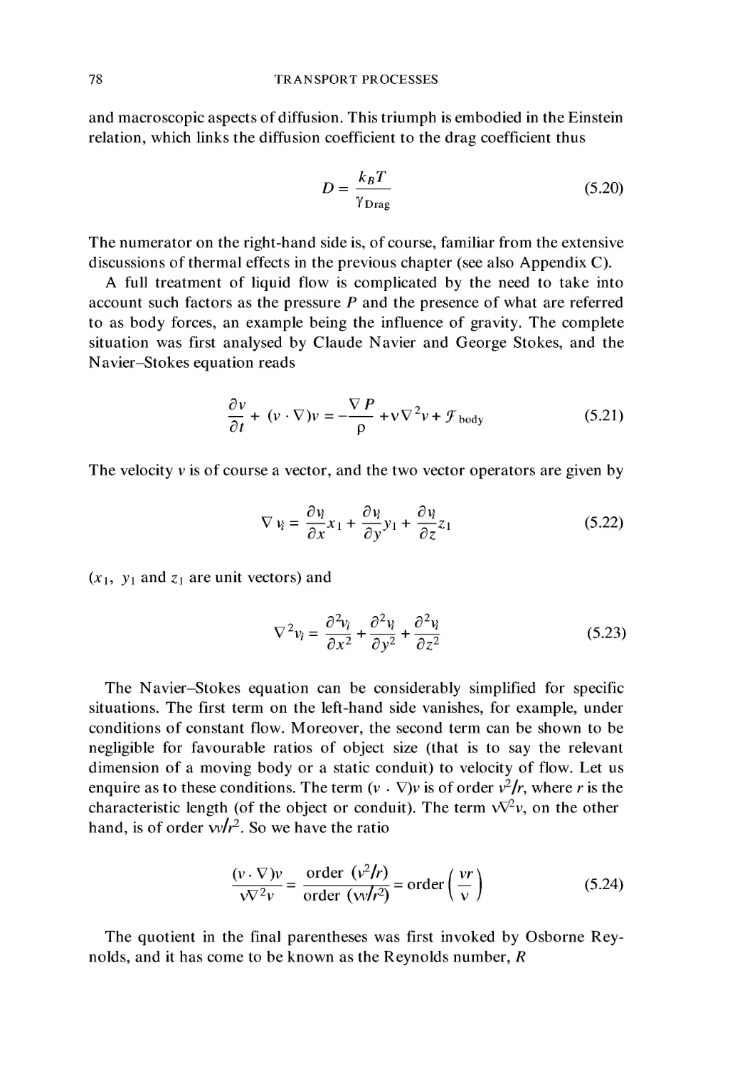
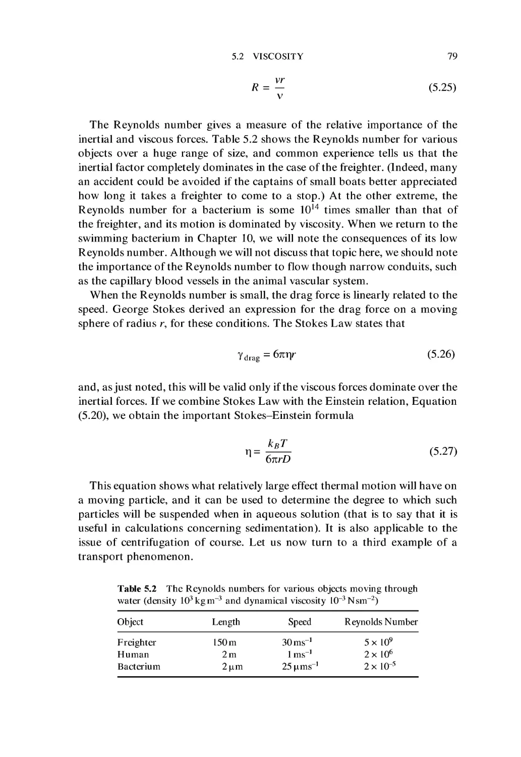
5.2 Viscosity 76
5.3 Thermal Conduction 80
Exercises 81
Further reading 81
6 Some Techniques and Methods 83
6.1 X-Ray Diffraction and Molecular Structure 83
6.2 Nuclear Magnetic Resonance 93
6.3 Scanning Tunnelling Microscopy 98
6.4 Atomic Force Microscopy 101
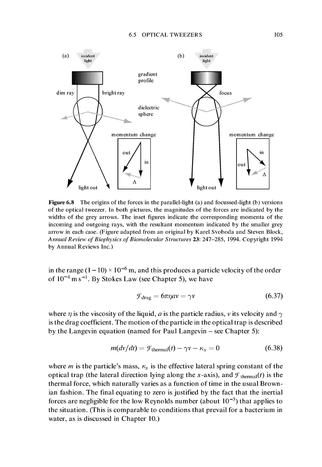
6.5 Optical Tweezers 103
6.6 Patch Clamping 108
6.7 Molecular Dynamics 112
6.8 Potential Energy Contour Tracing 115
Exercises 118
Further reading 119
7 Biological Polymers 123
7.1 Nucleic Acids 124
7.2 Nucleic Acid Conformation: DNA 129
7.3 Nucleic Acid Conformation: RNA 132
7.4 Proteins 134
7.5 Protein Folding 151
Exercises 157
Further reading 158
8 Biological Membranes 161
8.1 Historical Background 161
8.2 Membrane Chemistry and Structure 166
8.3 Membrane Physics 174
Exercises 185
Further reading 185
9 Biological Energy 187
9.1 Energy Consumption 187
9.2 Respiration 188
9.3 Photosynthesis 190
9.4 ATP Synthesis 199
Exercises 206
Further reading 207
10 Movement of Organisms 209
10.1 Bacterial Motion 209
10.2 Chemical Memory in Primitive Organisms 218

CONTENTS ix
10.3 Muscular Movement 220
10.4 Human Performance 233
Exercises 235
Further reading 235
11 Excitable Membranes 237
11.1 Diffusion and Mobility of Ions 237
11.2 Resting Potential 240
Exercises 246
Further reading 246
12 Nerve Signals 249
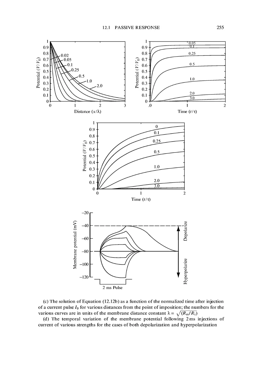
12.1 Passive Response 249
12.2 Nerve Impulses (Action Potentials) 256
12.3 The Nervous System 268
Exercises 275
Further reading 275
13 Memory 277
13.1 Hebbian Learning 277
13.2 Neural Networks 281
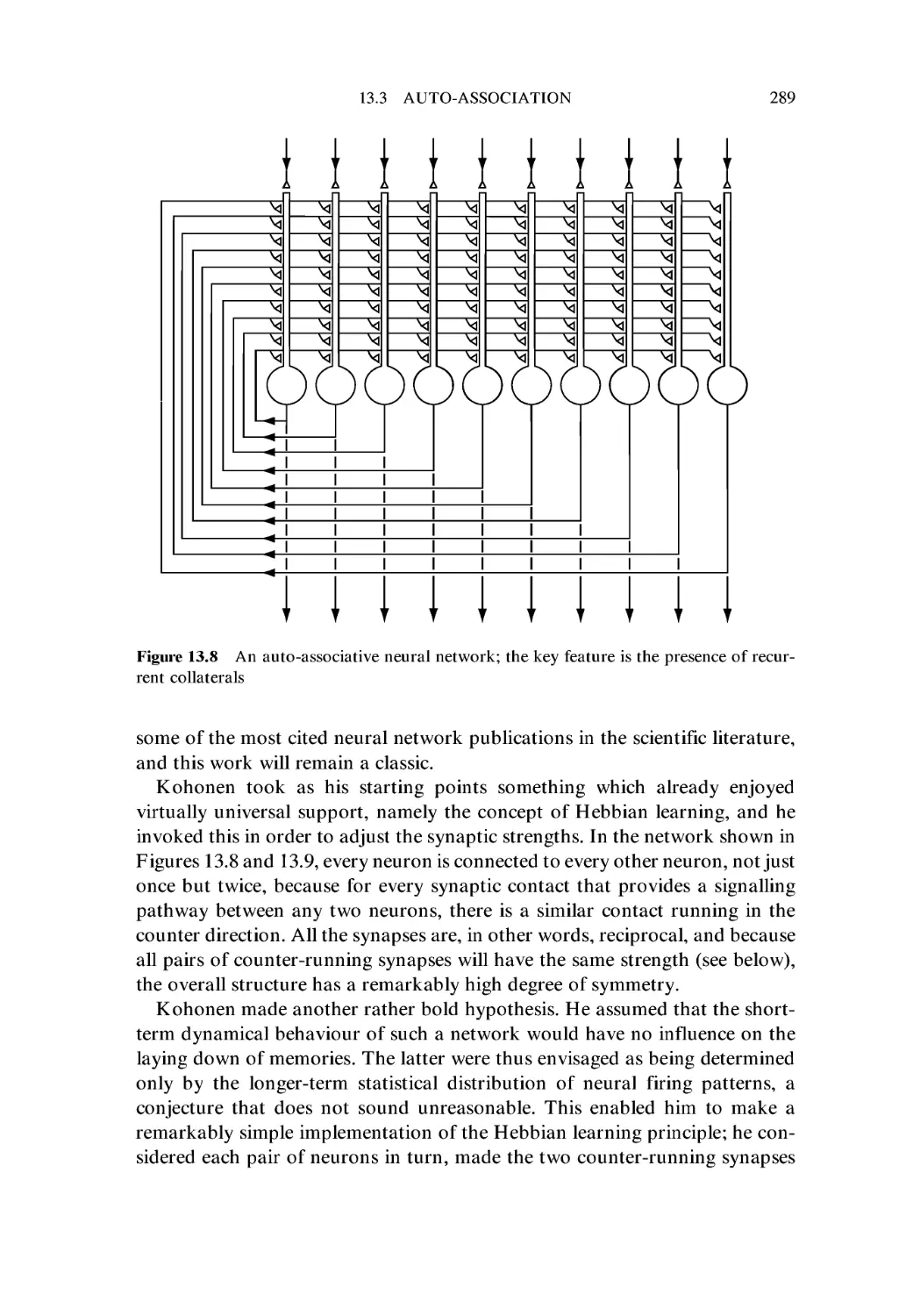
13.3 Auto-association 288
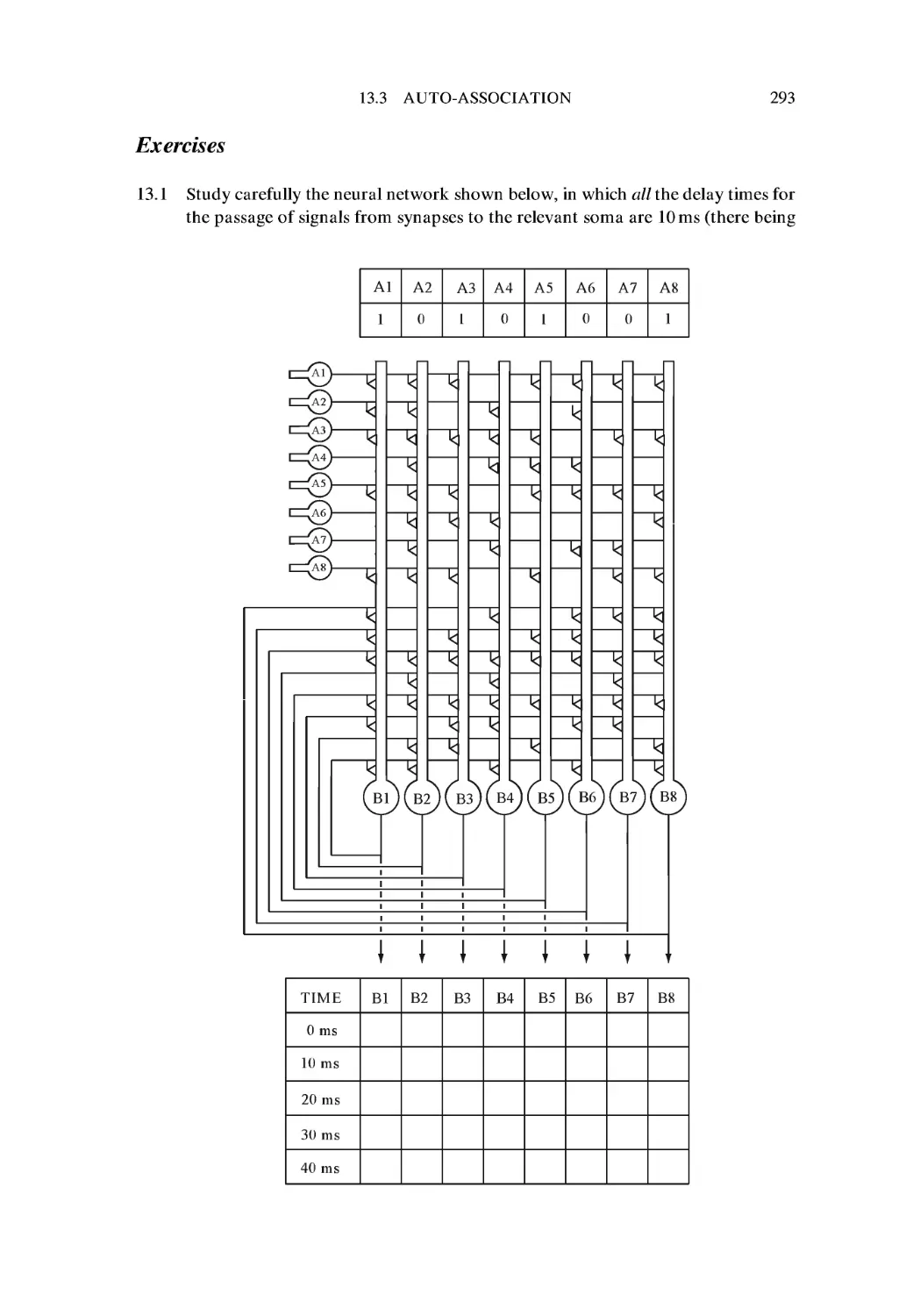
Exercises 293
Further reading 294
14 Control of Movement 297
14.1 The Primacy of Movement 297
14.2 Ballistic Control in a Simplified Visual System 299
14.3 More Sophisticated Modes of Control 304
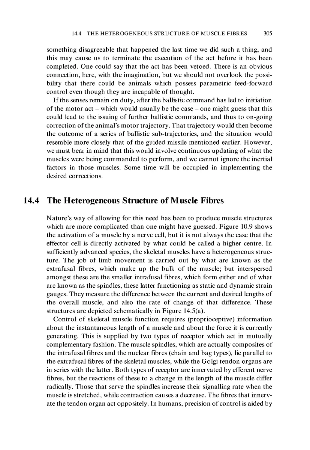
14.4 The Heterogeneous Structure of Muscle Fibres 305
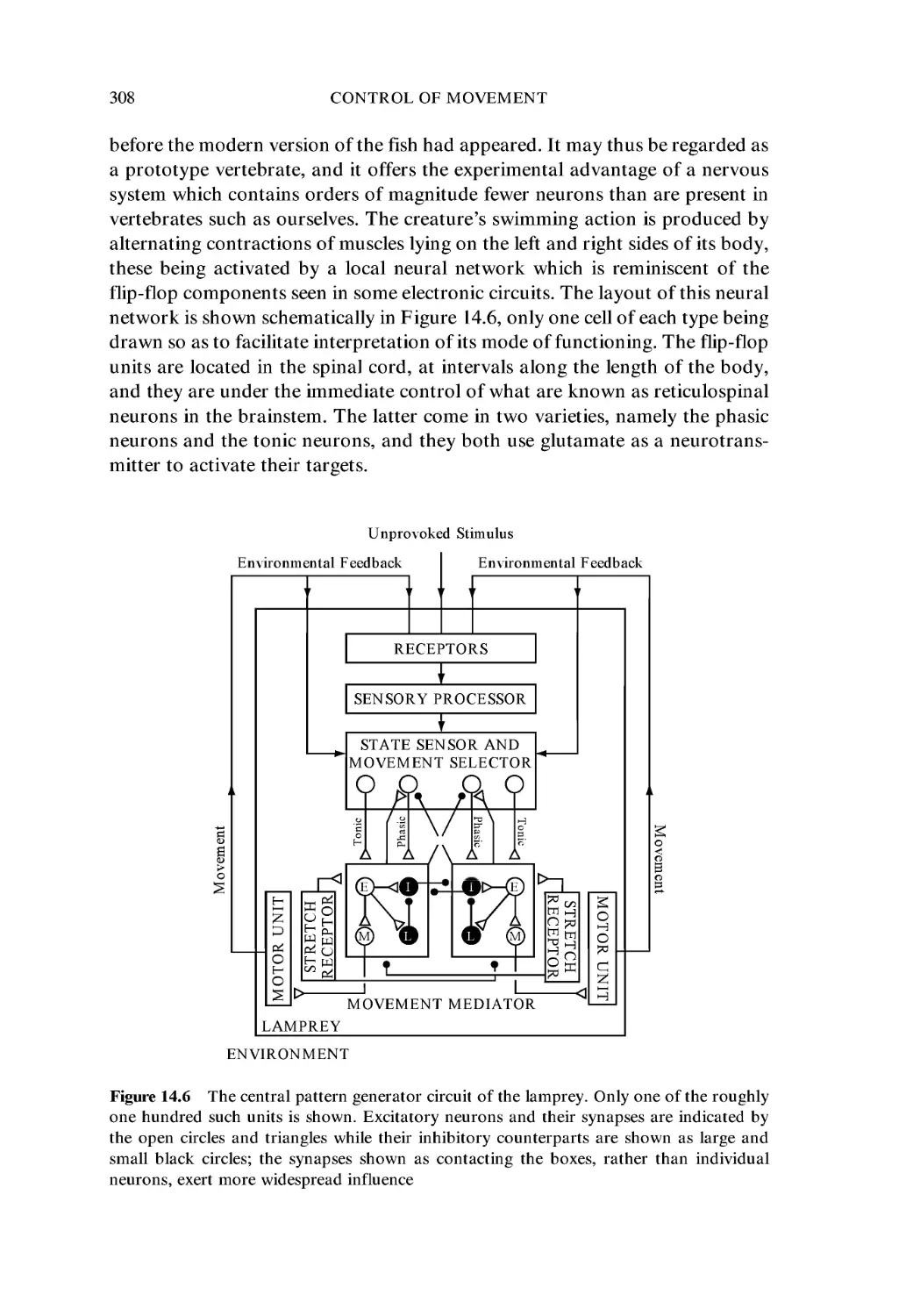
14.5 Central Pattern Generators 307
14.6 Conditioned Reflexes 311
14.7 Volition and Free Will 314
14.8 What Purpose Does Consciousness Serve? 320
14.9 Passive versus Active in Mental Processing 325
14.10 The Relevant Anatomy and Physiology 328
14.11 Intelligence and Creativity 335
14.12 A Final Word 338
Exercises 339
Further reading 339
Appendix A: Elements of Quantum Mechanics 343
A.I Quantization of Energy 343
A.2 Atomic Structure 345
A.3 The Wave Equation 347
A.4 Quantum Mechanical Tunnelling 350

x CONTENTS
Exercises 352
Further reading 352
Appendix B: The Hydrogen Atom 353
B.I The Hamiltonian 353
B.2 The Hydrogen Atom 353
B.3 Solution of the Ф Equation 356
B.4 Solution of the 0 Equation 357
B.5 Solution of the R Equation 358
B.6 Quantum Numbers and Energy Levels 360
B.7 Wave Functions 360
Exercises 364
Further reading 364
Appendix C: Thermal Motion 365
C.I Ideal Gases 365
C.2 Liquids 369
Exercises 371
Further reading 371
Appendix D: Probability Distributions 373
D.I Bernoulli Trials and the Binomial Distribution 373
D.2 The Poisson Approximation 373
D.3 The Normal, or Gaussian, Distribution 375
Further reading 376
Appendix E: Differential Equations 377
Further reading 379
Name Index 381
Subject Index 385

Preface
This book is based on the course in biophysics that I have taught for the past
two decades at the Danish Technical University, and it should be suitable for
similar courses at other places of higher education.
I originally delivered the lectures in Danish and Henrik J0rgensen, one of my
first students, recorded my words in shorthand and then collaborated with my
secretary, Carolyn Hallinger, to produce a set of Danish notes. I updated these
from time to time, and ultimately translated them into English. There were two
subsequent expansions of the text before it acquired the form reproduced here.
Meanwhile Ove Broo S0rensen and Bj0rn Nielsen provided valuable help with
many of the illustrations.
The course now attracts so many students that 1 have needed the backing of
two assistant teachers, in connection with the weekly homework assignments.
Henrik Bohr and Bj0rn Nielsen have provided this service with great skill and
diligence, and it is a pleasure to acknowledge their contribution to the enterprise.
The cause of biophysics at this university has benefited greatly from the
support provided by colleagues in other departments, and most notably by
Robert Djurtoft, Ole Mouritsen, Knud Saermark and Jens Ulstrup, together
with whom I set up what came to be known as the Biophysics Initiative.
Professors Mouritsen and Saermark were formerly my departmental col-
colleagues, and I enjoyed close interactions with both of them.
The interest and encouragement of the wider Danish biophysics community
has also been invaluable, and I would especially like to mention Salim Abdali,
Preben Alstr0m, Olaf Sparre Andersen, Svend Olav Andersen, Christen Bak,
Per Bak, Rogert Bauer, Klaus Bechgaard, Kirstine Berg-S0rensen, Myer
Bloom, Jacob Bohr, Tomas Bohr, John Clark, Jens Peder Dahl, Tom Duke,
Henrik Flyvberg, Christian Fr0jaer-Jensen, Sonia Grego, John Hjort Ipsen,
Karl Jalkanen, Mogens H0gh Jensen, Kent J0rgensen, Carsten Knudsen,
Bent Kofoed, Morten Kringelbach, Erik Hviid Larsen, Signe Larsen, Jens
J0rgen Led, Per Anker Lindegaard, Jens Ulrik Madsen, Axel Michelsen, Erik
Mosekilde, Knud M0rch, Claus Nielsen, Simon N0rrelykke, Lene Oddershede,

xii PREFACE
Niels Berg Olsen, Steffen Petersen, Flemming Poulsen, Christian Rischel, Jens
Christian Skou, Kim Sneppen, Ove Sten-Knusen, Maria Sperotto, Stig
Steenstrup, Thomas Zeuthen and Martin Zuckerman.
Solutions for the exercises can be found on my website:
http://info.fysik.dtu.dk/Brainscience/rodney.html
Rodney Cotterill

Introduction
It is probably no exaggeration to say that many regard biophysics as a discip-
discipline still waiting to be adequately defined. This conclusion appears to be
endorsed by the considerable differences between several of the publications
on the subject cited at the end of this chapter. Indeed, in terms of the items they
discuss, these barely overlap with each other. But this should be taken as an
indication of the sheer multiplicity of things that now belong under the bio-
biophysics banner; no single author could reasonably be expected to cover them
all. If one considers what these books and articles describe collectively, a
unified picture does in fact emerge.
Biophysics is simply the application of physics to biology, with a view to
furthering the understanding of biological systems. There is a related activity in
which methods developed originally for purely physical challenges have been
applied to biological (and in some cases medical) issues. Biophysics tends to be
studied by those who have a background in physics, and who may thus be
bringing useful expertise to the investigation of living things. But there have
also been examples of biologists acquiring the requisite knowledge of physics
and then using this to solve a specific problem.
Biophysics is not a young subject, but its emphasis has gradually changed
over the years. In the first part of the 20th century, biophysicists primarily
concerned themselves with things quite closely related to medicine, and many
large hospitals had a resident member of this fraternity. The issues of interest
were the flow of blood through pumps and the associated tubing (drawing on
the work of George Stokes, among others), the monitoring of heart function
through the related electrical activity, and later of brain activity with much the
same instrumentation (with valuable input from Hans Berger), and also the
fracture of bone (with a borrowing of the ideas developed by Alan Griffith, in a
quite different context).
Around the same time, the field was gradually acquiring a new type of
activity related to processes at the atomic level, this having been provoked by
Wilhelm Rontgen's discovery of X-rays. His astonishment at discovering their
power of penetrating human tissue, but apparently not bone, soon led to the
use of X-rays for diagnostic purposes, of course. Only later did it emerge that
there are grave dangers associated with such radiation, and physicists then

2 INTRODUCTION
found their advice being sought in connection with the monitoring of X-ray
doses. Through their efforts, recording by film was supplemented by recording
with electronic devices. One of the pioneering theoretical efforts in understand-
understanding the interaction of radiation with matter was published by Niels Bohr, who
had earlier put forward the first successful picture of the atom.
These developments were of obvious importance to medicine, but another
use of X-rays, originally confined to the inorganic domain, was later going to
have an enormous impact on all of biology, and through this on medicine itself.
Max von Laue and his colleagues, Walter Friedrich and Paul Knipping, had
discovered the diffraction of X-rays, and William Bragg and Lawrence Bragg
were soon applying the phenomenon to the determination of crystal structures.
The latter Bragg, William's son, encouraged the extension of the technique to
the biological realm, and researchers such as William Astbury, John Bernal,
Peter Debye and Max Perutz soon took up the challenge. The early work in the
area, before the Second World War, contributed to the determination of the
sizes of protein molecules, and within twenty years it was producing pictures of
proteins at the atomic level.
Mention of molecular size serves as a reminder that it would be easy to
overlook the importance of methods developed for separating different molecu-
molecular species, and their consequent contribution to biology. These methods would
not have emerged had it not been for the prior work on the underlying physics.
So the development of techniques such as ultra-centrifugation (invented by The
Svedberg), electrophoresis (by Arne Tiselius) and partition chromatography (by
Archer Martin and Richard Synge) owes much to the earlier efforts of George
Stokes, Albert Einstein and Irving Langmuir.
But to return to structure determination by means of X-ray diffraction, this
approach reached its zenith around the middle of the 20th century. Max Perutz
and John Kendrew set about determining the structures of the oxygen-
transporting proteins myoglobin and its larger cousin haemoglobin. Meanwhile,
Maurice Wilkins, Rosalind Franklin and Raymond Gosling had turned their
attention to deoxyribonucleic acid (DNA). Within a decade, the secrets of these
key structures had been exposed, important input having come from the know-
knowledge acquired of the bonding between atoms, thanks to the efforts of physicists.
Another spectacular success for physics was the invention of the electron
microscope by Ernst Ruska (following important efforts by Denis Gabor).
This played a vital role in the study of the micro structure of muscle, by Hugh
Huxley and his colleagues, and of viruses, by Aaron Klug and Robert Home,
and their respective colleagues. And there was still good mileage to be had from
X-rays because Allan Cormack and Godfrey Hounsfield applied these to the
study of brain tissue, by computer assisted tomography (CAT scanning). This
fine lead was subsequently augmented by development of such other brain-
probing techniques as positron emission tomography (PET) and functional
magnetic resonance imaging (fMRI). And while on the subject of the brain, we

INTRODUCTION 3
have magnetoencephalography (MEG), which owes its existence to something
which started as speculation in the purest of physics, namely the work of Brian
Josephson on quantum mechanical tunnelling between superconductors.
So the current growth in the application of physics to biology can point
to many respectable antecedents. To the names already quoted of physicists
who turned their talents to biology we could add Francis Crick (who has
latterly shifted his attention from matters molecular to matters mental), Max
Delbriick, Walter Gilbert, Salvador Luria and Rosalyn Yalow. These research-
researchers, and many others like them, have brought to biology the quantitative
discipline that is the hallmark of physics.
But we should not overlook the unwitting contributions to biology made by
physicists of an earlier era - physicists who had probably never even heard of
the word biophysics. And in this respect, no advance can quite compete with
that which came from the seemingly esoteric study of gaseous discharge. In
1855, Heinrich Geissler devised a vacuum pump based on a column of mercury
which functioned as a piston. He and Julius Plticker used this to remove most
of the air from a glass tube into which they had sealed two electrical leads, and
they used this simple apparatus to study electrical discharges in gases. Their
experiments, and related ones performed by Michael Faraday and John Gas-
siot, probed the influences of electric and magnetic fields on the glow discharge,
and it was established that the light was emitted when 'negative rays' struck the
glass tube. The discharge tube underwent a succession of design modifications,
by William Crookes, Philipp Lenard and Jean Perrin, and this activity culmin-
culminated with Wilhelm Rontgen's discovery of X-rays in 1895 and Joseph (J. J.)
Thomson's discovery of the electron, two years later. These landmarks led,
respectively, to the investigations of atomic arrangement mentioned above,
and explanations of the forces through which the atoms interact.
These advances were to prove pivotal in the study of biological systems.
Moreover, we should not overlook the instruments that owe their existence to
those early investigations of the influences of various fields on an electron beam.
These led to the cathode ray oscilloscope, with which Edgar Adrian was able to
discover the all-or-nothing nature of the nerve impulse. The precision with
which that instrument enables one to determine the temporal characteristics
of the impulse was vital to Alan Hodgkin and Andrew Huxley's explanation of
nerve conduction. The cathode ray oscilloscope presaged the emergence of
electron microscopy, which was referred to above.
We should add one more name to the list, because it is nearly always
overlooked: John Atanasoff. In the 1930s, confronted with a data analysis
problem in his research in solid-state physics, he hit upon the idea of automat-
automating his calculations with an electronic machine. This was, indeed, the first
electronic digital computer, and the descendants of that device have been
indispensable to many of the techniques mentioned above. It would not be
eccentric, therefore, to call Atanasoff one of the unsung heroes of biophysics.

4 INTRODUCTION
Biophysics, then, is an activity that operates within biology, and it contrib-
contributes to the tackling of some of the major mysteries in that realm. Even though
there may be some dispute as to which are the main issues at the current time,
few would dispute the claim that protein folding, tissue differentiation, speci-
ation, microscopic recognition and (not the least) consciousness and intelli-
intelligence are amongst the greatest challenges of our era. It is certainly the case that
when we fully understand the physical principles underlying these phenomena,
biology as a whole will be very much more advanced than it is today.
Let us briefly consider the nature of these challenges. First, the protein-
folding problem has been referred to as the second half of the genetic code. It
has long been known that the sequence of bases in the DNA molecule deter-
determines the sequence of amino acids in a protein, that is to say the protein's
primary structure. It is also well known that the primary structure dictates
the final three-dimensional conformation of the protein molecule, but we are
unable at the present time to predict that structure, working solely from
the primary sequence. The best that one can do is to predict, with a reasonable
degree of reliability, certain sub-structural motifs that are frequently observed
to be present in the three-dimensional structure. Although this is a notable
achievement in its own right, it still falls far short of the desired ability to
predict any protein's structure from the primary sequence, and this is an
obvious obstacle to full realization of the potential inherent in genetic manipu-
manipulation. If one were able to overcome that hurdle, this would open up the
possibility of tailoring proteins to fulfil specific tasks, for the fact is that what
a protein does is determined by its three-dimensional structure.
The tissue-differentiation problem arises from the fact that every cell in a
multi-cellular organism contains an identical set of genetic instructions, but for
some reason only part of the message is expressed in any one type of cell. In our
own bodies, for example, it is this fact that determines that there are different
cellular structures in our various parts, and that the same distribution of these
bits and pieces is observed in every normal individual. It has long been clear
that the differentiation mechanism depends upon the interaction of proteins
and nucleic acids, and that it thus hinges on the forces between the constituent
atoms. It has also emerged that the differentiation process depends upon the
diffusion of certain molecular species in the growing embryo. Biophysics can
thus contribute to this topic, through elucidating the microscopic factors that
influence the diffusion.
Speciation deals with the questions of why and how a single species occasion-
occasionally gives rise to two distinct evolutionary branches. It has long been clear that
modification of the genetic message lies at the heart of this phenomenon, but the
details are still lacking. After all, no two humans have identical sets of genes
(unless they happen to be clones or identical twins, triplets, etc.), but we never-
nevertheless all belong to the same species. Here, too, interaction between molecules is
of the essence.

INTRODUCTION 5
Microscopic recognition has to do with the molecular processes that dictate
the manner in which different cells mutually interact. Such interactions are
important for all the body's cells, but they are particularly important in the case
of those that belong to the immune system. The great importance of this system
is reflected in the fact that over 1% of a person's body weight is represented by
such cells. They must distinguish between those things that belong to the
body's tissues and outsiders that might threaten the organism's integrity. So,
yet again, one has a mechanism that ultimately depends upon interactions
between atoms.
Finally, there is the great mystery of consciousness and the related issue of
intelligence. Although there are those who prefer to make a clear distinction
between mind and body, there is a growing feeling that it might soon be
possible to understand how such ephemeral things as consciousness and the
mind arise from the physiological processes that occur in the nervous system. It
is by no means clear that adumbration of the physical basis of consciousness
would also further our understanding of what underlies intelligence, but it does
not appear too optimistic to believe that this could be the case.
It might seem that this list of problems overlooks other pressing issues in the
biological domain. One might be tempted to ask why the major scourges of
cancer and AIDS have not been included. The fact is, however, that they
are implicit in two of the above five categories, because cancer is merely one
aspect of the wider issue of tissue differentiation, and AIDS is caused by the
human immune deficiency virus (HIV), which undermines the immune system,
the latter being categorized under the general heading of microscopic recogni-
recognition.
The challenging problems identified above have not been listed in an arbi-
arbitrary order. On the contrary, they show a natural progression from the level of
a single molecule, as in the case of the protein-folding issue, to properties of the
organism that derive from the behaviour of millions of individual cells. In
much the same way, the subject matter in this book follows a logical sequence
in which processes at the atomic level are dealt with first, while relevant
properties of the nervous system appear toward the end of the book. In
between those extremes, the sequence roughly follows that of increasing size.
Thus the discussion of molecules leads on logically to properties of organelles,
and this in turn is followed by a brief treatment of entire cells. Finally, the issue
of neural signalling is discussed, both at the level of the single neuron and
ultimately with reference to the functioning of the entire brain. Important items
in this latter part of the book are membrane excitability, which underlies that
signalling, the changes at the sub-cellular level involved in the laying down of
memories, and the process of cognition. On the other hand, no chapters
specifically address the three central items in the above list. These are neverthe-
nevertheless mentioned in the relevant places, and representative items in the scientific
literature are cited in the Further Reading sections.

6 INTRODUCTION
There are approximately 1012 individual cells in the adult human body.
Hopefully, the following chapters will enable the reader to get a good impres-
impression of the processes which occur on a number of different size scales, and
which lead to the overall functioning of the body. The things described herein
should serve to confirm that the quantitative approach has much to recom-
recommend it when one is trying to work out how the body's component structures
and systems acquire their wonderful functions. Finally, this book aims to
endorse what Philip Anderson noted concerning biological phenomena.
These are ultimately dependent on Nature's fundamental forces, of course,
but the existence of higher levels of organization in living matter implies that
there must also be other laws at work. As one makes the transition to each
higher level of organization, one must anticipate the emergence of new prin-
principles that could not have been predicted on the basis of what was seen at the
lower level.
Exercises
1.1 Write an essay on the following question. Will biophysics become one of the
major scientific disciplines in the 21st century?
1.2 Max Perutz once referred to 1953 as the annus mirabilis of molecular biology.
What did he have in mind?
Further reading
Anderson, P. W., A972). More is different. Science, 177, 393-396.
Cerdonio, M. and Noble, R. W., A986). Introductory Biophysics World Scientific, Singa-
Singapore.
Cotterill, R. M. J., B003). The Material World Cambridge University Press, Cambridge.
Elsasser, W. M., A958). The Physical Foundation of Biology Clarendon Press, Oxford.
Flyvbjerg, H., et al., eds., A997). Physics of Biological Systems: From Molecules to Species
Springer, Berlin.
Glaser, R., B001). Biophysics Springer, Berlin.
Nossal, R. J. and Lecar, H., A991). Molecular and Cell Biophysics Addison-Wesley, Red-
Redwood City, CA.
Parak, F. G., B001). Biological physics hits the high life. Physics World 14A0), 28-29.
Parisi, G., A993). Statistical physics and biology. Physics World, 6, 42^7.
Parsegian, V. A., A997). Harness the hubris: useful things physicists could do in biology.
Physics Today, 23-27, July issue.
Schrodinger, E., A944). What is Life? Cambridge University Press, London.
Setlow, R. B. and Pollard, E. C, A962). Molecular Biophysics. Addeson-Wesley, Reading,
MA.
Sybesma, C, A989). Biophysics: An Introduction Kluwer Academic, Dordrecht.

Chemical Binding
In this chapter, a qualitative account of the electronic structure of atoms will be
given (see Appendices A and B), partly because a mathematically precise
analysis of groups of atoms is still not possible, but mainly because a qualita-
qualitative treatment is usually sufficient to provide an understanding of the way in
which atoms bind together to form molecules. We thus begin by taking a brief
look at an isolated atom.
2.1 Quantum Mechanics
Through his own experimental work on the atomic nucleus, Ernest Rutherford
put forward a picture of the atom in which the heavy nucleus is located at the
centre, while the electrons, discovered by Joseph (J. J.) Thomson, move in
the surrounding space, their characteristic distances from the nucleus being
of the order of 0.1 nm (i.e. a tenth of a nanometer, or 1 Angstrom unit). The
major developments in the theory of atomic structure thereafter were due
to Niels Bohr, who realized that only certain energy states would be permitted
by the quantum principle postulated by Max Planck in 1900; by Louis de
Broglie, who advocated that a dual attitude be adopted toward sub-atomic
particles, such that they are regarded as simultaneously having both particle
and wave natures (see Appendix A); and by Erwin Schrodinger, whose equa-
equation showed how to derive the allowed states of electrons, both regarding
their permitted energies and their spatial distribution with respect to the
nucleus.
Schrodinger's time-independent equation reads
М-Ч* = / • 4* B.1)
where H is the Hamiltonian operator, (~ is the energy and ¥ is the wave
function, the latter being a function of position with respect to the nucleus.
This equation appears to be remarkably simple, but one must bear in mind that
the Hamiltonian itself will usually be a composite of several terms, while the
wave function will include components describable only in terms of complex

8 CHEMICAL BINDING
numbers. The solution of the Schrodinger equation for the very important case
of the hydrogen atom is given in Appendix B.
Max Born hit upon the correct interpretation of the distribution yielded by
the Schrodinger equation when he suggested that Ч'Т* (where Ч7* is the complex
conjugate of T) gives the probability that an electron will be located at that
position. (For our purposes here, Ч'Ч'* can be regarded as simply being the
square of the amplitude of the wave function.) Just as the vibrations of a (one-
dimensional) guitar string and the (two-dimensional) skin of a drum can be
characterized by a set of numbers which refer to the positions and multiplicity
of the nodal points (i.e. positions where the amplitude is zero), so it is with the
electron probability distribution around a nucleus. Although we need not go
into the details here, different quantum states of an electron in the vicinity of an
atomic nucleus are characterized by different spherical and non-spherical
probability distributions. Although other factors also come into play, as we
will see later, it is the shapes of these distributions that determine the shapes of
the molecules formed when two or more atoms form a reasonably permanent
mutual liaison.
In the case of the one-dimensional guitar string, the situation can be charac-
characterized by a single number, which is related to the number of nodal points
located along the string. In the case of the vibrating skin of a drum, two
different numbers are required in order to fully characterize the situation:
one of these refers to nodal points whereas the other refers to nodal lines
(which may be curved). In the three-dimensional space around an atomic
nucleus, therefore, it is not surprising that three different numbers are required
for a full description of the spatial arrangement of the probability distribution
for each electron, there now being nodal points, nodal lines and nodal surfaces.
It turns out that a further number is required, because the electron possesses
what is known as spin, which is very roughly analogous to the spin of a planet,
as it describes its orbit around the sun. Just as the spin of such a planet may be
either in a left-handed or a right-handed direction, so too the spin of an
electron has one of just two possibilities. The spin quantum number of an
electron is usually designated by the letter s, and the other quantum numbers
by the letters n, /, and m (see Appendix B). Figure 2.1 shows the spatial
distribution of the squared probability amplitude for a number of different
situations which can apply to an electron in orbit around an atomic nucleus.
These are indeed usually referred to as orbitals.
The lowest energy (ground) state for a hydrogen atom, the Is state, is
characterized by a spherically-symmetric wave intensity with a single spherical
nodal surface at infinity. The lowest energy excited state is the 2s, and this has
an additional spherical nodal surface centred on the nucleus. The 2p states,
which have slightly higher energy, have nodal surfaces which pass through the
nucleus. There are three of them, corresponding to the three possible values of
the magnetic quantum number m. States with lobes extending along one of the

2.2 PAULI EXCLUSION PRINCIPLE
Is
Figure 2.1 Spatial distribution of the squared probability amplitude for a number of
different situations which can apply to an electron in orbit around an atomic nucleus
Cartesian axes can be obtained by mixing the three 2p states in the correct
proportions. The insets in Figure 2.1 and later diagrams indicate schematically
the equivalent Bohr orbits.
2.2 Pauli Exclusion Principle
Although we do not need to go into all the details here, there are certain rules
which are useful when considering situations in which there is more than one
electron present in an atom. For a start, no two electrons can be associated with
the same atomic nucleus and have precisely the same values for all four of the
quantum numbers. This is known as the Pauli Exclusion Principle (after Wolf-
Wolfgang Pauli), and it is a particularly potent factor when two similar atoms lie
sufficiently close to one another. Regarding the actual shapes of the orbitals,
the s types all have spherical symmetry, whereas the p types show elongation
along an axis (see Figure 2.1). (The s used to designate one type of orbital
should not be confused with the symbol for the spin quantum number; see
Appendix B.) When all the p orbitals are fully occupied by their permitted
complement of electrons, however, these collectively also display spherical
symmetry. This is particularly noticeable in the noble gas atoms, which indeed
possess only such full shells. Another important property of electron orbitals is

10 CHEMICAL BINDING
that a linear combination of different possible wave functions is also a possible
solution of the time-independent Schrodinger equation.
Suppose that Ti and ¥2 are two such possible wave functions. We will then
have that
and
If we now multiply the first of these equations by the coefficient C\ and the
second by C2, and add the two results, we obtain
#.(Ci-4'i+ C2 -¥2) = ^-(Ci-^i+ С2^2) B.2)
This is an equally valid version of the time-independent Schrodinger equation.
We can now proceed to discuss what happens when two atoms approach
each other. It is clear that they must exert a force upon each other, and a
moment's reflection reveals that these forces may be either attractive or repul-
repulsive. This conclusion comes from the dual facts that matter does not spontan-
spontaneously explode or implode. In other words, one meets with resistance if an
attempt is made to squeeze a piece of condensed matter (i.e. a solid or a liquid)
into a smaller volume. Likewise, resistance is encountered if one tries to stretch
a piece of material beyond its quiescent dimensions. This indicates that the
interatomic potential is repulsive at sufficiently short range and attractive at
sufficiently long range, and the implication is thus that there must be an
intermediate distance at which there is neither repulsion nor attraction. This
will correspond to an interatomic separation for which the forces are precisely
balanced, and it is this characteristic distance that essentially determines the
density of a piece of material.
2.3 Ionization Energy, Electron Affinity and Chemical Binding
It is interesting to note that these considerations were well appreciated even
before it had been unequivocally demonstrated that atoms actually exist. It is
not surprising, therefore, that the arguments do not take into account possible
redistribution of the subatomic particles when two atoms approach one another
sufficiently closely. In general, there will be a rearrangement of the electrons
between the two atoms, the notable exception being the case where both atoms
are of the noble gas type. Two quantities are of importance when considering
what might happen in the two-atom case, these being the ionization energy

2.3 IONIZATION ENERGY AND ELECTRON AFFINITY
11
and the electron affinity. The ionization energy, E\, is the minimum energy
required to remove an electron from an otherwise neutral atom. The situation is
described by
■A+ +
B.3)
A denotes the neutral atom, A+ a positively charged ion, and e the electron.
The electron affinity, EA, is the energy gained when a neutral atom acquires an
additional electron. This other situation is described by
A + e
B.4)
A denotes the negatively charged atom that results from this process. It is very
important to note that these two equations are not merely mutual opposites,
because the product of the first reaction is a positive ion and a negative
electron, whereas the participants in the second reaction are a neutral atom
and a negative electron.
A good example is seen in the compound lithium fluoride, in which a lithium
atom readily donates one of its electrons to a fluorine atom, the latter thereby
acquiring an electron structure which resembles that of a noble gas atom, with
all of its electron orbitals having the maximum number of permitted electrons
(see Table 2. L). The separation of the electron from the lithium atom requires
an amount of energy equal to the ionization energy, E\. When the fluorine
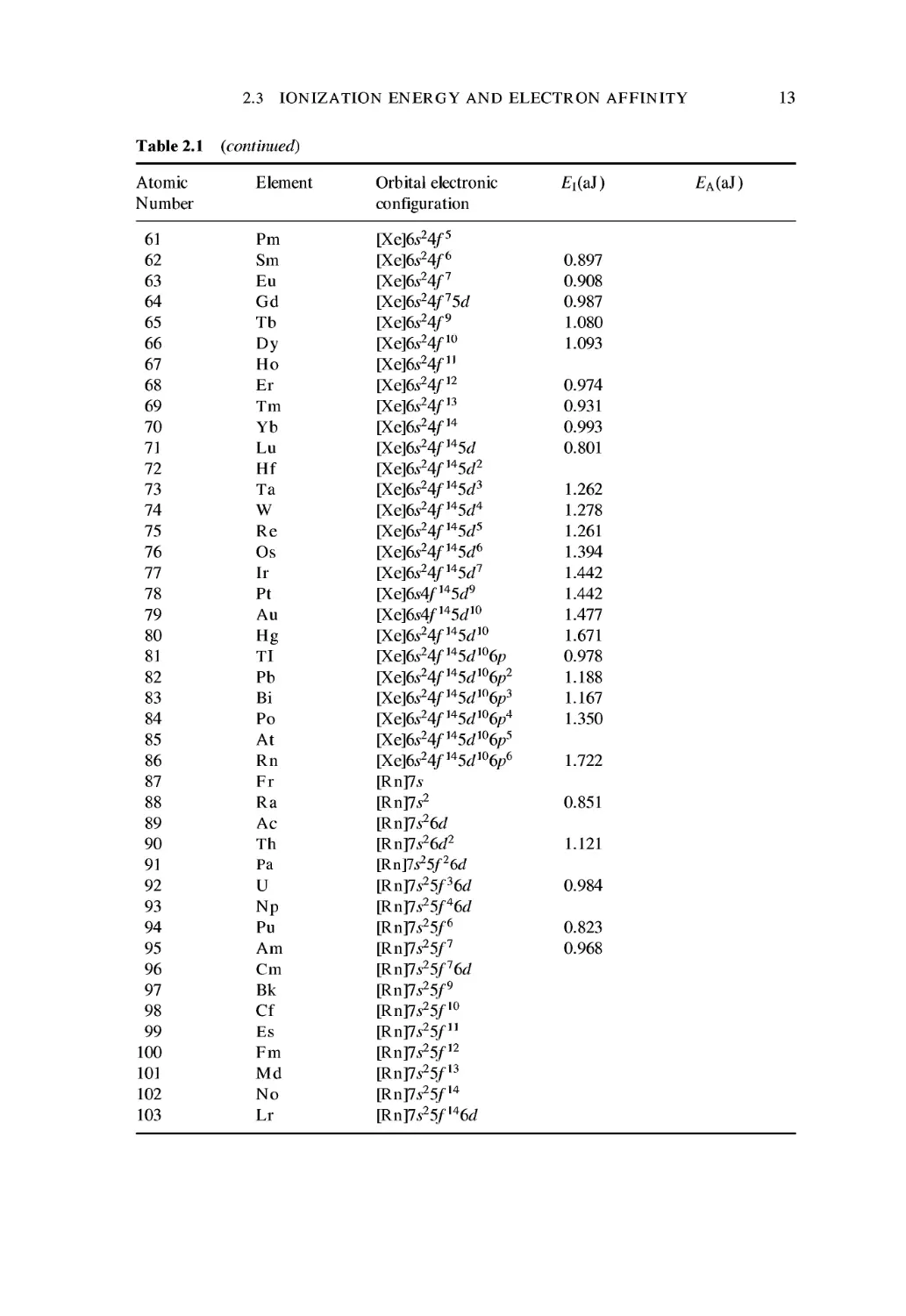
Table 2.1 The electronic characteristics of the elements
Atomic
Number
1
2
3
4
5
6
7
8
9
10
11
12
13
14
15
Element
H
He
Li
Be
В
С
N
О
F
Ne
Na
Mg
Al
Si
P
Orbital electronic
configuration
Is
Is2
\He\2s
\He\2s2
\He]2s22p
\He\2s22p2
\He\2s22p3
\He\2s22p4
\He\2s22p5
\He]2s22p6
\Ne\3s
\Ne\3s2
\Ne\3s23p
\Ne\3s23p2
\Ne\3s23p3
£i(aJ)
2.178
3.938
0.863
1.493
1.329
1.804
2.329
2.181
2.791
3.454
0.823
1.225
0.959
1.305
1.762
£A(aJ)
0.120
0.087
-0.096
0.032
0.200
-0.016
0.235
0.553
0.119
-0.048
0.096
0.261
0.112
continues overleaf

12
CHEMICAL BINDING
Table 2.1 (continued)
Atomic
Number
16
17
18
19
20
21
22
23
24
25
26
27
28
29
30
31
32
33
34
35
36
37
38
39
40
41
42
43
44
45
46
47
48
49
50
51
52
53
54
55
56
57
58
59
60
Element
S
Cl
Ar
К
Ca
Sc
Ti
V
Cr
Mn
Fe
Co
Ni
Cu
Zn
Ga
Ge
As
Se
Br
Kr
Rb
Sr
Y
Zr
Nb
Mo
Tc
Ru
Rh
Pd
Ag
Cd
In
Sn
Sb
Те
I
Xe
Cs
Ba
La
Ce
Pr
Nd
Orbital electronic
configuration
[Ne]3s23p4
\Ne\3s23p5
\Ne\3s23p6
[Ar]4s
[Ar]4s2
[Ar]4s23J
[Ar]4s23J2
[Ar]4s23d3
[Ar]4s3d5
[Ar]4s23d5
[Ar]4s23d6
[Ar]4s23d7
[Ar]4s23d8
[Ar]4s3d]0
[Ar]4s23d10
[Ar]4s23d104p
[Ar]4s23d104p2
[Ar]4s23d104p3
[Ar]4s23d104p4
[Ar]4s23d104p5
[Ar]4s23d1(V
[Kr]5s
[Kr]5s2
[Kr]5s24d
[Kr]5s24d2
[Kr]5s4d4
[Kr]5*4J5
[Kr]5*24J5
[Kr]5s4d7
[Kr]5*4J8
[Kr]4J]0
[Kr]5*4J]0
[Kr]5*24J10
[Kr]5s24d]05p
[Kr]5*24J105p2
[Kr]5*24J]05p3
[Kr]5*24J105p4
[Kr]5*24J'°5p5
[Kr]5s24d]05/
\Xe\6s
\Xe\6s2
\Xe\6s25d
\Xe\6s24f5d
[Xe]6s24/3
\Xe\6s24f4
1.659
2.084
2.524
0.695
0.979
1.051
1.094
1.080
1.083
1.191
1.266
1.259
1.223
1.237
1.504
0.961
1.262
1.572
1.562
1.897
2.242
0.669
0.912
1.041
1.113
1.085
1.137
1.166
1.180
1.195
1.334
1.213
1.440
0.927
1.176
1.384
1.443
1.675
1.943
0.624
0.835
0.899
1.107
0.923
1.011
£A(aJ)
0.332
0.578
-0.144
0.029
0.192
0.096
0.272
0.538
-0.096
0.032
0.352
0.490

2.3 IONIZATION ENERGY AND ELECTRON AFFINITY
13
Table 2.1 (continued)
Atomic
Number
Element
Orbital electronic
configuration
61
62
63
64
65
66
67
68
69
70
71
72
73
74
75
76
77
78
79
80
81
82
83
84
85
86
87
88
89
90
91
92
93
94
95
96
97
98
99
100
101
102
103
Pm
Sm
Eu
Gd
Tb
Dy
Ho
Er
Tm
Yb
Lu
Hf
Та
W
Re
Os
Ir
Pt
Au
Hg
TI
Pb
Bi
Po
At
Rn
Fr
Ra
Ac
Th
Pa
U
Np
Pu
Am
Cm
Bk
Cf
Es
Fm
Md
No
Lr
\Xe\6s4f5
[Xe]6s24/6
[Xe]6s24/7
\Xe\6s24f75d
\Xe\6s24f9
[Xe]6s24/10
\Xe\6s24fn
\Xe\6s24fn
[Xe]6s24/13
\Xe\6s24fu
\Xe\6s24fu5d
\Xe\6s24fu5d2
\Xe\6s24fu5d3
\Xe\6s24fu5d4
\Xe\6s24fu5d5
\Xe\6s24fu5d6
\Xe\6s24fu5d7
\Xe\6s4fu5d9
\Xe\6s4fu5dw
\Xe\6s24fu5di0
\Xe\6s24fu5di06p
\Xe\6s24fu5di06p2
\Xe\6s24fu5di06p3
\Xe\6s24fu5dw6p4
\Xe\6s24fu5di06p5
\Xe\6s24fu5dw6p6
[Rn]7*
\Rn]ls2
\RnJ7s26d
\RnJ7s26d2
[Rn]7^5/26J
\Rn]ls25f36d
\RnJ7s25f46d
\RnJ7s25f6
\Rn]7s25f7
\RnJ7s25f76d
\RnJ7s25f9
\RnJ7s25fiO
\RnJ7s25fn
\Rn]7s25fn
\RnJ7s25fn
\Rn]7s25fu
\RnJ7s25fu6d
0.897
0.908
0.987
1.080
1.093
0.974
0.931
0.993
0.801
1.262
1.278
1.261
1.394
1.442
1.442
1.477
1.671
0.978
1.188
1.167
1.350
1.722
0.851
1.121
0.984
0.823
0.968

14 CHEMICAL BINDING
atom subsequently acquires that same electron, and thereby develops an elec-
electron structure resembling that of neon, the overall system gains an amount of
energy equal to the electron affinity, Ea- Because E\ is usually larger than Ea,
this electron transfer process might seem to require a net input of energy (see
Table 2.2). However, we must remember that the situation does not involve
two atoms that are well separated. On the contrary, they remain in the vicinity
of each other, and so there are other energy contributions to be taken into
account. It transpires that the Coulomb interaction (named for Charles de
Coulomb) fully compensates for the above net energy input, so there will
indeed be chemical binding between the two atoms involved. The situation is
illustrated in Figure 2.2, and one notes that the binding is purely electrostatic in
nature; there is no directionality in the binding. This interaction is, of course, a
classical example of ionic bonding.
In ionic bonding, electropositive and electronegative atoms combine through
the electric attraction between ions that are produced by electron transfer. Good
examples are provided by the alkali halides such as LiF. Each neutral (electro-
(electropositive) lithium atom loses its 2s electron and thereby becomes a positive ion,
somewhat resembling a positively-charged helium atom. Each neutral (electro-
(electronegative) fluorine atom gains an extra 2p electron and becomes a negative ion,
resembling a negatively-charged neon atom.
It is no coincidence that it is the lithium atom in the above reaction that loses
an electron. Of the two elements involved, it is lithium that has a lone electron
outside shells that are fully occupied. The fluorine atom, on the other hand, has
an outermost shell that lacks only one electron. This difference is clearly revealed
in the first ionization energies of the two atoms (that is to say the energy which
must be expended in removing one electron from the neutral atom). As can be
seen in Table 2.1, the first ionization energy of lithium is 0.863 aJ, whereas
the first ionization energy of fluorine is 2.791 aJ. Indeed, to find ionization
Table 2.2 Comparison of electronegativity
with the sum of ionization energy and
electron affinity. All values are for 25°C
F
Cl
Br
I
H
Li
Na
К
Rb
Cs
Ei
2.8
2.1
1.9
1.7
2.2
0.9
0.8
0.7
0.7
0.6
EA
0.6
0.6
0.5
0.5
0.1
0.1
0.1
0
0
0
Sum
3.4
2.7
2.4
2.2
2.3
1.0
0.9
0.7
0.7
0.6
eN
4.0
3.0
2.8
2.5
2.1
1.0
0.9
0.8
0.8
0.7

2.4 ELECTRONEGATIVITY AND STRONG BONDS
15
neutral
Li atom
3 protons
3 electrons
Li4 ion
neutral
F atom |
9 protons
9 electrons = Is22s22p22p22pj
F~ ion I
electron
transfer
3 protons
2 electrons = Is2
9 protons
10 electrons = Is22s22p22p22pf N
electric attraction
Figure 2.2 An illustration of ionic bonding in the case of LiF
energies larger than that exhibited by the fluorine atom, one would have to go
to the noble gases themselves, with their fully occupied electron orbitals.
2.4 Electronegativity and Strong Bonds
Although the propensity that a given atomic species displays for losing or
gaining electrons is determined by the dual factors of ionization potential
and electron affinity, an adequate qualitative measure of the same thing is
provided by a single parameter known as the electronegativity, eN. Atoms with
large electronegativities tend to capture electrons, whereas the opposite is the
case for atoms with small electronegativities (these being said to be electroposi-
electropositive). A reliable scale of electronegativity has been derived by Linus Pauling
and it is, as indicated above, a dual measure of ionization energy and electron
affinity. Typical values are given in Table 2.2.

16
CHEMICAL BINDING
If the difference in the electronegativities of two atoms is quite small, there
will be no clear tendency for one to lose an electron while the other gains this
subatomic particle. There is thus no basis for ionic binding in such a situation.
Instead, one has either covalent bonding or metallic bonding, the first of these
occurring if the two atoms are both electronegative, and the latter arising when
they are both electropositive. An example of covalent bonding is seen if the two
atoms involved are both fluorine. The nine electrons in an atom of this element
are arranged in such a way that there are two in the Is orbital, two in the 2s
orbital, two in each of the 2px and 2py orbitals, and finally a single electron in
the 2pz orbital. It is only the latter orbital, therefore, which lacks an electron
and, as we saw in the case of ionic bonding, it can fulfil this need by acquiring
an electron from another atom. However, in the case of the covalent bond, it
does this not by completely removing an electron from that other atom, but
rather by entering into a mutual sharing of atoms, in which the unfilled orbitals
of both atoms are filled by the other's lone 2pz electron.
One sees from Figure 2.3, which depicts the situation in a hydrogen fluoride
molecule, that the 2pz orbitals alone are involved in the binding. Although the
interatomic bond is highly directional, as mentioned earlier, it possesses rota-
rotational symmetry and there is very little resistance to rotation of one of the
atoms with respect to the other, about the z-axis. This form of covalent
bonding is known as a a-bond (sigma bond) and numerous examples are
neutral
H atom
neutral
F atom
0
Is1
Figure 2.3 A simple example of covalent bonding which occurs in the HF molecule

2.4 ELECTRONEGATIVITY AND STRONG BONDS
17
encountered in molecules having biological relevance. In the case of the HF
molecule the incomplete orbitals, the is of hydrogen and the 2p of fluorine,
overlap and the two electrons are shared by a sigma-bond.
If we turn to an atom which lies one place lower in the periodic table, namely
oxygen, it will lack a total of two electrons from its p orbitals rather than just
the one seen in the case of fluorine. In much the same way as before, two
oxygen atoms can form a molecule, and the 2pz orbitals will again overlap,
producing a sigma bond. However, this leaves the 2py orbitals still incompletely
filled, and they can be imagined as bending toward each other so as to produce
further covalent bonding, as seen in Figure 2.4. The latter involves distortion
neutral
О atom
neutral
О atom
electron sharing - a bond of p orbitals
further electron sharing -
n bond of p^, orbitals
Figure 2.4 The covalent bonding between two oxygen atoms involves both a sigma-bond
and a pi-bond

18 CHEMICAL BINDING
Relative Potential Energy Vs. Rotation Angle in pi-bond
90 180 270 360
Rotation Angle
Figure 2.5 An energy versus rotation angle plot of the pi-bond caused by the resistance to
rotation
and overlap of the 2py orbitals and confers axial rigidity on the molecule.
Unlike the case of the sigma bond, with its single overlap along the z-direction,
this new bond will involve two lobes, neither of which lies on that axis. There
will thus now be a two-fold symmetry to the situation, and one can imagine any
attempt to rotate one of the atoms with respect to the other encountering
resistance, due to the fact that the 2py orbitals would thereby be stretched.
This new type of bond is known as a тг-bond (pi bond), and the resistance to
rotation is reflected in an energy versus rotation angle plot which is roughly
sinusoidal, as seen in Figure 2.5.
Four a-bonds are present in the methane molecule, CH4, each one attaching
a hydrogen atom to the central carbon atom. The tetrahedral shape of this
molecule might seem surprising, given what has been said so far about the
mutual orientations of the various/» orbitals (see Figures 2.1 and 2.3), lying at
right angles to one another. The explanation lies in two factors, namely electron
promotion and wave function hybridization. The first of these is viable when the
increase of energy involved in promoting an electron to a higher quantum state
is less than the subsequent lowering of energy when the wave functions can then
be hybridized. Any combination of wave states in an atom is itself a possible
wave state and the result is known as a hybrid orbital. The number of the latter
must equal the number of original orbitals. Thus an s orbital and a p orbital
produce two different sp hybrids (Figure 2.6). The combination of the different
hybrids produces a configuration whose geometry determines the spatial ar-
arrangement of interatomic bonds. The hybridization principle is captured by
Equation B.2). In the case of the methane molecule, CH4, one of the 2s electrons
is promoted to an otherwise-empty 2p state, and the resulting three 2p orbitals
and the one remaining 2s orbital hybridize to produce four sp3 hybrids (see
Figure 2.7). It is the latter which produce the four sigma-bonds

2.4 ELECTRONEGATIVITY AND STRONG BONDS
19
s orbitals
sp hybrid
p orbitals
sp2 hybrid
sp hybrid orbitals
Figure 2.6 Wave function hybridization
sp3 hybrid
methane
Figure 2.7 Hybridization in the methane molecule, CH4
with the Is orbitals of the hydrogen atoms, giving the methane molecule its
tetrahedral symmetry. A somewhat related example is seen in the water mol-
molecule, H2O, (see Figure 2.8). The dominant factor determining the shape of
the water molecule is the hybridization of the 2s and 2p orbitals of the oxygen
atom. The four hybrid orbitals have lobes which project out from the
oxygen nucleus in the direction of the four corners of a tetrahedron. Two of
these orbitals provide bonds for the two hydrogen atoms, while the remaining
two become 'lone-pair' orbitals. The latter are negatively charged and attract the
hydrogen atoms on neighbouring water molecules.

20 CHEMICAL BINDING
Figure 2.8 Hybridization in the water molecule, H2O
Although the energy barrier represented by a тг-bond is not insuperable,
given sufficient thermal or mechanical activation, this type of bond can be
regarded as giving a molecule considerable stiffness at its location. In effect,
this decreases the number of parts of the molecule that are able to move freely,
and in some cases it considerably reduces the alternative conformations that
must be investigated by those who wish to determine molecular structure from
first principles. We will return to such computations later, when considering
the very important protein-folding problem.
In those cases where all atoms present are electropositive, the tendency will
be for a metal to be produced. If the number of atoms is sufficiently large, the
result will be an assembly of positive ions, held together by a sort of glue of
relatively free electrons. The word relatively is important here, however, be-
because in practice the electrons are able to move only with those energies
consistent with the scattering and interference effects that arise because of
their wave nature. This produces the well-known energy bands that are import-
important in distinguishing metals from semiconductors and insulators. Such atomic
assemblies are of relatively minor importance in the biological sphere, how-
however, so we will not discuss them further. All the types of bond discussed so far,
that is to say the ionic, covalent and metallic types, are collectively referred to
as strong bonds. It should be noted that these distinctions are not rigid, and that
many assemblies of atoms display binding that is intermediate between two of
the above-mentioned categories.

2.5 SECONDARY BONDS 21
2.5 Secondary Bonds
Because there exist forms of condensed matter comprising assemblies of mol-
molecules that retain their individual identity, there must be types of intermolecu-
lar force that we have not yet considered. These are known as secondary bonds
and they are quite weak compared with those that we have considered until
now. In those cases where the molecules have no permanent dipole moment
(that is to say, there is no net separation of opposite electrical charges, analo-
analogous to the separation of north and south poles in a permanent magnet), the
most important type of secondary bond is that which is named after Johannes
van der Waals. This type of bond arises because although the atoms involved
have no permanent dipole moments, there are small instantaneous dipole
moments that arise from the motions of the individual electrons. At any
instant, an electron's distribution with respect to the nucleus need not neces-
necessarily be as uniform as is its averaged value, and this means that there will be
instantaneous dipole moments. These can influence those of the surrounding
atoms, and the net outcome can be shown to be a weakly positive attraction
(see Chapter 3). Unlike the covalent bond, this van der Waals bond is not
directional, and it cannot be saturated; the number of other atoms which can
be attracted to a given atom, via the van der Waals force, is determined solely
by geometrical considerations. This is why the crystalline forms of the noble
gases, which enter into only this type of bond, are usually close-packed.
The other type of secondary bond that we need to consider here is the
hydrogen bond, and its importance in biological structures could hardly be
exaggerated. It frequently arises through the interaction of hydrogen and
oxygen atoms, as in the configuration NH ••• ОС. The electronegativity of
the nitrogen atom is so large compared with that of the hydrogen that the
hydrogen atom's lone electron tends to spend most of its time between the two
atomic nuclei. This means that the (proton) nucleus of the hydrogen atom is
not so well screened by the electron as it would be in the isolated neutral version
of that atom. The net result is that the hydrogen atom develops a positive pole.
Just the reverse happens in the case of the oxygen atom, the electronegativity of
which is greater than that of the carbon atom, so it, in turn, functions as a
negative pole. The hydrogen bond is not very strong, but it is quite directional,
in that the nucleus of the hydrogen atom is exposed only within a limited solid
angle. Moreover, the small size of the hydrogen atom limits the number of
other atoms that can approach it sufficiently closely. The hydrogen bond is
thus also quite saturated.
Following this brief and qualitative discussion of the various types of inter-
interatomic bond, we should now turn to the quantitative aspects of interatomic
interactions. These forces dictate the spatial arrangement of the atoms in a
molecule. If we wish to make calculations on the relative stabilities of various
candidate conformations, therefore, we will need a quantitative description of

22 CHEMICAL BINDING
these forces. It is thus to this aspect of the issue that we will turn in the next
chapter.
Exercises
2.1 The atoms of the first five elements of the periodic table contain one (hydrogen),
two (helium), three (lithium), four (beryllium) and five (boron) electrons, respec-
respectively. Using dots to symbolize the nuclei of one atom of each of these five
elements, draw the approximate distributions of electron probability density
corresponding to the lowest energy states of each of these elements.
2.2 Describe the difference between ionization energy and electron affinity.
2.3 Draw the electronic configurations of a a-bond and а л-bond, respectively,
between two appropriate atoms.
2.4 Draw the approximate distributions of electron probability density correspond-
corresponding to the lowest energy state of the nitrogen molecule, N2. Indicate all the
electrons in the molecule, and add labels to indicate the types of bond involved.
2.5 The 1976 Nobel Prize in chemistry was awarded to William Lipscomb for his work
on boranes, which are composed of atoms of boron and hydrogen. From your
knowledge of atomic and molecular orbitals, what would you expect to be the spatial
configuration of the nuclei and electron probability densities in one (or more) of
these boranes, given that they are rather unstable and chemically highly reactive?
Further reading
Atkins, P. W., A990). Physical Chemistry. Oxford University Press, Oxford.
Moore, W. J., A972). Physical Chemistry. Longman, London
Pauling, L., A960). The Nature of the Chemical Bond. Cornell University Press, Ithaca, NY.
Pauling, L., A970). General Chemistry. Freeman, San Francisco.
Serway, R. A., A992). Physics for Scientists and Engineers. Saunders, Philadelphia.

Energies, Forces and Bonds
The discussion in the previous chapter provided the basis for a qualitative
understanding of the factors that influence the interactions between atoms.
And it showed how consideration of the shapes of electron probability orbitals
can lead to an understanding of the three-dimensional shapes of molecules. If
one needs quantitative information about these interactions, however, it is
necessary to have information about the actual forces through which the
various atoms (and indeed molecules) interact. And such information will
include facts about both the analytical forms of particular interatomic inter-
interactions and the relevant parameters. This will be our primary concern in the
present chapter, for we will be considering several well-known interatomic
potential functions, as well as the magnitudes of the parameters by which they
are characterized. This done, we will also take a brief look at the characteristics
of several types of interatomic bonds.
3.1 Interatomic Potentials for Strong Bonds
The arguments given in the preceding chapter regarding the repulsive, attract-
attractive and equilibrium aspects of the interatomic potential were actually put
forward by Ludwig Seeber in 1824. His conjectures showed remarkable insight,
given that they were being made about 50 years before there was any real
evidence for the existence of atoms.
The potential energy of one atom with respect to another is often denoted by
V, but this raises the possibility of confusion with the symbol generally
employed for electrical voltage, which we will need to refer to in several later
chapters. In this book, therefore, the interatomic potential will be written ?.
The potential energy is, as we have been saying, a function of the separation
distance, r, between the two atoms, and in cases where this varies only with
distance (and not also with angle) we may write r4 (f). In such cases, the
interactions are said to be purely central forces, and the force between the two
atoms, У(r), will also depend only upon r. The two parameters are related by the
well-known equation

24
ENERGIES, FORCES AND BONDS
C.1)
where d/dr represents the partial first derivative with respect to r. The import-
importance of this relationship to all interactions between atoms could hardly be
exaggerated, and it has been used in countless computer simulations of the static
and dynamic aspects of biological molecules (see Chapter 6). The relationship
is shown graphically in Figure 3.1, in which it is important to note that the
zero-force distance corresponds to the minimum of the potential energy,
whereas the maximum attractive force distance corresponds to the point of
inflexon in the attractive portion of the potential energy curve. The force
between two atoms must be repulsive at sufficiently small separation distances,
because matter does not spontaneously implode, and it must be attractive at
Distance between two atoms
-I
il
attraction
maximum attractive force
ГШ)
GD
attraction
oo
energy of
separated
atoms
t
Distance between two atoms
Figure 3.1 Graphical representation of the relationship between the force between two
atoms and the distance between them

3.1 INTERATOMIC POTENTIALS FOR STRONG BONDS 25
sufficiently large separations, because matter does not spontaneously fall
apart. There must therefore be an intermediate separation distance at which
equilibrium prevails.
Given the variety of types of bonding between atoms, which were described
in the previous chapter, it is not surprising that various functional forms of
interatomic potential are required to describe them. One of the earliest at-
attempts to calculate a component of the interatomic interaction was made by
Max Born and Joseph Mayer in 1932. Their goal was to derive the functionality
in the case of repulsion between two atoms whose electrons were exclusively in
completely filled orbitals. Using the techniques of quantum mechanics, they
were able to show that this repulsion is purely exponential in nature, and it
naturally arises from the Exclusion Principle postulated by Wolfgang Pauli, as
discussed in the previous chapter.
This closed-shell repulsion potential has the form
C.2)
in which rs and p are distance parameters which determine how quickly the
repulsion falls away with increasing distance, and A is a coefficient which
determines the strength of the interaction at a given distance.
The parameter p is approximately equal to the atomic radius, while A
depends on which elements are involved in the interaction (see Table 3.1).
This component of the interatomic potential is usually referred to as the
Born-Mayer potential. For interactions between different sizes of closed shells
one can use the average values for A and rs. The parameter p is equal to
0.0345 nm for all sizes of closed shell. It is worth emphasizing that because
there will usually be some fully occupied electron orbitals in both interacting
atoms, except in the cases of the lightest elements, a Born-Mayer component
will usually be present in the interatomic interaction irrespective of what other
terms may arise because of the specific type of bonding. The form of the Born-
Mayer potential is illustrated in Figure 3.2.
Table 3.1 The energy and distance parameters for the Born-
Mayer closed-shell repulsion (Zeitschrift fur Physik, 75,
1 A932))
Closed shell
He
Ne
Ar
Kr
Xe
A (aJ)
0.200
0.125
0.125
0.125
0.125
r, (nm)
0.0475
0.0875
0.1185
0.1320
0.1455

26
ENERGIES, FORCES AND BONDS
Born-Mever Function
0.1 0.15
Distance [nmj
0.25
Figure 3.2 The Born-Mayer function is analytically exact as a description of the repulsive
interaction between two atoms, each of which exclusively consists of closed electron shells
When two charged atoms, that is to say two ions, interact, a Coulomb
contribution to the interatomic potential will always be present. This has the
form
C.3)
4тгео
in which qe is the electron charge A.602 x 10 19 Coulombs), ii and x2 are the
charge states of the two ions A,2,3, ...), and gq is the permittivity of free
space. The value of the latter is 8.85 x 10 ~12 Farads per meter. It should be
noted that, as for the Born-Mayer potential, the ionic interaction decreases
with increasing distance. In this case, however, the decrease is merely linear
rather than exponential. It must be emphasized that the sign of each charge
(plus or minus) is included in each т, so that the overall potential will be
negative if the charges have opposite signs. In such a case there will be attrac-
attraction between the two ions. The approximate form of the Coulomb interaction
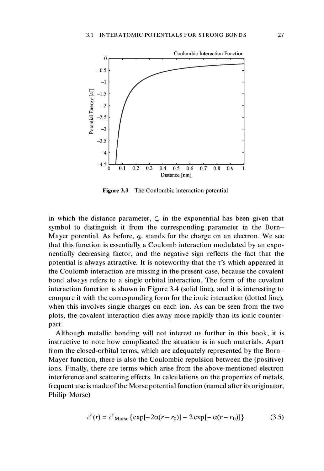
potential is shown in Figure 3.3.
Unlike the interactions described in the preceding two paragraphs, the
covalent interaction is never repulsive. And whereas the preceding functional
forms dealt with in this section can be shown to be exact solutions of the
corresponding situations, the functional form that best describes the covalent
interaction potential should really be regarded as being empirical. It is
C.4)

3.1 INTERATOMIC POTENTIALS FOR STRONG BONDS
27
Coulombic Interaction Function
a?
-4.5
0 0.1 0.2 0.3 0.4 0.5 0.6 0.7 0.8 0.9 1
Distance fnm]
Figure 3.3 The Coulombic interaction potential
in which the distance parameter, £, in the exponential has been given that
symbol to distinguish it from the corresponding parameter in the Born-
Mayer potential. As before, qe stands for the charge on an electron. We see
that this function is essentially a Coulomb interaction modulated by an expo-
exponentially decreasing factor, and the negative sign reflects the fact that the
potential is always attractive. It is noteworthy that the x's which appeared in
the Coulomb interaction are missing in the present case, because the covalent
bond always refers to a single orbital interaction. The form of the covalent
interaction function is shown in Figure 3.4 (solid line), and it is interesting to
compare it with the corresponding form for the ionic interaction (dotted line),
when this involves single charges on each ion. As can be seen from the two
plots, the covalent interaction dies away more rapidly than its ionic counter-
counterpart.
Although metallic bonding will not interest us further in this book, it is
instructive to note how complicated the situation is in such materials. Apart
from the closed-orbital terms, which are adequately represented by the Born-
Mayer function, there is also the Coulombic repulsion between the (positive)
ions. Finally, there are terms which arise from the above-mentioned electron
interference and scattering effects. In calculations on the properties of metals,
frequent use is made of the Morse potential function (named after its originator,
Philip Morse)
orSe{exp[-2a(r- r0)] - 2exp[- a(r- r0)]}
C.5)

28
ENERGIES, FORCES AND BONDS
Covalent Interaction Function
0.1 0.2 0.3 0.4 0.5 0.6 0.7 0.8
Distance [nmj
Figure 3.4 The covalent interaction function, with the Coulombic interaction indicated by
the dotted line
in which the parameter a is a distance factor not unlike those which appear in
the Born-Mayer and covalent functions, although in this case it is an inverse-
distance. There is a second distance parameter, namely ro, which does not have
a counterpart in those other potential functions. It appears because the Morse
potential has both repulsive and attractive terms, and the ro is the distance at
which the potential function has its minimum value. Finally, <^Morse is a
coefficient that determines the depth of the potential well. It is a useful exercise
to differentiate the Morse potential once with respect to r, so as to convince
oneself that the potential really does have its minimum value at ro. That is to
say
= 0
C.6)
r=r0
It is also interesting to note, in passing, that the Morse potential has the
useful feature that the exponent of the first term is precisely double that of the
second term. This makes for economy of computation, which is an important
consideration in large-scale calculations on metallic crystals. The form of the
Morse potential is indicated in Figure 3.5 which shows a minimum of- ^Morse
at the equilibrium separation.

3.2 INTERATOMIC POTENTIALS FOR WEAK BONDS
29
Morse Function
-0.06
0 0.1 0.2 0.3 0.4 0.5 0.6 0.7 0.8 0.9 1
Distance [nm]
Figure 3.5 The Morse function
3.2 Interatomic Potentials for Weak Bonds
Having covered the various forms of strong interaction, we turn now to
the weaker bonds, and begin with the attraction that can occur between
filled orbitals. That there should be repulsion when filled orbitals approach
sufficiently closely is not surprising, because the Pauli Exclusion Principle will
ultimately prohibit overlap of the orbitals belonging to the two atoms. As we
saw earlier, this provided the basis for the work of Born and Mayer. That there
should also be an attraction, as the distance increases beyond the equilibrium
separation, is more surprising. As was first demonstrated by Johannes van der
Waals, the interaction arises from the instantaneous dipoles that nevertheless
exist even in completely filled orbitals (see Chapter 2). Van der Waals was able
to show that this interaction varies as the sixth power of the distance, so we have
C.7)
in which P is a coefficient.
The two factors, repulsion and attraction, both appear in the Buckingham
potential function (named for R.A. Buckingham). It has the form
(r)= Aexp(-r/p)-p/r6
C.8)

30 ENERGIES, FORCES AND BONDS
We see that this is nothing other than a composite of Born-Mayer and van der
Waals terms. Although the Buckingham function is precise with respect to both
the repulsive and the attractive terms, it is not particularly suited to computer
simulations, because it comprises a mixture of exponential and power expres-
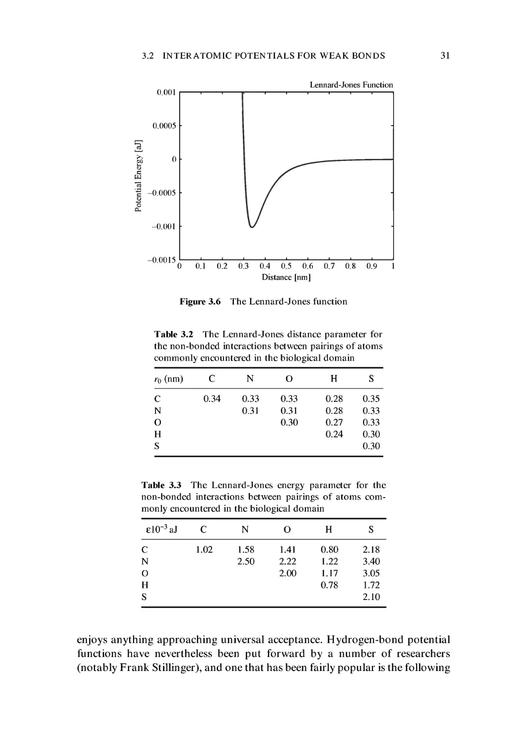
expressions. In this respect a potential developed by John Lennard-Jones is much
easier to deal with. This function has the form
^(r) = £ {(r0 /rI2 - 2(r0 /rf } C.9)
There are just two parameters, namely the distance parameter r0 and an energy
parameter e. As was the case with the Morse potential, we see that the repulsive
term is simply the square of the attractive term, though in this case one is
dealing with powers rather than exponentials. This simplifying factor has made
the Lennard-Jones potential function extremely popular in the computer simu-
simulation of all manner of atomic and molecular systems, and it has become the
standard choice when the so-called non-bonding interactions must be included
in a calculation. The reader should be warned that the Lennard-Jones function
is sometimes written in the alternative form:
^(r) = £{(ro/rI2-(ro/rN} C.10)
This lacks the coefficient 2 in the second (attractive) term. The advantage of the
former version is that it admits of very simple interpretations for the two
parameters, namely that the energy minimum occurs at a distance r0, and that
the depth of the potential well is simply -£ (see Figure 3.6). The reader may find
it instructive to check these facts by, as before, taking the first derivative of the
potential with respect to r and equating this to zero. That is to say
=0 C.11)
1-го
The reader should also make careful note of the fact that the interatomic
potential, by convention, always goes to zero as r tends to infinity. That is to say
<fi>)Loo= 0 C.12)
Tables 3.2 and 3.3 list the values of r0 and £, respectively, for non-bonded
pairings of atoms of various elements.
Finally, amongst the purely central forces, there is the hydrogen bond (see
Chapter 2). This has been the subject of a great amount of discussion in the
literature, and it has not proved possible to derive a functional form which

3.2 INTERATOMIC POTENTIALS FOR WEAK BONDS
31
0.001
0.0005
о
-0.0005
-0.001
n nm <ч
Lennard-Jones Function
■
0 0.1 0.2 0.3
0.4 0.5 0.6
Distance [nm]
0.7 0.8 0.9 1
Figure 3.6 The Lennard-Jones function
Table 3.2 The Lennard-Jones distance parameter for
the non-bonded interactions between pairings of atoms
commonly encountered in the biological domain
r0 (nm)
N
О
H
0.34
0.33
0.31
0.33
0.31
0.30
0.28
0.28
0.27
0.24
0.35
0.33
0.33
0.30
0.30
Table 3.3 The Lennard-Jones energy parameter for the
non-bonded interactions between pairings of atoms com-
commonly encountered in the biological domain
£l(T3 aJ С
N
О
H
1.02
1.58
2.50
1.41
2.22
2.00
0.80
1.22
1.17
0.78
2.18
3.40
3.05
1.72
2.10
enjoys anything approaching universal acceptance. Hydrogen-bond potential
functions have nevertheless been put forward by a number of researchers
(notably Frank Stillinger), and one that has been fairly popular is the following

32 ENERGIES, FORCES AND BONDS
%? Wiomc(r)+ Ws(r) C.13)
in which (fLj(/) is the Lennard-Jones potential (with parameters chosen to
correspond to the non-bonding situation), Фюшс(г) is the Coulombic inter-
interaction given by Equation C.3), and (Ps(r) is known as a switching function. The
effect of the latter is to make the overall (p(r) go smoothly to zero for distances
greater than a critical value, which is usually taken to be 0.285 nm.
3.3 Non-central Forces
Let us now move on by taking a brief look at the complexities that arise when
one takes non-central components of the interatomic force into account. Faced
with such a task, one finds that progress can be made only if one adopts an
empirical approach, using approximations where necessary. A study along
these lines has produced an expression for the total energy of a molecule that
is now widely used in computer simulations of biological molecules. It has the
following form
C 2 [k2(b-b0J+ к3ф-Ь0K + к4ф-Ь0L]
b
J + *(ееK + *(е eL
(e" e°J + *з(е" е°K + *4(е~ e°L
C1 -cos(|))+ k20 ~ cos2(|))+ къ{\- cos3(|))
*2X2+ S
b,b'
k(b - bo)(Q -60)+
b,Q 6,ф
+ У (9 - Q0)[k i cos ф + k2 cos 2ф + k3 cos Зф]
еф
- GoKe' - Go) + У k(Q - Qo)(& - %) cos ф
C.14)
2(J/)9_3(J/N
Гц Г;;
Such a potential can be regarded as deriving from two types of interaction: the
valence terms and the non-bonded terms, the latter referring to those compon-
components that do not stem from covalent bonds. The valence terms themselves also
come from different categories of interaction, namely what are called the
diagonal components and the off-diagonal cross-coupling components. In the

3.4 BOND ENERGIES 33
valence terms, there are the internal coordinates of bond length, b, angle, 9,
torsion angle, ф, and out-of-plane angle, %. The cross-coupling terms include
the various possible combinations of two and three internal co-ordinates, and
they are found to be important if good agreement with experimental vibration
spectra is at a premium. This is generally the case, because large biological
molecules are not static at body temperature; their dynamic properties are of
great significance for metabolic function. The non-bonded terms include a
Lennard-Jones type function that has a ninth rather than a 12th power in its
repulsive part; the repulsion is thus somewhat softer than the case discussed
earlier in this chapter.
3.4 Bond Energies
Before putting interatomic potentials to use, it will be helpful to get an idea of
the energies of the bonds commonly encountered in molecules of biological
relevance. This will give us a better view of the types of reactions and processes
that can occur in the biological domain. We will be considering many cases in
which molecules are subjected to one influence or another, and it is important
that we develop a feeling for what might happen under a given set of circum-
circumstances. We might wish to know whether a given molecule is likely to be able to
withstand certain conditions. Why is it, for example, that sitting in the sun can
cause a change in the colour of the skin, whereas the same is not the case when
we sit in front of a fire, even though the latter may be just as effective at giving
us instant warmth?
A few calculations relevant to our own bodies will serve to illustrate the
usefulness of being able to make quantitative estimates. It can readily be shown
that the total energy of all the bonds in a typical adult body is about 250 times
the energy we consume in a single day. Let us make the following approxima-
approximations. First, we assume that the bonds which keep our bodies together are
essentially of the С—С type. This is not true, of course, because there are many
C-N and С—О bonds, but we will later discover that these two types of bond
have rather similar energies anyway. Now there are roughly 5 x 1022 atoms per
gram of tissue, and we can assume that there would be about three bonds per
atom (i.e. that the degree of bonding is slightly larger than would be the case if
all bonds occurred only in linear chains, with their two bonds per atom). This
indicates that an adult human would comprise about 4 x 1027 bonds. A typical
covalent bond energy is approximately 0.6 aJ (i.e. 0.6 x 10~18J), so the total
energy of all the bonds in the body is about 2.4 x 109 J or 0.6 x 109 calories,
which is indeed about 250 times the normal daily intake of 2400 kilocalories, in
the well-fed portion of the world's population at least.
Table 3.4 shows the characteristics of a number of interatomic bonds of
biological relevance. It is particularly those that involve a single bond that will

34 ENERGIES, FORCES AND BONDS
Table 3.4 The interatomic bond energies and interatomic
equilibrium separations for a number of pairings and bond
types encountered in biological molecules
Bond
H-H
H-C
H-N
H-0
C-C
C=C
C=C
C-N
C=N
C=N
C-0
c=o
N-N
N=N
N=N
N-0
N=O
0-0
0=0
Energy (aJ)
0.72
0.69
0.65
0.77
0.58
L.02
1.39
0.49
1.02
L.48
0.58
1.23
0.26
0.69
L.57
0.35
0.80
0.35
0.82
Distance (nm)
0.074
0.109
0.100
0.096
0.154
0.135
0.121
0.147
0.129
0.115
0.143
0.122
0.148
0.124
0.100
0.144
0.120
0.149
0.128
be of importance, although it is instructive to compare these with the situations
in which two, or even three, bonds are involved. It must be emphasized that all
the bonds shown in Table 3.4 are of the covalent type. This means that the
equilibrium interatomic separation, shown in the final column of the table,
would arise from a balance between Born-Mayer repulsion and covalent
attraction.
We are now in a position to calculate the total energy represented by the
bonds in a simple molecule, assuming that its structure is already known. All
we have to do is to work out how many bonds of each type there are and then
look up the energies of these bonds in Table 3.4. It is true that we will then be
ignoring the non-bonding terms, but this is a reasonable approximation for
small molecules, in which remote parts of the molecule are not able to ap-
approach one another, as it adopts its three-dimensional conformation. Such
close approaches would give extra contributions to the energy. A good example
of a molecule in which the non-bonding terms are relatively small is glucose,
shown in Figure 3.7. Just below that figure, a table is given which shows the
small bookkeeping exercise that underlies the calculation of the total energy of
all the bonds in the molecule, namely 15.64 aJ.
Glucose is the molecule that is broken down in the mitochondria (singular,
mitochondrion) of every cell, during the respiration process. The final product

3.4 BOND ENERGIES
35
H2COH
H OH
Number Type
C-C
C-0
C-H
O-H
Energy
(aJ)
2.90
4.06
4.83
3.85
Total
15.64
Figure 3.7 The energy stored in all the bonds present in a glucose molecule
is water and carbon dioxide, together with the liberated energy. Using an
approach similar to the one we have just employed in connection with the
total binding energy of the glucose molecule, we can derive the following
equation for the respiration process
C6Hi2O6
-15.64aJ
6O2
-4.92aJ
6CO2
- 14.76 aJ
6H2O
-9.24aJ
3.44 aJ C.15)
in which the total bond energy in each component is shown underneath.
In reality, the mitochondria produce only about 2 aJ of useful energy from
each glucose molecule that is broken down, so the efficiency of this process is
just over 50%. It ought to be noted, however, that very few industrial processes
approach this level. It should also be noted that this simple calculation has
ignored non-covalent interactions. A more exhaustive calculation would have
taken both primary and secondary interactions into account. In the next
chapter, we are going to discover that calculations involving only bond energies
are, in any event, inadequate; one really needs to work with what is known as
the free energy, which includes, in addition to the energy term, one that
accounts for the entropy changes occurring during the reaction. These prin-
principles will be illustrated when we consider the physics of protein structure. The
reason the weak, non-bonding interactions are important stems primarily from
their large number. In principle, each atom in a molecule has this type of weak
interaction with all those atoms it is not covalently bonded to, and that number
will invariably be much larger than the number of covalent bonds. This fact is
illustrated in the following example.

36
ENERGIES, FORCES AND BONDS
The well-known polymer polyisoprene occurs with two different arrange-
arrangements of its side-chains. These are known as the cis- and £rans-isomers. They
are commonly known as natural rubber and gutta-percha, respectively. The
noteworthy thing is that whereas natural rubber is very flexible, gutta-percha is
stiff and hard. (Interestingly, both these isomers were used in the golf balls of
earlier decades, the natural rubber providing the elastic core and the gutta-
percha being used for the stiffer outer cover.)
Because these two polymers have the same backbone structure, and also
the same side groups, the difference in their mechanical behaviour must
derive solely from the non-bonded interactions. In the cis configuration (see
Figure 3.8), the methyl group (i.e. the CH3 group) interacts with the hydrogen
atom on the same side of the double bond's axis, this interaction preventing the
methyl group and the hydrogen atom from rotating away from each other. As a
result, the chain develops a kink, the methyl and the hydrogen repelling each
other until equilibrium prevails. The kink in the backbone can be straightened
out by the application of sufficient tensile stress, but as soon as this stress is
released the repulsive forces between the two side groups in question cause the
kink to develop again in the same place. In the trans configuration (see Figure
3.9), the methyl group and the hydrogen are located on opposite sides of the
double bond's axis, so the backbone does not develop kinks. It is for this reason
Figure 3.8 The naturally kinked molecular configuration of ds-polyisoprene gives it a
high degree of elasticity
Figure 3.9 Molecules of ?rans-polyisoprene do not have the kinked structure of their cis
counterparts and they are far more rigid

3.4 BOND ENERGIES
37
that gutta-percha does not show the same elastic effects. It is true, of course, that
gutta-percha is not ideally stiff; with the application of sufficient tensile stress, it
can be extended, but this requires elongation of the covalent bonds, and that
requires a far greater force. The same is true of the cis form, which can be further
extended after the normal elastic extension has been reached, but again the
further extension requires application of much greater force.
As we have just seen, the cis and trans forms of polyisoprene differ with respect
to rotation about a double bond. The resistance to such rotation is known as
steric hindrance, and it has actually been measured for some simple polymers.
For polyethylene, for example, the variation of energy as a function of the angle
of rotation about the double bond was found to be as shown in Figure 3.10, in
which the trans form is defined as having zero rotation angle, while the cis form
corresponds to an angle of 180°. The inset to the figure shows the situations
viewed parallel to the backbone, and it is clear that the cis form will give rise to
larger non-bonded energy contributions, because of the close proximity between
the various hydrogen atoms. It is interesting to note, both from the experimental
curve and also from the inset, that the 120° case also corresponds to a local
minimum of non-bonded interaction energy called the gauche form.
As an exercise in the application of potential energy functions, one can
attempt to justify the general form of Figure 3.10 by directly computing the
various non-bonded energy contributions. As can be seen in Figure 3.10 (inset)
Trans
0.03 -
Peak
Gauche
О 20 40 60 80 100 120 140 160 180
Rotation Angle
Y
H H
Trans
Gauche
HH HH
Cis
Figure 3.10 The experimental rotational energy function for twisting about one of the
C-C bonds in polyethylene

38
ENERGIES, FORCES AND BONDS
there are four hydrogen atoms to be taken into account, these occurring in two
pairs. Within either pair, the mutual positions of the hydrogen atoms do not
vary, so one needs to take into consideration only those energy contributions
that arise from the inter-pair interactions. One needs to know the precise
geometry of the situation, in order to first calculate the relevant distances
and then compute the corresponding energies. Each carbon atom can be
imagined as being positioned at the centre of a tetrahedron, as far as the mutual
angles of the corresponding bonds are concerned. On the other hand, the
various atoms with which it shares covalent bonds will not in general lie at
the corners of a rhombohedron, because the distances involved are not all
the same. This is made clear in Table 3.4, in which we see that the С—H bonds
are 0.109nm long, whereas the С—С bond has a length of 0.154nm. One
can assume that the non-bonding interactions are adequately described by a
Lennard-Jones potential function of the type
r) = e{(ro/r)n-2(ro/rN}
C.16)
withe = 3 x 10aJ.
It is important to note that these energy and distance values differ consider-
considerably from those listed for the H—H bond in Table 3.4. The reason for the
difference lies in the fact that those table entries are for covalent bonds,
whereas we are here dealing with the much weaker non-bonded interaction.
Although the geometry is not particularly easy, one can work out the distances
of the various non-bonded interactions, and the corresponding energies. The
results of this book-keeping exercise are shown in Figure 3.11 for the trans,
Trans
0.03 -
Peak
Gauche
0 20 40 60 80 100 120 140 160 180
Rotation Angle
Figure 3.11 The calculated rotational energy function for twisting about one of the C-C
bonds in polyethylene using Tables 3.2 and 3.3

3.5 SPRING CONSTANTS 39
peak, gauche and cis configurations, and the resulting energy values permit one
to draw an approximate curve. Although the values of the different points are
considerably lower than the corresponding points on Figure 3.10, the curve
does at least have the right general shape, with the cis form having the highest
energy, and the next highest value corresponding to what has been labelled
peak. The reason all the calculated energies are lower than the experimental
values lies in the fact that we have been neglecting the influence of the configur-
configuration changes on the underlying molecular orbitals, and perturbation of these
would lead to increases of energy. However, as mentioned earlier, this small
computational exercise has limited value in any case, because one should really
be working with the free energy rather than merely the potential energy. It is
thus appropriate that we suspend further discussion until we have considered
those aspects of thermodynamics and statistical mechanics that are relevant to
molecules and situations of biological interest.
3.5 Spring Constants
Until now in this chapter, we have been considering the forces that act at
the atomic and molecular level. In many biophysical problems, however, we
need to know something about the forces that act on a more macroscopic
level. These forces are ultimately due to those atomic and molecular level
forces, of course, but we need to be able to approximate the interactions that
occur at the grosser level, without having to think about their microscopic
roots.
These were the issues that occupied materials scientists of earlier centuries, in
fact, and they made commendable progress despite the primitive nature of
science in those days. One of the early giants in this type of endeavour was
Robert Hooke, who established that there is a linear relationship between the
stress applied to a piece of material and the resulting strain. This wisdom is
embodied in what came to be known as Hooke's Law, and he showed that the
simple proportionality holds as long as the degree of strain is small. As will be
discussed more fully in Chapter 5, it breaks down when the material is strained
beyond what is known as the elastic limit. The science of those early days
tended to be written up in Latin, and Hooke's result is immortalized in the
phrase ut tensio sic vis (the elongation is as the force).
When dealing with such multi-atom structures as the components of muscle
fibres, for example, it is customary to invoke Hookian behaviour, and to assume
that the macroscopic restoring force is linearly related to the strain, by an
expression of the type
^restoring — "" kAx C.17)

40 ENERGIES, FORCES AND BONDS
the negative sign arising because the force acts in the direction counter to the
extension Ax. The coefficient к is known as a spring constant, and we will
encounter examples in Chapters 5, 6 and 10.
Systems obeying Equation C.17) are said to be harmonic. If (following one of
Isaac Newton's laws) one replaces the force on the left-hand side with its
equivalent, namely mass times acceleration, and then solves the resulting differ-
differential equation, one obtains a solution that describes simple harmonic motion.
The classic example is, of course, the harmonic motion of a simple pendulum.
We should note also that Equation C.17) can be used in conjunction with
Equation C.1) to produce the (macroscopic) potential energy function that
underlies Equation C.17). We then find by integration that the potential energy
varies as the square of the displacement.
When the amplitude of a pendulum is large, the harmonic approximation
breaks down, and analysis of the motion then requires the use of elliptic
integrals. A fascinating finding of such analysis is that under certain conditions
the simple periodic solution is replaced by one describing a solitary wave. The
latter is now referred to as a soliton, in fact, and there have been suggestions
that such a mode of motion could be important to the dynamics of an enzyme.
Exercises
3.1 Many artificial joints now include metallic parts. The interactions between the
atoms in these components are well described by the Morse function
Ф(г) = CMorse{exp[-2a(r - r0)] - 2exp[-a(r - r0)]}
where typical values of the three parameters are Фмоке = 0.056 x 10~18 J,
a = 1.4 x lO^m and r0 = 2.8 xlO"lom. What is the maximum tensile force
that a pair of such interacting atoms can withstand, without being torn apart?
3.2 Two atoms in a biological molecule are found to interact in a manner that can be
described by the Lennard-Jones potential
^(r) = e{(ro/rI2- 2(ro/rN}
in which the parameters e and tq are constants. It is found that e = 0.49 x 10~18 J,
and that the minimum force required to totally separate the atoms is
8.96 x 10"9 Jm. At what separation distance would the two atoms be in mutual
equilibrium?
3.3 During a simulation of a multi-atom molecule, an analytical function was needed
to represent the interactions between the various pairs of atoms. There was the
requirement that the chosen function should have the correct value of the mini-
minimum energy, фтт, and that this should lie at the correct atomic separation

3.5 SPRING CONSTANTS 41
distance, r^m.n. Moreover, the atomic separation distance corresponding to the
maximum attractive force also had to be the specific value ry-max.
The initial choice was the Lennard-Jones function, and this was reasonably
successful because a proper fit to all three of the above-named numbers was
possible. But the shape of the Lennard-Jones function was not quite suitable, so it
was decided to try the Morse function instead. The hope was that the larger
number of parameters in the Morse function (three, compared with the Lennard-
Jones function's two) would lead to a more suitable shape. The question then
arose, however, as to whether it would still be possible to fit the function to those
above-mentioned three numbers.
After analysing the situations corresponding to the two different potential
functions, do you believe that the second fit would have been possible, and if
so, under what conditions?
3.4 The recently-developed technique known as 'optical tweezers' permits measure-
measurement of the forces applied to single biological molecules. Calculate the maximum
tensile force that a polypeptide chain can withstand, assuming that the covalent
bonds which hold the backbone together can be described by the Lennard-Jones
potential function:
^(r) = e{(ro/rI2-2(ro/rN}
in which the values of e and r0 for carbon-carbon bonds are respectively
0.56 x 10~18J and 0.152 x 10"9m, while the corresponding values for carbon-
nitrogen bonds are respectively 0.51 x 10~18 J and 0.149 x lO^m.
Further Reading
Atkins, P. W., A990). Physical Chemistry. Oxford University Press, Oxford.
Baker, J. J. W. and Allen, G. E., A974). Matter, Energy andLife. Addison-Wesley, Reading,
MA.
Barua, A. K., (L959). Force parameters for some nonpolar molecules on the exponential 6-8
model. Journal of Chemical Physics 31, 957-960.
Berendsen, H. J. C. et al., A981). Interaction models for water in relation to protein
hydration. In B. Pullman (Ed.) Intermolecular Forces. Reidel, Dordrecht, pp 331-342.
Born, M. and Mayer, J. E., A932). Zur Gittertheorie der Ionenkristalle. Zeitschrift fur
Physik 75, 1-18.
Buckingham, R. A., A938). The classical equation of state of gaseous helium, neon and
argon. Proceedings of the Royal Society (London) A168, 264-283.
Hirschfelder, J. O., Curtiss, C. F. and Bird, R. В., A954). Molecular Theory of Gases and
Liquids. John Wiley and Sons, New York.
Janzen, A. and Leech, J. W., A976). Elastic constants of the inert gas solids. Canadian
Journal of Physics 54, 227-238.
Keener, J. and Sneyd, J., A998). Mathematical Physiology. Springer-Verlag, Berlin.
Lennard-Jones, J. E., A924). The determination of molecular fields from the equation of
state of a gas. Proceedings of the Royal Society (London) A106, 463^77.
Lennard-Jones, J. E., A931). Cohesion. Proceedings of the Physical Society (London), A43,
461^82.

42 ENERGIES, FORCES AND BONDS
Margenau, H. and Kestner, N. R., A969). Theory of Intermolecular Forces. Pergamon,
Oxford.
Mason, E. A. and Rice, W. E., A954). The intermolecular potentials for some simple
nonpolar molecules. Journal of Chemical Physics 22, 843-851.
Morse, P. M., A929). Diatomic molecules according to the wave mechanics II Vibrational
levels. Physical Review 34, 57-64.
Moore, W. J., A972). Physical Chemistry. Longman, Englewood Cliffs, NJ.
Murray, J. D., A989). Mathematical Biology. Springer-Verlag, Berlin.
No, K. T. et al., A995). Determination of non-bonded potential parameters for peptides.
Journal of Physical Chemistry 99, 13019-13028.
Pauling, L., A960). The Nature of the Chemical Bond Cornell University Press, Ithaca, NY.
Pauling, L., A970). General Chemistry Freeman, San Francisco.
Price, S. L., A996). Applications of realistic electrostatic modelling to molecules in com-
complexes, solids and proteins. Journal of the Chemical Society, Faraday Transactions 92A7),
2997-3008.
Salviucci, P., ed., A967). Molecular Forces North-Holland, Amsterdam.
Sun, H., A998). COMPASS: an ab initio force-field optimized for condensed-phase appli-
applications - overview with details on alkane and benzene compounds. Journal of Physical
Chemistry В 102, 7338-7364.

Rates of Reaction
The discussion in the two preceding chapters was strictly applicable to a state
that is not actually attainable, namely the absolute zero of temperature, for it
ignored the thermal motions that all atoms and molecules must have when they
are at a finite temperature. And when considering the motions of atoms and
molecules in biological matter, it is never permissible to regard the individual
entities as moving completely freely, as they are imagined to do in an ideal gas.
Cooperative effects are much in evidence, and this invariably makes the situ-
situation complicated. Understanding the collective properties of interacting
groups of atoms and molecules was a challenge that occupied theoretical
physicists and chemists in the late 19th century, and despite much progress,
the situation remains less than perfect even to this day. At the turn of the
millennium, there was still no universally accepted theory of the liquid state.
Indeed, Philip Anderson expressed the opinion that understanding the glass-
liquid transition had become the most pressing issue in all of condensed-matter
science.
In the present chapter, we will see that the energies invoked in the previous
two chapters must be replaced by free energies. And we will then go on to
consider the factors that dictate the most probable forms of molecules, under
given thermal conditions.
4.1 Free Energy
When one is concerned with changes in the state of a system, a full description
of the situation requires knowledge of what is known as the free energy. There
are actually two different forms of free energy, one first proposed by Helmholtz
and the other by Gibbs.
The Helmholtz free energy, F (named for Hermann von Helmholtz), is a
function of the internal energy, (pint, the absolute temperature, T, and the
entropy, S (see Appendix C). The relationship is
F=%nt-TS D.1)

44 RATES OF REACTION
The Gibbs free energy, G (named for Josiah Willard Gibbs), includes an
additional term that depends upon both the pressure and the volume. This
more inclusive form of the free energy is described by the following equation
G=^int + PV -TS D.2)
We will discuss the nature of the internal energy shortly. The general rule is
that a system can spontaneously alter its status if the change results in a
lowering of the free energy. And as a corollary of this, a system will be in
equilibrium if its free energy is at a minimum. Possible changes in a system can
thus be anticipated if one has a complete knowledge of all the components of
the relevant free energy, as a function of the independent variables. Given the
functional forms of these components, one can differentiate with respect to the
relevant variables, to see whether equilibrium prevails or whether spontaneous
changes in the system can be expected. If the changes are to occur under
constant temperature and volume, it is usually adequate to work in terms of
the Helmholtz free energy. But the reactions that occur in the body usually take
place at constant pressure, so it is more common to work through the Gibbs
free energy.
An important feature of both forms of free energy is the final term, and its
negative multiplier. When the temperature is very low, this term will be insig-
insignificant of course, but with increasing temperature it makes its influence felt,
the degree of this depending upon the entropy. Unlike the other terms in these
free energy expressions, entropy is still an incompletely-understood concept.
That fact too will be discussed later in this section (as well as in Appendix C).
Suffice it to say that the final term in either of the free energy expressions will
have a greater influence if the entropy is greater.
Returning to the internal energy, the first thing to be noted is that this would
consist entirely of kinetic energy if there were no interactions between the
particles in a system. As we saw in the preceding chapter, when considering
interatomic potentials, these interactions certainly do exist, and many can be
described by reasonably simple functions. Those interatomic potentials were all
defined in such a way that the interaction energy became zero at very large
distances. This is mathematically reasonable, of course, but we should not
confuse very large separations with equilibrium conditions. On the contrary,
two atoms will attract one another even if the distance between them is quite
large, although the force of attraction will admittedly be very small indeed. For
our purposes here, the minimum in the interaction potential is more relevant.
This does represent a position of equilibrium. When calculating the internal
energy, the potential energy component is indeed referred to this equilibrium
situation. In other words, thermodynamic potential energies are calculated
relative to the minimum in the potential well. Internal energy is defined by the
following equation

4.2 INTERNAL ENERGY 45
Cg? Cgr Cg?
<Pinl = ^pot + 0kin D.3)
in which (ppot is the potential energy, and (r^in is the kinetic energy.
4.2 Internal Energy
To see how the various components in the internal energy arise, let us begin by
considering a system of just two atoms. When they are at their equilibrium
separation, and stationary, there is neither potential nor kinetic energy, so the
internal energy is simply zero. If we now disturb the system by increasing the
interatomic separation, by a few per cent say, the system will acquire potential
energy. If the atoms are then released, they are free to move and they will
approach each other with increasing velocity, ultimately passing the equilib-
equilibrium separation and then overshooting this, so that the separation is now less
than the equilibrium distance. As the equilibrium point is passed, the potential
energy will be momentarily zero, but the kinetic energy will be finite (and at its
maximum value for the given starting conditions). The initial potential energy
of the displacement will thus have been fully converted into kinetic energy.
Ultimately, when the overshoot is such that the potential energy has again
reached the value it had when the atoms were released, the kinetic energy will
once more have become zero. The direction of motion will then be reversed,
and the interatomic separation will again start to increase. As it passes the
equilibrium separation, there will again be zero potential energy but finite (and
maximum) kinetic energy. If the system is not further disturbed, these oscilla-
oscillations will continue indefinitely, the mutually staggered situations of (r>pot = 0
and (pkin = 0 regularly alternating. In between these extremes, both potential
energy and kinetic energy will of course be finite.
As can readily be imagined, the situation becomes far more complicated if the
number of atoms is increased, and it is then best handled statistically. In an
arbitrarily disturbed system, it will be highly unlikely that all atoms simultan-
simultaneously have zero kinetic energy, and in any event the zero potential energy
situation cannot prevail unless the number of participating atoms is very small.
This is not to say that equilibrium cannot be attained, however, because a
balance between repulsive and attractive forces can still be achieved even though
some of the interatomic spacings differ from the equilibrium two-body value.
As we have just seen, the kinetic energy arises from the motions of the
individual atoms, and the formal definition of this parameter for a system
comprising N atoms is simply
£v? D.4,
1=1

46 RATES OF REACTION
where vt is the speed (not velocity) of the rth atom. As is shown in Appendix C,
and assuming that what are known as Maxwell-Boltzmann statistics (named
for James Clerk Maxwell and Ludwig Boltzmann) apply, there is a relatively
simple relationship between these atomic velocities and the temperature. If the
system is a three-dimensional one, which is to say that the positions of all the
atoms require three different variables to describe them completely, the rela-
relationship between the velocities and the temperature is as given by the following
equation
kin = I 2 \NkBT D.5)
in which к в is the Boltzmann constant. The latter has the value 1.38054
xlO3 JK -1. Because the above equation does not take quantum effects into
account, it is said to define temperature in the classical limit. The factor 3/2 in
the final expression in this equation deserves some comment. Because the
system is three-dimensional, we see that each degree of freedom has квТ/2 of
energy associated with it. When a situation of equipartition prevails, there will
be equality between the potential energy and the kinetic energy. However, this
can be the case only if the particles interact through a strictly harmonic
potential (that is to say that the inter-particle interaction varies as the square
of the separation distance).
4.3 Thermodynamics and Statistical Mechanics
In our initial example of just two atoms, the kinetic energy and the potential
energy showed wild (and counter-phase) fluctuations between their maximum
and zero values. As mentioned earlier, with increasing numbers of atoms in the
system, these fluctuations would become less and less pronounced, because
the individual motions would not be likely to be all in phase with one another.
The system is then best described statistically, and for a sufficiently large
number of particles, the temperature, for example, will not fluctuate to any
appreciable degree. One of the conceptual difficulties encountered by those who
study biological molecules is related to the limited number of atoms in such an
entity. It might then appear to be the case that fluctuations in potential energy
and kinetic energy really do occur. This ignores the fact that a biological
molecule is not normally an isolated system, unless it happens to be floating
freely in a vacuum (as in interstellar space, for example). Even then, energy can
be received from and emitted to the surroundings, in the form of radiation. In
general, the molecule will be in thermal contact with its surroundings, which
might consist of other molecules, or water, or indeed a combination of both.

4.3 THERMODYNAMICS AND STATISTICAL MECHANICS 47
The product PV defines the external energy, and the sum of the internal and
external energies is known as the enthalpy, H, which is thus defined by the
equation
H = <Snt + ^ext = Koi + ?kin + PV D.6)
One thus sees that the Gibbs free energy is obtained simply by replacing the
internal energy in the Helmholz free energy by the enthalpy.
Now let us turn to the more difficult issue of entropy. This can be approached
in two different ways, one being that due to Boltzmann, who was the first to
appreciate its existence. Right from the outset let us correct a very widespread
misconception regarding this elusive parameter. It is a mistake simply to equate
entropy to the degree of spatial disorder in a system. On the contrary, as has
become appreciated in recent years, the ordered and disordered states of a
system, at the same density and temperature, can actually have essentially the
same entropy (see Appendix C). The popular misconception regarding entropy
arises from a failure to distinguish between the mere configuration of a system
and its distribution of possible states, the latter including the states of motion.
When Boltzmann carried out his pioneering studies on the subject, it was the
latter attribute that he focused on.
One could say that concentrating solely on the instantaneous configuration
of a system ignores the way in which this influences the motions of the
individual atoms. The point is that the individual atoms are not simply free
to move as they please. On the contrary, their motions will be constrained by
the instantaneous atomic configuration of the entire assembly. In other words,
entropy is determined by the fundamental cooperativity in the system, and
probing this can be a very complicated matter indeed. That this is true is
attested to by the fact that we still do not have a completely satisfactory
description of the liquid state (see Appendix C). There are theories that treat
liquids as if they were disordered solids, and there are other theories which look
upon a liquid as a condensed gas. Neither of these approaches is really satis-
satisfactory, and there is now a growing appreciation of the fact that the liquid state
is fundamentally different from either of those other two extremes (except
above the critical point, of course).
Boltzmann's statistical treatment of entropy defined this by the relationship
S=kB\nQ. D.7)
in which Q is related to the probability of a state, as measured by the number of
ways in which it can be realized. It is important to appreciate the fact that the
word state involves both the positions and the velocities of all the atoms in the
system; as noted above, one cannot draw conclusions regarding the entropy
merely from consideration of the instantaneous atomic arrangement.

48 RATES OF REACTION
The states referred to in the above definition of entropy occur in what is
know as phase space, rather than simple configuration space, the difference
being that phase space includes dimensions for velocity as well as position. The
nature of entropy can be appreciated by considering various extreme cases,
one of which was our two-atom system discussed earlier. It will be recalled that
the regular oscillations of this system caused the positions and velocities to
systematically sweep through a continuous set of values. However, there was a
relationship between position and speed that was always rigidly adhered to;
a given position always implied one given speed. In the other extreme of a
many-atom gas, a given set of positions for all the atoms could conceivably be
associated with many different instantaneous speeds of these particles, so the
system would explore a much larger region of phase space. If one compares the
situation in a crystal and in a glass, at the same density and the same low
temperature, the individual atoms perform oscillations in local potential-
energy wells that are approximate multi-dimensional parabolas, that is to say
hyper-parabolas (not to be confused with hyperbolas, of course).
The entropies of those two states may thus be quite similar. However, as the
temperature rises, there are co-operative effects in the crystal that force
the individual atoms to move coherently with respect to one another, these
motions being collectively described by the waves known as phonons. The
disorder in the glassy state prevents cooperativity occurring to the same extent,
and there is more randomness in the individual motions. With increasing
temperature it is this, rather than mere disorder in the atomic positions, which
gives the glass a higher entropy than the crystal, at the same density and
temperature.
The existence of entropy became clear in the nineteenth century, even before
it was confirmed that individual atoms actually exist. The need to invoke such
an entity arose from considerations of the efficiencies of machines, and the
pioneers of thermodynamics (particularly Lord Kelvin - born William Thom-
Thomson - Sadi Carnot and Rudolf Clausius) realised that the departure from ideal
efficiency is intimately linked to the existence of such a randomising factor.
Indeed, that branch of science worked with a different definition of entropy,
namely that
dS = dQ/T D.8)
where dS is the increment of entropy and dQ is the amount of heat energy
absorbedhy a system, in what is known as a reversible fashion. The point to be
made here is that if the heat absorbed by the system merely produces greater
incoherence between the atomic motions, this energy input will not be recover-
recoverable as useful work, and the entropy of the system will have increased.
This brings us to what is known as the First Law of Thermodynamics. It states
that if a system absorbs heat energy dQ, and if it has an amount of work dW

4.3 THERMODYNAMICS AND STATISTICAL MECHANICS
49
performed on it, the total increase in the internal energy will simply be the sum
of these two components. That is to say
int = dQ + dW = dQ -PdV/T
D.9)
where the last term in the second form of the equation applies if the work done
on the system is carried out at constant pressure. It is important to notice the
negative sign in the second form of this equation. We see a familiar example of
this fact every time we use a bicycle pump. Both the pump and the tyre become
warmer as more and more air is pumped into the tyre.
Having made a brief contact with thermodynamics, let us return to the
statistical nature of systems, which is the domain of that branch of science
known as statistical mechanics. We have already seen that we must think in
terms of phase space rather than simple configuration space, so the little
diagrams shown in Figure 4.1 are not quite as simple as they might at first
appear to be. They show a container that is divided into two parts by a barrier
that has a small hole in it. The left-hand diagram shows the rather unlikely
situation in which all the points representing the position and velocities of the
individual atoms, in an N-atom assembly, are in the same half of the container.
The right-hand picture, by contrast, shows a more probable situation in which
half of the points are in one part of the container and the other half are in the
other part. This is a combinatorial problem of the type that asks how many
different ways n items can be chosen from amongst a total of N items. The
difference is that in the present case these 'items' are actually states in phase
space. The principles are nevertheless the same, since we may interpret N as
being the number of elementary regions of phase space which can be occupied
at any one time by the states in the system. The number of ways, Q., in which the
Figure 4.1 These two different situations correspond to different degrees of filling the
available phase space

50 RATES OF REACTION
N items can be distributed in two groups comprising, respectively, n\ and n^
states is given by the simple combinatorial expression
TV!
Q=—I D.10)
where
N\=N(N -1)(N -2) ••• X2 xl D.11)
Irrespective of the initial state of the system, the passage of a sufficiently long
time will produce an equilibrium condition in which, apart from small fluctu-
fluctuations, there will be equally many molecules in the two halves of phase space, as
shown on the right-hand side of Figure 4.1.
It is a relatively simple matter to demonstrate that the right-hand side of the
above equation is greatest if щ and n2 are equal, whereas it continually
decreases as the difference between щ and ni increases. Because the most
probable situation will indeed correspond to approximate equality between
щ and «2, we see that the tendency is for the entropy of the system, that is to say
кв In Q., to increase. In other words, there will always be a tendency for the
states of a system to occupy as much of phase space as they are permitted.
Armed with this physical background, we can proceed to develop some
useful relationships between the various parameters. For a start, let us imagine
that a system of the above type is described by a set of states 1,2,3, ..., i, ...
which have corresponding energies 81,82,83, . ..,82, ... Furthermore, let the
number of elements in state 1 be йь in state 2 be ni, and so on. The total
number of elements will simply be
N = X m D.12)
Moreover, generalising what was stated earlier, the number of different ways in
which the N indistinguishable elements can be distributed is given by
TV!
Q DЛЗ)
Q Лiii
П\\ X Пг\ X Щ\ X • • • X Щ\ X • • •
We now wish to enquire as to which values of the different щ will give the
maximum entropy. Remembering that both 0! and 1! equal unity, the max-
maximum value of entropy will be obtained when all the щ equal unity or zero. The
entropy will then simply be кв In N!
Another relationship that follows automatically concerns the total energy,
<Ptotai- This is simply given by

4.3 THERMODYNAMICS AND STATISTICAL MECHANICS 51
«Kotal = X niEis DЛ4)
Moreover, as is shown in Appendix C, we obtain the interesting result that
щ = N x exp ( - Ei/kBT )/ E exP (- e,-АвГ ) D-[5)
i
and thus that the total energy is given by
<Ptotai =iV x У 8, exp (- 8г-/kBT )/ / exp (- Si/kBT ) D.16)
The denominator in the above two equations is a frequently occurring
quantity in statistical mechanics, and it has been given the name partition
function, which is usually denoted by the letter Z. That is
Z = J^Gxp(-Ei/kBT) D.17)
A formula that can be used to calculate the number of elements in the various
energy levels is known as the Boltzmann distribution. It gives the relationship
between those different elements (that is to say, states). Let us imagine that щ
and rij are the number of elements with energies ег and s,- respectively. Using the
above analysis, the desired proportionality is simply given by
^=ехр(-(8г-8;)АвГ D.18)
The Boltzmann distribution naturally applies only to systems that are in
thermal equilibrium.
It is useful to rewrite a number of the expressions that appeared earlier, using
the partition function. We thus have
S = Nk B In Z + NkBT(b In Z/ЬТ )V = NkB In Z + *$/T D.19)
because
^.§ D.20)
Z Ы
we get
F = -NkBT\nZ D.21)

52 RATES OF REACTION
One of the best-known applications of statistical mechanics is the derivation
of an expression which gives the probability of a particle being able to sur-
surmount an energy barrier of a given height. Indeed, it would be no exaggeration
to call this the classic example in this branch of science. Let us imagine that the
particle is in an energy well, and let its current energy be ф\. Furthermore, let
the top of the energy barrier correspond to the energy w-i- The height of the
energy barrier will therefore be Аф = ф2 — Ф\. We assume that the energy
varies continuously up the energy barrier, so that we can replace the discrete
summation normally found in the partition function with a continuous integral.
The probability that the particle has an energy in the interval [ф, Ф+ аФ\ is,
using an expression derived earlier,
/(ф)Aф = joo
Jo exp(-
Likewise the probability that the particle has an energy lying between ф\
and infinitely high energy is
Jo
exp
~
Jo exp (-^/квТ Щ
and similarly
f($> %2) = exp ( - Ург/квТ ) D.24)
We now note that of all the particles which have energy greater than ф\ а
fraction of them have an energy greater than the larger energy 02. This
fraction is simply given by
exp(- ф2/квТ) gs ,
—a? , =ехр(-АФ/квТ) D.25)
exp(- фх/квТ)
This is the desired result because it simply gives the probability that a particle
will be able to surmount the energy barrier. The right-hand side of this
equation is commonly referred to as the Boltzmann factor, and the reader
would be well advised to commit it to memory. Its chief consequences are
also worth remembering, namely that the probability of surmounting the
energy barrier increases as the height of the barrier decreases, and also as
the temperature increases.
As an example of the application of the entropy concept, we can use a
familiar little demonstration with a rubber band. The reader will find that the
demonstration is easier if a flat band is employed. As was noted earlier, in our

4.3 THERMODYNAMICS AND STATISTICAL MECHANICS 53
discussion of interatomic bonds, normal rubber is the name given to the
polymer ds-polyisoprene, in which the individual chains are kinked and inter-
interwoven in the relaxed form of the substance. There are numerous different ways
in which the disorder can be achieved, and they have associated with them a
relatively large volume of available phase space. This configuration of the
polymer chains is thus characterized by high entropy. If the rubber band is
stretched out to its full extent, all the polymer chains will lie roughly parallel to
one another and their kinks will have been removed. The access of the constitu-
constituent atoms to phase space will thereby be greatly reduced, and so the entropy
will fall.
If the stretching process is performed rapidly, so that no heat can flow out of
the system, the free energy will rise, and this will manifest itself through
increased heat content. The result will be a rising temperature, as can easily
be detected if the rubber band is pressed against one's moistened lips. If the
temperature of the band is now equilibrated with the lips, while maintained in
its fully-stretched condition, a subsequent release of the tension will cause the
opposite sequence to occur, and the band will suddenly feel cooler. (If the
reader performs this part of the experiment, care should be taken to avoid
pinching the lips as the band is released.)
In the second half of this little experiment, we have demonstrated that the
entropy rises again, and this causes a lowering of the free energy. A common
example of the use of the Boltzmann factor is encountered in the analysis of
particle diffusion in condensed matter. As we saw when considering the motions
of a pair of atoms, temperature manifests itself through atomic motion, and if
the atoms are constrained to move in a local potential energy well, these
motions will take the form of reasonably regular vibrations.
It will invariably be the case that there are escape routes from these energy
wells, the routes involving energy barriers of the type that were considered
above. A common problem thus arises as to what the escape rate will be, given
that the atomic vibration frequency is known. Since the probability of a
particle surmounting the energy barrier is simply given by the Boltzmann
factor, we can easily write an expression for the number of successful attempts
to surmount the barrier in a time t, given a vibration frequency of vatom- The
number of successful jumps, njumps, is simply given by
«jumps = vatom?exp (- Aif/kBT ) D.26)
where АЖ is the height of the energy barrier. This type of expression is
frequently encountered in analyses of atomic motions in crystals, and although
the energy barriers in biological molecules are not as well defined, the analysis
could certainly be extended to those cases as well. It should be noted, however,
that there are forms of condensed matter in which the energy-barrier concept
might not be particular useful. In a liquid, for example, although some analyses

54 RATES OF REACTION
have been couched in terms of similar energy barriers, there is evidence that this
is not what happens (see Appendix C). We touched on the issue earlier, when
noting that a liquid probably does not resemble a highly defective solid, as
some have conjectured.
We know the order of magnitude of several characteristic energies, so it
should be relatively straightforward to imagine how molecules are influenced
by various conditions. We earlier saw that the energy per degree of freedom is
given by ф=квТ/2. Because each particle will have six such degrees of
freedom, in a three-dimensional system, namely three for kinetic energy and
three for potential energy, the total energy per particle will be 3kвТ. Now the
temperature in the human body is about 310 K, so each atom will have energy
of the order of 10  aJ at its disposal.
Table 4.1 shows the latent heats of melting and evaporation for a number of
different substances, of various bonding classes. The transition energies natur-
naturally reflect the differences in the underlying interatomic interactions. Looking
at the entries in this table, and given the energy per atom which we have just
calculated, it is not surprising that some organic substances will melt when held
in the palm of one's hand. Conversely, one would not expect a hydrogen bond to
break at body temperature, even though the margin of safety is not all that
high. As can be seen from Figure 4.2, that margin is only about a factor of three
at body temperature. This is a serious consideration, given that the two strands
in each of our DNA molecules are held together by the hydrogen bonds that
bind the pyrimidine and purine portions in each base pair (see Chapter 7).
Different types of process in many-atom systems are naturally associated with
different characteristic energies. In general, the breaking of interatomic bonds
requires more energy than the mere redistribution of these. The stronger types
of bond obviously require more energy expenditure if they are to be ruptured.
Table 4.1 The transition energies naturally reflect the differences in the
underlying interatomic interactions
Argon
Chlorine
Germanium
Gold
Iron
Mercury
Sodium
Uranium
Water
Salt
Benzene
Element or
compound
(Ar)
(Cl)
(Ge)
(Au)
(Fe)
(Hg)
(Na)
(U)
(H2O)
(NaCl)
(C6H6)
Latent heat of
melting (aJ)
0.002
0.011
0.053
0.021
0.026
0.004
0.004
0.026
0.010
0.050
0.016
Latent heat of
evaporation (aJ)
0.011
0.034
0.557
0.541
0.585
0.099
0.L48
0.704
0.079
1.275
0.058

4.4 REACTION KINETICS
55
О—О ^Covalent = 0.6 aJ
О""О ^Hydrogen-bond = 0.03 aJ
О—
^Melting
= 0.002 aJ
Figure 4.2 Comparative energy levels
If the bond-breaking is to be accomplished thermally, the stronger bonds will
need warming to higher temperatures for a given rate of bond-breaking.
In fact, the situation is more complicated because many atoms can act co-
cooperatively to break a bond that would be beyond the disruptive capability of a
single moving atom. This is seen in enzymes, in which the energy of many
atoms is concentrated at a particular place. A fuller discussion of this import-
important process must be left until Chapter 7, however, when we discuss protein
structure. One might think that covalent bonds, which are much stronger than
hydrogen bonds, would not be vulnerable to breaking in this manner, but the
work of Alexander Fleming on bacteria suggested that this can indeed happen.
One day, when he was suffering from a cold, a few drops of nasal mucus fell
from his nose onto a culture of bacteria. Ever inquisitive, he decided not to
throw the culture away, and a few days later he was surprised to find that the
bacteria had been killed in the very area where the mucus had fallen. These
bacteria were protected by an outer shell, which comprised many covalent
bonds. Something in the mucus had apparently been capable of breaking
these bonds, and the enzyme in question is now known as lysozyme (the
structure of which was ultimately determined by David Phillips and his col-
colleagues). Later on, we will encounter enzymes that are similarly capable of
breaking the covalent bonds in the backbones of DNA molecules.
4.4 Reaction Kinetics
The rates at which chemical reactions proceed are governed by the principles
discussed above. However, in order to establish contact with what can be
observed experimentally, we need to discuss a number of formal definitions.
The reaction
A +
С
D.27)
is said to be mono-molecular, while the reverse reaction

56 RATES OF REACTION
С -» A + В D.28)
is said to be bi-molecular. The concentration of a given reactant has tradition-
traditionally been indicated by the relevant symbol contained within square brackets, so
the rate of consumption of species A in Equation D.27) is given by
while the rate of formation of species С is given by
f D.30)
It is also useful to define the reaction fluxes, J, and this introduces the
concept of the rate constant, customarily denoted by the letter k. If we write
A+B^+C D.31)
and
C^A+ В D.32)
we then have
Jc=k2[C] D.33)
and
JA=JB=ki№B] D.34)
It is worth noting that the rate constant is the inverse of a time constant, т.
The order of a reaction, n, is defined by
J = k[Cf D.35)
So we see that Equation D.33) describes a first-order reaction whereas the
reaction in Equation D.34) is second-order.
Let us now make contact with our thermodynamic foundations, and enquire
as to the influence of temperature on the reaction rate. A convenient starting
point is to define the chemical potential, which for a given component (sub-
(substance) i is given by

4.4 REACTION KINETICS 57
\Li= $ + RTlnOi D.36)
where/? is the gas constant (= 8.314 JK mol~l) and ix^ is the chemical poten-
potential of component / in the standard state. The chemical activity щ is related to
the concentration through the corresponding coefficient of activity, yt, by
at = yf[i] D.37)
These preliminaries completed, we can now consider the general reaction
\>AA + vBB ^ vcC + vDD D.38)
in which the V; are the stoichiometric coefficients, [f the changes take place
under constant pressure and constant temperature, and the changes are thus
limited to variations in the quantities of the reactants, the change in the Gibbs
free energy will be given by
AG = vC|Lic + vd\ld - VaMa - VbM-b С4-39)
Using Equation D.36), this can be rewritten as
AG = AG° + R T(vc In ac + vD In aD - vA In aA - vB In aB) D.40)
in which the changes have been referred to the molar standard reaction free
energy AG°, and where
AG° = vcVc + VdMd- Va\&- VbV°b D.41)
Gathering the logarithmic terms in Equation D.40), we obtain van't Hoff's
equation (first derived by Jacobus van't Hoff), namely
AG=AG°+*r Infect) D.42)
\aA aB J
If thermodynamic equilibrium prevails, the change in the Gibbs free energy
will be zero, and Equation D.42) can then be rewritten with the help of
Equation D.37) (putting all the coefficients of activity to unity, which is
justifiable if the concentrations are small). This produces an expression for
the important quantity known as the equilibrium constant, Keq, namely
D-43)

58 RATES OF REACTION
The final step in this multiple equation moves the entropy term in the Gibbs
free energy - see Equation D.2) - into a pre-exponential frequency factor. This
permits us to obtain a relationship between the equilibrium constant and the
relevant activation energy for the reaction. The final term in Equation D.43) is
indeed reminiscent of Equation D.25). Einally, in view of Equation D.38), we
note that
(Rate constant for forward reaction)
= 2 D 44)
(Rate constant for reverse reaction)
We have arrived at our goal because, as Svante Arrhenius first pointed out,
the rate constants tend to vary exponentially with temperature. Indeed, in view
of the earlier developments in this chapter, we are not surprised to find a
Boltzmann factor appearing in Equation D.43). (It is true that the exponent
in Equation D.43) involves the gas constant, rather than Boltzmann's constant,
but these are simply related by R =NaJcb, where Na is Avogadro's number,
which equals 6.022 x 1023mol~l.)
Let us put these ideas into practice by considering the modification of a
substrate S to produce a product P, in the mediating presence of an enzyme E.
(We recall that a catalyst - of which an enzyme is an example - helps to
accelerate a chemical reaction but is not itself modified by that reaction.) We
have
E+S^ES-^E+P D.45)
k\
We have again assumed that the concentrations are so low that the reverse of
the second reaction can be ignored. From the above analysis, it is clear that we
may write
D46)
M
Km is known as the Michaelis constant, in honour of Leonor Michaelis, who
carried out this classic analysis with Maud Menten. Reactions compatible with
Equation D.46) are said to display Michaelis-Menten kinetics.

4.5 WATER, ACIDS, BASES AND AQUEOUS REACTIONS 59
4.5 Water, Acids, Bases and Aqueous Reactions
Water is the most common substance on earth, and it is one of only two liquids
which occur naturally in appreciable quantities, the other being petroleum.
About 60% of the weight of the human body is water, it being present in the
interior of every cell. It also accounts for the bulk of such specialized media as
blood and mucous. It is an almost universal solvent, and when it provides the
medium for acid-base reactions, it is not just a bystander but an active
participant.
The structure of the H2O molecule gives water its special properties. The
O—H bond length is = 0.095718 nm and the H—О—Н angle is 104.52°. The
former number is simply explained because it is essentially the sum of the
Pauling radii for hydrogen @.030 nm) and oxygen @.066 nm). But the angle
might seem more problematic. It arises from something we encountered in
Chapter 2, namely hybridization. The electronic configuration of oxygen is
\s22s22pA, with the full complement of two electrons in the 2px orbital, but only
one electron in each of the 2py and 2pz orbitals. As first suggested by Linus
Pauling, these latter become hybridized with the two 2s electrons to produce an
electron probability distribution having four lobes which point roughly toward
the corners of a slightly distorted tetrahedron, the oxygen nucleus lying at its
centre. (The corresponding angle in a perfect tetrahedron is 109.5°.) Two of
these lobes combine with the respective Is orbitals of the two hydrogen atoms,
to produce the О—H bonds, the hydrogen atoms becoming positive electrical
poles because of the consequent incomplete screening of their proton nuclei.
The remaining two lobes do not quite reach to the remaining two corners of the
distorted tetrahedron (see Figure 2.8). They are negatively charged, as would
be expected from the overall neutrality of the molecule. The net charge on each
of the four poles is approximately 20% of that of an electron. It is the existence
of these poles which gives the water molecule its electrical dipole moment, the
magnitude of which can be determined by a method devised by Peter Debye.
The dielectric constant of water, at 20°C, is approximately 80 times that of the
vacuum value.
The near-tetrahedral structure of the water molecule provides the basis for
the most common crystal structure of ice, first determined by William Bragg in
1922. John Bernal and Ralph Fowler noted the similarity between many of the
physical properties of liquid water and ice, and concluded that the H2O mol-
molecules in the latter are essentially intact. The continuing lack of a satisfactory
picture of water's liquid state is attributable to the fact that liquids in general
are still imperfectly understood (see Appendix C). But the Bernal-Fowler
picture of a liquid state in which hydrogen bonds are perpetually being formed
and broken has continued to enjoy support. Our knowledge of the relevant
energies endorses this concept. The hydrogen bond has an energy of about 0.03
aJ whereas each rotational and translational degree of freedom of a water

60 RATES OF REACTION
molecule can easily be shown to be associated with an energy, at body tem-
temperature, about a third of that value. The Boltzmann factor for the rupture of
hydrogen bonds will thus be favourably high.
If this was the complete story, water would be less interesting than it is. The
vital additional factor is the spontaneous break up of water molecules into
hydrogen ions (H+) and hydroxylions (OH~). Therate at which this dissociation
occurs has been found to be 2.5 x 10 per s, which means that each molecule in
liquid water breaks up on average once in about 11 hours. At any instant, there
are approximately 2.5 x 1016 hydrogen ions in L1 of neutral water, and of course
the same number of hydroxyl ions. The number of non-dissociated water
molecules in 11 is approximately 3 x L025, so the hydrogen ions are well spaced;
about 800 water molecules could lie along a line running from one ion to its
nearest neighbour. The same is true of hydroxyl ions, so the average spacing
between adjacent hydrogen and hydroxyl ions is about 400 water molecules.
As a further complication, there is good evidence that both types of ion are
strongly associated with neutral water molecules, the hydrogen ions forming
hydronium (H3O"); but the ions are known also to be rather mobile. A
hydrogen ion, for example, stays associated with a given water molecule for
only about 1 ps before moving on. This means that a given water molecule will
catch a hydrogen ion once every 0.5 ms or so, and hold on to it for about 1 ps.
The mobility of the hydrogen and hydroxyl ions is considerably higher than,
for example, Na+ and K+ ions because the latter attract some of the water
molecules in their vicinity, and are thus forced to drag this little retinue along
with them as they move. This occurs because of the relatively high surface-
charge density on these ions, and the resulting hydration shell comprises be-
between five and 10 water molecules. (Sodium has the larger hydration shell
because it is the smaller ion of the two, and thus possesses the higher surface-
charge density.)
Measurement of the very short lifetimes of ions in water is an impressive
achievement. The breaking up of any molecule involves the overcoming of
interatomic forces, of course, so there is an energy barrier to be surmounted. In
the processes we have just been considering, the source of the required energy is
the thermal energy of the atoms themselves, and the rate will thus be increased
by a rise in temperature. However, because the establishment of equilibrium in
a reaction involves movement of the participants, it cannot be established
immediately. Inevitably, a relaxation time is involved. (One sees an analogous
lag, on a much longer time scale, in the relatively slow accommodation of the
sea's temperature to the changing seasons.) In order to probe such relaxation
times, and thus obtain a measure of reaction rates, it is necessary to change the
temperature within a period that is short compared with the relaxation times.
In flash photolysis, developed by George Porter and Ronald Norrish, and
independently by Manfred Eigen, the rapid changes were provoked by dischar-
discharging an electrical condenser through the solution being investigated.

4.5 WATER, ACIDS, BASES AND AQUEOUS REACTIONS 61
Let us now bring in the formalism used in earlier sections of this chapter. The
overall reaction of interest is
H2O^H3O+ + OH" D.47)
so the equilibrium constant will be given by
[н3о+][он-]
[h!o|
D48)
Given the small concentrations mentioned above, it is clear that the concen-
concentration of neutral water is changed only imperceptibly by changes in the
concentrations of the various ions. So Equation D.48) can be replaced by
what is known as the ion product for water, namely
^н2о= [H3O+][OH-] D.49)
The value of this parameter, which is a measure of the rate at which
hydrogen and hydroxyl ions collide with one another, is 1.0 x 10~14 at 25°C.
Under neutral conditions, the concentration of either ion is thus 10 moles,
but in an aqueous solution there can be other sources of hydrogen and
hydroxyl ions. However, the presence of these other ions will not affect the
rate at which water molecules dissociate. So if the concentration [H3O" ] rises to
10, for example, the concentration [OH~] must fall to 10~12.
A convenient shorthand way of denoting hydrogen-ion concentration was
suggested by S0ren S0rensen in 1909, and it uses the now familiar symbol pH.
It is simply the negative power often in the hydrogen-ion concentration. So we
have, formally,
PH = -log10[H3O+] D.50)
Thus a pH of 1 corresponds to a concentration of 10, while a concentration
of 10~14 gives a pH value of 14. The ammonia used in smelling salts has a pH of
about 12, while orange juice and vinegar have approximate values of 4.5 and 3
respectively. The acid in a fully charged car battery has a pH of roughly 1, a
value that is closely approached by the fluid in the human stomach.
The examples just given refer to what are commonly known as acids and
alkalis, of course, so let us turn to the formal definitions associated with those
concepts. According to a suggestion by Svante Arrhenius in 1887, an acid is a
chemical compound that dissociates in solution to produce hydrogen ions,
while an alkali, formally referred to as a base, is a compound that yields
hydroxyl ions. As we saw above, the pH of neutral water is 7, and the presence
of an acid increases the concentration of hydrogen ions and thus lowers the pH

62 RATES OF REACTION
value. As dictated by Equation D.49), it will simultaneously decrease the
concentration of hydroxyl ions. Conversely, a base increases the pH of an
aqueous solution.
In 1922, Nicolaus Br0nsted and Thomas Lowry independently broadened the
definitions of acid and base by suggesting that the former is any compound that
can lose a proton while a base is any compound that can acquire a proton. These
days, one would call them proton donors and proton acceptors, respectively.
Finally, in the following year, Gilbert Lewis defined an acid as a substance that
can accept a share in a pair of electrons held by a base, so as to form a covalent
bond. (We may note the equivalence, in electrical terms, of losing a positive
charge and acquiring a share in a negative charge.) This is reminiscent of one
meaning of the word oxidation: the process of removal of an electron from a
compound. The other meaning of that term is the obvious one of adding an
oxygen atom so as to produce an oxide. So an oxidizing agent is one that tends to
accept electrons, and the substance from which it acquires them will thereby
become an acid. Indeed, the name oxygen means literally acid generating.
The importance of acids and bases in the biological domain could hardly be
exaggerated. The rearrangement of molecular fragments in chemical reactions
occurring in an aqueous solution is determined by the relative affinities they
have for each other and for the water molecule. The greater the latter affinity,
the stronger will be the tendency for the compound to dissociate and interact
with water, and the stronger will be the resulting acid or base. Acids are sour
and they turn the organic dye litmus from blue to red. A sufficiently strong acid
will react with a metal and release hydrogen. Bases have a bitter taste and they
turn litmus from red to blue. They feel soapy because of their interaction with
the oily substances in the skin. Finally, we note that an acid neutralizes a base
to produce a salt and water.
Let us put these ideas on a formal basis. We denote an acid by the symbol
HA, to emphasize its propensity for losing a hydrogen atom. Ionization of the
acid is described by
H+ + A- D.51)
and the equilibrium constant К is given by
K M|Aj D 52)
[HA] ( '
Rearranging this, noting that [НзО+] and [H+] are equivalent, and finally
taking base-10 logarithms throughout, we arrive at the expression
l^ l1

4.5 WATER, ACIDS, BASES AND AQUEOUS REACTIONS 63
The left-hand term is, of course, the pH, and by analogy the first term on the
right-hand side is abbreviated to pK. So we have
D.54)
This is known as the Henderson-Hasselbalch equation (in honour of Lawrence
Henderson and Karl Hasselbalch). It provides a measure of the pH for a given
ratio of acid to base in a solution. And from Equation D.54) we see that the pK
of an acid is the value of pH at which the acid is dissociated to a degree of 50%.
Plotting the value of pH as a function of the ratio of acid to base produces what
is known as a titration curve; it has a characteristic sigmoidal shape, centered on
the point pH = pK, where there is an inflexion point. The substance formed by
ionization of an acid is referred to as the acid's conjugate base. The corollary is
that protonation of a base produces that base's conjugate acid.
An example of a conjugate acid-base pair, common in the biological realm,
is acetic acid and the acetate ion. Such a pair has the valuable property that it
resists changes of pH in a solution, which is to say that it can act as a buffer.
The pK value for acetic acid is 4.8, and it can readily be shown that a two-fold
change in the acid-base ratio would produce a mere 0.5 change in the pH. One
of the most important classes of buffer in biological systems is in fact the
proteins. In the blood, for example, the buffering work-horses are haemoglobin
and serum albumin.
In the previous chapter we briefly discussed the transient excursions made by
vibrating atoms when they move in each other's force fields, the movements
being provoked by the absorption of thermal energy. When the distance of
separation between two atoms is greater than the equilibrium distance, the two
atoms will move toward each other if they are free to do so. Although such
vibrations absorb thermal energy, therefore, the energy is not permanently
stored. Oxidation-reduction reactions, also known as redox reactions, provide
a system with a means of longer-term energy storage, and they are thus of
paramount importance in the energy acquisition and transportation processes
in biology. In photosynthesis, for example, the absorption of the energy from
light photons produces a separation of electrical charges. However, if these
charges were able to rejoin each other immediately, no benefit would accrue. It
is the job of various molecules to ensure that the instantaneously separated
charges are prevented from recombining, by permitting attachment of those
charges and by moving to regions relatively remote from the site of generation.
A track can be kept of the relevant change in free energy, AG°, by noting
that
AG° = -nFV° D.55)

64 RATES OF REACTION
In this expression, n is the number of transferred electrons, F is the Faraday
constant (named in honour of Michael Faraday) and V° is the standard redox
potential. The latter is a measure of the ability of a redox pair of molecules to pass
electrons between them. Whence the alternative term: electron transfer potential.
Just as free energy is a relative concept, requiring one to specify the standard
value (see Equation D.41) above, for example) so does the redox potential. The
standard in this case is the hydrogen electrode, which is set to OV for zero pH.
(The volt was, of course, named in honour of Alessandro Volta.) Substances
with negative redox potentials have lower affinities for electrons than does H2,
and they are reducing agents. Substances with positive redox potentials have
higher affinities for electrons than does H2, and they are oxidizing agents. We
will return to redox reactions when considering biological energy in Chapter 9.
Let us close this long water-oriented section with a brief look at another
factor of great biological significance, namely hydrophobicity. It is another
topic that has been the victim of a certain amount of misunderstanding.
Substances of biological importance can be broadly divided into two classes
according to whether they do or do not readily mix with water. The latter are
said to be hydrophobic while the former are hydrophilic. There has been an
understandable tendency to think in anthropomorphic terms, and to say that
hydrophobic substances 'do not like water'. This is rather misleading. It might,
for example, lead one to believe that a water molecule would find it difficult to
penetrate that paradigm of a hydrophobic structure - the interior of a bio-
biological membrane. This is not the case, however, because a water molecule can
pass through such a membrane with relative ease.
The misunderstanding arises because of a lack of appreciation of how the
hydrophobic property actually arises. It is primarily an effect related to the
entropy of water. As we saw at the start of this section, the water molecule has
two positive poles and two negative poles. In the liquid state, therefore, one
molecule can easily be oriented so as to match the charge region presented by
one of its neighbouring molecules with an appropriately opposite charge of its
own. The molecules are in perpetual movement, of course, so they are con-
constantly having to rotate in order to optimize this charge-neutralizing effect. If a
neutral molecule of another species, or merely a fragment of such a molecule,
intrudes into a region of liquid water, the water molecules' ability to play their
instantaneous charge-neutralizing role will be diminished because the number
of effective arrangements will be decreased. This will manifest itself in a
decrease in the entropy of the water, and consequently in a rise in free energy.
The upshot is an effective repulsion. So it is not so much a case of the
hydrophobic substance not 'liking' water as water not 'liking' the hydrophobic
substance. We will return to such considerations when discussing biological
membranes in Chapter 8. After discussing numerous effects that are related to
thermal energy, in one way or another, let us close this chapter by considering
cases in which the provoking agency lies closer to the quantum regime.

4.6 RADIATION ENERGY 65
4.6 Radiation Energy
The molecules of our bodies are constantly being subjected to radiation. This
comes in a variety of wavelengths, some of which correspond to radiation that
is quite harmless, for example the radiation we call cosmic rays. Radiation at
X-ray wavelengths is useful as a diagnostic tool, as long as it is employed in
moderation. Similarly, we need a certain amount of ultraviolet radiation, which
amongst other things produces vitamin D in the appropriate layer of the skin,
but here also too much radiation is harmful. The radiation which is most
directly useful to the human being is that which has a wavelength falling in
the visible region, because this provides the basis for our sense of vision.
The reason cosmic radiation is not dangerous lies in the fact that there are no
energy transitions in the molecules of our bodies which correspond to the
energy range of the typical cosmic ray. Our bodies could thus be said to be
transparent to that radiation. The same is true of radiation in the radio bands,
which simply passes through our bodies, and also through the walls of our
houses. Infra-red radiation has energy which lies in a band that corresponds to
the thermal motions of our constituent molecules, so it is not surprising that
such radiation can lead to heating effects in the body.
Because we have already considered thermal phenomena, we need not
discuss further the effects of infra-red radiation. We have not yet considered
changes in the electronic states of atoms and molecules, however, so it would be
useful to delve deeper into what occurs when radiation of an appropriate
wavelength impinges on an atom. In order to make any progress, we will first
have to consider some of the fundamental facts that have been revealed
concerning the behaviour of such particles. A good starting-point is the work
of Louis de Broglie, who is cited in Appendix A. It was he who hit upon the
remarkable idea that such a particle is simultaneously a particle and a wave.
These two attributes are linked in de Broglie's fundamental equation
x=-*-=* D.56)
mv p
where X is the wavelength and h is Planck's constant ( = 6.63 x 10~34 Js), m is
the particle's mass and v its speed, and finally p is the particle's momentum.
Planck's constant itself was defined through his beautifully simple equation
which expressed the quantization of energy. That equation is
f =hv D.57)
where ^is the wave frequency (which can be loosely equated with the frequency
of vibration of the equivalent particle), while c- is the energy.

66 RATES OF REACTION
The third and final fundamental relation which we will need in this analysis
embodies a principle first discovered by Werner Heisenberg. It expresses the
fact that there is a fundamental limitation on the accuracy with which one can
simultaneously determine the position and momentum of a particle. That
relationship is
h
Ar x Ap > — D.58)
where r is the position, in respect to a suitable origin of co-ordinates. We
should note various things about this third relationship. For a start, it involves
an inequality rather than an equivalence, this expressing the fact that we are
now dealing with a limitation on the size of two parameters, rather than an
identity. We also note that this expression, just like the preceding two, involves
Planck's constant; this indicates that here too we are dealing with something
which emerges from the quantization that makes itself so strongly felt at the
atomic level. Finally, we note that the expression merely says something about
the product of the positional and momentum uncertainties, rather than their
individual magnitudes. Thus one can increase the precision with which position
is determined, but this will automatically decrease the precision with which one
can measure the momentum. Conversely, one can make one's measurements of
momentum more precise, but only at the expense of tolerating greater uncer-
uncertainty with respect to the particle's position.
We are now going to discover that the above three principles, taken in
conjunction, permit us to make an estimate of the approximate size of the
hydrogen atom (and of its first ionization energy). This, the simplest of all
atomic species, consists of a single electron orbiting around the positive nu-
nucleus, which is a single proton. Because these two particles bear electrical
charges (both having the magnitude of the electronic charge qe), their inter-
interaction potential will be of the Coulomb type, which we encountered in Chapter
3. We can thus immediately write the potential energy of the electron, with
respect to the nucleus, as follows
D.59)
where qe = 1.602 x 109 Coulombs. Our goal is to discover which value of the
distance, r, gives a stable orbit. The total energy of the electron is, of course, the
above potential energy plus the electron's kinetic energy, the latter being mv2/2.
Rewriting this latter term so as to bring in the symbol p, we can write the
total energy in the following form
7—-+т~ D-60)
4тгео г 2т

4.6 RADIATION ENERGY 67
where m is the electron's mass (m = 9.11 x 10~31 kg).
Because we are attempting to find the minimum possible radius for the
hydrogen atom, we can use the equality sign in Heisenberg's uncertainty
principle (Equation 4.58) and thus rewrite the above equation in the form
which must now be minimized with respect to r. When this has been done, and
when be4 /br has been equated to zero, we obtain
r= Ai« = 0.053 nm D.62)
nmq£
which approximately corresponds to
^ = -2aJ D.63)
It is interesting to note that this energy is of the same order as (but even
larger than) that of the typical covalent bond. We can, furthermore, use this
result to find the frequency (and the wavelength) of a photon which is just able
to eject an electron from a hydrogen atom. This is given by
hv>2x 108J D.64)
and thus
i/>3x lO^s D.65)
This frequency is in that part of the ultraviolet spectrum that is quite close to
the visible region (i.e. it is in the near ultraviolet), which makes one realize how
thankful we have to be for the presence of the atmosphere's ozone layer.
Exercises
4.1 A typical hydrogen bond has been measured to have an energy of approximately
0.03 x 10~18 J. Find the largest permissible wavelength of incident electromag-
electromagnetic radiation, if this is to be used to rupture a hydrogen bond.
4.2 Find the ratio of the rates of thermal rupture of hydrogen bonds at the two
temperatures 40°C and 5°C.

68 RATES OF REACTION
4.3 The emergence of HIV=AIDS has caused great concern amongst the commercial
suppliers of blood, especially because it has been found that the heat treatments
used by the various firms are not all totally effective in killing the virus. Three of
the major companies in the field are USA's 'Armour' (here called 'A'), the UK's
'Blood Products Laboratory' ('B') and the USA's 'Cutter Biological' ('C'). Their
respective heat treatments are A: 60°C for 30h, B: 80°C for 72 h, and C: 68°C for
84 h. Treatment В is the most effective against the virus, and the efficiencies of the
other two, relative to B, are given by 56:10000 for A:B and 931:10000 for C:B.
Assuming that each virus is destroyed if just one particularly susceptible intera-
interatomic bond is broken, what is the energy of this vulnerable bond?
4.4 A full quantum mechanical treatment of the hydrogen atom produces an electron
probability density distribution which has its maximum at a radius which is in
impressively good agreement with the lowest-energy Bohr orbit for that element,
namely 0.053 nm. Moreover, it produces a value for the first ionization energy for
hydrogen which is in good agreement with the experimental result, namely 2aJ.
Use these data to calculate the minimum wavelength of electromagnetic radiation
which would produce such ionization of a hydrogen atom.
Further reading
Atkins, P. W., A990). Physical Chemistry. Oxford University Press, Oxford.
Eisenberg, D. and Kauzmann, W., A969). The Structure and Properties of Water. Clarendon
Press, Oxford.
Flory, P. J., A969). Statistical Mechanics of Chain Molecules. Interscience, New York.
Landau, L. D. and Lifshitz, E. M., A969). Statistical Physics. Pergamon, Oxford.
Lindsay, R. В., A968). Introduction to Physical Statistics. Dover, New York.
Mayer, J. E. and Goeppert-Mayer, M., A940). StatisticalMechanics. John Wiley and Sons,
New York.
Moore, W. J., A972). Physical Chemistry. Longman, Engelwood Cliffs, NJ.
Pauling, L., A970). General Chemistry. Freeman, San Francisco.
Pippard, А. В., A964). Elements of Classical Thermodynamics. Cambridge University Press,
Cambridge.
Ter Haar, D., A956). Elements of Statistical M echanics. Rinehart, New York.
Yvon, J., A969). Correlations and Entropy in Classical Statistical Mechanics. Pergamon,
Oxford.
Zemansky, M. W., A951). Heat and Thermodynamics. McGraw-Hill, New York.

Transport Processes
Movement is one of the defining characteristics of the biological world. It is
seen in one form or another in all living things. The movements associated with
animals are of various types, and they range from the relatively subtle move-
movements of their various internal organs to the more obvious locomotion of entire
organisms. These large-scale examples have their counterparts in the smaller
movements seen in single-celled creatures, and indeed in the individual cells of
multi-celled animals. Movement is slower in plants, but it is indispensable if the
plant is to succeed in its competition with other plants, and win its place in the
sun.
At a still more subtle level, movement is of paramount importance at the
molecular level, for without it the substances vital to an organism's survival
would not find their way to the locations at which they are needed. The more
gross aspects of such flow are handled by the vascular systems of both animals
and plants, while diffusion mediates the necessary transport at the molecular
level.
The fundamental phenomena that underlie these motions ultimately depend
upon the collective behaviour of molecules in liquids. It is thus disappointing
that there is still no universally accepted theory of the liquid state. This
problem is addressed in Appendix C, where the fundamental aspects of mo-
molecular motion are described. However, despite this lack of knowledge, one can
account for the overall behaviour of liquids through the formal treatment of
diffusion and viscosity by appealing to the continuum limit. This is the task of
the present chapter. Some of the effects to be discussed here are clearly influ-
influenced by the presence of an electric field. However, consideration of that
complication will be deferred until Chapter 1L, with its discussion of the
basis of cellular excitability.
5.1 Diffusion
Although diffusion is clearly caused by the motion of particles through space,
for our biological purposes here it can be regarded as the mixing of particles
amongst one another. The phenomenon was investigated first by the English

70 TRANSPORT PROCESSES
botanist Robert Brown, who in 1828 observed pollen particles in a glass of
water, with the help of a microscope, and noticed their irregular and apparently
erratic movements. These movements are now known as Brownian motion.
In 1905, the year when he also produced his epoch-making papers on special
relativity and the photoelectric effect, Albert Einstein published a quantitative
explanation of this motion. He showed that it is caused by the impacts, on the
pollen particles, of the even smaller (and thus sM^-microscopic) water mol-
molecules. In the Einstein analysis, the water molecules would be more mobile than
the pollen particles, because of their smaller size, and this is why it is valid to
think in terms of the pollen particles being hit by them, and not the reverse. The
analysis is not limited to such situations of size disparity; it is equally applicable
when the various types of particle have roughly the same size. Moreover, there
is not a restriction to the liquid domain first studied by Brown. The Einstein
principles are just as valid for gases and solids (though there are some add-
additional correlation factors in the case of the latter - we need not go into them
here).
If we regard the movements of a specific particle, we discover that we can
divide its trajectory into small straight paths; the particle appears to jump from
point to point, in an essentially ballistic manner. If each jump is independent
of the particle's prior history, the movement process is said to be stochastic,
and the movements themselves are said to describe a random walk. (The totality
of the stochastic movements is known as a Markov chain - in honour of Andrei
Markov.) The classic result pertaining to the random walk (for steps of unit
length), in the absence of any directional bias, is that the mean distance, r,
travelled in any number of steps, m, equals zero, whereas the root mean
squared distance, rrms equals т/т.
A particularly useful first illustration is provided by diffusion via what is
called the vacancy mechanism in a crystal, even though this has limited
relevance in the biological domain. The atomic arrangement in the two-
dimensional hexagonal close-packed crystal shown in Figure 5.1(a) gives each
atom six nearest-neighbours, these being located precisely at the minimum of
the interatomic potential (ro in Figure 5. l(b)) if all interactions other than those
between nearest neighbours can be ignored. Diffusion in this system occurs
through the movement of the vacancy (and on the larger scale, by many
vacancies). Each diffusion event involves the movement into the vacancy of
one of the six atoms that surround it, the vacancy simultaneously moving in the
opposite direction.
It is easy to see that the mid-point of each of these elementary movements
brings the moving atom closer than ro to two other atoms, the latter forming a
sort of window which the moving atom has to pass through. And because the
distance in question is less than ro, it is equally clear that the moving particle
will be exploring the repulsive region of the interatomic potential (see Figure
5. l(b)). The movement thus involves passage over an energy barrier. In liquids,

5.1 DIFFUSION
О О О О О О
о о о о о о
mm
(а)
71
(Ь)
Figure 5.1 Diffusion via the vacancy mechanism in a crystal
and in biological situations in general, the energy barriers are of a more extended
type. Indeed, in many important situations, it is not even certain that there are
interatomic energy barriers of the type that occur in the above example (see
Appendix C). There will, on the other hand, usually be barriers offree energy.
The parameter that quantitatively characterizes diffusion is the diffusion
coefficient, D, which is defined as the net flow of particles per unit time across
an imaginary plane of unit area lying at right angles to the concentration
gradient, that gradient also having unit strength. For a stochastic process, it
can be shown that the root mean square distance rrms travelled, in time t, by a
diffusing particle is given by
rims=(DtI/2
E.1)
Let us see what size of diffusion distance Equation E.1) predicts for an easily
describable situation. Imagine that we liberate a small amount of radioactive
gas somewhere in a large room, and place a Geiger counter 10 m from the point
of release. We ask when the counter will be observed to maximally register the
radioactivity. Table 5.1 lists the typical values of D encountered in the solid,
liquid and gaseous states (and it should be carefully noted that the units of D
traditionally use centimetres rather than metres). We find that this maximal

72
TRANSPORT PROCESSES
situation will not have been reached until 4 months have passed! This might
appear astonishing, until we realize that the effects of convection have not been
taken into account. From Table 5.1, we also find that the distances diffused in
the liquid and solid states, during the same time, would be 10 cm and 10 cm,
respectively.
We will note in Chapter 8 that small membrane-bounded vesicles deliver
neurotransmitter molecules to the pre-synaptic membranes of nerve axons. If
the diffusion of these vesicles from their place of origin in the somatic region of
the nerve cell were a three-dimensional random walk, their delivery to the pre-
synaptic membrane would be unacceptably slow. In order to speed up the
process, the system fabricates protein microtubules, which lie along the direc-
direction of the axis of the axon, and which guide the passage of the vesicles (see
Chapters 10 and 11). This essentially one-dimensional diffusion thus efficiently
marshals the vesicles to the place where they are needed. The situations with
and without the microtubules are indicated in Figure 5.2.
We now turn to the equations that quantitatively describe diffusion, and
begin by considering the situation in which there is a concentration gradient
only in the direction of the long axis of a cylinder having a cross-section of unit
area (see Figure 5.3). Let us regard this cylinder as being divided into imaginary
slabs of thickness b, this being equal to the length of a single diffusive jump. (In
a gas, that length would be equal to the mean free path between collisions - see
Appendix C.) The number, n, of particles in a given slab will thus be Cb, where
С is the concentration. If/is the frequency with which the particles make their
jumps, the flux J of particles across the imaginary plane that divides adjacent
slabs, in which the concentrations are C\ and C2, will be given by
Table 5.1 Typical values of the diffusion
coefficient D
state
D [cm2s ]
solid
liquid
gas
lO"9
lO
Figure 5.2 Transport of vesicles to the pre-synaptic membrane with (b) and without (a) the
provision of microtubules

5.1 DIFFUSION 73
—p-
1 I1
i :c
*
i
■*—
I2 I
\c2 :
Figure 5.3 Diffusion is caused by non-uniformity in the concentration of the diffusing
species
J=\{nx-n2)f = ^bf(Cx - C2), d < C2 E.2)
C[ is less than C2, and the flux is the number of particles passing the imaginary
plane in unit time. The factor L/2 is required because it is assumed that there is
equal probability of a given particle jumping to the left or to the right, at a
given instant. Noting that (C\ - C2) = - (dCfix)b, we find that
J=-DEC/8x) E.3)
with
D=- l-b2f E.4)
Equations E.3) and E.4) are collectively known as Fick's First Law (after
Adolf Fick).
In general, one would also like to know how concentration varies as a
function of time, when things are not in their steady state. To accomplish
this, we again imagine two of the above elemental slabs, but this time we let
them be separated by a distance / which is large compared with the length of a
diffusion jump, yet nevertheless small enough to permit us to take things to the
limit, in the manner of the calculus. That is to say / is so small that the
associated change in concentration is infinitesimal.
If the concentration at the first slab is C, the concentration at the second slab
will be С +(ЬС/ЬхI. The flux of particles leaving the first slab in the direction
of the second slab will be
J =-DEC/5x) E.5)
The flux of particles leaving the second slab in the same direction, that is to say
in the direction away from the first slab, will be
\dx) \dx/ dx \ dx'

74 TRANSPORT PROCESSES
By defining the directions in this manner, we have made it easy to find the
rate of change of the concentration of particles in the portion, of length /, of our
imaginary tube of unit cross-section, because those particles that have entered
the portion at the one end and have not also left it at the other end will still be
in the portion. In other words, the desired net flux into the portion will be given
by the difference between the right-hand parts of Equations E.5) and E.6),
namely
oxj o
This quantity will, by definition, be identical with (dC/dt)l, so we find that
If, further, it is assumed that D does not vary with concentration (which is
usually a safe assumption), this simplifies to
£-0
Equations E.8) and E.9) express Fick's Second Law. Solution of Equation
E.8), or E.9) (whichever applies), using the relevant boundary conditions is
often mathematically difficult, and entire books have been devoted to the
derivation of solutions for particular geometries.
Let us close this section by considering the classic situation shown in Figure
5.4, which is also one of the simplest commonly encountered. The initial
situation (i.e. at t = 0) is one in which the concentration at all values of x less
than zero is Co, while at allx equal to or greater than zero it is zero. Solution of
Fick's Second Law (see Appendix E), in the version E.9), for these boundary
conditions, produces
j 2 r
C{x, t)=-C0 (l-^J е-У4у\ EЛ0)
This gives the concentration as a function of (positional) distance and time.
The second term within the parentheses is known as the Gauss error function
(after Karl Gauss), which is readily available in tabulated form, the parameter у

5.1 DIFFUSION
75
1
0.9
0.8
0.7
0.6
0.5
0.4
0.3
0.2
0.1
0
-2
■ III
.^^ r=L04s
>о= 105s
t=az N^
■ i i ■
t=0 s
co=i
£>= L0~5cm2 s
-1.5 -1 -0.5 0 0.5 L 1.5 2
x [cm]
Figure 5.4 Because of diffusion, the initial confinement of the particles of a diffusing
species to one region of space gradually leads to a situation in which the species uniformly
fills all the available space
being a dummy variable, that is to say one not specifically related to the situation
under consideration.
It is interesting to note the appearance of our expression E.1) in the denom-
denominator of the upper limit of the integral in E.10). For very long times, this
denominator will cause that upper limit to tend to zero, and the integral itself
will similarly tend to zero. This indicates that the infinite-time condition will be
one in which the concentration will be Co/2, uniformly throughout. By looking
up the values of the error function in the above-mentioned tabulations, one can
easily verify that the intermediate-time solutions, for various (positive and
negative) values of x are as indicated qualitatively in Figure 5.4.
As mentioned at the start of this chapter, we will defer until Chapter L1 a
proper analysis of the additional complications that arise when some of the
diffusing species bear electrical charges, and when an electric field is present. So
suffice it to note that an appropriately directed field will oppose the diffusive
drift of charged ions. One can think in terms of such a field pushing in the
opposite direction to the concentration gradient shown in Figure 5.4. It is also
clear that when the applied field is sufficiently strong, the diffusive drift can be
reduced to zero, despite the continued existence of the concentration gradient.
This is the situation at the bounding membrane of an excitable cell - except that
the electrical field is produced by the ions themselves.
Let us now turn to another type of transport, namely that caused by mechan-
mechanical stress.

76 TRANSPORT PROCESSES
5.2 Viscosity
When a solid is subjected to a sufficiently small shear stress, a, a shear strain у
will be produced that is linearly related to the stress, the constant of propor-
proportionality being the shear modulus, ц. We thus have
У=- E.1 L)
IX
While in this regime, the solid is said to obey Hooke's Law (first propounded
by Robert Hooke). Release of the stress permits the solid to regain its original
shape. If the solid is strained beyond the elastic limit, however, the shape is no
longer restored exactly when the stress is removed. It is found, instead, to have
acquired a permanent deformation. When this happens, the solid is said to
have undergone plastic flow and, while the stress is still applied, the rate of
plastic flow is found to be proportional to the stress.
The defining characteristic of a liquid is that it is unable to withstand a shear
stress. It starts to flow immediately the stress is applied. One could say that a
liquid has an elastic limit of zero. Isaac Newton derived a relationship between
the shear stress applied to a liquid and the resulting temporal rate of change of
strain, dy/dt. This is
^ = aa= 5 E.12)
dt ц
These equations imply a reciprocal relationship between the fluidity, a, and
the dynamical viscosity, r). It is often useful to normalize the viscosity in terms
of the density, to produce what is known as the kinematic viscosity, thus
v= - E.13)
P
The viscosity of water at 20°C is 1.0 x 10 " 3N s m, and it falls to about a third
of this value at the boiling point.
James Clerk Maxwell accounted for the difference in the rate of flow of
solids and liquids by thinking in terms of a stress relaxation time constant, т. If a
substance is subjected to instantaneous elastic strain y0 and then maintained at
that strain level, the stress will instantly rise, to the level Go say. Thereafter, the
substance will relax, as the Hookean regime is gradually replaced by the
Newtonian regime. It will thus be the case that
'Hookean _ _ ® Y Newtonian /r -i л\
dt ~ dt

5.2 VISCOSITY 77
Using the relationships listed above, this implies that
do/dt ix
and this leads to
E.15)
m E.16)
in which
т=^ E.17)
ix
If, alternatively, the stress level is held constant, we will have
Newtonian
dt r) ixt
E.18)
In other words, the relaxation time constant can be regarded as determining
the time interval over which the elastic (Hookean) regime is replaced by the
viscous (Newtonian) regime. Bulk liquid water is clearly in the latter regime,
but water in the immediate vicinity of a protein molecule or a biological
membrane, for example, is more confined in its movements. It will not have
become a solid, of course, but some have likened such bound water to a softened
glass.
The analysis so far has treated substances in the continuum limit, which is
adequate for the macroscopic domain. It has made no reference to the molecu-
molecular level. In that microscopic realm, we cannot ignore the stochastic buffeting
from its neighbours to which each molecule is subjected. We have also to take
into consideration other factors, such as the viscous drag on a moving molecule
and the restoring force that tends to draw it back to its original position when it
is displaced. The situation was analysed by Paul Langevin in 1908, and he
arrived at the relationship
d2x(t) dx(t)
m +Y Drag-^- +KX(t)= 7 StochasticCO E-19)
In this Langevin equation, m is the particle's mass, yDrag is the drag coefficient
and к is usually referred to as the spring constant (see Chapters 3,6 and 10). It is
clear that the latter is related to the shear modulus referred to above.
When Einstein successfully accounted for Brownian motion, as discussed in
the previous section of this chapter, he provided a link between the microscopic

78 TRANSPORT PROCESSES
and macroscopic aspects of diffusion. This triumph is embodied in the Einstein
relation, which links the diffusion coefficient to the drag coefficient thus
E.20)
YDr
ag
The numerator on the right-hand side is, of course, familiar from the extensive
discussions of thermal effects in the previous chapter (see also Appendix C).
A full treatment of liquid flow is complicated by the need to take into
account such factors as the pressure P and the presence of what are referred
to as body forces, an example being the influence of gravity. The complete
situation was first analysed by Claude Navier and George Stokes, and the
Navier-Stokes equation reads
dv V P ,
— + (V-V)v= +vV2v+^body E.21)
8t p y
The velocity v is of course a vector, and the two vector operators are given by
V4=*LXi + %i + *LZl E.22)
ox oy oz
{x\, y\ and z\ are unit vectors) and
The Navier-Stokes equation can be considerably simplified for specific
situations. The first term on the left-hand side vanishes, for example, under
conditions of constant flow. Moreover, the second term can be shown to be
negligible for favourable ratios of object size (that is to say the relevant
dimension of a moving body or a static conduit) to velocity of flow. Let us
enquire as to these conditions. The term (v • V)v is of order v2/r, where r is the
characteristic length (of the object or conduit). The term vV2v, on the other
hand, is of order w/r2. So we have the ratio
(v • V)v _ order (v2/r) _
vV2v order (w/r2)
(v)
The quotient in the final parentheses was first invoked by Osborne Rey-
Reynolds, and it has come to be known as the Reynolds number, R

5.2 VISCOSITY 79
vr
R = — E.25)
v
The Reynolds number gives a measure of the relative importance of the
inertial and viscous forces. Table 5.2 shows the Reynolds number for various
objects over a huge range of size, and common experience tells us that the
inertial factor completely dominates in the case of the freighter. (Indeed, many
an accident could be avoided if the captains of small boats better appreciated
how long it takes a freighter to come to a stop.) At the other extreme, the
Reynolds number for a bacterium is some 1014 times smaller than that of
the freighter, and its motion is dominated by viscosity. When we return to the
swimming bacterium in Chapter 10, we will note the consequences of its low
Reynolds number. Although we will not discuss that topic here, we should note
the importance of the Reynolds number to flow though narrow conduits, such
as the capillary blood vessels in the animal vascular system.
When the Reynolds number is small, the drag force is linearly related to the
speed. George Stokes derived an expression for the drag force on a moving
sphere of radius r, for these conditions. The Stokes Law states that
Ydrag = Ькцг E.26)
and, as just noted, this will be valid only if the viscous forces dominate over the
inertial forces. If we combine Stokes Law with the Einstein relation, Equation
E.20), we obtain the important Stokes-Einstein formula
П= ^ E.27)
bnrD
This equation shows what relatively large effect thermal motion will have on
a moving particle, and it can be used to determine the degree to which such
particles will be suspended when in aqueous solution (that is to say that it is
useful in calculations concerning sedimentation). It is also applicable to the
issue of centrifugation of course. Let us now turn to a third example of a
transport phenomenon.
Table 5.2 The Reynolds numbers for various objects moving through
water (density 103kgm~3 and dynamical viscosity L0~3Nsm~2)
Object Length Speed Reynolds Number
Freighter 150 m 30 ms 5 x 109
Human 2 m lms 2 x 106
Bacterium 2 цт 25 fims 2 x IO~3

80 TRANSPORT PROCESSES
5.3 Thermal Conduction
In common with other types of material, biological substances conduct heat. It
is true that constancy of temperature normally prevails at the microscopic level
within organisms, but thermal conduction is important at the macroscopic
level of the tissues of entire organisms. A vigorously used muscle is found to
heat up, for example, as was first studied by Archibald Hill. It is appropriate,
here, just to touch on a few of the more salient factors.
The law of heat conduction states that the rate of heat transfer across a given
area is proportional to the temperature gradient. The relationship is
-^ = -£thermalA— E.28)
at ax
the generalization to three dimensions being straightforward. Here, A is the
area and Q is the heat energy, so the units of the left-hand side are W, that is
to say J s (those units being named after James Watt and James Joule, of
course), ^thermal is the coefficient of thermal conductivity.
In the cause of making this section uniform with the previous sections of this
chapter, we should ask how these macroscopic parameters are related to the
microscopic domain. The most direct way of accomplishing this is to note that
the coefficient of thermal conductivity will be given by
j P^V, lcmean'mfp /com
^thermal = ^ " E.29)
In this expression, Cv, i is the specific heat of unit mass at constant volume,
Cmean is the mean speed of the energy-transporting particles and PmfP is the mean
free path between their mutual collisions. Although we will not go into the
details, it may be noted that the energy per degree of freedom will be the
defining ingredient in the specific heat. Finally, to make contact with both of
the previous sections of this chapter, we should note the two relationships
^thermal = OtriCy,! E.30)
The numerical factor a is found to lie between 1 and 3 for gases, and
D=CmeanPmfp E.31)
The difficulty of extending the argument to the more relevant domain of
liquids is made complicated by the present lack of an adequate theory of the
liquid state, as is discussed in Appendix C.

5.3 THERMAL CONDUCTION 81
Exercises
5.1 After they have influenced the receptors in the post-synaptic membrane, those
neurotransmitter molecules which are not broken down by enzymes diffuse
back to the pre-synaptic membrane, which lies 2 x 10 ~8 m away, with a diffusion
coefficient which has been determined to be 5 x lO^cm2 s . How long does it
take the molecules to make this short journey?
5.2 The wing cycling frequency of a humming bird, during flight, is approximately
260Hz (that is to say, around middle С on the musical scale). Assuming that the
diffusion coefficient for Ca2+ in water (and in the intracellular-fluid) is
10cm2s , calculate the radius of such a bird's typical muscle cell if these
ions are able to reach the very centre of the cell.
5.3 A honeybee of length 10 2m flies at a speed of 10 !ms l in air. What is its
Reynolds number, given that the density and dynamical viscosity of air are,
respectively, 1.3kgm and 1.8 x 10 ~5N s m ?
5.4 What is the Reynolds number for blood flowing through an artery 10 ~3 m in
diameter, assuming that the density and dynamical viscosity of blood do not
differ appreciably from the corresponding values of water (see Table 5.2)?
Further reading
Carslaw, H. S. and Jaeger, J. C, A959). Conduction of Heat in Solids Clarendon Press,
Oxford.
Cottrell, A. H., A964). The Mechanical Properties of Matter Wiley, New York.
Glaser, R., B001). Biophysics Springer, Berlin.
Howard, J., B001). Mechanics of Motor Proteins and the Cytoskeleton Sinauer, Sunderland,
MA.
Landau, L. D. and Lifshitz, E. M., A959). Fluid Mechanics Pergamon, Oxford.
Nossal, R. and Lecar, H., A991). Molecular and Cell Biophysics Addison-Wesley, Redwood
City, CA.
Serway, R. A., A992). Physics for Scientists and Engineers Saunders, Philadelphia.

Some Techniques and Methods
Numerous experimental and theoretical approaches are now available for
exploring the structure and function of biological molecules, and the cellular
components for which they provide the foundation. There is not room here
to provide an exhaustive coverage of these techniques and methods, but we
should take a closer look at a few representative examples. They all emerged
during the 20th century, but in different decades, by far the oldest being that
of structure determination by X-ray diffraction. Let us begin with that tech-
technique.
6.1 X-Ray Diffraction and Molecular Structure
An individual biological molecule typically comprises hundreds or even thou-
thousands of atoms, and it is naturally important to know how these are arranged
with respect to one another, for it is this arrangement that dictates the mole-
molecule's physical behaviour under a given set of conditions. The most straight-
straightforward technique for determining the relative positions of the various atoms
in a molecule is to consolidate a large number of such molecules into a crystal,
that is to say an orderly array in which the individual molecules have identical
surroundings (except those at the crystal surface, of course). It will then be the
case that the equivalent atoms in the various molecules will themselves be
arranged in a crystalline arrangement having the same symmetry as the overall
pattern of molecules. The positions of the individual atoms in each and every
molecule can then be determined by causing the crystal to diffract X-rays, and
by making measurements on the resulting diffraction pattern. H owever, before
considering the details, we should familiarize ourselves with some of the
underlying crystallographic principles.
The painstaking cataloguing of the shapes of crystals of numerous chemical
compounds, by the early crystallographers, revealed that there are just seven
fundamentally different symmetry systems, by which three-dimensional space
can be divided up into regular units. These crystal systems range from the cubic
system, in which all the angles of the elementary unit are right angles and all the
side lengths are equal, to the triclinic system, in which all the angles and all

84
SOME TECHNIQUES AND METHODS
the side lengths are mutually different. Intermediate between these extremes are
the tetragonal system, the orthorhombic system, the rhombohedral system, the
hexagonal system and the monoclinic system. In 1848, Auguste Bravais estab-
established that there are just 14 different ways of arranging identical items so as to
fill three-dimensional space in an orderly manner. These are now known as the
Bravais lattices, and they are a subdivision of the above-mentioned seven
crystal systems (see Table 6. L). In two dimensions, the number of different
possibilities drops to five, and this imposes a fundamental limitation on the
available symmetries in wall-paper, for example.
However, because the pattern of lines (and colours) within the elementary
unit of a wall-paper design can be arbitrarily complicated, the resulting design
possibilities are unlimited in their scope for variety. Similarly, in a three-
dimensional crystal, the arrangements of atoms within the unit cell can be
arbitrarily complex (though it is naturally constrained by the underlying
interatomic forces), so here too there are essentially unbounded possibilities.
The arrangement of atoms within the unit cell is referred to as the basis, so the
crystal structure can be concisely described by the relationship:
Crystal Structure = Lattice + Basis
Table 6.1 The seven crystal systems and fourteen space lattices
System
Cubic
Hexagonal
Tetragonal
Trigonal
(rhombohedral)
Orthorhombic
Monoclinic
Triclinic
Defining characteristics
Three axes at right angles, all equal in length.
Two equal axes subtend 120° angle, each at
right angles to third axis of different length.
Three axes at right angles, two of equal length.
Three equally inclined axes, not at right angles.
all equal in length.
Three axes at right angles, all of different
lengths.
Three axes, one pair not at right angles, all
of different lengths.
Three axes, all at different angles, none of
which is a right angle, all of different lengths.
Space lattices
Simple
Body-centered
Face-centered
Simple
Simple
Body-centered
Simple
Simple
Base-centered
Body-centered
Face-centered
Simple
Base-centered
Simple
Examples
Cesium chloride
Sodium
Copper
Zinc
Barium titanium
oxide
Indium
Calcite
Lithium formate
monohydrate
Uranium
Sodium nitrite
Sodium sulfate
Lithium sulfate
Tin fluoride
Potassium
dichromate

6.1 X-RAY DIFFRACTION AND MOLECULAR STRUCTURE 85
A three-dimensional lattice is defined by its three fundamental translation
vectors a, b and c, and these are said to be primitive when the vector position rn
of any point in the crystal is given by
rn = ща+ ri2b+ щс F.1)
«i,«2 and щ all being integers. In this case, the unit cell is known as a primitive
cell and the pattern generated has a lattice point at every corner, and at no
other places. For all unit cells, primitive or otherwise, the unit cell is a parallel-
parallelepiped whose edges are the fundamental translation vectors. That parallelopi-
parallelopiped 's volume is clearly a • ф х с).
X-ray diffraction is carried out in order to determine the basis, the prior
determination of the Bravais lattice now being regarded as a routine and
straight-forward matter. It is important to bear in mind that X-rays are
primarily diffracted from electrons, rather than from atomic nuclei, so the
determination of the basis actually involves determination of the distribution
of the electrons throughout the primitive cell. It was Lawrence Bragg who first
exploited the possibilities for structure determination inherent in X-ray diffrac-
diffraction, in 1913, and it was he who realized that one could think in terms of the X-
ray waves being diffracted from parallel atomic planes.
We will derive Bragg's condition for strong diffraction in a more general
fashion, but before addressing that task let us consider in a more general manner
the distribution of potential scattering centres in a crystal. The planes invoked by
Bragg are not confined to those of the above-mentioned parallelopiped of the
unit cell. On the contrary, there is an infinite set of planes lying in different
directions, the density of points in a plane of given direction varying with the
angle by which that plane is skewed with respect to planes defining the unit cell.
It is clearly convenient to have a short-hand way of referring to a plane's
direction, and the standard prescription was first used by William Miller. It
is related to the concept of direction cosines, familiar from three-dimensional
coordinate geometry.
A specific set of parallel planes is unambiguously defined by the number of
parts into which it divides the three axes lying along the directions of the
fundamental translation vectors. The Miller indices, h, к and /, are directly
related to the respective numbers of parts, and they are found by converting
those numbers to the smallest set of integers, by multiplication or division
throughout. When this is done, it is found that the integers can have both
positive and negative values, and the negative examples are denoted by a bar
above the number, thus 1. A specific direction is indicated by a set of three
numbers enclosed within brackets, examples being [112], [101] and [315]. It is
clear that certain sets of these indices describe equivalent directions; they are

86 SOME TECHNIQUES AND METHODS
referred to collectively through the use of angled brackets. Thus < 110 > refers
collectively to [ПО], [1Щ [TlO], [101], [lOl] and so on.
It is also convenient to have a short-hand way of referring to the crystallo-
graphic planes, and the general and specific references employ braces and
parentheses, respectively. Thus {110} refers collectively to the planes A10),
A10), A10), A01), 011) and so on. In the cubic system, but not generally
otherwise, the direction [hkl] is normal (i.e. perpendicular) to the plane (hkl).
One great advantage of the Miller-index system is that it readily permits one to
determine the spacing between adjacent planes, for we will see that this spacing
has a direct bearing on the observed X-ray diffraction pattern. Using the
above-mentioned direction cosines, it is easy to show that the inter-planar
spacing dhki is given by
As mentioned earlier, the usefulness of X-ray diffraction to the study of
biological molecules lies in its ability to yield information about the arrange-
arrangement of atoms within the molecule. And because the diffraction is primarily
from the constituent electrons, a diffraction pattern is interpreted in terms of
the electron density distribution that gives rise to it. Imagine two points i and 7
within the basis, that is to say within the molecule. The electron density at these
two positions will in general be different, and we would like to have infor-
information about the relative densities. If the line joining / and j has the direction
[hkl], the set of planes (hkl) will lie parallel to a set of planes containing i and
equivalent points in other unit cells, and the same will be true for j and its
equivalent points in other unit cells.
The question then remains as to how the relative electron densities can be
described. This is most conveniently accomplished by imagining the density p at
a given point as being composed of Fourier components. We recall that the most
genera] form of Fourier series (named for Joseph Fourier) involves a sum of
weighted exponentials of positive and negative multiples of an angle ф. We have
рФ = L Kn^ F.3)
The Kn are the Fourier coefficients, which are in general complex numbers. The
efficacy of employing the Fourier representation will emerge shortly, but
meanwhile let us turn to the issue of X-ray scattering by electrons.
Joseph (J. J.) Thomson, who discovered the electron, was the first to derive
an expression for the amplitude A of an electromagnetic wave (of which an X-
ray is an example) scattered from an electron. This is found to be a function of

6.1 X-RAY DIFFRACTION AND MOLECULAR STRUCTURE 87
both the distance r and the angle % between the incident and scattering direc-
direction. The expression is
F.4)
me
А о is the amplitude of the incident wave, qe and me are the charge and mass of the
electron, respectively, and с is the speed of light. An atom will in general contain
a number of electrons, so it will give rise to a scattering amplitude that is greater
by a factor / than that from a single electron. This factor is known by the
equivalent names atomic scattering factor and form factor, and we will use the
latter, to avoid confusion with the scattering factor that we will encounter later.
If pe(r) is the electron density at the position defined by the vector r, we will have
f= JftWeA/V F.5)
The integration must be made over the entire volume of the atom, of course,
and ф is the phase difference relative to the origin of the position vector, which
may conveniently be taken to be the atom's nucleus. (It is useful to bear in mind
that the phase difference can be found by multiplying the path difference by the
factor 2тгД, A, being the wavelength.)
As a final preliminary, we recall from Appendix A that we may describe an
X-ray wave by its time- and position-dependent wave function. We thus have
4>(r,t) = Ae-i(mt-k-r) F.6)
The vector к is known as the wave vector. Returning to Equation F.5), the
phase difference between waves scattered at the origin and by the scattering
element located at r will be given by
§ = -(k-kQ).r = -q.r F.7)
From Appendix A, we see that q is the momentum transferred to the wave
because of the scattering. The form factor (Equation F.5)) can thus be rewrit-
rewritten as
/(«)= Jpe(r)e*-W F.8)
The usefulness of the Fourier representation now becomes apparent, because
comparison of Equations F.3) and F.8) shows that we may write the electron
density in terms of the inverse Fourier transform of the form factor, thus

SOME TECHNIQUES AND METHODS
F.9)
For scattering in the forward direction, that is to say in the direction of the
incident beam (ф = О), we have
/@)= \pe(r)dV =
F.10)
Z being the atomic number.
Let us now return to the task of deriving Bragg's Law for strongly diffracted
beams, and to the issue of the structure factor. Let/? be the unit vector in the
direction of the incident beam and q the unit vector in the direction of the
diffracted beam. From Figure 6.1, we see that a wave scattered from the origin
О travels the distance r • (q -p) farther than the wave scattered at the point rn,
and this implies that the phase of the latter scattered wave is advanced with
respect to the wave scattered at the origin by 2пгп • (q - p)/X, 'k being the
wavelength of the X-rays. We will find it convenient to define a new vector S
(see Figure 6.1) by the equation
XS = q-p
F.11)
because the condition for a maximally scattered beam in the direction of q is
then that 2nrn • S is an integral multiple of 2тг for all values of n\, n2 and щ.
# Direct Lattice
"h Reciprocal Lattice
Figure 6.1 Calculation of the path difference in the direct lattice for rays scattered at the
origin (O) and at rn (A), together with the corresponding reciprocal lattice and the deriva-
derivation of Bragg's law

6.1 X-RAY DIFFRACTION AND MOLECULAR STRUCTURE 89
This requires that n\a • S + пф • S + щс • S be an integer, the latter being
positive, zero or negative.
This requirement can be satisfied for all values of the ns only if the individual
dot products a»S, b»S and с »S are themselves integers. That is to say
a.S = h, b.S = k, cS = l F.12)
Since each of these simultaneous conditions is an equation for a series of
parallel planes, the implication is that there will be strongly diffracted beams in
the directions of all the intersections of these planes. Moreover, the spacings of
those planes is such that the perpendicular distance from any one of them to the
origin is inversely proportional to the corresponding edge length of the primi-
primitive cell. For example, the perpendicular distance from the origin to the hth
plane in the a system is h/\a\, or h/a. in other words, these inter-planar
intersections themselves lie on a new lattice that is inversely related to the
original lattice, and it is referred to as the reciprocal lattice (see Figure 6.1).
This new lattice naturally has its own primitive cell, and we may define the
edges of that cell by the new vectors a*, b* and c*, the equation analogous to
F.1) being
Sm = ha*+kb* + Ic* F.13)
As Paul Ewald first pointed out, the efficacy of the reciprocal lattice stems
from its particularly intimate relationship with the observed diffraction
pattern. The planes that give rise to the beam having the direction specified
by a particular set of the integers hkl will have a spacing dhki, such that
d-hki = 1/Shkh and if the angle between the vector of incidence/? and the vector
of diffraction q is 29, we will have, using Equation F.12)
№hki= \q-p\ =2 sine F.14)
Using our expression for the spacing, this can be rewritten to produce Bragg's
Law
A,= 2^M/sin9 F.15)
It is important to note that the directions of the strongly diffracted beams
depend only on the dimensions and symmetry of the primitive cell, and not on
the basis, that is to say not on the distribution of atoms (and thus electrons)
within that cell.
The integers h, к and / are, of course, the Miller indices we encountered
earlier, where we saw that they provide a short-hand way of referring to a
particular set of parallel planes in the crystal. We also saw that their values are

90
SOME TECHNIQUES AND METHODS
easily found by taking the reciprocals of the intercepts made by such a plane on
the axes of the primitive cell. Figures 6.2(a) and 6.2(b) show the various lines
and planes in a two-dimensional and a three-dimensional crystal, respectively,
corresponding to various Miller indices. If one of these lines or planes lies
parallel to a particular axis, the intercept can be imagined as lying at infinity,
and the corresponding Miller index is zero.
A34)
A12)
A41)
@04)
B22)
@1)
h
(a)
B02)
(b)
@30)
B00)
Figure 6.2 Examples of the arrangement of lines (a) and planes (b) corresponding to the
Miller indices of various sets of parallel lines in a two-dimensional lattice (hk in a) and
various sets of parallel planes in a three-dimensional lattice (hkl in b). (Figure adapted from
an original by Max Perutz. Scientific American, November 1964, pp64-76. Copyright 1964
by W. H. Freeman and Company.)

6.1 X-RAY DIFFRACTION AND MOLECULAR STRUCTURE 91
Determination of the directions of the strongly-diffracted beams is a rela-
relatively minor matter, of course, and the really important issue centres on the
distribution of scattering matter (electrons) within the primitive cell, that is to
say on the basis. The density of such matter within a given volume element dV,
at the point x, y, z, will be p(x, y,z). As we noted earlier, and following the
original suggestion by Lawrence Bragg's father, William Henry Bragg, in 1915,
we represent that density of scattering matter by means of a Fourier series.
Thus for any given set of Miller indices h, k, I, the scattering power may be
written as a complex number Fm, where
a/2 b/2 c/2
\ \ \ p(x,y,z)e2niWa+Wb+k/c)dxdydz F.16)
-a/2 -b/2 -c/2
V is the volume of the primitive cell, the axes of which have lengths a, b and c,
those axes being mutually inclined at any angles. Vdxdydz/abc is thus the
element of volume between x and x + dx, and so on.
We now represent p(x, y, z) by a three-fold Fourier series, and substitute this
in Equation F.9), to obtain
p(x,y,z)
-i ЭС OO OO
= ~v ^ 5Z Yl\FmI cos{2nftx/a + 2nky/b + 2nt/c - a(hkl)} F.17)
—oc —oo —oo
the summation being made over all positive and negative values of h, к and /.
Enlarging on what was noted earlier, the term ^(OOO), that is to say the ampli-
amplitude of the structure factor for h = к = I = 0, is equal to Z, the total number of
electrons in the primitive cell, this being required by the need to satisfy
a/2 b/2 c/2
-7- f f p(x,y,z)dxdydz = Z F.18)
-a/2 -b/2 -c/2
The term a(hkl) is the phase constant for the diffracted wave with Miller
indices h, к and /. If its value was known for each set of Miller indices it would
be a relatively straight-forward matter to reconstruct the pattern of electron
density throughout the primitive cell. As Lawrence Bragg noted, the recon-
reconstruction would start with a uniform distribution Z/V spread throughout the
cell, and to this would be added a series of sinusoidal density variations,
oriented according to the appropriate Miller indices, and all mutually overlap-
overlapping. Figure 6.3 is a schematic depiction of such periodic variations in two
dimensions, for various Miller indices and phases. Figure 6.3(b) shows the

92
SOME TECHNIQUES AND METHODS
A2) phase ve
@2) phase +ve
B2) phase ve
(a)
B2) phase +ve
Figure 6.3 The application of Fourier synthesis to the determination of crystal structure is
illustrated in this grossly simplified two-dimensional analogue. We assume that there were
only four (equally intense) diffraction spots with non-zero intensity, and the sinusoidal alter-
alternations show theFourier components corresponding to their Miller indices and phases. These
four plots were superimposed to produce the final picture shown at the bottom. In practice, the
various Fourier components would be superimposed with different exposures, because of the
varying intensities of the diffraction spots, of which there would be several hundred or more

6.2 NUCLEAR MAGNETIC RESONANCE 93
image of the crystal structure projected on the A00) face. This was obtained by
superimposing the band patterns corresponding to the various indices and
phases, with the individual exposures corresponding to the intensities of the
various diffraction spots.
The final illustration in Figure 6.3 shows what results from the superposition
of several individual Fourier components. In practice, a typical structure
determination involves the recording of approximately 1000 different dif-
diffracted beams, so calculation of the electron density at just one set of co-
coordinates x, у and z, requires a roughly thousand-fold overlap of Fourier
components. If this were the whole story, structure determination would be a
routine matter that could be fully automated without difficulty. Unfortunately,
it is only the amplitude of the structure factor that can be measured directly,
not the corresponding phase. This is the celebrated phase problem, and one
method of overcoming it is to record and compare the diffraction intensities
obtained with and without a heavy atom replacing an identified atom in the
molecule under investigation. Because the diffraction amplitude tends to scale
with atomic number, such a heavy atom will have a disproportionately large
influence on the scattering, and the various phases can be worked out from a
before-and-after comparison. (In practice, one may use several different such
heavy-atom substitutions, in order to remove residual ambiguities of sign.) It is
a vital prerequisite of this approach that the substitution of the normal atom by
the alien atom does not cause appreciable structural re-arrangements in the
crystal under investigation; whence the technical term isomorphous replace-
replacement (the alternative name being the heavy atom method). The first reported
use of this approach was by J. West, in 1930, the investigated compound being
potassium dihydrogen phosphate.
With the advent of powerful computers, it became possible to circumvent the
phase problem by what is known as the direct method. This is a statistical
approach, in which the computer homes in on a structure that is consistent with
the constraint that the electron density cannot be negative at any point. It is
made possible by the fact that the equations relating the observed intensities to
the unknown structure outnumber the unknown parameters by at least a factor
of 10. Unfortunately, the viability of this method decreases with an increasing
number of atoms, and its pioneers, Herbert Hauptman and Jerome Karle,
found that it becomes unreliable when the molecule comprises more than a
few hundred atoms.
6.2 Nuclear Magnetic Resonance
Although X-ray diffraction is a highly useful technique for studying the struc-
structure of biological molecules, it does suffer from the disadvantage that the mol-
molecules have to be investigated in an environment that contrasts with the one in

94 SOME TECHNIQUES AND METHODS
which they normally operate; the diffraction method requires crystals whereas
the individual molecules normally function in aqueous or membranous sur-
surroundings. Moreover, molecules such as proteins are dynamic structures whose
function depends to a considerable extent on the flexibility of their outer
regions. It is true that the individual atoms in a protein, for example, are not
prevented from vibrating just because that protein is part of a crystalline array,
but the vibrational excursions will not be the same as those observed when the
molecule is floating in solution. The technique of nuclear magnetic resonance
permits study of biological molecules in their natural environments, and in this
respect it can be said to complement the X-ray method.
If one gently gives a sideways tap to a freely suspended compass needle, it
will oscillate about its original quiescent position of alignment in the earth's
magnetic field. And the oscillations will gradually decrease in amplitude be-
because of frictional forces. Ultimately, the needle will once again be stationary.
It is well known that there are magnetic effects associated with some processes
at the atomic level. The motions of electrons in incomplete electronic shells of
an atom give rise to such effects, for example, and it is also found that atomic
nuclei can have magnetic moments. These too will be aligned when subjected to
an external magnetic field, and they can be perturbed by an applied force, just
as in the case of the tapped compass needle. Indeed, although atomic nuclei are
not subject to the sort of mechanical friction we are familiar with in the
macroscopic domain, their oscillations will nevertheless gradually decay if
there are retarding forces. Such forces are in fact present because the nuclear
moments display coupling to those associated with the electrons, and indeed to
other nuclei. The usefulness of the nuclear magnetic resonance technique (which
was developed through the collective efforts of Isidor Rabi, Felix Bloch and
Edward Purcell) stems from the dependence of this coupling to the surrounding
environment, the energy absorption characteristics being exquisitely sensitive
to the local magnetic neighbourhood. The local variations in the degree of
coupling gives rise to what are known as chemical shifts, and the complexity of
the observed spectra increases with increasing molecular size. It is these facts
that permit distinction between the different atoms in a molecule, even if they
are of the same element, and one may think in terms of 'signatures' that the
expert learns to 'read'.
In Chapter 2, we discussed the angular momentum associated with an elec-
electron's spin. A nucleus, likewise, has an angular momentum L whose magnitude
is hy/[I (I + l)]/2n, where/ is the nuclear spin quantum number. This spin is zero
for nuclei having even mass numbers (the mass number being the total number
of neutrons and protons) and for nuclei of even atomic numbers (the atomic
number being equal to the number of protons, of course). The isotopes 12C and
16O are examples of zero-spin nuclei. Otherwise, the spin may be an integer, as
in the cases of 2H and 14N, for which / = 1, or a half-integer, as in the cases of
!H, 13C, 15N and 31P, for which / = 1/2. For 23Na and 39K, the spin is 3/2,

6.2 NUCLEAR MAGNETIC RESONANCE 95
while it is 5/2 for 17O and 25Mg. The majority of investigations using this
technique focus specifically on !H, with its 99.98% isotopic abundance and its
pronounced sensitivity.
The magnetic moment of a nucleus is usually expressed in terms of the nuclear
magneton, whose value is |un = qeh/4nmp = 5.05 x lCT^JT (the symbol T
denoting Tesla, a unit of magnetic field strength), rap being the mass of the
proton. The magnetic moment of a free proton is gn№n, where gn is known as the
nuclear g-factor (gn = 2.7928). (The fact that the proton has a magnetic moment
was discovered by Otto Stern.)
Now when a particle with angular momentum also carries an electric charge,
a magnetic dipole moment is produced, with a magnitude equal to the angular
momentum multiplied by a factor y, known as the gyromagnetic ratio. Thus
F.19)
Our macroscopic compass needle was able to adopt any angle with respect to
the earth's magenetic field, but only discrete values are permitted in the
quantum domain. As a consequence of this quantization (see Appendix A),
the magnetic moment mz in the z direction (along which a magnetic field could
be directed) is constrained to adopt the values
mz = mi^h/2-к F.20)
withra/ = /,/ - 1,/ -2, ... ,2 - /, 1 - /, - /.The proton has a spin of 1/2, so
there are just two possible values of ra/, namely + 1/2 and -1/2. This, in turn,
means that there are only two possible orientations of the magnetic moment with
respect to an applied field, and they lie at 1808with respect to each other. (This is
consistent with there being, in general, 2/ + 1 permitted orientations.)
The energy <? of any dipole moment, macroscopic or atomic-scale, with
respect to a magnetic field H is given by ^ = — \i»H = — \\H cos 0,0 being the
angle between the magnetic moment and the field. For the proton, therefore,
we have the two possible energies
/ = ±1hH/An F.21)
the negative sign corresponding to the higher energy level, in contrast to what is
observed for electrical dipoles. When a magnetic dipole is acted upon by a
magnetic field, it experiences a torque of magnitude jlx x H, and this is equal to
the temporal rate of change of the angular momentum, dL/dt. Because, as we
saw earlier, jlx = yL, we have
dfi/dt = j(fixff) F.22)

96 SOME TECHNIQUES AND METHODS
The torque will be perpendicular to both fi and H, so the upshot will be
precession of the dipole about the magnetic field, in much the same way that
a spinning top precesses in the field of gravity. And because the field and
moving charge are mutually perpendicular, the system expends no energy. In
other words, the precession will continue without decay, unless there is some-
something analogous to the friction acting on the above-mentioned compass needle.
The precession frequency is known as the Larmor frequency (named after
Joseph Larmor), and this is given by
uj = 1H F.23)
For a magnetic field strength of 1 T, the Larmor frequency is 42.577 MHz.
Now let us turn to the situation when numerous dipoles are present, and
denote the collective dipole's magnetic moment with the capitalized M. If all
the spins were perfectly aligned, and if they all had m/ = 1/2, the total energy
would be N^hH/2n,N being the number of dipoles. For such a situation to
prevail, the dipoles would have to be isolated from their surroundings. In
reality, they will be in equilibrium with that environment, and thus subject to
the usual thermodynamic principles. This tells us that the equilibrium magnetic
moment will be given by
-^ /квТ
F.24)
in which the exponential is the familiar Boltzmann term, and where
Arr = ^hH/2n, this being the energy difference between the two possible states
of each dipole. T is the absolute temperature.
If the system has been disturbed, and the current z-component of the
collective magnetic moment is Mz, this will relax back toward the above-
noted equilibrium value at a rate given by
at Ti
where ti is the longitudinal (or spin-lattice) relaxation time constant. The
solution of Equation F.25) is
M: = M0{\ -et/Tl) F.26)
In practice, the molecular system under investigation is subjected simultan-
simultaneously to a fixed field, Ho, and a sinusoidally varying field whose peak value is
H\, and there is then a second relaxation time constant, тг, which is known by
the term transverse (or spin-spin). This latter involves relaxation of the spin

6.2 NUCLEAR MAGNETIC RESONANCE 97
components in the plane perpendicular to Ho, and these do not depend upon
interactions with the spins of the neighbouring lattice.
When the magnitude of Ho is such that 7Я0 matches the Larmor frequency,
transitions between the quantized magnetization states can take place, and
these can be detected by radio-frequency coils. And given that Ho will normally
include influences from the surroundings, there is an attendant possibility for
detection of the earlier-mentioned chemical shifts. In a typical set-up, H\ takes
the form of a brief pulse directed normally to Ho, in the plane of the radio-
frequency field, and one monitors the subsequent relaxation. The shape of the
resulting resonance peak has the form of a Lorentzian (named for Hendrik
Lorentz)
1 + х\{ш - too)
while the temporal variation of the resulting signal follows
in both cases, A being a constant. Equation F.28) is the Fourier transform of
Equation F.27); whence the alternative name for pulsed nuclear magnetic
resonance, Fourier transform NMR. One should note that the shape of the
Lorentzian is independent of the field strength, whereas the positions of the
individual peaks will become more spaced out as the field increases. This means
that the resolution will increase for increasing field strength, and it is for this
reason that the technique now tends to use very powerful magnets (from which
heart patients fitted with pace-makers should stand well clear).
Richard Ernst pioneered what has become known as two-dimensional Four-
Fourier transform NMR, in which the specimen is subjected to two brief pulses,
rather than one, relaxation data then being collected as a function of the two
delays. This produces a plot of the type shown in Figure 6.4. The ш\ and u2
axes correspond to the Fourier transforms of the pulse durations t\ and t2, and
the prominent diagonal corresponds to resonances in the one-dimensional
spectrum shown along the top of the figure. The off-diagonal features of the
two-dimensional plot yield information concerning certain conformational
aspects of the molecule. Finally, mention should be made of the nuclear
Overhauser effect (NOE), named after Albert Overhauser, which arises from
magnetic dipole-dipole interactions. This effect is observed by irradiating the
sample at a frequency corresponding to the Larmor frequency of just one of
the nuclei present. If the incident field strength is sufficiently large, and the
coupling to the non-irradiated nuclei sufficiently strong, the magnetization of
these latter will also be disturbed from its equilibrium value, and its subsequent

SOME TECHNIQUES AND METHODS
<:
—i.
<
-
)
И *
• ф
■ *-
f
*
■1.0
■2.0
3.0 £;
■4.0
■5.0
5.0
4.0
3.0
(ppm)
2.0
1.0
Figure 6.4 A 500 MHz two-dimensional NMR correlation (COSY) spectrum of Lysine in
D2O. The u)\ and 002 axes correspond to the Fourier transforms of the two pulse durations,
and the prominent diagonal corresponds to resonances in the one-dimensional spectrum
(shown along two orthogonal sides). The diagonal peak at 4.77 ppm is the residual HDO
signal. The off-diagonal features of the two-dimensional plot yield information concerning
certain conformational aspects of the molecule, and it is not surprising that plots for much
larger molecules are rather complicated. (Data reproduced with the kind permission of Jens
J0rgen Led.)
return to equilibrium can be monitored. This effect is limited by the rapid
spatial attenuation of the dipole-dipole coupling, which falls away with the
inverse sixth power of the distance.
6.3 Scanning Tunnelling Microscopy
As was discussed in Appendix A, a quantum mechanical wave has a finite
probability of tunnelling through an energy barrier even though this obstacle
has a height that exceeds that of the wave's energy. In practice, however, the
barrier width must be of near-atomic dimensions if the tunnelling current is to
be measurable. In the early experimental demonstrations of quantum mechan-
mechanical tunnelling, by Ivar Giaever around 1960, the barrier was typically a very
thin layer of (insulating) oxide, on a metal surface, the sandwich being com-
completed by a thin metallic film positioned on top of the oxide by vapour depos-

6.3 SCANNING TUNNELLING MICROSCOPY 99
ition. In the scanning tunnelling microscope (STM), invented by Gerd Binnig
and Heinrich Rohrer, the barrier is simply empty space. This does not mean
that the microscope can function only in high vacuum. On the contrary,
because the two electrical conductors are separated by a distance comparable
to an atomic diameter, there is simply not enough room for unwanted atoms
to enter the space between those conductors. So whereas electron micro-
microscopes require the specimen to be in a vaccum, this is not the case with the
scanning tunnelling microscope. It is even the case that biological surfaces can
be studied while they are still in their natural element, that is to say surrounded
by water.
The principle of operation is remarkably simple. A very sharp electrically-
conducting tip is brought into such close proximity with the specimen that a
tunnelling current is produced. The strength of this current is extremely sensi-
sensitive to the distance of the tip to the specimen, so if it is arranged for the sharp
probing tip to be moved in such a way that the tunnelling current is constant,
its motions will in effect map out the contours of the specimen surface at
atomic resolution. This obviously requires that the tip can be moved in a
controlled fashion with atomic-level precision, and that can be done by exploit-
exploiting the piezoelectric effect, in which the physical dimensions of a suitable
crystal are changed by varying the voltage applied across its opposing faces.
This type of adjustment is used to control the position of the tip in the two
dimensions lying in the plane of the specimen surface, and also the dimension
normal to that surface (see Figure 6.5).
The energy required to extract an electron from a surface whose potential
energy is - <?voi with respect to the vacuum would be that same number if
the electron had zero kinetic energy. In practice, however, the electron will
have a finite kinetic energy, r^kin, so the extraction energy will be (У pot ~ <^kin)
this being known as the work function. A typical work function for a
metallic surface is about 4 V, that is to say that the energy has a value of
4 multiplied by the charge on the electron. Using the analysis given in
Appendix A, we see that tunnelling operates at a characteristic length scale 6,
where
6= , ^ F.29)
and where me is the mass of the electron ( = 9.1095 x 10 31 kg). This indicates
that 6 is indeed approximately 10~9 m, that is to say a distance comparable to
an atomic diameter. We can also use the analysis given in Appendix A to
approximate the tunnelling transmission coefficient X by the expression
X ~ е~2£/ё F.30)

100
SOME TECHNIQUES AND METHODS
Figure 6.5 Highly schematic (and not-to-scale) illustration of the manner in which the tip
of a scanning tunnelling microscope probes the atomic-scale irregularities of the surface of a
specimen, through its piezo-mediated ability to manoeuvre in three dimensions. The asso-
associated electronics (not shown) permit the tunnelling current to be maintained at constant
strength as the surface is scanned raster-fashion. (Figure adapted from an original by P.K.
Hansma, V.B. Ellings, O. Marti and C.E. Bracker, Science 242: 209-216, 1988. Copyright
1988 by the AAAS.)
where / is the width of the barrier. The tunnelling current is given by
J =
Inhlb
F.31)
where qe is the charge on the electron and V is the voltage applied between the
specimen and the probing tip. The exquisite sensitivity of the device can be
appreciated by asking what decrease in the tunnelling current would be observed
if the specimen-tip distance was increased by just 1% of an atomic diameter, that
is to say by about 10~n m. Using Equations F.30) and F.31), we can easily
establish that this decrease would be about 2%, a change that can easily be
detected. We thus see that it is not difficult to arrange for the tunnelling current
to be maintained at a constant value, by varying the specimen-tip distance as
the tip is made to scan the specimen surface, raster fashion.
With this degree of control, it is not difficult to reconstruct an image of
the specimen surface at atomic resolution, and the technique can draw on the
sophisticated graphics now made available by modern electronic computing.

6.4 ATOMIC FORCE MICROSCOPY 101
Indeed striking pictures of all manner of surfaces produced by this technique
have latterly been augmented by equally impressive movies. Let us turn now to
a related instrument.
6.4 Atomic Force Microscopy
The atomic force microscope (AFM) was invented in 1985 by one of the
inventors of the scanning tunnelling microscope, Gerd Binnig, together with
his two colleagues Ch. Gerber and C. F. Quate. It differs from the STM in that
its atomic-scale tip is cantilever-spring mounted. Imaging by this instrument
requires that the sample be rigidly clamped, and that it is robust against the
forces that are applied to the tip. One of the great advantages of the instrument
is that it does not require the specimen to be electrically conducting; this
contrasts with the case of the STM.
The cantilever is usually made of silicon or silicon nitride, and its length
typically lies in the range 1-5 x 10~4m, while the width is about 0.5-5
x 10~6 m Its deflexion is magnified optically, by reflecting a laser beam from
its upper surface. The probing tip is located at the outer extremity о f the
cantilever's lower surface. The reflected laser beam is used to control the distance
between the tip and the specimen surface, by feeding the signals produced by the
detected light into a computer (see Figure 6.6). As in the STM, the specimen is
moved raster-fashion with respect to the tip, with a suitable piezoelectric scan-
scanner, the typical scanning range being as large as 10~4 m. A good-quality scanner
can reproducibly give displacements as small as 10 ~10 m.
The AFM permits measurement of the forces between individual molecules.
One of the molecules participating in the interaction under investigation is first
attached to the tip, while the other is present on the to-be-probed surface. The
tip-surface separation distance is decreased until the two molecules form a
bond, and the tip is then gently raised away from the surface. Just before the
bond breaks, the magnitude of the cantilever deflection, Ax, gives a direct
indication of the strength of the bond, for we have
^bond = ^cantileverA* F.32)
The cantilever's spring constant, «cantilever can be as low as 10~3 Nm. A
typical tip radius is 3 x 10 ~8 m.
The AFM holds particular promise for the study of biological membranes,
because it can resolve the individual head regions of the lipids. It has also been
used to study membrane-bounded proteins, the channels and receptors in the
nervous system being of obvious interest. The instrument has even been used to
study DNA molecules (see the example reproduced as Figure 6.7) and DNA-
protein complexes.

102
SOME TECHNIQUES AND METHODS
photodetector
laser diode
^ focusing lens
cantilever
plexiglass
holder
cover
silicon
rubber O-ring
micro-
microcomputer
•
1
О
J
Figure 6.6 Highly schematic (and not-to-scale) illustration of the mode of operation of an
atomic-force microscope, the deflection of the cantilever being measured through the
optical magnification provided by reflection and detection of a laser beam. (Figure adapted
from an original by J. Yang, L. K. Tamm, A. P. Somlyo and Z. Shao, Journal of Micro-
Microscopy 171: 183-198, 1993. Copyright 1993 by the Royal Microscopical Society.)

6.5 OPTICAL TWEEZERS
103
Y: 978.5 nm
Z: 2.2 nm
X: 684.9 nm
Figure 6.7 An atomic-force microscope image of a bacterial plasmid, deposited on a mica
surface from a nickel chloride solution. Plasmids are circular double stranded DNA
molecules, and their easy transfer from one bacterium to another, in addition to their
tendency to mutate, is one cause of the large resistance to antibiotics displayed by some
bacteria. (Image reproduced with the kind permission of Maria Holmberg.)
6.5 Optical Tweezers
The technique known as optical tweezers has its roots in the early 1970s, when
Arthur Ashkin used light scattering to trap small glass beads. The basic
mechanism relies on exploitation of the force associated with the change of
momentum when a light beam is scattered. Together with Steven Chu, Ashkin
subsequently extended the idea to trap things as large as living bacteria, and as
small as atoms.
The underlying physics is reasonably straightforward. Let us start by con-
considering the situation in which the size of the object is much smaller than the
wavelength of the incident light. When the electric field E associated with a
light beam impinges upon a piece of dielectric material, it induces an electric
dipole d, where
d = a»E
F.33)
and where a is the polarizability of the irradiated material. The interaction
potential Vint acting between the induced dipole and the electric field is given by

104 SOME TECHNIQUES AND METHODS
ГЫ = -d.E F.34)
and the interaction gives rise to a force, ^Гиёы, where
flight = -VFint F.35)
Taken together, Equations F.33), F.34) and F.35) indicate that
Kght = aVE1 = aVl F.36)
where / is the intensity. So we see that the force is proportional to the gradient
of the light's intensity. If there is spatial variation in that intensity, in the
direction transverse to the beam's direction of propagation, the object will be
pushed in that transverse direction, toward the region where the intensity is
greater. If, at the same time, there is a sharp focussing of the beam, there will be
an analogous force acting in the direction of the focal point because the
intensity gradients all point toward that point. So the overall effect will be
that the object is caught in a three-dimensional trap, provided that the
above-discussed forces exceed those arising from light scattering. It is found
that this latter condition is fulfilled only if the gradient in light intensity is of
the order of magnitude produced by a microscope having high numerical
aperture.
For cases in which the object is much larger than the wavelength, the analysis
considers the changes of momentum implicit in the refraction of the beam,
when it is incident on the object. It is a relatively simple matter to show that
there again will be formed a three-dimensional trap, in which the object can be
held indefinitely (see Figure 6.8). In both pictures, the lighter shade in the
intensity profile indicates the greater light intensity, while the magnitudes of
the forces are indicated by the widths of the grey arrows. The inset figures
indicate the corresponding momenta of the incoming and outgoing rays, with
the resultant momentum Д indicated by the smaller grey arrow in each case.
Because the overall system must conserve momentum, the change in direction
of the momentum vector associated with the refraction must be compensated
for by the additional momentum imparted to the diffracting object.
In practice, the object is neither very small nor very large compared with the
wavelength, and the analysis for this intermediate case is far more complicated.
One circumvents this difficulty by simply calibrating one's experimental set-up
against a well-controlled situation. A popular example exploits the known
physics of a particle moving in a viscous fluid. The particle (usually a small
bead) trapped in the optical tweezers is surrounded by liquid that can be moved
at a suitable speed by a piezoelectric stage. The latter typically has a resonance
frequency around 4 x 102Hz and a maximum amplitude around 10~4m. A
sinusoidal or saw-tooth frequency of up to 40Hz is applied, with an amplitude

6.5 OPTICAL TWEEZERS
105
(a) incident
light
(b) incident
light
gradient
profile
dielectric
sphere
momentum change
light out
out /
/ ,
Л
in
r
focus
momentum change
light out
Figure 6.8 The origins of the forces in the parallel-light (a) and focussed-light (b) versions
of the optical tweezer. In both pictures, the magnitudes of the forces are indicated by the
widths of the grey arrows. The inset figures indicate the corresponding momenta of the
incoming and outgoing rays, with the resultant momentum indicated by the smaller grey
arrow in each case. (Figure adapted from an original by Karel Svoboda and Steven Block,
Annual Review of Biophysics of Biomolecular Structures 23: 247-285, 1994. Copyright 1994
by Annual Reviews Inc.)
in the range (l-lO)xlO 6 m, and this produces a particle velocity of the order
of 10~4 m s. By Stokes Law (see Chapter 5), we have
= 6nr]av = 7V
F.37)
where 7] is the viscosity of the liquid, a is the particle radius, v its velocity and 7
is the drag coefficient. The motion of the particle in the optical trap is described
by the Langevin equation (named for Paul Langevin - see Chapter 5):
m(dv/dt) =
~ 7v ~ «v = 0
F.38)
where m is the particle's mass, кх is the effective lateral spring constant of the
optical trap (the lateral direction lying along the x-axis), and $ thermal@ is the
thermal force, which naturally varies as a function of time in the usual Brown-
ian fashion. The final equating to zero is justified by the fact that the inertial
forces are negligible for the low Reynolds number (about 10~3) that applies to
the situation. (This is comparable to conditions that prevail for a bacterium in
water, as is discussed in Chapter 10.)

106
SOME TECHNIQUES AND METHODS
A record of the temporal variation of the x-position (see Figure 6.9) typically
displays a few changes of direction for each millisecond, and when this is
Fourier transformed it produces a Lorentzian
sx{f) =
kBT
F-39)
where/denotes frequency, and where/c is the so-called corner frequency (above
which the Fourier transform drops away relatively rapidly - see Figure 6.10).
This latter parameter permits one to calculate kx, because
/c =
F.40)
In the experiment that gave rise to Figures 6.9 and 6.10, the bead diameter was
1.05 xlO~6m, and the corner frequency of 420 Hz corresponds to a lateral
spring constant of 2.6 xl0~5Nm-1. This is about 40 times smaller than
the spring constant of the cantilever in a typical AFM, as described above.
22
24 26
time (ms)
28
30
Figure 6.9 Temporal variations in the lateral position of a one micrometer polystyrene
bead optically trapped five micrometers above a surface, the incident power of the laser
being about 40mW. The sampling frequency of 22kHz was high enough to permit detec-
detection of the ballistic regime. (Data reproduced with the kind permission of Lene Oddershede,
Sonia Grego, Simon N0rrelykke and Kirstine Berg-S0rensen.)

6.5 OPTICAL TWEEZERS
107
v>
0.1 r
0.01 -
V)
ш
3 0.001
о
Q.
0.0001
I
s^ г.„ /ад
:^ VI
I I , L , ,,
■Akh
г
illkn
, , , i , , , Г
J
10
100
frequency (Hz)
1000
104
Figure 6.10 The power spectrum of the temporal characteristic shown in Figure 6.9. The
thick line is the Lorentzian fit to the data, and it indicates a corner frequency (/c) of 420 Hz.
This corresponds to a trap stiffness of 2.6 x 10 ~5 Nm H. (Data reproduced with the kind
permission of Lene Oddershede, Sonia Grego, Simon N0rrelykke and Kirstine Berg-
S0rensen.)
Rather conveniently, it is possible to make an independent check on this
result, because there is a simple relationship between the standard deviation о
of the histogram of the bead's axial position as a function of displacement and
the spring constant. That relationship is
a2 = квТ/кх
F.41)
Figure 6.9 shows the results for the axial displacements obtained by Lene
Oddershede, Sonia Grego, Simon N0rrelykke and Kirstine Berg-S0rensen,
for the above-mentioned micron-sized bead. There is an added bonus from
this type of analysis, because it is possible to derive the axial potential as a
function of displacement, by inverting the displacement histogram and assum-
assuming that Boltzmann statistics apply (see Figure 6.10).
The optical tweezers technique is already proving to be very useful in
the study of all manner of biological systems. It permits measurements of the
forces relevant to individual molecules, be they located in the cytoplasm or in
the membrane. One currently favoured trick is to attach a bead to a small
stretch of biopolymer and then determine the micro-mechanics of the latter by

108 SOME TECHNIQUES AND METHODS
subjecting it to a microscopic stress-strain test. The results obtained in these
very important investigations will be discussed in later chapters of this book.
6.6 Patch Clamping
As will be discussed in a number of the later chapters in this book, the
membranes of several different types of cell are dotted with myriad channels
and receptors. These are all protein molecules, and they are embedded within
the membranes, spanning its roughly 5 nm thickness. It had become apparent
by the middle of the 20th century that these molecules are required by a cell if it
is to possess the capacity for electrochemical excitability. Both the channels
and the receptors display considerable variety, and it became an obvious goal
of neur о science to investigate the characteristics of individual members of these
families of molecules. This presented a problem, however, because of the sheer
variety of them present in a typical membrane; how could one separate the
sheep from the goats, when there were also cows, pigs, horses, and a host of
others to complicate the situation?
It was Erwin Neher and Bert Sakmann who, in the mid-1970s, realized that
the necessary differentiation would become possible if one made measurements
on an area of membrane so small that it contained only very few channels or
receptors. They managed to achieve this ideal by studying the small area of
membrane that can cover the circular opening at the end of a very narrow
pipette. If the end of such a capillary pipette is very clean, and if the membrane
surface is free of extraneous debris, the pipette can be made to adhere to the
membrane, this usually requiring a light degree of suction, applied at the right
moment. If the adhesion is sufficiently good, an electrical seal will have been
formed whose resistance can be as high as 1 GO.
Several different versions of such patch clamping are employed, depending
on what one is attempting to study. The cell-attached mode merely requires
that the clamp be made to a cell's outer surface. If the (major) portion of the
cell's surface that is not actually covering the end of the pipette is now
removed, the remaining patch of membrane will have its normally inside
surface facing outward, and vice versa. This scenario is used in the so-called
inside-out mode. Alternatively, a brief application of sufficient suction, when
the whole cell is attached, will rupture the patch covering the end of the
pipette, whose interior will then be in direct contact with the cell's interior.
This is known as the whole-cell mode. Finally, by gently applying a prolonged
suction, in the whole-cell mode, the cell's membrane will gradually shrink,
like a slowly deflating balloon, and the final situation will again be coverage
of the end of the pipette by a small patch of membrane; but this time,
one will have the outside-out mode. All these modes are illustrated in Figure
6.11.

6.6 PATCH CLAMPING
109
Patch pipette contains
.A.
extracellular solution
cell-attached and
inside-out patches
intracellular solution
whole-cell recording and
outside-out patches
cell attached
pull
inside-out
patch
form a
gigaseal
apply strong suction to achive
whole-cell recording mode
outside-out patch
Figure 6.11 The different methods of producing cell-attached and inside-out (left) and
whole-cell and outside-out (right) situations in a patch-clamp experiment. (Figure adapted
from an original by David Ogden and Peter Stanfield, Microelectrode Techniques: The
Plymouth Workshop Handbook (Cambridge: The Company of Biologists, 1987). Copyright
1987 by The Company of Biologists Ltd.)
Because the current through a channel is in the pA range, an amplification
circuit is required in order to detect it, and measure it with sufficient precision.
The key component in such a circuit is a resistor having a high resistance, Rf,
across which the small current will produce a measurable voltage. It is referred

по
SOME TECHNIQUES AND METHODS
to as a feedback resistor, and the circuit is called a high-gain current-to-voltage
converter (see Figure 6.12). The output voltage, Vout, is measured with respect
to a reference voltage, Vref, which can be varied according to different temporal
schedules, if desired. The latter might be, for example, a brief square-wave
pulse. The various parameters are related by the following expression.
Vout = Vref- ipRf F.42)
where ip is the current flowing through the pipette.
One difficulty in such measurements arises from the thermal noise generated
in the feedback resistor. Its variance, s2, is given by
s2 = 4kBTfJR{
F.43)
where/c is the bandwidth, that is to say the low pass filter setting. It is clear from
this that the disturbing factor caused by noise can be reduced by increasing the
feedback resistance. Some experimenters seek further noise reduction by
cooling the resistor. For a resistance of 10 GQ, the standard deviation of the
noise is 0.04pA at 20 °C,if the bandwidth is 103 Hz.
The phenomena of interest clearly have temporal components, and this
forces one to take account of factors arising from capacity effects. The current
will therefore consist of two components, one ionic and one capacitative. Let us
consider the case of patch-clamp recording from a whole cell. The two contri-
contributions to the overall current will be
ЛЛ/W—i
Patch
pipette
Output
Figure 6.12 Schematic representation of the electrical circuit in a typical patch-clamp experi-
experiment. The gain (which equals VOutA'P) *s set by the magnitude of the feedback resistance./?/.
(Figure adapted from an original by David Ogden and Peter Stanfield, Microelectrode
Techniques: The Plymouth Workshop Handbook (Cambridge: The Company of Biologists,
1987). Copyright 1987 by The Company of Biologists Ltd.)

6.6 PATCH CLAMPING 111
«ionic = Vcen/Rceii F.44)
and
«cap = CcelldVcell/dt F.45)
The temporal variation of the cell voltage will thus be described by
VcdiCO = [VcdiCO) - VCeii(oo3 (l - e"'A) F.46)
where
T = Qell^seal^cellA^seal + ^cell) F.47)
The cell resistance usually far exceeds the seal resistance, so we may simplify
this to
T = Qell^seal F.48)
This time constant applies both to voltage variations imposed externally and
currents emanating from the cell membrane, so the latter are effectively low-
pass filtered. This provides a value for one of the parameters used above, for we
thus have
/c=1/Btct) F.49)
Patch clamping has become a staple of the physiologist's repertoire of
techniques. It provides information about conductance of individual channels
and about the kinetics of channel opening and closing (see Figure 6.13, for an
example). It has also led to the discovery of hitherto unknown channels, and it
1000 ms
Figure 6.13 The endogenous channel activity patch-clamp recorded from a Sf9 (Spodop-
tora frugiperda) insect cell. The current trace is from an excised outside-out membrane
patch with a bath containing [Cl~] = L50mM, a pipette containing [Cl~] = 40mM, and a
pipette potential of + 40 mV. Several gating modes can be discerned. (Data reproduced with
the kind permission of Claus Nielsen.)

112 SOME TECHNIQUES AND METHODS
can be used under circumstances in which it would not be possible to insert
electrodes.
6.7 Molecular Dynamics
Having reviewed a number of experimental techniques for investigating bio-
biological molecules and larger structures, let us turn to a somewhat different
approach, namely computer simulation. Some have referred to this as the third
basic scientific activity, because it is neither experimental nor theoretical; it has
been called theoretical experimentation. There is hardly a branch of the scien-
scientific endeavour that has not gained from the advent of computer simulation.
One sees it being used in such widely differing enterprises as weather forecasting,
the mechanical performance of buildings and bridges, and predictions of stock-
market fluctuations. Despite this impressive diversity, the underlying strategy is
always the same: construct a theoretical model of one's system, simulate its
behaviour under a given set of conditions, and then compare the results of the
latter with actual observations.
The simulation technique known as molecular dynamics should not be con-
confused with another branch of science that (legitimately) goes under the same
name; it is distinct from the experimental investigation of the dynamics of
molecules by spectroscopic techniques.
Molecular dynamics is remarkably simple in principle. If one has reliable
information regarding the interactions between the particles in a many-particle
system, one can solve Newton's equations (named for Isaac Newton, of course)
and compute the trajectory of each and every particle as a function of time. For
our purposes here, the particles are atoms, and the relevant interactions are
described by analytical expressions for the interatomic potentials. If all the
atoms were of the same element, there would be just the one potential energy
function, r^(r). The Cartesian coordinates of each and every atom are known,
at any one instant during the simulation, so it is a straightforward matter to
compute all the components of force on a given atom, both with respect to
magnitude and direction. The prescription for finding each component is the
familiar
^if) = -V%) F.50)
where ц is the distance between the rth and thejth atoms. These force compon-
components are then added vectorially, to produce the net force on the atom in question.
And this procedure is repeated for all the other atoms. Knowledge of all the
individual forces enables one to compute how much each atom will move within
a small increment of time, because one has the well-known relationship

6.7 MOLECULAR DYNAMICS 113
Я = md2ri/dt2 F.51)
fi being the force on the /th atom. In practice, because r{ is itself a position
vector, one calculates the individual Cartesian components of the force and
then adds them vectorially. Knowing the acceleration of each atom, and its
instantaneous direction of travel, one can compute where it will be at the end of
the time increment. When this has been done for each and every atom, the
entire procedure is repeated, and so on.
In effect, one is simulating the generally curved trajectory of each atom by a
series of straight lines, and it is clear that this sets a severe constraint on the size
of the time step. For example, the time taken for an atom in a typical large
molecule to perform a single vibration about its mean position is approxi-
approximately 10~12 s. This being the case, it would be obvious nonsense to attempt to
carry out a simulation using a time step of the same size; the atom would fly off
in a straight line instead of performing the oscillation. In practice, the optimal
computational time step lies around 104 s.
As with all simulations, one benefit lies in being able to verify the validity of the
original assumptions. In a molecular dynamics simulation, these will especially
concern the assumed functional form of the interatomic potential. For example,
one might wish to check whether purely central forces (see Chapter 3) are
adequate. The other great benefit, which indeed provides such simulations with
their prime motivation, is that one can examine the model at atomic resolution, in
order to discover which are the critical movements underlying a given process,
such as diffusion of an oxygen atom into or out of a myoglobin molecule.
Comparison of the simulation's thermodynamic variables with their experi-
experimental counterparts is straightforward. Because one has computed the pos-
positions of all the atoms as a function of time, one automatically has a record of
their velocities. And in the classical limit, these velocities are simply related to
the temperature T by
where N is the total number of atoms and уг is the velocity of the rth atom. The
brackets indicate averaging over a suitable period of time, this being necessary
because there will be inevitable fluctuations of the thermodynamic variables in a
small system. Similarly, one can compute the pressure P through the expression
" ' N N д?(гЛ
ii—±JLt) F-53)
this following from the virial theorem, with p being the number density.

114 SOME TECHNIQUES AND METHODS
The situation at any instant in a multi-atom system is so complicated that an
analytical expression for the underlying dynamics is out of the question. The
equations of motion must therefore be solved numerically, and a number of
different algorithms have been tested. These are all approximations, and the goal
of the simulator is to minimize the influence of the round-off errors, the obvious
constraint being that energy and momentum must be conserved. Because a
typical simulation can involve hundreds of atoms, and thousands of time
steps, one also strives for computational efficiency, while maximizing the time
step. If the latter is too large, energy and momentum fails to be conserved and the
system is observed to 'blow up'. With the advent of standard computer graphics
routines, it is now easy to plot the positions of all the atoms as a function of time,
and an entire simulation can then be replayed as an atomic-level movie. (One
thus adopts the role of the proverbial Maxwell's demon.)
It is beyond the ambitions of the present section to give an exhaustive
account of the different algorithms that have been employed, so suffice it to
say that the following one, due to Loup Verlet, is particularly successful. To
save space, the resolution of the position vector r into its Cartesian components
will be simply implicit. Indicating the time step by At we have
r(t + At) = tit) + v(t)At + A /2)a(t)At2 F.54)
v(t + At /2) = v@ + A /2)a(t)At F.55)
a{t + At)= -(l/m)V/{r(t + At)} F.56)
v(t + At) = v(t + At/2) + A/ 2)a(t + At)At F.57)
where a(t) is the acceleration. One advantage of this particular algorithm lies in
its minimal memory requirements. There are 3N positional co-ordinates, and the
same number of velocity and acceleration components, so 97V memory locations
are required. However, there is no need to additionally store the sum of those
same variables for the previous time step, as is the case for most other algorithms.
The above expressions are adequate if the simulation involves only inde-
independent atoms, but when molecules are to be simulated, complications arise
from the fact that one needs to follow the dynamics of units that can rotate.
This requires that Newton's equations be augmented by the Euler equations
(named after Leonhard Euler). The three components of the torque on the ith
molecule are given by
Га,; = /(Oa,/ - wp,/^y,/(^p - Iy) F.58)
Гр,/ = ^р,;-(.)У) ,-(!)„, /(Iy ~ /o) F.59)
ry,i = /a»r,i - U<x,iG)p,i(/a - /p) F.60)

6.8 POTENTIAL ENERGY CONTOUR TRACING 115
in which / = (/a,/p,/y) is the diagonalized moment of inertia tensor, and a, P
and у are the Eulerian angles. The angular velocity components are
, ff г) F.61)
up,,- = a,-sinCPi) cos(y,) - рг-sinfo) F.62)
wY,i = a/cos(Pj) + у,- F.63)
Finally, we have the rotational component of the temperature, which is given by
1
TIOI = - ^ to,- • /,- • о),- F.64)
;i
and in the classical limit one may expect equipartition to prevail between the
translational and rotational components of the temperature.
Molecular dynamics is now a venerable science. It had its origins in the mid-
1950s, when computers themselves were in their infancy, the pioneers being
Berni Alder and Thomas Wainwright, who simulated the dynamics of hard
spheres, and independently by George Vineyard and his colleagues, who were
the first to employ realistic interatomic potential functions. Aneesur Rahman
and Frank Stillinger carried out the first simulation of water, in 1972, and the
first simulation of a protein was reported in 1977, by Martin Karplus and his
colleagues, the object of their investigation being bovine pancreatic trypsin
inhibitor.
6.8 Potential Energy Contour Tracing
Insofar as one is using a realistic analytical function to represent the inter-
interatomic and/or inter-molecular potential, a molecular dynamics simulation can
be regarded as a reliable facsimile of the actual situation. One can also place
considerable trust in the observed dynamical behaviour of the system being
investigated. There is, nevertheless, a severe disadvantage, namely that of the
brevity of the overall simulation. As was noted in the previous section, the
optimal time step in molecular dynamics is typically about 10~14 s, so even a
simulation spanning 106 time steps would cover only 10~8 s of real time, despite
the fact that it would consume several hours on a 2001-vintage computer; and
10~8 s is only about a millionth of the time it takes a typical protein to fold into
its operational conformation.
It is frequently the case that one is not so much interested in following the
actual dynamics as in predicting the minimum-energy conformation of a large

116 SOME TECHNIQUES AND METHODS
molecule such as a protein. This is not yet possible, at the time this book is
being written, but some progress can be made in charting the energy land-
landscape in the high dimensionality required to adequately describe a molecule
comprising many atoms. The point here is that each atom's position requires
specification of three Cartesian coordinates, so a complete description of
a molecule comprising N atoms requires one to take account of 3N coordin-
coordinates. And because the potential energy is influenced by the position of each
and every atom, finding the lowest-energy configuration of the molecule in-
involves investigation of a potential-energy surface (or manifold) in 3N dimen-
dimensions.
A molecular dynamics simulation does probe this potential-energy surface,
of course, but it does so by exploring the energy barriers between local minima,
in the haphazard fashion that characterizes thermal motions. The purpose of
potential energy contour tracing (PECT), on the other hand, is to probe the
topology of the energy manifold in a manner that is inaccessible to the thermal
regime. A method is available which enables the state point to run around
contours of constant potential energy, thus giving an indication of the local
topology of the energy manifold. A simple analogy of these contours is seen in
a geographical map, which depicts the contours of equal height above sea level.
A constant potential energy contour is formally defined by
^(r) = So F.65)
and it is of course a CN - l)-dimensional manifold. The vector r has 3N
individual Cartesian components, and it describes the total configuration of
the molecule. This is often referred to as the state point in configuration space.
For any such state point, the system can undergo an incremental change in
CN - 1) mutually orthogonal directions but nevertheless comply with Equa-
Equation F.65), the one proviso being that the state point does not happen to
coincide with a local minimum or local maximum of the potential energy
manifold.
The PECT method is based on differential equations bearing a resemblance
to those used in molecular dynamics, but they result in a trajectory consistent
with Equation F.65). The starting point for a PECT run is a set of position and
velocity coordinates, just as in molecular dynamics. Indeed, it usually proves
most convenient to start a contour study by initially simulating the normal
dynamics, and then switching to PECT. The PECT trajectory will then initially
lie close to the one that has been followed with the molecular dynamics. Let us
assume that is in fact what has been done, and let the vectors describing the
position and velocities at the time of the switch be #*o and Vo respectively. In the
molecular dynamics simulation, as discussed in the previous section, these
vectors will have changed to r\ and vi a small time step A/ later.

6.8 POTENTIAL ENERGY CONTOUR TRACING 117
In the case of molecular dynamics, Newton's Laws gave us the relationships
r\ = #*o + v0At F.66)
and
Vl = v0 + fAt/m F.67)
where $ is the force, as in the previous section. In the PECT approach, the
prescription for finding the new configuration vector is just as it is in molecular
dynamics, but the expression for the new velocity vector is rather different. We
have, then,
П = #o + v0At F.68)
and
vi = v0 - gradr? (grad/ . vo)/(|grad/ |* Igrad/ |) F.69)
which leads to
^'0 F.70)
As can be seen from Equation F.70), the velocity vector has no component
along any direction in which the potential energy is changing. It is thus tracing
out a contour (that is to say, CN - l)-dimensional manifold) of constant
potential energy, as desired.
These expressions still include the quantity At, though in the case of PECT it
has no physical significance. However, it nevertheless plays the same computa-
computational role as it does in molecular dynamics (MD), and it still has the dimension
of time, of course. One could thus call it a pseudo time step. The state point
traces out a smooth trajectory in PECT, just as it does in MD, and the
composite trajectory - MD before the switch, and PECT after - is continuous,
but not necessarily differentiable at the switch-over point. Differentiability
would prevail, however, if the switch-over occurred when the potential energy
in the MD simulation was at a local minimum or local maximum value. In
default of this, there will be a cusp, the break being of the minimum magnitude
necessary to change the velocity from its MD value to a PECT-compatible
value.
One must bear in mind that there is a CN - l)-dimensional manifold of
possible velocities compatible with PECT at a point in 3A/-dimensional config-
configuration space. So although this simulation method provides a unique way of
probing the energy landscape, one must not underestimate the size of the task if

118 SOME TECHNIQUES AND METHODS
one desires a complete picture of the energy manifold's overall topology. This is
particularly so if one seeks to discover the point in configuration space corres-
corresponding to the global minimum of potential energy. One's hope would be that
the topology of the manifold reasonably close to the global minimum would
actually reflect that proximity. This would not be the case if the topology were
analogous to that of a billiard table, with a moving ball being given no warning
of its impending fall into one of the pockets. Those interested in the structure of
proteins, for example, would naturally hope that the topology near the global
energy minimum would be more like what is seen on a putting green. The
PECT method was invented by Rodney Cotterill and Jens Ulrik Madsen in
1988, and it was first used to investigate protein structure 4 years later, by
Barry Robson and his colleagues.
Exercises
6.1 Prove that the relationship
is true, dhki being the inter-planar spacing between a set of planes with Miller
indices h, к and /, while a, b and с are the side lengths of the unit cell. In the simple
cubic system, what is the angle between the directions [110] and [112]? In the
face-centred cubic system, what is the angle between the [111] and[110] direc-
directions?
6.2 What is the Larmor frequency of a proton in a magnetic field of 2 T, and what is
the energy difference between the upper and lower spin states, given that the
magnetogyric ratio of a proton is 2.675 x 108s~ lT~' ? What will be the Boltzman
factor for a system of protons at a temperature of 300 К ?
6.3 Through what distance is the tip of an atomic force microscope's cantilever
maximally deflected by a single interatomic bond of the Lennard-Jones type,
given that the cantilever's spring constant is 10Nm~1, the Lennard-Jones
distance and energy parameters being 0.20 aJ and 0.15nm, respectively?
6.4 Write a small computer program (in the language of your choice) that simulates
the one-dimensional interaction between just two atoms, using the molecular
dynamics technique. Assume that the interaction between the atoms is adequately
described by the Lennard-Jones potential function, the distance and energy
parameters being 0.50 aJ and 0.15nm, respectively, and let the mass of each
atom be that of an argon atom. Study the system for various initial separations
between the atoms, and compute the velocity auto-correlation function,
y@ = <v(x+ 0*v(t)),t being some convenient starting time and the brackets

6.8 POTENTIAL ENERGY CONTOUR TRACING 119
indicating a system average. By taking the Fourier transform of y(t), compute the
spectral density function for the system, under the conditions of your computer
experiment.
Further reading
X-ray diffraction and molecular structure
Blundell, T. L. and Johnson, L. N., A976). Protein Crystallography. Academic Press, New
York.
Bragg, W. L., A929). An optical method of representing the results of X-ray analysis.
Zeitschrift fur Kristallographie 70, 475^92.
Buerger, M. J., A960). Crystal-Structure Analysis. Wiley, New York.
Cochran, W., A958). Structure factor relations and the phase problem. Acta Crystallogra-
phica 11, 579-585.
Glusker, J. P. and Trueblood, K. N., A985). Crystal Structure Analysis. Oxford University
Press, New York.
Hauptman, H. A. and Karle, J., A950). Relations among the crystal structure factors.
Physical Review 80, 244-248.
Hauptman, H. A., A989). The phase problem of X-ray crystallography. Physics Today
42A1), 24-29.
Klug, A., A958). Joint probability distribution of structure factors and the phase problem.
Acta Crystallographica 11, 515-543.
Madsen, J. U. and Cotterill, R. M. J., A978). Crystallographic phase determination
from dark-field electron-microscope Moire patterns. Acta Crystallographica A34,
378-384
Perutz, M. F., A956). Isomorphous replacement and phase determination in non-centro-
symmetric space groups. Acta Crystallogaphica 9, 867-873.
West, J., A930). A quantitative X-ray analysis of the structure of potassium dihydrogen
phosphate. Zeitschrift fur Kristallographie 74, 306-332.
Wilson, A. J. C, (L970). Elements of X-Ray Crystallography. Addison-Wesley, Reading,
MA.
Nuclear magnetic resonance
Abraham, R. J., Fisher, J. and Loftus, P., A988). Introduction toNMR Spectroscopy. Wiley,
Chichester.
Breitmeier, E., A993). Structure Elucidation by NMR in Organic Chemistry: A Practical
Guide. Wiley, Chichester.
Ernst, R. R., Bodenhausen, G. and Wokaun, A., A987). Principles of Nuclear Magnetic
Resonance. Clarendon Press, Oxford.
Gunther, H., ed., A995). NMR Spectroscopy. Wiley, Chichester.
Neuhaus, D. and Williamson, M., A989). The Nuclear Overhauser Effect in Structural and
Сonformational Analysis. VCH Publishers, New York.
Slichter, C. P., A978). Principles of Magnetic Resonance. Springer-Verlag, Berlin.
Wiithrich, K., A986). NMR of Proteins and Nucleic Acids. Wiley, New York.
Wiithrich, K., A990). Protein structure determination in solution by NMR spectroscopy.
Journal of Biological Chemistry 265, 22059-22062.

120 SOME TECHNIQUES AND METHODS
Scanning tunnelling microscopy
Binnig, G. and Rohrer, H., A982). Scanning tunnelling microscopy. Helv. Phys. Acta. 55,
726-735.
Binnig, G. et al.,( 1982). Surface studies by scanning tunnelling microscopy. Phys. Rev. Lett.
49, 57-61.
Travaglini, G. et al., A987). Scanning tunnelling microscopy on biological matter. Surface
Science 181, 380-390.
Atomic force microscopy
Binnig, G., Quate, C. F. and Gerber, C, A986). Atomic force microscope. Phys. Rev. Lett.
12, 930-933.
Rademacher, M. et al., A992). From molecules to cells: imaging soft samples with the
atomic force microscope. Science 257, L900-1905.
Schneider, S. W. et al., A999). Continuous detection of extracellular ATP on living cells by
using atomic force microscopy. Proc. Nat. Acad. Soc. USA. 96, 12180-12185.
Wiegrabe, W. et al., A991). Atomic force microscopy of a hydrated bacterial surface
protein. J. Microscopy 163, 79-84.
Worcester, D. L., Miller, R. G. and Bryant, P. J., A988). Atomic force microscopy of purple
membranes. J. Microscopy 152, 817-821.
Optical tweezers
Ashkin, A., A970). Acceleration and trapping of particles by radiation pressure. Phys. Rev.
Lett. 24, 156-159.
Chu, S., A991). Laser manipulation of atoms and particles. Science 253, 861-866.
Oddershede, L. et al., B001). Optical tweezers: probing biological surfaces. Probe Micro-
Microscopy 2, 129-137.
Sheetz, M. P., A998). Laser Tweezers in Cell Biology {Methods in Cell Biology, Volume 55)
Academic Press, San Diego.
Svoboda, K. and Block, S. M., A994). Biological applications of optical forces. Ann. Rev.
Biophys. Biomol. Struct. 23, 247-285.
Patch clamp
Neher, E. and Sakmann, В., A976). Single-channel currents recorded from membrane of
denervated frog muscle fibres. Nature 260, 779-802.
Hamill, O. P. et al., A981). Improved patch-clamp techniques for high-resolution current
recording from cells and cell-free membrane patches. Pflugers Arch. 391, 85-100.
Ogden, D. and Stanfield, P., A987). Patch clamp techniques for single channel and whole-
cell recording. In: Microelectrode Techniques, D. Ogden ed. The Company of Biologists
Limited Cambridge.
Hille, В., A992). Ionic Channels of Excitable Membranes, Second Edition. Sinauer, Sunder-
land, MA.
Neher, E. and Sakmann, В., A995). Single Channel Recording, Second Edition. Plenum, New
York.

6.8 POTENTIAL ENERGY CONTOUR TRACING 121
Molecular dynamics
Alder, B. J. and Wainwright, Т. Е., A957). Phase transition for a hard-sphere system.
Journal of Chemical Physics 27, 1208-1209.
Gibson, J. B. et al, A960). Dynamics of radiation damage. Physical Review 120, L229-1253.
Gould, H. and Tobochnik, J., A988). An Introduction to Computer Simulation Methods:
Applications to Physical Systems {Parts 1 and 2). Addison-Wesley, Reading, MA.
Lykos, P., ed., A978). Computer Modelling of Matter. American Chemical Society, Wash-
Washington, DC.
McCammon, J. A., Gelin, B. R. and Karplus, M., A977). Dynamics of folded proteins.
Nature 267, 585-590.
Stillinger, F. H. and Rahman, A., A972). Molecular dynamics study of temperature effects
on water structure and kinetics. Journal of Chemical Physics 57C), 1281-1292.
Verlet, L., A972). Molecular motions in simple liquids. Faraday Symposium of the Chemical
Society 3, 116-121.
Potential energy contour tracing
Cotterill, R. M. J. and Madsen, J. LJ., A990). Potential energy contour tracing: an efficient
way of exploring configuration hyperspace. In: Characterising Complex Systems, ed. H.
Bohr. World Scientific, Singapore, pp 177-191.
Li, J. et al., A992). Exploration of the phase space of molecular systems: assessment of
established and new methods. Biophysical Chemistry 43, 221-238.

Biological Polymers
The word polymer is, appropriately, a composite of the Greek word poly, which
means many, and another Greek word mews, which means parts. The choice of
this name stems from what has been found to be the defining characteristic of a
polymer: it is a composite structure based on consolidation of many smaller
units (monomers) into a single whole. The consolidation in question occurs in
one topological dimension, to produce thread-like arrangements of the elem-
elementary units, but these threads can (and frequently do) become multiply folded,
so that the final conformation extends in at least two, and usually three,
dimensions.
Polymeric structures are not uncommon in the inorganic realm, asbestos
being a good example, but we will here be interested only in the organic variety;
and, indeed, only in a sub-class of the organic polymers, namely the biopoly-
mers. Organic polymers not falling within the biological domain are interesting
in their own right, and their investigation led to insights that were valuable
when considering their biological counterparts. These organic non-biological
polymers have structures in which the monomers tend to be of only one type, as
in the numerous artificial polymers that have been synthesized. Nylon, poly-
polyethylene (commercially abbreviated to polythene), styrofoam and teflon are
just a few of the names that readily come to mind.
Biopolymers, then, are simply polymers that occur in biological systems.
They tend to be comprised of a variety of monomers, rather than of a single
type, and this gives them physical properties that are far more sophisticated
than those of their non-biological counterparts. It is this sophistication that
enables them to imbue their parent tissues with the differentiated response
repertoires typical of living structures. As William Cowper put it: variety's the
very spice of life. Very broadly speaking, the biopolymers can be divided into
four main classes: nucleic acids, proteins, lipids (and the related fatty acids) and
polysaccharides. The latter are the main constituents of plant tissue (together
with more complicated biopolymers known as lignins), and when they are
present on the animal cell surface, they mediate cell-cell recognition. There
will not be room in this book for a discussion of these molecules. The lipids
must be included, however, and they will be dealt with in the next chapter, in
the broader context of biological membranes. We will be concerned with the

124 BIOLOGICAL POLYMERS
first two classes in this chapter, that is to say with the nucleic acids and the
proteins.
7.1 Nucleic Acids
The importance of nucleic acids to heredity emerged only gradually. Gregor
Mendel's discoveries in L865, based on his observations on the breeding of
peas, were followed 20 years later by August Weismann's hypothesis that the
number of chromosomes must be constant. There is not a simple relationship
between the number of chromosomes and biological sophistication, however,
because the potato possesses more chromosomes than the human being (who
has 23 pairs). In 1926, Thomas Morgan suggested that genes are not separated
entities, but that they are grouped together in the chromosomes. Sewall Wright
had already postulated that genes control the production of enzymes. In 1900,
Hugo de Vries had noticed that changes in the colouring of primroses are not
gradual, but occur abruptly as spontaneous mutations. Hermann Miiller and
L. G. Stadlerr discovered that the mutation rate can be greatly increased by
exposing the gamete cells (that is to say the fertilized egg cells) to X-rays, and
George Beadle and Edward Tatum irradiated specimens of the common bread
mould Neurospora crassa and discovered that it was then incapable of produ-
producing Vitamin Bg. Wright's gene-enzyme link had been proved correct.
Frederick Griffith showed that the pneumonia bacterium, Diplococcus pneu-
moniae, is virulent when its polysaccharide coat is intact. This is designated the
S form, from the smooth appearance of the resulting colonies. Rough-looking
colonies are formed by the variety that lacks its coat (the R form), this being a
consequence of its not possessing the relevant enzyme. Oswald Avery, Colin
MacLeod and Maclin McCarthy repeated the Griffith experiment with various
parts of the S form removed. Prior removal of the polysaccharide coat had no
effect, nor did removal of an underlying protein capsule. However, if the
bacterium's deoxyrobonucleic acid (DNA) is removed or denatured, its lethal
potential is destroyed. Avery and his colleagues had established that DNA is
the repository of the genetic message.
Observed in an electron microscope, DNA appears as a long, thin thread, its
diameter being a mere 2nm. Maurice Wilkins, Rosalind Franklin and Ray-
Raymond Gosling were surprised to find that X-ray diffraction patterns from such
material did not display the expected variation with the species from which it
had been extracted, and they were puzzled by the appearance of reflections
corresponding to a distance of 3 nm, which is considerably larger than the size
of a single nucleotide (that is to say, the relevant monomer). There are two types
of nucleotide, namely the purines and the pyrimidines. These comprise identical
sugar and phosphate groups, one of each indeed, whereas the atomic configur-
configuration of the additional ring structures differs in the two types of nucleotide.

7.1 NUCLEIC ACIDS 125
Moreover, the purines come in just two varieties, namely adenine and guanine,
and the same is true of the pirimidines, which are all either thymine or cytosine.
Erwin Chargaff and his colleagues investigated the chemistry of DNA and
found roughly equal amounts of deoxyribose (the sugar) and phosphate. This
was not surprising because there are equal amounts of these substances in each
nucleotide monomer, as we have just seen. And they found variation in the
amount of purine, for example, from species to species. This presumably had
something to do with the hereditary message being stored in the molecule. The
real fascination lay in certain regularities. They found that the proportions of
pyrimidine and purine were equal. Even more remarkably, although the
amounts of adenine (a purine) and guanine (a purine) varied from one species
to another, the amount of adenine was always the same as the amount of
thymine (a pyrimidine), and a similar equivalence was found between the
amounts of guanine and cytosine (a pyrimidine).
Incorporation of these X-ray and biochemical facts into an acceptable model
of DNA was accomplished by Francis Crick and James Watson in 1953. The
pivotal discovery was the fact that a co-planar hydrogen-bonded adenine-
thymine pairing produces a di-nucleotide having exactly the same overall length
as a co-planar hydrogen-bonded guanine-cytosine pairing. They found that
the molecule is an example of what polymer chemists call a ladder polymer,
the rungs being of equal length because of the equality of these AT and GC
pairings. The sides of the ladder are composed of regularly alternating sugar
and phosphate units. Watson and Crick found that steric hindrance causes
the two sugar-phosphate backbones to twist into a helical conformation: the
celebrated double helix (see Figure 7.1). The degree of twist is such that
successive base pairs are mutually offset by roughly 30°, so one complete turn
of the double helix (that is to say, the pitch) comprises 10 such pairs. (In
practice, the number is closer to 10.6.) This distance corresponds to 3.4 nm,
and this was therefore the origin of the mysterious X-ray reflections. As one
can see from Figure 7.1, the two strands which constitute the double helix are
complementary, and this enables each of them to serve as a template for the
formation of a new complementary strand (known as replication), following
the separation of the two original strands in cell division.
Much has been discovered since that breakthrough. It is now well established,
for example, that each gene codes for a specific protein, and that some proteins
play structural rather than enzymatic roles. Moreover, the genetic message is
not used directly in dictating protein structure. Instead, the message is first
transferred to a strand of messenger-RNA (RNA being ribonucleic acid), this
stage being known as transcription. Apart from containing a different form of
sugar, RNA differs from DNA in the substitution of uracil for thymine. Vitally,
uracil can form a base pair with adenine. The final translation stage involves
triplets of bases (known as codons) being recognized by proteins known as
ribosomes, each such act of recognition providing the cue for attachment of an

126
BIOLOGICAL POLYMERS
base
pairs
Original schematic diagram of Watson
and Crick
Electron photomicrograph of DNA of simian virus SV40
н О
Space-filling model of double helix

7.1 NUCLEIC ACIDS 127
additional amino-acid residue (see below). The latter is the remnant of an
amino-acid molecule, the correct variety of which has been selected by a strand
of transfer-RNA, and transported to the appropriate site on the ribosome. The
growing polypeptide chain increases its length by one amino-acid residue for
each such event. There are 20 amino acids to choose from, so a genetic code
consisting of pairs of bases would provide only 16 different possibilities, and
would thus be inadequate, as first argued by George Gamow. A triplet code,
on the other hand, would provide 64 possibilities. This is more than enough,
and the code is in fact redundant, some amino acids being coded for by more
than one triplet (see Table 7.1). (There are also three triplets that code for
'stop', namely UAA, UGA and UAG.)
There is a considerable amount of physics implicit in what has already been
described. Most obviously, there is the hydrogen bonding between purine-
pyrimidine base pairs: two bonds in an AT pair and three in a GC pair. Then
Table 7.1 The genetic code
F
i
r
s
t
b
a
s
e
5'
e
n
d
U
С
A
G
U
phe
phe
leu
leu
leu
leu
leu
leu
ile
ile
ile
met
val
val
val
val
Second base
С
ser
ser
ser
ser
pro
pro
pro
pro
thr
thr
thr
thr
ala
ala
ala
ala
A
tyr
tyr
stop
stop
his
his
gin
gin
asn
asn
lys
lys
asp
asp
glu
glu
G
cys
cys
stop
trp
arg
arg
arg
arg
ser
ser
arg
arg
giy
giy
giy
giy
U
С
A
G
U
С
A
G
U
С
A
G
U
С
A
G
T
h
i
r
d
b
a
s
e
3'
e
n
d
Figure 7.1 The ladder polymer deoxyribonucleic acid (DNA) consists of two sugar-
phosphate backbones joined by pyrimidine-purine rungs. The upper left-hand diagram
shows the molecule unwound and with the bases rotated into plan view. Thymine pairs only
with adenine, and cytosine only with guanine, such base pairings producing rungs of equal
length. The backbones are twisted into a double helix, as indicated in the original Watson-
Crick diagram (upper right), while the basal planes that form the rungs lie at right angles to the
helix axis (bottom picture). The electron photomicrograph of simian virus DNA (middle
picture) does not resolve such details, and the molecule appears as a thin continuous line

128
BIOLOGICAL POLYMERS
there is the steric hindrance effect in the sugar-phosphate backbones. A third
issue concerns the interaction between a strand of messenger-RNA and a
ribosome molecule, and also the one that governs the interaction of the
ribosome with the transfer-RNA. Then again, there are the intra-molecular
forces that dictate the three-dimensional structure of a transfer-RNA molecule.
This structure involves a sort of clover-leaf arrangement (see Figure 7.2), the
various sub-structures being stabilized by hydrogen bonding between comple-
complementary bases on a single thread of RNA. Moreover, we earlier mentioned
the denaturing of biopolymers, and when this is induced by a rise in tempera-
temperature, it can be regarded as a special type of melting. Finally, there is radiation-
induced mutation, which is reminiscent of what was discussed at the end of
chapter 4.
The electronic digital computer is now an indispensable tool in the study of
biopolymer structure and interaction. Pharmaceutical companies at the turn of
the millennium were investing large amounts of money in what is referred to
logically as computer-aided molecular design (CAMD), and thelarger companies
Acceptor stem
Binds to enzyme that
attaches the amino acid
to this tRNA molecule
I I I I I I I I I
I I I I I I I I I
ino acid 1
Binds to ribosomal surface
I I I I I I I
I I I I I I I
Variable-sized loop Pseudouridine
A or G
Anticodon loop
Figure 7.2 This planar view of an unwound transfer ribonucleic acid (tRNA) molecule
indicates the cloverleaf structure formed by base-pairing, the unpaired bases (some unusual)
producing four loops. The largest loop contains between eight and twelve bases, while two
of the others have seven. The three-base anticodon is indicated by the shading. The native
three-dimensional structure, determined by Alexander Rich and his colleagues, resembles a
twisted L

7.2 NUCLEIC ACID CONFORMATION: DNA 129
have armies of theoretical scientists who sit at computer screens attempting to
tailor molecules to fit medical requirements. We have not yet considered
protein structure, so as a first example in this chapter of the application of
physical principles let us consider the structure of nucleic acids.
7.2 Nucleic Acid Conformation: DNA
It seems safe to assume that the above-quoted pitch of the double helix of DNA
corresponds to the free-energy minimum for that molecule. Within a cell,
however, the scarcity of room forces the DNA into a strained condition. If
the DNA in a bacterium such as Escherichia coli was stretched out into a line, it
would measure almost 1 mm, which is about a thousand times the length of the
creature. We must conclude that the DNA is forced into higher degrees of
coiling, to make it more compact. Similarly, in the eucaryotic (that is to say,
nucleus-containing) cell, the DNA in the chromosomes displays a considerable
degree of such supercoiling.
We can compare the two sugar-phosphate backbones in the DNA molecule
with the edges of a ribbon, which are twisted about each other and also about
the helix axis (which is a straight line in the non-supercoiled state shown in
Figure 7.1). The molecule often exists in the form of a closed loop, that is to say
with no free ends. The complete topology of the molecule requires specification
of three numbers: the linking number, the twist and the writhe. The linking
number, L, is the number of times that one ribbon edge winds around the other.
Because the molecule is a closed loop, the linking number is always an integer.
If the linking number of our ribbon is 0, a cut along the entire length of the
ribbon axis would produce two non-linked half-ribbons. If the linking number
is I, however, the cut would produce two linked half-ribbons; they cannot be
separated from each other. (A Moebius strip has a linking number of 0.5,
because the ribbon is rotated through only 180°before its ends are rejoined. It
has only a single continuous edge. This is not possible in DNA, because the
backbones have directionality, and they run in opposite directions. If that had
not been the case, a linking number of 0.5 would have been topologically
possible, but the genetic message would then become ambiguous.) The linking
number obviously stays constant, unless the helix is cut, twisted, and then
rejoined. This can happen, in fact, the responsible enzymes being known as a
topoisomerases.
The twist, T, is the number of times either edge winds around the helix axis.
It can vary from one place to another along the length of the molecule, and it
need not be an integer. Depending on the sign of the twist, T can be positive or
negative. It is clear that an approximate value of T can be obtained by dividing
the number of base pairs by the above-quoted number of pairs per pitch of the
helix, namely 10.6. So the DNA of the simian SV40 virus shown in Figure 7.1,

130 BIOLOGICAL POLYMERS
which comprises about 5500 base pairs, has a T value of slightly less than 500.
The writhe, W, is the number of turns that the helix makes around the supercoil
axis, so it is automatically zero if there is no supercoiling. As in the case of T, W
need not be an integer, and it too can be positive or negative. If the helix axis
lies on a plane, W is zero. When W is non-zero, the helix axis itself winds up
into a double helix. This can be left-handed or right-handed.
We see that L and T describe the relative positions of the ribbon edges,
whereas W is related to the spatial trajectory traced out by the ribbon axis. It is
not difficult to show that the three numbers are interdependent, because we
have
L = W + T G.1)
Given the constancy of L, this means that
A W = - AT G.2)
The topology of the supercoil is biologically important. If the writhing is
particularly pronounced, some of the base pairs can be prised apart, and this
makes the individual bases available for interactions with other molecules. It is
thus of importance to enquire as to the energetics of supercoiling, but the
situation is complicated because of the multiplicity of energy contributions.
These include elastic effects which stem from the underlying interatomic inter-
interactions, and there are also effects due to the surrounding aqueous solution.
One must also take thermal fluctuations into account. Body temperature is a
relatively high temperature for DNA. Indeed, its melting point lies in the range
80-90^. So we must think in terms of average values when considering the
three numbers identified above. Let these be denoted by the small letters /, t and
w, and let the corresponding relaxed values be lo,to and w0. The energy
contributions can then be written
#L =OLLfL(l,Io) G-3)
? to) G.4)
w,wo) G.5)
The coefficients а^,ат and осц/ include a temperature-dependent energy
factor, while the functions /l,/t and/w are purely numerical. We naturally
need to know the nature of those functions.
The function that dictates the linking energy can be explored experimentally
by arranging for the DNA to interact with an enzyme that cuts the molecule
into fragments, and then with another enzyme that joins the resulting free ends,

7.2 NUCLEIC ACID CONFORMATION: DNA 131
so as to produce smaller closed loops of various circumferences. These are then
subjected to gel electrophoresis (invented by Arne Tiselius), in which the loops
with the greater amount of writhing diffuse more rapidly, because they are
wound up into clumps having the smaller overall diameters (we recall the
formula derived by George Stokes, discussed in Chapter 5). It is found that
the relative probability density for diffusion length n(x) follows an Arrhenius
distribution
mix)
In this equation, Л is a constant and по(х) is the total density of coils. The
second moment of the probability distribution, <(/ - /0J> is given by
<(/- loJ) = kBT/2^ G.7)
These results indicate that the unknown energy function for the linking
number is well represented by a harmonic approximation (see Chapter 3).
Moreover, the twist energy is the simplest component of the three, and our
knowledge of elasticity (see Chapter 5) suggests that it too is amenable to an
harmonic approximation. Thus we have
?L = aL(l- kf G.8)
tf'т — cijit- to) G.9)
The energy of supercoil formation rfsc for a given value of L, is the sum of
the twist and writhe energies, and it is the latter that is the most difficult to
derive from fundamental principles. This is to be expected, given the complex-
complexity of a coiled coil. We have
rsc = <*т + (cw = aT(t- toJ + awfw G.10)
Moreover, because we are working with average values of the twist and writhe
numbers, the supercoil energy must already be at its minimum with respect to
changes in those parameters. So we have
d^sc = 2aT(t - to)dt + awfwdw = 0 G.11)
And because of the topological constraint expressed by Equation G.2), namely
that dt = - dw, we obtain
t- to =(aw/2aT)fw G.12)

132 BIOLOGICAL POLYMERS
If we make a Taylor expansion for fw, the zeroth and first-order terms
vanish at w = 0 if the function has a zero-valued minimum at that position,
which seems reasonable in view of the similar behaviour of the other two
functions. The first-order and second-order terms are therefore wf'w(w) and
w2fw(w)/2, respectively. So Equation G.12) is transformed into
t- to = (aw/2aT)wf'^@) G.13)
This expression can be inserted into Equation G.10), and w can be written in
terms of / and t, because of Equation G.1). This leaves an expression for the
supercoiling energy that contains only parameters that can be determined by
experiment. Indeed, it is possible in principle to derive them by computer
simulation, using analytical forms of the various interatomic interactions
given in Chapter 3. In practice, such calculations are still very difficult.
Studies of the topology of DNA, under various conditions in the local
environment have an important bearing on chromosome structure. In the
chromosomes, a given stretch of DNA is found to lie in juxtaposition with a
protein known as a histone, and it is important to know how the former wraps
itself around the latter. For a linking number of 1 or 2, the minimum-energy
form of a closed loop or DNA is a circle. When the linking number rises to 3,
the DNA adopts a figure-of-eight form, and increasingly higher linkage
numbers lead to increasing amounts of supercoiling. The DNA-histone scen-
scenario is a complicated one, and there has been the suggestion that one should
introduce two additional topological numbers: the surface linking number, SL,
and the around-the-surface winding number, Ф. These are related to the linking
number by the equation L = SL + Ф.
7.3 Nucleic Acid Conformation: RNA
Let us now move on to the issue of RNA structure. As was mentioned at the
start of this chapter, a given type of transfer-RNA (tRNA for short) permits
attachment of a specific amino acid, and transfers this to the ribosome. The
tRNA base sequence includes a triplet of bases known as the anti-codon, which
is recognized by the complementary codon on the messenger-RN A (mRNA). It
is in this manner that the correct amino acid residue becomes attached to the
appropriate end of the growing polypeptide.
As shown in Figure 7.2, the tRNA molecule is rather small. Phenylalanyl
tRNA comprises 76 bases. In that particular variety, a total of 42 bases are so
positioned in the sequence of bases that they can pair up with complementary
bases, the resulting 21 base pairs naturally being stabilized by hydrogen bonds.
This base pairing does not occur in a haphazard fashion. On the contrary, there
are four regions of the molecule in which two complementary stretches of the

7.3 NUCLEIC ACID CONFORMATION: RNA 133
sequence produce a contiguous series of base pairs (see Figure 7.2). And
because the four resulting base-paired stretches are deployed in a roughly
symmetrical manner, the outcome is a structure that resembles a cloverleaf.
The extremities of the three leaves of the structure all have regions that are free
of pairing, and this produces loops. The middle member of these three loops
possesses the anti-codon, while one (un-paired) extremity of what could be
called the stem is the site at which the amino acid becomes attached. A specific
enzyme is required to catalyse that attachment.
Let us suppose that we wish to know the most favourable base-pairing state,
and thus the overall structure of the molecule, as a function of temperature.
This could, for example, be part of an effort to determine the melting tempera-
temperature (that is to say, the temperature at which the tRN A becomes denatured). At
the time this book is being written, it is not yet practicable to study the folding
of a tRN A molecule by molecular dynamics (see Chapter 6), though that
exciting development should become feasible within the next decade or so.
Instead, the favoured approach has been to calculate the partition function.
From this, as discussed in Chapter 4, all the other thermodynamic parameters
can be calculated. We recall that the partition function, Z, is given by
= 2
,-фвТ дщ
This would enable us to calculate the energy as a function of chain conform-
conformation, and then find the most likely conformation by minimizing with respect
to the various parameters. The difficulty stems from the sheer multiplicity of
possible base-pairing. As is so often the case in thermodynamics, one is forced
to make approximations. A good approach is to work with a partition function
in the form
Z(!)= YjS(^~//kBT G.15)
The first term after the summation sign is the number of conformations that
have energy <4. That density of states term is then multiplied by the Boltzmann
weighting term. This turns the problem into one of counting states: a sort of
statistical mechanical book-keeping exercise. However, the latter task is by no
means straight-forward, and various counting strategies have been employed,
the currently favoured one being that advocated by Shi-Jie Chen and Ken Dill
(see the suggestions for further reading, at the end of this chapter). A particu-
particularly thorny issue is that of excluded volume, which leads to an over-counting
of some density of state terms. In essence, this difficulty arises because certain
impossible situations are included in the summation when they ought to be
omitted.

134 BIOLOGICAL POLYMERS
It is usually practicable only to extend to second-order terms in the calcula-
calculation of the conformational energy. This means that one includes base pairs and
also adjacent pairs of base pairs, these latter being referred to as stacks. The
energy c4 may then be written
^stackO", h Kk) + ^ ^pairtf, j) G-16)
stacks pairs
It must be borne in mind, when making such summations, that there will be
contributions from backbone steric hindrance effects. The bare hydrogen-bond
energy is about 0.03 aJ, as was discussed in Chapter 3, so a base pair has
an energy of about 0.06 aJ (for an AU pair) or 0.09 aJ (for a GC pair). Stacking
energies are found to be typically 0.05 aJ to 0.10 aJ, this energy having to be
added to the pair energies of the involved pairs, in each case. Analyses of this
type are capable of predicting denaturation (melting) temperatures that are in
good agreement with experimental values.
Although further details will not be given here, the underlying strategy in the
determination of this temperature is straightforward. The internal energy and
entropy terms in the expression for the free energy are in opposition, because
the latter term is preceded by a negative sign (see Chapter 4). The entropy term
will become progressively more important as the temperature increases, there-
therefore, and it will ultimately dominate. In the tRNA molecule, each base pair will
restrain the ability of the backbone to explore phase space, and it will thus
decrease the entropy. This effect will be less important than the favourable
lowering of the energy by base-pair formation, provided that the temperature is
below that of the transition. However, above that temperature, it is the entropy
term that dominates.
The structure of these molecules took on added significance when Sidney
Altman and Thomas Cech discovered that some RNAs have autocatalytic
abilities. This raised the possibility that perpetuation of the earliest forms of
life was based on RNA, rather than on the more complicated interaction of
DNA and proteins. There has been talk of an RNA world, around four billion
years ago, based on RNA's dual ability to store information and act as the
required enzyme. In this scenario, a genetics based on RNA was subsequently
augmented, and ultimately replaced, by the DNA-protein mechanism. It is not
out of the question that we will one day see this competition played out in a
large-scale computer simulation.
7.4 Proteins
As we have already seen, the distinguishing characteristic of a given biopoly-
mer is the chemical composition of its elemental (monomer) units. This can be

7.4 PROTEINS 135
as simple as the CH2 (i.e. H—С—H) unit present in the chains in lipids to the
more complicated amino-acid residue units present in proteins. The latter will
provide us with our first example of these vital threads. An amino acid (see
Figure 7.3) consists of three parts: an electrochemically basic amino group,
NH2, at one of its extremities; an acidic carboxyl group, COOH, at the other
end; and, lying between these two ends, a single carbon atom, to which are
attached a hydrogen atom and also a side group, usually denoted by the letter
R. (The reader should be careful not to think of this letter as standing for the
word residue.) That centrally-located carbon atom is referred to as the alpha-
carbon (a-carbon), to distinguish it from the carboxyl carbon, and the great
variety of possible protein structures stems from the fact that the side-group R
can have any of approximately 20 different chemical compositions.
The different side groups interact with the surrounding environment (that is
to say with the aqueous surroundings, with other parts of the protein itself, or
with other substances such as lipids) in different ways, so the physical proper-
properties of a given protein are determined by the sequence of its Rs.
There are two ways in which monomers can become joined together so as to
produce a link in the polymer chain, namely either by what is known as addition
or by the process called condensation. The former merely involves rearrange-
rearrangement of some of the interatomic bonds, so as produce the link (see Figure 7.4).
H R
X /«-»
H—N С
I II
н о
Figure 7.3 An amino acid molecule has amine ( NH2) and organic acid (COOH) terminals.
The centrally located alpha-carbon provides the point of attachment for a lone hydrogen
atom and the side group (R). There are twenty different forms of the latter, and this
produces the great variety of protein structures
H H
I I
H H
\
г Н Н
I I
—с—с —
I I
L н н -1
Figure 7.4 Addition polymerisation involves redistribution of certain bonds, as the con-
consolidation process proceeds. The process is conservative, producing no by-products

136 BIOLOGICAL POLYMERS
Such a process is conservative in that there are no by-products of the polymer-
polymerization process. The latter, by way of contrast, depends upon the prerequisite
removal of certain atoms from one or both of the consolidating units, so this
process produces not only the link but also a by-product composed of those
surplus atoms.
Proteins are produced by such a condensation process (see Figure 7.5). There
is no redistribution of bonds within the molecule. The rearrangements exclu-
exclusively occur at the termini and each step of the consolidation (that is to say,
each addition of an amino-acid residue) produces a water molecule as a by-
byproduct. We see, therefore, that the monomers present in proteins are amino-
acid molecules from which have been removed one oxygen atom and two
hydrogen atoms; these monomers are therefore amino-acid residues, while the
by-product is water. The word protein was coined by Jons Berzelius, it stem-
stemming from the Greek term for of the first rank.
The 20 most common amino acids can be divided into two groups: those
with side groups that are polar and those with side groups that are not. The side
groups of members of the latter group do not interact with water, which is
composed of polar molecules (each having two positive and two negative
poles - see Chapter 2). There are nine non-polar amino acids, ranging from
glycine (denoted by Gly, in the three-letter nomenclature, and by G in the
one-letter system, see Table 7.2), with its side group consisting of a single
hydrogen atom, to the quite complex tryptophan, the side group of which
comprises nine carbon atoms, eight hydrogens and a nitrogen. In view of
what is known about the electronegativities of the various elements, it comes
as no surprise that none of the non-polar side groups contains an oxygen
atom.
TT R НО
\ /R I H
С + Н —N С—О—Н
Н—N С—О—Н \/
НО Н \
H R H О
\ / I II
С N С— О — Н + Н2О
h_n' \' V
Н О Н R
Figure 7.5 Production of a polypeptide from individual amino acid molecules is a con-
condensation process. No bonds are redistributed, the changes occurring exclusively at the
termini, each consolidating step producing a water molecule as a by-product

7.4 PROTEINS 137
Table 7.2 Nomenclatures for the various common
amino acids
Amino acid
Alanine
Arginine
Asparagine
Aspartic acid
Asparagine or aspartic acid
Cysteine
Glutamine
Glutamic acid
Glutamine or glutamic acid
Glycine
Histidine
Isoleucine
Leucine
L у sine
Methionine
Phenylalanine
Proline
Serine
Threonine
Tryptophan
Tyrosine
Valine
abbr
Ala
Arg
Asn
Asp
Asx
Cys
Gin
Glu
Glx
Gly
His
lie
Leu
Lys
Met
Phe
Pro
Ser
Thr
Trp
Tyr
Val
A
R
N
D
В
С
Q
E
Z
G
H
I
L
К
M
F
P
S
T
w
Y
V
The other group, with polar side groups, can be further divided into three
sub-groups. The first of these, comprising aspartate and glutamate, develop
negative charges at physiological values of pH, and they are thus acidic. The
members of the second sub-group are lysine, arginine and histidine, all of which
develop positive charges at physiological pH; they are consequently basic. The
final group comprises members such as glutamine and cysteine, which are all
electro chemically neutral at physiological pH.
Cysteine is noteworthy because its side group contains a sulphur atom, which
has great relevance for what is known as secondary bonding in proteins having
the corresponding amino-acid residue. Another rather special side group is the
one present in an amino acid that has not yet been mentioned, namely proline. It
consists of a chain of three carbon atoms, and it also contains six hydrogen
atoms. It is unique amongst the amino-acid side chains in that it is attached to
the remainder of the amino acid molecule at two places, rather than the
customary single site, the two attachments being at the a-carbon atom and at
the nitrogen atom.
The upshot of this is that the single hydrogen atom that is usually attached to
that nitrogen atom (see Figure 7.5) is in this case replaced by a CH2 group, and
the latter interacts more strongly with the next amino-acid residue in the

138 BIOLOGICAL POLYMERS
sequence. If that residue involves a glycine side group, there will be consider-
considerable restrictions on the possible orientations that the two monomers can adopt,
with respect to each other. This has important consequences for the structure
of the protein in that vicinity. The pH value (which we remember is the negative
of the logarithm to the base ten of the hydrogen-ion concentration, that is to
say - log10 [H+]) in the surrounding aqueous medium is an important param-
parameter in the determination of protein structure. Therefore, we ought to take a
closer look at its influence. From a knowledge of the energies relevant for the
water molecule, we can invoke the Boltzmann factor when determining the
probability that one of the О—H bonds in that molecule will be broken, so as
to produce the two ions OH~ and H+ . The expression for the probability is also
known as the Arrhenius equation, namely
P = A exp (- А/'/квТ) G.17)
where A is a constant (which, as we saw in Chapter 4, will include a vibration
factor). This shows that there will always be a certain concentration of the
above ions in solution.
The pH will, in turn, determine the state of ionization of any amino acid
present (see Figure 7.6). Thus at low pH (that is, for a high concentration of
hydrogen ions), the amino terminal will tend to acquire an extra hydrogen
atom, and that end of the molecule will then terminate with an NH3 unit.
Conversely, at high pH (and therefore low concentration of hydrogen ions),
the carboxyl end of the amino-acid molecule will tend to lose its hydrogen
atom, and this will leave behind a COO~ unit. Finally, at physiological
pH (that is, pH ~ 7), both ends of the molecule are found to be modified
in the above manner, that is to say the termini will be NH3 and COO~,
respectively. When the amino acid molecule is in this state, it is said to be
zwitterionic.
It is important to note that the zwitterionic condition does not promote
polymerization. In fact, as can be seen by comparing Figures 7.5 and 7.6, the
tendency actually runs counter to what would be desirable for the condensation
process; the NH2 terminus has acquired an extra H, whereas the condensation
process requires that it lose one of the Hs that it already has; and likewise,
an О—H bond has been broken at the carboxyl end, whereas the condensa-
condensation process needs this bond to remain intact, while а С—О bond is broken
instead.
The system has a vested interest in this situation normally prevailing, of
course, because it would be dangerous if polymerization could occur spontan-
spontaneously and haphazardly. In practice, the condensation process is under the
control of an enzyme (known as a ribosome).
For many of the side groups, analogously, the ionization state will depend
upon the pH of the surrounding solution. It is therefore necessary to know the

7.4 PROTEINS 139
H R
V
H—N/ \—О —Н
/I II
н н о
Н R
V
Н—N/ С—О
I II
н о
Н R
V
Н—N/ \—О
/I II
н н о
Figure 7.6 Availability of hydrogen ions (as measured by the pH) determines the prob-
probability that a terminal group of an amino acid will become charged. Their high concentra-
concentration at low pH favours proton capture by the amino end, while the low concentration at
high pH favours proton loss at the acid terminus. At medium pH, both processes occur with
high probability, and the resulting zwitterionic form does not favour spontaneous amino
acid polymerisation (which thus requires a suitable enzyme)
Table 7.3 Values for pK for some
of the more common amino-acid
side groups
Amino acid
Aspartate
Glutamine
Histidine
Cysteine
Tyrosine
Lysine
Arginine
pK B5° C)
3.9
4.3
6.0
8.3
10.9
10.8
12.5
degree of acidity at which the group will become polarized, because the
charge state will have an important bearing on the overall structure of
the protein. The pK value is defined as that value of pH for which there is a
50% probability that the side group is polarized (see Chapter 4). Values of pK,
at 25°C, for some of the more common amino-acid side groups are shown in
Table 7.3.
Before we go on to discuss the three-dimensional structure of proteins,
we ought to note another way in which the amino acids can be divided into
two groups, namely according to whether they are essential or non-essential,

140 BIOLOGICAL POLYMERS
members of the latter group being those that the organism can produce for
itself. The term essential is thus applied to those amino acids which must be
present in the diet of the species in question. This division varies from species to
species. In the plant kingdom, in which consumption of material originating
externally is not common, the organism produces all the amino acids it requires,
so there simply are no essential types.
It ought to be mentioned, however, that some plants actually do display a
form of eating, namely the insect-consuming varieties. Each leaf of these
plants is equipped with tiny hairs, which sense the presence of prey, and
dispatch signals which cause the leaf to close around the victim. Enzymes
are then secreted from the surface of the leaf, and when the insect has
decomposed, amino acids and minerals are absorbed through appropriate
routes. Such processes have their counterparts in the animal kingdom, of
course.
Returning to the question of protein structure, and to the link produced
by the condensation process, and recalling our earlier discussion of chemical
binding, we might expect the bonds in the monomer to be arranged as
shown in Figure 7.7(A), that is to say that the only pi-bond in the structure
would be the one joining the carboxyl carbon with the oxygen atom. Now
it transpires that a so-called resonance effect actually causes the bonding
arrangement to perpetually flip between those shown in Figures 7.7(A) and
7.7(B).
This, in effect, causes a modified pi-bond to be stretched out from the
nitrogen atom, across the carboxyl carbon, and over to the oxygen atom, as
indicated in Figure 7.7(C). The resulting stretched-out orbital is known as the
С /H
С /H
В C=N4
о с„
С /H
С XC=NV
</ V
Figure 7.7 The conceptual association of valence with the "bonds" in simple molecular
diagrams, such as these, suggests that form A is correct. But the pi-bond between the
oxygen and carbon atoms resonates with the form shown in B, in which that bond has
shifted across to the carbon-nitrogen link. The upshot is a situation in which the pi-bond
can be regarded as stretching across all three atoms, thereby causing them to lie in a plane.
Such an amide link is indicated in С

7.4 PROTEINS
141
amide link. Moreover, because these three atoms are not in a straight line, their
positions will actually define a plane, in which the N, С and О atoms are
constrained to lie. This was first suggested by Linus Pauling, a pioneer in the
study of chemical bonding. Further simplification of the situation derives from
the fact that the alpha-carbon atoms and the hydrogen atom attached to the
nitrogen also lie in this plane. So the job of working out how the atoms in the
polypeptide are arranged with respect to one another is reduced to that of finding
out how the resulting planar elements are juxtaposed (see Figure 7.8). Although
the protein folding problem still awaits a satisfactory solution, it is clear that the
juxtaposition of these planes, and of the side groups which are attached to the
interplanar links, limits the possible arrangements in the intermediate-level
motifs collectively referred to as the molecule's secondary structure.
The reader should make careful note of the fact that the elemental planes just
discussed are not identical with the amino-acid residues (of which the protein is
also composed). On the contrary, each such residue extends across parts of two
adjacent elemental planes. Conversely, each elemental plane comprises rem-
remnants of two successive amino-acid residues. A polypeptide chain consisting of
N amino-acid residues therefore possesses (N - 1) amide links. The reader
Figure 7.8 Most of the atoms in a polypeptide backbone are constrained to lie in
planes defined by the amide links (below), and this limits the possible arrangements in the
intermediate-level motifs, collectively referred to as the molecule's secondary structure. The
amino-acid sequence shown here is Methionine-AsparticAcid-Glutamine-Tyrosine-Cysteine-
Alanine-Serine

142 BIOLOGICAL POLYMERS
should also note that the side groups, being attached to the alpha-carbon
atoms, dangle as it were from the points at which pairs of these elemental
planes make mutual contact.
Relative movement between adjacent elemental planes is made possible by
the fact that the С—Ca and N—Ca bonds are of the sigma-type. Indeed, were
it not for the presence of a side group (and also a lone hydrogen atom) at this
same inter-planar point, the mutual rotation of the elemental planes would
meet with only minor resistance. As it is, there is considerable restriction to
such movement, such resistance being an example of the steric hindrance that
we encountered in Chapter 3.
Rotations around the above-mentioned two sigma bonds vary what are
known as the dihedral angles of the situation (see Figure 7.9), these usually
being denoted by the symbols cp and ф. G. N. Ramachandran and his col-
colleagues have calculated the probability of occurrence of the various possible
ф-ф combinations. They used the Arrhenius equation (Equation G.17),
above), inserting in each case the corresponding energy, derived from a know-
knowledge of the various interatomic distances, and following assumptions as to the
form and parameters of the interatomic potentials.
The resulting plot of the configuration energy, as a function of ф and ф is
now referred to as a Ramachandran diagram, and it must be emphasized that
there is a different diagram for each side group. Figure 7.10 shows the Rama-
Ramachandran diagram for the case of (non-polar) alanine, which has a CH3 side
group. The contours on such a plot indicate the relative probability of finding
the inter-planar link in the state defined by the two dihedral angles.
Alpha carbon
Nitrogen
Amide plane
Hydrogen
a carbon
Side group
Oxygen
Amide plane
Alpha carbon
Figure 7.9 The relative orientation of two amide planes is completely defined by the two
dihedral angles ф and ф shown in this diagram

7.4 PROTEINS
143
.p
ccR-
aL
0 60 120 180 240 300 360
Ф
Figure 7.10 A Ramachandran diagram shows, by means of equal-energy contours, the
probability of two adjacent amide planes being mutually oriented with a given pair of ф and
ф angles. In this simplified version, corresponding to an alanine side group, higher energy is
indicated by increasing density of shading, and the ф — ф values for the beta-sheet and right
and left hand alpha-helix motifs are indicated
It must be kept in mind, however, that there is more to protein structure than
merely working out the most favourable combination of cp and ф for each side
group. The final three-dimensional structure will be the result of a global
minimization of the free energy, and this will usually correspond to a situation
in which the various inter-planar links have ф and ф angles that are somewhat
removed from their individual minimum-energy values.
The structure of a protein can be described in a variety of different ways, and
at different levels. The primary structure is determined by the sequence of amino-
acid residues, that is to say by the sequence of the side groups, since the backbone
units are identical. The primary structure therefore takes the form R\,R.2, • • •,
Rt, .. .,Rn, where R{ identifies the type of side group on the ith amino-acid
residue. The primary structure unambiguously describes a given protein, be-
because such biopolymers are never branched. The first determination of the
primary structure of a protein was accomplished by Frederick Sanger, the
protein being insulin.
The secondary structure is determined by the number, types and extents of
local motifs, of which there are only a limited number of kinds. The most
common of these are the alpha-helix (a-helix) and the beta-sheet (P-sheet). The
alpha-helix, as its name implies, is a helical arrangement in which there are 3.6
amino-acid residues per turn (that is to say, per helical pitch). This gives a
translation displacement of 0.15 nm along the axis of the helix for each succes-
successive residue, while the diameter of the helix is approximately 0.6 nm, if one
ignores the side groups.

144
BIOLOGICAL POLYMERS
It was Linus Pauling and Robert Corey who first predicted the presence of
this secondary-structure motif in proteins, 6 years before it became possible to
resolve this atomic arrangement by X-ray diffraction. The key to the stability
of the a-helix lies in the fact that the above-mentioned planes are mutually
deployed so as to line up pairs of hydrogen and oxygen atoms (see Figure 7.11),
thus permitting the formation of hydrogen bonds, that is to say arrangements
of the type = N—H • • • О = С = with the dots denoting the bond.
The helix shown in Figure 7.LI is seen to involve such a hydrogen bond
between the nth and the (n - 4)th residue, for all values of n, this regular pattern
being broken only at the extremities of the helical segments. Not all stretches of
Figure 7.11 In the alpha-helix secondary-structure motif, predicted by Linus Pauling and
Robert Corey, and subsequently verified by X-ray crystallography, there are 3.6 amide links
per helical pitch. This arrangement favours the formation of two counter-directed hydrogen
bonds per amino-acid residue, these providing the overall structure with its mechanical
stability

7.4 PROTEINS
145
the polypeptide find it energetically favourable to form an alpha-helix, of
course, particularly if the stretch includes a proline, which is indeed said to
be a helix breaker. Another possible factor working against the presence of a
helix, at a given place in the amino-acid sequence, could be interactions
between the local side groups.
The other common secondary-structure motif, the beta-sheet, is shown in
Figure 7.12; its presence in proteins was also predicted by Pauling and Corey.
In this case, the hydrogen bonds are established between adjacent polypeptide
strands, with those strands running either parallel or anti-parallel to each
other. This does not mean that the strands necessarily belong to different
polypeptides, however, since a single one of these could close back on itself,
in either a parallel or anti-parallel fashion. In the case of this arrangement, the
displacement along the axis, for each amino-acid residue, is 0.347 nm. The P-
sheet motif is not limited to two polypeptide chains; it is not uncommon for
proteins to comprise sheets that are four, five, and even six strands wide. It
should be noted, however, that there is another fundamental difference be-
between the helix and sheet motifs in that the latter can (an invariably does) link
amino-acid residues that are well separated in the primary structure. We will
return to this point in the next section, when we consider protein folding.
The tertiary structure of a protein is the three-dimensional globular configur-
configuration of all its constituent atoms, and it will in general include a variety of
secondary-structure motifs, of various sizes and mutual juxtapositions. The
first globular protein for which the structure was determined was myoglobin,
Figure 7.12 The beta-sheet arrangement is another common secondary-structure motif,
and it too permits the formation of two counter-directed hydrogen bonds per amino-acid
residue

146
BIOLOGICAL POLYMERS
this breakthrough being achieved by John Kendrew and his colleagues in 1962.
It is special in that it comprises only alpha helices, interspersed with stretches of
what is referred to as random coil. There are eight helices in myoglobin, and the
tertiary structure is determined by their mutual packing. Figure 7.13 shows the
structure of myoglobin, using the familiar ball-and-stick method of displaying
the configuration of the Ca atoms in the backbone (the side groups having also
been omitted, for the sake of clarity). When all the atoms of such a globular
protein are shown, it becomes apparent that even a single water molecule
would have a hard task in penetrating into the protein's interior.
The highest level of structure found in proteins is seen only in those which
comprise more than one polypeptide chain, this level being that of the quater-
quaternary structure. The classic example is the oxygen-transporting molecule haemo-
haemoglobin, the structure of which was determined by Max Perutz and his colleagues
in 1962. It comprises four sub-units, each of which bears a striking resemblance
to myoglobin, and each of which possesses a heme group, with an iron atom at
its centre (myoglobin has just one of these units). The four sub-units pack
neatly together, to give the molecule its globular three-dimensional structure.
Perutz and Kendrew were colleagues.
As was discovered by Christian Bohr, the haemoglobin molecule displays a
cooperative behaviour, in that the (temporary) linking of an oxygen molecule
to one of the heme groups facilitates oxygen uptake by the remaining sub-units.
This behaviour, known as the Bohr effect, reminds one of a principle enunci-
enunciated in St. Matthew's gospel (...to him that hath shall be given...), and it
stems from the fact that attachment of the first oxygen atom causes local
H3N*
Figure 7.13 The tertiary structure of a protein is the three-dimensional arrangement of its
constituent atoms. It is not yet possible to predict this conformation on the basis of the
primary structure (the sequence of amino-acid residues). These two views of the tertiary
structure of the oxygen-storing myoglobin molecule highlight the molecule's eight alpha
helices (left) and all the carbon and nitrogen atoms in the molecule's backbone (right)

7.4 PROTEINS 147
distortions in the sub-unit, which then produce distortions in the remaining
sub-groups, those secondary distortions making further oxygen uptake easier.
One might speculate as to why these globular proteins have to be so large.
The answer lies in the difficult tasks they must perform. For example, the iron
atom in each heme group in the above molecules must attract an oxygen
molecule, in order that it can be transported, but the binding between the
iron and the oxygen must not be so strong that the oxygen atom cannot be
released again when the target tissue is reached; the iron and oxygen must not
be permitted to form rust! The globular molecule's shape guarantees formation
of such a weak-but-sufficient bond, in a manner that could not have been
achieved with a smaller protein.
Nature has gradually evolved these globular proteins, enabling them to
perform a task whose necessity could easily be overlooked. The point is that
the energy barriers encountered in the biological domain cannot normally be
surmounted by the process discussed in Chapter 4, namely thermal activation.
One could get the impression that it is simply a question of working out the
corresponding Boltzmann factor, in order to calculate the temperature at which
the enzyme function would modify (or break) the relevant interatomic bonds at
an acceptable rate. This is not the case, however, because the temperature of
the body is carefully controlled. Indeed, even a rise of a few degrees Celsius,
that is to say a fever, can be a serious matter.
Instead, the enzyme lowers the energy barrier, by altering the shape of the
molecule it is acting upon, and this brings the rate of the modification (or
rupturing) process up to a useful level. The alteration to the shape of the acted-
on molecule is achieved by the thermal motions of the atoms in the enzyme
molecule, with each degree of freedom potentially contributing an energy equal
to квТ/2, as discussed in Chapter 4. In practice, however, not all the available
degrees of freedom will be able to act in unison; much of the thermal effort will
thus be wasted. This is why enzymes need to be fairly large molecules: they are
not particularly efficient tools.
Another factor influencing enzyme size is the actual shape of the molecule
being acted upon, a good example being that which underlies genetic engineer-
engineering, through modification to DNA. As was discussed ealier in this chapter,
DNA is a ladder polymer, twisted into a double helix by steric hindrance, the
rungs of the ladder being the base pairs. The backbone chains, which are
equivalent to the sides of the ladder, involve covalent bonds, while the base
pairs are bound together by the much weaker hydrogen bonds. As shown in
Figure 7.1, the structure of the DNA double helix is asymmetrical, because it
has alternating wide and narrow grooves.
The enzyme that cuts the ladder into two pieces (see Figure 7.14) has regions
on its surface which neatly fit into one or both of these grooves, enabling the
thermal motion of its constituent atoms to break the correct bonds and thereby
cleave the DNA molecule in two. It should be noted, in passing, that because

148
BIOLOGICAL POLYMERS
51
3'
66
66
66
66
3'
5'
Figure 7.14 Some restriction enzymes cleave a few of the hydrogen bonds between the
bases joining the two strands of DNA, as well as two of the covalent bonds in the back-
backbones. The enzyme of this class known as Bam HI, found in Bacillus amyloliquefaciens,
separates four adjacent base pairs in this manner
the base pairs are complementary, cuts like the one shown in Figure 7.14 will
leave two so-called sticky ends, each of which will be able to combine only with
another sticky end having the appropriate number and sequence of unpaired
bases. It is these cleavage and recombination processes which underlie genetic
engineering.
It is instructive to consider a break-through achieved by Kary Mullis. He
was looking for a way to speed up the process by which the enzyme DNA-
polymerase joins together nucleic-acid monomers so as to produce new strands
of DNA, in the test-tube. It dawned on him that such a situation is not subject
to the above-mentioned need to keep the temperature constant at 37°C, so a
sufficiently large Boltzmann factor can be obtained merely by raising the
temperature. This advance is now embodied in the technique called PCR (for
polymerase chain reaction). One of this technique's most spectacular conse-
consequences was the production of sufficiently large samples of the DNA recovered
from the putative remains of the last Russian royal family that a positive
identification could be made. It was thus possible to give them a proper burial
- 70 years after they were murdered.
Let us close this section with a look at some of the other important ways in
which polypeptide chains can become linked together. The strongest of these is
the cystine bond that is formed between two cysteine side groups. Each of the
latter loses its terminal hydrogen atom, and the two sulphur atoms then
become joined by a a-bond, as shown in Figure 7.15. The process is not unlike
that of vulcanization of certain types of rubber. Proteins with such disulphide
bonds are amongst the most stable forms encountered, and they often serve
functions in which molecular geometry is important. Thus immunoglobulin
has 15 disulphide bonds, while ribonuclease has four. By way of contrast,
myoglobin has none.
The next type, in terms of strength, is the hydrogen bond itself, which we
have already discussed at length. We therefore pass on to what are known as
salt bridges, an example of which is shown in Figure 7.16. This figure shows

7.4 PROTEINS 149
Cysteine residues
H—N N —H
I I
H—C—CH2—S—H H—S—CH2—C—H
I I
O=C С =0
I I
Cystine bond
I I
H—N N—H
I I
H—C— CH2 — S—S —CH2—С —H
I I
O=C С =0
I I
Figure 7.15 The strongest type of bond between adjacent stretches of a polypeptide chain,
or of two chains, is the cystine bond that is formed between two cysteine side groups. This
involves the shedding of a hydrogen atom from each group, after which the two sulphur
atoms join, in much the same way as is seen in vulcanised rubber
Sail bridge
I I
H—N л N —H
I ^° I
H—С—СН2—С H3N — CH2—CH2—(CH2J—C—H
o=c °" с =o
I I
Aspartate residue Lysine residue
Figure 7.16 A salt bridge can be formed between two amino-acid side groups if they both
bear charges, and of opposite sign, as in the case of the aspartate and lysine side groups
shown here, at approximately neutral pH
what happens when the side groups of an aspartate residue and a lysine residue
approach each other, at the appropriate value of pH (i.e. pH ~ 7). The COOH
terminus of the aspartate looses its hydrogen atom, while the NH2 terminus of
the lysine acquires a hydrogen atom (refer back to Figure 7.6). The side groups
thus have opposite electrical charges, and will therefore mutually attract. The
energy of the bond can easily be calculated, using the expression for the
Coulomb attraction given in Chapter 3 (see Equation C.3)).
The one complication here is that we may not simply use the constant e0, the
permittivity of free space, because the space between the two charged side
groups is filled with water, not a vacuum. We must therefore replace e0 by
eoer, er being the relative permitivity. In other words, er = 1 for a vacuum. For

150 BIOLOGICAL POLYMERS
bulk water, it is found that er ~ 80, but this applies only to the situation in
which the water molecules are not subject to any constraints; that number is
good only for bulk water. This would not be the case in the confined space
between the side groups in a salt bridge, and in practice the relative permittivity
for water in such cases is around L0. Salt bridges are much in evidence in the
binding together of the different sub-units in the haemoglobin molecule.
Finally, there is a cross-link that is particularly important in providing the
structural protein collagen with its remarkable combination of strength with
flexibility. This is the aldol cross-link, and its geometry resembles that of a
disulphide bridge. The link is provided by aldol condensation between pairs of
lysine side-groups. Two adjacent lysine residues undergo, with the catalytic
help of lysyl oxidase, aldehyde conversion. The structures thereby become
aldehyde derivatives, and these are then linked by an aldol condensation (see
Figure 7.17). As is usual in a condensation reaction, the by-product is water.
The aldol condensation was discovered by Aleksandr Borodin, better known as
the composer of the opera Prince Igor.
Lysine residues
I I
H—N N —H
h-c-(ch2J-ch2-ch2^Nh3 НзК-_сн2-сн2-(сн2J-с-н
o=c с =o
I I
Aldehyde derivatives
I I
H—N _ _ N —H
H—C—(CH2J —CH2—C' C —CH2 —(CH2J—C—H
4 н н/ U
Aldol cross-link
I I
H—N H N—H
I I I
H—C—(CH2J —CH2 —C=C—(CH2J—C—H
o=c с c=o
I /X I
OH
Figure 7.17 Collagen gives animal tissue its strength and flexibility by combining the
covalent bonding of its backbones with strong cross-linking. Two adjacent lysine side
groups (a) undergo aldehyde conversion, with the catalytic help of lysyl oxidase, and the
resulting aldehyde derivatives (b) are then linked by the aldol condensation (c). As is usual
in a condensation reaction, the by-product is water. The aldol condensation was discovered
by Aleksandr Borodin A833-1887), better known as the composer of the opera Prince Igor

7.5 PROTEIN FOLDING 151
7.5 Protein Folding
In 1940, Max Perutz intrigued his head of department, Lawrence Bragg, by
writing a brief article with a most unusual title: 'Unboiling' an egg. He had been
inspired by certain experimental results obtained by Mortimer Anson and
Alfred Mirsky, which indicated that the denaturing of a protein could be
reversed, under favourable circumstances. As was discussed above, proteins
are produced as strings of amino-acid residues, but it is not obvious that each
successive residue automatically slots into its final position in the protein's
overall three-dimensional structure. If that is not the case, the protein must fold
up after its fabrication has been completed, and this will be equivalent to such
reversal of denaturing. (The Perutz article is reproduced in Rainer Jaenicke's
edited volume referred to at the end of this chapter.)
The question arose, however, as to what governs protein folding. Did the
usual thermodynamic principles apply, even to such a complicated structure?
This issue was addressed by Christian Anfinsen, who took as his starting point
the work of Stanford Moore and William Stein on the connection between
chemical structure and catalytic activity of the ribonuclease molecule. Ribonu-
clease consists of a single 124-residue chain, its structure being stabilized by
four disulphide bridges. Anfinsen showed that this protein can be reversibly
denatured in a solution of beta-mercaptoethanol and urea, the former disrupt-
disrupting the bridges. The urea apparently influences the conformation of the back-
backbone, because its delayed removal from the denaturing solution allows the
protein to adopt a scrambled arrangement in which bridges form between the
wrong pairs of cysteine residues. The thermodynamically correct structure can
be recovered from such a metastable state by gentle warming in a dilute
solution of beta-mercaptoethanol. This permits the disulphide bonds to re-
rearrange themselves. This indicated that the dominant role was indeed being
played by thermodynamics. The three-dimensional structure of a native pro-
protein in its normal physiological environment, consisting of solvent at the
correct acidity, ionic strength and temperature is the one for which the free
energy is lowest.
Determination of the structures of many proteins, by the X-ray technique,
showed these molecules to have interiors almost as compact as their non-
biological organic counterparts, and that the hydrophilic side-chains tend to
lie on the outside. This latter trend does not lead to an ideal hydrophobic-
hydrophilic separation, however, for there is a certain amount of structural
water inside many proteins, as Frederic Richards demonstrated. A molecule
of bovine pancreatic tripsin inhibitor, for example, has four water molecules in
its interior. This water occurs as single molecules, each with its electrostatic
charges of both signs, so these are able to provide a neutralizing bridge between
charged side-chains that happen to lie inside the protein. This suggests that
highly charged solvents should be able to denature proteins, a fact established

152 BIOLOGICAL POLYMERS
by Gerardus Mulder, and subsequently explained by Kaj Linderstr0m-Lang.
This work can be regarded as complementing that of Max Perutz, whose
studies of mutant forms of haemoglobin led him to stress the importance of
tightly fitting non-polar contacts on the protein surface. These seal off the
interior by providing a bulwark against intruding water.
Ab initio computer simulations of protein folding are confronted with a
formidable challenge because of the multiplicity of interactions that have to
be taken into account. Harold Scheraga has put much effort into calculating
the magnitudes of the numerous parameters. As an illustration of what is
involved, let us consider the expression for the total energy employed by
Michael Levitt. It has six terms:
Д — Я -u г* л. А л. A
' total ~ < bonds ~r ' angles "•" ' torsions "•" < non-bonded distances
"■" (' partial charges "■" (' hydrogen bonds G.18)
The individual terms are as follows:
bonds =
bonds
^angles = ^ W-#oJ G-20)
angles
^torsions = J2 КФ{1~ COS № + 6)i G-21)
torsions = J2
torsions
^non-bonded = Y. z{(ro/r)l2-2(ro/rN} G.22)
distances non-bonded
distances
^partial = Yl
charges partial
charges
"hydrogen = ^*Х0,Г) G-24)
bonds hydrogen
bonds
This is reminiscent of the complexity we encountered in Chapter 3, when
considering non-central forces. (Indeed, the reader would be well advised to
glance back at Equation C.14), which uses many of the same variables; and the
fourth of the above terms is, of course, the Lennard-Jones function.) Levitt
and Scheraga, and their respective colleagues adjusted the magnitudes of the

7.5 PROTEIN FOLDING 153
parameters in these expressions by using the energy function to calculate such
experimentally verifiable quantities as sublimation energies, unit cell dimen-
dimensions in the corresponding crystals, equilibrium values of bond lengths and
angles, vibration frequencies, and so on. In really ambitious examples of this
type of approach, even the interactions with the surrounding solvent are taken
into account.
Ideally, this approach would permit one to follow the dynamics of the
molecule as it folds up from an initial unfolded state. However, that process
takes anything up to a minute in practice, and simulating such a long time
would be out of the question, given that the computational time step has to be
not larger than about a hundredth of a picosecond. Nevertheless, computer
programs have been written which do, at least, permit one to simulate the
dynamics of the protein in its folded state, an accomplishment that is interest-
interesting in its own right. Teams led by Martin Karplus and Barry Robson have even
made such ambitious computer programs commercially available.
The fundamental difficulty facing the would-be simulator of protein folding
lies in the exquisite balance that exists between relatively large individual
contributions to the free energy. Alan Fersht has been prominent among
those who have determined the free energy changes associated with the various
components. The largest stabilizing factor is due to hydrophobic effects, and for
a typical 100-residue protein at 25°C this amounts to about 1.85 aJ. The
formation of van der Waals bonds produces a comparable contribution, this
producing a free-energy change of about 1.6 aJ. The part played by hydrogen
bonds varies considerably with the type of protein, and the free-energy term
consequently displays much variation; the approximate range is 0.35 aJ to 5 aJ.
So we see from the latter that hydrogen bonding could even be decisive in
certain proteins. On the debit side, that is to say the factors that tend to
destabilize the protein, are the contributions from entropy and from the fact
that a folding pattern globally favourable in terms of free energy might force
certain side groups into «^favourable situations. The latter contribution can be
as high as 1.4 aJ. The entropic effect is potentially the most important of them
all, because it can produce a change in free energy as large as 7 aJ, the value for
an average protein being perhaps a third of this.
When we considered the denaturation of RNA, earlier in this chapter, we
treated the phenomenon as a thermodynamic phase transition, which indeed it
is, likening it to melting. We saw how the entropic term dominates at suffi-
sufficiently high temperature. The same principles apply to proteins, and the
delicate balance between the various free-energy terms manifests itself in
melting temperatures that are actually comparable to that of the human
body. Our proteins lead a precarious existence, close to the limits of their
stability. Barnase, for example, melts at around 312 K, while for ribonuclease
the figure is about 306 K. Figure 7.18 shows the free-energy differences be-
between the total stabilizing and total unstabilizing factors, for three proteins, as

154
BIOLOGICAL POLYMERS
n
-
Lysozyme
~| Ribonuclease
■Myoglobin
1 П
1
1
g
° 10 30 50
Temperature (°C)
Figure 7.18 The free energy difference between the folded and unfolded states of three
common proteins is shown here as a function of temperature, the negative values indicating
that the folded form has the lower free energy in all cases. One sees that increasing the
temperature does not always destabilise a protein, though this is generally the case. The
important point made by these data (compiled by David Sheehan) is that stability is
marginal, the free energy difference being about the same as that stored in four or five
hydrogen bonds, or in a couple of molecules of ATP
a function of temperature. We should note the very small magnitudes of these
differences, compared with the individual free-energy contributions discussed
above.
The melting temperatures referred to above should more strictly be described
as the temperatures at which the degree of denaturation is 50%. Recalling our
discussion of equilibrium constants in Chapter 4, these half-denatured tem-
temperatures can be inserted into the expression derived by Jacobus van't Hoff
(Equation D.42) and D.43)). From the van't Hoff Equation D.43), taking
logarithms and differentiating once with respect to T, we find
= RT
dlnK
dT
G.25)
К being the equilibrium constant. Transition energies derived from Equation
G.25) are found to be in close agreement with those measured independently by
calorimetry, so the assumption underlying Equation G.25), namely that there
are essentially just two states, folded and unfolded, appears justified. However,
spectroscopic studies of pulse-heated and then rapidly-quenched molecules
indicate that this assumption is safe only for proteins comprising less than
about 100 residues. For larger molecules, one has to allow for the existence of
short-lived intermediate configurations. Indeed, there is now ample evidence
that these larger proteins can become temporarily trapped in meta-stable states.
This brings us to the issue of timing. If a denatured protein molecule is an
example of what Paul Flory referred to as a free-flying chain - in which all the

7.5 PROTEIN FOLDING 155
joints between the amide-link-stabilized planes (see above) are free to adopt any
angles whatsoever - a molecule in the act of folding will be able to explore an
astronomic number of different conformations, and this will take an inordinate
amount of time. This problem is known as Levinthal's paradox (after Cyrus
Levinthal, the first person to draw attention to it). Our knowledge of the fact
that real problems fold in minutes, at the most, permits us to conclude that they
are not confronted with this difficulty. We must conclude, therefore, that there
must be a biasing factor, which permits the folding protein to explore phase
space in a more efficient manner. It is not difficult to guess the origin of this
factor, for it is surely the case that the various parts of the protein will always be
influenced by the other parts, through the interatomic forces, to which we have
attached so much importance in this book. Putting it in the language of Appen-
Appendix C, the folding protein will follow a trajectory in configuration hyperspace, the
topology of which is intimately connected to the interatomic forces.
We have already seen that entropy plays a very important role in protein
folding, and it will thus have an important influence on the shape of the
hyperspace manifold. This means that one should direct one's effort toward
determining how many different folding patterns are consistent with the pro-
production of the compact three-dimensional structures proteins are known to
possess (as discussed above). In the terms usually employed when addressing
this issue, the task is to find out how many folding classes there are. Cyrus
Chotia has risen to this challenge, and he studied the structures of the 400 or so
structures that had been determined by 1992. (Such structures are available in
the Brookhaven data bank, and the list grows steadily.) He was able to identify
about 100 distinct folding classes, and by observing certain trends he ventured
an estimate that about 1000 classes would ultimately be found. Henrik Bohr
and Per-Anker Lindgard have tackled the problem theoretically, using a lattice
model, and they arrived at an upper bound of about 4000 distinct folding
classes. In view of the boldness of their assumptions, this figure can be said to
be in reasonably good agreement with Chotia's empirical result.
The lattice approximation imagines the polypeptide backbone as being
constrained to lie along the edges of a cubic lattice, no such edge being
occupied by more than one backbone segment. Indeed, no point in the lattice
is permitted to be traversed by more than one backbone. This approach is
easier to visualize in two dimensions, the square lattice resembling the lines on
a chess board. Starting at one corner, say, one traces out a path that haphaz-
haphazardly changes its direction by 90°, and never overlaps or crosses itself. The task
is to find how many different patterns of path can be drawn, within these
restrictions. Introduction of the third dimension greatly increases the possibil-
possibilities. In Bohr and Lindgard's model, the individual line segments represent
stretches of alpha-helix and beta-sheet that have already been formed.
A useful quantity that emerges from this type of analysis is the relative
contact order. This is defined as the average separation along the amino-acid

156
BIOLOGICAL POLYMERS
sequence of residues in physical contact in the folded protein, divided by the
length of the protein. As David Baker reported in 2000, the logarithm of the
rate of folding is inversely related to the relative contact order, this correlation
holding over a million-fold range of folding rates (see Figure 7.19). Proteins
with a large fraction of their contacts existing between residues closer in the
amino-acid sequence tend to fold faster than those having a higher proportion
of non-local contacts. Baker rationalized these observations in terms of the
influence contact order has on a protein's entropy. The formation of contacts
well spaced out in the sequence will greatly reduce the number of conforma-
tional options available to the stretch of polypeptide lying between the con-
contacts; there is a relatively large entropic cost involved in forming contacts early
in the folding process. A lower entropy of a folding intermediate means a
higher free-energy barrier to be traversed, and hence a lower rate of folding.
This is a dramatic result, for it indicates that the physics underlying folding
may be considerably simpler than has previously been assumed.
When protein molecules are sufficiently large, they can require the help of
another protein molcule to nudge them into their final native conformation.
This appears to be the case for about 10% of large proteins, the mediating
molecules being referred to as chaperones (also known as chaperonins). These
proteins appear to exist for what could be called good housekeeping. Large
molecules require more time to attain their final conformation, and there could
be the possibility of infelicitous aggregation with other molecules of the same
type, with possibly dire consequences for the host cell. The first chaperones to
be discovered were the so-called heat shock proteins, these appearing as a
consequence of brief heating. It seems likely that they exist in order to preclude
10 12 14 16 18
Contact order (%)
20 22
Figure 7.19 The logarithm of the rate of folding of a protein as a function of the contact
order, the latter being defined as the average separation along the amino-acid sequence of
residues in physical contact in the folded protein, divided by the protein's length. That such
a plot reveals a systematic trend is clearly seen in these data compiled by David Baker

7.5 PROTEIN FOLDING
157
Prion protein
Benign form
Scrapie form
Figure 7.20 The existence of the prion protein was predicted by Stanley Prusiner. Its
benign form comprises four alpha helices (here denoted by cylinders) and interconnecting
random-coil segments. Single amino-acid substitutions can convert the molecule to its so-
called scrapie form, in which there are two helices and two co-aligned stretches of beta sheet
(each indicated by counter-directed arrows). This latter form is linked to the occurrence of
bovine spongiform encephalopathy, commonly known as mad cow disease
aggregation between other proteins partially denatured because of the rise in
temperature. Something akin to the chaperoning mechanism appears to under-
underlie the virulence of one form of prion. The existence of prions was postulated by
Stanley Prusiner, who boldly predicted the existence of heredity molecules
other than the nucleic acids (see Figure 7.20). The prion has a single primary
sequence of amino-acid residues, but it comes in two different conformations,
one innocuous and the other highly dangerous. The unfortunate thing is that
the latter form can induce the former into adopting its pernicious conform-
conformation, and the transformation clearly has the capacity for what could be called
a chain reaction. Prions occur naturally in the brain, and they have been shown
to produce the devastating brain disease in cattle known as bovine spongiform
encephalopathy (BSE), also known as mad cow disease. It is not clear whether
the same type of molecule underlies the sheep disease scrapie, or indeed the rare
human affliction Creutzfeld-Jacob disease (CJD).
Exercises
7.1 Using before and after diagrams, indicate what happens when three individual
amino-acid molecules become consolidated into a single polypeptide molecule.
7.2 The following diagrams show the atomic positions in the DNA base pairs
guanine-cytosine and thymine-adenine, with the hydrogen bonds indicated by
broken lines.

158
BIOLOGICAL POLYMERS
THYMINE
(PYRIMIDINE)
ADENINE
(PURINE)
О OXYGEN
CYTOSINE
(PYRIMIDINE)
О NITROGEN
О HYDROGEN
The restriction enzyme Hind III, which is used in genetic engineering, is able to
cut the DNA molecule as indicated in the following diagram:
3'
у оофф@0ф;(а)оо ,,
From your knowledge of the strengths of hydrogen and covalent bonds, and
from the fact that an enzyme can cut a ribose-phosphate backbone by severing a
single covalent bond, calculate the minimum number of atoms that must be
acting co-operatively (at human body temperature) in the restriction enzyme,
given that only an average of 0.1 of each degree of freedom can be effectively
used.
7.3 A single nucleotide base in a DNA molecule is held in place by one covalent
bond, with energy approximately 0.60 aJ, and at least two hydrogen bonds, each
with energy approximately 0.03 aJ. A mutation involves the replacement of one
nucleotide base by another. How much time will elapse, on average, between two
successive thermally-activated spontaneous mutations in a given base in a DNA
molecule, given that the body temperature is 37°C? Assume that the relevant
atomic vibration frequency is 1012 Hz, and that all other pre-exponential factors
can be set at unity.
7.4 A mutation of the type discussed in the previous question can be corrected by a
suitable enzyme, which clearly must also be able to break the relevant interatomic
bonds. Assuming that only one tenth of all degrees of freedom of the atoms in such
an (three-dimensional) enzyme are available (i.e. can function cooperatively),
calculate the minimum number of atoms the enzyme must be composed of.
Further reading
Alberts, B. et al., A998). Essential Cell Biology: An Introduction to the Molecular Biology of
the Cell. Garland, New York.
Austin, R.H.et al., A997). Stretch genes. Physics Today 50B), 32-38.
Baker, D., B000). A surprising simplicity to protein folding. Nature 405, 39.

7.5 PROTEIN FOLDING 159
Chen, S. J. and Dill, K. A., A998). Theory for the conformational changes of double-
stranded chain molecules. Journal of Chemical Physics 109, 4602.
Creighton, Т. Е., A984). Proteins: Structures and Molecular Properties. Freeman, New
York.
Creighton, Т. Е., ed., A992). Protein Folding Freeman, New York.
Crick, F. H. C, A968). The origin of the genetic code. Journal of Molecular Biology 38, 367.
Darnell, J., Lodish, H. and Baltimore, D., A986). Molecular Cell Biology. Scientific Ameri-
American Books, New York.
Dickerson, R. E. and Geis, I., A969). The Structure and Action of Proteins. Harper and Row,
New York.
Dill, K. A., A990). Dominant forces in protein folding. Biochemistry 20, 7133-7155.
Ferscht, A. R., A999). Structure and Mechanism in Protein Science: A Guide to Enzyme
Catalysis and Protein Folding. Freeman, New York.
Flory, P. J., A969). Statistical Mechanics of Chain Molecules. Interscience, New York.
Gamier, J. and Robson, В., A989). The GOR method for predicting secondary structures in
proteins. In: Prediction of Protein Structure and the Principles of Protein Conformation,
G. D. Fasman, ed. Plenum, Oxford.
Gesteland, R. F., Cech, T. R. and Atkins, J. F., eds., A999). The RNA World: the nature of
modern RNA suggests a prebiotic RNA. Cold Spring Harbour Press, New York.
Jaenicke, R., ed., A980). Protein Folding Elsevier, Amsterdam.
Jaenicke, R. and Creighton, Т. Е., A993). Junior chaperones. Current Biology 3D), 234-235.
Kellermayer, M. S. Z. et al., A998). Complete unfolding of the titin molecule under external
force. Journal of Structural Biology 122, 197-205.
Lindahl, Т., A993). Instability and decay of the primary structure of DNA. Nature 362,
709-715.
Lindgard, P. A. and Bohr, H., A996). Magic numbers in protein structures. Physical Review
Letters 77, 779-782.
Lindgard, P. A. and Bohr, H., A997). Towards a systematic classification of protein folds.
Physical Review E 56, 4497^515.
Liithy, R., Bowie, J. U. and Eisenberg, D., (L992). Assessment of protein models with three-
dimensional profiles. Nature 356, 83-85.
Marszalek, P. E. et al., A999). Mechanical unfolding intermediates in titin molecules.
Nature 402, 100-103.
Nossal, R. and Lecar, H., A991). Molecular and Cell Biophysics Addison-Wesley, Redwood
City, CA.
Richards, F. M., A991). The protein folding problem. Scientific American 264A), 34^41.
Robson, B. and Gamier, J., A988). Introduction to Proteins and Protein Engineering.
Elsevier, Amsterdam.
Scheraga, H. A., A992). Some approaches to the multiple-minima problem in the calcula-
calculation of polypeptide and protein structures. International Journal of Quantum Chemistry
42, 1529-1536.
Sheehan, D., B000). Physical Biochemistry: Principles and Applications. Wiley, Chichester.
Smith, D. A. and Radford, S. E., B000). Protein folding: pulling back the frontiers. Current
Biology 10A8), R662-R664.
Stryer, L., A981). Biochemistry. Freeman, San Francisco.
T0stesen, E., Chen, J. S. and Dill, K. A., A999). Designing RNA folding cooperativity. In:
Statistical Mechanics of Biocomplexity, D. Reguera, J. M. Rubi and J. M. G. Vilar, eds.
Springer, Berlin, pp. 56-61.
Watson, ~i.~D.et al., A987). Molecular Biology of the Gene. Benjamin, Menlo Park, С A.
Wolynes, P. G., Onuchic, J. N. and Thirumalai, D., A995). Navigating the folding routes.
Science 267, 1619-1620.

Biological Membranes
What is the largest organ in the human body? There are not many people who, if
asked that question, would correctly reply: the skin. To many, the skin appears
to provide a conveniently flexible and watertight, but otherwise inert, container.
On the contrary, the skin is a dynamic structure, which supports a variety of
essential processes. In much the same way, the skin that surrounds each and
every one of an organism's constituent cells is a dynamic structure, without
which the cell's interior would not be able to function. Moreover, biological
membranes (or biomembranes), as these containers are called, also provide the
surfaces of the organelles that lie within each cell, including the nucleus, if the
cell possesses one. Amongst the tasks carried out by the typical biomembrane
are the transport of ions into and out of the cell; communication with other cells,
primarily through the sugar molecules that lie on the cell's external surface; and
energy conversion, for example through the production of ATP molecules in the
organelles known as mitochondria. In this chapter, we will consider the physics
of the biological membrane.
8.1 Historical Background
In L855, Carl Nageli noted differences in the rates of penetration of pigments
into damaged and undamaged plant cells and concluded that there must be an
outer layer with its own special properties. He called it the plasma membrane. In
1897, Wilhelm Pfeffer demonstrated that the membrane is a universal barrier to
the passage of water and solutes. Shortly thereafter, E. Charles Overton
showed that this extreme view required modification. Although polar mol-
molecules certainly find it difficult to get through the membrane, non-polar groups
such as alkyl chains and cholesterol have a relatively easy passage. Overton
concluded that the membrane exercises selective control through its differential
permeability and that it is composed of certain types of liquid crystals (or
mesogens) known as lipids. Aleksander Oparin stated in his classic volume
The Origin of Life, in the mid-1930s, that it is unlikely that there are living
organisms, however primitive, that are not physically separated from the
environment. Such an organism differs from its surroundings, by definition,

162 BIOLOGICAL MEMBRANES
so it must possess some structure that can maintain its special properties by
providing a rampart against the outside world.
An important hint as to the actual molecular structure of the membrane was
provided by Irving Langmuir's demonstration, in 1917, that lipid molecules
tend to spread out into a layer one molecule thick, at air-water interfaces.
Eight years later, Evert Gorter and F. Grendel measured both the surface area
of an erythrocyte, commonly known as a red blood cell, and the area of a
reconstructed film formed by the lipids extracted from its membrane. The ratio
was approximately one-to-two, and they concluded that the membrane thick-
thickness spans two lipid molecules, placed end-to-end. In the mid-1930s, James
Danielli, Hugh Davson, and E. Newton Harvey made accurate measurements
of the surface tension of the plasma membrane and found this to be consider-
considerably lower than for most lipids. It was known that the addition of protein to oil
(egg white to mackerel oil for example) lowers the surface tension, and this led
Danielli, Davson and Harvey to propose a membrane model that is still
regarded as essentially correct.
The Gorter-Grendel lipid bilayer was envisaged as being located at the centre
of the membrane, while the proteins formed a thin film at the lipid-water
interfaces. This model was revised by Davson and Danielli, in L954. The
hydrophobic parts of the lipid were conjectured to lie in the bilayer interior,
the hydrophilic regions of these molecules facing the water at either side, in the
gaps between the proteins. Davson and Danielli also proposed the existence of
small pores through the membrane. Confirmation of the bilayer hypothesis
was obtained in the mid-1950s, by J. D. Robertson. He found a way of staining
membranes so as to permit their direct observation in an electron microscope.
He was able to resolve two parallel lines, corresponding to the two layers of
molecules, although no distinction between protein and lipid was observable.
Robertson was led to elevate the model to the status of a universal structure,
always comprising a protein-lip id-protein sandwich: the so-called unit
membrane.
Proteins were discussed in the previous chapter, where it was shown that they
too have hydrophobic and hydrophilic parts. The globular structure of a
protein is generally attributed to the fact that a roughly spherical arrangement,
with the hydrophobic parts hidden inside away from the water, corresponds to
the lowest free energy. This is at variance with the Davson-Danielli-Robertson
picture of unfolded proteins spread over the lipid exterior. In 1966, S. Jonathan
Singer and Donald Wallach independently postulated a quite different model
of protein-lipid architecture. They visualized normal globular proteins dotted
around the lipid surface, invariably penetrating into it and sometimes spanning
the entire 6 nm width of the bilayer. Singer suggested that the latter variety of
protein might have two distinct hydrophilic regions, one being attracted to
each lipid-water interface.

8.1 HISTORICAL BACKGROUND 163
The lipid portion of biological membranes is not composed of a single meso-
gen, and not all membrane molecules are mesogens. Of the three main constitu-
constituents, lipids, proteins, and sugars, only the first form liquid crystal phases. The
relative amounts of the different components show considerable variation,
depending on the part of the organism in which the tissue is located. In the
myelin membranes that sheath nerve cells the ratio of lipid to protein is about 10
to one by weight, whereas in the membranes that surround the mitochondria,
which provide each cell with energy, it is approximately one to three. The most
common type of lipid in biological membranes is the phospholipid, the lesser
members being glycolipids and cholesterol. It is appropriate to consider phos-
pholipids because they hold the key to membrane structure. They are based on
certain esters of the trihydric alcohol, glycerol. Attachment of a fatty-acid
residue at each of the (three) hydroxyl positions on the glycerol molecule
would produce a neutral lipid. Such lipids are present in the body as fat, stored
in the adipose tissue. The fatty-acid chains are linear and can be defined by the
number of carbon atoms they contain, together with the number of unsaturated
bonds. The unsaturated (double) carbon-carbon bonds tend to be located
roughly in the middle of the chains and give the latter a perceptible bend.
The neutral lipids, also known as triglycerides, do not form liquid crystal
membranes; they lack a vital extra feature: a terminal polar group. The phos-
pholipids differ from their neutral cousins in that one of the outer fatty-acid
residues is replaced by one of a variety of groups, all of which incorporate a
phosphate. It is clear that we are dealing with a multiplicity of families of
molecules, in that there is a considerable degree of choice in all three terminal
groups. It is usually the case that one of the two fatty-acid residues is saturated
while the other is unsaturated, the latter invariably being located at the middle
position of the glycerol backbone. Why this should be so is not clear, and
neither is it understood why the membranes in the alveolar lining of the lung,
with their two saturated palmitic chains, should be a prominent exception.
One end of a phospholipid molecule is charged and therefore hydrophilic,
while the other extremity has two fatty-acid chains that are hydrophobic. How
are these dual tendencies satisfied in a cell? It is neatly accomplished by the
molecules arranging themselves as the above-mentioned bilayer, with the head
groups in the outer layer facing the extra-cellular water and the head groups of
the inner layer facing inwards towards the cell's aqueous medium, that is to
say the cytoplasm. Since each phospholipid molecule is approximately 3 nm
long, the bilayer is approximately 6nm thick. Depending on the temperature,
and also the chemical composition of the surrounding aqueous medium, the
molecules in each of the two layers are either ordered or disordered. In
the disordered state the composite structure is reminiscent of the smectic liquid
crystal phase. In this state, the individual lipid molecules can readily migrate
within their own layer.

164 BIOLOGICAL MEMBRANES
Lateral movement of molecules within the membrane was detected by David
Frye and Michael Edidin, in 1970. They studied cell-cell fusion induced by the
Sendai virus, probing the subsequent distribution in the composite cell of
proteins originally located on one or other of the participants. It was found
that rapid mixing takes place at biological temperatures and, because this had
occurred in the absence of an external energy source, Frye and Edidin con-
concluded that it was due to lateral diffusion. Harden McConnell and Philippe
Devaux, using what are known as spin labels, later established that lip ids move
around at a higher rate than proteins, as we should expect since the lipid
molecules are smaller. It is found that the flipping of a molecule from one
side of the bilayer to the other is a quite rare event. This is consistent with the
fact that many membranes are quite asymmetric in their lipid composition. The
bilayer offers a remarkably high resistance to the passage of metallic ions, and
most substances require the help of other membrane-bound bodies to pass
through the membrane.
Interesting facts emerge if we examine the fatty-acid composition profile in
different species and different organs. The profile for the neutral triglycerides
varies from one species to another. This is hardly surprising since diets of
various species can differ widely. For the phospholipids in a given species, the
composition profile varies from one organ to another, but if we compare the
profile in a given organ, there is remarkably little variation from one species to
another. In the brain, for example, the most common fatty acid is of the oleic
type irrespective of whether the animal is a mouse, rat, rabbit, pig, horse, ox, or
sheep, and in all cases palmitic acid and stearic acid are the next most common.
This interesting observation is not particularly surprising if it is taken to
indicate that the physical properties of a membrane are determined by its
fatty-acid composition. The variation from one organ to another simply re-
reflects the fact that there is a connection between physiological function and
physical properties.
The fluidity of a biological membrane is influenced by its cholesterol content.
The role of the latter substance appears to be the lowering of the order-
disorder transition temperature by disrupting the arrangement of lipid mol-
molecules. Physiological function derives from the membrane-bound proteins.
Some of these appear to be confined to one side, but it is also known that
others span the entire width of the bilayer. As we would expect, the mobility
of such proteins in the plane of the membrane is low when the lipid molecules
are in the ordered state, and considerably higher when the lipid is disordered.
Since function might in some cases depend on the mobility of the proteins, it
can be important for an organ's function that the degree of lipid order lies
within the desirable range. A dramatic example of this principle is seen in
certain fish (said to be poikilothermic), which involuntarily adjust the compos-
composition of their membranes according to the water temperature. A similar thing is

8.1 HISTORICAL BACKGROUND 165
seen in some bacteria. S. Jonathan Singer and Garth Nicolson have synthesized
the large amount of information on membranes, gained in recent years, into
what is called the fluid-mosaic model. Its chief features are that the phospho-
lipid serves both as a solvent for protein and as a permeability regulator, the
latter by adopting the bilayer configuration; that lip id-protein interaction is
possibly essential for protein function; and that membrane proteins are free to
migrate within the bilayer, unless restricted by specific interactions, but cannot
rotate from one side of the membrane to the other.
The Singer-Nicholson fluid-mosaic model of the biological membrane
underwent considerable refinement. In 1977, J. N. Israelachvili noted that the
lipids and proteins would have to adjust to each other, and that there would be
several factors favouring a heterogeneous arrangement of the various mem-
membrane components. Also, Erich Sackmann emphasized the importance of the
sugar-based structures (known as the glycocalyx) on the membrane's outer
surface, as well as the (protein-based) cytoskeleton attached to the inner sur-
surface. Finally, mention should be made of Ole Mouritsen's mattress model,
which acquires its name because the proteins embedded in the membrane
often have a thickness somewhat less than that of the bilayer. This causes a
local decrease in the membrane thickness, the overall effect resembling the
dimples in a mattress. Olaf Andersen and his colleagues have observed this
effect in connection with protein dimers, one member of which is located in
each side of the membrane. Dimerization is possible only if such a dimple is
formed.
In recent years, there has been much interest in membrane-bound units
known as vesicles, or liposomes. Unlike cells, these structures often comprise
several bilayers, arranged like the layers of an onion. Artificial liposomes were
produced around 1960, by Alec Bangham. He studied how the lipid configur-
configuration varies with its concentration in water. Liposomes having a diameter as
small as 30 nm can be formed by subjecting a lipid-water mixture to ultrasonic
radiation. These structures are bound by a single lipid bilayer and are equiva-
equivalent to diminutive cells with interiors devoid of everything but water, and their
membranes purged of everything but lipid. They thus differ from the minimal
configuration adopted by soap molecules: a single-layer sphere, with the tails
inside and the polar heads facing the water, known as a micelle. Bangham and
Robert Home obtained cross-sectional pictures of liposomes in 1962, using
electron microscopy, and resolved the individual layers. This showed that the
bilayer itself is observable, even in the absence of protein. Liposomes have
become the standard test vehicle for experiments in which individual phenom-
phenomena are studied, without the complexities of the normal cellular environment.
In 1974, they were put to novel use by Gerald Weissmann. Borrowing the
Trojan Horse idea from Greek mythology, a team led by Weissmann used
liposomes for packaging enzymes and delivering them to deficient cells.

166 BIOLOGICAL MEMBRANES
8.2 Membrane Chemistry and Structure
In purely chemical terms, as mentioned above, biomembranes are based pri-
primarily on lipids, the predominant type being phospholipids. These have the
general structure shown in Figure 8.1, and one sees that this is essentially a
glycerol molecule to which have been attached fatty-acid chains (Ri and R2 in
the figure) to two of the three available sites (via ester bonds), while the
remaining site plays host to a phosphate group which, in turn, has a terminal
group that can be any one of a variety of possibilities (designated by the letter X
in the figure).
The chemical composition of the glycerol molecule itself is shown in Figure
8.2, while Figure 8.3 depicts one of the typical fatty acids found in phospho-
phospholipids, namely palmitic acid, which comprises 16 carbon atoms and 31 hydrogen
atoms. This fatty acid is said to be saturated in that the chain contains the
maximum possible number of hydrogen atoms. We can imagine one hydrogen
atom from each of two adjacent carbon atoms being removed, and the thereby-
freed bonds joining up, so as to produce a double bond between those two
adjacent carbon atoms. The fatty acid is then said to be unsaturated, and it is
clear that various degrees of unsaturation are possible. Indeed, it is not uncom-
uncommon for some of the fatty-acid chains in phospholipids to contain as many as
О
II
СН2—СН —СН2 —О —P—О—X
I I U
00 o1
I I
o=c c=o
I I
Ri R2
Figure 8.1 The phospholipid molecule
H
HO —CH2—С —CH2—OH
OH
Figure 8.2 The glycerol molecule itself has a simplicity of structure that belies its great
significance for the biological realm
HHHHHHHHHHHHHHH
I I I I I I I I I I I I I I I yP
h—с—с—с—с —с—с —с—с—с —с —с —с—с —с — с —с
i i i i i i i i i i i i i i i v
HHHHHHHHHHHHHHH u
Figure 8.3 The palmitic acid chain

8.2 MEMBRANE CHEMISTRY AND STRUCTURE 167
four of the double bonds (as is the case in arachidonic acid). It should also be
borne in mind that the two chains in a given phospholipid molecule need not
necessarily have the same number of carbon atoms, and in fact they frequently
do not. The fatty acid chains which commonly occur in membrane lipids are
listed in Table 8.1.
In a particularly common type of phospholipid, the group X is choline, the
structure of which is shown in Figure 8.4. It is noteworthy that whereas one of
the oxygen atoms attached to the phosphorus bears a negative charge, the
choline group has a positive charge at the nitrogen atom. The entire terminal
complex is thus an electric dipole. The nomenclature of the phospholipids is
quite straightforward. For example, dipalmityl-phophotidyl-choline (also
known as lecithin) comprises two palmitic acid chains (which therefore are of
equal length, this being unusual), while the X group is a choline.
Another common type of membrane lipid is the glycolipid, which is based on
the sphingosine molecule, rather than on glycerol. The structure of a typical
glycolipid is shown in Figure 8.5, where R again denotes a fatty-acid chain, and
where X is in this case a saccharide.
In both these classes of lipids, the constituent molecules have a non-polar
part, namely the two fatty-acid chains, and a polar region, the latter often being
referred to as the head group. These two parts, the positions of which are
indicated schematically in Figure 8.6, are also referred to as the hydrophobic
HO—CH2—CH2 —CH2 —N+(CH2K
Figure 8.4 When the X in Figure 8.1 stands for choline the terminal group is related to the
molecule shown here
H H H о
III II
CH3—(CH2) — С =C—С—С—CH2—О —С—О—X
III I
H OH NH R2
I
c = o
I
Ri
Figure 8.5 Structure of a typical glycolipid
POLAR NON-POLAR
Figure 8.6 Schematic representation showing the polar and non-polar regions of a phos-
phospholipid or glycolipid molecule

Table 8.1 The fatty acid chains which commonly occur in the phospholipids of biological membranes, with both their common names and their
chemical (systematic) designations
Symbol
Common Name Systematic Name
Structure
Saturated Fatty Acids
10:0 Capric
12:0 Laurie
14:0 Myristic
16:0 Palmitic
18:0 Stearic
20:0 Arachidic
22:0 Behenic
24:0 Lignoceric
Unsaturated Fatty Acids
16:1(9)
18:1(9)
18:l(9t)
18:2(9,12)
18:3(9,12,15)
18:3F,9,12)
20:4E,8,11,14)
Palmitoleic
Oleic
Elaidic
Linoleic
a-Linolenic
y-Linolenic
Arachidonic
n-Decanoic
n-Dodecanoic
n-Tetradecanoic
n-Hexadecanoic
n-Octadecanoic
n-Eicosanoic
n-Docosanoic
n-Tetracosanoic
9-Hexadecenoic
ds-9-Octadecenoic
?ran5-9-Octadecenoic
cis, d5-9,12-Octadecadienoic
9,12,15-Octadecatrienoic
6,9,12-Octadecatrienoic
5,8,11,14-Eicosatetraenoic
CH3(CH2)8COOH
CH3(CH2I0COOH
CH3(CH2I2COOH
CH3(CH2I4COOH
CH3(CH2I6COOH
СН3(СН2I8СООН
СН3(СН2J0СООН
СН3(СН2J2СООН
СН3(СН2MСН= СН(СН2OСООН
СН3(СН2OСН= СН(СН2OСООН
СН3(СН2OСН= СН(СН2OСООН
СН3(СН2LСН= СНСН2СН= СН(СН2OСООН
СЬ^СН2СН = СНСН2СН = СНСН2СН = СН(СН2OСООН
СН3(СН2LСН = СНСН2СН = СНСН2СН = СН(СН2LСООН
СН3(СН2LСН = СНСН2СН = СНСН2СН = СНСН2СН = СН(СН2KСОО

8.2 MEMBRANE CHEMISTRY AND STRUCTURE 169
and hydrophilic regions of the molecule, respectively. The head group interacts
with water, whereas the non-polar chains are repelled by water. That repulsion
arises because the presence of the fatty-acid chains amongst an assembly of
water molecules would decrease the latter's access to the otherwise available
phase space. This would lower the overall entropy, increase the total free
energy, and thus make the arrangement less likely. It is very important to
note that hydrophobic effects are thereby associated with the bulk characteris-
characteristics of water. It would be wrong to think of a fatty acid chain as being
hydrophobic because it shuns water; it is hydrophobic because it is shunned
by water. The fact that the fatty-acid chain region of a biomembrane is
hydrophobic therefore does not imply that a single water molecule will be
prevented from passing through this region. Indeed, such passage of water
across a membrane is a common occurrence.
The polar head group of a phospholipid, on the other hand, will not interfere
with the arrangement of the surrounding water molecules, because its polar
nature enables it to masquerade as a sort of pseudo-water molecule. (The
reader should recall from the previous chapter that similar considerations
apply to the interactions of the various amino-acid side groups - some polar
and some non-polar - with the water that commonly surrounds protein mol-
molecules.)
The different tendencies of the termini place phospholipids in the class of
what are known as amphipathic molecules, and we have already seen that these
disparate tendencies have a profound influence on the overall structure of the
membrane. Before moving on to the details of that issue, we ought to consider
just one more type of lipid, namely cholesterol and certain substances related to
it. The chemical structure of this important molecule is shown in Figure 8.7,
and one sees that it includes four ring structures, all of which share a side. This
gives the molecule more rigidity than is seen in the phospholipids. Cholesterol
also possesses a fatty-acid chain, though it is much shorter than those com-
commonly found in the phospholipids. Finally, it should be noted that the OH
terminal is polar, and weakly hydrophilic.
Biomembranes are remarkably heterogeneous structures. In addition to the
lipids and saccharides mentioned above, the typical membrane also contains
protein molecules, some of which span the entire 6 nm width of the membrane,
сн3
CE/
CH2 —CH2 —CH2—CH
CH3
Figure 8.7 The cholesterol molecule

170 BIOLOGICAL MEMBRANES
while others are confined to a single side. We see, therefore, that these dynamic
bounding structures of cells contain three of the prominent components of our
daily diet: fats, sugars and proteins. This should not surprise us; we are what we
eat!
It is the actual chemical composition of a given membrane which determines
its physical properties, and because this composition is different in different
membranes a wide variation in physical behaviour is observed. Membranes
with a high protein content tend to be rather stiff, for example, as is the case in
the mitochondrion. That energy-converting organelle is involved in enzymatic
and transport processes, both of which require proteins, so the roughly 3:1
protein:lipid ratio is perhaps not surprising. At the other extreme, the myelin
membranes in the nervous system have a very low protein content (with a 1:10
protein:lipid ratio), and they have the high flexibility consistent with their role
as - to put it simply - electrical insulators.
The structure of a membrane is also determined by the surrounding medium,
of course, and we have already noted the importance of the water in determin-
determining the lipid configuration. Indeed, if this is replaced by alcohol, the membrane
configuration rapidly dissolves away. With the water present, the dual tenden-
tendencies of the amphipathic molecules can be satisfied if they form a double layer,
with the head groups pointing outward, toward the water, and the hydrocar-
hydrocarbon chains lying tail-to-tail on the inside. This arrangement, which is a special
case of what is known as a smectic liquid crystal, is shown in Figure 8.8 (in
which the cholesterol, sugars and proteins have been omitted, for the sake of
clarity).
Figure 8.8 is highly schematic, however, and it cannot give the correct
impression of the membrane's three-dimensional structure. The indicated
density of packing of the phospholipid molecules is too high; as we will soon
see, various factors produce a packing that is rather looser. Moreover, the
presence of cholesterol makes for an even greater spacing between the phos-
phospholipid molecules, at least locally. Above all, Figure 8.8 is misleading with
respect to the actual arrangement of the phospholipid molecules, because this is
not crystalline, as could be concluded from the diagram, but more like a two-
dimensional fluid.
Although it is true that the viscosity of this lipid fluid will be decreased as the
temperature rises, this type of control is not available to organisms such as
ourselves, with our carefully-controlled body temperatures. Instead, the system
achieves the desired level of viscosity by varying the chemical composition,
including the cholesterol content. Another useful variable, in this respect, is
the degree of saturation in the various hydrocarbon chains in the phospho-
phospholipid molecules. One of the previously-mentioned CC double bonds is
found to cause a kink in the otherwise-straight chain, and this locally decreases
the degree of packing between the molecules, and makes for lower viscos-
viscosity.

8.2 MEMBRANE CHEMISTRY AND STRUCTURE
171
Figure 8.8 A typical phospholipid molecule (lecithin - left) and the bilayer configuration
(right), which is a special type of smectic liquid crystal
As noted earlier, fish belonging to the so-called poikilothermic class, which
are subject to large seasonal variations in water temperature, have membranes
whose composition is automatically varied to compensate for these environ-
environmental fluctuations. We should also note, in passing, that different organs
within the body of a member of a given species frequently have different lipid
compositions, whereas remarkable constancy of composition is observed in the
same organ in several different species (see Figure 8.9) The physical properties
of a given phospholipid bilayer depend critically upon which fatty-acid resi-
residues are present in their 'tail' regions. It is frequently the case that the two 'tails'
comprise different numbers of carbon atoms (denoted in the figure by the large
numbers), and indeed different numbers of unsaturated bonds (denoted in the
figure by the superscript numbers).
The typical situation is that the individual phospholipid molecules are
reasonably free to migrate within that side of the lipid bilayer in which they
are located, whereas the hydrophillic forces make it far less probable that a
given molecule would flip from one side of the membrane to the other. Indeed,
it is not uncommon for the two sides of the bilayer to have rather different
compositions.
The mobility of the lipid molecules within the (flexible) plane of the mem-
membrane permits analogous mobility of the protein molecules, although this is

172
BIOLOGICAL MEMBRANES
Lung
1
//
t
V
Bran
/
/
l
<\
Ш\
WMr
Wnt-
Ш
Y
V
\v
V
/
/
/
/
Chain Length and Unsaturated Bonds
Figure 8.9 Lipid compositions for the lung and brain in different species
naturally more sluggish because of their much larger size. Such lateral mobility
of the proteins can be demonstrated by the technique of freeze fracture. The
water on either side of the membrane is deliberately frozen, and when the
overall structure is subjected to a shearing force, as can be applied by a moving
knife, it is found that fracture occurs preferentially along the plane separating
the two halves of the bilayer. This is the case because the forces between the
phospholipid polar head groups and the surrounding ice are much stronger
than those between the ends of the two counter-facing sets of hydrocarbon
chains. By cleaving membranes having different prior thermal histories, and by
following the cleaving with suitable electron microscopy, it can readily be
established that the protein molecules are indeed mobile.
The macroscopic shape of a membrane is determined both by its own
composition and by that of the surrounding aqueous medium, and not the
least by the latter's pH and ion content. Changes in these parameters could
conceivably produce the type of shape change shown in Figure 8.10, although
in practice such a modification would probably be stabilized by changes in
certain protein molecules attached to the inside surface of the membrane, as
indicated by Figure 8.LI, which gives a more realistic picture of the true
situation. Real biological membranes have a quite heterogeneous structure,

8.2 MEMBRANE CHEMISTRY AND STRUCTURE
173
with proteins of various types and sizes embedded in the phospholipids bilayer,
and with saccharide molecules (not shown in the figure) sticking out from the
surface. Some proteins span the entire width of the bilayer, whereas others tend
to be located on one side. The former type is extremely important to the cells
present in the nervous system.
We saw earlier that a single water molecule can pass from one side of the
membrane to the other with relative ease. This might lead us to conclude that
Change lipids/proteins/ions/pH
Figure 8.10 A vesicle is a closed envelope of phospholipid bilayer membrane. Its shape can
be altered by changes in the membrane's lipid composition profile and/or protein content,
and by changes in the ionic content and/or pH of the surrounding aqueous medium
Figure 8.11 A more realistic representation of a biological membrane

174 BIOLOGICAL MEMBRANES
ions like Na+, K+ and СГ would meet with even less resistance, in view of their
smaller size. This is emphatically not the case, however. Such ions display a
translocation probability (for passage across the membrane) that is a factor of
about 109 lower than that observed for a water molecule. The reason for this
lies in the fact that such an ion is usually surrounded by a cluster of water
molecules, which are electrically attracted to the ion because of its relatively
high surface charge density. In order to pass through the membrane, therefore,
the ion would first have to break away from this retinue of water molecules.
The choice of the above ions, to illustrate the different diffusion regime, was
not arbitrary; those same ions are the very ones on which signalling in the
nervous system depends. As we will see in a Chapters 11 and 12, the proper
functioning of that system is contingent upon there being gradients of the
concentrations of these ions across the membrane. The gradients are main-
maintained by specially-designed protein molecules (known as active pumps), which
accomplish their task through expenditure of a commodity that we will be
considering in the next chapter, namely biological energy as mediated by the
ATP molecule. The first such active pump to be discovered was the enzyme
Na+, K + -ATPase, found in crab muscles by Jens Skou in 1956 (see Chapter 9).
About a quarter of all the energy we consume, through our food intake, is used
to maintain the ionic concentration gradients in our nervous systems.
Another transport process that occurs at membranes is the one by which
cells communicate with each other by chemical reactions. There are several
versions of this general mechanism, which is known as exocytosis. The chem-
chemical molecules that are to be liberated from the interior of the cell are packaged
into little membrane-bounded bags, identified above as vesicles, and these
release their contents to the exterior by fusing with the cell's outer membrane.
8.3 Membrane Physics
As has been stressed above, the driving force for bilayer formation stems from
the hydrophobic effect. The latter can be quantified through consideration of
certain parameters we encountered in Chapter 4, and we naturally focus on the
hydrocarbon chains of the lipid molecules. The chemical potential of hydrocar-
hydrocarbon molecules in water is given by
/%C,w = A*HC,w + RTln *HC,w + ЯПп/hCw (8.1)
Throughout this equation, the subscript HC,w stands for hydrocarbon in
water, and the first term on the right-hand side is the chemical potential in
the standard state, that is to say in infinite dilution in water. The symbols X and
/ stand for the mole fraction of hydrocarbon in water and the activity coeffi-
coefficient for the hydrocarbon in water at that concentration, respectively.

8.3 MEMBRANE PHYSICS 175
If all the subscripts HC, w in Equation (8.1) were replaced by НС, НС we
would have the expression for the chemical potential of a hydrocarbon mol-
molecule in the purely hydrocarbon environment. Moreover, because the solubility
of the typical hydrocarbon in water is very low, the mutual interaction between
hydrocarbon molecules, when they are thus deployed, is negligible, so the
activity coefficient is essentially unity (and its logarithm is thus zero). In a
solubility experiment, with the pure hydrocarbon in direct contact with the
aqueous solution, the former will naturally be in its standard state. The
chemical potentials fJ>HC^w and А^нс,нс wm" then be equal, since equilibrium
prevails. Noting also that Хне, не is unity, we may thus write
/hchc - Ac,w = *rin*kc,w (8-2)
Experimental determination of the solubility of hydrocarbon chains in water
can thus yield values for the differences in chemical potential in the two
standard states. C. McAuliffe has determined the solubility for a number of
hydrocarbon families relevant to lipid bilayers, and he found
In XHC, w = -4.11 - 1 A9nc (8.3)
In this expression, uq is the number of carbon atoms in the chain, and his
results can readily be shown to indicate that the energy increases by 0.006 aJ for
each additional methylene group in the hydrocarbon chain. This small incre-
increment, which is a mere 20% of the energy of a hydrogen bond, arises because
each such new group will increase the number of water molecules forced to lie
in contact with the hydrocarbon.
We are interested in the situation in which hydrocarbons of whatever variety
are confronted with the choice of staying in aqueous solution or moving into
the lipid bilayer, the subscript for the latter eventuality being не ,1. Because we
may not assume that XHc,i is unity, unless the bilayer is composed of a single
type of lipid and the candidate for admission to the bilayer is of the same
variety, we will require the more general form of Equation (8.2), namely.
w/*kc,i) (8.4)
Once again, we have neglected the term involving the activity coefficients,
because of our assumption of negligible interactions between the participating
molecules. The argument of the logarithmic term in Equation (8.4) is simply
the partition coefficient between water and the bilayer, of the hydrocarbon in
question.
Until now, we have tacitly assumed that there are only two alternatives for a
hydrocarbon molecule, when it is a lipid: either it can stay in aqueous solution

176 BIOLOGICAL MEMBRANES
or it can join a bilayer. The situation is more complicated in practice, because
there are a number of other states of aggregation in which a lipid molecule
can participate. Some of the most prominent examples are shown in Figure 8.12,
and we should note that some of these configurations do not involve bilayers. In
the micelle, the hydrophobic chains are separated from the water by a single
sheet of head groups rather than by two such structures (as in the case of the flat
bilayer or the vesicle). Let us consider the energetics of aggregation.
There will in general be two opposing tendencies. The driving force for
aggregation will be countered by an entropy term, which will decrease with
increasing aggregation, thus increasing the free energy, and also by electro-
electrostatic, steric and (lipid—lipid) repulsive factors. If all the aggregates comprise
the same number m of lipid monomers, the chemical potential (per monomer)
of the lipid molecules in micelles of that size will be
0 , ^^i (Xm\ /о £-ч
/Vic,m = /W,w + —[П I "I (8-5)
and we see that the standard state of interest now is the one that applies to the
micelle comprising m molecules. Xm is the mole fraction of lipid monomers in
the m-fold micellar state. Equation (8.5) makes the rather sweeping assumption
that the activity coefficient can be neglected because the micelles do not
mutually interact. This assumption would be clearly dubious for the roll-like
structure shown in Figure 8.12c.
When equilibrium prevails, we will have
/W,m = /Av (8-6)
for micelles of size m, and so by comparison with the above analysis we obtain
4» - ^iP,w = ^ln^iiP.w + RT\nf^w - — ln^J (8.7)
4»
None of the terms in this equation needs special introduction, but we do note
that the general suffix HC, w has now been replaced by one appropriate to the
lipid, namely lip, w. The final term can usually be neglected when the micelles
are large. As is apparent from this analysis, the driving force for aggregation
stems primarily from the hydrophobic effect. If one were attempting the far
more complicated task of determining which of the several arrangements
shown in Figure 8.12 is the most stable, under a given set of conditions,
Equation (8.7) would have to be augmented by the corresponding terms for
the other configurations. This is certainly a most formidable proposition, and
we will not consider it further.

8.3 MEMBRANE PHYSICS
177
Figure 8.12 Depending upon the manner in which the phospholipid molecules are
arranged, the resulting structure can be (a) a (three-dimensional) micelle, (b) a (three-
dimensional) vesicle, or (c) a series of parallel rolls
Let us return, therefore, to the situation in which only micelles are present.
What can be said about the size of the micelles that will be formed under given
conditions? Assuming that the monomer activity coefficient in water really can
be assumed to be unity, we can rearrange Equation (8.7) and take the antilog-
arithm. This produces

178 BIOLOGICAL MEMBRANES
Xm =
RT
(8.8)
The final exponential component is, of course, a Boltzmann factor. In practice,
the difference of chemical potential in the numerator of the exponent of this
factor comprises a number of components. There is a term that arises from the
hydrophobic effect, which has already been discussed, but there are also
contributions from surface effects, curvature and packing of the lipid mol-
molecules.
Regarding surface effects, one should bear in mind that the negatively
charged outer surface of a phospholipid layer will attract protons, and this
will produce a local change in pH. It is found that
pHsurface = pHbuik + тг^г,—тр (8.9)
ZKJ
where qe is the electronic charge and W0 is the surface potential (in mV).
Diffusion of solutes across a membrane is governed by the factors we
considered in Chapter 5. The flux / of solute, for example, will be given by
Fick's First Law. This can be written in the alternative form
(8.10)
where D is the diffusion coefficient and / is the membrane thickness. C\ and C2
are the concentrations of solute on the two sides of the membrane. In contrast
to Equation E.2), Equation (8.10) invokes the partition coefficient Д The
quotient outside the parentheses on the right-hand side, Dj3/l, is known as
the permeability coefficient, P.
As will be discussed at greater length in Chapter 11, the analysis becomes
more complicated when the diffusing solute bears an electrical charge. If the
gradient of the electrical potential were uniform throughout the membrane, the
situation would be amenable to relatively simple treatment, but this is not
usually the case. Instead, the electrical potential will have a maximum value
Vmax somewhere within the membrane, and the potential difference Vmax - V\
is the barrier which the diffusing solute will have surmount. The flux from side
1 to side 2 is then given by
= PC\ exp
RT
(8.11)

8.3 MEMBRANE PHYSICS 179
where F is the Faraday constant and n is the number of unit charges on each
solute particle. Once again, we find a rate that is governed by a Boltzmann factor.
As we shall discuss in Chapters 11 and 12, diffusion through biological mem-
membranes occurs predominantly through the mediating agency of membrane-
spanning proteins. It is thus of considerable interest to enquire how these
molecules interact with the lipid bilayer. Is the latter merely a passive sea, within
which the proteins carry out their work, or do the lipid molecules play an active
role in the control of membrane function? The importance of this question is
particularly stressed by the fact that membrane function can be altered by the
presence of substances such as anaesthetics.
Robert Cantor has investigated the underlying physics of the situation, and he
finds evidence that variations in membrane composition can induce changes in
the transverse pressure profile across the bilayer. Moreover, that pressure can be
surprisingly large, as we will soon learn. In analysing the situation, we see
Equation (8. L) winning its spurs through its impressive generality, for we may
regard the membrane-bound protein as a solute! Following Cantor, we simplify
by assuming that the protein molecule in question can adopt one of only two
conformations, characterized by the vectors (specifying the co-ordinates of all
their constituent atoms) г and t. Each of these two conformations has associated
with it a cross-sectional area A (z) that varies with depth z in the membrane, and
the gist of the matter is that this depth-dependent cross-section is changed by the
transition from r to t, that is to say that Ar{z) is not the same as At{z).
Before getting down to a brief summary of Cantor's analysis of the situation,
we should be aware of a possible confusion regarding dimensions. Bulk pressure
p has the dimension of force per unit area, whereas lateral pressure л: is a force per
unit length. If 8n{z) is the lateral pressure acting within a thin slice 6z of the
bilayer, p{z) = 6n(z)/6z will be the lateral pressure density, and it will have the
correct dimension of a bulk pressure. Now let us invoke Equation (8.1), and note
that the chemical potential for the s state, at bulk pressure/?, will be
fis = ^ + RT\n[s] + VsAp (8.12)
in which Vs is the partial molar volume of the solute in state s (and not a
voltage, as earlier in this section). The argument of the logarithm employs the
standard symbol for a concentration, and we must bear in mind that we are
here referring to a concentration (that is to say a probability of occurrence) of a
state.
The total mechanical work dw associated with a change dA(z) in the profile
of the cross-sectional area is given by
dw=- \p(z)dA(zNz (8.13)

180 BIOLOGICAL MEMBRANES
this being a sum over the contributions arising in the incremental slices at the
various depths throughout the bilyaer. The negative sign corresponds to work
being done by the protein, and we note that this work has the correct dimension
of pressure multiplied by a change of volume. We may thus rewrite Equation
(8.12) in the form
as{z)AP{z)8z (8.14)
where Nav is Avogadro's number.
There is a large excess of free energy associated with any oil/water interface,
and in the case of the very thin lipid bilayer it is concentrated within this
quite narrow region. This produces very high local lateral pressures. However,
because the bilayer has nevertheless been produced by a process of self-
assembly, there must be little or no overall pressure. So the local negative
pressures at some depths must be effectively cancelled out by the local positive
pressures at other depths. In particular, the large (surface) tension at the
lipid/water interface must be compensated by the large compression (i.e.
positive pressure) in the interior of the bilayer.
At equilibrium, the chemical potentials of the two states r and t must be
equal. Moreover, we can eliminate the reference to the standard chemical
potentials (denoted by the superscript zeros in Equations (8.12) and (8.14))
by equating those potentials at the two different pressures p{z) and po(z). We
then have
where
AA{z)Ap{z)8z (8.16)
The fraction Ft of the proteins that are in the state t can then be written
Ft = — = (R 17^
(M + M) (
where
У0 = {£ (8-18)

8.3 MEMBRANE PHYSICS 181
Correspondingly, the situation for a pressure profile po(z) will be characterized
by
(819)
so we finally obtain the fraction/of protein in state t at/?(z) relative to that at
Po(z), namely
Ft A+jo)
(8-20)
From this analysis we see that the only way in which the protein's conform-
conformation could be unaffected by a change in pressure profile would be for ДА to be
independent of z, which seems unlikely even for the multiple-alpha-helix struc-
structures common in the cell membranes of the nervous system. In practice,
therefore, the lateral expansion or contraction of the protein will vary as a
function of depth in the bilayer. The sign of ot is determined solely by the
manner in which AA varies with z, whereas the average change of area has no
influence. If the pressure increases near the lip id/water interface and decreases
in the interior of the bilayer, a is positive, while the reverse situation corres-
corresponds to a negative a.
The phenomenon of greatest interest is switching of the activity state of a
membrane-bound protein (from active to inactive, or vice-versa). Let conform-
conformation t correspond to the active state and conformation r to the inactive form.
Because/varies exponentially with a, there will be only a negligible shift in the
distribution of conformations until a exceeds In A/yo), but thereafter the
fraction in the active state will sharply decrease. It is not difficult to show
that the effect is much stronger than the allosteric effect produced by the
docking of a ligand (that is to say a small triggering molecule) to the protein.
This is of great relevance to the functioning of nerve cell membranes, and not
the least to those that mediate the sensation of pain. A ligand effect is produced
when a neurotransmitter molecule docks with a receptor on the post-synaptic
membrane (see Chapters 12 and 13). However, the more general influence
arising from the lip id bilayer will be modified by any substance that acts within
the membrane itself, such as an anaesthetic.
Given the obvious importance of Cantor's analysis, we must echo his disap-
disappointment over the scarcity of experimental data on AA(z) but, as he has noted,
reasonable estimates can be made. The very important acetylcholine receptor
has an average radius of 3.5 nm, and Cantor estimates that the change in radius
accompanying the t-r transition could be as much as 0.5 nm. Using a typical
experimental value for the lateral pressure at an oil/water interface, namely

182 BIOLOGICAL MEMBRANES
0:05 N m, and noting that the thickness of the hydrophobic interior of the
membrane is about 3 nm, Cantor found that the average pressure density can
be as large as 300 atm, and that overwhelming shifts in the distribution of states
are a viable proposition.
Apart from changes induced by the above-indicated chemical heterogeneity,
the structure of the lipid bilayer can also be altered by a change of temperature.
Indeed, a bilayer can undergo a melting transition, or rather, a gel-to-fluid
transition. (It is for this reason that the term mesogen is favoured for the sub-
substance forming the bilayer, because one might otherwise erroneously assume
that a melted liquid crystal is no longer a liquid crystal.) Differential scanning
calorimetry is used to study such a bilayer transition, because this is accompanied
by a heat change (that is to say, an enthalpy of fusion). This change willbe given by
(8.21)
The calorimetry produces data on the excess heat capacity (at constant pres-
pressure) over the range of temperature (Гг to Tf) in which the transition is
observed to occur (see Figure 8.13), and integration produces the desired
enthalpy. We note, therefore, that the transition is not a sharp one, as it
would be if we were considering the melting of a piece of noble metal such as
gold. Assuming that the melting of the bilayer is nevertheless a first-order
transition, the change in free energy will be zero, and this enables us to find
the transition entropy, namely
Л С - Affusion /о ооч
А>Ъfusion - -j; (p.II)
-* fusion
The fusion temperature may be taken to be the arithmetic mean of Гг and Tf.
Ole Mouritsen and Paavo Kinnunen have noted that the fluctuation-
dissipation theorem can be invoked to give a value for the heat capacity, in
terms of the fluctuations in internal energy г~ш. The useful relationship is
Through a similar analysis, they show that the isothermal area compressibility
modulus is given by
(8.24)

8.3 MEMBRANE PHYSICS
183
анаша
ttittittitt
u 111111111111111111
IIIIIIIIIII
IIIIIIIIIIIIIIIIIIIIII
240
200 -
160 -
.2 120 -
й "о
5 <*>
8
80
40 -
1 1
-
-
—
1 1
1
a
т
i
^ ^
r
i
1
[Jhp
1
1
b
i
i
t
ii
ii
Ih
h
!
T,
1
^—
[]ht
4 ^
1
1
-
1
20
- 160 8
-80
25
30 35 40 45
Temperature (°C)
50
55
00 1-5
о О
о ««_
fa °
'о с
Сь ^
СЛ U,
ел ВД
ел ^
(D (D
W
Figure 8.13 Phospholipid bilayer structure is temperature sensitive. Lecithin undergoes
two structural transitions (a and b) when transforming from gel to fluid. (Calorimetric data
recorded by Hinz and Sturtevant, 1972)
Finally, they show that lateral density fluctuations require the isothermal
bending rigidity modulus кт to be multiplied by a factor A — Х2/Кт), where
X is a materials constant that determines the strength of coupling between the
density fluctuations and the local bilayer mean curvature.
Erich Sackmann has analysed the situation in which a vesicle and a flat
surface of membrane approach each other (as happens at the presynaptic
membrane - see Chapters 12 and 13), with their mutual fusion as a possible
outcome. As a preliminary, one has to note that the typical membrane, con-
consisting of a lip id bilayer with included proteins, has an extremely low isother-
isothermal bending rigidity modulus, which can be reduced to a few квТ by the
addition of small amounts of the appropriate solutes. Because of this, mem-
membranes can be excited into bending undulations, which lead to entropy-driven
repulsion when two such membranes interact. The approximate form of the
repulsion was found, by Wolfgang Helfrich, to be given by

184 BIOLOGICAL MEMBRANES
? repulsion (?) = у— (8.25)
КГ1
and this can largely compensate for the van der Waals attraction through
which the membranes are otherwise found to interact.
Turning to that possibility of fusion, Sackmann showed that the change of
the Gibbs free energy due to the mutual adhesion would be
A + ^iir + jr-jr) dS (8-26>
where/? is now the osmotic pressure inside the vesicle, W is the adhesion energy
per unit area, Ac is the contact area, у is the membrane tension, and Ri and R2
are the principal radii of curvature of the vesicle. RG is the spontaneous radius
of curvature of the membrane that arises from the previously-mentioned
asymmetry of the lip id composition on the two sides of the bilayer. In the
case of no such asymmetry being present, Ro would be infinite, and the final
term in the last integral would disappear. As indicated by the special sign <j>,
that integral is to be made over the entire surface of the vesicle.
Equation (8.26) offers ample scope for varying the Gibbs free energy
through changes to the membrane characteristics, these being provoked by
alterations in the local physical conditions, including the availability of sub-
substances which can actually enter the lipid bilayer. By using the appropriate
parts of Equation (8.26), Helfrich was able to undertake a remarkably success-
successful analysis of the dimpled shape of the typical red blood cell.
A special example of exocytosis occurs at the presynaptic membrane of a
nerve ending, the process taking place only during the arrival of a nerve signal
(see Figure 8.14). Given that the duration of the nerve impulse is about a
millisecond (see Chapter 12), one sees that this particular release process is
rather finely timed. One might guess that the electrical charges on the head
groups of the phospholipid molecules would lead to electrical repulsion be-
between the surfaces of the vesicles and the cell's outer membrane, and this is
indeed the case. In fact, such repulsion is important because it prevents exocy-
exocytosis happening in a haphazard manner. In practice, another factor is required,
Figure 8.14 The neurotransmitter molecules contained in the membrane-bounded vesicles
are released into the synaptic cleft when these temporary containers fuse with the pre-
presynaptic membrane

8.3 MEMBRANE PHYSICS 185
in order to trigger the fusion of the two membranes. That additional factor is
the presence of Ca2+ ions, and in the case of the process at the presynaptic
membranes in the nervous system, they diffuse into the cell immediately after
the arrival of the nerve impulse.
Exercises
8.1 If the surface potential of a membrane is 0.05 V, what change in the surface pH
will be observed when the temperature is raised from 0°C to 100°C, if the presence
of a buffer in the surrounding bulk aqueous medium prevents any change in the
bulk pH, the electronic charge being 1.6 x 10 19 Coulombs?
8.2 A membrane is found to undergo a melting transition at 45°C, the enthalpy of
fusion being 0.02 aJ. What is the entropy change associated with the transition?
8.3 The resting potential (see Chapter 11) across the typical nerve cell membrane is
0.1 V, and the membrane thickness is 5nm. Calculate the electrical field that acts
across the membrane and, by referring to an appropriate tabulation of experi-
experimental data, establish how this compares with the electrical breakdown field
strength for lipid material.
8.4 Write an essay on membrane structure, emphasizing how the lipid composition
profile relates to physiological function, and also highlighting the role of choles-
cholesterol.
Further reading
Cantor, R. S., A997). The lateral pressure profile in membranes: a physical mechanism of
general anesthesia. Biochemistry 36, 2339-2344.
Cantor, R. S., A997). Lateral pressure in cell membranes: a mechanism for modulation of
protein function. J. Phys. Chem B. 101, 1723-1725.
Cevc, G. and Marsh, D., A987). Phospholipid Bilayers: Physical Principles and Models
Wiley, Chichester.
Danielli, J. F. and Davson, H., A935). A contribution to the theory of permability of films.
J. Cellular Сотр. Physiol. 7, 393^08.
Gorter, E. and Grendel, F., A925). On bimolecular layers of Lipoids on chromatocytes of
blood. J. Exp. Medicine 41, 439^43.
Hames, B. D. and Hooper, N. M., B000). Biochemistry, Second Edition. BIOS Scientific,
Oxford.
Israelachvili, J. N., A977). Refinements of the fluid-mosaic model of membrane structure.
Biochim. Biophys. Acta 469, 221-225.
Merz, К. М. and Roux, В., eds., A996). Biological Membranes: A Molecular Perpectivefrom
Computation and Experiment Birkhauser, Boston.
Mouritsen, O. G. and Kinnunen, P. K. J., A996). Role of lipid organization and dynamics
for membrane functionality. In Biological Membranes: A Molecular Perpective from

186 BIOLOGICAL MEMBRANES
Computation and Experiment K. M. Merz and B. Roux, eds., Birkhauser Boston, pp 463-
502.
Mouritsen, O. G. and Andersen, O. S.,eds., A998). In Search of a New Biomembrane Model.
Munksgaard, Copenhagen.
New, R. R. C, ed., A990). Liposomes: a Practical Approach IRL Press, Oxford.
Quinn, P. J., A976). The Molecular Biology of Cell Membranes Macmillan, London.
Robertson, J. D., A966). Granulo-fibrillar and globular sub-structure in unit membranes.
Ann. N. Y. Acad. Sci. 137, 421^40.
Sackmann, E., A995). Biological membranes: architecture and function. In: Handbook of
Biological Physics, Vol. 1 A, R. Lipowsky and E. Sackmann, eds. Elsevier Amsterdam,
pp 1-63.
Singer, S. and Nicolson, G. L., A972). The fluid mosaic model of cell membranes. Science
111, 720-730.

Biological Energy
The goal of this chapter is to account for the energy changes in organisms,
across the range of sizes from the macroscopic right down to the atomic. We
wish to see how energy is gained from the environment, and how it is then
utilized by the organism in order to provide the driving force for the various
cellular and sub-cellular functions underlying its biological viability. We will
note that only plants, algae and certain types of bacteria are able to harvest the
energy present in sunlight, whereas animals must obtain their energy indirectly,
in the form of food. In all these organisms, the energy thereby made available
provides fuel for processes that occur at the molecular level, including all those
that contribute to the maintenance of tissue. Amongst the other examples of
such processes that we will consider later in this book are those relevant for
movement in the animal kingdom, and for control of such movement. In
addition, it will be interesting to see how the typical energies encountered in
those processes compare with those that apply to the very important mechan-
mechanism of photosynthesis in plants, algae and some bacteria. We will be looking at
the energies involved in metabolism, both with respect to catabolic processes
(breaking down) and anabolic processes (building up).
9.1 Energy Consumption
The unit of energy usually employed in the dietary domain is the calorie
(symbol: cal), or the dietician's capitalized Calorie (symbol: Cal), which is
equal to one kilo-calorie (i.e. ICal = 1000 cal = 1 kilo-calorie = 1 kcal). In
1798, Count Rumford demonstrated the equivalence between thermal and
mechanical energy, the unit of the latter being the Joule (symbol: J), and it
was subsequently established that leal = 4.1868 J.
Let us consider some typical amounts of energy in the biological domain.
An adult human uses about 300kcal per hour when walking sprightly, and
about 800 kcal per hour when briskly ascending stairs. When sitting and quietly
reading, we use a mere 25kcal per hour, and this figure is doubled when we
are eating. Regarding that latter activity, it may be noted that a 20 g
piece of bread gives about 50 kcal, while a 200 ml glass of full fat milk

188 BIOLOGICAL ENERGY
gives around 140kcal. The well-fed adult consumes a total of about 2400 kcal
per day.
The daily consumption corresponds to about two 60 W lamps burning round
the clock, that is to say continuously throughout the 24 hours of each day. We
have earlier noted that this total energy consumption also corresponds to
about a two-hundredth of the total energy stored in the body's interatomic
bonds. Because we achieve our mature weight only after a couple of decades,
this shows that the energy is also used for other purposes, such as maintaining
body temperature and keeping the nervous system primed for action.
9.2 Respiration
Our first major task is to get an overall view of how these energy-gaining and
energy-consuming processes take place. In Chapter 4, we learned that the
energy of vibration that is present in all matter above the absolute zero of
temperature is not generally available for bond-rearranging tasks because it is
too diffusely dispersed. The exception to this rule is seen in the molecules of
enzymes, in which the vibration energy becomes focussed at certain positions in
their structures, thereby permitting them to carry out their remarkable cata-
bolic and anabolic tasks. The heat we feel from incident sunlight does not
produce interatomic rearrangements because it is indeed dispersed; it is pro-
produced by light with wavelengths lying in the infra-red region of the electromag-
electromagnetic spectrum, and these are too long to cause bond-breaking events. The
shorter wavelength ultraviolet light photons do have the requisite energy, and
the atomic-scale events they provoke produce the change of skin colour we call
tanning. This process gives no useful energy in the service of metabolism,
however, because our bodies do not produce the one substance known to be
capable of harvesting light energy, namely chlorophyll. That substance is
present in plants, algae and certain bacteria, and in plants and algae it is
contained in structures known as chloroplasts. The energy-harvesting process
is, of course, known as photosynthesis.
When light photons of sufficiently short wavelength (that is to say, suffi-
sufficiently high energy) are incident on chlorophyll molecules, they cause ioniza-
tion. This process was considered in Chapter 2, and in more detail in Chapter 4.
We learned that the highest ionization energy is encountered in the case of
neon, its magnitude being 3.454 aJ. In the isolated atoms of all heavier elem-
elements, the ionization energy is lower despite the increased nuclear charge,
because the electrons lie further away from the nucleus and the nuclear charge
is partially screened by the complete inner shells of electrons (see Table 2.1). In
the case of atoms which are members of a molecule, there will be additional
quantum effects, which may lead to a stronger overall attachment for some of
the electrons. However, the ionization energy is nevertheless not as large as it is

9.2 RESPIRATION 189
for the isolated neon atom, for example. Indeed, it usually lies well below the
ionization energy for hydrogen, which is 2.178 aJ.
The reason what could be called 'the photo synthetic machinery' is relatively
complicated is connected with the need for preventing the reverse reaction, in
which the electron is reunited with the positive ion. If that happened to any
great extent, the energy-harvesting process would have been wasted. Instead,
there are other molecules of various types waiting to grasp the liberated
electron, as it were, and pass it amongst themselves. At some of these
electron-transferring steps, anabolic processes take place that produce new
molecules in which a portion of the original ionization energy has been stored.
Those molecules are subsequently available as sources of the energy required
by the plant, or by the animal which has eaten it. Such energy-liberating
processes are collectively referred to as respiration. One should be careful not
to be confused by this term, because it has two components, only one of which
is in colloquial use. There is the external respiration by which the necessary bulk
oxygen is acquired by the organism, as in the breathing of animals. The other
component is the internal respiration, in which the acquired oxygen molecules
participate in actual chemical reactions.
The summary equation for photosynthesis does not reflect the chain of
molecular-level events which actually underlie the energy-harvesting process.
It nevertheless provides a useful overview of what is involved. The equation
reads
chlorophyll
6CO2 + 6H2O + light energy —> C6Hi2O6 + 6O2
carbon dioxide water glucose oxygen
(9.1)
the light energy in question coming from the incident photons. The process
is said to produce a quantum yield of almost 100%, this parameter being
a measure of the fraction of the incident photons actually contributing to
the reaction. The overall efficiency of the entire set of energy-harvesting pro-
processes is, not unexpectedly, lower than this, but it is nevertheless an impressive
40%. Glucose is of course a carbohydrate, and the amount of carbohydrate
produced at the surface of the Earth by photosynthesis is about 10 billion tons
annually. This is equivalent to eight times mankind's energy consumption in
1990.
Turning to internal respiration, we find that it comes in two distinct forms,
aerobic respiration and anaerobic respiration. As in the case of photosyn-
photosynthesis, either form involves a chain of chemical reactions, each of which
is a series of oxidation processes. The summary equation for the aerobic
process is

190 BIOLOGICAL ENERGY
enzymes
+ 6О2 —> 6СО2 + 6Н2О + metabolic energy
glucose oxygen carbon dioxide water (9.2)
Taken at face value, this equation would seem to indicate that aerobic respir-
respiration is simply the reverse of photosynthesis. That is emphatically not the case,
however, because the individual steps in the two chains of reactions involve
quite different enzymes and atomic rearrangements.
The corresponding summary equation for the anaerobic process is
C6H12O6
glucose
enzymes
2C2H5OH
ethyl alcohol
+ 2CO2 +
carbon dioxide
metabolic energy
(9.3)
The energy thereby produced is much lower than is the case for the aerobic
reaction, and the ethyl alcohol is toxic to most living tissues. Organisms
which are capable of surviving on relatively small amounts of energy, and in
an alcoholic environment, are clearly rather specialized. An example is
yeast, which is of course used in brewing (for the alcohol) and baking (for
the carbon dioxide). Metabolically active tissue deprived of adequate
oxygen, such as overworked muscles, will be forced to respire anaerobically.
The same is true of the inner regions of large apples, in which the inward
diffusive flow of oxygen is inadequate because of the sheer bulk of respiring
tissue.
9.3 Photosynthesis
Let us now consider photosynthesis in more detail. It will be useful to start with
a brief description of the relevant components in the typical plant leaf, which is
of course the site of energy production. Working from the left extremity of
Equation (9.1), the carbon dioxide enters at the leaf's under side, through
pores known as stomata (singular: stoma), while the water supply is through the
xylem vessels, which somewhat resemble the arteries in our own bodies. As
mentioned earlier, the chlorophyll is present in organelles known as chloro-
plasts. These contain structures known as grana (singular: granum), which
resemble neatly piled coins, and also less densely packed structures called
intergranal lamellae. The grana are composed of flattened membrane vesicles
called thylakoids, and these provide the physical environment for the chloro-
chlorophyll molecules (see Figure 9.1). The intergranal space is known as the stroma,
while the region of cytoplasm enclosed within a thylakoid is referred to as
the lumen. Let us pass over the next item in Equation (9.1), namely glucose,

9.3 PHOTOSYNTHESIS
191
inner
membrane
stack of thylakoid vesicles (granum)
thylakoid
membrane
Figure 9.1 Schematic cross-sectional view of a chloroplast, showing the form and position
of the thylakoid membranes
the production of whose molecules we will consider later. The final item,
oxygen is liberated into the atmosphere through the above-mentioned stomata.
There are actually several different types of chlorophyll. Higher plants
possess chlorophyll a and chlorophyll b, while brown algae have chlorophyll
с and red algae chlorophyll d. There is a similar range of bacteriochlorophylls.
Each type has its characteristic light absorption maxima. Chlorophyll a, for
example, absorbs maximally at the two wavelengths 435 nm and 675 nm (see
Figure 9.2), while the two peaks for chlorophyll b lie at 480 nm and 650 nm.
When light having wavelengths in the range of 435-480 nm falls on the human
retina, it produces the sensation we associate with the colour blue, and we
similarly associate wavelengths in the range 650-675 nm with the colours
orange and red. When white light falls on a leaf, photons with wavelengths
lying in these ranges will be absorbed, while photons having other wavelengths
will be reflected. It is for this reason that we perceive leaves to have a green
colour. Using the same principles, we are not surprised to find that the
absorption bands for red algae span the range 490-575 nm, this region corres-
corresponding to our perception of blue and green.

192
BIOLOGICAL ENERGY
400
500 600
Wavelength (nm)
700
Figure 9.2 The absorption spectrum of chlorophyll a
We should note, in passing, that these wavelengths are considerably larger
than the diameter of the typical molecule of biological interest. Indeed, the
disparity is about a factor of 10. So it would be wrong to imagine a single atom
in a chlorophyll molecule as being hit by a photon. On the contrary, the more
reliable picture has the entire molecule being simultaneously 'bathed' in the
photon's radiation.
Photon absorption will occur only if there are ground and excited energy
levels having the appropriate magnitudes, and this is found to be the case for
systems which have what are known as conjugated double bonds. These are
produced when there is resonance between different, but equivalent, arrange-
arrangements of double bonds, the important examples being those found in the
chromophores of cytochrome, myoglobin and haemoglobin, and chlorophyll.
In the latter (see Figure 9.3), the prosthetic group contains a pyrrole ring of
nitrogen atoms, comprising extended pi-orbitals, and with a magnesium atom at
its centre. (In haem, this is replaced by an atom of iron.)
When the chlorophyll-containing molecule has been excited by the incoming
photon, several different processes could be envisaged as taking place. If there
was a continuum of allowed electron energy levels, and if these were sufficiently
strongly coupled to the vibration states of the molecule, the excitation energy
would rapidly leak away into the surrounding medium, and dissipate itself
in the form of heat. In the chromophores in question, there is no such continu-
continuity, the minimum energy of the lowest excited electronic state being separated

9.3 PHOTOSYNTHESIS
193
H3C CH2CH3
о
о
СНт СНт СНт СНт
I I I I
— О — С по—С/Г1 ^С/ — C/JrioC/JrioC/JrioC/JriC/JrioC/JrioC rioC/JriC/JrioC rioC/JrioC/JriC г1а
Chlorophyll a
Figure 9.3 The atomic configuration in a molecule of chlorophyll a; the inset shows details
of the slightly different arrangement in chlorophyll b
from the maximum energy of the electronic ground state by an energy gap, not
unlike that which exists in the typical semiconductor. The upshot is that the
preferred route for dissipating the energy of excitation is through transfer of
the excited electron to another molecule. Indeed, and as we will shortly dis-
discover, photosynthesis (and also respiration) involves a series of such inter-
molecular electron transfers.
Whether or not electron transfer will take place depends upon a quantity
known as the redox potential (see Chapter 4), and its entry into the story means
that we should pause for a few definitions. A molecule is said to be reduced
when it acquires an electron, while a molecule which loses an electron is said to
be oxidized. In the aqueous environment typical of cell interiors and exteriors,
a reduced molecule will be able to capture a proton (at a rate which will clearly
depend upon the pH), so reduction is equivalent to the acquisition of hydrogen.
An oxidized molecule, on the other hand, can readily capture an oxygen atom
because of the latter's strong electronegativity. In the absence of water, how-
however, the hydrogen and oxygen capture processes are not possible, and the
energy transfer is purely electronic. It is referred to as an oxidation-reduction
process, or a redox process, and again by analogy with what is seen in semicon-
semiconductors one can think of the electron as being transferred from a donor D to an
acceptor A. We may formally write
D+ A -» D+ + A-
(9.4)
D becoming oxidized by the reaction while A is reduced.
Now because reduction is sometimes associated with hydrogen acquisition,
we can think of oxidation as being equivalent to the opposite process, namely
loss of a hydrogen, and simultaneously of an electron. This is important in the

194 BIOLOGICAL ENERGY
case of the early part of the photo synthetic process because the end result of a
series of redox reactions is precisely that: oxidation of a hydrogen donor, to
produce a relatively strong reducer (also called a reducing agent). The latter is
then used to reduce CO2 to a sugar. The reducer in question is nicotinamide
adenine dinucleotide phosphate hydride, or N ADPH for short, the reaction by
which it is produced being
NADP+ + H2O + light energy -»■ NADPH + H+ + 0.5O2 (9.5)
It turns out that the difference between the redox potentials of N ADP+ and O2
is approximately 1.1 V, and this is larger than the energy that is absorbed from
a 675 nm wavelength photon. The reaction shown in Equation (9.5) cannot
proceed, therefore, unless there is simultaneous absorption of more than one
photon (see Figure 9.4). The higher plants thus have the molecular machinery
necessary for double absorption, the key structural feature being the presence
of two co-operating chlorophyll molecules.
This provision, and also the one required to ensure against electron re-
recapture at the original site of excitation, is served by what is known as the
photosynthetic reaction centre. Its overall design places the redox-participating
molecules in close mutual proximity, while keeping them well away from
substances that would cause premature oxidation or reduction. This is achieved
by having the molecules embedded in a large composite protein, which is itself
embedded in the membrane. Determining the structure of the protein was made
difficult by the fact that it would be denatured if the surrounding membrane
lipids were removed. Luckily, Hartmut Michel devised a method by which a
sufficient amount of lip id was retained around each protein molecule to permit
crystallization without denaturation. In fact, the subsequent determination of
the structure of the photosynthetic protein, by Michel, in collaboration with
Johann Deisenhofer and Robert Huber, was the first ever for such a membrane-
bound protein.
The reaction centre consists of four sub-units (see Figure 9.5). Two of them,
designated the L and M sub-units, each comprises five membrane-spanning
alpha helices. They are in intimate contact with each other, and it is they
which contain the photochemically active groups. A third sub-unit, H, is located
at the inner surface of the membrane, and it is anchored to the L-M dimer by a
single alpha helix. It contains no active sites. Finally, the fourth sub-unit is a
cytochrome molecule, which binds to the L-M dimer at the outer membrane
surface. It contains four haem sites. The photochemically active chain has two
dimerized chlorophyll molecules, two monomeric chlorophylls, two pheophytin
molecules (these resembling the chlorophylls, except that they lack the latter's
central magnesium ion), two quinone molecules (Qa located in the L sub-unit and
Qb in M), and finally a single iron ion, this being located on the two-fold axis of
symmetry of the overall structure (as is the above-mentioned chlorophyll dimer).

9.3 PHOTOSYNTHESIS
195
-0.6
-0.4
-0.2
0.0
+ 0.2
+ 0.4
+ 0.6
+ 0.8
Excited state
P700
Excited state
P680
—H2O
\
pheophytin
quinones
Fe system
\
\
chlorophyll
\
Fe system
\
ferredoxin
NADPH
P700
Ground state
°-5O2
P680
Ground state
Figure 9.4 Because of the magnitudes of the various redox potentials, the photosynthetic
mechanism will not function unless two photons are absorbed at slightly different wave-
wavelengths
The determination of the three-dimensional structure of the reaction centre,
in L984, when taken together with the results of earlier kinetic and spectro-
scopic investigations, provided a detailed picture of the primary photosynthetic
reactions. The initial photon-induced excitation of the chlorophyll dimer
makes the latter strongly reducing (see Figure 9.6). This excitation is followed,
3 X 10~12 s later, by charge separation, an electron being transferred to the
pheophytin in the L sub-unit. Within 2x10 0 s, the electron has been passed
on to the quinone Qa, and when the time has reached 3 X 10  s, the chloro-
chlorophyll dimer has been re-reduced by the bound cytochrome. The first chain of

196
BIOLOGICAL ENERGY
Cytochrome
heme group
chlorophyll
monomer
У\ subunit
chlorophyll
dimer
chlorophyll
monomer
pheophytin
L subunit
quinone QA
Fe
H subunit
Figure 9.5 Schematic picture of a photosynthetic reaction centre from the bacterium
Rhodopseudomonas viridis; the polypeptide chains are drawn as ribbons of different shades
of grey for the four different protein sub-units
reactions is completed at the 1 x 10 4 s mark, when the electron is transferred
from QA to Qb, thereby reducing it. The subsequent absorption of a second
quantum of light energy (that is to say, a second photon) produces a similar
chain of reactions, again via the active sites in the L sub-unit, but this time the
end product is reduction of Qb to hydroquinone. The latter leaves the reaction

9.3 PHOTOSYNTHESIS
197
bound L ^P J
cytochrome v.. _>
light energy
Г
Light energy excites the
chlorophyll dimer, which
becomes strongly reducing
3 x 10 12 seconds
Charge separation:
An electron is transferred to a pheophytin
# J
0.1 x 10  seconds
The electron leaves Qa
and reduces the quinone Ob
\ л
The electron is transferred
to quinone Qa
0.3 x 10  seconds
The chlorophyll dimer is re-reduced
by the bound cytochrome
Figure 9.6 The various steps in the photosynthetic primary reaction
centre, and it is replaced by a new QB molecule from the surrounding mem-
membrane. The electrons are ultimately returned to the cytochrome region of the
reaction centre by other electron carriers.

198
BIOLOGICAL ENERGY
The electron transfer processes just invoked are examples of quantum mech-
mechanical tunnelling (see Appendix A), and it is possible to account for the rates at
which they occur if one knows the positions of all the nearby atoms in the
reaction centre, and can adequately describe the electron-atom interactions. In
practice this is a formidable task, and the quantum mechanical calculations are
necessarily rather approximate. The above-cited breakthrough in the structural
determination was nevertheless sufficient to explain why it is that only the L
sub-unit is used in the two chains of reactions: tunnelling is somewhat easier
along that particular route. The electron-transfer reactions are coupled to the
translocation of hydrogen ions across the membrane, just as Peter Mitchell
predicted in L958. This is made possible by the membrane-spanning molecules
of bound cytochrome, which becomes the other end station of what could be
called a microscopic shuttle service based on the mobile hydroquinone and
soluble cytochrome molecules, the latter being identical to the molecules that
form one of each reaction centre's sub-units (see Figure 9.7). The upshot of the
hydrogen ion (proton) translocation is the setting up of a gradient of pH (that
is to say, a proton gradient), and it is this which subsequently drives the
production of ATP, the universal energy-transporting compound. We thus
see that the final step in the generation of biological energy is mediated by
soluble
cvtochrome
REACTION
bound CENTRE
cytochrome
chlorophyll
dimer
qumone
ATP-SYNTH ASE
ADP+P:
ATP
Figure 9.7 The light-induced electron transport and ATP synthesis in a photosynthetic
bacterium

9.4 ATP SYNTHESIS 199
protons rather than electrons, and Mitchell coined the term proticity, by
analogy to electricity. His term for proton translocation, and the resultant
setting up of a pH gradient, is chemiosmosis.
The production of ATP molecules is not limited to photosynthesis; it is also a
vital feature of respiration. Because of its generality, we should defer further
discussion of that process until after we have rounded off the discussion of
photosynthesis itself. The final step is the production of glucose, and this
requires a chain of chemical reactions, each of which relies on the presence of
a suitable enzyme. A very important collective feature of these reactions, and
indeed of all such reaction chains, is that there should be no net consumption or
production of the molecules which participate as intermediaries. These reaction
chains thus take the form of cycles, the one of relevance here being the Calvin
cycle (named for its discoverer, Melvin Calvin). (The chemical details of an
analogous cycle which operates during glucose-consuming respiration were
elucidated by Hans Krebs.) In contrast to the reactions we have considered
thus far, it does not require the contribution of light energy, and it is conse-
consequently known as the dark stage. It involves the fixation of CO2 (see Equation
(9.1) above), each molecule of which is incorporated into a five-carbon molecule
(of ribulose bisphosphate, the reaction being catalysed by the enzyme ribulose
bisphosphate carboxylase). This produces an unstable six-carbon molecule,
which immediately breaks up into two three-carbon molecules (of 3-phospho-
glyceric acid). Each of the latter is then phosphorylated (by ATP, which thereby
becomes ADP, the enzyme being phosphoglyceric acid kinase) and reduced (by
NADPH, which thereby becomes NADP+, the enzyme being triose phosphate
dehydroxykinase), so as to produce a molecule of glyceraldehyde 3-phosphate.
Only one molecule in every six of the latter is then converted into glucose
(through a further series of catalysed reactions), whereas the other five partici-
participate in ATP-mediated phosphorylation processes which ultimately produce
ribulose bisphosphate, thereby permitting the chemical books to be balanced,
as noted above. The overall book-keeping is thus seen to yield one glucose
molecule through the use of six ribulose bisphosphate molecules, there being
formed 12 molecules of 3-phosphoglyceric acid. These latter therefore need a
total of 12 ATP and 12 NADPH molecules. The ten 3-phosphoglyceric acid
molecules not producing glucose require six further ATP molecules, en route to
their production of six molecules of ribulose bisphosphate. The overall process
thus requires 12 NADPH molecules and 18 ATP molecules.
9.4 ATP Synthesis
So much for the Calvin cycle, and indeed for photosynthesis itself. We must
now move on to the fascinating mechanism whereby molecules of ATP are
produced from molecules of ADP and inorganic phosphate, Pi. This very

200 BIOLOGICAL ENERGY
important reaction is catalysed by ATP synthase, and in 1964 Paul Boyer
postulated that the process involves a structural change in that enzyme. Now
as we will be discussing later, the ATP molecule is actually metastable; there is
an energy barrier which prevents its spontaneous fission into ADP and Pi, with
the release of the stored energy. About a decade later, Boyer himself demon-
demonstrated that the energy-requiring step in the synthesis involves the release of a
complete ATP molecule from the enzyme concurrently with the simultaneous
binding of an ADP molecule and a Pj group.
Electron microscopy had earlier revealed that part of the enzyme (now
known as Fo) is embedded in the membrane, whereas a somewhat larger
portion (F\) sticks out into the surrounding cytoplasm. Ephraim Racker
succeeded in isolating the F\ fragment in 1961, and 20 years later John Walker
determined the DNA sequences of the genes that code for the entire
enzyme. Together with his colleagues, Walker went on to determine the
three-dimensional structure of F\, in full atomic detail, the task being completed
in 1994. It turns out that F\ is composed of no less than seven units, the proteins
of three of which (designated a) are identical both with respect to primary and
tertiary structure. The proteins of three of the remaining four units (designated
P) are also identical with respect to primary structure, but not to tertiary
structure, there being three distinct conformations: PT - for tight; PL - for
loose; and Po - for open. There is a cylindrical arrangement of six of these, the
sequence running aPTaPLaPo when running clockwise and viewing from
above, toward the membrane (see Figure 9.8). The seventh, and final, unit
(designated y) is located on the axis of the cylinder, and because of its asymmet-
asymmetrical shape it causes changes in the conformations of the P sub-units as it rotates.
.Fo is also a composite structure, its units being designated a, b and c. The first
two of these are anchored in the membrane, and the b unit is also attached to the
under-side of one of the P units of F\, thereby preventing the movement of
the latter. Finally, several с units are arranged in a cylinder (within the plane
of the membrane) and because their mutual centre is attached to the у unit of F i,
they can rotate it when they themselves rotate. This causes the various P units of
F\ to cycle between the three possible conformations.
When a P sub-unit is in the loose configuration, an open slit on its outer
surface admits entry of both an ADP molecule and one of Pi. When the у
unit rotates through 120° (because of the corresponding rotation of the mul-
multiple с units to which it is bound), it converts that particular P sub-unit from
the loose to the tight configuration, thereby squeezing these two molecules
so closely together that there is an atomic rearrangement, resulting in the
production of an ATP molecule. A further rotation of the у sub-unit by 120°
converts the P unit in question from the tight to the open configuration, and
this allows the newly formed ATP molecule to escape. Now because there are
three P sub-units in the overall structure, three ATP molecules can be formed
for each complete 360° rotation of the у unit (see Figure 9.9). In the native

9.4 ATP SYNTHESIS
201
■ 10 nm
Stator (ab 8a3p3)
viewed from below
+ Rotor (eye)
Figure 9.8 The structure of the F\ unit of ATP synthase is known to atomic resolution,
while that of the Fq unit is still the subject of investigation
A complete
ATP molecule has
been formed in pT
PLbindsADP
and inorganic
phosphate (Pi).
The ysubunit rotates.
PT opens to become Po
thereby releasing
ATP, and PL becomes
tight. The former
Pobecomes loose.
The phosphate ion
reacts with the ADP
molecule, producing
a new ATP molecule.
The process is ready
to be repeated.
Figure 9.9 Schematic representation of four consecutive stages in the synthesis of ATP
molecules
biological state of ATP synthase, the у unit rotates at an impressive lOOrev/s so
the theoretical productive capacity of a single ATP synthase complex is
300 ATP molecules/s. This assumes, however, that there is an ample
supply of ADP and Pi molecules, waiting to jump into the P sub-units when
they are in the PL configuration. We will return to this productive capacity
shortly.

202 BIOLOGICAL ENERGY
Meanwhile, let us now pass on to the atomic level within these molecules.
The energy consumed in our food must be converted into a form that can be
used by the body's molecules. In effect, this means getting it to bring about
changes at the molecular level. As we have seen, the important molecule in
question is adenosine triphosphate, or ATP. It consists of five distinct parts (as
can be seen from Figure 9.10), of which three are phosphate groups. The
remaining two parts are familiar components in the nucleic acid adenosine.
This should not surprise us; the system strives to get good mileage from its
various components.
The utility of the ATP molecule stems from the fact that each phosphate unit
is bound to the rest of the molecule by an energy that is greater than that of the
barrier that prevents its spontaneous breaking away. The situation is thus the
familiar one of metastability, as is indicated in Figure 9.11. A small amount of
energy must be expended, in order to liberate the larger amount stored in the
repulsion between the terminal phosphate group and the rest of the molecule.
We can get a better appreciation of the underlying physics by considering the
analogous situation in the pyrophosphate molecule, which is depicted in Figure
9.12, for neutral pH. The four OH bonds in this molecule have pK values of
0.85, 1.96, 6.54 and 8.44, respectively, so it is understandable that three of the
termini bear negative charges at physiological pH.
The chemical rearrangement accompanying the hydrolysis of this molecule is
indicated in Figure 9.13, which reveals the very important fact that the reaction
involves no net change in the number of covalent bonds. This is a vital
consideration, because the energy stored in such a bond actually exceeds that
which is liberated by the hydrolysis. If this had not been the case, the process
would have been useless as far as energy transduction is concerned.
Now it is found that the free energy liberated during the hydrolysis of ATP is
about 0.06 aJ, a value which is so important that the reader ought to commit it
to memory (noting also that it is about twice the energy in a hydrogen bond).
Part of its source is revealed by Figure 9.12, namely the ion-dipole interactions
/ С N
СН II I
V/c нс
O" O" O~
I I I
с сн2-о-р-о-р-о-р-о"
\ II II II
HH/ О О О
H
ОБ ОН
Figure 9.10 The adenosine triphosphate (ATP) molecule

9.4 ATP SYNTHESIS
203
G
Figure 9.11 In this highly schematic picture of ATP, the large circle represents the
adenosine while the smaller circles represent the phosphate groups; the terminal phosphate
is metastable with respect to the rest of the molecule, as can be seen from the carefully-
positioned plot beneath the molecule, this showing how the free energy varies with the
position of the terminal phosphate
О
О
НО—Р—О—Р —О"
I I
O" O-
Figure 9.12 The pyrophosphate molecule
О О
H
НО—Р —О—Р —О" + 20
I I I
О" О" H
о
о
НО—Р —О" + НО—Р—О" + ЩО+
I I
О" О"
Figure 9.13 Hydrolysis of a pyrophosphate molecule
that the phosphate units enter into with the water molecules, because the final
state comprises more electrical charges than there were originally. One would
also expect there to be a change in the overall entropy of the system, because of
the rearrangement of some of the atoms.

204
BIOLOGICAL ENERGY
The water molecules themselves have four electron orbitals which project
outward from the oxygen nucleus, toward the corners of an imaginary tetrahe-
tetrahedron, as indicated in Figure 9.14. Two of these orbitals are rather short, each
bearing a net fifth of an electronic charge (i.e. ~0.2e), while the other two lobes
are considerably longer, each linking up with a hydrogen nucleus, and shielding
all but a fifth of its unit positive charge; the net charge at each of these lobes is
therefore +0.2e.
Then again, there are subtle resonance effects, not unlike those we saw in
connection with the amide link discussed in chapter 7; the double bond in the
terminal phosphate group perpetually flipping from one side of the phosphorus
atom to the other, as shown in Figure 9.15. However, the overwhelmingly
0.2e
H90 molecule
-0.2e
-0.2e
0.2e
Figure 9.14 Schematic diagram of the electron probability lobes in the water molecule,
with no attempt to illustrate their tetrahedral arrangement
О
О—Р—О —Р —О —P —O"
Resonance
Figure 9.15 A resonance effect causes the double bond in the terminal phosphate group to
flip from one side to the other, but the major factor arises from the repulsion of two of the
negatively-charged oxygen atoms

9.4 ATP SYNTHESIS 205
major factor arises from the fact that two of the negatively charged oxygen
atoms, which strongly repel each other in the ATP molecule, become more
widely separated because of the transition ATP -^-ADP + Pi. This is most
clearly seen from Figures 9.11 and 9.13.
Because this repulsion is of the Coulombic type, it is readily amenable to
calculation, using the analytical form of that potential given in Chapter 3. We
have
X
4тт
J_ A.6 x 10-19J
^X 5x 10-10
4.1 x 10-30
(9-6)
where eis the permittivity (and e= eoer, <so being the permittivity of free space
while er is the relative permitivity, as discussed in Chapter 3). q\ and qi are the
respective (and equal) charges on the oxygen atoms, and r is the distance
between them.
Given that the ATP molecule is three-dimensional, Figure 9.10 suffers from
the disadvantage that usually plagues two-dimensional representations: it pre-
presents a distorted impression of the associated distances. Nevertheless, it is not
difficult to persuade oneself that r is about 0.5 nm. Because we already know
that c4{f) is 0.06 aJ (assuming that the final separation of the relevant oxygen
atoms is so large that the energy falls to zero), we can use Equation (9.6) to
calculate the effective value of e. This is found to be e= 6.8 x 101 C2N"!m
and, because we know that eo = 8.85 x lO^^N^m, this gives a final value
of sr of approximately 8 for the region lying between those two oxygen atoms.
The relative permittivity of bulk water is around 80, so we see from the above
result that we may not regard any water lying between the two oxygen atoms as
being typical of bulk water. This is hardly surprising, given the confined space
between those two atoms. On the other hand, the derived relative permittivity
is well above the value of unity, which it would have had if the space between
the oxygen atoms was essentially a vacuum.
The ATP molecules are rapidly used following their fabrication, that is to say
following the consolidation ADP + Pj -» ATP. We again use the parameters
relevant for the typical adult. The daily intake is, as we have seen, 2400 kcal.
Assuming that this all goes to the above fabrication process, at least in the first
instance, the corresponding number of ATP molecules is 1.7 x 1026. Now there
are 86 400 s in a day, and because a single ATP synthase complex can in
principle manufacture 300 ATP molecules in each second, its daily capacity
will lie around the 25 000000 mark. The daily energy intake can thus be totally

206 BIOLOGICAL ENERGY
converted to ATP if there are about 6.8 x 1018 ATP synthase molecules in the
body working flat out, around the clock. Given that the average adult human
body comprises about LO12 cells, this means that each cell would have to
contain about seven million ATP synthase complexes, distributed amongst its
mitochondria.
Let us now turn to the issue of weight. Knowing the atomic weights of the
various atoms, it is not difficult to calculate the weight of a single ATP
molecule, namely 8 x 10~25kg. The total weight of the ATP molecules pro-
produced by one day's energy intake is thus about 140 kg, which is well above the
average weight of an adult. We see, therefore, that if the energy we consume at
a single meal was immediately all converted to ATP molecules, we would
hardly be able to raise ourselves from our chairs after eating! In reality, the
various enzymes ensure that only just a sufficient number of ATP molecules are
made available at any one time. That number is, in fact, equivalent to the
amount of energy that can be derived from about 2 g of sugar.
As we have seen, the production of ATP molecules is carried out in the
mitochondria, where a number of different types of enzyme act at various stages
of the (catabolic) break-down of the molecular remnants of ingested food. As
we have also seen, some of these steps involve reduction by the transport of
oxygen or electrons. Enzymes that perform this transport are known as elec-
electron carriers, and we noted that many of them form sequentially-acting chains,
the net outcome of their efforts being the translocation of protons across the
mitochondrial membrane.
We can make an estimate of the total number of protons being transported
at any given instant, because we have already seen that this corresponds to the
power being used by those two 60 W light bulbs. As we will learn in Chapter 11,
there is a resting potential of about 0.1 V across the membrane, so the total
current is about 1200 A. Since 1A corresponds to 6.0 x 1018 fundamental
electrical charges/s, the total number of protons being translocated across
mitochondrial membranes at any instant is 7.2 x L021/s. This gives about
6.2 x Ю26 protons per day. Comparing this with the above-calculated number
of ATP molecules per day, we arrive at the interesting result that the fabrica-
fabrication of each ATP molecule requires the translocation of 3-4 protons. This
seems like a reasonable number, because it indicates that somewhere between
nine and 12 protons pass through the membrane for each complete rotation of
the у sub-unit in the ATP synthase complex. The latter appears to be a rather
efficient little molecular machine.
Exercises
9.1 Assuming that the electrical potential acting across a mitochondrial membrane is
0.1 V, and that this effectively produces an energy barrier that electrons would

9.4 ATP SYNTHESIS 207
have to surmount in order to cross the membrane, calculate the magnitude of the
barrier in units of квТ at body temperature. Use this ratio to find the equivalent
number of pH units acting across the membrane [Hint: use Equation (8.9)].
9.2 The daily consumption of energy for an adult human is approximately 2400 kcal.
The atomic weights (relative to hydrogen) of the elements that comprise ATP are
as follows: Hydrogen 1; Oxygen 16; Nitrogen 14; and Phosphorus 31. Assuming
that the total energy intake is exclusively used for creating ATP molecules, what
is the total weight of these that are formed within any 24 h period?
Further reading
Abrahams, J. P. et al., A994). Structure at 2.8A resolution of Fi-ATPase from bovine heart
mitochondria. Nature 370, 621-628.
Boyer, P. D., A993). The binding change mechanism for ATP synthase - some probabilities
and possibilities. Biochimica et Biophysica Acta 1140, 215-250.
Cerdonio, M. and Noble, R. W., A986). Introductory Biophysics World Scientific, Singa-
Singapore.
Deisenhofer, J. et al., A984). X-ray structure analysis of a membrane protein complex.
Electron density map at ЗА resolution of a model of the chromophores of the photosyn-
thetic reaction center from Rhodopseudomonas viridis. Journal of Molecular Biology 180,
385-398.
Deisenhofer, J. et al., A986). Structureof the protein subunits in thephotosynthetic reaction
center of Rhodopseudomonas viridis at ЗА resolution. Nature 318, 618-624.
Dyson, R. D., A974). Cell Biology: A Molecular Approach Allyn and Bacon, Boston.
Elston, Т., Wang, H. and Oster, G., A998). Energy transduction in ATP synthase. Nature
391,510-513.
Kolbe, M. et al., B000). Structure of the light-driven chloride pump Halorhodopsin at 1.8 A
resolution. Science 288, 1390-1396.
Loewy, A. G. and Siekevitz, P., A974). Cell Structure and Function Holt, Rinehart and
Winston, London.
Mitchell, P., A976). Possible molecular mechanisms of the protonmotive function of cyto-
chrome systems. Journal of Theoretical Biology 62, 327-367.
Moore, W. J., A972). Physical Chemistry Longman, Englewood Cliffs.
Ray, P. M., (L972). The Living Plant Holt, Rinehart and Winston, New York.
Rhee, К. Н. et al., A998). Three-dimensional structure of the plant photosystem II reaction
centre at 8A resolution. Nature 396, 283-286.
Skou, J. C, A957). The influence of some cations on an adenosine triphosphatase from
peripheral nerves. Biochimica et Biophysica Acta 23, 394^401.
Stryer, L., A981). Biochemistry Freeman, San Francisco.
Sybesma, C, A989). Biophysics: An Introduction Kluwer, Dordrecht.
Verkhovsky, M.I. et al., A999). Proton translocation by cytochrome с oxidase. Nature 400,
480^83.
Yasuda, R. et al., B001). Resolution of distinct rotational substeps by submillisecond
kinetic analysis of F^ATPase. Nature 410, 898-904.

Movement of Organisms
Because plants possess chlorophyll, they do not need to move around in order
to acquire energy; the sun provides for them in situ. However, this does not
mean that there is no movement within a plant. The growth of the plant will
involve cell divisions, for example, and these are mediated by a molecular
mechanism that is related to the one underlying muscle contraction in animals.
Moreover, there are other processes whereby plants undergo shape changes,
such as those which permit them to continually face the direction of the
incident sunlight. Our concern here, however, is with the movement of entire
organisms, and these are the province of the animal kingdom. We will be
considering the relatively primitive mechanisms by which bacteria propel
themselves, and at the other end of the scale we will be taking a look at
muscular movements in advanced animals such as ourselves.
10.1 Bacterial Motion
The small sizes of single-cellular organisms such as bacteria make for difficul-
difficulties of movement. In contrast to the cases of swimming fish and humans, for
example, viscosity plays a dominant role. Conversely, inertia is irrelevant; the
typical bacterium cannot coast. The situation is governed by what is known as
the Reynolds number, R (see Chapter 5), where
R = v£p/r] A0.1)
and where t is the characteristic length, v is the speed, p the fluid density and rj
the fluid (dynamical) viscosity, these final two parameters being 103 kg m~3
and 10~3 kgm s respectively for the case of water at 20°C.
For a bacterium of characteristic size 2|um, swimming at a speed of
25]ums~1 the Reynolds number is 5 x L0, and it can coast for a mere
100m, which is less than the diameter of a water molecule! The coasting
distance is proportional to the Reynolds number, which for a human swim-
swimming at lms x is about 2 * 106. A human's inertia will thus permit coasting
over a distance of about 1 m. It is interesting to note that the bacterium can

210 MOVEMENT OF ORGANISMS
move through a distance corresponding to about 10 times its body length in 1 s,
and that a human can take about five strides in the same time, when running at
full speed. The cadences of their motions are thus comparable, and it is the
markedly differing Reynolds numbers which make all the difference when it
comes to coasting.
A bacterium swimming in water is subject to approximately the same
amount of viscous drag as a human attempting to swim in molasses. Even in
water, a human trying to swim with arms stretched out to the sides, and
without bending the arms, would make no progress at all, because any ad-
advancement achieved by sweeping the arms in one direction would be counter-
counterbalanced by the regress during the reverse sweep. It is for this reason, of course,
that the breast-stroke does involve bending of the arms at one moment during
each cycle. (The problem is solved in a different manner in the crawl, each arm
being lifted clear of the water once during each cycle.) Some organisms,
similarly, bend their flagella at one moment during each cycle of movement,
so as to produce a wavelike motion (see Figure 10.1), whereas others avoid
the problem by simply rotating them in a manner reminiscent of a ship's
propeller.
Given the great difficulty that confronts a bacterium when it tries to swim,
one might wonder why it even attempts to do so. This question has been
examined in great detail by Howard Berg and his colleagues, and they were
able to eliminate several possibilities. The bacterium's motion does not enable
it to increase the number of potentially useful molecules striking its surface in a
given period, for example, because simple diffusion accomplishes this more
efficiently. Similarly, the stirring effect caused by the motion of the flagella
does not lead to renewal of its environment at a rate that would be significantly
greater than that caused by diffusion. Berg and his colleagues found the answer
by studying the tracks of the seemingly erratic movement of individual bac-
bacteria, using an optical microscope. They discovered that these follow what
could be called a biased random walk (see Figure 10.2(a)), which is to say
stochastic changes of direction, at random epochs, but with the probability,
Figure 10.1 Propagation of a flagellar bending wave provoked by a solution of Mg-ATP
in a spermatozoon of the tunicate Ciona, following the removal of the membrane by
detergent (Courtesy of Charles J. Brokaw, California Institute of Technology)

10.1 BACTERIAL MOTION
211
up
ient
(b)
(c)
P(r)
up gradient
„down gradient"
Figure 10.2 (a) A schematic (and two-dimensional) representation of the (three-
dimensional) biased random walk performed by a swimming bacterium; (b) the distribution
of the bacterium's turning angles under the influence of a gradient of chemoattractant;
(c) the step-Length response of a bacterium to the same chemoattractant, showing the
greater tendency to move towards the source
PF), of a given change of direction, 6, sharply decreasing with the magnitude
of that change (see Figure 10.2(b)).
The rationale for a bacterium's motion was revealed when Berg and his
colleagues examined the probability distribution, P(r), of straight-run segments
of length r, which turned out to be reasonably well described by
P(r) =
,-A.r
A0.2)
A, being a decay constant whose value depended upon whether the concen-
concentration of a potentially useful molecular species was increasing or decreasing
(see Figure 10.2(c)). Such biased motion, which enables a bacterium to travel
in the direction of a chemical gradient, is known as chemotaxis.
We will shortly turn to the mechanism whereby the gradient can influence
P(r). Meanwhile, let us enquire as to whether the bacterium's effort is worth-
worthwhile, in terms of the energy it has to expend in order to move about. In 1856,
George Stokes showed that the viscous drag, У drag (which is of course a force),
on a sphere with radius a moving with a speed v through a medium with
viscosity rj is given by
= 6nar]v
A0.3)

212 MOVEMENT OF ORGANISMS
The power the bacterium must expend, in order to achieve this speed, is
simply У drag v, and assuming that the creature's radius is about 2|um, which
is typical, the above-quoted speed of 25 |um s"! gives a power consumption
of 2.5 x 10 ^Js. This rate of energy expenditure must be supplied by
the hydrolysis of ATP molecules, of course, the fission of a single one of
these producing 0.06 aJ. [n other words, the bacterium needs to be able to
hydrolyse about 375 ATP molecules/s. As we saw in Chapter 9, the typical cell
is capable of fabricating about 107 ATP molecules /s, so a bacterium can easily
produce the power needed to propel itself through the water.
The development of the transmission electron microscope, and the associ-
associated specimen preparation techniques, have permitted investigation of the
micro structure of cellular components which mediate motion. This has
revealed details of the macromolecular assemblies which form the cilia and
flagella that eucaryotic cells use to generate motion, and also of the way in
which they are attached to the cell membrane. The core of the cilium, for
example, is a cylinder roughly 200 nm in diameter, and it contains an impres-
impressively complicated arrangement of microtubules, which are, of course, com-
composed of protein. In what is known as the axoneme (see Figure 10.3(a)), there is
a circular arrangement of nine microtubule doublets around two singlet micro-
microtubules. The doublets are each composed of one complete microtubule (an A
microtubule - made up of 13 protofilaments) and one incomplete microtubule
(а В microtubule - made up of 1L protofilaments). It should be noted that the
entire axoneme is encased within a membrane, and that the concentrations of
ions in the cytoplasm which surrounds the axoneme are thus under the control
of ion pumps and ion channels located in that membrane.
In addition to these major components, there are structures which form
periodic cross-links between the microtubules, and it is they which provide
the basis of movement. Particularly prominent amongst the latter are the
dynein arms, which act as circumferential bridges between the microtubule
doublets (see Figure 10.3(b)), and which actually supply the force that bends
the cilium. The nexin links also form bridges around the perimeter, and their
job is to hold the entire structure in place, as would the hoops of a barrel.
Finally, there are the radial spokes and central sheaths, whose interactions with
the two centrally-located microtubule singlets control the actual mode of cilary
beating. In terms of the underlying molecular content, we may note that the
arm of a radial spoke and its head portion are each composed of six distinct
polypeptides. As a whole, the axoneme possesses neither mirror nor rotational
symmetry. The relative positions of the A and В type microtubules, and of the
dynein arms, is such as to produce a clear handedness; viewed from the base of
the axoneme, the dynein arms point in a clockwise direction. It is this structural
directionality which underlies the directionality of movement.
The actual bending movement of a cilium is caused by the mutual sliding of
adjacent microtubule doublets, and by the fact that these are nevertheless

10.1 BACTERIAL MOTION
213
dynein arm
central sheath
nexin link
globular head
radial spoke
Figure 10.3 (a) Cross-section of a cilary axoneme, observed by transmission electron
microscopy, showing the 9+2 arrangement of the microtubules within which the individual
protofilaments are just visible; (b) a schematic representation of the same axoneme with the
various components identified (Upper part courtesy of Lewis Tilney, University of
Pennsylvania)
anchored at the base of the cilium (see Figure 10.4). The mutual sliding is
caused by conformational changes in the dynein arms, each of which is a high-
molecular-weight ATPase; it changes its shape as a concomitant of splitting
ATP into ADP and inorganic phosphate, Pi, as was discussed in Chapter 9. The
periodic shape changes of each dynein arm lead to a cycle of attachments and
detachments between it and the appropriate microtubule doublet, the upshot

214
MOVEMENT OF ORGANISMS
(а) ИЛИ
(b)
Figure 10.4 A schematic diagram (following Dennis Bray) showing how the mutual sliding
of adjacent microtubule doublets (a) causes bending of the cillium if (b) the doublets are
anchored at the base
dynein head
microtubule doublet
Figure 10.5 The negatively-directed movement of ciliary dynein ultimately causes a micro-
microtubule to move in the positive direction
being the 'walking' of the arm along the surface of the doublet (see Figure 10.5).
This, of course, is the origin of the above-mentioned mutual sliding. The overall
effect bears a striking resemblance to the mutual movements of the myosin and
actin molecules in striated muscle, which we will move on to shortly.
These elemental movements do not, of themselves, account for the rhythmic
motion of the entire cilium. Indeed, if every dynein arm was simultaneously
activated, the cilium would twist itself up into a helix, because of the above-
mentioned handedness. The additional factor is supplied by that centrally-
located pair of microtubule singlets, and by their associated spokes and sheath.
A study of the surface cilia of the unicellular organism Paramecium revealed
that this central complex undergoes one complete 360° rotation for each cycle
of beating. This causes the spokes to be displaced in a systematic manner,
resulting in a similarly systematic activation of the dynein units.

10.1 BACTERIAL MOTION 215
The motions of the cilia are themselves ultimately caused by the environ-
environment, of course, the overall goal being to move the organism to a location
possessing a more favourable distribution of its needs. The latter may include
sunlight, and certainly will include substances present in the surrounding
aqueous medium. On this issue too, it was investigation of Paramecium
which adumbrated important principles. That organism will avoid a physical
barrier, when swimming, by reversing the beat direction of its cilia for about 2 s
or so. It was found that this reversal was related to a change in its membrane
potential (a subject that will be our primary concern in Chapters 11 and 12).
The normal resting potential of this creature's bounding membrane is about
- 30 mV, and the obstacle-provoking change drives it in the positive direction,
that is to say it causes depolarization, this being associated with an influx of
Ca2+ ions across the membrane. If, on the other hand, one taps Paramecium on
its posterior, conceivably mimicking what could happen when it is being chased
by a predator, the membrane potential becomes more negative (that is to say it
is hyperpolarized) and the beat maintains its normal direction and actually
speeds up. In this case, there is an efflux of K+ ions across the membrane.
We ought to pause at this point and consider an interesting philosophical
issue which has arisen in connection with speculations about consciousness.
Some scientists have seriously suggested that consciousness could be present in
single-celled organisms such as Paramecium. Their motivation for having this
surprising attitude appears to stem from their linking of consciousness to the
presence of microtubules, and we have seen that these molecules form part of
the cilia. They are also present in the creature's cytoplasm. In order to bolster
their case, these scientists point to the seemingly clever way in which obstacles
and predators are avoided, by taking the appropriate evasive action. In the
view of the present author, however, it would be quite extraordinary if con-
consciousness were to be possible in a single-celled organism, which, by definition,
cannot possess a nervous system. In any event, the apparently clever behaviour
of Paramecium can readily be explained, without the need to invoke anything
high-flown. For the simple fact is that the encountering of an obstacle causes
Ca2+ ions to enter the cell, through the appropriate type of channel, these ions
thereby moving in the direction of decreasing concentration. When the internal
concentration exceeds the threshold value of about 10M, the beat of each
cilium is reversed, as has been demonstrated by experiments in vitro. Once the
creature has backed away from the obstacle, the Ca2+ pumps rapidly expel
some of these ions from the cytoplasm, bringing the concentration below the
threshold, and restoring normal forward motion. These remarkably well-
orchestrated changes all occur automatically, and they are driven by atomic-
scale processes; there is nothing clever about the phenomenon.
The movement of organisms in response to concentration gradients in the
surrounding aqueous medium is known as chemotaxis. In procaryotes (that is
to say, bacteria and blue-green algae), such propulsion is mediated by the

216 MOVEMENT OF ORGANISMS
rotation of a rigid helical flagellum, this being driven by a tiny molecular motor
situated at its base. Well-known organisms which exploit this mode of travel
include Salmonella and Escherichia coli. [n contrast to what is seen in eucar-
yotes, the procaryotic flagellum is not encased in a membrane; it is in direct
contact with the surrounding liquid. This essentially precludes a Ca2+-medi-
Ca2+-mediated beating mechanism, of the type seen in eucaryotic cilia and flagella,
because the ionic concentration in the surrounding liquid would not be suffi-
sufficiently homogeneous, over the relevant distance scale; it is difficult to imagine a
systematic rhythm being supportable under such conditions.
Procaryotic flegella are smooth cylinders, about L4nm in diameter, with the
above-mentioned helical conformation, the length of which varies around a
typical mean of about 10 \xm (see Figure 10.6). These cylinders are composed of
a sheath of parallel and contiguous flagellin molecules, surrounding a hollow
lumen. The molecular motor via which they are bound to the organism's double
membrane is an impressive structure (see Figure 10.7). Its inner portion, which
spans the width of the plasma membrane, bears a strong resemblance to the Fo
portion of the ATP synthase complex which we encountered in Chapter 9. This
is hardly surprising, given that both structures are motors which are driven by a
flux of protons. Indeed, the speeds of rotation of the two motors is about the
same, namely approximately 100rev/s. However, the motor is somewhat more
intricate in the procaryotic flagellum, because of the presence of the additional
outer membrane. Nature's solution to this complication follows what could be
called good engineering practice: it adds a bearing, which takes the form of a
grooved ferrule, as can be seen in Figure 10.7.
The flagella of both Salmonella and E. coli are left-handed helices, so an
anticlockwise rotation of the motor unit, as viewed from the other extremity of
Figure 10.6 The helical flagella of bacteria revealed by dark-field microscopy (Courtesy of
Hirokazu Hotani, Nagoya University)

10.1 BACTERIAL MOTION
217
27 nm
/\ channel
Y complex
flagellum
outer
чЧУУУЧУУУ Iipopolysaccharide
p membrane
plasma
inner
membrane
proton
Figure 10.7 A schematic representation of the flagellar motor of a procaryote; the overall
diameter of the motor is about 30 nm
the flagellum, will propel the organism forward. A clockwise rotation, on the
other hand, will counteract this smooth progress. These two types of result are
referred to as running and tumbling, respectively, and a bacterium typically
alternates between these modes when swimming. As we noted earlier, the
abrupt changes cannot be the result of thoughtful evaluation on the part of
the organism, since it does not even possess a nervous system. The changes are
imposed upon it by the environment, and the agencies in question are known as
chemattractants and chemrepellents. E. coli can distinguish between about 30
such substances, which is rather impressive, given that the basis for discrimin-
discrimination must be molecular and purely deterministic.
The actual discrimination is mediated, initially, by receptors located on the
bacterium's inner membrane, and thereafter by sequences of chemical reac-
reactions, which are ultimately believed to express themselves through conforma-
tional changes in some of the motor proteins (see Figure 10.8). Although the
necessary structure determinations have still to be carried out, one could
speculate that the flagellum's so-called M ring (see Figure 10.7) is caused to
rotate by the local passage of a proton, as would the out-of-gear propeller of an
aeroplane by the passing air molecules, during a sufficiently strong wind. The

218
MOVEMENT OF ORGANISMS
1
о
н
S1
о
н
о
О1
FLAGELLUM
Figure 10.8 The behaviour-determining components in the E. coli bacterium are indicated
in this highly schematic diagram in which no effort has been made to reflect the relative
sizes faithfully; the direction of rotation of the creature's flagellum is determined by the
concentration of the various molecular species, these concentrations mediating a primitive
form of memory as the bacterium gains information about its surroundings through its own
movements
conformational changes would then be akin to reversing the pitch of the
aeroplane's propeller (except that in the case of the bacterium, the change
occurs in one of the stationary components). The above-mentioned sequences
of reactions are known to involve protein phosphorylations, and the final
adaptation is similarly known to involve protein methylation. The genes re-
responsible for chemotaxis have been identified. Indeed, this phenomenon is one
of the best documented of all biological processes. It is impressive that Nature
was producing these intricate pieces of nanoengineering aeons before we
human beings were achieving our own Industrial Revolution.
10.2 Chemical Memory in Primitive Organisms
A bacterium like E. coli is unable to gauge the spatial variation of nutrients in
its environment, at any instant, so it procures information by probing its
surroundings, through the propulsion provided by its flagellum. In effect,
this creature integrates incoming chemical signals during a few-second period
of its travels, and adjusts its direction of advance accordingly.
The integration is achieved through temporary chemical modifications to
molecules located in the bounding membrane, which transfer nutrients to the
cytoplasm, and also through changes to certain other molecules in the interior
of the cell (see Figure 10.8). Such integration is essentially a short-term memory
mechanism. The stimulus in this microscopic expedition is thus the motor
movement, while the response is that of the impinging substances. This is just
the opposite of a reflex.

10.2 CHEMICAL MEMORY IN PRIMITIVE ORGANISMS 219
This mode of behaviour is so fundamental that it is worth considering the
details, as they are seen in E coli. The cell's membranes are equipped with
receptor molecules (not to be confused with the receptor cells discussed in the
later chapters of this book) each of which has an extra-cellular domain that
binds amino-acid ligands directly (or sugar ligands indirectly) when they are
attached to a specific small protein (a ligand being a small molecule, or part of
a small molecule, which interacts with a larger molecule, such as a protein
molecule). The inner region of the membrane-spanning receptor molecule
favours interaction with the coupling protein designated CheW, as well as
with a kinase designated CheA. The latter transfers phosphate from the energy
transporting molecule ATP to two other proteins, known as CheY and CheB.
CheY is the effector of the bacterium's flagellar motor.
The binding of an attractant ligand to the receptor molecule's external
domain decreases the activity of the kinase, and this in turn leads to a decrease
in the amounts of CheY-P and CheB-P that are being made. CheY-P's
signalling action proceeds by its diffusing through the cytoplasm and by its
binding to a component of the flagellum known as the switch (designated
FUM). This binding increases the probability that the motor will spin in the
clockwise direction. Because forward motion is produced by an an^-clockwise
rotation of the flagellum, such clockwise rotation causes the cell to tumble and
the ultimate result is that the creature then swims in a different direction. When
the cell is swimming in the direction of increasing attractant concentration,
therefore, more attractant becomes bound to the receptor molecule's external
domain, less Chey-P is produced, less of this substance binds to the switch, and
the bacterium continues its forward movement. There are a number of different
categories of receptor molecule, and they activate the kinase to varying degrees.
This differential mode of functioning imbues the system with the ability to
integrate the incoming chemical information, the product of that integration
determining the concentration of CheY-P in the cell's cytoplasm.
In addition to these primary mechanisms, there is an adaptation process
which increases the range of sensitivity. A methytranferase, designated CheR,
slowly methylates the inner domain of the receptor protein when the kinase
activity has been reduced by the binding of attractant ligands. This tends to
restore the activity of the kinase, even when the ligand remains bound. Cells
exposed to a sudden change in ligand concentration will thus tend to recover,
and continue with their current mode of swimming. CheB is a so-called
methyesterase, which detaches methyl groups from certain molecules. It is
more active when it is phosphorylated (that is to say, when a phosphate
group is attached to it), and it appears to act on receptor molecules only
when they are in a kinase-active state. In effect, this enables the receptor
molecules to compare the occupancy of their ligand binding site (a measure
of the current conditions in their local environment) with the occupancy of
their methylation sites (a measure of past conditions) and activate the kinase in

220 MOVEMENT OF ORGANISMS
proportion to the measured difference. There is also a phosphatase, designated
CheZ, which removes phosphate from CheY-P, thereby shortening its lifetime.
The upshot of these various condition-dependent chemical reactions is to
imbue the cell with a short-term memory spanning about 4 s, with the concen-
concentration measured over the past 1 s being compared with the concentration
measured over the previous 3 s, with positive and negative weighting, respect-
respectively. Compared with the mechanisms which produce permanent memory
traces (as will be discussed in Chapter 13), these changes in chemical concen-
concentration are ephemeral. The bacterium and its close relations are always at the
dictates of their local surroundings. The plots of their simple lives are written in
their genes, and the only variations on the standard theme are those imposed
by the environment.
10.3 Muscular Movement
The movement of large multicellular organisms, such as ourselves, is achieved
through the contraction of muscles, which are themselves composed of numer-
numerous specialized cells. These are eucaryotes, of course, so the ultimate control is
by ions, just as for the simpler eucaryotic cilia and flagella discussed earlier.
However, in the case of the larger animals, simple diffusion would be too slow a
process to fulfil the need of responding sufficiently rapidly to changes in the
environment, so evolution has augmented that process by developing nervous
systems. We thus see signals being swiftly dispatched to remote regions of the
body, via the nerve cells (neurons), which will be discussed in detail in later
chapters, with only the final (and very small) step in the signalling process being
entrusted to diffusion (see Figure 10.9). Muscle action is triggered by the
electrical signals received from a motor nerve. The nerve cell has one highly
elongated extension, or process, which can have a length of many centimeters,
and this terminates in intimate contact with the membranes of the muscle cells.
It is known as an axon and it is surrounded, over most of its length, by myelin
which acts as a sort of electrically insulating layer. The myelin is occasionally
interrupted, at sites known as nodes of Ranvier, at which the electrical signal
receives a boost. A nerve signal travels much faster along such a myelinated
axon than it would if the sheath were absent. Nerve cells can also receive signals
from other nerve cells by way of synaptic contacts to their dendrites, or minor
extensions. It is worth emphasizing that muscles can only be made to contract,
not expand, by stimulation from a nerve signal. Muscular expansion is thus
achieved through the contraction of an opposing muscle. Skeletal muscles,
which are those used to move the limbs, are thus arranged in pairs of flexors
(used to bend a joint - as does the biceps muscle of a human arm) and extensors
(used to straighten out the joint - as does the triceps muscle of a human arm).

10.3 MUSCULAR MOVEMENT 221
myelin sheath ,
node of Ranvier
motor nerve ending
* striated muscle fiber
Figure 10.9 Muscle action triggered by the electrical signals received from a motor nerve
The advent of transmission electron microscopy, and its use particularly by
Hugh Huxley in the 1950s, has permitted muscular micro structure to be investi-
investigated at high resolution, and muscles have been studied both in their expanded
and contracted states. The data thereby acquired have shed decisive light on the
issue of muscle function. Skeletal muscles (also known by the adjectives striped,
striated and voluntary) consist of large elongated cells, the interiors of which
display conspicuous striations at right angles to the long axis. Numerous elong-
elongated fibrils follow the direction of that axis, and their striations are seen to be the
result of similar markings on the micro fibrils of which they are composed.
Figure 10.10 shows the structure of a typical skeletal muscle at four different
scales of magnification, and we first note certain (regular) features visible in the
micro fibrils, namely the A-bands, the I-bands and the Z-lines. The distance
between two successive Z-lines is referred to as a sarcomere, and this distance is
observed to decrease under muscle contraction, as does the width of the /-band.
The width of the A-band, on the other hand, is not affected by contraction.
These observations, taken collectively, led Huxley and Jean Hanson to put
forward the sliding filament theory, in which there is mutual movement between
certain of the filaments even though their lengths remain unaltered. (One could
loosely compare the action with that of a cycle pump, in which there is an
overall length change during use, though neither the barrel nor the piston
change their lengths.)
As exciting as these observations were, a fuller account of muscle function
had to await molecular-scale resolution of the various filaments. Much

222
MOVEMENT OF ORGANISMS
Muscle fibers
muscle fibrils mitochondrion
I nucleus'
Muscle fiber T
D
Sarcomere 2.5 /urn
A-band I-band
1.6 jum
Muscle fibril
Figure 10.10 The structure of muscle was gradually elucidated as the power of micro-
microscopes increased
progress has been made in recent years, and we now know that there are two
major types of filament, namely those consisting of myosin and those made of
actin. The former are the thicker, with a diameter of 15 nm. They are composed
of protein, the individual chains of which produce structures rather reminiscent
of golf clubs, with long shanks and a head at one end. The shanks are
sufficiently flexible to allow many of these to become entwined, so as to
produce a complex elongated helical structure, with the head units sticking
out in a periodic and systematic fashion (see the left-hand inset to Figure 10.11,
which shows the overall arrangement from an end-on view). The distance
between adjacent heads, in this arrangement, is 7nm, but one must bear in
mind that the heads are mutually offset by 60 degrees.
The actin filaments are also composite structures. Each actin polypeptide
actually forms a globular protein, about 7nm across, but it has adhesive spots
at either end of a diameter, so the globules become linked up into a chain. Two
such chains become mutually intertwined, so as to produce a double helical
arrangement, the pitch of which is 36 nm (see the central inset to Figure 10.11).
Down each of the two grooves in this double helix run the thinner stands of a
third type of protein, namely tropomyosin, while the fourth and final component
is troponin, the small (and heterogeneous) globules of which are attached to the

10.3 MUSCULAR MOVEMENT
223
actin filaments, as shown in the right-hand inset to Figure 10.11. Rather inter-
interestingly, the spacing between the individual troponins is not 36 nm, as one might
have expected, but rather 40 nm. Viewed end-on, therefore, the troponins too are
seen to be mutually off-set. The distance between adjacent actin and myosin
filaments is 13 nm, so the myosin heads stick out into a space of this width.
When an arriving nerve impulse commands a muscle to contract, Ca2+ ions
diffuse to, and bind with, the troponin molecules, whereupon the latter change
their conformation. This has the effect of permitting the tropomyosin strands
to slip more deeply into the grooves between the actin filaments, thereby
exposing the active sites on those latter molecules. The upshot is that these
active sites can now interact with the myosin head groups, and because of the
above angular off-sets, the result is mutual sliding of the actin and myosin
filaments. It has been established, by Kanzuo Kitamura and his colleagues,
that a single myosin head moves along an actin filament with regular steps of
5.3 nm. When the Ca2+ ions retreat, the interatomic bonds established during
the contraction phase must be broken again, but precisely what happens during
the contraction-expansion cycle is still being investigated.
Given that muscles are features of eucaryotic systems, we should not be
surprised to find certain similarities with what was described earlier in connec-
connection with the dynein arms in eucaryotic cilia and flagella. Such similarities are
indeed observed, because there is an ATP-provoked change in shape of the
myosin head that closely parallels what occurs in dynein. Each of these proteins
possesses a groove, not unlike what is also seen in the P sub-units of the F\
complex of ATP synthase (as was discussed in Chapter 9), the vital determin-
determination of the relevant molecular structure having been accomplished by Ivan
Rayment and his colleagues in 1993 (see Figure 10.12). The difference is, how-
however, that ATP is fabricated in that other example whereas it is broken down
during the conformational changes of myosin heads and dynein arms. In
Troponin
7 nm
Tropomyosin
Seen end-on, the arrangement of The participation of actin in the The actual triggering of the inter-
the head groups of the individual
myosin molecules emerges as
having six-fold symmetry.
sliding-filament mechanism is
controlled by tropomyosin and
troponin.
filamental sliding is achieved by
a subtle change of position of the
troponin molecules, these being
influenced by the local calcium
ion concentration.
Figure 10.11 Electron microscopial studies were crucial to the elucidation of muscle action
as they revealed both the existence and the arrangement of the filaments and indeed the
structure of the latter

224
MOVEMENT OF ORGANISMS
contracted muscle fibril
resting muscle fibril
Z-line
I-band
thick filaments
comprised of
myosin molecules
thin filaments
comprised of
actin molecules
Figure 10.11 (continued)
the case of the myosin head, it is that conformational change which enables the
myosin to drag the actin filament along (see Figure 10.13), through a small
distance, before becoming detached and making the step whose length Kita-
mura and his colleagues have measured.
The various stages of the process appear to be as follows. An ATP molecule
binds to the groove in the myosin head, causing it to separate from the actin
filament, and the ATP molecule then breaks down into ADP and inorganic

10.3 MUSCULAR MOVEMENT
225
ATP binding site
actin binding site
lever arm (spring)
Figure 10.12 Structure of the myosin SI fragment (Protein Data Bank ID: 2MYS; Ray-
ment et al., 1993
phosphate, Pi. The conformation of the myosin head is simultaneously
changed, such that its binding to the actin filament is now energetically favour-
favourable. As soon as this attachment has been achieved, further subtle modifica-
modifications of the head's shape permit release of the Pi, and this leads to a grosser
conformational change, which provides the power stroke that produces mus-
muscular contraction. Finally, because of the latter change in shape, the ADP
molecule can now be released, and its replacement by an ATP molecule starts
a new cycle, often referred to as a cross-bridge cycle (see Figure 10.13). The
system will continue to cycle in this manner, with the myosin heads making
their way gradually along the actin filaments, and progressing by what is
known as the stepping distance, Ax, for each cross-bridge cycle, until the supply
ofCa2+ ions is removed.
The duty ratio, r^uty, is defined as the fraction of cross-bridge cycling time
during which a myosin head unit is attached to an actin molecule. If the
durations of attachment and non-attachment are xon and xOff respectively, we
have
ton + toff
A0.4)
If movement is to be continuous, at least one head group will have to be
attached to the actin molecule at any instant. This implies that there will
have to be at least Nm[n heads, and that
N ■ ^
J'min —
rduty
A0.5)

226
MOVEMENT OF ORGANISMS
ACTIN CZ
MYOSIN
ATP
(\
Recoverj stroke
SPRING ( □)
ATP
Binding
Hvdrolvsis
Ц
ADP+P
млллллллллл!
P+P i JL
Force = DCk+.
(TJ Strain
ADP Д
ШР _..A.._
Movement of ACTIN
Relax
ADP
Phosphate release
Working stroke
Unbinding
Figure 10.13 The molecular-level changes believed to underlie one complete cycle in the
stepping mechanism that produces muscle contraction
Assuming that the system is ideally efficient in its utilization of ATP, that is to
say that there is one cross-bridge cycle for each hydrolysis of an ATP molecule,
the translation speed v of progression of the myosin along the actin will be
given by
v= к
ATPase^
A0.6)
where ^ATPase is the rate constant for hydrolysis of an ATP molecule.
The power stroke would last the entire cross-bridge cycle only if Toff were
zero, which is very unlikely. In practice, therefore, the power stroke will
advance the myosin head (relative to the actin filament) by a working distance

10.3 MUSCULAR MOVEMENT 227
bx that is less than the stepping distance, [f there is a sufficient number of
myosin heads to give the smooth continuous motion referred to above, the
velocity during the power stroke will not differ from that observed during the
entire cross-bridge cycle (see Equation A0.6)), so we would have
A0.7)
Moreover, for such smooth motion, we would expect that
1
^cycle
LATPase
A0.8)
and taking Equations A0.4), A0.6), A0.7) and A0.8) together, we find that
Ton <5x»£ATPase бх /m n\
^duty = = = д- (Ю.9)
TCycle V AX
In practice, it is found that rduty lies around 0.02, and that ^ATPase is approxi-
approximately 20 s for each myosin head, while xon is about 10 s. As was noted
above, the experimentally observed working distance 5x is 5.3 nm, so Equation
A0.7) predicts a speed of about 5 |um s for the myosin heads relative to the
actin filament. Because there are about 300 cross bridges in each half of a thick
filament, and in view of the above-quoted duty ratio, the picture is thus one in
which about six myosin heads are performing their working strokes at any one
time, all the others being detached. Also, a given myosin head hydrolyses one
molecule of ATP while making its 5.3 nm contribution to the overall 250nm
motion achieved during a cross-bridge cycle. When it has completed its task,
other myosin heads are already starting to make their own contributions,
thereby guaranteeing continuation of the smooth motion.
This picture would be reliable only if it were permissible to ignore the strain
produced in the myosin molecule when ATP hydrolysis changes the conform-
conformation of the myosin head. It would then be possible to calculate the force
generated in the muscle solely on the basis of that conformational change,
together with information about the arrangement of the various molecules. As
Andrew Huxley argued in 1957, part of the head-group conformational change
must be supplanted into a more general strain throughout the entire myosin
molecule, and this was the basis of his power-stroke model. As Huxley noted,
both tensile and compressive strains will be possible, the latter arising from
the possibility of a cross bridge detaching too late, as it were, and thus imposing
a slight restraining force. This latter is appropriately referred to as the drag
force.

228 MOVEMENT OF ORGANISMS
Let us denote the tensile and compressive strains by the symbols 8x+ and
8x~, respectively, the former being referred to as the power-stroke distance
while the latter is the drag-stroke distance. They are related to the above-
defined working distance 8x by
6x = 6x+ + 6x~ A0.10)
Only in the case of a zero drag-stroke distance, therefore, will the power stroke
equal the working stroke. Recalling the discussions of stress and strain in
Chapters 3 and 5, we can now invoke the spring constant к of the myosin
molecule and write an expression for the force !Fon generated by a cross bridge,
while it is attached. This is
The average macroscopic force generated by the muscle can then be found
from a knowledge of the size of the duty ratio, that force naturally decreasing
as the duty ratio becomes smaller. The two components on the right-hand side
of Equation A0.11) are respectively an elastic driving force and a restraining
drag force. As Huxley noted, the drag imposes a maximum speed, vmax, at
which a muscle can contract, the effective value of xon in Equation A0.7) then
becoming the time that the myosin head stays attached while it is being
compressed. The upshot of this will be that the maintainable force will decrease
as the filament sliding speed increases, and it is found experimentally that the
force has dropped to zero when the speed reaches about 5 |um s"!. The force is
about 1.5 pN (i.e. 1.5 x 102N) when the speed is zero.
The classic study of maintainable force was carried out by Archibald Hill, in
1938, and it produced an empirical relationship between the force and the
velocity, namely
(!F + a)(v + b) = {!Fo + a)b A0.12)
^o is the force at zero velocity and a and b are fitting parameters. Hill found
that his experimental data could be optimally fitted when the following condi-
conditions were fulfilled
1^ *! A0.13)
Fo vmax 4
Using these relationships, Equation A0.12) can be reduced to what has natur-
naturally come to be known as the Hill equation, namely

10.3 MUSCULAR MOVEMENT 229
(Ю.14)
One sees implicit acknowledgement of these trends in the sport of weightlift-
ing. A heavier load can be raised if it is jerked suddenly from its starting position
than if it is moved more smoothly. The lifter thereby exploits the higher
performance of the muscles before the filaments have had time to pick up
speed. There used to be three different lifting exercises in competitive events:
the press (in which the weight had to be pushed up slowly, following rapid lifting
to shoulder height), the snatch (in which the weight was lifted to maximum
height directly from the floor) and the clean-and-jerk (which resembled the
press, but with a sudden jerk replacing the final slow push). Not surprisingly, the
greatest weights were lifted in that final discipline. The press was later done
away with because it was too difficult for the judges to detect illicit jerking at the
initial stage of the final movement.
There has been one glaring omission in our analysis thus far: no mention has
been made of the thermal motion of the atoms in the various filamentary
components. This could not be more serious because the atoms actually
move faster than the components. The situation is loosely analogous to that
in a hurricane, in which the wind speed is 30 m s"] or higher, but in which the
individual molecules can readily achieve speeds 100 times greater.
The presence of covalent bonds in the proteins that make up the filaments tells
us that the atoms are not as free to move as they would be in a gas, but a
considerable amount of movement is nevertheless possible. Those covalent
bonds constrain the molecules to maintain their polymeric forms, but such
forms are flexible, as we saw in Chapter 7. Paul Flory studied the statistical
behaviour of such chains. The limiting case is that of the freely-jointed chain (also
known as the worm-like chain, WLC), in which all values of the steric angles are
equally allowed. This is clearly not strictly applicable to a real protein, because
the Ramachandran diagram (see Chapter 7) would then be irrelevant.
The freely-jointed chain nevertheless displays some interesting physics,
which we will find useful. Its individual links can be thought of as describing
a random walk, of the type we considered in Chapter 5, when discussing
diffusion. If the chain consists of n segments, each of standard length b, the
fully outstretched chain would have a length nb. When the chain is in the
random conformation, an analysis similar to the one originally carried out by
Albert Einstein (see Chapter 5) shows that the mean-square end-to-end dis-
distance will be nb2. In real proteins, the sequences of amino-acid residues in-
involved in secondary structure motifs are certainly not freely jointed, but this is
a reasonable approximation for the random-coil segments that lie between
such motifs. (It is such intermediate sections that are particularly vulnerable
to attack by the peptide-cleaving enzymes known as proteases.) So the freely-
jointed chain approximation is still useful.

230 MOVEMENT OF ORGANISMS
Now the entropy of a chain will depend upon its conformational state, the
fully outstretched form clearly being associated with a lower entropy. When the
chain is in the random coil form, on the other hand, the individual links will be
able to access a greater region of phase space, and the entropy will be larger. As
the chain is gradually stretched out toward its maximum length, therefore, the
entropy will gradually decrease. Given that the entropy contributes negatively
to the free energy, this means that the totally random state is associated with a
lowest free energy, and the free energy will thus increase as the chain is
stretched out. In other words, there will be effectively a mechanical force
resisting the stretching, and this is usually thought of in terms of an entropic
elasticity (which is discussed in the article by John Marko and Eric Siggia, cited
at the end of the present chapter). It is not difficult to show that the effective
spring constant Kentropic is then given by
- 3квТ /,n ,сч
Kentropic ~ io \V\JAj)
The denominator is simply the above-mentioned mean-square end-to-end
distance, and we should not be surprised by the numerator because this is
merely the total thermal energy associated with three kinetic-energy and three
potential-energy degrees of freedom. A typical value for the spring constant is
5x LO^Nm.
This brings us back to that issue of the influence of thermal motion on the
mechanism being envisaged for the filamentary sliding. Let us recall the basic
difference between the working of ATP-synthase and a typical ATPase (see
Chapter 9). In the former, the ADP and inorganic phosphate units are forced
together by the rotation of part of the enzyme with respect to certain other
parts. The atoms in the various parts are thermally vibrating, of course, but the
ATP-producing rotation acts over a super-atomic scale, and it thus prevails. In
an ATPase, on the other hand, the individual thermal motions have to get their
act together through their own devices, as it were. In effect, this means that
certain molecular conformations will be more favourable than others because
they lead to a more pronounced focussing of the thermal energy to the region
where it is needed.
A myosin molecule is effectively an ATPase, because it hydrolyses that
molecule when acquiring its energy of dissociation; and thermal motions
must be important in the mechanism that permits incorporation of the ATP
molecule into its binding pocket. However, it is not clear whether one is to
regard the binding as then triggering a succession of local displacements that
pass down the molecule or whether, contrariwise, the insertion of ATP into its
pocket merely produces a bias in thermal motions that are at all times spread
fairly uniformly throughout the myosin molecule.

10.3 MUSCULAR MOVEMENT
231
Two of the techniques described in Chapter 6, namely atomic-force micro-
microscopy and optical tweezers, have been used to measure the elastic properties of
relevant biopolymers. Such experiments obviate the need for approximations
of the type embodied by Equation A0. L5), and they make the assumption of a
linear stress-strain relationship unnecessary. An example is seen in the several
studies of the giant muscle protein known as titin reported by L. Tskhovrebova
and his colleagues, and by Miklos Kellermayer and his colleagues, both in
1997, and by Piotr Marszalek and his colleagues 2 years later (as is illustrated
in Figure 10.14). A titin molecule connects the end of each actin filament to
the transverse structure that provides the anchoring points for the myosin
super-chains, thereby preventing the actin and myosin filaments from being
completely pulled apart. (An analogous job is done by the ferrule that stops
the piston and tube of a bicycle pump from coming apart.) Bj0rn Nielsen has
used this data, and he has also replaced the two-state approximation invoked
above by what he calls a tug-of-war model, in which the strain is permitted to
vary continuously within the limit of the two end states. This produces an
impressively close fit with Hill's experimental force-velocity data, as shown
in Figure 10.15.
The work done by a muscle is found in the usual manner, as the product of
the relevant force and distance. Its maximum value, wmax, will correspond to
the condition of zero drag, and the distance in question will clearly be 6x+.
Using Equation A0. LI), we thus find that
A0.16)
1000
800
600
400-
200
-200-
0 20 40 60 80 100 120 140 160 180 200
Extension (nm)
Figure 10.14 The force-extension curve for titin, determined by atomic force microscopy
by Julio Fernandez and his colleagues (see Marszalek et al. in the reference list). The kinks
are artefacts caused by the rupture of hydrogen bonds

232
MOVEMENT OF ORGANISMS
1
0.9
0.8
0.7
0.6
0.5
0.4
0.3
0.2
0.1
0
Tension-velocity relationship for various models
~ Hill
WLC
Linear
- - - Mod. Lin.
■ - - Power 2
0.1 0.2 0.3 0.4 0.5 0.6 0.7 0.8 0.9
Velocity (v/vMAX)
Figure 10.15 Velocity-tension curves produced by various models of muscle contraction.
Bj0rn Nielsen's tug-of-war version of the worm-like chain (WLC) model produces a
particularly good fit to the experimental data reported in 1938 by Archibald Hill
Recalling that к is typically 5 x 10 3 N m l, while 6x+ has been measured to be
5.3 x 10 "9 m, we find that the maximum work done by the muscle will be about
6x 10~20Nm. It is not difficult to show that this is about half the energy
released by the hydrolysis of the relevant amount of ATP, so the process is
rather efficient.
As a final point in this discussion of the sliding-filament model, we ought to
take a closer look at the diffusion of Ca2+ ions invoked to explain the triggering
of the molecular movements. The typical skeletal muscle cell has a diameter of
about 200 |um (i.e. a radius of about 10cm). Assuming that the relevant
cytoplasmic diffusion coefficient is about 10cm2s (see Chapter 5), we see
from Equation E.1) that the time taken for the ions to move from the cell
surface to the cell's axis would be about 10 s. This would make muscle function
unacceptably sluggish.
Nature's solution to this problem has been to provide the muscle with an
additional membranous structure that lies transverse to the cell's outer mem-
membrane (see Figure 10.16). This is the sarcoplasmic reticulum, which is directly
activated by the arriving nerve impulse, and which is thereby provoked into
releasing Ca2+ ions from its surface. The maximum diffusion length from
the sarcoplasmic reticulum to the actin-myosin complex is just 2|um (see
Table 10.1), and this brings the diffusion time down to an acceptable 10" 2s.
It should be noted, however, that the essentially one-dimensional diffusion of

10.4 HUMAN PERFORMANCE
233
sarcoplasmic reticulum
actin
myosin
Figure 10.16 The sarcoplasmic reticulum is the source of the calcium ions which cause the
triggering of the sliding-filament mechanism
Table 10.1 The distance between successive slabs of
sarcoplasmic reticulum, under various conditions
Length [|im]
State
3.65
2.05
1.65
Stretched
Normal
Bent
the Ca2+ ions, from the sarcoplasmic reticulum and in the direction parallel to
the actin and myosin strands, would activate the troponin complexes in a
sequential fashion. The exact significance of this still awaits elucidation.
10.4 Human Performance
Let us close this chapter with an example drawn from life - the present
author's life, indeed. He somewhat rashly estimated that he would be able to
run up the 50 m high Monument to the fire of London in less than 1 min. This
resulted in a wager, which the 75 kg author won, by scaling the tower in just 53 s
(and then almost passing out!). Let us see whether we can account for this feat
at the molecular level.
To begin with, we recall the estimate of 800kcalh~ ! for climbing stairs, as
given in Chapter 9. This is equivalent to a power output, P, of 960 W. Now
when a mass m is raised a height h against gravity, the acceleration due to which
would be g (= 9.8 ms ~2), and the time taken is t, the equivalent power P is
given by

234 MOVEMENT OF ORGANISMS
A0.17)
Inserting the author's 75 kg, and his 53 s performance into Equation A0.17)
gives 690 W, which agrees well with the above estimate, considering that heat
loss from the body, as well as power consumed by the nervous system, have not
been allowed for.
However, let us see whether such good agreement is obtainable at the mo-
molecular level. We start by estimating how many actin-myosin complexes there
might be in the cross-sections of a calf muscle and a thigh muscle (assuming that
these muscles do most of the work). The diameters of these muscles are each
about 10 m, while the effective diameter d of a myosin filament and its
surrounds - assuming close-packing, in which six actin filaments are deployed
around each myosin filament, and each actin filament is surrounded by three
myosin filaments - is about 20 nm. This gives the number N of myosin filaments
in a cross-section of either of the above muscles
D2 flO"M2
N и — = —^ '—^r = 25 x 1012 A0.18)
d1 B0 x lO"9J
With six rows of side-chains per myosin filament, we have 6N ( = 1.5 x 1014)
contact surfaces. Because the myosin heads take 5.3 nm steps along the actin
filaments, while the total change of muscle length during contraction is about
3 x 10  m, we find that the total number, n B, of bonds in the two muscles that
are cyclically made and broken during the contraction is

2 x 1.5 x 1014 x 3 x 10
Finally, assuming that each step taken along an actin filament by a myosin
head involves consumption of all the energy made available by an ATP —>
ADP + Pj reaction @.06 aJ - see Chapter 9), we see that the total energy, /B,
involved in these bonds is
^в ~ 1-7 x 1021 x 0.06 x 108 и 100 J A0.20)
Moreover, the author recalls having calculated that the steps were being taken
at about four per second, so each contraction occupied just 0.25 s. This gives
the final power, P, to be
~ 100=400W A0.21)
0.25

10.4 HUMAN PERFORMANCE 235
which is a surprisingly good result, given all the approximations that we have
been forced to make.
Exercises
10.1 Find the maximum work done by a muscle if it may be assumed that the drag at
the microscopic level can be ignored. Assume that the working distance of a
myosin head is 5nm, and that the relevant spring constant is 5 x 10~3Nm~].
10.2 Show that the maximum work calculated in Exercise L0.1 is about half the
energy released by the hydrolysis of the relevant amount of ATP.
Further reading
Berg, H. C, A993). Random Walks in Biology. Princeton University Press, Chichester.
Bray, D., B001). Cell Movements 2nd edition. Garland, New York.
Carpenter, R. H. S., A996). Neurophysiology. Arnold, London.
Corrie, J. E. Т., et ah, A999). Dynamic measurement of myosin light-chain-domain tilt and
twist in muscle contraction. Nature 400, 425^30.
Dickinson, M. H. etah, B000). How animals move: an integrative view. Science 288,100-106.
Duke, T. A. J., A999). Molecular model of muscle contraction. Proceedings of the National
Academy of Science, USA. 96, 2770-2775.
Eisenbach,M., A996). Control of bacterial chemotaxis. Molecular Microbiology 20,903-910.
Ghez, C, A991). Muscles: effectors of the motor systems. In: Principles of Neural Science,
E. R. Kandel et ah, eds. Elsevier, New York, pp 548-563.
Hill, A. V., A938). The heat of shortening and the dynamic constants of muscle. Proceedings
of the Royal Society, Series В 126, 136-195.
Howard, J., B001). Mechanics of Motor Proteins and the Cytoskeleton. Sinaur Associates,
Sunder land, MA.
Huxley, A. F., A973). A note suggesting that the cross-bridge attachment during muscle
contraction may take place in two stages. Proceedings of the Royal Society, Series В 183.
83-86.
Huxley, A. F., A998). Support for the lever arm. Nature 396, 317-318.
Huxley, H. E. and Hanson, E. J., A954). Changes in the cross-striations of muscle during
contraction and stretch and their structural interpretation. Nature 173, 973-976.
Huxley, A. F. and Niedergerke, R., A954). Structural changes in muscle during contraction;
interference microscopy of living muscle fibres. Nature 173, 971-973.
Katz, В., A939). The relation between force and speed in muscular contraction. Journal of
Physiology 96, 45-64.
Katz, В., A966). Nerve, Muscle and Synapse. McGraw-Hill, New York.
Kellermayer, M. S. Z. et ah, A997). Folding-unfolding transitions in single titin molecules
characterized with laser tweezers. Science 276, 1112-1116.
Keynes, R. D. and Aidley, D. J., A991). Nerve and Muscle. Cambridge University Press,
Cambridge.
Kitamura, K. et ah, A999). A single myosin head moves along an actin filament with regular
steps of 5.3 nanometres. Nature 397, 129-134.
Macnab, R. M., A995). Flagellar switch. In: Two-Component Signal Transduction. Hoch,
J. A. and Silhavy, T. J. (Eds.), ASM Press, Washington, DC, pp. 181-199.

236 MOVEMENT OF ORGANISMS
Mahadevan, L. and Matsudaira, P., B000). Motility powered by supramolecular springs
and ratchets. Science 288, 95-99.
Marko, J. F. and Siggia, E. D., A995). Stretching DNA. Macromolecules 28, 8759-8770.
Marszalek, P. E., A999). Mechanical unfolding intermediates in titin molecules. Nature 402,
100-103.
Nielsen, B. G., B001). Computational Issues of Voluntary Movement: From Neurons to
Newton. Ph.D. Thesis, Danish Technical University.
Purcell, E. M., A977). Life at low Reynolds number. American Journal of Physics 45A), 3-11.
Purcell, E. M., A997). The efficiency of propulsion by a rotating flagellum. Proceedings of
the National Academy of Science, USA. 94, 11307-11311.
Rayment, I. et al., A993). Structure of the actin-myosin complex and its implications for
muscle contraction. Science 261, 58-65.
Rayment, I., A996). Kinesin and myosin: molecular motors with similar engines. Structure
4, 501-504.
Segall, J. E., Block, S. M. and Berg, H. C, A986). Temporal comparisons in bacterial
chemotaxis. Proc. Natl. Acad. Sci. USA 83, 8987-8991.
Tskhovrebova, L. et al., A997). Elasticity and unfolding of single molecules of the giant
muscle protein titin. Nature 387, 308-312.
Vale, R. D. and Milligan, R. A., B000). The way things move: looking under the hood of
molecular motor proteins. Science 288, 88-95.
Vogel, S., A994). Life in Moving Fluids. Princeton University Press, Princeton, NJ.
Yonekura, K. et al., B000). The bacterial flagellar cap as the rotary promoter of flagellin
self-assembly. Science 290, 2148-2152.

Excitable Membranes
The signal-mediating cells of the nervous system are referred to by the name
neurons (or sometimes, neurones). They are special, in that they are able to send
signals to one another with velocities that greatly exceed those displayed by
mere diffusion. Neurons have shapes that differ markedly from those of the
body's other cells. Their membranes have long protuberances, known as
processes, these coming in two general types. There are the numerous dendrites,
which convey information toward the body of the cell (that is to say, the so ma),
and there is the single axon, which extends out from the soma, on the side
remote from the dendrites. The latter display considerable ramification, rem-
reminiscent of the branches of a tree, and one refers to the dendritic arborization.
The single axon often divides close to the soma, so as to produce several
axon collaterals, and the extremities of the axon and the axon collaterals
invariably display extensive branching as well. These gross neural features
are illustrated in Figure 11.1. Electrochemical signals travel along the den-
dendrites, impinge upon the centrally-located soma, which is the main body of the
cell, and - if the threshold is thereby exceeded - a signal is dispatched out along
the axon. Signals are passed from one neuron to another via the synapses, at
which the transfer is purely chemical and involves molecules of a neurotrans-
mitter.
Three properties of the neural membrane are of particular interest, namely
the resting potential, Vrest the passive cable response, and the nerve impulse (also
known as the action potential). The term excitability refers to the fact that
such membranes are able to mediate the passage of these (electrochemical)
impulses.
11.1 D if fusion and M obility of Ions
The analytical development of an expression for the resting potential requires
several preliminaries, of which the first is a relationship derived by Albert
Einstein. We have earlier developed expressions which describe the motion of
particles under the influence of concentration gradients, that is to say purely

238
EXCITABLE MEMBRANES
VESICLES CONTAINING
NEUROTRANSMITTER MOLECULES
DENDRITES
DEND RITES
RELEASED NEUROTRANSMITTER
MOLECULES IN SYNAPTIC CLEFT
DENDRITE
AXON
COLLATERAL
AXON BRANCHES
AXON
Figure 11.1 A highly schematic picture of a neuron showing the three major regions:
dendrites, soma and axon, together with a synapse (inset)
chemical diffusion (see Chapter 5). One notable result was that the flux, /Chem, is
given by
ndC
-I chem — " ~~,
ax
A1.1)
where D is the diffusion coefficient and С is the concentration of the chemical
species in question. In the case of the nerve cell membrane, there is the added
factor that an electric field is also present. Because the particles of interest bear
electrical charges, they will experience a force because of this field, and they will
thus acquire a drift velocity, Vdrift- (Although the force actually causes acceler-
acceleration, the particles experience numerous collisions with each other, and rapidly
attain a terminal velocity which is simply the drift velocity.) For a field strength
E, this is defined to be
A1.2)
where the coefficient \i is known as the mobility. By considering particle
movement in a cylinder of unit cross-sectional area and unit length, we can
readily use this drift velocity to calculate the flux, because this quantity will

11.1 DIFFUSION AND MOBILITY OF IONS 239
clearly also be linearly related to the concentration of particles. The expression
for the flux is
•/dec = VdriftC = flEC A 1.3)
In a situation in which the driving forces due to the electric field and the
concentration gradient are mutually opposed, there will be equilibrium if the
fluxes caused by these two forces are equal in magnitude. Using Equations
A1.1) and A1.3), this equilibrium is thus described by
-D—=-iiEC A1.4)
dx
Equilibrium also implies that there will be no net force on any arbitrarily-
positioned small region. Let us consider an imaginary cylinder of cross-
sectional area A and length dx, and note that the concentration gradient (of
perpetually moving particles) will give rise to a pressure gradient. This is to be
opposed by E, as before, so the situation will be as in Figure 11.2.
If the electrical charge on each particle is q, it will experience a force Eq due
to the field. Because the imaginary cylinder contains CAdx such particles, the
electrical force on the cylinder is
Jdec = EqCAdx A1.5)
This is to be opposed by the force due to the difference in pressure at the two
ends, and recalling that pressure is defined as force per unit area, we have
-P\= AdP A1.6)
Equating A1.5) and A1.6), for equilibrium, we get
EqC = ^- A1.7)
dx
We also recall that the perfect gas equation (see Appendix C) relates pressure,
volume and temperature, by the equation
PV = nkBT A1.8)
П ^
-*— P -»► A -*—P+dP—►
I \1 / t
dx
Figure 11.2 The Einstein equation is derived by considering the equilibrium between
electrical and mechanical factors

240 EXCITABLE MEMBRANES
where n is the number of particles and к в is Boltzmann's constant; and because
n IV is simply the concentration C, this may be written
P=CkBT A1.9)
Using this to rewrite Equation A Y.I), we have
EqC = kBT— A1.10)
dx
Combining Equations A1.10) and A1.4), which arose from equilibrium be-
between forces and equilibrium between fluxes, respectively, we have
which is the desired Einstein equation relating mobility to the diffusion coeffi-
coefficient.
Until now, the moving entities have merely been referred to as particles, and
we have invoked the perfect gas equation, which is not strictly valid for
molecules in a real gas, let alone molecules in the sort of liquid that surrounds
a biological membrane. Moreover, mobility is not strictly a constant, independ-
independent of the strength of the field E. It is nevertheless found that the Einstein
equation continues to be a good approximation, even for electrolytes, in which
the particles are ions.
11.2 Resting Potential
We now proceed toward deriving an expression for the resting potential, Vrest,
and begin by considering the situation in which two different species of ions,
positive and negative, denoted by the subscripts + and -, are present. As
before, we consider the general situation in which motion is induced by both
an electric field and a concentration gradient. We begin by confining our
attention to the case in which the concentrations of the two species are equal
(as would be the case if the ions were the positive and negative species in an
electrolyte that was globally neutral). The electrical current, due to the two
influences identified above, is given by
'dO
i = —q(D+ — D_)[ —— 1 + аЕС(ц, + n_) A1.12)
1 dx ' r-t- r

11.2 RESTING POTENTIAL 241
This is the Nernst-Planck equation, (named after Walther Nernst and Max
Planck), and it is to be noted that the positive sign in the final parenthesis arises
from the fact that the two species of ions, which carry oppositely-signed
charges, move in opposite directions under the influence of the electrical
field, so the contributions to the current are additive. Noting that
A /c = d(\nC)
dx JI dx
we can rewrite Equation A1.12) to produce
— \
) dx J
i = qC(fj,++ fj,_)< E - ■ — \ A1.13)
l (М + /x) dx J
The first term inside the brace is, of course, simply the electrical field. By
analogy, the second term is the chemical (non-electrical) field, and it naturally
arises from the concentration gradient. Equation AL.13) is, in fact, a more
general form of Ohm's Law, since it may be expressed in the simpler form
i = a(E + Echem) A1.14)
The coefficient о that appears before the parentheses is a concise way of
expressing the combined product of the terms appearing before the brace in
Equation A1.13), and it is known as the conductivity. For convenience, the
relationship will be stated by an equation
a = qC(fi+ + ii_) A1.15)
In electrical equilibrium, E = - Ес^ет, and there is no flow of current.
We will soon be in a position to consider the situation in which electrolytes
having different compositions are separated by a membrane. As a final prelim-
preliminary, we note that if electrodes are placed at positions a and b, and the
concentrations at these two points are Ca and Сь, the potential difference
between the two electrodes will be
A1.16)
We note that no potential difference will exist if either the Ds are equal or the
Cs are equal. It is at this point that the Einstein equation (Equation A1.11))

242 EXCITABLE MEMBRANES
becomes useful, for we can use it to eliminate the diffusion coefficients in
Equation A1. 16). This produces
To obtain an idea of the size of potential difference, we note that квТ/q
equals 0.026 V at 23°C, this applying to the situation when q = qe, qe being the
single electronic charge. In a sodium chloride electrolyte, the mobility of Cl~
ions is approximately 1.5 times that of the Na+ ions, so (/i+ — /i_)/(fi+ + fi_) is
roughly - 0.2. Unless some form of barrier intervenes, the potential difference
cannot be maintained indefinitely, and it will gradually decay to zero because
of the movement of the ions.
The biological membrane acts as just such a barrier, and one that is select-
selectively permeable to certain types of ion. Suppose that its permeability to negative
ions is much greater than it is for positive ions (i.e. fi+ << ц_), and replace the
subscripts a and b in Equation 11.17 by о and i, to denote outside and inside,
respectively. Equation A1. L7) then becomes
A1.18)
q
and it gives the potential of the inside surface with respect to the outside. This is
the Nernst equation, and it is of paramount importance in the study of nerve
membranes. The quantity CXICO is known as the Donnan ratio (after F. G.
Donnan).
We have now reached the point at which the resting potential, Vrest, can be
calculated. For the well-known case of the squid giant axon, the concentrations
of Na+ ions inside and outside are, respectively, 50nmol/l and 460nmol/l,
while for K+ ions the corresponding concentrations are 400nmol/l (inside) and
10nmol/l (outside). For Cl~ ions, the values are 70nmol/l (inside) and
540nmol/l (outside). These values can be inserted into the Nernst Equation
A1.18) to give the potential differences that arise from the concentration
differences for each of the ionic species. These potential differences can be
looked upon as being equivalent to batteries that are applied across the
membrane. Two very important points must be made regarding the Nernst
equation, and both dictate whether the potential difference is positive or
negative. First, it is absolutely vital that one does not confuse inside with
outside. (From the concentration values given above, this immediately shows
that the Na+ and K+ 'batteries' must lie in opposing directions.) The second
point is that the right-hand side of the Nernst equation loses its negative sign in
the case of negative ions, because of the change of sign of q.

11.2 RESTING POTENTIAL
243
In reality, the mobilities of the various ions are merely very small rather than
zero, but the approximations are still acceptable and the small but finite
mobilities produce conductivities (see Equations A1.13) and A1.14)). The
equivalent circuit for the membrane is shown in Figure 11.3, and the polarities
and voltages of the imaginary batteries are such as to oppose, and just balance,
the tendency of the relevant ions to diffuse in the direction of the concentration
gradient. (Thus the Na+ battery is positive inside, and it repels the Na+ ions
that are predominantly on the outside, keeping them on that side of the
membrane.)
The total current flowing across the membrane (which, by our convention,
will be in the direction from inside to outside) will be equal to the individual
currents due to the motions of the individual ionic species. Thus
Aotal — ij-
A1.19)
where j stands for Na+, K+, Cl , and indeed for any other ionic type that is
present, such as Ca2+. For each of these we have
Ij=gjVj A1.20)
where Vj can be calculated from the Nernst equation, provided that the
relevant ionic concentrations are known. The total membrane conductance is
simply the sum of the individual conductances (which are, of course, inverse
resistances):
gtotal
A1.21)
Inside
VNa RNa= 1/gNa
VC1 Rci= 1/gci
Outside
VRest
Figure 11.3 The chemical gradients across the nerve membre of the various ions can be
thought of as being equivalent to batteries, while the small leakages through the channels
can be thought of as passing through electrical resistors; these token components can be
regarded as constituting an electrical circuit from which the resting potential can
be calculated

244 EXCITABLE MEMBRANES
and this is related to the resting potential by
^total = gtotal J^rest A1 -22)
Equations A1.19)—A1.22), taken together, permit one to calculate the resting
potential in terms of the individual conductances and Nernst potentials. The
expression is
Ц^ A1.23)
This is a particularly simple form of what is known as the Goldman equation
(after D. E. Goldman).
It is frequently justifiable to consider only the axon, and that part of the
soma adjacent to the axon (i.e. the axon hillock), as having (protein) ion
channels in its membrane. It is these channels which determine the magnitude
of the resting potential that was discussed in the preceding paragraph. It is a
reasonable approximation to assume that the resting potential is nevertheless
uniform over the entire nerve cell, that is to say in the axon, the soma and the
dendrites. The dendrites lack such channels and are thus incapable of support-
supporting the passage of an action potential (at least, in the simplified view that will be
adequate for our purposes here). Their membranes therefore respond in a
passive manner to changes in the voltage across them. These changes may be
either a depolarization or a hyperpolarization, both with respect to the resting
potential. Also, because the resting potential is itself a negative voltage, the
changes will respectively produce a less negative and a more negative mem-
membrane voltage. As will be shown in the next chapter, the effect of such an
instantaneous change varies in both time and space, in an exponentially
decaying manner. It is particularly interesting to note that the time constant
for the temporal decay is about 4 ms.
Much is now known about the protein molecules which mediate the passage
of ions across the membrane. It turns out that a single molecule is responsible
for maintaining the concentration gradients of sodium and potassium, and
because it has to carry out its task by working against those gradients it is said
to be an active transporter, or ion pump. It is this enzyme which is responsible
for maintaining the resting potential, and it was discovered by Jens Skou in
1957. Not surprisingly, it was given the name Na+,K+ATPase, because it
breaks down ATP molecules into ADP and Pi, while translocating sodium
and potassium ions. Other ion pumps have since been discovered, and they
collectively use about one third of all the ATP molecules produced by the body;
the maintenance of the nervous system in its ready-to-signal state is clearly of
vital importance.

11.2 RESTING POTENTIAL
245
In the early 1950s, Richard Keynes and Alan Hodgkin had demonstrated
that Na+ ions flow into a nerve cell when it conducts a signal, and that ATP is
consumed when such ions are translocated in the opposite direction. They also
showed that the latter process is inhibited when ATP synthesis is disrupted.
Following Skou's discovery of the enzyme, it was found that three Na+ ions
are transported out of the cell for each pair of K+ ions redeployed in the
opposite direction (see Figure 11.4). The actual atomic arrangement in
Na+ ,K+ -ATPase has still not been determined.
If the degree of depolarization of the axonal membrane exceeds the threshold
value, at any instant, a nerve impulse (or action potential) is generated. Impulses
will continue to be emitted out along the axon for as long as the threshold is
exceeded, the rate of emission being related to the degree of the excess voltage
over the threshold. The threshold typically lies at around - 50 mV. Because the
resting potential is typically of the order of - 100mV (inside the membrane,
with respect to the outside), a depolarization of about 50 mV will be required.
The open enzyme
exposes binding sites
for three Na+ ions
Na+ ions bind: ATP
phosphorylates the
enzyme and closes
it to the inside
The enzyine changes
shape, distorting the
Na+ binding sites and
releasing the ions
The enzyine changes
shape, distorting the
K+ binding sites and
releasing the ions
KT ions bind and
dephosphorylate
the enzyme, closing
it to the outside
The open enzyme
exposes binding sites
for two K+ ions
Figure 11.4 The active (molecular) pump known as Na+, K+ -ATPase cycles between two
states - open to the inside or open to the outside of the cell - and it thereby transports
potassium ions into the cell and sodium ions out to the extracellular space

246 EXCITABLE MEMBRANES
(If the depolarization does not reach this value, the axon's subsequent electrical
behaviour is merely that which is dictated by the passive cable properties
mentioned earlier.)
If the threshold is exceeded, the (protein) ion channels undergo a radical
change in conformation and their conductances are suddenly increased. This
leads to the rapid events first investigated by Alan Hodgkin and Andrew
Huxley, as will be discussed in detail in the following chapter.
Exercises
] 1.1 The concentrations (in units of 10 ~3 mol) of sodium, potassium and chlorine
ions inside a squid axon have been determined to be 50, 400 and 70, respectively.
The corresponding concentrations outside the axon's membrane were found to
be 460 (Na+), 10 (K+) and 540 (Cl~). The membrane conductance for sodium
ions, gNa, was found to be essentially zero, while the conductances for potassium
and chlorine have been measured to be gK = 2.7 x 10 ~6 mho cm and
gci - 1-0 x L0~6mho cm" 2. What is the resting potential for this squid axon
(at 37 C)?
] 1.2 In 1983, 4 year old Jimmy Tontlewicz fell through a hole in the ice on a lake in
Minnesota, and when the rescue team pulled him out of the water 20 minutes
later, his body temperature had fallen from the normal 37 С to 29 C. Calculate
the sign and magnitude of the change in the resting potential of Jimmy's
neurons, if the relevant data are as follows. The concentrations (in units of
10moll"]) of sodium-, potassium- and chloride ions inside the axon are
found to be, respectively, 60, 390 and 65. The corresponding concentrations
outside the axon were 440 (Na+), L5 (K+) and 510 (СГ ). The membrane
conductance for sodium ions, g^a, was 0.12 x 10~6mho cm" , while the con-
conductances for potassium and chloride were gK — 2.6 x 10" 6mho cm and
ga= 1-3 x 10mho cm.
Further reading
Carpenter, R. H. S., A996). Neurophysiology. Arnold, London.
Deutsch, S. and Micheli-Tzanakou, E., A987). Neuroelectric Systems. NYU Press, New
York.
Hille, В., A984). Ionic Channels of Excitable Membranes. Sinauer, Sunderland, MA.
Hodgkin, A. L. and Huxley, A. F., A952). A quantitative description of membrane current
and its application to conduction and excitation in nerve. Journal of Physiology
(London) 117,500-544.
Hodgkin, A. L. and Katz, В., A949). The effect of sodium ions on the electric activity in the
giant axon of the squid. Journal of Physiology (London) 108, 37-77.
Hodgkin, A. L. and Keynes, R. D., A955). Active transport of cations in giant axons from
Sepia and Loligo. Journal of Physiology (London) 128, 28-60.

11.2 RESTING POTENTIAL 247
Hodgkin, A. L. and Rushton, W. A. H., A946). The electrical constants of a crustacian
nerve fibre. Proceedings of the Royal Society (London) В 133, ААА-АП9.
Hodgkin, A. L., Huxley, A. F. and Katz, В., A952). Measurement of current-voltage
relations in the membrane of the giant axon of Loligo. Journal of Physiology ( London)
116, 424^48.
Katz, В., A966). Nerve, Muscle and Synapse. McGraw-Hill, New York.
Keynes, R. D. and Aidley, D. J., A991). Nerve and Muscle. Cambridge University Press,
Cambridge.
Koch, C, A998). Biophysics of Computation: Information Processing in Single Neurons.
Oxford University Press, Oxford.
Koch, C. and Segev, I. (eds.), A989). Methods in Neural Modeling: From Synapses to
Networks. MIT Press, Cambridge, MA.
Skou, J. C, A957). The influence of some cations on an adenosine triphosphatase from
peripheral nerves. Biochimica et Biophysica Acta 23, 394^01.
Sten-Knudsen, O., B002). Biological Membranes: Theory of Mass Transport, Membrane
Potential and Electrical Impulses. Cambridge University Press, Cambridge.

Nerve Signals
It is frequently justifiable to consider only the axon of a neuron, and perhaps
that part of the soma adjacent to the axon (i.e. the axon hillock), as having
(protein) ion channels in its membrane. It is these channels which give rise to the
resting potential that was discussed in the preceding chapter. It is a reasonable
approximation to assume that the resting potential is nevertheless uniform over
the entire nerve cell, that is to say the axon, the soma and the dendrites. The
latter, lacking such channels, are thus incapable of supporting the passage of
nerve impulses. Their membranes therefore respond in a passive manner to
changes in the voltage across them. These changes may be either a depolar-
depolarization or a hyperpolarization, both with respect to the resting potential.
Because the resting potential is itself a negative voltage, those changes will
respectively produce a less negative and a more negative membrane voltage.
The effect of such an instantaneous change varies in both space and time in an
exponentially varying manner. It is of obvious importance that we consider the
physics underlying the spatial and temporal functionalities.
12.1 Passive Response
The general situation regarding a nerve process will be as shown in Figure 12.1,
its length being imagined as being divided up into segments, each having unit
magnitude. The conducting medium located inside the process, that is to say
the axoplasm, offers a resistance R[ per unit length, while the corresponding
value outside is Ro. As we saw in connection with the discussion related to
Figure 11.3, the membrane offers a resistance to the passage of (ion-mediated)
current. For our initial purposes here, we need not think of this resistance as
comprising separate components for the various types of ion, and we can
likewise ignore the equivalent batteries shown in Figure 11.3. The net mem-
membrane resistance per unit length is taken to be Rm. Finally, because the bulk of
the membrane (that is, the lipid bilayer) is an insulator, it will function as an
electrical capacitor, with a capacity per unit length of Cm.
Although the neurons in the brain are quite densely packed, the spacing
between them is nevertheless such that the individual processes can be regarded

250
NERVE SIGNALS
Figure 12.1 Idealized representation of a nerve process (axon or dendrite) showing the
various associated resistances and capacitances
as being immersed in a large volume of conducting fluid, and this means that
Ro is essentially zero. For the neurons lying in the more peripheral parts of the
nervous system, this is an even safer assumption. Consequently, the electrical
potential, V, may be regarded as being constant throughout the extra-neuronal
space. That will be one of the underlying assumptions in the balance of this
chapter.
Even though Figure 12.1 becomes somewhat simpler when we can ignore Ro,
the general situation will still be complicated when things are changing with
time. A full account would, under such circumstances, demand that we are able
to derive the spatiotemporal potential VXJ. Later in this chapter, we will indeed
be confronted with precisely that challenge. Our first task is rather simpler,
however, because we merely wish to examine the spatial distribution of the
electrical potential along the inside of the process, Vx, when a steady state
prevails. Figure 12.1 can then be simplified to the circuit shown in Figure 12.2,
in which we see that the capacitance effects can be ignored.
It is clear that Vx will gradually diminish as x increases, partly because of the
losses incurred in traversing the resistance of the axoplasm and partly because
of leakage through the membrane. For the first of these components, using
Ohm's Law, we see that
dx
A2.1)

12.1 PASSIVE RESPONSE
251
X
Vn/e ■
Figure 12.2 The equivalent circuit for a nerve cell process when the extracellular resistance
can be ignored; the lower part of the figure shows the steady-state variation of voltage with
distance
while the membrane-leakage effect causes further diminution of the longitu-
longitudinal current, /i, according to the relationship
ui[ у х
A2.2)
Combining Equations A2.1) and A2.2), we find that
{ dx2
-= кг
A2.3)
The general solution of the differential Equation A2.3) is
Vx = A exp
—x
Rm/Ri,
x
'Rm/Ri.
A2.4)
where A and В are constants. We can eliminate the second term because it is
inconsistent with the fact that Vx tends to zero (and not infinity) as x becomes
large. If a potential Vo is applied at one end of the process, that is Vx = Vo at
x = 0, the particular solution becomes

252 NERVE SIGNALS
A2.5)
We therefore find, as anticipated, that the voltage signal falls away exponen-
exponentially, Vx decreasing to L/eof its value over the length constant yJ{RmIRi). This
indicates that the spatial propagation of the applied signal will be favoured by a
low Rt and a high Rm.
A word of warning will not be out of place here, regarding the dimensions of
the axial and membrane resistances. The exponent in Equation A2.5) has to be
dimensionless, of course, and this indicates that y/{RmIRi) must have the
dimension of length. In other words, Rm and R{ cannot have the same dimen-
dimensions, as we might otherwise have assumed. We must thus take a closer look at
these parameters. Now it is always the case that the resistance offered by a
conductor of length L in the direction of the applied potential gradient, and
with cross-sectional area A is
R = pL/A A2.6)
where p is the relevant resistivity. Applying this to the axial component, we
have
Ri = PiU/nr2 A2.7)
where r is the radius of the process, and where L i denotes unit length, because
we divided the axial direction up into segments having that size. For the
membrane component, we find that
Ят = pmLm/2nrU A2.8)
Lm being the membrane thickness. The dimensions of the right-hand sides of
Equations A2.7) and A2.8) are the same, as indeed they ought to be. Dividing
A2.8) by A2.7), we find that
Rm/Ri = rpmLm/2PiL\ A2.9)
from which it is clear that Lm need not be specified, as long as we define pm in
units of resistance times area and px in units of resistance times length.
As noted earlier, the denominator in Equation A2.5) is referred to as the
length constant, X, and adopting the above convention for the resistivities, we
may write
A2.10)

12.1 PASSIVE RESPONSE 253
this indicating that the length constant increases only as the square root of the
radius of the process. A bare crustacian axon with a 30 fim diameter typically
has resistivities of pm = 5000 ohm-cm and p{ = 50 ohm-cm, which gives a
length constant of 2.7 mm. Such a rapid dying away with distance would put
long processes at a considerable disadvantage. The longest axons in the human
body, for example, are about 1 m in length. In order to obtain a length constant
of around this magnitude, assuming that these same resistivities apply, we
would have to have an axon diameter in the region of 5 m! This is clearly not
a practical proposition. It is important to note, however, that the transmission
of nerve impulses would simply not be possible if there was no passive cable
response, that is to say if X was zero, because in that case the voltage change
associated with a nerve signal would not be able to supplant itself from one part
of the process to another.
Moreover, for signalling in dendrites, the passive cable response is sufficiently
effective. A typical dendritic arborization in the brain extends over a distance of
a few hundred micrometres, and it is worth bearing in mind that the cerebral
cortex itself is a sheet of neuronal tissue that is only 3 mm thick. So a length
constant of 2.7 mm is quite adequate for handling the signals that pass along
the dendrites and impinge upon the soma. Indeed, passive cable response
underlies what could be called the arithmetic processing that takes place in
that region of every neuron.
We must now move on to consider what happens when things are changing
as a function of time. In such a case, and despite the fact that the response is
still a passive one, we can no longer ignore the influence of the membrane
capacitance, so the appropriate circuit diagram is that shown in Figure 12.1
(naturally with Ro put at zero). Equation A2.1) remains valid, except that we
must now replace lx and Vx by lx_ t and VxA respectively. Equation A2.2), on the
other hand, acquires an extra term on the right-hand side, for we must add
Cm(dVx,t/dt) to Inut. The upshot of this is to produce the time-dependent
counterpart of Equation A2.3), namely
- Vx
dV
Xtt
T^- Vx,t + «mCm—-
i dxz dt
the general solution of which is (see Appendix E)
where

254 NERVE SIGNALS
A2.12a)
T =
The symbol erfc denotes the complementary error function.
Again we find that the system displays exponential variation, but now with
respect to both distance and time. Indeed, the solution is essentially that given
by Equation A2.5), but with the additional time-dependent terms (see Figures
12.3(a) and 12.3(b), which display the reaction of the system to a sudden voltage
change Vq, at t - 0 and x - 0. The first term within the brace of Equation
A2.12a) is appropriate for a gradual (and asymptotic) decrease in voltage,
while the second describes an analogous increase. The important word here is
gradual, because we see that the addition of that capacitative term makes the
system's response sluggish, the accommodation of the voltage to any change in
circumstances requiring a certain amount of time. Also, analogously to the case
for the spatial counterpart, we have now acquired another constant, namely
the time constant, x.
Alan Hodgkin and William Rushton have derived the counterpart of Equa-
Equation A2.12a) for the case of sudden current injection rather than sudden
voltage change. If the current injected is 2/0 (at t = 0 and x = 0), so that /0
flows in either direction, parallel with the axis of the dendrite or the axon, the
resulting time- and distance-dependent response is described by
erfcl^^-x/TM-e-^erfcl
A2.12b)
\
and one should note the change of sign between the two terms inside the brace,
compared with Equation A2.12a). Figure 12.3(c) shows the resulting temporal
variation of the voltage at different distances from the point of current injec-
injection. Finally, examples of the temporal response of the system, to current
impulses of varying strength and polarity, but of a standard duration, are
shown qualitatively in Figure 12.3(d).
The capacitance of the above-mentioned crustacian nerve membrane is
about 1 fiF cm" 2, and multiplying this by the corresponding value of mem-
membrane resistance, quoted earlier, we see that Equation A2.12a) produces a time
Figure 12.3 (a) The solution of Equation A2.12a) as a function of the normalized distance
for the various times after imposition of the step voltage, Vo; the numbers for the various
curves are in units of the membrane time constant x = RmCm
(b) The solution of Equation A2.12a) as a function of the normalized time after imposi-
imposition of the step Vo for various distances from the point of imposition; the numbers for the
various curves are in units of the membrane distance constant X = \/(R

12.1 PASSIVE RESPONSE
255
Distance (x/X)
-20
% -40
о
1 ~80
|-1Ю
-120 L
~l
1
0.9-
0.8-
0.7-
0.6-
0.5-
0.4-
0.3-
0.2-
0.1 ■
0
05
тгт~
Time (t/т)
0.25
0.5
1
Time (t/т)
2 ms Pulse
(c) The solution of Equation A2.12b) as a function of the normalized time after injection
of a current pulse /o for various distances from the point of imposition; the numbers for the
various curves are in units of the membrane distance constant "k = y/(Rm/R[)
(d) The temporal variation of the membrane potential following 2 ms injections of
current of various strengths for the cases of both depolarization and hyperpolarization

256 NERVE SIGNALS
constant of about 5 ms. Any attempt to change the voltage over a time period
much shorter than this will be thwarted by what could loosely be called the
system's electrical inertia. It should be noted that in contrast to what was the
case with the membrane's length constant, the time constant does not vary with
changing diameter of the process. This is because the linear increase of capacity
with increasing membrane area is precisely counterbalanced by the linear
decrease of resistance with increasing membrane area.
Together, the length and time constants determine the speed with which an
electrical signal can be passively propagated along the nerve membrane. That
speed is given by the quotient X/x, which has the correct dimension of length
divided by time. And from what was discussed in the preceding paragraph, we
see that its variation with the diameter of the process will be the sole responsi-
responsibility of the length-constant contribution. The speed will thus increase as the
square root of the diameter. If there is sufficient space available, it is clearly
advantageous for a process to be wide rather than narrow. Inserting the values
quoted above for a crustacian nerve fibre, we find a speed of about 0.5 m s.
During the 19th Century, Hermann von Helmholtz measured the speed of
conduction of nerve impulses, and found a value that exceeded this passive
speed by a factor of around 50. The difference between these speeds is due to
what we must now focus on, namely the additional effects that arise because of
the passage of ions across the nerve membrane. The appearance of such effects
is conditional upon the presence, in the membrane, of ion channels and, as
mentioned earlier, it is a reasonable approximation to consider these channels
as being present only in the axonal membrane.
12.2 Nerve Impulses (Action Potentials)
Figure 12.4 shows what happens if the depolarization exceeds a certain thresh-
threshold value. We see that there is a gradual and systematic departure from the
asymptotically exponential behaviour observed in Figure 12.3(d), the reaction
ultimately being so pronounced that it actually reverses the membrane's polar-
polarity. (Indeed, we see that the departure from exponential behaviour is observable
even before the stimulus reaches the threshold level.) This super-exponential
response is the all-or-nothing nerve impulse, also known as the action potential.
It has a standard amplitude, irrespective of the actual degree of above-
threshold depolarization. (However, as we will see later, the rate of emission
of impulses does increase as the degree of above-threshold depolariza-
depolarization increases.) The threshold usually lies at around -50mV. Because the
resting potential is typically about - 100 mV (inside the membrane, with respect
to the outside), this means that a depolarization of around 50 mV is required for
action-potential generation. If the depolarization does not reach this critical

12.2 NERVE IMPULSES (ACTION POTENTIALS)
257
I
40
20
-20
-40
-60
-80 u
ел н
~L
Г
2 ms Pulse
Figure 12.4 The temporal variation of the membrane potential following 2 ms injections of
current of various strengths for depolarizations in excess of the threshold value
level, the axon's subsequent electrical behaviour is merely that dictated by the
passive cable properties discussed above.
Let us follow the analysis published by Alan Hodgkin and Andrew Huxley in
1952, which provided the first quantitative explanation of action-potential
generation and propagation. In the preceding chapter, particularly in connec-
connection with Figure 11.3, we learned that the concentration imbalance of the
various ionic species, between the axoplasm and external fluid, can be regarded
as stemming from equivalent batteries, one for each type of ion. We also saw
that the need for active pumping, by the Na+,K+-ATPase molecules, arises
because of the leakage of the various ions, in the direction of their respective
concentration gradients. In Figures 12. L and 12.2, as well as in Figure 11.3,
the corresponding leakage paths were likened to electrical resistances, R.
In what follows, it will be more convenient to think in terms of conductances,
g, their relationship to the resistances being simply g = 1/R, as indicated in
Figure 11.3.
Hodgkin and Huxley exploited a technique known as the voltage clamp,
which permitted them to vary the membrane voltage in a controlled manner.
We need not go into the technical details here, so suffice it to say that the
control is exercised by a feedback amplifier, connected to two electrodes, one in
the axoplasm and one outside the axon. This amplifier automatically supplies
just the right amount of current required to maintain the membrane potential
at the desired level. They were thereby able to prevent the runaway fluctuation
of potential seen in Figure 12.4, and could thus determine the various ionic
conductances under a variety of conditions. As a result, they were able to
demonstrate that g^a and #к vary with both time and membrane potential,

258
NERVE SIGNALS
though not with membrane current, during the impulse, whereas gci remains
constant, as do V^a, Vk, VquRi and Cm. (In practice, Hodgkin and Huxley
included in the Cl parameters the effects of various other ionic species, which
also make a small contribution to the leakage current.)
It was found that the influence of membrane potential on the conductances
could be summarized as follows: first, depolarization causes a transient increase
in gNa, and a slower but maintained increase in #к; secondly, these changes are
graded, and they can be reversed by repolarizing the membrane. To this, we may
add that the above-mentioned runaway (i.e. positive feedback) behaviour arises
because a depolarization-induced increase in sodium conductance increases the
inward flow of sodium ions (in excess of the leakage flow, that is), which causes a
further depolarization, this leading to a further increase in sodium conductance,
and so on. In other words, the sodium conductance increases in a manner which
could loosely be described as being explosive. We will later consider speculations
as to the underlying molecular physics of this behaviour, but for the time being
let us note that these changes are opposite to what would be expected on the
basis of Ohm's law; a depolarization diminishes the voltage across the mem-
membrane, and yet the ion-mediated current through the membrane increases.
As Hodgkin and Huxley noted, the total membrane current comprises both
capacitative and ionic components, so
Aotal —
dV'
u y x, t
A2.13)
the sign of /totai being such that an inward current is positive. V' has been
x,t
given its prime to denote the fact that the membrane voltage is now being
defined with respect to the resting potential, a depolarization therefore
being regarded as positive. The total ionic current is naturally given by
^ionic = ^Na + ^K +
A2.14)
'x,t
x
Figure 12.5 The equivalent circuit for a nerve cell process when the extracellular resistance
can be ignored, but when the voltage dependences of the various ionic conductivities must
be allowed for

12.2 NERVE IMPULSES (ACTION POTENTIALS)
259
while its individual components will have magnitudes determined by the
following relationships
A2.15)
Here too, the prime on the second term within the parentheses indicates, in
each case, that the equivalent battery voltage is being defined with respect to
the resting potential (i.e. F^a = F^a - ffest, and so on)-
It was at this point in the analysis that Hodgkin and Huxley introduced the
data on conductance obtained from their voltage clamp experiments. Examples
from their comprehensive compilations are shown in Figures A2.6(a) and
12.6(b), for sodium and potassium respectively. From these data, it was possible
(a) Sodium
(b) Potassium
10 -
5 -
0 -
1
26
Time (ms)
109
Time (ms)
Figure 12.6 The increase of sodium and potassium conductances associated with five
different degrees of depolarization (indicated by the numbers - in millivolts - indicated
on each curve); the data were obtained by Hodgkin and Huxley using the voltage clamp
technique

260 NERVE SIGNALS
to demonstrate that the time and voltage dependencies of the sodium conduct-
conductance can be described by the following empirical relationships.
dm (л л а
— = ат{\ - т) - ртт A2.16)
dh
- = ah{\-h)-phh
in which the parameters a and p are functions of voltage, but not of
time. gNa,max is the maximum value attained by gNa, during the time-course
of its variation. The voltage-clamp data provided the following expressions for
the a and p parameters.
^ + 254
. . 10 )
Д, =4exp(F7l8)
m ' , A2.17)
a/, = 0.07exp(F720)
the values of V' being given in mV, while the units for a and f3 are ms" l. For the
potassium conductance, similarly, it was found that
gK = K4gK,max
— = an(\ -n)- Cnn
f j/ + io\ \ A2.18)
an = 0.0ЦГ' юу^^^р) 1 ^
During the propagation of an action potential, and assuming that the exter-
external resistance Ro can indeed be ignored, the net membrane current will be given
by
A2 19)

12.2 NERVE IMPULSES (ACTION POTENTIALS) 261
this following directly from Equation A2.3). Alternatively, we may write
r d2Vx,t mom
* = i A2.20)
where im is the membrane current density, r is the axon radius and pi is the
specific resistance of the axoplasm. Combining Equations A2.13), A2.14),
A2.15) and A2.20), we obtain
dVXj
+ gK, max«4 ( V ~ V^) + ga ( V - Га) A2.21)
This equation contains derivatives with respect to both distance and time,
and it is thus not easy to solve. However, we can make use of the experi-
experimentally-observed fact that the shape of the action potential remains un-
unchanged as it propagates. In other words, the variation of Vx,t with time, at a
given value of x, is identical to the variation of Vx^t with position, at a given
time. This automatically implies that
П2 22)
dfi
v being the velocity of conduction of an action potential.
As a final step, Hodgkin and Huxley inserted A2.22) in A2.21), to obtain the
ordinary differential equation
r d2Vx,t C^
2Piv2 dt2 m dt
A - V'cx) A2.23)
which can be solved numerically, if v is known. When Hodgkin and Huxley
carried out their pioneering investigation, a value of v could not be assumed, of
course, because one of the goals of their analysis was to account for the
experimental result. Instead, therefore, they had to insert various values of v
into Equation A2.23), and then solve the equation to see if it produced the
correct variation of VXJ with time. This is not a particularly difficult task for a
modern computer, but such machines were not available in 1952, when the
original study was made, and the trial-and-error process was a laborious one.
Hodgkin and Huxley found that VXJ tended toward +00 or - 00, depending on

262 NERVE SIGNALS
whether the assumed value of v was too small or too large. The correct value of
v, on the other hand, brings VXJ precisely back to zero (that is to say, the
resting condition) when the action potential has run its course.
Hodgkin and Huxley found that this situation was obtained for an assumed
conduction velocity of 18.8 ms -1, this comparing favourably with the experi-
experimentally-observed velocity of 21.2 ms. (The values of the various other
experimental parameters were as shown in Table 12.1.) These pioneers also
noted that a conveniently simple expression for the conduction velocity can be
extracted from the above equations, namely
A2.24)
the value of the constant £, depending only on the physical properties of the
membrane. Here again, we note that the conduction velocity increases as the
square root of the axon radius, just as was the case for the passive cable
response. For the squid axon used by Hodgkin and Huxley, it was found that
£= 10.47 ms.
When Hodgkin and Huxley carried out this important study, knowledge
about membrane structure was still only rudimentary. It was known that the
membrane comprised both lipid and protein, but the mutual arrangement of
these two components had not been determined. In fact, the widely-held
assumption was that the membrane consisted of an inner lipid layer with a
thin film of protein on either side (see Chapter 8). It was thus quite bold of
Hodgkin and Huxley to postulate that there were nevertheless pores spanning
the width of the membrane, through which the sodium and potassium ions
passed during the action potential. Subsequent electrochemical investigations,
particularly by Hodgkin and Richard Keynes, gradually established the essen-
essential correctness of this picture.
In fact, the experimental data permit one to make a rough estimate of the
number of sodium and potassium ions which pass through each square centi-
centimetre of the membrane during a single action potential. We know that the
change in membrane voltage during the sodium influx is about 0.1V, and
multiplying this by the membrane capacity per square centimetre, namely
lyuF, gives the total electrical charge transferred per square centimetre (i.e.
we invoke the well-known relationship Q = VC). This produces the result 10 
Coulombs cm. Now the charge on a single sodium ion is 1.6 x 10 9 Cou-
Coulombs, so the number of ions passing through each square centimetre of the
membrane, during a single action potential, must be 0.6 x 1012. This is equiva-
equivalent to the transfer of one ion at each of favoured sites spaced about
1.2 x 10cm apart. The number of potassium ions transported in the other
direction, per square centimetre per action potential, will naturally be the same,
because the two types of ion bear the same charge, and because the magnitude

Table 12.1 The cable constants for various nerve and muscle fibres (at around 20°C). The lower part of the diagram shows the electrolyte
concentrations (in mM/1) and the resting potentials across the cell membranes in the cases of the frog muscle and the squid giant axon
Fibre
Squid nerve
Lobster nerve
Crab nerve
Frog muscle
Fibre
diameter, /mi
500
75
30
75
Length
constant (in
large outside
vol.) (mm)
5
2.5
2.5
2
Time
constant
(msec)
0.7
2
5
24
Membrane
resistivity pm,
(ohm-cm2)
700
2000
5000
4000
Membrane
capacity
Cm,///cm2
1
1
1
6
Resistivity of
cell interior
Pi, ohm-cm
30
60
60
200
Resistivity of
medium p0,
ohm-cm
22
22
22
87
External
Frog muscle
Internal
Squid axon
External
Internal
Na+
K+
СГ
120
2.5
120
Na+
K+
ci-
-90mV
9.2
140
C-4)
Na+
K+
ci-
460
10
540
Na+
ci-
-60mV
50
400
40-100

264 NERVE SIGNALS
of the change in membrane voltage is also the same (though oppositely-
directed).
As biophysicists, we would naturally like to know whether these numbers
can be accounted for on the basis of the density of channels in the membrane,
the density of ions in the surrounding aqueous medium, and finally the mobil-
mobility of those ions. It has been demonstrated experimentally that the density of
sodium channels in the axon membrane is 1.2 x LO12 cm" 2, while for the potas-
potassium channels the figure is 1.8 x 1012 cm" 2. These numbers immediately reveal
that not every channel needs to be active during a given action potential,
because there are actually more channels than there are ions moving across
the membrane.
The given densities are equivalent to a mean distance between adjacent
channels of about 0.6 x 10" 6cm for either type. Now from Table 12.1, we
recall that the concentration of sodium ions in the extra-cellular fluid around
the squid axon is 460 mmol 1~] while the number for the intracellular potassium
is 400mmol I. These numbers, in turn, indicate a mean distance between
neighbouring ions of about 1.6 nm for the extra-cellular sodium and about
1.1 nm for intracellular potassium. Table 12.2 gives the mean neighbouring
distances for all the ions, both inside and outside the axonal membrane. So we
see that the ions in solution are more closely spaced than are the channels in the
membrane.
It remains for us to convince ourselves that an ion will, under the prevailing
circumstances, be able to reach the entrance to the nearest channel in the time
available, this being an acceptably small fraction of the total duration of an
action potential, which is roughly 1 ms. Of course, some ions will happen to be
located in just the right place when needed, but let us consider a worst-case
scenario in which, using the above numbers, the channel-ion distance is half of
that 1.6 nm, namely 0.8 nm. We have to demonstrate that this distance could be
covered in the time available, given the prevailing electric field and ionic
mobility. The relevant mobility data are listed in Table 12.3, and we see that
the number for sodium is 5.2fj,m s" ! per Vein. Calculation of the field
strength is straightforward, because we know that there is a voltage difference
of about 0.1V across the roughly 5nm thick membrane; the field is thus
2x 105Vcm. An ion could therefore move at about lms" \ under the
Table 12.2 The mean neighbouring distances (in units of nm) for
the various ions inside and outside a squid nerve cell membrane
Inside
3.2
1.7
2.9
Ion
Na+
K+
СГ
Outside
1.6
5.5
1.4

12.2 NERVE IMPULSES (ACTION POTENTIALS) 265
Table 12.3 The mobilities and other characteristics of ions found in
association with nerve membranes
Ion Ionic Limiting Absolute Calculated
crystal o conductance mobility hydration
radius, A in H2O in H2O, numbers
(jum/sec)/
(volt/cm)
Na+
K+
ci-
0.95
1.33
1.81
50.11
73.52
76.34
5.2
7.64
7.91
4.5
2.9
2.9
prevailing electric field, which is equivalent to a millimetre during the entire
action potential. We see, in other words, that there is certainly adequate time
for the required ionic movements.
In fact, even simple diffusion, in the absence of an electric field, would be
sufficient to transport an ion over the required distance. We recall from
Chapter 5 the relationship between the mean square distance diffused, the
time available, and the diffusion coefficient, namely rRMs - \/(Dt). Using
the typical value D= 10~5cm2 s and taking t= 10s for the duration
of the action potential, we arrive at the value rRMs = 10~4cm. This is well in
excess of the spacing between the favoured sites discussed above. We can
conclude that evolution has led to the typical axon being adequately provided
with channels.
The Hodgkin-Huxley model was also bold in its assumption of membrane-
spanning pores, because the interior of the lip id bilayer is hydrophobic whereas
the sodium and potassium ions clearly have a great affinity for water. When
it became clear that there are proteins which stretch from one side of the
membrane to the other, it was natural to conclude that some of these might
have tube-like holes through which ions could pass. The problem had then, in
effect, been turned around, because it was now necessary to explain why such
a hole would not always be open, allowing the ionic concentration gradient to
gradually collapse. This gave rise to models in which the channel possessed one
or more charged regions, at certain positions along its length, the idea
being that the ions would be held up at such points because of Coulombic
attraction.
There was also the need to explain the voltage sensitivity of the channels, this
permitting the holes to be open only if the threshold depolarization had been
achieved. Here the theoreticians were able to draw upon the admirable efforts of
those who had undertaken the difficult task of determining the structures of
membrane-bound proteins, because this work revealed that a common feature
of such molecules is alpha helices lying at right angles to the plane of the

266 NERVE SIGNALS
membrane, and spanning its 5 nm width. We recall from Chapter 7 that the
alpha helix owes its stability to the numerous hydrogen bonds, the axes of which
are roughly parallel to that of the helix itself. Now each of these bonds is
equivalent to an electric dipole, and because the bonds all point in the same
direction, the overall result will be what could be called a giant dipole, lying
roughly at right angles to the plane of the membrane. Such a dipole will experi-
experience a torque, just as does a magnetic dipole when it is under the influence of a
magnetic field. A possible channel-opening mechanism might thus be as follows.
The torque acting on the alpha helices when the voltage across the membrane is
at its resting value is sufficient to keep the holes closed, by causing each helix to
be pressed up against its neighbour, but when the membrane is depolarized to a
sufficient degree, the diminished torque permits the holes to open, and the ions
are then able to make the journey from one side of the membrane to the other.
A further question remains, however: do the ions pass through the holes as
isolated entities, or are they accompanied by some of the water molecules? The
point is that the surface charge density on one of these ions is so high that a
number of water molecules will become bound to it. In fact, because sodium is
a smaller ion than potassium, while both have the same charge, the surface
charge density will be higher in the case of sodium, so it will attract the larger
retinue of water molecules (or hydration shell as it is more correctly called),
namely 4.5 on average, compared with potassium's 2.9 on average.
The publication of the three-dimensional atomic structure of a potassium
channel, by Roderick MacKinnon and his colleagues in the spring of 1998, was
clearly a major milestone in this branch of science, and it supplied answers to
these questions. The various parts of Figure L2.7 show the structure from
different viewing angles, and at various degrees of resolution. The position of
the potassium ion as it passes through the pore is indicated schematically by the
large central circle. The lower view indicates the two co-operating mechanisms
by which the channel stabilizes an ion in the middle of the membrane: a large
aqueous cavity 'protects' the ion from the hydrophobic interior of the mem-
membrane, and the alpha helices, slanted with respect to the plane of the membrane,
orient their (negative) carboxyl termini towards that cavity. From the dimen-
dimensions of the mole, it seems that some of the water molecules would indeed
accompany each ion, as it passes through the constriction.
It is common for the axons of nerve cells to be surrounded by what is known
as a myelin sheath, the myelin being provided by nearby Schwann cells (named
after Theodor Schwann). These have the ability to extend their membranes so
as to wind these around the axon, spiral fashion, thereby providing the axon
with an insulating layer. The length of the axon thus insulated is, of course,
determined by the size of the Schwann cell, and it is usually of the order of a few
Figure 12.7 Plan (above) and side (below) views of the potassium channel of Streptomyces
lividans published by Roderick MacKinnon and colleagues in 1998

12.2 NERVE IMPULSES (ACTION POTENTIALS)
267
'Г'

268 NERVE SIGNALS
millimetres. The individual stretches of myelination do not precisely butt up
against each other, leaving instead small gaps of the order of 1 fim. Such gaps
are referred to as nodes of Ranvier. This arrangement of interrupted stretches of
insulation is very important to the functioning of the nervous system. In effect,
the insulation increases the local membrane resistance by a very large factor,
and it similarly makes the constant £, in Equation A2.24) very large. This, in
turn, greatly increases the velocity of action potential conduction. When the
pulse reaches the next node of Ranvier, however, it will revert to its normal
velocity. The effect of the myelination is therefore to cause the propagating
action potential to move forward in a series of jumps, and the overall velocity is
thereby greatly increased. This common mode of propagation is referred to as
saltatory conduction.
12.3 The Nervous System
The job of the nervous system is, of course, to mediate the passing of nerve
signals from one part of the body to another. The task of an individual neuron
is to receive signals via its dendrites and, if the resulting depolarization at the
axon hillock is sufficient to exceed the threshold, to pass signals out along its
axon, and axon collaterals. If the position of the neuron, in the overall scheme,
is such that it receives signals from other neurons, those signals will be chemical
in nature, and this will require that the neuron's dendrites be equipped with
protein molecules known as chemoreceptors. The same will be true if the neuron
lies at the input surface of either the gustatory (taste) or olfactory (smell) organs,
because those two senses also function in a chemical manner. The tactile (touch)
and auditory (hearing) senses are essentially mechanical, and in their cases the
dendrites of the corresponding peripheral neurons are endowed with mechan-
oreceptor molecules. Similarly, the dendrites of neurons at the input periphery
of the visual (sight) apparatus, that is to say the retinas, possess photoreceptor
molecules in their bounding membranes. The list of receptor molecules also
includes the thermoreceptors that pass on information about the body's surface
temperature, at a given location, and nociceptors, which mediate the experience
of pain.
By way of examining a receptor neuron in more detail, let us focus on the
light-sensitive rod cell, of which there are about a million in each human retina.
This cell is elongated in the direction lying at right angles to the retinal plane,
and its dimensions are approximately 1 fim by 40fim (see Figure 12.8(a)). The
light-sensitive end contains a series of plate-like membranes, stacked one above
the other, such that their planes lie at right angles to the long axis of the cell.
Similar structures are seen in other biological components that require a large
membranous surface, such as the grana present in plants.

12.3 THE NERVOUS SYSTEM 269
These membranes contain the photo-active molecules of rhodopsin (see
Figure 12.8(b)), which consist of the protein opsin and an attached prosthetic
group known as 1 1-ds-retinal (see Figure 12.8(c)) which functions as a chro-
mophore. The body itself cannot fabricate this latter substance, so we ingest it in
the related form all-£r<ms-retinol (see Figure 12.8(d)). This important substance
is better known under the name vitamin A, and if we consume insufficient
amounts of it, we are likely to suffer from night blindness. Opsin consists of
348 amino-acid residues, arranged as seven membrane-spanning helices, desig-
designated A-G. The 11-ds-retinal is bound to the opsin molecule via a lysine side-
chain on helix G, this bond being known as a Schiff base (see Figure 12.8(e)).
This Schiff base is stabilized by the carboxylate of a glutamate residue on helix C,
this counterion profoundly influencing the properties of the rhodopsin complex.
The membrane itself is unusually rich in polyunsaturated fatty acid, particu-
particularly docosahexaenoic acid, the 22-carbon chain of which has no less than six
double bonds. (That fatty acid is also prominent in cerebral grey matter, which
suggests that it plays a vital role in excitable tissue in general.) When a light
photon impinges upon 11-ds-retinal, the absorbed energy is utilized to modify
that molecule's configuration, thereby producing all-rrans-retinal (see Figure
12.8(f)). This involves a rotation of 180 at the eleventh carbon-carbon bond
(counting from the closed-ring end of the molecule).
We considered the energy barrier opposing such rotation in Chapter 4, but
this present case involves a carbon-carbon double bond. An experimental
investigation has revealed that the rotational potential energy function, <^F),
has the following form:
?{G) = 0.15 sin2 в A2.25)
the units of energy being aJ. The energy available from a single light photon is, of
course, hi/, where v is the frequency of the incident electromagnetic radiation.
For visible light, we have frequencies of roughly 1015s"], and with Planck's
constant h being 6.63 x 104 Js, this implies photon energies of about 0.6aJ.
The maximum value that sin2 в can attain is unity, so we see that there is indeed
sufficient energy in a single photon to provoke the change from 11-си-retinal to
all-^rans-retinal.
This isomerization, as it is called, leads within a few picoseconds to the
production of thebathorhodopsin form of the chromophore, the protein thereby
being put into a relatively high energy configuration. There then follows a
series of further (thermally-activated) conformational changes, which take
place at ever-decreasing rates. Thus bathorhodopsin is transformed into lumi-
rhodopsin within a few nanoseconds, and this transforms to metarhodopsin I
within a few microseconds. There then follows a transformation to metarho-
metarhodopsin II within a few milliseconds. The final goal is reached when the latter,

270
NERVE SIGNALS
Outer segment
(c) ll-c/.v-retinal
CH2OH
All-rra«s-retinol
О
R-C/ + H3N+-(CH2L-Opsin
4
*N -Lysine-Opsin
Л
Rhodopsin E00 nm) и *
optical w picoseconds
Bathorhodopsin E40 nm)
thermal w nanoseconds
Lumirhodopsin D97 nm)
thermal w microseconds
Metarhodopsin 1 D78 nm)
thermal T milliseconds
Metarhodopsin II C80 nm)
chemical у seconds
Opsin i
1 l-civ-retinol
all- fra«.v-retinal
(g)
H
R-C = N+-(CH2L- Opsin
H
outer
1 l-c/5-retinal segment
all-frG«.v-retinal inner
segment
hv
dark
Figure 12.8 (a)-(g) The various molecules and processes involved in the photochemistry of
vision

12.3 THE NERVOUS SYSTEM 271
within a few seconds, is hydrolysed (that is to say broken apart by the action of
water), so as to produce what is collectively known as bleached rhodopsin -
separated molecules of opsin and all-£r<ms-retinal. Although this chain of
events is still the object of much research, the current opinion is that the key
triggering event in the visual process is the transformation between the two
forms of metarhodopsin.
The final act of this fascinating scenario is rather surprising, given what was
discussed earlier in this chapter in connection with the action potential. The
overall functioning of the photoreceptor cell involves the closing of ion channels!
In the absence of incident light, the activity of Na+,K+ATPase molecules
located at the other end of the cell, remote from the above-discussed membran-
membranous discs, actively extrudes Na+ ions, which diffuse toward the cell's photo-
photoactive end and re-enter through sodium channels. When light falls on that
photoactive terminus, the ensuing chain of molecular events, discussed above,
leads to the closing of those sodium channels, thus permitting the membrane
voltage to hyperpolarize (see Figure 12.8(g)). This could not lead to the
generation of an action potential, of course, and in any event receptor neurons
do not emit such nerve impulses. Instead, the passive cable response provokes a
voltage change at the junction between the receptor cell and the next cell in the
visual network. (As described in Chapter 14, that next cell is a bipolar cell.)
Many of the details of these mechanisms were elucidated through the individ-
individual efforts of Ragnar Granit, Haldan Hartline and George Wald.
As is indicated in Figure L2.9, which is a highly schematic depiction of a
neuron, the output from the extremity of a neuron's axon is always chemical. In
this figure, the entire dendritic arborization has been collapsed down to a single
token dendrite. For neurons that lie on the peripheral surfaces of the sensory
organs, this is actually a good representation of reality, whereas neurons lying
deeper in the nervous system often have hundreds of dendritic branches.
Similarly, the somas of peripheral sensory neurons often do lie to one side, as
THE BASIC NEURON (NERVE CELL)
FAST CONDUCTION SLOW CONDUCTION
TRANSDUCER
^ I DIT л VT7X> Л/ГТ7Л/ГТЭТ? Л "N.TT7 ^. I sr
MOLECULES
ION CHANNEL ^ . „
~~ " MOLECULES
MECHANICAL
, OPTICAL
1 THERMAL
CHEMICAL
PRESYNAPTIC
MEMBRANE / AXON // л \\ DENDRITE
(ROUGHLY CYLINDRICAL)
VESICLES
CONTAINING MITOCHONDRION
NEUROTRANSMITTER
MOLECULES SOMA
(ROUGHLY SPHERICAL)
Figure 12.9 A highly schematic representation of a neuron

272 NERVE SIGNALS
shown in Figure 12.9, rather than between the dendrites and the axon, as shown
in Figure 11.1.
The chemical output from the axon's extremity is in the form of molecules
known as neuro transmitters. The destination of these emitted molecules usually
lies very close at hand, namely the dendritic surface of a nearby neuron. Indeed,
the separation distance is usually only about 20 nm. Such a close juxtaposition
of axon terminus and dendrite is referred to as a synapse, and the region that
must be traversed by the diffusing neurotransmitter molecules is known as the
synaptic cleft. At such an arrangement, the extremity of the axon terminal is
referred to as the pre-synaptic membrane, while that part of the dendrite that
lies at the other side of the synaptic cleft is the post-synaptic membrane. As
mentioned earlier, the post-synaptic membrane possesses chemoreceptors. The
highly schematic arrangement shown in Figure 12.10 is composed of four
copies of the neuron from Figure 12.9, one of these now being the receiving
neuron while the remaining three copies are positioned so as to be able to
dispatch neuro transmitters toward it. In other words, this little arrangement of
four neurons involves three synapses.
There are two situations that are not covered by this simple picture. One
involves the synaptic contacts that certain neurons make with muscles, at the
so-called neuro muscular junction, rather than other neurons. Such innervation
of a muscle fibre by a neuronal axon was illustrated in Figure 10.9. In the other
situation, the synapse itself is replaced by an arrangement in which the terminal
region of the axon directly injects molecules into the blood stream. This is a
common feature of the endocrine system, by which the nervous system exercises
internal control over certain involuntary bodily functions. We thus see that
these two exceptional situations are in fact indispensable, because it is they
alone which handle the nervous system's only two outputs, namely that which
controls the glands and that which controls the muscles.
When a neurotransmitter molecule has diffused across the synaptic cleft, it
can dock with the appropriate region of the surface of one of the chemoreceptor
molecules in the post-synaptic membrane, and this leads to events which ultim-
ultimately change that membrane's potential. The nervous system employs a variety
Figure 12.10 One can depict the synaptic interactions of several neurons with a single
receiving neuron, with several duplicates of the schematic neuron shown in Figure 12.9

12.3 THE NERVOUS SYSTEM 273
of different types of neurotransmitter, and the molecules of a given type can
dock only with one specific type of chemoreceptor molecule. Depending upon
the type of neurotransmitter the pre-synaptic neuron has dispatched, the
change of potential of the post-synaptic membrane will either be a depolar-
depolarization or a hyperpolarization. N euro transmitters which cause a depolariza-
depolarization are said to be excitatory, while those that provoke a hyperpolarization are
referred to as being inhibitory. It is important to bear in mind that a given type
of neuron can manufacture and dispatch only one type of neurotransmitter, so
neurons themselves are said to be either excitatory or inhibitory. However, the
dendrites of a given neuron can, and usually do, have several different types of
chemoreceptor in their membranes. This means, amongst other things, that a
given neuron can receive excitation from some of its neighbours and inhibition
from others.
To sum up, then, neurons come in two varieties: those that excite other
neurons, via the mediating agency of their synaptic contacts with the latter, and
those which exert an inhibiting influence. The neurons that feed signals to the
endocrine system or to the muscles are always excitatory.
Let us briefly consider the activation of muscles in a little more detail. In this
case, the changes of voltage of the post-synaptic membrane are referred to as
end-plate potentials (usually abbreviated to e.p.p.'s). It is observed that even in
the absence of a nerve impulse, there is intermittent spontaneous secretory
activity from the pre-synaptic membranes, at an average rate of about one
pulse/s for the entire set of axon branches innervating a single muscle fibre.
Such an event corresponds to the discharge, into one of the synaptic clefts, of
the contents of a single vesicle, and it gives rise to an elemental e.p.p. with an
average amplitude of 0.4mV (the distribution about that value being Gauss-
Gaussian). The simultaneous arrival of a nerve impulse, at the extremities of all the
axon branches, greatly magnifies the secretory activity, such that several hun-
hundred of these elemental events occur within about a millisecond.
By analysing the experimentally observed e.p.p.'s provoked by the arrival of
a nerve impulse at a single pre-synaptic membrane, Bernard Katz was able to
demonstrate that vesicle discharges follow a Poisson distribution. The data for
198 observed e.p.p.'s showed well-defined peaks at 0.4, 0.8, 1.2 and 1.6 mV, so
there was a strong indication that these are simple multiples of the spontaneous
no-impulse e.p.p. If the mean number of discharged vesicles provoked by a
single nerve impulse is m, the probability px of observing an e.p.p. comprising x
elemental units is given by
Px = ^e- A2.26)
x\
For a sufficiently large number N of observations, such as the above-
mentioned 198, the numerical value of Npx should be in good agreement with

274
NERVE SIGNALS
the experimental data. Figure 12.11 shows that this was indeed the case. This
work had therefore demonstrated that neurotransmitter release is quantized,
and it greatly strengthened the view that a single quantum corresponds to the
contents of a single pre-synaptic vesicle.
It would be appropriate, at this point, to calculate the time it takes for a
neurotransmitter molecule to diffuse across the synaptic cleft. This a straight-
straightforward and simple matter, because we can use Equation E.1), and insert the
width of the synaptic cleft as the distance rrms, while taking the value
10~5cm2 s as the diffusion coefficient, since we are dealing with diffusion
through a liquid. This produces the result
t= r2n~l = B
5=
105=4xl0-7 s
-7
A2.27)
and we see that the time taken for this diffusion process is small, even
compared with the approximately 10  s duration of an action potential.
Another little calculation will reveal the degree of co-operativity required of
neurons in the brain's networks. With the possible exception of the Purkinje
cells in the cerebellum (named in honour of Jan Purkinje), it never happens that
a neuron is provoked into activity as the result of signals from just one other
neuron. In any case, one would guess that the degree of co-operativity is far
Number of failures
20-
18-
16-
й
о 14 —
t3
| 12-
° 10-
8-
4-
2-
0-
40-
20-
10-
0-
l i i i i
0 0.2 0.4 0.6 0.J
Amplitude of
spontaneous
potential (mV)
i I i i I i i i i i I i i i i i
0.2 0.4 0.6 0.8 1.0 1.2 1.4 1.6 1.8 2.0 2.2 2.4 2.6 2.8 3.0 3.2
Amplitude of end-plate potential (mV)
Figure 12.11 Histograms of end-plate potential and (inset) spontaneous potential ampli-
amplitudes from a mammalian end plate; the latter is seen to be well fitted by a Gaussian
distribution, and the former has peaks which occur at integer multiples of the maximum
for the spontaneous case (i.e. 0.4 mV) (Based on an original by Bernard Katz)

12.3 THE NERVOUS SYSTEM 275
greater, because each neuron makes synaptic contacts with between 10000 and
100000 other neurons.
An estimate of the actual degree of co-operativity can be obtained from
the voltage changes involved in the generation of action potentials (also
referred to as nerve impulses or spikes). Taking the resting potential as being
roughly -100 mV, and the threshold potential as being roughly -50 mV, we
see that a depolarization of about 50 mV is required for action potential
generation.
Now a typical excitatory post-synaptic potential lies at around 0.5-1.0mV, so
if the effect of about 100 of these arrived at the soma at precisely the same time,
and if there was no attenuation during transit along the dendrites, between 100
and 50 other neurons could co-operate to 'fire' the receiving neuron. However,
there is attenuation in the dendrites, and the signals from the other neurons
arrive at staggered times. In practice, therefore, several hundred other neurons
will have to co-operate, in order to 'fire' the receiving neuron.
Exercises
12.1 It is generally the case that a characteristic velocity can be approximated
through the expedient of dividing a length constant by a time constant. Discuss
the extent to which this approach permits one to compare passive and active
voltage changes in a nerve-cell membrane.
12.2 Write a computer program (using the language of your choice) to simulate the
temporal variation of membrane potential described by the Hodgkin-Huxley
analysis, and investigate the changes caused by varying the relevant parameters.
Employ the transformation used by Hodgkin and Huxley in order to keep the
wave-form stationary on your screen.
Further reading
Aidley, D. J., A989). The Physiology of Excitable Cells. Cambridge University Press,
Cambridge.
Carpenter, R. H. S., A996). Neurophysiology. Arnold, London.
Deutsch, S. and Micheli-Tzanakou, E., A987). Neuroelectric Systems. NYU Press, New
York.
Dowling, J. E., A987). The Retina: An Approachable Part of the Brain. Harvard University
Press, Cambridge, MA.
Doyle, D. A. et al., A998). The structure of the potassium channel: molecular basis of K+
conduction and selectivity. Science 280, 69-77.
Eccles, J. C, A964). The Physiology of Synapses. Springer-Verlag, Berlin.
Fatt, P. and Katz, В., A951). An analysis of the end-plate potential recorded with an
intercellular electrode. Journal of Physiology (London) 115, 320-370.

276 NERVE SIGNALS
Hille, В., A984). Ionic Channels of Excitable Membranes. Sinauer, Sunderland, MA.
Hodgkin, A. L. and Katz, В., A949). The effect of sodium ions on the electric activity in the
giant axon of the squid. Journal of Physiology (London) 108, 37-77.
Hodgkin, A. L. and Huxley, A. F., A952) A quantitative description of membrane current
and its application to conduction and excitation in nerve. Journal of Physiology (London)
117, 500-544.
Hodgkin, A. L., Huxley, A. F. and Katz, В., A952). Measurement of current-voltage
relations in the membrane of the giant axon of Loligo. Journal of Physiology (London)
116, 424-448.
Katz, В., A966). Nerve, Muscle and Synapse. McGraw-Hill, New York.
Katz, В., A969). The Release of Neural Transmitter Substances Liverpool University Press,
Liverpool.
Katz, B. and Miledi, R., A963). A study of the spontaneous miniature potentials in spinal
motoneurons. Journal of Physiology (London) 168, 389^22.
Keynes, R. D. and Aidley, D. J., A991). Nerve and Muscle. Cambridge University Press,
Cambridge.
Koch, C, A998). Biophysics of Computation: Information Processing in Single Neurons.
Oxford University Press, Oxford.
Koch, C. and Segev, I., eds., A989). Methods in Neural Modeling: From Synapses to
Networks. MIT Press, Cambridge, MA.
MacKinnon, R. et ah, A998). Structural conservation in prokaryotic and eukaryotic potas-
potassium channels. Science 280, 106-109.
Sten-Knudsen, O., B002). Biological Membranes: Theory of Mass Transport, Membrane
Potential and Electrical Impulses. Cambridge University Press, Cambridge.
Wald, G., A968). The molecular basis of visual excitation. Science 162, 230-239.
Zeki, S., A993). A Vision of the Brain. Blackwell, Oxford.
Zurer, P. S., A983). The chemistry of vision. Chemical Engineering News 61, 24-35.

Memory
There is still something missing from the picture of the nervous system given in
the previous chapter; there is no obvious way in which it could store memories.
One could, in principle at least, measure the electrochemical response at any
position, due to the imposition of a given set of electrochemical stimuli else-
elsewhere, but this response would always be the same; for the same set of stimuli,
applied to the same place, the same set of responses would be observed.
Memory requires something else in addition. It must involve some sort of
change in the system. The response to a given stimulus must, somehow, depend
upon whether the system has been exposed to that stimulus previously.
13.1 Hebbian Learning
In 1949, Donald Hebb published a book entitled The Organization of Behav-
Behaviour. It has become one of the pillars of neuroscience, because of the seminal
ideas that it contained. One of these was a surprisingly simple theory for the
changes that provide the nervous system with the possibility of storing mem-
memories. Hebb suggested that the transmission efficiency of a synapse, what is now
simply referred to as the synapse's strength, is modifiable by use. The exact
wording of the relevant passage in his volume reads as follows.
When an axon of cell A is near enough to excite a cell В and repeatedly or persistently
takes part in firing it, some growth process or metabolic change takes place in one or
both cells such that A's efficiency, as one of the cells firing B, is increased. The most
obvious and I believe much the most probable suggestion concerning the way in which
one cell could become more capable of firing another is that synaptic knobs develop
and increase the area of contact between the afferent axon and efferent soma.
Hebb thus suggested that the synaptic contact between two cells would be
strengthened if the one was persistently helping the other to emit nerve im-
impulses. Implicit in his conjecture was the further suggestion that if the firing of
one cell was only rarely (or even never) accompanied by the almost simultan-
simultaneous firing of another cell with which it made a synaptic contact, then that
contact would be weakened. This type of synaptic modification has come to be

278 MEMORY
known as Hebbian learning, and it has been invoked in countless theories of
brain function.
The idea is beautifully simple and straightforward. Just as water running
down the side of a mountain will gradually cut a channel, which will subse-
subsequently become the preferred route, so will experience tend to increase the
transfer efficiency of certain synapses, and weaken others, thereby creating
favoured pathways for later nerve signals to follow. Also, just as the drying up
of a river during a drought does not change its course, so too will the adopted
neural pathway survive the periods when that part of the brain is inactive.
Some care is required with the river analogy, however, for it is valid only in
so far as the distribution of the incident rain is reasonably uniform. And by the
same token, the above discussion of Hebbian learning assumes a standard
injection of nerve impulses - the sort of thing that might arise from a fixed
sensory input, for example. It was the obvious need to be able to account for a
wide variety of different sensory inputs that Hebb put forward another hypoth-
hypothesis in his book, one that is every bit as important as the learning mechanism
that now bears his name. He suggested that for a given set of sensory stimuli
only a very small fraction of all possible neural pathways would be in use, and
he further proposed that these active routes would lie adjacent to one another,
or very nearly so, because of their mutual electrochemical influences. Such a
tight group of interrelated neurons, firing in or close to unison, has come to be
known as a neuronal assembly, and the existence of these clusters relieves us of
the problem of keeping track of what is going on in the bulk of the brain's
roughly hundred thousand million nerve cells; at any one time, Hebb was
postulating, the great majority of them would simply be inactive.
Hebb's hypothesis of modifiable synaptic strengths is so attractive that it
seems almost obviously correct. At one fell swoop, he had presented neurosci-
ence with a beautifully simple mechanism that was able to explain the main
features of memory. The way in which new memories are laid down in the
appropriate regions of the brain, and the manner in which they can be recalled,
were suddenly revealed to be transparently simple, and it required little of the
imagination to see that his conjectured mechanism could easily be extended so
as to permit individual memories to be superimposed upon one another.
A number of years were destined to pass, however, before Hebb's brilliant
insight was to receive experimental support. When this came, it was supplied by
observations on a rather lowly creature whose taxonomic name is Aplysia
californica (see Figure 13.1). This is a rather large aquatic snail, which has
acquired the nickname sea hare not because of its speed across the seabed but
because of the large ear-like structures that stick out from its head. Aplysia has
been the subject of prolonged study by Eric Kandel and his colleagues, and
their work required the preliminary demonstration that this creature is capable
of displaying the basic forms of classical conditioning that had been established
through Ivan Pavlov's work on dogs, half a century earlier.

13.1 HEBBIAN LEARNING
279
SIPHON
PARAPODIA
TAIL
GILL
MANTLE
HEAD
Figure 13.1 The aquatic mollusc Aplysia has a nervous system comprising only about
20000 relatively Large neurons but it displays some of the types of conditioning seen in more
sophisticated creatures and is thus a convenient subject for investigations of memory
mechanisms
It is not Aplysia's large ear-like protuberances that are of interest in this
respect; four of its other externally visible attributes are far more important,
namely the tail, the siphon, the gill, and a centrally-located structure called the
mantle, which is bordered by the gill. The gill is naturally a vital organ in that
any threat to its integrity will imperil the creature's oxygen supply. Both the
siphon and the mantle serve as detectors of impending disturbance, and they
induce the gill to promptly contract.
To appreciate the work of Kandel and his colleagues, we ought to briefly
recall what Pavlov's research had revealed. Using a dog's tendency to salivate
at the prospect of food, he first identified what is known as an unconditioned
reflex. He defined this as a reaction in which response and stimulus are
physiologically related. Such properties of food as dryness and texture are
good examples of stimuli which fulfil this criterion. In a conditioned reflex,
on the other hand, the stimulus has no obvious physiological role, a good
example of this category being colour. One can appreciate the fact that Pav-
Pavlov's definitions were not trivial from contemplation of the fact that a dog
salivates more profusely at the sight of dry bread than fresh meat. He then
demonstrated that the dog's capacity for salivation diminishes if it is repeatedly
shown food to which it is denied access. The dog's salivation response is said to
have become inhibited under such circumstances.
Let us now return to the beautiful work of Kandel and his collaborators.
They first demonstrated the possibility of something that is akin to inhibition,
namely habituation. If the siphon, instead of being strongly provoked, is
subjected to a gentle flow of sea water, using a fine jet for example, the gill-
withdrawal reflex gradually gets weaker. The change is due to a gradual
diminution of efficiency in the synapse between the siphon's sensory neurons
and the gill's motor neurons. The researchers then went on to demonstrate that
Aplysia's repertoire of responses also includes the opposite of inhibition,
namely sensitization. When the creature is given a stimulus that it does not

280
MEMORY
like, such as a sharp pinch on the tail, the gill-withdrawal reflex becomes
enhanced. Finally, Kandel and his colleagues were able to show that the sea
hare is even capable of displaying a conditioned reflex. If the tail and the siphon
are irritated at about the same time, subsequent stimulation of the siphon alone
produces a particularly vigorous gill-withdrawal reflex.
This set of observations was interesting in its own right, but the real value of
the research lay in what it was able to reveal about the underlying biochemical
changes at the synaptic level. The neural circuitry that imbues the sea hare with
its various types of response is quite simple, as nervous systems go (see Figure
13.2). It is not the simplest imaginable, however, because a single neuron with
its dendrites embedded in the siphon (or mantle) and its axon activating
muscles in the gill would, in principle at least, be sufficient to facilitate the
gill-withdrawal reflex. A circuit that primitive, on the other hand, would not
permit the differentiated response that had been revealed in the creature.
In the somewhat more complicated arrangement actually found in Aplysia,
the neuron that has its dendrites embedded in the siphon sends its axon not
directly to the gill, but rather to a synaptic contact with another neuron which,
in turn, does indeed have its axon in contact with the gill. The former neuron is
known as the sensory neuron, while the latter is called the motor neuron. (In
SIPHON
CONDITIONED
STIMULUS
PATHWAY
UNCONDITIONED
STIMULUS
PATHWAY
GILL
MANTLE
CONTROL
PATHWAY
Figure 13.2 In this highly schematic diagram groups of parallel neurons are represented by
a single neuron

13.2 NEURAL NETWORKS 281
practice, the route is not served by single neurons of these two types; that would
leave the nervous pathway much too vulnerable. There are actually several
pairs of sensory and motor neurons, and they act in parallel. For the sake of
simplicity, however, our discussion here will invoke only one neuron of each
type.)
It is this slightly more complicated circuitry which makes the various types of
conditioning possible and Kandel and his colleagues were able to establish that
biochemical changes occur at the various synapses. When the gill-withdrawal
reflex becomes habituated, for example, this is due to a change in the synapse
between the sensory and motor neurons. It had already been shown that when
a nerve signal reaches that region, calcium ions enter the immediate presynap-
tic region through its bounding membrane. Habituation, it was discovered,
develops because there is a gradual diminution in the membrane's ability to
pass these calcium ions.
The opposite happens in the case of sensitization, namely an enhancement in
the membrane's capacity for allowing the passage of calcium. An additional
type of neuron is required, however, to make this feasible. It is called an
interneuron. The dendrites of a second sensory neuron are located in the tail,
while its axon makes a synaptic contact with such an interneuron (which in this
case is referred to as a facilitating Lnterneuron). The latter, in turn, makes a
synaptic junction with that part of the siphon sensory neuron's axon that is
immediately adjacent to the latter's synapse onto the gill-withdrawal motor
neuron. This involves, therefore, a synapse onto a synapse.
Provoking the tail causes sensitization because a signal is transmitted from
that region's sensory neuron to the facilitating interneuron, whereupon the
latter releases the neurotransmitter serotonin. This, in turn, influences the
synapse between the siphon sensory neuron and the gill-withdrawal motor
neuron, increasing its ability to take in calcium ions. The biochemical changes
that occur in the case of the conditioned reflex are rather more complicated,
and we need not go into them here. Suffice it to say, then, that Hebb's
hypothesis has been fully endorsed by this beautiful set of experiments on the
sea hare.
13.2 Neural Networks
The feasibility of synaptic modification having thus been established, let us turn
to the question of how memories are stored in a network of mutually interact-
interacting neurons. In 1961, Karl Steinbuch put forward the idea for a neural network
that would display association. His main interest was the possibility of captur-
capturing the essence of this brain faculty in an electrical device. Such circuits that
take their inspiration from the brain without attempting to faithfully copy its
actual anatomy are now referred to as artificial neural networks.

282
MEMORY
E2
B6 B7
Figure 13.3 A small part of the Steinbuch network
Figure L3.3 shows a small part of Steinbuch's circuit, the horizontal and
vertical sets of lines representing the axons and dendrites of neurons. Joining
the various horizontal-vertical pairs, one sees inter-linking resistors, the
strengths of which can be varied. These represented the synapses, and the general
idea was to vary the latter so as to capture associations between matched activity
patterns in the horizontal and vertical conductors (that is, artificial neural axons
and dendrites). Steinbuch likened this to biological conditioning, as symbolized
by his use of the words Bedeutungen (German for meaning) and Eigenschaften
(German for property).
Steinbuch's procedure was quite straightforward. He worked out the set of
synaptic strengths that would be required to capture the correlation between a
given activity pattern in the horizontal conductors and the corresponding
desired activity pattern in the vertical conductors. Thereafter, and when the
correct adjustment had been made to each synapse, presentation of the same
input pattern to the horizontal set would produce the desired output pattern in
the vertical set. In other words, the network had learned to associate the input
and output patterns.
This was interesting in its own right, but the really impressive thing is that such
a network can actually store several sets of correlations simultaneously, in a
superimposed manner. When Steinbuch worked out the adjustments that would
be required to capture a second correlation between a different pair of input and
output patterns, he simply added these to the previously-adjusted synaptic
values, instead of starting over from scratch. Thereafter, presentation of the
first input pattern still produced the first output pattern, but presentation of
the second input pattern now produced the second output pattern. This was the
first demonstration of what has come to be called parallel distributed processing
(or PDP, for short).The twin hallmarks of this mode of memory storage are that
each individual item in memory is distributed over many synapses, and that each
synapse participates in the storage of many different items,
Christopher Longuet-Higgins, Peter Buneman and David Willshaw subse-
subsequently demonstrated association in a network that was simplified right down

13.2 NEURAL NETWORKS
283
to the bare bones, as it were. The arrangement of their axons and dendrites was
similar to that of Steinbuch, and the junctions between all pairs of these were
again handled by variable synapses, the initial strengths of which were taken to
be zero. Their sweeping simplification was that once a synapse has been acti-
activated, through its capturing the correlation of simultaneous activity in the
corresponding axon and dendrite, its strength immediately adopts its maximum
possible value, and remains unaltered thereafter.
As in the case of the Steinbuch network, the individual input-output associ-
associations were superimposed upon one another, and Figure 13.4 shows the
situation following storage of the following four associations: ВЪ, BA and B8
with El, ЕЪ and El; B\, B5 and Bl with E2, E5 and £8; B2, ВЪ and B6 with E2,
E4 and £6; and finally BA, B6 and Bl with El, E2 and ЕЪ. If the threshold is
suitably adjusted, all the original associations can be recovered, though there is
admittedly a single error in one of them. The reader should verify that by
assuming a threshold of 3, and by letting all input patterns consist of sets of Is
and Os (e.g. pattern Bl, B2 and B5 is represented by 11001000), the input El,
E2 and ЕЪ actually gives a/owr-neuron response consisting of BA, B6, Bl and
(erroneously) ВЪ. All the other original associations are reproduced without
error. Perhaps the greatest merit of this primitive neural network is its trans-
transparent demonstration of capacity limitation, for if all the synapses have been
involved in the capture of one or more correlations, they will all have adopted
their maximum possible strength and the network will have lost its discrimina-
discriminative powers.
Let us consider in more detail how the trained network is reacting to a
stimulus. The prescription for calculating the activity in each and every neuron,
at any instant, is that one is to sum the products of the activities of the other
neurons and the strengths of the synapses by which they are connected to the
neuron in question. This is done simultaneously for each neuron in turn.
Putting this formally, we have:
El
E2
ЕЗ
E4
E5
E6
E7
E8
Bl B2 B3 B4 B5 B6 B7
Figure 13.4 The associative circuit proposed by Longuet-Higgins, Buneman and Willshaw

284 MEMORY
Vt -> 1 if У VjSH > threshold A3-1)
and
Vi -> 0 if Y VjSji < Vthreshold A3.2)
where Vi is the voltage on neuron i, at any instant, and where Sji is the strength
of the synapse which joins neuron j to neuron i. The totality of synapses in the
network will have strengths which can be written into a synaptic connection
matrix [Sji].
When considering the nerve action potential, in the preceding chapter, we saw
that the threshold usually lies around - 50 mV, which means that it lies 50 mV
above the resting potential of -LOOmV. In the scheme employed by Longuet-
Higgins, Buneman and Willshaw, the threshold voltage, Vthreshold, has been
assumed to be a negotiable variable, whose value is related to the fraction of the
input neurons which are active for the input patterns being considered. A
neuron is defined as being active if, and only if, the above sum of products is
greater than or equal to this threshold. If that sum is less than the threshold
value, the neuron in question is deemed to remain inactive. In the example we
considered, just three of the eight input neurons was active in any of the input
paterns, and ^threshold was accordingly set at the value 3. One could speculate
about the biological justification for introducing such a normalizing factor into
the calculations. Let us turn to the issue immediately.
By forcing the model to store memories in which almost half the neurons are
active while the others are inactive, we have produced a situation that is quite
unlike the one envisaged by Hebb, when he put forward the idea of the
neuronal assembly (see above). The latter was conjectured to involve only a
small fraction of the brain's vast number of neurons, at any one time. Although
the actual fraction of neurons participating in one of these ephemeral assem-
assemblies has yet to be measured, it would certainly lie well below the level invoked
in the above model.
Another criticism that could be levelled against this type of model is that it
invokes only binary neurons; the neuronal units can adopt either of only two
alternatives, namely active or inactive, the latter being of a standard intensity.
Real neurons are capable of a more graduated response (see Figure 13.5).
However, it would be unfair to mark this up on the debit side for the model,
since many previous theories had made the same assumption and it can be
shown that the introduction of such graded responses does not invalidate the
mechanism. A neuron emits action potentials out along its axon only if the
depolarization of its bounding membrane, in the vicinity of the axon hillock,
exceeds the threshold value. When this is the case, the pulses are dispatched at a

13.2 NEURAL NETWORKS
285
ffi
Voltage above threshold
(m)
Time
Time
Time
Time
Time
Time
Figure 13.5 The graded responses from a neuron
frequency that depends upon the amount by which the threshold has been
exceeded. This frequency does not increase indefinitely, however, because a
limit is imposed by the speed with which the atoms in the protein ion channel
molecules can relax back to their original (pre-pulse) positions. This fact
implies that the voltage-frequency characteristic of the neuron has a sigmoidal
shape, as shown in the upper part of Figure 13.5. Typical emissions from a
neuron are shown on the right of the lower part of Figure 13.5, the operating
voltage in each case being indicated by the small black circle's position on the
sigmoidal curve shown on the left. The sigmoidal curve is often assumed to
represent the input-output characteristic of each unit in an artificial neural
network. In both real and artificial systems, the elements currently exerting
the greatest influence will be those in which the summed input exceeds the

286
MEMORY
threshold by the greatest amount, the advantage being particularly large if the
emission frequency is at the saturation value.
Another deficiency is that the network is always being forced to make a
choice between alternative stable memories. It cannot merely relax to a condi-
condition in which all activity dies away to zero, as is frequently the case in a real
neural network. The insights into the basic manner in which a neural network
functions nevertheless make this model a major milestone in the history of the
subject. If the model's neurons are looked upon as conceptual (and perhaps
multi-cellular) entities, rather than as individual neurons, the discord with
certain anatomical facts might prove to be unimportant.
Returning to the issue of threshold, let us now consider networks which are
closer to those encountered in biology. In Figure 13.6 the symbols shown
permit ready discrimination between the various versions of neurons, despite
their crudity. This convention will be adhered to throughout this book, with
additional special cases being described as they arise. The neurons coloured
white are excitatory, while the black ones are inhibitory. This distinction is
not made in the case of an artificial neurons, the excitatory and inhibitory
effects being embodied at the synaptic level. If it were not for the ubiquitous
presence of inhibitory neurons, the activity level in the typical neural network
would rapidly reach its saturation value. The influence that a pre-synaptic
neuron has on a post-synaptic neuron depends upon the type of neuro-
transmitter molecules that the former releases into the synaptic cleft, and it
A A A
Idealized
real neurons
Figure 13.6 Idealized real neurons showing the excitatory and inhibitory effects

13.2 NEURAL NETWORKS
287
is found that a given neuron can release only one type of neurotransmitter. These
signalling molecules fall into two classes. The ones that tend to depolarize the
post-synaptic membrane are termed excitatory, while those that hyper-polarize
the post-synaptic membrane are said to be inhibitory. Glutamate and acetylchol-
ine are common examples of the former type, and the most prominent member of
the inhibitory class is G ABA (gamma-amino-butyric acid). In the circuits shown
in Figure 13.6, the excitatory synapses stem only from excitatory neurons, and
the inhibitory synapses only from inhibitory neurons. The inhibitory neurons in
such circuits are frequently referred to as inhibitory interneurons, because their
synaptic connections are always made locally. (Their job, in the scheme of
things, is to inhibit excitatory neurons, and because these target neurons lie
locally, the inhibitory neurons are often said to be providing lateral inhibition.)
This contrasts with the synapses made by excitatory neurons, which often lie at
considerable distances from the somatic regions of those neurons. In the case
shown here, the inhibitory neurons are of the so-called feedback type, which is to
say that they are feeding inhibition back to the neurons which activate them.
Another type of arrangement (see Figure 13.7) is also frequently found in the
brain, namely that involving feed-forward inhibitory neurons, which receive
•
O#O
•
Figure 13.7 This type of early arriving inhibition is able to set up a sort of opposing cloud,
through which only the strongest excitatory signals can penetrate

288 MEMORY
their activation from other neurons lying at greater distances. Such feed-
feedforward inhibition is achieved by adding activation of the inhibitory neuron's
dendrites via synapses from excitatory neurons lying more distant (as is already
shown for the excitatory neurons). In either case, the role of the inhibitory
interneurons is to dampen down the activity level in the excitatory group. Such
inhibition is usually strong enough to prevent activity in all but the most active
excitatory neurons, a process which is usually referred to as winner-take-all
although the term winners-take-all might be more appropriate, because
there are usually more than one strongly activated excitatory neuron (another
commonly encountered term is feed-the-fattest).
13.3 Auto-association
A feature of Figure 11.1 which has not been properly touched upon, so far, is
the axon collateral. A relatively short distance from the place where the axon
leaves the soma (that is to say, the axon hillock), the single axon is frequently
observed to branch into two or more strands. When this happens, the main
route is still referred to as the axon, while the subsidiary conduits are known as
axon collaterals. There is an important sub-class of the latter, namely those
which arch back and form synaptic contacts with the dendrites of the very
neurons from which they originated. These are known as recurrent collaterals,
important examples of which are seen in connection with the so-called CA3
pyramidal neurons of the region of the brain known as the hippocampus.
By invoking such recurrent collaterals, Teuvo Kohonen demonstrated that
a group of neurons can auto-associate. In other words, the network will be able
to identify input patterns to which it has previously been exposed. Such an auto-
associative network is shown in Figure 13.8. (Using a convention favoured
by the present author, the strength of a given synapse is indicated by the size
of the small triangular symbol used to denote an excitatory synapse. All the
synapses have initially been drawn the same size, because no memories have yet
been imposed on the network.) In this network too, individual memories can be
superimposed, and the fascinating thing is that complete input patterns can
be recovered even if the network is fed only partial versions of these. This
is analogous to recovering an item of one's belongings from a lost-property
office even though one supplies the attendant with only a partial description of
it. A network capable of performing in this fashion is said to be content-
addressable.
The interest in this auto-associative network is attributable to the fact that
although it displays those basic properties that any believable network must
possess, its dynamical behaviour is nevertheless very easy to understand.
During the years following their appearance, the Kohonen papers became

13.3 AUTO-ASSOCIATION
289
4j
V]
41
41
4]
4]
4|
41
Ц
1
r '
4J
4|
41
4J
4)
4]
4]
4)
4)
4]
Л
1 1
i ,
41
4|
4j
4]
41
41
4]
4]
4]
41
I 1
r '
4]
4]
41
41
41
4]
41
41
41
4]
n
1 ,
4]
41
4]
4]
41
4]
41
41
41
4]
X
1
1
1
1
1
1 1
1 1
r '
4]
41
4]
4]
41
4]
4|
41
4]
4]
X
г л
i ,
4]
4J
4J
4|
4|
4]
4]
4|
4|
4]
X
1
1 1
I 1
4J
4J
41
4|
4)
4]
4]
41
41
41
X
1 1
41
41
41
41
41
4]
4]
41
41
41
X
1 1
41
41
41
4|
41
4]
41
41
4|
41
X
1 1
Figure 13.8 An auto-associative neural network; the key feature is the presence of recur-
recurrent collaterals
some of the most cited neural network publications in the scientific literature,
and this work will remain a classic.
Kohonen took as his starting points something which already enjoyed
virtually universal support, namely the concept of Hebbian learning, and he
invoked this in order to adjust the synaptic strengths. In the network shown in
Figures 13.8 and 13.9, every neuron is connected to every other neuron, not just
once but twice, because for every synaptic contact that provides a signalling
pathway between any two neurons, there is a similar contact running in the
counter direction. All the synapses are, in other words, reciprocal, and because
all pairs of counter-running synapses will have the same strength (see below),
the overall structure has a remarkably high degree of symmetry.
Kohonen made another rather bold hypothesis. He assumed that the short-
term dynamical behaviour of such a network would have no influence on the
laying down of memories. The latter were thus envisaged as being determined
only by the longer-term statistical distribution of neural firing patterns, a
conjecture that does not sound unreasonable. This enabled him to make a
remarkably simple implementation of the Hebbian learning principle; he con-
considered each pair of neurons in turn, made the two counter-running synapses

290
MEMORY
between them stronger (in the direction of increasing excitation, that is) if both
neurons were active, and weaker if one was active while the other was inactive.
All the synapses were treated in this way, during the storage of a given memory,
and the entire procedure was repeated for each new memory.
To make the application of this strategy quite clear, let us contemplate an
illustration involving just 10 neurons, as shown in Figures 13.8 and 13.9. We
can again conveniently denote the firing state of any neuron by a 1 or a 0,
depending upon whether the neuron is active or inactive. And let us also
assume that we are initially to impose just one memory on the system, which
we may call memory alpha. Let us assume that the corresponding firing pattern
is: 1010101010. Because, as was noted earlier, such a network has no direction-
directionality, and also because every neuron is connected to every other neuron, the
placement of the individual neurons in a diagram of the network is without
significance, but for the sake of illustration we will imagine them as being
located as shown in the figure. Because the reciprocal pairs of synapses are
forced to have the same strengths, by dint of their linking the same two
neurons, the diagram will be symmetrical.
The Hebbian prescription directs us to strengthen the two synapses lying
between a 1 and a 1, while those between a 1 and a 0 are to be weakened. In the
V|
41
V|
41
V|
4]
VI
4]
(
<
Г 1
к i
41
VI
41
41
VI
41
VI
41
V|
n
Г 1
VI
41
V|
41
V|
4]
VI
41
VI
n
 I 1
41
V|
4]
V|
41
V|
4]
V|
41
V]
n
1 1
V|
41
V|
41
V|
41
VI
41
V|
L 
X
41
V|
41
V|
4]
VI
4|
V|
4]
VI
X
1 1
V|
41
VI
41
V|
41
VI
41
V|
X
1 1
41
41
41
V|
41
VI
4|
VI
4]
V|
X
\ J
г '
V)
41
VI
41
V|
41
VI
41
V|
X
41
V|
4]
VI
41
VI
4]
V|
41
V|
X
1 I 1
0
0
0
Figure 13.9 An auto-associative neural network in which learning has taken place; the size
of each (excitatory) synapse denotes its strength

13.3 AUTO-ASSOCIATION 291
Kohonen implementation of Hebb's rule, the increment of strengthening or
weakening is standardized to unity, although this is an arbitrary feature of the
model; any other standard increment would have served the same purpose. In
fact, it is more likely that synaptic changes, as a function of captured correl-
correlations between neuronal activities, will vary in a sigmoidal manner, conse-
consequently displaying saturation. Such saturation seems biologically plausible,
given the obvious limitation on the underlying chemical resources that will be
responsible for the synaptic changes.
Our illustration has now become as shown in Figure 13.9 and we might note
in passing that there are equal numbers of strengthened (larger triangles) and
weakened (smaller triangles), the remaining synapses not having been changed
because they were linking pairs of neurons neither of which had been active.
(Careful inspection of Figure 13.9 allows one to draw conclusions as to what
input vector the circuit has been trained on.
Armed with the rules embodied in Equations A3.1) and A3.2), we are now in
a position to follow the excitation levels in the various neurons, as a function of
time. We will consider what happens if the network is presented with a pattern
which merely resembles the one used during the learning phase. Let us assume
that this test pattern is 1010101001. It differs from the original only in the final
two digits, which have been interchanged. When the test pattern is presented to
the 10 signal-injection synapses (shown entering from above, in Figure 13.9),
five of the neurons will be activated, while the others will remain quiescent.
Five of the recurrent collaterals will be activated, therefore, and they will in
principle be in a position to impart new activation to all 10 of the neurons. We
can assume that this new activity arrives sufficiently after the original activity
that the latter will have died away, and that it is thus not able to contribute to
the new states of the various neurons.
The activity induced in each neuron will thus be the sum of five contribu-
contributions, and each of these will itself be the product of the signal strength in one of
the axon collaterals and the strength of the corresponding synapse. The signal
strengths will be equal, of course, because the signals in the active neurons of
the initial pattern were all equal. The synapses, on the other hand, are not all
equal. This is the whole point of the training; the network's memory lies in the
non-uniformity of the synapses.
Moreover, if we suitably adjust the value of ^threshold (assuming this to have
been achieved biologically, through the action of inhibitory interneurons not
shown in the diagrams), and then use the prescriptions given in Equations
A3.1) and A3.2), we readily find that the activity pattern at the next temporal
epoch will have become 1010101010. The ninth neuron will have become
activated despite its not receiving any input from the initial pattern. The reason
for this is not difficult to find. It arises from the fact that this neuron is
nevertheless being fed by four active collaterals, through four strengthened
synapses, whereas it is only getting a single 'dose' of weakened activity, through

292 MEMORY
a weakened synapse. That the 10th neuron, conversely, is switched off is
attributable to the fact that four of its activity contributions are arriving
through weakened synapses.
Let us now put the behaviour of the auto-associative network on a more
mathematical footing, beginning by considering the situation in which the recur-
recurrent collaterals are absent. In this case, each incoming axon merely activates a
neuron which then sends the same activity onwards. If Ущ is the input 'vector',
and Fout is the output 'vector', this situation is described by the equation
Vout(t+ A0= V*n(t) A3.3)
where the At is the time that elapses as the signals move (slowly) down the
dendrites. (We ignore the times taken for the signals to move - quickly -
through the axons.) The asterisk is a reminder that a component of a vector
can exercise an influence only if it is above the threshold. If we then add the
recurrent collaterals, the expression for the output vector acquires an extra term
v«,,(*+a,)=v;(,)
VOM(t+ 2Д/)= [S] V'OIIt(t+ At)
As noted earlier, the merit of such an auto-associative circuit is that it can
respond with the 'correct' output vector even if it is presented with an input
vector Fin, partial which differs from V[n because some of the components are
incorrect. These erroneous components are compensated for by the matrix of
connections [S].
Our network has shown us that it can store a single memory, and that it can
auto-associate even when it is fed with a slightly incorrect input pattern. If we
now tried to impose a second memory, we would find that this is possible, using
the additivity principle discussed earlier. There would, however, still be the
limitation of memory capacity that applies to all associative networks. If that
capacity was exceeded, we would discover that the network is no longer
capable of properly recalling. It will have started to show saturation effects,
like the ones that were mentioned in connection with the primitive network
studied by Longuet-Higgins, Buneman and Willshaw.
If the capacity has not been exceeded, we will be able to superimpose the
stored memories upon one another; a given synapse participating in the
recording of all the memories, and each memory being distributed over all
the synapses, as noted earlier. Destruction of a certain fraction of the synapses
can be tolerated by the system, the latter retaining its ability to supply complete
responses to incomplete clues. The network is thus said to be robust against
partial synaptic loss, and to degrade gracefully. There is much evidence that the
real brain possesses the same qualities, and many have taken this to indicate the
essential validity of the auto-associative model.

13.3 AUTO-ASSOCIATION
293
Exercises
13.1 Study carefully the neural network shown below, in which all the delay times for
the passage of signals from synapses to the relevant soma are 10 ms (there being
Al
1
A2
0
A3
L
A4
0
A5
L
A6
0
A7
0
A8
1
I I I I I I I
TIME
0 ms
10 ms
20 ms
30 ms
40 ms
Bl
B2
B3
B4
B5
B6
B7
B8

294 MEMORY
no decrease of signal amplitude during that passage), and in which there is a
standard threshold of 3 units. The synapses all have the standard strength of
unity, and the output pattern from the set of neurons designated A comprises
four 7s and four 0s. A single instantaneous example of such a pattern is
transmitted from the neurons A at time zero, and it is not repeated. Indicate in
the appropriate boxes the corresponding output from the neurons B, at the
various times shown, for the case in which the output pattern from neurons A is
as shown in the diagram.
13.2 Write a brief essay discussing the importance to neuroscience of (a) the Aplysia
studies of Eric Kandel and his colleagues, and (b) the conjectures of Donald
Hebb.
Further reading
Aleksander, 1. and Morton, H., A990). An Introduction to Neural Computing. Chapman and
Hall, London.
Amit, D. J., A989). Modeling Brain Function: The World of Attractor Neural Networks.
Cambridge University Press, Cambridge.
Beale, R. and Jackson, Т., A990). Neural Computing: An Introduction. Adam Hilger, Bristol.
Byrne, J. H. and Berry, W. O., eds., A989). Neural Models of Plasticity: Experimental and
Theoretical Approaches. Academic Press, San Diego.
Churchland, P. S. and Sejnowski, T. J., A992). The Computational Brain. MIT Press,
Cambridge, MA.
Cotterill, R. M. J., ed., A988). Computer Simulation in Brain Science. Cambridge University
Press, Cambridge.
Cotterill, R. M. J., ed., A989). Models of Brain Function. Cambridge University Press,
Cambridge.
Cotterill, R. M. J., A998). Enchanted Looms: Conscious Networks in Brains and Computers.
Cambridge University Press, Cambridge.
Durbin, R., Miall, C. and Mitchison, G., eds.. A989). The Computing Neuron. Addison-
Wesley, Wokingham.
Hebb, D. O., A949). The Organization of Behavior. Wiley, New York.
Hertz, J., Krogh, A. and Palmer, R. G., A991). Introduction to the Theory of Neural
Computation. Addison-Wesley, Redwood City, CA.
Kandel, E. R. and Hawkins, R. D., A992). The biological basis of learning. Scientific
American 267C), 52-60.
Koch, C, A998). Biophysics of Computation: Information Processing in Single Neurons.
Oxford University Press, Oxford.
Koch, C. and Segev, I., eds., A989). Methods in Neural Modeling: From Synapses to
Networks. MIT Press, Cambridge, MA.
Kohonen, Т., A987). Content-Addressable Memories. Springer-Verlag, Berlin.
Kohonen, Т., A989). Self-Organization and Associative Memory. Springer-Verlag, Berlin.
Minsky, M. L. and Papert, S. A., A988). Perceptrons. MIT Press, Cambridge, MA.
Nauta, W. J. H. and Feirtag, M., A986). Fundamental Neuroanatomy. Freeman, New York.
Peretto, R., A992). An Introduction to the Modeling of Neural Networks. Cambridge Uni-
University Press, Cambridge.
Ritter, H., Martinetz, T. and Schulten, K., A992). Neural Computation and Self-Organizing
Maps: An Introduction. Addison-Wesley, Reading, MA.

13.3 AUTO-ASSOCIATION 295
Shepherd, G. M., A990). The Synaptic Organization of the Brain. Oxford University Press,
New York.
Squire, L. R., A987). Memory and Brain. Oxford University Press, New York.
Steinbuch, K., A961). Die Lernmatrix. Kybernetik 1, 36^5.
Taylor, J. G. et al., eds., A992). Neural Network Dynamics. Springer-Verlag, Berlin.
Wasserman, P. D., A989). Neural Computing: Theory and Practice. Van Nostrand Rein-
hold, New York.
White, E. L., A989). Cortical Circuits: Synaptic Organization of the Cerebral Cortex,
Structure, Function and Theory. Birkhauser, Boston.
Willshaw, D., Buneman, O. P. and Longuet-Higgins, C, A969). Non-holographic associa-
associative memory. Nature 222, 960-962.

Control of Movement
One of the present author's favourite cartoons shows two people looking at the
elephants in a zoo. One asks the other, rhetorically: 'Did you know that ele-
elephants never forget?' After contemplating this for a few moments, the other
person retorts: 'Ah, but what would an elephant actually have to remember?'
The implication is that because an elephant cannot comprehend more than a
minor fraction of the rich flow of input which is readily understandable to the
average human being, it would have to remember rather little.
The point might seem to be well taken, given that elephants have not been
able to match our culture and our technology. However, evolution is only
indirectly concerned with such things; they play a role only if they influence our
chances of survival until the age at which we reproduce. Human life is indeed
sophisticated, but that fact does not in itself tell us much about the underlying
biology. Shakespeare's plays and sonnets, Mozart's operas and symphonies
and Michaelangelo's paintings and sculptures are deeply impressive, but they
shed very little light on the subjects to which this final chapter will ultimately be
aiming: consciousness, intelligence and creativity. Although this might seem to
have nothing to do with those high-flown issues, the very important fact is that
the answer to the second person's question is simply this: 'An elephant has to
remember no more and no less than any other creature, great or small, namely
how to move under the prevailing conditions in its environment and within its
own body.'
14.1 The P rimacy of M ovement
In Chapter 10, we learned that the smallest creatures, that is to say unicellular
animals, move about through the agencies of their cilia and flagella, whereas
the larger examples, such as ourselves, move through the flexing of muscles.
Indeed, as Charles Sherrington noted: To move is all mankind can do, and for
such, the sole executant is muscle, whether in whispering a syllable or in felling a
forest. A good case could be made for calling all movements reflexes, if we
include those generated as a consequence of the body's monitoring its own
internal state, as when hunger initiates foraging for food. It is true that this

298 CONTROL OF MOVEMENT
definition would seem to exclude movements resulting from prior thought, but
until we have a proper understanding of what thought actually is, that conclu-
conclusion might be rather hasty. Amongst other things, therefore, this chapter must
seek to shed light on the nature of mental processes.
Meanwhile, we should recall that E. coli can discriminate between about 30
different varieties of chemattractants and chemrepellents (see Chapter 10), and
that a relatively lowly creature such as Aplysia displays classical conditioning
(see Chapter 13). This underscores the fact that the repertoire of movements
does not have to be impoverished, merely because these are all automatic.
There is nevertheless the important issue of whether a given reflex can be
modified by experience. If it cannot, the memory of it is, in effect, innate and
its possessor acquires it through its genetic inheritance. A creature having only
this type of reflex is totally at the mercy of its environment, which then dictates
its every response. The plot of such a creature's life could be said to be written
in its genes. A more subtle situation prevails if the reflex can be modified by
chemical events arising from chance correlations between environmental
factors. The creature will still be under the exclusive dominion of its surround-
surroundings, but it will seem to be exercising volition in remembering its experiences.
The very important possibility then arises that all such behavioural modifica-
modifications are actually deterministic, even in sophisticated creatures such as our-
ourselves. That too is an issue which will have to be considered later in this final
chapter.
Figure 10.9 was to be interpreted as illustrating the final stage in the acti-
activation of a muscle by the nervous system. The neuron shown in that figure
would itself receive signals from other neurons. Indeed, we saw that this is the
case in Aplysia; its nervous system includes neurons which lie intermediate
between the sensory receptors and the final effectors. In the simplest type of
control, the nerve impulses travel only in one direction; from the receptor
ENVIRONMENT
Figure 14.1 The mystery surrounding the functioning of the nervous system is often
compared to that of a black box whose structure and workings are unknown; the stimulus
may be detected by any one of the senses, or by a combination of these, and the externally-
directed response is always just movement

14.2 BALLISTIC CONTROL IN A SIMPLIFIED VISUAL SYSTEM 299
neurons which detect signals from the environment, right through to the
effector neurons which finally activate the muscles, the progress of impulses
is always in what could be called the forward direction. In Figure 14. L, the
neurons in question would be located between the words stimulus and response,
and they would form what is known as a feed-forward neural network. The
resulting control is said to be of the ballistic type. The incoming environmental
signals, or their counterparts generated internally by the immediate needs of
the body, lead to movement which is not subject to further adjustment, once it
has been initiated. A good analogy would be the firing of an artillery shell from
a gun, in contrast with the more controlled situation that is obtainable with a
guided missile.
14.2 Ballistic Control in a Simplified Visual System
By way of illustrating ballistic control, let us consider a grossly simplified
situation in which a visually observed obstacle is to be avoided. This example
is shown in Figure 14.2, and although the rudimentary visual system depicted
does not faithfully reproduce all the biological details, we will find that the
figure does have a certain didactic value. In order to simplify things as much as
possible, we will consider a one-dimensional eye, with its retina being com-
composed of an orderly array of just one type of receptor cell. The obstacle
occupies the left-hand seven units of the 10 units encompassed in the eye's
visual field, and its avoidance will entail the organism ballistically veering to the
right, so as to pass through the right-hand block of three unoccupied units. The
obstacle and the navigable gap at the right extremity collectively constitute the
visually observed object.
After passing through the pupil, the inverted image of the object falls on the
receptor cells, whose large number is here represented by a mere 10 cells. These,
in turn, make synaptic contacts with the ganglion cells, which are the retina's
output. (The actual configuration of cells in the retina is more faithfully
reproduced in Figure 14.4, but we do not need to consider such detail in this
initial simplified treatment of the situation.) It is not practicable to draw in all
these synapses, but they should be imagined as being present at all the points
where the receptor cell axons cross the ganglion cell dendrites.
This synaptic array is reminiscent of the ones we encountered when con-
considering the seminal studies of Steinbuch, and of Longuet-Higgins, Buneman
and Willshaw, in Chapter 13, and it is particularly relevant to recall a compli-
complication that arose in the latter. We saw that the threshold for producing
(onward travelling) nerve signals had to be adjusted, to allow for different
degrees of activity in the incoming set of axons. In the example we considered
(see Figure 13.4), just three of those eight axons carried activity, for any given
input pattern. For the object shown in Figure 14.2, and if we say that the

300
CONTROL OF MOVEMENT
VISUAL FIELD OF EYE
OBJECT
INVERTED IMAGE
RECEPTOR CELLS
OF RETINA
Figure 14.2 In this highly idealised picture of the eye and the retina, many cell types have
been omitted for the sake of simplicity. The output of the receptor cells is thus shown to
feed directly to the retina's output neurons, namely the ganglion cells
(black) obstacle gives off (i.e. reflects) no light, we again have a situation in
which just three neurons are activated, this time out of a possible 10. However,
we see that the system is ill-equipped to handle the more general situation
in which the obstacle occupies an arbitrary number of the 10 units in our one-
dimensional object; the action-potential threshold of the ganglion cells would
have to readjusted every time the eye is confronted with a new situation. This
primitive eye is therefore a rather ineffective device.
There is a further deficiency. This concerns the strengths of the synapses
between the receptor cell axons and the ganglion cell dendrites. By what agency
are they to be adjusted to their ideal operational values? We recall that the
overall aim is to match what is seen to the desired motor response, so that
the system can behave in a ballistic manner. In general, it has to be admitted

14.2 BALLISTIC CONTROL IN A SIMPLIFIED VISUAL SYSTEM
301
that there will be later stages in the system at which synaptic strength
adjustments could be made; the responsibility for making the correct
(obstacle-avoiding) movements will not rest exclusively on the ganglion cells.
Nevertheless, we would hope that the pattern of synaptic strengths between
the receptor axons and the ganglion dendrites is such as to optimally serve
those later movement-mediating stages. This is indeed the case, but it is
achieved at the expense of introducing other types of cell, which function as
intermediaries. We will come to them shortly, but meanwhile let us note that
their effect is to produce the situation illustrated by Figure 14.3.
Apart from the doubling up of the ganglion cells, which will be explained in a
moment, we see that there has been a profound change. Whereas every ganglion
cell could in principle be influenced by the entire visual field, in Figure 14.2, we
now have a situation in which the receptive field of any given ganglion cell is only
a small fraction of the eye's visual field. This has been achieved by the simple
expedient of removing the majority of the receptor-ganglion synapses. In our-
highly simplified one-dimensional system, each ganglion cell (except those
OPTIMAL
RECEPTIVE FIELD OF
OFF-CENTRE
GANGLION CELL
OPTIMAL
RECEPTIVE FIELD OF
ON-CENTRE
GANGLION CELL
0.25
Ш1
0.25
Figure 14.3 A more realistic version of Figure 14.2 would take account of the fact that
each ganglion cell receives signals from only a limited number of receptor cells. This means
that the receptive field of a given ganglion cell is no longer the entire visual field seen
collectively by the eye

302 CONTROL OF MOVEMENT
located at either end of the line) is responsive to the inputs of just three receptor
cells, and thus to just three of the ten units of the idealised object. Moreover,
the maximum response of a given ganglion cell is obtained not when its
receptive field is uniformly illuminated, but rather when there is a marked
contrast between what is being received by its central portion and what is
falling on its outer regions. In fact, two sub-classes are found to be present,
and this is the reason for the doubling up of the ganglion cells in Figure L4.3.
The optimal receptive field (that is to say, the illumination which elicits the
greatest response) of the so-called on-centre ganglion cell has light in the central
portion and dark in the two side portions. Conversely, the off-centre ganglion
cell responds maximally to a dark central portion flanked by two light por-
portions. In the case of the real retina, these optimal receptive fields are two-
dimensional, of course, and they have circular symmetry. There are two types,
just as we have been discussing in our one-dimensional model, and they too
display preferences for light and dark central portions, respectively. So they
too display what are referred to as centre-surround preferences.
For the sake of argument, let us assume that the central portion accounts for
50% of the total response of a ganglion cell, while each of the edge portions is
responsible for 25%. Moreover, let us assume that this contribution to the
response will be produced if the portion in question is receiving the illumination
it prefers, whereas the contribution will be reversed in sign if the illumination is
of the non-preferred variety. We find immediately that uniform light or uniform
dark, spanning all three portions, will produce zero response because there
will be a cancelling out of a 50% contribution by two opposing 25% contribu-
contributions.
Now let us enquire as to the responses of the various ganglion cells shown in
Figure 14.3. We can start by deciding to ignore the two cells at either end of the
row, because they do not have the full complement of inputs. In the real retina,
with its hundreds of thousands of cells, such edge-located cells would be a
negligible minority, and in any case, their missing inputs would probably be
compensated for. Working from the left, for the object present in Figure 14.3,
the next pair of cells, one with an off-centre preference and the other with an on-
centre preference, would show zero response because they are receiving uniform
illumination. There is a response from the on-centre member of the third pair,
on the other hand, because it gets a 50% contribution from its central portion,
whereas the contributions from the two edge portions mutually cancel. Con-
Conversely, the off-centre member of this third pair will not respond because it is
getting, in effect, a net minus 50%. Moving on to the fourth pair from the left, we
find that the situation is reversed: it is now the off-centre ganglion which is
receiving input that comes closest to its optimum, whereas the on-centre cell has
a net minus 50% contribution, and thus remains inactive.
Both members of the fifth pair, and indeed all the remaining pairs, receive
uniform illumination, and they therefore display zero response. By giving the

14.2 BALLISTIC CONTROL IN A SIMPLIFIED VISUAL SYSTEM
303
individual ganglion cells limited receptive fields, we thus find that the number
of them which can respond to the type of object we have been considering is
strictly limited. Indeed, and ignoring those end effects, we have just two active
ganglion cells out of a possible 20, and it is easy to see that this will be the
situation irrespective of where in the visual field the edge of the obstacle is
located. Moreover, although things are usually more complicated than this, it
would not be difficult in principle to arrange for activity in these two particular
cells to cause the animal to move in the appropriate direction, and thereby
avoid the obstacle.
The cellular arrangement in the actual human retina is indicated schematic-
schematically in Figure 14.4, and we see that the centre-surround receptive fields of the
ganglion cells are actually produced by the interplay of the receptors and
the ganglions with the neurons of three other types, namely the horizontal
cells, the bipolar cells and the amacrine cells. Oddly enough, and contrasting
with what happens in the eye of a frog, for example, the image impinging on the
light-sensitive receptors has to pass cells of the other four types. The rod
receptors (R), which are sensitive to brightness, and the cone receptors (C),
To thalamus via blind spot
Figure 14.4 The mammalian retina has a complicated structure that comprises neurons of
six different types as indicated in this highly schematic diagram

304 CONTROL OF MOVEMENT
which monitor contrast, motion, size and wavelength, feed signals to the
bipolar cells (B), and the latter send signals to the ganglion output cells (G).
Signals from each neuron are passed on to several neurons of the next type, so
the system involves much convergence and divergence. Moreover, the neurons
of the remaining two classes, the horizontal cells (H) and the amacrine cells (A),
mediate the lateral spread of signals, helping to eliminate the effect of (optical)
noise and enhance the contrast at discontinuities in illumination. Only the
ganglion cells emit action potentials, the responses of all the other neurons
being of the more graduated kind normally associated with dendrites. Hori-
Horizontal and amacrine cells do not have axons. Many of the synapses in the
retinal circuit permit the two-way passage of signals, and those that do so
have been drawn as semi-circles rather than triangles. The receptive field of a
given ganglion cell is determined by the number of receptors which can influ-
influence its output. Given all this processing that takes place at the back of the eye,
it is not surprising that the retina is usually said to be an extension of the actual
brain.
14.3 More Sophisticated Modes of Control
The strengths of the synapses which connect neurons in the later parts of the
animal's nervous system can be modified as the result of experience. In the
situation we have been considering here, for example, the occasional bumping
into the obstacle by the moving animal would be expected to cause at least mild
pain, and the generation of such pain could be coupled to a mechanism which
weakened certain synapses, or strengthened others, or even led to both of those
types of adjustment. The animal's subsequent ballistic behaviour would
thereby be modified, and the efficiency with which it moved around in its
environment would be increased. A nervous system having the possibility of
such modification is said to possess parametric feedback control. In mammals,
there is evidence that such feedback, and the associated behavioural modifica-
modification, invokes the dopamine pathways in the midbrain (dopamine being one type
of neurotransmitter). Some systems are more sophisticated than this, in that the
synaptic changes can be brought about not only by actual occurrences (such as
collisions with the obstacle, in the above example) but even by occurrences that
are merely anticipated. Of course, it is rather likely that the power of anticipa-
anticipation, in such systems, would itself have to be gradually acquired by learning
from prior experience. Systems having this additional capacity for modifica-
modification are said to possess parametric feed-forward control and in our own species
there is evidence which suggests that the power of anticipation is provided, at
least in part, by the cerebellum.
This latter mode of control is reminiscent of what we humans can readily
manage. While performing a particular motor act, we may be reminded of

14.4 THE HETEROGENEOUS STRUCTURE OF MUSCLE FIBRES 305
something disagreeable that happened the last time we did such a thing, and
this may cause us to terminate the execution of the act before it has been
completed. One could say that the act has been vetoed. There is an obvious
connection, here, with the imagination, but we should not overlook the possi-
possibility that there could be animals which possess parametric feed-forward
control even though they are incapable of thought.
If the senses remain on duty, after the ballistic command has led to initiation
of the motor act - which would usually be the case - one might guess that this
could lead to the issuing of further ballistic commands, and thus to on-going
correction of the animal's motor trajectory. That trajectory would then become
the outcome of a series of ballistic sub-trajectories, and the situation would
resemble more closely that of the guided missile mentioned earlier. However,
we must bear in mind that this would involve continuous updating of what the
muscles were being commanded to perform, and we cannot ignore the inertial
factors in those muscles. Some time will be occupied in implementing the
desired corrections.
14.4 The Heterogeneous Structure of Muscle Fibres
Nature's way of allowing for this need has been to produce muscle structures
which are more complicated than one might have guessed. Figure L0.9 shows
the activation of a muscle by a nerve cell, but it is not always the case that the
effector cell is directly activated by what could be called a higher centre. In
sufficiently advanced species, the skeletal muscles have a heterogeneous struc-
structure. The job of limb movement is carried out by what are known as the
extrafusal fibres, which make up the bulk of the muscle; but interspersed
amongst these are the smaller intrafusal fibres, which form either end of what
are known as the spindles, these latter functioning as static and dynamic strain
gauges. They measure the difference between the current and desired lengths of
the overall muscle, and also the rate of change of that difference. These
structures are depicted schematically in Figure 14.5(a).
Control of skeletal muscle function requires (proprioceptive) information
about the instantaneous length of a muscle and about the force it is currently
generating. This is supplied by two types of receptor which act in mutually
complementary fashion. The muscle spindles, which are actually composites of
the intrafusal fibres and the nuclear fibres (chain and bag types), lie parallel to
the extrafusal fibres of the skeletal muscles, while the Golgi tendon organs are
in series with the latter. Both types of receptor are innervated by efferent nerve
fibres, but the reactions of these to a change in the length of the muscle differ
radically. Those that serve the spindles increase their signalling rate when the
muscle is stretched, while contraction causes a decrease. The fibres that innerv-
innervate the tendon organ act oppositely. In humans, precision of control is aided by

306
CONTROL OF MOVEMENT
(a)
Spindle
afferent
Tendon
(b)
Muscle
Nuclear
bag fibers
Tendon
Capsule
Extrafusal
-muscle
fiber
Golgi
, tendon
organ
Nuclear
chain
fibers
Muscle
spindle
Somatosensory cortex
li
To cerebellum
~"x^ and other regions
Л
Spinal
cord
Figure 14.5 The heterogeneous structure of muscle fibres (a), showing the location of the
spindles and tendon organs, and (b) the way in which the spindles are incorporated in the
overall control circuit

14.5 CENTRAL PATTERN GENERATORS 307
separation of the innervating fibres, the skeletal muscles being activated by the
alpha motor neurons and the spindles by the gamma motor neurons (the latter
being further divided into static and dynamic groups).
One of the most striking features of the central nervous system is the profu-
profusion of looped routes in which pairs of regions are served by signalling paths in
both directions. Good examples are seen in the interplay between the cortex
and muscles. In the simplified case shown in Figure 14.5(b) a pyramidal cell in
the motor cortex contracts a muscle by first activating the intrafusal fibres of a
muscle spindle via a gamma motor neuron located in the spinal cord. This
causes the spindle to contract and afferent signals are thereby passed to a
sensory neuron which, acting via an alpha motor neuron, causes the extrafusal
muscle fibres to contract. The gamma motor neuron continues to be activated,
and this permits the spindle to monitor the state of the muscle, thereby allowing
the muscle to adopt the required length. Signals from the muscle spindle are
also passed to the somatosensory cortex, the cerebellum and other brain
structures. The author of this book believes that muscle spindles, together
with their simulated versions - in efference copy loops within the brain - play
a key role in consciousness.
The upshot is a type of servo control, which has obvious advantages over the
ballistic variety described above. An even more sophisticated variant of this
type of control uses a prediction (based on prior experience) of the outcome of
a sequence of motor acts rather than the actual result. A duplicate, known as an
efference copy, of the commands dispatched from the higher control centres to
the gamma neurons, and hence ultimately to the muscles, is used to predict the
manner in which the system should behave. This prediction is automatically
compared with the actual outcome, and any discrepancy is used to correct the
muscular trajectory. This type of control, designated internal feedback, there-
therefore represents a felicitous combination of the servo and parametric feedback
strategies.
14.5 Central Pattern Generators
When a sequence of muscular movements is routinely required to be brought
into action, as in the case of the rhythmic motion of the legs when a mammal
walks, or the rhythmic undulation of the fins when a fish swims, such functions
can be delegated to self-contained units known as central pattern generators.
Nerve signals are dispatched to such units from the higher control centres,
thereby bringing them into play, and the unit then assumes a considerable
degree of autonomy in controlling the required sequence of muscular events.
A good example has been documented by Sten Grillner and his colleagues in
the case of the lamprey, which originated from a group of animals that diverged
from the main vertebrate line about 450 million years ago, during evolution,

308
CONTROL OF MOVEMENT
before the modern version of the fish had appeared. It may thus be regarded as
a prototype vertebrate, and it offers the experimental advantage of a nervous
system which contains orders of magnitude fewer neurons than are present in
vertebrates such as ourselves. The creature's swimming action is produced by
alternating contractions of muscles lying on the left and right sides of its body,
these being activated by a local neural network which is reminiscent of the
flip-flop components seen in some electronic circuits. The layout of this neural
network is shown schematically in Figure L4.6, only one cell of each type being
drawn so as to facilitate interpretation of its mode of functioning. The flip-flop
units are located in the spinal cord, at intervals along the length of the body,
and they are under the immediate control of what are known as reticulospinal
neurons in the brainstem. The latter come in two varieties, namely the phasic
neurons and the tonic neurons, and they both use glutamate as a neurotrans-
mitter to activate their targets.
Unprovoked Stimulus
Environmental Feedback Environmental Feedback
RECEPTORS
SENSORY PROCESSOR
STATE SENSOR AND
MOVEMENT SELECTOR
MOVEMENT MEDIATOR
LAMPREY
ENVIRONMENT
Figure 14.6 The central pattern generator circuit of the lamprey. Only one of the roughly
one hundred such units is shown. Excitatory neurons and their synapses are indicated by
the open circles and triangles while their inhibitory counterparts are shown as large and
small black circles; the synapses shown as contacting the boxes, rather than individual
neurons, exert more widespread influence

14.5 CENTRAL PATTERN GENERATORS 309
Those targets are the groups of neurons schematically drawn in the boxes in
Figure 14.6, each group comprising excitatory neurons (E), motoneurons (M),
midline-crossing inhibitory neurons (/) and lateral inhibitory interneurons (L).
The latter two groups of neurons exert their influence through the neurotrans-
mitter glycine, while the Es employ glutamate. The Ms use acetylcholine in
order to activate their target muscles. The flip-flop function is clearly served by
the midline-crossing of the axons of the / cells, but it is augmented by the
presence of stretch-receptor neurons of both the excitatory and inhibitory types
(let us call these SRE and SRI, respectively). These also use glutamate and
glycine, respectively.
The mode of operation is as follows. Activity of the neurons in one of the
groups, on the left say, will tend to suppress the activity in the group on
the other side (known as the contralateral side), and it will also cause muscle
contraction on its own side (the ipsilateral side). The stretch receptors on
the contralateral side (the right-hand side in the present example) will therefore
be activated, and some of these (the SRIs) will send inhibition to the left-hand
side, while others (the SREs) will excite the neurons in the group (shown in the
box) on the right-hand side. The overall activity will thus be transferred to the
right-hand group, and muscular contraction will soon follow on the right-hand
side. What was previously true of the left-hand side will now apply to the right-
hand side, and the process will be repeated, one whole cycle of activity having
occurred when the focus of activity has again returned to the left-hand side. An
additional factor which reinforces the flip-flop pattern is the disinhibition that
results from the E-L-I pathway, because the L cells inhibit the / cells.
The creature's propulsion is achieved by the alternating activation of the
motor neurons, on the left and right sides, these being located in about 100
segments uniformly deployed along the length of its body. The higher the level
of the stimulating activity they receive from the reticulospinal neurons, the
faster will the lamprey swim. Those activating neurons receive their stimulation
from neurons located further toward the head, and from a variety of sensory
receptors. The undulatory waves that continuously pass down the body during
locomotion (see Figure L4.7) involve a roughly 1% phase difference between
adjacent segments, and because there are about 100 segments this means that
approximately one wavelength of displacement is present along the creature's
body, at any instant. This inter-segmental phase lag is independent of the cycle
duration, and thus of the speed through the water.
The lamprey is capable of other types of movement, such as burrowing, and
its full behavioural repertoire requires the involvement of neurotransmitters
other than those which serve the basic locomotion just described. Serotonin
(also known as 5-HT, which stands for 5-hydroxy-triptamine) and dopamine
are both present in the vicinity of the spinal neurons, and they exert comple-
complementary influences on them, through subtle modifications of the ion channel
mechanisms. (Even greater variability of behaviour is achieved through the

310
CONTROL OF MOVEMENT
F orward
Backward
Cycle duration
Phase lag = lag/cycle duration
Figure 14.7 In the lamprey, the paired units of the type shown in Figure 14.6 are activated
at mutually staggered times, and this provokes forward or backward swimming depending
on the relative phase lags
Co-ordination in one segment
Actual swimming
Left
Right
- 0 mv
-50 mv
0.5s
Intersegmental co-ordination
Forward Backward
Segment
10
16
100 ms
Figure 14.8 The phase lags indicated in Figure 14.7 are influenced by the excitability of the
each type of neuron, and this in turn is determined by the interplay between different
neurotransmitters. The plots refer to the units shown in Figure 14.6, and the data were
obtained in the computer simulations reported by Sten Grillner and his colleagues
presence of peptides such as neurotensin, somatostatin and tachykinins.) It is
found that an increased excitability in the rostral (head-end) part of the spinal
cord increases the phase lag along the entire backbone, whereas an increase of

14.6 CONDITIONED REFLEXES 311
excitability at the caudal (tail-end) region can actually reverse the phase pat-
pattern, such that the creature will swim backwards (see Figure 14.8). Grillner and
his colleagues found that they could vary the inter-segment phase lag continu-
continuously over the range + 2% to - 1%. The lamprey clearly benefits from such
variability, amongst other things because this permits it to swim through
narrow channels, there then being considerably more than one wavelength of
displacement along the length of its body at any instant. Finally, it should be
mentioned that a brief injection of activation from the tonic reticulo spinal
neurons (see Figure 14.6) on one side of the body will cause the lamprey to
turn in the appropriate direction. This function is of obvious utility for goal-
directed locomotion and it involves the type of mechanism that would ultim-
ultimately use the products of the general type of visual discrimination process
discussed in connection with Figures 14.2 and 14.3.
It is fascinating to note that the neural mechanisms just decsribed are merely
sophisticated counterparts of the chemical-concentration-controlled mechan-
mechanism that produces analogous behaviour in the bacterium, as described in
Chapter 10. A less obvious connection is seen when one compares the stretch
receptors in the lamprey with the spindles in the muscles of more advanced
creatures. It is not unlikely that spindles evolved through incorporation into
the muscles of formerly independent stretch receptors.
14.6 Conditioned Reflexes
So far in this chapter, we have invoked only circuits of the feed-forward type.
Moreover, nothing has been said about the manner in which the neural
networks that control movement become adapted as a result of experience.
An animal has to learn which environmental stimuli, and which of its move-
movements, lead to significant consequences, appropriately detecting whether these
are beneficial or detrimental to its goals. Because natural environments tend to
be complex, this discriminatory task will unavoidably include correlating
inputs to more than one sensory modality. The foraging bee, for example,
has to learn to associate such visual clues as the shape and colour of a flower
with the olfactory clue of its smell. Indeed, and as is well known, these pieces of
sensory information can even be associated with the direction and distance
of a flower's location, because the bee can inform its hive-mates of those
parameters.
The learning of a meaningful association is not a purely intellectual event,
even in advanced species such as our own. There must always be an underlying
evaluation of its significance for the body, though the connection in the case of
the human being may be tenuous and subtle. In the bee, it is tangible and direct.
The driving force for much of this insect's behaviour is nectar, of course, and
sucrose stimulation of its antennae and proboscis elicits what is known as

312 CONTROL OF MOVEMENT
appetitive behaviour, which is to say the development of a desire to satisfy
hunger. As has been demonstrated by Martin Hammer, this manifests itself
in an enhanced proboscis-extension response to an odour (the conditioned
stimulus, CS), and the achievement of a sucrose reward represents reinforce-
reinforcement of the unconditioned stimulus (US) in olfactory conditioning. As was first
established by Ivan Pavlov's famous studies with dogs, a temporal requirement
must be fulfilled if conditioning is to occur, this being that the CS must precede
the US by a brief interval (typically 0.5 s). Bees have to distinguish between
odours that lead to a reward and those which do not, and it is found that
learning of an unrewarded odour is indeed retarded in situations that involve
several different olfactory inputs.
The adaptation which underlies foraging behaviour can be described by
what is known as predictive error-correcting learning. The dynamics of such
learning were studied by Robert Rescorla and Allan Wagner, their rule being
captured in the following equation
AV,-= ifr-J^Vt) A4.1)
where A V/ is the change in the associative strength (Vf) of stimulus i. This latter
quantity is a measure of the degree to which the stimulus predicts reinforce-
reinforcement. The coefficients г and are learning-rate parameters related to CS and
US, respectively. The parameter A, is the maximum associative strength that can
be achieved for a given reinforcer, and X Vt is the combined associative strength
of all stimuli present in a given situation (it can be interpreted as being the
expectancy of reinforcement).
If the particular CS labelled i occurs in the absence of US, X is zero and the
term A,-XV г is negative; this means that Equation A4.1) will forecast inhibi-
inhibitory learning for stimulus i. Another important case occurs when one of several
simultaneously presented CSs already predicts the US with 100% reliability,
because Z V; will then already equal A; with A,-IV,- being therefore zero, there
will be blocking of learning for all the other stimuli.
Because the reinforcing result of a captured correlation would be expected to
be widespread in the animal's nervous system, and to make a particular impact
on those regions which immediately serve sensory input, there is a strong hint
that the adaptation should involve feedback routes from structures lying late in
the system, where the reward would be expected to make its impact. Studies of
the nervous system of the bee have tended to endorse this view. Neuromodu-
latory effects have been detected which influence cellular excitability of (and
synaptic transmission between) neurons serving the sensory inputs. These
effects involve sequences of biochemical modifications that are not unlike
those we encountered when considering Aplysia in Chapter 13. Moreover,
there are clear indications that these modifications ultimately stem from
reward detection processes occurring late in the insect's neuronal pathways.

14.6 CONDITIONED REFLEXES
313
Unprovoked Stimulus
Environmental Feedback
RECEPTORS
SENSORY PROCESSOR
STATE SENSOR AND
MOVEMENT SELECTOR
MOVEMENT MEDIATOR
MOTOR APPARATUS
ORGANISM
Unprovoked Stimulus
Environmental Feedback Environmental Feedback
ENVIRONMENT
ENVIRONMENT
Figure 14.9 Highly schematic illustration of part of the honeybee's nervous system
(PER is the proboscis extension response) and (left) a rationalization of its main components
A particularly well-studied example involves neurons in the so-called VUM
region (see Figure 14.9) - VUM standing for ventral unpaired medial. One type
of these is the VUMmxl neuron, which responds to the amine known as
octopamine. This substance has been found to enhance olfactory reward condi-
conditioning and memory retrieval. The VUM neurons' primary {US) response is to
sucrose, the octopamine apparently being implicated in the associative condi-
conditioning. The result of this adaptation is the above-mentioned modifications on
the sensory input side, via the feedback routes indicated in the figure. The upshot
of these changes is the generation of predictive behaviour. Here too, one sees
more subtle influences on the functioning of the nervous system, and hence of
the animal, which are mediated by dopamine. Indeed, in another commonly
studied insect, the fruit fly Drosophila, one finds an interplay of dopamine and
serotonin, just as is found in the lamprey discussed earlier in the present chapter.
The roles of some of the components shown in Figure 14.9 are still not fully
understood. The unit marked 'motor' is equivalent to the 'movement mediator'
shown in the inset. It may be regarded as a forerunner of the motor cortex
found in more advanced species. Particularly noteworthy features are the

314 CONTROL OF MOVEMENT
premotor unit, which permits the selection of sequences of muscular move-
movements, and the behaviour-modifying reward system. The lateral protocerebral
lobe (LPL) is known to control appetitive behaviour through its ability to
combine olfactory signals with those emanating from other sources of input,
the mushroom body (MB) pathway possibly supplying experience-dependent
contextual information. As indicated in the figure, signals from the mushroom
body also impinge upon other so-called premotor units (of which the LPL is
also an example), and some of these could control such foraging-related
functions as flight, landing and tactile exploration. In the bee, a single neuron
in the so-called alpha-lobe appears to connect with all the neuronal groups
(known as glomeruli) of the antennal lobe. This indicates that the information
processed by the mushroom body could mediate remembering of odours
having behavioural significance. It could thereby help to facilitate the retrieval
of context-dependent memories. Moreover, the routes which implicate the
mushroom body could, in addition, mediate context-dependent learning in
premotor units, this ultimately producing acquisition of experience-dependent
behavioural routines.
A feature of Figure 14.9 that is of more general interest is those premotor
units. One might wonder why the final products of the sensory processing are
not fed directly to the motor output unit, or at least to central pattern gener-
generators, of the type we discussed in connection with the lamprey. The reason is
quite straightforward. If the creature's motor repertoire is going to routinely
include non-rhythmic sequences of motor acts, these will have to be encoded in
a suitably-connected set of neurons lying earlier in the nervous system than the
motor output units. This is precisely the job carried out by the premotor units.
The differential timings underlying such sequences of movements may ultim-
ultimately be provided by the slow passive transport of signals along dendrites, as
was discussed in Chapter 12; one could imagine the selective strengthening of
synaptic contacts lying at different distances from the somas of the various
neurons, thereby producing a variety of different dendritic delay times. The
temporal coding potential inherent in the dendrites has been studied by Bartlett
Mel.
14.7 Volition and Free Will
It is usually assumed that sufficiently advanced species possess something more
than has yet been discussed in this chapter, namely volition - what is commonly
referred to as free will. The vehicle through which free will is exercised is just as
commonly taken to be consciousness. And the degree of success with which the
animal uses this free will is generally regarded as being dependent upon the
animal's intelligence. It is thus appropriate that we continue by taking a brief
look at these attributes.

14.7 VOLITION AND FREE WILL 315
What is consciousness? Are members of some other species conscious, as the
preceding paragraph might be taken to imply? Some people believe that these
enigmas will remain forever beyond our intellectual grasp, and that the so-
called explanatory gap - why there should even be such a thing as consciousness
- will never be closed. Those who are less pessimistic - and their number
includes the present author - feel that the mystery surrounding the subject
will disappear when science has adequately tackled the complex reality of
behaviour in advanced species such as our own. The linchpin of behaviour
would seem to be the organism's reaction to stimuli, as we have just been
discussing in connection with the bee, and such responses are divided into
unconscious reflexes and the conscious reactions associated with volition. The
distinction is sharp because consciousness of a stimulus frequently produces no
visible reaction at all, only thought. However, what is thought, and what
purpose does consciousness actually serve?
In the epiphenomenal view, it serves no real purpose; it merely emerged
during evolution as a sort of free bonus. Although it might seem that there
must be situations which demand consciousness, one should bear in mind all
the complicated things that can be accomplished without it, such as engaging in
conversation while driving a car in unfamiliar territory or while sight-reading a
novel piano score. With sufficient practice, as Roger Carpenter has stressed,
any action becomes a reflex. This is difficult to gainsay, but what about that
practice; isn't consciousness needed when we are acquiring expertise?
We will return to that central issue, but let us consider evidence that has been
assumed to bolster the importance of the unconscious. Max Velmans has posed
the surprising question: Is human information processing conscious? And he asks
us to articulate the following sentence: the forest ranger did not
permit us то enter the state park without a permit. There is a
six-letter word which occurs twice, and yet the reader will have given it two
different pronunciations, and hence meanings, because of the different con-
contexts. Moreover, when the sentence is read at normal speed, there is insufficient
time for the individual words to be contemplated; the decision as to how a word
will be pronounced is made imconsciously.
That claim of insufficient time is endorsed by the work of Benjamin Libet
and his colleagues. They exploited the fact that the cerebral cortex is exposed
during brain surgery, allowing its electrochemical activity to be monitored
directly with a small probe, while the patient is awake and able to describe
what is felt. (Permission was naturally obtained from the patient beforehand,
and there was no risk of discomfort because the brain itself has no pain
centres.) The cerebral region receiving signals associated with touch is the
somatosensory cortex, and it comprises a distorted map of the body's surface.
The primary signals corresponding to all five senses enter the cerebral cortex at
the sensory lobes which lie posterior to the motor cortex. The motor-planning
function is handled in the frontal lobe which lies anterior to the somatosensory

316
CONTROL OF MOVEMENT
area. After Libet and his colleagues had located the area in that cerebral region
corresponding to the hand, they showed that signals reach there about 40 ms
after the hand has been touched (see Figure 14.10). They then stimulated this
hand area of the cortex, thereby giving the patient the sensation that the actual
hand was being touched. But the patient became aware of this direct stimula-
stimulation only if it was continued for at least 350 ms. These temporal signatures were
then employed to establish the time-course of sensation, by comparing the
moments of awareness of actual and pseudo touchings. The biggest surprise
was that conscious awareness of a real stimulus occurs only after about 500 ms
has elapsed. So those decisions of pronunciation when reading the Velmans test
sentence seem indeed to have been made unconsciously. However, we will be
reconsidering this interpretation later in the chapter.
The most important follow-up studies of this issue were carried out by Roger
Carpenter and Matthew Williams, who made observations on eye movements.
Although such movements might seem to have only marginal relevance, we
should note that vision accounts for almost half of the cerebral cortex in
humans; it is our senior sense. Each subject initially fixed his gaze on a centrally
located cross, and was told to let his eyes swivel freely in the direction of a
suddenly appearing target (that is, to let the eyes make a saccade). The target
was a coloured disc of light, and the subject was not told exactly when it would
Touch area
Motor area
Signal arrives after
about 40 ms
But conscious awareness of
stimulus requires about 500 ms!
Spinal Cord
Stimulate hand at 0 ms
Figure 14.10 It takes about 40 ms for nerve signals to reach that part of the somatosensory
(touch) area responsive to stimulation of the hand, and similar delays apply to auditory and
visual stimulation, but consciousness of such unprovoked stimuli requires 500 ms

14.7 VOLITION AND FREE WILL 317
appear, nor whether it would show up on the left or the right of the central
cross. The subject was exposed to numerous trials, and the experimenters were
able to surreptitiously vary the left-right statistics (for example, 25% left, 75%
right).
When Carpenter and Williams analysed the saccadic latencies (that is, the
delays before the eyes moved), they found consistency with a purely determin-
deterministic decision-making process. Even more intriguingly, they discovered a sub-
subset in their data which corresponded to unusually rapid saccades - the subject's
gaze shifts would occasionally jump the gun (see below). The biggest surprise
was revealed when the statistics showed that those unusually rapid gaze shifts
were just as deterministic and random as their normal counterparts; when eye
movements jump the gun, there is no implication of conscious 'guilt' on the
part of the subject. During subsequent studies with Douglas Hanes, Carpenter
discovered that eye-movement decisions are subject to two opposing forces:
one ordering the eyes to make a saccade and the other to countermand this.
Earlier experiments by Libet, which involved subjects occasionally not
following through on an initial intention to bend a finger, and noting when
they became aware of this change of heart, had also revealed such a veto
mechanism.
These issues are so important that we should do what biophysics demands of
us: we should enquire as to the quantitative evidence for these conclusions. Let
us take a closer look, therefore, at the manner in which Carpenter and Williams
recorded and analysed their data. They interpreted saccadic latency in terms of
the time required for the nervous system to decide whether or not the target is
actually present, such decisions being clearly unconscious because the observed
latencies were well below the 500 ms delay-to-consciousness measured by Libet
and his colleagues. Given the uncertain conditions under which the subjects
were performing, with implicit knowledge of the left-right distribution de-
developing only as the trials proceeded, the underlying decision processes were
necessarily stochastic. Let the actual presence of a target trigger a linear rise of
signal strength in a neural decision unit, from its initial level so toward a saccade-
provoking threshold sthresh, at rate r- The data showed that that manipulation of
the left-right distribution influenced so ш а manner that would be expected
if the decision signal was essentially a neural estimate of the log likelihood of the
(unconscious) hypothesis that the target was present. Let us take a look at that
concept of likelihood.
The crux of the issue is that the likelihood L of the hypothesis H that the
target is present, relative to a reference hypothesis Ягеь is modified by the
observation O, and thereby updates the likelihood to L*. The observation О
therefore increases support for H, relative to Hief, by increasing the logarithm
of the perceived likelihood by a fixed amount AL, where
logL* = logL + AL A4.2)

318
CONTROL OF MOVEMENT
and
AL=log
ргоЬ<О\Я>
prob<O\Href>
A4.3)
where 'prob' naturally indicates probability. If the subject's nervous system is
(unconsciously) gathering information at a fixed rate, about the presence of the
target, during a particular trial, there will thus be a linear rise in the log
likelihood, toward the threshold value.
If the variation of r is gaussian, with mean value and variance \i and a2,
respectively, the latency will be (sthresh~ so)/r on any one trial (see Figure
14.11), and the distribution of latencies will fall on a straight line with median
(^thresh - so)/\Ji. Moreover, the straight line will intercept the t = oo axis at the
point \i/(o V2 ). We should note in particular that the latter point is independ-
independent of so and Sthresh, so the straight lines for the various left-right distributions
should all pass through the same intercept. As one can see from the Carpenter-
Williams results reproduced in Figure 14.12, which shows how the cumulative
probability varies with saccadic latency, that is precisely what is observed, and
this provides strong evidence that their model is a good one.
As one can see from Figure 14.12, about 5% of the experimental data are
produced by saccades with latencies shorter than would be expected. The data
Target onset
Reduced
prior
probability
Latency
Figure 14.11 Carpenter and Williams' model of the proposed decision process for initiat-
initiating saccades

14.7 VOLITION AND FREE WILL
319
(a) 99.99
99.5 L
99 -
(b)
150 200 300
Latency (ms)
500 1,000 oo
99.99
150 200
Latency (ms)
300
500 1,000 oo
Figure 14.12 Plots of the cumulative probability of saccadic activation after a given delay,
for two human subjects and for various left-right distributions of visual stimuli, revealing the
existence of express saccades (data published by Roger Carpenter and Matthew Williams)
points for these express saccades also lie on straight lines, though the latter
have shallower slopes, and the lines for the different left-right distributions
again pass through a common intercept, which in this case is 50%. That value
merely reflects the fact that the eyes will have a 50-50 chance of moving in the

320 CONTROL OF MOVEMENT
wrong direction if the saccade is initiated before the triggering target appears,
and that in such cases the eyes will ultimately reach the target rather late. What
causes such jumping of the gun? It is certainly not a product of consciousness,
because the straight-line characteristic is merely a manifestation of an under-
underlying mechanistic process, as we have already seen. Moreover, the express
latencies are even further removed from the above-cited 500 ms than are their
non-express counterparts. Their occurrence seems to indicate a pronounced
increase of the prior probability (see Figure 14.11), at certain moments, and
this could loosely be compared with the over-anxiety that makes some sprinters
jump the gun in competitive events. The important message from these studies
is that such heightened anticipation, and the associated hair-trigger reflexes,
are not indicative of a truly free will. As Willard Quine has noted, freedom of
will is nothing more than freedom to do as one will. We could add - in the
present author's view, at least - that what one will is dictated by a mechanism
that is deterministic and unconscious.
14.8 What Purpose Does Consciousness Serve?
If we are apprised too late of our intentions to act - as the observations of
Benjamin Libet and his colleagues appear to suggest - and if we are not party
to the processes underlying our decisions, what use could consciousness pos-
possibly serve? It might seem that one promising strategy would be to focus on the
issues of awareness and thought. They are unavoidably implicated in conscious-
consciousness, after all, and many of our thoughts do not even lead to motor acts. One
might argue that thinking before acting is obviously a good thing, and that this
provides the evolutionary advantage, but that line of reasoning tells us nothing
about the mechanism of thought. Moreover, it sheds no light on the so-called
qualia (singular: quale), that is to say the raw sensations of consciousness - the
redness of red (as opposed to the mere fact of the colour red), the painfulness of
pain (as opposed to the mere fact of pain), and so on. We require a biological
theory of consciousness: one which closes the explanatory gap, and tells us
what thought and qualia actually are, in terms of the underlying anatomy and
physiology. So to reiterarate, if consciousness follows half a second after the
neuronal events that really control our decisions, what evolutionary advantage
could it possibly confer? Couldn't all human endeavour be achieved just as well
by an unfeeling machine, devoid of consciousness? This is now known as the
zombie argument, the word zombie referring to behaviour as an unthinking
automaton, not to something from voodoo.
The present author suspects that the great step forward involved acquisition,
during an individual's lifetime, of a new type of reflex: the context-specific reflex.
Such acquisition, according to the present author's theory of consciousness,
requires, inter alia, the ability to react to something that has not yet happened!

14.8 WHAT PURPOSE DOES CONSCIOUSNESS SERVE? 321
The key to understanding consciousness might therefore lie in a proper appre-
appreciation of what it means to be able to anticipate. Such anticipation could be
related to any of the four basic survival functions - feeding, fighting, fleeing or
procreating - though the decisive advantage may have been most closely
related to the avoidance of immediate threats to life.
It is important to understand that this anticipation is not a simple reaction to
already-apparent danger; even quite lowly creatures have this in their behav-
behavioural repertoires. Neither should it be confused with classical conditioning. By
repeatedly pairing the sound of a bell, say, with administration of an electric
shock to the soles of a rat's feet, one can ultimately get that creature to jump at
the mere sound of the bell. However, the innocuous sound of the bell has
simply become a surrogate for the danger; there is no anticipation involved.
Moreover, as we learned in Chapter 13, even the simple aquatic mollusc
Aplysia can be classically conditioned, and few would claim that this creature
possesses consciousness.
The anticipation in question is more subtle. It involves being able to react
evasively because the animal can predict that a currently-unfolding series of
events may lead to danger, even though there is not yet any actual sign of a
threat. Let us imagine that the anticipation can look 3 s into the future. Then
although consciousness lags 0.5 s behind the unconscious mechanism making
the prediction, it would nevertheless be 2.5 s in advance o/the manifest emer-
emergence of the danger. That temporal advantage could sometimes make the
difference between life and death. This conjecture is not particularly bold; we
have already seen that Libet and Carpenter, and their respective colleagues,
found evidence of a veto mechanism.
What is the need for consciousness; couldn't our zombie be just as good an
anticipator? We have reached the pivotal point, because it is now necessary to
postulate that the context-dependent anticipatory mechanism cannot function
without consciousness. Because this isn't the same as challenging the supremacy
of the unconscious in that mechanism, we have the shocking implication that
consciousness is, in effect, the servant of the unconscious. This goes one step
further than Sigmund Freud; he stressed the importance of the unconscious -
here we are saying that it is the real controller of our actions. These are strong
words. If true, they indicate that our concept of what it means to be a conscious
being is ripe for revision. However, it would also mean that the explanatory
gap has been closed. Let us now try to establish why consciousness should be a
prerequisite for viable context-dependent anticipation, and through that for
the acquisition of novel context-specific reflexes.
The familiarity of anticipation makes it an easy faculty to underestimate.
Newly-born children are incapable of it; it is acquired through experience. We
have already noted that movement is any animal's only externally-directed
action. In fact, every muscular movement is essentially a question put to the
surroundings. For example, every walking step we take asks the question: is the

322 CONTROL OF MOVEMENT
ground still there! Such questions are primarily put unconsciously. Only when
we encounter something unusual, a hole perhaps or an initially overlooked tree
root, does the answer break through into consciousness. However, whether or
not an event is unusual must itself be established by experience. The infant,
attempting to walk, encounters an obstacle, falls, and feels pain. Its nervous
system records the correlation between cause and effect, and knowledge is
thereby acquired. One could go further and claim that muscular movement,
overt or merely simulated, is our only means of gaining knowledge. There is
thus a counterpart of Figure 14.1, namely Figure 14.13, in which it is the
environment that is the black box. The plausibility of this idea can be verified
through the expedient of closing one's eyes and reaching for an object in one's
vicinity. Such reaching, and indeed all other motor acts, can be regarded as
questions put to the environment. However, it is important to bear in mind that
not all such questions are 'asked' consciously.
It is fascinating to note that such black-box reversal also applies to the
bacterium, whose case we discussed in Chapter 10, and the general applicability
of the concept is hinted at by the investigation of honeybee behaviour, reported
in 2000 by Mandyan Srinivasan and his colleagues. Karl von Frisch had
assumed that their ability to (unconsciously) measure distance stemmed from
a mechanism that keeps track of the amount of energy used during a foraging
expedition. Srinivasan and his colleagues demonstrated that this is not the case.
They made their bees fly through a tube decorated with black and white stripes,
which the insects had to traverse on their way to a source of nectar, just 0.5 m
away. By studying the bees' subsequent waggle dance, they could see that the
Figure 14.13 A more realistic picture of the first-person perception of consciousness
reverses Figure 14.1 and views the environment as the black box. Knowledge of the latter
is obtained through the person's self-paced probing, and detection of the resulting environ-
environmental feedback. But a distinction has to be made between such feedback and the unpro-
unprovoked signals also impinging on the senses. This requires the attention that is a hallmark of
consciousness

14.8 WHAT PURPOSE DOES CONSCIOUSNESS SERVE? 323
creatures had been duped into grossly overestimating the distance to the food.
Because the striped pattern was masquerading as the alternations of light and
dark usually encountered by a foraging bee, it became apparent that the insect
measures distance by (unconsciously) gauging the amount of environmental
feedback resulting from its own motion. This is essentially a sophisticated
counterpart of the mechanism seen in the bacterium. Both creatures, and all
others I suggest, gain information by asking questions of their environment
through the agency of their own movement.
There is still something missing in the case of higher animals, however,
namely volition. If the questions put to the environment are to enter conscious-
consciousness, they must be accompanied by the necessary desire to attend to, and
concentrate on, what is being probed. This means that the object of attention
must be brought into working memory. In the case of an item heard, Alan
Baddeley suggested that this temporary storage involves what he called the
phonological loop. For an item seen, the corresponding neural circuitry consti-
constitutes what he called the visuospatial sketchpad.
Where in the brain are these circuits located? Given that we can pay attention
to something while remaining muscularly passive, it might seem obvious
that they are to be found exclusively in the sensory cortex (see Figure 14.14).
This is in conflict with experimental data, however. An investigation carried
out by Shigeo Kinomura and his colleagues, using the imaging technique
known as positron emission tomography, provided direct proof of the obligatory
participation of the premotor cortex during attention. Their study also revealed
simultaneous activity in the thalamic intralaminar nuclei, and naturally in the
appropriate areas of the sensory cortex as well. The premotor cortex lies
immediately anterior (i.e. in front of) the primary motor cortex, while the
thalamic intralaminar nuclei occupy a central slab of the thalamus itself. The
sensory cortex is the entire region posterior to the central sulcus.
The concurrent activation of these disparate brain regions underlies the
involvement of what are known as schemata (singular: schema). The present
author's definition has it that a schema is comprised of concurrently activated
motor-planning and anticipated feedback patterns corresponding to a cognitive
element. One advantage of this definition lies in its generality. It can even be
applied to the bacterium, despite that lowly creature's lack of a nervous system.
In the bacterium, the patterns in question are merely cascading chemical reac-
reactions, the outcome of which leads to the mechanistic and unconscious decision
as to whether the flagellum will continue to rotate in the same direction, or to
reverse and rotate in the other direction. In the bacterium, therefore, we see a
behavioural repertoire that has been telescoped down to a single binary choice:
clockwise or anti-clockwise. However, that (unconscious) choice could still be
used, logically, as the basis of cognition. The reversal of direction of rotation of
the bacterium's flagellum can be regarded as a cognitive event. In the bacterium,
therefore, there are only two possible cognitive elements.

324
CONTROL OF MOVEMENT
Thalamus
Corpus callosum
Parietal lobe
Cingulate Gyrus
Frontal lobe
Hypothalamus
Olfactory bulb
Optic nerve
Optic chiasm
Oculomotor
nerve
Pineal body
Occipital lobe
Superior colliculus
Cerebellar hemisphere
Cerebellar verm is
Medulla oblangata
Central sulcus
Primary Motor Cortex / „ . „ „ ,
> ^ / Primary Somatosensory Cortex
Prefontal Association Cortex ^^, x*v\ J/ '
Frontal lobe
Parietal lobe
Parietal-Temporal-Occipital
Association Cortex
J \\ Occipital
lobe
Primary Visual Cortex
Lateral Sulcus
Primary Auditory
Cortex
Temporal lobe
Figure 14.14 Several brain components believed to be indispensable to consciousness can
be located with the help of this schematic diagram (the direction of the nose lying to the
left). The premotor cortex lies immediately anterior (i.e. in front of) the primary motor
cortex, while the thalamic intralaminar nuclei occupy a central slab of the thalamus itself.
The sensory cortex is the entire region posterior to the central sulcus
In a creature possessing a nervous system, the above definition of the schema
indicates that it is a reproducible co-activation of nerve cells linking a specific
pattern of motor-planning activity in the frontal lobe (as exemplified in the
studies carried out by Patricia Goldman-Rakic and her colleagues, cited at the
end of this chapter) to relevant activity in a sensory region, reproducibility
prevailing because schemata are laid down in memory. In the normally
endowed adult human being, a good example of an elementary schema is a

14.9 PASSIVE VERSUS ACTIVE IN MENTAL PROCESSING 325
single phoneme, the co-activation in this case tying together the muscular
movements required for its articulation with the corresponding detection, by
the subject's own auditory cortex, of the uttered sound. When a baby cries, we
hear it probing the environment, capturing correlations between its vocal
activations and the auditory feedback it receives through its ears. As the
child develops, its success in consolidating individual phonemes into words
will depend upon its underlying ability to manipulate schemata. Indeed, this
may be the most fundamental definition of intelligence.
14.9 Passive versus Activein Mental Processing
The honeybee and the lamprey, which we discussed earlier, do not possess
consciousness because their nervous systems lack certain vital components and
connections. When a child attempts its first step, prior attainment of the
balanced upright position will have involved failed attempts, with attendant
pain. What leads to that discomfort will have been stored as memory of
possible sensory feedback resulting from certain self-paced movements. Like-
Likewise, the fact that forward motion can be achieved by specific muscular
movements will already be part of a repertoire accessible unconsciously. Ul-
Ultimately, the child hits upon the correct combination and timing of elemental
movements and the first successful step is taken. That consolidation into a
more complex motor pattern is temporarily deposited in explicit memory (see,
for example the work of Larry Squire cited at the end of this chapter), and
subsequently transferred to long-term implicit memory, probably during the
frequent periods of sleep which are an infant characteristic (we will return to
the question of sleep and dreaming later). Soon, the toddler is able to walk
without concentrating on every step, and more complicated foot-related scen-
scenarios will enjoy brief sojourns at the centre of the explicit stage.
By way of underpinning the credibility of those conjectures, we will now
consider some illustrative sentences, but let us first remind ourselves that a
stimulus can be followed by a response after a time delay that varies over a wide
range. Indeed, one could say that this range is effectively infinite; a response can
be almost instantaneous, whereas at the other extreme it may never actually
come, the sensory input merely giving rise to thoughts. Many would regard that
latter option as obvious, because there is no obligatory involvement of muscular
movement in thought processes. As a case in point, we may note that the reader
of these words may be scanning my text while remaining quite motionless. Let
us now attempt to demonstrate the weakness of that assumption.
We are going to start by reading two sentences, aloud, even though we might
be alone as we do so. Let it be stressed that these sentences are to be taken at
face value; they contain no deliberate errors or other such artifice. The first
sentence is: no gnus were found in the bush, but some are seen on

326 CONTROL OF MOVEMENT
the veldt. The second, familiar to all involved in the scientific endeavor; is:
FINISHED FILES ARE THE PRODUCT OF MONTHS OF SCIENTIFIC STUDY
combined with the wisdom of years. We are now going to give those
sentences a second reading, but this time we will make things somewhat more
difficult. We will count up the number of times we encounter a specific letter,
while reading each sentence aloud, straight through from start to finish, without
repeating any sections. To make things as easy as possible, let us first focus on
the letter N because the first sentence begins with that letter. Here we go: no
GNUS WERE FOUND IN THE BUSH, BUT SOME ARE SEEN ON THE VELDT.
Having made a mental (or written) note of our tally, we proceed directly to the
second sentence, counting the number of times we encounter an F, because that
is now the initial letter. Here we go: finished files are the product of
MONTHS OF SCIEN-TIFIC STUDY COMBINED WITH THE WISDOM OF
years. Let us quickly make a note of the second number, and carry on.
We will now return to that sentence composed by Max Velmans, which we
considered earlier in this chapter. We recall that it was: the forest ranger
DID NOT PERMIT US TO ENTER THE STATE PARK WITHOUT A PERMIT.
When it is read at normal speed, there is insufficient time for individual words
to enter consciousness before being pronounced. This follows from those
observations reported by Libet and his colleagues, which demonstrated that
it takes about 500ms for an unprovoked stimulus to make its impression on
consciousness. It takes about l/10th of that time, roughly 50 ms, to articulate a
single phoneme. Let us enquire, therefore, as to what happens when we read
Velmans's sentence. The six-letter string p-e-r-m-i-t admits of different
pronunciations, permit and permit, though we are apparently unaware of the
fact when reading the sentence.
We use the correct pronunciations because of the differing contexts, of
course, and it is interesting to contemplate the actual kinematics of articula-
articulation. Noting the above-mentioned 50 ms, and assuming an average of two
phonemes per syllable, we find that we have articulated 12 phonemes, con-
contained in five unambiguous words, before we reach the potentially ambiguous
p-e-r-m-i-t, and that about 800ms have elapsed (allowing a parsimonious
50 ms gap between words). There is thus enough time for the meaning of the
first few words to have started entering consciousness, and this enables the
language system to make the correct decision when faced with the task of
correctly intoning p-e-r-m-i-t.
What do we intend to convey by that word meaning] Let us assume that
meaning, in the context of language at least, is the province of semantics,
whereas pronunciation of single words usually belongs to the realm of syntax.
Moreover, let us assume that semantics involves the emotions while syntax does
not. This leads to the conclusion that emotion-free syntax is not predicated
on consciousness, given sufficient proficiency with language at least, while
emotion-charged semantics does require consciousness. That word proficiency

14.9 PASSIVE VERSUS ACTIVE IN MENTAL PROCESSING 327
is important. The present author recalls the first time he encountered the word
inevitable, and the mirth of his classmates when he incorrectly placed the
stress on the third syllable. Even the teacher found the situation hilarious, and
the author's embarrassment certainly involved strong emotions.
So in acquiring reflexes, as when learning to walk or acquiring language,
consciousness is a sine qua поп; but once the necessary familiarity has been
gained, individual steps can be taken, and words articulated, unconsciously.
We can walk without concentrating on each individual step, once we have
become proficient at walking, and we can similarly intone individual words
automatically, once we have become proficient users of language.
The reader must be wondering about those tallied Ns and Fs in the other two
sentences. Let us return to them, and possibly be astonished. For it turns out
that there were six Ns and six Fs. If the reader is well-versed in English, the first
six should cause no surprise. However, that second six may come as a shock,
because the majority of people count only three Fs; we tend to overlook the F
in the word of, which occurs three times. It might seem that they were
overlooked because they appear in words of minor importance, but this explan-
explanation is countered by our not overlooking the Ns in the three words no, in and
on. Our success in scoring that first six is attributable to the fact that pronunci-
pronunciation of all six Ns involves the same phoneme. Those three defaulting Fs, on
the other hand, were missed because they were pronounced as if they were Vs.
This is a profound point, and not merely an entertaining diversion. It shows
that when we search for something, we have to invoke the muscular movements
that would be required to characterize it.
Later, we will tie this to the important issue of raw sensation, but meanwhile
we may note that these ideas do not harmonize with Ned Block's suggestion
that there are two distinct forms of consciousness; phenomenal consciousness
and access consciousness. Phenomenal consciousness and access conscious-
consciousness, according to the view being presented here, must at the deepest level
draw upon one and the same mechanism.
If the reader is less than convinced by this argument, let us also note that we
can repeat, upon demand, a sentence spoken by another person only if that
sentence has been consciously attended to. This too demonstrates that we are
concentrating on something only if we set up the muscular patterns that would
be required to repeat it. This might seem like a waste of resources, for it suggests
that we constantly make such covert preparations, without using them. One
would not be able to set up and retain the muscular motions required to regurgi-
regurgitate lOmin of another's narrative. The alternative is that the motor patterns,
once set up, are retained for a few seconds and then discarded, only to be
replaced by words heard more recently. This seems to be the gist of working
memory, in the context of listened-to language. In the related context of
active language, the theory would suggest that a similar thing happens,
emotion-charged semantics being the counterpart of those (consciously)

328 CONTROL OF MOVEMENT
attended-to phrases that we store briefly when concentrating on another per-
person's words.
There is an important connection, here, with the discovery of what are now
referred to as mirror neurons, by Vitorio Gallese and his colleagues. They had
located neurons in the premotor cortex of a monkey which responded when the
monkey picked up a raisin, but which remained inactive when, for example, the
monkey picked up a stick. There was nothing particularly unusual in this obser-
observation. However, the investigators were amazed to discover that those same
neurons also became active when the monkey was observing another monkey (or
even a human) picking up a raisin. It was as if the neurons were mirroring the
actions of other individuals in their own actions. These observations were in
harmony with what the present author had already suggested regarding the
necessarily active nature of conscious awareness, as illustrated by the above
discussion of those missed Fs. In both cases, attention was being mediated by
generation of activity in the appropriate neurons in the premotor cortex.
The present author knows of no mirror neuron work extended to human
observation of birds taking off to fly, but his assumption would be that this
activates the same premotor neurons as those galvanized when the person flaps
his arms, such action being the closest we come to imitating a bird. However, it
cannot be emphasized too strongly that the mechanism embodied in the
present author's theory of consciousness has to take things far beyond mere
neural imitation of another's actions. Airplanes also fly, for example, but they
do not flap their wings; it is doubtful that the arm-flapping neurons in our
premotor cortices spring into activity when we look up at an airplane flying
overhead; but there will be neural activity in the premotor area when we attend
to that airplane. It will be seen in the neurons involved in the raw sensation
associated with our observation of it; it will be seen in the neurons activated
when we concentrate on the aircraft's form, on its path across the sky, on the
sound it makes and, when we have become proficient at language, on our
possible intonation of the word airplane.
14.10 The Relevant Anatomy and Physiology
From the above definition of a schema, we see why the motor-planning area and
the sensory processing area have to be implicated, but why also the thalamic
intralaminar nuclei? They enter into suggestive interactions with several other
brain components, including the anterior cingulate (see Figure 14.15), intimately
Figure 14.15 The black and white lines represent excitatory and inhibitory routes, respec-
respectively, not individual axons, and branching of lines indicates duality of routes, not the
presence of axon collaterals - the somewhat thicker black lines at the upper right indicate
influence in a more general manner; only two representative regions of the cerebellum are
shown to avoid unnecessary complexity

14.10 THE RELEVANT ANATOMY AND PHYSIOLOGY
329
SLOW FEEDBACK
(e.g. via food ingestion)
ENDOCRINE
SYSTEM
BLOOD
t
HYPOTHALAMUS
t
■4 1
^^
f AUTONOMIC ^\ л
^ NERVOUS SYSTEM Z4
J
UNCONDITIONED
Climbing Fibres
CONDITIONED
MOSSV fibres GLOMERLLI
PRIMITIVE REFLEXES
EYE AND RELATED MOVEMENTS
(The abbreviations for thalamic nuclei are: LGN, lateral geniculate nucleus; MGN, medial
geniculate nucleus; MD, medialis dorsalis; V Amc, ventralis anterior medialis caudalis; V
Ape, vetralis anterior pars principalis; VLc, ventralis lateralis caudalis; VLm, ventralis
lateralis pars medialis; VLo, ventralis lateralis pars oralis; VLps, ventralis lateralis pars
postrema; VMp, ventralis medialis postralis; VPLo, ventralis posterior lateralis pars oralis.)

330 CONTROL OF MOVEMENT
involved in the perception of pain, the cerebellum, and the basal ganglia, which
themselves are connected to the amygdala, a key structure in the service of
emotion. Let us consider them in that order.
When probing our environment, overtly or merely through thought, the
system requires a sentinel to watch out for possible danger and redirect the
focus of attention accordingly. This task is centred on the anterior cingulate,
and on the structure it activates, namely the nucleus reticularis thalami. (The
latter brain component was indetified by Francis Crick as the likely mediator
of what he called the searchlight of attention.) In order to be one step ahead of
such danger, the system needs to be able to draw on the predictive power of the
cerebellum (and ultimately also on the prefrontal cortex). Furthermore, there
will have to be a component which serves as an adjudicator, evaluating which
experiences really were threats to survival, and directing the system to store
memories of them for later use. This is the role played by the amygdala.
Then again, the system will require what could loosely be called a clutch
mechanism, allowing some planned movements to be executed, while holding
back on others because of the anticipated danger. This task appears to be
handled collectively by the basal ganglia, which we noted are under the control
of the adjudicating amydala. When learning to drive, it is not uncommon for the
novice to inch forward in a series of jerks, through imperfectly controlling the
clutch. The same result will plague the expert if the clutch itself is malfunction-
malfunctioning. The effect is sadly reminiscent of the jerky movements displayed by victims
of Parkinson's disease, which is caused by faulty biochemistry in a component
of the basal ganglia known as the substantia nigra (see Figure 14.15).
We can think without acting, act without thinking, act while thinking about
that act, and act while thinking about something else. Our acts can be compos-
composite, several muscular patterns being activated concurrently, though we appear
not to be able to simultaneously maintain two streams of thought. When we
think about one thing while doing something else, it is always our thoughts
which are the focus of attention. This suggests that there are least two thresh-
thresholds, the higher associated with overt movement and the lower with thought.
Assuming that the signals underlying competing potential thoughts must
race each other to a threshold, as the above-cited work of Carpenter and
Williams indicates, it may be highly significant that cortical and thalamic
projections form no strong loops, as was noted by Francis Crick and Christof
Koch in 1998. The presence of strong loops could make overt movement too
automatic. There is also a second possible penalty; thoughts might otherwise
establish themselves by default. One should note that overt movement and
mere imagery - that is, covert preparations for movement - appear to involve
identical brain regions, as has been established by Jean Decety, and independ-
independently by Marc Jeannerod. Indeed, Gabriel Kreiman and his colleagues have
demonstrated that this equivalaence applies even at the level of individual
neurons.

14.10 THE RELEVANT ANATOMY AND PHYSIOLOGY 331
Figure 14.15 indicates that the competition is played out in a group of
collectively functioning components, these being the sensory, motor and anter-
anterior cingulate areas of the cortex, the thalamic intralaminar nuclei (in conjunc-
conjunction with the nucleus reticularis thalami, or NRT for short), the amygdala, and
the striatum. In mammals, Ann Graybiel and Clifton Ragsdale Jnr have found
that the latter has a heterogeneous structure in which the continuous matrix
(denoted by the letter M in Figure 14.15) is interdigitated with the isolated
striosomes (S in Figure 14. L5 - here represented by a single member). The input
to the striosomes appears to be more intimately connected to the components
just identified.
Given that its output reaches the primary motor cortex, via the internal
segment of the globus palidus, whereas the matrix output does not, it seems
that the striosomes may be more essentially related to consciousness. Like-
Likewise, the pars intermedia seems to be the more intimately consciousness-related
part of the cerebellum, because it has analogous projections. The threshold for
overt movement may be exceeded only when both motor-cortex-feeding com-
components are dispatching signals concurrently. The matrix, conversely, appears
to serve already-established motor patterns, because its output ultimately
reaches the premotor area, PMA, (and supplementary motor area, SMA)
and the prefrontal area (PFA). Its cerebellar partner is clearly the hemispher-
hemispherical region. It is worth noting that the cerebellar hemispheres are particularly
prominent in the primates, and that they are pre-eminent in humans; they
appear to bear much of the responsibility for making us what we are.
The target of the competition for attention appears to be the PMA-SMA,
because it receives from all the thalamic nuclei handling basal ganglia (BG) and
cerebellar (Cb) output. Attention is influenced by more remote regions of the
system, which feed signals to those BG-Cb components. We have already noted
the amygdala's control of the BG. The inferior olive seems to play a comple-
complementary role for the Cb, sending signals through the climbing fibres when
something unexpected occurs and, because a corresponding memory trace will
not yet have had time to develop for this novel situation, disturbing the
permissive effect of the disinhibition (see the white arrows in Figure 14.15).
The periodic shifting of attention, as when we simultaneously converse (or
merely think) and drive in a busy thoroughfare, must make considerable
demands on the putative (differential) clutch mechanism mentioned earlier,
and this could be the dual responsibility of the substantia nigra pars compacta
(SNpc) and the sub-thalamic nucleus, which appear to serve as gain controls
for the striosome-related and matrix-related routes, respectively. Whence - the
present author suggests - our ability to (covertly) think of one thing while
overtly doing another.
Thoughts, according to this scheme, are merely simulated interactions with
the environment, and their ultimate function is addition of new implicit mem-
memories, new standard routes from sensory input to permitted motor output - new

332 CONTROL OF MOVEMENT
optimized context-specific reflexes. The term proxied movement appears to be
appropriate here. For a given set of synaptic couplings between PMA-SMA
and the primary motor cortex, a specific pattern of output signals from the
former will produce a specific sequence of muscular movements. Duplicates of
those output signals (the above-mentioned efference copies), dispatched
through axon collaterals, will carry the full information sent to the muscles,
via the primary motor cortex, but they will not directly produce movement
because their target neurons are not immediately concerned with motor
output. Those efference-copy signals may be above the threshold for thought,
however, and the latter will thus be subtly tied to a pattern of motor output;
whence proxied movement. This is the mechanism which is believed to underlie
that overlooking of those Fs, in the three occurrences of the word of; the
system was searching for Fs by activating the proxied movements embodied in
the schema for F, and this is distinct from the schema for V.
The duality of routes, and the fact that these overlap in the PMA-SMA
region, could well underlie the interplay between explicit and implicit in brain
function. That region might be the common ground where semantics dictates
syntax, and where the first step of the infant invokes elemental motor frag-
fragments already learned. Given its strategic location, and its connections to other
brain parts, the hippocampus is ideally placed to mediate the consolidation
needed when complex reflexes are thereby acquired (see Figure 14.15).
According to the ideas being expressed here, it ties signals in the motor-
planning areas to the activity in the sensory cortex (SC) that results from the
corresponding movement, as has been established by Neal Cohen and his
colleagues.
When the motor output is straightforwardly related to movement of the
body within the environment, neurons in the hippocampus will appear to be
place cells, as originally suggested by John O'Keefe and Lynn Nadel, in 1978,
but the hippocampus must serve more than mere spatial navigation, as noted
by Eleanor Maguire and her colleagues. It captures correlations between all
motor patterns and the resulting sensory feedback; and the captured contexts
are thereafter available for generalized muscular navigation, this naturally
including the version employed by the articulatory system in speech.
When is the system updated, so as to incorporate the new schema into the
system's existing repertoire of schemata? This could happen continuously
throughout the day, of course, but the present author would like to make an
alternative suggestion, namely that it occurs during dreaming. Indeed, the
present author would like to put forward his own theory of dreaming. He
suggests that the updating would most conveniently take place when the body
is immobilized, as during dreaming sleep, because it has perforce to activate
those existing schemata that are related to the new schema - a candidate for
incorporation into the nervous system's repertoire. When the muscles are
immobilized, no danger will arise when those existing schemata are activated.

14.10 THE RELEVANT ANATOMY AND PHYSIOLOGY 333
It may be noted, in passing, that this theory automatically explains why the
plots of dreams tend to be related to recent events.
As is well known, dreaming is accompanied by the rapid movement of the
eyes, under their lids. Indeed, rapid-eye-movement sleep, or REM sleep, is an
alternative name for the dreaming state. The eye muscles are thus the only
muscles that are not immobilized during dreaming. However, this is of little
consequence, given that the lids are closed, and that no feedback signals are
being received from the environment that would require incorporation into the
schemata being activated. So why do the eyes move at all during dreaming?
This might be for nothing more sophisticated than mere good house-keeping!
The point is that the blood circulatory system requires that we change posture
periodically during slumber, to prevent blood clots. (The development of deep-
vein thrombosis amongst long-haul airplane passengers has highlighted this
problem.) This is why the dreaming period is limited to a few minutes. The
periodic frenetic activity of the eye-balls may be desirable because this simply
massages the corneas, and ensures adequate blood flow to these vulnerable
ocular components.
Returning to the issue of qualia, we note that their emergence must have been
underpinned by an evlutionary advantage, which perforce was mediated by
muscles if action was involved. Now we saw earlier that the signals which
activate muscles are also sent to the spindles, and these compare the desired
length of the muscle with its actual length. Only if there is disparity are
additional signals then sent to the main muscle fibres, thereby modifying the
degree of muscular contraction. Even the muscles of quite lowly creatures
display this heterogeneity, but something quite suggestive first emerged with
the mammals, namely that copies of those length-disparity signals are sent in
the reverse direction, back to the cerebral cortex. The brain is thus kept
informed of the current state of each muscle, and of the rate at which that
state is currently changing.
With our muscular movements underlying exploration of our environments,
and our senses detecting the resultant environmental feedback, while the
message-dispatching spindles keep the system informed of the consequences
for the motor machinery, all the requirements are fulfilled for viable exploit-
exploitation of that life-preserving veto mechanism. Such dual awareness of our
surroundings and their consequence for our bodies is, by definition, conscious-
consciousness.
As we have already noted, the elementary unit of sensation (the quantum of
qualia, so to speak) is the quale. Let us link it to that other elementary unit, the
schema. We recall that the latter's definition coupled the premotor cortex with
the sensory cortex, in sufficiently advanced animals, and that memorized
schemata are acquired through our muscular explorations. These do not
necessarily involve consciousness, but when things or events catch our atten-
attention, the thalamic intralaminar nuclei become activated, and these in turn feed

334 CONTROL OF MOVEMENT
activation into that basal ganglia clutch, which is also governed by the signifi-
significance-gauging (and emotion-mediating) amygdala. The conclusion must be
that a schema gives rise to a quale when the emotions are participating. That
situation is what we usually associate with the term intentionality. Our iminten-
tional explorations, on the other hand, involve schemata but not qualia.
It is tempting to write this formally, although it certainly seems premature to
attempt something along the lines of a mathematical equation. Let us suggest,
therefore, that the link between a quale and a shema is given by
SCHEMA * ATTENTION -> QUALE
this being read as follows: a schema, when accompanied by attention, leads to a
quale.
The indications are, then, that an object will not be attended to (and thus not
perceived) unless the signals it provokes have set up possible motor acts in the
premotor area, this response putting previously established associations on the
alert. (Such setting up inevitably requires time, the underlying process being an
example of self-organization; this is probably the origin of that 0.5 s delay
observed by Benjamin Libet and his colleagues.) One's perception of the colour
red will thus strike up possible connections to fire-engines, ripe strawberries,
blood and the like; and it will generate activity in those parts of the motor-
planning region that would, if permitted, activate the vocal apparatus required
to articulate the word red.
So the body expresses intentionality by preparing for motor acts. Our
spindle-mediated qualia thereby underlie sensations that might not have
seemed to be related to muscles, such as nausea, hunger, thirst and pain. The
sensation of nausea is related to muscular preparations to vomit, for example,
hunger by the implicit rehearsals of bringing food to the mouth and chewing it,
and so on. Revealing evidence also comes from changes accompanying in-
increased stimulus intensity. The sensation we have when listening to music
seems nebulous, until a favourite piece sends shivers down the spine, thereby
exposing the muscular connection. The influence of mental state on the body's
musculature is familiar to the physiotherapist, of course, and the goal of the
masseur is as much a relaxed mind as it is relaxed muscles.
Consciousness, then, arises from the dialogue between our nervous system
and our muscles, and thought is simply internal simulation of the body's
interactions with the environment. This means that there could be no disem-
disembodied consciousness. All mammals possess the anatomy that permits the vital
brain-muscle exchanges and they are probably all conscious, when awake. If
this is true, the explanatory gap has been closed, and the hoary mind-body
schism exposed as a sham, because body is intimately involved in mind. It is a
tale that may offend high-flown intellectualism, but the indications are that we
know with our bodies. Thinking is a bodily function.

14.11 INTELLIGENCE AND CREATIVITY 335
In dictionaries, consciousness is usually characterized as an awareness of
one's surroundings, of one's situation, and of one's thoughts and feelings.
However, such definitions shed no light on the question of where this aware-
awareness is being registered. Where is one's me-ness? A strong hint comes from
considering the nature of raw sensation. Pain, in particular, reveals their utility,
through what we have been referring to as their associated qualia. They enable
us to pinpoint something requiring attention (part of the body in this case); and
phantom limb pain is special because it is felt in a body part that no longer
exists. This suggests that a sensation felt in one part of the body must be a
collective product of processes taking place in some or all of the others. How
and where is the responsibility apportioned amongst those surviving members?
The PMA-SMA would seem to be involved because that region has to ensure
an absence of conflict between the muscles in any planned motor sequence.
The impressive mirror-aided 'amputation' of a phantom limb, by Vilayanur
Ramachandran was accomplished by making the patient accept as real a limb
merely seen in reflection. This probably gave the BG and Cb the wherewithal to
readjust the PMA-SM A's locally effective neuronal connections. Likewise, the
sensation associated with something perceived beyond the body - a red object,
say - must be linked to the anticipation to react. Such anticipation requires
measurement of rate of change. Without this capability, reliable prediction
would be impossible. Only one type of component is imbued with that higher-
order capacity; the sub-class of muscle spindles comprising nuclear bag fibres.
It is interesting that PMA-SMA has direct links with the spinal cord, this route
paralleling the pyramidal tract. If these connections run to the spindles (via
intermediate synapses, of course), as indicated in Figure 14.15, they could co-
cooperate with the route returning signals to the SC, such return being an
exclusively mammalian anatomical feature.
It is still a moot point as to whether thought has to involve the spindles. In the
circuit shown in Figure 14.15, one can trace routes which activate the attention-
directing inner loops linking the PMA(SMA), anterior cingulate, NRT and
ILN, and also the Cb, BG and amygdala, without necessarily provoking activity
in the spindles. It thus seems possible that thought might be possible even when
the system is denied access to the spindles, in the adequately trained individual
at least. This could explain why people suffereng from the dreadful locked-in
syndrome nevertheless retain access to consciousness.
14.11 Intelligence and Creativity
The premotor and supplementary motor cortices are essentially the higher
counterparts of the pattern generators located in the spinal cord, the classic
example of which are those found in the lamprey, which we discussed above.
The difference is that although a variety of motor patterns can be generated by

336 CONTROL OF MOVEMENT
the latter, the available repertoire cannot be altered. The patterns generated
by the PMA-SMA, on the other hand, show far greater sophistication, and
they can be reprogrammed. It is this latter fact which suggests a simple
definition of intelligence. Intelligence is the ability to consolidate already-learned
motor patterns into more complex composites, such consolidation sometimes
being merely overt, rather than covert.
This definition has been discussed in the context of autism, by the present
author, and the prediction that autistic children would encounter difficulties in
executing and learning motor sequences was subsequently confirmed by Philip
Teitelbaum and his colleagues. A normal child, lying on its back and wanting
to roll over onto its front, soon learns that this can be readily accomplished if
first the head, then the shoulders, and finally the hips are swiveled in the same
direction. If the timing of this sequence is correct, the supine-prone transition
requires a minimum of effort. Autistic infants appear to experience consider-
considerable difficulty in learning this simple motor sequence. Indeed, the sequence
does not even occur in their failed attempts. Instead, they awkwardly arch their
backs and ultimately fall into the desired position.
In general, when a new motor pattern is being acquired, both the means and
the ends will be coded in currently active patterns of neuronal signals. Also,
there must be interactions between these patterns because the goal will influ-
influence the route through muscular hyper space by which it is to be achieved. This,
after all, is what is implied by the use of the term schema. The signalling pattern
related to the goal will have to persist for a longer time than that related to
elemental schemata, because it has to provide the necessary continuity. In the
now-standard terminology, there must be a working memory, and there is
abundant evidence that this implicates the prefrontal cortex (PFC), as dis-
discussed above. The PFC probably dictates sequences of elementary muscular
sequences, but it must be borne in mind that the sophistication of the latter will
depend upon what the individual has already learned. A ballet dancer would
regard as an elementary motor pattern a muscular sequence which the novice
would find quite difficult.
The circuitry depicted in Figure 14.15 indicates how the mechanism might
function. The dentate nucleus of the cerebellum (DN) and the SNpr both feed
signals not only to the SMA-PMA region, but also to the PFC, and there is a
route from the latter to the former. Now the persistence time for signals in the
PFC is longer than it is for the SMA-PMA (as established by the work of
Joaquin Fuster, for example), so the former area seems ideally suited to the
dual job of dictating the sequence of sequences and of providing the necessary
temporal continuity. As was also mentioned above, the system's ability to
simultaneously handle both means and ends, in a context-specific manner,
may depend upon that matrix-striosome heterogeneity in the striatum.
With sufficient experience, schemata become permanently laid down in
memory, and even sequences of muscular sequences become second nature.

14.11 INTELLIGENCE AND CREATIVITY 337
The cliche is the manifestation of such consolidation in the language domain. It
is a noteworthy feature of the underlying anatomy, shown in Figure 14.15, that
it includes direct connections between the SC and the PFC. And the Cb's
contribution to such ingrained behaviour appears similarly to be served by the
direct route connecting the SC to the Cb, via the pontine nucleus. In the case of
the former route, the hippocampus is ideally situated to record the correlations
between the sequencing signals dispatched to the muscles and the resulting
temporally patterned feedback from the environment, because of its widespread
reciprocal connections with virtually the entire cerebrum except the motor
cortex (see, for example, the work of Larry Squire, cited at the end of this
chapter). It is in this sense that the adjective context-specific is being used here,
rather than in the more limited sense of background clues.
However, there might not be a sharp distinction between these connotations
because even the information stemming from the background will often not be
unvarying, because of the animal's own movements In any event, there is
evidence that the hippocampus is implicated in context-dependent memory
processing. In view of the recent findings of Robert Stickgold, it seems likely
that the consolidation process is one of the main processes accomplished by
sleep, both of the rapid eye movement (REM) and non-REM types. An
important aspect of this consolidation will be the detection of novelty, because
only novel correlations need be candidates for memorizing. This was touched
on above, in the present author's theory of dreaming
The views that have been expressed here would lead us to expect that the
premotor and supplementary motor areas, the anterior cingulate, and possibly
also the PFC would all be involved in novelty detection, and this is indeed what
is observed (see the work of Endel Tulving, for example, cited at the end of this
chapter).
Mere proficiency with the above-discussed consolidation process does not,
of itself, guarantee that an individual will be able to invent novel solutions.
Intelligence, of the relevant type, might be a prerequisite for creativity, but it is
not sufficient. Roger Carpenter's ingenious race-to-threshold mechanism re-
received strong support from his own experimental results, discussed above; and
his equally insightful ideas about the randomization of behaviour, published in
1999, appear to hold what might be a vital clue to the neuronal mechanism
underlying creativity. However, that mechanism will produce only familiar
winners, in the absence of new runners.
Such fresh contenders might be the product of unexpected correlations being
captured by those areas involved in the detection of novelty. The correlations
could then be returned by the feedback connections shown in Figure 14.15, the
importance of these connections in learning having been stressed by Wolf
Singer in 1995. Indeed, the cause of novelty might be particularly well served
by the fact that those feedback connections achieve a wider spread than their
feed-forward counter-parts, as discovered by Semir Zeki and Stuart Shipp in

338 CONTROL OF MOVEMENT
1988. If this scenario proves to be reliable, it would indicate that an individual's
anatomical endowment, with respect to the actual spread of connections
between areas, is a vital ingredient in creativity. It would indicate that a creative
mind is something that one is born with, though the fact that synapses continue
to be formed during an infant's first 2 years also indicates that richness of
experience at that tender age can be a contributory factor.
Mention of the early years of life tempts us to make a brief digression, and
suggest a litmus test for the possession of consciousness in a species. Given that
self-paced probing of the environment plays such a vital role in the present
author's theory of consciousness, one might guess that consciousness must be
present in those species whose young indulge in play.
Returning to creativity, the question arises as to the venue for the putative
race, and Figure 14.15 strongly suggests that the competing signals impinge
upon the premotor and supplementary motor areas, and probably also on the
PFC. The race's judge is probably the amygdala, given its control of access to
the BG, and the competition must also be influenced by attention, which would
involve the anterior cingulate, the NRT and the thalamic ILN.
14.12 A Final Word
To the best of the present author's knowledge, this is the first book on
biophysics to include discussions of consciousness and biological intelligen-
ce.This is reflected in the relatively large number of citations to the writings of
other authors, at the end of this chapter. The relevant literature is probably not
so accessible to people studying biophysics, so they may appreciate this add-
additional help with approaching unfamiliar territory.
Some people may indeed find inclusion of these topics rather surprising, not
to mention inadvisable. I would vigorously defend the coverage given to these
issues, for they provide a natural conclusion to the story that has been
unfolding in the preceding 13 chapters. We have progressed from the realm
of atoms and molecules, up through successive levels of structure, and even
considered the movement of entire organisms, in the service of those aspects of
behaviour most directly related to survival. En route, we have also considered
the acquisition and use of energy. What could be more natural than to round
off the tale with a look at how the entire organism is controlled, as it seeks to
function optimally in its environment?
The novelty of bringing such issues within the compass of biophysics is
attested to by the relative paucity of mathematical treatment. This chapter
has included a few equations, but the bulk of the treatment has been perforce
more qualitative than I would have liked. The situation is currently changing,
however, and those with a taste for the mathematical will hopefully be pleased

14.12 A FINAL WORD 339
by my intention to increase gradually the amount of quantitative treatment
of behaviour in future editions. The future for biophysics promises to be a
bright one.
Exercises
14.1 Write an essay on conscious and unconscious reactions to stimuli.
14.2 Write an essay on the significance of the experiments of Benjamin Libet and his
colleagues.
14.3 Write an essay with the title: Do we have free will?
14.4 List the types of behaviour you would want to observe in a computer simulated
pseudo-person before concluding that it possessed consciousness.
Further reading
Baddeley, A. D. and Hitch, G. J., A974). Working memory. In: Bower, G. H. (Ed.), The
Psychology of Learning and M otivation, vol. 8. Academic Press, New York.
Berthier, N. E. et al., A993). Distributed representation of limb motor programs in arrays of
adjustable pattern generators. Journal of Cognitive Neuroscience 5, 56-78.
Block, N., A995). On a confusion about a function of consciousness. Behavioural and Brain
Science 18, 227-247.
Carpenter, R. H. S., A996). Neurophysiology Arnold, London.
Carpenter, R. H. S., A999). A neural mechanism that randomizes behaviour. Journal of
Consciousness Studies 6, 13-22.
Carpenter, R. H. S. and Williams, M. L. L., A995). Neural computation of log likelihood in
the control of saccadic eye movements. Nature 377, 59-62.
Cohen, N. J. et al., A999). Hippocampal system and declarative (relational) memory:
summarizing the data from functional neuroimaging studies. Hippocampus 9, 83-98.
Cotterill, R. M. J., A995). On the unity of conscious experience. Journal of Consciousness
Studies 2, 290-312.
Cotterill, R. M. J., A997). Navigation, consciousness and the body: mind 'problem'. Psyke
and Logos 18, 337-341.
Cotterill, R. M. J., A998). Enchanted Looms Conscious Networks in Brains and Computers.
Cambridge University Press, Cambridge.
Cotterill, R. M. J., B001). Cooperation of the basal ganglia, cerebellum, sensory cerebrum
and hippocampus: possible implications for cognition, consciousness, intelligence and
creativity. Progress in Neurobiology 64, 1-33.
Crick, F., A984). The function of the thalamic reticular complex: the searchlight hypothesis.
Proceedings of the National Academy of Science, USA. 81, 4586^590.
Crick, F. and Koch, C, A998). Constraints on cortical and thalamic projections: the no-
strong-loop hypothesis. Nature 391, 245-250.
Decety, J., A996). Do imagined and executed actions share the same neural substrate?
Cognitive Brain Research 3, 87-93.

340 CONTROL OF MOVEMENT
Dowling, J. E., A987). The Retina: An Approachable Part of the Brain. Harvard University
Press, Cambridge, MA.
Dum, R. P. and Strick, P. L., A991). The origin of corticospinal projections from the
premotor areas in the frontal lobe. Journal of Neuroscience 11, 667-689.
Fuster, J. M., A985). The prefrontal cortex: mediator of cross-temporal contingencies.
Human Neurobiology 4, 169—179.
Gallese, V. et al., A996). Action recognition in the premotor cortex. Brain 119, 593-609.
Goldman-Rakic, P. S., A992). Working memory and the mind. Scientific American 267 C),
72-79.
Graybiel, A. M. and Ragsdale, C. W., A978). Histochemically distinct compartments in the
striatum of human, monkeys, and cat demon-strated by acetylcholinesterase staining.
Proceedings of the National Academy of Science, USA. 75, 5723-5726.
Grillner, S. et al., A995). Neural networks that co-ordinate locomotion and body orienta-
orientation in the lamprey. Trends in Neurosciences 18, 270-279.
Hammer, M., A997). The neural basis of associative reward learning in honeybees. Trends in
Neurosciences 20, 245-252.
Hanes, D. P. and Carpenter, R. H. S., A999). Countermanding saccades in humans:
evidence for a race-to-threshold process. Vision Research 39, 2777-2791.
Hoover, J. E. and Strick, P. L., A999). The organization of cerebellar and basal ganglia
outputs to primary motor cortex as revealed by retrograde transneuronal transport of
herpes simplex virus type 1. Journal of Neuroscience 19, 1446-1463.
Houk, J. C. and Wise, S. P.. A995). Distributed modular architectures linking basal ganglia,
cerebellum, and cerebral cortex: their role in planning and controlling action. Cerebral
Cortex 5, 95-110.
Jeannerod, M., A999). To act or not to act: perspectives on the representation of actions.
Quarterly Journal of Experimental Psychology 52A, 1-29.
Kinomura, S. et al., A996). Activation by attention of the human reticular formation and
thalamic intralaminar nuclei. Science 271, 512-515.
Kreiman, G., Koch, C. and Fried, I., B000). Imagery neurons in the human brain. Nature
408, 357-361.
Kuffler, S. W., Nicholls, J. G. and Martin, A. R., A984). From Neuron to Brain: A Cellular
Approach to the Function of the Nervous System. Sinauer, Sunderland, MA.
Libet, B. et al., A979). Subjective referral of the timing for a conscious sensory experience: a
functional role for the somatosensory specific projection system in man. Brain 102,
193-224.
Maguire, E. A. et al., A998). Knowing where and getting there a human navigation
network. Science 280, 921-924.
Matthews, P. В. С, A972). Mammalian MuscleReceptors andtheirCentral Actions. Edward
Arnold, London.
Mel, B. W., A994). Information processing in dendritic trees. Neural Computation 6,
1031-1085.
Middleton, F. A. and Strick, P. L., A994). Anatomical evidence for cerebellar and basal
ganglia involvement in higher cognitive function. Science 266, 458^61.
Milner, В., Petrides, M. andSmith, M. L., A985). Frontal Lobes and the temporal organiza-
organization of memory. Human Neurobiology 4, 137-142.
O'Keefe, J. and Nadel, L., A978). The Hippocampus as a Cognitive Map. Clarendon Press,
Oxford.
Oscarsson, O. and Rosen, I., A963). Projection to cerebral cortex of large muscle-spindle
afferents in forelimb nerves of the cat. Journal of Physiology 169, 924-945.
Pardo, J. V. et al., A990). The anterior cingulate cortex mediates processing selection in the
Stroop attentional conflict paradigm. Proceedings of the National Academy of Science,
USA. 87,256-259.

14.12 A FINAL WORD 341
Procyk, E., Tanaka, Y. L. and Joseph, J. P., B000). Anterior cingulate activity during routine
and non-routine sequential behaviors in macaques. Nature Neuroscience 3, 502-508.
Purpura, K. P. and Schiff, N. D., A997). The thalamic intralaminar nuclei: a role in visual
awareness. The Neuroscientist 3, 8-15.
Quine, W. V. O., A960). Word and Object. M.I.T. Press, Cambridge, MA.
Rainville, P. et al., A997). Pain affect encoded in human anterior cingulate but not soma-
tosensory cortex. Science 277, 968-971.
Ramachandran, V. S. and Hirstein, W., A998). The perception of phantom limbs. Brain
111, 1603-1630.
Rescorla, R. A. and Wagner, A. R., A972). A theory of Pavlovian conditioning: variations
in the effectiveness of reinforcement and nonreinforcement. In: Classical Conditioning II:
Current Research and Theory A. H. Black and W. F. Prokasy, eds. Appleton-Century-
Crofts, New York.
Sherrington, С S., A924). Problems of muscular receptivity. Nature 113, 892-894.
Singer, W., A995). Development and plasticity of cortical processing architectures. Science
270, 758-764.
Squire, L. R., A992). Memory and the hippocampus: a synthesis from the findings with rats,
monkeys and humans. Psychological Review 99, 195-231.
Srinivasan, M. V. et al., B000). Honeybee navigation: nature and calibration of the odom-
odometer. Science 287, 851-853.
Stickgold, R., A998). Sleep: off-line memory processing. Trends in Cognitive Sciences 2,
484^92.
Teitelbaum, P. et al., A998). Movement analysis in infancy may be useful for early diagnosis
of autism. Proceedings of the National Academy of Science, USA. 95, 13982-13987.
Tulving, E. et al., A994). Novelty encoding networks in the human brain: positron emission
tomography data. Neuroreport 5, 2525-2528.
Velmans, M., A991). Is human information processing conscious? Behavioural and Brain
Sciences 14, 651-669.
Von Frisch, K., A993). The Dance Language and Orientation of Bees. Harvard University
Press, Cambridge, MA.
Zeki, S., A993). A Vision of the Brain. Blackwell, Oxford.
Zeki, S. M. and Shipp, S., A988). The functional logic of cortical connections. Nature 335,
311-317.

Appendix A: Elements of
Quantum Mechanics
A. 1 Q uantization of Energy
Toward the end of the 19th century, it appeared that most physical phenomena
had received reasonably satisfactory explanations, but there were three issues
which continued to defy the theoreticians. The first of these stemmed from the
failure by Albert Michelson and Edward Morley to detect what was known as
the ether drift effect, and it indicated that light is an electromagnetic wave that
requires no medium for its propagation. Albert Einstein concluded that the
speed of light is a constant, and this ultimately led to his theory of relativity.
That theory later indicated the need for corrections to certain of the parameters
we will be encountering in this appendix, and a particularly spectacular conse-
consequence was Paul Dirac's prediction of the existence of anti-particles. The
subsequent discovery of the positron confirmed that prediction, and the
mutual annihilation of a positron and an electron, to produce two gamma
particles, is now exploited in the technique of positron emission tomography,
which permits imaging of activity in the brain. Einstein's ideas could thus be
said to have had an important impact on biophysics.
The remaining two of the above difficulties concerned what was known as
the ultraviolet catastrophe and the sharp spectral lines associated with the
elements. Let us consider those problems in turn. When an object such as a
piece of metal is heated, it emits radiation whose spectral composition depends
upon its temperature. Heated tungsten, for example, glows red when its tem-
temperature T reaches about 1000 К (about 700 °C), and it gives off primarily
shorter wavelengths (that is to say, higher frequencies) when it is further heated
to incandescence, as in a switched-on light bulb. The intensity I(k,T) is small at
sufficiently long wavelengths and it also tends to zero as the wavelength A
approaches zero. It is the maximum of the intensity spectrum, at some inter-
intermediate wavelength, which changes its position with temperature.
Theories of that time were not in agreement with these spectral characteris-
characteristics. They could reproduce the behaviour at long wavelengths, and they cor-
correctly predicted that I(k, T) would increase as A. decreases. However, they

344 APPENDIX A: ELEMENTS OF QUANTUM MECHANICS
predicted no falling away of /(A, T) as A tends toward zero, that is to say they
predicted no spectral maximum. This was a catastrophe for the theories, but
not for us and other organisms, because according to these analyses any hot
object would have been a lethal weapon, giving off large amounts of ultraviolet
and even shorter wavelength radiation.
A case in point was the theory produced by Lord Rayleigh (John William
Strutt) and James Jeans, according to which thermal radiation emanates from
oscillating (and thus periodically accelerated) electrical charges, as is the case in
a transmitting antenna. Their derived relationship was
(A.l,
A
where с is the speed of light and кв is Boltzmann's constant (see Appendix C),
and it predicts that /(A, T) would become infinite for zero wavelength.
Max Planck realized that the discrepancy was arising from the assumption
that the energy emitted by the electromagnetic oscillators could vary continu-
continuously. He suggested, instead, that the energy is constrained to adopt discrete
values, which became known as quanta (singular: quantum). Because there will
be a statistical distribution of these quantized oscillations, the above expression
has to be modified, to become
/(A, T) = 2^C (A.2)
in which the constant h could be adjusted to fit the data. The latter is referred to
as Planck's constant, and it has the value h = 6.626x 10 ~34 J s.
Albert Einstein soon realized that Planck's hypothesis could be used to
explain a key aspect of the photoelectric effect. When the surface of a material
is irradiated with light, electrons will be emitted, but only if the wavelength of
the incident light is less than a certain threshold value (which is equivalent to
saying that the frequency must exceed a certain threshold, because с = vA,
where v is the frequency). The threshold varies from material to material. The
emission of an electron occurs if the energy with which it is bound to the
material can be overcome, that energy being known as the work function Ф.
Einstein saw that this condition would be fulfilled only if the energy of
the incident light photons is greater than or equal to Ф, and he put forward
the following expression for the kinetic energy of the ejected electrons
i|uev2= h -Ф (А.З)
in which \ie is the mass of the electron and v is its speed. The term h thus
represents the photon energy, and Equation (A.3) also explains why the kinetic

A.2 ATOMIC STRUCTURE 345
energy of the emitted electrons is linearly proportional to the frequency of
the incident light, why that kinetic energy is independent of the intensity of the
light, and why electrons are emitted immediately when the light falls upon
the surface. At a single stroke, Einstein had established the corpuscular nature
of light and given decisive endorsement to Planck's quantum theory.
A.2 Atomic Structure
Niels Bohr invoked the quantum ideas of Planck and Einstein in his strikingly
simple model for the structure of atoms, which explained the above-cited
puzzle of the sharp spectral lines. Ernest Rutherford had discovered that
almost all the mass of an atom is concentrated in a small region at its centre,
the positively-charged nucleus, and Joseph (J. J.) Thomson had discovered the
very much smaller, and negatively-charged, electron. However, this raised
the further difficulty of explaining how the electrons avoided being drawn into
the nucleus because of the attraction between the positive and negative charges.
Bohr assumed that the electrons lie in orbits around the nucleus, and he
argued that there must be a lowest-energy state of an atom, now also called a
ground state, which corresponded to the orbit that lies closest to the nucleus. He
also realized that a consequence of quantization would be that the various
orbits would be associated with only certain discrete energies. An electron in
the ground state, according to this model, would be unable to mutually annihi-
annihilate with a positive charge on the nucleus because the associated energy change
would be only a fraction of a quantum, and such a fraction could not exist.
A transition from one orbit to another would lead to the emission or
absorption of a photon, depending on which of the orbits was associated
with the larger energy, and Bohr's expression for the photon energy was
^i - (?f= hv (A.4)
where с4\ and с rf are the energies of the initial and final states, respectively. If
r^f > & i, the situation corresponds to absorption. Because the various energies
are constrained by the quantum hypothesis to have only certain discrete values,
the transitional energies will be similarly discrete, and this is what causes the
observed spectral lines to be sharp. It is important to understand that in Bohr's
model of the atom, it is meaningless to ask what is happening when an electron
is in an intermediate state, between two orbits (as one could for an artificial
satellite, for example), because only quantum states can be defined.
As exciting as these developments were, other puzzles soon appeared on the
scene. In 1927, Clinton Davisson and Lester Germer showed that electrons have
a wavelength, which they determined, and George Thomson demonstrated

346 APPENDIX A: ELEMENTS OF QUANTUM MECHANICS
that electrons can give rise to diffraction patterns, just as Thomas Young had
done for light. How was the wave nature of the electron to be reconciled with
Bohr's model of the atom?
In fact, these experiments confirmed a bold hypothesis that had been put
forward in L923 by Louis de Broglie, which saw all objects as having both
particle and wave properties. He had suggested that a particle's momentum p,
which of course equals iiv, is related to its wavelength by the expression
(A.5)
and we should not be surprised to find Planck's constant appearing in the
numerators. In practice, it is only for pieces of matter with atomic and sub-
subatomic sizes that de Broglie's wave-particle duality really manifests itself, but
strictly speaking, a thrown baseball, for example, does have an associated
wavelength. (It is instructive to work out what this wavelength actually is.)
To complete this brief review of the foundations of quantization, we should
consider the principle introduced by Werner Heisenberg in 1927 and an inter-
interpretation introduced by Max Born one year later. Heisenberg argued that if
the position of a particle is determined to within a precision of Ar and its
momentum is simultaneously determined to within a precision of Ap, the
product of those two uncertainties can never be less than a number of the
order ofh/2n. Heisenberg's uncertainty principle is thus captured in the expres-
expression
h
Ar»Ap > — (A. 6)
and this shows that one's efforts to measure one parameter more precisely will
be thwarted by the need to accept less precision in the simultaneous determin-
determination of the other parameter. The uncertainty principle makes itself felt only
for particles of atomic and sub-atomic dimensions.
The fundamental uncertainty which rules at the microscopic level led Born to
suggest an interpretation of the wave aspect of a particle that was decreed by de
Broglie's hypothesis of wave-particle duality. If that wave is represented math-
mathematically by the magnitude of its spatial and temporal variation, Born argued,
the probability of finding the particle at any position, at a given time, will be
proportional to the product of that wave function and the wave function's
complex conjugate. In general, we may describe the wave function by the
expression
4* = 01)e2ni ' (A.7)

A.3 THE WAVE EQUATION 347
where ф, the amplitude, depends only on position, and vis the frequency. As is
standard when dealing with complex numbers, i = V ( - 1), and in general we
would expect *P to represent a damped oscillatory wave.
The complex conjugate of a function is obtained by replacing i by - i
wherever it appears, and it is designated by an asterisk, thus ^F*. Using expres-
expression (A.7), it is easy to show that
and this gives the probability of finding the particle, according to Born's
hypothesis. The particle must be found somewhere or other, of course, and
this gives us the boundary condition that the wave function must die away to
zero as infinity is approached. In one dimension, for example, we have
oo
J
(A.9)
and this is equivalent to saying that there must be zero-amplitude nodes at plus
and minus infinity. If instead we had considered the situation in three dimen-
dimensions, the equivalent result would have led us to conclude that there has to be a
spherical node at infinity.
A.3 The Wave Equation
In classical mechanics, as was demonstrated by Isaac Newton, the motion of a
particle can be described through an equation linking its mass and acceleration
to the force acting on the particle. In 1927, Erwin Schrbdinger had been
speculating upon the changes to Newton's equation that would be required
in view of wave-particle duality, and he realized that a new equation was
needed that would describe the dynamics of a particle's wave characteristic.
His wave equation, now known as the Schrodinger equation, links the continu-
continuous characteristics of a wave with the discrete characteristics of a particle.
Before proceeding to what could be called the wave-particle equation, let us
consider the simple case of a wave of amplitude A and angular frequency со
travelling with a speed v in thex direction. The displacement у of this wave, for
any pair of values x and t, is given by
y= A cos со0--Л (АЛО)

348 APPENDIX A: ELEMENTS OF QUANTUM MECHANICS
and by deriving the two second derivatives, д2у/д x2 and32>/3 t2, we can
easily establish the validity of the general wave equation in one dimension,
namely
(All)
By analogy, we write the quantum-mechanical wave function by replacing у
by 4*(x, t), though we have to accept that in this case, as discussed above, the
counterpart of the displacement of the function is not a directly measurable
quantity. We have
44x,t)= A<rim(t~x/V) (A.12)
and by replacing со by 2ttv and v by Av, we get
*F (x, t) = A e -2ra(v^ x/x) (A. 13)
Moreover, recalling two earlier results, /tot = hv and rk = h/p, where r^tot is
the total energy of the particle, we can rewrite this in the form
(A. 14)
Now if we differentiate Equation (A. 14) twice with respect to x, we get
while differentiating once with respect to t produces
dt h V5/ v '
Ignoring relativistic effects (see above), the total energy rrtot of a particle is the
sum of its kinetic and potential (^pot) energies, and noting that the kinetic
energy jllv2/2 can be rewritten as p2/2\i, using expressions we encountered
earlier, we arrive at
#tot= 7Г+ <*pot (A. 17)
2ix

A.3 THE WAVE EQUATION 349
As a final preliminary, let us multiply both sides of Equation (A. 17) by
х, О- This produces
2
We can use Equation (A. 16) to note that
^totVOc,t)=- ^""t"' (A-19)
and Equation (A. 15) to note that
p2x¥(x, t)= j ~T~^ (A.20)
Substituting Equations (A. 19) and (A.20) into Equation (A. 18), we obtain
what is known as the time-dependent Schrodinger's equation, namely
h
2ra dt 8ti2jli Э*
the generalization to three dimensions being obvious.
In many problems of interest, the potential energy does not vary with time,
and simplification of Equation (A.21) is thus possible. We note that Equation
(A. 14) can be rearranged to produce
4* (x, t) = ID e~i2idf^hyt (A.22)
where
-ф = Ae{2nip/h)x (A.23)
and ф is only a function of x. Substituting (A.22) into (A.21) gives
(А>24)
8tt2|u
Dividing throughout by the common exponential factor produces what is
known as the time-independent Schrodinger's equation, namely

350 APPENDIX A: ELEMENTS OF QUANTUM MECHANICS
and here too the generalization to three dimensions is straightforward.
The result of applying Equation (A.25) to a specific problem will naturally
depend on how ^pot varies with position, and on any boundary conditions that
apply. (This should not surprise us; the solution of any differential equation
requires specification of the boundary conditions.) In practice, the equation
will produce allowable solutions only for a number of discrete values of the
parameters and the corresponding forms of ф , these being referred to as
eigenvalues and eigenfunctions, respectively. (The German word 'eigen' means
'own' or 'belonging to'.) The great importance of Equation (A.25) is that it
permits one to calculate all the measurable features of a system. As we shall see
in Appendix B, it was applied to the hydrogen atom with spectacular success.
This development provided the vital bridge between physics and chemistry, a
bridge which later was to have an enormous impact on the study of biology at
the molecular level. In that respect, Equation (A.25) may be regarded as one of
the corner stones of modern biophysics.
A.4 Quantum Mechanical Tunnelling
In classical mechanics, an object travelling with insufficient energy to sur-
surmount a barrier will merely be reflected by it. In quantum mechanics, the
amplitude of a particle-wave is non-zero everywhere except at a node, and
this implies the possibility of simultaneous transmission and reflection. This
gives rise to the phenomenon of quantum mechanical tunnelling, a good
example of the counter-intuitive nature of the quantum domain. Let us analyse
the situation on the basis of the principles established in the preceding sections
of this appendix.
We assume a barrier of height r^o and width a, the wall at the incident side
coinciding with the plane x = 0. In other words, we haver^potC*:) = 0 for x < 0
and x > a, while /pot(-x) = ^o for 0 < x < a. In the regions whererf pot(x) = 0,
the solutions of Equation (A.25) will have the form
Я|)(х) = Aeiax + Be~iax (A.26)
for x < 0, and
Я|)(х) = Сёах (А.27)
for x > a, where
a= (87i2Li^tot/u2I/2 (A.28)

A.4 QUANTUM MECHANICAL TUNNELLING
In the region 0 < x < a, the solution of Equation (A.25) becomes
where
1/2
351
(A.29)
(A.30)
Of the five coefficients, A, B, C, F and G, it is clear that G must be zero,
because the wave function would otherwise increase exponentially within the
barrier. The other four are all non-zero. This means that there are waves
travelling in both the positive and negative directions in the region where
x < 0. We are particularly interested in the transmission coefficient, which,
by Born's principle discussed above, involves the squares of the relevant
amplitudes. That coefficient is given by
-1
= 1 +
v pot C'~ totj .
(A.3L)
When (^tot > r^pOt, even a classical particle would be able to penetrate the
barrier, but the quantum case is nevertheless fascinating because the wave
function within the barrier is oscillatory, and the transmission is perfect when-
whenever an integral number of wavelengths can be fitted into the barrier width.
When <Ktot < r^pOt, the wave amplitude decreases exponentially within the
barrier, whereas it is oscillatory on either side, as shown in Figure A.I.
0 a
Figure A.1 The amplitude of the wave function on either side of the energy barrier, and
also within that barrier, for the case in which the total energy is less than that of the barrier

352 APPENDIX A: ELEMENTS OF QUANTUM MECHANICS
Quantum mechanical tunnelling is of importance in those biological mol-
molecules in which electrons move from one site to another. There is much
evidence of such movement in the processes involved in energy conversion,
the process of photosynthesis being perhaps the most familiar example. Tun-
Tunnelling is employed on the experimental side in what is known as the scanning
tunnelling microscope, which is described elsewhere in this book.
Exercises
A. 1 Demonstrate that Planck's expression for the intensity of radiation emitted from
a heated body predicts zero intensity at zero wavelength, and a spectral max-
maximum which decreases in wavelength as the temperature increases.
A.2 In a quantum mechanical tunnelling experiment, the thickness of the barrier was
doubled, while all the other variables were maintained at their initial values.
Calculate the change in the transmission coefficient.
Further reading
Beiser, A., A963). Concepts of Modern Physics. McGraw-Hill, New York.
Flint, H. Т., A931). Wave Mechanics. Methuen, London.
Heitler, W., A950). Elementary Wave Mechanics. Clarendon Press, Oxford.
Mott, N. F., A962). Elements of Wave Mechanics. Cambridge University Press, Cambridge.
Pauling, L. and Wilson, E. В., A935). Introduction to Quantum Mechanics. McGraw-Hill,
New York.
Schiff, L. I., A955). Quantum Mechanics. McGraw-Hill, New York.

Appendix B: The Hydrogen
Atom
B.I The Hamiltonian
A useful shorthand manner of writing the Schrodinger wave equation employs
an operator known as the Hamiltonian, H (named after William Hamilton), an
operator being a prescription for a set of mathematical operations. In Appendix
A, we encountered several expressions in which the wave function was subjected
to such operations. Using this notation, we may replace Equation (A.25) by
: Aot^ (B.I)
where
„2 jl2
ry ■ pin o_7_ » ^l 1 " ^ 7 " ^ 9 / ' ' P1'1 V0--^/
p being the momentum and ju the mass of the particle whose wave function is to
be determined. The prescriptions for taking the second derivatives, written
within the parentheses, are collectively known as the Laplacian operator (after
Pierre de Laplace), which is often simply denoted by the symbol V2- The
potential energy, r^pot, will in general be a function of the spatial coordinates.
When a specific potential function is inserted into Equation (B.I), the differen-
differential equation that is produced will have solutions only for certain values of the
underlying parameters. As we noted in Appendix A, the wave functions corres-
corresponding to those values are referred to as eigenfunctions, and the corresponding
energies are known as eigenvalues. We now proceed to apply this theoretical
machinery to the case of the simplest atomic system, namely the hydrogen atom.
B.2 The Hydrogen Atom
The question of the nature of the allowed quantum states of the hydrogen atom
is the most important problem in the field of atomic and molecular structure,

354
APPENDIX B: THE HYDROGEN ATOM
not only because the theoretical treatment of this atom is simpler than that of
all other atoms and molecules but also because it forms the basis for the
discussion of more complex systems.
As with all problems in which the eigenvalues and eigenfunctions are to be
derived, we start with the time-independent Schrodinger equation
tot
pot
)¥ = 0
(B.3)
where e is now the mass of the electron. As was discussed in Appendix А, фф*
will give us the probability density for the electron distribution. In the case of the
hydrogen atom, the potential energy r^t has a rather simple form. There is a
charge +qe on the nucleus, while the orbiting electron has a charge of -qe.
Because the interaction is of the Coulomb type, we will thus have r^pot = -q2jr,
where r is the distance between the nucleus and the electron. Because the
potential energy depends only upon the distance, and from the symmetry of
the situation, it is convenient to work in spherical polar co-ordinates. Figure B. 1
shows the relationship of these co-ordinates to the more familiar Cartesian co-
coordinates (after Rene Descartes, of course).
In that coordinate system, the Laplacian operator becomes
1
d2
rtsutedcfJ
+ ■
д_( . д_
дбК дв
(B.4)
л" = г sin q cos ф
Figure B.I The relationship between the Cartesian and spherical polar coordinate sys-
systems

B.2 THE HYDROGEN ATOM 355
So our Schrodinger equation is now
1 д f 2dW\ 1 d2W 1 д f . dW
>Ъ V ~fr) + г2йп2вдф2 + ^^вдв \Sm
The variables can be separated by noting that we may write
(в.6)
Substituting Equation (B.6) in (B.5), and dividing throughout by Я&Ф, we
have
1 д f 2dR\ 1 д2Ф 1 д ( . „дв
Rr2dr\ drj Фг2ып26дф2 0r2sin6de\ дв
= О (В.7)
We note that if this equation were multiplied throughout by r2 sin2 в the second
term would contain only the variable ip, while no other term would be a
function of this variable. This would have to mean that the second term
would be equal to a constant. We call this constant -m2, and thus have already
established that
A2Ф
—_ = -т2ф (В.8)
йф
This is the first of three separated wave equations, the solutions of which,
when taken together and inserted in Equation (B.6) will give us the wave
functions that we seek. Our Schrodinger equation has now become
\ д f ,dR\ m2 1 д ( . 3G\ „„ w i s fe \ a
:— I Sin6— ) H ^—I ^tot + —) =0
(B.9)
The second and third terms of this equation are independent of r, while the
first and fourth terms do not involve в. Hence we can equate each of these two
parts of the equation to a constant; the в terms to —f3, say, and therefore the r

356 APPENDIX B: THE HYDROGEN ATOM
terms to + C. After multiplying the resulting two separated equations by © and
R /r2, respectively, we obtain
d ( . nd©\
-77T sm#—v )-
2©
sin OdO\ dOJ sin26>
and
We now have our three separated wave equations, (B.8), (B.10) and (B.ll),
which, when solved, will give us the desired wave functions and allowed energy
levels. The strategy will now be as follows. We will first find that Equation (B.8)
possesses acceptable solutions only for certain values of the parameter m.
Using these values of m in Equation (B.10), we will then find that (B.10)
gives acceptable solutions only for certain values of C. Finally, introducing
these values of C in Equation (B.I 1), we will discover that this equation yields
acceptable solutions only for certain values of /iQi. En route, we will find the
forms of the functions Ф, © and R, each of which will be normalized to unity, in
view of Equation (B.6) and the requirement that
WW*dV=\ (B.12)
which is the same as saying that the electron must be located somewhere or
other in space (dV being the element of volume). In principle, the integration
stretches to infinity, in all directions, but in practice the probability of finding
the electron more than a few Angstrom units (i.e. units of 0.1 nm) away from
the nucleus is essentially zero (that unit being named after Anders Angstrom,
of course).
B.3 Solution of the Ф Equation
Equation (B.8) has acceptable solutions
Фт(ф) = -— exp {ипф) (В. 13)
\/2n
if, and only if, the m are positive or negative integers, or zero. The wave
function is then single-valued at ф = 0 (which is of course identical with
ф = 2тг). The denominator is a normalization constant. The constant integer
m is known as the magnetic quantum number.

B.4 SOLUTION OF THE W EQUATION 357
B.4 Solution of the О Equation
Equation (B. 10) can be modified into a recognizable form by using the trans-
transformation
and thus
(B.I 5)
Because we now have sin в =\-z2 and dOldO = (dPIdz)(dzld6)
= -(dP/dz) sin#, this changes Equation (B. L0) to
m2
1 -z2
P = 0 (B.16)
Equation (B.16) happens to be the differential equation satisfied by the
associated Legendre functions, P"'\z), of degree / and order \m\, which them-
themselves are defined by
where the Pi{z) are the Legendre polynomials, as generated by the equation
ОС
£p/(zy=(l-2te-r2)-1/2 (B.18)
/=o
(It was Adrien-Marie Legendre who first explored these functions.) The condi-
condition that Equation (B. 16) has this type of solution is that
/? = /(/+l) (B.19)
where
/= \m\,\m\ + l,|m| +2, .... (B.20)
and where / is another integer known as the azimuthal quantum number. The
azimuthal contribution to the wave function follows from the known solutions
of the differential Equation (B.16), and we have, finally,

358 APPENDIX B: THE HYDROGEN ATOM
in which the symbol ! indicates a factorial, as usual.
B.5 Solution of the/? Equation
Using Equations (B.19) and (B.20) in Equation (B.I 1), our R equation becomes
1 d
2j I1 j / ' 1 ? ' i.-> \ '- roi i ; f " — " (d.11)
Bound states, in which the electron has insufficient energy to escape out of its
orbit around the nucleus, occur for negative values of F\oV. Introducing the
symbols
h2
and
X = ,Г^е (В.24)
hza
and changing the independent variable by the following substitutions
p = 2ar (B.25)
and
S(p) = R(r) (B.26)
makes our equation become
) fJ W + il ib 0 (В.27)
dp) \ 4 p2 p
By the further substitution
2{(|)} (B.28)

B.5 SOLUTION OF THE R EQUATION 359
we finally obtain the equation
^ + a-/-l)L = 0 (B.29)
dp
This differential equation is satisfied by the associated Laguerre polynomials of
degree (n -1 -1) and order B/ + 1),
which are related to the normal Laguerre polynomials, Lr(p), by
Lsr{p)=^Lr{p) (B.30)
the left-hand side being of degree (r-s) and order s. The Laguerre polynomials
themselves (first discussed by Edmond Laguerre) are generated by
r=0
The condition that Equation (B.29) can be identified with the differential
equation for the associated Laguerre polynomials is that
I = n (B.32)
where
w = /+l,/ + 2,/ + 3, ... (B.33)
The n are thus integers and they are known by the name total quantum number.
Working back through the various substitutions, we find the final form of the
radial contribution to the wave function. It is
( , ~ , 1, . , „.. ^ !/2
>) (B.34)
[Wo/ 2n[(n
in which
p = — (B.35)
na0

360 APPENDIX B: THE HYDROGEN ATOM
and
h2
<В36)
B.6 Quantum Numbers and Energy Levels
Rewriting Equations (В.ЗЗ), (В.20), and the earlier stated condition on the
values of m, we have:
Total quantum number = n = L, 2, 3, 4, ...
Azimuthal quantum number = / = 0, 1, 2, 3, ... ,n -1
Magnetic quantum number = m = -1, ~l + L, ..., + / -1, + /
Using Equations (B.23), (B.24) and (B.32), we have the expressions for the
energy levels
and we note that this involves only the total quantum number. There are 2/ + 1
independent wave functions with given values of n and /, and there are
n2 independent wave functions with a given value of n, that is, with the same
energy. The 2/ + 1 wave functions with the same n and / are said to form a
completed subgroup, and the n2 wave functions with the same n constitute a
completed group. There is the additional useful rule that the sum of the
probability distribution functions for a given value of / and all values of m is
constant.
B.7 Wave Functions
The universally accepted nomenclature uses the numerals 1, 2, 3, and so on to
designate the value of the total quantum number, and the letters s, p, d and /
for /values of 0, 1, 2, and 3, respectively. These letters are of historical origin,
and they refer to the various sets of observed spectral lines: sharp, principal,
diffuse and fine. The collective symbol Is22s22p3 indicates that an atom has
seven electrons, two of which have n = 1, / = 0, two have n =2, I = 0, and
three have n = 2, I = 1. The electron states associated with the various total
quantum number are usually designated by the capital letters K,L,M, etc., this
so-called shell nomenclature being that used in connection with excitation by
external radiation. The following is a list of the wave functions for the first two
shells of the hydrogen atom.

B.7 WAVE FUNCTIONS
К shell n = I, I = 0, m = 0
1
J
3/2
,-r/flo
L shell n = 2, I = 0, m = 0
4V27T Vflo,
n = 2, I = 1, m = 0
«o
2pZ
-1 f-V'/2flocos0
n = 2,1 = l,ra = ±1
JY 4\/2тг \a0
t 9
ft;
n=l, /=0
n=3, /=
361
0 2 4 6
10 12 14 16 18 20
Figure B.2 Hydrogen-atom radial wave functions Rn(r) for n = 1, 2, and 3 and / = Oand 1

362
APPENDIX B: THE HYDROGEN ATOM
We close this appendix by contemplating the spatial variations of the radial
(see Figures B.2 and B.3) and angular (see Figures B.4 and B.5) contributions
to the wave functions, for some of the states with low quantum numbers.
0.8
0.4
0
0.8
f 0.4
% 0
^0.4
^ n
^ 0
0.8
0.4
0
0.4
0
/X
n=l./=0
n = 2. 1=0
n = 3./=0
n = 2. 1=1
Л = 3. 1=1
О 2 4 6 8 10 12 14 16 18 20
Figure B.3 Electron probability distribution functions 4тгг2[(/?„/(г) ]2 for the hydrogen atom
[езо(е)]
Figure B.4 Polar graphs of the function Wim{6)Y for / = 3 and m = 0, + 1, + 2, and + 3

B.7 WAVE FUNCTIONS
363
[e55(e)p
Figure B.5 Polar graphs of the function [0im@)Y for m = ± / and 1= 0,1, 2, 3, 4, and 5,
showing the concentration of the function about the xy-plane with increasing /

364 APPENDIX B: THE HYDROGEN ATOM
Exercises
B.I Write an essay on the importance to chemistry of the quantum mechanical
treatment of the hydrogen atom.
B.2 Write the H amiltonian for the one-dimensional harmonic oscillator, in which the
potential energy varies as the square of the displacement from the zero-energy
equilibrium position. Solve the resulting Schrodinger equation, and find the
permitted energy levels of the system.
Further reading
Herzberg, G., A944). Atomic Spectra and Atomic Structure. Dover, New York.
Moore, W. J., A972). Physical Chemistry. Longman, Englewood Cliffs, NJ.
Pauling, L., A970). General Chemistry. Freeman, San Francisco.
Pauling, L. and Wilson, E. В., A935). Introduction to Quantum Mechanics. McGraw-Hill,
New York.
Richtmyer, F. K. and Kennard, E. H., A950). Introduction to Modern Physics. McGraw-
Hill, New York.

Appendix C: Thermal Motion
C.I Ideal Gases
The classical treatment of an ideal gas seeks to relate macroscopically observ-
observable properties, such as the volume, temperature and pressure to the micro-
microscopic parameters that characterize the individual atomic or molecular
motions. Empirical relationships between macroscopic properties had been
established, examples being Boyle's Law (named for Robert Boyle), which
states that pressure P varies inversely as the volume V, when the temperature
T is held constant, and Charles's Law (named for Jacques Charles), which
states that the volume is directly proportional to the temperature, when the
pressure is held constant. Collectively, these laws yield the equation of state for
an ideal gas, namely
PV = nRT (C.I)
where n is the number of moles of the gas present and R is the universal gas
constant ( = 8:31 J K mol). An important fact that ultimately emerged
from that early work was that the temperature in question was the absolute
temperature, or Kelvin temperature (named for Lord Kelvin, of course), the
zero point of which corresponds to the situation in which all molecular speeds
have dropped to zero.
Turning to the microscopic level, we note that the pressure acting on the wall
of a container will arise from the collisions made with it by the moving
molecules. The momentum of a molecule will be changed during such a colli-
collision, and this results in a force on the wall, force being proportional to the rate
of change of momentum, as first shown by Isaac Newton. The contribution
that this microscopic event makes to the pressure follows from the fact that
pressure is simply force per unit area.
A given collision will change a molecule's velocity vx in the x-direction by
2vx, as it rebounds from the containment wall, so the wall will experience a
minute momentum increment 2mvx in the л:-direction, where m is the molecu-
molecule's mass. (In contrast to Appendices A and B, we do not need to use the symbol
/л for mass, because there will be no need to reserve the symbol m for a quantum

366 APPENDIX C: THERMAL MOTION
number.) The number of molecules with velocity vx striking unit area of the
wall per second is clearly nvvx, where nv is the number density of the molecules
(that is to say the number of molecules per unit volume, rather than their total
mass in that volume). The total momentum in thex- direction imparted to unit
area of the wall in I s is thus mnv ^v^, the factor of 2 having disappeared
because, on average, half the molecules will be travelling away from the wall at
any instant, rather than toward it. The x- component of the pressure can then
be found directly from this sum, and the overall pressure follows by summing
over the x, у and z components, namely
P = ]-nvmv2 (C.2)
because
v2 being the mean-square velocity.
However, rav2/2 is the mean kinetic energy of a molecule, /kim so Equation
(C.2) can be modified to read
P = \n^Ym (C.4)
Combining Equations (C.I) and (C.4), and thus making the desired link
between the macroscopic and microscopic domains, we arrive at
^ (C5)
Now nvV is simply the number of molecules in volume V, and if n = 1, that
is to say if there is one mole of the gas present, nvV will be the number of
molecules in one mole. That number is known as Avogadro's number, No
( = 6.024 x 1023 mol). (This designation honours Amedeo Avogadro, of
course.) Our Equation (C.5) has thus become
* (C6)
Finally, we can invoke the relationship
R = NokB (C.7)

C.I IDEAL GASES 367
which defines Boltzmann's constant к в ( = 1.38 x 103 Ж), to obtain
?ш = \квТ (С.8)
Equation (С.8) is of paramount importance in thermodynamics and statistical
mechanics. Because the molecules are moving in three-dimensional space, we
see that the kinetic energy associated with each dimension, that is to say with
each degree of freedom, is квТ/2. One does well to commit that simple fact to
memory.
It is frequently of interest to know the relative numbers of molecules travel-
travelling with various speeds (as opposed to velocities), at any instant. The distribu-
distribution of speeds is found experimentally to be constant, for a given temperature,
despite the fact that the speed of an individual molecule perpetually fluctuates,
as it gains and loses kinetic energy through collisions with other molecules.
That the distribution is nevertheless constant demonstrates that the losses are
precisely offset by the gains, when one considers the system as a whole. As the
popular saying has it: what is lost on the roundabouts is gained on the swings.
We are seeking knowledge of the fraction of molecules having speeds in the
range v to v + dv, in the usual manner of the calculus, so it is appropriate to
choose the letter / and denote this fraction by f(v)dv. The rate of collisions
between molecules with speed vi and molecules with speed V2 will be
«i2/(vi)/(v2), where «12 is a coefficient whose form we will need to establish.
Similarly the rate of collisions which change the speeds of two molecules from
V3 and V4 to vi and V2 will be «з4/(уз)/(у4), where «34 could in principle be a
coefficient that is not identical to «12- Nevertheless, because the total kinetic
energy will remain the same, we will find that
*i + Л = *з + *4 <c-9)
If equilibrium prevails, the two collision rates must be equal, so we find that
«12 = аЪА, and thus that
/W/(v2) = /(v3)/(v4) (CIO)
which implies
loge[/(vi)] + loge[/(v2)] = loge[/(v3)] + loge[/(v4)] (C.I 1)
It is clear that Equations (C.9) and (C.I 1) can be made compatible if loge/(v)
is proportional to v2, that is to say
f(v) = AexV[-f3vz] (C.12)

368 APPENDIX C: THERMAL MOTION
the minus sign being required because the fraction ultimately must decrease
with increasing speed, in the limit of sufficiently high speed. The constants A
and Cremain to be determined. Because we are interested in speed, irrespective
of direction, the molecules entering the interval v to v + dv can be imagined as
having done so by dint of travelling in all possible directions within the solid
angle 4tt. They will have travelled from many different starting points, of
course, since their most recent collision (which left them having a speed lying
in the above interval). However, we can turn things around by translating all
those different starting positions so as to locate them at one and the same
origin. The molecules can then be thought of as all travelling outward from
that origin, into the entire solid angle 4тт. One unit of time later, they will be
located within a shell of thickness dv on the surface of a sphere having radius v,
because by definition none of them will have suffered a further collision. We
thus see that the number N(v) of these molecules, in the above-identified
interval will be
N(v) = 4ttv2/(v) = 4nv2A exp ( - fiv2) (C. 13)
We can determine the unknown constants through consideration of the total
number N of molecules and the total kinetic energy ^^m, totaj. We have,
respectively,
ОС
N = \N(v)dv (C.14)
о
and
total = ^v -kbi = x-mv-ivyyiav (C.15)
о
When we substitute Equation (C.13) in Equations (C.14) and (C.15), we will
obtain integrals with arguments containing the second and the fourth power of
the speed, respectively. These integrals are standard forms, and their values are
known to be
ОС
[ x2 exp ( - ax2)dx = —(-)V2 (C. 16)
J 4a a
and

C.2 LIQUIDS 369
x4 exp ( — ax2)dx = —r- ( —) (C. 17)
о
So we find, finally, that
N(v) = 4tiv2/(v) = 4nv2N(-^-f2 exp( -
2пкТ
This formula reveals the values of those unknown constants, and it fulfils our
original aim of determining the fraction of molecules that possess a given
instantaneous speed. It is known as the Maxwell-Boltzmann distribution, in
honour of James Clerk Maxwell and Ludwig Boltzmann, who first derived it.
One sees from Equation (C.18) that N(v) is zero when v = 0, that it rises to a
maximum that increases with increasing temperature, and that it ultimately
drops away again toward zero. The maximum for the gaseous form of hydro-
hydrogen at 0°C lies around 103 m s, and that value is increased about three-fold if
the temperature is raised to LOOOC.
C.2 Liquids
It would be natural to ask how the above analyses must be modified when the
gas being considered cannot be regarded as perfect. This will be the case, for
example, when the molecules can be no longer be regarded as individual
entities. That is the situation when the gas becomes so dense that it is approach-
approaching the liquid state. Johannes van der Waals found that he could account for
the fact that the liquid-gas transition disappears above the critical temperature,
by noting that each molecule occupies a certain amount of volume (which is
thus not available to the other molecules) and that the molecules interact with
each other over a certain range of distance, rather than merely when they are in
direct contact.
This many-body problem becomes particularly severe when one tries to
analyse the liquid state itself. Let us start to approach the issue by first
considering one of Albert Einstein's rare lapses. When trying to explain the
specific heat of solids, almost LOO years ago, he made the assumption that the
individual atoms are free to vibrate independently about their mean positions.
Peter Deb ye, on the other hand, reasoned that this could not be the case
because there must be forces that keep the atoms in their particular positions.
In other words, Einstein was ignoring what provided this book with its third
chapter, namely interatomic forces. Deb ye more realistically analysed the
situation in a solid, and he realized that the atomic displacements would take

370 APPENDIX C: THERMAL MOTION
the form of waves, now known as phonons, to which the atoms contribute co-
cooperatively.
We will find it very useful to think in terms of configuration hyperspace,
which is admittedly a difficult concept when first encountered. The positions of
the TV individual atoms in an assembly of atoms will be described by the
instantaneous values of their Cartesian co-ordinates: x\, y\, z\, X2, у 2, Z2,
and so on up to xn , ум and zn. When all the atoms are at rest, they can be
imagined as each being located at the origin of their own particular coordinate
system. However, in order to describe the instantaneous displacements of all
the individual atoms, there is no reason why we should not move all those
individual origins so as to coincide at a single collective origin, simultaneously
serving all 3N co-ordinates. This overall origin will be the reference point for a
hyperspace having 3N dimensions, and the totality of the instantaneous dis-
displacements will be describable by a single point in that hyperspace.
In the Einstein model referred to above, the motion of an individual atom
would be seen to influence just three of the 3N dimensions, whereas the Debye
model would appear more complicated because the above-mentioned single
point would move in configuration hyperspace in such a way that many of the
3N dimensions were involved. It is a remarkable (and indeed beautiful) thing
that a wave can be described by a single point, so long as the point is moving in
high-dimensional space.
How does the energy of the system vary as a function of the individual
displacements? Because the lowest-energy state of a crystal clearly corresponds
to the situation in which each atom is at its equilibrium position, the energy
hypersurface will have the form of a bowl in 3N dimensions, that is to say a
hyper-bowl (not to be confused with a hyperbole, of course). At the other
extreme, in the low-density gas, the energy hypersurface will be flat and
constant at all places except those where two atoms are in collision, that latter
condition corresponding to a local peak.
The big question is: what does the energy hypersurface look like in the liquid
state? If we had reliable knowledge of this, we would be much closer to having
what, in the year 2002, we do not have, namely a theory of the liquid state itself.
One approach guesses that the liquid energy hypersurface is like a series of
bowls, inter-connected by relatively narrow bits of surface resembling viaducts.
However, a rival theory put forward in 1986 by Rodney Cotterill and Jens
Madsen sees the departure from the crystal-like hyper-bowl as being more
global. They proposed that the liquid energy hypersurface resembles the 3N
dimensional counterpart of a Mexican hat, a hyper-Mexican hat in fact.
Now the significant thing about such a hyper-Mexican hat lies in it permit-
permitting the single descriptive point referred to above to move around without the
overall energy actually rising. This suggests that in a liquid the atoms move not
by jumping over energy barriers, as they certainly do in a crystal for example,
but rather by collectively moving so that the single point in hyperspace runs

C.2 LIQUIDS 371
around the curved valleys inside the brim of the hyper-Mexican hat. There will
naturally be an entropic factor hidden in the required co-operativity, and this
serves as a timely reminder of the importance of thinking in terms of the free
energy, rather than just the internal energy. If this picture turns out to be
correct, it would have repercussions for protein structures.
Exercises
C.I Derive an expression for the most probable speed of a molecule in a gas,
assuming that this obeys the Maxwell-Boltzmann distribution law.
C.2 At what temperature would the average velocity of helium atoms equal the
escape velocity from (a) the earth [1:12 x 104m s ], and (b) the moon
[2:73 x 103m s]?
Further reading
Brillouin, L., A953). Wave Propagation in Periodic Structures. Dover, New York.
Cotterill, R. M. J. and Madsen, J. U., A986). Localized fluidity modes and the topology of
the constant-potential-energy hypersurfaces of Lennard-Jones matter. Physical Review В
33, 262-268.
Cottrell, A. H., A964). The Mechanical Properties of Matter. Wiley, London.
Frenkel, J., A955). Kinetic Theory of Liquids. Dover, New York.
Pryde, J. A., A966). The Liquid State. Hutchinson University Library, London.
Roberts, J. K. and Miller, A. R., A951). Heat and Thermodynamics. Blackie, London.
Serber, R. A., A990). Physics for Scientists and Engineers. Saunders, Philadelphia.

Appendix D: Probability
Distributions
D.I Bernoulli Trials and the Binomial Distribution
Repeated independent trials (or elements) in which there are only two possible
outcomes are known as Bernoulli trials (after Jacob Bernoulli) if the probabil-
probabilities of the outcomes remain constant. Let those probabilities be p for success
and q for failure, which implies that p + q = 1. In a succession (or probability
aggregate) of n such trials, and assuming that we are interested merely in the
total number of successes, not in when they occur during the sequence, the
probability b(k;n,p) of just к successes is found to be given by
b{k-n,p)=Qpkqn-k (D.I)
This is known as the binomial distribution because the right-hand side is the £th
term in the binomial expansion of (q + p)n, first explored by Isaac Newton. It
follows that
b@;n,p) + b(l;n,p) + bB;n,p) + ... + b(n;n,p) = (q + p)n = 1 (D.2)
Tabulations of the binomial distribution are available.
D.2 The Poisson Approximation
If the probability p is small, but the number of trials n is large, such that their
product X = np is nevertheless not negligible, it proves convenient to use an
approximation for b{k\n,p) first described by Simeon Poisson. In order to
derive his expression, we start by noting that for к = 0 we have
(D.3)

374 APPENDIX D: PROBABILITY DISTRIBUTIONS
Taking logarithms, and using the Taylor expansion (named for Brook Taylor),
we have
loge {b@;n,p)} = n loge 11 - £ J = -k - ^ - - - - (D.4)
which, for large n, gives
6@;и,/?)~ехр(-А) (D.5)
It is readily shown from Equation (D.I) that
b{k;n,p) {n-k+\)p x + {n+\)p-k
b{k — \',n,p) kq kq
For a given value of к and a sufficiently large value of n, and under the
conditions we are considering, this leads to
b{k;n,p) X-{k-\)pX
b(k — \',n,p) kq к
We may therefore conclude that there is a succession of relationships which run
b(l;n,p) и Щ0;п,р) и Яехр( - X) (D.8)
and in general
bB;n,p) и 1-Щ\;п,р) и Х-Х2 ехр(- X) (D.9)
b(k;n,p) и TTexp( - Я) (D.10)
k\
This is the Poisson approximation to the binomial distribution. When n is
sufficiently large, we may regard b(k;n,X/n) as being essentially p(k;X), in
which case Equation (D.10) may be written
^Л) (D.ll)
The right-hand side of Equation (D.ll) is known as the Poisson distribution.

D.3 THE NORMAL, OR GAUSSIAN, DISTRIBUTION 375
D.3 The Normal, or Gaussian, Distribution
Let us now generalize to the situation in which each element (or trial) in a
probability aggregate can have any of s distinguishable properties (as in the
throwing of dice, for which s = 6), rather than just two (as in the tossing of a
coin). In the measurement of a property that is continuous (such as macroscopic
length, position or mass), rather than discrete (as in the coin and dice examples),
s may be effectively infinite. If щ is the number of times the rth property occurs, in
a total ofn elements, щ In is known as the relative frequency of that property. The
probability of the rth property is defined as the following limit
lim-=vvv (D.12)
n—>oo fl
It was implicit in our earlier use of the term distribution that this is simply the
totality of wt in a probability aggregate, and it is clear that
A distribution of discrete elements is sometimes said to be arithmetical, while
one comprising continuous elements is sometimes referred to as being geomet-
geometrical. We will analyse the continuous situation, which is particularly relevant to
biophysics, and let the continuous property be x. As defined by Equation
(D.12), w(x) is obviously zero, whereas the probability that x lies in the range
x to x + Ax will be finite (and proportional to Ax if that interval is sufficiently
small). That probability is thus w(x)Ax, the function w(x) being known as the
probability density. The continuous counterpart of Equation (D.13) is clearly
=1 (D.14)
this being the case if the integral extends over the entire range of x. If a function
/(x) is defined for allx having non-vanishing probability, the mean of/(x) with
respect to the distribution w(x) is given by
f = ^f(x)w(x)dx (D.I 5)
while the dispersion of that function is
In the case where the function/(x) is simply the variable x itself, the equivalent
versions of Equations (D.15) and (D.16) would be

376 APPENDIX D: PROBABILITY DISTRIBUTIONS
and
x = \xw(x)dx (D.I 7)
D(x) = o2= \[x - x]2w(x)dx (D.18)
The dispersion in this case is o2, cbeing known as the standard deviation, the
latter clearly being a measure of the spread of w(x) about its mean value. The
rth moment of the distribution is defined by
F= [x'm'CxMx (D.I 9)
and higher moments do not always exist for distributions having an infinite
range. The dispersion of w(x) can be expressed in terms of the first and second
moments because from Equation (D.18) we have
a2 = x2 - 2x2 + x2 = x2 - x2 (D.20)
In some cases, a geometrical distribution can be expanded in terms of its
moments, if these exist. And it frequently simplifies things if the expansion is
made about x~. In other words, we take x = 0,x2 = a2, and so on. It then
transpires that
Equation (D.21) is the very important normal distribution, also known as the
Gaussian distribution (named in honour of Karl Gauss, though it had been
used earlier in probability theory by Abraham DeMoivre and Pierre-Simon
Laplace), and it occurs frequently in all manner of experiments and theories.
As with the binomial distribution, tabulations of the normal distribution are
readily available.
Further reading
Feller, W., A968). An Introduction to Probability Theory and its Applications. Wiley, New
York.
Margenau, H. and Murphy, G. M., A956). The M athematics of Physics and Chemistry. Van
Nostrand, Princeton, NJ.
Zernike, F., A928). Handbuch der Physik, III. Springer, Berlin.

Appendix E: Differential
Equations
A differential equation is one in which differential coefficients of various orders
occur, together with functions of both the independent and dependent variables,
but no arbitrary constants. The order of a differential equation is the highest
order of derivative that is present, while the degree of a differential equation is
that of the highest power of the highest order of derivative that is present.
Two important examples of second-order, first-degree differential equations
that occur in Chapters 5 and 12, respectively, will provide us with examples of
how such equations can be solved. The spatial and temporal variations of
concentration С were found in Chapter 5 to be described by Fick's second
law of diffusion, namely
д2с ас , 14
D <E1)
which we will find it convenient to write in the form
ac
(E'2)
We can separate the variables by writing С = S(x)»T(t), that is to say by
making the concentration the product of independent spatial and temporal
functions. It is then found that
(ез)
Sdx2~T { 5)
By equating the right-hand side to —a2k2, where k is an arbitrary constant, we
find that
= Alexp(-a2k2t) (E.4)

378 APPENDIX E: DIFFERENTIAL EQUATIONS
A i being a constant, while the S function must satisfy
—2S
k2S = 0 (E:5)
The solution of Equation (E.5) is the standard form
Sk = A2 exp (Jkx) + Аъ exp ( — ikx) (E.6)
where A 2 and A3 are further constants. The product of Equations (E.4) and
(E.6) is the desired general solution, and the values of the various constants can
be found by applying the appropriate boundary conditions. It is a reasonably
straight-forward matter to show that the solution has the form stated in
Chapter 5, which comprises the error function. The latter is clearly related to
the normal distribution function that was discussed in Appendix D.
In Chapter 12, we encountered an equation having the form
r (E-7)
The essence of this equation is captured in the simpler form
dvv
F
which has the form of Equation (E.I), but with an additional linear term. It
proves useful to introduce the transformation
r) (E.9)
which leads to the relationships
dV dW
— = -W&qp(- t) + —exp( - О (Е.10)
and
and

APPENDIX E: DIFFERENTIAL EQUATIONS 379
d2 V d2W
exp(-0 (Е.12)
дх1 дх2
Inserting Equations (E.10), (E.I L) and (E.12) in (E.8), we obtain
d2W dW dW
( i) W( ) ( - t) + V = — exp( - t)
exp( t) + V
(E.13)
This reduces directly to
d2W dW
~дхг~~дГ
(E.14)
Equation (E.14) is essentially the diffusion equation, (E.I), which we have
already discussed. It is not surprising, therefore, that the solution of Equation
(E.7) also involves the error function (though in this case, its complement,
erfc), as noted in Chapter 12.
Further reading
Blakey, J., A953). University Mathematics. Blackie, London.
Margenau, H. and Murphy, G. M., A956). The M at hematics of Physics and Chemistry. Van
Nostrand, Princeton, NJ.
Sten-Knudsen, O., B002). Biological Membranes: Theory of Mass Transport, Membrane
Potential and Electrical Impulses. Cambridge University Press, Cambridge.

Name Index
Adrian, Edgar 3
Alder, Berni 115
Altman, Sidney 134
Andersen, Olaf 165
Anderson, Philip 6, 43
Anfinsen, Christian 151
Angstrom, Anders 356
Anson, Mortimer 151
Arrhenius, Svante 58, 61, 131
Ashkin, Arthur 103
Astbury, William 2
Atanasoff, John 3
Avery, Oswald 124
Avogadro, Amedeo 58, 366
Baddeley, Alan 323
Baker, David 156
Bangham, Alec 165
Beadle, George 124
Berg, Howard 210, 211
Berger, Hans 1
Berg-S0rensen, Kirstine 106, 107
Bernal, John 2, 59
Bernoulli, Jacob 373
Berzelius, Jons 136
Binnig, Gerd 99, 101
Bloch, Felix 94
Block, Ned 327
Block, Steven 105
Bohr, Christian 146
Bohr, Henrik 155
Bohr, Niels 2, 7, 9, 345, 346
Boltzmann, Ludwig 46, 47, 51, 52, 53,
58, 60, 96, 147, 148, 178, 179, 240,
344, 367, 369
Born, Max 8, 25, 29, 346, 347, 351
Borodin, Aleksandr 150
Boyer, Paul 200
Boyle, Robert 365
Br0nsted, Nicolaus 62
Bragg, Lawrence 2, 85, 91, 151
Bragg, William 2, 59
Bravais, Auguste 84, 85
Bray, Dennis 214
Broglie, Louis de 7, 65, 346
Brokaw J. Charles 210
Brown, Robert 70. 105
Buckingham, R. A. 29
Buneman, Peter 282, 283, 284,
292, 299
Calvin, Melvin 199
Cantor, Robert 179, 181, 182
Carnot, Sadi 48
Carpenter, Roger 315, 316, 319,
337
Cech, Thomas 134
Chargaff, Erwin 125
Charles, Jacques 365
Chen, Shi-Jie 133
Chotia, Cyrus 155
Chu, Steven 103
Clausius, Rudolf 48
Cohen, Neal 332
Corey, Robert 144
Cormack, Allan 2
Cotterill, Rodney 118, 320, 323, 332,
370
Coulomb Charles de 14, 26, 27, 66
Cowper, William 123
Crick, Francis 3, 125, 330
Crookes, William 3
Danielli, James 162
Davisson, Clinton 345
Davson, Hugh 162
de Broglie, Louis 7, 65, 346
Debye, Peter 2, 59, 369
Decety, Jean 330
Deisenhofer, Johann 194
Delbruck, Max 3
DeMoivre, Abraham 376

382
NAME INDEX
Descartes, Rene 354
Devaux, Philippe 164
deVries, Hugo 124
Dill, Ken 133
Dirac, Paul 343
Donnan, F. G. 242
Edidin, Michael 164
Eigen, Manfred 60
Einstein, Albert 2, 70, 229, 237, 343,
369
Ernst, Richard 97
Euler, Leonhard 114
Ewald, Paul 89
Faraday, Michael 3, 64
Fernandez, Julio 231
Fersht, Alan 153
Fick, Adolf 73, 178, 377
Fleming, Alexander 55
Flory, Paul 154, 229
Fourier, Joseph 86, 87, 91, 92, 93, 97, 9S
106
Fowler, Ralph 59
Franklin, Rosalind 2, 124
Freud, Sigmund 321
Friedrich, Walter 2
Frisch, Karl von 322
Frye, David 164
Fuster, Joaquin 336
Gabor, Denis 2
Gallese, Vitorio 328
Gamow, George 127
Gassiot, John 3
Gauss, Karl 74, 376
Geiger, Hans 71
Geissler, Heinrich 3
Gerber, Ch. 101
Germer, Lester 345
Giaever, Ivar 98
Gibbs, Josiah Willard 43, 44, 47, 57, 58,
184
Gilbert, Walter 3
Goldman, D.E. 244
Goldman-Rakic, Patricia 324
Gorter, Evert 162
Gosling, Raymond 2, 124
Granit, Ragnar 271
Graybiel, Ann 331
Grego, Sonia 106, 107
Grendel, F. 162
Griffith, Alan 1, 124
Griffith, Frederick 124
Grillner, Sten 307, 310
Hamilton, William 7, 353, 364
Hammer, Martin 312
Hanes, Douglas 317
Hanson, Jean 221
Hartline, Haldan 271
Harvey, E. Newton 162
Hasselbalch, Karl 63
Hauptman, Herbert 93
Hebb, Donald 277, 281, 284, 291,
294
Heisenberg, Werner 66, 346
Helfrich, Wolfgang 183
Helmholtz, Hermann von 43, 44, 47,
256
Henderson, Lawrence 63
Hill, Archibald 80, 228, 232
Hodgkin, Alan 3, 245, 246, 254, 257
Holmberg, Maria 103
Hooke, Robert 39, 76
Home, Robert 2, 165
Hotani, Hirokazu 216
Hounsfield, Godfrey 2
Huber, Robert 194
Huxley, Andrew 3, 221, 227, 246, 257,
262
Huxley, Hugh 2, 221
Israelachvili, J. N. 165
Jaenicke, Rainer 151
Jeannerod, Marc 330
Jeans, James 344
Josephson, Brian 3
Joule, James 80
Kandel, Eric 278, 281, 294
Karle, Jerome 93
Karplus, Martin 115, 153
Katz, Bernard 273, 274
Kellermayer, Miklos 231
Kelvin, Lord 48, 365
Ken drew, John 2, 146
Keynes, Richard 245, 262
Kinnunen, Paavo 182
Kinomura, Shigeo 323
Kitamura, Kanzuo 223
Klug, Aaron 2
Knipping, Paul 2
Koch, Christof 330
Kohonen, Teuvo 288, 289, 291

NAME INDEX
383
Krebs, Hans 199
Kreiman, Gabriel 330
Laguerre, Edmond 359
Langevin, Paul 77, 105, 359
Langmuir, Irving 2, 162
Laplace, Pierre 353, 354, 376
Larmor, Joseph 96, 97, 118
Laue, Max von 2
Legendre, Adrien-Marie 357
Lenard, Philipp 3
Lennard-Jones, John 30, 31, 32, 33, 38,40,
41, 118, 152
Laplace, Pierre de 353
Levinthal, Cyrus 155
Levitt, Michael L52
Lewis, Gilbert 62
Libet, Benjamin 315, 320, 334, 339
Linderstr0m-Lang, Kaj 152
Lindgard, Per-Anker 155
Lipscomb, William 22
Longuet-Higgins, Christopher 282, 284,
292, 299
Lorentz, Hendrik 97, 106, 107
Lowry, Thomas 62
Luria, Salvador 3
MacKinnon, Roderick 266
MacLeod, Colin 124
Madsen, Jens U. 118,370
Maguire, Eleanor 332
Marko, John 230
Markov, Andrei 70
Marszalek, Piotr 231
Martin, Archer 2
Maxwell James Clerk 46, 76, 114, 369
Mayer, Joseph 25
McAuliffe, С 175
McCarthy, Maclin 124
McConnel, Harden 164
Mel, Bartlett 314
Mendel, Gregor 124
Menten, Maud 58, 124
Michaelis, Leonor 58
Michel, Hartmut 194
Michelson, Albert 343
Miller, William 85, 86, 89, 90, 91, 92
Mirsky, Alfred 151
Mitchell, Peter 198, 199
Moore, Standford 151
Morgan, Thomas 124
Morley, Edward 343
Morse, Philip 27, 28, 29, 30, 40, 41
Mouritsen, Ole 165, 182
Mulder, Gerardus 152
Muller, Hermann 124
Mullis, Kary 148
Nadel, Lynn 332
Nageli, Carl 161
Navier, Claude 78
Neher, Erwin 108
Nernst, Walther 241, 242, 243, 244
Newton. Isaac 40, 76, 112, 114, 117, 347,
365, 373
Nicolson, Garth 165
Nielsen, Bj0rn 231, 232
Nielsen, Claus 111
Norrelykke, Simon 106, 107
Norrish, Ronald 60
Oddershede, Lene 106, 107
Ogden, David 109,110
Ohm, George 241, 250, 258
O'Keefe, John 332
Oparin, Aleksander 161
Overhauser, Albert 97
Overton, E. Charles 161
Pauli, Wolfgang 9, 25, 29
Pauling, Linus 15, 59, 141, 144
Pavlov, Ivan 278, 312
Perrin, Jean 3
Perutz, Max 2, 6, 90, 146, 151, 152
Pfeffer, Wilhelm 161
Phillips, David 55
Planck, Max 7, 65, 66, 241, 269, 344, 345,
346, 352
Plucker, Julius 3
Poisson, Simeon 373, 374
Porter, George 60
Prusiner, Stanley 157
Purcell, Edward 94
Purkinje, Jan 274
Quate, C. F. 101
Quine, Willard 320
Rabi, lsidor 94
Racker, Ephraim 200
Ragsdale Jnr, Clifton 331
Rahman, Aneesur 115
Ramachandran, G. N. 142,229
Ramachandran, Vilayanur 335
Rayleigh, Lord 344
Rayment, Ivan 223

384
NAME INDEX
Rescorla, Robert 312
Reynolds, Osborne 78, 81, 105, 209, 210
Rich, Alexander 128
Richards, Frederic 151
Robertson, J. D. 162
Robson, Barry 118, 153
Rohrer, Heinrich 99
Rontgen, Wilhelm 1, 3
Rumford, Count 187
Rushton, William 254
Ruska, Ernst 2
Rutherford, Ernest 7, 345
S0rensen, S0ren 61
Sackmann, Erich 165, 183, 184
Sakmann, Bert 108
Sanger, Frederick 143
Scheraga, Harold 152
Schrodinger, Erwin 7, 8, 10, 347, 349, 354,
355, 364
Schwann, Theodor 266
Seeber, Ludwig 23
Sheehan, David 154
Sherrington, Charles 297
Shipp, Stewart 337
Siggia, Eric 230
Singer, S. Jonathan 162, L65
Singer, Wolf 337
Skou, Jens 174, 244
Squire, Larry 325, 337
Srinivasan, Mandyan 322
Stadlerr, L. G. 124
Stanfield, Peter 109, 110
Stein, William 151
Steinbuch, Karl 281, 282, 283, 299
Stern, Otto 95
Stickgold, Robert 337
StiUinger, Frank 31, 115
Stokes, George 1, 2, 78, 105, 211
Svedberg, The 2
Svoboda, Karel 105
Synge, Richard 2
Tatum, Edward 124
Taylor, Brook 374
Teitelbaum, Philip 336
Thomson, George 345
Thomson, Joseph (J. J.) 3, 7, 86, 345
Thomson, William 48
Tilney, Lewis 213
Tiselius, Arne 2, 131
Tskhovrebova, L. 231
Tulving, Endel 337
van der Waals, Johannes 21, 29, 30, 181,
184, 369
van't Hoff, Jacobus 57, 154
Velmans, Max 315, 326
Verlet, Loup 114
Vineyard, George 115
Volta, Alessandro 64
von Frisch, Karl 322
Wagner, Allan 312
Wainwright, Thomas 115
Wald, George 271
Walker, John 200
Wallach, Donald 162
Watson, James 125
Watt, James 80
Weismann, August 124
Weissmann, Gerald 165
West, J. 93
Wilkins, Maurice 2, 124
Williams, Matthew 316, 319
Willshaw, David 282, 283, 284, 292, 299
Wright, Sewall 124
Yalow, Rosalyn
Young, Thomas
Zeki, Semir 337
3
346

Subject Index
A-bands 221
absolute temperature 365
acceptor 193
acetylcholine 287
acid 61
actin 222
action potential 237, 245, 256, 262, 275
action potential conduction 268
activation energy 58
active pumping 257
active pumps 174
active sites 223
active transporter 244
activity coefficient 174
addition polymerisation 135
additivity principle 292
adenine dinucleotide phosphate
hydride 194
adenine 125
adenine-thymine pairing 125
adhesion energy 183
adipose tissue L63
ADP 199
aerobic respiration 189
alcohol 170
aldol condensation 150
aldol cross-link 150
all-^rara-retina] 269
all-^rara-retinol 269
allosteric effect 181
alpha helices 143, 265
alpha motor neurons 307
alpha-carbon 135, 141
alveolar lining 163
amacrine cells 303
amide link 141
amino acid 135
amino-acid molecule 127
amino-acid residue 127, 136
amino group 135
amphipathic molecules 169
amygdala 330
anabolic processes 187
anaerobic respiration 189
anaesthetic 181
angular momentum 94
anterior cingulate 328
anticipation 321
anti-codon 133
Aplysia californica 278
appetitive behaviour 312
arachidonic acid 167
arithmetical distribution 375
around-the-surface winding number 132
Arrhenius equation 138
artificial neural networks 281
associated Laguerre polynomials 359
associated Legendre functions 357
association 281,282
associative strength 312
atomic force microscope (AFM) 102
atomic scattering factor 87
ATP 199
ATP molecule 174
ATP synthase 200
attenuation 275
auditory (hearing) senses 268
autism 336
auto-association 288
auto-associative network 288, 292
Avogadro's number 366
awareness 320
axon 237, 244, 249, 268, 282
axon collaterals 237, 268, 288
axon hillock 244, 249, 268, 288
axoneme 212
axoplasm 249
azimuthal quantum number 357
bacteria 55, 165
bacteriochlorophylls
ballistic control 299
191

386
SUBJECT INDEX
ballistic movement 70
barnase 153
basal ganglia 330
base 61
base pairs 125
basis 84
bathorhodopsin 269
bending undulations L83
Bernoulli trials 373
beta-sheet 143
biased random walk 210
biasing factor 155
bilayer 163
bilayer formation 174
bi-molecular reaction 56
binary neurons 284
binomial distribution 373
biological membranes 161, 240
biomembranes 161
Biopolymers 123
bipolar cells 271, 303
bleached rhodopsin 271
В microtubule 212
body's surface temperature 268
Bohr effect 146
Boltzmann distribution 51
Boltzmann factor 52, 58, 138, 147, 177,
178
Boltzmann weighting 133
Boltzmann's constant 46, 240. 367
bond energies 35
Born-Mayer potential 25
bound water 77
boundary conditions 74, 347
bovine pancreatic tripsin inhibitor 151
bovine spongiform encephalopathy
(BSE) 157
Boyle's Law 365
Bragg's Law 89
brain 164
Bravais lattices 84
brown algae 191
Brownian motion 70
Buckingham potential function 29
buffer 63
Bulk pressure 179
CA3 288
calcium ions
calorie 187
calorimetry
Calvin cycle
281
154
199
capacitor 249
carboxyl carbon 135
carboxyl group 135
catabolic processes 187
caudal direction 310
cell division 125
cell-cell fusion 164
cell-attached mode 108
central forces 23
central pattern generators 307
central sheaths 212
centre-surround preferences 302
centrifugation 79
cerebellum 274, 304, 330
cerebral cortex 253
channel-opening mechanism 266
chaperones L56
chaperonins 156
Charles's Law 365
chemattractants 217, 298
chemical activity 57
chemical binding 14
chemical diffusion 238
chemical potential 56, 174
chemical shifts 94, 97
chemiosmosis 199
chemoreceptor molecules 272
chemoreceptors 268,272
chemotaxis 211, 215
chemrepellents 217,298
chlorophyll 188, 190, 192
chlorophyll a 191
chlorophyll b 191
chlorophyll с 191
chloroplasts 188, 190
cholesterol 163, 169
choline 167
chromophores 192,269
chromosome structure 132
chromosomes 124
cilium 212
cis configuration 36
11-cw-retinal 269
classical conditioning 278, 321
classical limit 46
clutch analogy 330
codons 125
coefficient of activity 57
cognition 323
cognitive elements 323
cognitive event 323
collagen 150
completed group 360
completed subgroup 360

SUBJECT INDEX
387
complex conjugate 346
computer simulation 24,112
computer-aided molecular design
(CAMD) 128
concentration 56
concentration gradient 72
condensation polymerisation 135
condensation process 138
condensed matter 53
conditioned reflex 279
conditioned stimulus 312
conduction velocity 262
conductivity 241
configuration hyperspace 155
configuration space 48
conjugate acid 63
conjugate acid-base pair 63
conjugate base 63
conjugated double bonds 192
conscious awareness 316
consciousness 215, 314, 320
contact area 183
content-addressable memory 288
context-dependent learning 314
context-dependent memories 314
context-specific reflex 320
continuous elements 375
continuous property 375
contralateral side 309
convection 72
corner frequency 106
Coulomb interaction potential 26
Coulomb interaction 14
counterion 269
covalent bonding 16
covalent bonds 55
covalent interaction potential 26
Creutzfeld-Jacob disease (CJD) 157
critical temperature 369
cross-bridge cycle 225
crystal systems 83
crystal 83
cubic system 83
cystine bond 148
cytochrome 192, 194
cytoplasm 163
cytosine 125
cytoskeleton 165
dark stage 199
degrade gracefully 292
degree of a differential equation 377
degree of co-operativity 274
degree of freedom 46, 147, 367
degrees of unsaturation 166
denatured RNA 133
denaturing of biopolymers 128
dendrites 237, 268, 282, 314
dendritic arborization 237, 253, 271
dendritic branches 271
density of states 133
deoxyribose 125
deoxyrobonucleic acid (DNA) 124
depolarization 215, 244. 249, 268
dielectric constant 59
differential equation 377
differential permeability 161
Differential scanning calorimetry 181
diffraction pattern 83
diffusion coefficient 71, 178, 238, 265
diffusion 69, 274, 377
dihedral angles 142
dimerized chlorophyll molecules 194
dipalmityl-phophotidyl-choline 167
dipole moment 21, 59
direct method 93
direction cosines 85
discrete elements 375
discrete property 375
disinhibition 309
dispersion of a function 375, 376
distribution 375
disulphide bonds 148
DNA-polymerase 148
docosahexaenoic acid 269
Donnan ratio 242
donor 193
dopamine pathways 304
double absorption 194
double helix 125
drag coefficient 77
drag force 227
drag-stroke distance 228
dreaming 333
drift velocity 238
duty ratio 225
dynamical viscosity 76
dynein arms 212
effectors 298
efference copy 307, 332
eigenfunctions 350
eigenvalues 350
Einstein equation 240
Einstein relation 78
elastic limit 39, 76

388
SUBJECT INDEX
electric dipole 167, 266
electron affinity 11
electron carriers 206
electron microscope 162
electron promotion 18
electron transfer 14
electron transfer potential 64
electronegativities 136
electronegativity 15, 193
electrons 7
elements 373
elliptic integrals 40
emotions 326
endocrine system 272
end-plate potentials 273
energy bands 20, 52, 70, 147, 269
energy gap 193
energy transduction 202
energy well 52
enthalpy of fusion 181
enthalpy 47
entropic elasticity 230
entropy of water 64
entropy 35, 43, 47, 153, 156, 169
enzymes 40, 55, 124, 199, 244
epiphenomenal view 315
equilibrium 44
equilibrium condition 50
equilibrium constant 57, 154
equipartition 46
error function 378
erythrocyte 162
essential amino acids 139
ester bonds 166
ether drift effect 343
ethyl alcohol 190
eucaryotic cells 212
Euler equations 114
excitability 237
excitatory neurons 287
excitatory post-synaptic potential 275
excitatory synapses 287
excitatory neurotransmitters 273, 287
excluded volume 133
Exclusion Principle 25
exocytosis 174, 184
experience-dependent behavioural
routines 314
explanatory gap 315
express saccades 319
extensors 220
external energy 47
external respiration 189
extrafusal fibres 305
eye movements 316
facilitating interneuron 281
fat 163
fatty acid 269
fatty-acid chains 163, 166
fatty-acid composition profile 164
fatty-acid residue 163
feedback type of neurons 287
feed-forward inhibition 288
feed-forward neural network 299
fibrils 221
Fick's First Law 73, 178
Fick's Second Law 74
firing state 290
First Law of Thermodynamics 48
first-order transition 182
flagella 210
flagellin 216
flash photolysis 60
flexors 220
fluctuation-dissipation theorem 182
fluidity 76, 164
fluid-mosaic model 165
flux 72,238
folding classes L55
form factor 87
Fourier coefficients 86
Fourier components 86
Fourier series 86
Fourier transform NMR 97
free energy 35, 39, 43, 143, 169
free will 314
free-flying chain 154
freely-jointed chain 229
freeze fracture 172
frequency factor 58
full shells 9
fundamental translation vectors 85
GABA (gamma-amino-butyric acid)
287
gamete cells 124
gamma motor neurons 307
ganglion cells 299
gas constant 57
Gauss error function 74
Gaussian distribution 376
gel electrophoresis 131
gel-to-fluid transition 181
genes 124
genetic code 127

SUBJECT INDEX
389
genetic engineering 147
geometrical distribution 375
giant dipole 266
Gibbs free energy 44
gill 279
gill-withdrawal reflex 279
glands 272
glucose 190
Glutamate 287
glyceraldehyde 3-phosphate 199
glycerol molecule 166
glycerol 163
glycocalyx 165
glycolipids 163, 167
Goldman equation 244
graded responses 284
grana 190,268
granum 190
ground state 345
guanine 125
guanine-cytosine pairing 125
gustatory (taste) 268
gutta-percha 36
gyromagnetic ratio 95
habituation 279
haemoglobin 63, 146, 192
Hamiltonian 353
Hamiltonian operator 7
harmonic approximation 40, 131
harmonic systems 40
head group of lipid 167
heat shock proteins 156
heavy atom method 93
Hebbian learning 278, 289
Hebb'srule 291
Heisenberg's uncertainty principle
67, 346
helix breaker 145
Helmholtz free energy 43
heme group 146
Henderson-Hasselbalch equation 63
hexagonal system 84
Higher plants 191
Hill equation 228
hippocampus 288
histone 132
Hooke's Law 39, 76
Hookian behaviour 39
horizontal cells 303
hybridization of orbitals 59
hydration shell 60, 266
hydrogen bonds 21, 54, 59, 153, 266
hydrogen electrode 64
hydrogen ions 60
Hydrogen-bond potential functions 31
hydronium 60
hydrophilic 64, 162, 163, 169
hydrophobic 64, 162, 163, 167, 265
hydrophobic effects 153, 174
hydrophobicity 64
hydroquinone 196
hydroxyl positions 163
hydroxyl ions 60
hyperpolarization 244,249
hyperpolarized membrane 215
I-bands 221
ice 59
ideal efficiency 48
image 299
inferior olive 331
Infra-red radiation 65
inhibited responses 279
inhibitory interneurons 287, 291
inhibitory neurons 287
inhibitory synapses 287
inhibitory tendency 273, 287
inorganic phosphate 199
input-output associations 283
inside-out mode 108
intelligence 314, 325, 336
intentionality 334
interatomic bonds 23
interatomic potentials 10, 23, 44
interatomic potential functions 23
intergranal lamellae 190
internal energy 43, 45
internal feedback 307
internal respiration 189
interneuron 281
intrafusal fibres 305
involuntary bodily functions 272
ion channels 246, 249, 256
ion product 61
ion pump 244
ionic bonding 14
ionic concentration gradient 265
ionic conductances 257
ionic interaction 26
ionization energy 11
ionization 188
ipsilateral side 309
iron ion 194
isomerization 269
isomorphous replacement 93

390
SUBJECT INDEX
isothermal area compressibility
modulus 183
isothermal bending rigidity modulus
Joule 187
Kelvin temperature
kinematic viscosity
kinetic energy 45
365
76
ladder polymer 125
Laguerre polynomials 359
lamprey 307
Langevin equation 77, 105
Laplacian operator 353
Larmor frequency 96
lateral inhibition 287
lateral pressure 179
lattice model 155
law of heat conduction 80
leakage current 258
lecithin 167
Legendre polynomials 357
length constant 252
Lennard-Jones potential function 30
Levinthal's paradox 155
ligand 181,219
linking number 129
lipid bilayer 162, 265
lipid-protein interaction 165
lipids 123, 161, 262
liposomes 165
liquid 53,76
liquid crystals 161
liquid state 47
liquid water 59
litmus 62
longitudinal current 251
lumen 190, 216
lumirhodopsin 269
lung 163
lysine sidechain 269
lysozyme 55
M ring 217
mad cow disease L57
magnetic moment 95
magnetic quantum number 356
mantle 279
many-body problem 369
Markov chain 70
matrix 331
mattress model 165
Maxwell-Boltzmann statistics 46
Maxwell-Boltzmann distribution 369
183 mean free path 72
mean of a function 375
mechanoreceptor 268
melt 54
melting 128
melting temperature L33
melting transition 181
membrane potential 215
membrane resistance 249
membrane structure 262
membrane tension 183
memory 277
mesogens 161
messenger-RNA L25
metabolism 187
metal 20
metallic bonding 27
metarhodopsin I 269
metarhodopsin II 269
methane 18
micelle 165, 176
Michaelis constant 58
Michaelis-Menten kinetics 58
micro fibrils 221
microtubules 212
Miller indices 85
mirror neurons 328
mitochondria 34, 161, 163, 206
mitochondrion 170
mobility 238
molecular dynamics 112, 133
moment of a distribution 376
monoclinic system 84
monomeric chlorophylls 194
monomers 123
mono-molecular reaction 55
Morse potential function 27
motor neuron 280
muscles 220, 272
mutations 124
myelin membranes 163, 170
myelin sheath 266
myelination 268
myoglobin 145, 192
myosin 222
Na+,K+ -ATPase 174, 244, 257, 271
NADPH 194
natural rubber 36
Navier-Stokes equation 78
near ultraviolet 67

SUBJECT INDEX
391
Nernst equation 242
Nernst-Planck equation 241
nerve action potential 284
nerve cells 163
nerve impulses 237, 245, 249, 253, 256,
275
nerve membrane 256
nerve process 249
nerve signals 268
nervous systems 220, 268
neural network 281
neuromuscular junction 272
neuronal assembly 278
neurones 237
neurons 237, 268, 271
neuroscience 278
neurotransmitter molecule 181, 272, 286
neurotransmitter release 274
neurotransmitters 237, 272, 304
neutral lipid 163
neutral triglycerides 164
Newton's equations 112
nexin links 212
nicotinamide 194
night blindness 269
noble gas atoms 9
nociceptors 268
nodal points 8
nodes 347
nodes of Ranvier 268
non-bonded terms 32
non-essential amino acids 139
normal distribution 376
normal distribution function 378
normalizing factor 284
nuclear g-factor 95
nuclear magnetic resonance 94
nuclear magneton 95
nuclear Overhauser effect 97
nuclear spin quantum number 94
nucleic acids 123, 124
nucleotide 124
nucleus reticularis thalami 330
nucleus of an atom 7
object 299
off-centre ganglion cell
Ohm's Law 241, 250
olfactory (smell) organs
on-centre ganglion cell
operator 353
op sin 269
optical tweezers 103
302
268
302
orbitals 8
order of a differential equation 377
order of a reaction 56
organ 164
orthorhombic system 84
osmotic pressure 183
outside-out mode 108
oxidation 62
oxidation-reduction reactions 63
oxidation-reduction process 193
oxidized state 193
oxidizing agent 62, 64
oxygen 191
pain 268, 335
palmitic acid L66
palmitic chains 163
parallel distributed processing 282
parametric feedback control 304
parametric feed-forward control 304
Parkinson's disease 330
particle diffusion 53
partition coefficient 175, 178
partition function 51, 133
passive cable response 237, 253, 271
passive response 244, 249
passive speed 256
patch clamping 108
path difference 87
Pauli Exclusion Principle 9
PCR 148
permeability 242
permeability coefficient 178
permeability regulator 165
permittivity 205
permittivity of free space 205
pH 61, 138
phantom limb pain 335
phase constant 91
phase difference 87
phase problem 93
phase space 48
phasic neurons 308
pheophytin molecules 194
phonological loop 323
phonons 48, 370
phosphate group 166
phosphate 125
phosphoglyceric acid 199
phosphoglyceric acid kinase 199
phospholipids 163, 164, 166
photoelectric effect 344
photon 192,344

392
SUBJECT INDEX
photoreceptor 268
photosynthesis 63, 187, 188, 190, 193
photosynthetic reaction centre 194
pi bond 18, 140
piezoelectric effect 99
pK 63, 139
place cells 332
Planck's constant 65, 269, 344
plasma membrane 161
plastic flow 76
pneumonia bacterium 124
poikilothermic fish 164, 171
Poisson approximation 374
Poisson distribution 273, 374
polar group 163
polyisoprene 36
polymer 123
polymerase chain reaction 148
polypeptide 141
polysaccharides 123
pores 162,262
positive feedback 258
positron emission tomography 323, 343
post-synaptic membrane 272
potassium channels 264, 266
potassium conductance 260
potential energy contour tracing
(PECT) 116
potential energy 23, 45
power stroke 225
power-stroke distance 228
power-stroke model 227
predictive behaviour 313
predictive error-correcting learning 312
prefrontal cortex 330
premotor cortex 323
premotor units 314
presynaptic membrane 184, 272
presynaptic vesicle 274
primary structure of protein 143
primitive cell 85
primitive vectors 85
prion 157
probability aggregate 373
probability density 375
procaryotes 215
processes (neuronal components) 237
proline 145
properties of elements 375
prosthetic group 192, 269
proteases 229
proteins 123, 136, 162, 170, 262
protein folding 145
protein surface 152
protein-folding problem 20
proticity 199
protofilaments 212
proton acceptors 62
proton donors 62
proxied movement 332
purines 124
Purkinje cells 274
pyramidal neurons 288
pyrimidines 124
pyrrole ring 192
quale 320, 333
qualia 320,333
quanta 344
quantization of energy 65
quantization 95
quantized release 274
quantum 344
quantum mechanical tunnelling 198, 350
quantum number 8
quantum states 8
quantum yield 189
quaternary structure of protein 146
quinone molecules 194
radial spokes 212
Ramachandran diagram 142
random coil 146
random walk 70, 229
rate constant 56
rate of formation 56
raw sensation 328
reaction fluxes 56
recalled memories 278
receptive field 301
receptor cells 299
receptor neurons 271
receptors 298
reciprocal lattice 89
reciprocal synapses 289
recurrent collaterals 288, 292
red algae chlorophyll d 191
red blood cell 162, 184
redox pair 64
redox potential 193
redox process 193
redox reactions 63
reduced molecule 193
reducer 194
reducing agents 64, 194
reflex 218

SUBJECT INDEX
393
relative contact order 155
relative frequency 375
relative permitivity 149, 205
relaxation time constant 76
REM sleep 333
replication 125
repolarizing 258
resistivity 252
resonance effect 140
respiration 189, 193
respiration process 34
resting potential 206, 215, 237, 240, 244,
249, 256, 275,284
restoring force 77
reticulospinal neurons 308
retina 268, 299
reversible absorbtion 48
Reynolds number 78, 105, 209
rhodopsin 269
rhombohedral system 84
ribonuclease 151, 153
ribonucleic acid 125
ribosomes 125, 138
ribulose bisphosphate carboxylase 199
ribulose bisphosphate 199
RNA world 134
robust degradation 292
rod cell 268
root mean square distance 71
rostral direcrion 310
running 217
saccade 316
saccadic latencies 317
saccharide 167
salt bridges 148
salt 62
saltatory conduction 268
sarcomere 221
saturated fatty acid 163, 166
saturation effects 292
scanning tunnelling microscope (STM)
99, 352
scattering factor 87
schema 323,333
schemata 323
Schiff base 269
Schrodinger equation 8, 347
Schrodinger's time-independent
equation 7
Schwann cells 266
scrap ie 157
searchlight of attention 330
secondary bonding 137
secondary bonds 21
secondary structure of protein 143
secondary-structure motif 144
sedimentation 79
selectively permeable membrane 242
self-organization 334
semantics 326
sensitization 279
sensory cortex 323
sensory neuron 280
serotonin 281
serum albumin 63
servo control 307
sharp spectral lines 343
shear modulus 76
shear strain 76
shear stress 76
short-term memory mechanism 218
side group of amino acid 135
sigma bond 16
simple harmonic motion 40
siphon 279
sliding filament theory 221
smectic liquid crystal 163, 170
soap molecules 165
sodium channels 264, 271
sodium conductance 260
solid 76
soliton 40
solubility 175
soma 237, 249
somas 271
somatosensory cortex 315
specific heat 80
speed of conduction 256
sphingosine 167
spikes 275
spin labels 164
spin of electron 8
spindles 305
spring constant 40, 77, 230
squid giant axon 242
stacks 134
standard deviation 376
standard redox potential 64
state of a system 47
statistical mechanics 39, 49
steady state 250
stepping distance 225
steric hindrance 37, 142
sticky ends 148
stochastic movement 70

394
SUBJECT INDEX
stoichiometric coefficients 57
Stokes Law 79, 105
Stokes-Einstein formula 79
stoma 190
stomata 190
stretch-receptor neurons 309
striatum 331
striosomes 331
stroma 190
strong bonds 20
structural water 151
structure factor 91
substantia nigra 330
supercoiling 129
superimposed memories 278, 282
surface charge density 266
surface linking number 132
surface tension 162
switch of flagellun 219
switching function 32
synapse 272,
synaptic cleft 272, 274
synaptic contact 277, 299
synaptic modification 281
synaptic strengths 281, 282, 289
syntax 326
tactile (touch) 268
tail 279
temperature 46
terminal group 166
terminal velocity 238
tertiary structure of protein 145
tetragonal system 84
thalamic intralaminar nuclei 323, 328
the zombie argument 320
theories of brain function 278
theory of consciousness 320
theory of dreaming 332
theory of relativity 343
thermal activation 147
thermal energy 63
thermodynamics 39,49
thermoreceptors 268
thought 315, 320, 335
threshold 245, 256, 268
threshold depolarization 265
threshold potential 275
thylakoids 190
thymine 125
time constant 56, 254
time-dependent Schrodinger's
equation 349
time-independent Schrodinger's
equation 349
titration curve 63
tonic neurons 308
topoisomerases 129
total energy 50
total quantum number 359
transcription 125
transfer-RNA 127, 132
trans configuration 36
transition entropy 182
translation 125
translocation probability 174
triclinic system 83
triglycerides 163
triose phosphate dehydroxykinase 199
tropomyosin 222
troponin 222
tug-of-war model 231
tumbling 217
tunnelling microscope 352
twist 129
ultraviolet catastrophe 343
ultraviolet radiation 65
unconditioned reflex 279
unconditioned stimulus 312
unconscious reflexes 315
unit cell 84
unit membrane 162
universal gas constant 365
unsaturated bonds 163, 166
valence terms 32
van der Waals bond 21, 153
van't Hoff's equation 57, 154
vesicles 72, 165, 174, 183, 273
veto mechanism 317
vibration spectra 33
virial theorem 113
viscosity 170
viscous drag 77
visual (sight) apparatus 268
visual field 299
visuospatial sketchpad 323
vitamin A 269
vitamin D 65
volition 314
voltage clamp 257
voltage sensitivity 265
vulcanization 148
water molecule 138

SUBJECT INDEX 395
water 19, 59, 170 working distance 226
wave 7 working memory 323, 336
wave function hybridization 18 worm-like chain 229
wave function 7,346 writhe 130
wave vector 87
wave-particle duality 346 xylem vessels 190
whole-cell mode 108
winner-take-all 288 Z-lines 221
work function 99, 344 zwitterionic state 138