Wavelets
Tools for Science & Technology
Stephane Jaffard
Universite Paris XII
Institut Universitaire de France
Yves Meyer
Ecole Normale Superieure de Cachan
Academic des Sciences
Robert D. Ryan
Paris, France
slant
Society for Industrial and Applied Mathematics
Philadelphia
Copyright ©2001 by the Society for Industrial and Applied Mathematics.
10 987654321
All rights reserved. Printed in the United States of America. No part of this book
may be reproduced, stored, or transmitted in any manner without the written
permission of the publisher. For information, write to the Society for Industrial
and Applied Mathematics, 3600 University City Science Center, Philadelphia, PA
19104-2688.
Library of Congress Cataloging-in-Publication Data
Jaffard, Stephane, 1962-
Wavelets : tools for science & technology / Stephane Jaffard, Yves Meyer,
Robert D. Ryan.
p. cm.
“This new book began as a one-chapter revision of Wavelets: algorithms
& applications, (SIAM, 1993), which is based on lectures Yves Meyer
delivered at the Spanish Institute in Madrid in February 1991” --Pref.
Includes bibliographical references and indexes.
ISBN 0-89871-448-6
1. Wavelets (Mathematics) I. Meyer, Yves. II. Ryan, Robert D. (Robert
Dean) 1933- Ш. Title.
QA403.3 J34 2001
515'.2433-dc21
00-051607
slhjil is a registered trademark.
Contents
Preface to Revised Edition	ix
Preface from the First Edition	xiii
Chapter 1.	Signals and Wavelets	1
1.1	What is a signal?................................................ 1
1.2	The language and goals of signal and image processing............ 2
1.3	Stationary signals, transient signals, and adaptive coding ...... 6
1.4	Grossmann Morlet time-scale wavelets............................. 8
1.5	Time-frequency wavelets from Gabor to Malvar and Wilson.........	9
1.6	Optimal algorithms in signal	processing......................... 10
1.7	Optimal representation	according	to	Marr........................ 12
1.8	Terminology..................................................... 13
1.9	Reader’s guide ................................................. 13
Chapter 2.	Wavelets from a Historical Perspective	15
2.1	Introduction.................................................... 15
2.2	From Fourier (1807) to Haar (1909), frequency analysis becomes
scale analysis....................................................... 16
2.3	New	directions	of the 1930s:	Paul Levy and Brownian motion .... 20
2.4	New	directions	of the 1930s:	Littlewood and Paley.................... 21
2.5	New	directions	of the 1930s:	The Franklin system..................... 23
2.6	New	directions	of the 1930s:	The wavelets of Lusin................... 25
2.7	Atomic decompositions from 1960 to 1980 ......................... 26
2.8	Stromberg’s wavelets............................................. 28
2.9	A first synthesis: Wavelet analysis ............................. 29
2.10	The advent of signal processing................................. 31
2.11	Conclusions..................................................... 32
Chapter 3.	Quadrature Mirror	Filters	35
3.1	Introduction..................................................... 35
3.2	Subband coding: The case	of	ideal	filters............. 36
3.3	Quadrature mirror filters........................................ 37
3.4	Trend and fluctuation............................................ 40
3.5	The time-scale algorithm of Mallat and the time-frequency
algorithm of Galand................................................... 40
3.6	Trends and fluctuations with	orthonormal wavelet bases........... 42
vi	CONTENTS
3.7	Convergence to wavelets......................................... 43
3.8	The wavelets of Daubechies...................................... 46
3.9	Conclusions..................................................... 46
Chapter 4.	Pyramid Algorithms for Numerical Image Processing 49
4.1	Introduction.................................................... 49
4.2	The pyramid algorithms of Burt and Adelson...................... 50
4.3	Examples of pyramid algorithms.................................. 54
4.4	Pyramid algorithms and image compression........................ 55
4.5	Pyramid algorithms and multiresolution analysis................. 57
4.6	The orthogonal pyramids and wavelets............................ 58
4.7	Biorthogonal wavelets........................................... 63
Chapter 5.	Time-Frequency Analysis for Signal Processing	67
5.1	Introduction.................................................... 67
5.2	The collections Q of time-frequency atoms....................... 69
5.3	Mallat’s matching pursuit algorithm............................. 71
5.4	Best-basis search............................................... 72
5.5	The Wigner-Ville transform...................................... 72
5.6	Properties of the Wigner-Ville transform ....................... 74
5.7	The Wigner -Ville transform and pseudodifferential calculus..... 76
5.8	Return to the definition of time-frequency atoms................ 79
5.9	The Wigner Ville transform and instantaneous frequency.......... 79
5.10	The Wigner Ville transform of asymptotic signals ............... 81
5.11	Instantaneous frequency and the matching pursuit algorithm .... 83
5.12	Matching pursuit and the Wigner -Ville transform .............. 84
5.13	Several spectral lines......................................... 85
5.14	Conclusions.................................................... 86
5.15	Historical remarks............................................. 86
Chapter 6.	Time-Frequency Algorithms Using Malvar-Wilson
Wavelets	89
6.1	Introduction.................................................... 89
6.2	Malvar-Wilson wavelets: A historical perspective................ 90
6.3	Windows with variable lengths................................... 92
6.4	Malvar-Wilson wavelets and time-scale wavelets ................. 94
6.5	Adaptive segmentation and the split-and-merge algorithm......... 95
6.6	The entropy of a vector with respect to an orthonormal basis .... 96
6.7	The algorithm for finding the optimal Malvar-Wilson basis....... 97
6.8	An example where this algorithm works........................... 99
6.9	The discrete case............................................... 99
6.10	Modulated Malvar-Wilson bases..................................100
6.11	Examples.......................................................102
6.12	Conclusions....................................................104
Chapter 7.	Time-Frequency Analysis and Wavelet Packets	105
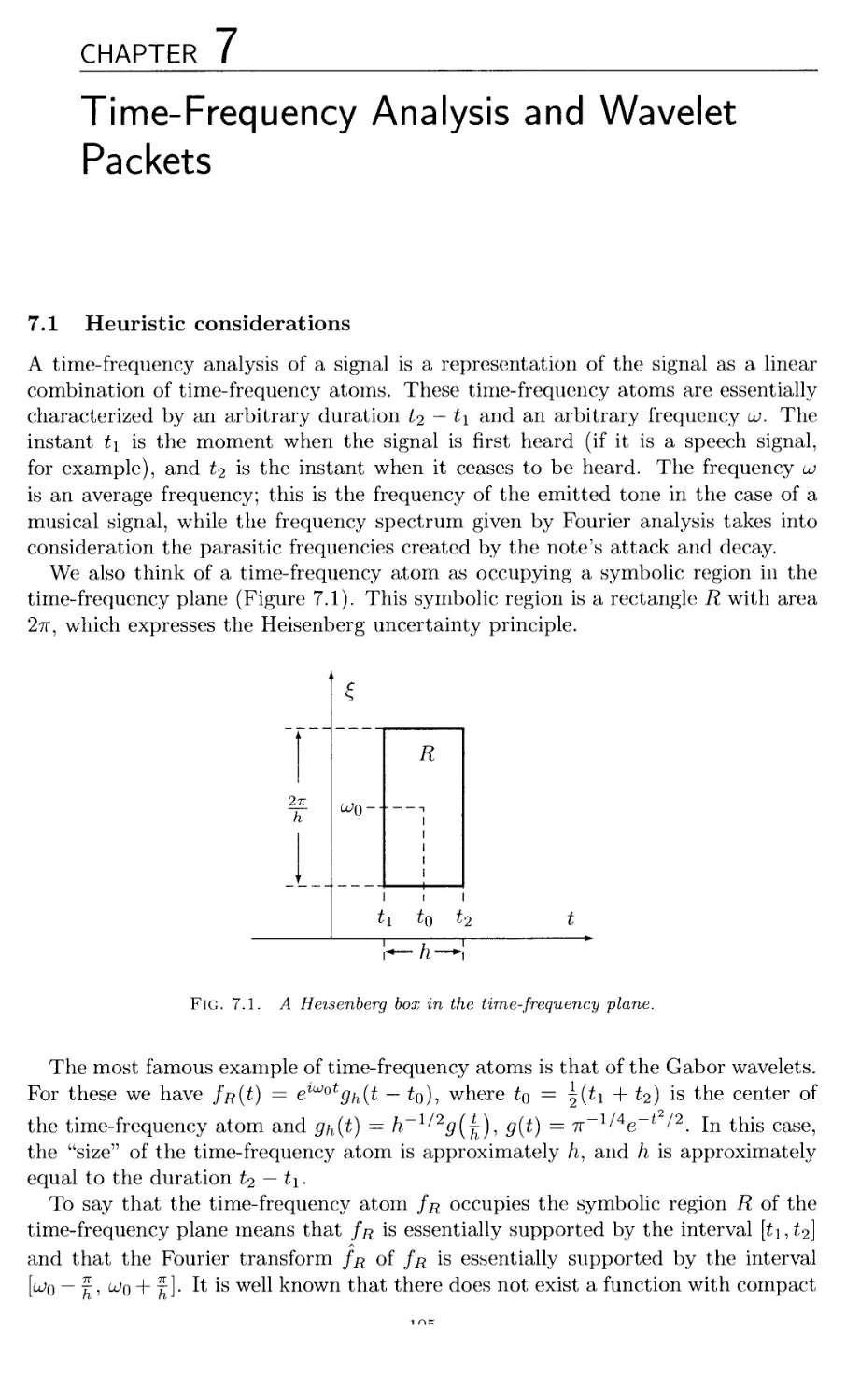
7.1	Heuristic considerations........................................105
7.2	The definition of basic wavelet packets.........................108
7.3	General wavelet packets.........................................Ill
7.4	Splitting algorithms ...........................................112
CONTENTS	vii
7.5	Conclusions......................................................114
Chapter 8.	Computer Vision and Human Vision	117
8.1	Marr’s program...................................................117
8.2	The theory of zero-crossings.....................................120
8.3	A counterexample to Marr’s conjecture............................121
8.4	Mallat’s conjecture..............................................122
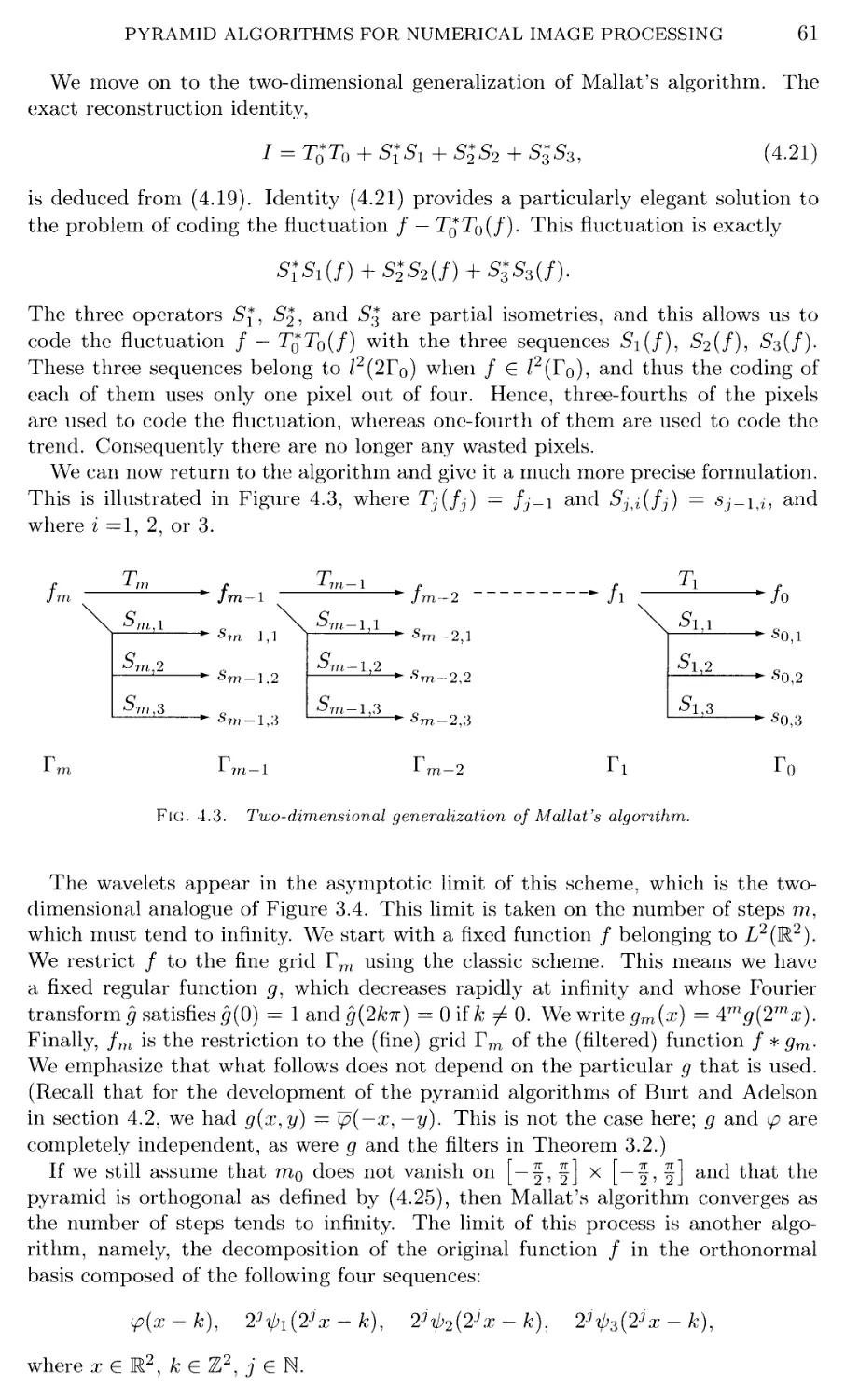
8.5	The two-dimensional version of Mallat’s algorithm................124
8.6	Conclusions......................................................125
Chapter 9.	Wavelets and Turbulence	127
9.1	Introduction.....................................................127
9.2	The statistical theory of turbulence and Fourier	analysis........128
9.3	Multifractal probability measures and turbulent	flows ...........130
9.4	Multifractal modeling of the velocity field......................131
9.5	Coherent structures .............................................137
9.6	Conder’s experiments ............................................139
9.7	Marie Farge’s numerical experiments..............................140
9.8	Modeling and detecting chirps in turbulent	flows................141
9.9	Wavelets, paraproducts, and Navier-Stokes	equations..............145
9.10	Hausdorff measure and dimension.................................147
Chapter 10.	Wavelets and Multifractal Functions	149
10.1	Introduction....................................................149
10.2	The Weierstrass function........................................150
10.3	Regular points in an irregular background.......................152
10.4	The Riemann function............................................157
10.4.1 Holder regularity at irrationals..........................158
10.4.2 Riemann’s function near xq = 1............................163
10.5	Conclusions and comments .......................................164
Chapter 11.	Data Compression and Restoration of Noisy Images 167
11.1	Introduction....................................................167
11.2	Nonlinear approximation	and	sparse	wavelet expansions...........168
11.3	Denoising.......................................................177
11.4	Modeling images.................................................181
11.5	Ridgelets ......................................................184
11.6	Conclusions.....................................................185
Chapter 12.	Wavelets and Astronomy	187
12.1	The Hubble Space	Telescope	and	deconvolving its images .........187
12.1.1 The model	............................................187
12.1.2 Discovering	and	fixing the	problem.......................188
12.1.3 IDEA......................................................189
12.2	Data compression.................................................194
12.2.1	ht.compress..............................................194
12.2.2	Smooth restoration.......................................196
12.2.3	Comments.................................................197
12.3	The hierarchical organization of the universe ..................197
12.3.1	A fractal universe .......................................200
viii
CONTENTS
12.4	Conclusions...................................................201
Appendix A.	Filter Fundamentals	203
A.l The Z2(Z) theory and definitions ..............................203
A.2 The general two-channel filter bank............................205
Appendix B.	Wavelet Transforms	209
B.l	The L2 theory ................................................209
B.2	Inversion formulas............................................210
B.2.1	L2 inversion............................................211
B.2.2	Inversion with the Lusin wavelet........................213
B.3	Generalizations...............................................215
Appendix C.	A Counterexample	219
C.l	Introduction..................................................219
C.2	The function 0................................................220
C.3	Representations of f0 * Bp and its derivatives ...............221
C.4 Hunting the zeros of (Jo * ®рУ ................................223
C.5	The functions R,	R * f)p, (Л * вРУ, and (R * 0РУ' ............225
C.6	(R * 0рУ' and (R	* 0РУ vanish at the zeros of (/0 * @рУ'......225
C.7 The behavior of (R * 6>p)'7(/o * ^)"...........................226
C.8 Remarks........................................................227
C.9 A case of perfect reconstruction...............................229
Appendix D.	Holder Spaces and Besov Spaces	233
D.l Holder spaces..................................................233
D.2 Besov spaces ..................................................234
D.3 Examples.......................................................235
Bibliography	237
Author Index	249
Subject Index	253
Preface to Revised Edition
Wavelet analysis is a branch of applied mathematics that has produced a collection
of tools designed to process certain signals and images. This new book is devoted
to describing some of these tools, their applications, and their history.
We will trace several of the technical roots of wavelet analysis, going back to
the 1930s and before. These are examples of where the mathematical techniques
that we now codify as wavelet analysis first appeared. They are for the most part
concerned with the internal structure of mathematics itself. We judge that the
applied point of view began after World War II and was embedded in a more general
philosophical context exemplified by an ambitious program called The Institute for
the Unity of Science. This “institute without walls’’ was a vision, a vision that
was shared by such prominent scientists as John von Neumann, Claude Shannon,
and Norbert Wiener. It was the time when Claude Shannon discovered the laws
that govern the coding and transmission of signals and images. It was the time
when Norbert Wiener and John von Neumann unveiled the relationships between
mathematical logic, electronics, and neurophysiology. This led to the design of the
first computers. It was the time when Dennis Gabor proposed that speech signals
should be decomposed into a series of time-frequency atoms he named "logons."
It was the time when Eugene P. Wigner and Leon Brillouin introduced the time-
frequency plane.
These pioneering scientists opened new avenues in science, and one of these av-
enues is called time-frequency analysis. Time-frequency analysis, which is based on
Gabor wavelets, will be one of the main topics of this book. Gabor wavelets were
improved by Kenneth Wilson, Henrique Malvar, and finally by Ingrid Daubechies,
Stephane Jaffard, and Jean-Lin Journe.
In contrast with this established line of research, time-scale analysis has had a
harder time. Indeed, time-frequency analysis yields the musical score, the notes
with their frequencies and durations of the music we hear. Time-scale analysis
focuses on the transients, the attack of the trumpet, which lasts a few milliseconds,
and similar nonstationary signals. While time-frequency analysis was born in the
1940s, time-scale analysis emerged in the late 1970s in completely distinct areas
such as image processing (E. H. Adelson and P. J. Burt), neurophysiology (David
Marr), quantum field theory (Roland Seneor, Jacques Magnen, Guy Battle, Paul
Federbush, James Glirnm, and Arthur Jaffe), and in geophysics (Jean Morlet). The
outstanding collaboration between Alex Grossmann and Jean Morlet gave birth to
a new vision that emerged in the 1980s, and the message was the following: While
stationary or quasi-stationary signals are adequately decomposed into a series of
time-frequency atoms or Gabor-like wavelets, signals with strong transients are
X
PREFACE TO REVISED EDITION
better analyzed with the time-scale wavelets developed by Grossmann and Morlet.
A spectacular example where time-frequency analysis and time-scale analysis
have been able to compete is the new JPEG-2000 compression standard for still
images. This new standard is based on time-scale wavelets. The old JPEG standard
was based on an algorithm called the discrete cosine transform, which is a kind of
windowed Fourier transform. This algorithm belongs to the time-frequency group.
(Here one ought to say “space-frequency,” since an image is a two-dimensional
signal.) In the case of JPEG-2000, and in similar compression problems, time-scale
wavelets have been preferred over time-frequency wavelets. This success story was
not available when the original book first appeared.
This new book began as a one-chapter revision of Wavelets: Algorithms &
Applications (SIAM, 1993), which is based on lectures Yves Meyer delivered at
the Spanish Institute in Madrid in February 1991. While Yves Meyer and Robert
Ryan were working on the translation and revision of the new chapter, which ul-
timately became Chapter 11 of the current book, it became clear, based on the
many developments in both the theory and applications since 1993, that an exten-
sive revision of the original book was needed. Since Stephane Jaffard already had
suggested a number of changes and additions, particularly in the sections involv-
ing the analysis of multifractal functions, where he is a recognized expert, he was
invited to join the project. The result of our collaboration is an almost completely
new book, and thus we have given it a new title. Although we have retained the
core of the first four chapters, many parts of these chapters have been rewritten
and expanded, particularly Chapters 1 and 2. Appendix A has been added as an
introduction to some basic filter concepts and hence as a complement to Chapter
3. Chapter 5 has been completely rewritten; it contains new material on chirps
that was not known when the first edition was published. Chapters 6 and 7 have
been slightly expanded, but they generally follow the original texts. Rather than
expanding Chapter 8, we have added Appendix C, which is devoted to a complete
discussion of a counterexample to a conjecture of Stephane Mallat on zero-crossings.
This counterexample was outlined in the first edition, but this is the first time the
details have been published.
Chapters 9 and 10, although based on the first edition, are considerably expanded
and hence essentially new. Chapter 9 (formerly Chapter 10) tells a much more
complete and up-to-date story about the use of wavelets for the study of turbulence.
Chapter 10 (based on the former Chapter 9) contains a complete analysis of the
Weierstrass and Riemann functions, plus a general discussion about the use of
wavelets to analyze multifractal functions. Appendix В complements Chapter 10
by providing key results (with proofs) about some wavelet transforms and their
inverses. The treatment here is perhaps slightly different from other developments
of this now-classical theory.
Chapter 11 is the original motivation for this new book, and we consider it
the centerpiece. Here we discuss the intriguing interaction between wavelets and
nonlinear analysis and the applications of this line of research to image compression
and denoising. Since this chapter involves the concepts that may not be familiar to
some readers, we have added Appendix D to introduce Holder and Besov spaces,
plus results on their characterizations in terms of wavelet coefficients.
The original edition contained two pages about the then-emerging use of wavelets
in astronomy. It was written at a time when the applications of wavelets to astron-
omy were received with skepticism. Wavelets are today recognized as an essential
tool in astronomy. This story has been expanded in Chapter 12, where we have
PREFACE TO REVISED EDITION
xi
written a detailed analysis of how wavelets are used in two specific algorithms. We
also discuss the use of wavelets to understand the hierarchical structure of the uni-
verse and its evolution. This is embedded in a historical context going back to the
eighteenth century.
The bibliography has been considerably expanded to include research papers from
each of the applications discussed, as well as many books and papers of general or
historical interest. We have not listed any of the many websites that exist. Instead,
we encourage the reader to visit the “official’’ wavelet site, www.wavelet.org, which
is edited by Wim Sweldens with support from Lucent Technologies. Here one will
find fists of regularly updated references, a calendar of events, finks to homepages
of researchers, and links to sites from which wavelet software can be downloaded.
Given the scope of the applications in this book, it is clear that we are not ex-
perts in each, and thus we have relied on the help of others. We wish to thank
specifically several individuals for their time, patience, and thoughtful comments:
Richard Baraniuk, Guy Battle, Albert Bijaoui, Yves Bobichon, Albert Cohen,
Joseph L. Gerver, Hamid Krim, John Rayner, Sylvie Roques, Marc Tajchman,
Bruno Torresani, and Eva Wesfreid.
Stephane Jaffard
Yves Meyer
Robert D. Ryan
Preface from the First Edition
The “theory of wavelets” stands at the intersection of the frontiers of mathematics,
scientific computing, and signal processing. Its goal is to provide a coherent set of
concepts, methods, and algorithms that are adapted to a variety of nonstationary
signals and that are also suitable for numerical signal processing.
This book results from a series of lectures that Mr. Miguel Artola Gallego, Direc-
tor of the Spanish Institute, invited me to give on wavelets and their applications.
I have tried to fulfill, in the following pages, the objective the Spanish Institute
set for me: to present to a scientific audience coming from different disciplines, the
prospects that wavelets offer for signal and image processing.
A description of the different algorithms used today under the name “wavelets”
(Chapters 2-7) will be followed by an analysis of several applications of these
methods: to numerical image processing (Chapter 8), to fractals (Chapter 9), to
turbulence (Chapter 10), and to astronomy (Chapter 11). This will take me out
of my domain; as a result, the last two chapters are merely resumes of the original
articles on which they are based.
I wish to thank the Spanish Institute for its generous hospitality as well as its
Director for his warm welcome. Additionally, I note the excellent organization by
Mr. Perdo Corpas.
My thanks go also to my Spanish friends and colleagues who took the time to
attend these lectures.
CHAPTER 1
Signals and Wavelets
The purpose of this chapter is to give the reader a fairly clear idea about the
scientific content of the book. All of the themes that will be developed in this study,
using the necessary mathematical formalism, already appear in this overture. It is
written with a concern for simplicity and clarity and avoids as much as possible the
use of formulas and symbols.
Signal and image processing ultimately involve a collection of numerical tech-
niques, or algorithms. But like all other scientific disciplines, signal and image
processing assume certain preliminary scientific conventions. We have sought in
this first chapter to describe the intellectual architecture underlying the algorith-
mic constructions that will be presented in other parts of the book.
1.1	What is a signal?
Signal processing has become an essential and ubiquitous part of contemporary
scientific and technological activity, and the signals that need to be processed appear
in most sectors of modern life. Signal processing is used in telecommunications
(telephone and television), in the transmission and analysis of satellite images, and
in medical imaging (echography, tomography, and nuclear magnetic resonance), all
of which involve the analysis, storage or transmission, and synthesis of complex
time series. Signal processing occurs in most late-model automobiles, typically for
some monitoring or control function. The record of a stock price is a signal, and so
is a record of temperature readings that permit the analysis of climatic variations
and the study of global warming.
Does there exist a definition of a signal that is appropriate for the field of sci-
entific activity called signal processing? We will not be mathematically precise on
this point; instead, we provide a working definition. A needlessly broad definition
of signal could include the sequence of letters, spaces, and punctuation marks ap-
pearing in Montaigne’s Essays, but the tools we present do not apply to such a
signal. We note, however, that the structuralist analysis done by Roland Barthes
on literary texts shares some interesting similarities with multiresolution analysis
(Chapter 4). The point of contact is the notion of scale. Barthes used the idea
of scale in his analysis of literary texts, where different scales are represented, for
example, by book, chapter, paragraph, sentence, and word. We will see that the
definition of multiresolution analysis is built on the concept of scale.
The signals we study will always be sequences of numbers and not sequences of
letters, words, or phrases. These numbers often come from measurements, which
are typically made using some recording device. We think of these signals as being
functions of time like music and speech or, in some cases, as functions of posi-
2
CHAPTER 1
tion. For example, by properly associating numbers with the four bases of a DNA
molecule, one obtains a signal that can be analyzed by the methods we describe in
Chapter 9. Here we are thinking of one-dimensional signals, functions of a single
time or space variable.
It is equally important to consider two-dimensional signals, which we call images.
Here again, image processing is done on the numerical representation of the image.
For a black and white image, the numerical representation is created by covering the
image with a sufficiently fine grid and by assigning a numerical gray scale, denoted
by f(x, y), to each grid point (x. y). The value of f(x, y) is an average of the gray
scales of the image in a neighborhood of (x,y). The image thus becomes a large
matrix, and image processing is done on this matrix.
These arrays can be enormous, and as soon as one deals with a sequence of
images, such as in television, the volume of numerical data that must be processed
becomes immense. Is it possible to reduce this volume by discovering hidden laws,
or correlations, that exist between the different pieces of numerical information
representing the image? This question leads us naturally to consider some of the
goals of the scientific discipline called signal processing.
1.2	The language and goals of signal and image processing
The subjects we are going to study appear in the scientific landscape where parts
of mathematical physics, mathematics, and signal processing intersect, and conse-
quently they share language from these disciplines. This can be confusing, so it
is useful to explain some of the terms that we will be using. In so doing, we will
introduce the signal processing tasks that appear throughout the rest of the book.
“Analysis” has the same meaning in science that it has in ordinary language.
The standard dictionary definition of “analyze” is to separate the whole (of either
a physical substance or abstract idea) into its essential parts to examine the relation-
ships between these parts as well as their relationship to the whole. The concept of
analysis provides a program of work based on this hypothesis: Behind the apparent
complexity of the world there is a hidden order that is accessible through analysis.
The complexity is due to the mixture, to the combination of simple entities. The
objective of analysis is to discover the nature of these constituents and how they
relate to one another. This program is one of the pillars of modern science.
In chemistry, this approach led to the preparation of pure substances and to the
discovery of molecules and atoms, and it continues today in particle physics. The
synthesis of urea by Friedrich Wohler in 1828 was proceeded by, and based on, its
analysis. Analysis often has the same meaning in mathematics. Take, for example,
Fourier analysis and assume that the complex object to be studied is a continuous,
27r-periodic function of a real variable. One tries to decompose the function into its
structural elements. These are the simplest of the 2?r-periodic functions, namely,
the sines and cosines. The analysis furnishes the Fourier coefficients. The analysis
is validated by a synthesis, and here the synthesis is additive. It amounts to rep-
resenting the analyzed function by its Fourier series. The synthesis is successful,
however, only after the rules for combining the components are established. In our
example, this amounts to finding a summation process that ensures the convergence
of the Fourier series furnished by the analysis.
In contrast to chemistry, where the constituent parts are well defined, Fourier
analysis is not the only way to study the properties of continuous, 2?r-periodic
functions. For example, by reinterpreting work by G. H. Hardy on a series
SIGNALS AND WAVELETS
3
attributed to Bernhard Riemann, Matthias Holschneider and Philippe Tchamitchian
have shown that wavelet analysis is more sensitive and efficient than Fourier analysis
for studying the differentiability of the Riemann function at a given point.
In Fourier analysis, the structural elements are unique; they are sines and cosines.
However, in wavelet analysis we will encounter many kinds of wavelets and other
objects, such as wavelet packets. Unlike Fourier analysis, wavelet analysis favors
no particular set of analyzing functions. There are many analyses, and we are led
to the concept of a “box of tools” containing different analytic methods. Each of
these methods provides a different way to view complexity. The choice of analytic
method is justified by the goal of the analysis.
These remarks apply particularly to signal processing. To analyze a signal means,
in this book, to look for the constituent elements. These constituent elements are
the elementary signals, the simplest signals into which the given signal can be
decomposed. But an analysis makes sense only if it enables one to understand the
properties of the object being analyzed and to understand its complexity. We will
return to this aspect of signal analysis in section 1.3, where we introduce atomic
decompositions.
The term “coding” conies from information theory and signal processing, where
it, like “analysis,” has many uses. “Transform coding” is a general term that refers
to taking a linear transform of a signal or image. Fourier analysis is a form of
transform coding, as are the algorithms discussed in Chapters 4 and 5. Note that
“coding” and “analysis” do not always refer to linear processes. The coding by zero-
crossings discussed in Chapter 8 is nonlinear. However, in each case, coding involves
methods to transform the recorded numerical signal into another representation
that is—depending on the nature of the signals studied— more convenient for some
task or further processing. Decoding is simply the inverse of coding, and it means
the same thing here as synthesis, or reconstruction.
“Transmission” and “storage” have their ordinary meanings, but in the context of
signal processing, these terms can involve layers of complexities. Every transmission
channel, whether an old telegraph line or a modern satellite link, has a definite
bandwidth and a computable cost for its use. Similarly, every storage medium
has performance limitations and a price tag. The costs of information storage and
transmission account for much of the economic motivation behind signal processing:
The goals are to provide transmission and storage at a given level of performance for
the lowest cost. Transmission and storage are often interrelated, in the sense that
what is stored must be accessed and transmitted. These ideas will be illustrated
later with examples, including the storage of fingerprints by the Federal Bureau
of Investigation (FBI) and the storage and transmission of astronomical images
(Chapter 12).
The constraints placed on transmission and storage require that information be
compressed. For example, it is too slow and too expensive to transmit raw images
over the Internet. Before being transmitted, images are compressed using one of
several schemes such as Joint Photographic Experts Group (JPEG) and Graphic
Interchange Format (GIF). Very roughly, this is how the compression we will discuss
works: A digital signal is analyzed, or coded. Either by design or luck, many of
the coefficients that come from the coding are either zero or close to zero, and
the other coefficients contain the “important information” or “significant features”
of the signal. The small coefficients are set equal to zero, and the others are
“quantized” and transmitted. These are received at the end of the channel and are
used to decode, or synthesize, the signal.
4
CHAPTER 1
It is important to note that information typically is lost when small coefficients
are set equal to zero and when the other coefficients are quantized. The trick,
however, is to do the compression is such a way that the lost information is not
noticed. If all of this is done cleverly, the reconstructed signal is, for the purposes at
hand, as good as the original. A one-dimensional example is the digital telephone:
The compression and transmission must be compatible with the 64 Kbit/second
standard, which limits without recourse the quantity of information that can be
transmitted in one second. At the same time, the quality must be such that the
person at the receiver can recognize the voice at the other end.
The compression we have just described should not be confused with another
kind of compression that is well known to Internet users, namely, the compression
of applications files. Here there must be absolutely no loss of information, and
the decompressed file must be bit-for-bit the same as the original. This kind of
compression is an example of what is called entropy coding, which is another use
of “coding.” Most, but not all, uses of “coding” refer to either transform coding or
entropy coding.
Quantization is an unavoidable (and undesirable) part of this process. Theoret-
ically, the coefficients given by a coding algorithm are arbitrary real or complex
numbers, but practically, processors have finite precision, and they produce ratio-
nal numbers whose dyadic expansions have a fixed length. The desired quality of
the restored image, the channel capacity, and the cost dictate the length of the
dyadic numbers that will be transmitted. Mapping the coefficients from the coding
algorithm into a finite number of “bins” is called quantization or, more precisely,
scalar quantization. A more sophisticated process called vector quantization maps
vectors of coefficients into “bins” in ]Rn (n-dimensional Euclidean space). We will
not be discussing quantization, but we wish to emphasize how important quantiza-
tion is to the overall efficiency of the process. Quantization is an art, and the way
it is done can “make or break” an algorithm.
In most of the cases to be discussed, the analysis and synthesis (coding and de-
coding, or reconstruction) are theoretically invertible processes: There is no loss of
information, and one obtains perfect reconstruction of the original signal. Quan-
tization, however, is not an invertible process and, unfortunately, it introduces
systematic errors known as quantization noise. It is desired that the algorithms
used for coding—taking into account the nature of the signals—reduce the effects
of quantization noise. One of the advantages of quadrature mirror filters is that
they “trap” this quantization noise inside well-defined frequency channels. These
filters will be studied in Chapter 3.
There is another aspect of the coding-transmission-decoding process that needs
to be mentioned: Having quantized the coefficients into bins, it is customary to code
the bins before transmission. This coding is entropy coding, and as indicated above,
it is completely reversible. The idea is to transmit the information as efficiently
as possible, using the statistical structure of the information to be transmitted.
Perhaps the best-known example of entropy coding is the Morse Code, which codes
the most frequently used letters with the simplest sequences of dots and dashes.
The total efficiency of a compression scheme depends on the analysis, quantization,
and entropy coding and how they work together.
In addition to transmission and storage, there is a collection of signal processing
tasks called diagnostics. Roughly speaking, this is like asking and answering a
question about a signal. For example, Does a given sample of speech belong to one
of several speakers? Or, Is an underwater acoustic signal coming from a submarine
SIGNALS AND WAVELETS
5
or a ship? For the most part, this book does not deal with diagnostics; however, a
few comments are indicated.
A diagnostic often depends on extracting a small number of significant parameters
from a signal whose complexity and size are overwhelming. Some scientists believe
that diagnostics would be easier if the signal or image has been correctly analyzed
and compressed. From this point of view, analysis and the diagnostic are naturally
related to data compression, and clearly, if this compression is done inappropriately,
it can falsify the diagnostic. In the first edition of this book, we took the position
that proper compression was relevant, or even necessary, for a given diagnostic task.
Our position has changed, based mainly on a series of lectures by David Mumford
df livered at the Institut Henri Poincare in the fall of 1998.1 We now feel that most
diagnostic tasks are related to statistical modeling of a given collection of signals
or images. Statistical modeling is an important field of research that is based on
a fascinating set of tools. However, a discussion of statistical modeling lies well
beyond the scope of this book.
Finally, we mention restoration. Signal restoration is analogous to the restoration
of old paintings. It amounts to ridding the signal of artifacts and errors, which we
call noise, and to enhancing certain aspects of the signal that have undergone at-
tenuation, deterioration, or degradation. We will discuss an application of wavelets
to signal restoration in Chapter 11.
So what are the goals of signal and image processing? Experts in signal pro-
cessing are asked to develop, for a given class of signals, algorithms that perform
certain tasks or operations. These algorithms should lead to the construction of
microprocessors, like those that exist in cell phones and automobiles, that exe-
cute these tasks automatically. Some of the important tasks have been described
above: coding, diagnostics, quantization and compression, transmission or storage,
decoding, and restoration.
We will use several examples to illustrate the nature of these operations and
the difficulties they present. It will become clear that no “universal algorithm” is
appropriate for the extreme diversity of the situations encountered. Thus, a large
part of this work is devoted to describing coding or analysis algorithms that can be
adapted to particular classes of signals that one needs to process.
Our first example illustrates restoration and diagnostic. One is interested in
splitting a signal into the sum of two terms: The first term contains the informa-
tion one wishes to recover, and the second term is the noise one wishes to erase.
The problem is the study of climatic variations and global warming. This problem
was discussed in detail by Professor Jacques-Louis Lions at the Spanish Institute
in 1990 [174]. In this example, one has fairly precise temperature measurements
from different points in the northern hemisphere that were taken over the last two
centuries, and one tries to discover if industrial activity has caused global warming.
The extreme difficulty of the problem stems from the existence of significant nat-
ural temperature fluctuations. Moreover, these fluctuations and the corresponding
climatic changes have always existed, as we have learned from paleoclimatology
[250]. Thus, to have access to the “artificial” heating of the planet resulting from
human activity and to develop a diagnostic, it is essential to analyze, and then to
“erase,” these natural fluctuations, which play the role of noise.
A more surprising example appears in neurophysiology. The optic nerve’s ca-
pacity to transmit visual information is clearly less than the volume of information
xThe ideas presented in these lectures can be found in [215] and [216].
6
CHAPTER 1
collected by all the retinal cells. Thus, there must be low-level processing of in-
formation before it transits the optic nerve. David Marr developed a theory to
understand the purpose and performance of this low-level processing, which is a
type of coding and compression [198]. We present this theory in Chapter 8.
The problems encountered in archiving data—as well as problems of transmis-
sion and reconstruction—are illustrated by the FBI’s task of storing the American
population’s fingerprints. Over 200 million fingerprint records must be stored, and
the use of inked impressions on paper cards is no longer practical. The FBI began
digitizing fingerprint records some years ago as part of a modernization program,
but due to the massive amount of data (10 megabytes per record) it was decided
that some form of compression was needed. In addition to efficient storage, it was
also important to access the fingerprint files quickly and to transmit them electron-
ically throughout the world. The goal was to be able to reconstruct the received
image on a laptop computer, and the quality of the reconstructed image had to be
such that the end user, whether a fingerprint expert or an automated fingerprint
feature extractor, would have no difficulty interpreting the image. It was decided
that coding and compression offered the only solution. Different image-compression
algorithms were tested, and a wavelet-based algorithm, a variant of one described
in Chapter 6, gave the best results, where “best” involved the speed of the algo-
rithm as well as the compression ratio and the quality of the reconstructed image.
This established the standard for fingerprint compression and reconstruction that
is used today. (For further details, see Christopher Brislawn’s paper [41].)
We have just described and illustrated some of the more important goals of signal
and image processing that focus on compression, transmission and storage, and
the attendant algorithms for coding and reconstruction. It is important to note,
however, that there are many other significant problems in signal processing that
will not be discussed. In particular, there is a vast area of signal processing based on
probability and statistics that is beyond the scope of our work. As mentioned above,
statistical modeling is crucial for high-level signal processing tasks like feature or
pattern analysis and diagnostics. This is not to say that wavelets do not or will
not play a role is this expanded arena; it is rather that here we limit ourselves, for
the most part, to a deterministic theory. The few exceptions include some notes on
Brownian motion and the appearance of noise in some of the examples.
Before leaving this section, we believe it is important to reiterate a theme hinted
at above: For the most part, we will be discussing coding algorithms and the role
wavelets play in these algorithms. These techniques are clearly important in today’s
technology, but they are only a part of the overall process. The quality of the total
process depends on blending analysis, quantization, entropy coding, transmission,
and decoding—all of which are interdependent—and ultimately, on implementing
these processes in hardware.
1.3	Stationary signals, transient signals, and adaptive coding
We have just defined a set of tasks, or operations, to be performed on signals
or images. These tasks form a coherent collection. The purpose of this book is
to describe a group of coding algorithms that have been shown, during the last
few years, to be particularly effective for compression and for analyzing certain
signals that are not stationary. We also will describe several “meta-algorithms”
that allow one to choose the coding algorithm best suited to a given signal. To
approach this problem of choosing an adaptive algorithm, we briefly classify signals
SIGNALS AND WAVELETS
7
by distinguishing stationary signals, quasi-stationary signals, and transient signals.
A signal is stationary if its properties are statistically invariant over time. A
well-known stationary signal is white noise, which in its sampled form appears as a
series of independent drawings. A stationary signal can exhibit unexpected events,
but we know in advance the probabilities of these events. These are the statistically
predictable unknowns.
The ideal tool for studying stationary signals is the Fourier transform. In
other words, stationary signals decompose canonically into linear combinations of
“waves,” that is, into sines and cosines. In the same way, some interesting classes
of signals that are not stationary decompose more naturally into linear combina-
tions of wavelets. These heuristics should not be taken too literally, since the full
class of signals that are not stationary is too large to be processed by a single
methodology. The study of nonstationary signals, where transient events appear
that cannot be predicted, even statistically with knowledge of the past, necessitates
techniques different from Fourier analysis. These techniques, which are specific to
the nonstationary character of the signal, include wavelets of the time-frequency
type and wavelets of the time-scale type. Time-frequency wavelets are suited, most
specifically, to the analysis of quasi-stationary signals, while time-scale wavelets are
adapted to signals exhibiting complicated geometrical features. Examples are edges
in images and fractal or multifractal signals.
Before defining time-frequency wavelets and time-scale wavelets, we will indicate
their common points. They belong to a more general class of algorithms that are
encountered in mathematics and in speech processing. Mathematicians speak of
atomic decompositions, while speech specialists speak of decompositions in time-
frequency atoms. The scientific reality is the same in both cases.
As we have already mentioned, an atomic decomposition consists in extracting
the simple constituents that make up a complicated mixture. Contrary to what
happens in chemistry, the “atoms” that are discovered in a signal have no physical
reality; they will depend on the point of view adopted for the analysis. These
“atoms” will be time-frequency atoms when we study quasi-stationary signals, but
they could, in other situations, be replaced by time-scale wavelets, which also are
called Grossmann Morlet wavelets.
These “atoms” or “wavelets” have no more physical existence than a specific
number system used to do some numerical computation. Each number system
has an internal coherence, but no scientific law asserts that multiplication must
necessarily be done in base 10 rather than base 2. On the other hand, we feel the
number system used by the Romans is excluded for practical reasons, since it is not
particularly suitable for multiplication.
Having different algorithms that allow us to code a signal by decomposing it
into time-frequency atoms is a somewhat similar situation. The decision to use one
or the other of these algorithms will be made by considering their “performance.”
How well they perform must be judged in terms of one of the anticipated goals of
signal processing. An algorithm that is optimal for compression can be disastrous
for analysis: A standard L2 energy criterion for the compression could cause details
that are important for the analysis to be systematically neglected.
These thoughts will be developed and clarified in sections 1.6 and 1.7. At this
point, however, we need to be more specific and define wavelets, which we do in
the next two sections.
8
CHAPTER 1
1.4	Grossmann—Morlet time-scale wavelets
Time-scale analysis—which should be called space-scale in the image case, and
which is closely related to multiresolution analysis—involves using a vast range
of scales. This notion of scale, which appropriately reminds us of cartography,
implies that the signal (or image) is replaced, at a given scale, by the best possible
approximation that can be drawn at that scale. By “traveling” from the large
scales toward the fine scales, one “zooms in” and arrives at more and more precise
representations of the given signal.
The analysis is then done by calculating the change from one scale to the next.
This produces the details that allow one, by correcting a rather crude approxima-
tion, to move toward a better quality representation. This algorithmic scheme is
called multiresolution analysis and is developed in Chapters 3 and 4. Multires-
olution analysis is equivalent to an atomic decomposition where the atoms are
wavelets.
We define these wavelets by starting with a function -0 of the real variable t.
This function is called a mother wavelet if it is well localized and oscillating. (It
resembles a wave because it oscillates, and it is a wavelet because it is localized.)
The localization condition is expressed in the usual way by saying that the function
decreases rapidly to zero as \t\ tends to infinity. The second condition suggests
that -0 vibrates like a wave. Mathematically, we require that the integral of ip be
zero and that the other first m moments of ip also vanish. This is expressed by the
relations
y* tnip(t) dt = 0 for n = 0,1,..., m — 1.	(1-1)
The mother wavelet ip generates the other wavelets of the family ip(a,b)i a > 0,
b E 1R, by change of scale and translation in time. (The scale of ip is conventionally
one, and that of ip(a,b) is a > 0; the function ip is conventionally centered around
zero, and ip(a,b) is then centered around 6.) Thus we have
^(a,b)(t) = ~y= m-—- ) , a > 0,	(1.2)
va \ a /
Alex Grossmann and Jean Morlet showed in the early 1980s that this collection
can be used as if it were an orthonormal basis when ip is real-valued [133]. This
means that any signal of finite energy can be represented as a linear combination of
wavelets ip(a,b) and that the coefficients of this combination are, up to a normalizing
factor, the scalar products f(t)ip^a b^(t)dt. These scalar products measure, in
some sense, the fluctuations of the signal f around the point b, at the scale given
by a > 0.
It required uncommon scientific intuition to assert, as Grossmann and Morlet
did, that this new method of time-scale analysis was suitable for the analysis and
synthesis of transient signals. Signal processing experts were at first annoyed by
the intrusion of these two poachers on their preserve and made fun of their claims.
This polemic had a short life, and in fact, the argument should never have arisen
because the methods of time-scale or multiresolution analysis had existed for five or
six years under various disguises: in signal analysis under the name of quadrature
mirror filters and in image analysis under the name of pyramid algorithms.
The first to report on this was Stephane Mallat. He constructed a guide that
allowed the same signal analysis method to be recognized under very different pre-
SIGNALS AND WAVELETS
9
sentations, including wavelets, pyramid algorithms, quadrature mirror filters, and
Littlewood-Paley analysis. Mallat’s brilliant observations led to the mathematical
definition of multiresolution analysis, which provides a theoretical umbrella for our
subject.
Ingrid Daubechies discovered orthonormal wavelet bases having preselected reg-
ularity and compact support [71] (see also [73]). The only previously known case
was the Haar system (1909), which is not regular. Thus almost 80 years separated
Alfred Haar’s work and its natural extension by Daubechies. On the other hand,
the wavelets invented by Daubechies—or more precisely the biorthogonal versions
developed slightly later—have taken less than 10 years to enter the mainstream of
technology. The construction of Daubechies wavelets will be discussed in Chapter 3
and biorthogonal wavelets will be discussed in Chapter 4. The relevance of having
smooth wavelets will be explained in Chapter 2.
1.5	Time-frequency wavelets from Gabor to Malvar and Wilson
Dennis Gabor, in 1946, was the first to introduce time-frequency wavelets [124],
and the functions he used are called Gabor wavelets. He had the idea to divide
a wave—whose mathematical representation is cos(cj£ + 99)—into segments and to
use one of these segments as the analyzing function. This was a piece of a wave, or
a wavelet, which had a beginning and an end.
To use a musical analogy, a wave corresponds to a note (A 440, for example)
that has been emitted since the origin of time and continues indefinitely, without
attenuation, until the end of time. A wavelet then corresponds to the same A 440
that is struck at a certain moment, say, on a piano, and is later muffled by the
pedal. In other words, a Gabor wavelet has (at least) three pieces of information:
a beginning, an end, and a specific frequency in between.
Difficulties appeared when it was necessary to decompose a signal using Gabor
wavelets. As long as one does only continuous decompositions (using all frequencies
and all time), Gabor wavelets can be used as if they formed an orthonormal basis,
in the same sense described above for the Grossmann-Morlet wavelets. There are
problems, however, with a direct discrete version of the Gabor decomposition. In
the late 1940s, a number of investigators, including Leon Brillouin, Dennis Gabor,
and John von Neumann, felt that the system e27Vlkxg(x — I), k,l E Z, where g
is the Gaussian g(x) = 7г-1/4е-а: /2, could be used as a basis to decompose any
function in L2(R) (see [40], for example). Two physicists, Roger Balian (1981 in
[17]) and Francis Low (1985 in [177]), proved independently that this is not the
case. Furthermore, the Balian-Low theorem shows that the particular choice of g
is not the problem and that the result cannot be true for any smooth, well-localized
function.
It is only recently, by abandoning Gabor’s approach, that two scientists working
in different fields and in different parts of the world—Henrique Malvar in signal
processing in Brasilia and Kenneth Wilson in physics at Cornell University—have
discovered time-frequency wavelets having good algorithmic qualities. These special
time-frequency wavelets, which we call Malvar-Wilson wavelets, are particularly
well suited for coding speech and music.
The decomposition of a signal in an orthonormal basis of Malvar-Wilson wavelets
imitates writing music using a musical score. But this comparison is misleading be-
cause a piece of music can be written in only one way, whereas there exists a non-
denumerable infinity of orthonormal bases of Malvar-Wilson wavelets. Choosing
10
CHAPTER 1
one of these is equivalent to segmenting the given signal and then doing a tradi-
tional Fourier analysis on the delimited pieces. What is the best way to choose this
segmentation? This question leads us naturally to the next section.
1.6	Optimal algorithms in signal processing
Which wavelet to choose? This question has often been posed at meetings held since
1985 on wavelets and their applications. But this question needs to be sharpened.
What freedom of choice is at our disposal? What are the objectives of the choices
we make? Can we make better use of the choices offered to us by considering the
anticipated goals? These are several of the questions we will try to answer.
The goal we have in mind is aptly illustrated by a remark Benoit Mandelbrot
made in an interview on the French radio program France Culture. He noted that
“the world around us is very complicated” and that “the tools at our disposal to
describe it are very weak.” It is notable that Mandelbrot used the word “describe”
and not “explain” or “interpret.” We are going to follow him in this, ostensibly,
very modest approach. This is our answer to the problem about the objectives of
the choices: Wavelets, whether they are of the time-scale or time-frequency type,
will be chosen to describe as well as possible the reality around us. This description
may lead to scientific understanding and the formulation of scientific laws, but once
formulated, the wavelets themselves disappear. We have no reason to believe that
there are scientific laws that are written in terms of wavelets.
Thus our task is to optimize the description. This means that we must make
the best use of the resources allocated to us -for example, the number of available
bits —to obtain the most precise possible description. To resolve this problem, we
must first indicate how the quality of the description will be judged. Most often, the
criteria used are mathematical and do not have much to do with the user’s point of
view. For example, in image processing, most calculations forjudging the quality of
the description use the quadratic mean value of gray levels. It is clear, however, that
our eye is much more sensitive and selective than this quadratic measure. Thus,
in the last analysis, we should submit the performance of an “optimal algorithm”
to the users, since the average approximation criterion that leads to this algorithm
will often be inadequate.
The case of speech (telephonic communication) or music is similar. The system-
atic research that optimizes the reception quality is based on an L2 criterion that
is mathematically convenient, but it is surely not the criterion used by the human
ear.
Ideally, we should have a two-stage program: the first based on mathematical
criteria and the second based on user satisfaction. For the most part, the only
stage we describe is the “objective search” for an optimal algorithm, even though
its optimality is defined in terms of a debatable energy criterion. The search for
mathematically tractable criteria that capture the performance of the human eye
or ear continues as an open problem at the interface between mathematics and
physiology. Progress has been made in this area, and we will discuss in Chapter
11 some new criteria that seem to be closer to the user’s point of view (at least
for image processing) than the classical energy criteria. For example, in image
synthesis, these criteria favor the reconstruction of sharp edges, which the eye is
very quick to discern.
Rather than formulate ad hoc algorithms for each signal or each class of signals,
we will construct, once and for all, a vast collection called a library of algorithms.
SIGNALS AND WAVELETS
11
We also will construct a meta-algorithm whose function will be to find the particular
algorithm in the library that best serves the given signal, given the criterion for the
quality of the description.
The number of signals recorded on 210 = 1024 points that take only the two
values zero and one is 21024. It would be absurd to store all of these possible signals
in our library. We will use a very large “library” to describe the signals, but we
exclude this “library of Babel,” which would contain all the books, or all the signals
in our case. But as everyone knows, the search for a specific book in the library of
Babel is an insurmountable task. The “ideal library” must be sufficiently rich to
suit all transient signals, but the “books” must be easily accessible.
While a single algorithm, Fourier analysis, is appropriate for all stationary signals,
the transient signals are so rich and complex that a single analysis method, whether
of time-scale or time-frequency, cannot serve them all.
If we stay in the relatively narrow environment of Grossmann-Morlet wavelets,
also called time-scale algorithms, we have only two ways to adapt the algorithm to
the signal being studied: We can choose one or another analyzing wavelet, and we
can use either the continuous or the discrete version of the wavelets. For example,
we can require the analyzing wavelet ip to be an analytic signal, which means that
its Fourier transform ippF) is zero for negative frequencies. In this case, all the
wavelets a > 0, b 6 ]R, generated by also will have this property, and their
linear combinations given by the algorithm will be the analytic signal F associated
with the real signal f. (For information about analytic signals see sections 2.6 and
2.7 or [222].)
Similarly, we can follow Daubechies and for a given r > 1, choose for ip a real-
valued function in the class Cr with compact support such that the collection
2j/2V’(2jz — A:), j,k € Z, is an orthonormal basis for L2(]R). In this discrete version
of the algorithm, a = 2-J and b = A:2~-7. j, к 6 Z.
In spite of this, the choices that can be made from the set of time-scale wavelets
remain limited. The search for optimal algorithms leads us on some remarkable
algorithmic adventures, where time-scale wavelets and time-frequency wavelets are
in competition, and where they also are compared with intermediate algorithms
that mix the two extreme forms of analysis.
These considerations are developed in Chapters 6 and 7 and the question asked
some years ago—Which wavelet to choose?—seems no longer relevant. The choices
that we can and must consider no longer involve only the analyzing instrument,
which is the wavelet. They also involve the methodology employed, which can be
a time-scale algorithm, a time-frequency algorithm, or an intermediate algorithm.
Today, the competing algorithms, time-scale and time-frequency, are included in
a whole universe of intermediate algorithms. An entropy criterion permits us to
choose the algorithm that optimizes the description of the given signal within the
given bit allocation.
Each algorithm is presented in terms of a particular orthogonal basis. We can
compare searching for the optimal algorithm to searching for the best point of view,
or best perspective, to look at a statue in a museum. Each point of view reveals
certain parts of the statue and obscures others. We change our point of view to find
the best one by going around the statue. In effect, we make a rotation; we change
the orthonormal basis of reference to find the optimal basis. These reflections lead
us quite naturally to the scientific thoughts of David Marr.
12
CHAPTER 1
1.7	Optimal representation according to Marr
David Marr was fascinated by the complex relations that exist between the choice
of a representation of a signal and the nature of the operations or transformations
that such a representation permits. He wrote [198, pp. 20-21]:
A representation is a formal system for making explicit certain en-
tities or types of information, together with a specification of how the
system does this. And I shall call the result of using a representation to
describe a given entity a description of the entity in that representation.
For example, the Arabic, Roman and binary numerical systems are
all formal systems for representing numbers. The Arabic representation
consists of a string of symbols drawn from the set (0, 1, 2, 3, 4, 5, 6,
7, 8, 9), and the rule for constructing the description of a particular
integer n is that one decomposes n into a sum of multiples of powers of
10... .
A musical score provides a way of representing a symphony; the
alphabet allows the construction of a written representation of words;
and so forth. ...
A representation, therefore, is not a foreign idea at all—we all use
representations all the time. However, the notion that one can capture
some aspect of reality by making a description of it using a symbol and
that to do so can be useful seems to me a fascinating and powerful idea.
But even the simple examples we have discussed introduce some rather
general and important issues that arise whenever one chooses to use
one particular representation. For example, if one chooses the Arabic
numerical representation, it is easy to discover whether a number is a
power of 10 but difficult to discover whether it is a power of 2. If one
chooses the binary representation, the situation is reversed. Thus, there
is a trade-off; any particular representation makes certain information
explicit at the expense of information that is pushed into the background
and may be quite hard to recover.2
This issue is important, because how information is presented can
greatly affect how easy it is to do different things with it. This is evident
even from our numbers example: It is easy to add, to subtract, and even
to multiply if the Arabic or binary representations are used, but it is not
at all easy to do these things—especially multiplication—with Roman
numerals. This is a key reason why the Roman culture failed to develop
mathematics in the way the earlier Arabic cultures had.
There is an essential difference between Marr’s considerations and the algorithms
that we develop in the first six chapters. The difference is that the choice of the
best representation, according to Marr, is tied to an objective goal. For the problem
posed by vision, one goal is to extract the contours, recognize the edges of objects,
delimit them, and understand their three-dimensional organization. In contrast,
the algorithms we present in this book are aimed only at reducing the amount
of data. They were not designed to extract patterns or solve important scientific
issues; sometimes they do. One can argue that compression is a necessary first step
toward feature extraction and, conversely, that obtaining the “important features”
2These last italics are ours.
SIGNALS AND WAVELETS
13
of an image is indeed a form of compression. We, however, strongly believe that
pattern recognition is not related to the kind of compression being discussed here.
This position is based on our understanding of work by David Mumford.
What we have said so far concerns the use of wavelets for signal and image
processing, and indeed this is the major theme of our book. There is, however, a
slightly different point of view that focuses on wavelets techniques (analysis and
synthesis) as tools within mathematics. This aspect will appear in Chapter 10
where we illustrate the power of wavelet techniques by analyzing two examples of
fractal functions: the Weierstrass function and the Riemann function.
1.8	Terminology
The elementary constituents used for signal analysis and synthesis will be called, de-
pending on the circumstances, wavelets, time-frequency atoms, or wavelet packets.
The wavelets used will be either Grossmann-Morlet wavelets of the form
= -^=	a > 0, b e K,	(1.3)
the orthonormal wavelet bases that have the form
= 2J/V(2^ - ft), J.fcgZ,	(1.4)
or the local Fourier bases of the form
= ^(^ — 0 cos + 2) (^ ~ 0],	€ N, I 6 Z. (1-5)
In the first two cases, we will speak of time-scale algorithms; in the last case,
we will speak of time-frequency algorithms. Later we will mix the two points of
view and subject the local Fourier bases to dyadic dilations. One thus encounters
generalized time-frequency atoms. We will see in Chapter 10 (and in Appendix D)
that the orthonormal wavelet bases of the form (1.4) have special properties that
are not found in other decomposition algorithms.
We will use only two very large “libraries.” The first consists of orthonormal
bases whose elements are wavelet packets. In the second, the wavelet packets are
replaced by the generalized time-frequency atoms that we have just described.
1.9	Reader’s guide
In Chapters 2 through 7, we present the time-scale algorithms (Chapters 3 and 4)
and time-frequency algorithms (Chapters 5, 6, and 7). Chapter 2 has a special
status. We have tried to retrace some of the paths that led from Fourier analysis
(Fourier, 1807) to wavelet analysis (Calderon, 1960, and Stromberg, 1981) and to
the core of contemporary mathematics.
Quadrature mirror filters are studied in Chapter 3 in the context of problems
posed by the digital telephone. For this revised edition, we have added an ap-
pendix that contains elementary information about filters, and thus complements
Chapter 3.
The pyramid algorithms described in Chapter 4 concern numerical image pro-
cessing. They use precisely the quadrature mirror filters of Chapter 3, and they
lead either to orthogonal wavelets or to biorthogonal wavelets.
In Chapters 5 through 7, we will study time-frequency algorithms. The Wigner-
Ville transform enables the signal to be “displayed in the time-frequency plane.”
14
CHAPTER 1
After indicating the main properties of the Wigner-Ville transform, we show that it
leads to an algorithm that allows us to decompose a signal into new time-frequency
atoms named “chirplets,” which are a kind of frequency-modulated Gabor wavelet.
Two other algorithms that provide access to these “atomic decompositions” are
presented in Chapter 6 (local Fourier bases) and Chapter 7 (wavelet packets).
The first seven chapters form a coherent unit. This is not the case for the last five
chapters; each of them treats a special application of wavelets and time-scale meth-
ods. Chapter 8 deals with the possibility of coding an image using the zero-crossings
of its wavelet transform. In Chapter 9 we discuss turbulence and some of the recent
contributions wavelet analysis has made to this still-unsolved problem. This chap-
ter also serves as an introduction to multifractal analysis; indeed, this subject was
initially introduced as a tool for studying turbulence. Multifractal analysis is con-
tinued in Chapter 10, where we show how wavelet analysis can be use to determine
the Holder exponents, as a function of position, of a multifractal function. Chapter
10 contains analyses of the Weierstrass and Riemann functions. In Chapter 11 we
describe the use of wavelets for denoising signals and images. This chapter also pro-
vides a quick look at the connections between wavelets, nonlinear approximation,
and Besov spaces -a mixture of seemingly unrelated techniques that is producing
surprising and promising results. Chapter 12 is devoted to describing some the
wavelet-based techniques that are being used in astronomy.
Four appendices contain complementary material. Appendix A provides a brief
introduction to the language and theory of filters. Classical results on the continu-
ous wavelet transform and its inversion are presented in Appendix B. The results in
Appendix В apply in particular to the inversion formula used in Chapter 10 for the
analysis of Riemann’s function. Appendix C contains a presentation of a counter-
example to a conjecture about zero-crossings; thus it is properly an appendix to
Chapter 8. Although this counterexample has been known, this is the first time
that a complete account has been published. Appendix D contains the definitions
and a few basic results about Holder spaces and Besov spaces. These spaces are
used elsewhere in the book, particularly in Chapters 9 and 11.
CHAPTER 2
Wavelets from a Historical Perspective
2.1	Introduction
Time-frequency wavelets, which began with work by Dennis Gabor and by John
von Neumann in the late 1940s, have a relatively long history in signal processing.
Many of the fundamental contributions were subsequently achieved by physicists,
and here we are thinking of work by Francis Low, Roger Balian, and Kenneth
Wilson. Time-frequency wavelets have been widely used in speech processing, as
will be shown in Chapter 6. Mathematicians did not pay much attention to this
field. In contrast, the use of time-scale wavelets for signal and image processing is
relatively recent, dating from the 1980s. However, in looking back over the history
of mathematics, we will uncover at least seven different origins of wavelet analysis.
Most of this work was done around the 1930s, and at that time the separate efforts
did not appear to be parts of a coherent theory. Only today do we see how this
work fits into the history of the theory of wavelets.
We feel that it is important to describe these sources in some detail. Each of
them corresponds to a specific point of view and a particular technique, which only
now are we able to view from a common scientific perspective. What’s more, these
specific techniques were rediscovered several years ago by physicists and mathe-
maticians working on wavelets. Matthias Holschneider used, without knowing it,
Lusin’s technique (1930) to analyze Riemann’s function (sections 2.6 and 10.4).
Grossmann and Morlet rediscovered Alberto Calderon’s identity (1960) 20 years
later. And to spare no one, Yves Meyer was not the first to construct a regular,
well-localized orthonormal wavelet basis having the algorithmic structure of Haar’s
system (1909): J.-O. Stromberg had done the same thing five years earlier [245].
Does this mean that everything had already been written? Not at all. More
significantly, by rediscovering a number of known results, the “modern” wavelet
investigators gave them new life and authority. Our debt to Grossmann and Morlet
is not so much for having rediscovered Calderon’s identity as it is for having used
it to analyze nonstationary signals. This early application of wavelets to signal
processing certainly encountered resistance, and Calderon himself found this use of
his work incongruous.
The recent history of wavelets has been characterized by another phenomenon
that we find scientifically important and sociologically interesting. From the be-
ginning in the early 1980s, the “wavelet group” has consisted of researchers from
several quite different disciplines, having different cultures and problems. The ex-
changes within this group created a dynamic environment that we believe accounts
for the rapid advances seen on at least two fronts: the synthesis and structuring
of previous and new knowledge to produce a coherent theory of wavelets, and the
16
CHAPTER 2
rapid adoption of wavelet techniques in diverse disciplines outside mathematics.
Not surprisingly, the most active interface has been between mathematics and sig-
nal processing, and it can be fairly said that most applications in other fields have
been through signal or image processing. But we wish to emphasize that the “flow”
has been in both directions, and that mathematics has greatly profited by input
from the other sciences. The most spectacular example (which is described in sec-
tion 2.10) is the construction by Ingrid Daubechies of her celebrated orthonormal
bases. As will be explained, this construction benefited from work in signal pro-
cessing. Another example is Stephane Jaffard’s work on the analysis of multifractal
functions, which was influenced by work on turbulence by Alain Arneodo and his
team.
The history of wavelets is reminiscent of the recent history of fractals. Fractal
objects -long before the name was coined—appeared in mathematics more than a
century ago. Georg Cantor’s triadic set is a prime example. In the mid nineteenth
century, nobody would have suspected that fractals could be used to model natural
phenomena in physics and chemistry as initiated by Mandelbrot. The success of this
modeling led some scientists to speak about “a theory of fractals.” This theory has
been questioned with skepticism by certain mathematicians. Nevertheless, one must
acknowledge that Mandelbrot’s scientific vision has been a source of inspiration in
contemporary mathematics. At a more artificial level, both fractals and wavelets
involve “scale,” and so they enjoy a natural relationship, as we hope to show in
Chapters 9 and 10.
Our immediate objective in this chapter is to describe the links between signal
processing and the different mathematical efforts that developed outside the “theory
of wavelets”; a larger objective is to show how wavelet-based techniques in signal
processing have been applied to disciplines outside mathematics.
2.2	From Fourier (1807) to Haar (1909), frequency analysis becomes
scale analysis
We first go back to the origins, that is, to Joseph Fourier. As is well known, Fourier
asserted in 1807 that any 2?r-periodic function f could be represented by the sum
o-o + cos kx + bk sin kx),
fc=i
which is called its Fourier series. The coefficients oq, a^, and bk (к > 1) are given
by
ao = X- /	dx
Jo
and by
1	/*2 77	1
ak = —	f (ж) cos kx dx,	bk = —	/(ж) sin kxdx.
Jo	Jo
When Fourier announced his surprising results, neither the notion of function
nor that of integral had yet received a precise definition. We can say conservatively
that the mathematical justification of Fourier’s statement played an essential role
in the evolution of the ideas mathematicians have had about these concepts.3
3We recommend Fourier Series and Wavelets by J.-P. Kahane and P. G. Lemarie-Rieusset
[164] for the history of Fourier series.
WAVELETS FROM A HISTORICAL PERSPECTIVE
17
Before Fourier’s work, entire series were used to represent and manipulate func-
tions, and thus the most general functions that could be constructed were endowed
with very special properties. Furthermore, these properties were unconsciously as-
sociated with the notion of function itself. By passing from a representation of the
form
2	3
ao + aix + a,2X + a^x +   •
to one of the form
«о + («1 c°s x + b\ sin x) + (a2 cos 2x + 62 sin 2z) + • • • ,
Fourier discovered, without knowing it, a new functional universe.
In 1873, Paul Du Bois-Reymond constructed a continuous, 2?r-periodic function
of the real variable x whose Fourier series diverged at a given point. If Fourier’s
assertion were true, it could not be so in the naive sense imagined by Fourier. At
that time, three new avenues were opened to mathematicians, and all three have
led to important results:
(1)	They could modify the notion of function and find one that is adapted, in a
certain sense, to Fourier series.
(2)	They could modify the definition of convergence of Fourier series.
(3)	They could find other orthogonal systems for which the divergence phe-
nomenon discovered by Du Bois-Reymond in the case of the trigonometric
system cannot happen.
The functional concept best suited to Fourier series was created by Henri
Lebesgue. It involves the space L2[0,2tt] of functions that are square integrable
on the interval [0, 2тг]. The sequence
1	1	1	.	1	«	1	•	«	/ X
____, -y=cosa?, —2=sina;, —— cos2.r. —=sm2x, ...	(2-1)
v2tt \J 7Г	V71"	v77	V77
is an orthonormal basis for this space. Furthermore, the coefficients of the decompo-
sition in this orthonormal basis form a square-summable series, and this expresses
the conservation of energy: The quadratic mean value of the developed function /
is (up to a normalization factor) the sum of the squares of the coefficients. Finally,
the Fourier series of / converges to / in the sense of the quadratic mean.
The second way that was followed to avoid the difficulty raised by Du Bois-
Reymond was to modify the notion of convergence. If the partial sums sn are
replaced by the Cesaro sums an — ($q + • • • + sn_i)/n, then everything falls into
place: The Fourier series of a continuous function f converges uniformly to f.
The third route leads to wavelets. This was followed by Haar, who asked
himself this question in his thesis: Does there exist another orthonormal system
h0, hi,... ,hn,... of functions defined on [0,1] such that for any continuous function
f defined on [0,1], the series
(f,ho)ho(x) + (/, h^h^x) 4------H (/, hn)hn(x) H---
converges to /(a:) uniformly on [0,1]? Here we have written
{u, v) = / u(x')v(x') dx,
18
CHAPTER 2
where v(x) is the complex conjugate of v(x), and we have chosen the interval [0,1]
for convenience.
As we will see, this problem has an infinite number of solutions. In 1909, Haar
discovered the simplest solution and at the same time opened one of the routes
leading to wavelets [134].
Haar begins with the function h such that h(x) = 1 for x 6 [0, |), h(x) = — 1
for x E [|,1). and h(x) = 0 for x [0,1). For n > 1, he writes n = 27 + fc,
j > 0, 0 < A; < 27, and defines h„{x) = 23^2h(23x — k). The support of hn is
exactly the dyadic interval In — [A:2~7, (k + 1)2-J), which is included in [0,1) when
0 < к < 27. To complete the set, define ho (a?) = 1 on [0,1). Then the sequence
ho, hi,... , hn,... is an orthonormal basis (also called a Hilbert basis) for A2[0,1].
The uniform approximation of f(x) by the sequence
Sn(f)(x) = (/, h0)h0(.r) H----F {fhn)hn(x)
is nothing more than the classical approximation of a continuous function by step
functions whose values are the mean values of /(a?) on the appropriate dyadic
intervals.
We can criticize the Haar construction on a couple of points. On one hand, the
atoms hn used to construct the continuous function f are not themselves contin-
uous functions, and thus there is a lack of coherence. But there is a more serious
criticism. Suppose that instead of being continuous on the interval [0,1], f is a C1
function, which means that f is continuous and has a continuous derivative. Then
the approximation of f by step functions would be completely inappropriate. In
this case, a suitable approximation would be the one created from the graph of f
by inscribing polygonal lines.
These two defects of the Haar system and the idea of approximating the graph
of f(x) with inscribed polygonal lines led Faber and Schauder to replace the func-
tions hn of the Haar system by their primitives. This research began in 1910 and
continued until 1920.
Define the “triangle function” A by A(a?) = 0 if x [0,1], A(a?) = 2x if 0 < x <
and A(a?) = 2(1 — x) if | < x < 1. Faber [100] and Schauder [234] considered the
sequence An, n > 1, defined by
An(.x) = A(27a: — к) for n = 23 + к, j' > 0, 0 < к < 23.
The support of An is the dyadic interval In = [k2~3, (k + 1)2“7], and on this
interval, An is the primitive of hn multiplied by 2 • 2J/2.
For n — 0, we set Ao(.r) = x, and we add the function A_j(a:) = 1 to complete
the set of functions. Then the sequence A_j, Aq, ... , An,... is a Schauder basis
for the Banach space E of continuous functions on [0,1]. This means that every
continuous function f on [0,1] can be written as
f(x) = a + bx + ari An(.r)	(2.2)
n= 1
and that the series has the following properties: The convergence is uniform on
[0,1] and the coefficients are unique.
We note that the Haar system is not a Schauder basis of E because a Schauder
basis of a Banach space must be made up of vectors of that space, and the functions
hn are not continuous.
WAVELETS FROM A HISTORICAL PERSPECTIVE
19
The coefficients in (2.2) can be calculated directly by induction. We have /(0) = a
and /(1) = a + b, which gives a and b. This allows us to consider a function
/(a?) — a — bx. which is zero at x = 0 and x = 1 (and which we again denote by
/). Once this reduction is made, we have /(|) = cq, which allows us to consider a
function equal to zero at x = 0, x — and x = 1. The calculation continues with
/(|) ~ a2 and /(j) = <тз, and so on. If we do not wish to “peel” f this way, the
coefficients an can be computed directly by the formula
a„ =/((fe+|)2-J) -	+ /((&+ 1)2-J)],	(2.3)
where n = 2J + k, j > 0, and 0 < к < 2J .
We can give a further interpretation to (2.2). If, instead of being continuous, f
were in C1, then we could differentiate (2.2) term by term and obtain the expansion
of f' in the Haar basis. If f is in C1, the series (2.2) converges uniformly to f and
the series differentiated term by term converges uniformly to f. Does this mean
that the functions A„, n > 0, with the added function 1, constitute a Schauder
basis for the Banach space C71[0,1]? As before, this is not the case because the
functions An do not belong to the space in question.
Following Holder, we define the space C^fO, 1], for 0 < h < 1, by the relation
\f(x) — f(y)\ < C\x — y\h for some constant C > 0 and for all x,y 6 [0,1]. Then it
is clear from (2.3) that |qti | <	if f belongs to Ch. Since 2J < n < 2j + 1,
we can also write |c>n| < Cn~h, n > 1. The converse, although much less evident,
is nevertheless true when 0 < h < 1. It is not true if h = 1.
Physicists are interested in the Holder spaces Ch because they occur naturally
in the study of fractal structures. In fact, physicists wish to know more. They
are interested in functions f whose Holder exponents h(a?o) vary from one point to
another. This pointwise definition is slightly different: We say that f satisfies a
Holder condition of exponent /г, 0 < h < 1, at a point Xq if
\f(x) - f(x0)\ <C\x-x(}\h.	(2.4)
More generally, if m < h < m, + 1, m € N, then this definition should read
\f(x)-Pni(x-x0)\<C\x-xQ\h,	(2.5)
where Pm is a polynomial of degree m. Then the Holder exponent of f at Xq is
denoted by h(a;o) and defined to be the supremum of the h that satisfy (2.5).
Contemporary science deals with numerous physical phenomena having multi-
fractal structures. By this we mean that the Holder exponents of the function
representing the structure vary from point to point in a particularly erratic way.
To be more precise, we consider the set of points Ea where the Holder exponent
/i(a?o) takes the value a. If these Ea are fractal sets, we say that f is multifractal.
In this case, scientists are interested in determining the Hausdorff dimension d(a)
of En as a function of a. (Hausdorff dimension is defined in section 9.10.)
An example from mathematics of a multifractal object is the celebrated “non-
differentiable” function attributed to Bernhard Riemann, which is defined by
12^=1. sin(7rn2a;)/7rn2. This example illustrates the point that the Fourier series
of a function provides no directly accessible information about the function’s mul-
tifractal structure. By using the wavelets of Lusin (which we present in section
2.6), Holschneider and Tchamitchian obtained a new proof of Gerver’s theorem
20
CHAPTER 2
[127, 128], which states that Riemann’s function is differentiable at certain ratio-
nal multiples of 7? [144]. More recently, Stephane Jaffard has provided a complete
analysis of the multifractal nature of Riemann’s function using wavelet techniques
[153]. We describe this work in Chapter 10.
A second example is the signal coming from fully developed turbulence. The
multifractal structure of this signal has been studied by Alain Arneodo and his
collaborators. We present this example in Chapter 9.
Conceivably, the pointwise Holder exponents could be computed by going back
to the definition. However, the example of the Riemann function shows that such
an approach is too crude to yield practical results. Furthermore, for applications
outside mathematics, this approach offers no way to take into consideration the in-
evitable noise that alters a signal. The Schauder basis presents the same difficulties
because the calculation of the coefficients an (according to (2.3)) calls directly on
explicit values of the signal.
Today, we are fortunate to have much more subtle ways to attack this problem.
Specifically, the pointwise Holder exponents are now determined using wavelet anal-
ysis. The wavelet coefficients replace those given by formula (2.3). They are less
sensitive to noise because they measure, at different scales, the average fluctuations
of the signal. These methods will be described in Chapters 9 and 10.
2.3 New directions of the 1930s: Paul Levy and Brownian motion
Brownian motion is a random process. We will limit our discussion to the one-
dimensional case. We thus write X(t,cj) for the Brownian motion: t denotes time,
ш belongs to a probability space Q, and X(t, ш) is regarded as a real-valued function
of time depending on the parameter ш.
To obtain a realization of Brownian motion, we choose a particular orthonormal
basis Zi(t), i 6 I, for the usual Hilbert space A2(1R). Then we know that the
derivative (in the sense of distributions) ^X(t,cj) is written as
i&I
where the ^j(cj), i G I, are independent, identically distributed Gaussian random
variables with zero mean.
The problem is to choose the best possible representation of Brownian motion.
As in all signal processing problems, it is certainly advisable to have in mind what
we wish to study. If we wish to examine the spectral properties of Brownian motion,
we are led to select the Fourier representation. The real line is cut into intervals
[2Ztt, 2(Z + 1)тг], I 6 Z, and the trigonometric system is used on each of the intervals.
In its real form, this is the trigonometric system (2.1).
However, if we wish to highlight the local regularity of Brownian motion, Fourier
analysis is inadequate. On the other hand, the analysis using the Schauder basis
immediately reveals the Holder regularity CQ, a < |, of the Brownian motion
trajectories.
We start with the Haar basis for T2(1R) composed of the functions hn(t — I),
n > 0, I G Z, and expand the white noise ^X(i,cu) in this orthonormal basis. By
taking primitives, we obtain the development of Brownian motion in the Schauder
basis. To simplify matters, we restrict the discussion to Brownian motion on the
WAVELETS FROM A HISTORICAL PERSPECTIVE
21
interval [0,1]. For this case, I = 0, and
X(£,w) = g0(u)t + | y^2~j/2ffn(^)An(t),
n=l
where the gn(w) are independent, identically distributed Gaussian random variables
with mean zero and variance one. This expansion often is called the “midpoint
displacement construction.” This refers to the specific geometry of the “error term”
a(j, к)A(2JT — k) in the Schauder basis expansion. Adding this term amounts to
moving the midpoint of the preceding (piecewise affine) approximation of /(x).
This midpoint displacement is precisely a(j, k). In the case of Brownian motion,
these displacements are 2-J/2gn((u).
To verify that the function X(t,(u) belongs to the Holder space Cn for almost
all ш E Q, it is sufficient to show that 2-J/2|^n((u)| < С(ш)2~^а. If, for almost all
well, one had supn>0 |gn(a;)| < oo, then the trajectories of the Brownian motion
would almost surely belong to the space . But this is not the case, and instead
we have supn>2(|gn(^)|/n) < 00 f°r almost all w E Q. Then the criterion for
Holder regularity gives
\X(t + h, a?) — X(t, cu)| < h log
where C(iv) < oo for almost all wEd.
We see from this theorem of Paul Levy how a representation in a particular basis
can provide easy access to certain aspects of a problem. In this case, the Schauder
basis provides quick access to local regularity properties of Brownian trajectories.
As we were told by Gerard Kerkyacharian, this elegant proof was not given by Levy,
although the tools we are using were available to him. Zbigniew Ciesielski [53] was
the first to relate the midpoint displacement construction of Brownian motion to
its global regularity.
Fabrice Sellan [2] has extended this analysis to the case of fractional Brownian
motion, as it was proposed by Mandelbrot and J. W. van Ness to model certain
noise (see also [111]). He has found wavelets that, when suitably normalized, do
for fractional Brownian motion what the Schauder basis did for ordinary Brownian
motion. The coefficients in Sedan’s basis are uncorrelated Gaussians. This repre-
sentation allows one to simulate precisely and efficiently the long-range correlations
found in fractional Brownian motion. (For more about this, see the note at the
end of Chapter 4.) Albert Benassi, Stephane Jaffard, and Daniel Roux have gen-
eralized these ideas to the “elliptic Gaussian fields” [31]. This work demonstrates
that multiresolution methods are well adapted to the analysis and synthesis of some
Gaussian processes.
2.4 New directions of the 1930s: Littlewood and Paley
We have shown with the example of Brownian motion how the Schauder basis
provides direct and easy access to local regularity properties. On the other hand,
the analysis of these properties using the trigonometric system is considerably more
involved.
Similar difficulties are encountered when we try to localize the energy of a func-
tion. To be more precise, we first focus on 27r-periodic functions f and their Fourier
22
CHAPTER 2
series expansions. The integral A. JQ27r |/(x)|2 dx, which is the mean value of the en-
ergy, is given directly by the sum of the squares of the Fourier coefficients. However,
it is often important to know if the energy is concentrated around a few points or if
it is distributed over the; whole interval [0,2%]. This determination can be made by
calculating A. |/(x)|4dx or, more generally, |/(x)|pdx for 2 < p < oo.
When the energy is concentrated around a few points, this integral will be much
larger than the mean value of the energy, while it will be the same order of magni-
tude when the energy is evenly distributed. We write ||/||p = (^	|/(x)\p dx)1/13
and, for obvious reasons of homogeneity, we compare the norms ||/||p to determine
if the energy is concentrated or dispersed. But if p is different from 2, we can neither
calculate nor even estimate these norms ||/||p by examining the Fourier coefficients
of f. The information needed for this calculation is hidden in the Fourier series
of /; to reveal it, it is necessary to subject the series to manipulations that were
discovered by Littlewood and Paley as long ago as 1930.
Littlewood and Paley define the dyadic blocks Ajf by
Aj/N =	(afc cos kx + bk sin kx),
2J <fc<2' + 1
where	cos kx + 6,. sin kx) denotes the Fourier series of f. Then
/(x) = a0 + £ A.J(x),
1=0
and the fundamental result of Littlewood and Paley is that there exists for each p,
1 < p < oo, two constants Cp > cp > 0 such that
If p — 2, Cp — cp — 1, and there is equality in (2.6).
Up to this point, wavelets have not yet appeared. The path that leads from
the work of Littlewood and Paley to wavelet analysis passes through the research
done by Antoni Zygmund’s group at the University of Chicago. Zygmund and the
mathematicians around him sought to extend to n-dimensional Euclidean space the
results obtained in the one-dimensional periodic case by Littlewood and Paley.
It was at this point that a ’‘mother wavelet” 0 appeared. It is an infinitely dif-
ferentiable, rapidly decreasing function, defined on the Euclidean space IRC, whose
Fourier transform ф satisfies the following four conditions, where a is chosen by
hypothesis in the interval (0, |]:
(1)	ф(£) = 1 if 1 + a < lei < 2-2q.
(2)	'0(e) = 0 if lei < 1 - a or lei > 2 + 2a.
(3)	0(e) is infinitely differentiable on IRC.
(4)	Ж2--Ч)I2 = 1 for all ? 0.
Condition (4) is not as complicated as it appears. It is sufficient to verify it for
1 — a < |el < 2 — 2a, and then only two cases arise: If 1 — a < |e| < 1 + a,
WAVELETS FROM A HISTORICAL PERSPECTIVE
23
condition (4) reduces to |'0(^)|2 + |'0(2^)|2 = 1, while if 1 + a < |£| < 2 — 2a, it is
automatically satisfied since one term is equal to one and all the others are zero.
Condition (4) implies that the analysis of Littlewood-Paley-Stein (whose defini-
tion will be given in a moment) conserves L2 energy. In the one-dimensional case,
this same condition is satisfied by every mother wavelet having the property
that 2j/2^(2jx — kf j, к E Z, is an orthonormal basis for L2(IR). It also antici-
pates similar conditions shared by the quadrature mirror filters (Chapter 3) and
the Malvar-Wilson wavelets (Chapter 6).
The theory for IRC proceeds by setting тДДх) = 2nj'0(2JT) and replacing the
dyadic blocks of Littlewood and Paley with the convolutions — f * The
Littlewood-Paley-Stein function is defined by
Zoo	\V2
If f belongs to L2(IRC), the same is true for g, and \\f ||2 = Ц^Цг (the conservation
of energy).
If 1 < p < oo, there exist two constants Cp > cp > 0 such that for all functions
f belonging to LP(R"),
ср1Ы1р < II/lip < CpH^Hp,	(2-7)
where
/ r	\ i/p
ll/llp = I / \f(x)\pdx}
uv	/
The Littlewood Paley-Stein function g provides a method for analyzing f in
which a major role is played by the; ability to vary arbitrarily the scales used in
the analysis; by the same token, the notion of frequency plays a minor role. The
dilations of size 2J are present in the definition of the operators Aj. Neverthe-
less, conditions (1) and (2) endow these operators with a frequency content. The
sequence of operators Aj, j 6 Z, constitutes a bank of band-pass filters, oriented
on frequency intervals covering approximately one octave. Littlewood-Paley tech-
niques have been extensively developed by Stein and his collaborators. We refer to
[242], [243], and [114] for detailed descriptions of their applications in analysis.
Thanks to the work of Marr and Mallat (which we describe in Chapter 8), the
Littlewood Paley analysis provides an effective algorithm for numerical image pro-
cessing.
2.5 New directions of the 1930s: The Franklin system
In 1927, Philip Franklin, who was a professor at the Massachusetts Institute of
Technology, had the idea to create an orthonormal basis from the Schauder basis
by using the Gram-Schmidt process. This produces a sequence (/n)n>-i beginning
with /-i(.r) = 1, /о(ж) = 2v/3(t— j),..., which is an orthonormal basis for L2[0,1].
This sequence (/n)n>-i is called the Franklin system and satisfies
1	r1
fn(x)dx = / xfn(x)dx = 0 for n > 1.
Jo
The Franklin system has advantages over both the Schauder basis and the Haar
basis. It can be used to decompose any function / in L2 [0,1], which the Schauder
24
CHAPTER 2
basis does not allow, and it can be used to characterize the spaces Ca, 0 < a < 1,
by the relation \ {f, fn) \ < Cn-1/2- 3", which the Haar basis does not allow. Thus the
Franklin system works as well in relatively regular situations as it does in relatively
irregular situations.
The weakness of the Franklin basis is that it no longer has a simple algorithmic
structure. The functions of the Franklin basis, unlike those of the Haar basis or
those of the Schauder basis, are not derived from a fixed function ф by integer
translations and dyadic dilations. This defect caused the Franklin system to be
unattractive for applications.
Zbigniew Ciesielski revived the forgotten Franklin system in 1963 by showing
that it is localized [54, 55]. There exists an exponent 7 > 0 and a constant C > 0
such that
|/п(т)| < C2j/2 exp(-7|2hr - k\)
if 0 < x < 1, n = 2J + /7 0 < A; < 2J , and
< C23y/2exp(-7|2<r - A:|).
Thus, on a mathematical level, everything works as if fn(x) = 2д/2ф(2Фх — кф where
is a Lipschitz function having exponential decay.
Today we are aware of a much closer relationship between the Franklin system and
wavelets (see [150]). Asymptotically the functions of the Franklin system become
arbitrarily close to the orthonormal wavelet basis discovered by Stromberg in 1980.
In fact, for n = 2J+ к, 0 < к < 2J,
/n(x) = 2j/2-0(2Lr - к) + гп(ж)
where, for a certain constant C,
||rn(x)||2 < C(2 - x/3)d(n), d(n) = inf(fc,2J - k).	(2.8)
The function which was discovered in 1980 by Stromberg, is completely explicit.
It has the following three properties:
(1)	ф is continuous on the whole real line, it is linear on the intervals
[1,2],	[2,3],... , [Z,Z + 1],... ,
and it is linear on the intervals
Z + 1 Z
2 ’ 2
(2) \ф(х)\ <67(2-^3)14
(3) 2^2ф(23х - k), j, kEZ, is an orthonormal basis for L2(R).
Note that (2 — л/3) < 1; hence condition (2) means that ф decreases rapidly at
infinity, and (2.8) means that ||т(т)||2 is small when d(n) is large.
WAVELETS FROM A HISTORICAL PERSPECTIVE
25
2.6	New directions of the 1930s: The wavelets of Lusin
This section is in the right place historically, but scientifically it should come after
the next section, since Lusin’s work is an example of continuous wavelet expansions.
The interpretation of Lusin’s work in terms of the theory of wavelets would
probably astonish its author. But it is certainly the best reading, the one that
gives the greatest beauty to Lusin’s work. We begin by introducing the object of
Lusin’s study, namely, the Hardy spaces НР(Ж), where 1 < p < oo. Let P denote
the open, upper half-plane defined by z — x + iy and у > 0. A function f(x + iy)
belongs to HP(IR) if it is holomorphic in the half-plane P and if
/ roe	\ i/p
sup I / \f(x + iy)\p dx I < oo.	(2-9)
y>0 \J — схэ	/
When this condition is satisfied, the upper bound, taken over у > 0, is also the
limit as у tends to zero. Furthermore, /(ж + iy) converges to a function denoted by
f(x) when у tends to zero, where convergence is in the sense of the Lp norm. The
space НР(*С) can thus be identified with a closed subspace of LP(IR), which explains
the notation.
Hardy spaces play a fundamental role in signal processing. One associates with
a real-valued signal /, defined for all t e R of finite energy, the analytic signal F
for which f is the real part. By hypothesis, the energy of f is | f(t)|2 dt < oo,
and we require that F have finite energy as well. This implies that F belongs to
the Hardy space №(IR). Then F(t) = /(t) + ig(t), and the function g is the Hilbert
transform of f. For further information about analytic signals, the reader may refer
to [222]. One may also consult the remarkable exposition by Jean Ville [254].
Read in the light of the theory of wavelets, Lusin’s work concerns the analysis
and synthesis of functions in HP(R) using “atoms” or “basis elements,” which are
the elementary functions of HP(W). In fact, these are the functions (z — £)“2,
where the parameter £ = и + iv belongs to P. In Lusin’s work, the Hardy space
HP(F) was used as a tool to provide a better understanding of the LP(IR) space.
More specifically, singular operators were shown to be bounded on LP(IR) by first
studying their action on HP(W). In the latter case, such an operator is understood
through its action on the building blocks (z — С)-2, C 6 F.
Thus one wishes to obtain effective and robust representations of the functions
f in Hp(jP) of the form
f(z) = Уу* (z — C)~2O!(C) dudv,	(2-10)
where £ = u + iv and where q(£) plays the role of the coefficients. These coefficients
should be simple to calculate, and their order of magnitude should provide an
estimate of the norm of f in Lfp(R). Furthermore, we are interested in relating the
decomposition of f given by (2.10) to a wavelet decomposition as defined in the
next section.
The synthesis is obtained by the following rule. We start with an arbitrary
measurable function «(£), subject only to the following condition introduced by
Lusin: The quadratic functional A defined by
/	\ 1/2
А(ж) ~ \ I \a(u + iv)\2v~2 dudv ,
J
26
CHAPTER 2
where Г(ж) = {(«, v) 6 IR2 | v > |u — ж| }, must be such that f^o(A(x))p dx is
finite. Note that this condition involves only the modulus of the coefficients a(£).
If the integral f^(A(x))p dx is finite, then necessarily
/(ж) = (ж — С)~2<т(С) dudv
belongs to 7/p(IR), and if 1 < p < oc,
/ roo	\ i/p
\\f\\P<C(p)(J JA(xWdx) .	(2.11)
The left member of (2.11) is the norm of f in 7/p(IR), as defined by (2.9). The
estimate given by the right member of (2.11) is sometimes very crude. If, for
example, /(ж) = (ж + г)-2 and if one makes the natural choice of the Dirac measure
at the point i for a//), then the second member of (2.11) is infinite. This paradox
arises because the representation (2.10) is not unique.
To obtain a unique decomposition, which we call the natural decomposition, we
restrict the choice to q(£) = ^vf'(u + w). When we do this, the two norms
||/||p and ||Л||р become equivalent if 1 < p < oc. Today this natural choice of
coefficients has an interesting explanation. This interpretation, which depends on
the contemporary formalism of wavelet theory, is given in the following section.
2.7	Atomic decompositions from 1960 to 1980
Guido Weiss, in collaboration with Ronald Coifman, was the first to interpret, as
we have just done, Lusin’s theory in terms of atoms and atomic decompositions.
The atoms are the simplest elements of a function space, and the objective of the
theory is to find, for the usual function spaces, the atoms and the “assembly rules”
that allow one to reconstruct all the elements of the function space using these
atoms.
In the case of the holomorphic Hardy spaces of the last section, the atoms were
the functions (z — С) 2- С £ P*, and the assembly rules were given by the condition
on Lusin’s function A.
For the spaces Lp[0, 2-тг], 1 < p < oc, the atoms cannot be the functions cos kx and
sin kx, к > 1, because this choice does not lead to assembly rules that are sufficiently
simple and explicit to be useful in practice. Marcinkiewicz showed in 1938 that the
simplest atomic decomposition for the spaces Lp[0,1], 1 < p < oc, is given by
the Haar system. The Franklin basis would have served as well, and from the
scientific perspective given by wavelet theory, the Franklin basis and Littlewood-
Paley analysis are naturally related.
One of the approaches to atomic decompositions is given by Calderon’s identity.
To explain Calderon’s identity, we start with a function ф belonging to L2(IRn).
(Later in this history, Grossmann and Morlet called this function an analyzing
wavelet.) Its Fourier transform //£) is subject to the condition that
[ 1Ж)|/ = 1	(2.12)
Jo	1
for almost all £ 6 IRn. If ф belongs to L1 (IRn), condition (2.12) implies that
[ //ж) dx = 0.
WAVELETS FROM A HISTORICAL PERSPECTIVE
27
We write ф(х) — ?£( —ж), ^(ж) = t~nz£(j), and ^t(x) = t-nz£(j). Let Qt denote
the operator defined as convolution with its adjoint is the operator defined
as convolution with -0f.
Calderon’s identity is a decomposition of the identity operator, written symboli-
cally as
i= [°°QtQ^-
Jo T
This means that for all f G L2(R),
fl I
f= / <?«[«(/)] T 
Jo	1
where the limit of this improper integral is to be taken in the sense of L2(R).
Grossmann and Morlet rediscovered this identity in 1980, 20 years after the work
of Calderon. However, with this rediscovery, they gave it a different interpretation
by relating it to the coherent states of quantum mechanics [133]. They defined
wavelets (generated from the analyzing wavelet ф) by
=	—j, «>0, HR”.
\ a /
In the analysis and synthesis of an arbitrary function f belonging to L2(R7')i these
wavelets </;(a,b) are going to play the role of an orthonormal basis. The wavelet
coefficients W (a, 6) are defined by
T(fl,6) = (/,^4	(2.13)
where (u,v) = f u(x)v(x) dx. The function f is analyzed by (2.13). The synthesis
of f is given by
JV) = Г [ W(a,b^,(nM(X)db-^.	(2.14)
Jo Jr71	a
This is a linear combination of the original wavelets using the coefficients given by
the analysis.
We return to the specific case of the Hardy spaces №(R) for 1 < p < oo. The
analyzing wavelet ф(х) = ^(ж + z)”2 chosen by Lusin is the restriction to the real
axis of the function + z)-2; it is holomorphic in P and belongs to all of the
Hardy spaces. The Fourier transform of ф is ?3(£) = —2£e-‘’ for £ > 0 and ф(£) = 0
if £ < 0. Condition (2.12) is not satisfied; however, we have
Г.А	f 1 if £ > 0,
/	ivvoi2- = L .Л<п	(2-15)
Jo	‘	10 if 4 < 0.
Condition (2.15) implies that the wavelets ф(а,ь) generate H2(R) instead of L2(R)
when а > 0, b G R.
The wavelet coefficients of a function f belonging to the Hardy space №(R) are
then
W(a,b) = </, V\a,b)> = “ [	- \2 dx-
7Г J_oo (ж — b — гаф
By Cauchy’s formula, this is equal to 2iay/af'(b + ia), since f is holomorphic in P.
Thus the representation (2.14) of a function in the Hardy space №(R) coincides
with the natural representation that we defined in the preceding section.
28
CHAPTER 2
2.8	Stromberg’s wavelets
The real version of the holomorphic Hardy space H1(R) is denoted by ?Z1(IR). It
is composed of the real-valued functions и(ж) for which there exists a real-valued
function v(ж) such that и(ж) + гг?(ж) belongs to 7/1(IR). In other words, и(ж) belongs
to ?Y1(IR) if and only if и and its Hilbert transform u belong to LX(IR).
Research on atomic decompositions for the functions in the Hardy space ?Y1(IR)
takes two completely different approaches: One involves the atomic decomposition
of Coifman and Weiss, and the other concerns the search for unconditional bases
for the space H1. Here is an outline of these theories.
Coifman and Weiss showed that any function f of It1 can be written as
/(ж) =	(2-16)
k=0
where the coefficients Ад, are such that lAfc| < 00 anc^ where the functions
are atoms of H1. The conditions for a function to be an atom are the following: For
each flfc, there exists an interval Ik such that ak(x) — 0 outside of Д, |flfc(x)| < l/|7fc|
(]Ik\ is the length of Д), and ak(x)dx = 0. These three conditions imply that
the norms of the ak in 7Y1 are bounded by a fixed constant. The price to pay for
this extraordinary decomposition is that it is not given by a linear algorithm, and
this naturally raises the problem of finding one.
Finding an unconditional basis means constructing, once and for all, a sequence
of functions bk of It1 that are linearly independent, in a very strong sense, and such
that any function f of 7-f1 can be decomposed in the form
OO
/И = 52
fc=0
where the scalars (3k are defined explicitly by the formulas
(Зк = У f (x)gk(x') dx.
Here the gk are specific functions in the dual of H1; that is, they are BMO functions.
The strong independence property is this: There exists a constant C such that
if two sequences of coefficients (3k and Xk satisfy \(3k\ < |Afc| for all к, then
J2 Д6д,(ж) <C ^Xkbk(x) ,
fc=0	fc=0
where || • || is the norm of the function space It1.
Wojtaszczyk proved that the Franklin system {/n}neN without the function
/(ж) = 1 is an unconditional basis for the subspace of ?Z1(IR) composed of functions
that vanish outside the interval [0,1] [262]. Stromberg showed that the orthonor-
mal wavelet basis 2-?/2?/;(2-7ж — A;), j, к E Z, defined in section 2.5 is, in fact, an
unconditional basis for the space ?Y1(IR) [245].
Does there exist a relation between these two types of atomic decompositions?
We first point out the main difference: The decomposition (2.16) of a function is
not unique, and in some sense the atoms ak must be fitted to the function f. Thus
the decomposition algorithm is not linear. On the other hand, one way to construct
WAVELETS FROM A HISTORICAL PERSPECTIVE
29
the atoms for (2.16) is to start with the expansion of f in an orthonormal basis
of compactly supported wavelets and to group the wavelets to form the atoms.
These groups of wavelets are a little like the dyadic blocks of Littlewood and Paley;
however, in this case, they are defined by considering the moduli of the coefficients
ctj^k of this series. The interested reader is referred to [203]. (The construction of
wavelets with compact support will be developed in Chapter 3.)
2.9	A first synthesis: Wavelet analysis
Thanks to the historical perspective that we enjoy today, we can relate the Haar
system, the Littlewood-Paley decomposition (1930), the version of Franklin’s basis
given by Stromberg (1981), and Calderon’s identity (1960) to one another.
This first synthesis will be followed by a more inclusive synthesis that encom-
passes the techniques of numerical signal and image processing. This second syn-
thesis will lead to Daubechies’s orthonormal bases.
This first synthesis is based on the definition of the “wavelet” and on the concept
of “wavelet analysis.” We will see that the success of this synthesis depends on a
certain lack of specificity in the original definition. When wavelets were first defined,
mathematicians had not created a general formalism covering all of the examples we
presented above. A physicist and a geophysicist, Grossmann and Morlet, provided
a definition and a way of thinking based on physical intuition that was flexible
enough to cover all these cases. Starting with the Grossmann-Morlet definition, we
will present two other definitions and indicate how they are related.
The first definition of a wavelet, which is due to Grossmann and Morlet, is quite
broad. A wavelet is a function fi in L2(R) whose Fourier transform -0(£) satisfies
the condition IV’(^)!2^ = 1 almost everywhere.
The second definition of a wavelet is adapted to the Littlewood-Paley-Stein
theory. A wavelet is a function fi in L2(IRn) whose Fourier transform -0(£) satisfies
the condition |V,(2-3|2 = 1 almost everywhere. If fi is a wavelet in this
sense, then у/ log 2 fi satisfies the Grossmann-Morlet condition.
The third definition refers to the work of Haar and Stromberg. A wavelet is a
function fi in L2(IR) such that 23/2fi(23x — kf j, к E Z, is an orthonormal basis for
L2(IR). Such a wavelet fi necessarily satisfies the second condition.
This shows that in going from the first to the third definition we are adding more
conditions and thus narrowing the choice of functions that will be wavelets. What
we gain is a more economical (less redundant) representation of the analyzed func-
tion. In the general Grossmann-Morlet theory—which is identical to Calderon’s
theory—the wavelet analysis of a function f yields a function W(a, b) of n + 1 vari-
ables a > 0 and b 6 IRn. This function is defined by (2.13): W(a,b) = (f, fi(a,bf),
where fi(a,b)(x) = a~n^2fi(^^)^ a > 0, b E R".
In the Littlewood-Paley theory, a is replaced by 2~fi while b is denoted by x.
Thus, if Г is the multiplicative group {2~3, j E Z}, then the Littlewood-Paley
analysis is obtained by restricting the Grossmann-Morlet analysis to Г x Rn.
In the Franklin-Stromberg theory, a is replaced by 2~3 and b is replaced by k2~3,
where j, к E Z. In other words, the analysis of f in the Franklin-Stromberg basis
is obtained by restricting the Littlewood-Paley analysis to the “hyperbolic lattice”
S in (0, oc) x R consisting of the points (2~J, k2~3f fi к G Z. The logical relations
between these wavelets analyses are easy to verify.
We start with the Grossmann-Morlet analysis, which is equivalent to the
Calderon identity. This is written I = Jo°° QtQt^t > where Qt(/) = f * fit- This
30
CHAPTER 2
becomes I — ^ZZZxj hi the Littlewood-Paley theory. Indeed, if t = 2 J, then
one has Qt(f') = А7(/). Replacing t by 2~3 and the integral Jo°° u(t)y by the sum
JZZZ-^ u(2_J) is completely classic.
To relate Littlewood-Paley analysis to the analysis that is obtained using the
orthogonal wavelets of Franklin and Stromberg, we write Uj(-'r) ~ 23фф23х) and
Vb^) = 23ф(23хф where ^(ж) =	ж). We let denote the convolution
product f*ipj and A J denote the adjoint of the operator Aj : L2 (R) —> L2(IR). Then
д;(/) = f * The coefficients a(j, k) of the decomposition of f in Stromberg’s
orthonormal basis are then given by
k) — 2J/2 У /(x)U(2jt — к) dx
Thus we see that the wavelet coefficients are obtained by sampling the dyadic blocks
A*(/) on the grid 2-JZ. This sampling is consistent with Shannon’s theorem.
In all three cases, wavelet analysis is followed by a synthesis that reconstructs
f from its wavelet transform. In the case of Grossmann-Morlet wavelets, this
synthesis is given by the identity (2.14), which we rewrite here:
Г[	(2.17)
Jo JRn	a
In the case of the Littlewood-Paley analysis, the integral	is replaced, as
we have already mentioned, by the sum W(2-J) and (2.17) becomes
A'-) = E/' (Д-/)(Ь)Л(х'-<>)Л.	(2.18)
_oo Jr”
Finally, in the case of Stromberg’s orthogonal wavelets in one dimension, the last
integral becomes a sum, and (2.18) becomes
=£ isk^jAxY
The preceding arguments may seem less than exciting, since the hypotheses on
ф are designed specifically for the analysis of the space L2 of square-summable
functions. This is the setting in which Grossmann and Morlet wrote their theoretical
work. But this is evidently a sort of regression, for we have just shown that across a
century of mathematical history, wavelet analysis was created specifically to analyze
function spaces other than L2. Fourier analysis serves admirably for the analysis
of L2.
If we want wavelets to be useful for the analysis of other function spaces, it is
necessary to impose conditions on the wavelets in addition to those we have already
given. Until now we have required only that the analysis preserves energy or, equiv-
alently, that the synthesis gives an exact reconstruction (although this equivalence
is not immediately obvious). These new conditions concern the regularity of the
wavelet the decay at infinity of ф, and the number of vanishing moments of ф.
For example, we can require that ф belongs to the Schwartz class and that all of its
WAVELETS FROM A HISTORICAL PERSPECTIVE
31
moments vanish. Or, in the case of Daubechies’s wavelets, we can require that ip
has m continuous derivatives, that it has compact support, and that its first r + 1
moments vanish.
The properties of the Stromberg wavelet are intermediate: It has exponential
decay, as does its first derivative, and
xip(x)dx = 0.
These new wavelets are particularly useful. For example, the Daubechies wavelets
just mentioned can be used to analyze the functions in Ls,p, the space of functions
in Lp whose derivatives of order s < inf (r,m) are also in Lp.
2.10 The advent of signal processing
If history had stopped with this first synthesis, the Daubechies orthonormal bases,
which improve the rudimentary Haar basis, would never have been discovered. A
new start was made in 1985 by Stephane Mallat when he was still a graduate
student. Mallat discovered the similarities between the following objects:
(a)	the quadrature mirror filters, which were invented by Croisier, Esteban, and
Galand for the digital telephone;
(b)	the pyramid algorithms of Burt and Adelson, which are used in the context
of numerical image processing;
(c)	the orthonormal wavelet bases discovered by Stromberg and Meyer.
The relations between these concepts will be explained in the? next two chapters.
By using the relation between wavelets and quadrature mirror filters, Daubechies
was able to complete Haar’s work. For each integer r, Daubechies constructs an
orthonormal basis for L2(IR) of the form 2J/2ipr(2d x — k). j,k G Z, having the
following properties:
(a)	The support of ipr is the interval [0, 2r + 1].
(b)	0 = xnipr(x) dx = 0 for 0 < n < r.
(c)	Vv has qr continuous derivatives, where the constant q is about 1/5.
When r — 0, this reduces to the Haar system.
Daubechies’s wavelets provide a much more effective analysis and synthesis than
that obtained with the Haar system. If the function being analyzed has m contin-
uous derivatives, where 0 < m < r + 1, then the coefficients a(J,k) from its de-
composition in the Daubechies basis will be of the order of magnitude 2“hn+1/2)j/
while it would be of the order 2-3j/2 wjth the Haar system. This means that as
soon as the analyzed function is regular, the coefficients one keeps (those exceeding
the machine precision) will be much fewer than in the case of the Haar system.
Thus one speaks of signal compression. Furthermore, this property has a purely
local aspect because Daubechies’s wavelets have compact support.
Synthesis using Daubechies’s wavelets also gives better results than the Haar
system. In the latter case, a regular function is approximated by functions that
have strong discontinuities. This produces an annoying “blocking effect” when
images are compressed using Haar wavelets, as the reader can verify by referring
to the images of Jean Baptiste Joseph Fourier in Figure 2.1. These remarkable
qualities of Daubechies’s bases explain their undisputed success.
32
CHAPTER 2
F1G. 2.1. Jean Baptiste Joseph Fourier (1768 1830): The image on the right was produced
by analyzing the original image on the left using Haar wavelets. It was reconstructed from the
600 largest wavelet coefficients and shows the characteristic blocking effect that is the signature
of Haar compression. Courtesy of Academic des Sciences -Pans and Jean-Loup Charmat.
2.11 Conclusions
The status of wavelet analysis within mathematics is unique. Indeed, mathemati-
cians have been working on various forms of wavelet decompositions for a fairly
long time. Their goal was to provide direct and easy access to various function
spaces. But during this period, which stretches from 1909 to 1980, from Haar to
Stromberg, there was very little scientific interchange between mathematicians (of
the ‘‘Chicago School”), physicists, and experts in signal processing. Not knowing
about, tin1 mathematical developments and faced with the pressure of specific needs
within their disciplines, the last two groups were led to rediscover wavelets.
For example, Marr did not know about Calderon’s work on wavelets (dating from
1960) when he announced the hypothesis that we analyze in detail in Chapter 8.
Similarly, G. Battle and P. Federbush were not aware of Stromberg’s basis when
they needed it to do renormalization computations in quantum held theory [108]
(see also [27] and [29]). As it was stressed by Battle [28, p. 87], “The physics
community was intuitively aware of wavelets years before anything better than the
Haar basis was mathematically known to exist. This cultural knowledge dates back
to a paper by Wilson [261] on the renormalization group.” In the numerous Helds
of science and technology where wavelets appeared at the end of the 1970s, they
were handcrafted by the scientists and engineers themselves. Their use has never
resulted from proselytism by mathematicians.
Battle’s comment raises another point: We have given a brief historical review of
some of the mathematical origins of what is now known as the theory of time-scale
wavelets. This historical perspective is, however, incomplete for two reasons. First,
we focused the discussion on mathematics. We are sure that diligent detectives
could write a similar story about the appearance of wavelet techniques in physics—
WAVELETS FROM A HISTORICAL PERSPECTIVE
33
and perhaps in other fields of science. Indeed, as we have mentioned, David Marr
built his own wavelets in an image processing context, while several groups of
physicists working in quantum field theory designed ad hoc orthonormal wavelet
bases (see, for example, [108], [130], and [261]).
Second, we focused on time-scale wavelets. Furthermore, we note that time-
frequency wavelets were, for a rather long time, neglected by mathematicians.
They were, however, popular in signal processing. Indeed, computing the scalar
product between a given signal f and a Gabor wavelet g(t — т}егш1 amounts to per-
forming a windowed Fourier analysis. Moreover, Gabor wavelets were immediately
welcomed in physics and signal processing, while time-scale wavelets had a harder
time. Finally, Gabor wavelets can be described as an orbit under the action of the
Weyl-Heisenberg group, which is playing a key role in quantum mechanics. This
discussion will be postponed until Chapters 5 and 6, where the interaction between
quantum mechanics and time-frequency analysis will be studied in more detail.
Today the boundaries between mathematics and signal and image processing
have faded, and mathematics has benefited from the rediscovery of wavelets by
experts from other disciplines. The detour through signal and image processing
was the most direct path leading from the Haar basis to Daubechies’s wavelets.
CHAPTER 3
Quadrature Mirror Filters
3.1	Introduction
In his thesis, “Codage en sous-bandes: theorie et applications a la compression
numerique du signal de parole,” Claude Galand carefully described the quadra-
ture mirror filters (which he invented in collaboration with Esteban and Croisier
[68]) and their anticipated applications [125]. He also posed some very impor-
tant problems that would lead to the discovery of wavelet packets (Chapter 7) and
Malvar-Wilson wavelets (Chapter 6).
Galand’s work was motivated by the possibility of improving the digital tele-
phone, a technology that involves transmitting speech signals as sequences of 0’s
and l’s. However, as Galand remarked, these techniques extend far beyond digi-
tal speech, since facsimile, video, databases, and many other forms of information
travel over telephone lines. At present, the bit allocation used for telephone trans-
mission is the well-known 64 kilobits per second. Galand sought, by using coding
methods tailored to speech signals, to transmit speech well below this standard. To
validate the method he proposed, Galand compared it with two other techniques
for coding sampled speech: predictive coding and transform coding.
Linear prediction coding amounts to looking for the correlations between succes-
sive values of the sampled signal. These correlations are likely to occur on intervals
of the order of 20 to 30 milliseconds. This leads one to cut the sampled signal x(n)
into blocks defined by 1 < n < TV, N +1 < n < 2N, etc., and then to seek, for each
block, coefficients	1 < к < p, that minimize the quadratic mean ^2^ |e(n)|2
of the prediction errors defined by
p
e(n) = x(n) — akx(n — k).
k=i
In general, p is much smaller than N. To transmit a block x(n), it suffices to
transmit the first p values x(l),... , x(p), the p coefficients ai,... ,ap, and the
prediction errors e(n). The method is efficient if most of the prediction errors are
near zero. When they fall below a certain threshold, they are not transmitted, and
significant compression can result.
A form of transform coding consists of cutting the sampled signal into successive
blocks of length TV, as we have just done, and then using a unitary transformation
A to transform each block (denoted by X) into another block (denoted by Y). The
block Y is then quantized, with the hope that, for a suitable linear transformation,
the Y blocks will have a simpler structure than the X blocks. Subband coding will
be presented in the next section.
36
CHAPTER 3
For a stationary Gaussian signal, the theoretical limits of the minimal distortion
that can be obtained by the three methods are the same. However, as Galand
showed, this assumes, in the case of subband coding, that the width of the frequency
channels tends to zero and that their number tends to infinity. In Galand’s work,
these frequency channels are obtained through a treelike arrangement of quadrature
mirror filters. This construction leads precisely to wavelet packets, which we discuss
in detail in Chapter 7. Today we know that wavelet packets based on filters with
finite length do not enjoy the frequency localization that Galand had hoped for.
In the cases of linear prediction coding and transform coding, the theoretical
limits of the minimal distortion are calculated as the lengths of the blocks tend to
infinity, while conserving the stationarity hypothesis.
If the three types of coding yield asymptotically the same quality of compression,
why introduce subband coding? Galand saw two advantages: the simplicity of the
algorithm and the possibility that subband coding would reduce the unpleasant
effects of quantization noise as perceived at the receiver. By quantizing inside each
subband, the signal would tend to mask the quantization noise, and it would be
less apparent.
The same argument has been repeated by Adelson, Hingorani, and Simoncelli for
numerical image processing [3]. The use of pyramid algorithms and wavelets allows
aspects of the human visual system to be taken into account so that the signal
masks the noise. The perceptual quality of the reconstructed image is improved
even though the theoretical compression calculations do not distinguish this method
from the others. It should be observed, however, that these theoretical compression
calculations are based on a very specific hypothesis that is clearly not fulfilled in
the case of images, which are not well modeled by a Gaussian stationary processes
(see, for example, [95]).
Readers not familiar with the theory of filters may wish to look at Appendix A;
it provides an elementary introduction to the language and notation that is used
in this chapter.
3.2	Subband coding: The case of ideal filters
To illustrate the ideas, we follow Galand and begin with a simplistic example. For
a fixed m > 2, let I denote an interval of length within [0,2тг], and let ij denote
the Hilbert space of sequence (с^)^е^ satisfying lcfc|2 < oo and such that
/(0) =	is zero outside the interval I. This subspace Z2 will be called a
frequency channel.
If	is a sequence belonging to Z2, the subsequence (ckm)kez provides an
optimal, compact representation of the original. In fact, for 6 E I,
= -
m m
\ m /	\	m /

since f(0) = 0 for 0^1. Thus we have ^[ZZZx.. |cfcm|2 = A |cfc|2, and this
relation expresses the redundancy contained in the original sequence (c^), which is
strongly correlated. This means that the original sequence contains m times the
numerical data needed to reconstruct f on I, knowing that f vanishes outside of I.
This observation is a form of Shannon’s theorem, and the critical sampling Cfcm is
done at the Shannon-Nyquist rate.
The ideal subband coding scheme consists of first filtering the incoming signal
into m frequency channels associated with the intervals [— 27rd+i) i Q < Z < m -1,
QUADRATURE MIRROR FILTERS
37
and then subsampling the corresponding outputs, retaining only one point in m.
This operation, which consists of restricting a sequence defined on Z to mZ, is
called decim,ation and is denoted by m | 1. This ideal subband coding scheme is
illustrated in Figure 3.1.
У1(птп)--►
У2(пт)---►
ym(nm)—-
Fig. 3.1. Subband coding scheme.
The scheme for reconstructing the original signal is the dual of the analysis
scheme. We began by extending the sequences y±(nm), ... ,ym(nm) by inserting 0’s
at all integers that are not multiples of m. Next we filter this “absurd decision” by
using the adjoint filters F^.... , F^. The output returns the original signal (x(n)).
The reconstruction is illustrated in Figure 3.2.
Fig. 3.2. Reconstruction.
One can, as Galand did, hope for the best and try to replace the index functions
of the intervals [^, 27r^jl~1^] with more regular functions of the form w(mx — 2лГ),
0 < I < m — 1. If the w(x) = wm(a?) were a finite trigonometric sum, then the
filters Fi,... , Fm would have finite length, which is essential for applications. But
the Balian-Low theorem (Chapter 6) tells us that such a function w cannot be
constructed if we demand that it be regular and well localized (uniformly in m).
Consequently, it is not possible to realize the ideal subband coding scheme just
described if we require that the filters Fi,... , Fm have finite length and, at the
same time, provide good frequency definition.
3.3	Quadrature mirror filters
Faced with the impossibility of realizing subband coding using m bands covering
the frequency space regularly and having finite-length filters—whose length must be
Cm, for some C > 0, as required by the Heisenberg uncertainty principle—Galand
limited himself to the case m = 2. He then had the idea to effect a finer frequency
38
CHAPTER 3
tiling by suitably iterating the two-band process. We will see in Chapter 7 that
this arborescent scheme leads directly to wavelet packets, but we will also see that
these wavelet packets do not have the desired spectral properties. Subband coding
using two frequency channels works perfectly. We are going to describe it in detail.
The input signals are arbitrary sequences (x(n))nez with finite energy:
52 Ип)|2 <
which means that x G Z2(Z). In the context of the digital telephone, we assume
that the original speech signals have been sampled to give the signals (x(n))nez-
Let D denote the decimation operator D : Z2(Z) —> Z2(2Z) that consists of retain-
ing only the terms with even index in a sequence (x(n))nez- (D is also denoted by
2 | 1.) The adjoint operator
£ = £>*: Z2(2Z)	Z2(Z)
is the crudest possible extension operator. It consists, starting with a sequence
(x(2n))nez, hi constructing the sequence defined on Z obtained by inserting 0’s at
the odd indices. Thus we get the sequence
(... , 0, ж(-4), 0, a?(—2), 0, x(0), 0, x(2), 0, x(4), 0,...).
To simplify the notation we write X in place of (x(n))nez- These input signals X
are first filtered using two filters Fq and Fl. Later, we will require that Fq be a
low-pass filter (in a sense that will be made precise), and, consequently, Fl will be
a high-pass filter. However, there is no distinction between the two filters at this
point.
The outputs Xq = Fq(X) and Xl = Fl(X) are two signals (.r0(n))„ez and
(^i(n))nez with finite energy.
Xq and Xi are subsampled with the decimation operator D = 2 | 1. Then we
have To = £>(X0) = (x0(2n))nez and Tx = £>(Xx) = (.-r1(2n))neZ-
We write
(oo	X1/2	/ oo	X1/2
£|x-o(2n)|4 and ||П||=	.
The two filters Fq and Fl are called quadrature mirror filters if, for all signals X
of finite energy, one has
iiM2 + riii2 = imi2-	(3.i)
Denote the operator DFq : Z2(Z) I2 (XL) by Tq, and similarly let Tx denote the
operator DFl : Z2(Z)	Z2(2Z). It can be shown that (3.1) is equivalent to
I = TO*TO + TX*TX.	(3.2)
In (3.2), I : Z2 (Z)	Z2(Z) is the identity operator. What is much less evident is that
the vectors To*7o(X) and T*Tx(X) are always orthogonal, which is a consequence
of the following theorem.
Theorem 3.1. Let Fq(0) and Fx(0) denote the transfer functions of the filters
Fq and Fl . Then the following two properties are equivalent to each other and to
the property expressed by (3.1):
QUADRATURE MIRROR FILTERS
39
Fo(0) F^e)
Fo(0+7r)	Fi(6»+tt)
(i) The matrix
is unitary for almost all 6 E [0, 2тг].
(ii) The operator (7b, Ti) : Z* 2(Z)	Z2(2Z) x Z2(2Z) is an isometric isomorphism.
Recall that the sequence of Fourier coefficients of the 27r-periodic function Fq(0)
is the impulse response of the filter Fq, and similarly for Fi(fT) and Fi.
Condition (3.2) is called the perfect reconstruction property. The input signal X
is the sum of two orthogonal signals TqTq(X) and TfTi (X), where the signals 7b(X)
and 7i(X) were given by the analysis. The operators Tq — FqE and Tf = F{E
arc applied to two sequences sampled on the even integers. These are first extended
in the crudest way, which is by replacing the missing values with 0’s. Next, this
seemingly nonsensical step is corrected by passing the sequences through the filters
Fq and F£, which are the adjoints of Fq and F\. The correct result is read at the
output (Figure 3.3).
analysis	synthesis
Fig. 3.3. The complete scheme, analysis and synthesis.
Condition (ii) means that quadrature mirror filters constitute orthogonal trans-
formations of a particular type, while (i) allows us to construct quadrature mirror
filters that have finite impulse response. To see this, we start with a trigonometric
polynomial
то(в') = Q() + aie10 + • • • + амем
such that |mo(#)|2 + |mo(0 + 7r)|2 = 1 for all 0. Next, we write
Fq(0) =	= v'S?%.0(7 + 4
Then it follows directly that (i) is satisfied. The following five examples illustrate
the definition of quadrature mirror filters.
The first example is essentially a counterexample because it is never used, for
a reason that will become clear later. It consists of bypassing the operators Fq
and Fi and defining Tq and Ti directly. Define Tq (X) to be the restriction of the
sequence X = (x(n))nez to the even integers, and define 7i(X) to be the restriction
of this sequence to the odd integers. This is equivalent, in our notation, to taking
Fq equal to the identity I, and to taking Fi to be the shift operator defined by
(FiX)(n) = x(n — 1). Condition (3.1) is trivially satisfied, and the unitary matrix
in (i) is
1
’1 eie '
1 -eie
2
40
CHAPTER 3
/2
1
2
e
1 — e
e
associated with this choice will be the Haar
The second example is more interesting. The filter operators are defined by
(FoX^n) =
(FiX)(n) =
The unitary matrix in (i) is
1 [1 +
2 [1 -
and the orthonormal wavelet basis
system.
The third example recaptures the ideal filters presented at the beginning of the
chapter. The 27r-periodic function mo(0) is one on [0,7г) and zero on [тг, 2тг), and
mi(0) = 1 — mo(0). As above, define Fq(F) — \/2mo(0) and Fi(F) = \/2mi(0).
In the fourth example, mo(0) becomes the characteristic function of the interval
[—when it is restricted to [—7г,7г), and mi(0) = 1 — mo(0).
The last example is a smooth modification of the preceding one. With 0 < a < ,
we ask that mo(0) be 27r-periodic, equal to one on the interval [—^ + o, — o],
equal to zero on [|+a,y - a], even, and infinitely differentiable. In addition, we
impose the condition
K(»)l2 + l"‘o(0 + A2 = i-	(3-3)
Then write mi (0) = e~ie Fiq{9 + 7r), Fo(0) = \/2 mb($), Fi(ff) = \/2 mT(0), and we
obtain two quadrature mirror filters.
3.4	Trend and fluctuation
Let H denote the Hilbert space Z2(Z) of all sequences (x(n))nez such that
^2^°^ |x(n)|2 <oo. Write Hq and Hi for the two subspaces TqTq(H) and
If Fq and Fi are quadrature mirror filters, then by Theorem 3.1, H will be the
direct orthogonal sum of Hq and Hi.
Write mo(0) =	Fq(0) and assume that то(тг) = 0 and that this zero has order
q > 1. Then |mo(#)|2 = 1 + O(|<9|2r?) and mi(0) = O(\в\д) as в tends to zero. Under
these conditions, we say that Fq is a low-pass filter and that Fi is a high-pass filter,
even though this terminology may not always be strictly justified.
When these conditions are satisfied, the trend and the fluctuation around this
trend of a signal X are defined by Xq — TqTq(X) and Xi = T^Ti^X), respectively.
Note that the trend and fluctuation are defined in terms of a given pair of filters.
They are not intrinsic properties of the function X, but they are handy heuristics.
The trend Xq = Fo*Fo(X) is generally “smoother” than X, in the sense that the
low-pass filter Fq removes high frequencies from X. In fact, one often says that Xq
is “twice as smooth as X,” which is another useful heuristic. These heuristics are
consistent with a theorem by S. Bernstein that relates the smoothness of a function
with the size of the support of its Fourier transform.
3.5	The time-scale algorithm of Mallat and the time-frequency
algorithm of Galand
It is amazing to reread Galand’s thesis in the light of present understanding. Indeed,
Galand’s goal was to obtain finer and finer frequency resolutions by appropriately
QUADRATURE MIRROR FILTERS	41
iterating the quadrature mirror filters. This is possible, however, only in the case of
the ideal filters in our third example, but we cannot use these ideal filters because
they have an infinite impulse response. In spite of this criticism, we will return to
Galand’s point of view in Chapter 7, and it will lead us to wavelet packets.
Thus we see that Galand was looking for time-frequency algorithms. But his
fundamental discovery, quadrature mirror filters, was diverted from that end by
Mallat, who used quadrature mirror filters to construct time-scale algorithms using
a hierarchical scheme.
Mallat considers an increasing sequence Tj = 2“JZ of nested grids that go from
the “fine grid” Tyv, N > 1, to the “coarse grid” Tq. The signal to be analyzed
has been sampled on the fine grid (we will come back to the sampling technique
when studying the convergence problem), and our starting point is thus a sequence
f = fo belonging to Z2(Tyv).
In addition, two quadrature mirror filters Fq and are given. (We will see later
what conditions they must satisfy.) These same filters will be used throughout the
discussion.
We process the signal f by decomposing it into Tof and T\f, which we also call
the trend and fluctuation. The trend Tof = DFof has been downsampled and
“lives” the coarser grid Tyv-i; it represents a new signal that is decomposed again
into a trend and fluctuation. The fluctuations are never analyzed in this scheme,
and the algorithm follows a “herringbone” pattern illustrated in Figure 3.4. (To
be precise, the operators Tq = DFq and Ti = DF± should have another index к to
indicate that they “live” on the grid Tyv-fc. We have used a simplified notation to
emphasize that the filters are always the same; they are just expanded at each step
to fit the coarser grid.)
Гх
Гуу-i rN_2 F/v-3	F/v-4	To
Fig. 3.4. Mallat’s algorithm.
The input signal f G Z2(Tyv) is finally represented by the sequence тт,... , ryv of
fluctuations and by the last trend fx G Z2(Fq). The transformation that maps f
onto (ri,... , ryv, /yv) is composed of a sequence of transformations, each of which is
invertible because of the perfect reconstruction property of the quadrature mirror
filters. Thus f can be computed directly from (iq,... , ryv, /yv)-
The significance of Mallat’s algorithm stems from the following observation: For
appropriate choice of the filters Fq and Fi, there are numerous cases where the
fluctuations ri,... , ryv are, at different steps, extremely small. Coding the signal
thus comes down to coding the last trend /yv as well as those coefficients of the
fluctuations that are above the threshold fixed by the quantization. Notice that the
last trend contains 2~N times less data than the input signal. If, in addition, many
of the terms in the fluctuations are essentially zero, then the amount of data that
must be stored or transmitted can be appreciably less than the data representing
42
CHAPTER 3
the original signal. In other words, there can be good compression. This remark is
the starting point of Donoho’s denoising algorithms described in Chapter 11.
3.6 Trends and fluctuations with orthonormal wavelet bases
We propose to describe the asymptotic behavior of Mallat’s algorithm as the num-
ber of stages N tends to infinity. To do this, it is first necessary to present the
continuous version of this algorithm. This involves orthonormal wavelet bases in
the following “complete form,” which means that we have a wavelet plus a mul-
tiresolution analysis. This will be explained here for L2(IR), and it will be discussed
again in the next chapter for L2(IRn), where we formally define a multiresolution
analysis.
We begin with a function tp belonging to L2(IR) that has the following property:
<p(x — A:), A: G Z, is an orthonormal sequence in L2(IR).	(3-4)
Let Vo denote the closed linear subspace of L2(IR) generated by this sequence. For
the other j G Z, define the spaces Vj in terms of Vo by simply changing scale. This
means that
/(x)GVo^/(^)GV,-.	(3.5)
The other hypotheses are these: The Vj, j G Z, form a nested sequence: their
intersection	reduces to {0}; and their union UT^Vj is dense in L2(IR). We
then write p>j.k(x) = 2J/2tp(2:>x — k), j, к G Z, and define the trend fj, at scale 2~J,
of a function f G L2(IR) by
kez
The fluctuations- or details in the case of an image—are denoted by d) and
defined by dj(x) = fj+i(x) — fj(x). To analyze these details further, we let Wt
denote the orthogonal complement of Vj in V}+i, so that = Vj ф Wr Then
there exists at least one function ф belonging to Wq such that ф(х — A:), к G Z, is
an orthonormal basis of IVq. Such a function ф>, called the mother wavelet, has the
following properties:
V3,k(x) = 2j^V(2Jx - V), j, к G Z,	(3.6)
is an orthonormal basis for L2(IR), and, more precisely, for all j G Z, we have
dAx) =	(3-7)
fcGZ
The details at a given scale are thus linear combinations of the “elementary fluctu-
ations,” which are the wavelets related to that scale.
Given two functions 99 and ф that satisfy the conditions just described (which
are called the father wavelet and mother wavelet, respectively), it is possible to
define two quadrature mirror filters Fo and by using the operators To = DFt}
and T\ = DFi. This is done by relating the approximation of the function space
L2(IR) that is given by the nested sequence of subspaces Vj to the approximation
of the real line IR that is given by the nested sequence of grids Tj = 2_JZ.
QUADRATURE MIRROR FILTERS
43
To do this, we consider that the function QJ?fc(x) = 2?/2^(2-7x — k) is centered
around the point k2~i, which would be the case if q were an even function. We
associate the point k2~i with the function ipj,k- This gives a correspondence be-
tween Tj and the orthonormal basis {Qj.fc, к E Z} of Vj. At the same time, /2(Г^)
is identified isometrically with Vj.
To define the operator Tq : I2 (Tj+i) —> Z2 (Г7), it is sufficient to define its adjoint
T* :/2(Г7) —Z2(Tj+1). It is constructed by starting with the isometric embedding
Vj C Vj+i and by identifying Vj with Z2(F7) and Vj+i with /2(Tj+i), as explained
above. This adjoint T(* is a partial isometry.
The orthonormal basis ikj,k of ITj allows us to identify W, with /2(Г7) in the same
way. The isometric embedding of ITj C V}+i, interpreted with this identification,
becomes the partial isometry
Tf:/2^)-/2^).
(A mapping T : H\ —> H? from one Hilbert space to another is called a partial
isometry if ||Tx||h2 = ||т-Цн1 for all x E Hi, which is equivalent to saying T
preserves inner products; that is, (Tx, Ty)H2 = (x, у)нг for all x,y E Hi. “Partial”
means there is no assumption that the mapping is onto.)
Finally, the couple (q, -0) is represented by the couple (Tq,Ti) or, which amounts
to the same thing, by the pair (Fq, Fi) of the two quadrature mirror filters. This
crucial observation is due to Mallat.
Mallat also posed the converse problem: Given two quadrature mirror filters Fo
and Fi, is it possible to associate with them two functions q and ф having properties
(3.4), (3.5), and (3.6)? Although the converse is incorrect in general, it is correct
in numerous cases, and this led to the construction of Daubechies’s wavelets.
Our first and third examples of quadrature mirror filters show that the converse is
generally false. There are no functions q and ф behind these numerical algorithms.
The second example is related to the Haar system. The function q is the char-
acteristic function of [0,1), and Vj is composed of step functions that are constant
on each interval [&2--7, (к + 1)2“j), к E Z.
The fourth example leads to Shannon’s wavelets. The function p is the cardinal
sine defined by sin .
Finally, the last example is more interesting because both of the functions q and
ф belong to the Schwartz class <S(1R), which consists of the infinitely differentiable
functions that decrease rapidly at infinity.
In the next section, we are going to pass from the analysis of sampled functions
to the analysis of functions defined on Ж by passing to the limit in the discrete
algorithms. To do this, we will give sufficient conditions on the transfer function
Fo(0) = y/2mo(0) to construct a multiresolution analysis starting with two quadra-
ture mirror filters Fo and Fi.
3.7 Convergence to wavelets
Before one can restrict a very irregular function f belonging to L2(R) to a grid
Г = hZ, h > 0, it is often necessary to smooth the function by filtering. This
filtering ought to be done according to specific rules. These rules are designed so
that in the event f is very regular, f can be reconstructed from the sampled version
with good accuracy using interpolation. The proper sampling technique is a direct
consequence of Shannon’s work.
44
CHAPTER 3
We filter f by forming the convolution f * gh, where gtfix) = hr1 gfii-1 x) and
where g is chosen so that it and its Fourier transform g satisfy the following three
conditions:
(1)	g E Cr and g,g',... , all decrease rapidly at infinity.
(2)	g(x) dx — 1.
(3)	д(2ктг) = 0 for к E Z, к 0.
One can then restrict the filtered signal f * gh to the grid hZ.
We assume that these conditions are satisfied throughout the discussion, and
we begin by reconsidering Mallat’s “herringbone” algorithm. Start by fixing f in
L2(R) and sample f on the grid Гдг using the preconditioning filter f * gN, where
gN(x) = 2Ng(2Nx).
We wish to study the asymptotic behavior of Mallat’s algorithm as N tends to
infinity. The limit we are looking for is defined as follows: Fix the index j of the grid
Tj. (Starting with Го, we will look at Г1,Г2,Гз,... .) Then we seek the (simple)
limits of the sequences
/а(А:),глг(А:),глг_1(2_1Л;), ... , rN-j (2“7/c),. . .
as N tends to infinity, j and к being fixed. Refer to the “herringbone” scheme
(section 3.5 and Figure 3.4) for the definitions of fN,r^,r^-i,.... Here are the
results [210], which do not depend on the choice of g as long as it satisfies the
conditions stated above. (We note that this last point will come up again in Chapter
4 when presenting the two-dimensional version of this theorem.)
Theorem 3.2. Assume that the impulse responses of the quadrature mirror fil-
ters Fq and Fi decrease rapidly at infinity and that the transfer function Fq(0) of Fq
satisfies Fo(O) = \/2 and Fo(0) fi 0 if — < 0 < Then Mallat’s “herringbone”
algorithm, applied to f * g^, as indicated above, converges to the analysis of f in
an orthonormal wavelet basis. More precisely,
^lim^/N(A;) =	dx,
lim rx(k) = У	ffiififific — к) dx,
^lim rN-j(2~ik) = J f (x^fij ffix — k) dx.
Observe that Fo(O) = y/2 means that Fo is a low-pass filter and that Fi is a
high-pass filter. The functions p and fi are, respectively, the father and the mother
of the orthonormal wavelet basis, as explained in the preceding section.
We will not prove this theorem, but we will discuss the hypotheses and how they
relate to this analysis.
Assuming that we have arrived at an orthonormal wavelet basis, we know that
the function p must satisfy the functional equation
y>(z) = y/2 5?	- k),
(3.8)
QUADRATURE MIRROR FILTERS
45
where the sequence {hk}kei is in This follows from the inclusion Vo C Vfi
and the fact that \/Tp(2x -fc), fc £ Z, is an orthonormal basis for Vi. Another
requirement is that |q(0)| = | f ip(x)dx\ = 1. This is equivalent to	being
dense in L2(IR), although this is not obvious. (The proof of this and of the other
assertions in this section can be found in [60].) We assume (multiplying by a
constant with modulus one if necessary) that f q(x) dx = 1.
Taking the Fourier transform of both sides of (3.8) shows that
<Ж) = (E E /u-e-i2”«‘)0(2-4).	(3.9)
Let mo(^) = IZfcez hke~^k- Then m0 is a 27r-periodic function in L2(0, 2тг).
To relate this to the filter, take f 6 L2(R) and write fj^ = (/, Tj,k)- The relation
(3.8) implies that
Лл = 5А"-2‘Т+1,п.	(3.10)
The right-hand side of (3.10) can be interpreted as follows: Pass fj+i,k through the
filter (/i-n)nGz (take the discrete convolution) and then save only the even terms.
But this is exactly the original operator Tq, and Fq is the filter (/i-n)nGZ- Thus
mo(^) and the transfer function Fo(£) are related as before by Fo(£) = V/2mo(£)-
and Fq(& = Т.к^-ке~*к.
The hypothesis that Fq and F\ are quadrature mirror filters means that
lmo(£)|2 + 1шо(£ + тг)|2 = 1	(3.11)
for almost every £. But the condition in Theorem 3.2 that the filter Fq decreases
rapidly at infinity implies that ttlq is infinitely differentiable, so (3.11) holds every-
where. The hypothesis Fo(O) = \/2 implies that mo(0) = 1. Taken together these
hypotheses imply that the infinite product HkLi mo(2-/f£) converges uniformly on
compact sets to an infinitely differentiable function.
By iterating (3.9) we have
N
0K) = 0(2*we) П ™o(2-‘:?),	(3.12)
and from this it follows that
<ж) = Пт°т*е).	(з.1з)
fc=l
Using (3.13) and the fact that ttiq is infinitely differentiable, it is not difficult to
show that q belongs to L2(1R). On the other hand, showing that ip(x — к), к 6 Z,
is an orthonormal sequence depends on the hypothesis that Fq(£) does not vanish
on -f < e <
We note that the condition that т0(^) does not vanish on —	is
sufficient but not necessary. Necessary and sufficient conditions were discovered by
Albert Cohen and are given in [60]. A beautiful application of this result is the
construction of the celebrated bases of Ingrid Daubechies.
46
CHAPTER 3
3.8 The wavelets of Daubechies
These wavelets depend on an integer N > 1 that is related to the size of the
support of the functions tp and ф, which is [0,27V — 1]. The Holder regularity of
these functions is also determined by TV: cp and ф belong to Cr, where r = r(N")
and Нтд^_>+оо 7V-1r(7V) = 7 > 0. The value of 7 is about 1/5. This implies that if
a wavelet ф is to have 10 continuous derivatives, the length of its support must be
about 100.
The functions cp and ф, which ought to be written as срдг and фм, are the father
and mother of the orthonormal wavelet basis. To construct this orthonormal basis,
Daubechies applies the method of the last section. One starts with the nonnegative
trigonometric sum
Рм(к) = 1 — cn / (sinu)2N~1du =	7fcetfc^
\k\<2N-l
with the constant > 0 chosen so that Рдг(тт) = 0. There exists (at least
one) finite trigonometric sum mo(t) =	1 hk?~lkt with real hk such that
|mo(t) 12 = Piytt) and mg(0) = 1. This classical result is known as the Fejer Riesz
lemma; a proof can be found in [73]. The coefficients h-k are the impulse response
of the filter Fq.
Under these conditions, we know from Theorem 3.2 that the functions tp and ф
exist and that they form a multiresolution analysis. We now use these results to
construct tp and ф explicitly. The function tp, which we seek to construct, is given
by
= fjm(l(2-7).	(3.14)
fc=l
One then shows that tp and all of its derivatives are in L2(IR). By inverting (3.14)
as an infinite convolution of distributions, it is almost obvious that the support of
tp is in [0. 2N — 1]. The fact that <p(a; — кф к 6 Z, is an orthonormal sequence is a
direct consequence of Theorem 3.2 and the fact that m0(t) /О011 [—7- 7]-
To determine the Fourier transform ф of the wavelet ф, we first define mi as
mi(i) = ed1-27V)^ md(t + 7г). Then
<) =	= ^1(2-4) П	,	(3.15)
fc=2
and the support of ф is the interval [0, 2N — 1].
If TV = 1, tp is the index function of [0,1), while ф(х) — 1 on [0, |), ф(х) = — 1
on [|, 1), and ф(х) = 0 elsewhere. The orthonormal basis 2^2ф(2Фх — кф j, fceZ,
is then the Haar system.
3.9 Conclusions
The functions ф = фм used by Daubechies to construct the orthonormal bases
named for her are new “special functions.” These functions had not appeared in
previous work, and their only definition is provided by (3.14) and (3.15). This means
that the detour by way of quadrature mirror filters and the corresponding transfer
QUADRATURE MIRROR FILTERS	47
functions was nearly indispensable. In other words, it would hardly have been
possible to discover Daubechies’s wavelets by trying to solve directly the existence
problem: Is there, for each integer r > 0, a compactly supported function ip of class
Cr such that 2J/2ip(2Jx — k), j, к 6 Z, is an orthonormal basis for L2(R)?
On the other hand, the fast convergence of the wavelet decomposition of a func-
tion is directly related to the smoothness of the wavelet used [60]. The “good”
quadrature mirror filters are those that lead to smooth wavelets, and this leads to a
criterion for the selection of filters that would have been difficult to obtain without
the detour through wavelets and functional analysis. Quadrature mirror filters will
appear again in the algorithms for numerical image processing, which we describe
in the next chapter.
Mallat’s algorithm for computing the wavelet coefficients of a function in the
case of filters of finite length has come to be known as the fast wavelet transform.
If the original signal X has N terms, then the cost of computing its fast wavelet
transform—measured by the number of additions and multiplications—is of the
order N. In contrast, the cost of fast Fourier transform is of the order N log N.
CHAPTER 4
Pyramid Algorithms for Numerical Image
Processing
4.1 Introduction
In his book Vision [198, p. 51], David Marr wrote that “although the basic elements
in our image are the intensity changes, the physical world imposes on these raw
intensity changes a wide variety of spatial organizations, roughly independently at
different scales,” and later [p. 54] we read that “intensity changes occur at different
scales in an image, and so their optimal detection requires the use of operators of
different sizes.” Adelson, Hingorani, and Simoncelli used the same language in [3]:
“Images contain information at all scales.”
Cartography illustrates this concept very well. Maps contain different informa-
tion at different scales. For example, it is impossible to plan a trip to visit the
Roman churches in the Poitou-Charentes region using the map of France found on
a globe of the earth. Indeed, the villages where these churches are found do not
appear on the global representation, whose scale is of the order 1 to 107. One can
only find these villages on maps whose scale is 1 to 200,000 or smaller.
Cartographers have developed conventions for dealing with geographic informa-
tion by partitioning it into categories that correspond to the different scales, for
example, the scales typically used for a city, a department, a region, a country,
a continent, and the whole globe, which may range from 1 to 15,000 to 1 to 107.
These categories are not entirely independent, and the more important features
existing at a given scale are repeated at the next larger scale. Thus, it is sufficient
to specify the relations between information given at two adjacent scales to define
unambiguously the embedding of the different representations at different scales.
Naturally these embedding relations (such as which department belongs to which
province, and which province belongs, in turn, to which country, and so on ...) are
available to us from our knowledge of geography; however, they could be discovered
by merely examining the maps.
We can see from this example the fundamental idea of representing an image by
a tree. In the cartographic example, the trunk would be the map of the world. By
traveling toward the branches, the twigs, and the leaves, we reach successive maps
that cover smaller regions and give more details, details that do not appear at lower
levels.
To interpret this cartographic representation using the pyramid algorithm, it will
be necessary to reverse the roles of top and bottom, since the pyramid algorithm
progresses from “fine to coarse.” In cartography, usage and certain conventions
determine which details are deleted in going from one scale to another and which
significant structures persist across a succession of scales.
In this chapter, we are going to describe the pyramid algorithms of Burt and
50
CHAPTER 4
Adelson, as well as two important modifications derived from them. The purpose
of these algorithms is to provide an automatic process, in the context of digital
imagery, to calculate the image at scale 2?+1 from the image at scale 2?. If the
original image corresponds to a fine grid with 1024 x 1024 points, the pyramid
algorithm first yields a 512 x 512 image, then one 256 x 256, next a 128 x 128
image, and so on until reaching the absurd (in practice) 1x1 limit. The interest
in pyramid algorithms derives from their iterative structure that uses results from
a given scale 2? to move to the next scale 2j + 1.
Returning to our cartographic example, we suppose that we already have maps
of the French Departments at a scale of 1 to 200,000. Then it is of no value to refer
to the new satellite images to construct a map of France at a scale of 1 to 2,000,000.
The information needed to make this new map is already contained in the maps
of the departments. The point is that one uses judiciously the work already done
without going back to the raw data. We have just outlined the general philosophy of
the pyramid algorithms without, however, describing the algorithms that are used
to change scale. How, starting with a very precise representation of the Brittany
coast at a scale of 1 to 200,000, can we arrive at a more schematic description at a
scale of 1 to 2,000,000 without smoothing or softening too much the myriad details
and roughness that characterize the Brittany coastline?
The pyramid algorithms of Burt and Adelson [42] and their variants (orthogonal
and biorthogonal pyramids) deal with this type of problem. In all cases, this will
involve calculating (at each scale) an approximation of a given image by using
an iterative algorithm to go from one scale to the next.
4.2 The pyramid algorithms of Burt and Adelson
For the rest of the discussion, Гу = 2-JZ2 will denote the sequence of nested grids
used for image processing. It often happens that the image is bounded by the unit
square, in which case we will speak of a 512 x 512 image to indicate that j = 9;
similarly, a 1024 x 1024 image will correspond to j — 10.
At this point, we are working with images that are already digitized and appear
as numerical functions. The raw image that provided these digital images will be
a function f(x,y). This function can be very irregular, either because of noise or
because of discontinuities in the image itself. For example, discontinuities are often
due to the edges of objects in the image.
The sampled images fj are defined on the corresponding grids Г? = 2“-7Z2.
These sampled images are obtained from the original physical image f(x,y) by the
restriction operators Rj : L2(R2)	Z2(Fj). These operators Rj will be defined
below. They are the same type as those used in numerical analysis to discretize an
irregular function or distribution.
The fundamental discovery of Burt and Adelson is the existence of restriction
operators Rj with the property that, for all initial images f, the sampled images
fj ~ RAf) are related to each other by extremely simple algorithms. These algo-
rithms, of the type “fine to coarse,” allow fj—i to be calculated directly from fj
without having to go back to the original physical image f(x, y).
To define the restriction operators Rj, we first consider the case of a grid given
by x — hk, у — hl, where h > 0 is the sampling step and (k, Z) € Z x Z.
Very irregular functions should not be sampled directly, and, therefore, the image
may have to be smoothed before it is discretized. This leads to the classic scheme
illustrated in Figure 4.1.
PYRAMID ALGORITHMS FOR NUMERICAL IMAGE PROCESSING
51
F
E
Fig. 4.1. F is a low-pass filter prior to the sampling E.
To determine the characteristics of the filter F, first consider the special case,
/(ж, у) — cos(mx + ny + ip), m, n E N. To sample this function correctly on ZzZ2,
the Nyquist condition must be satisfied. This means that h must be less than
min{^-, -} if we wish to be able to reconstruct f. Another way to interpret the
Nyquist condition is that sampling on ZzZ2 will lose all information about frequen-
cies higher than For the case at hand, the Nyquist condition comes down to
suppressing, through the action of the filter F, all the frequencies in f that are
greater than This is done by smoothing the signal through convolution with
-^g (.E h)’ where g is a sufficiently regular function concentrated around zero.
The filtering/sampling scheme maps the physical image f onto a numerical image
defined by
c(M) = ^2 // g (k -	f(x,y)dxdy.
By writing p(x,y) = g(—x, -y) and рь(х,у) = -^p (%, ^), we have
c(fc, I) = (f, Phi - kh,- - lh)},
(4-1)
(4-2)
where (u, v) = ff u(x, y)v(x, y) dx dy and where denotes the (dummy) variable of
integration. The operator that maps f onto с(к, I) is called the restriction operator
and is denoted by Rh-
The extension operator enables us to extend a sequence c(k,l) defined on /zZ2
to a regular function on R2. In this sense, it is inverse to the filtering/sampling
operation. We define the extension operator to be the adjoint of the restriction
operator; thus it is given by
c(k,l) EE c(,k,l)<p(h 'x-k,h
(4-3)
This is an interpolation operator, which will be denoted by Ph-
The simplest examples are given by spline functions. We consider the one-
dimensional case to simplify the notation. If we let p be the triangle function
T(x) = sup(l — |x|, 0), then (4.3) yields the familiar piecewise linear interpolation
of a discrete sequence. A second choice is given by p = T * T, which is the basic
cubic spline.
Returning to the general case, we require that the operator PrR.g. composed of
the restriction operator followed by the extension operator, has this property: For
all functions f 6 L2(R2),
in L2(R2) as/!->().	(4.4)
By assuming, for example, that p is a continuous function that decreases rapidly
at infinity, it is not difficult to show that (4.4) is equivalent to PhRh(jk) = 1, where
1 represents the function identically equal to one. One can also verify that this is
equivalent to the Fix and Strang condition [244]:
|£(0,0)1 = 1, (Э(2/С7Г, 2/7г) = 0 if (0,0) ф (к, I) € Z2.	(4.5)
52
CHAPTER 4
In what follows, we assume that ff tp(x,y) dx dy — 1, after possibly multiplying tp
by a constant of modulus one.
We return to the fundamental problem posed by Burt and Adelson. Thus we
consider the nested sequence Гу = 2~JZ2. These grids become finer as j —+ +oo
and coarser as j — oo.
We begin with a function (£> that is continuous on IR2 and decreases rapidly at
infinity. We also assume, as above, that (£>(0,0) = 1. Denote by Rj and P, the
restriction and extension operators associated with this choice of (£> and the grid
Tj. This means that h = 2_J and that the operators Rh and Ph are denoted by
Rj and Pj. (From now on, we will mostly use vector notation for the variables in
IR2 and Z2. Thus, x € IR2 means x = (ян,Т2), к E Z2 means к — (k\,k,2), and
k-x = k\X\ + k,2X2, and so on. This will be more compact, and it will better reveal
the connection with the one-dimensional case.)
Burt and Adelson’s basic idea is that, for certain choices of the function <p, the
different sampled images Rj(f) = fj derived from the same physical image f are
necessarily related by extremely simple relations. The dynamic of these relations
is from “fine to coarse,” which means that a function defined on a fine grid is
mapped to one on a coarse grid. To make these relations explicit, we denote by
the operators that will eventually be defined by these relations, that is, by
T^ff) — fj-1, where fj = Rj(f) and /7_i = Rj-i(f). We can summarize this
with the two conditions
Т. J2^)^/2^-,).	(4.6)
Rj^-TjRj.	(4.7)
One might naively think that the operator Tj could be defined by inverting the
operator Rj in (4.7). But the operator Rt is a smoothing operator, and its inverse
is not defined. In terms of images, it is not generally possible to go from a blurred
image back to the original image. This means that, in general, we cannot solve (4.7)
by elementary algebra. On the other hand, once Rj is restricted to an appropriate
closed subspace Vj of L2(IR2), Rj : V3 —> /2(Гу) becomes, in certain cases, an
isomorphism. Then we can solve (4.7) directly.
Burt and Adelson asked how to determine the functions <£> such that (4.6) and
(4.7) are satisfied. Stated this way, the problem is very difficult, for most of the
usual choices of smoothing functions do not have these properties. To resolve
this difficulty, Burt and Adelson proceeded the other way around: They sought
to construct (£> from the operators Tj. For this it is necessary to derive some
consequences of (4.7).
The first is that the operator Tq : Z2(Z2) —> 12(2%2) can be written as Tq = DFq,
where Fq : Z2(Z2)	Z2(Z2) is a filter operator and where D : Z2(Z2)	l2(2Z2>)
restricts a function defined on Z2 to 2Z2. D is the decimation operator, which we
have already encountered in Chapter 3. That Tq has this form is a consequence of
the fact that To commutes with all even translations (see Theorem A.l). Thus, if
X = (x(A:))fcG22 is in ^2(Z2), we can write
T0(X)(2fc) = Ц2А; - Z)rr(Z), fceZ2,	(4.8)
ZGZ2
where cj(A:) is the impulse response of the filter Fq. For convenience, we assume (as
Burt and Adelson did) that ш(к) is real.
PYRAMID ALGORITHMS FOR NUMERICAL IMAGE PROCESSING
53
If we apply Tq to x(k) = f f(t)cp(t — k) dt, then (4.7) and (4.8) imply that
- I /(i)<^(2-1i —/с) di = ^2 w(2/c — Z) i f (t)<^(i — I) dt
'	Ig72	'
= / f{t) ( w(2k — 1)ф(ф — Z)) dt.
J /gz2
By taking к = 0, we conclude that
V(t) = 4 ^>((M2t + Z).	(4.9)
/GZ2
For practical applications, Burt and Adelson were particularly interested in filters
with finite length. This means that cj(fc) = 0 if \k\ > N for some N. By taking
Fourier transforms of both sides, (4.9) becomes
^(O=m0(2-4)^(2-I«),	(4.Ю)
where
w(«) = Y.	(4.П)
fcez2
By iterating (4.10) and passing to the limit (which is possible because (,3(0) = 1
and the filter is finite), we see that
<Ж) = Пт<>(2~Ч).	(4.12)
.7=1
The second consequence that we derive from (4.7) is that these conditions for
different j are in fact equivalent. This can be seen by making the change of variables
t 2Jt in (4.9) and integrating both sides against the function /. We then have
7?J_1(/)(2-'+Ifc) = ^w(2A--/)7?,(/)(2-J/).	(4.13)
/GZ2
In other words, under our assumptions, the operators Tj are defined by
T;(X)(2^'+1fc) =	- 0^(2"JZ)	(4.14)
/GZ2
when X = (;r(2_JZ)) belongs to Z2(Fj). The point is that the sequence (u(/c), к G Z2,
is the same for all the operators Tj. Working backward, Burt and Adelson began
with a finite sequence of coefficients cj(Zc) with the property that cu(/c) = 1.
They defined rriQ by (4.11) and then ф by (4.12). The first question to arise is
whether the second member of (4.12) defines a square-integrable function. If this
is the case, this function is called ф, the restriction operators Rj are defined in
terms of the Fourier transform of this function, and the transition operators T) are
defined by (4.14). In this case, Rj-\ — TjRj for all j € Z.
We have been describing the pyramid algorithms of Burt and Adelson, and much
of this description closely resembles what was done in Chapter 3, particularly in
sections 3.5, 3.6, and 3.7. However, to avoid confusion between the concepts and no-
tation in the two chapters, we list explicitly some of the similarities and differences:
54
CHAPTER 4
(a)	In both chapters, the mappings Tj : /2(Гу) —-> l2(Tj--i) are all the same except
for a change of scale. This is seen explicitly in equation (4.14).
(b)	The mappings Tj were all denoted by Tq in Chapter 3.
(c)	There were two filters, Fq and F±, and two corresponding mappings, Tq and
Tj, in Chapter 3. Here, in Chapter 4, only one filter, Fq, has appeared, and
while the To of Chapter 3 corresponds to the Tq of Chapter 4, the same is
not true for the two Ti’s.
(d)	The pyramid algorithm is only a “partial multiresolution analysis.” The miss-
ing ingredient is orthogonality; so far, we have not encountered the equivalent
of equation (3.11). This will appear in section 4.6.
4.3	Examples of pyramid algorithms
Before continuing the presentation of the Burt and Adelson algorithms, we give
examples of functions (/? that illustrate both the existence and the nonexis* mce of
the transition operators. We also give examples of sequences ш(к, I) illustrating the
existence and nonexistence of the associated function p.
We begin with two examples where the transition operators do not exist. The
first example is the Gaussian p(x, y) = ± exp(—x2 — y2), which plays an important
role in Marr’s theory of vision (Chapter 8). There are no transition operators in
this case because (4.10) implies that mo(^, rf) = exp (—1(£2 + ?y2)), which is clearly
not 27r-periodic in £ and y. In the same way, the transition operators do not exist if
p(x,y) = | exp(—|t| — \y\). One senses, justifiably, that the existence of transition
operators is exceptional.
Here, however, is an example where the operators do exist. To simplify the
discussion, this example (the spline functions) is presented in one dimension. Let
m > 0 be an integer and let x be the characteristic function of the interval [0,1].
Define p to be the convolution product x * • • • * X where there are m products and
m + 1 terms. Then
and (4.10) is satisfied with
which is indeed 27r-periodic.
Clearly, there is little chance of finding appropriate p by guessing; the efficient
way is to approach the problem from the other direction. Thus, we begin with a
sequence of transition operators (Tj), which is a sequence ш(к), fc G Z2, and we
propose to reconstruct p. All the examples that we consider are constructed with
separable sequences cc(fc), that is, sequences of the form d>(Zci)d>(A;2)• The associated
function p will then necessarily be of the form p(xi)p(x2). We will be discussing
T and p in the following examples. We are in the one-dimensional case, and these
are functions of the variables к G Z and x G JR, respectively.
For the first example take Co(k) = 0 if к 0 and cc(0) = 1. In this case the
function p defined by (4.12) is the Dirac measure at x = 0 and the restriction
operators Rj : L2(IR2) —/2(Гу) are no longer defined.
In the second example take cj(fc) = 0 except for к = ±1, and lj(±1) = From
this we can deduce that mo(^) = cos(£), p(x) = | on the interval [—1,1], and
PYRAMID ALGORITHMS FOR NUMERICAL IMAGE PROCESSING
55
ф(х) — 0 elsewhere. This choice for ф, which is (for the moment) perfectly reason-
able, will be excluded when we introduce the concept of multiresolution analysis.
Burt and Adelson proposed a very original function for lj, and this will be our
third example. Take c5(0) = 0.6; ^(±1) = 0.25; c5(±2) = —0.05; and u>(A;) = 0
for \k\ > 3. The corresponding function ф(х) is continuous, its support is [—2,2],
and it resembles Cexp(—с|т|), C > 0, c > 0, on this interval. The corresponding
algorithm is called a Laplacian pyramid. We shall see this example again when we
introduce biorthogonal wavelets at the end of the chapter.
The purpose of our last example is to show that the existence of the function <p,
defined by (4.12), is not a stable property, even in the simplest cases. In fact, we
limit our discussion to functions c5(fc) that are zero except at к = 0 and к = — 1,
and here d>(0) = p, 4)( — 1) = q, 0 < p < 1, 0<g<l,p + g = l. Then the choice
p = q = | leads to a function ф that is the characteristic function of [0,1]. All
other choices imply that the mathematical object on the right side of (4.12) is the
Fourier transform of a probability measure p that is singular with respect to the
Lebesgue measure. The support of this probability measure p is the interval [0,1].
This measure is defined by the following property: If I is a dyadic interval in [0,1]
and if I' is the left half of I and I" is the right half of I, then p(I') — pp(I) and
p(I") — qp(I)- This measure is multifractal (see, for example, [7] and Chapters 9
and 10).
We drop for the moment the problem of choosing an optimal filter ш(к), к G Z2.
Indeed, such a choice must take into consideration the overall objective. Burt
and Adelson’s objective was image compression. We are going to present their
compression algorithm in the next section. After that we will return to the problem
of choosing the sequence cj(fc).
4.4	Pyramid algorithms and image compression
Image compression is one of the uses of the pyramid algorithms. Burt and Adel-
son’s algorithm, which we describe in this section, will later be compared with
other algorithms (orthogonal pyramids and biorthogonal wavelets) that perform
better. All of the pyramid algorithms act on images that are already sampled and
never on the original physical image. In other words, the function p we have tried
to construct using the sequence cj(fc) is never used. Then why have we investigated
its properties? The brief answer is that the regularity (or smoothness) of p influ-
ences the efficiency of the compression. More precisely, the regularity is related to
the behavior of mo at £ = 0, and we will see below how this influences compression.
(For a full discussion, see [60].)
The Burt and Adelson pyramid algorithms use only the transition operators
Tj : /2(Гу) —Z2(Fj_i). All of these operators are the same, except for a change of
scale; therefore, we are going to assume that j — 0.
The discussion of the algorithm begins with the definition of the trend and the
fluctuations around this trend for a sequence f belonging to Z2(Fq). This trend
cannot be Tq(/) because it “lives in a different universe” and cannot be compared
with f to obtain a fluctuation. To define the trend, it is necessary to leave the
coarse grid 2Fq, where Tq(/) is defined, and return to the fine grid Го, where f is
defined. This is done by using the adjoint operator Tq : Z2(2Fq)	/2(Г0), and the
trend of f is defined by TqTo(/).
We clearly want the trend of some very regular function such as constants and
polynomials of low degree to coincide with these functions. This leads to the
56
CHAPTER 4
requirements that Tq 7b(l) = 1 and, more generally, that Tq TQ{xpyq) = xpyq for all
p. q with p + q < some fixed integer N. This condition is equivalent to the following:
The function mo, defined by (4.11), must vanish, along with all of its derivatives
of order less than or equal to TV, at points етт, e — (eq, £2), ^1,^2 € {0,1}, with the
exception of the origin. At the origin, one must have
two2 =1 + 52
p+q>A + l
The price that must be paid for these regularity conditions is that the length of the
filter ш(к') must be at least proportional to N.
Another observation is that the conditions we have just imposed on mo imply,
by (4.12), that ф{2ктг) = 0 if к E Z2 and к 0. But this last condition is the same
as (4.5), which, as we have seen, is necessary and sufficient to have PhRh(f) f
in T2(R2) as h —0. Since Tq is the discrete analogue of the restriction operator
Rh and since Tq corresponds to the extension operator Ph, TqTq is the “discrete
approximation” operator corresponding to the continuous approximation operator
Ph Rh 
The fluctuation around the trend is f — TqTo(J') when f belongs to Z2(To). This
fluctuation is zero whenever f is a polynomial of degree no greater than TV, and
one can easily deduce from this that the fluctuation will be very weak in all areas
where* the image is very regular, since “regular” means being close to a polynomial
(recall (2.5)). As we will see, this last property is the key to the success of the Burt
and Adelson algorithm.
The trend and the fluctuation around the trend of a sequence f belonging to
Z2(T?) are defined by a simple change of scale. The trend is T*Tj(f), and the
fluctuation is / - Т;Т7(/).
If the sequence f is the restriction to the grid Tj of a function F that has N + 1
continuous derivatives in some open region Q, then
1/ - T;Tj(/)| < C2~^n+^j	(4.15)
at all the points of this region. This means that the Burt and Adelson algorithm
becomes more effective as N increases.
To define the coding and compression algorithm of Burt and Adelson, we begin
with the fine grid Tm = 2-mZ2 and a numerical image fm sampled on this fine
grid. This numerical image is, in fact, the restriction to Tm = 2-mZ2 of a physical
image f G L2(R2). This means that fm is the restriction in the usual sense of
the convolution product f * gm, where gm(x) = 4mg(2mrr). The properties of the
function g were indicated in section 4.2. However, it is not necessary to return to
the “physical image” f to use the algorithm.
Burt and Adelson replace fm by the couple (trend, fluctuation). But the trend,
which is given by ТДТт(/т), is completely defined by Tm(<fm'). This means that
the trend T^Tm{fm) can be coded by retaining one pixel in four, and this coding
is given by Tm(f7n'). In summary, Burt and Adelson code fm with the couple
\Tm(fm), fm - TmTm(fm)]- Then the fluctuation, denoted by rm, is not processed
further. They write ,fm-i — Tm(fm) and iterate the procedure. fm-i is coded by
{fm—2, ^m~i), where fm—2 — Tm—i (/m— 1) and r,,(- 1 — fm—1 Trn_-^Tm—1 {fm— 1) .
If we suppose that the starting image fm is bounded on a square of side 1, then the
algorithm is stopped on reaching the summit of the pyramid, which is the grid To.
PYRAMID ALGORITHMS FOR NUMERICAL IMAGE PROCESSING
57
The image fm is coded by the sequence (fo,Si,... ,rm), where fo, defined on
Го, is a scalar and where the rj — (I — T*Tfi)fj, 1 < j < m, are the dififerent
fluctuations.
The diagram in Figure 4.2 gives a schematic description of the algorithm.
j.	тт	£	Tm-i			-/1
J 7YI	J тп — 1	J?n — 2	
T   rp* гр *	1 rn 1 7П	T 	 rp*	rp 4	-L ppi _ 1 m — 1	T	T*	rp L	rn — 2 m — 2	I
Гm	Г rn — 1	Гт-2	Si
Г г m	Г m — 1	Г rn — 2	
i
Fig. 4.2. Burt and Adelson’s algorithm.
Ti
/о
Го
Interest in this coding scheme is based on the following two properties:
(1) Going from fj to /j-i reduces the data one must deal with by a factor of
four. Indeed, fj is defined on Tj and fj—i on Ty-j, which has one-fourth as
many points.
(2) In many cases, terms of the fluctuation vector rm are so small that, after
quantization, they are replaced by zero.
Condition (2) is satisfied in regions where the image is sufficiently regular.
Running the algorithm the other way, which is reconstructing fm from the code,
is easy. Begin with /0 and Si, and compute f\ = Tffo + Si. In the same way,
reconstruct /2 by /2 = Tf /1 + Г2, and continue until fm is recovered.
As we will see in section 4.6, this algorithm provides good compression only if
most of the fluctuations are small, and hence quantized to zero. Otherwise it is
inefficient, since essential information about the image is represented by too much
data.
4.5	Pyramid algorithms and multiresolution analysis
Before leaving the first version of Burt and Adelson’s algorithms, we are going to
describe a continuous version. The interplay between the discrete algorithms and
their continuous versions, which is implicit in the work of Burt and Adelson, was
made explicit by Stephane Mallat and Yves Meyer. We consider the general case
because dimension two plays no particular role in the following definition.
A multiresolution analysis of L2(]Rn) is an increasing sequence of closed subspaces
of L2(Rn) having the following three properties:
(1)	Vj — {0} and U^°oo Vj ls dense in L2(Rn).
(2)	For all functions f E L2(Rn) and all integers j E Z, fix') E Vo is equivalent
to f(2>x) E Vj.
(3)	There exists a function p(x) E Vq such that the sequence <p(x — kf, к E Zn,
is a Riesz basis for Vq.
58
CHAPTER 4
Recall that a Riesz basis	of a Hilbert space H is, by definition, the image
of a Hilbert basis (fj)jej of H under an isomorphism T : H —> H. (Note that T is
not necessarily an isometry.) Then each vector x € H is decomposed uniquely in a
series
x = ^2ajeJ>
j&J
where
2
< oo.
(4.16)
Furthermore, ctj — (x,e*), where e* = (T*)-1(/j) is the dual basis of ej, and
this dual basis is itself a Riesz basis. The two systems (ej) and (e*) are said to
be biorthogonal. This is the abstract concept that leads to the development of
biorthogonal wavelets (section 4.7).
The regularity of a multiresolution analysis is given by the regularity of the
functions belonging to Fq- To measure this regularity, we introduce an integer r
that can take the values 0,1, 2,..., and even +oc.
The multiresolution analysis	is said to be r-regular if it is possible to
choose the function (/? in (3) so that for all integers m > 0 and all x E Rn.
|a>Cr)| <cm(i + Mrw
(4-17)
where a = (aq,... , on) is a multi-index satisfying aq + • •  + on < r and where
da = ( ^ )«i(	)«2 ...( a ча
\dxi' V 0X2''	' ox„ '
We return to the two-dimensional case. Here, a multiresolution analysis is, in a
certain sense, a particular case of a pyramid algorithm. Indeed, suppose that the
function (/?, which is defined by (4.12), has the following additional property: There
exist two constants C2 > Cq > 0 such that for all scalar sequences (afc)fcGz2,
/	\ 1/2
^aktp(x-k) < C2f |a:fc|2 ) .
fcGZ2	2 ^fcGZ2 '
(4-18)
Let Vq denote the closed linear subspace of L2(R2) generated by the functions
tp(x — fc), fc € Z2. Relation (4.18) implies that ip(x — fc), к G Zn, is a Riesz basis
for Vo- One can verify that the conditions in (1) hold and that Vj C Vj+i when the
Vj are defined by (2).
The pyramid algorithms associated with multiresolution analyses are the only
ones that we will study in the following sections. They have some remarkable
properties. For example, the restriction operator Rj is an isomorphism between
Vj and Z2(Ty), and the equation Rj-\ = TjRj can be solved directly. In fact, it is
sufficient to restrict the two sides of Rj-i = T3Rj to Vj to invert Rj.
Not all pyramid algorithms are related to a multiresolution analysis. A coun-
terexample is given by one of the pyramid algorithms presented in section 4.3. In
this example, tp(x) — | on [—1,1] and (/?(rr) = 0 elsewhere. Thus,
1И^) -	- 1) +	- 2) + •  • + (-1)^^' - N) ||2 = -^=,
whereas, according to (4.18), it should be of the order of л/TV.
4.6	The orthogonal pyramids and wavelets
Shortly after the discovery of quadrature mirror filters by Esteban and Galand,
Woods and O’Neil had the idea to apply this technique to image processing [263].
PYRAMID ALGORITHMS FOR NUMERICAL IMAGE PROCESSING
59
They thus obtained the first example of an orthogonal pyramid. We are going to set
aside, for the moment, the specific construction carried out by Woods and O’Neil
using separable filters. We will first present the notion of an orthogonal pyramid
in complete generality, and then we will return to the particular case where the
quadrature mirror filters appear in the construction of an orthogonal pyramid.
The Burt and Adelson algorithm is not particularly efficient because it replaces
information coded on A2 pixels by new information whose description requires | A2
pixels. This criticism, which we will analyze in a moment, is not always justified
in applications, since in many examples of real images, most of the values of the
gray levels on the |A2 pixels are in fact small and thus quantized to zero, and the
unfavorable pixel count where A2 becomes |A2 rarely occurs.
Let us examine, however, why the information has been wasted or, more precisely,
where the inefficient coding occurs. At the start, the image f has been coded on A2
pixels. Next, we replace this by the couple [To(/), (Z—T0*T0)(/)], which is composed
of the coding for the trend and the complete description of the fluctuations around
the trend. The description of To(/) requires |A2 pixels, whereas the description
of f — Tq Tq(/) continues to require N2 pixels. In all, we use N2 + |N2 pixels. At
the next step, the pixel count becomes N2 + |A2 + j^A2, and so on. At the end,
we will have used A2 + |A2 + 4g A2 + • • • + 1, or approximately |A2 pixels. The
“wasted” pixels appear because the fluctuations f — TjTj(f') have not been coded
efficiently.
Orthogonal pyramids are a particular class of pyramid algorithms that code the
fluctuations with |A2 pixels. With this scheme, there is no waste. When the
original image / is replaced by coding the trend and the fluctuations, the required
pixels are |A2 and ^A2, respectively, and the volume of data remains constant.
A pyramid algorithm is said to be orthogonal if the trend To*To(/) and the fluc-
tuations f — TqTq^) around this trend are orthogonal for each image f G Z2(To).
Let H = /2(Г0), Ho = Т0*Т0(Я), and Hi = (Z - Т0*Т0)Я. If the pyramid
algorithm is orthogonal, then Я = Hq®H\. Since the dimension of Hq is a quarter
that of Я, the dimension of Hi is | dimA, as mentioned.
An equivalent definition of orthogonal pyramids requires the adjoint To* of the
operator Tq to be a partial isometry, which means that
for all flg € l2(T-fl). (Recall that Tq is defined on Z2(T_i) with values in Z2(To).)
This takes us back to one of the characteristic properties, in dimension one, of the
low-pass filter Tq in a pair of quadrature mirror filters (Tq, Ti). And this observation
prompts us, in dimension two, to look for the corresponding second filter, Ti. We
will see in a moment that three filters are necessary in two dimensions. But first,
we show how to construct some pyramid algorithms. We return to the transfer
function mo defined by (4.11). The pyramid algorithm is orthogonal if and only if
|шо(£л)|2 +	+ 7г,т/)|2 + |т0(£,т/ + 7г) |2 + |m0(£ + 7г,т/ + тг) |2 = 1.
This condition is completely analogous to the one on the transfer function mo in
the case of two quadrature mirror filters (section 3.3).
Continuing this comparison, we consider the function tp in L2(R2) A L1(R2) de-
fined by (4.12) and normalized by ff p(x)dx = 1. We might expect that the
sequence p(x — fc), к € Z2, is orthonormal, and this is true in many cases. How-
ever, the proof involves a delicate limit process, passing from the discrete to the
60
CHAPTER 4
continuous, and some orthogonal pyramids do not lead to orthogonal sequences of
functions ip(x — fc), к G Z2.
This difficulty already appeared in dimension one for the quadrature mirror fil-
ters. The condition we assume here about mo, which is sufficient to allow passage
from the discrete to the continuous, is the analogue of the condition we used in
dimension one. It is sufficient to assume that mo is smooth and that m0 (£,?]) 7^ 0
if — f	f and — | < /7 < Then tp(x — /0), к G Z2, is an orthonormal
basis of a closed subspace Vq of L2(R2). By dilation, we see that 2Jcp(2Jx — k),
к G Z2, is an orthonormal basis for the subspace Vj. Furthermore, the extension
operator Pj : Z2(Fj) —> Vj is an isometric isomorphism, and the restriction operator
Rj : L2(R2) —> /2(Гу) is decomposed into the orthogonal projection operator from
L2(R2) onto Vj followed by the inverse isomorphism P~r : Vj /2(Г?). (Recall
that the extension operator Pj and the restriction operator Rj were defined on page
51.)
This allows us to define the transition operators T3 : Z2 (F^) —Z2(Fy _a) explicitly.
(They had been defined implicitly by TjRj = Rj-i.) Use the operator Pj to identify
/2(Tj) with Vj, and similarly use Pj-i to identify /2(Г7_1) with Vj-i. Having made
these identifications, the transition operator Tj : /2(Гу) —> Z2(Fy_i) corresponds to
the orthogonal projection of Vj on VQ —1, which is Pj^iTjP^1 in our notation.
We define HQ to be the orthogonal complement of Vj in VQ_|_i. Thus,
VJ+i =	® WJ-
It is easy to verify—by once again using the “isometric interpretations” given by
Pj : /2(Гу) —> Vj and Pj+i : Z2(Fj + i) —> IQ+1—that this orthogonal decomposi-
tion corresponds precisely to the orthogonal decomposition of a function into its
trend and fluctuation, and this latter decomposition is the definition of orthogonal
pyramids.
We come now to the two-dimensional generalization of the quadrature mirror
filters. In dimension two, we consider four operators Tq, Si, Sz, and S3. All four
are defined on Z2(Z2) with values in Z2(2Z2). We require that these four operators
commute with the even translations r G 2Z2 and that
ll/ll2 = II W)H2 + II^1(/)I|2 + II W)l|2 + II S3(f) II2 (4.19)
for all f belonging to Z2(Z2). The left term is of course computed in Z2 (Z2), whereas
each term on the right is computed in Z2(2Z2).
One of the important results in the theory of orthogonal pyramids is the existence
of the operators Si, S2, and S3 and the ability to construct them. Furthermore, if
the impulse response cj(fc) of Tq decreases rapidly at infinity, the operators Si, S2,
and S3 can be constructed to have this same property.
Once Si, S2, and S3 are constructed, we can construct the corresponding wavelets
"01, U2, and ф3. Assuming that m0(£, 7?) 7^ 0 if |£| < and \r/\ < tQ we define these
three wavelets by
tpj(x) = 4 ^2 <-L>j(k)</>(2x + /0), j =1, 2, or 3,	(4.20)
fcGZ2
where a>j(k) denotes the impulse response of Sj.
Thus, under quite general conditions, the orthogonal pyramids lead to orthonor-
mal wavelet bases, and this development proceeds by way of the two-dimensional
generalization of quadrature mirror filters.
PYRAMID ALGORITHMS FOR NUMERICAL IMAGE PROCESSING
61
We move on to the two-dimensional generalization of Mallat’s algorithm. The
exact reconstruction identity,
I = TqTq + S^1S1 + S2*S2 + S3*S3,	(4.21)
is deduced from (4.19). Identity (4.21) provides a particularly elegant solution to
the problem of coding the fluctuation f — TqToIJ'). This fluctuation is exactly
YSiW + ЗД/) + NN(/).
The three operators SJ1, S2, and S3 are partial isometries, and this allows us to
code the fluctuation f — T^To(f) with the three sequences Si(/), S2(f), 83(f).
These three sequences belong to Z2(2Fq) when f G Z2(Tq), and thus the coding of
each of them uses only one pixel out of four. Hence, three-fourths of the pixels
are used to code the fluctuation, whereas one-fourth of them are used to code the
trend. Consequently there are no longer any wasted pixels.
We can now return to the algorithm and give it a much more precise formulation.
This is illustrated in Figure 4.3, where Tj(fj) — fj—x and Sjg(fj) = Sj-iy, and
where i =1, 2, or 3.
Л
г
1 m
T,
m,, 1
Sm,2
8/n ,3
Fig. 4.3. Two-dimensional generalization of Mallat’s algorithm.
The wavelets appear in the asymptotic limit of this scheme, which is the two-
dimensional analogue of Figure 3.4. This limit is taken on the number of steps m,
which must tend to infinity. We start with a fixed function f belonging to L2(R2).
We restrict f to the fine grid Tm using the classic scheme. This means we have
a fixed regular function g. which decreases rapidly at infinity and whose Fourier
transform g satisfies g(0) — 1 and g(2kir) = 0 if к 0. We write gm(x) = 4w^(2mrr).
Finally, is the restriction to the (fine) grid Гт of the (filtered) function f * gm.
We emphasize that what follows does not depend on the particular g that is used.
(Recall that for the development of the pyramid algorithms of Burt and Adelson
in section 4.2, we had g(x,y) = </?(—x, —y). This is not the case here; g and (/? are
completely independent, as were g and the filters in Theorem 3.2.)
If we still assume that does not vanish on [—f, f] x [— f, f] and that the
pyramid is orthogonal as defined by (4.25), then Mallat’s algorithm converges as
the number of steps tends to infinity. The limit of this process is another algo-
rithm, namely, the decomposition of the original function f in the orthonormal
basis composed of the following four sequences:
tp(x — k), 2j'if1(2jx - k), 2jif2(2jx - fc), 2jif3(2jx - k),
where xGR2, к G Z2, j G N.
62
CHAPTER 4
This means that if we fix the index j
“outputs” of Mallot’s algorithm that are
their coefficients are, respectively,
of the grid Tj, and if we examine the
defined on this grid, then the limits of
23 / f(x)<p(23x — k) dx,
23/ f(x)fi(23x — fc) dx,
2J / fixfupCT'x — kjdx.
23 / f (ж)'0з(2-?x — к) dx.
Albert Cohen established this result under very general hypotheses [60]; of these,
the most convenient is that mo(£,r/) f 0 if |£| < and |?y| < The beauty of
this theory leads one to think that it provides the correct response to the image-
processing problem. Indeed, the image is decomposed by wavelet analysis into
information that is independent (orthogonal) from one scale to another, and this
agrees with the general philosophy expressed in the introduction. These indepen-
dent packets of information are represented by the trend in Vq and the fluctuations
fj E Wj, whose orthogonal sum is equal to f. The characteristic scale of Wj is 23,
and each fj E Wj is itself decomposed into orthogonal components according to
the basis 23гф(23х — к), к E Z2, 0 = 01? f>2, or
The Haar system provides the simplest example of two-dimensional orthogo-
nal wavelets. This version is constructed as follows: Let and if be the one-
dimensional Haar functions; then <p(x,y) = p(x)p(y), ifi(x,y) — p(x)tffy),
02(aq?/) — if(x)pfy), and 0з(я:, ?/) = if(x)if(y). This system has been used for
image processing for a long time, and it is still used in astronomy (Chapter 12).
However, the Haar system has the disadvantage that, following quantization, it
introduces rather harsh edge effects, thus producing unpleasant images (see Fig-
ure 2.1).
This prompts us to say a few words about the quantization problem. If we
stay in the L2 setting, all orthonormal bases allow the signal to be reconstructed
exactly. This is not the point of view of the numerical analyst or image specialist.
In practice, the coefficients from the decomposition must be quantized, whether
we like it or not. These approximations arise from the machine accuracy or are
imposed by a desire to compress the data. If it is true that
f(x,y) =
what happens to f if the ag are replaced by coefficients otj satisfying |c0 — aq-| < e,
where e > 0 is related to the machine precision? If we use a discontinuous wavelet,
one bad thing that happens is that spurious edges will appear, and even though
the L2 error is small, the visual effect can be very disturbing (see Figure 2.1). The
use of smooth wavelets produces a much better result.
In spite of this, orthogonal wavelets (and the corresponding pyramid algorithms)
have not completely satisfied the experts in image processing. One criticism is the
lack of symmetry. The function ought to be even, while the function 0 ought to be
symmetric in the sense that 0(1 — x) = if(x). These properties are satisfied by cer-
tain orthogonal wavelets, but they do not hold for wavelets with compact support.
The Haar system, which is antisymmetric about is the only exception. This lack
of symmetry leads to visible defects, again following quantization. These defects
do not appear when one uses symmetric, biorthogonal wavelets having compact
support. We introduce these wavelets in the next section.
PYRAMID ALGORITHMS FOR NUMERICAL IMAGE PROCESSING
63
4.7	Biorthogonal wavelets
Following the pioneering work of Philippe Tchamitchian [246], Albert Cohen, Ingrid
Daubechies, and Jean-Christophe Feauveau [57] studied a remarkable generaliza-
tion of the notion of orthonormal wavelet bases, namely, biorthogonal systems of
wavelets (see also [107]). We begin with the one-dimensional case.
In place of an orthonormal basis of the form 2-?/2?Д2-7ж — к), j,k E Z, we use
two Riesz bases, each the dual of the other, denoted by and The first is
used for synthesis, and the second is used for analysis. This means that for all f
belonging to L2(IR),
OO oo
/(t) —	&j,k(t) ,
j =—oo fc= —oo
(4.22)
where \\fW2 and (JZjl-oo 52fcL-oo I^aI2)1^2 are equivalent norms on L2(IR) and
where the coefficients are defined by
/(x)^Jjfc(x) dx.
(4.23)
As before, we define
^'л(ж) ~ 2j/2t/;(2jx — k) and ^-^(x) = 2-?/2-0(2-7ж — к).
Up to this point we have only weakened the definition of the orthonormal wavelet
bases. But what we gain in flexibility by not requiring that	allows us to
make considerably stronger demands on ip. For example, we can require that U be
the function in Figure 4.4.
Fig. 4.4. An example of ip with tp(l — x) = ip(x).
The general theory of Cohen, Daubechies, and Feauveau tells us that, for this
choice of ip, ip3^ is a Riesz basis for L2(IR) and the dual basis has the same structure,
which is given by 2-?/2-0(2-7x — k), j.k E Z. In this special case, the dual wavelet is
not a continuous function. This is not necessarily a problem, but if we want more
regularity, we need to take a more general approach.
We will select ip from a set of functions that are continuous, have compact sup-
port, are linear on each interval [|, ^T], к E Z, and are symmetric with respect to
64
CHAPTER 4
x — that is, ?/?(l — x) = гДж). We can do this so that the dual wavelet ф is a
function in the class Cr and has cornpact support.
We are going to outline how -0 and ф are constructed. Start with the triangle
function <р(ж) = sup(l — |ж|, 0), which was mentioned in section 4.2. Then define
mo(£) = (cos2-1£)2; by construction, <p(£) = mo(2-1^)(p(2“1^). Next, consider
9n(£) = cn (sint)2N+1 dt, where cn > 0 is chosen so that gyv(O) = 1.
If friQ is defined by mo(^)mo(^) = Pa(£)> then
m0(£)m0(£) +	+ т)т0(С + 7г) = 1.	(4.24)
(In the construction of the Daubechies wavelets, one imposed the condition
|mo(£)|2 = 9n(£,)) Define ф E Z2(IR) by its Fourier transform
<P(€) = П mo(2-J^)_	(4.25)
Then the identity (4.24) is equivalent to
f . . .	,. , f 0 if к ф 0,	.	.
у <т)<р(ж - k)dx = <! if k = 0	(4.26)
The function ф is even, its support is the interval [—27V, 27V], and ф is in the Holder
space Cr for all sufficiently large N.
It is clear that
1/2
5a акФ(х - к)
but (4.26) implies that the inverse inequality also holds. Thus one can consider
the closed subspace Vq C Z2(IR) for which ф(х — 7c), к E Z, is a Riesz basis. If the
subspaces Vj are defined by
f(x) E W .f(2Jx) E V„
then this sequence forms a multiresolution analysis of Z2(IR). In the same way, let
V) be the closed subspace of Z2(IR) for which <p(.z; — 7c), к E Z, is a Riesz basis and
construct the Vj similarly.
The two multiresolutions (V)) and (Vj) are the duals of each other. This duality
is used to define the subspaces Wj and Wj: f belongs to Wj if / belongs to Vy+X
and if f(x)u(x) dx = 0 for all и E Vj. The wavelets ф and ф will be constructed
so that ф(х — к), 7c E Z, is a Riesz basis for Wo and, similarly, ф(х — к), к E Z, is
a Riesz basis for Hq. For this, we define
mx(£) = e~’^m0(£ + 7r) and mx(£) = e~^W(£ + t),
and we define the Fourier transforms of ф and ф by
^(^) = mi(2“1^)<p(2“1^) and V>(£) = mx (2-1£)<p(2-1£).
Write ф^ь(х) — 2д(2ф(2^х — 7c), and define ^-^(x) similarly.
PYRAMID ALGORITHMS FOR NUMERICAL IMAGE PROCESSING
65
The only properties that are difficult to prove are that the family j, к e Z,
is a Riesz basis for T2(IR) and that the same is true for the ф^к- These Riesz bases
are the duals of each other. This means that фф^к, = bj,j’bk,k' and that
f G E2(IR) can be represented as
/(ж) = 52
j,kEZ
and as
/w = 52
Furthermore, the function ф is as simple as it is explicit: It is continuous; it has
compact support; it is linear on each interval [|, and the values ф(2~гк) are
explicit rational numbers. Finally, we have ф(1 — x) = ?/?(ж), and the symmetry,
which Daubechies’s wavelets lack, is reestablished. In dimension two, we use the
wavelets д)(х)ф(у), (р(у)ф(х), and фффффу), as in the orthogonal case. Then the
dual wavelets are ффс)ффу), ффу)ффхф and ф(х)ффу').
While the JPEG committee is still working on developing the upcoming JPEG-
2000 standard for still image compression, at the time of writing, it is very likely
that the JPEG-2000 standard will be based on biorthogonal filters and bitplane
coding [197].
The flexibility offered by biorthogonal wavelet expansions is not limited to filter
applications but extends to other areas. For instance, if Ds denotes the fractional
powers of Z) = —we can require the two Riesz bases ф^к and J, к E Z, to
be orthogonal with respect to the scalar product
(f,g) = (Dsf)(x)(Dsg)^)dx.
Fabrice Sellan has shown that such wavelets “decorrelate” fractional Brownian mo-
tion (fBm) of order H = s — This means that this process can be written
as
522~,s'7^z-v;j,fc(x)5
where the g^k are independent, identically distributed Gaussian random variables
with mean 0 and variance 1. This decomposition involves small scales {j +oo)
and large scales (j —сю), and it is easily seen that this second half of the series
is divergent whenever H = s — | >0. This divergence must be fixed. One option
is to replace ф^кФ) by ф31кф) — 7/^(0). A second option consists in introducing a
scaling function 99 such that
^z~S39xk^j,M = 52с^,я^^-
j<0	к
where c(/c, H) is a FARIMA process. This is currently the best way to simulate
accurately the long-range correlations in fBm (see [2]). P. G. Lemarie-Rieusset
used the same idea to construct divergence-free biorthogonal wavelets in IR3, which
may prove to be useful in the study of turbulence [171]. (There will be much more
about wavelets and turbulence in Chapter 9.)
CHAPTER 5
Time-Frequency Analysis for Signal
Processing
5.1 Introduction
Time-frequency analysis for signal processing is an active field of research. Here, as
in many domains, heuristic concepts structure and guide the work. The heuristic
notions that will serve us in this and the following three chapters are (1) time-
frequency atoms, (2) the optimal decomposition of a signal into time-frequency
atoms, (3) instantaneous frequency, (4) the time-frequency plane, (5) the optimal
representation of a signal in the time-frequency plane, and (6) optimal partitioning
of the time-frequency plane. In this and the following chapters, we will try to give
precise scientific meaning to these heuristic ideas. We add, however, that this is a
large field of research and that our exposition is by no means exhaustive.
Dennis Gabor [124] and Jean Ville [254] both addressed the problem of developing
a mixed representation of a signal in terms of a double sequence of elementary
signals, each of which occupies a certain domain in the time-frequency plane. In the
following sections we will define what is meant by time-frequency plane and mixed
representation, and we will suggest several choices for the elementary signals, or
atoms.
Roger Balian tackled the same problem and expressed the motivation for his work
in these terms [17, p. 1357]:
One is interested, in communication theory, in representing an os-
cillating signal as a superposition of elementary wavelets, each of which
has a rather well defined frequency and position in time. Indeed, useful
information is often conveyed by both the emitted frequencies and the
signal’s temporal structure (music is a typical example). The repre-
sentation of a signal as a function of time provides a poor indication
of the spectrum of frequencies in play, while, on the other hand, its
Fourier analysis masks the point of emission and the duration of each of
the signal’s elements. An appropriate representation ought to combine
the advantages of these two complementary descriptions; at the same
time, it should be discrete so that it is better adapted to communication
theory.4
Similar criticism of the usual Fourier analysis, as applied to acoustic signals, is
found in the celebrated work of Ville [254, p. 63]:
If we consider a passage [of music] containing several measures (which
is the least that is needed) and if a note, la for example, appears once in
4Here and elsewhere, the translations from French are ours.
68
CHAPTER 5
the passage, harmonic analysis will give us the corresponding frequency
with a certain amplitude and a certain phase, without localizing the la in
time. But it is obvious that there are moments during the passage when
one does not hear the la. The [Fourier] representation is nevertheless
mathematically correct because the phases of the notes near the la are
arranged so as to destroy this note through interference when it is not
heard and to reinforce it, also through interference, when it is heard; but
if there is in this idea a cleverness that speaks well for mathematical
analysis, one must not ignore the fact that it is also a distortion of
reality: indeed when the la is not heard, the true reason is that the la
is not emitted.
Thus it is desirable to look for a mixed definition of a signal of
the sort advocated by Gabor: at each instance, a certain number of
frequencies are present, giving volume and timbre to the sound as it is
heard; each frequency is associated with a certain partition of time that
defines the intervals during which the corresponding note is emitted.
One is thus led to define an instantaneous spectrum as a function of
time, which describes the structure of the signal at a given instant; the
spectrum of the signal, in the usual sense of the term, which gives the
frequency structure of the signal based on its total duration, is then
obtained by putting together all of the instantaneous spectrums in a
precise way by integrating them with respect to time. In a similar
way, one is led to a distribution of frequencies with respect to time; by
integrating these distributions, one reconstructs the signal.
Ville thus proposed to unfold the signal in the time-frequency plane in such a
way that this development would lead to a mixed representation in time-frequency
atoms. The choice of these time-frequency atoms would be guided by an energy
distribution of the signal in the time-frequency plane.
The time-frequency atoms proposed by Gabor are constructed from the Gaussian
p(t) = 7r-1/4e-t /2 and are defined by
w(t) = h~1/2ewtg^ h°\	(5-1)
The parameters ш and to are arbitrary real numbers, whereas h is positive. The
meaning of these three parameters is the following: ш is the average frequency of
w, h > 0 is the duration of w, and to — h and to + h are the start and finish of the
“note” w. Naturally, this depends on the convention used to define the width of g.
The essential problem is to describe an algorithm that allows a given signal to
be decomposed, in an optimal way, as a linear combination of judiciously chosen
time-frequency atoms.
The set of all time-frequency atoms (with ш and to varying arbitrarily in the
time-frequency plane and h > 0 covering the whole scale axis) is a collection of
elementary signals that is much too large to provide a unique representation of
a signal as a linear combination of time-frequency atoms. Each signal admits an
infinite number of representations, and this leads us to choose the best among them
according to some criterion.
A similar program (the definition of time-frequency atoms, analysis, and synthe-
sis) was proposed by Jean-Sylvain Lienard in [173, pp. 948, 949], where he wrote:
We consider the speech signal to be composed of elementary wave-
forms, wf, (windowed sinusoids), each one defined by a small number of
parameters.
TIME-FREQUENCY ANALYSIS FOR SIGNAL PROCESSING	69
A waveform model (wfm) is a sinusoidal signal multiplied by a win-
dowing function. It is not to be confused with the signal segment, wf,
that it is supposed to approximate. Its total duration can be decom-
posed into attack (before the maximum of the envelope), and decay. In
order to minimize spectral ripples, the envelope should present no 1st
or 2nd order discontinuity.
The initial discontinuity is removed through the use of an attack
function (raised sinusoid) such that the total envelope is null at the
origin, and maximum after a short time.
Although exponential damping is natural in the physical world, we
choose to model the decaying part of the wfs with another raised sinu-
soid. Actually we see the wf as a perceptual unit, and not necessarily
as the response of a format filter to a voicing impulse.
Lienard’s time-frequency atoms (Figure 5.1) are different from those used by Ga-
bor. They are, however, based on analogous principles. The Lienard atoms are
of the form w(i) = A(i) cos(w£ + 99), where a) represents the average frequency of
the emitted “note” and where the envelope A incorporates the attack and decay.
The principal difference is that, in the atoms of Lienard, the duration of the attack
and that of the decay are independent. Thus Lienard’s atoms depend on four inde-
pendent parameters, and the optimal representation of a speech signal as a linear
combination of time-frequency atoms is more difficult to obtain. Some empirical
methods exist, and they lead to wonderful results for synthesizing the singing voice.
For example, the Queen of the Night’s grand aria from Mozart’s Magic Flute has
been interpreted by time-frequency atoms. This was not a copy of the human voice;
it involved the creation of a purely numerical (superhuman) voice. This was com-
missioned by Pierre Boulez, the director of the Institut de Recherches Coordonnees
Acoustique-Musique, and achieved by X. Rodet of that institute (see [231]).
Fig. 5.1. A Lienard time-frequency atom.
5.2 The collections fi of time-frequency atoms
The time-frequency atoms of Gabor defined by (5.1) (which are also called Gabor
wavelets and Gaborlets) and the waveforms of Lienard are two examples of what
we call a collection fi of time-frequency atoms. This concept will play an essential
role in this and the next two chapters.
Mathematically, a collection of time-frequency atoms fi is a subset of L2(R) that
is complete. This means that the finite linear combinations a? j w 7, Wj G fi, are
dense in L2(IR). We also assume that if w 6 fi, then ||w\\2 = 1. But this definition
70
CHAPTER 5
is much too general to serve in practice for signal processing. Thus, in addition, we
require that the elements w of Q have a simple algorithmic structure and that the
elements w 6 Q are optimally localized in the time-frequency plane. Obviously these
last two requirements have not yet been made mathematically precise; instead, they
will be illustrated by the various examples we discuss. We will use the Wigner-Ville
transform (section 5.5) to study localization in the time-frequency plane.
Here are some of the collections Q that are available to us today:
(1)	The Gabor wavelets where w and t0 are arbitrary but h = 1.
(2)	The complete collection of Gabor time-frequency atoms where w, to, h > 0
are arbitrary.
(3)	The waveforms of J.-S. Lienard and X. Rodet.
(4)	Malvar-Wilson wavelets (Chapter 6).
(5)	Chirplets (Chapter 6).
(6)	Wavelet packets (Chapter 7).
Given that we have these collections at our disposal, two problems arise:
(a)	What collection Q should one choose to study a given signal or a given class
of signals?
(b)	Having chosen Q, how is one to decompose a signal f optimally in a series
OqWo + aqwi + • • • + (Kj'ii'j + • • , where Wj 6 Q and the a:] are scalars?
There is no general answer to the first question. A current point of view in signal
analysis could be called a resemblance criterion. It holds that the time-frequency
atom should “look like” the signal (or pieces of the signal) that is being analyzed.
This is the point of view taken by Lienard, but intuition can be misleading. As
an example, we mention the problem of storing fingerprints. The first compression
algorithm depended on the optimal use of wavelet packets. This choice seemed
natural, since the structure of fingerprints exhibits certain textures that one feels
ought to be analyzed by a time-frequency algorithm rather than by a time-scale
algorithm. However, to general surprise, it appears that the biorthogonal wavelets
of Cohen, Daubechies, and Feauveau provide the best results. This conclusion was
not obtained by theoretical considerations; it resulted from experimentation [41].
The fingerprint example brings us back to statistical modeling, which was briefly
mentioned in section 1.2. If one is studying a large collection of signals or images
that exhibit common features and if one wishes to choose a collection Q, then we
believe one should first develop a statistical model of the collection. Such a model
should include random variables that model the intrinsic variability within the data
set. The goal is to find an algorithm that produces signals or images that have the
same “look and feel” as the ones in the data set. This in turn should point the way
to choosing an appropriate collection Q.
We move on to question (b), for which we have several pieces of an answer. Having
chosen a collection of time-frequency atoms Q, we must find a decomposition
f = &owo + cciWi + • •  + ctjWj +  •  , Wj E Q,	(5-2)
that is in some sense optimal. In signal processing, the notion of optimality should
be defined in terms of some goal, and as discussed in Chapter 1, the most impor-
tant ones currently are analysis, compression, transmission, storage, restoration,
TIME-FREQUENCY ANALYSIS FOR SIGNAL PROCESSING	71
denoising, and some specific diagnostic. We conclude by emphasizing once again
that when dealing with a large data set a reliable diagnosis depends on the efficacy
of the statistical model of the data.
5.3	Mallat’s matching pursuit algorithm
One of the most elegant of the algorithms that lead to an optimal decomposition
of the form (5.2) is Mallat’s matching pursuit algorithm. Its goal is analysis or
diagnosis.
Mallat’s algorithm can be applied to any collection of time-frequency atoms Q
that satisfies a certain compactness property. In all of the cases we have in mind, the
time-frequency atoms w are functions of a parameter A E A, and the forms (/, w\)
are continuous functions of A. For example, in the case of the Gabor wavelets with
arbitrary duration, Л = В x Ik x (0, oo). Furthermore, in this case, the functions
(f, W\) tend to zero when A is in the complement of the compact set defined by
[—TV, TV] x [—TV, TV] x [1/TV, TV] and N +oo. Another way to say this is that the
functions (/, w\) are continuous on the one-point compactification Л = AU {сю} of
A and vanish at the ideal point oo. It follows that for each f E A2 (IRQ, the function
|(/, w\)\ attains its maximum value at some point in A. The general property we
require is that the functions	“vanish at infinity” or, more precisely, that
they are continuous on the one-point compactification of A and vanish at the ideal
point. This property can be verified for all of the examples discussed.
Mallat’s algorithm consists in solving the optimization problem
A) = sup \{f, w)|.	(5.3)
This problem has at least one solution wq E Q by virtue of the assumption. We
write <ao = (/, w), and assuming that ||w||2 = 1 for all w E Q, we define
/i(t) = /(i) - aowo(t).
Note that there is no reason for Wq to be unique, and thus there is no reason for /i
to be unique. By iterating the process we obtain
A+i(0 = Л(0 - qtwj(O,
It is proved in [183] that this algorithm converges and gives a representation (5.2).
For an elementary discussion of this algorithm and pursuit algorithms in general,
we suggest Mallat’s book [181]. One learns there that these algorithms were used in
statistics in the early 1980s [117], and that convergence in case Q is infinite was first
proved by L. K. Jones in 1987 [162] (see also [75] and [163]). DeVore’s paper [79]
contains a review of pursuit algorithms in the context of nonlinear approximation,
which is to say, with an emphasis on the rate at which these algorithms converge.
The optimization problem (5.3) is inherently unstable, and a solution can be
costly. These shortcomings have inspired the development of faster, more robust
algorithms, whose names typically include “pursuit.” This is an active field of
research. As an example of the kind of work being done, we recommend the recent
thesis by Remi Gribonval where pursuit algorithms are used to analyze acoustic
signals [132].
72
CHAPTER 5
5.4	Best-basis search
Those who use Malvar-Wilson wavelets or wavelet packets have adopted a different
point of view toward optimality. In both of these cases, the time-frequency atoms
in Q can be regrouped to form a set A of orthonormal bases a. In other words, Q
is replaced by a “library” A whose “books” a are orthonormal bases.
In this case, Mallat’s matching pursuit algorithm is replaced by an algorithm that
looks for the best basis. Said differently, in place of looking for “the best atom”
wq E Q, one looks for “the best basis” no £ Л- This optimal basis is defined in
terms of an entropy criterion that leads to “the most compact representation” of
the given signal. We note that this algorithm is not iterative. However, there is a
“Mallat” version of this algorithm that is used for denoising. One looks for the best
basis Oo E A, but one retains in the corresponding decomposition of the signal f
only those terms whose energy exceeds a certain threshold (which is related to the
assumed level of the noise). If the sum of these terms is called /о, one considers the
function f—fo and repeats the process. As an example, this denoising technique has
been applied to the 1889 recording of Johannes Brahms performing his Hungarian
Dance no. 1 in G Minor [34].
The connections between time-frequency atoms, the time-frequency plane, and
the optimal representation of the analyzed signal in the time-frequency plane will
be developed in the following sections. But at this point we are going to pause and
discuss the special case of the Gabor wavelets.
For the moment, the time-frequency plane will be the usual В 2 plane. The idea
behind calling this the time-frequency plane is based on the following heuristic:
One looks for an algorithm that allows one to “write,” in the time-frequency plane,
a “partition” of a given signal f. The “notes” used to write this partition should
be the time-frequency atoms found in one of the decompositions (5.2). We hope
that these “notes” are simple and convenient; this means that they are accessible
via a simple algorithm working in real time and that they are optimally localized in
the time-frequency plane. This localization will be defined in the following sections
using the Wigner Ville transform.
In the case of Gabor wavelets, the disc
{<(,€) । (e-W)2 + (t-t0)2 < i}
is associated with the wavelet ewtg(t — to), and, more generally, the elliptical domain
£' = {(t,c)]h2«-w)2 + 4^|A<ij
is associated with the wavelet elu>tgh(t — to), where ph(t) =	)• Later we will
replace these elliptical domains with the corresponding rectangles
which are called Heisenberg boxes. We note that these Heisenberg boxes can be
horizontal, vertical, or square depending on the value of h. The localization of the
time-frequency atoms depends on the Wigner-Ville transform, which we discuss in
the next few sections.
5.5	The Wigner—Ville transform
In work that is still stimulating to read [254], Ville set himself the task of studying
three topics and of relating them to each other: (1) the distribution of energy of
TIME-FREQUENCY ANALYSIS FOR SIGNAL PROCESSING	73
a signal in the time-frequency plane, (2) the definition of instantaneous frequency,
and (3) the optimal decomposition of a signal in a series of Gabor wavelets. In this
and the following sections we will study the Wigner-Ville transform. Later we will
indicate its use for studying the problems posed by Ville.
We begin by presenting the point of view of Ville. We will then indicate how
to interpret the results in terms of the theory of pseudodifferential operators as
expressed in Hermann Weyl’s formalism. This will bring us back to work done by
the physicist Eugene Wigner in the 1930s.
Ville, searching for an “instantaneous spectrum,” wanted to display the energy of
a signal in the time-frequency plane and to obtain an energy density W(t, £) having
(at least) the following properties:
= |/W|2,	(5.4)
У” lV(t,0dt=|/(?)|2,	(5.5)
where / denotes the Fourier transform of f. The heuristic behind this research is the
following: W(t, £) should represent “the square of the modulus of the instantaneous
Fourier transform of f at the instant t,” so that if a theory of the instantaneous
Fourier transform existed, (5.4) would look like the Plancherel identity. Similarly,
(5.5) would mean that the various instantaneous spectral contributions are summed
to form the square of the modulus of the Fourier transform. An exhaustive descrip-
tion of densities W(t, £) that satisfy (5.4) and (5.5) can be found in [112].
Ville made the following choice, which is now called the Wigner-Ville transform:
f (t + ^)7 (t - I) e-^dT.	(5.6)
We now look at how well W(t,£) fulfills the notion of an energy density. If the
signal f has finite energy (f^ |/(t)|2dt < °°)> then W(t,£) exists as a real-valued,
continuous function in the time-frequency plane. As we will see in a moment, the
converse is completely false. Even if rather restrictive conditions are imposed, such
as belonging to the Schwartz class, a real function W(t,£) is not in general the
Wigner-Ville transform of a signal with finite energy.
If II/II2 — 1, it is clear from either (5.4) or (5.5) that
= 1.
but it is not true that W(t,£) is always nonnegative.
Another property of W(t, £) concerns localization in the time-frequency plane. If
f vanishes outside an interval [to, ti], then the same is true for W(t, £). Similarly, if
the Fourier transform of f is zero outside [cuo, cui], then W(t, £) = 0 if £ [cuq, cui].
If—and this is of course impossible—f were zero outside [to, ti] while its Fourier
transform f were zero outside [cu0, cui], then the Wigner-Ville transform of f would
be zero outside the rectangle [to, ti] x [luq, cui]. It is this “property” that speaks in
favor of Ville’s interpretation of W(t,£).
Unfortunately, we immediately encounter a trap. If the Fourier transform of f
is supported on u(J < |cu| < cui, where 0 < ca, < <^1, the same is not true for
74
CHAPTER 5
W(t,f), which, in general, is supported on |cj| < cji. The formerly empty interval
|cj| < co’o can be filled with W(t,f). This phenomenon causes	to be difficult
to interpret: The Wigner-Ville transform can take nonzero values in regions of the
time-frequency plane having nothing to do with the spectral properties of the signal.
In spite of these artifacts and the fact that W(t,ff) can take negative values—and
thus is an imperfect energy density—the Wigner-Ville transform has an important
role in signal processing.
It is interesting to note that the Wigner-Ville transform did not originate in
signal processing but rather in quantum mechanics, and the technology transfer
to signal processing was begun by Ville in the 1950s. At the time Ville did his
work, there were no heuristics originating from signal processing that would lead to
this specific quadratic transformation. Today, however, the Wigner-Ville transform
appears naturally in signal processing because it is related to the ambiguity function
of a signal /, which is defined by
А(т,ш) = f + 0 f	dt-
The ambiguity function is a two-dimensional Fourier transform of the Wigner-
Ville transform of /, and it is widely used in signal processing for radar (see, for
example, [37]). On the other hand, if we abandon signal processing and instead
move to the theory of pseudodifferential operators (section 5.7), then the Wigner-
Ville transform appears naturally in quantum mechanics. (We find it remarkable
that so much progress in signal processing has been realized by experts in quantum
mechanics.)
5.6	Properties of the Wigner-Ville transform
We begin with the case of signals with finite energy. If W(f-,t,f) denotes the
Wigner-Ville transform of f, we need to compute W(T f-,t,f) when T is a linear
operator. Since the mapping f W(Tf-,t, £) is quadratic, it is not clear that,
given T, there will exist a linear operator T such that
This is the case, however, in a number of important examples. We consider the
problem for the following operators:
Fourier transform f,
unitary dilation Da, a, > 0,
symmetry S,
translation R^, b E IR,
modulation Мш, w 6 R,
multiplication operator ш E
= 4=/(-);
у/a \aJ
Ш = f(-ty,
TIME-FREQUENCY ANALYSIS FOR SIGNAL PROCESSING
75
With this notation we have the following relations:
IV(/;t,O/2Tr=	(5.7)
(5.8)
(5.9)
=	W(f;t-b,^,	(5.10)
=	W;«-4	(s.n)
=	W;«,?-2u-t).	(5.12)
Moreover, W(/; £, £) = W(f; t, — £), and
W(егшН f; t,£) = W(f‘, t cos 2cj + £ sin 2cc, £ cos 2ш — t sin 2cj),
where H = —^2 +t2 — 1 (the harmonic oscillator) and ш is any real number.
A consequence of these relations is that the collection of all Wigner-Ville trans-
forms of signals with finite energy is invariant under the Euclidean group of the
time-frequency plane. This observation has some crucial consequences. If one truly
trusts signal processing based on the Wigner-Ville transform, it implies that one
should pave the time-frequency plane with Heisenberg boxes with arbitrary direc-
tions and eccentricities. We will return to this point later.
We list two more properties of the Wigner-Ville transform. If
f(f) = У 9(t- s)h(s)ds,
where g and h are signals (or functions) for which the integrals make sense, then
= J W(g-t- s^)W(h-s,Qds.
This is easily checked, but it is not intuitive since the Wigner-Ville transform is
quadratic.
The Moyal identity for functions f and g having finite energy is
2
[j W(J-.t,()W(g-,t,(;)dtdi = 27: J f (t)g(t) dt .	(5.13)
We now indicate how some of these properties can be used. Suppose that
Q(i, £) = Pt2 +	+ qt2, p>0, q > 0, pq > r2.
Then	= 2exp(—Q(i, £)) is the Wigner-Ville transform of a signal f such
that f \ f(t)\2 dt = 1 if and only if ff W(t, dtd£ — 2tt. This last condition is
obviously necessary since, by (5.4),
УУ lV(T£)^d£ = 27r У |/(i)|2dt
To prove the result in the other direction, we first write Q as
Q^=pp+Lt\\(P^y.
\ p / V p /
76
CHAPTER 5
Using this, it is easy to compute ff W(t, £) dt d£ and thus to see that the condition
ff W(t,£) dtd£ — 2тг implies that pq — r2 — 1. Thus, Q(i, £) = p(£ + ^i)2 + ~t2.
If there is a function f such that W(/; £,£) = 2 exp(—Q(t, £)), then by (5.12)
IF(/i;£,£) = 2exp(—p£2 - ^2) where /i(i) = f(t) exp(?^£2). Similarly, using
(5.8) we see that W(f2, t, £) = 2exp(—£2 — i2) with /2(0 =	(^jO-
Another computation shows that the Wigner-Ville transform of the Gaussian
p(i) = 7Г-1/4exp( —|i2) is TV(g;£,£) = 2exp(—£2 — i2). By taking the transfor-
mations (5.8) and (5.12) in the other direction, we see that the transform of the
function
—) exp f - i—t2}
is exactly lV(/;i,^) = 2 exp(—Q(£, £)).
We have already stressed that the Wigner-Ville transform Wt, £) is not always
a nonnegative function. In fact, the only cases where W(/;£, £) is nonnegative are
W(i —io, £—Co), where W(t, £) = 2 exp(—Q(i, £)) is defined as above with pq—r2 = 1
[112].
Finally, there are several averaging procedures that allow one to eliminate the
negative values of Wigner-Ville transforms. It suffices to consider
~	??) exp(—Q(t, p)) dr dr],	(5-14)
where pq — r2 = 1. Roughly speaking (5.14) amounts to averaging W(i,C) over
generalized Heisenberg boxes with arbitrary directions and eccentricities.
5.7 The Wigner—Ville transform and pseudodifferential calculus
The following considerations allow us to relate the Wigner-Ville transform to quan-
tum mechanics and the work of Wigner. We are going to forget signal processing for
the moment and go directly to dimension n. The analogue of the time-frequency
plane is the phase space x whose elements are pairs (ж,£), where ж is a
position and £ is a frequency.
We start with a symbol <т(ж,£) defined on phase space. Certain technical hy-
potheses have to be made about this symbol to ensure convergence of the following
integral when f belongs to a reasonable class of test functions. We will deal with
this point in a moment.
Following the formalism of Weyl, we associate with the symbol ст(ж,£) the pseu-
dodifferential operator a(x, D) defined by
(2^)"<7(х,О)[/](ж)= Ц	(5.15)
where the integral is over ]Rn x ]Rn. Define the kernel Kfx, y) associated with the
symbol ст(ж, £) by
(2тг)пК(х,у) = [
7	ч	(5-16)
(О \пт(х + У А
= (27Г) L\^2~'x~ у)-
TIME-FREQUENCY ANALYSIS FOR SIGNAL PROCESSING
77
The symbol ст(ж,^) is thus the partial Fourier transform, in the variable u. of the
function Т(ж,и), and the kernel K(x,y) that interests us is	a; — i/). We
can also write L(x, y) = K{x + x —	, and this allows us to recover the symbol
ст(ж, £) by writing
Thus we are led to hypotheses about the symbols that are the reflections, through
the partial Fourier transform, of hypotheses that we may wish to make about the
kernels. If we admit all the distribution kernels K(x,y) belonging to the space of
tempered distributions on JRn x JRn (which we denote by <S'(IRn' x ]Rn)), then there
will be no restrictions on a(x,£) other than the condition that
сг(ж,е) G S'(lRn x Rn).
An immediate consequence of (5.17) is this: If <т(ж,£) is the symbol for the
operator T, then ст(ж,£) is the symbol for the adjoint operator T*.
Finally, we consider a function f belonging to L2(IRn) and satisfying ||/||2 = 1.
Let Pf denote the orthogonal projection operator that maps L2(lRn) onto the linear
span of f. Then the kernel K(x,y) of Pf is f(x)f(y) and the corresponding Weyl
symbol is
Returning to dimension one, we have the following result: The Wigner-Ville
transform of the function f is the Weyl symbol of the orthogonal projection operator
onto the linear span of f. From this it is clear that the Wigner-Ville transform of f
characterizes f, up to multiplication by a constant of modulus one. The following
result is an important consequence of the preceding remarks.
Theorem 5.1. Letfj,j G N, be a sequence of functions in T2(1R) and let Wj(t, £)
be the Wigner-Ville transforms of the fj. Then the following two properties are
equivalent:
fj, j G N, is an orthonormal basis for L2.	(5.19)
=ои//ле) = 1,
(5.20)
= 27r<5jj/.
If Pj denotes the projection associated with fj, then (5.19) amounts to writ-
ing (fj,fj') = bjj/ and Pj = I- Since Wj(t,ff) is the Weyl symbol of
Pj,	= I is equivalent to the first equation of (5.20). More precisely,
should converge to one in the sense of distributions. On the other
hand, Moyal’s identity yields the second equation of (5.20).
This simple and elegant theorem led to the following heuristic: Orthonormal
bases for L2(1R) consisting of time-frequency atoms aj are in one-to-one correspon-
dence with partitionings of the time-frequency plane with horizontal or vertical
Heisenberg boxes. For example, orthonormal wavelet bases correspond to the now-
familiar paving of the time-frequency plane (Figure 5.2) that James Glimm and
78
CHAPTER 5
Fig. 5.2. Dyadic paving of the time-frequency plane.
Arthur Jaffe were using in quantum physics before wavelets existed [130]. Such
pictures should not be taken too literally, however. Consider, for example, the
Lemarie-Meyer wavelets where the mother wavelet ф belongs to the Schwartz class
and satisfies
2тг	Rtt
Ж) = о if iei<— or iei>—.	(5.2i)
о	о
The corresponding orthonormal basis is = 2^2ф(2Н — к), j, к G Z. We then
observe that the Fourier transform of -0^ is 2_J/2e-lfc2 J ^ф(2~д so it is natural
to label by the Heisenberg boxes Rj k defined as
R-,k = {(M) I k2~^ <t<(k + 1)2~J, Tt2j <£^< 2^ },
where £ = ±1.
However, this labeling is not consistent with the definition of the Wigner-Ville
transform of ф^к- Indeed, the Wigner-Ville transform of ф^ь is not supported by
R^k UR~k. This is clear in the time domain, but of course the rapid decay of ф^ is
a substitute for the lack of compact support. The situation in the frequency domain
is more serious. Here, the transform Wj,k(t,Q of ф^ь is supported on |£| < but
it takes large values on |£| < where it should vanish. These large values are
related to the artifacts that prevent the interpretation of Wj^ as an energy density.
Also, the sums in the fundamental identity
£^^(4,0 = 1	(5.22)
j к
converge only in the sense of distributions: The series ^k |Wj;k(£, £)| does not
converge, but the large oscillations of Wj,k(t,£) cancel each other in the left-hand
TIME-FREQUENCY ANALYSIS FOR SIGNAL PROCESSING	79
side of (5.22). This bad news means that the supports of the	in the
time-frequency plane are not “almost disjoint Heisenberg boxes” as was expected
from the classical representations.
5.8	Return to the definition of time-frequency atoms
Consider the following problem: For functions f E L2(1R) with ||/||2 = 1, we would
like to have a “measure” of how lV(/;t,£) is distributed in the time-frequency
plane. Is t,f) concentrated or is it spread out? Since |W(/; t, £)| < 1 whenever
Ц/Ц2 = 1, the maximum of VF(/; t, £) is not a good measure. Although f may have
most of its energy concentrated in frequencies around £0 near time to, |IF(/; io, £0) I
is always bounded by one. Similarly, the Moyal identity (5.13) implies that
W2(J-,t,£)dtd£ = 2тг.	(5.23)
This means that the concentration of W in the time-frequency plane cannot be
measured in the L2 norm. The L1 norm of W is not always finite, and since W
is bounded, this is due to the behavior of W at infinity. For a fixed t, VK(/;t,£)
is the Fourier transform of the L1 function /(t +	— ^), and, as such, it is
sensitive to the smoothness of f. Thus, if f contains many high frequencies, then
we may expect ff |VF(w; t, £) | dt d£ to be large. For example, if f = X[o,i], then
fj IW(w; t, £)| dtdf — +oc. In view of these considerations, it is reasonable to ask
that the time-frequency atoms w E Q are such that
j'j'\W(w,t,C)\dtdC < C	(5.24)
for some constant C, uniformly in w. This relation will hold when the time-
frequency atoms are derived from a smooth “mother function” ip by the operations
(5.7) through (5.11) in section 5.6. This holds for Daubechies’s wavelets, but it is
not true for the Haar wavelets because they are not smooth.
With this motivation, we are ready to give a more precise definition of time-
frequency atoms: A collection Q of functions w is a collection of time-frequency
atoms if the finite linear combinations of the functions w E Q (||w||2 = 1) are dense
in I/2(1R), and there exists a constant C such that (5.24) holds uniformly for w E Q.
5.9	The Wigner—Ville transform and instantaneous frequency
In Ville’s fundamental work, which has essentially been the source for this chapter,
he makes a careful distinction between the instantaneous frequency of a signal
(assumed to be real) and the instantaneous spectrum of frequencies given by the
Wigner-Ville transform. More precisely, let f be a real-valued signal with finite
energy. Then Ville writes /(t) = ReF(t), where F is the corresponding analytic
signal: F(t) is the restriction to the real axis of a function F(z) that is holomorphic
in the upper half-plane Im z > 0 and belongs to the Hardy space /72(R). Ville
writes
F(t) = A{ty^\	(5.25)
where A(t) is the modulus of F(t) and <£>(t) is its argument. (If F vanishes at
some [isolated] points, one needs to add conditions to preserve smoothness of the
80
CHAPTER 5
functions A and ip, but we will set aside this issue for the moment.) Ville then
defines the instantaneous frequency of f at t to be
1 d
= шА1
(5.26)
and the local pseudoperiod is its inverse 2tv/(p'(t). The idea we wish to capture
is that of a slowly varying envelope A(t) inside which the “true” oscillations are
modeled by For this model to make sense, we need to introduce conditions
to ensure that the variations in A(t) do not interfere with the determination of the
instantaneous frequency. Specifically, we require that A(i) change very little on a
scale given by the local pseudoperiod 2тг/<//(£). We express this semiquantitatively
by the relation

|(logA(i))'| < |</(£)|, or
< 1.
(5-27)
Furthermore, the pseudoperiod should vary slowly:
or
^(0
И))2
(5.28)
These two conditions are precisely those given for the definition of a chirp in signal
processing (see [49]).
In the same spirit, the instantaneous spectrum of f is defined as the Wigner-Ville
transform of the analytic signal F. Ville discovered a beautiful relation between
these two concepts. In fact, the instantaneous frequency is the weighted average of
the frequency when the weight is the instantaneous spectrum:
4 Г £W(t,t)d£ = <//(01W =
Z7T J-oc
(2- Г
\ Z7T J _oo	J
(5.29)
If W(£,£) were nonnegative, then T;W(£,£)|F(i)|2 would be a probability density,
and the instantaneous frequency would be the expectation of the frequency £ with
respect to this probability density. As many authors have stressed (see, for example,
[112]), the definition of instantaneous frequency proposed by Ville works well only
for very special signals. These are the asymptotic signals whose precise analytic
definition is given by fx(t) — a(t) cos(A<^>(i)), where a and p> are regular, real-valued
functions of time and where A is a large parameter, which, mathematically speaking,
tends to infinity. We will write A 1 to express this notion. The application of
Ville’s program to asymptotic signals will be studied in the following sections. We
will show, in contrast to what Ville thought, that the time-frequency atoms adapted
to this analysis are not the Gabor wavelets. In fact, they are not the Malvar-Wilson
wavelets discussed in Chapter 6; they are the chirplets introduced for this purpose
by Richard Baraniuk and Steve Mann. We will return to this in Chapter 6.
We stress here, however, that the definition of instantaneous frequency given by
Ville loses all sense when the signal fx consists of two spectral lines, that is, when
A(i) = ai(i)cos(A<^i(t)) + a2(i) cos(A^>2(i)),
(5.30)
where A 1. In this case, if we follow Ville, we are led to assign a single instanta-
neous frequency to fx, which is absurd. Later, in section 5.13, we will look at what
the instantaneous spectrum f >—> W(fx',t,£) provides in this case.
TIME-FREQUENCY ANALYSIS FOR SIGNAL PROCESSING	81
5.10	The Wigner—Ville transform of asymptotic signals
The purpose of this section is to show exactly how well one can determine the
instantaneous frequency of a signal f (as defined by (5.26)) from the Wigner-Ville
transform of the signal. We wish to answer this question: To what extent does
the Wigner-Ville transform reveal the instantaneous frequency of a signal /? As
indicated in the last section, Ville’s definition of instantaneous frequency works well
only for asymptotic signals. Thus our analysis is limited to signals of the form
= A(t) cos(A^>(i)),	(5.31)
where A and cp are real-valued and belong to C°°, and where cp'(t) > 1. This last
assumption, which has not been mentioned, will play an essential role. To simplify
the computations, we will also assume that A is in the Schwartz class S(R). We
will study the asymptotic behavior as Л —> +oc. (For readers unfamiliar with this
kind of analysis, it is perhaps useful to visualize the function as oscillating within
the envelope A. By letting Л become large, the influence of the envelope on the
“frequency” becomes negligible.)
With these assumptions, it is possible to show that the analytic signal associated
with /д, namely, Fx = (I + iH)fx, has the form
Fx{t)=A{t)eiX^ +Rx{t),	(5.32)
where Rx(t) = O(A-7V) for all N > 1. It goes without saying that if we change
cp to — cp the original signal is unchanged. Thus, if the assumption about cp was
cp'{t) < —1, the corresponding analytic signal would be
Гл(4) = A(t)e~iX^ + RXty
Ville’s definition of the instantaneous frequency gives
w = A^'(i) + O(A“7V)
if A{t) 0, which agrees with our intuition. As a consequence of Rouche’s theorem,
the frequencies appearing in the analytic signal must have a positive average, and
hence we come back to the constraint cp'> 1. If A(Zq) = 0, where Zq is an
isolated zero of A, computing the instantaneous frequency according to Ville no
longer makes sense. However, it is natural to compute the instantaneous frequencies
at neighboring points and to pass to the limit, defining the instantaneous frequency
at to as w = limt^t0 Xcp'(t) — Xcp'^to). On the other hand, if A(t) = 0 in a
neighborhood of to, then this computation no longer makes sense, since the signal
does not exist; it has vanished.
We are now going to compare this direct approach with the analysis of the an-
alytic signal Fx using the Wigner-Ville transform. We wish to determine if this
Wigner-Ville transform is essentially concentrated on the curve Г that is defined
by £ = Xcp'(t) in the time-frequency plane.
The Wigner-Ville transform of Fx is given by the oscillatory integral
+ O(A-7V),	(5.33)
where
a(t,r} = A(t-\—)A(t-----),
v \	2/ \	2/
82
CHAPTER 5
and where
= ip(t + I) -	~ I)-
We used the asymptotic expansion (5.32), and we wish to find the asymptotic
behavior of	when Л is large. For this, we will use the stationary phase
method.
To simplify the discussion, we assume that <£>'(£) is strictly convex on the whole
real line and that lim^-,^ <£>'(£) = +oc. The stationary phase method proceeds by
supposing that £ = Xp where p is a constant and by solving the equation
P = 2 V V + 2/	2/J	(5-34)
for т when t and p are fixed. It is necessary to distinguish three separate cases:
(a)	If p > <£>'(£), then (5.34) has two solutions т and — t, and this leads to
an asymptotic expansion whose dominant term is O(A-1/2), which will be
explained in a moment.
(b)	Ifp = the unique solution of (5.34) is т = 0, and the dominant term
is ^(A-1/3).
(c)	If p < <£>'(£), the dominant term is O(A-7V) for all N > 1.
In the first case, the dominant term of the asymptotic expansion is
4A-1//2B(i, t) cos {a^^ + 2) —2)) + 4}’	(5.35)
where т is defined by (5.34) and where
/ T \ I / T \	/ T \ l —1/2
Z + 9 оЖ V + 9 /	9 )
/	\	/ I \	/	\	/ I
As often happens in applied mathematics, we have solved an academic problem: £
and A tend to infinity simultaneously while £A-1 = p is constant. The real problem
is different: A 1 is fixed and (f,£) ranges over the time-frequency plane. In this
case, the situation is quite different, and it is not discussed in the classic texts. In
fact, the three cases (a), (b), and (c) must be modified. The new regimes (a'), (bz),
and (c') are defined by
(a') £ > A/(t) + A1/3; (b') |£ - А^'(01 < А1/3; (с') £ < A/(t) - A1/3.
In the first case, the asymptotic term (5.35) can be used. One observes that
|r| > cA-1/3, where c > 0 is a constant. This implies that |B(i,r)| < CA1/6, and
we have |lV(t, £)| < C"A-1/3. In the second case, |W(i,£)| is of the order A”1/3.
Finally, in the third case, we have
W(t, £) = A-1/3cj[A“1/3(e - A</(£))],	(5.36)
where |cj(a;)| < Сдг(1 + |ж|)-ЛГ for all integers N > 1. These three behaviors agree
at the boundaries of the three regions.
Here is a simple example where the three regimes arise. If /(£) = exp(zAf3),
A > 1, then the Wigner-Ville transform of f is
TIME-FREQUENCY ANALYSIS FOR SIGNAL PROCESSING	83
where A is the Airy function defined by
A(£) =	[ e^s-s3/3)ds.	(5.38)
2tt J_oo
The Airy function decreases exponentially as £ —> — oc and oscillates within an
envelope of order O(|£|“1//4) as £ —> +oc. In this case, one finds all three regimes
£ > A(£>'(£) + Л1/3, |£ —	| < Л1/3, and £ < X<p'(t) — A1/3 as indicated in the
general discussion.
The conclusion is this: The investigation of the large values taken by the modulus
of the Wigner-Ville transform of an asymptotic signal /(£) = A(t)e'lX'p^ does not
allow one to isolate the instantaneous frequency £ = X<p' (t) with a precision better
than Л1/3. The best one can hope to obtain is |£ —	| < A1/3.
5.11	Instantaneous frequency and the matching pursuit algorithm
Mallat’s matching pursuit algorithm provides a third approach to the instantaneous
frequency. This is the reason: If cjq is the instantaneous frequency of a signal f
when t = to, this means that there is a “confidence interval” [to — h, to + h] = I in
which the analytic signal F associated with f behaves like Ao(i) exp(zcJo(^o — i))
where Ao(t) is a regular function of the auxiliary variable s = This assumes
that cuoh V>1. A function behaving this way is strongly correlated with a Gabor
wavelet
whose average frequency ш is near the instantaneous frequency cjq that one is trying
to evaluate.
The Mallat algorithm amounts to optimizing \(F, over h > 0 and ш G IR.
The hope is that the pair (/rj,wo) where the maximum is attained would provide
the length of the confidence interval and the instantaneous frequency. However, by
going back to the case of asymptotic signals, it is easy to show that this approach
yields a value ho of the order A-1/2. Thus the precision with which ш is determined
is no better than A1/2, which is less precise than that given by the algorithm based
on the Wigner-Ville transform.
To bring the performance of the matching pursuit algorithm up to that of the
Wigner-Ville transform, it is necessary to enlarge the collection of time-frequency
atoms. We define Q as the set of linear chirps. These are the functions of the form
w(i) =	exp(i[a(t - t0) + /5(i - io)2]),	(5.39)
where a, (3, and to are three arbitrary real numbers and where h > 0 is also
arbitrary. The function g is still the Gaussian g(t) — 7r-1/4e-t /2.
Applying the Mallat algorithm using this extended collection of time-frequency
atoms, one finds, for to fixed, an optimal value h = A-1/3. This value is much
larger than the value h — A-1/2 that is obtained when the atoms are limited to the
Gabor wavelets. At the same time, with this extended set of atoms, the frequency
resolution in this case is (^(A1/3) rather than O(AX/2).
84
CHAPTER 5
5.12	Matching pursuit and the Wigner—Ville transform
We are going to interpret the matching pursuit algorithm in terms of the Wigner-
Ville transform. More precisely, we start with the Moyal identity,
|(Л«’)|2 = 4;	(5.40)
If w is defined by (5.39), then	is essentially the characteristic function of
the oblique Heisenberg box В defined by
IC - [« + 2/?(i - ^o)]| <	(5-41)
One can then write wb in place of w because the definition of В provides all of the
parameters used to define w.
Thus, to optimize |(/, w)|2, one must skew В so that	is, on average, as
large as possible on В. But W(/;i,C) attains its maximum when |£ — A<//(i)| < A1/3.
This leads to an oblique Heisenberg box that is aligned with the instantaneous
frequency of the signal; it is defined by
a = A<//(£q), (3 = —	and h = A-1/3.
These choices have a couple of explanations. A purely geometric explanation
is furnished by the following problem: Fix to, and let a, (3 6 R and h > 0 vary
arbitrarily. Find the largest value of h, and the corresponding pair (a, (3), such
that the Heisenberg box В defined by these parameters contains the arc defined by
|t - t0| < h, £ =
Figure 5.3 illustrates this problem. It is not difficult to see that the solution to this
problem is again given by the orders of magnitude found before, namely, h — A”1/3
and the slope of the Heisenberg box В is A</?"(io)-
We will show in Chapter 6 that the search for the optimal decomposition of the
signal f in an adapted modulated Malvar Wilson basis comes down to finding the
optimal covering of the graph Г of £ = by oblique Heisenberg boxes B.
In a practical, nonacademic situation, one studies the signal f on a given interval
[—T, Т]. In this case, the optimal covering of Г by oblique Heisenberg boxes В also
can be described as the covering that minimizes the number of boxes used.
TIME-FREQUENCY ANALYSIS FOR SIGNAL PROCESSING	85
5.13	Several spectral lines
All of the preceding discussion is based on the fundamental assumption that
/(0 = A(t) cos(A^(t)),
where A and ip are real-valued, regular functions and where A > 1 is a large
parameter. The case
/(t) = A(t) cos(A<^(t)) + B(t) sin(A<£(t))
reduces to the former one. If we define a(t) by
( A(t) = \/A2 + B2 cosa(i),
[-B(t) = \/A2 + B2 sina(t),
then f(t) — \/A2 + B2 cos(A0(i)), where 9(t) — <p(t) — A-1a(t) is as regular as <p.
On the other hand, consideration of the finite sum
f(t) = Ai cos(A<^i(t)) H---h An cos(Acpn(t)),	(5.42)
where pi,... , pn, Ai,... , An are smooth, real-valued functions, is a step in another
direction. Here we speak of “several spectral lines,” and the task of the algorithm
we wish to describe is to extract each of these spectral lines from the noisy signal
f + az where z is a white noise and cr > 0 is a small parameter.
As Patrick Flandrin has explained in [112], looking for the instantaneous fre-
quency of a signal having several spectral lines does not make sense, and the search
must be abandoned.
If we again assume that pi'(t) > 1,... , pn'(t) > 1, the analytic signal F associ-
ated with f is
F(t) = Ai(t)e^1W + • • • + An(t)e^w + O(X~N),	(5.43)
where N > 1 is arbitrary. Then the Wigner-Ville transform of F can be written
n
E^<‘^) + EE	(5.44)
j—1	l<7<fc<n
where	is the Wigner-Ville transform of Aj(t)eTAv’j('^ and the W>,fc(t,£)
represent the “cross terms.”
From what we have seen in section 5.10, we know that Wj(t,£) is “essentially”
concentrated on the curvilinear band |£ — A</?/(i)| < A1/3. This first part of the
discussion leads us to assume that these bands are disjoint.
By doing computations based on the stationary phase method, one can show that
the “cross terms” Wj,k(t,£) are “concentrated” in the bands
<А1/3.
These cross terms play the role of artifacts and should be eliminated. They act
like noise in the image of the signal represented in the time-frequency plane. To
eliminate this noise, one takes advantage of the fact that these cross terms oscillate
86
CHAPTER 5
as a function of time. The farther the curves Fj (defined by £ = A<^/(t)) are sepa-
rated from each other, the greater will be these oscillations. These parasitic terms
are eliminated by appropriately averaging the Wigner Ville transform W(t,£) of
F. One can prove that this averaging algorithm is equivalent to using Mallat’s
algorithm, as in the last section. Of course, this averaging entails a loss of localiza-
tion, and in practice, the Wigner Ville transform is used mainly to detect a single
spectral line in the presence of noise. This is precisely the setting for the detection
of gravitational waves. We will say more about gravitational waves in section 6.11.
5.14	Conclusions
We currently have several tools for doing time-frequency analysis. These tools
are of three kinds: (a) the Wigner-Ville transform, (b) Mallat’s matching pursuit
algorithm, and (c) the best-basis algorithms of Coifman and Wickerhauser, which
we will discuss in Chapter 6.
The scientific problem that has motivated the development of these algorithms
is the search for an “instantaneous Fourier transform” or an “instantaneous fre-
quency,” or for an optimal decomposition of the signal in time-frequency atoms, or
finally for an optimal representation of the signal in the time-frequency plane.
Today we are faced with a paradox. The three algorithms (a), (b), and (c)
provide three responses to the scientific problem. However, we cannot decide if
these responses are pertinent to the problem since, in fact, the scientific problem
has no precise meaning.
Even if we stay within the context of the Wigner-Ville transform, there are
an infinite number of choices because for certain applications it is necessary to
“smooth” this transform either in time, in frequency, or in both variables simulta-
neously. These smoothings “erase” the undesirable artifacts (for example, the cross
terms that appear in (5.44)). The choices for the windows used for smoothing and
the sizes of these windows will clearly depend on the signal being studied, and we
do not now have an algorithm that leads to objective choices.
The situation is even worse. The Wigner-Ville transform is one among a vast
collection of quadratic transforms known as the Cohen class. If the Wigner-Ville
transform ideally compresses the linear chirps of the form f(t) = exp(z(at + fit2)),
a, fi G R, one can hope to have a quadratic transform that ideally compresses
hyperbolic chirps, which are the signals of the form /(t) = exp(zA log(t)), A real.
This problem is treated in [112], and one finds there the classical vicious circle:
The analytic tool depends on the a priori information one has. If one wishes to
analyze the sounds that bats emit, which are essentially hyperbolic chirps, then the
Wigner-Ville transform is probably not the optimal tool.
The other two algorithms are just as nonobjective. It goes without saying
that Mallat’s matching pursuit algorithm depends critically on the choice of time-
frequency atoms in Q, and similarly the Coifman Wickerhauser algorithm depends
on the bases one chooses for the library of bases.
Thus it appears that things are in a state of disorder and confusion. The asymp-
totic signals have served as a test case to clarify the relations between the different
algorithms.
5.15	Historical remarks
Eugene Wigner was motivated by problems in quantum mechanics when he in-
troduced what is called the Wigner transform of a function ф [260]. J. E. Moyal
TIME-FREQUENCY ANALYSIS FOR SIGNAL PROCESSING
87
elaborated on Wigner’s work, proved the identity (5.12) that bears his name, and
obtained Theorem 5.1 [214]. The connection between signal processing and quan-
tum mechanics was discovered by Jean Ville [254, p. 65]. He tells us that “la
frequence est, a proprement parler, un operateur,” and of course he meant the op-
erator N. G. de Bruijn [76, p. 59] also noted the connection between signal
processing and quantum mechanics:
Both in music and in quantum mechanics we have the situation of a
function of a single variable, which appears to be a function of two
variables as long as the observation is not too precise. The parallel
between quantum mechanics and music can be carried a little further
by comparing the composer to the classical physicist. The way the
composer writes an isolated note as a dot, and thinks of it as being
completely determined in time and frequency, is similar to the classical
physicist’s conception of a particle with a well-determined position and
momentum.
These quotations are to support our observations concerning time-frequency anal-
ysis versus time-scale analysis: The former is a result of cross-fertilization between
signal processing and quantum mechanics, and mathematicians took little interest
in these ideas until recently. The latter was pioneered by mathematicians long
before it was adopted in physics and signal processing.
The situation is different today, and time-frequency analysis is widely used in
mathematics under the name of microlocal analysis and its variants. We men-
tion, as examples, the theory of wave packets by Cordoba and Fefferman [67] and
the Fourier Bros lagolnitzer transform [77]. The Cordoba-Fefferman wave packets
generalize Gabor wavelets. In the n-dimensional case they are defined by
where g(x) —	/2 and h = |£o|1//2- One is interested in the asymptotics as h
tends to zero. Cordoba and Fefferman then study the action of Fourier integral
operators on such wave packets. This action mimics the well-known action on
Gabor wavelets of the unitary group generated by the harmonic oscillator. The
Cordoba-Fefferman wave packets motivated the construction of wavelet packets by
Coifman, Meyer, and Wickerhauser. Anticipating the discussion in Chapter 7, we
note that the orthonormal basis for L2(IR) consisting of the functions Wq(x — k),
к 6 Z, together with 2J/2wn(2Jx — k), 2J < n < 2j+2, j > 0, n > 1, к 6 Z,
mimics the Cordoba-Fefferman wave packets. If we accept that wri(x — к), к 6 Z,
is centered around the frequency n, then the “main frequency” of wn(2J — k) will
be 4J = Л”2, where h is the “length” of wn(2J — k).
These remarks illustrate the interactions between quantum mechanics, signal
processing, and, eventually, mathematics.
CHAPTER 6
Time-Frequency Algorithms Using
Malvar-Wilson Wavelets
6.1	Introduction
This chapter continues the time-frequency analysis of Chapter 5. We will introduce
algorithms that allow us to decompose a given signal s into a linear combination
of time-frequency atoms. The time-frequency atoms that we use are denoted by
/д and are “coded” by Heisenberg rectangles R with sides parallel to the axes
and with area 1 or 2тг, depending on the normalization. If R — [a,b\ x [a,0\,
we require that the function /д be essentially supported on the interval [a, b] and
that its Fourier transform /д be essentially supported on [a, (3\ and the opposite
frequencies [—/?,—a]. We also want the algorithmic structure of /д to be simple
and explicit to facilitate numerical processing in real time. The decomposition
= 52^/дДО	(6.1)
j=0
cannot be unique, and we take advantage of this flexibility by looking for optimal
decompositions, which for our purposes means that they contain the fewest possible
terms.
The point of view of Ville (and of numerous other signal-processing experts) is
that it is first necessary to understand the physics of the process and that “the al-
gorithms will follow.” A careful reading of Ville’s fundamental paper [254] suggests
the following algorithm for finding the optimal decomposition (6.1): (1) Compute
the Wigner-Ville transform W(t,£) of /; (2) define the domains of the time-
frequency plane by 2”-7”1 < |W(t,£)| < 2”J, j > 0; and (3) optimally cover Q?
with Heisenberg boxes Rj,k- One should then use these boxes to write the opti-
mal decomposition (6.1). This program appears unrealistic, and one of the main
objections is this: The domains may have complicated structures, and thus the
Heisenberg boxes may provide poor coverings for the . This situation can be im-
proved if the set of horizontal and vertical Heisenberg boxes is enlarged to include
oblique boxes, but this means that we will need other time-frequency atoms. These
new atoms will be introduced in section 6.11.
For the time being we will be less ambitious and stay with horizontal and vertical
Heisenberg boxes. The time-frequency atoms that we use are completely explicit.
They are either Malvar-Wilson wavelets or wavelet packets, and we will immedi-
ately write down the atomic decompositions of the type (6.1). This means that the
synthesis will be direct, whereas the analysis will consist of choosing—with the use
of an entropy criterion—the most effective synthesis, which is the one that leads to
90
CHAPTER 6
optimal compression. Thus the analysis proceeds according to algorithmic criteria
and not according to physics, and it is not at all clear that this approach leads to a
signal analysis that reveals physical properties having real significance. For exam-
ple, Marie Farge had the idea to apply the algorithm to simulated two-dimensional
turbulence. The algorithm extracted various coherent structures, beginning with
the larger ones and continuing down the scale to a cutoff point. This shows that
coherent structures can be well represented using a few wavelets. However, this
remarkable work calls for an interpretation: What does this tell us about coherent
structures?
After these general remarks, it is time to specify the algorithms. There are two
options: Malvar-Wilson wavelets and wavelet packets. With the first option, the
signal is segmented adaptively and optimally, and then the segments are analyzed
using classical Fourier analysis. The second option, wavelet packets, reverses the
order of these operations: The signal is first filtered adaptively; then the analysis
in the time variable is imposed by the algorithm.
Ville proposed two types of analysis [254, p. 64]: “We can either first cut the
signal into slices (in time) with a switch and then pass these different slices through
a system of filters to analyze them, or we can first filter different frequency bands
and then cut these bands into slices (in time) to study their energy variations.” The
first approach leads to Malvar-Wilson wavelets and the second to wavelet packets.
As mentioned above, a third option will be proposed in section 6.11. This option
provides a better fit between the Heisenberg boxes Rj, which appear in (6.1), and
the level sets Qj associated with the Wigner-Ville transform of f.
6.2	Malvar-Wilson wavelets: A historical perspective
The scientific program that led to adaptive Malvar-Wilson wavelets was initiated by
the physicist Kenneth Wilson (Nobel laureate in physics, 1982) [261]. These time-
frequency wavelets were later discovered independently by the signal processing
expert Henrique Malvar [185] (see also [186], [187], [188], and [189]). Malvar-
Wilson wavelets fall within the general framework of windowed Fourier analysis.
The window is denoted by w, and it allows the signal s to be cut into “slices”
that are regularly spaced in time w(t — bl)s(t), I 6 Z. The parameter b > 0 is the
nominal length of these slices. Next, following Ville, one does a Fourier analysis
on these slices, which reduces to calculating the coefficients J e~iaktw(t — bl)s(t)dt,
where a > 0 must be related to b and where к E Z. This is thus the same as taking
the scalar products of the signal s with the “wavelets”
= e'aktw(i - Ы).
This analysis technique was proposed by Gabor [124], in which case the w
was the Gaussian. The Gabor wavelets lead to serious algorithmic difficulties.
More generally, Low and Balian showed in the early 1980s that if w is suffi-
ciently regular and well localized, then the functions Wk,i, k,l E Z, can never
be an orthonormal basis for L2(KQ [17]. More precisely, if the two integrals
JR(1 + \t|)2|w(t)|2dt and JR(1 + |£|)2|w(£)|2«/£ are both finite, the functions
Wkj, k,l G Z, cannot be an orthonormal basis of L2(IR).
The crude window defined by w(i) = 1 on the interval [0, 2-zr) and w(t) = 0
elsewhere escapes this criterion. By choosing a = 1 and b = 2tv, the windowed
analysis consists of restricting the signal to each interval \21tt, 2(/+1)tt) and using the
Fourier transform (in this case, Fourier series) to analyze each of the corresponding
TIME-FREQUENCY ALGORITHMS USING MALVAR-WILSON WAVELETS 91
functions. But even if one starts with a smooth signal, the functions obtained by
this crude segmentation are not the restrictions of smooth 2?r-periodic functions,
and the Fourier analysis will highlight this lack of periodicity and interpret it as a
discontinuity in the signal.
One way to attenuate these numerical artifacts, which does not eliminate them
completely, is to use the discrete cosine transform (DCT). We will describe the con-
tinuous version of this transform. On each interval [2/тг, 2(/ + 1)тг), the signal s(t) is
analyzed using the orthonormal basis composed of the functions and cos
к E N*. If s is a very regular function, this segmentation introduces discontinuities
only in the derivative of the signal, and the numerical artifacts produced by the
segmentation are reduced from the order of magnitude | to p-.
Wilson was the first to have the idea that one could get around the problem pre-
sented in the Balian Low theorem by imitating the DCT and using a segmentation
created with very regular windows. Wilson proposed to alternate the DCT with
the discrete sine transform (DST) according to whether I is even or odd, where I
denotes the position of the interval. The DST uses the orthonormal basis consisting
of the functions ~^= sin к G N*.
Wilson’s ideas have been the point of departure for numerous efforts, the most
notable of which is due to Ingrid Daubechies, Stephane Jaffard, and Jean-Lin Journe
[74]. They used a window w having the property that both it and its Fourier
transform decay exponentially, and they constructed w so that the functions Uk,i,
к E N*, I G Z, and uq,z, I G 2Z, defined by
	л-	к v2 w(t — 2Ztt) cos —t,	I G 2Z,	A: = 1,2,... ,	(6.2)
	w(t — 2/тг),	I G 2Z,	к = 0,	(6.3)
Wfc,z(t) =	y2 w(t — 2/тг) sin —t,	I G 2Z + 1,	A=l,2,... ,	(6-4)
constitute an orthonormal basis for L2(IR). Exponential decay for both w and
w is an essential requirement for the applications that Wilson had in mind in
renormalization theory.
Malvar did not know about Wilson’s work. He discovered a family of orthonormal
bases whose algorithmic structure is the same as that described by (6.2), (6.3),
and (6.4), but where the choice of the window w is simpler and more explicit. In
fact, Malvar had only these hypotheses:
w(t) =0 if t < —7Г or t > Зтг;	(6-5)
0 < w(f) < 1 and w(2tt — t) = w(i);	(6-6)
W2(t) + W2( —t) = 1 if — 7Г < t < 7Г.	(6-7)
Then the construction is the same, and the sequence Uk,i defined by (6.2), (6.3), and
(6.4) is an orthonormal basis for L2(IR). In Malvar’s construction, the window w can
be very regular (infinitely differentiable, for example), but the Fourier transform of
w cannot have exponential decay. Condition (6.5) prevents it, and this condition
plays an essential role in the proofs.
The Malvar basis can be incorporated into a general framework developed by
Daubechies, Jaffard, and Journe. It appears there as a simple example in a system-
atic construction. It can, however, be developed directly, and in this way Malvar’s
construction happens to be more flexible than the Daubechies Jaffard Journe ap-
proach. This remark will become clear in the next section.
92
CHAPTER 6
6.3	Windows with variable lengths
Coifman and Meyer modified the preceding constructions to create windows with ar-
bitrary, variable lengths [64]. The construction by Daubechies, Jaffard, and Journe
does not extend to this context, while that of Malvar generalizes to the case of
arbitrary windows without the slightest difficulty.
We begin with an arbitrary partition of the real line into adjacent intervals
[a j, a j-i-i], where ... < a_i < do < aj < a? < ... , lirn?^+oc a? = +oo, and
limj^-oo aj = — oo. Write lj = aj+i — dj and let aj > 0 be positive numbers that
are small enough so lj > aj + a j+i for all j' E Z.
The windows Wj that we use will be essentially the characteristic functions of
the intervals [aj, aj+1]; the role played by the disjoint intervals (dj — aj,dj + a?) is
to allow the windows to overlap, which is necessary if we want the windows to be
regular (Figure 6.1). More precisely, we impose the following conditions:
о IA IA	for all t E R,	(6-8)
w/t) = 1 if	dj T aj < t <	— aj_|_i,	(6-9)
Wj(t) =0 if	t < dj — aj or t > dj+i + Qj+i,	(6.10)
w^(dj + t) + wJ(aj — t) = 1 if |t| < aj,		(6.П)
Wj-i(dj + t) =	= гс7(а7-т) if |t| < a;.	(6.12)
Note that these conditions allow the windows w3 to be infinitely differentiable. It
is clear that	W = 1» identically on the whole real line.
Finally, we come to the Malvar-Wilson wavelets. They appear in two distinct
forms. The first is given by
uj,k(t) —
COS
k + 2 J (*~ау)
j e Z, к E N. (6.13)
The second form consists of alternating the cosines and sines according to whether
j is even or odd. Thus we have three distinct expressions for the second form:
	y|w.,v)cos	А'7Г /	4 7~(* - <b),	j	E	2Z,	k = 1,2,... ,	(6.14)
Uj,k(t) =	Jlw^’		j	E	2Z,	k = 0,	(6.15)
uj,k(t) —	/Т / — Wj (t) Sin v 4	ктт .	. 7~(* -	j	E	2Z+ 1,	k= 1,2,... .	(6.16)
The functions Ujtk, j E Z, к E N, given by (6.13) are an orthonormal basis for
L2(R), and so are the functions defined by (6.14), (6.15), and (6.16).
Two Malvar-Wilson wavelets of the form (6.13) with к = 8 are shown in Figure
6.2. Note the similarity between these wavelets and the time-frequency atoms
proposed by Lienard: The Malvar-Wilson wavelets are constructed with an attack
(whose duration is 2aj), a stationary period (which lasts lj — aj — Oj+i), and then a
decay (which lasts 2aj+1). The ability to choose, arbitrarily and independently, the
TIME-FREQUENCY ALGORITHMS USING MALVAR-WILSON WAVELETS 93
FlG. 6.1. A typical Malvar window.
Fig. 6.2. Two Malvar-Wilson wavelets.
duration of the attack, then that of the stationary section, and finally the duration
of the relaxation is precisely what differentiates the Malvar-Wilson wavelets from
the preceding constructions (Gabor or Daubechies-Jaffard Journe). It is, of course,
important to make good use of the choices at our disposal, and we will see how to
do this in the following sections.
94
CHAPTER 6
6.4	Malvar-Wilson wavelets and time-scale wavelets
In 1985, Yves Meyer constructed a function ф belonging to the Schwartz class <S(R)
such that	— A:), j,k 6 Z, is an orthonormal basis for L2(1R). In addition,
the Fourier transform of ф is zero outside the intervals [ — уу, ~ yp] and	. We
will see that these wavelets 2^2ф(2Н—к\ j, к 6 Z, constitute a particular case of the
general Malvar construction. This is quite surprising because the Lemarie- Meyer
wavelets constitute a time-scale algorithm, whereas the Malvar-Wilson wavelets are
a time-frequency algorithm. There is thus an apparent incompatibility. In fact, it
is by analyzing the Fourier transform f of an arbitrary function f in an appropriate
Malvar-Wilson basis that we arrive at the analysis by Lemarie-Meyer wavelets.
We begin with the following observation: The Malvar-Wilson wavelets let us
analyze functions defined on a half-line. The segmentation of (0, oo) we use is the
“natural” division into dyadic intervals [2J , 2j+i], j E Z. Then it is natural to choose
the windows Wj, associated with these intervals, to be of the form Wj(x) = w(2~Jx).
Thus the whole construction rests on the precise choice for the function w. For
this, we make the following choices in accordance with conditions (6.8)-(6.12):
w(x) = 0 outside the interval [|,|], w(2x) = w(2 — x) for 2 < x < |, and
a,2(.r) + w2(2 — .r) = 1 on the same interval. Then aj — 2J, ctj — |2J, and
lj = 2J — aj + O!j+i. This is illustrated in Figure 6.3.
Using these parameters, the Malvar-Wilson wavelets of type (6.13) are, up to an
irrelevant power of —1,
uj,k(.x) = л/2 2 7//2w(2 J;r)sin
7Г
2~jx
(6-17)
If we replace the cosines in (6.13) by sines, we obtain a second orthonormal basis
for L2 [0, oo] of the form
vj,k(.x) = \/22 j/2w(2 7;r)cos
7Г f к + - j 2 i x
(6.18)
We next extend w to the whole line by making it an even function: w(—x) = w(x).
This gives a natural odd extension for the functions Uj^ and an even extension for
the Vj^- Finally, the complete collection of extended functions
1
V2
(6.19)
TIME-FREQUENCY ALGORITHMS USING MALVAR-WILSON WAVELETS 95
is an orthonormal basis for L2(R). It follows that the set of functions — zuj^),
+ iuj,k) is also an orthonormal basis for L2(R). Next, we observe that
= 2-f3 + »/2w(2-^'le"(k+t'2>^’t	(6.20)
and that by letting k* = —1 — k, we have
k + iu^k^x) = 2~(j+1)/2w(2-^)el7r(fc* + 1/2)2”Ja:.	(6.21)
The conclusion is that the sequence
Z7r | к H— | 2 3x
\	2/
2 (J+1)/2w(2 7ж)ехр
j, к e z,
(6.22)
is an orthonormal basis for L2(R).
Denote the Fourier transform of the function ^ж(ж)ег7ГЖ/2 by 6. This function
is real-valued and satisfies $(тг — i) = #(£). Then the sequence
-|=2j/20(2Jt - ктт),
j, к e z,
(6.23)
is an orthonormal basis for L2(R). By defining ^(i) = -^0(ttZ) we regain the usual
form, and 2J/2^(2Ji -k), j,kt Z, is also an orthonormal basis for L2(R).
It is clearly possible to require that w be an infinitely differentiable function, in
which case ф will be a function in the Schwartz class 5(R).
Recall the program of Ville. There were two possible approaches: Either segment
the signal appropriately and follow this by Fourier analysis, or pass the signal
through a bank of filters and then study the individual outputs of the filter banks.
Here we have taken the second approach. The filter bank was defined by the transfer
functions w(2-Ja;), where w is the even window used above.
6.5	Adaptive segmentation and the split-and-merge algorithm
From now on, we will give up trying to find an optimal segmentation. Instead, we
will only consider a quite specific collection of segmentations and find the optimal
segmentation within this collection. This collection will be fixed, and we note that
there is no reason to believe that the solution within this collection will be related
to the “physics” of the problem. For example, there is no reason to believe that
this segmentation of a speech signal will have any relation to objects intrinsic to
speech such as phonemes.
We are not going to create the best segmentation all at once. We will modify
an existing segmentation to produce a new one, and by iterating this procedure
we approach an optimal segmentation. The modification operation is described
in this section. A segmentation is modified by adjusting the partition (ftj) that
defines the segmentation, and this is done by iterating the following elementary
modifications: An elementary modification consists of suppressing a point dj of the
partition; this means that the two intervals	and [aj,aj+i] are combined
into a single interval, namely, [flj-i, flj+i]- The other intervals remain unchanged.
This operation is called merging. The inverse operation consists of adding an extra
point a between the points a3 and aj+i, which results in replacing the interval
96
CHAPTER 6
[aj,aj+i] by the two intervals [aj,a] and [a,aj+i]. This inverse operation is called
splitting, but, in fact, we will be using only the merging half of the algorithm. A
split-and-merge algorithm provides a criterion to decide when and where to use one
or the other of these elementary operations.
We are going to examine the effect of these operations on a Malvar-Wilson basis.
We will show that an elementary operation induces an elementary modification
of the basis that is easy to calculate. The following observation is the point of
departure for this discussion.
For each fixed j, let Wj denote the closed subspace of L2(R) generated by the
functions Uj,k, k G N* described by (6.13). Then f belongs to Wj if and only
if /(£) = Wj(t)q(t), where q belongs to L2[a3 — aj,aj+i + oy+i] and satisfies the
following two conditions:
q(aj +r) = q(a3 - r) if |r| < a3,
q(aj+1 + r) = ~q(aj+1 - r) if |r| < qj+i.
There are no conditions that need to be satisfied on the interval [aj +a3, aj+i —qj+i] .
From here, the merging algorithm is quite simple. Removing the point aj of
the partition amounts to replacing the two subspaces W3-i and Wj by their direct
orthogonal sum Wj-itBWj without disturbing any of the other spaces Wj,, j' j — 1
and j' j. But this, in turn, comes down to replacing the two windows Wj-i and
Wj by the new window Wj defined by w3(t) = (w2_x(i) + w2^))1/2. The two lengths
lj-i and l3 are replaced by lj = lj~i+lj, which changes the fundamental frequency
in (6.13).
We consider a simple example to fix our ideas. Start with a segmentation with
intervals of length 1, aj = j, and choose w7(i) = w(t — j) with aj — |. We wish
to examine the windows that can appear as a result of the merging algorithm.
These windows and the corresponding wavelets will look like centipedes (see the
second Malvar-Wilson wavelet in Figure 6.2). The localization of these centipedes
in the time-frequency plane is not optimal. This is because, in using the merging
algorithm, we never change the values of the numbers aj. In our example, we
always keep aj = |.
We must now provide the criterion that allows us to decide when to use the
dynamic split-and-merge algorithm. This means that we need to establish a nu-
merical value to measure what is gained or lost by adding or deleting a point in the
subdivision. This is the purpose of the next section.
6.6	The entropy of a vector with respect to an orthonormal basis
Let H denote a Hilbert space and let (ej)jej be an orthonormal basis for H. Let
x be a vector of H of norm 1 and write x = ajej- The entropy of x relative
to the basis ej is defined by exp(—|o j2 logjo712). Roughly, this entropy
measures the number of significant terms in this decomposition. In information
theory it measures the quantity of information needed to store these coefficients.
Note that it is minimal in the simplest case where x is one of the e3, and it becomes
large when many of the aj are of the same order of magnitude.
If we have a collection (e^ )jej of orthonormal bases where w ranges over a set Q,
we will choose for the analysis of x the particular basis (indexed by cjq) that yields
the minimum entropy. This point of view poses three problems:
TIME-FREQUENCY ALGORITHMS USING MALVAR-WILSON WAVELETS 97
(1)	Does an optimal basis exist?
(2)	It is not clear that a compression algorithm whose only objective is efficiency
can also be used for diagnostic tasks.
(3)	The underlying energy criterion (the square of the norm in the Hilbert space
H) can cause certain information in the signal to be given low priority, and
this information can subsequently disappear in the compression even though
it may be crucial for the diagnostic.
Until recently, the algorithms used in image analysis were based on an energy
function that is defined as the quadratic mean value of the gray levels. The al-
gorithm used to search for an optimal basis for compression does not escape this
difficulty. The search for a norm that is better adapted to the structure of images is
still an open problem, but some progress has been made using Besov spaces. This
will be discussed in Chapter 11.
6.7	The algorithm for finding the optimal Malvar-Wilson basis
We will examine in detail the particular case where the Hilbert space H is the space
of signals f with finite energy, which is defined by \f(t)\2dt. The quality of the
compression will be measured only by this L2 criterion. The algorithm looks for
“the best basis”; this is the one that optimizes compression based on the reduction
of transmitted data. The search is done by comparing the scores of a whole family of
orthonormal bases of L2(R). These are Malvar-Wilson bases, and they are obtained
from segmentations of the real line into dyadic intervals.
The decision to use only dyadic intervals is a poor man’s limitation to save
search time. Indeed, it would be impossible to scan all Malvar-Wilson bases. Note,
however, that the decision to limit the search to dyadic intervals may introduce
artifacts. For example, in speech processing, one goal of optimal segmentation is to
extract the phonemes. It is clear that phonemes are not subject to the condition
that they begin and end on dyadic intervals. It is rather surprising that this limited
search for a best basis has proved to be interesting for speech processing [258].
(While on this subject, we mention that X. Fang has developed a segmentation
algorithm that can be used to partition a speech signal so that the signal in each
segment is “almost” a phoneme. This is not a wavelet algorithm, but once Fang’s
algorithm is used for preprocessing the signal, a wavelet algorithm can be used to
analyze the individual phonemes. This is discussed in [257]. We note that the best-
basis algorithm also played a role in the development of the standard for fingerprint
compression [41].)
The dyadic intervals are systematically constructed in a scheme that moves from
“fine” to “coarse.” One begins with a segmentation having intervals of length 2“9,
where q > 0 is large enough to capture the finest details appearing in the signal.
By a change of scale, we may assume that q — 0. The process consists of removing,
if necessary, certain points in the segmentation and in replacing, at the same time,
two contiguous dyadic intervals I' and I" (appearing in the former segmentation)
with the dyadic interval I = I' U I". The desire to have a fast algorithm dictates
that the merge algorithm be limited to situations where [flj-i, dj] and [aj, flj+i] are
the left (/') and right (/") halves of a dyadic interval I. For example, [2, 3] and
[3,4] can become [2,4] with the disappearance of 3, but [3,4] and [4,5] can never
become [3,5]. For the point 4 to disappear, it would be necessary to wait for the
possible merging of the intervals [0,4] and [4,8].
98
CHAPTER 6
Having set q — 0, we start with the segmentation where the “fine grid” is Z. The
intervals [а7-,а7+1] of section 6.5 are now [j, j + 1], and the first orthonormal basis
to participate in the competition will be
= V2w(t — j) cos
’rp + l) (i-j) .
(6-24)
where j G Z, к G N. The other orthonormal bases that participate in the competi-
tion will all be obtained from this first one by merging. The algorithm that merges
two orthonormal bases into one was described in section 6.5.
Each partition of the real line into dyadic intervals of length greater than or equal
to one defines one of the orthonormal bases that are allowed to participate in the
competition. One reaches all of these partitions by iterating those elementary oper-
ations that combine the left and right halves of a dyadic interval and by traversing
this tree structure, starting from the “fine grid” Z.
We will show how the competition proceeds in a moment, but first we establish
a handy notation and make some simplifying assumptions.
The collection of all the dyadic intervals I of length \I\ > 1 will be denoted by
Z, and if I = [aj, aj+i] is one of these dyadic intervals, wj denotes the window that
was denoted by Wj in section 6.5. In the same way, Wj denotes the closed subspace
of Z2(R) that was denoted by Wj\ denotes the orthonormal sequence defined
by (6.13), which is now an orthonormal basis for Wj. If I' and I" are, respectively,
the left and right halves of the dyadic interval Z, then Wj — Wj> Ф Wj", and this
direct sum is orthogonal.
The signal f that we wish to analyze optimally is normalized by Ц/Ц2 = 1- To
simplify the following discussion, we assume in addition that f(t) is zero outside
the interval [1, T] for some sufficiently large T. Then f belongs to Wl if L = [0, 2Z]
and I is large enough.
It can be shown that if m tends to infinity, the entropy of f in the orthonormal
basis of И/, I = [0, 2m], also tends to infinity. Thus there exists some value
of m after which no longer enters into the competition. In other words, the
dyadic partitions that come into play will, in fact, be the partitions of L = [0, 2m]
(for sufficiently large m) into dyadic intervals I of length \I\ > 1. The number of
partitions is thus finite, but it can be incredibly large, the order of magnitude being
2^2 fi It remains to find a fast algorithm to search for the “best basis.” This is the
algorithm that we are now going to describe.
If I belongs to Z, then we will write — f
OO
£(/) = -^|44!2loglT’|2.	(6-25)
k=0
and
s’(/) = inf££(Jp),	(6.26)
p
where the lower bound is taken over all the partitions (Jp) of the interval I into
dyadic intervals Jp belonging to Z. If I = [j,j + 1], then clearly s*(Z) = e(Z).
The problem that we must solve is thus reduced to finding the optimal partition
(Jp) when I — L — [0, 2m], the largest of the dyadic intervals involved in the com-
petition. The calculation of s*(Z) and the determination of the optimal partition
TIME-FREQUENCY ALGORITHMS USING MALVAR-WILSON WAVELETS 99
cannot be done directly because the number of cases to be considered is too large.
We will calculate £*(/) for \I\ = 2n by induction on n. For n — 0, we must cal-
culate £*(/) = for all intervals I = [j,j + 1] in [0, 2m], Next we proceed by
induction on n, assuming that we have calculated £*(T) for \I\ — 2n and that we
have determined the corresponding covering (Jp).
Suppose that \I\ = 2n+1 and let I' and I" be the left and right halves of I. There
are two cases:
If e(I) <	+ €*(/"), keep I and forget all the preceding
information about I' and J"; define £*(/) = s(Z) and the
partition of I is the trivial partition consisting of only I.
If s(Z) > C(J') + C(J"), set C(J) = C(J') + s*(Z") and the
partition of I is obtained by combining the partitions of I'
and I" that were used to calculate £*(/') and
Arriving at the “summit of the pyramid,” that is to say, at L, we expect to have
found the minimal entropy and the optimal partition of L, which leads to the
optimal basis.
We have just described the dyadic version of the optimal basis search, but as
we indicated above, the restriction to certain dyadic intervals is unrealistic. A
translation-invariant algorithm that avoids this restriction has been developed by
Coifman and Donoho [62].
6.8	An example where this algorithm works
Consider a signal f(t) = g(t) + ^elivtg	where g(t) = е_<2/2, the real number
w can be arbitrarily large, and 0 < h < 1. We will be concerned with the limiting
situation where h is very small.
If f is analyzed using the Malvar-Wilson basis associated with a regularly seg-
mented grid (aj = ja), then the entropy of the decomposition is necessarily greater
than Clog Indeed, if the grid mesh is of order 1, the term -±=еш1д	уегУ
poorly represented, whereas if the mesh is of order h, the term g(t) is very poorly
represented.
The entropy of a decomposition of f can decrease to C (a constant) by using
the adaptive segmentation of the last section. Assume that h — 2~q and that
the initial grid is 2-<7Z. The optimal partition in dyadic intervals is then formed
from the sequence of nested dyadic intervals Jq C Jq-i C  • • C Jo containing to
and having lengths 2~q,2  2~q,... ,1. To each Jn we associate the two contiguous
intervals of the same length to the left and right of Jn. The extremities of the
dyadic intervals thus defined constitute the optimal segmentation for f.
It is not difficult to show that the entropy of f in the Malvar-Wilson basis
corresponding to this segmentation does not exceed a certain constant C. The
adaptive segmentation has allowed us to “zoom in” on the singularity of /, which
is located at t = t0. Thus, in this example, the optimal segmentation algorithm has
provided an interesting analysis of the signal f.
6.9	The discrete case
We replace the real line R by the grid hZ, where h > 0 is the sampling step. Thus
the signal f is given by a sampling denoted f(hk), к G Z, but we will not discuss
100
CHAPTER 6
here the technique used to arrive at this sampling. We will forget h in all that
follows and assume that f is sampled on Z.
A partition of Z is defined by the intervals [aj, aj+i], where aj — | is an integer
and where aj is not an integer. (This construction often has been adopted for the
DCT.) Denote the number of points belonging to [aj, aj+i] П Z by lj = aj+i — aj,
and let the numbers aj > 0 be small enough so that a3 + aj+i < lj.
The windows Wj will be subject to exactly the same conditions as in the contin-
uous case. This means that
Wj (Z) = 0 outside the interval [aj — aj, aj+i + Oj+i];	(6.27)
Wj (Z) = 1 on the interval [aj + aj, aj+i — ctj+i];	(6.28)
0 < Wj(i) < 1 and Wj-i(aj + t) = Wj(aj — r) if |r| < a3‘,	(6.29)
w?(aj + r) + w^taj — t) = 1 if |r| < aj.	(6.30)
Then the double sequence
is an orthonormal basis for Z2(Z).
Nothing prevents us from considering a finite interval of integers and replacing
Z2(Z) by Z2{1,... , N}. Start with a0 — | and end with aJ0+i — N + |. We require
that w0(t) be equal to 1 on [|,a± — Qi], and there is no other constraint on this
interval. Similarly, Wj0(Z) = 1 on [aj0+i — a!j()+i, aj0+i] with no other constraint on
the interval.
This shows that the Malvar-Wilson bases exist in very different algorithmic set-
tings, and it is this that makes them more flexible than other analytic techniques
such as Gabor wavelets and Grossmann-Morlet wavelets, for example.
6.10	Modulated Malvar-Wilson bases
As indicated in the introduction, the use of Malvar-Wilson bases comes down to
covering the time-frequency plane with Heisenberg boxes whose sides are parallel to
the coordinate axes. More precisely, the boxes are defined by an adaptive segmen-
tation of the time axis; once this is done, the partition of the frequency axis follows
automatically from the uncertainty principle (the area of each box being 2тг). The
use of wavelet packets is based on a similar, but inverse, approach; in this case the
adaptive filtering precedes the segmentation.
Unfortunately, these two options are incompatible with the use of more elaborate
time-frequency algorithms such as the Wigner-Ville transform. This incompatibil-
ity was stressed in the first edition of this book. Since then the situation has
changed considerably, and today we have orthonormal bases that are adapted to
frequency modulated signals. These new results were reported in [63], and the rest
of this section is based on that article.
Our story begins with work by Richard Baraniuk, Simon Haykin, Douglas Jones,
and Steve Mann (see [18], [19], [20], [21], [194], [195], and [196]). The time-frequency
atoms that are adapted to frequency modulated signals are called chirplets by
these authors. Their chirplets are Gabor-type wavelets with an extra frequency
modulation that is given by a linear chirp. The weakness of the original approach
TIME-FREQUENCY ALGORITHMS USING MALVAR-WILSON WAVELETS 101
is the lack of specific orthonormal chirplet bases that are flexible enough to be used
in the context of the Coifman-Wickerhauser best-basis algorithm. To achieve this
goal, the original chirplets will be reshaped in a way that mimics the construction
of the Malvar-Wilson bases.
We will now show how to construct orthonormal chirplet bases. The signals for
which such a construction might be useful are quasi-stationary signals that can
be partitioned into a sequence of pieces with specific frequency modulation laws.
This segmentation is provided by an arbitrary increasing sequence tj, j G Z, of real
numbers. The best-basis algorithm will be looking for the optimal partition.
Since we want to avoid abrupt discontinuities, the segmentation of the signal is
given by a sequence of bell-shaped functions Wj that mimic the characteristic func-
tions of the intervals [tj, Lj+i]. More precisely, we assume that lim^-too t3 = ±oo,
and we choose a3 > 0 such that
ctj + cnjj-i V lj = b/4-i — tj  j G	(6.32)
We require that the bell-shaped functions w3 have the following properties:
o<w/t)<i,	^€СО°°(Ж),
Wj(i) = 0 if t < t3 — aj or t > tj+i +
+ s) = Wj(tj - s'),
w2(t) = 1 for all t.
j = -oo
(6.33)
(6.34)
(6.35)
(6.36)
|s| < a3, and
These are exactly the conditions we used for constructing the Malvar-Wilson bases.
We can now introduce the modulation “law” that did not exist in the standard
Malvar-Wilson bases. The functions that provide the frequency modulation are
real-valued quadratic spline functions whose knots are exactly the segmentation
points tj, j G Z. In other words,
p(t) = ~Z2 + bjt + c3 if tj<t<tj+i,
and p is continuously differentiable on the real line.
The orthonormal bases we will construct are adapted to frequency modulated
signals of the type /(i) = A(t) exp(z<p(t)) where A is smooth. Let Г be the graph
of £ = p'(t) in the time-frequency plane. The class of signals we want to treat is
illustrated by Г in the time-frequency plane (see Figure 5.3).
Theorem 6.1. The collection of functions
= Jsin я (k + 0 GJl
(6.37)
where j G Z and к G N, is an orthonormal basis for L2(B).
This is proved in [62]. Note that we have not defined Wj,k as e^^Wj^tf),
where Wj^ is the standard Malvar Wilson basis. We have chosen (6.37) instead
because we wish to mimic the standard linear chirps, which are the functions
ez(ut+vt /2)gh^j. _ where gift) = h~x/2g(fy and where g is the Gaussian
g(t) — -R~1t4e~t /2. Recall that these are the only functions for which the Wigner-
Ville transform is nonnegative. Note, however, that the functions e^^Wj^tt) also
form an orthonormal basis, since they are obtained from the Malvar- Wilson basis
by a unitary mapping.
102
CHAPTER 6
6.11 Examples
Frequency modulated signals play an important role in signal processing. One of
the more scientifically interesting examples is given by the gravitational waves that
are predicted by Einstein’s general relativity. Although these waves have not yet
been observed, two international programs were launched to obtain evidence of their
existence. One process that is predicted to produce these waves is the collapse of
binary stars. In this case, the analytic description is given explicitly by
/(i) = (i - cos[u(Z0 - t)5/& + 0],	(6.38)
where t0 is the time when the collapse occurred, 0 is a parameter, and w is a large
constant that depends on the masses of the two stars. Since there is currently so
much scientific interest in detecting gravitational waves, these signals are ideal for
testing and comparing various time-frequency algorithms. Recalling the definition
of a chirp that was given in section 5.9, we see that the two conditions |	| “C 1
and Iwjpl 1 become - *ol» (b)1/z3-
The signals that experiments seek to measure are considerably corrupted by
noise. If one follows Donoho’s paradigm (discussed in Chapter 11), one is led—in
the ideal case of Gaussian white noise—to build orthonormal bases in which these
gravitational waves have a minimal description length [89]. This is what we are
going to do now.
We begin with a textbook example. Define /(i) = w(t) exp(iA<p(t)) where is
a smooth, real-valued function with > 1, A is a large parameter, and the
window is a smooth function with compact support. Then we use the best-basis
algorithm. However, we will be looking for a suboptimal basis since the optimal one
is out of reach. A suboptimal basis is a basis for which the entropy is of the same
order of magnitude as the absolute minimum that would be reached as A tends to
infinity.
The search for a suboptimal basis inside the unmodified Malvar-Wilson library
leads to a segmentation of w(i) exp(zA<^(i)) with a uniform step size h = cA-1/2,
c > 0. On the other hand, if the chirplet library is used, the segmentation is still
uniform but with a larger step size h = cA-1/3, c > 0, and this means better
compression. The constant c is the order of magnitude of the inverse of the cube
root of the third derivative of <p. This implies that c is infinite if the signal happens
to be a linear chirp.
This discussion leads to the following conclusion: For the class of frequency
modulated signals we are studying, a Wigner-Ville transform performs no better
than a best-basis search inside the chirplet library. In both cases, the frequency
resolution is O(A1/3).
The second example is perhaps more interesting, since the optimal segmentation
is no longer uniform. We consider a signal of the form /(i) = w(i) cos^Z1/2), where
w is again a smooth window with compact support and w is a large parameter. To
find the suboptimal segmentation in the chirplet library, we use a new variable
x = u)2t. This leads to the segmentation of the function cos^1/2) over the large
interval [0,cc2]. Then a suboptimal segmentation is given by x^ — ck6 where c is a
positive constant. The values of the integers к are 0,1,... , k0 where ко — c-1/6^1/3.
Returning to the t variable, we see that this nonuniform segmentation becomes
tk — caj~2k6, 1 < к < ко-
Finally, we consider gravitational waves. We assume that the parameter w is
large, that we are using the chirplet library, and that we are looking for a suboptimal
TIME-FREQUENCY ALGORITHMS USING MALVAR-WILSON WAVELETS 103
basis. In this situation, the suboptimal segmentation is no longer uniform, and in
fact it becomes finer and finer as one approaches the blowup of the instantaneous
frequency, which is the time when the binary star collapses. The segmentation of
the signal f(t) on [i0 — 1, io] is highly nonuniform. Without loss of generality, we
are assuming that io = 0. Then (up to an obvious sign change), the segmentation is
given by ifc = ccc-8/5/c24/5 where 1 < k < k0 and k0 = c-1/6^1/3. This means that
the size of the segmentation step ranges from w-1/3 to cc-8/5 when one reaches 0,
which is when the star collapses.
If we are looking for gravitational waves, the Wigner-Ville transform does not
lead to very sharp time-frequency localization. However, in this case, it is possible
to take advantage of the knowledge of the exact form of the chirp being sought to
construct a quadratic transform, different from the Wigner-Ville transform, that
is fashioned to detect optimally this particular kind of chirp. This transform is
chosen from a large collection of quadratic transforms called Cohen’s class. (For
more information see [112] and [49].)
To complete this discussion, we will outline a wavelet technique proposed by
J. M. Innocent and B. Torresani [148] for detecting the chirps described by (6.38).
Their technique is based on a “ridge” detection. Consider the half-plane a > 0,
b G R where the continuous wavelet transform is defined. The “ridge” is the region
near b = t0 where the wavelet transform of a chirp will be large. This is explained
informally as follows: Consider the chirp f(t) —	. Its wavelet transform
W(J;a,b) = | У /(^(~^~) dt	(6.39)
will be small due to cancellations if the chirp and the wavelet do not oscillate at the
same frequency. By the same reasoning, the wavelet transform will be large if the
pseudoperiod of the chirp, ^2^, coincides with the pseudoperiod of the wavelet,
which is a. Thus the wavelet transform will be large near the curve defined by
27Г
a = —— •
<р'(Ь)
There is no cancellation on this curve, and the computation of the integral in (6.39)
looks like this:
W(f;a,b) = | У
~- [iml/—-)\dt
a J I \ a / I
1 f Л , ft — b\\ ,
= - / A(i) r0(---) \dt.
a J I \ a / I
In view of condition (5.27), we expect that A(t) does not vary much on the support
of the wavelet, so that
- f A(.tM—)|Л»Н||1А(Ь).
a J I \ a / I
This argument leads to the following heuristic: The continuous wavelet transform
of a chirp is large in a neighborhood of the curve a =	> where
W(/;«,6)^H||M(6).
104
CHAPTER 6
This idea was first developed by Tchamitchian and Torresani in [247] and indepen-
dently by Hunt, Kevlahan, Vassilicos, and Farge in [147].
In the case of chirps generated by the collapse of binary stars, </?(£) = (t — to)5/8
and A(t) — (t — to)-1/4, and the ridge is located near the curve
a =
1 бТГ z	. Q / Q
— («0 - b)3/8.
uw
If we take ||'0||i = 1, |W(a, &)| ~ (to ~ b)-1/4 near this curve. This shows that
the ridge depends on only two parameters. Innocent and Torresani propose a
parametric statistical test to identify these two parameters, and thus to locate the
ridge: Find t0 and determine the characteristic mass parameter w.
6.12 Conclusions
The examples mentioned above suggest the following heuristic: If the Wigner-Ville
transform W(t, £) of a given signal f is sharply concentrated in the time-frequency
plane, then f has a compact decomposition in a suitable modulated Malvar-Wilson
basis. This is too ambitious as stated, but it is an idea that opens the way to
further study. At the present stage of research, a best-basis decomposition in either
a Malvar-Wilson library or a wavelet packet library (Chapter 7) is a quick and
efficient processing for a given signal or image. If one considers this analysis as a
prepj-ocessing of an image, one is led to the concept of a multilayered analysis. The
idea is that the initial processing with, say, a Malvar-Wilson basis reveals aspects
of the image, such as textures, that can be further analyzed with more refined tools.
This idea of multilayered analysis is illustrated by the denoising of the Brahms live
recording. (See section 5.4 and [34].) We will return to this subject in the next
chapter, where once again the available analytic tools will be expanded, this time
to include wavelet packet bases.
CHAPTER 7
Time-Frequency Analysis and Wavelet
Packets
7.1 Heuristic considerations
A time-frequency analysis of a signal is a representation of the signal as a linear
combination of time-frequency atoms. These time-frequency atoms are essentially
characterized by an arbitrary duration t% — G and an arbitrary frequency ш. The
instant ti is the moment when the signal is first heard (if it is a speech signal,
for example), and G is the instant when it ceases to be heard. The frequency co
is an average frequency, this is the frequency of the emitted tone in the case of a
musical signal, while the frequency spectrum given by Fourier analysis takes into
consideration the parasitic frequencies created by the note’s attack and decay.
We also think of a time-frequency atom as occupying a symbolic region in the
time-frequency plane (Figure 7.1). This symbolic region is a rectangle R with area
2tf, which expresses the Heisenberg uncertainty principle.
5
R
2tt
h
IVq---
tl t0 ^2
\—h—\
t
Fig. 7.1. A Heisenberg box in the time-frequency plane.
The most famous example of time-frequency atoms is that of the Gabor wavelets.
For these we have fn(t) = eWotgh(t — to), where to = |(ti + £2) is the center of
the time-frequency atom and <7/i(t) = Л-1/2#^), g(t) = 7г-1/4е-< /2. In this case,
the “size” of the time-frequency atom is approximately h, and h is approximately
equal to the duration —t\.
To say that the time-frequency atom /д occupies the symbolic region R of the
time-frequency plane means that /д is essentially supported by the interval [ti,G]
and that the Fourier transform /д of /д is essentially supported by the interval
[cc?o — f, <^o + f ]• It is well known that there does not exist a function with compact
106
CHAPTER 7
support whose Fourier transform also has compact support. This leads one to
consider the following, less stringent conditions:
J (t - *о)2|/в(<)|2* < C2h2,	(7.1)
/°° К-^)2|ЛгК)|Ч<2%С2Л~2.	(7.2)
The time-frequency atom that optimizes this criterion (that is, for which the con-
stant C is the smallest possible) is precisely the Gabor wavelet, and the Gabor
wavelet owes it success to this optimal localization in the time-frequency plane.
On the other hand, we will see below that the Gabor wavelets have a disagreeable
property that makes them unsuitable for the time-frequency signal analysis.
If the time-frequency atoms /д were actually concentrated on rectangles R in the
time-frequency plane, they would enjoy the following property: If R\ and R% are
disjoint rectangles in the time-frequency plane, then
У A,W7TW* = o.	(7.3)
We indicate the “proof” of this property. If R± and R% are disjoint, then either
the horizontal sides of the rectangles are disjoint or the vertical sides are disjoint.
In the first case, the supports of fRl and /д2 (in i) are disjoint, and the integral
(7.3) is zero. In the second case, the supports of the Fourier transforms /дг and
/д2 (in £) are disjoint, and the integral (7.3) is still zero, as we see by applying
Parseval’s identity. We know, in fact, that this cannot happen, and if fR1 and /д2
are Gabor wavelets, the integral (7.3) is never zero. But this integral is small if R±
and are “remote,” that is, if the rectangles mRi and are disjoint. Here
m > 1 is an integer, and mR is the rectangle that has the same center as R and
whose sides are m times the length of the sides of R. If m is large, remoteness
becomes a very strong condition.
Eric Sere has shown that remoteness of the rectangles Rq, Ri, R%,    does not
imply that the corresponding Gabor wavelets /д0, fR1, fR2,... are well separated
from each other [235]. More precisely, for every m (no matter how large), there
exist rectangles Rq,Ri,... in the time-frequency plane such that the rectangles
mRj are pairwise disjoint and coefficients oo.oi.... , such that
°°	/-oc °°	2
£Ы2 = 1, and /	У^^/д , (t)	= +°°-	(7.4)
j=0	j=0
Thus remoteness of the rectangles in the time-frequency plane does not even imply
that the corresponding Gabor wavelets are almost orthogonal, and consequently the
apparent heuristic simplicity of the time-frequency plane is completely misleading.
This phenomenon results from the arbitrariness of the h > 0 that are used in the
definition of the time-frequency atoms. The rectangles Rq,Ri, ... in Sere’s result
have arbitrarily large eccentricity. When h — 1 all is well, and the corresponding
situation has been studied extensively. This is then a form of windowed Fourier
analysis where the sliding window is a Gaussian [72].
Once we abandon the Gabor wavelets, we have two options: Malvar-Wilson
wavelets and wavelet packets. We will briefly indicate the advantages and disad-
vantages of these two options.
TIME-FREQUENCY ANALYSIS AND WAVELET PACKETS	107
If we use Malvar-Wilson wavelets, then, by their nature, the duration of the
attack or of the decay is not necessarily related to the duration of the stationary
part. We can, for example, have a Malvar-Wilson wavelet for which the durations of
the attack and of the decay are of order 1, while the stationary part lasts T»l. If
wq is the frequency corresponding to this stationary part, then the Fourier transform
of the wavelet will be, at best, of the form
sinT(e-^o) _
W(C-wo)
and it cannot satisfy (7.2) because h is of the order of magnitude of T. Furthermore,
this is true even if we allow in (7.2) the concentration around two frequencies of
the same amplitude but opposite signs, that is, if we replace (7.2) with
У” (ICI -
This wavelet looks like the second wavelet in Figure 6.2, the centipede referred
to in the text on page 96. On the other hand, the Malvar-Wilson wavelets are
constructed to be exactly orthogonal. The implication of these observations is
that the orthogonality of the Malvar-Wilson wavelets has been won at the price of
their frequency localization, a localization that no longer guarantees the “minimal
conditions” (7.1) and (7.2). One last remark about the Malvar-Wilson wavelets is
obvious but significant: Although they are given by a simple formula, they are not
obtained by translation, change of scale, and modulation (or modulation by
of a fixed function g.
The option we propose in this chapter is that of wavelet packets. Here are a few
advantages of wavelet packets:
(a)	Daubechies’s orthogonal wavelets (Chapter 3) are a particular case of wavelet
packets.
(b)	Wavelet packets are organized naturally into collections, and each collection
is an orthonormal basis for A2(R).
(c)	One can compare the advantages and disadvantages of the various possible
decompositions of a given signal in these orthonormal bases and select the
optimal collection of wavelet packets for representing the given signal.
(d)	Wavelet packets are described by a simple algorithm 2J/2wn(2J x — k), where
j, к G Z, n G N, and where the supports of the wn are in the same fixed
interval [0,A].
The integer n plays the role of a frequency, and it can be compared with the
integer к that occurs in the definition of the Malvar wavelets.
The price paid for these advantages is the same as that associated with the
Malvar-Wilson wavelets. Indeed, if to facilitate intuition we associate the rectangle
R defined by /c2“J < t < (k + 1)2--7 and n2J < £ < (n + 1)2J in the time-
frequency plane with the wavelet packet 2J/2wn(2Ji — k). then this choice does not
meet conditions (7.1) and (7.2). Furthermore, we cannot do better by assigning a
frequency different from n to wn, for although ||wn ||2 = 1,
lim /inf [ (£ — w)2|wn(£)|2d£f =+oo.	(7-5)
n-^+oo [cueK J-OQ	J
The frequency localization of wavelet packets is relatively poor, except for certain
values of n, and hence the “lim sup” in (7.5) (see [102]).
108
CHAPTER 7
7.2 The definition of basic wavelet packets
We begin by defining a special sequence of functions wn, n E N, supported by the
interval [0, 27V — 1], where N > 1 is fixed at the outset. If N = 1, these functions wn
constitute the Walsh system, which is a well-known orthonormal basis for L2 [0,1].
(The Walsh system is discussed below.) If N > 2, the functions wn are no longer
supported by [0,1]; however, the double sequence
wn(x — /с), n E N, к E Z,	(^-6)
will be an orthonormal basis for L2(IR). This orthonormal basis will allow us to do
an orthogonal windowed Fourier analysis. Thus, for the moment, this construction
is similar to the Malvar-Wilson wavelets. The difference occurs when the dilations
enter, the changes of variable of the form x i—> 2^x.
We start with an integer N > 1 and consider two finite trigonometric sums,
27V-1
m»K) = д E h^iki
k—0
2A-1
and mi(^) = —= ^2 9ке~гк^
k=o
(7-7)
that satisfy the following familiar conditions:
9k = (-l)fc+1 h2N-i-k or mi(C) = e *(27V 1)e m0(£ + <),	(7.8)
mo(O) = 1 and m0(£)	0 for E	,	(7.9)
KO2 + lw(£ + tt)|2 = 1-	(7.10)
One choice, which leads to Daubechies’s wavelets (section 3.8), is given by
|m0(£)|2 = 1 — cn / (sint)27V-1dt,	(7.11)
Jo
where
cn / (sint)27V 1dt = 1,
Jo
but other choices are possible [65].
As a first example take thq = |(e-^ + 1) and mi(^) = |(c~'^ — 1). Condition
(7.10) reduces to
2 £ ,	• 2 £ i
cos —h sin - = 1.
2	2
A second choice is given by
л/2 7г0=Д(1 + л/3),
V2hr = i(3 + \/3),
v/2/i2 = i(3-\/3),
л/2Л3 = ^(1 — x/3).
TIME-FREQUENCY ANALYSIS AND WAVELET PACKETS	109
Having selected the coefficients hk, we define the wavelet packets wn by induction
on n = 0,1, 2,... using the two identities
2N-1
w2n(^) =	hkwn(2x - k),	(7-12)
fc=0
2N-1
W2n+i(x) = V2 gkwn(2x - k),	(7.13)
fc=0
and the condition wq E Lx(1R) with УУ wq(x) dx = 1.
We explain the roles of these two identities. Identity (7.12), with n = 0, is
2N-1
wq(x') = a/2 y^ hkwo(2x — k),	(7-14)
fc=0
and the function cp = wq is a fixed point of the operator T : LX(1R) L1(1R) that
is defined by
2N-1
Г/(х) = C2 ^2 hkf(2x - k).	(7.15)
k=0
This equation becomes
(7.16)
by taking the Fourier transform. If / is normalized by f(x)dx = 1, then the
fixed point is unique, and it is given by
0(C) = П	(7.17)
fc=l
a relation we have now seen several times. On the other hand, the function cp can
be constructed directly in “time” space by iterating T. Figure 7.2 illustrates the
iterative scheme for constructing cp using the characteristic function of [0,1] for the
initial value /о- Here, = T(fj'), and we have drawn the first few functions
f0, fi, and /2- The coefficients Hq, hi, h%, and Л3 are approximately those given in
the second example mentioned above. Then the sequence fj converges uniformly
to the fixed point cp.
Once the function cp = wq is constructed, we use (7.13) with n — 0 to obtain
ip = wi. (The function t/j is the “mother” wavelet in the construction of the
“ordinary” orthonormal wavelet bases, and cp is the “father” wavelet.) Next, we
use (7.12) and (7.13) with n = 1 and obtain and W3. By repeating this process,
we generate, two at a time, all of the wavelet packets. The support of cp is exactly
the interval [0, 2N — 1] (see [65]), and it is easy to show that the supports of wn,
n E N, are included in [0, 2N — 1].
The central result about the basic wavelet packets we have constructed is that
the double sequence
wn(x — к), n E N, к E Z,
(7.18)
по
CHAPTER 7
V^hi fo(2x)
Fig. 7.2. Iterating T starting with fo = X[o,i]-
is an orthonormal basis for L2(1R). To be more precise, the subsequence derived
from (7.18) by taking 2J< n < 2j+1 is an orthonormal basis for the orthogonal
complement Wj of Vj in Vj+i. Recall that, in the language of multiresolution
analysis, Vj is the closed subspace of L2(1R) spanned by the orthonormal basis
2-7/2(^(27a; — /с), к E Z, and similarly, 2j/2'0(2jie — /с), к E Z, is an orthonormal
basis for Wj. Thus, the construction of wavelet packets appears as a change of
orthonormal basis inside each Wj.
An interesting observation concerns the case where the filter has length one and
Hq — hi — g\ — —qq = This brings us back to the Walsh system mentioned
at the beginning of the section. We let r denote the one-periodic function that
equals 1 on the interval [0, |) and —1 on the interval [|, 1). To define the Walsh
TIME-FREQUENCY ANALYSIS AND WAVELET PACKETS	111
system Wn, n E N, let x denote the characteristic function of the interval [0,1) and,
for n = 8q + 2si + • • • + 2^£j, where £j = 0 or 1, write
Wn(x) = [г(а;)]£о[г(2ж)]£1 • • • [r(2Jx)]£j y(x).
Then it is not difficult to verify that
W2n(x) = Wn(f2x) + Wn(2x - 1)
and that
= Wn(2x) - Wn(2x - 1).
This shows that, in the case of filters of length one, the construction of wavelet
packets leads to the Walsh system. The Walsh system Wn, n E N, is an orthonormal
basis for L2 [0,1], and it follows immediately that the double sequence Wn(x — k),
n E N, к E Z, is an orthonormal basis for L2(1R). (For more about the Walsh
system and its connection with quadrature mirror filters, see [44].)
In the general case of basic wavelet packets (filters longer than one), the supports
of wn(x — к) and wn'(x — к') are not necessarily disjoint when к к', and proving
the orthogonality of the double sequence wn fx — к), n E N, к E Z, is more subtle.
We will return to this orthogonality issue in section 7.4.
7.3	General wavelet packets
The basic wavelet packets are the functions wn, n E N (which are derived from a
filter {/ifc}), and the sequence wn(x — fc), n E N, к E Z, is an orthonormal basis
for L2(1R). This orthonormal basis is analogous to the Walsh system, but for filters
longer than 1, it is more regular. That is, the frequency localization of the functions
wn is better than the frequency localization of the functions in the Walsh system.
Nevertheless, this frequency localization does not yield an estimate of the type
inf	(7.19)
uniformly in n (see [65]).
The general wavelet packets are the functions
2j/2wn(2Jx- kf n E N, j,fc£Z.	(7.20)
These are much too numerous to form an orthonormal basis. In fact, we can extract
several different orthonormal bases from the collection (7.20). The choice j — 0,
n E N, j, к E Z, leads to the orthonormal basis described in the previous section,
while the choice n — 1, j, к E Z, leads to an orthonormal wavelet basis, as described
in Chapter 3.
There is another way to select a basis from the function in (7.20). Associate
with each of the wavelet packets (7.20) the “frequency interval” I(j,n) defined by
2Jn < £ < 2-?(n + 1). The following result describes certain sets of wavelet packets
that constitute orthonormal bases for L2(1R).
THEOREM 7.1. Let E be a set of pairs j E Z, n E N, such that the corre-
sponding frequency intervals I(j, n) constitute a partition of [0, oo), up to a countable
set. Then the subsequence
2^2wn(23 x — к), (j,n)eE, kel,	(7.21)
is an orthonormal basis for L2(1R).
112
CHAPTER 7
Notice that choosing E is choosing a partition of the frequency axis. This parti-
tioning is “active,” whereas the corresponding sampling with respect to the variable
x (or i) is passive and is dictated by Shannon’s theorem.
Going back to Ville, we see that wavelet packets lead to a signal analysis technique
where the process is “first filter different frequency bands; then cut these bands
into slices (in time) to study their energy variations.” Similarly, we refer to the
methodology developed by Lienard: “The proposed analysis process contains the
following steps: filtering with a zero-phase filterbank, and modeling the output
signals into successive waveforms (channel-to-channel modeling).”
When we have at our disposal a “library” of orthonormal bases, each of which
can be used to analyze a given signal of finite energy, we are necessarily faced with
the problem of knowing which basis to choose. We settle this problem with the
same approach that we used for the Malvar-Wilson wavelets: The optimal choice is
given by the entropy criterion that we have already used in the preceding chapter.
This entropy criterion provides an adaptive filtering of the given signal.
7.4	Splitting algorithms
Let (од.) and (/?&), к G Z, be two sequences of coefficients that satisfy the following
conditions: ^2 lnA-|2 < °°, Z2 |A|2 < and, by defining mo(0) = ^аке~гкв and
mi(0) = 12 Рке~гкв, the matrix
V(e\ - [ moW “if'’) ] is unitarv
~ |то(0 + тг) т1(0 + 7г)] lsunltary-
Consider a Hilbert space H with an orthonormal basis	and define the
sequence Д., к E Z, of vectors in H by
Ла- = a/2	fak+i = л/^У^Ла:-/6/-	(7.22)
Then the sequence (Д), indexed by к G Z, is also an orthonormal basis for the
Hilbert space H.
Next, let Hq be the closed subspace of H generated by the vectors Ла-- which we
denote by similarly will be generated by f^k+i — к G Z.
Nothing prevents us from repeating on (770, e^) the operation we have done on
(77, Cfc) and from iterating these decompositions while keeping the same coefficients
(cifc) and (/3fc) at each step.
An elementary example is useful for understanding the nature of this splitting
algorithm. The initial Hilbert space is L2[0, 2тг] with the usual orthonormal basis
= А=ег/с0, к G Z. The (27r-periodic) functions hiq and mi are (when restricted
to [0,2тг)) the characteristic functions of [0, тг) and [тг, 2тг). Then the vectors Л&
are ег2квто(в), and they constitute a Fourier basis for the interval [0,7r), while
the vectors f^k+i constitute a Fourier basis for the interval [тг, 2тг). Finally, the
subspace Hq of H is composed of the functions supported on the interval [0, тг),
while 77i is composed of the functions supported on [тг, 2тг).
Iterating the splitting algorithm leads to subspaces that are naturally denoted by
77(£1j where £i = 0 or 1, or even by 77/, where 7 denotes the dyadic interval of
length 2-J and origin 2~Л1 + • •  + In the example we have just studied, 77/
is exactly the subspace of L2[0,2tt) consisting of the functions that vanish outside
the interval 2тг7.
TIME-FREQUENCY ANALYSIS AND WAVELET PACKETS	113
This example has guided the intuition of scientists working in signal processing.
Assuming that the signal is sampled on Z, they have considered the situation where
(cifc) and are two finite sequences and where mo resembles the transfer function
of a low-pass filter while mi resembles that of a high-pass filter. One requires, at
least, that mo(O) = 1 and that mo(0)	0 for 0 G [—f, f]-
By analogy with the preceding example, these scientists were led to believe that
the iterative scheme, which we have called the splitting algorithm, would provide a
finer and finer frequency definition, as one wanders through the maze of “channels”
illustrated in Figure 7.3.
Fig. 7.3. An illustration of the splitting algorithm.
The initial Hilbert space H is the direct sum of various combinations of these
subspaces. In particular, H is the direct sum of all the subspaces at the same
“splitting level”: at the first level there are 2 subspaces, at the next level there are
4, then 8, 16, and so on.
To give a better understanding of the construction of wavelet packets and the
exact nature of the splitting algorithm, consider the case where the initial Hilbert
space is the space Vj, j > 1—in the language of multiresolution analysis—with
the orthonormal basis 2^2cp(2jx — fc), к G Z. Next, suppose that the splitting
algorithm has operated j times. Then we arrive exactly at the sequence of functions
wn(x -k),kt2, 0 < n < 2J, and n = Sq + 2si + • • • + 2J-1Sj_i is the index of
the “frequency channel” #(£0)£1 v..)£ p
The frequency localization of wavelet packets does not conform to the intuition
of the scientists who introduced these algorithms, and the only case where there
is a precise relation between the integer n and a frequency in the sense of Fourier
analysis is the case where mo and mi are the transfer functions of “ideal filters.”
114
CHAPTER 7
7.5	Conclusions
It remains for us to indicate how to use wavelet packets. We begin by selecting, for
use throughout the discussion, two sequences /ц,, др 0 < к < 27V—1, that satisfy the
conditions for constructing wavelet packets. The choice of these sequences results
from a compromise between the length (27V — 1) of the filters and the quality of the
frequency resolution. Once the filters are selected, we set in motion the algorithm
for constructing the wavelet packets. We obtain a huge collection of orthonormal
bases for L2(1R) from this process. It is then a question of determining, for a given
signal, the optimal basis. And again, the optimal basis is the one (among all those
in the wavelet packets) that gives the most compact decomposition of the signal.
We determine this optimal basis by using a “fine-to-coarse” type strategy and
the method of merging. We start from the finest frequency channels A/j; these are
associated with the dyadic intervals I of length \I\ = 2~m. The integer m is taken to
be as large as necessary to be consistent with the chosen precision. The algorithm
proceeds by making the following decision: It combines the left and right halves, I'
and I", of a dyadic interval I whenever the orthonormal basis of Hi yields a more
compact representation than that obtained by using the two orthonormal bases of
Hi> and Hi„.
The discrete version of wavelet packets also can be used and is immediately
available. This is obtained by starting with the Hilbert space H — of a signal
sampled on Z and the canonical orthonormal basis (efc)fcez, where efc(n) = 1 when
n = к and 0 elsewhere. Here there is perfect resolution in position but no resolution
in the frequency variable. Next, we systematically apply the splitting algorithm to
improve the frequency definition until we reach the spaces Hi associated with the
dyadic intervals I of length \I\ = 2~m. Finally, we apply the algorithm to choose
the best basis (section 6.7).
Wavelet packets offer a technique that is dual to the one given by the Malvar-
Wilson wavelets. In the case of wavelet packets, we effect an adaptive filtering,
whereas the Malvar-Wilson wavelets are associated with an adaptive segmentation
of the time (or space) axis.
As was the case with wavelets, wavelet packet orthonormal bases exist in two
dimensions, where they have interesting applications to coding efficiently textured
images. We quote from [200], where the basic ideas are developed and interesting
examples of the compression of textured images are presented. Having pointed out
that wavelets provide good compression for smooth images, Frangois Meyer writes:
Wavelets, however, are ill suited to represent oscillatory patterns.
Rapid variations of intensity can only be described by the small scale
wavelet coefficients. Long oscillatory patterns thus require many such
fine scale coefficients. Unfortunately those small scale coefficients carry
very little energy, and are often quantized to zero, even at low compres-
sion rates. In order to describe long oscillatory patterns, much larger
libraries of waveforms, called wavelet packets, have been developed.
After presenting several examples where the best wavelet packet basis outperforms
wavelet coding (both visually and in terms of the quadratic mean), the author offers
this criticism:
We realize that when coding images that contain a mixture of smooth
and textured features, the best-basis algorithm is always trying to find
a compromise between two conflicting goals: describe the large scale
TIME-FREQUENCY ANALYSIS AND WAVELET PACKETS
115
smooth regions, and describe the local oscillatory patterns. The best
basis is chosen in order to minimize the entropy, but such a choice
may not always yield “visually pleasant” images. In fact we sometimes
notice ringing artifacts on the border of smooth regions, when the basis
is mostly composed of oscillatory patterns.
These comments highlight one of the fundamental problems in image processing,
which is that no single basis—that we are aware of today—is well suited to compress
all images. A recent approach proposed by Frangois Meyer and his collaborators is
reminiscent of color separation in the printing industry [201]. An image is separated
into several layers, such as the smooth-regions layer and the textures layer. Each
layer is coded differently using the transform, or basis, most appropriate for the
layer. This is done is such a way that the compressed layers can be restored and
put back together to produce a good image. The process is similar to the denoising
algorithm used in [34], which we alluded to in sections 5.4 and 6.12. We also note
the work of Jacques Froment for another approach to the problem of separating
natural images into smooth regions and textured regions [122].
The sparse representation of images is a subtle and controversial issue. Wavelet
packets offer an interesting option and perform better than ordinary wavelet ex-
pansions when one wants to represent textured features accurately. However, the
same remark applies to Malvar-Wilson bases, and one must decide which of these
options to use. As if this were not complicated enough, highly textured images are
well represented with brushlets [202]. Brushlets provide an improvement on wavelet
packets by having better frequency localization. In both cases, one is trying to fit
the frequency channels to the signal. We have mentioned that wavelet packets do
not enjoy the desired frequency localization; in the Fourier domain, their decay
is not ideal. Using brushlets amounts to decomposing the Fourier transform of a
given signal with an adapted Malvar-Wilson basis.
CHAPTER О
Computer Vision and Human Vision
We propose to describe and comment on a small part of David Marr’s work. We
limit our discussion to Marr’s analysis of the “low-level” processing of luminous
information by the retinal cells. Marr suggested that the coding of this luminous
information was based on the zero-crossings of an operator that is now called a
wavelet transform. This hypothesis leads us to state the famous “Marr conjecture”
and then to state its precise form as conjectured by Mallat. This precise form yields
a remarkably effective algorithm. We will see, however, that Mallat’s conjecture is
not generally correct, and this poses some fascinating new problems.
8.1 Marr’s program
Marr’s book, Vision, A Computational Investigation into the Human Representa-
tion and Processing of Visual Information [198], appeared in 1982. Stylistically it is
reminiscent of Descartes’s Discours de la methode. Exactly as Descartes did, Marr
takes us into his confidence and speaks to us as if we were a friend or colleague
from his laboratory. Marr confides in us his intellectual progress and tells us about
his doubts, his hopes, and his enthusiasms. He gives a lively description of the
theories he has struggled with and rejected, and he explains his own research with
an infectious enthusiasm.
We recall that the goal of Marvin Minsky’s group at the Massachusetts Institute
of Technology (MIT) artificial intelligence laboratory was to solve the problem
of artificial vision for robots. The challenge was to construct a robot endowed
with a perception of its environment that enabled it to perform specific tasks. It
turned out that the first attempts to construct a robot capable of understanding
its surroundings were completely unsuccessful.
These surprising setbacks showed that the problem of artificial vision was much
more difficult than it seemed. The idea then occurred to imitate, within the limits
imposed by robot technology, certain solutions found in nature. Marr, who was
an expert on the human visual system, was invited to leave Cambridge, England,
for Cambridge, Massachusetts, to join the MIT group. According to Marr, the
disappointments of the robot scientists were due to having skipped a step. They
had tried to go directly from the statement of the problem to its solution without
having at hand the basic scientific understanding that is necessary to construct
effective algorithms.
Marr’s first premise is that there exists a science of vision, that it must be de-
veloped, and that once there has been sufficient progress, the problems posed by
vision for robots can be solved.
117
118
CHAPTER 8
Marr’s second premise is that the science of human vision is no different from
the science of robot (or computer) vision.
Marr’s third premise is that it is as vain to imitate nature in the case of vision
as it would have been to construct an airplane by imitating the form of birds
and the structure of their feathers. On the other hand, he notes that the laws of
aerodynamics explain the flight of birds and enable us to build airplanes.
Thus it is important, as much for human vision as for computer vision, to establish
scientific foundations rather than blindly to seek solutions. To develop this basic
science, one must carefully define the scope of inquiry. In the case of human vision,
one must clearly exclude everything that depends on training, culture, taste, and
similar “conditioning.” For instance, the ability to distinguish the canvas of a
master from that of an imitator has nothing to do with the science of basic human
vision. One retains only the mechanical or involuntary aspects of vision, that is,
those aspects that enable us to move around, to drive a car, and so on. Thus we
limit the following discussion to low-level vision. This is the aspect of vision that
enables us to re-create the three-dimensional organization of the physical world
around us from the luminous excitations that stimulate the retina.
The notion that low-level vision functions according to universal scientific algo-
rithms seemed to be an implausible idea to some scientists, and it encountered two
kinds of opposition. In the first place, neurophysiologists had discovered certain
cells having specific visual functions. But Marr was opposed to this reductionist
approach to the problems of vision, and he offered two criticisms on this subject:
(a)	After several very stimulating discoveries, neurophysiologists had not made
sufficient progress to enable them to explain the action of the human visual
system based on a collection of ad hoc cells.
(b)	It would be absurd to look for the cell that lets you immediately recognize
your grandmother.
On another front, Marr was opposed to attempts by psychologists to relate the
performance of the human visual system to a learning process. Roughly, the idea is
that we recognize the familiar objects of our environment by dint of having seen and
touched them simultaneously. In fact, Bela Julesz made a fundamental discovery
that eliminated this as a working hypothesis.
Julesz made a systematic study of the response of the human visual system
when it was presented with completely artificial images (synthetic images having
no significance) that were computer-generated, random-dot stereograms. If these
synthetic images presented a certain “formal structure” that stimulated stereovi-
sion reflexes, the eye deduced, in several milliseconds and without the slightest
hesitation, a three-dimensional organization of the image. This organization “in
relief” is clearly only a mirage in which the mechanism of stereovision finds itself
trapped. This mechanism acts with the same speed, the same quality, and the same
precision as if it were a matter of recognizing familiar objects. The conclusion is
that familiarity with the objects one sees plays no role in the primary mechanisms
of vision. Marr set out to understand the algorithmic architecture of these low-level
mechanisms.
This venture can be likened to that of the seventeenth-century physiologists who
studied the human body by comparing it to a complex and subtle machine—an
assembly of bones, joints, and nerves whose functioning could be explained, cal-
culated, and predicted by the same laws that applied to winches and pulleys. A
century and a half later, Claude Bernard made a similar connection between the
COMPUTER VISION AND HUMAN VISION
119
organic functioning of the human body and results from the nascent field of organic
chemistry. The synthesis of urea (Wohler, 1828) again reduced the gap between
the chemistry of life and organic chemistry.
In their scientific approach, these researchers relied on solid, well-founded knowl-
edge that came either from mechanics or from chemistry. They then tried to effect
a technology transfer and to apply results acquired in the study of matter to the
life sciences. But what Marr set out to do was much more difficult because the
relevant knowledge base, namely, an understanding of robots, was too tenuous to
serve as the nucleus for an explanation of the human visual system.
Marr asserted that the problems posed by human vision or by computer vision
are of the same kind and that they are part of a coherent and rigorous theory, of
an articulate and logical doctrine.
It is necessary, at the outset, to set aside any consideration of whether the results
will ultimately be implemented with copper wires or nerve cells and to limit the
investigation to the following four properties of human vision that we wish to imitate
or reproduce in robots:
(a)	The recognition of contours of objects. These are the contours that delimit
objects and structure the environment into distinct objects.
(b)	The sense of the third dimension from two-dimensional retinal images and
the ability to arrive at a three-dimensional organization of physical space.
(c)	The extraction of relief from shadows.
(d)	The perception of movement in an animated scene.
The fundamental questions posed by Marr are the following:
(a)	How is it scientifically possible to define the contours of objects from the
variations of their light intensity?
(b)	How is it possible to sense depth?
(c)	How is movement sensed? How do we recognize that an object has moved
by examining a succession of images?
Marr opened a very active area of contemporary scientific research by giving each
of these problems a precise algorithmic formulation and by furnishing parts of the
solution in the form of algorithms.
Marr’s working hypothesis is that human vision and computer vision face the
same problems. Thus, the algorithmic solutions can and must be tested within
the framework of robot technology and artificial vision. In case of success, it is
necessary to investigate whether these algorithms are physiologically realistic. For
example, Marr did not believe that human neuronal circuits used iterative loops,
which are an essential aspect of the existing algorithms.
This discussion raises the basic problem of knowing the nature of the repre-
sentation on which the algorithms act. Marr used a simple comparison to help us
understand the implications of a representation. If the problem at hand was adding
integers, then the representation of the integers could be given in the Roman sys-
tem, in the decimal system, or in the binary system. These three systems provide
three representations of the integers. But the algorithms used for addition will be
different in the three cases, and they will vary greatly in difficulty. This shows that
the choice of this or that representation involves significant consequences. (See the
quotation on page 12.)
120
CHAPTER 8
8.2 The theory of zero-crossings
Marr felt that image processing in the human visual system has a complex hierar-
chical structure, involving several layers of processing. The “low-level processing”
furnishes a representation that is used by later stages of visual information process-
ing. Based on a very precise analysis of the functioning of the ganglion cells, Marr
was led to this hypothesis: The basic representation (“the raw primal sketch”) fur-
nished by the retinal system is a succession of sketches at different scales and these
scales are in geometric progression. These sketches are made with lines, and these
lines are the zero-crossings that Marr uses in the following argument [198, p. 54]:
The first of the three stages described above concerns the detection
of intensity changes. The two ideas underlying their detection are (1)
that intensity changes occur at different scales in an image, and so their
optimal detection requires the use of operators of different sizes; and
(2) that a sudden intensity change will give rise to a peak or trough
in the first derivative or, equivalently, to a zero-crossing in the second
derivative ....
These ideas suggest that in order to detect intensity changes effi-
ciently, one should search for a filter that has two salient characteristics.
First and foremost, it should be a differential operator, taking either a
first or second derivative of the image. Second, it should be capable of
being tuned to act at any desired scale, so that large filters can be used
to detect blurry shadow edges, and small ones to detect sharply focused
fine details in the image.
Marr and Hildreth [199] argued that the most satisfactory operator
fulfilling those conditions is the filter AG, where A is the Laplacian oper-
ator (д2/дх2 +д2/dy2) and G stands for the two-dimensional Gaussian
distribution G(x,y) = 27r1o.2 +y ^2<T , which has standard deviation
a. AG is a circularly symmetric Mexican-hat-shaped operator whose
distribution in two dimensions may be expressed in terms of the radial
distance r from the origin by the formula5
— 1 ( r2 \
1 - e
7ГСТ* \	2ctz /
.2
Marr is computing the two-dimensional wavelet transform of the image using the
wavelet -0, which is the Laplacian of the Gaussian G. Today, -0 is known as Marr’s
wavelet. If a black and white image is defined by the gray levels f(x,y), the zero-
crossings of Marr’s theory are the lines defined by the equation (/ * ^^(x, y) — 0.
Since the function -0 is even, the values of convolution product f * are (up to a
proportionality factor) the wavelet coefficients of /, analyzed with the wavelet -0.
Hence, the zero-crossings are defined by the vanishing of the wavelet coefficients.
The values of ст remain to be specified. The values used in human vision are
in geometric progression, and they were discovered by Campbell, Robson, Wilson,
Giese, and Bergen, based on neurophysiological experiments. These experiments
led to the values aj = (1.75рсто-
Marr’s conjecture is that the original image f is completely determined by the
sequence of lines defined by (/ * yv,) (ж, у) — 0. Interest in this representation of an
5We have changed the notation and corrected typos.
COMPUTER VISION AND HUMAN VISION
121
image stems from its invariance under translations, rotations, and dilations. Here
are some of Marr’s thoughts about this representation [198, p. 67]:
Zero-crossings provide a natural way of moving from an analog or
continuous representation like the two-dimensional image intensity val-
ues I(x,y) to a discrete, symbolic representation. A fascinating thing
about this representation is that it probably incurs no loss of informa-
tion. The arguments supporting this are not yet secure.
In the following pages, we propose to study Marr’s conjecture. We will show
first of all that it is incorrect for periodic images covering an unbounded area. In
particular, we will construct a whole family of periodic functions that have the
same zero-crossings. However, since our counterexample is unbounded, it does not
exclude the possibility that the conjecture is true for images having finite extent.
We will then examine Mallat’s conjecture, which is a version of Marr’s conjecture.
Mallat’s conjecture leads to an explicit algorithm for reconstructing the image. This
algorithm works very well in spite of the fact that Mallat’s conjecture is in general
false. Although the algorithm is not widely used in practice, there is continuing
research interest in this technique. The counterexample that we construct is, in a
certain sense, more realistic than the one we present in the case of Marr’s conjecture.
8.3	A counterexample to Marr’s conjecture
We begin with a counterexample in one dimension. It will then be easy to transform
it into a two-dimensional counterexample. This counterexample has the property
of being periodic in x (or in x and у in the two-dimensional case). We do not know
how to construct other counterexamples.
Consider all the functions f of the real variable x, having real values, and given
by the series
f(x) = sin ж + ^2 ak sin kx,	(8-1)
k=2
where we require that
У>3Ы<1-	(8.2)
k=2
We are going to show that all choices of the coefficients ak lead to the same
zero-crossings. For example, sin x and sin x + | sin 2x have the same zero-crossings.
We prove this assertion by applying the following simple observation: If и and v are
two continuous functions of x, and if, for some constant r € [0,1), |v(a?)| < r|w(a?)|
for all x, then u(x) + v(x) = 0 is equivalent to u(x) — 0.
Returning to (8.1), define gs(x) = ^y/2^e~X	• Then
/ * QtSx') = e-<5 /2 sin x + У2 (y-ke~k 6 /2 sin kx.
k=2
It follows from this that
— ^“2 (/ *	— e~6 /2 sina? + У2 k2ak&~k 6 sinkx
= u(x) + v(x).
122
CHAPTER 8
Since | sin kx\ < k\sina?|, |u(a?)| < r|w(a?)|, where r = k3\a^| < 1. Thus the
zero-crossings of all the functions f are x — mir, m E Z.
If we wish to have 0 < f(x) < 1, it is sufficient to add a suitable constant to
f(x) (defined by (8.1)) and then to renormalize the result by multiplication with
a suitable positive constant. These two operations do not change the positions of
the zero-crossings.
A nontrivial two-dimensional counterexample is given by the function
/(rr, y) — sin ж sin?/ + ak sin kx sin ky,
k=2
where we now require that
2у>4Ы < 1.
k=2
8.4	Mallat’s conjecture
The existence of these counterexamples and several remarks Marr made in his book
led Stephane Mallat to a more precise version of Marr’s conjecture. Mallat observed
that numerical image processing using certain kinds of pyramid algorithms (quadra-
ture mirror filters) and Marr’s approach represented two particular examples of
wavelet analysis of an image. In fact, one has A(/ * g$) = 6~2f * ips, where
,z x 1 Л x2 + y2\	( x2 + y2\
7Г \	2 j у 2 J
is Marr’s wavelet. With this in mind, Mallat took up a promising approach: The
idea was to give Marr’s conjecture a precise numerical and algorithmic formulation
by taking advantage of the progress that had been made in image processing in the
early 1980s using pyramid algorithms.
We start with the one-dimensional case. Mallat replaced the Gaussian -т==е~х I2
v 27Г
with the basic cubic spline 0, whose support is the interval [—2,2]. Recall that
0 — T*T, where T is the triangle function whose value is 1 — |ж| if |ж| < 1 and 0 if
\x\ > 1.
Let f be the function we wish to analyze by the method of zero-crossings and write
0$(x) = 6-10(6-1ж). Then the zero-crossings are the values of x where the second
,2
derivative yy2 (/ *#«) is zero and changes sign. To use the pyramid algorithms,
Mallat assumes that 6 = 2~J, j G Z. He then proposes to code the signal f with
the double sequence (xqj, yq,j), where
,2
(a)	x = xqj is (for 6 = 2-J) a zero of ^2 (/ * #<$) where this function changes
sign, and
(b)	Уч,з =
In other words, Mallat considers the values of x = xqj where ^(/ * 0$) has an
extremum, and he keeps the values of these local extrema in memory.
Certain of these local extrema are related to points where the signal f changes
rapidly; this is the case for the points x± and x? in Figure 8.1. Other extrema
are related to points where the function changes very little. Mallat had the idea
COMPUTER VISION AND HUMAN VISION
123
to consider only the first of these and thus to retain only the local maxima of
I^(7 * &б)\- This will not change the critical analysis that follows.
Coding f with the double sequence (xqj, yq,j) meets two objectives: It is invariant
under translation, and it corresponds to a precise form of Marr’s conjecture. Here
is what Marr wrote [198, p. 68]:
On the other hand, we do have extra information, namely, the val-
ues of the slopes of the curves as they cross zero, since this corresponds
roughly to the contrast of the underlying edge in the image. An analytic
approach to the problem seems to be difficult, but in an empirical inves-
tigation, Nishihara (1981) found encouraging evidence supporting the
view that a two-dimensional filtered image can be reconstructed from
its zero-crossings and their slopes.
124
CHAPTER 8
We are going to show that this conjecture is in general incorrect. However, this
assertion must be tempered, since our counterexample depends on a specific choice
for the function 0. If 0 is the cubic spline, then we have a counterexample. If, on the
other hand, the cubic spline 0 is replaced with the function that is equal to 1 + cos x
if |ж| < тг and to 0 if |ж| > тг (which is the Tukey window), then, for all signals
f with compact support, reconstruction is theoretically possible but unstable (see
Appendix C). In this case, it comes down to determining a function with compact
support from the knowledge of its Fourier transform in the neighborhood of zero,
and this is an unstable process.
Appendix C contains a complete description of our counterexample, but for those
who wish to skip the details, we provide an outline here in the main text. We
begin by making a change of scale so that the values of ё are 27Г2--7 rather than
2~\ j € Z. (This is a convenience rather than an essential point.) We then define
/о(т) = 1 + cos ж if —7Г < x < 7Г and fo(x) = 0 if |a?| > тг. The first step consists in
finding the zeros of ^г(/о * ^<5), which are the inflection points of /о * &6- We note
that /о * ^б(т) = 0 whenever |ж| > тг + 26, and thus we search for the other zeros.
Since (/o *#d)/z — /о # is even, and cos(^ +.r) = — cos(f ~ t), it is clear just by
examining the integral that (/о *	— 0 for all ё < When ё is large, the
roles played by /о and are interchanged, and we write (/0 *	= fo*
Then when ё > Зтг, we see that /о *	= again by just examining the
integral.
We introduce a perturbation R that belongs to C°°(IR), is even, and is supported
by < |a?| < j. We also require that the first three moments of R vanish. Having
fixed such an R, the perturbation of f0 is f = fo + sR, where e > 0 is small.
We then prove—and this is all in Appendix C—that (/6 * ^<5)//(ж) = 0 implies
(R * ^)//(ж) — 0 and (R * Os)'(x) = 0. A stronger statement is actually needed:
There exists a constant C such that
d2
d2
C -^{fo*O6^
dxz
uniformly for all ё = 2тг2-А Once this is proved, it is clear from the argument given
above for the Marr counterexample that f and fo have the same zero-crossings. The
fact that (f*0b)'(x) = (/о*^б)х(т) at these zero-crossings follows from the definition
of R.
If the function f that we wish to analyze by Mallat’s algorithm is a step function
(with an arbitrarily large number of discontinuities), then Mallat’s conjecture is
correct. In fact, thanks to the symmetry of the function 0, the zero-crossings occur
(for sufficiently small ё > 0) at the points of discontinuity, while the values of the
first derivatives of the smoothed signal furnish the jumps in the signal at these
discontinuities. In this case, we have perfect reconstruction of the signal.
All this explains, without doubt, why Mallat’s algorithm works in practice with
such excellent precision, no matter which signals are treated. The signals in question
have more in common with step functions than with the subtle functions described
in the counterexamples.
8.5	The two-dimensional version of Mallat’s algorithm
We start with a two-dimensional image g. From this we create the increasingly
blurred versions at scales ё = 2-J , j € Z, by taking the various convolution products
COMPUTER VISION AND HUMAN VISION
125
g * Os, where, in two dimensions, Os(x, у) = 0s{x)0s{y). The function 0 is the basic
cubic spline used in one dimension.
Next we consider the local maxima of the modulus of the gradient of g * Os • We
keep in memory the positions of these local maxima as well as the gradients at
these points. The conjecture is that this data, computed for ё = 2-J , characterizes
the image whose gray levels are given by g(x,y).
We will show that this conjecture is incorrect in this general form. This does not
exclude the possibility of its being true if (1) more restrictive assumptions are made
about the function g or (2) the definition of the smoothing operator is changed.
The counterexample in two dimensions will not be compactly supported. Finding
a counterexample whose support is a square is an unsolved problem. Our coun-
terexample will be g(x,y) — f(x) + f(y), where f is the counterexample in one
dimension. Then
g(x, y) * 06(x)06(y) = f(x) * Os(x) + f(y) * 06(y),
and the gradient of this function is the vector
Its length is (|^(/ * Os)|2 + |^(/ * ^)|2)1/2, and it has a maximum if and only if
|^(/ * 0<$)| and |^j(/ * Os) | are at a maximum. But the set of functions / has been
constructed so that the positions of the maxima of |^(/ * ^)| are independent of
the choice of f and the same is true for the values of ^(/ * Os) at these points
when ё = 2тг2-3', j E Z.
8.6	Conclusions
All of this shows that Marr’s conjecture is doubtful. Nevertheless, the underlying
heuristics are playing a key role in signal processing. A successful example is the
signal analysis being done by Alain Arneodo and his group to reveal the complex
nature of certain signals, particularly velocity signals from fully developed turbu-
lence. This processing has been used on other signals, including signals derived from
DNA and financial time series, with impressive results. (The application to turbu-
lence will be described in detail in the next chapter.) We note that the problem
of reconstruction is irrelevant for these applications: One wishes to extract some
meaningful characteristics of the signal, but one is not interested in reconstructing
the signal. Thus, even if Marr’s conjecture is doubtful, its spirit is alive.
Regarding Mallat’s conjecture, one must distinguish between the problem of
unique representation and that of stable reconstruction. In our opinion, the re-
construction is never stable (unless the class of images to which the algorithm is
applied is seriously limited). But it is, in certain cases, a representation that defines
the image uniquely (see [166] and Appendix C).
CHAPTER 9
Wavelets and Turbulence
9.1	Introduction
Studying turbulence with wavelets is a controversial scientific program. This is not
surprising, since we are attacking one of the most difficult and itself controversial
problems in science with a rather simple tool. Criticism arose originally when a few
scientists announced that spectacular results had been obtained by wavelet meth-
ods. It was highly unlikely, however, that one of the oldest fundamental problems
of classical physics—a problem whose solution has eluded some of the outstand-
ing scientists of the twentieth century—would suddenly be resolved by the mere
introduction of a new tool.
Similar criticisms arose when wavelet methods were first applied to image pro-
cessing. Today we have a much better understanding of how low-level processing
can benefit from wavelet methods. We also understand that some aspects of image
processing, such as pattern recognition, are not directly accessible through wavelet
methods. In our report on wavelets and turbulence, we hope to draw similar bal-
anced conclusions by indicating what is working and what is not.
Wavelets have been applied to at least three problems in fluid dynamics during
the past 15 years. The first one concerns a line of research that was introduced
by Benoit Mandelbrot and developed by Uriel Frisch and Giorgio Parisi; it is the
program that has led to the recent results by Alain Arneodo and his coworkers in
Bordeaux, France. These programs seek to unravel the intricate fine-scale geomet-
rical structure of fully developed turbulence by analyzing time series obtained from
wind tunnel experiments. One wishes to know if a fractal or multifractal model is
appropriate. A second problem concerns the detection and modeling of the coherent
structures that are found in turbulent flows. The third problem mentioned in this
chapter deals with the mathematical and numerical treatment of the Navier-Stokes
equations. The question here is, Do wavelet-based algorithms perform better than
conventional numerical schemes?
Turbulence was studied, described, and modeled long before wavelets existed. As
in image processing—and in many other scientific fields—the most readily available
and widely used tool was the Fourier transform. We indicate the successes and the
limitations of this methodology in the next section. The bulk of the chapter is
devoted to discussing the multifractal formalism and the role of wavelets in the
continuing development of this approach. Next, we will indicate how wavelets
have been used for studying the coherent structures in turbulence. As the last
application, we will indicate how wavelets are being used to study the Navier-
Stokes equations. (We suggest the book [118] by Uriel Frisch as a general reference
on turbulence that discusses the concepts introduced in this chapter.)
127
128
CHAPTER 9
9.2	The statistical theory of turbulence and Fourier analysis
The purpose of statistical modeling is to provide useful descriptions of large data
sets that originate from complex phenomena. Statistical modeling contrasts sharply
with the nineteenth-century approach to science, which culminated with accom-
plishments like the work of Albert Einstein and the axiomatization of quantum
mechanics. Physicists were looking for a few fundamental equations (indeed, par-
tial differential equations) that would describe all the laws of the universe. They
sought beauty and simplicity, and measured by technological accomplishments, this
approach has been remarkably successful. This very success has led us in the late
twentieth century to attack increasingly complex problems, which for one reason
or another have resisted a purely deterministic approach. Statistical modeling is
often an appropriate intellectual approach when faced with large data sets that are
generated by a specific procedure and that present similarities that must be accu-
rately described and understood. This approach is appropriate whenever a purely
deterministic attack on a problem is impossible or impractical.
The study of fluid dynamics is an intermediate case. The mathematical equations
that govern the evolution of fluid flows have been known for a century; it is a system
of nonlinear partial differential equations known as the Navier-Stokes equations.
In principle, everything is written in these equations, but in practice we are faced
with three monumental problems, which are surely related: We do not understand
the mathematics of the Navier-Stokes equations, we cannot efficiently compute the
solutions of these equations, and it is difficult to access experimentally the full
space-time complexity of fully developed turbulence. In some practical situations,
simplifications can be introduced that lead to tractable numerical simulations: They
are of great importance in aerodynamics, for instance, where they replace costly
wind-tunnel experiments. In the nontractable situations, stochastic modeling is
often used. Once this is accepted another quandary must be faced: Should the
model be determined by a data-fitting procedure or should it be based on plausible
assumptions compatible with physical principles? Initially, the second approach
was taken in the case of fully developed turbulence. However, data-fitting has
gained importance as instrumentation and experimental techniques have improved.
The theoretical successes of the mid twentieth century have been followed by the
challenge of creating more sophisticated models to fit the accurate experimental
data of the latter part of the century.
The statistical theory of turbulence was introduced more or less simultaneously
by Kolmogorov in 1941 [167], [168], Obukhov in 1941 [220], Onsager in 1945 [221],
Heisenberg in 1948 [141], and von Weizsacker in 1948 [255]. This work involved
applying the statistical tools used for studying stationary process to understand
the partition of energy at different scales in the solutions of the Navier-Stokes
equations.
According to Leray, this statistical point of view could be justified by the loss
of stability and uniqueness of the solutions for very large Reynolds numbers and
for large values of time [172]. More recently, with the advent of computers, we
have become even more aware of how sensitive the Navier-Stokes equations are to
small errors (such as the inevitable computer round-off errors), to the point that
computing deterministic solutions at high Reynolds numbers does not make sense.
An example of this problem in the context of weather prediction is known as the
“butterfly effect,” the idea that a butterfly’s passage can change the prediction.
This implies that only statistical averages are relevant in many situations.
WAVELETS AND TURBULENCE
129
For modeling fully developed turbulence, we need to distinguish three, roughly
defined, scalar regions. The intermediate scales (the inertial zone) lie between the
smallest scales (where, through viscosity, the dynamic energy is dissipated in heat)
and the largest scales (where exterior forces supply the energy). In this inertial zone,
the theory of Kolmogorov stipulates that energy is neither produced nor dissipated
but only transferred from one scale to another at a constant rate e. The statistical
modeling of turbulence applies only to the inertial zone.
Other assumptions are that turbulence is statistically homogeneous (invariant
under translation), isotropic (invariant under rotation), and self-similar (invariant
under dilations when considering scales in the inertial zone). The velocity com-
ponents are treated as random variables, and the statistical description is derived
from the corresponding correlation functions. In view of the space homogeneity,
the Fourier transform is the mathematical tool adapted to this statistical approach.
Kolmogorov and Obukhov used dimensional analysis to show that the average spec-
tral distribution of energy must scale like £2/3|/c|-5/3, where к is the vector variable
of the Fourier transform of the three-dimensional velocity. This means that a log-
log plot of the energy versus |/c| has a slope equal to —5/3. This scaling law is very
well verified experimentally for a large range (roughly three decades) of \k\.
Perhaps the simplest statistical process that has the same power spectrum is
fractional Brownian motion (fBm) with scaling exponent H = 1/3. This process
is denoted by Вн(к) and is defined by the following three properties: Bu(t) is
Gaussian, Bn(t) has stationary increments, and B//(t) satisfies the scaling law
А-ЯВн(А£) ~ Bp{(t) for A > 0. The second requirement means that for each
increment h, Bffif. + h) — B#(t) is a stationary process, and the last one means
that А-яВн(А£) and B#(t) have the same statistics. The structure functions of
fractional Brownian motion are E[ |Вн(£+т) —Вн(£)|р], where E is the expectation,
and they satisfy the identity
+	= cP|r|H₽,	(9.1)
where 0 < p < oo and cp is a constant. Structure functions are used as a classi-
fication tool. However, in many cases, such as turbulence, we do not have access
to the expectation or ensemble average. We are then forced to make an ergodic
assumption and to replace this expectation with an integral with respect to the
space variable.
Another problem makes life even more complicated. As will be explained later,
the experimental data is the velocity of the flow measured at a given point xq as a
function of time t. The |/c|-5/3 law concerns the Fourier transform of the velocity at
a given time as a function of the space variable. An assumption, called the Taylor
hypothesis, is needed to obtain u(a?i, X2, x%, t) as a function of the longitudinal
variable aq. We will never have access to the full space time information. This
issue will be discussed further in the next section.
We end this section by noting that fractional Brownian motion had to be aban-
doned as a model of turbulence. Precise wind-tunnel measurements have shown
that the exponent in the structure functions of fully developed turbulence (9.3) is
not a linear function of p. We will be looking at this nonlinear behavior later in
the chapter. It is often interpreted as the signature of intermittency, which is an
informal term meaning that certain quantities, particularly energy dissipation, vary
greatly in time and space.
130
CHAPTER 9
9.3	Multifractal probability measures and turbulent flows
We will describe in section 9.4 the multifractal signal processing that has been
proposed by Frisch and Parisi, but first we wish to mention the pioneering work
of Mandelbrot. Mandelbrot wished to model the rate of energy dissipation in a
turbulent flow. This dissipation rate is defined as
where ui,U2,W3 are the three components of the velocity field. Before describing
Mandelbrot’s ideas for modeling е(ж, t), we indicate how е(ж, t) is measured. Our
knowledge of the small-scale structure of a turbulent flow is derived from wind-
tunnel experiments. A small wire is placed in a tunnel where the flow is turbulent,
and the wire is heated at some point. The thermal decay is related to the fluid
velocity u(xo,t) at this point, as a function of time. For computing the energy
dissipation rate, we need instead u(x, to) as a function of the space variable x.
The Taylor hypothesis, which says that the time variations are equivalent to the
space variations, applies to wind-tunnel experiments, and thus e(x, t) is computed
, о	v 2
as c(^(xQ,ty) , where c is a constant. Various wind-tunnel experiments, going
back to Batchelor and Townsend in the mid-1940s, have suggested that the energy
dissipation at the smallest scales is not uniformly distributed [26]. More recently,
Alain Arneodo and his group [15] have analyzed very accurate data that were
obtained by Gagne and Hopfinger and colleagues in a large wind tunnel in Modane,
France [5]. These wind-tunnel measurements confirm that the energy dissipation
rate associated with the small scales of a turbulent flow is spatially intermittent.
Observations like these led Mandelbrot to propose a random multiplicative model
for the energy dissipation е(ж, £) [190, 191].
Mandelbrot’s model and ones that have followed describe how energy cascades
from large scales to the smallest scales, where it is dissipated as heat. Thus, speak-
ing informally, there are two aspects to these models: the rule that governs how the
energy is partitioned from scale to scale and the set on which the dissipation oc-
curs. To gain some intuition about these concepts, we describe the construction of
the multifractal Bernoulli measure pp. This is perhaps the simplest mathematical
construct that models these ideas.
This probability measure depends on a parameter p E (0,1). Let q = 1 — p,
and inductively define p = pp on dyadic subintervals I of [0,1). In other words,
I = [k2~\{k + 1)2-J) with 0 < к < 2A j > 0. If Г = [к2~\(к + |)2"J) and
I" = [(к + ^y2~i,k2~i) are the “sons” of /, then the three measures //(/), p(Ir),
and p(//z) of these intervals are related by p(/z) = pp(I) and p(I") — qp(Fp When
p = q = p is the ordinary Lebesgue measure on [0,1], and when 0 < p < q < 1,
p is a singular measure. The function F(x) — р([0, ж]) is an example of a devil’s
staircase. Indeed, F is a continuous strictly increasing function whose derivative F'
vanishes almost everywhere. The velocity vanishes almost everywhere, but we are
still moving! The construction of these measures serves as the model for what we
call a multiplicative cascade, and the analysis of these measures serves as a model
for the multifractal formalism.
If p is a given probability measure on [0,1], its local scaling exponents си(жо)
are defined by comparing p(I) with |7’|c*, where xq E I, as its length \I\ tends
to zero. Mathematicians ask if p(I) < when xq E I, and if so define а(ж0) to
WAVELETS AND TURBULENCE
131
be the upper bound of these exponents a. Physicists are more optimistic and find
cn(xo) by making a log-log plot of the mass r(Z) carried by I versus the length of
I. If the log-log plot is close to a straight line with slope a, they write p(T) ~ \I\a-
(The notation /z(I) ~ |/|Q means that i°| p|2 —* 1 as |I| —> 0. Elsewhere, we write
expressions like A(x) ~ B(x) to mean that	—> 1 as ж —0.)
Returning to the special case of Bernoulli measures, а(ж0) can be computed
explicitly, and it depends only on the average number of 0’s in the dyadic expansion
of xq. This is the reason that cn(x0) is highly unstable as a function of xq-. It is
discontinuous at every xq. In general, it is impossible to compute а(жо), and if
one wants information about /т, it is necessary to look elsewhere. As is often the
case, another function, such as an average, is more useful than the function itself.
Here is what is done for measures: For a given exponent h in [0,1], denote by E(h)
the set of xq such that о (.To) = h and denote by D(h) its Hausdorff dimension.
Then D(h) measures how likely it is that the scaling exponent is h. This function
D(h) is called the spectrum of singularities of /т; it has a characteristic concave
shape, and it plays an important role in what follows. (The notion of Hausdorff
dimension has become an indispensable tool for characterizing fractal sets, and it
is used throughout this chapter and the next. For completeness, we include the
definition and a brief discussion in section 9.10.)
Mandelbrot generalized the construction of the Bernoulli measures to provide a
better model for the rate of energy dissipation in fully developed turbulence. In
this new construction, p is replaced by a random variable p(/,ca) that depends on
the dyadic interval /, which will be subdivided into two subintervals I' and I", as
in the Bernoulli construction. These random variables all belong to [0,1] and are
independent and identically distributed as I runs over dyadic intervals. The exis-
tence and properties of these random measures p are discussed by J.-P. Kahane and
J. Peyriere in [165]. This model has been extensively studied by mathematicians,
and its generalizations form an active area of research ([22] and [212] contain some
of the latest results). An obvious drawback of this model is the dyadic partitioning,
which has no reason to appear in fluid mechanics. Continuous-scale cascade models
introduced by B. Castaing and his coworkers avoid this problem, since these models
favor no particular scale [47].
9.4	Multifractal modeling of the velocity field
The goal of this research is to study the three-dimensional velocity field of fully
developed turbulence, but as we have emphasized above, our knowledge about fully
developed turbulence comes to us from a one-dimensional velocity signal. This
signal is not a probability measure nor is there any reason to believe that it should
be modeled as the primitive of a probability measure. The analysis outlined for
measures does not apply, so if we want a similar analysis that applies to functions, it
is necessary to extend the ideas. This step was taken by Parisi and Frisch [223]. The
starting point for this analysis is the following observation: r(7) ~ \I\a as I contains
xq and as its length \I\ tends to zero can be rewritten as |F(x) — F(a?o)| ~ |ж — xo|a,
where F is a primitive (indefinite integral) of p. This suggests computing the
pointwise Holder exponents.
Recall the definition given in Chapter 2: If f is continuous at xq and if 0 < a < 1,
then one writes f E Cc*(xq) when |/(x) — /(xq)| < C\x — xo|a for some constant C.
If a > 1, then /(ж) — f(x0) is replaced by the error term in the Taylor expansion
of f at Xq. The scaling exponent си(жо) is defined as the supremum of those a for
132
CHAPTER 9
which f belongs to Ca(xo)- Mathematicians then write
/ x r . Jog|/(x) - /(ж0)|
a(a?o) = hm mt---------:------:--.	(9.2)
log |ж - ж0|
Physicists might expect this liminf to be a limit, in which case си(жо) can be mea-
sured by a log-log plot.
Once а(жо) is defined, E(Ji) is defined to be the set of all xq for which а(х0) = h,
h E [0,1]. Finally, D(Ji) is the Hausdorff dimension of E(h), and the multifractal
spectrum of singularities of f is precisely this function D(h), which is defined on
[0,1].
Note that this procedure can be applied to any function f of the real variable
x. (In fact, it can be generalized to functions of several variables.) Note also that
D(h) can be defined on the whole real line if Holder exponents h > 1 and h < 0 are
used. In the case h < 0, one uses the weak scaling exponent defined in [208]. We
will discuss the computational problems of determining D(h) later in this section.
Multifractal signal processing consists in computing the spectrum of singularities
D(h) and using it as a classification tool. We will use two examples from math-
ematics to illustrate the power of this tool. It allows us to distinguish between
regularly irregular functions and irregularly irregular functions. In the former
case, irregularity can be anticipated, while in the latter case, this wild behavior
cannot be anticipated at all. Strong, unexpected transients are responsible for
this erratic behavior. The first situation is illustrated by the Weierstrass func-
tion W(f) = Bn cos(Ant), where 0 < В < 1 and AB > 1. In this case
а(жо) =	= ho everywhere, and the singularity spectrum D(h) is trivial:
D(h) = 0 if h ho, while D(h0) = 1. This situation is similar to that of fractional
Brownian motion (В#(£) hi (9.1)), where си(жо) = H for ah xo-
The second case is illustrated by the function 7Z(x) =	n~2 sin(Trn2x), which
is attributed to Bernhard Riemann, who is said to have suggested it as an example
of a continuous, nowhere-differentiable function. Its complexity eluded mathemati-
cians for more than a century, for is truly an erratic function. Its pointwise
Holder exponent си(жо) is everywhere discontinuous. However, the spectrum of sin-
gularities D(h) of the Riemann function is amazingly simple: D(h) = 0 if h < |
or h > and D(h) = 4h — 2 if | < h < | [153]. (All of this is explained in more
detail in Chapter 10.) The spectrum of singularities of other “special” functions
can be computed explicitly, and it is amazing to see how many of these functions
have nontrivial spectra (see [155] and [159]).
We are now going to look at what the physicists have been doing. They make
measurements; they measure the velocity of a turbulent flow or of other compli-
cated functions. They then wish to know if the complexity of an experimental
function can be explained by a multiplicative cascade or by some other hidden dy-
namical system. For example, in the case of the Bernoulli measure pp, or of the
corresponding devil’s staircase F, one would like to recover p and rules for con-
structing pp from the knowledge of F. This is an inverse problem. Looking for a
hidden multiplicative cascade that would generate a given signal is a great scientific
challenge. This challenge is called multiscale system theory by Albert Benveniste
and Alan S. Willsky. The goal is to recognize and analyze phenomena occurring
at different scales. One wants to build “multiscale autoregressive processes” that
will play the same role when one zooms across scales as arma processes do when
one moves across time. The desire is to have an algorithm for detecting transients
WAVELETS AND TURBULENCE
133
across scales. These would be the unexpected events that appear as one zooms
across scales. Neither algorithms nor software are yet available, and multifractal
signal processing can be viewed as a limited attempt to achieve a multiscale system
theory. However, some promising results on multiscale autoregressive models can
be found, for example, in [23], [24], [25], and [70].
An initial piece of information that would help the search for the multiscale au-
toregressive system or some other multiscale dynamic that explains the data set
is the spectrum of singularities. Conversely, finding the spectrum of singularities
becomes much easier if we know a priori that the signal has some simple multi-
scale structure. This is indeed fortunate, since determining D(h) directly from the
definition clearly requires an infinite amount of computing: The pointwise scaling
exponent си(жо) must be computed at every point, which is obviously impossible.
Furthermore, computing Hausdorff dimensions is also not feasible in practice, since
it involves all possible coverings of the set being analyzed. The way around this
impasse that Frisch and Parisi proposed involves the use of the structure functions
I(y,p) = f |/(t + y) - f(x)\p dx,
and it is based on the following heuristic reasoning.
To speak of a multifractal structure means that for every positive exponent h,
there is a set of singular points with Hausdorff dimension D(h) on which the in-
crement \f(x + y) — f(x)\ acts like \y\h. The contribution of these “singularities of
exponent h” to I(y,p) = \f(x + y) — f(x)\p dx is the order of magnitude of the
product \y\ph |t/| 1-where the second factor is the probability that an interval
of length \y\ intersects a fractal set of dimension	As у tends to zero, the
dominant term in I(y,p) is the one with the smallest possible exponent. This leads
to the relation
Ы<(р),	(9.3)
where
C(p) = inf {ph + 1 -	(9.4)
h>0
The exponent £(p) is thus given by the Legendre transform of the codimension
1 — D(h), where D(Ji) is the Hausdorff dimension of the exceptional points x where
\f(x+y)~/(t)| behaves like \y\h. If (9.4) is valid and if D is a concave function, then
the spectrum of singularities can be recovered by the Legendre inversion formula
D(h) = inf{ph + 1 — C(p)}-	(9-5)
p
We say that the multifractal formalism applies to a given function f if (9.5) holds.
This is not true in general. In fact, it was proved in [154] that any continuous func-
tion D that is defined on [0,1] with values in [0,1] is the spectrum of singularities
of some function f. The function D is not necessarily concave, so it cannot always
be computed by (9.5). One might expect that (9.5) yields the convex hull of the
spectrum of singularities. Unfortunately, this more conservative result is again too
optimistic, since there are other reasons that cause the multifractal formalism to
fail. One of these is the presence of chirps in the signal. This will be discussed in
the next section.
134
CHAPTER 9
Alain Arneodo and his team modified the definition of the structure functions
[16]. They replaced the crude increments f(x + у) — /(ж) with a smooth average of
these increments, namely, with the wavelet coefficients
W(f; y, x) = [ f(x + yt}'i/>(t}dt=- [	\ du. (9.6)
J-oo	У J-oc V У }
As observed in [154], writing
I + у) - ЛзТ dx < C\y\^,	(9.7)
where 0 < a < 1 and 1 < p < oo, is equivalent to
f \W(f;y,x')\r‘dx < C'\y\ap,	(9.8)
or to f being in the Besov space B"’00. (The relation (9.8) is a possible definition
of this Besov space. Besov spaces will appear again in Chapter 11. See Appendix
D for a definition and discussion of Besov spaces.)
It is actually possible to derive (9.3) and (9.4) from (9.8). Indeed, if f is in
Ca(x0), then we will see in Chapter 10 that the wavelet transform of f near Xq
satisfies the relation
\W(f;a,b)\ < Caa(l +	(9.9)
Thus, in the cones \b — ж0| < C'a we expect that
|BW)I~<A	(9.Ю)
where h is the Holder exponent of f at xq. The derivation of (9.3) and (9.4)
then follows the same argument that was used to derive these relations from the
definition of
The relation (9.8) makes perfectly good sense when a is either negative or greater
than one, whereas the structure functions \f(x + y) — f(x)\pdx do not offer
the same flexibility. When the given function f is corrupted by noise, (9.8) can still
be used on a range of scales, while the ordinary structure functions do not have
a meaning. At this point, the program proposed by Frisch and Parisi needs to be
reformulated. One starts with an arbitrary function f of a real variable and defines
r(p) = sup{s I f e B*/p’°°}.	(9.11)
One then asks if
D(h) = inf{hp + 1 — r(p)}.	(9-12)
p
But (9.12) is not always true. Even if D is a concave function, this concave function
is not generally given by an infimum of affine functions with positive slopes. If D(h)
is bell shaped, negative values of p also are needed to obtain the decreasing part
(to the right of the maximum) of D(h) in (9.12). The best result, which is given in
[154], is this: If f E C£(1R) for some £ > 0, then
D(h) < inf {hp + 1 — т(р)},	(9.13)
WAVELETS AND TURBULENCE
135
where pc is the only value of p for which r(p) = 1.
Since p is the slope of the D(Ji) curve, we cannot expect to reconstruct the
decreasing part of the curve without using negative values of p. Negative p’s are
needed, but Besov spaces with negative p’s do not make sense. Indeed, the defining
relation (9.8) does not make sense for negative p’s: Estimating the integral in (9.8)
for negative p’s is clearly a totally unstable calculation because the integral will
diverge whenever the wavelet transform W(J;a,b) vanishes.
To proceed with the program, it is necessary to “renormalize” this divergence by
eliminating most locations where VE(/;a,6) is very small. To do this cleverly, one
must keep in mind the point of the computations: If the spectrum of singularities
has a bell shape, we want to obtain the decreasing part of D(h). This part corre-
sponds to the (relatively) small sets of points where the function has a large Holder
exponent. Equation (9.9) shows that |VE(/;a, 6)| must be uniformly small on the
cones above Xq if си(жо) is large, and, conversely, (9.9) shows that if |VE(/;a,6)| is
small at some places and large at others in these cones, then f will not be smooth
at x0. This observation provides the clue to the needed renormalization. The
idea is to eliminate from the computation of the integral in (9.8) small values of
|VE(/;a, 6)| that are surrounded by large ones and to keep only those values for
which the wavelet transform is uniformly smaller around ж0. In other words, one
takes into account only the local maxima of the wavelet transform.
This is what Arneodo and his group do. They implement Mallat’s idea of using
only the local maxima of the wavelet transform.6 The technique is known as the
wavelet transform modulus maxima (WTMM) algorithm, and this is how they
apply it: Let f be the function to be analyzed and let
W(f;a,b) — j f(b + at)fft)dt
be its wavelet transform, where a > 0 and b E IR. The first step is to find, for a fixed
scale a, the values of b where |VE(/; a, 6)| attains a local maximum. These values
are denoted by bjfa), j — 0,1,2,..., but one retains only those arguments b for
which the points (6j(a), a) belong to a continuous curve that eventually reaches the
horizontal axis, a = 0. These curves often bifurcate as a tends to zero. It is believed
that the pattern of these branchings is a symbolic representation of a multiplicative
cascade. This means that we are looking for a multiscale autoregressive process
that would yield the data set.
The next step consists of computing the partition functions
Z(p,a) = У2	(9.14)
3
where the sum runs over the skeleton of the function f, that is, over those connected
lines of local maxima. Finally, one hopes to find a power-law behavior that reads
Z(p, a) ~ ат(р).	(9.15)
This optimistic search is made by looking at a plot of logZ(p, a) versus log a. The
anticipated result is a linear plot whose slope т(р) does not depend on the choice
of analyzing wavelet that is used to compute Wff; a, 6).
6See [7] and [16] for a more complete account of Arneodo’s work. More about the WTMM and
Mallat’s work can be found in [181], [182], and [184].
136
CHAPTER 9
The use of partition functions such as (9.14) leads to intractable mathematical
difficulties (see [154] for a discussion), and although the technique yields sharp
numerical results, the numerical algorithms must be handled very carefully. There
is, however, a variant of (9.14) that is mathematically robust. Again, the idea
is to eliminate small values of the wavelet transform that carry no information.
This idea was discussed above, but here the recipe is slightly different. We replace
|VK(/; у, ж)| in (9.8) by
d(a,6) = sup |I4Z(/: a/, 6Z)|,
(a',6')
where the supremum is taken over the box [0,a] x [b — a,b + a]. It can be shown
that even for p < 0, the new exponent т?(р) that we obtain from the relation
j dp(a,b)db~ar^	(9.16)
is independent of the wavelet -0. The exponent у (p) is not altered by the addition
of a smooth perturbation, and using y(p) in (9.5) instead of £(p) actually yields
the correct part of the decreasing spectrum for many mathematical functions on
which we can test the validity of these formulas (see [157]). We can reformulate
these results by saying that the condition
У dp(a,b) db < asp
defines a natural extension of the Besov spaces B®,o° for negative values of p.
We now return to fully developed turbulence. The very accurate data obtained
from experiments made at the Modane wind tunnel led Frisch and Parisi to make the
conjecture that D(h) is a “universal” function, which means that it is independent of
the specific medium, the boundaries, and other details of a fully developed turbulent
flow. If this were true, the determination of D(h) would yield important information
about the nature of turbulence.
It became clear to Arneodo and his colleagues that £(p) cannot be defined pre-
cisely using (9.15) [11]. The log-log plot of Z(p, a) versus a was not a straight line
over the full range of scales that represent the inertial range. Something even worse
happened: When the scales are restricted to a range where the behavior is approx-
imately linear, the slope depends on the analyzing wavelet. These considerations
have led some investigators to question the definition of the inertial range. This
consists of the scales that lie between two extremes: the largest scale where the
flow is created and the smallest scale where energy is dissipated as heat due to the
viscosity. Fitting data to a modified form of Castaing’s continuous-scale models
led Arneodo to suggest that the scale at which dissipation occurs might fluctuate
throughout the signal.
There is both good news and bad news. The bad news is that it is not possible
to apply the multifractal formalism in the strict sense given by (9.15) to turbu-
lent flows. The good news is that this failure has opened a new line of research
whose objective is to gain a better understanding of the inertial range in fully de-
veloped turbulence. The dissipation scale is not constant but instead depends on
the dynamical properties of the flow (see [233]).
We mentioned in Chapter 1 and again in Chapter 8 that wavelet techniques
have been used to analyze DNA sequences, and this is another application of the
WAVELETS AND TURBULENCE
137
WTMM algorithm. One first associates a sequence of real numbers xn with a DNA
sequence consisting of the four nucleotides A, C, G, and T as follows: Select four
real numbers va, vc, vg, and vt to represent A, C, G, and T respectively; if the zth
nucleotide is j(z), where j(i) E {A, C, G, T}, define
n
xn Vj(j) 	(9.17)
z=Cl
One expects that the statistical properties of this sequence will yield pertinent
information about the corresponding genome, and indeed this is the case. Arneodo
and his coworkers have successfully applied the WTMM algorithm to compare this
sequence with an fBm [13]. This technique allowed them to distinguish coding
sequences (where (9.17) is statistically similar to regular Brownian motion) from
noncoding sequences (where (9.17) is statistically similar to an fBm with index
different from |). A more involved analysis of the long-range correlations in (A.l)
and of its multifractal properties can be found in [12] and [8].
Finally, we note that the maxima lines of the wavelet transform are being used
by Nicolleau and Vassilicos to characterize the intermittency in turbulence [219].
9.5	Coherent structures
Anyone who has seen experiments done in a water tunnel or seen one of the edu-
cational films about turbulence has surely noticed that the flow is not “completely
chaotic” and that it exhibits a sort of organization at large scales, at least at rel-
atively low Reynolds numbers. The objects we see are called coherent structures,
and technically they represent local condensations of the vorticity field that last
longer than other characteristic times associated with the flow [105]. Unfortu-
nately, this is about all we can say, and an initial problem is that there is not a
precise mathematical definition for the objects called coherent structures.
Coherent structures cannot be observed directly in wind-tunnel experiments at
high Reynolds numbers. However, if one accepts the calculation of D(Ji) performed
by Arneodo and his team on the Modane signal, then one has a first hint of the
existence of coherent structures in fully developed turbulence. An examination of
the data shows the existence of negative Holder exponents, and this implies the
existence of extremely strong velocity gradients. If one does not dismiss these
negative exponents <а(жо) as artifacts, then one interpretation of them is the rare
passage of a strong vortex filament past the probe. These vortex filaments are
coherent structures; they are rare and elusive, but they are thought by many experts
to be one of the keys to understanding turbulence. While coherent structures are
not visible in high Reynolds number wind-tunnel experiments, they are accessible
in two-dimensional simulations, and this will bring us to another application of
wavelets in the field of turbulence. We have already seen how wavelets are used to
analyze experimental turbulence data. In section 9.7, we will describe how they are
used to analyze simulated turbulence.
The detection of coherent structures and the multifractal analysis of fully devel-
oped turbulence are two completely different wavelet-based investigations. First,
there is a great difference in scales: Multifractal analysis is concerned with the
smallest scales, while the coherent structures that are studied are, for the most
part, large-scale objects. Second, the analyses are performed on different signals:
Multifractal analysis is done on the very precise one-dimensional signals obtained in
138
CHAPTER 9
wind-tunnel experiments, whereas wavelet analysis “looks for” coherent structures
that are generated by two- and three-dimensional numerical simulation. In fact,
numerical simulations are not capable of producing useful small-scale data, and
this will probably be the case for some time to come. On the other hand, trying
to understand coherent structures by analyzing one-dimensional wind-tunnel data
may be like trying to understand a symphony by hearing only one instrument.
The use of digital computers to simulate turbulent flows was anticipated at the
time the first stored-memory computers were being built. This is what Herman
H. Goldstine and John von Neumann wrote in 1946 [131, p. 4]:
The phenomenon of turbulence was discovered physically and is still
largely unexplored by mathematical techniques. At the same time, it
is noteworthy that the physical experimentation which leads to these
and similar discoveries is a quite peculiar form of experimentation; it
is very different from what is characteristic in other parts of physics.
Indeed, to a great extent, experimentation in fluid dynamics is carried
out under conditions where the underlying physical principles are not in
doubt, where the quantities to be observed are completely determined
by known equations. The purpose of the experiment is not to verify
a proposed theory but to replace a computation from an unquestioned
theory by direct measurements. Thus wind tunnels are, for example,
used at present, at least in large part, as computing devices of the so-
called analogy type (or, to use a less widely used, but more suggestive,
expression proposed by Wiener and Caldwell: of the measurement type)
to integrate the nonlinear partial differential equations of fluid dynam-
ics.
Thus it was to a considerable extent a somewhat recondite form
of computation which provided, and is still providing, the decisive
mathematical ideas in the field of fluid dynamics. It is an analogy (i.e.,
measurement) method, to be sure. It seems clear, however, that digi-
tal (in the Wiener-Caldwell terminology: counting) devices have more
flexibility and more accuracy, and could be made much faster under
present conditions. We believe, therefore, it is now time to concentrate
on effecting the transition to such devices, and that this will increase
the power of the approach in question to an unprecedented extent.
In spite of the enormous progress made since these comments, the best super-
computers cannot solve three-dimensional Navier-Stokes equations with enough
resolution to yield accurately enough scales in the velocity field to verify the mul-
tifractal hypothesis. What supercomputers can do is give a good sketch of the
solution at (relatively) low Reynolds numbers.
One of the chief advocates for studying turbulence in physical space and, in par-
ticular, for studying coherent structures has been Norman Zabusky, who is perhaps
best known for his discovery (in collaboration with Kruskal) of solitons. In 1977,
he wrote (quoted from [264, p. 41]):
In the last decade we have experienced a conceptual shift in our view
of turbulence. For flows with strong velocity shear... or other organizing
characteristics, many now feel that the spectral or wavenumber-space
description has inhibited fundamental progress. The next “El Dorado”
lies in the mathematical understanding of coherent structures in weakly
WAVELETS AND TURBULENCE
139
dissipative fluids: the formation, evolution and interaction of metastable
vortex-like solutions of nonlinear partial differential equations.
The study of coherent structures is pursued both experimentally and compu-
tationally, but before we describe some of the latter work we have a few more
comments on coherent structures themselves. We mentioned that what we call
coherent structures are condensations (or concentrations) of vorticity. These struc-
tures include vorticity tubes, those thin, swirling miniature tornadoes that are seen
in water tunnel experiments. (For a precise description of vorticity tubes, the reader
is referred to [52].) Recall that vorticity is defined as the curl of the velocity, and
hence vorticity concentrations corresponding to coherent structures are sources of
low pressure. This fact is crucial in the experiments of Yves Couder, which are
described in the next section. But before going on, we return for a moment to
the negative Holder exponents found by Arneodo and his team. They could be
dismissed as artifacts, but to do so in science can lead to “missing the gold ring.”
We prefer to regard them as rare but important events as suggested in [15]: “One
tentative interpretation could be the occasional passage near the probe of slender
vortex filaments of the sort observed in numerical simulations .... At first sight
it seems that this interpretation should be rejected on the ground that the probe
is measuring along a line and such a line has almost surely an empty intersection
with the vortex filaments which, on inertial-range scales, appear as one dimensional
objects.”
9.6	Couder’s experiments
If seeing is believing, then the very clever experiments done by Couder and his
collaborators provide convincing evidence for the existence of vortex filaments. We
will describe these experiments, but first we need to return to the Navier-Stokes
equations and relate the pressure to the viscosity and to
2	1 ч f dui	3uj A
67	2	\ dx ,	dxi J
Note that the energy dissipation rate was z/cr2 = e. Now we have
Ap = р,(|и?|2 — cr2),	(9.18)
which explains why large values of the length |cu| of the vorticity ш correspond to
minima of the pressure. Here, p = ^, where p is the fluid density. The identity
tells us that p will be recovered as a Coulomb potential of |u?|2 — cr2. This is an
averaged quantity, and this implies more regularity and stability. It means that
the regions where the pressure is low are well defined and easier to detect than the
places where |cu| is large.
In the experiments, Couder measures the pressure p(rr, t) at a given space loca-
tion x = a?o, as a function of the time variable, and he also images the regions of
low pressure, which according to (9.18) correspond to vortex tubes. The pressure is
measured by a piezo-electric probe. The low-pressure regions are imaged by inject-
ing microbubbles into the flow. These microbubbles migrate toward the regions of
low pressure and accumulate in regions of strong vorticity. The low-pressure vortex
filaments can thus be visualized. The pressure is recorded as a function of time,
as is the image, and the visualization of the depressions can be correlated with the
low peaks in the recorded pressure signal.
140
CHAPTER 9
Similar experiments have been done by S. Fauve and C. Laroch [106], and the
data from these experiments have been analyzed by Patrice Abry [1] using wavelet
techniques. Wavelet analysis is shown to be particularly useful in detecting and
analyzing the low-pressure peaks; wavelets are used to split the signal into two
components, where the first consists of these well-defined low-pressure peaks and
the remainder is treated as noise. Abry and his collaborators use a statistical
modeling of the “background noise.” An abrupt change from this statistical model
shows that a vorticity filament has been detected. They then make a statistical
decision on the wavelet coefficients to determine the coefficients that are due to
the vorticity filament and those that are background. They are then able to do
a cascade-type analysis on the “cleaned background.” Once the coefficients have
been separated, Abry and his collaborators do an analysis similar to Arneodo’s
(see, for example, [16] and [10]). This original approach borrows ideas from two
quite different points of view: cascade models and coherent structures. This kind
of processing will be met again in the next section and in a more systematic way
when we discuss Donoho’s work in Chapter 11.
9.7	Marie Farge’s numerical experiments
Marie Farge wished to detect and extract coherent structures in two-dimensional
simulated turbulence. Farge explained how and why she was led to use wavelet
analysis in her study of numerical simulations of two-dimensional fully developed
turbulence [103, p. 289]:
It is important to realize that the wavelet transform is not being
used to study turbulence simply because it is currently fashionable; but
rather because we have been searching for a long time for a technique
capable of decomposing turbulent flows in both space and scale simul-
taneously. If, under the influence of the statistical theory of turbulence,
we had lost in the past the habit of considering the flow evolution in
physical space, we have now recovered it thanks to the advent of su-
percomputers and their associated means of visualization. They have
revealed to us a menagerie of turbulent flow patterns, namely, the ex-
istence of coherent structures and their elementary interactions ... for
which the present statistical theory is not adequate.
What Farge asks of wavelet analysis (or of any other form of time-frequency
analysis) is to decouple the dynamics of the coherent structures from the residual
flow. The residual flow would play only a passive role in an action whose protag-
onists would be the coherent structures; these “protagonists” clash or join forces
according to their “sign.”
One should keep in mind, however, that the Navier-Stokes equations are nonlin-
ear, and the interactions between the coherent structures and the residual flow is
one of the main difficulties in Farge’s program. The decoupling is a first approxi-
mation, which is believed to be valid for only a short time. In particular, it should
be noted that, unlike solitons, when two coherent structures meet, there can be a
strong interaction that leads to their fusion into a new coherent structure.
Farge, after having tried several methods to extract the coherent structures from
the residual flow, decided to use Victor Wickerhauser’s algorithm (discussed in
Chapter 7), which provides a decomposition in a basis adapted to the signal. The
WAVELETS AND TURBULENCE
141
results are surprisingly good and are discussed in [104]. However, this method-
ology relies heavily on the algorithm being used. The problem here is similar to
that in image processing. We are claiming—if we accept the use of the best-basis
search—that a compression-oriented method can detect patterns. Coherent struc-
tures in turbulence are intricate features, and it seems remarkable that they could
be extracted by using such a general tool as a best-basis search. The appropriate
scientific explanation of this phenomenon remains to be found.
9.8	Modeling and detecting chirps in turbulent flows
Chirps have been mentioned in several places and contexts. In Chapter 5, we
defined a chirp to be a function f of the form /(t) =	where A and ip
satisfy the conditions
AW
A^p^t)
and
zq)
(V'W)2
(9.19)
< 1
c 1.
Linear chirps and hyperbolic chirps were also defined in Chapter 5 in the discus-
sion of the Wigner-Ville transform. Chirps appeared again in Chapter 6 in the
construction of chirplets and chirplet bases, and we mentioned the specific chirp,
/(t) = (t - t0)-1/4 cos[cj(t0 - t)5/8 + 0], in a brief discussion of gravitational waves.
We are now going to discuss chirps in turbulent flows.
Determining if there are chirps in fully developed turbulence is a current research
issue. Superficially, is seems to be related to the problem of understanding coherent
structures. In fact, it is possible to imagine coherent structures as being two- and
three-dimensional chirps. Thus, being able to say something about the existence
and distribution of chirps might have implications about coherent structures and
their distribution. Again we emphasize that our “window on turbulence” is a one-
dimensional velocity signal, so the immediate question is whether or not this signal
contains chirps.
We mentioned in section 9.4 that chirps in the signal can cause the multifractal
formalism to fail. This problem is another motivation for studying chirps in the
context of wavelets and the multifractal formalism. Indeed, to establish the multi-
fractal formalism, we made the assumption that the wavelet transform satisfies
|W(a, 6)| ~ ah
in the cones \b — to| < Ca above a point where the Holder exponent is h. This
contains implicitly the very specific assumption that there exist only “vertical”
ridges in the signal, and such ridges correspond to a cusp singularity like \t — tol^-
This means that if we wish to detect chirps with a multifractal formalism, then the
standard multifractal formalism must be modified. This has been done, and we
will describe this “grand canonical” multifractal formalism after some preliminary
comments.
It is unrealistic to expect to find an algorithm to detect the general (nonparamet-
ric) behavior described by (9.19). If we wish to detect chirps, then it is necessary
to be more specific about the objects we are trying to detect. What we want is
a parametric model of a chirp. Several mathematical models have been proposed.
Perhaps the simplest way to make (9.19) more specific is to require power-law be-
haviors as t —> to, and the simplest way to do this is to model chirps by the functions
fh,(3 defined by
/м(() = |4-40|М"~‘"1Т	(9.20)
142
CHAPTER 9
where h is the usual Holder exponent and /3 > 0 is called the oscillation exponent.
We wish to find an algorithm that yields h and /3 when Д^ is the analyzed function,
but we also want the algorithm to yield h and /3 if the analyzed function “looks
like” Д^ near to- This is similar to the situation where an algorithm yields the
Holder exponent when the function /(t) = \t — tol^ is analyzed, but it also detects
any function whose Holder exponent is h. Thus, we see that there is the problem
of defining the class of functions that “look like” (9.20) at to- Defining functions
whose Holder exponent is h at t0 was relatively simple (recall (2.4) and (2.5));
saying what it means for a function to have a chirp at to is more subtle because it
must involve the oscillation exponent /3, and there is not yet a universally accepted
definition.
Yves Meyer observed that if one integrates (9.20) n times, then the Holder expo-
nent of f at to becomes t?, + n(l + /3). (This is easily checked by repeated integration
by parts.) This means that the oscillation exponent /3 causes the Holder exponent
to increase by 1 + (3 after each integration rather than by 1, as might be expected.
This led to the following definition.
Definition 9.1. f has a chirp of type (h,/3) at to if f is Ch(to) and if the
iterated primitives f(~r>2> are Ch+n^1+l3\to).
Note that this definition cannot be compared with (9.19) because there is no
differentiability assumption in a neighborhood of to- This definition is, however,
consistent with the “ridge heuristic”: Meyer proved that this behavior can be char-
acterized by precise decay estimates of W(a, b) as (a, 6) moves away from the ridge
a = \b — t0|1+/3 (see [160]). We will see in the next chapter that Riemann’s func-
tion ^2 T2 sin7rn2t has a chirp at to = 1 according to this definition. Although the
definition is well adapted to the study of mathematical examples like Riemann's
function, it is not well adapted to practical signal analysis. Indeed, a minimal re-
quirement for a definition to be useful for real data processing is invariance under
the superposition of smooth noise of small amplitude. This is not the case here as
shown by the following example. Let
/(t) = th sin + A	sin(2Jt),	(9.21)
where H h and A is small. This models a chirp (the first term) plus smooth
noise of small amplitude (the second term). For A = 0, f has a chirp of type
(h^ff) at t — 0, but as soon as A A 0, the Holder exponent of f^~n>> at 0 is
inf{h + n(l + /3), H + n}. Thus if n is large enough, the Holder exponent increases
by one at each integration and the oscillation exponent of (9.21) is not /3 as it
should be by Definition 9.1, but it is 0.
An alternative definition, which is robust with respect to the addition of smooth
noise, was proposed by Arneodo, Bacry, Jaffard, and Muzy [9]. It is based on the
experimental observation that one can see the oscillations of the chirp in the graph of
(9.21) as long as H > h and on the belief that in this case, the oscillation exponent
should reflect these oscillations. The next definition meets this requirement.
Definition 9.2. Let (I —	denote the fractional integral of order s and
let hs(t) be the Holder exponent of (I — ^2)~s^2f- The oscillation exponent of f
at to is defined to be lims_hs{to)-ho(to) _ wpere /i0(t0) = h(to) is the ordinary
Holder exponent of f at to.
WAVELETS AND TURBULENCE
143
(Note that the operator (I —	) s^2 amounts to multiplying the Fourier trans-
form of the signal by (1 + £2)-s/2.)
To apply Definition 9.2 one needs only to check how much the Holder exponent
increases under fractional integration of infinitesimal order, while Definition 9.1
requires one to check infinitely many integrations. Although Definition 9.2 is even
further from the original definition of a chirp (9.19), it also has a characterization
in terms of decay away from the ridge; however, in this case, the decay is much
slower than for Definition 9.1.
Having a robust definition is only the first step to detecting chirps in turbulence,
but it leaves unsolved the fundamental problem: It is not at all clear what elu-
sive chirps look like. Whatever they are, we expect them to be three-dimensional
objects; in fact, we expect them to be coherent structures, perhaps like very fine
vortex threads. The available signals are one-dimensional cuts, and it is not clear
that one-dimensional cuts of “three-dimensional chirps” (whatever they are) are
chirps as we have defined them. This problem has been studied by J.-M. Aubry
in [14], and the situation is far from clear. Aubry developed a menagerie of three-
dimensional chirps, and for some of them, almost every cut is a chirp. Nevertheless,
as things now stand, we have no theoretical or numerical reason to believe that the
possible chirps in turbulence belong to one category or another.
If one is determined to go on a snark hunt, then it is necessary to have a bag.
To look for chirps in turbulence, this means that we must have an algorithm that
can be applied to the one-dimensional data. There are two approaches: If one
expects to detect a few isolated spiral-like structures in a noisy environment —like
the problem of detecting gravitational waves then ridge identification could be?
considered (see section 6.11 and [148]). However, if one believes that chirps are
so pervasive that only a statistical approach makes sense, then it is reasonable to
look for an extension of the multifractal formalism. Such an extension has been
proposed by Stephane Jaffard [156], and it is currently being implemented as a
numerical algorithm by Alain Arneodo and his group in Bordeaux. The goal is
much more ambitious than in the classical multifractal formalism. We now wish
to determine the Hausdorff dimension of the set of points where there is a chirp
with Holder exponent h and oscillation exponent /3. We denote this dimension by
D(h,(3). This function is called the spectrum of oscillating singularities.
We are going to describe this extension, but first we wish to show by an example
why the classical formalism fails. We mentioned that the derivation of the standard
multifractal formalism makes the assumption that all Holder singularities are cusp-
like. An even more radical way to see the limitation of this multifractal formalism
is to compare its behavior on the devil’s staircase, which we call F, and on the
chirp
(9.22)
We are going to compare the behavior of IV(F; a, b) and IV(f; a, 6) at a small fixed
scale a.
For such a fixed a, there are positive constants Ci and such that
Ciaiog2/iog3 < a, 6)| < C2ulog2/log3	(9.23)
on intervals of length a around the lines where |W(F;a, b)\ attains it maxima (as
a function of 6), and |W(F; a, b)\ decays rapidly outside these intervals. There are
/(t) = ^sin-g.
144
CHAPTER 9
about a (los2/los3) such lines at the scale a, so that the total length of the region
where (9.23) holds is about д1-1^2/1^3.
Similarly, for the chirp,	< |W(a, b)\ < C'2aF+v on intervals of length ar+^
around the ridges defined by a = |6|1+/3. This means that the statistics based on the
wavelet coefficients at a given scale will be exactly the same for the devil’s staircase
F and the chirp (9.22) if we choose
1	log 2	_ log 2/ log 3
l + /3~ log3 “	“ 1—Iog2/log3’
which amounts to having h = (3 = iog2 •
The message from this example is this: To differentiate two such behaviors using
a multifractal formalism, it is necessary to capture more information than is carried
by the wavelet transform on the lines a — a constant. This touches on a recurrent
theme associated with the use of the wavelet transform for analyzing the local
behavior of functions: It is necessary to use all of the information about the wavelet
transform contained in a full neighborhood of the points to. This is the heuristic:
One must examine “some function” of W(a, b) in neighborhoods (0, а] X [b — a, bTa]
as a —> 0. The “function” varies depending on the task. Recall that when faced with
the problem of making sense of J \ W(a, b)\p db for p < 0, we were led to consider
the function
d(a, b) = sup |W(/; a', b')\,
where the supremum is taken over (а',У) G [0, a] X [b — a, b + a]. To extend the
multifractal formalism to one that will detect chirps, we use a slight variation of
this idea. We consider the function
ds(a, 6) = sup |(a/)sW(a/, &')|,
where the supremum is taken over (a',&') G (0, a] X [b — a, b + a], and we define
7/(p, s) by
f ^(a.bjdb-a^.	(9.24)
We now use a heuristic argument similar to the one used to derive (9.3) and
(9.5) to derive D(h, (3) from (9.24). We begin by estimating the contribution of the
chirps with Holder exponent h and oscillation exponent (3 to ds(a,6). If the box
(0, a] x [6 — a, b + a] is centered above such a chirp, the ridge intersects the box
at a' = a1+/3, and at this point |W(a',&')| ~ ah. Thus, ds(a,6) ~ a^1+^sah and
d^/p(a,6) ~ a(i+/3)s+p/i we now follow exactly the argument presented in section
9.4. The total contribution of these chirps to the left-hand side of (9.24) is thus
a(l+(3)s+ph+l-D(h,(3)
so that
p(p, s) = inf{(l + (3)s + ph + 1 - D(h, /3)}.
h,(3
p(p, s) is obtained from 1 — D(h, (3) by a two-dimensional Legendre transformation.
Thus, if D(h,(3) is concave, then
1 - D(/z, /3) = inf{(l + /3)s + ph + p(p, $)}.
WAVELETS AND TURBULENCE
145
The validity of this formula has been successfully tested on functions that display
fractal sets of chirps [156], and as indicated above, its numerical implementation is
being now undertaken by Arneodo and his team.
9.9	Wavelets, paraproducts, and Navier—Stokes equations
This section is devoted to discussing the use of wavelets for solving the Navier-
Stokes equations numerically. Divergence-free orthonormal wavelet bases were first
found by Battle and Federbush [30], and the construction was later improved by
P. G. Lemarie-Rieusset [171]. It is natural to try using these bases in place of fi-
nite element methods in numerical schemes. By doing so, the Galerkin method is
consistent with the invariance of the Navier-Stokes equations under certain trans-
formations. We begin by writing these equations:
I du
— =	— (uidi +	+ u3d3)u — Vp,
+ d2u2 +	= 0,	(9.25)
u0r, 0) = ио(ж),
where x = (a?i, <r2, ж3) belongs to IR3. In our model problem, there is no boundary,
the fluid fills the space IR3, and there are no external forces. The system (9.25) con-
tains four unknown functions iq, U2, u3, and p and consists of four equations (plus
an initial condition), so the balance is correct. The transformations we considered
are the group actions defined by
Ju(rr,t) Au(Arr,A2t), Л > 0,
t) u(x — y,t), у G IR3.
The Battle-Federbush basis provides a Galerkin scheme into which the affine group
actions can be incorporated. The Battle-Federbush basis is 23^2'ф(2:>х — k),j E Z,
к E Z3, 0 G A, where A is a collection of 14 divergence-free wavelets. This basis
spans the closed subspace of L2(IR3) XL2(IR3) x L2(IR3) defined by и = (ui,U2,u3),
Uj E L2(IR3), and <9iUi+<92^2+ <93u3 = 0. We have 0 = (01,02,03), and these three
functions belong to the Schwartz class. Furthermore, in one of the constructions
[207], the Fourier transform of each of these functions is supported by the annulus
defined by
2	8
-7Г < sup{|£iI, l&l, |€з|} < хтг.
О	о
The numerical scheme that follows is aimed at decoupling the Navier-Stokes into
a sequence of equations. This idea was proposed by several authors, including
P. Frick and V. Zimin, whom we quote [116, p. 265]:7
Ideas, like the ones used to create wavelet analysis, were proposed
by Zimin (1981) for construction of a hierarchical model of turbulence.
In a paper by Zimin (1981) a special functional basis has been pre-
sented. Functions of this basis are related to a hierarchical system of
vortices of different sizes. The number of vortices in a unit volume in-
creases with decreasing size and each function is well localized both in
7References cited here are in the original article.
146
CHAPTER 9
Fourier and physical spaces. The product of the characteristic scales of
localization in Fourier and coordinate spaces satisfies the uncertainty
condition.
The cascade equations, written for the quantities Aj, each define
the velocity oscillations in the interval of wave numbers and describe
the principal characteristics of energy redistribution processes between
different scales. The cascade equations minimize the dimensionality of
systems, which describe the turbulent flows in a wide range of wave
numbers, and have a form
dtAj — fcXijkAj A^ T УгАг T Ft,
where Fi characterize the energy sources in corresponding interval of
spectrum ....
The hierarchical model of turbulence is based on the natural assump-
tion that turbulence is an ensemble of vortices of progressively diminish-
ing scales. The hierarchical basis for two-dimensional (2D) turbulence
describes the ensemble of the vortices, in which any vortex of the given
size consists of four vortices of half size and so on. The ensemble of vor-
tices of the same size forms a “level.” The functions of the hierarchical
basis are constructed in such a way that Fourier-images of vortices of
[a] single level occupy only [a] single octave in the wave-number space
and regions of localization of different levels in the Fourier space do not
overlap.
The wave-number space is divided at ring zones such that
F2n < \k\ < 7v2n+1.
This quotation from Frick and Zimin implies that these authors are using the
Shannon wavelet basis. This remark is made explicitly in their paper. The scaling
function of the one-dimensional Shannon basis is the sine function </?(t) =	,
while the corresponding mother wavelet is given by
-0(t) = 2</?(2t) — </?(£).
These functions have poor localization in the coordinate space, although they have
an ideal localization in the frequency domain. Shannon’s wavelets correspond to
ideal filters in signal processing, and these ideal filters are unrealistic because their
numerical support is infinite. For the same reason, Shannon’s wavelets cannot be
used in numerical analysis. Indeed, the nonlinear terms that appear in the Galerkin
scheme do not have a rapid off-diagonal decay, and the Navier-Stokes equations are
not decoupled in the Shannon’s basis. The obvious question is, What happens if
Shannon’s basis is replaced with the Battle-Federbush basis?
The corresponding Galerkin scheme looks like this:
u(x, i) =	ад^)^д(ж),	(9.26)
aga
where -0д is a condensed notation for the Battle-Federbush basis, and
4ai(t) = ^^A.A')av(t)+ Y ЖТА")аА,(4)ад.,((),	(9.27)
A'	A',A"
WAVELETS AND TURBULENCE
147
where t?(A, A') = (A^v,^), /3(A, A', A") = ЬффХ', Фх", Фх), and
з з r
b(u, v, w) — EE uk(x)(dkvi)(x)wi(x) dx.	(9.28)
fc=l/=1J
The Navier-Stokes equations are decoupled by this Galerkin scheme if and only if
both ту(А, A') and /3(A, A', A") have a rapid off-diagonal decay.
Concerning 7?(A, A'), we observe that 7?(A, A') = 0 whenever \j' — j\ > 3. (The
wavelet ф\ is located at /c2~7 and the corresponding scale is 2-J.) If \j' — j\ <2,
then these coefficients ту(А, A') have a rapid off-diagonal decay, since the wavelets
фх belong to the Schwartz class. If the Shannon wavelets were used, this would not
be the case, which rules out this basis.
Now for the bad news. Even if the Battle-Federbush basis is used, /3(A,A',A")
takes large off-diagonal values. Indeed, if A' = A" and j —* —oo, then /3(A, A', A")
does not decay rapidly. This problem appears whenever one considers the product
fg of two functions f and g whose Fourier transforms are supported by the ring
R < |£| < 2R, where R is large. In this situation, the product fg may generate
large low-frequency terms.
This remark serves as an introduction to the so-called paraproduct algorithms
that apply to the pointwise product between two nonsmooth functions f and g.
Paraproduct algorithms are a way to analyze the application of nonlinear operators
on highly oscillating functions. It is a way of rewriting the result as a hierarchy
of terms that are easier to analyze. These techniques have been used successfully
in the mathematical resolution of fluid dynamics equations (see [45], [50], [51], and
[207]).
Taking a broader perspective, we note that the pertinence of wavelet methods
to the numerical solution of partial differential equations remains an unclear issue.
One significant drawback is the lack of flexibility in constructing wavelets adapted
to complicated geometry. Equally significant is the fact that multigrid algorithms,
which share many of the desirable properties of wavelet algorithms, attained a
mature development before wavelets were introduced. One point where wavelets
seem to be competitive is in local refinements. It is easy to add a few new wavelets
where “something” seems to be happening, whereas local refinements of meshes of
finite elements are more complicated to handle. (We suggest [56] by A. Cohen,
W. Dahmen, and R. DeVore, where these questions are discussed.)
9.10 Hausdorff measure and dimension
Hausdorff dimension is a mathematical tool that allows one to quantify the fractal
behavior of the functions and measures that have been mentioned in this chapter.
It is a key tool in the mathematical development of multifractal analysis, and thus
this last section also provides background for the next chapter.
We are mainly interested in Hausdorff dimension, but to get there it is necessary
to pass through the definition of Hausdorff measure. (Hausdorff measure appears
once in section 11.4.) Our discussion follows that of Falconer in [101], and we
recommend this book to anyone who wishes to learn more about these ideas.
For any nonempty subset U С ЖС, the diameter of U is defined to be
\U\ = sup{|z - y\ \x,y E IF'}-
An s-cover of a subset А С ЖС is any countable (or finite) collection of set {£4}
such that A c	and 0 < \Uj\ < e.
148
CHAPTER 9
For any subset A C Rn, any s > 0, and any e > 0, define
=	(9.29)
i=l
where the infimum is taken over all s-covers of A. If s' < £, then every s'-cover is
an s-cover, and hence 7Y^(A) > 7Yf(A). Thus TYf (A) tends to a limit as s —> 0, and
we write
7YS(A) = lim TYf (A).	(9.30)
e—i-O
7YS(A), which is often infinite, is called the s-dimensional Hausdorff measure
of А С ЖА. It can be shown that 7YS is a measure, and, in fact, n-dimensional
Hausdorff measure is, up to a constant multiple, Lebesgue measure. We are not
concerned here with Hausdorff measure, so we will move directly to the definition
of Hausdorff dimension.
Observe that if t > s and {tZj} is an s-cover of A, then
i—1	i—1
Taking the infimum of both sides shows that ?Y|(A) < A-s?Yf (A). If ?YS(A) < oo,
then by taking the limit as s —> 0 we see that 7Y*(A) = 0. In short, t > s and
7YS(A) < oo imply that 7Y*(A) = 0. A direct consequence is that 7Y*(A) = 0 for all
А С ЖА whenever t > n: Since 7Yn is Lebesgue measure (up to a factor), the 7Yn
measure of the unit bah in is finite-, it follows that TY^R") = 0 if t > n.
The Hausdorff dimension of A is then defined as
dimH(A) = inf{s | 7YS(A) = 0}.	(9.31)
If 7Y°(A) < oo, then it follows from the definition that A is finite. Thus with this
exception, it is clear from the discussion that
dimH(A) = inf{s | 7YS(A) = 0} = sup{s | ?YS(A) = oo}. (9.32)
Thus the Hausdorff dimension of F is the point where the graph of 7YS(A) as a
function of s “jumps” from infinity to zero.
The Hausdorff dimension agrees with the ordinary definition of dimension for
smooth objects: A smooth curve in Rn has Hausdorff dimension one, a smooth
surface has Hausdorff dimension two, and, in general, a smooth m-dimensional
manifold has Hausdorff dimension m. In particular, the unit sphere in Rn has
Hausdorff dimension n — 1. On the other hand, the Hausdorff dimension of Cantor’s
triadic set is as shown by Hausdorff in [140].
CHAPTER 10
Wavelets and Multifractal Functions
10.1 Introduction
We presented the conjecture of Frisch and Parisi concerning the multifractal nature
of the velocity of a turbulent fluid in the previous chapter on wavelets and turbu-
lence. They introduced the hypothesis that there is a set of points with Hausdorff
dimension D(Ji) where the velocity increments satisfy
|п(ж + Дж, t) — v(x, t)\ ~ |Дж|\
and from this they argued that
[ |п(ж + Дж, t) — v(x, t)\p dt ~ |Дж|<’(р)	(Ю-1)
Jr
as |Дж| —* 0, where
£(p) = inf{/ip + 1 - D(h)}.	(Ю-2)
h
We are interested in D(h) because it tells us about the fractal or multifractal
nature of fully-developed turbulence, but £(p) is the quantity we can compute
numerically. Fortunately, under the assumption that D(h) is concave, it can be
recovered from £(p) by a classical Legendre inversion formula
D(h) = inf{/ip + 1 - C(p)}.	(10.3)
p
Since Holder exponents and Hausdorff dimensions cannot be reasonably computed
numerically, (10.3) is the only way to obtain the spectrum of singularities of a signal.
Unfortunately, our understanding of this formula is quite poor; there are examples
and counterexamples of its validity. (See [154] for a discussion.) The good news
is that we can test (10.3) on several mathematically defined functions for which
both sides of the equality can be computed independently, and this provides some
intuition about the range of validity and the limitations of (10.3). We present two
examples of functions that are fractal or multifractal, and we show how wavelet
methods can be used to compute their Holder exponents and their spectrums of
singularities. The two functions we study are the Weierstrass function
W(t) = j^Bncos(Ant),
n=0
149
150
CHAPTER 10
where 0 < В < 1 and AB > 1, and the Riemann function
W) = £
1 'L
n=l
In addition to exhibiting an example for which (10.3) holds, the analysis of the
Riemann function will provide an opportunity to compare the performances of
wavelets and Fourier analysis in the context of “multifractal analysis.”
This chapter is more technical than the others, in the sense that we have chosen
to present the proofs of certain results. The proofs have been selected to illus-
trate techniques that we feel are basic to wavelet analysis. On the other hand, we
warn the reader that this does not imply that the chapter is self-contained. To
obtain a balance between telling the story and avoiding too much detail, we refer
to other sources for certain key results and proofs. This chapter differs from the
others in another respect: The emphasis is on the use of wavelets to analyze the
detailed structure of functions, and thus it illustrates the use of wavelets “within
mathematics,” as alluded to at the end of section 1.7.
10.2 The Weierstrass function
Historians tell us that Karl Weierstrass mentioned the function 1Z in a talk to the
Academy of Sciences in Berlin on 18 July 1872 and indicated that Riemann had
introduced this function to warn mathematicians that a continuous function need
not have a derivative [97]. This function, which first appeared in print in 1875
in [96], has come to be known as Riemann’s function, although there seems to be
no written evidence, other than that given by Weierstrass, that connects Riemann
directly with this function. (See [43] for a fascinating discussion of the mystery
surrounding the origin of IZ.)
Weierstrass was not able to analyze 1Z. Instead, he introduced the much more
lacunary series W(t) =	cos( Ant), 0 < В < 1, and showed that if A is an
odd integer and if AB is sufficiently large, then W is nowhere differentiable. We
will see that the result is true if AB > 1. (Weierstrass’s proof can be found in his
collected work [256].)
We intend to show that the function W(t) = B7 cos(AJt) is nowhere differ-
entiable and that the same is true for the function W(t) =	sin(AJt). These
proofs will use wavelet analysis, which in this example appears in general outline as
a form of Littlewood Paley analysis. The method we follow is due to Geza Freud
[115]. The proof is quite simple, but it is based on an important aspect of wavelet
analysis: Analyzing wavelets abound, and success follows from a judicious choice.
We begin by defining the wavelet ф in terms of its Fourier transform ф. We first
require that ф satisfy the following three conditions:
(а)	— 0 if £ < A-1, A > 1 (in particular on (—oo,0]).
(b)	VX£) = 0 if £ > A.
(c)	?Д1) = 1.
Since there is no problem in doing so, we will assume that A is infinitely differen-
tiable. By construction, ^(^(O) = 0, so J tkip(t)dt = 0 for к G N. Furthermore,
since ip is infinitely differentiable and has compact support, tp is in the Schwartz
class, and, in particular, |i|fe|^(i)| —> 0 as \t\ +oc for all к G N. This is more
than is needed for the proof, but it is there for the asking.
WAVELETS AND MULTIFRACTAL FUNCTIONS
151
Write iffftf = A-7?/’(A-7/), j G N, and denote the convolution operators f f*ifj
by Aj. These operators constitute a sequence of bandpass filters. The analysis of a
real function / using the sequence Aj resembles a Littlewood-Paley analysis that
would be carried out on the analytic signal whose real part is f. Freud’s method is
based on the following lemma.
Lemma 10.1. Let f be a bounded, continuous function of the real variable t. If
f is differentiable at to, then
A7/(i0) =	wherc £j 0 as j +oc.
Proof. By definition, Aj/(to) = A-7 f /(to — P)if(Aip) dt. We can write
/(to - t) = /(t0) - t/'(to) + te(i),
where s(t) —> 0 as t —> 0 and |s(t)| < C for some C > 0. This gives three terms
for Aj/(to). The first two are zero because f -0(t) dt = f t^(t) dt = 0. The third
term is AJ f t£(t)if(AJt)dt = A--7 / s(A-J t)t'0(t) dt. But we have |s(A~J t)| < C,
limj^+oc c(A~Jt) = 0 (simple convergence), and / |t||'0(t)| dt < oo. From this it
follows that e.j = f £(A~ff)tif(t) dt —* 0 as j +oo.	□
To prove Weierstrass’s result, we apply the operators Aj to the two functions
W(t) = E^cos(A7t) and W(t) =	В-7 sin(A-7t).
,;=0	j=0
By direct computation,
(AjW)(t) = ^А~\АВуегАЧ and (AjW)(t) = -?:|а^ (AB)7eM\
Lemma 10.1 applies, and since {ABye1A3t 0 as / —> +oo, the conclusion is that
W and W are nowhere differentiable.
We pause to make an observation about the choice of the analyzing wavelet if. If
we had initially chosen if to be real-valued and even, with if(ff) = 0 for |£| < A-1
and for |£| > A, then the analyzing wavelet if would have been real-valued and
even. This would have led to (AjW)(t) = BJ sin(A-7t), and we could not have
concluded from Lemma 10.1 that W is not differentiable at t = pA~qiv whenever A
is an integer. From this example we see the merit of choosing an analyzing wavelet
that is analytic: The information contained in Aj/(t) is more specific.
This choice of analyzing wavelets loses its importance if we rephrase Lemma 10.1
in the following, more precise form.
Lemma 10.2. Let f be a bounded, continuous function of the real variable t. If
f is differentiable at to, then there exists a function g defined for x > 0 such that
it is increasing, it is continuous at 0 with q(0) = 0, and
I Aj f (ti) I < |ti - *o|>7( |ti - to I) + A-^(A-0	(10.4)
for all j > 0 and all real ti.
Proof. The proof is similar to that of Lemma 10.1, but here it is necessary to do
some tinkering to separate the parameters to — ti and A--7 in the error term. As
before, we write
f(t) — /Go) + (t ~ M/'Go) + (io — tfftto — t),
152
CHAPTER 10
and then
Ay/(ti) = J'(to — ti + A~3t)e(to — h +	dt. (10.5)
Define the function /3 on [0, +oo) by (3(h) = sup|f|<Zl |s(t)|. Then (3 has the fol-
lowing properties:
(i)	/3 is continuous and bounded on [0, Too) and /3(0) = 0.
(ii)	(3 is monotonic nondecreasing, that is, /3(/ii) < /3(/гг) when hi < h^.
(iii)	(u + v)(3(u + v) < 2u(3(2u) + 2v/3(2v) whenever и > 0 and v > 0.
Property (iii) follows from (ii). If и > v, then
(u + v)(3(u + v) < 2u(3(2u) < 2u(3(2u) + 2v(3(2v).
Returning to (10.5), we have
|Aj/(^i)| < / |io - ii + A“Jt||s(to - ii + A“Jt)||V>(t)| dt
<	j\\t0 - ti| + |A“Jt|)/3(|t0 - ii| + A--7|t|)|'0(t)| dt
<	2\t0 - ii| /3(2|t0 - ill)/ l^(i)l dt + 2 • A~3 j /3(2 • A~3 |t))|tlM(i)| dt.
By taking t] to be the function defined by
T](h) = 2sup ^/3(2/i)/ |^(t)| dt, //3(2/i|t|)|i||-0(t)| dt j>,
we arrive at the statement of the lemma.	□
The proofs of the two lemmas use only the following properties of the wavelet
-0: f '/(’(t)dt = f tip(t) dt = 0 and ig/>(i) E L^IR). This leaves plenty of room for
choosing a wavelet to fit the task at hand.
To see the advantage of Lemma 10.2 over Lemma 10.1, suppose that we had
madeythe “bad choice” of a real, even wavelet, in which case we ended up with
(AjW)(i) = BJ sin(A3t), and we were not able, using Lemma 10.1, to reach the
desired conclusion. The result follows from Lemma 10.2, however. For example,
for io = 0, take ti = ^A~3 so that sinAJii = 1.
The statement of Lemma 10.2 comes close to being a necessary and sufficient
condition for differentiability at to. (The sharpest results about computing the
regularity of a function using the wavelet transform can be found in [160] and
[208].)
10.3 Regular points in an irregular background
We now propose to determine the points ж() where a function, which may be very
irregular at other points, has a given Holder regularity. This form of regularity is
expressed by the following condition: For 0 < a < 1, f is said to be Ca(xo) if there
exists a C > 0 such that
|/(ж) - /(ж0)| < C\x - ж0|а.
WAVELETS AND MULTIFRACTAL FUNCTIONS
153
If there exists a constant C such that this relation holds uniformly for all ж() G IR,
we say that f is in the Holder space ^(IR) and write f E C'a(lR). (Note that these
definitions are consistent with those given in section 2.2.)
We discussed the Grossmann-Morlet analysis of a function / in L2(1R) in section
2.7. There we introduced the notation
№(«,(>) = CAVwT
where
~ а -----------У a > 0, b E IR.
The term a-1/2 was chosen so ||II2 — HV’lla, since we were interested in an L2
analysis. In the current chapter, we are interested in the analysis of functions in
L°°, and we change the normalizing factor to a"1 so 111 = 11'0111- Thus,
W(a,b) = - [ /(х)'ф(-------У dx.	(10.6)
a Jr \ a /
This transform make sense if, for example, f is bounded and E LX(1R).
We also mentioned in Chapter 2 the reconstruction formula
4	[	/ [	,4 /x — b\db\da
f(x)= /	( / W(a,bfiM---------) —)—,	(Ю.7)
Ja>o v JbeR	v a / a / a
which converges in the sense of L2(1R) when the wavelet ф satisfies appropriate
conditions. If f is bounded, then under suitable conditions on / and ф, the inversion
formula (Ю.7) holds at all points where f is continuous. (Precise statements and
technical details for two inversion theorems are given in Appendix B.)
Wavelet analysis provides a direct and rather easy access to the pointwise behav-
ior of functions and signals. This statement often has been used as an advertisement
for wavelet analysis. We wish to back up this claim with a precise mathematical for-
mulation when the pointwise behavior is measured by the Holder exponent а(жо).
This goal will be reached with Theorem 10.1.
The first result we will prove is a simple generalization of Lemma 10.2. It states
that if f E Са(жо), then |W(a,6)| < C(aa + \b — ж0|а), where aa has replaced
A_-777(A--7) and \b — жо|а has replaced \t± — toH(|G ~M)- (Note that t0 is now ж0,
ii is b, and A--7 is a.)
Here, and elsewhere in this chapter, we require the analyzing wavelet if to satisfy
at least the condition |0(ж)| < C(1 + |ж|2)-1. Of course, we require the usual
condition f dx = 0. Other conditions will be added as needed. As shown
in section 10.2, there are plenty of wavelets with these properties. We are going
to state and prove the next few results under the assumption that a < 1. This
hypothesis is not essential, and the results extend to a > 1 (see [151]).
Lemma 10.3. If f is bounded and in Са(жо), then its wavelet transform satisfies
this condition: There exists a constant C > 0 such that, if a < 1 and \b — ж0| < 1?
then
\W(a,b)\ < C(aa + \b — xo\a).
(10.8)
154
CHAPTER 10
Proof. The proof is simpler than that of Lemma 10.2. Since f 'ф(х') dx — 0, we
can write
W(a,b) = | У [/(ж) - /(ж0)]	) dx.
Then
|ТИ(а,Ь)| <i f |/(ж) - /(ж0)| [ф(-—-)| dx
a J	I \ а / I
and by making the change of variable и — we have
|W(ft,b)|<C' / \au + b — жо|а|'гМ'м)1 du
<Caa / |u|a|^(u)| du + C\b — жо|а / |-0(u)| du.
The result follows from the observation that
|u|a|^(u)|du < C
ц|
1 + |u|2
Too,
since 0 < a < 1.	□
Note that if f E Ca(lR), then the lemma implies that |W(ft, b)| < Caa. We will
state and prove a converse to Lemma 10.3, but first we wish to comment on this
estimate.
The “cone of influence,” Г(жо) of жо, is defined by a > \b — жо|. If (b, a) E Г(жо),
then (10.8) becomes |W(ft, b)| < 2Caa; however, if (b,d) is not in Г(жо), then
|W(a, b)\ < 2C\b — ж0|а. Some scientists thought at first that the Holder exponent
а(жо) of f at жо could be computed by estimating |W(a,b)\ inside the cone of
influence Г(ж0). This belief is based on the following reasoning: Assume that the
support of -0 is contained in [—1,1] and assume that we compute W(ft,b) when
(b,а) Г(жо). Then e — \b — жо| — ft > 0 and
W(a,b) = / /(ж)^(а;Ь)(ж)(/ж = /	/(ж)^(а,Ь)(ж) dx.
J	J\X-XO\>E
This computation led some to believe that the behavior of f near жо did not influ-
ence the wavelet coefficients of f outside the cone of influence of ж0.
An example that supports this idea is given by the function /(ж) = |ж — Жо|Т In
this case, W(a,b) — aaipa (ь~ж°), where ^«(C) = с(аЖ|-1_а,0(£)-	0,
then it suffices to read W(a, b) on the half-line a = A-1(b — Жо) > 0 to recover the
exponent a.
A counterexample is the chirp /(ж) = |ж — жо|аехр(г(ж — жо)-1). Integration
by parts shows that |lV(ft, b)| < C^aN when a > /3\х — жо|, (3 > 0. If estimates
inside the cone of influence were sufficient for determining the Holder regularity,
then f would belong to Слг(ж0) for every integer N. But this is not the case, and
thus, this counterexample shows that examining the wavelet coefficients inside the
cone of influence is not sufficient for determining the Holder regularity of a function
WAVELETS AND MULTIFRACTAL FUNCTIONS
155
at a given point. Furthermore, the inequality |W(a, b)\ < C(aa + |6 — жо|а) is not
sufficient either, and Lemma 10.3 does not yield a necessary and sufficient condition
for f G Ca(xo). Nevertheless, the sufficient condition is only an epsilon away from
(10.8), and the following theorem comes close to being the converse of Lemma 10.3.
Theorem 10.1. Assume that 0 < a' < a < 1. If the wavelet transform of
W(a,b) of a bounded function f satisfies
|W(a,6)| < Cna(l+ \Ь~аХ-°\у	(Ю-9)
in some neighborhood 0 < a < ao, \b — жо| < bo, then f belongs to Ca(xo).
We will prove this theorem, but, before doing so, we wish to comment on some
of its implications. The first observation is that the estimate (10.9) implies that
|W(a, 6)| < Caa~a , and this implies (by Theorem 10.1) that f G (Ja~a (JR). Ap-
plying Theorem 10.1 means looking for points Жо where f is more regular than its
“average” regularity. The global regularity is given by ft - a', and we are looking
for points where the regularity is given by a. The next observation is that this
theorem yields an algorithm for computing pointwise Holder exponents.
Theorem 10.2. Assume that f is a bounded function that belongs to the Holder
space C^(R) for some (3, 0 < (3 < 1. Then for every point xq G R, the Holder
exponent а(/, Жо) is given by
a(f, ж0) = liminf	(10.10)
bnT° log(« +|6-ж0|)
Proof. Recall that a(f, ж0) = sup{a< | f G Са(жо)} and write (10.8) as
|W(a, 6)| < C(a + |6 — ж0|)а. Then it follows from Lemma 10.3 that
(f \ v  f bg|W(a,6)|
a(f, ж0) < liminf -—------------(10.11)
лу log(« + \b - rcol)	’
To prove the result in the other direction, suppose that (10.11) is not an equality.
Then there is an a such that
// ч i-  г log |LW(a, 6)|
о.Лж0 < a < liminf -—--------r------7-,
1оё(а + |6-ж0|)’
and we have |W(a, 6)| < C(a + |6 — жо|)а. The assumption that f G C^(R) implies
that (3 < a(f, жо) < a and (by Lemma 10.3) that |W(a, 6)| < Ca@. By interpolating
between these two estimates, we obtain |IV(a, 6) | < Ca7 (1 + b~T°)??, where g = 6 a
and 7 = 6a + (1 — $)/3, 0 < 0 < 1. By applying Theorem 10.1, we see that
f E С7(ж0). Since 7 is any real number in (/?,«), we conclude that a(f, жо) > a.
Thus (10.11) is an equality, which proves the result.	□
A nice example where Theorem 10.2 applies is given by the Riemann function
R(x) =	72 8т(тгп2ж). To see that this is true, we show that R. belongs to
the global Holder space C1//2(R). We write 1Z(x) =	where
Rj(x) =	—- 8т(тгп2ж).
156
CHAPTER 10
We immediately have HAdloo < 2 J and \\Rj Цоо < 7t2j. Hence,
N	oo
|R(* + h) - ад[ <Tr£|ft|HB'U +2 £ II^U
J=o	j=N+l
<	2jv\h\2N +2  2~N.
The optimal choice of N is determined by \h\ < 4~N < 4|/z|. For this N we have
|7£(ж + h) — 7£(ж)| < Cl/zl1/2, which means that 1Z E C'1//2(1R).
The proof of Theorem 10.1 will follow a similar strategy. We will give the full
details, but first we need to set up some notation and prove another lemma. Since
we will be estimating separately the contributions of each scale a in (10.7), we
introduce the following notation:
(Да/)(ж) = /*	W(a,b)if(-—.
JbeK.	\ a / a
Lemma 10.4. Assume that \'ф(х')\ + \'ф'(х)\ < C(1 + |ж|2)-1. If the wavelet trans-
form of f satisfies the inequality
| W(a, 6)| < Caa (1 +	(10.12)
\ a J
for some C > 0 and some a' < a, then
<	Ca“(l +	),	(10.13)
and
|(A<J)'(AI ^“-‘(l + I^Q	(10.14)
Proof. Using (10.12) and the localization of U, we see that
г 1 + |U^o ia'
|(Да/)(ж)| < Caa /	1 Q J----.
Ik aJA A - j x + |Z-6|2 a
By introducing the new variable и = and noting that \x +	< |т|а + \y|a ,
we have
ил а ад n а Г f 1 + Mn/ , , I - x0 |a' Г du '
\(/\af)(x)\ < Ca / ———rdu+\---------	/ ——.
J 1 + iP I a I J 1 + uz
Since a' < 1, (10.13) follows immediately. The proof of (10.14) is similar since
(Да/)'(ж) = f W(a,bfif'(-—□
Agr	\ a J a2
Proof of Theorem 10.1. We use (10.7) to write
/(ж) - /(ж0) = [ [(Да/)(ж) - (Да/)(ж0)] —.
J <2>0	®
WAVELETS AND MULTIFRACTAL FUNCTIONS
157
For a > \x — a?o|, using the mean value theorem and (10.14), we have
[(Дв/)И-(Дв/)(т0)]^
< C\x - a70|a.
For a < \x — жо|, we estimate (Да/)(ж) and (Да/)(я;о) separately using (10.13)
so that
(	[(ДО/)И-(ДО/)Ы]- <C [ \x - x0\a'aa~a'—
а<|ж — жо|	a	Ja<\x — жо|	®
< C\x — a?0|a.
Note that this is the point in the proof where it is crucial to have a' < a. □
Observe that (10.12) is stronger than (10.8) since a' < a. It often happens,
however, that the large wavelet coefficients that determine the regularity at xq are
in a cone | b~^Q | < C, in which case the right-hand sides of (10.8) and (10.12) are
of the same order of magnitude, and the wavelet criterion is sharp. This is true for
the Weierstrass function, as will be shown below.
Having established Theorems 10.1 and 10.2, we can easily prove a result men-
tioned in section 9.4, namely, that the Holder exponent of the Weierstrass function
W(t) = Bn cos(An;r), 0 < В < 1, AB > 1, is — everywhere. The first
step is to compute the wavelet transform of W with the wavelet that was used in
Lemma 10.1. This is a straightforward computation, and we have
1 OC	_
W(a, b) = - ^2	(10.15)
n=0
Since the support of is contained in [A \ A], the only nonzero terms in the sum
occur when —1 —	< n < 1 — and from this it follows that
|Wyy(a,&)| < Ca A .
This proves that W E C losA (R) (by Theorem 10.1) and that Theorem 10.2 applies.
Define an = A~n for n > 1. Then for a = an there is only one term in the right-
hand side of (10.15), and W(W: an,b) = log A еш™1ь. Using Theorem 10.2, we
have
o(.tq) — lim inf
a—»0
b-^x0
log |Wyy(a, 6)|
log(a+ \b - ж0|)
< lim
n —>oc
log |H/W(un,6)|
log an
log#
log A
Since W E C A (R), this proves that а(то) = — everywhere.
10.4 The Riemann function
In 1916, G. H. Hardy proved that the Riemann function
ОС 1
7£(ж) =	— sin^A)
is at best C3//4(to) in the following three cases [136]:8
8This proof uses results from a paper Hardy wrote with J. E. Littlewood in 1914 [137].
158
CHAPTER 10
(a)	xq is irrational.
(b)	Xq = with p = 0 (mod 2) and q = 1 (mod 4).
(c)	xq = | with p = 1 (mod 2) and q = 2 (mod 4).
Hardy’s proof is a precursor of Lemma 10.3. To obtain the irregularity of TZ at a
given point, Hardy showed that a wavelet transform of TZ is “large” near that point.
Of course, Hardy did not use wavelet language, but the “ancestor” of the wavelet
transform he used is a perfectly good one, namely, the derivative of the Poisson
kernel.
Two problems remained open after Hardy’s work: the question of differentiability
at the rationals | where p and q are odd and the determination of the exact Holder
exponents for all x.
Serge Lang suggested the first of these problems to an undergraduate class in
December 1967, and to the general surprise of the mathematics world, Joseph
L. Gerver, one of Lang’s sophomore students, resolved the problem by proving
the following unexpected result: If xq = where p and q are odd, then 7Z is
differentiable at xq and IZ'(xq) = — |. He then showed that 7Z is differentiable at
no other points, and the problem of the differentiability of the Riemann function
was completely settled (see [127] and [128]).
We will follow Itatsu [149] and give a direct proof—which is based on Fourier
analysis—of Gerver’s result. This method will actually give us a very precise de-
scription of the oscillating behavior of 77 near these rationals.
For the irrationals, we will reformulate Hardy’s method and, following Duister-
maat [97], obtain the best possible “irregularity” at the irrationals. Hardy’s method
cannot yield information about the “regularity” at those points since this neces-
sitates Theorem 10.1, which was first proved in 1988 [151]. But we will see that
Hardy’s method and Theorem 10.1 give the exact Holder exponent at every point.
10.4.1 Holder regularity at irrationals
Following a variant of Hardy’s method, we use the wavelet analysis proposed by
Lusin (section 2.6). Thus we take 'ф(х) —	to be our analyzing wavelet. It
is easy to check that ф E LX(R) with f |^(ж)1 dx = 1, that J ф(х) dx — 0, and that
'ф satisfies the conditions of Theorem 10.1.
We begin by computing the wavelet transform Wjz(a, 5) = (77, ф>(а,Ь)}- For this,
we define the function
T(x) — TZ{x) — iS(x),
where S(x) = 52X1. X cos(тгп2x). T has an analytic extension
ОС
= E
n=l
in the upper half-plane z — x + iy, у > 0, where it is uniformly bounded by
52X1 X- Furthermore,
where Ti.r) =	Thus,
WK = ^(WT + Wp.
WAVELETS AND MULTIFRACTAL FUNCTIONS
159
It is particularly easy to compute the wavelet transform of T. In fact,
, a	T(x)dx
Wr(a,b) = - /	----—----—— = 2гаТ (b + га), a > Q.
7Г J_00 (x- (b + га))2
This is just the form of Cauchy’s theorem that says
= J- Г f^dz
2m (z - Q2
whenever / is holomorphic and bounded in the upper half-plane and Im£ > 0. A
similar argument shows that
TTr , —a f°° T(x)dx
Wq-(a, b) = — /	-———------—у =0, a > 0.
7Г j_oo (x + (b + га))2
Thus we have
WrScl, b) — - b) — iaT'(b + la).
Term-by-term differentiation shows that Т'(г) =	ег7Гп2г, so we have
Wr^cl, b) = гтшТ'(Ь + га)
Q'TTn
= — (ф + ш)-1),	(10.16)
where в is Jacobi’s Theta function defined by
ф) =	Imz>0.	(10.17)
We know from Lemma 10.3, Theorem 10.1, and Theorem 10.2 that one way
to determine the regularity of at xq is to investigate the behavior of f)(z) in a
neighborhood of xq. To carry out this program, it is necessary to understand how
0(z) is transformed under a group of transformations z i—► у (г) known as the theta
modular group. This group is defined by
, . rz + s	.
7 2 =--------,	(10.18)
qz — p
where rp + sq = —1, r, s,p, q are integers, and the matrix
(r	s\	. c t„	/even	odd \	/ odd	even\
is of the form , ,	or	, , .
\q	p J	\ odd	even J	у even	odd J
A discussion of the theta modular group and its action on the Jacobi Theta
function would be too much of a detour from our main objective. We will quote the
needed results and refer the reader to the paper [97] by Duistermaat for a complete
development.
It is easy to see that the у : C —> C maps the upper half-plane into itself. It
is slightly more involved to establish the following result: When у belongs to the
theta modular group, в is transformed as follows:
0(z) = 6>(у(г)) eim7r/4 q-1/2 (z -	~1/2,	(10.19)
160
CHAPTER 10
where m is an integer that is a rather complicated function of This formula,
which is the cornerstone for the study of the Theta function, can be proved by first
showing that the theta modular group is generated by the translation z ь-> г + 2 and
by the inversion z i—> — With this established, it is only necessary to verify (10.19)
for these two transforms. The first transformation just expresses the periodicity of
0. The second can be obtained by applying Poisson’s summation formula
Z = Z^ Л27гп)
ugz	ncz
(which holds at least for all f in the Schwartz class) to the Gaussian x i—► е-7гуж ,
у > 0. This yields
у/У Z = E
Tl6Z
By extending this relation analytically to all of the upper half-plane, z = x + iy,
у > Q, we have
We will be using the fact that 0(г) -» 1 as ?/ -> +oo uniformly in x, where
z — x + iy. In fact,
oo	oo	p-vy
\0(z) - 1| <	= 2	(10.20)
n=l	n=l
Our first result is that a(1Z, xq) = | when Xq = and p and q are not both odd.
In this case, it is easy to show that there is a у in the theta modular group that
maps Xq to infinity. Take b + ia =	+ ia. We are going to examine the behavior of
|Wft.(a,Ь)\ as a 0. From equations (10.16) and (10.19), we see that
\Wn(a.b)\ = a1/2-\o(- +	Vm7r/4(^)“1/2 - a1/2|.	(10.21)
2 1 \q qzaJ	I
The estimate (10.20) implies that f + -^-)егт7Г/4(гд)-1/2 — a1/2] —>	as
a 0, and this implies that
log|W-fc(a,0| 1
hm--------------- = ”.
a—>o	log a	2
The result follows from Theorem 10.2: We proved before that 1Z E C1//2(R) and,
hence, that Theorem 10.2 applies. We have just shown that
,. . e log|W(a, b)\	1
lim inf -—-----—-----r- < -,
b“T° log(a+ \b — x0|)	2
° x0
so from Theorem 10.2, q(7+x()) < |. On the other hand, TZ E C1/2(1R) implies
that q(7£,xq) > |. Thus, a(7£, Xq) = | whenever Xq = and p and q are not both
odd. The case where p and q are both odd will be treated separately, but first we
are going to determine a(7£, xq) when xq is irrational.
WAVELETS AND MULTIFRACTAL FUNCTIONS
161
If xq is irrational, then it cannot be mapped to infinity with an element of the
theta modular group. However, it is possible to choose a rational 2 very close to
xq and map it to infinity. This will provide an estimate of 0(z) for points z near 2
and hence an estimate of 0(z) for points near xq.
But what do we mean by rationals “very close to ;ro”? In this case, we mean the
rationale given by the continued fraction9 expansion of xq. This is a sequence of
rationals — such that
Pn .	1 * * * *
ж0-----< yy.
I Qn ।
(10.22)
A result from the theory of continued fractions states that no rationals other than
those in this sequence approximate xq better. However, some irrational numbers are
much better approximated by their continued fraction expansion than is indicated
by (10.22). The exponent 2 of qn in (10.22) is the “worst possible.” A degree of
approximation to xq by rationals can be defined by considering the set
Т(ж0) =
Pn . 1
Жо-------< —
1 qn I q7„
(10.23)
where the inequality in (10.23) must hold for infinitely many n such that pn and
qn are not both odd. (We are only interested in these —, since they are the ones
4	Qn
that can be mapped to infinity.) Then т(жо) is defined by
t(xq') = sup T.
tGT(xo)
Note that t(xq) can be +oo. This is the case, for example, when xq =	2~n!.
On the other hand, t(xq') > 2. (The reference for this and other results about
continued fractions will always be [138].)
We are now going to show that
а(7г,зд)<| + —Ц	(10.24)
2 2t(Xq)
whenever xq is irrational. With what we have already shown, this proves that
| < a(7Z,xo) < |. The proof is similar to the one given for x0 = 2, p and q not
both odd.
The first step is to choose a yn in the theta modular group that maps 2^ to
infinity when pn and qn are not both odd. (In what follows we are only considering
2^- where pn and qn are not both odd.) A simple computation using the fact that
rp + sp — —1 shows that this is always possible. Now define
, , . Pn i 'I Pn\
zn = Ьп + гап =------H г x0----.
qn I qn I
We are going to examine the behavior of |Ит^(а, 6)| at the points zn = bn + ian.
For this, it is convenient to define rn by
I	Pn\ 1
жо------= —•
	I	qn ।	qnn
9For information about continued fractions we recommend An Introduction to the Theory of
Numbers by G. H. Hardy and E. M. Wright [138].
162
CHAPTER 10
Since |a;o —	for all n, it is clear that тп > 2 for all n. Armed with this
notation and equation (10.21), we have
IirK(a„, b„)I = «Д W- +	- 11
2 1 \qn q*anJ	I
= Qn 2	+ 4„Tl-2>)eimn7r/4(i)_1/2 -	2” I.
z I v qn	/	I
It follows from (10.20) (|#(z) — 1| < | if Imz > 1) and the fact that rn > 2 that
i < Ы— +iq^~2}eimn7v/\i)~1/2 ~iq^\ < -
4 I \qn '	‘	4
for all sufficiently large n. We now wish to estimate
liminf , MWK.MI
baT7° k)g(«n + \bn - ж0|)
In our notation, log(an + \bn — ж0|) = log2r/nT’', so we have
log |W(«n,MI = /1 + J_\ Л + log2 \ -1
log(<2n + \bn xqI) \2 2rn / \ log 2qn n '
log f + iQ^_2^eimTl7r/4(i)-1/2 — iqn
+	log 2qn Tn
The second term of the right-hand side of this equation tends to zero as n oo,
and we conclude that
r . f log |WR(an,6n)|	1	1
lim inf -—-----)------< —I---------------.
n^oo log(an + \bn - Xq )	2	2r(;ro)
Theorem 10.2 applies, and since
r . f log |W(u,6)|
lim inf -—~------7-
ba_T° log(a+|6-ж0|)
. log |W-fc(an,6n)|
lim mt------!-----------——
— log(an + |6n — ;го|) ’
we have
1	x 1	1	3	Z. X
- <a(K,z0) < - +	(10.25)
which is what we wished to prove.
Thus is certainly not smoother than | + 2T'(^0) at an irrational xq. It takes
more work, involving the investigation of several cases, but it can be shown using
Theorem 10.1 that a(1Z, Xq) = | + 2T(x0)' This was proved by Stephane Jaffard,
and the details can be found in [152].
We are going to investigate in the next section the behavior of 'R(x') at the
rationale x = where both p and q are odd. But before doing so, we wish to return
to the multifractal formalism, which was mentioned at the beginning of this chapter
and elsewhere. A classical result from number theory known as Jarmk’s theorem
(see [101] for a proof) gives the exact Hausdorff dimension of the points having a
given order r of approximation by rationals, namely,
WAVELETS AND MULTIFRACTAL FUNCTIONS
163
Thus, the spectrum of singularities of 1Z is
d(h) =4h-2
if
= 0.
(10.26)
For all other values of h, the set is empty, and hence its Hausdorff dimension is
zero. The exponent | corresponds to the rationals where 7Z is differentiable. The
Holder exponent is actually | at these points, as will be seen below.
The increasing part of the spectrum (corresponding to h E [|, |]) can be recov-
ered by the multifractal formalism, which is thus valid for Riemann’s function [153].
This is significant, since TZ contains chirps.
10.4.2 Riemann’s function near xq = 1
The last task in this chapter is to study Riemann’s function near the points that
were not discussed in the previous section, namely, the rationals 2 = Recall
that Gerver was the first to show that TZ'	| at these points. To simplify the
notation, we will discuss only the case 2 = 1. The study near the other rationals
can be related to this case by mapping 2 onto 1 with a member of the theta modular
group. Also, instead of 1Z, we work with
e
n2
We can take the imaginary part later, and to simplify notation we have dropped
the factor 7Г. Thus we are going to study S(x) at x = 7Г.
This function satisfies the following recursion relation:
= js^a;) - S(x).
(10.27)
We are now going to obtain an asymptotic expansion of S(x) as x 0. We can
restrict the values of x to x > 0, since S(—x) = S(x).
&in x _ i _2_ 1
ЭД = V--------+ V
' n2	Z—/ n2
П=1	71 = 1
n—1
(10.28)
Let v(x) = 52^00 e n2—-• The Fourier transform of f(x) = e ~x2-1 has the
following asymptotic expansion at infinity: For each fixed К > 1,
Ж =	+    ++ r
164
CHAPTER 10
where £k(£) is bounded and £k(£) —* 0 as £ —> oo.
Using Poisson’s summation formula, we have
ngZ
= ^£/(th	(10.29)
= ^/(0) + V~X £ e-“2"2/* ( £	+ ^fo£A. (^2) Y
z—'	\ z—' (27Fnrfc (27Ш2П	\ Jx J /
n^O	4 fc=l ' v '	V /
and this is valid for each К > 1. We write
_   лк „ — 17Г2п2ж/4   „ — iTT2n2x
/ \	'-'к X л о	c
- у £	
By using equations (10.27), (10.28), and (10.29), we obtain the following asymptotic
expansion for S(tt + x) as x 0:
2	к
S(tv + x) =	- ^ + ^xVzkgk[-\ +o(xK+1/2).	(10.30)
12	2 L'	\x/
k=l
This proves that TZ'(1) = — which was first proved by Gerver. But the tech-
nique used here tells us more. It is clear from (10.30) that 1Z E C3/2(l) and, in
fact, that the Holder exponent of TZ at x — 1 is exactly This technique also
yields precise information about the oscillatory behavior of TZ near 1. Equation
(10.30) shows that near x = 1, TZ “looks like” the chirp ж3/2 sin superimposed on
a straight line with slope — |.
The gk have several interesting properties: They are —periodic functions that
belong to Cfc“1/2(R), and gk(x) dx = 0. Perhaps more remarkable is their
direct relation to Riemann’s function. For example, for k — 1,
ли = [4S( “ ^r) “ 5(-Л)] 
The gk for k > 1 are similarly related to primitives of S.
We have recently received a paper from Joseph L. Gerver wherein he studies
the differentiability of the function	~ an(i its chirp behavior at rational
points [129]. Gerver’s technique is similar to Itatsu’s. We refer to it as a Fourier-
type technique because it uses the Poisson formula. In fact, it is a variant of the
Poisson formula that was found by Hardy and Littlewood.
10.5 Conclusions and comments
Our analysis of TZ for x = 1 is a direct Fourier method inspired by the paper
[149] by Seiichi Itatsu. This work leads us to the following comparison of wavelet
and Fourier methods: The wavelet transform gives a general method to estimate
pointwise Holder regularity, but, in specific cases, a direct Fourier method may be
more efficient and provide more information.
We mention, moreover, a general setting where wavelet methods fail: Condi-
tion (10.9) implies that f has a positive uniform regularity in a neighborhood of
WAVELETS AND MULTIFRACTAL FUNCTIONS
165
xq. This excludes all instances of functions that have a dense set of discontinu-
ities. Such functions are not just curiosities; they include a large and important
class of stochastic processes, namely, the Levy processes. These are processes with
stationary, independent increments. They are multifractal and they satisfy the
multifractal formalism, but wavelets offer no help for their analysis. In this case,
one must return to a direct classical method (see [158]).
We indicated above that the multifractal formalism is valid for Riemann’s func-
tion [153]. However, it was not easy to prove this result, and this example underlines
a problem in this area: The derivation of the spectrum of singularities for a signal
using the multifractal formalism will never be completely satisfactory because it
is necessary to verify that this formalism is valid for the signal or class of signals
being analyzed. For Riemann’s function and for a handful of other functions, it is
possible to compute the spectrum of singularities directly. In the case of turbulence,
one can dream of deriving the spectrum of singularities mathematically from the
Navier-Stokes equations, but as anyone slightly familiar with the field knows, we
have very few results about general solutions of these equations, so it seems that
we are very far from being able to reach this goal.
A more modest and realistic program is to investigate the fractal nature of
solutions of nonlinear partial differential equations that are mathematically sim-
pler than the Navier-Stokes equation but that are “related” to these equations.
Again results are scarce; however, there is at least one notable exception: The
one-dimensional Burgers equation
ди d fu2\
----1---— = о
dt dx\ 2 /
(u(x,t) : R x R+ —> R) had been suggested as a greatly simplified model of the
Navier-Stokes equations in one dimension. J. Bertoin proved that if the initial
condition u(x, 0) is a Brownian motion, then the solution at time t is a Levy process,
which, as noted above, is multifractal [35]. Thus, we have an example of a nonlinear
partial differential equation that can develop multifractal solutions starting with a
monofractal initial condition.
This is the only example of this kind that we know of, and so the degree of
generality of this phenomenon is not at all clear. We believe that it would be very
instructive to generalize this result to three dimensions, since the Burgers equation
in three dimensions is used to model the evolution of matter in the universe. In-
deed, if one could prove that solutions of the three-dimensional Burgers equation
are “generically” multifractal, this would provide a theoretical foundation for the
many discussions about the multifractal nature of the distribution of matter in the
universe (see, for example, [252]).
Finally, we note that only time-scale wavelets have been used in this chapter.
This remark also applies to the analysis of function spaces. It is remarkable that,
though many different kinds of wavelet expansions are available and used in signal
and image processing, only the time-scale wavelets have the “right” mathematical
properties that allow their use for applications inside mathematics, namely, the
characterization of function spaces and the analysis of multifractal functions.
CHAPTER 11
Data Compression and Restoration of
Noisy Images
11.1 Introduction
Wavelets have often been promoted as being the correct tool for processing non-
stationary signals having strong transients. In contrast, Fourier analysis is the
appropriate tool for studying stationary Gaussian processes. However, as Patrick
Flandrin pointed out [110], being nonstationary is a negatively defined concept, and
it is too broad to be mathematically useful; it is a jungle, a terra incognita waiting
for proper exploration and clarification. Does this mean that our advertisement
about wavelets and nonstationary signals belongs to the collection of unfulfilled
claims made by the pioneers of the wavelet saga? Should we be pessimistic and
conclude that wavelets have nothing to do with nonstationary signals? Not at all.
Thanks to the work of a group at the University of South Carolina, this debate was
settled when they found the following result: There exist well-defined classes of
signals that are characterized by the fact that their wavelet expansions are sparse.
If the wavelet expansion of a signal is sparse, then an efficient approximation of the
signal requires only a few terms of its wavelet expansion. This paves the way to an
efficient compression and transmission. Moreover, these classes are also character-
ized by optimal nonlinear rational approximation. Ronald DeVore, Bjorn Jawerth,
P. Petrushev, and V. Popov delimited some precisely defined territories inside the
jungle of nonstationary signals. These territories are new function spaces, and they
happen to be nicely related to certain Besov spaces. (See Appendix D for the defi-
nition of Besov spaces and their characterization in terms of wavelets. See [203] for
more complete details.)
This fundamental discovery supports some of our pioneers’ claims, and at the
same time, DeVore’s theorem draws a boundary line, which we illustrate with an
example. An otherwise smooth function with isolated singularities of the form
\t — to|a has a sparse wavelet expansion. (This example, which is true for arbitrarily
small a > 0, was used to support the original claim.) However, singularities along a
curve in !R2 are forbidden by the two-dimensional version of Theorem 11.1, since a
function as simple as sup{l — ж2 — x%, 0} does not have a sparse wavelet expansion in
the strict sense of Theorem 11.1. Furthermore, we note that oscillating singularities
such as tsin| are excluded from Theorem 11.1, since they too do not have sparse
wavelet expansions in the strict sense.
These remarkable results will be described in the next section. Theorems 11.1,
11.2, and 11.3 characterize functions with sparse wavelet expansions. These charac-
terizations are in terms of the ladder of Besov spaces and depend on several degrees
of sparsity. We will see that they provide the background for David Donoho’s work
(section 11.3), much of which was done in collaboration with Iain Johnstone, Gerard
168
CHAPTER 11
Kerkyacharian, and Dominique Picard (see [94]). Donoho’s work is based on the
DeVore model. What we mean is that the object X (function, signal, or image) to
be recovered can be modeled efficiently by a function belonging to a specified ball
in a Besov space. The problem to be addressed is to recover X from noisy data
modeled by У — X + aZ. where a > 0 is a small parameter and Z is a standard
white noise. This problem leads to a much harder one: The data are given by
Y = AX + aZ, where A is a compact operator. In image processing, A models the
optics of the instrument used to obtain the image. This model is used in astronomy,
as we will see in Chapter 12.
An estimator X of X is given by a linear or nonlinear functional Ф acting on the
data Y: X = Ф(У). The expected discrepancy between X and X will be compared
with a power law Caa as a tends to zero. The optimal estimator is defined to be
the one for which a is largest, irrespective of the constant C.
The fundamental discovery made by Donoho and his coworkers is the following:
Wavelet shrinkage (to be defined) yields an optimal estimator X — Ф(У), where
optimality is challenged over all linear and nonlinear functionals Ф acting on the
data. This result relies crucially on the fact that the wavelet series expansion of
X is sparse. In this sense, sparsity is responsible for optimal denoising. (Selected
references to Donoho’s work include [88], [90], [92], and [93].)
Some of the models that are currently used in image processing are discussed
in section 11.4. These models amount to writing an image f as a sum и + v,
where и is supposed to represent the important features of the image, while v is
intended to include everything else, such as the noise and textures. But what are
these important features? Edges are strong candidates. According to David Marr,
evolution shaped the human visual system so that it is very sensitive to edges: We
immediately recognize the shape of a shirt, but not necessarily the pattern drawn
on the shirt. The human eye needs relatively much longer time to distinguish one
texture from another. Marr’s scientific program led to the following conjecture: A
correctly tuned wavelet shrinkage applied to an image f yields the и component
and eliminates the v component. In other words, wavelet shrinkage should be an
edge detector. This conjecture will be discussed in section 11.4.
Unfortunately, the class of functions (signals or images) whose wavelet expansions
are sparse does not contain images, and this is certainly a limitation on the power
of wavelet shrinkage in image processing. The good news is that a new basis called
ridgelets shows promise of being able to yield representations of cartoon images
that are sparser than those given by wavelet representations. A cartoon image is
defined to be a piecewise smooth function with possible jump discontinuities across
smooth Jordan curves. The construction of ridgelets and this new research are
discussed in section 11.5.
11.2 Nonlinear approximation and sparse wavelet expansions
Historically, nonlinear approximation developed from the work of several mathe-
maticians in Central and Eastern Europe on rational approximation. Let f be a
function defined on a closed and bounded (compact) interval I. To fix our ideas,
assume that f belongs to P2(Z). For each positive integer N, one looks for a ra-
tional fraction pw(x) = P(x)/Q(x) with degree < N (defined as the maximum of
the degrees of the polynomials P and Q) that gives the best approximation to f
in the L2(Z) norm. Thus one seeks, for each value of N, to minimize \\f — ды Ц2
with the constraints gw = P/Q, degP < N, and degQ < N. No hypothesis is
DATA COMPRESSION AND RESTORATION OF NOISY IMAGES
169
made about the position of the poles of дм- Since the set Rm of rational fractions
gn — P/Q that are examined in seeking the minimum is not a linear subspace of
L2(Z), the algorithm defining the best approximation is not linear. Furthermore,
the function дм is not unique; it is, however, unique if the approximation is mea-
sured in the uniform (L°°) norm. (See [226] for a complete discussion of rational
approximation.)
The goal is to represent rather complicated functions with only a few numbers,
namely, the 2N + 1 coefficients of the polynomials P and Q. For this to make
sense, it is necessary to know how to control the approximation error. Thus one
tries to estimate гм(/) — Ц/ ~ <7n||2 as a function of N for large N when дм
provides the best rational approximation of f. Rational approximation will offer an
advantage over polynomial approximation only if (for an interesting set of functions)
rN(f) 0 as N —+ oo much more rapidly in the case of rational approximation than
in the case of polynomial approximation. When this is the case, one can represent
the function /, with an acceptable error, using very few coefficients. This problem
is also studied when the L2 norm is replaced with other functional norms such as
the Lp norm or the uniform norm. Thus, we are concerned with data compression
based on a representation adapted to the problem.
In contrast to what happens in polynomial approximation, the sequence of errors
rN(.f) = Ц/ — gN ||p can decrease rapidly as TV —> oo without / being regular on I
in the usual sense.
We are going to consider an instructive example studied by D. J. Newman in
1964 [218]. If one tries to approximate the function /(ж) = |ж| on [—1,1], by a
polynomial Pm of degree N, the best possible uniform approximation yields
sup [/(ж) - P/v(x)| <	(11.1)
for а у > 0. The order of approximation cannot be better because of the angle in
the graph of /. Newman made the remarkable observation that if we allow rational
fractions Pn/Qn of degree N, the best order of approximation10 becomes
sup	<Ce-^,	(11.2)
xe[-i,i]	Qn\%)
while the number of parameters is only doubled. Thus, to transmit this very sim-
ple signal (the graph of /), rational fractions are much better than polynomials.
Approximation by polynomials is linear: Polynomials of degree N form a linear
space, and the best approximation of the sum of two functions is the sum of the
approximations. Approximation by rational fractions of degree N is not linear:
The sum of two rational fractions of degree N usually has degree 2N. The function
/(ж) = |ж| is an example where rational approximation accelerates convergence;
another example, which was mentioned in the introduction, is the function |ж|а,
a > 0. An example where rational approximation offers no decisive advantage is
given by the chirp /(x) = xsin^.
The proofs and discussion of these striking phenomena have been presented in
the work of J. Peetre, V. Peller, A. Pekarskii, P. Petrushev, and V. Popov. Results
on nonlinear wavelet approximation were then extended to the multidimensional
case by DeVore, Jawerth, and Popov [81].
10This particular upper bound was obtained by N. S. Vjacheslavov in 1975; D. J. Newman
proved (11.2) with an exponent different from 7Г. See [226] for a discussion of these results.
170
CHAPTER 11
Peller obtained his pioneer results for the periodic case [224]. Let Rn be the
collection of all rational functions Pn/Qn-> where degP/v < N, < N, and
Qn(z) does not vanish on the unit circle z = егв. We also denote by Rn the
restrictions of these Pn/Qn to the unit circle. For a continuous function /(e10),
we write
^(/) = distL-(/,RN) = inf ||/- д\\ж.	(11.3)
qERn
Peller’s theorem says that rN(f) = O(7V~9) for every q > 1 if and only if / belongs
to all the Besov spaces B1/p,p(Lp), 0 < p < 1. (A precise definition of these Besov
spaces is given in Appendix D.) Roughly speaking, this condition means that the
function / is absolutely continuous, that /' belongs to L1, that /" belongs to
that f" belongs to L1/3, and so on. In some sense, / is infinitely differentiable,
but its derivatives are measured in weaker and weaker norms. An example of such
a function is /(0) = | sin($ — $o)|a, where a > 0. This is a periodic version of the
example mentioned in the introduction.
We are now going to discuss a variant of Peller’s result in which one is approx-
imating functions defined on 1R. For this, we define Rn to be the collection of
rational functions P/Q, where degP < degQ < N and Q(x) does not vanish on
the real line. We wish to characterize those functions / of the real variable x for
which
rAr(/) = O(^)	(11.4)
for every q > 1. This turns out to be equivalent to the wavelet expansion of / being
sparse. It is now time to define what we mean by sparse. Since we do not want
the smoothness of the analyzing wavelet to be a restriction on the result, we will
only consider the specific orthogonal wavelet basis 2Р2ф(2^х — k), j,k G Z, where
belongs to the Schwartz class. We denote by ^ ^(ж) the function ф{2^х — к) and
warn the reader that we are using the L°° normalization IIV’j^Hoo = IlV’lloo• (This is
the same normalization that is used in Appendix D.) Then the wavelet expansion
/(t) = 52	/г)^т(т)	(11.5)
j,k
of a function / that is continuous on 1R and vanishes at infinity is said to be sparse
if and only if
\a(j, k)\p < oo for all 0 < p < 1.	(11.6)
Observe that the smaller the exponent p, the stronger the requirement. In fact,
at the limit p = 0 (which is not considered) there would be only a finite number
of nonzero terms. Note also that (11.6) implies that the series in (11.5) converges
uniformly to /.
If condition (11.6) holds, then the absolute values of the wavelet coefficients, when
arranged in decreasing order, form a sequence {сп}пе^* that decreases rapidly as
n —* oo. Indeed, if p — |, к G N*, the two conditions (11.6) and cn+1 < cn imply
that псУк < c^k — Ck for some Ck > 0. Thus cn < for all n G N*, which
means that the sequence decays rapidly.
The first variant of Peller’s theorem follows an approach that was proposed by
DeVore, Jawerth, and Popov [81].
DATA COMPRESSION AND RESTORATION OF NOISY IMAGES
171
Theorem 11.1. Let f be a continuous function defined on R and assume that f
vanishes at infinity. Then condition (11.4) holds if and only if the wavelet expansion
of f is sparse.
We are going to outline a proof of half of the result, namely, that sparsity implies
(11.4). The proof would be trivial if the wavelet if were a rational function PfQ,
since a rearrangement of the partial sums of (11-5) would yield (11-4). Our tasks
are thus (a) to write the wavelet as a series f) = ^27n^fS where, for q fixed,
degPn < degQn < q, and where 22 7n|p < сю for p > 0 and (b) to substitute this
expansion of f) in (11.5). Then we have
= (1L7)
n=0
where deg Pn < degQn < q, and where 22 7n|p < сю for p > 0. It takes only a
moment of reflection to see that (11-7) yields (11-4). Finally, the decomposition of
the wavelet is not a difficulty: Take Pn — 1 and Qn(x) = 1 + (anx — bnf2, where
an > 0 and bn E R.
This part of the proof can be generalized to any dimension. However, the impli-
cation in the other direction is deeper, and it is not true in dimensions greater than
one. The converse statement for one dimension relies on some beautiful estimates
on rational approximation obtained by A. Pekarskii: For 0 < p < 1, there exists a
constant C(p) such that for every pair of polynomials P, Q with deg P < deg Q < N,
we have
Ц/ BpP>P	OC
The reader should observe the similarity with Bernstein’s inequalities.11 Here, it is
necessary to use the homogeneous Besov norms (see Appendix D).
Before moving on, we present two examples. If 07,... , am are m positive expo-
nents and g(x) — exp(—ж2), for example, then the function
/(ж) = (ci|x - Tip ч------H cmlx - xm\am)g(x)
has a sparse wavelet expansion and Theorem 11.1 applies. This function has a finite
number of isolated singularities and is smooth elsewhere. These properties are not
sufficient to ensure that a function has a sparse expansion. A counterexample is the
function /(x) = xshP — 1. Oscillating singularities (chirps) prevent sparse wavelet
expansions.
An explanation of the ability of rational functions to mimic strong transients is
given by an example. If q i7> 1 is large, then fq(x) = (1 + iqx)~2 has a sharp peak
at zero and almost vanishes away from the origin. This rational function is quite
simple. However, fq has one strong localized oscillation, just as a wavelet does.
We are now going to change direction slightly and discuss another kind of ap-
proximation. Instead of approximating f by elements of the set Rn of rational
fractions with degrees less than or equal to N and with poles in arbitrary positions,
we can approximate f by splines with free knots. In the simplest case, these are
continuous, piecewise linear functions having N — 1 linear pieces. The N end points
nWe suggest G. G. Lorentz’s book [175] for an introduction to Bernstein’s results.
172
CHAPTER 11
of the linear pieces are called knots-, they are free because they can be positioned
arbitrarily. Instead of using linear splines (which are only continuous) we can use
cubic splines (which will be C2), or splines of arbitrary regularity. We must assume
that the order (of regularity) r of the splines is sufficiently large, given the rate at
which we want the error гц between the signal and the best spline approximation
to converge to zero.
As a first step, Petrushev compared the quality of rational approximation with
that given by spline approximation using N free knots ti < £2 < • • • < tjy in the
interval I. These N free knots play the role of the N poles of Pn/Qn- (The
norm used for this approximation will be specified a little later when we describe
DeVore’s algorithm explicitly.) This search for the optimal positions of the N
knots	, tw is related to the problem of optimally segmenting a given signal
(or function) on the interval I. One wants to determine where there are “natu-
ral” changes in a signal: We want to segment a function f into N — 1 functions
/1, /2,... , /лг-i defined on intervals Д, /2, • • • , Av-i forming a partition of I. Each
fj must be well approximated by a polynomial Pj on Ij, where the degrees of the
Pj must be < r + 1. A suitably truncated wavelet expansion gives this kind of
approximation, if the wavelets are constructed with splines. The interested reader
is invited to consult [86] for a more precise formulation.
If the function to be segmented is strongly oscillating, such as егшх for a large cj, it
is clear that the optimal segmentation is a delusion: It amounts to decomposing the
sinusoid into a sequence of restrictions to intervals of length , and this destroys
the information given by the periodicity. The same remark is true for a chirp of
the form |.r|a sin-: It is poorly approximated by rational fractions or by free-knot
splines.
This second reading of the best approximation problem allows it to be formulated
in any dimension. For instance, in two dimensions, an important problem in numer-
ical analysis is to obtain optimal meshes, say, of the surface of an airplane to study
its simulated flight. It is clear that the optimal mesh has to be strongly inhomo-
geneous. For example, one takes relatively few samples on large flat surfaces. One
can, for a given two-dimensional image, look for the optimal triangulation using A
vertices and construct the approximation gN to f that minimizes \\f — gN Ц2 and
that is piecewise affine with respect to this triangulation. However, in this case, we
do not know how to relate the regularity of f to the rate at which r^f) = \\f— Ц2
tends to zero, and this difficulty comes from the fact that the eccentricities of the
triangles can be arbitrarily large. It is only by limiting a priori the eccentricities
of the triangles used in the adaptive triangulation that DeVore and Popov show us
how to determine a suboptimal solution.
They went around this problem by proposing a definition of what could be an
optimal “segmentation” for a function f of n real variables. Such a segmentation
is provided by N disjoint n-cubes Qi,... ,Qn, which play the role of the intervals
[tj,tj+i) used by Petrushev. Starting with a fixed “bump” function 0 on the unit
cube, we let Oq be a translated and dilated copy of в living on Q. Then, for a
given function f belonging to Lp(lRn) and for each integer N > 1, DeVore, Popov,
and Jawerth were looking for an optimal choice of cubes Qi,... , Qn and constants
ci,... , cn such that
PnQT) = II/ - c-lOq,------cn0qn ||p
is as small as possible. They observe that a suboptimal solution can be obtained in
any dimension by expanding / in a series of wavelets and simply retaining the N
DATA COMPRESSION AND RESTORATION OF NOISY IMAGES
173
largest coefficients. The corresponding partial sum gives the suboptimal solution.
In other words, after having written this series, one determines, in a sense, the
histogram of the coefficients, and one uses this histogram to realize an a posteriori
compression. We thus return to the point of view expressed by Donoho, which is
no longer to respect the natural order given by a particular series development.
Rearranging the order of the terms can accelerate convergence of a wavelet series
expansion.
We will go into a little more detail about DeVore’s algorithm by describing it in
two important cases: (1) The error is measured in the L2 norm (mean-square error),
and the functions we wish to approximate are not, a priori, even bounded. (2) The
error is measured in the L°° norm (uniform approximation), and the functions
we wish to approximate have a certain a priori regularity. In the first case, we
begin with an irregular function f belonging to L2(lRn), although the problem we
wish to solve is, in fact, local. We try to estimate, for an arbitrary dimension n,
Pn(J) = inf Ц/ — fN||2 in these two cases: (а) /дг belongs to the set Sn of free-
knot splines, and (b) /nIx) — fTaxfixfirfi where here the index N means that the
sum contains at most N terms and the fi>\ are wavelets. The set Sn is defined by
partitioning the domain D where one is working into N dyadic cubes Qi,... , Q,v
and by considering all linear combinations of the basic splines (pQj fitted to the
cubes Qj. The quality of the approximation is measured in the L2 norm using a
given positive exponent /3 G (0, |). We wish to characterize those functions / in
L2(Rr') for which PN^f) is of the order . This property should be equivalent to
some kind of smoothness property of /. Here is the precise statement of the result.
Theorem 11.2 (DeVore, Jawerth, Popov [81]). Assume that (3 is fixed with
0 < fi < |. Let q be defined by ±	| = fi and write a = nfi. Then the following
three properties of a function f in L2(lRn) are equivalent.
(1)	The function f belongs to the Besov space Ba q (L9).
(2)	The wavelet coefficients q(A) of f satisfy the condition ^2 |ci(A)|g < oo. (The
wavelets are assumed to form an orthonormal basis.)
(3)	The errors Pn(J) гп the nonlinear approximation satisfy Pn(J) — N^En,
where eqN is summable.
Since 0 < fi < |, we have 1 < q < 2, which means that |ce(A)|^ < oc is
stronger than the obvious condition ^2 l°-( A) |2 — ll/lli- °ther words, Ba'q(Lq) is
contained in L2. Furthermore, the best approximation (using N wavelets) is given
by the nonlinear thresholding rule whereby one saves only the N largest wavelet
coefficients. This is an approximation scheme where the natural order of the wavelet
series is upset, and the terms are rearranged in order of decreasing L2 norms.
If linear approximation were used, then pi\fif) = N~^sn and Sn G lq would
imply that / belongs to the Sobolev space However, the Besov space Ba,q(Lq)
is not contained in it is only in L2. Here, nonlinear approximation allows
one to “cheat” and pretend that everything works as if fi derivatives of / belonged
to L2. (Recall that functions in H@ are smooth; in fact they are [fi — times
differentiable.)
This brings us to a remark about sparsity. Assuming that / G L2(lRn), the
condition	< oc, where 1 < q < 2, means that the wavelet expansion
f(x) — 52af^)'fix(x") is “sparser” than we would expect from just knowing that
/ G L2(lRn). This heuristic is based on the following weak inequalities, which we
have already met in a slightly different form. For 0 < т < 1, let NT be the number
174
CHAPTER 11
of wavelet coefficients си(Л) such that |q(A)| > t. Then ^2|q(A)|9 = Cq < oc
implies that NT < Cqr~q. This inequality is stronger than NT < ||/||2 2t-2, which
is the best we have knowing only that f is in L2. Note, however, that this sparsity
condition, which we will call (/-sparse, is not nearly as strong as the one used in
Theorem 11.1.
An interesting application of Theorem 11.2 is given by the characteristic function
f = Xq of a smooth bounded region Q in 1R2. In this case, f belongs to all of the
Besov spaces Ba,q(Lq) for a < ± and 1 < q < oc. Thus by Theorem 11.2, the
errors in the nonlinear approximation satisfy Pn(/) = O(N~@) for any 0 < (3 <
In this particular case, a direct check shows that Pn(J) = O(N~X/2).
We are now going to describe the case where f is “regular” and the error for
the nonlinear approximation is measured in the L°° norm rather than in the L2
norm. Since the theorem is mainly used in image processing, we will give only the
two-dimensional version of the result.
Theorem 11.3 (DeVore, Jawerth, Popov [81]). Assume that f e Ba>q(Lq),
where a > | and 1 < q < oc. Then the optimal error En(J) — inf ||/ — /a||oo mea-
sured in the uniform norm satisfies the inequality
M/) < CN~a/2.	(11.8)
This is a striking result, since (11.8) would characterize the Holder space Ca if
linear approximation were used. But Bf'1 is contained in where (3 = a — |,
and not in Ca. The weaker assumption about f is compensated by nonlinear
approximation to give the decay (11.8).
The function ffx) = |x| exp (г|ж|-1 — |ж|2) provides an illustration of Theorem
11.3. This function belongs to the Holder space C1/2 but not to Ca for a >
However, f belongs to Ba,q(Lq) for 1 < q < сю and a < | This function is a
chirp at zero, and it is better compressed by a wavelet series expansion than by a
Fourier series expansion.
Here is a sketch of the proof of Theorem 11.3. To obtain a uniform approximation
of f with an error less than or equal to <5, one defines the threshold jo to be
ft-1 log2<5-1, and one keeps, in the first place, all of the terms in the orthogonal
wavelet decomposition of /(ж, у) that correspond to scales 0 < j < jo- One assumes
that the first approximation is at scale one given by a function of Vq and that one
is looking for an approximation on a bounded set. Then this first step amounts to
keeping C22-70 terms. If j > jo, one applies at each scale an explicit threshold to
the wavelet coefficients: The coefficients satisfying |c(j,k,l)\ < Ej =	are
replaced by zero. The wavelet series is written as 22 12 c(j, к, — к, 2Jу — I),
(3 — a — and the hypothesis is that c(j, k, 1)2^ belongs to lq. The number
Nj of coefficients retained at the scale 2_J is estimated by observing that the
condition of belonging to lq implies the corresponding weak inequality. We have
Nj£jq < 22 |c(j, k, l)\q and hence N < C22-70 +	< C"22j0. The error is no
greater than C6. This approximation, where N terms are sufficient to obtain (in
two dimensions) an error less than 7V~a/2, is surprising because the global regularity
is given by the Holder exponent (3 — a — By using a linear algorithm, the error
would be	which is significantly larger. We remind the reader that this error
is measured in the uniform (L°°) norm.
The scientific message contained in the preceding proof is more important than
the proof itself. It is this: A wavelet thresholding provides a near optimal nonlinear
DATA COMPRESSION AND RESTORATION OF NOISY IMAGES
175
approximation. The same conclusion was reached by T. Lyche and K. Mprken
working in Oslo on computer aided design [178]. Their compression algorithm uses
a multigrid (fine to coarse) scheme. It mimics the Schauder basis expansion, which
is a successive approximation of a continuous function by piecewise affine functions.
More precisely, as shown in Chapter 2, one has /(x) =	^20<fc<2J ci(j, к^в^х — к),
where 0 is the triangle function centered at | on the interval [0,1] and where
о(/,/с) = /(& +	— |[/(A;2_-7) + f((k + 1)2_J)]. The one-dimensional case of
the Oslo algorithm would then consist of setting a(j, к) = 0 for all q(j, k) that
fall below a given threshold. This procedure looks like wavelet thresholding to the
extent that the a(j, k) resemble wavelet coefficients. In the two-dimensional case,
the Oslo algorithm erases each pixel whose gray level can be computed by averaging
the gray levels of the neighboring pixels. This is the reason the algorithm is called
knot removal in [178]. In [80], DeVore, Jawerth, and Lucier translated the Oslo
algorithm into the language of wavelets.
We reiterate that nonlinear approximation is indeed more efficient than linear
approximation for many functions. One can with very few terms represent rather
irregular functions using nonlinear approximation, while if one wished to obtain
the same quality of approximation using a linear scheme, one would be obliged
to use significantly more terms in the series (or impose much more regularity on
the functions that one seeks to represent). In the context of image processing, the
goal of nonlinear approximation is to obtain clean edges while optimizing the bit
allocation.
As is often the case, these nonlinear techniques seem, a posteriori, very natural
in analysis because they amount to classifying things in order of importance rather
than confining oneself to the conventional order, like the order of the terms of a
series fixed in advance. These remarks might lead to the optimistic belief that non-
linear approximation would yield a solution to the problem of feature extraction.
Since “feature” has not been given a precise meaning, we illustrate this concept
with an example. Wavelets have already been used for mammogram segmentation,
enhancement, and compression [84] (see also [87] and [85]). The goal is to detect
biopsy-proven malignant clusters of calcifications superimposed on ordinary tissues
of varying density. These clusters are the features to be enhanced. Moreover, these
features should not be degraded by a compression algorithm. Indeed, telediagnos-
tics and teletherapy rely crucially on transmitting medical images, and compression
is a key ingredient in efficient transmission. The good news for wavelet enthusiasts
is that a wavelet-based algorithm is the only lossy compression algorithm to receive
FDA approval for use in medical devices (see http://www.jpg.com). We believe
that better suited methods will eventually outperform wavelets. This is based on
our belief that proper statistical modeling of the class of images to be compressed
will lead to the development of algorithms adapted to the images.
Before moving to the second theme of this chapter, we wish to illustrate with
an example the compression issue that concerns wavelet expansions versus Fourier
expansions. As already mentioned, Peller’s theorem applies to the simple function
/Р) = (ci|x - aq|ai 4-----h cm\x - xm\am)e^x2,
where the exponents Qj are positive real numbers. If a = inf{cti,... ,am},
the Fourier transform of f decays like O(|^|-1“a)- Once f is made 27r-periodic,
N = £-1/a terms of the Fourier series are needed to ensure an error that is uni-
formly less than e. If a is small, then N is a large power of . If one uses wavelets
176
CHAPTER 11
to expand this particular function, then <9(o-1 logs-1) terms will suffice. This ex-
ample supported the intuition of the pioneers, but it is only since the work described
above that we have had a systematic approach to these compression issues.
We end this section with a more systematic study of the singularities of functions
that have sparse wavelet expansions. This problem can be studied in any dimension,
but we will focus on the two-dimensional case and applications to image processing.
A first step is to extend the definition of a sparse wavelet expansion to functions
of n real variables. In IRn, 2n — 1 wavelets Vi are needed to obtain orthonormal
wavelet bases of the form 2nJ/2'0j(27x — E), 1 < i < 2n — 1, j G Z, к G TH. Here
again we want these wavelets to belong to the Schwartz class 5(lRn). As before, we
say that the function / has a sparse wavelet expansion
/(^') = 52 Q^'7-^)V(2U: - A:)	(11.9)
i,j,k
if and only if
|а(г, j,/c)|p < DC	(11.10)
i J,к
for all 0 < p < 1. The following result was recently obtained by adapting an
argument due to Stephane Jaffard in [154].
Theorem 11.4 (Y. Meyer). If f has a sparse wavelet expansion, then there
exists a set E C with Hausdorff dimension zero such that the pointwise Holder
exponent q(/, x) — Too for x E.
As an application of this result, we know immediately that the function f defined
by f(%) = sup{0,1 — |x|2}, x G Rn, does not have a sparse wavelet expansion because
it is not smooth across the unit sphere, which has Hausdorff dimension n — 1. More
precisely, the Holder exponent a(f, x) is 1 for |ж| = 1.
We will outline the proof of Theorem 11.4, since it has not been published else-
where. The hypothesis is that the coefficients of f in equation (11.9) satisfy (11.10).
Write s = TV-1, N g N*, and construct the exceptional set En as follows. Let U£ be
the union over and 1 < i < 2n — 1 of the closed balls |x — k2~J| < |a(i,j, k)\£
and let Е^ be the limsup7^+oo Uf. Finally, let E be the union of all of these En-
Then the Hausdorff dimension of En is zero because )U la(M> A;)|£7? < сю for every
rj > 0, and hence the Hausdorff dimension of E is also zero. If x E, then it is not
difficult to apply Jaffard’s criterion (Theorem 10.1) to prove that a(f, x) — +oo,
as announced.
Roughly speaking, this theorem tells us that sparse wavelet expansions model
signals with isolated singularities. In the two-dimensional case, images have jump
discontinuities over lines, and this is excluded by the theorem. Does this mean that
the achievements of DeVore and his collaborators do not apply to images? The
situation is more complicated than a “yes” or “no” answer. Indeed, Besov spaces
are being used to model images. The Besov space chosen by DeVore and Lucier
is = B1,1(L1(R2)). Unfortunately, the characteristic functions of smooth
bounded domains do not belong to B^’1. This is why the larger space BV (for
“bounded variation”) is currently preferred. We are going to say more about the
spaces that are used to model images in section 11.4. To prepare for this, we pause
here to introduce two concepts that play key roles in current research: the space
BV and weak lp.
DATA COMPRESSION AND RESTORATION OF NOISY IMAGES
177
The space BV(1R2) is defined to be those functions f whose partial derivatives
and (taken in the sense of distributions) are Radon measures with finite
total mass. The BV norm of f is JR2 |Vf\ dx^dxz, where |V/| is the length of the
gradient of /. The characteristic functions yq of smooth domains Q belong to BV,
and ||yq\\bv is the length of the boundary <9Q of Q. Although these characteristic
functions do not belong to B-J,:L(1R2), we have the embeddings
Bj’1^2) c BV(1R2) c В}’00^2),
and these embeddings play a key role in Donoho’s denoising strategy, which is
described in the next section.
The definition of weak lp is this: A sequence cn is said to belong to weak lp if
the nonincreasing rearrangement c* of \cn | satisfies the condition c* < Cn-1/p for
some constant C > 0 and all n > 1. This condition is implied by ^2 \cn|p < сю, as
was already noted following the definition of “sparse.”
There is a remarkable connection between these two concepts that was discovered
by A. Cohen, R. DeVore, P. Petrushev, and H. Xu in the case of the Haar system
[59] and generalized to other wavelet bases by Y. Meyer.
Theorem 11.5. If f belongs to BV(1R2), then the wavelet coefficients of f,
q(A) = (/, belong to weak I1.
The wavelets Vx are assumed to form an orthonormal basis for L2(1R2), and, to
be precise about the normalization, the wavelet coefficients are those that appear
when f is expanded as
f(x) = '^^a(i,j,k)2^Vi(.^x~kf г = 1,2,3, j,fcGZ2.
u'A
This condition is sharp. In fact, if f is the characteristic function of the unit disc
and if |a(An)| denotes the nonincreasing rearrangement of |q(A)|, A G A, then there
is a positive 7 such that |a(An)| > yn-1. In spite of this, f contained in weak I1
does not imply that f is in BV.
Being weak Z1 or, more generally, weak lp for 0 < p < 1 is a form of sparsity,
although it is clearly weaker than having ^2 |q(A)|p < сю for all 0 < p < 1. These
ideas will appear again in section 11.4. For the moment, we simply note that the
connection between sparse representations of functions and image processing is an
extremely active line of research.
11.3	Denoising
We begin with the simplest example. One wants to recover X from the given
data Y, where we assume that Y = X + aZ. The term aZ is considered to be
noise; typically Z will be standard white noise and <r > 0 is a small parameter. In
Donoho’s work, the object AC is a function f of a real variable t or an image, in which
case we will assume that t belongs to the unit square. To develop an algorithm
for recovering X, it is necessary to make some mathematical assumptions about
the nature of f. These assumptions should reflect our a priori knowledge about
the object X. Making assumptions about f based on our knowledge of what X
should be is called modeling, and this issue will be addressed again in section 11.4.
For the moment, we are going to follow Donoho, so our modeling of f says that f
should be smooth or should belong to some ball В in a given function space. We
178
CHAPTER 11
will argue in the next section that images naturally belong to the space BV(R2) of
functions of bounded variation in the plane. For convenience of notation, we will
use X to denote both the object we wish to recover and the function that models
this object.
Our goal is to construct an estimator X of X. More precisely, we wish to build a
nonlinear mapping Ф that takes Y (which are the data at our disposal) into a good
candidate for X. We denote by || • || the norm that will be used to measure the
error between X and X, and we let E denote the expectation operator taken with
respect to the noise. We then consider the average risk E[||X — X||2] and compute
it for the worst case. This yields the quantity
sup E[||X-X||2],	(11.11)
хев
where В is the ball containing all the functions we wish to recover. Finally, we
would like the estimator to be optimal among all possible linear and nonlinear
candidates. This means that we need to solve the following minimax problem:
inf sup E[||X - X||2].	(11.12)
ф хев
This ambitious program is out of reach in most of the interesting cases, and we must
thus be content with a near-optimal (or suboptimal) estimator Ф. Suboptimal is
defined as follows: Let a be the largest power of a such that for every £ > 0 the
estimate
inf sup E[||X —X||2] < Ceaa~£	(11.13)
ф хев
is true as с 0. An estimator X is suboptimal if
sup E[||X - X||2] = O(aa“e)
хев
for all e > 0 as a —* 0, where the exponent a is the same as in the optimal case.
Roughly speaking, Donoho’s theorem tells us the following: If the risk is measured
in the L2 norm, then the first thing to do for finding a near-optimal estimator is to
construct an orthonormal basis for L2 in which the functions belonging to В have
sparse expansions. Following Donoho, we illustrate this statement with an almost
trivial example. In the example, X, У, and Z will be sequences {a?n}, {z/n}, and
{zn}, n > 1. When we return to more realistic situations, these sequences will be
the coordinates of f and the other objects in some suitable basis. The noise {zn}
is not stochastic, but we assume that \zn\ < 1. In other words, each coordinate xn
is corrupted by an error that does not exceed <j. The error between the sequence
{a?n} we wish to recover and the estimated sequence {жп} will be measured in the
Z2(N) norm. We are going to model our a priori knowledge about the solution by
the condition |a?n| < Cn~@, n > 1, where C is a given constant and /3 > | is a
given exponent. We denote this collection of sequences by B.
The estimator we construct for the example is based on a slightly different defi-
nition of risk. We do not average over the noise, but instead we focus on the worst
case. This leads us to define the risk to be
sup sup ||X — ХЦ2	(11.14)
хев z
DATA COMPRESSION AND RESTORATION OF NOISY IMAGES
179
and to construct an estimator that minimizes (11.14). Constructing this estimator
is an exercise. It is sufficient to do it separately for each coordinate. One first
considers the case Cn~^ > a and then the case Cn~@ < a. The resulting decision
rule, which constitutes the estimator, depends on C and (3.
David Donoho improved this algorithm with a much more intuitive decision rule
that does not depend on /3. This decision rule is called thresholding. It is defined
as follows: If a > C, then it is assumed that the signal is entirely buried in the
noise and we set X = 0. If 0 < a < C, we first consider those indices n for
which \yn\ < 2a. For such an n, |a?n| < 3a, and this coordinate of the signal is
considered to be buried in the noise. For these cases we set xn = 0. If \yn\ > 2a,
then СпГ^ > |a?n| > a, and we set xn = yn — a sign(?/n), which implies that
|жп| < |жп| < CrrE A simple computation shows that the worst risk is of the
order a", where a — 2 — Observe that this risk becomes smaller as /3 increases.
This thresholding algorithm is near optimal because it yields the same exponent a
as the optimal estimator.
Since the thresholding estimator does not depend on /3, the converse problem can
be addressed: Given a sequence {жп}пем*, under what condition is the worst risk
IZrXi \xn — xn\2 of the order a" as a tends to zero? Here, as before, yn = xn + <jzn,
where \zn\ < 1 and xn is the estimator given by the previously defined thresholding.
The answer is that |жп — a?n|2 = O(a“) if and only if the nonincreasing
rearrangement of |a?n| decays like O(n-/3), where a — 2 — L.
We are now going to leave this simple example and address more realistic situ-
ations where the object we wish to recover is modeled by a function f defined on
the interval [0,1] and belonging to some ball В in a function space E. The noise is
assumed to be standard Gaussian white noise,12 and we wish to estimate /(t) from
the noisy data
= Ж+	0 < t < 1.	(11.15)
We assume that the risk is evaluated in L2 [0,1]. With these assumptions and with
what we have learned from the simple example, we are naturally led to look for
an orthonormal basis {en} for L2[0,1] that ensures a fast decay of the coefficients
(/, en), n > 1, when f G B. More precisely, we are led to search for a “best basis”
among all orthonormal bases for L2 [0,1], where “best” means that one for which
the decay of (/, en) is the fastest in the worst case, f running over B. As Paul Levy
pointed out, if {en} is any orthonormal basis, then the coordinates zn = (z,en) of
a standard white noise are independent, identically distributed standard Gaussian
variables (which we abbreviate by i.i.d. A”(0,1)).
Before going further with the general theory, it is useful to illustrate these ideas
with an example. If, for instance, В is the unit ball of the Holder space C<y.
a > 0, then the Fourier coefficients cn of f G В decay like O(n-a), which is
optimal. The corresponding wavelet coefficients decay like O(n-a-1/2), which is
clearly better. Furthermore, the space Ca is characterized by this decay of the
wavelet coefficients. Holder spaces are embedded in the larger family of Besov
spaces Ba'q(Lp). These remarks shed light on the deep relations between denoising
and finding sparse expansions for certain classes of function spaces.
We are now going to reformulate (11.15). Since the signal we are looking for is a
smooth function defined on [0,1], our denoising problem can be restated as follows:
12See [145] for recent results on wavelet thresholding where the noise is not Gaussian.
180
CHAPTER И
The data yo,... , yN-i, N — 2q. that are collected are given by
Ук =	0 < к < N,	(11.16)
where the are i.i.d. V(0,1). The wavelet transform that is needed yields an iso-
metric isomorphism between L1 2 3 [0,1] and Z2(N). Here we are looking for its discrete
version. In this discrete version, L2 [0,1] is identified with Z2{0,	... , where
each point 77 is given the mass With these conventions, the wavelet transform
of (11.16) is
Ym = Xm + ^=Zm,	0<m<N-l,	(11.17)
where the Xm are the wavelet coefficients of /(77) and the Zm are i.i.d. 7V(0,1).
Here, the index m plays the role of the pair (j, k) that is usually used in the wavelet
transform.
If the smoothness assumption about f appears as the condition |Xm| < Cm~^,
we are not too far from our first example. However, in the case at hand, the Zm are
not uniformly bounded by 1, but rather by ^/2 log N. This is why the threshold r
used below in Donoho’s wavelet shrinkage is not , as our simple example might
lead one to believe, but rather r = -^y/2 log N.
One of Donoho’s most interesting algorithms has the following remarkable prop-
erty: Its application does not depend on the exponents o, p, and q of the Besov
space Ba'q(Lp) used to model the data. We consider the case of a noisy image
and try to reconstruct f (ti) from the noisy data di = f(ti) + az, where Zi is nor-
malized white noise and where the points tz = (^y-, y(y) belong to the fine grid
defining the image. This is how the algorithm works: Starting with the noisy data,
one computes the corresponding empirical wavelet coefficients. (We will say some-
thing about how these are computed in a moment.) Then one applies the following
wavelet shrinkage to these empirical coefficients: All the coefficients with modulus
less than or equal to г = 2ovV~ ! (log AQ1/2 are replaced with zero. Those whose
modulus is greater than т are displaced toward zero by an amount equal to r. In
other words, each wavelet coefficient, ж, is replaced by у — 0(x) — x — rsign(a?) if
I a; I > т and by у = 0 otherwise.
Donoho proved that this estimator has the following properties:
(1) Each time that one has a priori “Besov” knowledge about the signal or image,
the algorithm is suboptimal.
(2) The algorithm preserves regularity, that is, the a priori knowledge about the
signal.
(3) If the signal is zero, the algorithm returns zero.
We must note, however, that the threshold used in the algorithm depends on the
a priori knowledge of the noise level. The suboptimal nature of the algorithm is
again defined by the rate at which ||/ — / Ц2 tends to zero as the noise level a tends
to zero. Here, / is the estimate of / given by Donoho’s algorithm.
In Donoho’s algorithm one must compute the wavelet coefficients in a situation
that is different from the usual case of a function defined on the whole real line.
Here, we have only discrete data defined on an interval. Wavelets tailored to an in-
terval have been constructed by I. Daubechies, A. Cohen, and P. Vial [58]. Roughly
DATA COMPRESSION AND RESTORATION OF NOISY IMAGES
181
speaking, one defines the approximation spaces Vj by first using all of the scaling
functions p(2dx — k) having support in the interval I and by then adjoining other
special scaling functions that take care of the ends of I. This is done so as to
generate all of the polynomials of degree < N (in the case one is using wavelets
with N zero moments). Then the construction of the wavelets follows the usual
process. Having done this, Daubechies and her collaborators constructed the filters
needed to pass from one scale to the next. These are the same filters that are used
to process the data in Donoho’s algorithm.
This new algorithm is called soft thresholding. We will see in Chapter 12 how this
technique is used to improve an image reconstruction algorithm used in astronomy.
This supports our theme that “specific problems call for tailored solutions.”
11.4	Modeling images
Image processing is an important application of Donoho’s discoveries. This work
concerns geometric-type images, and here is what it is about. A real image, like that
of a classroom, is composed (approximately) of geometric forms that are outlined
by rather simple contours. These geometric forms are “filled in” with variations in
the luminous intensity called textures. For example, some students wear pullover
sweaters, and a close examination of these sweaters reveals periodic, or almost
periodic, patterns that have high spatial frequency with weak intensity. This is to
say that the variations in luminous intensity may be very rapid but are weak when
compared with the much more pronounced variations at the edges of the students’
silhouettes. If we asked a talented draftsperson to make a sketch of this classroom,
the lines representing the contours would be very distinct while the textures would
be reproduced with much less fidelity. These textures, like those created by hair,
would be suggested rather than carefully drawn. This is indeed how an artist
works. For example, A. Durer was famous for being able to create, with a single
brush stroke, hair that appeared to be drawn hair by hair.
Such ideas led to the concept of simulating natural textures automatically us-
ing algorithmic techniques that imitate Durer’s brush. Currently, two-dimensional
versions of fractional Brownian motion can be used to simulate some kinds of tex-
tures. These simulations are made by representing a fractional Brownian motion
as a series of appropriate wavelets with i.i.d. Gaussian coefficients. This technique
was initiated by Fabrice Sellan, and the details can be found in [2]. For more recent
work on the synthesis of fractional Brownian motion, see [211].
However, our focus is on the contours, and here we imitate Ingres and his pictorial
vision. Marr suggested that the low-level process in the human visual system was
based on some kind of wavelet analysis. Indeed, Marr wanted to explain the extraor-
dinary ability of the human visual system to detect edges. Marr’s explanations are
based on the following model. Consider a piecewise smooth function и with jump
discontinuities across the boundaries dD^,... , dD^ of the domains Di,... ,in
which и is smooth. The given image f is modeled by f = и + v, where и is defined
as above and v contains the noise and texture. Indeed, if the function и is smooth
inside D\,... , Dx with jump discontinuities across the boundaries dDi,... , dDjy,
then the wavelet coefficients J itfxffx dx are either rather small or rather large.
They are small whenever the support of fix does not hit one of the boundaries, and
they are large when the support of fix intersects these boundaries. Wavelet thresh-
olding retains only the large wavelet coefficients, and it can thus be interpreted as
an edge detector. This is where Donoho’s wavelet shrinkage can be presented as
182
CHAPTER И
an algorithm for finding contours. One can say that Donoho’s thinking extends the
ideas initiated by Marr.
The basic working hypothesis is that the noise and textures are indistinguishable
and that the algorithm should extract the design, that is, the contours, while ignor-
ing the textures and noise. Donoho’s algorithm can be compared to the patient and
meticulous work of an archaeologist who, faced with broken and weathered frag-
ments of pottery, reconstructs the missing pieces based on thought and experience,
and from this deduces the eating habits of a civilization. The kind of information
used by the archaeologist is not available to the lay person; it is accessible only
to a specialist who is armed with a priori knowledge about what is being sought.
Then the piece of broken pottery allows the archaeologist to choose one path among
several from a universe of possibilities that has been sufficiently restricted by this
a priori knowledge.
It is clear that the paradigm according to which contours and textures are the
only components of an image is a simplification. Jean-Michel Morel, for example,
describes an image as an ordered collection of level lines. The ordering is defined
by the intensity of the gray level. Such a representation is more robust than the
one given by contours (see [213]).
The и + v model we have introduced is quite general. We are now going to
add some refinements. These new models will come equipped with “denoising
algorithms” that are designed to extract the и component from the sum f = и + v.
This problem of extracting и has been pursued by several authors. We will first
describe the approach taken by Mumford and Shah. We then consider work by
Osher and Rudin, followed by that of DeVore and Lucier, and finally we return
to Donoho’s contribution. Most of these authors propose a variational approach:
They minimize a functional over a collection of candidates for the cartoon sketch u.
In the Mumford-Shah approach, one is looking for a pair (u, AT), where К is a
compact set and the function и is smooth on the complement of K. We assume for
the sake of simplicity that /(a?), x = (aq, X2), belongs to L2(Q), where Q is the unit
square. The Mumford-Shah functional J, which is to be minimized, is defined by
J(u) = /* |/(a?) — u(a?)|2 dx + a /*	|Vu(a?)|2 dx +
Jo.	Jq\k
where a > 0 and (3 > 0 are two parameters that need to be adjusted for the class
of images being processed and 7Y1(/C) is the one-dimensional Hausdorff measure
(total length) of K.
We are looking for a cartoon sketch и with jump discontinuities across К. These
discontinuities prevent the distributional derivative Vu from being square inte-
grable, and this is the reason that Vu is only computed on the complement of K.
Note that J is the sum of two terms in competition. The first term measures the
quality of the approximation; the second term says how smooth we want и to be
outside AT; and the third term measures a price or penalty to be paid for this ap-
proximation. As indicated above, a and (3 need to be tuned to the class of images
being processed. If (3 is quite small, this choice might lead to finding too many
edges (and objects) in the image. On the other hand, if /3 is relatively large, some
objects will be eliminated along with the additive noise. The optimal value of (3
depends on the class of images. A similar discussion applies to a.
We now turn to the Osher-Rudin model. The first term, which measures the
error, is the same, while the penalty function is a |Vu(a?)| dx. This term is the
BV norm of u. We say that a function и defined on R2 has bounded variation if its
DATA COMPRESSION AND RESTORATION OF NOISY IMAGES
183
gradient, in the sense of distributions, is a signed Radon measure with finite total
mass. By an obvious abuse of language, this finite mass is denoted by | Vu(a?)| dx.
Observe that |Vu(a?)|da; is the sum of two terms. Indeed, Vu = f + /л where
f G L1(Q) and where /л is singular with respect to Lebesgue measure. Then
\f(x)| dx corresponds to |Vu(a?)|2cL; in the Mumford-Shah model, while
\\/л\\ corresponds to	More precisely, if и is smooth on finitely many do-
mains Di,... ,Dyv of Q with jump discontinuities across their boundaries, then
К = D± U  • • U DN, \f(x)\dx = f^K ]Vu(a?)| dx, and \\/л\\ = fdD^ j(u) da,
where j(u) is the jump discontinuity of и across dDj and da is the arc length. If
j(u) = 1 identically, then \\/л\\ —	(К). This discussion shows that the Mumford-
Shah model and the Osher Rudin model have much in common.
In the DeVore-Lucier model, the penalty function is further simplified. The BV
norm is replaced by a Besov norm, and the functional that is minimized becomes
||/ —|a(A)|, where u(a?) = 22 q(A)'/a(.t) is an orthonormal wavelet expan-
sion of u. As is mentioned in [83], this optimization problem is trivial in the wavelet
domain and leads to wavelet shrinkage. To see this, let f(x) = 22 7(^)У,л(д;) be the
wavelet expansion of /. Then the functional becomes ^2[(cv(A) — 7(A))2 + /3|q(A)|],
and this can be minimized by finding the minimum of (q(A) — 7(A))2 + /3|q(A)| for
each A. Assume that 7(A) > 0. Then a simple computation shows that the mini-
mum occurs at q(A) = 0 if 7(A) < and at q(A) = 7(A) — if 7(A) > Similarly,
if 7(A) < 0, the minimum occurs at q(A) = 0 if 7(A) > | and at q(A) = 7(A) + |
if 7(A) < But this is just wavelet shrinkage with the threshold т equal to
The last model we consider is the one defined by Donoho. The assumptions are
slightly different. Donoho wishes to recapture и from / = и + v, where v is white
noise and where и is subject to an a priori constraint of the form ||u||b < C. Here
В is also a Besov space, and this a priori knowledge plays the role of the penalty
function.
In the Mumford Shah model or the DeVore Lucier model, the decomposition
/ = и + v is a solution of a variational problem. This appears to be an objective
search, but it depends on the small parameters a and (3 that must be adjusted to the
class of images we wish to process. In the DeVore-Lucier model, the decomposition
also depends on the specific choice of the wavelet basis. This is due to the fact that
22 |cv(A)| is not the Besov norm of 22 afAj/i^; it is an equivalent norm. Donoho’s
algorithm was developed in a stochastic setting. However, wavelet thresholding
makes sense for any function /.
One can ask if the и component in / = и + v can be reconstructed from the
wavelet coefficients of / that exceed a given threshold. The resulting function и is
then the same as the one obtained from the DeVore-Lucier approach. One should
also compare the Osher-Rudin model with wavelet shrinkage. As mentioned above,
Stan Osher and Leonid Rudin defined the cartoon sketch и of a given image / to
be the solution of the variational problem inf J(u), where
J(u) = II/ - «111 + AIMbv	(11.18)
and A is a small parameter.
In the paper [59] cited in section 11.2, A. Cohen, R. DeVore, P. Petrushev, and
H. Xu. addressed the issue of solving the variational problem (11.18) using a wavelet
shrinkage algorithm. They proved this result: If instead of a smooth wavelet basis,
one uses the Haar system, then wavelet shrinkage yields a cartoon sketch u such
that J(fi) < Cinf J(u). One then says that й is suboptimal. Here C is a fixed
184
CHAPTER 11
constant, and the threshold in the shrinkage must be determined. Theorem 11.5 is
a crucial piece of information that is used in this algorithm.
Modeling geometric images with BV functions gives better results than modeling
them with Besov spaces, but when Donoho wrote his fundamental papers, nothing
better than the embedding Bj’1 C BV C B^’°° was known. These embeddings
play a key role in Donoho’s denoising strategy. The same wavelet shrinkage is
suboptimal for both of these Besov spaces, and thus it is suboptimal for BV(R2).
Furthermore, at that time, information about wavelet coefficients of functions of
bounded variation was rather poor, while the characterization of Besov spaces us-
ing wavelet coefficients was quite simple. For example, f G Bj’1 if and only if
Thus it was natural to use the space B^’1 rather than BV.
11.5	Ridgelets
One can argue that functions of bounded variation do not adequately model im-
ages. Indeed, a function of bounded variation is either the characteristic function of
a domain whose boundary has a finite length, or it is an average of such functions.
This atomic decomposition is provided by the co-area identity. Modeling objects
with characteristic functions of domains with finite length boundaries may be in-
appropriate, since the objects we have in mind are probably not that complicated.
Donoho decided to describe an image as a collection of objects delimited by smooth
boundaries instead of merely rectifiable ones.
If one wants to efficiently represent (or compress) smooth domains, standard
isotropic wavelets are not optimal. A better algorithm relies on an efficient de-
scription of the boundary, and this calls for orthonormal bases that can efficiently
represent elongated objects, such as the arc of a circle. No one knew how to do
this until Donoho constructed a remarkable orthonormal basis that was designed
to provide a sparse representation for objects having arbitrary large eccentricities.
Donoho’s construction improved previous work by E. Candes. We are going to
describe this basis, and we begin with one of our main themes.
When constructing a wavelet basis, we should return to the issue raised by Jean
Ville: Should we first segment the frequency domain, or should we use some bases
that are built on a segmentation of the time (or space) domain? The construction
of Donoho’s basis uses both strategies.
Let £ — (£i, £2) be the frequency vector, which will be written in polar coordinates
as £ = (pcos 0, psin 0), —00 < p < 00, 0 E [0, 2тг). We let p take negative values
and identify (p, 0) with (—p, 0 + tt). Then L2(E£,d£) is identified with the closed
subspace H of L2(E£ x [0, 2тг), \p\dpd6) defined by f G H if and only if
= /(-р^ + т).
(11.19)
An orthonormal basis for L2(E£,d£) will be written as an orthonormal basis for H
through this representation in polar coordinates.
We return to the segmentation issue. The first segmentation is reminiscent of the
Littlewood-Paley decomposition. The frequency plane is partitioned into dyadic
annuli Гj defined by 2J < |£| < 2?+1, j E Z. To build an orthonormal basis in
the p variable that is consistent with this segmentation, one uses Malvar-Wilson
wavelets. Let w(p) be an even function of the real variable p with the following
properties: w(p) is C°°, w(p) = 0 if |p| < | or |p| > 3, and |p|1//2w(p) satisfies the
Malvar-Wilson conditions (section 6.3). The orthonormal basis we will use is set
of functions 2Jw(2Jp) exp [гтг (A; + |)2^p].
DATA COMPRESSION AND RESTORATION OF NOISY IMAGES
185
Next, we treat the angular variable 0, and here the segmentation is performed in
the frequency domain. We are dealing with 27r-periodic functions, and the corre-
sponding frequencies are integers. The orthonormal basis for Т2[0, 2тг) that is used
is the periodized version of the orthonormal wavelet basis 2^2ip(2H — к), j > 0,
к E Z, and </?(£ — к), к E Z, where both and ip belong to the Schwartz class,
(/?(—£) = c/?(t), and ip(l — t) — ip(t). This wavelet basis is indexed by the dyadic
subintervals I of [0, 2tt). We write ipi(0), I El.
Finally, the ridgelets p\, A E Л, are defined by their Fourier transforms. By
definition,
PaO) = 2j
w(2J|£|)exp [ijv(k + 2J|£|]ip^O)
—w(2?|£|)exp [ — 27Г(fc + 2J|£|]ipi(0 + tt)
(11.20)
Donoho’s original paper on this subject treated the ridgelet expansion of the
characteristic function of a half-plane [91]. Since then it has been shown that the
ridgelet expansion of a characteristic function of a smooth domain is weak Z1/2,
whereas the best one can do with wavelets is weak I1. Thus ridgelets provide better
compression for this class of images than do wavelets.
11.6	Conclusions
Several problems have been raised in this chapter. The first consisted of defining
the class of functions (signals, images) whose wavelet expansions are sparse, in
one sense or another. These functions are adequately compressed with wavelets.
Depending on the norm that was used to measure the appropriate approximation,
several characterizations in terms of Besov spaces have been presented.
The second message of this chapter seems to be a success story for wavelet anal-
ysis: Whenever the a priori information on a given class of signals or images can
be formulated as a bound on a Besov norm, then wavelet shrinkage provides an
optimal denoising. On the other hand, if и is a smooth function inside finitely
many domains with jump discontinuities across their boundaries, then one should
shrink the ridgelet coefficients of f = и + <jv to recover и (v is a standard Gaussian
white noise).
These two statements seem to be contradictory, but they become consistent if
one returns to the definition of the worst risk. This worst risk is the supremum of
E[||/ — u||2] taken over the Besov ball ||u||b < C. Such a supremum can be attained
for certain intricate functions и that do not correspond to our notion of a cartoon
image. Besov balls are indeed very large sets. With the availability of ridgelets,
new algorithms for optimal denoising should soon be available.
Another message is that there continues to be a need for new function spaces
“adapted to edges,” and this provides new goals for functional analysis.
CHAPTER 12
Wavelets and Astronomy
This final chapter is about the use of wavelets in astronomy and astrophysics.
Wavelets are being applied in many fields of science and technology. We have se-
lected astronomy as an example for several reasons: There are diverse applications
within the field, and although they all involve some form of signal or image process-
ing, the techniques vary from one application to another. Astronomy is driven by
sophisticated technology for both ground-based and space-based observations, and
this technology has led to problems that appear to be well suited to wavelet tech-
niques. Finally, there is widespread popular interest in astronomy and cosmology,
an interest that has been kindled by the richness of recent discoveries.
The chapter is based on our interpretation of the literature and on discussions
with two groups of astronomers, the one directed by Albert Bijaoui (Observatoire
de la Cote d’Azur, Nice) and the other led by Andre Lannes (Observatoire Midi-
Pyrenees, Toulouse). In his review article on the uses of wavelets in astrophysics
[36], Bijaoui discusses a number of problems where wavelet-based techniques are
being applied; these include the analysis of solar time series; image compression,
detection, and analysis of astronomical sources; and data fusion—as well as the
study of the large-scale structure of the universe. We have selected three examples
that illustrate different problems and techniques. In each case, wavelets are used
in complex algorithms that are handcrafted by experts in astronomy to deal with
specific problems. Roughly speaking, astronomical applications of wavelets differ
from other applications because of the nature of astronomical images and signals.
12.1 The Hubble Space Telescope and deconvolving its images
Long in planning, greatly over budget, and fraught with management and scientific
problems, the Hubble Space Telescope (HST) is today one of the scientific wonders
of the world. It is not necessary to be an astronomer to be impressed with the images
it produces. This was not always the case. Shortly after launch in April 1990, it
came close to being the scientific laughingstock of the century. The first images were
very disappointing, and the experts soon determined that the 2.4-meter primary
mirror of the Ritchey-Cretien telescope had a serious spherical aberration. We will
discuss this problem and its correction, but first we need to introduce the model
and language astronomers use to describe the process of obtaining astronomical
images.
12.1.1 The model
Suppose that fi is a digital image received by an astronomer, say, by downloading
it from the database at the Space Telescope Science Institute. (This is the agency
188
CHAPTER 12
that coordinates the use of the HST and the distribution of its data.) (Although
we are focusing on the HST, Д could be a digitized image from other sources; the
model applies to many situations.) The astronomer’s working assumption is that
fi is related to the “original object” fo by the equation
fi(x) = p * fo(x) + n(xf	(12.1)
The function p is called the point-spread function. It is determined experimentally
as the image of a “point source” star. For ground-based astronomy, p is determined,
if possible, during each observing session; it includes the condition of the atmosphere
and other parameters that can vary from observation to observation. The situation
with the HST is different because there is no atmosphere, and in this case, p is
quite stable. A “good” p closely approximates a delta function: Its support is
concentrated around zero, and it decays rapidly to zero away from the origin. The
width of the central spike is determined by the diffraction limitation of the optical
system. A “bad” p will have serious side lobes, or wings, and it spreads the energy
from a point source over a relatively large area. The function n denotes noise. In
fact, n is a catch-all term that includes both random and systematic errors (errors
in determining p, errors resulting from the linearity assumption, image sampling,
etc.) and random noise not correlated with the signal (from the telescope, the
detectors, the atmosphere, the pointing system, etc.). We write “original object”
in quotes because trying to say exactly what it is leads to a philosophical debate.
For our purposes, it is an element of the Hilbert space L2(R2). The mathematical
problem is to recover fo from the data fi.
12.1.2 Discovering and fixing the problem
After the discovery of the aberration, the user community turned to deconvolution
to restore the images. It soon became clear, however, that this approach was too
costly and had limited success and that a hardware solution would be required.
Nevertheless, these initial deconvolution efforts did produce useful data, and the
analyses of the point-spread functions—which varied with position of the point
source in the field—provided information that helped to uncover the original man-
ufacturing mistake.
The mirror had been perfectly ground and polished but to the wrong function:
The mirror was too flat. The problem was traced to an error in setting up the
device, called a null corrector, used to test the shape of the mirror as it was being
polished. By knowing the exact nature of the problem, it was possible to design
optical systems to compensate for the aberrated mirror. The best known of these is
COSTAR, which stands for Corrective Optics Space Telescope Axial Replacement.
It is an optical device that intercepts the “aberrated” light just after it passes
through the hole in the primary mirror and “corrects” it for use by the spectrographs
and the Faint Object Camera. The original High Speed Photometer was removed
to make space for COSTAR. Other corrective optics were built into a new Wide
Field/Planetary Camera. These replacements, as well as other repairs, were done
in December 1993 during the first servicing mission. The optical corrections proved
to be wildly successful, and the overall performance was as good “as if the mirror
were perfect.”
One of the missions assigned to the HST is to explore the outer limits of the uni-
verse. We know, based on the time it takes the light to reach earth, that the most
distant galaxies observed are relatively young. These distant galaxies are in the
WAVELETS AND ASTRONOMY
189
process of developing their geometric complexity, and the structure of these distant
objects provides hints about the development of the universe. Unfortunately, these
objects are extremely faint (low intensity), and the received images are particularly
noisy. The signal-to-noise ratio is indeed poor. Noise is always a problem in obser-
vational astronomy, in fact, it is not an exaggeration to say that it is the central
problem. Furthermore, a bad point-spread function leads to a poor signal-to-noise
ratio.
In spite of the profound disappointment with the first images and the realization
that the mirror was aberrated, the telescope provided some useful scientific infor-
mation between 1990 and 1993. This was possible because the images could, to a
certain degree, be deconvolved. Several algorithms have been used to reconstruct
images from the HST—both before and after the installation of corrective optics.
Two of these algorithms, the Richardson-Lucy method and the maximum entropy
method, are probabilistic. We are going to describe how wavelets are being used
to improve the performance of a deterministic approach called interactive deconvo-
lution with error analysis (IDEA). This algorithm was developed in the late 1980s
by Lannes and his colleagues [169]. As stressed by the astronomy community, the
main advantage of IDEA over competing algorithms is the fact that it provides
precise error bounds.
12.1.3 IDEA
The problem is to extract an image from the data fi, which is modeled by (12.1).
This happens to be an ill-posed inverse problem; it does not satisfy the three condi-
tions of Hadamard, namely, the existence, uniqueness, and stability of the solution.
To have a feeling for this situation, take the Fourier transform of both sides of
(12.1). Then
/.(0=р(аЛ(а+А(а.	(12.2)
and recovering fo(f) means dividing both fi(f) and n(£) by p(£). It is clear that
problems arise where p(£) vanishes or where |p(£)| << |n(£)|. IDEA is a fairly
complex algorithm designed to circumvent these problems. To apply IDEA, one
must bring to the process information that does not reside in equation (12.1), so-
called a priori information. This a priori information is used to force a solution of
the ill-posed problem.
We will outline the main features IDEA, which existed as a stand-alone algorithm
before wavelets entered the picture, and then we will show how wavelet techniques
are being used to improve the performance of the original algorithm. We emphasize
that IDEA is not a wavelet algorithm: Using IDEA means working with the Fourier
transform and not the wavelet transform. (A detailed description of IDEA can be
found in [169].)
Since IDEA is a regularization algorithm, we begin with a few words about
Tikhonov’s regularization of ill-posed problems (see [248]). As above, the problem
to be solved is described by an equation of the form
Y = TX + ctZ,	(12.3)
where T is a compact operator acting on some Hilbert space H, X is the object we
wish to recover, Z is an additive noise, a > 0 is a parameter, and Y is the observed
data. Tikhonov’s regularization can be described in the context of operator theory
190
CHAPTER 12
or in a more concrete form. In the abstract setting, the regularization depends on
a positive number 77 > 0 and reads
Xn = (T*T +	(12.4)
where T* is the adjoint of T and I is the identity operator. Observe that T*T + ql
has an inverse if 77 > 0. At a formal level, Xri = T~rY if 77 = 0. But this inverse
may not exist, and (12.4) provides us with an approximate inverse.
The second version of Tikhonov’s regularization uses a singular-value decompo-
sition. There exists an orthonormal basis Cq, ei,... , en,... for the Hilbert space
H that consists of the eigenfunctions of the compact self-adjoint operator T*T.
Let (An > 0) be the corresponding eigenvalues. In both versions of Tikhonov’s
algorithm, T*Y is decomposed as
T*Y — oioeo + ctiei + •   + <лпеп + • • • ,
and in the first version we have
Xri = aowoAo 2cq + ctiWiA| 2ei +   • + OinwnAn^en + • • • ,	(12.5)
A2
where the weights wn = ^^x2 are *п ^1C iRferval (0,1). These weights serve to
regularize the divergent series chqAq 26q + ciiAj”2ei + • • • + anX~2en + • • •. We can
go further and introduce other weights wn, wn E (0,1) in (12.5). The data are the
an, n > 0, and the weights indicate our trust in the data.
When T is a convolution operator, it is diagonalized by the Fourier transform.
This transform plays the role of the eigenfunction expansion we have seen above.
In this form, the weighting coefficients wn are replaced by a weighting function g.
which will appear in IDEA and plays a similar role. However, the IDEA algorithm
is an improvement over pure Tikhonov regularization. Tikhonov’s regularization
is a linear algorithm, and it does not offer the possibility to use the specific (or a
priori) information we may have about the object to be recovered.
Once the small parameter 77 or the weights wn, n > 0, are fixed, they determine
a smoothing operator W with the property that W(en) = wnen. This smoothing
or averaging serves to “kill” the noise and to compensate for the “bad” behavior
of the unbounded operator T-1. In image processing, this smoothing introduces a
systematic blurring of the image and destroys the sharp localization of the edges.
The weighting function in the IDEA algorithm is defined in the Fourier domain,
and it is determined by preprocessing the given image. Furthermore, IDEA uses
geometric information about the image to be reconstructed that we introduce as a
priori information. The IDEA algorithm acts in the Fourier domain, but at the same
time, it keeps track of the a priori information, which is known in the space domain.
We have described Tikhonov’s regularization to provide general background about
regularization algorithms, but we wish to stress again that the regularization used
in IDEA has a different meaning. Here the regularization of the ill-posed problem
involves imposing a priori constraints on the object we wish to reconstruct. With
this background, we are ready to be more specific about the algorithm itself.
IDEA depends crucially on a function 07 defined in the Fourier domain that
provides a pointwise upper bound on the error function n, that is,
1ЛК)-Ж)Л(А <<?<«)•	(12-6)
WAVELETS AND ASTRONOMY
191
The quality of the performance of IDEA depends on the quality of this estimate,
and it is here that wavelets enter the picture. More precisely, wavelets are used
to determine cq. We will explain how this is done in a moment, after describing
IDEA.
The first step in the IDEA algorithm is to “regularize” the support of the transfer
function p. If P is the essential support of p, choose Pr to be a disc of radius r
that contains P. (We are assuming two-dimensional optical images, although IDEA
can be formulated more generally [169].) Pr will be the synthetic aperture of the
system.
Because of the practical limitations of telescopes and other technology involved
in modern astronomy, it is hopeless to expect that fo can be reconstructed at “its
highest level of resolution.” The object to be reconstructed is thus defined to be a
smoothed version of fo, namely,
Ш =	(12-7)
The main conditions on s are that most of its energy is concentrated in Pr and that
s(0) = 1. One also wants the support of s to be as small as possible, concentrated
around x — 0. It is shown in [169] that s can be taken to be a prolate spheroidal
function. The support V of fs, whose size and shape is determined interactively in
a wavelet-assisted application of IDEA, plays an important role in the algorithm.
We stress that at this point neither fs nor fo is known. Our first approximation
of fs will be ft, which is defined below. This first “guess” mimics (12.7), but it also
takes into account the fact that the data are noisy. The idea is that information
buried in the noise should be discarded. This leads to the following procedure that
relies on the computation of which will be described in a moment.
The function
SNR(£) =	(12.8)
^(0
defines a pointwise signal-to-noise ratio in the frequency space. This function is
used to decide where the information given by Д should be retained and where it
should be discarded as being too noisy. To this end, one chooses a threshold value
at that is greater than one, but of order one, and defines
РЙ)	($) - *’	(12.9)
0	otherwise.
It is ft that is now used to find the “reconstructed object” that we call fr,
and once again SNR enters the picture. This time SNR is used to define a weight
function g(ff). Having defined g, fr is defined to be the function that minimizes the
functional
«(/) = /sV)IM)-/K)l2dC	(12.10)
The minimum is taken over all f E L2(V) where V is the support of fs. V is
determined interactively and is part of the a priori information. The initial choice
of V is described below.
192
CHAPTER 12
One has some freedom in defining g. It should be a nondecreasing function of
SNR such that 0 < g(£) < 1. In addition, g must vanish on the parts of Pr where
SNR(£) < at and be equal to one outside Pr. One way to define g is to select a
threshold value a't with at < a't < sup^ SNR(£) and let
g<£) = <
i
(SNR(Q - at)
(a't - at)
0
if SNR(e) >a't,
if at < SNR(£) < a^
if SNR(£) < at.
(12.11)
It is clear that g measures the confidence that can be attributed to the spectral
information furnished by the Fourier transform of the noisy image.
This is but a brief outline of the principal objects that are used in the IDEA
algorithm. The algorithm itself is iterative, and we encourage interested readers to
consult the cited papers for a detailed description. The purpose of this discussion
has been to present just enough background so that one can show how wavelet
techniques have been incorporated in IDEA, which, as mentioned above, existed
as an effective algorithm before being wavelet assisted. In particular, we hope it is
clear that the function SNR plays a key role in IDEA and that a good estimate for
the function cq should contribute to the quality of the results.
In all versions of IDEA, it is necessary to estimate cq, and indeed there are
prewavelet techniques for doing this. In the wavelet-assisted version of IDEA,
(Ji is estimated using the denoising technique described in Chapter 11 called soft
thresholding. This is how it is applied by Roques and her collaborators [232]:
Step 1: Compute the empirical wavelet coefficients z of the scaled noisy data
where n is the number of data points or pixels. This transform is computed
using the two-dimensional version of the wavelets adapted to an interval introduced
by Cohen, Daubechies, and Vial [58].
Step 2: Apply wavelet shrinkage (soft thresholding) to these empirical wavelet
coefficients:
gt(z) = sign(z)(max{0, |z| - t})
with the threshold
/ 2 log n
t = (j\ ----.
V n
a2 is the variance of the noise; we address it below. Note that this operation
“shrinks” the wavelet coefficients toward zero by t and sets the coefficients with
modulus less than t equal to zero.
Step 3: Invert the wavelet transform to produce a denoised image fd and define
by
<НМ)-/Ж
The variance cr2 used in the Donoho algorithm is estimated by analyzing a part of
the field defined by fi that contains no image. Recall that the denoising described
in Chapter 11 is based on two assumptions: The noise is Gaussian and the image is
geometric. The latter of these assumptions is clearly not satisfied for astronomical
WAVELETS AND ASTRONOMY
193
( / v(pf)dx^ (1 — g2 (fff) df^	,
images, and the former is often violated. In particular, one of the components of
noise in experimental astronomy may come from photon counters, where the noise
is Poisson. In this case, astronomers transform the noisy data to make the noise
“look” Gaussian and proceed to act as if it were Gaussian. They replace fi by
2	|; a more complicated transformation is used for mixed noise (see [4]).
There is another point, in addition to estimating cr2, where wavelets “assist”
IDEA: The denoised image fd is used to choose the initial value of V, which is the
support for the deconvolution and thus an important piece of a priori information.
In the actual algorithm, the set V is improved dynamically. V also appears in the
interpolation parameter
v —
where v is the characteristic function of V. The value of и provides information
about the stability of the reconstruction process.
An obvious question is, Why not just use the image /j? As Roques and her
colleagues show in [232], fd is indeed a low-noise image, but the resolution has not
been improved: The image has been denoised but not deblurred. The companion
question is, Why not do the deconvolution using an estimate of the noise similar
to the one used to apply shrinking? Again, it is shown in [232] that the combined
processes produce better images, at least for the very faint images obtained with the
HST. Of course, this brings up the question, What is a good image? Astronomers
must judge the quality of the image based on experience. They also have more ob-
jective (mathematical) ways to measure the photometric and astrometric13 quality
of the restored image. One naturally wants to have as high a resolution as possi-
ble without introducing artifacts, but it is the astronomer who must differentiate
artifact from image. As stressed before, IDEA has the advantage over competing
algorithms of providing an estimate for the relative error
\\fr-fS\\
WfrW 
We note that the people who invented IDEA have benefited from unforeseen
good luck: They have been able to compare their deconvolved images with those
obtained by the HST after the COSTAR correction was made. This comparison
has led to these conclusions:
(1)	The IDEA algorithm produces corrected images that are closer to the “true”
images than the images obtained by denoising methods traditionally used in as-
tronomy.
(2)	The “true” images obtained after the COSTAR correction are better than
those obtained by IDEA, which is not surprising.
(3)	The IDEA algorithm allows one to improve further the images obtained by
the corrected telescope.
Tests leading to these conclusions were made on images of the supernova
SN1987A, which are particularly simple and spectacular. There is a bright core
together with a well-delimited extended object, the ring (see [39]).
13Photometric refers to the local conservation of photons, and astrometric refers to the preser-
vation of the geometry of the image.
194
CHAPTER 12
12.2 Data compression
We are speaking about the problems of storing and transmitting the data acquired
by the world’s astronomical observatories. As in the last section, we are looking at
a technologically driven problem: The overall quality of telescopes is much greater
today than it was 50 years ago. Astronomers were able to capture ten million
galaxies in 1950; today they can examine 100 million galaxies. The very nature
of the images coming from these instruments had undergone a revolution. Charge
coupled devices (CCDs) have replaced silver salts, and chemical photography is
almost a thing of the past. We read in [38] that telescopes typically use 2048 x
2048 CCDs at their focus. With 16 bits per pixel this leads to an 8 megabyte
image. As an example of the amount of data generated, the Canada-France-Hawaii
Telescope generates about 100 images each night, which translates to as much as
800 megabytes per night [251]. Planned future telescopes will generate about 10
gigabytes per night. All of this data must be stored, preferably in a form that
offers reasonably easy access. These problems are reminiscent of those posed by
the storage of fingerprints. For comparison, the FBI database contains about 200
million fingerprint records, and they receive on the order of 30,000 new cards per
day, which is about 300 gigabytes each day [41]. (A set of fingerprints amounts to
around 10 megabytes.) The comparison does not end there. With the advent of
computers and communication networks, both astronomical images and fingerprints
are now transmitted around the world, and compression is an economic necessity
for both storage and transmission.
Wavelets have been used to compress astronomical images since the late 1970s.
G. M. Richter and others used Haar functions to compress astronomical data, which
at that time came mainly from Schmidt plates (see [230] and [120]). These were
scanned automatically and the data were compressed. This was before modern
wavelet theory, in particular, before the introduction of multiresolution analysis,
and Richter’s transform differed from the two-dimensional Haar transform related
to a multiresolution analysis. Since then the transform has been revised to be a
“true” wavelet transform associated with a multiresolution analysis.
The Space Telescope Science Institute uses an algorithm called hcompress to
compress the Digital Sky Survey, which is a database of images covering the whole
sky. This algorithm consists in taking the two-dimensional Haar transform (called
the H-transform by astronomers) of the digitized image and then quantizing the
wavelet coefficients Wjp (called H-coefficients) using an arbitrary threshold. We
will describe a more elaborate version of this algorithm called ht-compress that
was developed by Yves Bobichon and Albert Bijaoui [38]. The ht_compress scheme
differs from hcompress in the way the thresholds for the wavelet coefficients are
determined. After describing the compression scheme, we will describe a regularized
decompression algorithm also proposed by Bobichon and Bijaoui [38]. As in the
case of IDEA, the regularization is not pure Tikhonov, since the Bobichon Bijaoui
scheme uses a priori information to provide a smooth restored image.
12.2.1 ht_compress
We illustrate the algorithm in one dimension. Thus, assume that f is a (noisy)
signal defined on the integers / = 0,1,2,... ,N — 1, where N = 2P for some positive
integer p.
The first step is to estimate the standard deviation ctq of the noise in the original
signal f. If the noise is not Gaussian, it is transformed as indicated in the last
WAVELETS AND ASTRONOMY
195
section so that it can be treated as Gaussian [4]. Knowing cr0, and assuming
uncorrelated Gaussian noise, one can deduce the standard deviation aj of the noise
in the wavelet coefficients of the Wjfk at scale j. With these assumptions, the
standard deviation at scale j + 1 is related to that at scale j by the relation
1
The second step is to compute the Haar transform:
I
Wj+i,k =	- 2/c).
i
The two-term filters are defined by
(12.12)
(12.13)
if n = 0 or 1,
otherwise,
9(n) =
if n = 0,
if n = 1,
otherwise.
Note that the original function f can be recovered using the equations
fj,k = 2^[fj+1jh(k - 21) +wj+14g(k - 21)],
(12.14)
where fi = h and g = g for the Haar transform.
In the next step, the Haar coefficients w.hk are replaced with the w' k defined by
w'j.k =
0
wj,k
if \wj,k\ < naj,
if Iwj’/J > Kaj.
The positive parameter к controls the compression ratio, once cr0 is determined.
The coefficients w' k are quantized by forming the quotient
w'- i-
Qpk =	(12.15)
and defining q'- k to be the integer nearest to qj,k. (To avoid ambiguity, shrink the
qjk toward zero when it falls exactly between two integers.) Finally, the coefficients
Qj k are coded using a lossless 4-bit hierarchical coding scheme (see [146]).
The coded coefficients can now be stored or transmitted. For example, it is
possible to buy the complete Digital Sky Survey on 102 CD-ROMs compressed by
a factor of 10 or on 18 CD-ROMs (8 for the northern sky and 10 for the southern
sky) compressed by a factor of 100. These are available from the Space Telescope
Science Institute, and, as indicated above, the compression algorithm is hcompress.
Astronomers can also download images from the Space Telescope Science Institute.
Furthermore, because the compression is based on a multiresolution analysis, the
images can be downloaded and restored scale by scale, beginning with the largest
scale. This means that an astronomer can stop the process once it is determined
that the image is good enough for the task at hand. Bijaoui points out that it is
196
CHAPTER 12
essential to have a correct idea of transmitted images as fast as possible for control
during astronomical observations [36].
Unfortunately, the direct restoration of the transmitted (or stored) data using
(12.14) can lead to some unpleasant images. To obtain reasonable compression
ratios, many of the original wavelet coefficients are set equal to zero, and others
are quantized as multiples of K(jj. The result is that the restored image contains
relatively large fields of pixels having the same value with abrupt discontinuities
between the fields. These blocking effects are the signature of Haar compression
(see Figure 2.1). One might expect that the use of smooth wavelets would give
better results; however, in this case, going to a longer filter does not seem to be the
solution. As Bijaoui remarked [36, p. 85]:
Press [227] has introduced the Daubechies filter of length 4. The com-
pression and uncompression algorithms take more time than hcompress
and the quality of the resulting measurements is generally less than those
obtained with the simple Haar transform for astronomical images. This
could be due to the specificities of these images, mainly compound of
peaks due to the stars. The correlation length is very short, and it is
not relevant to process the data with long filters.
This may be a victory for the Haar transform, but if a longer filter is not the
answer, what is? Several solutions for producing a smoother image have been
proposed; see, for example, [176] where Kalman filtering is applied and [259] where
interpolation is used. We will outline a solution proposed by Bobichon and Bijaoui
[38]; it is an inverse for their hLcompress algorithm.
12.2.2 Smooth restoration
Recall that the final coding was lossless, which means that we can recover the
coefficients <?'• k exactly. We can also multiply the q'- k by K&j to obtain a new set
of wravelet coefficients
Wj,k = K(7jq'jk.
If the inverse Haar transform (12.14) is applied directly to the truncated and quan-
tized coefficients the resulting image will certainly have unpleasant blocking
effects. Bobichon and Bijaoui produce a smooth restored image scale by scale, be-
ginning with the largest scale j — p. We speak of images, but for simplicity, we
continue to illustrate the algorithm in the one-dimensional case.
The Bobichon Bijaoui algorithm produces a smooth restored image fj at each
scale j by minimizing the energy of the gradient of fj subject to certain constraints.
To see how this works, we write (12.14) as the operator equation
fi = H A+i + G»3+1	(12.16)
and let D denote the first derivative (difference) operator. The restored image at
scale j is defined to be the solution of the minimization problem
inf [D(HfJ+l + Grj+1)]2,	(12.17)
14In this section, does not indicate the Fourier transform.
WAVELETS AND ASTRONOMY
197
subject to the following constraints.
The first constraint is that fj^ > 0. This is the a priori information that the
image (without noise) is given by a positive function that measures gray levels.
The second constraint limits the values v^k can take in (12.17). If the coefficient
wj fc = 0, we know that the original wavelet coefficient with index j, к satisfied the
condition < Kffj, and this condition is imposed on vj fc as it competes in the
minimization (12.17). Similarly, if Wj^ — кг7:1д'у k 0, we know that
( , 1\ , 1\
- 2) < wkk < KGj \Qj,k +2),
and the same condition is imposed on Vj^.
The algorithm used to solve this minimization problem is an iterative process
that passes back and forth between physical space and wavelet space, using the
constraints in the two spaces. It would take us too far afield to go further into the
details of the algorithm; we encourage the interested reader to consult [38].
12.2.3 Comments
We emphasize that this algorithm proceeds scale by scale, and as pointed out
above, this is important to the astronomer: It can save time and money. We
mentioned in the last section that astronomers have ways to measure the astrometric
and photometric qualities of a restored image. The restoration algorithm we have
outlined scores well on both points.
The reader surely has noted the similarities between this restoration algorithm
and IDEA. In both algorithms there were constraints imposed on the restored
image (positivity in the Bobichon-Bijaoui algorithm and the support of the restored
image in IDEA) and constraints imposed on the transform (P and s in IDEA and
constraints on the Vj^ in the Bobichon-Bijaoui algorithm).
We note that there are several other compression and decompression algorithms
being proposed and used in astronomy. We mention, in particular, the pyramidal
median transform developed by Jean-Luc Stark and his colleagues [241]. A study
comparing compression algorithms using Schmidt plate data done at the Strasbourg
Data Center has shown that a compression ratio of 260 to 1 can be obtained with
acceptable quality using the pyramidal median transform algorithm. The same
study showed that the limit for the JPEG standard with the same quality was only
about 40 to 1. Readers interested in the details of these techniques can consult the
recent book by Stark, Murtagh, and Bijaoui [240]; another source is the website
www-dapnia.cea.fr.
12.3	The hierarchical organization of the universe
This last section concerns a much more ambitious program that demands consider-
able computing power as well as new ideas about how to deal with the information.
The program, initiated and developed by Albert Bijaoui, seeks to determine the
hierarchical structure in the universe. For example, our planetary system is part of
the Milky Way, which itself is included in a much larger structure called the Local
Group. According to Hubert Reeves [229, pp. 40, 41]:
The Local Group consists of around twenty galaxies in the neigh-
borhood of our own, within a radius of about five million light years.
Andromeda and the two clouds of Magellan are part of this cluster.
198
CHAPTER 12
The galactic clusters, are they themselves organized into larger
units? It seems indeed to be the case. One then speaks of a superclus-
ter. Our Local Group is part of the Virgo supercluster. A supercluster
contains several thousand galaxies in a volume whose dimensions are
measured in tens of millions of light years.
Ideas rarely have well-defined beginnings—consider wavelets and the historical
account in Chapter 2. This is definitely the case for the idea of a hierarchically
structured universe. Edward Harrison in his delightful book Darkness at Night, a
Diddle of the Universe [139] cites several authors and sources where the notion of
c hierarchical—or even fractal—structure is suggested more or less explicitly:
Emanuel Swedenborg, 1734, Principia Rerum Naturalium.
Immanuel Kant, 1755, Universal Natural History and Theory of the Heavens.
Johann Lambert, 1761, Cosmological Letters.
Edward Fournier d’Albe, 1907, Two New Worlds.
Charles Charlier, 1922, How an Infinite World May Be Built Up.
(The twentieth-century references are [113] and [48]. Detailed references to the
eighteenth-century works can be found in [139].) Harrison referred to these sources
in the context of his book, which is devoted to a historical and scientific account of
the riddle: Why is the sky dark at night? We mention these sources to emphasize
that the notion that the large-scale structure of the universe might be hierarchical
goes back to at least the eighteenth century. By contrast, it is only as recently as
1924 that Edwin Hubble firmly established that ours is not the only galaxy. The
history of cosmology is the history of competing views of the cosmos, and the idea
that the Milky Way was the only galaxy was a popular model in the nineteenth
century. Harrison points out that the famous astronomer William Herschel, who
at one time supported the idea of many galaxies, later in life, “lost his confidence,
renounced the many-island universe of Wright and Kant, and adopted a one-island
universe. Following his lead, the one-island universe was widely adopted in astro-
nomical circles in the nineteenth century.”
The situation is vastly different today. The fact that the universe is expanding,
as predicted by the Russian physicist Alexander Freidman in 1922, has been well
established since the 1930s, and the controversy that thrived in the middle of the
twentieth century between proponents of a steady-state universe and those who
supported the notion of a big bang tilted definitively in favor of the latter with the
discovery of the residual background radiation by Arno Penzias and Robert Wilson
in 1965. This discovery led to the serious study of the implication of a big bang
and the development of cosmological scenarios to explain how the universe got from
t — 0 to what is observed today, which at certain scales is a rather lumpy universe.
As noted by Slezak and others [237, p. 517]:
The complexity of the distribution of galaxies and of clusters of
galaxies is now clearly established up to scales of 50 hr1 Mpc ....
The main feature of the galaxy distribution is the departure from
homogeneity at all scales within reach. The topology of the distribu-
tion is characterized by a complex network of sharp structures, one-
dimensional filaments (Giovanelli et al. 1986) or two-dimensional sheets
(de Lapparent et al. 1986) suggesting a cell-like geometry .... The high-
density structures appear to connect clusters of gedaxies and delineate
WAVELETS AND ASTRONOMY
199
large spherical regions which are devoid of bright galaxies (de Lapparent
et al. 1986; Pellegrini, da Costa, & de Caravalho 1989).15
Qualitative observations like these lead to one of the outstanding problems in
modern cosmology, which roughly stated is this: How, starting from a relatively
homogeneous initial state, has the universe evolved into a structure that “departs
from homogeneity at all scales within reach”? Particle physicists who speculate on
the origins of the big bang tell us that the “initial conditions,” or at least conditions
at, say, t = 1O~30, were never homogeneous. At the top of the scientific hit parade
for 1989 were the results provided by the Cosmic Background Explorer satellite,
known as СОВЕ, which showed that indeed there were very small variations (1 part
in 100,000) in the residual radiation from the big bang. This evidence supports—
does not contradict -the big bang theory, but it does not change the problem stated
above. It does, however, provide limits within which the problem is to be resolved.
Given the problem, what experimental data exist with which one can start work?
It is easier to say what does not exist: We do not have a nice three-dimensional
map of the universe! The first data available were two-dimensional maps of galaxies.
For example, in [236], Slezak, Bijaoui, and Mars identified about 7600 galaxies up
to magnitude 19 from Schmidt plates in a 6° x 6° field at the eastern end of the
Coma supercluster. The data for [237] is a redshift survey that comes from the
Center for Astrophysics. Each strip is 135° wide in right ascension and 6° thick
in declination. This is again basically two-dimensional data, where the redshift
measures the distance from earth.
Forget for the moment that the data are not ideal that there are probably
many low-surface-brightness galaxies that have been missed, and that the distance
measurements are not perfect—and assume provisionally that we have a good three-
dimensional map of the galaxies in a chunk of the universe. Ideally we would like
to use this map to check various theories (scenarios) describing the evolution of the
universe. One way to do this is to run numerical simulations of different scenarios,
for example, the classical cold dark matter (CDM) model or the hot dark matter
(HDM) model. This has been done, and one ends up with a simulated universe in a
box 192 Mpc on a side. And indeed the results from the two scenarios look different
(see [170] and [36]). But clearly it is not enough to look different; one wishes to
have an objective measure, and this is one place where wavelet analysis can make
a contribution.
Given real data, or even our ideal three-dimensional data, it is very difficult to
use the data to define clusters, superclusters, and other perceived objects. To “see”
these nested structures with objectivity is an extremely difficult problem. Slezak,
Bijaoui, and Mars tell us some of the history of this research [236, p. 301]:
After the visual identification of clusters on the POSS plates by Abell
(1958) and Zwicky et al. (1961-1968), many computer algorithms were
introduced to avoid a personal judgment, like cluster analysis (Materne,
1978; Huchra and Geller, 1982; Tago et al., 1984) or contrast analysis
(Dodd and Mac Gillivray, 1986). In particular, with these tools or simi-
lar ones, the existence of substructures in clusters would be established
for an important fraction of rich clusters (Geller and Beers, 1982; Baier,
1983; but see also West et al., 1988; Katgert et al., 1988). So, the dis-
tribution of galaxies cannot be reduced to the isolate groups identified
15References cited here are given in the original article.
200
CHAPTER 12
by the cluster analysis, but to a fuzzy hierarchic structure for which the
same galaxy can belong to many entities.16
We hope with this background on the astronomical problem and with the other
applications presented in the book, particularly the work of Marie Farge, that the
reader sees the introduction of wavelet analysis as a natural step. Bijaoui tells us
that in the late 1980s, when he first heard about wavelets, their use was not so
clear. It was, he says, after he heard a lecture that Alain Arneodo gave in Nice in
1987 that he decided to try wavelet analysis for studying the large-scale structure of
the universe. Since then he and his group have pioneered the application of wavelet
techniques in astronomy, including innovative mixes of wavelet and statistical tech-
niques. In addition to showing that these techniques can be used to identify clusters
and superclusters of galaxies, they have shown how to identify voids, which may
ultimately prove to be more significant for differentiating cosmological scenarios
[237]. Furthermore, they have introduced objective parameters to measure these
voids. So far the results favor an intermediate scenario, somewhere between the
CDM and the HDM models.
12.3.1 A fractal universe
We have talked about using wavelet techniques to determine hierarchical structures,
but the complexity of the distribution of galaxies in the universe leads one naturally
to think of a fractal structure. This is the path followed by Mandelbrot [192, 193],
although, as we have seen, it had been suggested earlier by Fournier d’Albe and
Charlier. In fact, they were quite specific in describing possible fractal arrange-
ments that could lead to a dark sky at night. Although Mandelbrot suggested a
distribution of matter leading to a fractal universe, it seems that a multifractal
approach corresponds with reality [161]. We believe that wavelets are today the
best tool for analyzing fractal and multifractal structures; in addition, there is some
evidence that wavelet-based techniques have the potential for revealing the rules
by which complex multifractal structures were constructed. This is a much more
ambitious program than “simple analysis.” We mentioned this kind of program in
connection with turbulence in Chapter 9. We illustrate the idea with the following
simple example.
The ideas come from Arneodo and his group at Bordeaux. They have been trying
to elucidate the dynamical processes that generate complex fragmented structures
like the Cantor triadic set. Here, briefly, is the proposed method, illustrated for
the Cantor set [7]. One considers the canonical probability measure ц supported
by the Cantor set. One then computes the wavelet transform of //.:
]_ Г / — I) \
W(a,b') = - /
a J \ a /
The set defined by |W(a, 6)| > Л, where Л is a certain threshold, is represented
in the half-plane, a > 0, b E R. One can also, for a > 0, determine the values
b such that b |PF(a, b)\ attains a maximum. When these maximal values are
plotted, they are seen to be organized into more or less vertical lines with breaks
and bifurcations.
In the two representations that we have just defined, the dynamics of the frag-
mentation appear in full force. Starting with the largest values of a, one moves
16References cited here are given in the original article.
WAVELETS AND ASTRONOMY
201
toward the small values of a. One then observes a cascade of bifurcations that
constitute a symbolic representation of the Cantor triadic set. Using the maximal
lines, Arneodo has been able to reconstruct the process that leads to the measure
he also has been able to do this for more complex measures having support on more
complex Cantor sets. We believe that in many cases all the necessary information
to reconstruct the process is contained in these maximal skeletons. Can one in a
similar way unravel the secrets of the fragmentation processes that have led to the
structure of the galaxies? This surely seems to be an overly ambitious program.
But is it today any more farfetched than were the ideas of Kant and others in the
eighteenth century?
12.4	Conclusions
Wavelet-based techniques are being widely applied in astronomy and astrophysics.
The review article [36] by Bijaoui cites 114 references. By now there must be well
over 200 papers dealing with wavelets applied to astronomy. We believe that this
work illustrates the flexibility of the ideas found in wavelet and multiresolution
analysis. Astronomers have been particularly inventive in using wavelets to deal
with the ubiquitous problem of noise. We have described the use of thresholding,
but there are other techniques whereby the noise is dealt with in wavelet space
rather than in the Fourier domain or in the original space. The number of different
techniques invented are witness to the richness of the method.
While the wavelet transform itself plays an important role in the astronomer’s
algorithms, the general notion of multiscale processing seems to us to be more
pervasive. We have noted the usefulness of progressive reconstruction in practi-
cal astronomy and the fact that the popular reconstruction algorithms, which are
nonlinear regularization schemes, proceed scale by scale. Another divergence from
classical wavelet theory is the use of redundant algorithms rather than, for example,
algorithms with decimation. As Bijaoui notes [36, p. 78]:
The wavelet transform is a tool widely used today by astrophysicists,
but they do not apply only the discrete transform resulting from a mul-
tiresolution analysis but a large range of discrete transforms: Morlet’s
transform, for time-frequency analysis, the a trous algorithm and the
pyramidal transform for image restoration and analysis, pyramidal with
Fourier transform for synthesis aperture imaging. Physical constraints
generally play an important part in applying the discrete transform.
And we emphasize again the unique character of astronomical images and the need
to tune the algorithms to the image and the task at hand.
Our last remark is a prediction. We have seen in Chapter 11 the intimate relations
that exist between wavelet theory and nonlinear approximation. We also have
noted the use of nonlinear techniques being applied scale by scale in astronomy.
Considering the strong interest and inventiveness astronomers have shown so far in
using wavelets and multiresolution analysis, we expect to see the more innovative
applications of nonlinear techniques to follow.
APPENDIX A
Filter Fundamentals
This appendix is written for readers who are not familiar with the basic concepts
and language of filters. It also provides a larger context for parts of Chapter 3.
A.l The Z2(Z) theory and definitions
We begin with a general result about linear operators on Z2(Z).
Theorem A.l. If F : Z2(Z) —> Z2(Z) is a continuous linear operator that com-
mutes with translations, then there exists a sequence (hk)kez € Z2(Z) such that
nln	(A.l)
nez
for all x = (xk)kei E Z2(Z). Furthermore, the function H(af) = ^2ке^^кСкш
is in L°°(0, 2тг), and ||F|| = ЦТ/Цоо. Conversely, if (hk)kez E Z2(Z) is such that
H E L°°(0, 2тг), then (A.l) defines a continuous linear operator that commutes
with translations, and ||F|| = ЦКЦоо.
Proof. Assume that F : Z2(Z)	Z2(Z) is a continuous linear operator that com-
mutes with translations, and let {ek}k&% denote the canonical basis for Z2(Z) defined
by efc(n) = 0 if n ф к and efc(fc) = 1. Then Feo is an element of Z2(Z), which we
denote by h = (Zifc). Since F commutes with translations, we have
Fe/j = hn—ken	(A.2)
nez
for all к E Z. We go to the spectral domain and define the operator
F : L2(0,2tt) -> L2(0,2tt)
in the obvious way: For X(af) — ^2kezxkCkw in L2(0,2tt), define
ВД = y(w) = YXX
fcez
where = F(xk)- Since the Fourier transform is an isometry, F is a bounded
linear operator with the same norm as F, that is, ||F|| = ||F||. Taking the Fourier
transform of both sides of (A.2) shows that
204
APPENDIX A
so by the definition of F, Fe',k!jJ = Н(ш)егкш. By linearity, FXN = H(cX)XN for
any finite trigonometric sum XN. We wish to show that thisjelation is true for all
X E L2(0, 2-тг). This follows directly from the continuity of F: Assume that Xv is
a finite trigonometric sum such that XN —> X in L2(0,2tt). Then by continuity,
FXy —> FX in L2(0, 2tt). Since H E L2(0, 2тг), HX E L1(0, 2тг), and we have the
following inequality:
\\H(xN — х)\\х < ||Я||2||Хдг - *l|2-
The right-hand side tends to zero as N oo, so HXN HX in	This
and the fact that HXj^ = FXy FX in Т2(0,2тг) imply that the two functions
FX and HX are equal almost everywhere, that is,
(FX)(w) = Н(ш)Х(ш)
for almost every co E (0, 2тг).
At this point, it is purely a matter of measure, integration, and functional analysis
to prove that H E L°°(0,2-tt) and that ЦЯЦоо = ||F||. The general result is this: Let
(X, p) be a measure space and assume that g E L2(X, g) is such that gf E L‘2(X, д')
for all g E L‘2(X, g). Then
(i) the mapping G : L2(X,g)	L2(X,g) defined by f >-> gf is a bounded
linear transformation, and
(ii) the function g is in L°°(X, g). Furthermore, ||G|| = ||p||oo-
However, for the case at hand, one has the richness of the group structure of the
integers and its dual group T, and there is a more elegant way to proceed.
To prove that H E L°°(0, 2-тг), consider the special unit vectors
X.v(-’ - £) = -Ц1 +	+ • • • + e^-W-01.
/XL	J
Since ||XN||2 = 1 and FXN = ЯХдг, ||ЯХдг||2 < ||F||. When we compute the
norm of ЯХдг, we get
~	1	/*2?г
||FXNMll2 = r- / K,v(w-C|HK)|2dC
^7r Jo
where
,	9	1 / sin n \ 2
KN(u - Q =	- C)| = T7 ( .	)
X \ sin —/
is the Fejer kernel. Hence, Kn * |Я|2(с<;) = ||ЯХдг(с<;) ||| < ||F||2, so Kn * |F|2 is
in L°°(0, 2tt) uniformly in N. Since |Я|2 belongs to L^O, 2тг), Км * |Я|2 tends to
\H\2 in L1(0, 2тг), and we conclude that |Я|2 belongs to Т°°(0, 2-тг). To recapitulate,
knowing that FXN — HXn for trigonometric polynomials, we have shown that Я
is in L°°(0,27r) and that ЦЯЦоо < ||F||. Once we know that Я E L°°(0, 2-тг), it
follows directly that FX — HX for all X E L2(0,2tt) and that ||F|| < ЦЯЦоо,
which proves the result in one direction.
FILTER FUNDAMENTALS
205
To prove the result in the other direction, we assume that the sequence (h/J in
Z2(Z) is such that H e L°°(0, 2т). For x e Z2(Z), define the mapping F by
(Fx)^ — hk-nxn — h * x.	(A.3)
nez
(Note that £neZ hk-nxn is often called the discrete convolution of h and x.) We
need to show that Fx E Z2(Z) and that F is bounded with ||F|| = Ц/ГЦоо. (It is
clearly linear and it commutes with translations.) But this follows directly from
the fact that
1	/*27Г
— /	dw = V hk-„x„	(A.4)
2?r Jo
and the arguments that were given for the proof in the other direction.	□
This theorem provides the basis for the I2 theory of discrete filters, and, in fact,
we define a filter to be a continuous linear mapping F : Z2(Z)	Z2(Z) that com-
mutes with translations. There are other definitions for filters that involve different
domains, ranges, and topologies, but whatever the setting, filters are always trans-
lation invariant and continuous. The I2 context suits our objectives.
The impulse response of a filter F is defined to be Foq — h, and the sequence
h — (hfcjfcgz also is called the filter. If all but a finite number of the hk are zero,
we say that the filter has finite impulse response (FIR) and that it is an FIR filter.
If not, it has infinite impulse response (HR). In practice, filters are finite. This
does not mean that HR filters are of no interest; they are important theoretically,
and they can often be approximated by finite filters for applications. There are,
however, finite filters that are finite by design, such as the finite filters associated
with compactly supported wavelets. For the moment we will stay with the general
case and only assume that (hkfkei Z2(Z).
We define the transfer function of F to be the 2T-periodic function
H(w) = y hkeik".
fcez
For convenience, the transfer function of F is more often denoted by F(uf).
If T is a bounded linear operator on Z2(Z), its adjoint Tr is defined in the usual
way by
(fFx,y) = (t,F*?/)
for all x, у E l2(7f). A simple computation shows that if F is the filter (h/J, then
F* is the filter (h_fc). Thus,
F*(w) = F(w).
A.2	The general two-channel filter bank
The general two-channel filter bank is illustrated in Figure A.l.
We are not concerned here with the quantization and transmission, which are
assumed to be perfect, although we wish to emphasize that these are serious prob-
lems in practice. We assume that the outputs of the analyzing filters Fq and Fi,
followed by downsampling (operator D in section 3.3), go directly to the upsampling
206
APPENDIX A
(operator D* in section 3.3) and then to the synthesizing (or reconstruction) filters
Go and Gi.
If Y(u>) = F0(u?)A(lj) is the output of the filter Fq, then after downsampling, the
signal is represented by Yq(co) = У‘2к&г2кш. This can be written as
^o(w) = |{Fo(u?)X(cj) + Fq(u + 7r)X(w + 7г)},
and similarly
Ti(w) = |{Fi(w)X(w) + Fi(cj + 7t)X(w + тг)}.
Thus, the output X' is given by
= [{(адед +
+ (Fq(cJ + 7г)б7()(й>’) + Fl (cj + 7f)G1 (w)) X(ca + тг)}-
Note that this output involves two forms of the input: the original signal A'(cu)
plus X(cj + -тг), which is called an aliased version of X(ca). Experts in signal pro-
cessing tell us that this part of the output is undesirable, so the first step toward
perfect reconstruction is to set the coefficient of X(ca + -тг) equal to zero:
Fq(cJ + 7t)Go(cj) + Fi(cj + 7t)G1(cu) = 0.	(A.6)
Then to have the output exactly equal the input, we must have
Fq(cj)Go(c<;) + Fi (cj)Gi (w) = 2.	(A.7)
This requirement is loosened in practice to be
Fo(w)Go(w) + Fi(w)GiH = 2e~inw, ntl,	(A.8)
which means that the original signal is allowed to be delayed.
The relations (A.6) and (A.8) are now classic, and they have been “solved” in
various ways over the last two decades. We will describe several of these solutions.
Esteban and Galand [99] took
Fi(ca) =Fo(u + тг),
Gn(w) =F0(w),
Gl(c<j) — — Fq(cJ + 7t).
FILTER FUNDAMENTALS
207
It is easy to see that these choices satisfy (A.6) and that condition (A.8) becomes
IFoMI2 - |F0(w + тг)|2 =
where n must now be odd, since ш ш + тг changes the sign of the left-hand side.
Esteban and Galand called these filters quadrature mirror filters (QMFs).
The name “mirror” comes about as follows: If we extend the function Fq to a
holomorphic function in an annulus about the unit circle by defining
fc-ez
then Fi(z) — Fq(—z) and the filters are mirrored through the origin by the trans-
form z —z. The idea behind “quadrature” is only slightly more complicated:
Esteban and Galand were interested in real, symmetric FIR filters of the form
2A+1
FoM =
fc=0
with /zjv+fc+i = h^-k for 0 < к < N. These conditions imply that the phases of
the filters Fo and Fi differ by ±|: hence the phases are in quadrature.
Unfortunately, these conditions cannot be satisfied except for the Haar filter (see
[253]). To fix this situation, Smith and Barnwell introduced the following conditions
(for real filters) [238], [239]:
F(^) = - rTrnwF0(^ + 7r). n odd.
Go И	=
GiH = - Fq(u + тг) = e-inwFi(u;).
These filters are often called conjugate quadrature filters (CQFs). R,elation (A.6) is
satisfied, and relation (A.8) becomes
The problem reduces to finding a filter Fq that satisfies this relation. In practice,
one would like Fq to be finite (FIR) and “causal.” Causal means that there is no
output before there is an input or, formally, that = 0 for к < 0 implies that
(Fx)fc = 0 for к < 0. Then it is easy to see that a finite causal filter must be of the
form
N
fc=0
The development in Chapter 3 proceeds slightly differently. We begin by speci-
fying that Gq = Fq and the Gi = Ff. Then the problem is to find Fq and Fi that
satisfy (A.6) and (A.8). But these are now
Fq(cj + tt)Fq(cj) + Fi (u; + tt)Fi(cu) = 0,	(A.6')
|F0(w)|2 + IFjMI2 = 2,	(A. 8')
which are exactly the conditions for the matrix in Theorem 3.1 to be unitary.
These conditions figure prominently in the proof of Theorem 3.1. A straightforward
208
APPENDIX A
computation shows that (A.6') and (A.8') imply (3.1). The implication in the other
direction is a bit more technical.
Finally, the novice is warned that there are many conventions in this business.
Some authors (see [60], for example) save the odd coefficients for Fi(w) instead of
the even ones, in which case Yi(cu) = |{Fi (cu)A'(cu) — Fi(cu + 7r)X(u? + -тг)}. There
are also conventions about the definition of the transfer function: Sometimes it is
defined to be Fo(cu) = 52	These differences can be confusing, but they do
not alter the fundamental results.
APPENDIX В
Wavelet Transforms
The purpose of this appendix is to present several of the basic theorems about
wavelet transforms that have been used in the text but that have not been proved.
The techniques used to establish these results are typical of those used in wavelet
theory, and the proofs will illustrate where the different assumptions about the
analyzing wavelet are used.
B.l The L2 theory
To simplify the notation, we present the results in one dimension, although the
results are true for Rn. We assume throughout this section that the analyzing
wavelet ф is in L2(R) and that the wavelets are defined by
a > 0, 6 G R.
(B.l)
For future reference, we note that the mapping (a, b) ф(а,ь) is continuous from
R* xRto L2(R).
The wavelet transform is defined for f E L2(R) by
Wf(a,b) =	f(x^{a^(x)dx,
(B.2)
where, as elsewhere, V;(a,b)(;r) =	Then |W/(a, 6)| < ||/||||V;IL and thus
by our remark about the continuity of (a, 6)	it is clear that W/(a, 6) is
continuous on R* x R.
We wish to prove that the mapping f Wf(a.b') is a partial isometry from
L2(R) into L2(R+ x R, db^). This is not true in general, so additional assumptions
must be made about ф. The assumption we make, which is called an admissibility
condition, is that
Jo	1
(B.3)
for almost all £ E Rn. We have written the admissibility condition so that it is clear
how the results generalize to Rn. For our case, we expect (B.3) to hold for £ = ±1,
which means that it holds for all £	0. One can normalize either CV! or the norm of
ф, but not necessarily both. We have chosen to normalize ф so that = 1. Note
that the factor a-1/2 in the definition of ^(а,г>) is chosen so that ||ф(а,ь) ||2 — IlVdh-
One may prefer different normalizations in other settings, but these choices do not
210
APPENDIX В
affect the substance of the results. In fact, in the following sections we replace the
factor a”1/2 by a and have ||V’(a,b)111 = IlV’lli-
The first result shows that if if satisfies (B.3), then the mapping f Wf(a,F) is
a partial isometry (that is, \\f\\ = ||W/||) from L2(R) into L2(R+ x R, db^f).
Theorem B.l. Assume that the analyzing wavelet if E L2(R) satisfies the ad-
missibility condition (B.3). If fig E L2(R), then
fip Wf(a,b)Wg(.a,b)db^ =	(B.4)
Proof. Since both f and if are in L2(R), we can use Parseval’s identity to express
Wf(a, b) as
WHa.b) h Г	f	Г	(B.5)
Z7T J-oq	Z7T
If we let Fa(ffi = ^f(fi)>/aif(af), then Ffifi) E Ll(R,df) and
Wfia, b)	= Ffi-b)	for	all a > 0.	(B.6)
Consider the integral
/ = (2я)2 Г Г	(В.7)
Jo J-oo	a
By the definition of Fa and property (B.3), we have
I = Г Г |M)I2W«4)I2^ - = ll/ll2 = 2тг|| f II2 < +№.
Jo J-oo	a
Since I is finite, Fubini’s theorem implies that Fa(fi) is an element of L2(R) for
almost every (a.e.) a > 0. Thus, Wf(a,b) = Fa(—b) is an element of T2(R) for a.e.
a > 0, and
2тг /	\FM)\2d^= \Fa(b)\2db
(B.8)
for a.e. a > 0. It follows by integrating both sides of (B.8) that
L°°rjW/(a’b^db^=IW|2'
(B.9)
Equation (B.9) means that the mapping W : L2(R) —> L2(R+ x R,db^) defined
by f ь—> Wf is a partial isometry. Since (B.4) is the inner product form of (B.9),
this proves the result.	□
B.2 Inversion formulas
We are going to prove two inversion formulas. The first one is an L2 formula, and
it is a direct consequence of Theorem B.l. In fact, we will prove a more general
L2 result that has uothm« to do with wavelets-, the wavelet result follows from
WAVELET TRANSFORMS
211
the general result. The second inversion formula is special because the analyzing
wavelet is the Lusin wavelet
/	4	1
VW = —(------Г^2-
7Г(Ж + ifi
This is the inversion formula that is needed in Chapter 10 for studying the wavelet
transform of Riemann’s function. To be specific, Theorem 10.1 is essential for our
analysis of Riemann’s function, and the proof of Theorem 10.1 uses (10.7). Lusin’s
wavelet satisfies the hypothesis of Theorem 10.1, and Theorem B.5 establishes (10.7)
when f is Riemann’s function. Thus, Theorem 10.1 applies when f is Riemann’s
function and is the Lusin wavelet.
B.2.1 L2 inversion
We begin with an abstract setting, not for the sake of abstraction, but because the
setting reveals the essentials and simplicity of the result. Thus, let Q be a locally
compact Hausdorff space and let p be a positive Radon measure on Q. It is possible
that /i(Q) = Too, but we require that p(K) < Too on compact subsets К of Q.
We will be dealing with the two Hilbert spaces L2(R) and T2(Q,cfyz). The next
assumption is that there is a family of functions G L2(R), a) E Q, such that
the mapping a; i—> is continuous from Q to L2 (R). We will state and prove two
theorems within this setting, and then we will interpret the results in the context
of section B.l.
Theorem B.2	. Define the operator T : L2(R) —> T2(Q, dp) by Tf — {f,ify). If
T is a partial isometry, that is, if
f К/Ж-Т= H/lli,	(В.Ю)
JEl
then
Hx)= [ (f,yy^(x)dp(a)) = lim [ {f.yjyvJx) dp(cv),	(B.ll)
where Kj E Q is any sequence of increasing compact sets such that UjKj = Q. The
right-hand limit is in the sense of L2(R).
The general theoretical basis for establishing this is the following: If T : Hq —> Hi
is a partial isometry from one Hilbert space Hq to another Hi, then the adjoint
operator T* : Hi Hq is such that ||T*|| < 1 and T*T — I, where I denotes the
identity.
The bilinear form of (B.10) is
(f,g) = [ (f,M(g,^) dpfia),	(B.12)
Jn
and formally we have
(f,g}= [ ( [ (f,yy/y^x)dp(u)\g(x)dx.	(B.13)
Equation (B.13) is the weak form of (B.ll), but to arrive at (B.13) we had to
interchange the order of integration. This and more will be justified by the following
stronger result.
212
APPENDIX В
Theorem B.3	. If F is a continuous function on Q with compact support, then
f(x) =	dpfiF) satisfies
II/IIl2(r) <
Ж(Ш)|2<ЫО
1/2
(B.14)
Proof The continuity of the mapping a) i—>	and the assumptions on F ensure
that the function f is well defined as an element of L2(IR). The inequality
f /	< sup \\F((w)fi^\\L4R)\\g\\L2W, g e T2(R),
R JQ
allows us to invoke Fubini’s theorem and interchange the order of integration in the
following formula:
{F,(g,^}) = ((F,fiJ,g).
Since, (T*F,g) = (F,Tg) = (F,	it follows that
/(ж) = T*F(T) = f
Jsi
With this representation, (B.14) is a restatement of ||T'*|| <1.	□
With the establishment of (B.14), the proof of Theorem B.2 is straightforward.
The estimate (B.14) implies that the representation
T*F(x~) = / F^fiw(x)d/fi(F)	(B.15)
Jo
is true for all F E L2(Q, cfyz). Indeed, since the continuous functions with compact
support are dense in L2(Q,d/r), (B.14) implies that the representation (B.15) is
true for all F E L2(fil,dg). By taking F = Tf, f E L2(R), we see that equation
(B.ll) is just a restatement of T*T = I.
An algorithm for computing the integral in (B.15) is equally easily established.
Let Q be the union of an increasing sequence of compact sets Kj, j E N. Then
fK F(w>),ifCJ(x) d/jfcv) = Ffiafificfix) dg(al), where FfiiF) — F(c<;) if ш E Kj and
Fj(aj) = 0 if ш Kj. Clearly, the sequence fj(x) — fK Р(со)^(х) d/jfaf) tends to
/(ж) = FfKjfEfix) d/fiaf) in L2(K).
Finally, we interpret Theorem B.2 in the context of Theorem B.l. Thus, let
Q = 1R+ x IR, ш = (ft, &),	and d/jfaf) =dbf%. It is not difficult to show
that the mapping (a, 6) и-» fja,b from x R to L2(1R) is continuous. Thus, in
view of Theorem B.l, Theorem B.2 applies, and we have the following result for
the continuous wavelet transform.
Theorem B.4	. With the same hypotheses of Theorem B.l,
Ж> = rrWf(a,b)<l,(.^)dbdf	(B.16)
JO J-OO	a
The integral converges strongly in L2(R) in the sense indicated in Theorem B.2.
WAVELET TRANSFORMS
213
We can state a slightly different form of Theorem B.4. A consequence of Theorem
B.l (and Fubini’s theorem) is that Wf(a,b) is in L2(R, db) for a.e. a > 0. Thus,
for a.e. a > 0, the function
fa{x) = / Wf (а, Ь)ф(а<Ь)(x) db
(B.17)
is well defined. This function fa can be interpreted as the component of f at scale
a for the decomposition given by the wavelet fi. Another application of Theorem
B.3 shows that
f(x) = [ fa(x)
Jo a
(B.18)
which says that f is the weighted sum of its components at scale a.
B.2.2 Inversion with the Lusin wavelet
The next result is a reconstruction theorem when the analyzing wavelet is the Lusin
wavelet
7 x	1
= —------—z.
7г(ж + г)2
Lusin’s wavelet is the restriction to the real line of the function Ф(г) = ±(z + i)~2,
which is holomorphic in the open half-plane Q = {z = x + iy | у >0}. The same
remark applies to the functions fi(a,b) —	where a > 0 and b E R. (Note
the normalization ||IIi — IlV’lli-) Thus, we cannot expect a function f to belong
to the linear span of the functions V;(a,b)? a > 0, b E R, unless f has a holomorphic
extension in Q. The reconstruction theorem is the converse of this statement.
Theorem B.5. Let f be a bounded continuous function defined on R, and as-
sume that there exists a bounded holomorphic function F defined in Q with the
following properties:
(1) F(x + iy) —> f(x) uniformly for x E R as у —> 0.
(2) F(x + iy) 0 uniformly for x e R as у —> +oo.
Then for x E R;
f(x) = lim f f Wg{a,b)fi{a^x)db^-,	(B.19)
R . > тс '' P J —OO
where Wf(a,b) is the wavelet transform
Wf(a,b) = (f,fi(a,b)} = У f(x)fi{ab)(x)dx.	(B.20)
Furthermore, the convergence is uniform on compact subsets of№.
The proof is an exercise in classical complex analysis, and it follows directly from
the following two lemmas.
Lemma B.l. yF'(x + iy) —> 0 uniformly for x ей as у +oo.
214
APPENDIX В
Let Г denote the circle = z + ^егв | 0 < 0 < 2тг, z — x + iy, у > 0}. We use
Cauchy’s formula to write F' as
F'(x + iy) =	[ F^ -72 d(f
2m Jr — x — iy)2
which implies that y\F'(x + iy)\ < 2sup^6r |F(£)|. The result follows from this
estimate and property (2) of Theorem B.5.
Lemma B.2. yF'(x + iy) —> 0 uniformly on compact subsets of R as у —> 0.
Cauchy’s formula and a simple limiting argument show that
F'(x + iy) = -— [	----—-77 dt, у > 0.
v J	2m ft — x — iy)2 y
Since p_-rL^)2 dt — 0, we can write
r dt = r f(t) - dt
J-oo ft — X — iy)2 J-oo ft ~ x — iy)2
1
У
f(x + yu) - /(ж)
(u — г)2
Write the last integral as
f f(x + yu) - /(ж) f f(x + yu) - /(ж)
J\u\<r (и-г)2 U + JH>R fa-i)2
du,
and fix R large enough so that
Г /(ж + ?/ц) - /(ж)
\u\>R fa — i)2.
With R fixed, f(x + yu) — /(ж) —> 0 uniformly for ж € К C R and |м| < R as у 0,
where К is any compact subset of R. This shows that
/ f(x + yu) - /(ж) s
J[U\<R u~2
uniformly for ж G К whenever у is sufficiently small. Combining these estimates
proves Lemma B.2.
We now return to the proof of the theorem. The first step is to observe that
2iaF'fb + ia) = (f,fi(a,b))- Then Cauchy’s formula yields
2?f?2	F^(b l ?ri\
Wf(a,b)fj[ay))(x) db =------- /	---------—db = — 4а2Т/х(ж + 2ia),
_0Q	7Г _____00 (X l) “4“ 1/Qjj
and our task is to show that
fR
f(x) — — lim / F"(x + ia)a da.
R^ + oo dp
Integration by parts yields
/ F"{x + ia)a da = [ — iF'(x + ш)а] p + i Ff(x + ia)da.
WAVELET TRANSFORMS
215
f Й(±м)|2— = !•
Jo	и
The first term on the right-hand side tends to zero uniformly on compact subsets
of R by the lemmas. The second term is
F(x + iR) — F(x + гр),
which converges by hypothesis to —f(x) uniformly on 1 as 0 and R Too.
B.3 Generalizations
The wavelet analysis of functions that are not square integrable is an important
issue. It is not an academic problem, since it concerns many stochastic processes
such as white noise and fractional Brownian motion. Ordinary Brownian motion is
also an example.
We assume that the analyzing wavelet belongs to the Schwartz class 5(R). If
we wish to analyze a tempered distribution f G ^'(R), we first compute its wavelet
coefficients
Wf(a,b) =	a > 0, b G R,	(B.21)
where г/;(а,Ь)(ж) — а'0(^^)- We then hope to recover f through the inversion
formula
/(ж) = f [ Wf(aJ^a^x}db —	(B.22)
Jo J-oo	a
whenever satisfies the admissibility condition (B.3), which in this case is
(B.23)
However, equation (B.22) is not true in general if f is not square integrable. More
precisely, the validity of (B.22) is related to the behavior of f at infinity. This is
rather surprising. One might have thought that (B.22) cannot be true because f
was too irregular. This is not the case, and, in fact, complicated distributions can
be represented locally thanks to the oscillating nature of the wavelet. A counter-
example to (B.22) is simply the function f(x) = 1, or, more generally, f(x) — P(x),
where P is any polynomial. On the other hand, the Dirac mass at x = xq or any
compactly supported distribution can be recovered from its wavelet coefficients
using the inversion formula (B.22).
We are going to discuss these facts in a slightly more general setting. The analysis
of /, which is the computation of the wavelet coefficients, will be done using an
analyzing wavelet г/i, but the synthesis will be achieved with a second wavelet 0.
(The usefulness of this generalization was stressed by Matthias Holschneider. This
generalization also paves the way to discrete biorthogonal wavelet expansions [see
Chapter 4].) The first step is to rewrite the admissibility condition as
0(su)^(su)— = 1, s±l.	(B.24)
If we write p = 0 * г/i, where ?Дж) = ^(—ж)? then (B.24) is equivalent to the two
conditions
,, du	_	,	f°° , 4 du
7](u) — = — 1 and	/ p(u) — = 1.	(B.25)
216
APPENDIX В
We will assume that f is a tempered distribution and that both 0 and belong
to the Schwartz class <S(R); however, in certain cases it is sufficient to assume that
Г) G <S(R). With these assumptions, we have the following result.
Theorem B.6. There exists a function in 5(R) such that f^x>tp(x)dx = 1
and
f(x)=[ [ Wf{a,b)e{a^{x)db— + f * tp(x).	(B.26)
Jo J-oo	a
We will prove this result, but first a few comments are in order. If, for instance,
f(x) — 1 identically, we certainly have Wf(a,b) — 0, and (B.22) is not true. How-
ever, (B.26) is true; it reads 1 = 1. Identity (B.26) appears several times in the book
in various disguises. In the context of a multiresolution analysis, (B.26) corresponds
to writing
/ = 9 +	(В.27)
where g belongs to Vq and fj belongs to Wj. More precisely,
g(x) = ^2 Pk)tp(x - kf	(B.28)
k— — oo
which mimics the convolution product f * tp. In other words, (B.26) amounts to
writing f as the sum of a trend, given by f * tp, and small scale details, given by
the integral.
Proof of Theorem B.6. We will be considering the function
ПОС	7
Wf(a,b)0(a b}(pc) db(B.29)
Since Wf(a, b) is infinitely differentiable on (0, +oo) x (—oo, +oo) and since it grows
no faster than a polynomial as \b\ oo, the integral in (B.29) raises no convergence
issues and is well defined. As in the L2 theory, we use Plancherel’s identity (which
is in fact used to define the Fourier transform of a tempered distribution) to write
Wf(a, 6) as
Wf (a, b) = J- Г	d?.	(B.30)
27Г J-oq
Now fix x and integrate with respect to b to obtain
У ^f(a,b)0{a>b>)(x)db=j У f(^(a&0(a^(xyb£ d^db. (B.31)
Since f can be viewed as a tempered distribution on IR2, that is, f G 5'(1К2), and
since for each fixed x,	is in <S(IR2), we can interchange the order
of “integration” in (B.31). Thus, (B.31) can be written as
Г Wf(a,b)6{a,b,(x)dx=f Г Г
27Г J no J no
“	”	(B.32)
= 5-/
Z7T
WAVELET TRANSFORMS
217
We end the proof by doing the integration with respect to a. This becomes
simpler once we introduce the function H defined by
du
H& = -
J-oa u
Observe that 77(G) = ^(0)0(0) = 0 because tp has at least one vanishing moment.
Thus is in the Schwartz class. Note that (B.25) implies that	= 0.
It follows from these facts that H is in the Schwartz class. Furthermore, (B.25)
implies that /7(0) = 1.
Then we have
/ 4«) - =	- Я(С,	(В.33)
J e	a
and
c.W = 2_/'	(B.34)
Z7T j — QQ
The function H is the Fourier transform of a function ip that also belongs to the
Schwartz class. Thus we can write (B.34) as
Fe = f * cp£ - f *	(B.35)
where 7?е(ж) = |<p(|). The inversion formula follows directly from (B.35): Since
/7(0) = p(x) dx — 1, f * converges to f in the sense of distributions as £
tends to zero. This completes the proof of the theorem. As a final remark, note
that it is possible to define directly as
<р(ж) = — У rj(s) ds =-----У r](s) ds.
□
One might suspect that
= [ У	(B.36)
would converge to f as £ tends to 0 and R tends to 00. A calculation that is almost
identical to the one above yields
Fe,R = f * Ae - f * 4>R-	(B.37)
As we have already seen, f * —> f in the sense of distributions as £ —> 0. If f has
compact support, then f * (рц —> 0 as 77 —> 00, but this is not true in general if f
does not have compact support. Thus we see that it is the behavior of f at infinity
that accounts for the failure of (B.22).
We have stated and proved Theorem B.6 in the context of tempered distributions
and wavelets in the Schwartz class. The strategy of the proof can be used to
establish similar results under different assumptions about the analyzed object f
and the wavelets ip and 0.
218
APPENDIX В
In many problems concerning pointwise regularity, it is not necessary to have an
inversion formula like (B.22) that includes all of the wavelet coefficients. Formula
(B.26) is often sufficient. For example, the first term contains all of the information
necessary to compute Holder exponents at a given point, while the term f * ip is
the “smooth” part of the function.
Matthias Holschneider made the interesting observation that the flexibility of-
fered by the choice of the second wavelet allows one to “cheat.” For example,
assume that the analyzing wavelet satisfies only f^o'i^>(x)dx — 0 and that the
wavelet 0 used for the synthesis belongs to 5(R) and is such that tj satisfies the
admissibility condition. Now assume that the wavelet coefficients Wf(a,b) of the
function f that we wish to analyze satisfy
|^(«, 6)| < Caa (1 +	(В.38)
for all 0 < a < 1 and \b — жд| < 1, where 0 < a' < a and a > 1. Then it is a
straightforward application of Theorem B.6 to show that f belongs to С“(жо). The
point is that since a > 1 and has only one vanishing moment—хгф(ж) dx may
not exist, or, if it exists, it may not vanish—cannot be used alone to conclude
that f G Ca(xo).
An application of this strategy is provided by the Riemann function
7£(ж) =	— sin(7rA).
n=l
For analyzing 7£, it is convenient to use the Lusin wavelet ф>(х) —	because
the wavelet coefficients are the values of the Jacobi theta function in the upper
half-plane. In principle, the Lusin wavelet cannot be used to prove that 7Z belongs
to С3/2(жо) when Xq = 1: Although JZZq 'Ф(х) dx = 0, JZZq %'ф(х) dx is not even
finite. One can navigate around this obstacle by choosing a synthesizing wavelet
0 G 5(R) such that
~	<7?/
0(и)ф(гф — = 1.
и
(The original paper is [144].) Another example of the flexibility provided by the
“biorthogonal” continuous wavelet analysis was provided by Holschneider to invert
the Radon transform [143].
APPENDIX
A Counterexample
C.l Introduction
A counterexample to Mallat’s conjecture about zero-crossings (section 8.4) was
found by Yves Meyer in the early 1990s. It appeared in conference notes, but it
has never been published. Since there is continuing interest in analyzing signals
using zero-crossings, we have elected to present a complete discussion rather than
the outline given in the first edition of this book. The following counterexample
is based on the one announced by Meyer. The development given here is more
“constructive” than that presented by Meyer, but the price paid is that the proof
requires considerable computation.
The counterexample for two dimensions follows rather easily from the one-
dimensional case, where the real work must be done. The construction given here
is reminiscent of the one given for the counterexample to Marr’s conjecture in sec-
tion 8.3. However, in the case of Mallat’s conjecture, there are other conditions to
be satisfied, since both the zero-crossings and the first derivatives of the functions
must agree. Fortunately, these conditions must be met only for dyadic values of
the scaling parameter p. This makes it possible to construct a smooth, compactly
supported counterexample. The other difference between the two conjectures is
that in Marr’s case the kernel is the Gaussian and in Mallat’s case the kernel is the
basic cubic spline.
We begin with the function /о defined by
/oW = fn + COS<	(СЛ)
10	if \t\ > 7Г.
We will show that there are infinitely many functions of the form
/(O = /oW + W)	(C.2)
such that (/о * Op)" and (/ * 0p)" have the same zeros when p = 2tt2~j , j E Z,
and such that at these zeros, (/o * @РУ(У) = (/ * @РУ(У)- The function R will be a
“small” C°° function whose support is < \t\ < j. To keep things symmetric, we
will define R so that it is even. The function 0p(t) = p~10(p~^1t), where 0 is the
basic cubic spline (Figure C.l).
The analysis centers on locating the zeros of (fo*0p)"• We will show that there are
only two simple zeros in the interval (—7? — 2p, тг + 2p) for each value of p = 2tt2~j .
We will also show that, at these zeros, both (R * 0рУ and (R * 0рУ vanish. This
proves that at these points the derivatives of fo * 0p and f *0p agree. Observe that
both fo * 0p and f * 0p vanish identically outside (—7? — 2p, тг + 2p).
220
APPENDIX С
Fig. C.l. The cubic spline в = T * T.
The last step will be to show that the functions (/о * and (/ * Op)" have the
same zeros. For this we will argue that there is a constant M such that
|(Л*^)''И|<Л/|(/о*вр)''(<)|	(C.3)
for all t E R, uniformly in p — 27Г2--7. Then for some A > 0, we can replace R by
AR and have
|(A7?*9p)"(t)| <r|(/0*^)"(t)|,	(C-4)
where r < 1. The conclusion that (/0 * 0p)"(t) and (/ * 0p)"(t) have the same zeros
follows from the following lemma.
Lemma C.l. If и and v are two continuous functions on R such that
|v(t)| < r\u(t)\
for some 0 < r < 1, then и + v and и have the same zeros.
We begin by establishing several representations for the convolutions and their
derivatives of the functions fo, 0, and R. Once we have established these rep-
resentations, the proof follows rather easily. Our approach is to develop explicit
representations for the various functions. The objective is to reveal the geometry of
the situation, which we hope leads to an understanding of how the example works.
We begin with observations about the kernel в.
C.2 The function в
As before, в is the cubic spline 0 = T * T, where T is the triangular function
that is equal to 1 — \t\ if \t\ < 1 and is equal to zero if \t\ > 1. Recall that
0p(t) — p~16{p~1t). The support of в, and of its derivatives, is [—2, 2], and thus the
support of 0p(t) = p~10(p~1t) is [—2p, 2p\. In what follows, we will change scale
and let p = 27r2-J, j E Z, rather than having p = 2--7 . This makes the supports of
the functions 0p commensurate with the support of /о-
Note that 0 and 0" are even functions. Since it is useful to visualize 0", which is
the analyzing wavelet, it is shown explicitly in Figure C.2.
The fourth derivative of 0p, which is the distribution
^4) = p-4 [6_2p - 46_„ + 66 - 4<5„ + 62p],	(C.5)
plays a featured role in our analysis. Here, <5 is the usual “delta function,” and we
write 6a to indicate that the “Dirac mass” is at the point a. We use the notation
A COUNTEREXAMPLE
221
Fig. C.2. The second derivative of в.
Tt0^ to denote the distribution 0^ shifted to the right by t. Thus by definition,
99 * 0^p\t) =	and for any continuous function 99,
9? * 6^4)(t) = p~4[v(t ~ 2p) -	- p) + 699(f) - 4(/9(t + p) + <p(t + 2p)].
Note that the “filter” 0^ has the following important property:
P^W(i) = 0	(C.6)
for all t whenever P is a polynomial of degree < 3. Also note that J 0p(t) dt = 1.
C.3 Representations of fo * 0p and its derivatives
Although the counterexample depends on the discrete values p = 27Г2--7, the func-
tions /0 * Op and (/0 * Op)" can be analyzed for all p > 0. Thus, in this and the
following section we will consider ranges of p rather than ranges of j. More will be
said about this distinction as we progress through the demonstration.
We note once and for all that /0, 0p, and /0 * 0p are even functions, as are their
even derivatives. We use this fact freely without further comment.
Here are several expressions for /0 * 0p and (/0 * Op)" that will be used in what
follows:
/o*0p(t)=p 1 / fQ(t-s)0(p 1s)ds,
(fo * Op)"(pt) = p~2 / f0(p(s - t))0"(s) ds,
(fo*0p)"(t) = Fo*0^(t),
(C.7)
(C.8)
(C.9)
where Fq is any C2 function such that Fo(t) — fo(t) for all t E R. In particular,
an obvious definition for Fq is this:
I °
P[)(t) = \ |(t + 7г)2 - (1 + cost)
27Tt
if t < —7Г,
if |t| < 7Г,
if t > 7Г.
(C.10)
222
APPENDIX С
However, another useful function is Fb(—t); the choice of using Fo(t) or Fq( —t) in
(C.9) depends on the computation one is doing, which in turn depends on the value
of p.
We emphasize that relations (C.9) and (C.10) can be used to give an explicit
representation of (/q * @РУ' for aH P and all t, and hence that the values of the
function and its zeros can be computed to any degree of accuracy for a given p.
When the support of is in [—7Г, 7г], that is, when the five points t — 2p. t — p,
t, t + p, and t + 2p lie in [—тг, 7г], there is another useful representation for (/0 *0РУ'-
In this case, Fq *	= — cost * since the filter 6^ “kills” the quadratic
part of Fq, as (C.6) shows. Thus from (C.9),
p4(/o *	— cos(t — 2p) + 4cos(t —p) — 6cost + 4cos(t+p) — cos(t+2p)
= — 24(sin cost,
and we have
/ sin — \ 4
(/o * Qp)"(t) = -( —) cost.	(C.ll)
\	2 /
This representation holds for all p < and |t| < тг — 2p.
Since the theme of our program is to understand the behavior of the functions
involved, we list for future reference the explicit representation of (/q * $p)/z(t) for
p > 2тг. This expansion is based on (C.9) and (C.10). Since (/0 * Op)" is an even
function, we consider only positive values of t.
For 0 < t < 7Г,
p4(/o *	= 3t2 + Зтг2 - 4тгр - 6(1 + cost).	(C.12)
For ТГ < t < p — 7Г,
p4(/o * Opy\t) = 6tU - 4тгр.	(C.13)
For p — ТГ < t < p + ТГ,
p4(/o * ®рУ'{1) = -2(t - P + тг)2 + 6tU - 4тгр + 4(1 + cos(t - p)). (C.14)
For p+7T<t<2p — 7Г,
p4(/o * Opy\t) = -2rrt + 4тгр.	(C.15)
For 2p — тг < t < 2p + тг,
/(/o * Opy'(t) = j(t - 2p - тг)2 - (1 + cos(t - 2p)).	(C.16)
Using this representation of p4(/o *@РУ' (and the representation of its derivative)
it is an easy piece of analysis to show that p4(/o * Op)" has the following properties
(see Figure C.3):
•	P4(/o * 0p)"	has a minimum value of Зтг2 —	12 — 4тгр at t =	0.
•	P4(/o * 0p)"	has a zero at t = |p when p >	Зтг.
•	P4(/o * 0p)" is monotonic increasing from t = 0 to t = tm, where tm — p + p
and where p	is the unique solution of t + sint =	in	the interval	(—7г,тг).
•	/(/о *^),z	is monotonic decreasing from	tm to	t =	2p +	тг,	after	which it
vanishes identically.
The point trn = p + p will appear again in section C.7.
A COUNTEREXAMPLE
223
Fig. C.3. Plots of *вРУ' for three values of p.
C.4 Hunting the zeros of (fo * Op)"
There are two problems: to find the zeros and to show that they are simple. The
method used depends on the size of p. It is relatively easy to do the analysis for
p < and for p > Зтг. The intermediate cases require more computation. We will
not present all of the computations involved in this analysis, but we will indicate
at least one way to proceed in each case. As before, we will consider only t > 0. In
each case, we will prove that there is one simple zero between 0 and 7Г + 2p. All of
the functions vanish identically for t > tv + 2p. We will consider three cases.
Case 1:	p <
The representation (C.ll) shows that is a simple zero if p < It also shows
that is a zero when p = that it is a simple zero follows from the continuity of
the function (Jo * 0p)"'  Moreover, there are no other zeros in [0, tv + 2p).
The fact that there are no other zeros between and tv + 2p is easily established
for p < £ if one writes
(/о *	= У fo(s)0p(s -t)ds = - I cos(s)0p(s - t) ds.
(C.17)
When p < the last integral equals — j’Z cos(s)0p(s — t)ds, which is strictly
positive for < t < 7? + 2p.
The case p = also follows from (C.17), but the argument is less obvious. There
is no problem when t > 7Г, since for these values the integrand is positive. Thus,
224
APPENDIX С
we consider < t < тг. In this case, the integral is
/ТГ	pt Pit
/	— cos(s)$2L (s — t) ds = /	+ / + / — cos(.s)$2L (s — t) ds.
/ x  7Г	/ x  7Г	/ 7Г	/ x
2	«7 f' 2	2 b
The second and third integrals are positive, but the first is negative. We compare
the values of the first and third integrals to show that the first is smaller in absolute
value than the third. For this we write
f2	\
A(t) = /	— cos(s)02L (s — t) ds — / — cos 1 s-----)6L(s----------t) ds
4	Jt \	2/ 4 \	2	/
and
B(t) = / — cos(s)$2L (s — t) ds = / — cos(s — тг — t)6L (.$ — тг) d.s.
Jt 4	Jt	4
Since < t < .s < тг, it is not difficult to see that | — cos(s — f )| < — cos(s — тг — t)
and that 0^(s —	— t) < dz(s — тг). Hence |A(t)| < B(t), and since the second
integral is positive, the sum is positive.
It is not necessary for the counterexample (and thus they are not included), but
arguments similar to the last one can be used to show that (/0 * 0p)" is strictly
positive for < t < тг + 2p when < p < This establishes that for p <
(/o * dp)” has only one simple zero when 0<t<Tr + 2p.
Case 2:	p > Зтг
We have essentially dealt with this case in section C.3. It is clear from the analysis
of the representation (C.12)-(C.16) that p4(./o * dp)” has only one zero, t — ^p, in
[О, тг + 2p) and that it is simple.
Case 3:	< p < Зтг
This is the no-man’s-land case where the supports of /0 and d are about the
same size, and consequently the computations become more difficult. We have
done specific computations for p = тг, and 2тг using the representation (C.9)
and developing explicit formulas similar to (C.12)-(C.16). The result, as expected,
is that there is exactly one simple zero in the interval [0, тг + 2p) in each case. We
also have located these zeros well enough for the task at hand, which is to show that
these zeros are also zeros of (R * dp)”. These computations, while perhaps tedious,
are completely elementary. The results on the zeros of (/0 * dp)” are summarized
as a lemma.
Lemma C.2. For each p = 2тг2~^, j G Z, (/o * dp)” has only two (symmetric)
zeros in the interval (—тг — 2р,тг + 2p) and these zeros are simple.
•	For j <	— 1, the zeros are ±|p.
•	For j =	0,	the zeros	are	located	in	the intervals	|тг	<	\t\	<	^тг.
•	For j =	1,	the zeros	are	located	in	the intervals	|тг	<	\t\	<	^тг.
•	For i —	2,	the zeros	are	located	in	the intervals	\тг	<	\t\	<	|тг.
«7	7	J	I I	»
•	For j >	3,	the zeros	are	±|тг.
«7	- 7	J
A COUNTEREXAMPLE
225
C.5 The functions R, R* 0p, (R * 0PY, and (R * Op)"
The function R is defined in terms of a small C°° function whose support is con-
tained in | < \t\ < Thus let h be an arbitrary function in C°° with support in
[|, ^]. Define
0
9(t) =
0
-h(-t)
if 0 < t < f,
ifi> f,
if t < 0.
(C.18)
Define R(t) = g”'(t). Then R is an even C°° function defined on the whole real line.
The function R has been defined as a third derivative so that the representations
=	(C.19)
(K.^)'(t) = -5*9‘4’(t)	(C.20)
hold for all p and all HR. The utility of these representations, which play a central
role in our arguments, is based on the following two facts: First, the supports of
both g' and — g are contained in the set К — [—ff ] U [f, f ]• Second (which
will be proved later), the support of the filter rto0p^ when to is an isolated zero of
(/o * OpY' does not intersect the interior of K. This means that g' * #p4\to) = 0
and — g * #p4\to) = 0, and thus, by (C.19) and (C.20), that (R * 0p)" and (R* Op)’
vanish at these zeros. This shows that the fact that (R * Op)” and (R * 0p\ vanish
at the zeros of (/o * Op)" depends only on the support of h.
C.6 (R * OpY' and (R * 0PY vanish at the zeros of (fo * 0pY'
The idea of the proof is to locate the zeros of (/0 * Op)" and then to use the
representations (C.19) and (C.20) to show that these zeros are also zeros of (R*0p)"
and (R * Op)’. The motivation for this approach is to see explicitly the conditions
that must be imposed on h to make the counterexample work. In this part of the
proof, it is only the support of h that counts.
Having located the zeros of (/0 * Op)", it is a simple exercise to show that they
are zeros of (R*0p)" and {R^0p)’. In fact, if to > 0 is an isolated zero of (/o *$p)/z,
then the points to — 2p, to — p, to, t0 + p, and to + 2p do not intersect the interior
of the support of g or д’, which is К in both cases. In only two cases, j• = 3 and
j = 4, does one of these points even intersect the boundary of К (at ^), and both
g and g' vanish (along with all of their derivatives) at this point. For j > 5, the five
points completely miss K. If to = |p for j < —1, then the five points in question
are — |p, — |p, |p, |p, and |p, and none of these points come even close to K.
The cases j = 0,1,2 are easily checked, although here one must check that the five
points of the filter miss К for the range of values indicated in the “zero summary.”
In short, the support of rto0^ misses К whenever t0 is a zero of (/0 * 6pY'- We
note that the isolated zeros of (/0 * OpY' are all “infinite” zeros of (R * Op)". Since
the supports of g and д’ are contained in K, the zeros of (/q * 0p)" are also zeros of
{R^opy.
This proves that having (R * 0p)" and (R * 0p)’ vanish at the zeros of (/0 * 0p)"
depends only on the support of h. Proving that the zeros of (/0 * 0p)" and (/ * 0p)"
are the same for the discrete values p = 2тг2~-7, j G Z, is another matter.
226
APPENDIX С
C.7 The behavior of (R * 0p)"/(/o * 0P)"
As indicated in the introduction, we wish to show that	is bounded uniformly
in p = 27Г2--7 , j G Z. But before getting into the details, we make some preliminary
observations. The range for t will always be [—7? — 2p, 7Г + 2p], but because of the
symmetry we only look at 0 < t < тг + 2p. For each p, (R * 0p)"(t) = 0 for all
t > j + 2p and (/o * 0p)"(t) = 0 for all t > тг + 2p. For each fixed p = 2тг2~\
the function L is continuous on the interval 0 < t < tt + 2p. This follows
from the fact that the isolated, simple zero of (/0 * 0p)" is a zero of (R * 0p)". The
“other” zero of (/0 * 0p)", that is, t() = 7? + 2p, offers no problem, since (R * 0p)"
is identically zero in a neighborhood of to- Thus, for each j, there is a constant
Mj > 0 such that
(R*oPYfW <M
(fQ*Op)"(t) ~ J
for 0 < t < it + 2p. Our immediate goal is to show that there is an M such that
Mj < M for all j. Again, we consider cases.
For j > 5, we use the representations (C.ll) and (C.19). We know from (C.19)
that (R * 0p)"(t) = 0 for t >	+ 2p for all p. Thus for all j >5, (R * 0p)"(t) = 0
when t > |tt. For 0 < t < |тг, it is clear from (C.ll) that
/sin £ \ 4	/3 \	/2\4	/Ч\
l(/0 * 0p)"(t)\ >	cos	cos f) = C > 0.
\ 2 /	'O /	\7F /	\O/
Thus, whenever (7? * 0p)"(t)	0,
(R * 0p) (t)	n> * p
Since (R * 0p)"{t) = R"*0p(t), and since \R" * 0p(t)| < max|7?"(t)| = max |p(5\t)|,
we have
< С’1 max |p(5)(Z)|.	(C.21)
l/o * 0p)"(t)
Hence, there is an > 0 such that
(R*oPnt) <M
C/b*V'W " J-5
for all j > 5.
When j < —1, we continue with our program of “explicit representation” and
use the representation (C.12)-(C.16) to show that |p4(/o * 0p)"(t)\ is bounded away
from zero, uniformly in p, for any t where (R * 0p)"(t)	0.
First, use (C.19) to deduce that (R*0p)"{t) = 0 for 7? < t < p — 7? and use (C.13)
to see that
p4(/o * 0p)"(b) = 67Г2 - 4тгр < -107Г2,
and
p4(/o * 0p)"(p - 7г) = 2тгр - 67Г2 > 27Г2.
A COUNTEREXAMPLE
227
This takes care of any possibility that p4(/o * ОрУ'(У) comes close to zero on the
support of (R * 0РУ between t = 0 and t = tm, where p4(fo * Opyf(t) is maximum.
Next, we must see what happens for t > tm. Recall that (R * Opy'(t) = 0 for all
t >	+ 2p. Thus, we wish to investigate the value of p4(/o * Opy'(t) at t = ^ + 2p.
For this, we use (C.16) and discover that
4/т	д\,/9	2	2+ v2
P (fo * Op) \1+2P) =	----2— > L
This means that |p4(/o * #p)zz(t)| bounded away from zero uniformly on the
support of (R*Opy'. The representation (C.19) and the fact that only one point of
the filter can intersect К when p > 4тг (j < —1) imply that
|р4(Я* Opy'(ty < 6 max |pz(t)|.
Hence,
(R*0py'(t)
(fo*Opy(t)
(C.22)

where Mj<~i < 6 max |(/(t)|.
For each j = 0,1, 2, 3,4 there is an Mj such that
(R*Opy'(t)
(fo*Opy'(t)
< Mj.
By taking M = max{Mj<_i, Mo, Mi, М2, М3, M4, Mj>5}, we see that (C.3) is
satisfied uniformly in p. The result follows as indicated in the introduction by
choosing A so that AM < 1 and using the Lemma C.l.
C.8 Remarks
We have analyzed the zeros of the function (/о * 0рУ' in considerable detail. To
summarize, let to(p) denote the unique zero of (/о * 0рУ' in the interval [0,7? + 2p).
Then
to(p) =
f + e(p)
Ip + £(p)
if 0 < p < f,
if f P < Зтг,
if Зтг < p < 00.
(C.23)
We have not analyzed the function e(p), but we know that it is relatively small and
positive. For example, е(2тг) < (0.005)тг.
This behavior of to(p) is qualitatively typical in the following sense: If 0 is re-
placed by any symmetric kernel 77 in C3 having compact support [—T, T] and having
the property that 77" has exactly one simple zero, say, at t = r, 0 < r < T, then
is the unique simple zero of (/о * РрУ'(Р) f°r all sufficiently small p and to(p) is
asymptotic to the linear function rp as p —> +00. This is the case, for example,
if one takes 77 = /о- That the zeros behave as claimed can be seen by using the
representation
(/о * т]рУ'(р1) = P 2 / fo(p(t - s))t]"(s) ds
228
APPENDIX С
for large p and the representation
(/o * r]py'(t) = p-1 У /о (t - s)p(p-1s) ds
for small p. The point here is that this part of the counterexample is not particularly
sensitive to the kernel в. However, the fact that is a linear combination of delta
functions makes it easy to evaluate the zeros for the finite number of intermediate
values that we needed to locate for our particular construction.
On the other hand, the nature of 0^ was critical for other parts of the coun-
terexample. We constructed the perturbation R so that Tto0p^ would not intersect
the (interior) of the support of R for t0 — to(27r2_J), j E Z. This depended on
the fact that rto0p4^ is concentrated at five points, and it is was easy to avoid these
points for the discrete values p = 27t2~j, j E Z. Note that this cannot happen
if we consider all values of p, which means that we do not have a counterexam-
ple for the continuous case. In fact, it is clear from (C.23) that the five points
io(p) — 2p, to(p) — P, 1о(рУ to(p) + P- to(p) + 2p sweep out the whole real line R
as p traverses the real axis, and thus there is no place to “hide” the support of a
perturbation R.
Assuming that we have a kernel p satisfying the conditions indicated above, there
is no problem in having the support of R miss the support of pp for small p. The
problem arises when p is large. For example, if the support Ttop^ includes all of
[to — pT, to + pT], then this support will ultimately cover all of R, and again there
is no place to hide a perturbation. This is the case, for example, if p — fo, the
Tukey kernel. Having said this, it is conceivable that there are other combinations
of perturbations R and kernels p such that R * Pp^tto) = 0 for some sequence
Pj —» +oo. In our example, we have attributed this to the fact that the supports of
R and TtO^ do not intersect. This, however, is just a reflection of the fact that R
was constructed as the third derivative of a function g with compact support, and
hence that f tnR(t) dt — 0 for 0 < n < 3.
By now it should be clear that the assumption p = 27Г2--7 is not necessary for our
construction. We could have used any sequence pj such that pj —> +oo as j — oo
and pj —> 0 as j —> Too. The essential point is that there are only a finite number
of pj, j E J, that must be checked “by hand.” In fact, it is not necessary to do
the computations, as we have done. One can argue as follows: For each j E J, the
function (/о * 0РзУ’{1) has only a finite number of isolated zeros. This follows from
the fact that Fq * Op4^ is an entire function on each subinterval on which it has an
analytic form, and an entire function has only finitely many zeros on a compact
interval. Ensuring that (R * 6p )" and (R * вр У vanish at these zeros amounts to
writing finitely many linear equations of the form h(R) = 0,... ,In(R) = 0. Since
the vector space of our perturbations R is infinite dimensional, there are infinitely
many nontrivial R that satisfy the conditions.
Ensuring that the zeros of (/о * @РУ' are zeros of (R * вРУ' and (R * врУ is only
part of the problem. The other part is to guarantee that the perturbation R does
not introduce new zeros. In our example, we were able to bound
(R*Vpy'(t)
yfo*vPyyt)
uniformly for large p and for small p, and we were faced with only a finite number
of intermediate values. In this part of the argument, the size of R", or the fifth
A COUNTEREXAMPLE
229
derivative of h, enters the picture. In fact, it is not difficult to see that a large
value of g^ft) can introduce new zeros in the cases where p is small. On the other
hand, we see from (C.22) that controlling g’ is sufficient when p is large. But since
g has compact support, we have sup |g'(t)| < (f )4 sup |^^(t)|, and it is fairly clear
that the counterexample depends on having |g(5)(i)| sufficiently small. We have
not, however, carried the analysis to the point where we can say exactly how small
|g(5)(t)| must be.
C.9 A case of perfect reconstruction
We mentioned in Chapter 8 that perfect reconstruction is possible if the analyzed
function f has compact support and if the kernel 0 is the Tukey window. Here is
the precise statement and proof of that case of perfect reconstruction.
Theorem C.l. Assume that f is a real-valued function in L1(R) with compact
support. If 0 is the kernel
n/n_fl+COSt for \t\ < 7Г,
CRC — ) n	f । ,|
10	for \t\ > 7Г,
then f is uniquely determined by knowing the location of the zeros of (f * 0p )" and
the values of (J * 0p У at these zeros for any sequence pj such that pj +oo as
j Too.
Proof. The proof depends on the fact that the Fourier transform f is the restric-
tion to the real line of the entire function /(z) = f f(x)e~zx dx, and thus that f
is uniquely determined by the values of f at a sequence of points that tends to
zero as j —» +oo. We are going to assume that we know a value of R > 0 such that
f(t) = 0 for \t\ > R.
The first step is to compute (/ * 0РУ'(1) and (/ * 0py{t), and for this we assume
that \t\ < 7rp — R. For these values of t, we have
(/ * ОРУ'(У) = - p 3 / /(t-s)cos(p xs)ds
j —TVp
— — p-3 j /(i—s)cos(p-1.s)</s
=	+	(c.24)
Write f(x) = А(х)ега(х'> with the conventions that
A(x) > 0,	(C.25)
—7Г	<a(x) < 7Г.	(C.26)
Since f is real-valued, /(—x)	=	f(x)	= А(х)е~га(х\	and thus	from (C.24) we have
(M)"W	=	-±A(p-i)cos[tp->	+a(p-1)].	(C.27)
A similar computation shows that
(/ * 6Py(t) =	sin [ip-1 + a(p-1)] •	(C.28)
230
APPENDIX С
These expressions hold for t E [—тгр + R,~p — R]. In particular, they hold in
the interval Ip = [— ^p, ^p) whenever p > ^R. The next point is central to the
argument, and we state it as a lemma.
Lemma C.3. Either (f * 0РУ' vanishes identically on Ip or (J * 0РУ' has exactly
one zero, t — tp, in Ip. In the latter case, tpp~x + a(p-1) = ±^.
It is clear from (C.27) that (/ * 0рУ vanishes identically on Ip if and only if
A(p“1) = 0. Thus, assume that A(p-1) У 0. We consider the linear function
1(h) — tp~x + o(p~'). I maps Ip into the half-open interval
~ - 2 +	1)’2‘+q;(t 1))-	(C.29)
I (I/У) contains one, and only one, number of the form + кл, к E Z—irrespective
of the value of а(р~г). Furthermore, since we require that o(:r) be contained in
(—7Г,тг], the only points of this form that appear in l(Ip) are This proves the
lemma.
One part of the hypothesis is that we “know” the zeros of (/ * вРУ. Thus, given
p (sufficiently large) we know if (/ * 0РУ vanishes identically on Ip or not. If it
vanishes, then A(p-1) = 0, and we know that /(p-1) = 0. If (/ * 0рУ does not
vanish identically on Ip, then we know from the lemma that there is exactly one
tp E Ip where (/ * Opy(tp) = 0 and that
«„p-1 + «(p-1) = y.	(C.30)
The other part of the hypothesis is that we know the value of (/ * 6p)'(tp). In
particular, we know if (/ * Opy(tp) > 0 or if (/ * Opy(tp) < 0.
If (/ * 6py(tp) > 0, then we know from (C.28) that
_____1	,	_I ч	7Г
ZpP +a(p ) = --.
Similarly, if (/ * 0РУ{1р) < 0, then we know that
_____1	, _i ,	7Г
lPP + a(p ) = + 2 •
Thus we know unambiguously that
«(p-1) = - [sign (/ * Opy(tp)] | - tpp-1	(C.31)
and that
вРУМ\.	(C.32)
This completes the proof, but it is perhaps useful to state what we have done as
an algorithm.
Assume that we are given a sequence of positive numbers {pjJjeN such that
Pj+i > Pj and pj Too as j —> +oo. The algorithm reads as follows:
Step 1 : For all sufficiently large pj (pj > ^R if we know R,), examine the zeros
of (/ * 0РзУ in the interval [—f Pj, fpj)- If (/ * 0р3У vanishes identically on this
interval, then /(p’1) = 0, and we know the value of /(p^1)- In this case, go to
A COUNTEREXAMPLE
231
the next value of j and repeat Step 1. If (/ * 0РУ' does not vanish identically on
1РзУ g° to SteP 2-
Step 2: Denote the unique zero of (/ * 0РэУ' in the interval [—fpj,fpj) by tr
If (/ * ерУ^з) > °, then "(dj1) =	- 1зР)Г and A^P^ = P2j(f * вР;>У^зУ in
which case we know /(p”1). If (/ *	< 0, then «(pj1) = f — tjPyX and
and again we know the value of f(pj Go to the next
value of j and return to Step 1.
This algorithm produces the sequence {/(pj-1 )}jeFU and this sequence determines
the entire function f(pz) = f f(x)e~zx dx in the following sense: If pi and p2 are
entire functions and if Pi(p~1) = gztpj1) for infinitely many j G N, then = p2.
There is another way in which the /(p”1) determine f; If /(2) = anzn. then
the coefficients an can be computed inductively by the relation
aN = hm -----
p3
Finally, since the Fourier transform / 1—> / is one-to-one, f is uniquely determined
by /•	□
Strict constructionists may find these “determinations” or “reconstructions” less
than satisfactory, and, indeed, as it is stated, all we have is a uniqueness theorem.
Mallat’s conjecture is proved for this specific window. We note, however, that
large values of p played a key role, since we needed to have information for an
infinite number of points p3 that tend to infinity. It would be interesting to know
if having the same information for a sequence p3 that tends to zero would also
guarantee uniqueness.
APPENDIX D
Holder Spaces and Besov Spaces
This appendix contains the definitions and some fundamental results about Besov
spaces and related spaces that are mentioned in Chapter 9 and again prominently
in Chapter 11.
D.l Holder spaces
We begin by defining the homogeneous Holder spaces because they are simple and
they lead naturally to the Besov spaces.
For a given a, 0 < a < 1, C’a(IRn) is defined to be the set of all continuous
functions f such that
\f(y)-f(x)\<C\y-x\a for all x,y G
If we let
ll/llc
sup
\f(y) -
\y ~ x\a
then || • ||^Q is a norm and Ca(IRn) is a Banach space in this norm, modulo the
constant functions.
This definition can be reformulated using the modulus of continuity <жоо(/, Л),
which is defined as follows:
^оо(М) = sup \f(x + y) - /(ж)|.
Iwl < h
Then f belongs to Ca(IRn) if and only if woo(/, h) < Cha. It is easy to see that
^oo(f i h) || ,.||
SUP----7^--- = II/IIg-
h>0	<1
If 1 < a < 2, the definition is similar, but [Ду/](ж) = f{x + y) — fix') is replaced
by [Ду/](ж) = f(x + 2y) — 2f(x + y) + f(x). The space (/"(JR71) is again defined
by the condition woo(/, Л) < Cha. It is a Banach space, but now the elements
are modulo the affine functions. For N < a < N + 1, [Ду/](ж) is replaced by
the iterated difference [Д(^+1/](ж). C“(K") is then a Banach space of functions
modulo polynomials P/v, where deg Pn < N.
The spaces Ca(IRn) (with the dot) are said to be homogeneous for the following
reason: If 0 < A < oo and fx(x) = /(Аж), then ||/a||(Aq = Aa||/||^Q. The non-
homogeneous Holder spaces Ca(]Rn) (without the dot) are defined by the relation
233
234
APPENDIX D
Ca(Rn) = C“(Rn) nL°°(lRn). To be more precise, we should say that a function f
is in Ca(Rn) if and only if it is a bounded representative of an element of C*"(IRn).
The norm of f G C"(IRn) is defined by ||/||cq = ||/||oo + |Ш1с“, and C'a(Rn) is a
Banach space in this norm, but the norm does not satisfy the homogeneous property.
If the spaces are defined on a compact subset К C Rn, then Ca(K) = Ca(K\ and
there is no distinction. In this case, f\ does not make sense, and the homogeneous
property is lost.
Both C"(IRn) and Ca(IRn) have advantages in analysis. The advantage of Ca(IRn)
is that it is an algebra: If /,g E Ca(IRn), then fg E Ca(Rn)- This is not true for
C"(IRn). On the other hand, there are examples where the large-scale behavior (or
complete self-similarity) is important, and where it is necessary to admit functions
that are unbounded at infinity. Examples include fractional Brownian motion or,
more generally, у processes. In other situations, it is only necessary to focus on
small scales.
D.2 Besov spaces
We will move from the homogeneous Holder spaces C’a(IRn) to the homogeneous
Besov spaces Ba,q(Lp)(Rn) (which are often denoted by Bp/7(IRn)) in two steps:
The modulus of continuity <a;oo(/, h) is replaced by
up(f, h)= sup ||/(z + у) - /(^)||LP(Kn),
\y\<h
and the condition woo(/, Л) < Cha is replaced by wp(f,ti) < e(h)ha, where s(h)
must satisfy the condition
The norm of f E Ba,q(Lp) is naturally defined as
II/IIbP'4
dh\1/q
haq h J
and this norm is homogeneous with ||/а||^«,у = Аа-Ё||/||
This new definition is for the case 1 < p < oo, 1 < q < oo, and 0 < a < 1.
For 7V<a:<7V-|-l,n> 1, it is necessary to replace [Ду/](ж) by [Д^+1/](г).
If 1 < p < oo, 1 < q < oo, and 0 < a < oo, then Bp,9(lRn) is a Banach space of
functions modulo polynomials of degree N, where N is the largest integer in a — у.
(There are no polynomials when a < y.)
In parallel with what was done for Holder spaces, the nonhomogeneous Besov
space Bp ,9(lRn) is by definition the intersection Bp ,9(lRn) A Lp(IRn), and
\\f\\B^ = \\f\\LP + \\f\\^
Besov spaces are easily characterized by size estimates on wavelet coefficients. Let
= 2n^2ipi(2qx — k), j E Z, к E 2Ln, i — 1,... , 2n — 1, be an orthonormal
wavelet basis for L2(IRn), where each belongs to the Schwartz class iS(Bn). Then
all of the moments of the wavelets vanish, and hence f P(x)f>(x) dx = 0 for all
HOLDER SPACES AND BESOV SPACES
235
polynomials P. As is customary, we simplify the notation by dropping the index i.
We also change the normalization of the wavelet coefficients of f and write
c(j,k) = 2nq f f(x)ip(2^x — k)dx.	(D.l)
The integral in (D.l) is unambiguously defined for elements of the Besov space
Ba,9(Lp), since any two representatives of f and g of the same element differ by a
polynomial of degree less than or equal to a - With these conventions, we have
the following result.
Theorem D.l. If f belongs to Ba,q(Lp), then the sequence Ej defined by
(Eivvr) =2-><“-?v	(d.2)
belongs to lq(Tfi. Conversely, if the wavelet coefficients of a function f satisfy this
condition, then f = g + P, where g G Ba'q(Lp) and P is polynomial. (There is no
restriction on the degree of P.)
A simplification occurs when a = and p = q. In this case, condition (D.2)
becomes
EEWW<“.	(D.3)
jgz fcezn
and the Besov space Bp'/p,p(IRn) is isomorphic to ZP(Z).
When 0 < p < 1, p = q, and a = the corresponding Besov space can be
defined either by (D.3) or by the following growth property of the dyadic blocks
Aj(f) that occur in the Littlewood Paley expansion of f. This growth property
reads
||A//)||p<£j2-^, E3elq(Z),	(D.4)
and it characterizes the Besov space Bp,9(lRn). In the particular case p — q and
a — condition (D.4) becomes
E 2"й|Ал(/)||Р < oo.	(D.5)
j = -OO
The wavelet coefficients c(j, k) of f can be interpreted as a sample of &j(f) on
the grid 2-JZn, and this heuristic leads to replacing || Aj(/)||p by the Riemann sum
^2fceZ,, lcCb k)\p2~nj. By carrying out this program, one can show that (D.5) is
equivalent to	|c(j, k)\p < oo. The details can be found in [203].
D.3 Examples
We are going to illustrate the use of Besov spaces for modeling and denoising with
a textbook example. The signal we wish to denoise is written as the sum of two
terms s(x) = 0(x) + Xg(x) cos(wx), where the signal 0 is the characteristic function
of an interval (a,&), the noise is a modulated Gaussian дш(х) = g(x) cos(wx) (w
large), and the coefficient A is a small parameter. Clearly, this noise is an academic
simplification, but the following discussion also applies to more realistic situations.
236
APPENDIX D
We will try to extract the signal by using a regularity criterion. From the usual
point of view, the signal 6 is not a regular function, whereas the noise дш is infinitely
differentiable. In trying to extract the signal 0 from the sum + Xg(x) cos(wx),
which represents the noisy signal, we have a problem where the “good” function is
irregular and the “bad” function is regular. We will see that the judicious use of
Besov spaces lets us reverse the order of things.
From the point of view of the Sobolev spaces Hs, the relative regularity of 6,
compared with that of the product g(x) cos(wx), increases with a>. If, for example,
the exponent s of the Sobolev space is less than |, the Sobolev norm of 6 is bounded
while that of g(x) cos(ux) tends to infinity like xs as x oo. In this sense, the
Sobolev norm knows how to distinguish edges from textures. This contrast is even
greater if one uses the Besov spaces Bs,q(Lp). In fact, ifO<p<l,s = ^,
and q — oo, then 0 belongs to the corresponding Besov space while the norm of
g(x) cosfwx) is of the order (With Sobolev spaces, the best one can do is
ct?1/2-£.) This means that if A is small enough and w is large enough, one can
extract the signal 0 from the noisy signal 0(x) + Xg(x) cos(xx) using a criterion
based on the optimization of a Besov norm. In this case, one is using the Besov
space , and the closer p is to zero, the sharper is the discrimination between
the main term 0(x) and the error term Xg(x) cos{wx). We note that the jump
discontinuities of 0(x) do not prevent it from belonging to the Besov space .
We see then how this approach is preferable to low-pass filtering, which would
indeed eliminate Xg(x) cos(w.r) but at the same time would blur the edges of 0(x).
A similar example in two dimensions is given by f = и + v, where и is the
characteristic function of the unit disc and v is a Gaussian white noise. Measured
in the Besov norm B^,q^ where s < the function и has a relatively small norm
while the norm of v is infinite whenever s > —1. The discrepancy between и and v
becomes more apparent as p tends to zero.
This leads us to a program that discriminates the edges from the textures (and
from the noise) by using a criterion given by the Besov norm and that requires the
final result to have a “small” Besov norm. This is indeed the viewpoint adopted by
Donoho. For Donoho, the a priori knowledge is modeled by membership in certain
Besov spaces.
Bibliography
Numbers in brackets following an entry indicate the pages where the reference is cited.
Several books and articles, which are not cited in the text, have also been listed.
[1]	P. Abry, Ondelettes et turbulences: Multiresolutions, algorithms de ddcomposition, invari-
ance d’echelle et signaux de pression, Diderot Editeur, Arts et Sciences, Paris, 1997. [140]
[2]	P. Abry and F. Sellan, The wavelet-based synthesis for the fractional Brownian motion
proposed by F. Sellan and Y. Meyer: Remarks and fast implernentation, Appl. Comput.
Harmon. Anal., 3 (1996), pp. 377-383. [21, 65, 181]
[3]	E. H. Adelson, E. Simoncelli, and R. Hingorani, Orthogonal pyramid transforms for
image coding, in Proc. SPIE Conf. Visual Comm. Image Process. II, vol. 845, 1987, pp. 50-
58. Reprinted in Selected Papers in Image Coding and Compression, M. Rabbani, ed., SPIE
Milestone Series, SPIE Press, Bellingham, WA, pp. 331-339, 1992. [36, 49]
[4]	F. ANSCOMBE, The transformation of Poisson, binomial and negative-binomial data,
Biometrika, 35 (1948), pp. 246-254. [193, 195]
[5]	F. Anselmet, Y. Gagne, E. J. Hopfinger, and R. A. Antonia, High-order velocity
structure functions in turbulent shear flow, J. Fluid Meeh., 140 (1984), pp. 63-89. [130]
[6]	A. Antoniadis and G. Oppenheim, eds., Wavelets and Statistics, Lecture Notes in Statis-
tics 103, Springer-Verlag, New York, 1995.
[7]	A. Arneodo. F. Argoul, E. BACRY, J. Elezgaray, and J.-F. Muzy, Ondelettes, mul-
tifractals et turbulences: De I’ADN aux croissances cristallines, Diderot Editor, Arts et
Sciences, Paris, 1995. [55, 135, 200]
[8]	A. Arneodo. B. Audit, E. Bacry, S. Manneville, J.-F. Muzy, and S. G. Roux, Ther-
modynamics of fractal signals based on wavelet analysis-, applications to fully developed
turbulence data and DNA sequences, Phys. A, 254 (1998), pp. 24-45. [137]
[9]	A. Arneodo, E. Bacry, S. Jaffard, and J.-F. Muzy, Oscillating singularities on Cantor
sets. A grand-canonical multifractal formalism, J. Statist. Phys., 87 (1997), pp. 179 209.
[142]
[10]	A. Arneodo, E. Bacry, and J.-F. Muzy, The thermodynamics of fractals revisited with
wavelets, Phys. A, 213 (1995), pp. 232-275. [140]
[11]	------, Random cascades on wavelet dyadic trees, J. Math. Phys., 39 (1998), pp. 4142-4164.
[136]
[12]	A. Arneodo, Y. d’Aubenton Carafa, B. Audit, E. Bacry, J.-F. Muzy, and C. Ther-
mes, What can we learn with wavelets about DNA sequences?, Phys. A, 249 (1998), pp. 439-
448. [137]
[13]	A. Arneodo, Y. d’Aubenton Carafa, E. Bacry, P. V. Graves, J.-F. Muzy, and
C. Thermes, Wavelet based fractal analysis of DNA sequences, Phys. D, 96 (1996), pp. 291-
320. [137]
[14]	J.-M. Aubry, Traces of oscillating functions, J. Fourier Anal. Appl., 5 (1999), pp. 331-345.
[143]
937
238
BIBLIOGRAPHY
[15]	E. Bacry, A. Arneodo, U. Frisch, Y. Gagne, and E. Hopfinger, Wavelet analysis of
fully developed turbulence data and measurement of scaling exponents, in Turbulence and
Coherent Structures, O. Metais and M. Lesieur, eds., Kluwer Academic Press, Norwell, MA,
1991, pp. 203-215. [130, 139]
[16]	E. Bacry. J.-F. Muzy, and A. Arneodo, Singularity spectrum of fractal signals from
wavelet analysis: Exact results, J. Statist. Phys., 70 (1993), pp. 635-674. [134, 135, 140]
[17]	R. Balian, Un principe d’incertitude fort en theorie du signal ou en mdcanique quantique,
C. R. Acad. Sci. Paris Ser. II, 292 (1981), pp. 1357-1361. [9, 90, 67]
[18]	R. G. Baraniuk and D. L. Jones, New dimensions in wavelet analysis, in Proc. IEEE
Internat. Conf. Acoust. Speech Signal Process., IEEE Press, Piscataway, NJ, 1992. [100]
[19]	------, New signal-space orthonormal bases via the metaplectic transform, in IEEE-SP
Internat. Symposium on Time-Frequency and Time-Scale Analysis, IEEE Press, Piscataway,
NJ, 1992. [100]
[20]	------, Unitary equivalence: A new twist on signal processing, IEEE Trans. Signal Process.,
43 (1995), pp. 2269-2282. [100]
[21]	------, Wigner-based formulation of the chirplet transform, IEEE Trans. Signal Process.,
44 (1996), pp. 3129-3135. [100]
[22]	J. BARRAL, Moments, continuite et analyse multifractale des martingales de Mandelbrot,
Probab. Theory Related Fields, 113 (1999), pp. 535-570. [131]
[23]	M. Basseville, A. Benveniste, K. Chou, S. Golden, R. Nikoukhah, and A. Will-
sky, Modeling and estimation of multiresolution stochastic processes, Special issue of IEEE
Trans. Inform. Theory on Wavelet Transforms and Multiresolution Signal Analysis, 38
(1992), pp. 766-784. [133]
[24]	M. Basseville. A. Benveniste, and A. Willsky, Multiscale autoregressive processes, part
I: Schur-Levins on parametrizations, IEEE Trans. Signal Process., 40 (1992), pp. 1915-1934.
[133]
[25]	------, Multiscale autoregressive processes, part II: Lattice structures for whitening and
modeling, IEEE Trans. Signal Process., 40 (1992), pp. 1935-1954. [133]
[26]	G. Batchelor and A. A. Townsend, The nature of turbulent motion at large wave num-
bers, Proc. Roy. Soc. London Ser. A, 199 (1949), pp. 238-255. [130]
[27]	G. Battle, A block spin construction of ondelettes, part II: The QFT connection, Comm.
Math. Phys., 114 (1988), pp. 93-102. [32]
[28]	------, Wavelet refinement of the Wilson recursion formula, in Recent Advances in Wavelet
Analysis, L. Schumaker and G. Webb, eds., Academic Press, Norwell, MA, 1994, pp. 87-118.
[32]
[29]	G. Battle and P. Federbush, Ondelettes and phase cluster expansions, a vindication,
Comm. Math. Phys., 109 (1987), pp. 417-419. [32]
[30]	------, Divergence-free vector wavelets, Michigan Math. J., 40 (1993), pp. 181-195. [145]
[31]	A. Benassi, S. Jaffard, and D. Roux, Analyse multi-echelle des champs gaussiens
markoviens d’ordre p indexes par [0,1], C. R. Acad. Sci. Paris Ser. I, (1991), pp. 403-406.
[21]
[32]	P. Bendjoya, E. Slezak, and C. Froeschle, The wavelet transform, a new tool for as-
teroid family determination, Astronom. Astrophys., 251 (1991), pp. 312-330.
[33]	J. J. Benedetto and M. W. Frazier, eds., Wavelets: Mathematics and Applications,
CRC Press, Boca Raton, FL, 1993.
[34]	J. Berger, R. R. Coifman, and M. J. Goldberg, Removing noise from music using local
trigonometric bases and wavelet packets, J. Audio Eng. Soc., 42 (1994), pp. 808-818. [72,
104, 105]
[35]	J. Bertoin, The inviscid Burgers equation with Brownian initial velocity, Comm. Math.
Phys., 193 (1998), pp. 397-406. [165]
[36]	A. Bijaoui, Wavelets and astrophysical applications, in Wavelets in Physics, H. C. van den
Berg, ed., Cambridge Univ. Press, Cambridge, U. K., 1997, pp. 77-115. [187, 196, 199, 201]
[37]	R. E. Blahut, W. Miller Jr, and С. H. Wilcox, eds., Radar and Sonar, Parti, Springer-
Verlag, New York, 1991. [74]
[38]	Y. Bobichon and A. Bijaoui, A regularized image restoration algorithm for lossy com-
pression in astronomy, Experiment. Astronom., 7 (1997), pp. 239-255. [194, 196, 197]
BIBLIOGRAPHY
239
[39]	К. Bouyoucef, D. Fraix-Burnet, and S. Roques, Interactive deconvolution with er-
ror analysis (IDEA) in astronomical imaging-. Application to aberrated HST images on
SN1987A, M87 and 3C66B, Astronom. Astrophys. Suppl. Ser., 121 (1997), pp. 575-585.
[193]
[40]	L. Brillouin, Science and Information Theory, Academic Press, New York, 1956. [9]
[41]	С. M. Brislawn, Fingerprints go digital, Notices Amer. Math. Soc., 42 (1995), pp. 1278-
1283. [6, 70, 97, 194]
[42]	P. J. Burt and E. H. Adelson, The Laplacian pyramid as a compact image code, IEEE
Trans. Comm., 31 (1983), pp. 532-540. [50]
[43]	P. L. BUTZER AND E. L. Stark, “Riemann’s example” of a continuous nondifferentiable
function in the light of two letters (1865) of Christoffel to Prym, Bull. Soc. Math. Belg., 38
(1986), pp. 45-73. [150]
[44]	J. S. Byrnes, Quadrature mirror filters, low crest factor arrays, functions achieving optimal
uncertainty principle bounds, and complete orthonormal sequences—A unified approach,
AppL Comput. Harmon. Anal., 1 (1994), pp. 261-266. [Ill]
[45]	M. Cannone, Ondelettes, paraproduits et Navier-Stokes, Diderot Editeur, Arts et Sciences,
Paris, 1995. [147]
[46]	R. Carmona, W.-L. Hwang, and B. Torresani, Practical Time-Frequency Analysis, vol. 9
of Wavelet Analysis and Its Applications, Academic Press, San Diego, CA, 1998.
[47]	B. Castaing AND B. Dubrulle, Fully developed turbulence: A unifying point of view, J.
Physique II (Paris), 5 (1995), p. 895. [131]
[48]	С. V. L. Charlier, How an infinite world may be built up, Ark. Mat. Astron. Fys., 16
(1922), pp. 1-34. [198]
[49]	E. Chassande-Mottin and P. Flandrin, On the time-frequency detection of chirps, Appl.
Comput. Harmon. Anal., 6 (1999), pp. 252-281. [80, 103]
[50]	J.-Y. Chemin, Calcul paradifferentiel precise et application a des equations aux derivees
partielles non semi-lineaires, Duke Math. J., 56 (1988), pp. 431-469. [147]
[51]	-----, Persistance de structures geometriques dans les fluides incompressibles bidimen-
sionnels, Ann. Ecole Normale Superieure, 26 (1993), pp. 1-26. [147]
[52]	A. J. Chorin and J. E. Marsden, A Mathematical Introduction to Fluid Mechanics,
Springer-Verlag, New York, 1979. [139]
[53]	Z. Ciesielski, Holder conditions for realizations of Gaussian processes, Trans. Amer. Math.
Soc., 99 (1961), pp. 403-413. [21]
[54]	-----, Properties of the orthonormal Franklin system, Studia Math., 23 (1963), pp. 141-
157.	[24]
[55]	-----, Properties of the orthonormal Franklin system, II, Studia Math., 27 (1966), pp. 289-
323.	[24]
[56]	A. Cohen, W. Dahmen, and R. DeVore, Adaptive wavelet methods for elliptic operator
equations: Convergence rates, Math. Comput., to appear. [147]
[57]	A. Cohen, I. Daubechies, and J.-C. Feauveau, Biorthogonal bases of compactly supported
wavelets, Comm. Pure Appl. Math., 44 (1992), pp. 485-560. [63]
[58]	A. Cohen, I. Daubechies, and P. Vial, Wavelets and fast wavelet transform on an inter-
val, Appl. Comput. Harmon. Anal., 1 (1993), pp. 54-81. [180, 192]
[59]	A. Cohen, R. DeVore, P. Petrushev, and H. Xu, Nonlinear approximation and the space
BV(R2), Amer. J. Math., 121 (1999), pp. 587-628. [177, 183]
[60]	A. Cohen and R. D. Ryan, Wavelets and Multiscale Signal Processing, Chapman &; Hall,
London, 1995. [45, 47, 55, 62, 208]
[61]	R. R. Coifman, Adapted multiresolution analysis, computation, signal processing and op-
erator theory, in Proc. Internat. Congr. Math., Kyoto, Japan, 1990, vol. II, Springer-Verlag,
New York, 1991, pp. 879-887.
[62]	R. R. Coifman and D. Donoho, Translation-invariant de-noising, in Wavelets in Statistics,
A. Antoniadis and G. Oppenheim, eds., Springer-Verlag, New York, 1995, pp. 125-150. [99]
[63]	R. R. Coifman, G. Matviyenko, and Y. Meyer, Modulated Malvar-Wilson bases, Appl.
Comput. Harmon. Anal., 4 (1997), pp. 58-61. [100]
240
BIBLIOGRAPHY
[64]	R. R. Coifman and Y. Meyer, Remarques sur I’analyse de Fourier a fenetre, C. R. Acad.
Sci. Paris Ser. I Math., 312 (1991), pp. 259-261. [92]
[65]	R. R. Coifman, Y. Meyer, and V. Wickerhauser, Size properties of wavelet packets,
in Wavelets and Their Applications, M. B. Ruskai et al., eds., Jones and Bartlett, Boston,
MA, 1992, pp. 453-470. [108, 109, 111]
[66]	R. R. Coifmann, Y. Meyer, S. Quake, and V. Wickerhauser, Signal processing and com-
pression with wavelet packets, in Progress in Wavelet Analysis and Applications, Y. Meyer
and S. Roques, eds., Editions Frontieres, Gif-sur-Yvette, France, 1993, pp. 77-93.
[67]	A. Cordoba and C. Fefferman, Wave packets and Fourier integral operators, Comm.
Partial Differential Equations, 3 (1978), pp. 979-1005. [87]
[68]	A. Croisier, D. Esteban, and C. Galand, Perfect channel splitting by use of interpo-
lation/decimation/tree decomposition techniques, in Internat. Conf. Inform. Sci. Systems,
Patras, Greece, 1976, pp. 443-446. [35]
[69]	M. D.'F.hi.en and T. Lyche, Decomposition of splines, in Mathematical Methods in CAGD
and Image Processing, T. Lyche and L. Schumaker, eds., Academic Press, Boston, MA,
1992, pp. 135-160.
[70]	K. Daoudi, A. Frakt, and A. Willsky, Multiscale autoregressive models and wavelets,
Special issue of IEEE Trans. Inform. Theory on Multiscale Statistical Signal Analysis and
its Applications, 45 (1999), pp. 828-845. [133]
[71]	I. DAUBECHIES, Orthonormal bases of compactly supported wavelets, Comm. Pure AppL
Math., 41 (1988), pp. 909-996. [9]
[72]	-----, The wavelet transform, time-frequency localization and signal analysis, IEEE Trans.
Inform. Theory, 36 (1990), pp. 961-1005. [106]
[73]	-----, Ten Lectures on Wavelets, SIAM, Philadelphia, 1992. [9, 46]
[74]	I. Daubechies, S. Jaffard, and J.-L. Journe, A simple Wilson orthonormal basis with
exponential decay, SIAM J. Math. Anal., 22 (1991), pp. 554-573. [91]
[75]	G. Davis, S. G. Mallat, and M. Avellaneda, Adaptive greedy approximations, Constr.
Approx., 13 (1997), pp. 57-98. [71]
[76]	N. G. DE Bruun, Uncertainty principals in Fourier analysis, in Inequalities, O. Shisha, ed.,
Academic Press, New York, 1967, pp. 57-71. [87]
[77]	J.-M. Delort, FBI-Transformation, Second Microlocalization and Semilinear Caustics,
Lecture Notes in Math. 1522, Springer-Verlag, New York, 1992. [87]
[78]	R. DeVore, Adaptive wavelet bases for image compression, in Curves and Surfaces in
Geometric Design, P.-J. Laurent, A. Le Mehaute, and L. Schumaker, eds., A К Peters,
Natick, MA, 1994, pp. 1-16.
[79]	-----, Nonlinear approximation, Acta Numer., 7 (1998), pp. 51-150. [71]
[80]	R. DeVore, B. Jawerth, and B. Lucier, Surface compression, Comput. Aided Geom.
Design, 9 (1992), pp. 219-239. [175]
[81]	R. DeVore, B. Jawerth, and V. Popov, Compression of wavelet decompositions, Amer.
J. Math., 114 (1992), pp. 737-785. [169, 170, 174]
[82]	R. DeVore and G. G. Lorentz, Constructive Approximation, Springer-Verlag, New York,
1993.
[83]	R. DeVore and B. Lucier, Fast wavelet techniques for near-optimal image processing, in
Proc. 1992 IEEE Military Comm. Conf., IEEE Press, Piscataway, NJ, 1992, pp. 1129-1135.
[183]
[84]	R. DeVore, B. Lucier, M. Kallergi, W. Quin, R. Clark, E. Safe, and L. P. Clarke,
Wavelet compression and segmentation of mammographic images, J. Digital Imag., 7 (1994),
pp. 27-38. [175]
[85]	R. DeVore, B. Lucier, and Z. Yang, Feature extraction in digital mammography, in
Wavelets in Biology and Medicine, A. Aldroubi and M. Unser, eds., CRC Press, Boca
Raton, FL, 1996, pp. 145-156. [175]
[86]	R. DeVore and V. Popov, Interpolation spaces and non-linear approximation, in Function
Spaces and Applications, 1986, M. Cwikel et al., eds., Lecture Notes in Math. 1302, Springer-
Verlag, New York, 1988. [172]
BIBLIOGRAPHY
241
[87]	R. DeVore, Z. Yang, M. Kallergi, B. Lucier, W. Qian, R. Clark, and L. P. Clarke,
The effect of wavelet bases on the compression of digital mammograms, IEEE Engrg. Med.
Biol., 15 (1995), pp. 570-577. [175]
[88]	D. DONOHO, Wavelet shrinkage and W. V.D.: A ten-minute tour, in Progress in Wavelet
Analysis and Applications, Y. Meyer and S. Roques, eds., Editions Frontieres, Gif-sur-
Yvette, France, 1993. [168]
[89]	------, Denoising by soft thresholding, IEEE Trans. Inform. Theory, 41 (1995), pp. 613-627.
[Ю2]
[90]	------, Nonlinear solution of linear inverse problems by wavelet-vaguelette decomposition,
Appl. Comput. Harmon. Anal., 2 (1995), pp. 101-126. [168]
[91]	------, Tight frames of k-plane ridgelets and the problem of representing objects that are
smooth away from d-dimensional singularities in R.n, Proc. Nat. Acad. Sci., U.S.A., 96
(1999), pp. 1828-1833. [185]
[92]	D. Donoho and I. Johnstone, Ideal denoising in an orthonormal basis chosen from a
library of bases, C. R. Acad. Sci. Paris Ser. A, 319 (1994), pp. 1317-1322. [168]
[93]	------, Ideal spatial adaption via wavelet shrinkage, Biometrika, 81 (1994), pp. 425-455.
[168]
[94]	D. Donoho, I. M. Johnstone, G. Kerkyacharian, and D. Picard, Wavelet shrinkage:
Asymptopia?, J. Roy. Statist. Soc. Ser. B, 57 (1995), pp. 301-369. [168]
[95]	D. Donoho, M. Vetterli, R. DeVore, and I. Daubechies, Data compression and har-
monic analysis, IEEE Trans. Inform. Theory, 44 (1998), pp. 2435-2476. [36]
[96]	P. DU Bois-Reymond, Versuch einer Classification der willkiirlichen Functionen reeller
Argumente nach ihren Aenderungen in den kleinsten Intervallen, J. Reine Angew. Math.,
79 (1875), pp. 21-37. [150]
[97]	J. J. Duistermaat, Self similarity of ‘Riemann’s nondifferentiable function’, Nieuw Arch.
Wisk., 9 (1991), pp. 303-337. [150, 158, 159]
[98]	E. Escalera, E. Slezak, and A. Mazure, New evidence for subclustering m the Coma
cluster using the wavelet analysis, Astronom. Astrophys., 269 (1992), pp. 379-384.
[99]	D. Esteban and C. Galand, Application of quadrature mirror filters to split band voice
coding systems, in Proc. IEEE Internat. Conf. Acoust. Speech Signal Process., IEEE Press,
Piscataway, NJ, 1977, pp. 191-195. [206]
[100]	G. Faber, Uber die orthogonal Funktionen des Herrn Haar, Jahresber. Deutsch. Math.-
Verein., 19 (1910), pp. 104-112. [18]
[101]	K. FALCONER, Fractal Geometry: Mathematical Foundations and Applications, John Wiley
& Sons, West Sussex, U. K., 1993. [147, 162]
[102]	A. Fan, Moyene de localization frequentielle des paquets d’ondelettes, Rev. Mat. Iberoamer-
icana, 14 (1998), pp. 63-70. [107]
[103]	M. Farge, The continuous wavelet transform of two-dimensional turbulent flows, in
Wavelets and Their Applications, M. B. Ruskai et al., eds., Jones and Bartlett, Boston,
MA, 1992, pp. 275-302. [140]
[104]	M. Farge, E. Goirand, Y. Meyer, F. Pascal, and V. Wickerhauser, Improved pre-
dictability of two-dimensional turbulent flows using wavelet packet compression, Fluid Dy-
nam. Res., 10 (1992), pp. 229-250. [141]
[105]	M. Faroe, N. Kevlahan, V. Perrier, and E. Goirand, Wavelets and Turbulence, Proc.
IEEE, 84 (1996), pp. 639-669. [137]
[106]	S. Fauve, C. Laroche, and B. Castaing, Pressure fluctuations in swirling turbulent flows,
J. Physique II (Paris), 3 (1993), pp. 271-278. [140]
[107]	J.-C. FEAUVEAU, Analyse multiresolution par ondelettes non orthogonales et bases de filtres
numerique, Ph.D. thesis, Univ, of Paris-South, Orsay, France, 1990. [63]
[108]	P. Federbush, Quantum theory in ninety minutes, Bull. Amer. Math. Soc., 17 (1987),
pp. 93-103. [32, 33]
[109]	C. Fefferman, The multiplier problem for the ball, Ann. of Math., 94 (1971), pp. 330-336.
[110]	P. Flandrin, Some aspects of non-stationary signal processing with emphasis on time-
frequency and time-scale methods, in Wavelets: Time-Frequency Methods and Phase Space,
J.-M. Combes, A. Grossman, and P. Tchamitchian, eds., Springer-Verlag, Berlin, 1989,
pp. 68-98. [167]
242
BIBLIOGRAPHY
[111]		, Wavelet analysis and synthesis of fractional Brownian motion, IEEE Trans. Inform.
Theory, 38 (1992), pp. 910-917. [21]
[112]		, Time-Frequency/Time-Scale Analysis, Academic Press, San Diego, CA, 1998. [73,
76, 80, 85, 86, 103]
[113]	E. Fournier d’Albe, Two New Worlds, Longmans, Green, London, 1907. [198]
[114]	M. Frazer, B. Jawerth, and G. Weiss, Littlewood-Paley Theory and the Study of Func-
tion Spaces, AMS, Providence, RI, 1991. [23]
[115]	G. Freud, Uber trigonometrische approximation und fouriersche reihen, Math. Z., 78
(1962), pp. 252-262. [150]
[116]	P. Frick and V. Zimin, Hierarchical models of turbulence, in Wavelets, Fractals, and Fourier
Transforms, M. Farge, J. C. R. Hunt, and J. C. Vassilicos, eds., vol. 43 of Inst. Math. Appl.
Conf. Ser. New Ser., The Clarendon Press, Oxford, U. K., 1993, pp. 265-283. [145]
[117]	J. Friedman and W. Stuetzle, Projection pursuit regression, J. Amer. Statist. Assoc., 76
(1981), pp. 817-823. [71]
[118]	U. FRISCH, Turbulence: The legacy of A. N. Kolmogorov, Cambridge Univ. Press, Cam-
bridge, U. K., 1995. [127]
[119]	U. Frisch, P. L. Sulem, and M. Nelkin, A simple dynamical model of intermittent fully
developed turbulence, J. Fluid Meeh., 87 (1978), pp. 719-736.
[120]	K. Fritze, M. Lange, H. Oleak, and G. M. Richter, A scanning microphotometer with
an on-line data reduction for large field Schmidt plates, Astron. Nach., 298 (1977), pp. 189-
196. [194]
[121]	.1. Froment, Traitement d’images et applications de la transformee en ondelettes, Ph.D.
thesis, Univ, of Paris-Dauphine, Paris, 1990.
[122]		, A functional analysis model for natural images permitting structured compression,
ESAIM: Control, Optimization and Calculus of Variations, 4 (1999), pp. 473-495. Available
on-line at http://www.emath.fr. [115]
[123]	J. Froment and J.-M. Morel, Analyse multiechelle, vision stereo et ondelettes, in Les
ondelettes en 1989, P. G. Lemarie, ed., Lecture Notes in Math. 1438, Springer-Verlag, Berlin,
1990, pp. 51-80.
[124]	D. Gabor, Theory of communication, J. IEE, 93 (1946), pp. 429-457. [9, 67, 90]
[125]	C. Galand, Codage en sous-bandes: theorie et applications a la compression numerique du
signal de parole, Ph.D. thesis, Univ, of Nice, Nice, France, 1983. [35]
[126]	C. Gasquet and P. Witomski, Fourier Analysis and Applications: Filtering, Numerical
Computation, Wavelets, Springer-Verlag, New York, 1998.
[127]	J. GervER, The differentiability of the Riemann function at certain rational multiples of
тг, Amer. J. Math., 92 (1970), pp. 33-55. [20, 158]
[128]		, More on the differentiability of the Riemann function, Amer. J. Math., 93 (1970),
pp. 33-41. [20, 158]
[129]		, On Cubic Lacunary Fourier Series. Rutgers Univ., Camden, NJ, preprint, 1999.
[164]
[130]	J. Glimm and A. Jaffe, Quantum Physics: A Functional Integral Point of View, 2nd ed.,
Springer-Verlag, New York, 1987. [33, 78]
[131]	H. H. Goldstine and J. von Neumann, On the principles of large scale computing ma-
chines, in John von Neumann: Collected Works, vol. 5, A. Taub, ed., Pergamon Press,
Oxford, U. K., 1963, pp. 1-32. [This paper was never published elsewhere. It contains ma-
terial presented by von Neumann in a number of lectures, in particular, one at a meeting
on 15 May 1946 of the Mathematical Computing Advisory Board, Office of Research and
Inventions, Navy Department, which in 1947 became the Office of Naval Research.] [138]
[132]	R. Gribonval, Approximations non-lineaires pour I’analyse des signaux sonores, Ph.D.
thesis, Univ, of Paris-Dauphine, Paris, 1999. [71]
[133]	A. Grossmann and J. Morlet, Decomposition of Hardy functions into square integrable
wavelets of constant shape, SIAM J. Math. Anal., 15 (1984), pp. 723-736. [8, 27]
[134]	A. HAAR, Zur Theorie der orthogonalen Functionensysteme, Math. Ann., 69 (1910),
pp. 331-371. [18]
BIBLIOGRAPHY
243
[135]	W. HARDLE, G. Kerkyacharian, D. Picard, and A. Tsybakov, eds., Wavelets, Approx-
imation, and Statistical Applications, Lecture Notes in Statistics 129, Springer-Verlag, New
York, 1998.
[136]	G. H. HARDY, Weierstrass’s non-differentiable function, Trans. Amer. Math. Soc., 17
(1916), pp. 301-325. [157]
[137]	G. H. Hardy and J. E. Littlewood, Some problems in Diaphantine approximation II,
Acta Math., 37 (1914), pp. 194-238. [157]
[138]	G. H. Hardy and E. M. Wright, An Introduction to the Theory of Numbers, 4th ed.,
Oxford Univ. Press, London, 1962. [161]
[139]	E. HARRISON, Darkness at Night, A Riddle of the Universe, Harvard Univ. Press, Cam-
bridge, MA, 1987. [198]
[140]	F. HAUSDORFF, Dimension und dusseres Mass, Math. Ann., 79 (1919), pp. 157-179. [148]
[141]	W. Heisenberg, Zur statistischen Theorie der Turbulenz, Z. Phys., 124 (1948), pp. 628-657.
[128]
[142]	E. Hernandes and G. Weiss, A First Course on Wavelets, CRC Press, Boca Raton, FL,
1996.
[143]	M. Holschneider, Inverse Radon transforms through inverse wavelet transforms, Inverse
Problems, 7 (1991), pp. 853-861. [218]
[144]	M. Holschneider and P. Tchamitchian, Pointwise analysis of Riemann’s “non differen-
tiable” function, Invent. Math., 105 (1991), pp. 157-176. [20, 218]
[145]	C. Houdre and R. Averkamp, Wavelet Thresholding for Non (necessarily) Gaussian
Noise: Idealism. Georgia Institute of Technology, Atlanta, GA, preprint, 1999. [179]
[146]	L. Huang and A. Bijaoui, Astronomical image data compression by morphological skeleton
transformations, Experiment. Astronom., 1 (1991), pp. 311-327. [195]
[147]	J. C. R. Hunt, N. K.-R. Kevlahan, J. C. Vassilicos, and M. Farge, Wavelets, fractals
and fourier transforms: Detection and analysis of structures, in Wavelets, Fractals, and
Fourier Transforms, M. Farge, J. C. R. Hunt, and J. C. Vassilicos, eds., vol. 43 of Inst.
Math. Appl. Conf. Ser. New Ser., The Clarendon Press, Oxford, U. K., 1993, pp. 1-38. [104]
[148]	J.-M. Innocent and B. Torresani, Wavelets and binary coalescences detection, Appl.
Comput. Harmon. Anal., 4 (1997), pp. 113-116. [103, 143]
[149]	S. ITATSU, The differentiability of the Riemann function, Proc. Japan Acad., Ser. A Math.
Sci., 57 (1981), pp. 492-495. [158, 164]
[150]	S. Jaffard, Proprietes des matrices “bien localisees” pres de leur diagonale et quelques
applications, Ann. Inst. H. Poincare, Anal. Non Lineaire, 7 (1990), pp. 461-476. [24]
[151]		, Pointwise smoothness, two microlocalization and wavelet coefficients, Publ. Mat.,
35 (1991), pp. 155-168. [153, 158]
[152]		, Local behavior of Riemann’s function, Contemp. Math., 189 (1995), pp. 278-307.
[162]
[153]	—-----, The spectrum of singularities of Riemann’s function, Rev. Mat. Iberoamericana, 12
(1996), pp. 441-460. [20, 132, 163, 165]
[154]		, Multifractal formalism for functions, Part 1: Results valid for all functions, Part
2:	Self-similar functions, SIAM J. Math. Anal., 28 (1997), pp. 944-998. [133, 134, 136, 149,
176]
[155]		, Old friends revisited: The multifractal nature of some classical functions, J. Fourier
Anal. Appl., 3 (1997), pp. 1-22. [132]
[156]		, Oscillation spaces: Properties and applications to fractal and multifractal functions,
J. Math. Phys., 39 (1998), pp. 4129-4141. [143, 145]
[157]		, Beyond Besov Spaces. Univ, of Paris XII, Creteil, France, preprint, 1999. [136]
[158]		, The multifractal nature of Levy processes, Probab. Theory Related Fields, 114
(1999), pp. 207-227. [165]
[159]	S. Jaffard and B. Mandelbrot, Peano-Poyla motion, when time is intrinsic or binomial
(uniform or multifractal), Math. Intelligencer, 19 (1997), pp. 21-26. [132]
[160]	S. Jaffard and Y. Meyer, Wavelet methods for pointwise regularity and local oscillations
of functions, Mem. Amer. Math. Soc. 123, No. 587, AMS, Providence, RI, 1996. [142, 152]
244
BIBLIOGRAPHY
[161]	В. J. T. Jones, V. J. Martinez, E. Saar, and J. Einasto, Multifractal description of the
large-scale structure of the universe, Astrophys. J., 332 (1988), pp. 1-5. [200]
[162]	L. JONES, On a conjecture of Huber concerning the convergence of projection pursuit re-
gression, Ann. Statist., 15 (1987), pp. 880-882. [71]
[163]		, A simple lemma on greedy approximation in Hilbert space and convergence results
for projection pursuit regression and neural network training, Ann. Statist., 20 (1992),
pp. 608-613. [71]
[164]	J.-P. Kahane and P. G. Lemarie-Rieusset, Fourier Series and Wavelets, vol. 3 of Stud.
Devel. Modern Math., Gordon and Breach, London, 1995. [16]
[165]	J.-P. Kahane and J. Peyriere, Sur certaines martingales de Benoit Mandelbrot, Adv.
Math., 2 (1976), pp. 131-145. [131]
[166]	C. J. Kic’ey AND C. J. Lennard, Unique reconstruction of band-limited signals by a Mallat-
Zhong wavelet transform algorithm, J. Fourier Anal. Appl., 3 (1997), pp. 63-82. [125]
[167]	A. N. KOLMOGOROV, The local structure of turbulence in incompressible viscous fluid for
very large Reynolds numbers, Dokl. Akad. Nauk SSSR, 30 (1941). Proc. Roy. Soc. London
Ser. A, 434 (1991), pp. 9-13, reprint. [128]
[168]		, A refinement of previous hypotheses concerning the local structure of turbulence in
viscous incompressible fluid at a high Reynolds number, J. Fluid Meeh., 13 (1962), pp. 82-
85. [128]
[169]	A. Lannes, S. Roques, and M. J. Casanove, Resolution and robustness in image pro-
cessing: A new regularization principle, J. Opt. Soc. Amer., 4 (1987), pp. 189-199. [189,
191]
[170]	E. Lega, H. Scholl, J. M. Alimi, A. Bijaoui, and P. Bury, A parallel algorithm for
structure detection based on wavelet and segmentation algorithm, Parallel Comput., 21
(1995), pp. 265-285. [199]
[171]	P. G. Lemarie-Rieusset, Analysis multi-resolution non orthogonal, commutations entre
projecteurs et derivation et ondelettes vecteurs a divergence nulle, Rev. Mat. Iberoameri-
cana, 8 (1992), pp. 221-237. [65, 145]
[172]	J. LERAY, Etudes de diverses equations integrates non-lineaires et de quelques problemes
que pose I’hydrodynamique, J. Math. Pures Appl., 9 (1933), pp. 1-82. [128]
[173]	J.-S. Lienard, Speech analysis and reconstruction using short-time, elementary waveforms,
in Proc. IEEE Internal. Conf. Acoust. Speech Signal Process., IEEE Press, Piscataway, NJ,
1987, pp. 948-951. [68]
[174]	J.-L. Lions, El Planeta Tierra, El papel de les matematicas у de los superordenadores,
Espasa Calpe, Madrid, 1990. [Lectures given at the Institute de Espana.] [5]
[175]	G. G. Lorentz, Approximation of Functions, 2nd ed., Chelsea Publishing Co., New York,
1986. [171]
[176]	H. Lorenz, G. M. Richter, M. Cappaccioli, and G. Longo, Adaptive filtering in astro-
nomical image processing, Astronom. Astrophys., 277 (1993), pp. 321-330. [196]
[177]	F. Low, Complete sets of wave packets, in A Passion for Physics—Essays in Honor of
Geoffrey Chew, World Scientific, Singapore, 1985, pp. 17-22. [9]
[178]	T. Lyche and K. M0RKEN, Knot removal for parametric B-spline curves and surfaces,
Comput. Aided Geom. Design, 4 (1987), pp. 217-230. [175]
[179]	S. G. Mallat, Multifrequency channel decompositions of images and wavelet models, IEEE
Trans. Acoust. Speech Signal Process., 37 (1989), pp. 2091-2110.
[180]		, A theory for multiresolution signal decomposition: The wavelet representation, IEEE
Trans. Patt. Anal. Mach. Intell., 11 (1989), pp. 674-693.
[181]		, A Wavelet Tour of Image Processing, Academic Press, New York, 1998. [71, 135]
[182]	S. G. Mallat and W.-L. Hwang, Singularity detection and processing with wavelets, IEEE
Trans. Inform. Theory, 38 (1992), pp. 617-643. [135]
[183]	S. G. Mallat and Z. Zhang, Matching pursuits with time-frequency dictionaries, IEEE
Trans. Signal Process., 41 (1993), pp. 3397-3415. [71]
[184]	S. G. Mallat and S. Zhong, Characterization of signals from multiscale edges, IEEE
Trans. Patt. Anal. Mach. Intell., 14 (1992), pp. 710-732. [135]
[185]	H. S. MALVAR, Lapped transforms for efficient transform/subband coding, IEEE Trans.
Acoust. Speech Signal Process., 38 (1990), pp. 969-978. [90]
BIBLIOGRAPHY
245
[186]		, Fast algorithm for modulated lapped transform, Electron. Lett., 27 (1991), pp. 775-
776. [90]
[187]		, Signal Processing with Lapped Transforms, Artech House, Norwood, MA, 1991. [90]
[188]	H. S. Malvar and D. H. Staelin, Reduction of blocking effects in image coding with a
lapped orthogonal transform, in Proc. IEEE Internat. Conf. Acoust. Speech Signal Process.,
IEEE Press, Piscataway, NJ, 1988, pp. 781-784. [90]
[189]		, The lot: transform coding without blocking effects, IEEE Trans. Acoust. Speech
Signal Process., 37 (1989), pp. 553-559. [90]
[190]	B. Mandelbrot, Possible refinement of the lognormal hypothesis concerning the distribu-
tion of energy dissipation in intermittent turbulence, in Statistical Models and Turbulence,
M. Rosenblatt and C. W. Van Atta, eds., Lecture Notes in Physics 12, Springer-Verlag,
Berlin, 1972, pp. 333-351. [130]
[191]		, Intermittent turbulence in self-similar cascades: Divergence of high moments and
dimension of carrier, J. Fluid Meeh., 62 (1974), pp. 331-358. [130]
[192]		, The Fractal Geometry of Nature, Freeman, San Francisco, 1982. [200]
[193]		, Les objects fractals, Flammarion, Paris, 1995. [200]
[194]	S. Mann and S. Haykin, The chirplet transform—A generalization of Gabor’s logon trans-
form, in Vision Interface ’91, Canadian Inform. Process. Society, Toronto, Canada, 1991.
[100]
[195]		, Adaptive chirplet transform: An adaptive generalization of the wavelet transform,
Optical Engineering, 31 (1992), pp. 1243-1256. [100]
[196]		, Time-frequency perspectives: The chirplet transform, in Proc. IEEE Internat. Conf.
Acoust. Speech Signal Process., IEEE Press, Piscataway, NJ, 1992. [100]
[197]	M. W. MARCELLIN, private communication, October 1999. [Prof. Marcellin is a member of
the JPEG-2000 committee.] [65]
[198]	D. Marr, Vision: A Computational Investigation into the Human Representation and
Processing of Visual Information, W. H. Freeman and Co., New York, 1982. [6, 12, 49, 117,
120, 121, 123]
[199]	D. Marr and E. Hildreth, Theory of edge detection, Proc. Roy. Soc. London Ser. B, 207
(1980), pp. 187-217. [120]
[200]	F. G. Meyer, Image compression in libraries of bases, 1998. [Lecture notes for a course
given at the Institut Henri Poincare, Paris.] [114]
[201]	F. G. Meyer, A. Z. Averbuch, J.-O. Stromberg, and R. R. Coifman, Multi-layered
image representation: Application to image compression, in Internat. Conf. Image Process.,
ICIP’98, Chicago, IL, IEEE Press, Piscataway, NJ, 1998. [115]
[202]	F. G. Meyer and R. R. Coifman, Brushlets: A tool for directional image analysis and
image compression, Appl. Comput. Harmon. Anal., 4 (1997), pp. 147-187. [115]
[203]	Y. Meyer, Ondelettes et Operateurs I: Ondelettes, Hermann, Paris, 1990 (in French).
Wavelets and Operators, Cambridge Univ. Press, Cambridge, U. K., 1992 (in English).
[29, 167, 235]
[204]		, Ondelettes et Operateurs II: Operateurs de Calderon-Zygmund, Hermann, Paris,
1990 (in French). Wavelets, Cambridge Univ. Press, Cambridge, U. K., 1997 (in English).
[205]		, L’analyse par ondelettes d’un objet multifractal: La function	sinn2/ de Rie-
mann, Math. Colloquium of the Univ, of Rennes, Rennes, France, 1991.
[206]		, Ondelettes et algorithmes concurrents, Hermann, Paris, 1992.
[207]		, Wavelets, paraproducts, and Navier -Stokes equations, in Current Developments in
Mathematics 1996, International Press, Cambridge, MA, 1997. [145, 147]
[208]		, Wavelets, Vibrations and Scalings, CRM Monogr. Ser. 9, AMS, Providence, RI,
1998. [132, 152]
[209]	Y. Meyer AND R. R. Coifman, Ondelettes et Operateurs HI: Operateurs multilineaires,
Hermann, Paris, 1991 (in French). Wavelets, Cambridge Univ. Press, Cambridge, U. K.,
1997 (in English).
[210]	Y. MEYER and F. Paiva, Convergence de I’algorithme de Mallat, J. Anal. Math., 60 (1993),
pp. 227-240. [44]
246
BIBLIOGRAPHY
[211]	Y. MEYER, F. Sellan, AND M. Taqqu, Wavelets, generalized white noise and fractional
integration: The synthesis of fractional Brownian motion, J. Fourier Anal. Appl., 5 (1999),
pp. 465 -494. [181]
[212]	G. M. MOLCHAN, Scaling exponents and multifractal dimensions for independent random
cascades, Comm. Math. Phys., 179 (1996), pp. 681-702. [131]
[213]	J.-M. Morel and S. Solimini, Variational Methods in Image Segmentation, Birkhauser,
Boston, MA, 1995. [182]
[214]	J. E. Moyal, Quantum mechanics as a statistical theory, Proc. Cambridge Philos. Soc., 45
(1949), pp. 99-124. [87]
[215]	D. Mumford and A. Desolneux, Pattern Theory through Examples. Forthcoming. [5]
[216]	D. Mumford and B. Gidas, Stochastic models for generic images, Quart. Appl. Math, to
appear. [5]
[217]	J.-F. Muzy, E. Bacry, and A. Arneodo, The multifractal formalism revisited with
wavelets, Internal. J. Bifur. Chaos Appl. Sci. Engrg., 4 (1994), pp. 245-302.
[218]	D. J. Newman, Rational approximation of |ж|, Michigan Math. J., 11 (1964), pp. 11-14.
[169]
[219]	F. Nicolleau and C. Vassilicos, The Topology of Intermittency, tech, report, Department
of Applied Mathematics and Theoretical Physics, Cambridge Univ., Cambridge, U. K., 1999.
[137]
[220]	A. M. Obukhov, On the distribution of energy in the spectrum of turbulent flow, Dokl.
Akad. Nauk SSSR, 32 (1941), pp. 22-24. [128]
[221]	L. ONSAGER, The distribution of energy in turbulence, Phys. Rev., 68 (1945), p. 286. [128]
[222]	A. PAPOULIS, Signal Analysis, 4th ed., McGraw-Hill, New York, 1988. [25]
[223]	G. Parisi and U. Frisch, On the singularity structure of fully developed turbulence, in
Turbulence and Predictability in Geophysical Fluid Dynamics, Proc. Internat. School of
Physics “E. Fermi,” 1983, Varenna, Italy, M. Ghil, R. Benzi, and G. Parisi, eds., North-
Holland, Amsterdam, 1985, pp. 84-87. [131]
[224]	V. Peller, A description of Hankel operators of class &p for p > 0, an investigation of
the rate of rational approximation, and other applications, Math. USSR Sbornik, 50 (1985),
pp. 465-492. [The Russian version was published in 1983.] [170]
[225]	P. Petrushev, Direct and converse theorems for spline and rational approximation and
Besov spaces, in Function Spaces and Applications, M. Cwikel et al., eds., Lecture Notes in
Math. 1302, Springer-Verlag, New York, 1988.
[226]	P. Petrushev and V. Popov, Rational Approximation of Real Functions, Cambridge Univ.
Press, Cambridge, U. K., 1988. [169]
[227]	W. L. Press, Wavelet-based compression software for FITS images, in Astronomical Data
Analysis Software and Systems I, APS Conference Series, vol. 25, Astronom. Soc. Pacific,
San Francisco, 1992. [196]
[228]	H. Queffelec, Derivabilite de certaines sommes de series de Fourier lacunaire, C. R.
Acad. Sci. Paris Ser. A, 273 (1971), pp. 291-293.
[229]	H. Reeves, Patience dans I’azur, Seuil, Paris, 1981. [197]
[230]	G. M. Richter, Zur auswertung astronomischer aufnahmen mit dem automatischen
fldchenphotometer, Astronom. Nachr., 299 (1978), pp. 283-303. [194]
[231]	X. Rodet, Time-domain format-wave-function synthesis, Comput. Music J., 8 (1985). [69]
[232]	S. Roques, F. Bourzeix, and K. Bouyoucef, Soft-thresholding technique and restoration
O/3C273 jet, Astrophys. Space Sci., 239 (1986), pp. 297-304. [192, 193]
[233]	S. Roux, Analyse en ondelettes de I’auto-similaritd de signaux en turbulence plainement
developpee, Ph.D thesis, Univ, of Aix-Marseille, Marseille, France, 1996. [136]
[234]	J. Schauder, Zur Theorie stetiger Abbildungen in Funktionalrdumen, Math. Z., 26 (1927),
pp. 47-65. [18]
[235]	E. Sere, Localisation frequentielle des paquets d’ondelettes, Rev. Mat. Iberoamericana, 11
(1995), pp. 334-354. [106]
[236]	E. Slezak, A. Bijaoui, and G. Mars, Identification of structures from galaxy counts: Use
of the wavelet transform, Astronom. Astrophys., 227 (1990), pp. 301-316. [199]
BIBLIOGRAPHY
247
[237]	E. Slezak, V. DE Lapparent, and A. Bijaoui, Objective detection of voids and high-density
structures in the first CfA redshift survey slice, Astronom. J., 409 (1993), pp. 517-529. [198,
199, 200]
[238]	M. J. T. Smith and T. P. Barnwell III, A procedure for designing exact reconstruction
filter banks for tree structured subband coders, in Proc. IEEE Internat. Conf. Acoust. Speech
Signal Process., IEEE Press, Piscataway, NJ, 1984. [207]
[239]		, Exact reconstruction techniques for tree structured coders, IEEE Trans. Acoust.
Speech Signal Process., 34 (1986), pp. 434-441. [207]
[240]	J.-L. Stark, F. Murtagh, and A. Bijaoui, Image Processing and Data Analysis. The
Multiscale Approach, Cambridge Univ. Press, Cambridge, U. K., 1998. [197]
[241]	J.-L. Stark, F. Murtagh, B. Pirenne, and M. Albrecht, Astronomical image compres-
sion based on noise suppression, Pub. Astronom. Soc. Pacific, 108 (1996), pp. 446-455.
[197]
[242]	E. M. Stein, Singular Integrals and Differentiability Properties of Functions, Princeton
Univ. Press, Princeton, NJ, 1970. [23]
[243]		, Topics in Harmonic Analysis Related to the Littlewood-Paley Theory, Princeton
Univ. Press, Princeton, NJ, 1970. [23]
[244]	G. Strang and G. Fix, An Analysis of the Finite Element Method, Prentice-Hall, Engle-
wood Cliffs, NJ, 1973. [51]
[245]	,1.-0. Stromberg, A modified Franklin system and higher-order spline systems on R as
unconditional bases for Hardy spaces, in Conference on Harmonic Analysis in Honor of
Antoni Zygmund, vol. II, W. Beckner et al., eds., Wadsworth, Belmont, CA, 1983, pp. 475-
494. [15, 28]
[246]	P. TCHAMITCHIAN, Biorthogonalite et theorie des operateurs, Rev. Mat. Iberoamericana, 3
(1987), pp. 163-189. [63]
[247]	P. TCHAMITCHIAN AND B. TORRESANI, Ridge and skeleton extraction from the wavelet trans-
form, in Wavelets and Their Applications, M. B. Ruskai et al., eds., Jones and Bartlett,
Boston, MA, 1992, pp. 123-151. [104]
[248]	A. N. Tikhonov, Regularization of incorrectly posed problems, Soviet Math. Dokl., 4 (1963),
pp. 1624-1627. [189]
[249]	B. Torresani, Analyse continue par ondelettes, InterEditions/CNRS Editions, Paris, 1995.
[250]	R. Vautard AND M. Ghil, Singular spectrum analysis in nonlinear dynamics, with appli-
cations to paleoclimatic time series, Phys. D, 35 (1989), pp. 359-424. [5]
[251]	J. P. VerAN AND J. R. WRIGHT, Compression software for astronomical images, in Astro-
nomical Data Analysis Software and Systems HI, ASP Conference Series, vol. 61, Astronom.
Soc. Pacific, San Francisco, 1994. [194]
[252]	M. Vergassola, B. Dubrulle, U. Frisch, and A. Noullez, Burgers’ equation, devil’s
staircases and the mass distribution for large-scale structures, Astronom. Astrophys., 289
(1994), pp. 325-356. [165]
[253]	M. Vetterli and J. KOVACEVIC, Wavelet and Subband Coding, Prentice-Hall, Englewood
Cliffs, NJ, 1995. [207]
[254]	J. Ville, Theorie et applications de la notion de signal analytique, Cables et Transmissions,
Laboratoire de Telecommunications de la Societe Alsacienne de Construction Mecanique,
2A (1948), pp. 61-74. [25, 67, 72, 87, 89, 90]
[255]	C. F. VON WEIZSACKER, Das Spektrum der Turbulenz bei grofien Reynoldschen Zahlen, Z.
Phys., 124 (1948), pp. 614-627. [128]
[256]	K. WEIERSTRASS, Uber continuierliche Functionen eines reellen Arguments, die fur kienen
Werth des letzeren einen bestimmten Differentialquotienten besitzen, in Matematische
Werke II, Abhandlung 2, Georg Olms, Verlagsbuchhandlung, Mildesheim; Johnson Reprint
Corp., New York, 1967, pp. 71-74. [150]
[257]	E. Wesfreid, Vocal command signal segmentation and phonemes classification, in Proc.
Second Symposium on Artificial Intelligence, Havana, Cuba, A. Ochoa, M. Ortiz, and
R. Santana, eds., Editorial Academia Cuba, Havana, 1999, pp. 45-50. [97]
[258]	E. Wesfreid and V. Wickerhauser, Adapted local trigonometric transform and speech
processing, IEEE Trans. Signal Process., 41 (1993), pp. 3596-3600. [97]
248	BIBLIOGRAPHY
[259]	R. L. White, High-Performance Compression of Astronomical Images, tech, report, Space
Telescope Science Institute, Baltimore, MD, 1992. [196]
[260]	E. P. WlGNER, On the quantum correction for thermodynamic equilibrium, Phys. Rev., 40
(1932), pp. 749-759. [86]
[261]	K. G. WiLSON, Renormalization group and critical phenomena II: Phase-space cell analysis
of critical behavior, Phys. Rev. B, 4 (1971), pp. 3184-3205. [32, 33, 90]
[262]	P. WOJTASZCZYK, The Franklin system is an unconditional basis in Hi, Ark. Mat., 20
(1982), pp. 293-300. [28]
[263]	J. W. Woods and S. O’Neil, Subband coding of images, IEEE Trans. Acoust. Speech Signal
Process., 34 (1986), pp. 1278-1288. [58]
[264]	N. ZABUSKY, Computational synergetics, Phys. Today, July (1984), pp. 36-46. [138]
Author Index
Abry, Patrice, 140
Adelson, E. H., ix, 31, 36, 49, 50, 52,
55, 57
Arneodo, Alain, 16, 20, 125, 127, 130,
134-137, 139, 140, 142, 143,
145, 200
Aubry, J.-M., 143
Bacry, Emmanuel, 142
Balian, Roger, 9, 15, 67, 90
Baraniuk, Richard, xi, 80, 100
Barnwell, T. R, 207
Barthes, Roland, 1
Batchelor, G. K., 130
Battle, Guy, ix, xi, 32, 145
Benassi, Albert, 21
Benveniste, Albert, 132
Bernard, Claude, 118
Bertoin, J., 165
Bijaoui, Albert, xi, 187, 194-197, 199,
201
Bobichon, Yves, xi, 194, 196
Boulez, Pierre, 69
Brillouin, Leon, ix, 9
Brislawn, Christopher, 6
Burt, P. J., ix, 31, 50, 52, 55, 57
Calderon, Alberto, 13, 15, 27, 32
Candes, E., 184
Castaing, B., 131
Charlier, Charles, 198, 200
Ciesielski, Zbigniew, 21, 24
Cohen, Albert, xi, 45, 62, 63, 147,
177, 180, 183
Coifman, Ronald, 26, 86, 92
Cordoba, A., 87
Couder, Yves, 139
Croisier, A., 31, 35
Dahmen, W., 147
Daubechies, Ingrid, ix, 9, 11, 16, 31,
46, 63, 91, 180
De Bruijn, N. G., 87
DeVore, Ronald, 71, 147, 167, 169,
170, 172-175, 177, 182, 183
Donoho, David, 140, 167, 173, 177,
179, 180, 183, 184, 236
Du Bois-Reymond, Paul, 17
Duistermaat, J., 158, 159
Einstein, Albert, 128
Esteban, D., 31, 35, 58, 207
Faber, G., 18
Falconer, Kenneth, 147
Fang, X., 97
Farge, Marie, 90, 104, 140, 200
Fauve, S., 140
Feauveau, Jean-Christophe, 63
Federbush, Paul, ix, 32, 145
Fefferman, C., 87
Flandrin, Patrick, 85, 167
Fourier, Joseph, 13, 16, 31
Fournier d’Albe, Edward, 198, 200
Franklin, Philip, 23
Freidman, Alexander, 198
Freud, Geza, 150
Frick, R, 145
Frisch, Uriel, 127, 130, 131, 133, 134,
136, 149
Froment, Jacques, 115
Gabor, Dennis, ix, 9, 15, 67, 90
Gagne, Y., 130
249
250
AUTHOR INDEX
Galand, Claude, 31, 35, 36, 41, 58,
207
Gerver, Joseph L., xi, 158, 163, 164
Glimm, James, ix, 77
Goldstine, Herman H., 138
Gribonval, Remi, 71
Grossmann, Alex, ix, 8, 15, 27
Haar, Alfred, 9, 17, 31
Hardy, G. H., 2, 157, 158, 164
Harrison, Edward, 198
Hausdorff, F., 148
Haykin, Simon, 100
Heisenberg, Werner, 128
Herschel, William, 198
Hingorani, R., 36, 49
Holschneider, Matthias, 3, 15, 19,
215, 218
Hopfinger, E. J., 130
Hubble, Edwin, 198
Hunt, J. C. R., 104
Innocent, J. M., 103, 104
Itatsu, Seiichi, 158, 164
Jaffard, Stephane, ix, x, 16, 20, 21,
91, 142, 143, 176
Jaffe, Arthur, ix, 78
Jawerth, Bjorn, 167, 169, 170, 172-
175
Johnstone, Iain, 167
Jones, Douglas, 100
Jones, L. K., 71
Journe, Jean-Lin, ix, 91
Julesz, Bela, 118
Kahane, Jean-Pierre, 16, 131
Kant, Immanuel, 198
Kerkyacharian, Gerard, 21, 168
Kevlahan, N. K.-R, 104
Kolmogorov, A. N., 128, 129
Krim, Hamid, xi
Kruskal, M. D., 138
Lambert, Johann, 198
Lang, Serge, 158
Lannes, Andre, 187, 189
Laroch, C., 140
Lebesgue, Henri, 17
Lemarie-Rieusset, Pierre Gilles, 16,
65, 145
Leray, J., 128
Levy, Paul, 20, 21, 179
Lienard, Jean-Sylvain, 68, 92, 112
Lions, Jacques-Louis, 5
Littlewood, J. E., 22, 157, 164
Low, Francis, 9, 15, 90
Lucier, B., 175, 182
Lusin, N., 25, 158
Lyche, T., 175
Magnen, Jacques, ix
Mallat, Stephane, 8, 23, 31, 41, 43,
57, 122, 135
Malvar, Henrique, ix, 9, 90, 91
Mandelbrot, Benoit, 10, 16, 21, 127,
130, 131, 200
Mann, Steve, 80, 100
Marcinkiewicz, J., 26
Marr, David, ix, 6, 11, 12, 23, 32, 49,
117-120, 122, 168, 181
Mars, G., 199
Meyer, Frangois, 114, 115
Meyer, Yves, x, 15, 31, 57, 92, 94,
142, 176, 177, 219
Minsky, Marvin, 117
Morel, Jean-Michel, 182
Mprken, K., 175
Morlet, Jean, ix, 8, 15, 27
Moyal, J. E., 86
Mumford, David, 5, 13, 182
Muzy, Jean-Frangois, 142
Newman, D. J., 169
Nicolleau, F., 137
Obukhov, A. M., 128, 129
O’Neil, S., 58
Onsager, L., 128
Osher, S., 182, 183
Paley, R. E. A. C., 22
Parisi, Giorgio, 127, 130, 131, 133,
134, 136, 149
Peetre, J., 169
Pekarskii, A., 169, 171
Peller, V., 169, 170
Penzias, Arno, 198
Petrushev, P., 167, 169, 172, 177, 183
Peyriere, Jacques, 131
Picard, Dominique, 168
AUTHOR INDEX
251
Popov, V. A., 167, 169, 170, 172-174
Rayner, John, xi
Reeves, Hubert, 197
Richter, G. M., 194
Riemann, Bernhard, 3, 19
Rodet, X., 69
Roques, Sylvie, xi, 192, 193
Roux, Daniel, 21
Rudin, L. I., 182, 183
Ryan, Robert, x
Schauder, J., 18
Sellan, Fabrice, 21, 65, 181
Seneor, Roland, ix
Sere, Eric, 106
Shah, J., 182
Shannon, Claude, ix, 43
Simoncelli, E., 36, 49
Slezak, E., 198, 199
Smith, M. J. T., 207
Stark, Jean-Luc, 197
Stromberg, J.-O., 13, 15, 24, 31
Swedenborg, Emanuel, 198
Tajchman, Marc, xi
Tchamitchian, Philippe, 3, 19, 63,
104
Torresani, Bruno, xi, 103, 104
Townsend, A. A., 130
van Ness, J. W., 21
Vassilicos, J. C., 104, 137
Vial, P., 180
Ville, Jean, 25, 67, 68, 72, 73, 79, 87,
89, 90, 95, 112, 184
Vjacheslavov, N. S., 169
von Neumann, John, ix, 9, 15, 138
von Weizsacker, C. F., 128
Weierstrass, Karl, 150
Weiss, Guido, 26
Wesfreid, Eva, xi
Weyl, Hermann, 73
Wickerhauser, Victor, 86, 140
Wiener, Norbert, ix
Wigner, Eugene, ix, 73, 76, 86
Willsky, Alan S., 132
Wilson, Kenneth, ix, 9, 15, 32, 90, 91
Wilson, Robert, 198
Wohler, Friedrich, 2, 119
Wojtaszczyk, P., 28
Woods, J., 58
Xu, H., 177, 183
Zabusky, Norman, 138
Zimin, V., 145
Zygmund, Antoni, 22
Subject Index
admissibility condition, 209, 215
aliasing, 206
ambiguity function, 74
analytic signal, 11, 25, 79
associated with an asymptotic
signal, 81
approximation of irrationals by con-
tinued fractions, 161
astronomical data, 194
asymptotic signals, 81
atomic decomposition, 3, 7, 8, 26
atoms, 18, 26, 67
Balian-Low theorem, 9, 37, 91
bases
chirplet, 101
local Fourier, 13
wavelet, 13
Bernoulli measures, 130, 131
Bernstein’s theorem, 40
Besov spaces
characterized by wavelet coeffi-
cients, 234
homogeneous, 234
nonhomogeneous, 234
best-basis algorithm, 72, 97, 101, 114
big bang, 198
biorthogonal wavelets, 63, 70
divergence-free, 65
Bobichon Bijaoui algorithm, See
ht-compress
Brownian motion, 20
fractional (fBm), 21, 65, 129, 181
realization of, 20
regularity of, 20, 21
Burgers’s equation, 165
Burt and Adelson’s algorithms, See
pyramid algorithms
Calderon’s identity, 15, 26, 27, 29
cartography, an illustration of scale,
49 50
cartoon image, 168
chirplets, 80, 100
chirps, 80
first definition, 142
hyperbolic, 86
linear, 83
second definition, 142
three-dimensional, 143
in turbulence, 141
coding
textures, 114
coherent structures, 127, 137
conjugate quadrature filters, 207
Couder’s experiment, 139
Daubechies’s wavelets, 31, 79
construction, 46
decimation operator, 37, 38, 52
devil’s staircase, 130
DeVore-Lucier model, 183
discrete cosine transform, 91
discrete sine transform, 91
DNA, 2, 125, 136
dyadic blocks, 22, 30
entropy criterion, 89, 112
entropy of a vector, 96
estimator, 168, 178, 179
optimal, 168, 178
suboptimal, 178
extension operator, 51, 60
254
SUBJECT INDEX
fast Fourier transform, 47
fast wavelet transform, 47
filter bank, general two-channel, 205
filter, definition of, 205
fingerprints, storage by FBI, 6, 70
FIR, See impulse response
Fix and Strang condition, 51
fluctuation, 40, 41, 55, 56
continuous, 42
Fourier analysis, 2
Fourier Bros lagolnitzer
transform, 87
Fourier series, 2, 16, 19
Franklin system, 23, 24, 26
Freud’s method, 151
functions of bounded variation (BV),
176, 178, 184
Gabor wavelets, 9, 33, 69, 105
optimal localization of, 106
geometric images, 181
Gerver’s theorem, 19
global warming, 5
gravitational waves, 86, 102, 103
Grossmann-Morlet wavelets, 7, 9, 11,
13, 29, 100
Holder condition, 19
Holder exponents, 19, 20
algorithm for computing, 155
Holder spaces, 19
CQ(]R), 153
homogeneous, 233
nonhomogeneous, 233
Haar system, 9, 15, 18, 31, 46, 62, 79
Haar wavelets, See Haar system
Hardy spaces, 25
real version, 28
Hausdorff dimension, 19, 147, 148
Hausdorff measure, 148
hcompress, 194, 195
Heisenberg boxes, 72, 78
associated with level sets of the
Wigner-Ville transform, 89,
90
Heisenberg uncertainty principle, 105
Hilbert basis, 18
ht_compress, 194, 196
Hubble Space Telescope, 187
IDEA, a deconvolution algorithm,
189 193
HR, See impulse response
image, See signal, two-dimensional
image processing, See signal process-
ing
fundamental problem, 115
impulse response, 39, 205
finite (FIR), 205
infinite (IIR), 205
inertial zone, 129
instantaneous frequency, 67, 79, 85
of an asymptotic signal, 81
relation with instantaneous spec-
trum, 80
via matching pursuit, 83
Ville’s definition, 80
instantaneous spectrum, 73, 79
intermittency, 129
inversion formulas for the wavelet
transform, 153, 210
generalized, 215
Jacobi’s Theta function, 159
Jarmk’s theorem, 162
JPEG-2000, x
|k\-5/3 law, 129
knot removal, 175
Legendre inversion formula, 133
Lemarie-Meyer wavelets, 78, 94
Levy processes, 165
linear chirps, See chirps
Littlewood-Paley analysis, 9, 22, 23,
26, 29, 151
Littlewood-Paley-Stein function, 23
Littlewood-Paley-Stein theory, 29
Lusin’s wavelet, 27, 211, 213
Mallat’s algorithm, 41-42, 47, 124
continuous version, 42
Mallat’s conjecture, 117, 121, 122,
125
a case where it is true, 229
a counterexample, 219
Mallat’s matching pursuit algorithm,
See pursuit algorithms
Mallat’s theorem
convergence to wavelet analysis,
44
SUBJECT INDEX
255
Malvar-Wilson bases, 100, 101, 115
optimal, 97
Malvar-Wilson wavelets, 9, 23, 35,
89, 90, 92, 94, 107, 114
mammogram analysis, 175
Marr’s conjecture, 117, 120, 122, 123,
125
a counterexample to, 121
Marr’s wavelet, 120, 122
microlocal analysis, 87
models for image processing, 168
Moyal’s identity, 75, 84
multifractal analysis, 137
multifractal formalism, 127, 130, 133,
165
an extension of, 143, 144
failure of, 136, 141
multifractal objects, 19
multilayered analysis, 104
multiplicative cascade, 130
multiresolution analysis, 8, 9, 42, 57,
See also pyramid algorithms
regularity of, 58
multiscale system theory, 132
Mumford-Shah model, 182, 183
Navier-Stokes equations, 128, 145
nonlinear approximation, 175
Nyquist condition, 51
optimal algorithms, the search for, 10,
11
orthogonal pyramids, See pyramid al-
gorithms
orthonormal basis, 18
oscillation exponent, 142
Osher-Rudin model, 182, 183
Oslo algorithm, 175
paraproduct algorithms, 147
partial isometry, 43, 210
partition functions, 135
perfect reconstruction, 39, 206
point-spread function, 188
pseudodifferential calculus, See
Wigner-Ville transform
pursuit algorithms, 71
Mallat’s, 71
pyramid algorithms, 8, 31, 36
Burt and Adelson’s, 50-53, 55,
56, 59
coding scheme, 57
examples, 54-55
image compression, 55
orthogonal pyramids, 58-60
relation with multiresolution
analyses, 58
Q-sparse, 174
quadrature mirror filters, 8, 31, 36,
38, 41, 59, 111, 207
examples, 39-40, 43
quantization, See signal processing
quantization noise, 4, 36
rational approximation, 168-171
versus spline approximation, 172
representation, Marr’s ideas, 12
restriction operator, 50, 51, 60
ridgelets, 168, 184, 185
Riemann’s function, 3, 13, 15, 132,
142, 150, 165, 211, 218
belongs to C1/2(]R), 155
spectrum of singularities of, 132,
163
Riesz basis, 58
Schauder basis, 18, 20, 23
to represent Brownian motion,
20
segmentation, 10
Shannon’s theorem, 30, 36, 112
Shannon’s wavelets, 43
signal, 1-2
frequency modulated, 100-102
nonstationary, 7
stationary, 7
two-dimensional, 2
signal processing, 2
analysis, 2
coding
entropy, 4
linear prediction, 35
transform, 3, 35
by zero-crossings, 3
compression, 3, 31
diagnostics, 4
quantization, 4, 62
restoration, 5
storage, 3
transmission, 3
256
SUBJECT INDEX
sparse wavelet expansion, 167, 170,
171, 173, 176
sparsity, See sparse wavelet expansion
spectrum of oscillating singularities,
143
spectrum of singularities, 131, 133,
165
spline approximation, 171
spline function, 51
basic cubic, 51, 219
split-and-merge algorithm, 96
splitting algorithms, 112
statistical modeling, 5, 6, 70, 128
Stromberg’s wavelets, 24, 28
structure functions, 129, 133, 134
of fractional Brownian motion,
129
subband coding
ideal filters, 36-37
two channels, 38
subsampling, See decimation opera-
tor
Taylor hypothesis, 129, 130
textures, 181, 182
theta modular group, 159
thresholding, 173, 174, 179, 181
soft, 181, 192
Tikhonov regularization, 189
time-frequency algorithms, 13
time-frequency analysis, 67, 86, 87,
89, 105
time-frequency atoms, 68, 72, 89, 105
a collection Q, 69
Gabor’s, 68, 69
Lienard’s, 69
precise definition, 79
time-frequency plane, 67, 72
time-frequency wavelets, 7, 9, 15
time-scale algorithms, 13
time-scale wavelets, 7, 15
transfer function, 205
transition operator, 60
trend, 40, 41, 55, 56
continuous, 42
Tukey’s window, 124, 229
unconditional basis, 28
vortex filaments, 137
Walsh system, 110, 111
wavelet analysis, 3
wavelet coefficients, 27
wavelet methods for PDEs, 147
wavelet packets, 35, 36, 38, 89, 90,
107, 114, 115
basic, 108, 109
general, 111
wavelet shrinkage, 168, 180, 181, 183
wavelet thresholding, See threshold-
ing
wavelet transform modulus maxima
algorithm, 135, 137
wavelets
divergence-free, 145
wave packets of Cordoba-Fefferman,
87
weak lp, 176
Weierstrass’s function, 13, 132, 149
belongs to C~ ‘"s A (]R), 157
Weyl-Heisenberg group, 33
Weyl symbol, 76
Wigner-Ville transform, 72, 73
of an asymptotic signal, 81-83
cross terms, 85
properties, 74, 75
pseudodifferential calculus, 76
quantum mechanics, 74
relation with ambiguity function,
74
relation with Weyl symbol, 77
WTMM algorithm, See wavelet trans-
form modulus maxima algo-
rithm
zero-crossings, 117, 120