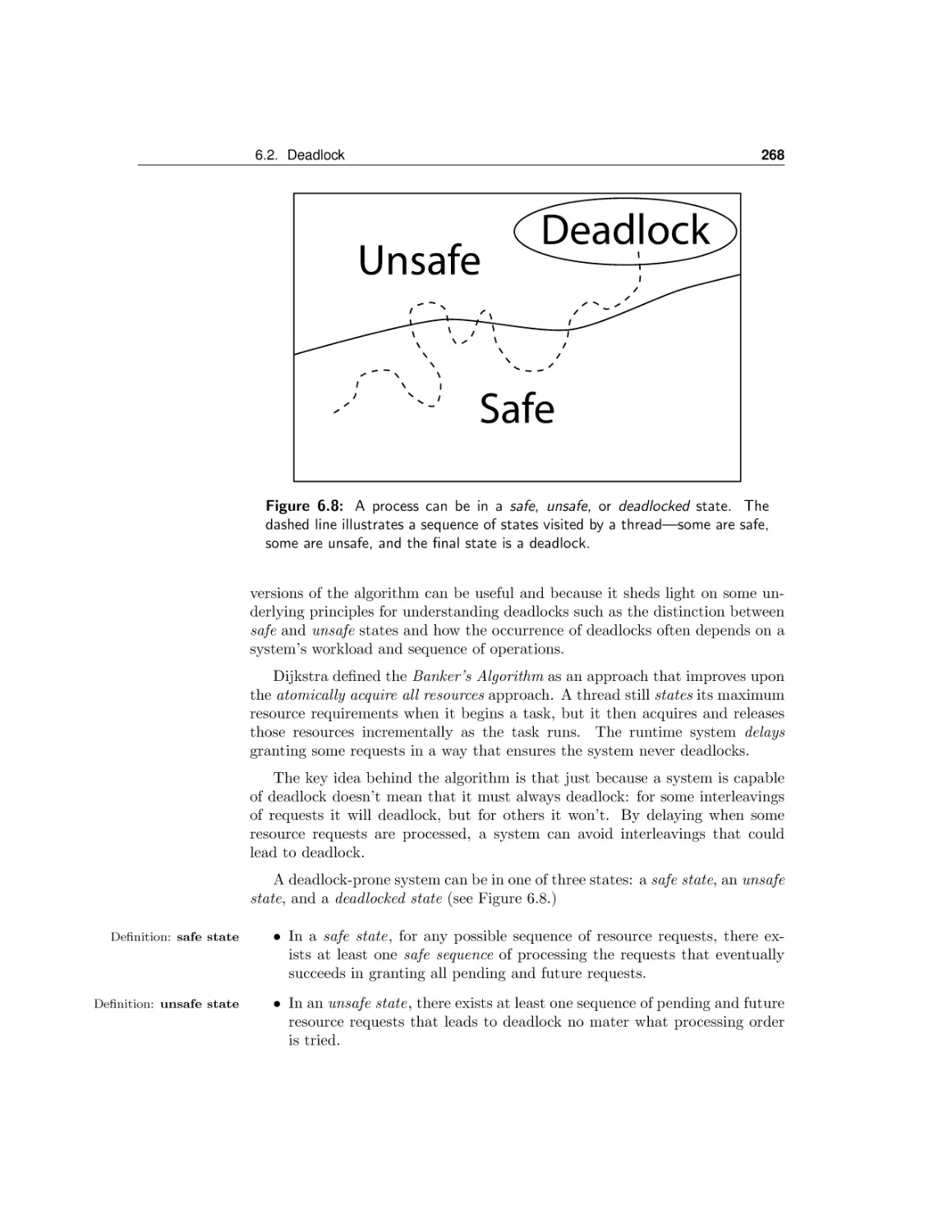
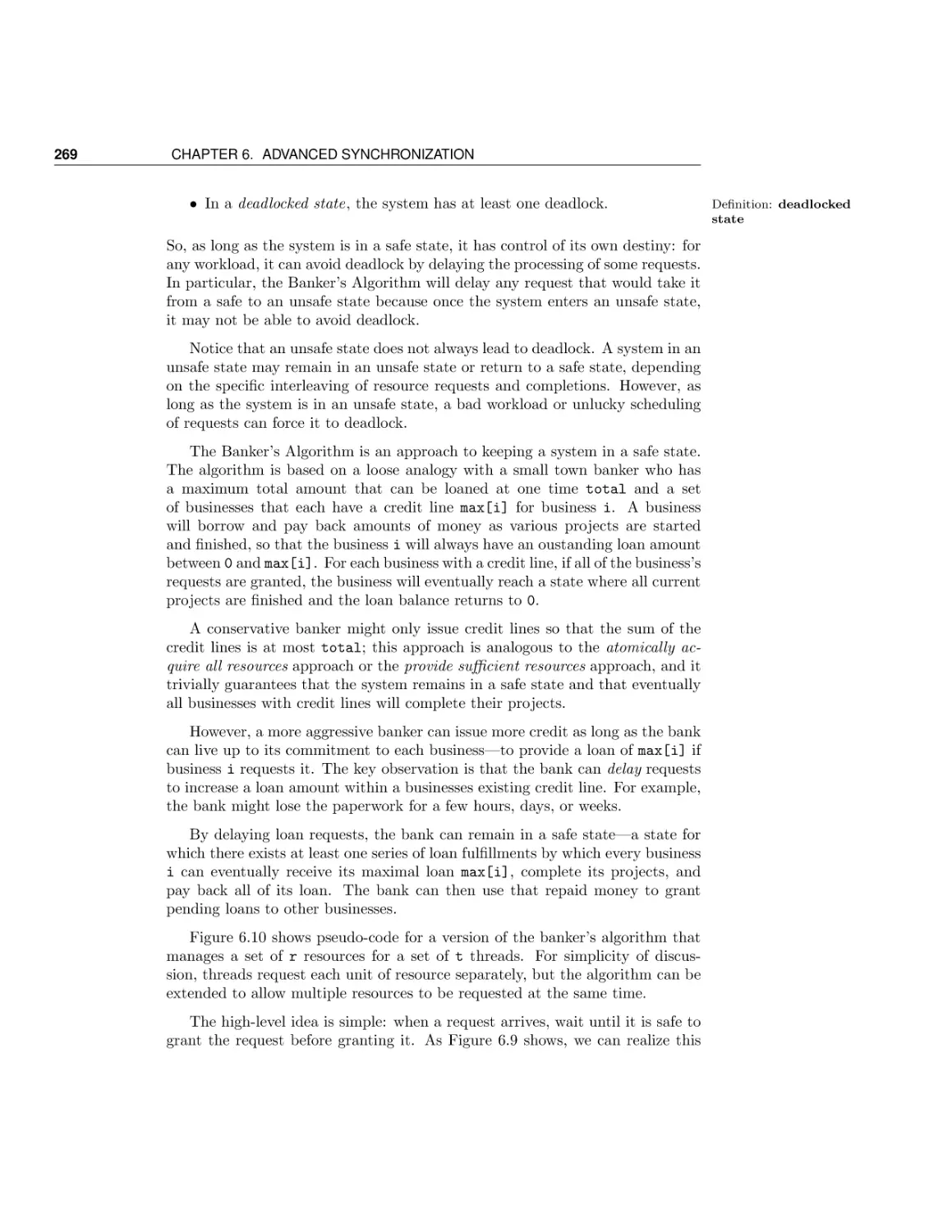
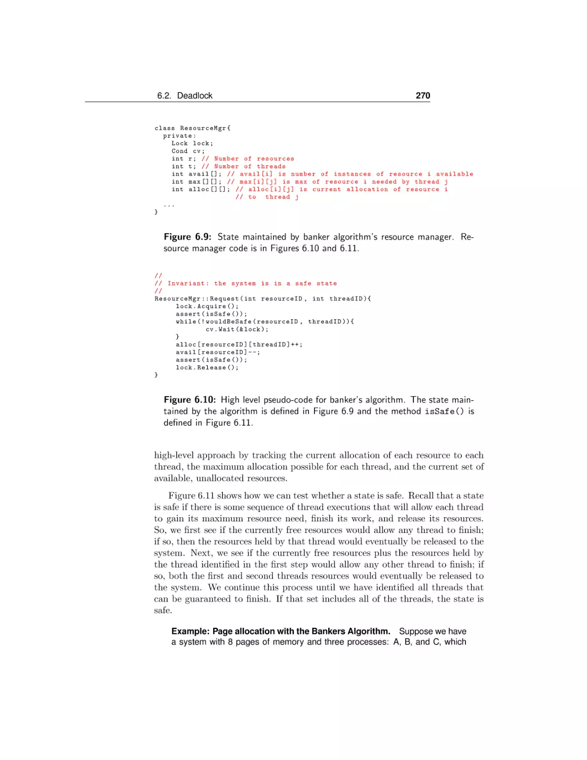
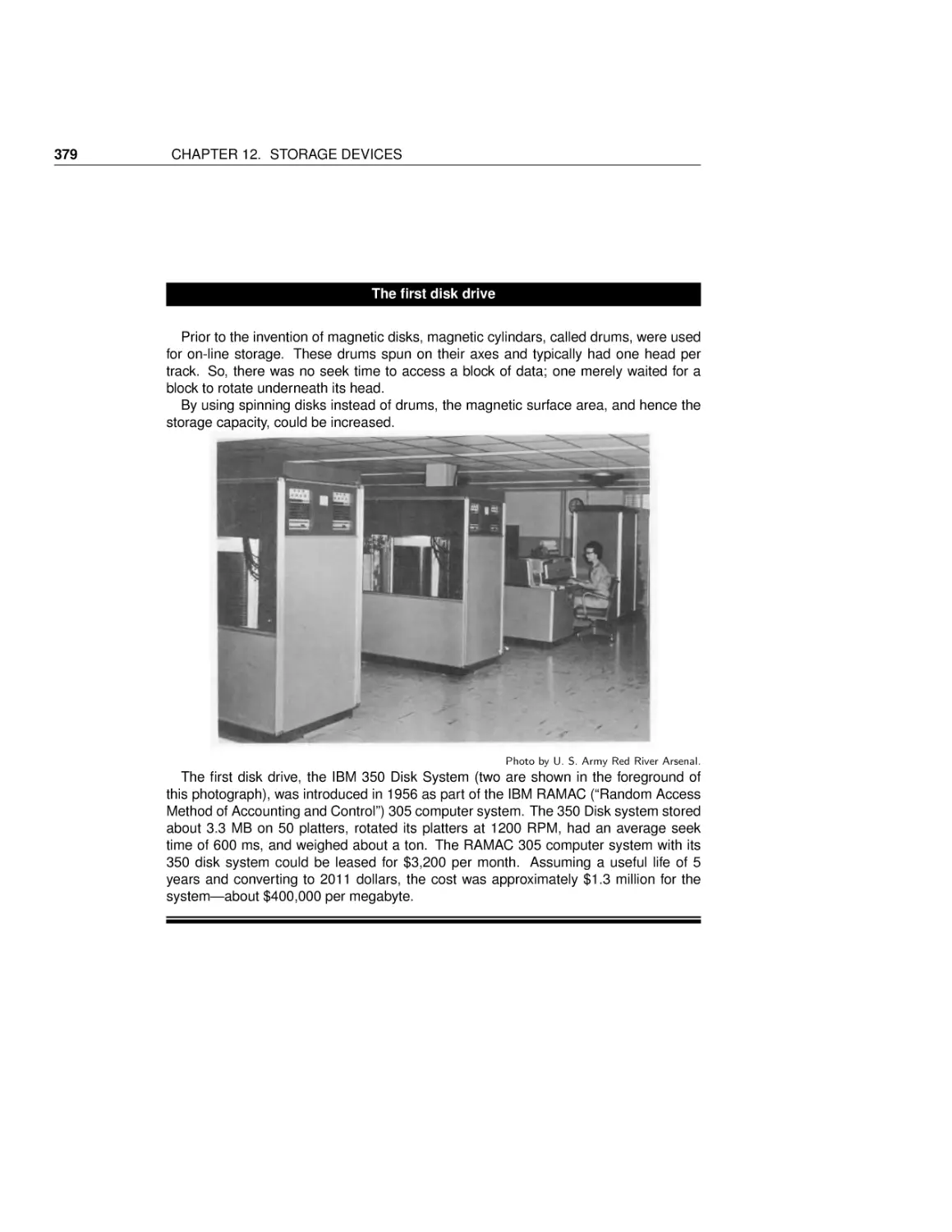
/


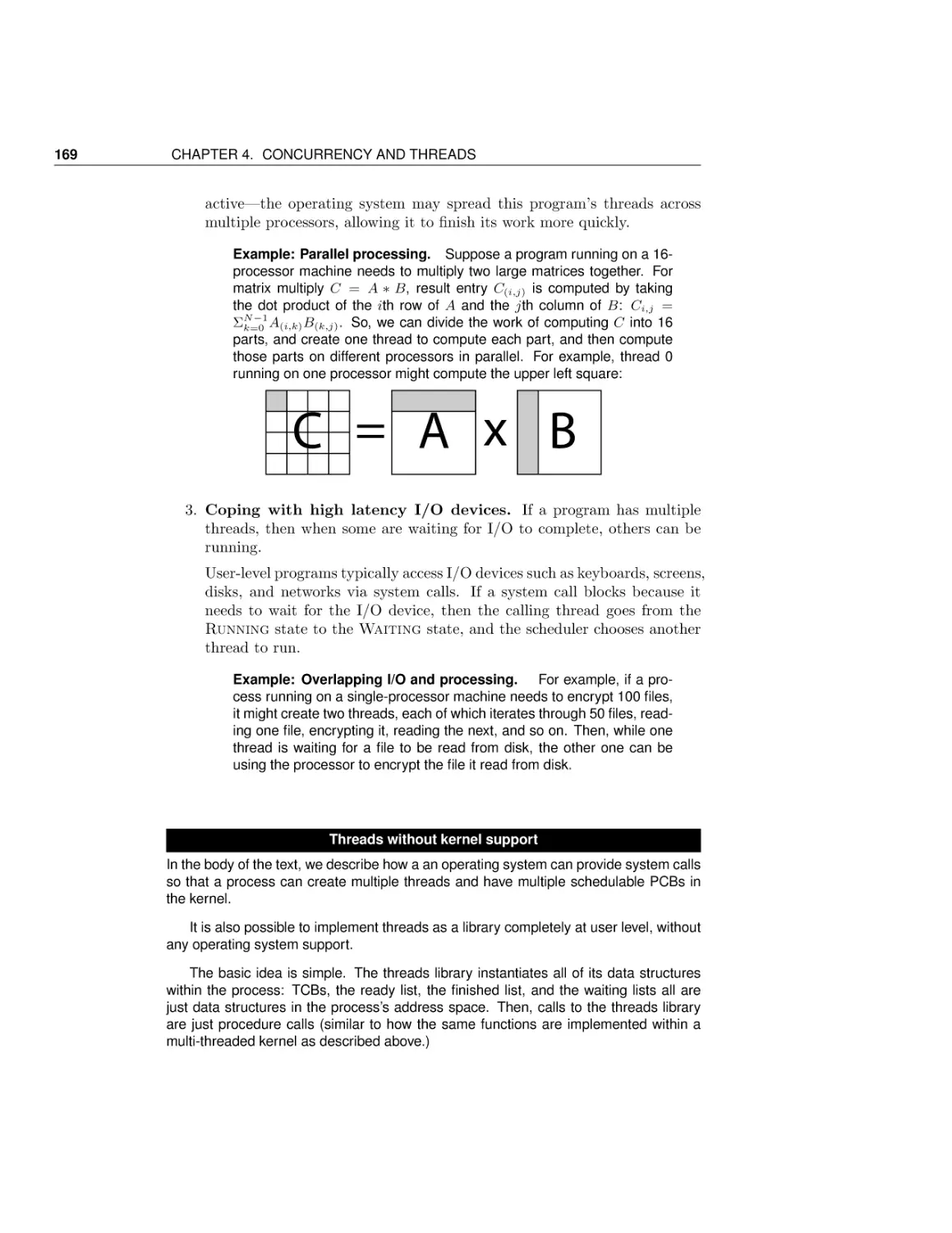


Текст
Operating Systems
Principles and Practice
Anderson and Dahlin
v. 0.22
Operating Systems: Principles and Practice
Version 0.22
Base revision e8814fe, Fri Jan 13 14:51:02 2012 -0600.
Copyright c 2011-2012 by Thomas Anderson and Michael Dahlin, all rights reserved.
Contents
Preface
v
1 Introduction
1
1.1
1.2
1.3
I
What is an operating system?
Evaluation Criteria
A brief history of operating systems
Kernels and Processes
2 The Kernel Abstraction
2.1
2.2
2.3
2.4
2.5
2.6
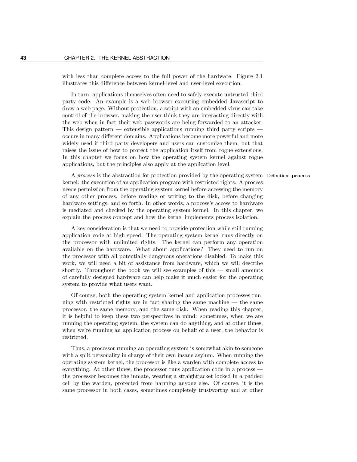
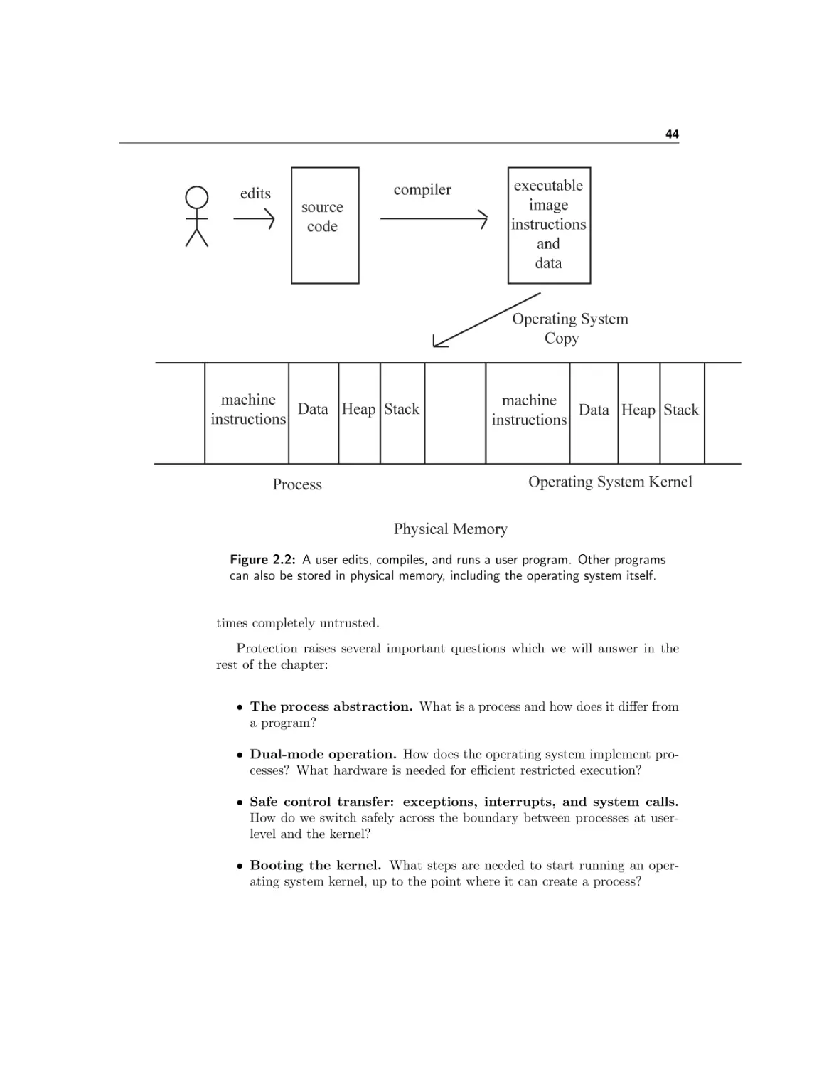
The process concept
Dual-mode operation
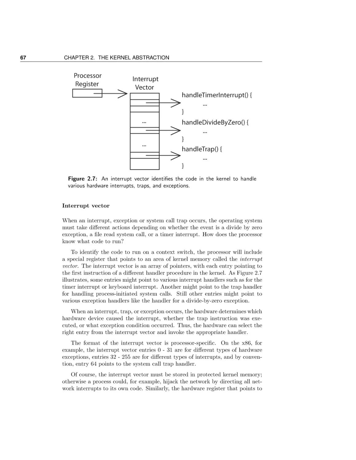
Safe control transfer
Case Study: Booting an operating system kernel
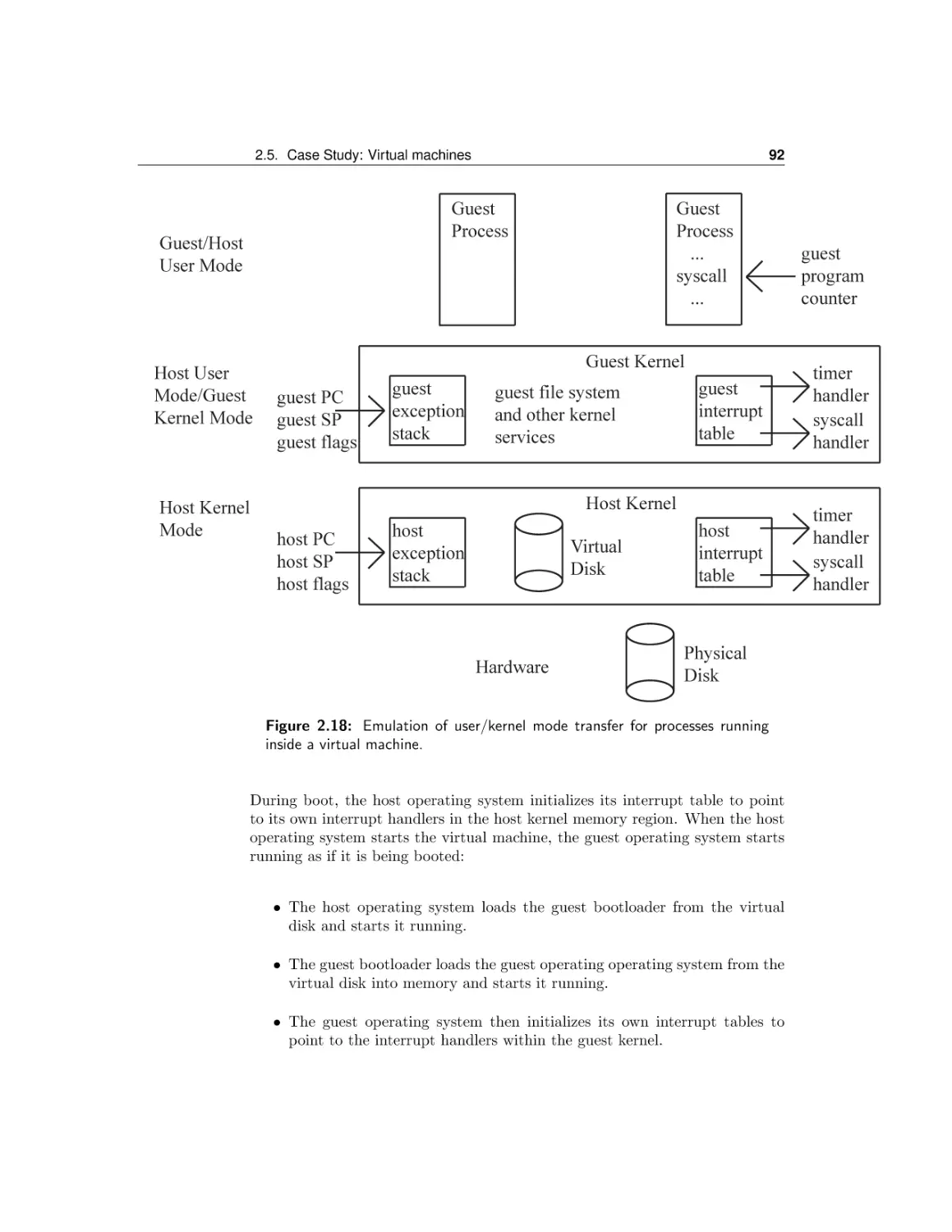
Case Study: Virtual machines
Conclusion and future directions
3 The Programming Interface
3.1
3.2
3.3
3.4
3.5
3.6
II
Process management
Input/output
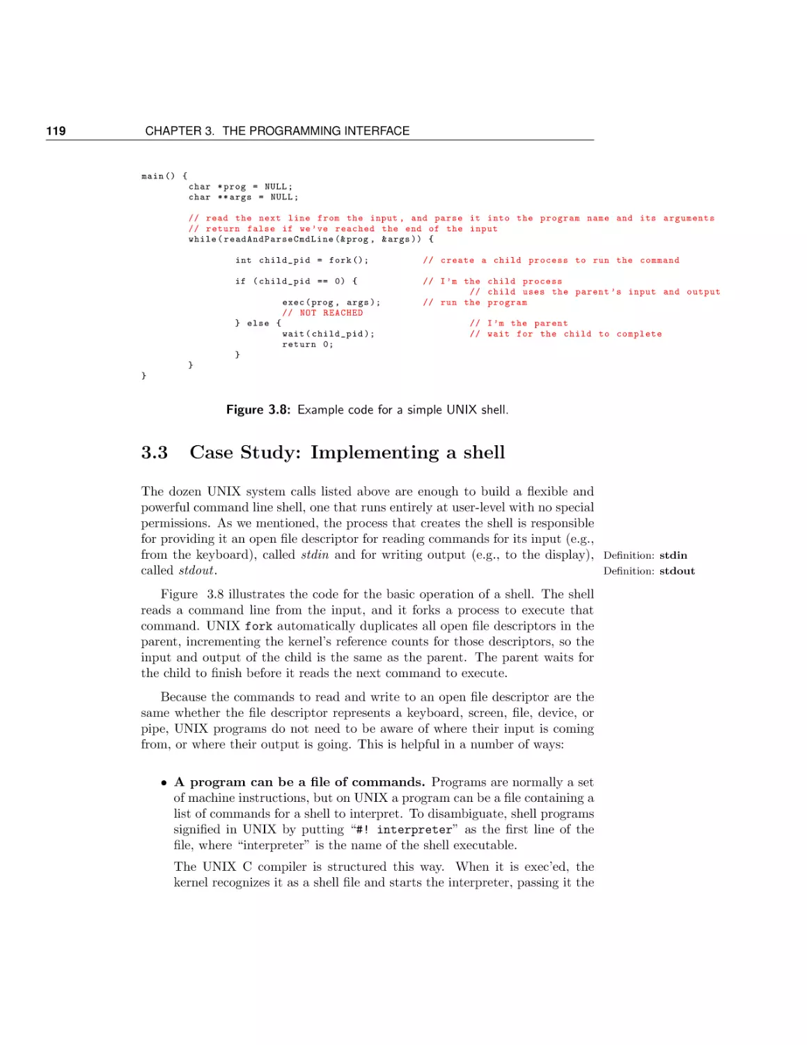
Case Study: Implementing a shell
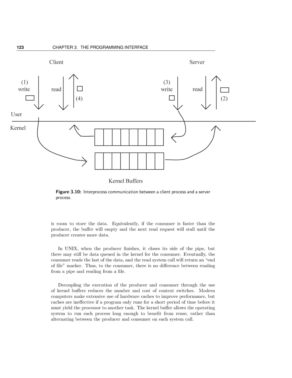
Case Study: Interprocess communication
Operating system structure
Conclusion and future directions
Concurrency
4 Concurrency and Threads
4.1
4.2
4.3
4.4
4.5
Threads: Abstraction and interface
Simple API and example
Thread internals
Implementation details
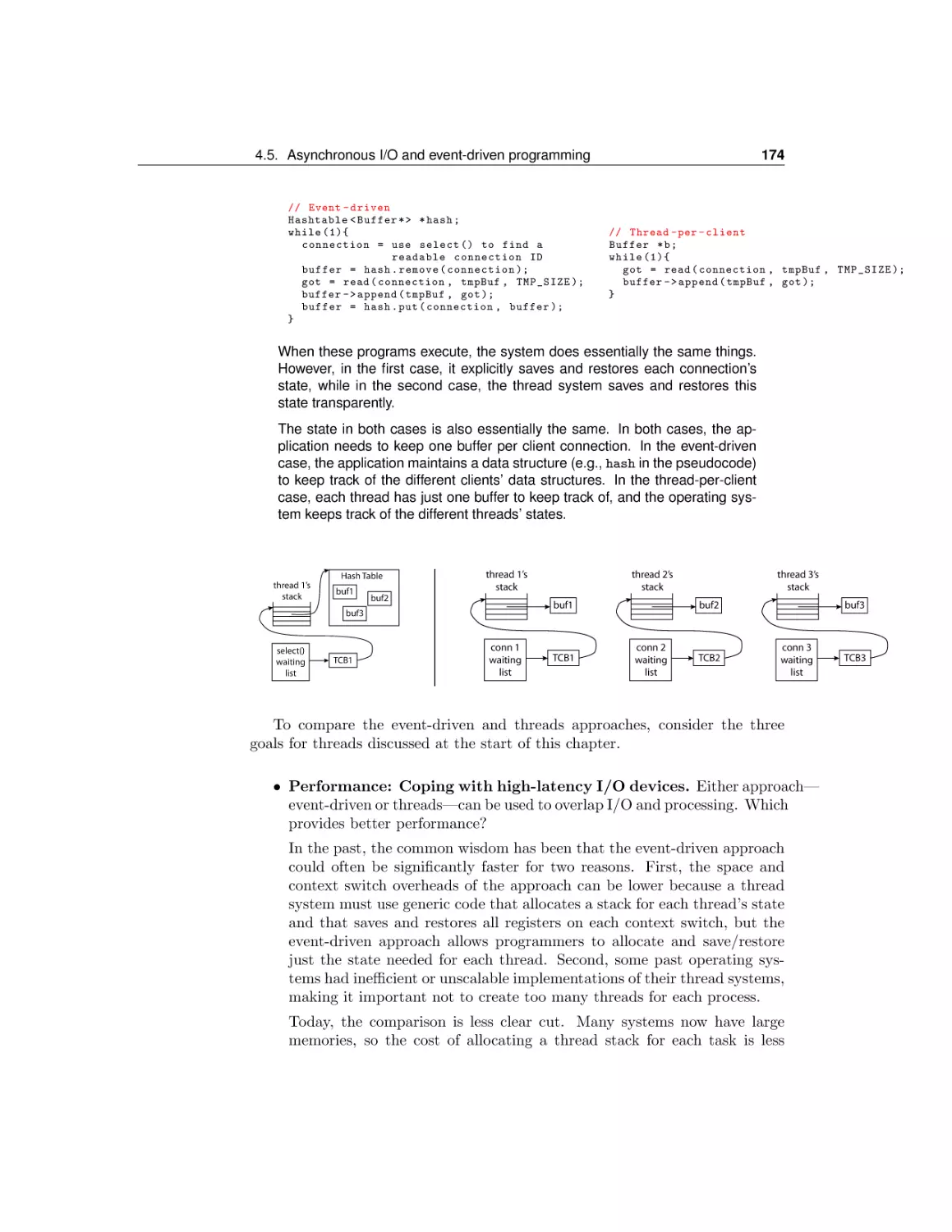
Asynchronous I/O and event-driven programming
4
20
28
39
41
45
47
61
89
91
94
101
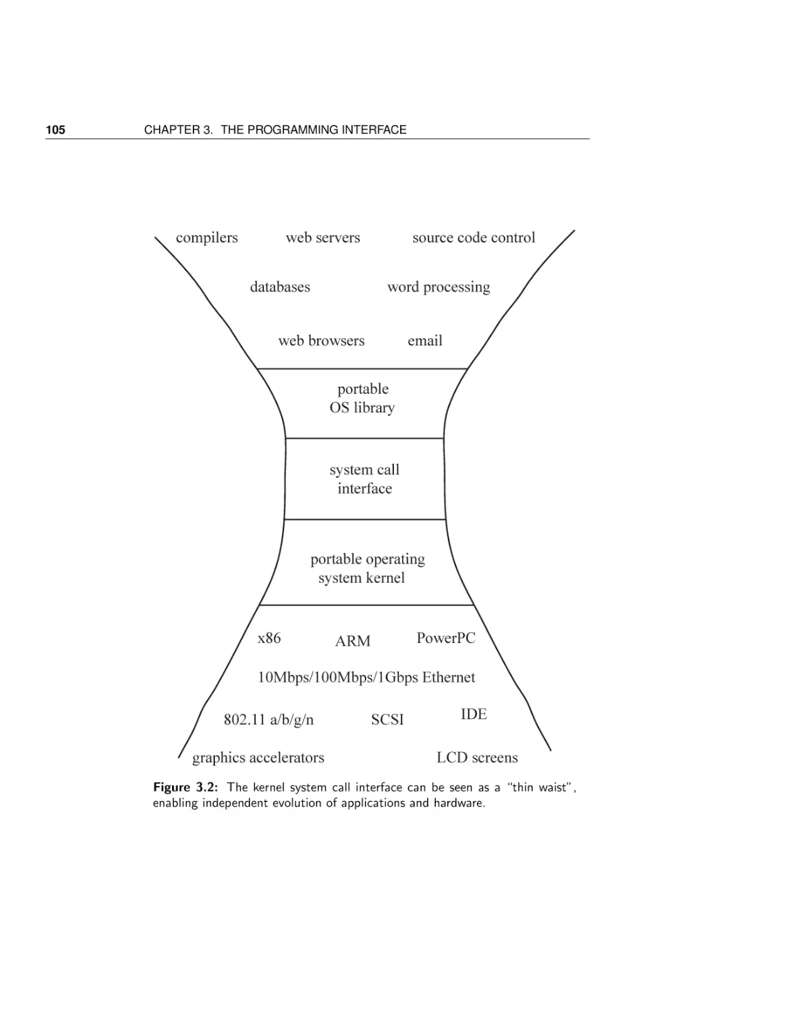
107
114
119
121
124
130
135
137
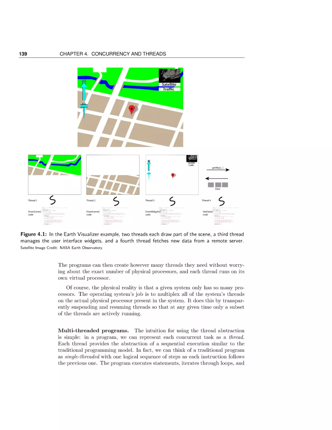
138
145
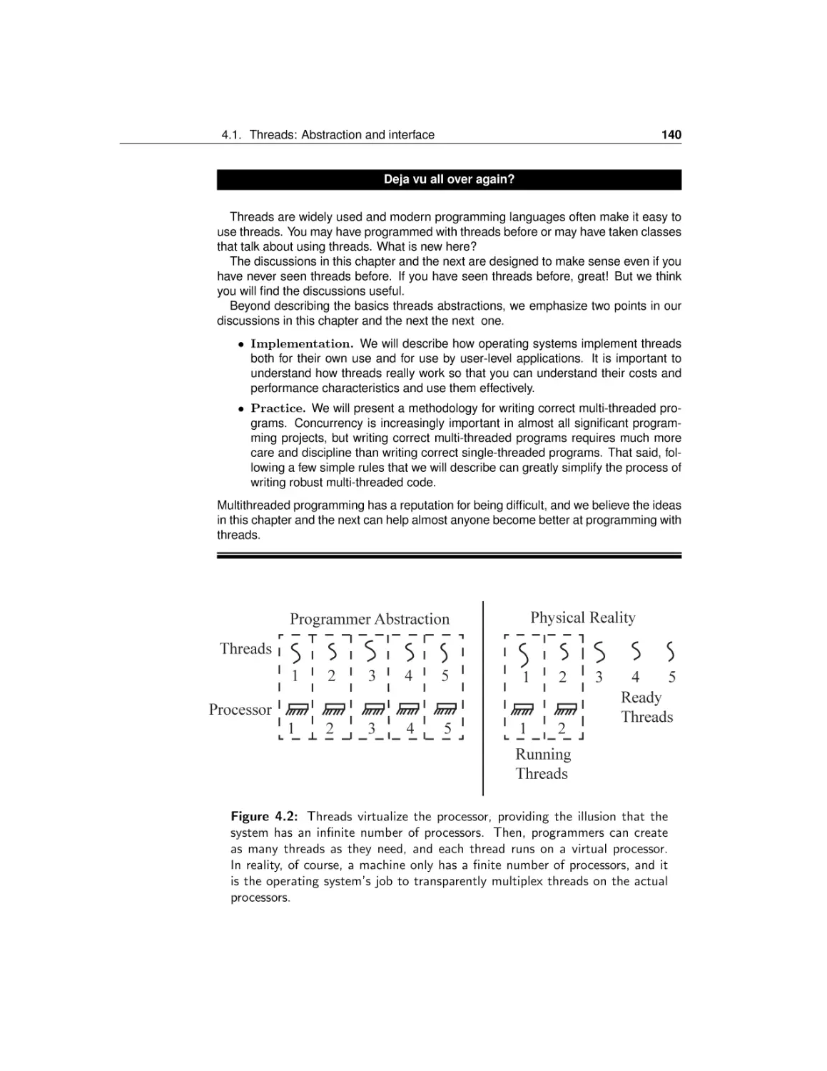
149
155
172
Contents
4.6
Conclusion and future directions
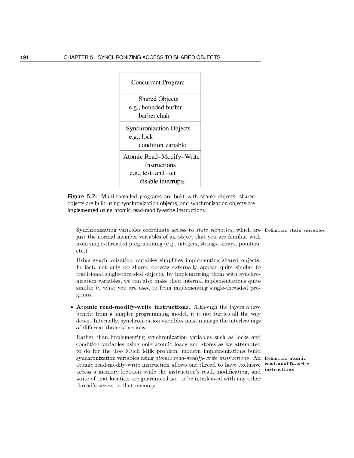
5 Synchronizing Access to Shared Objects
5.1
5.2
5.3
5.4
5.5
5.6
5.7
Challenges
Shared objects and synchronization variables
Lock: Mutual Exclusion
Condition variables: Waiting for a change
Implementing synchronization objects
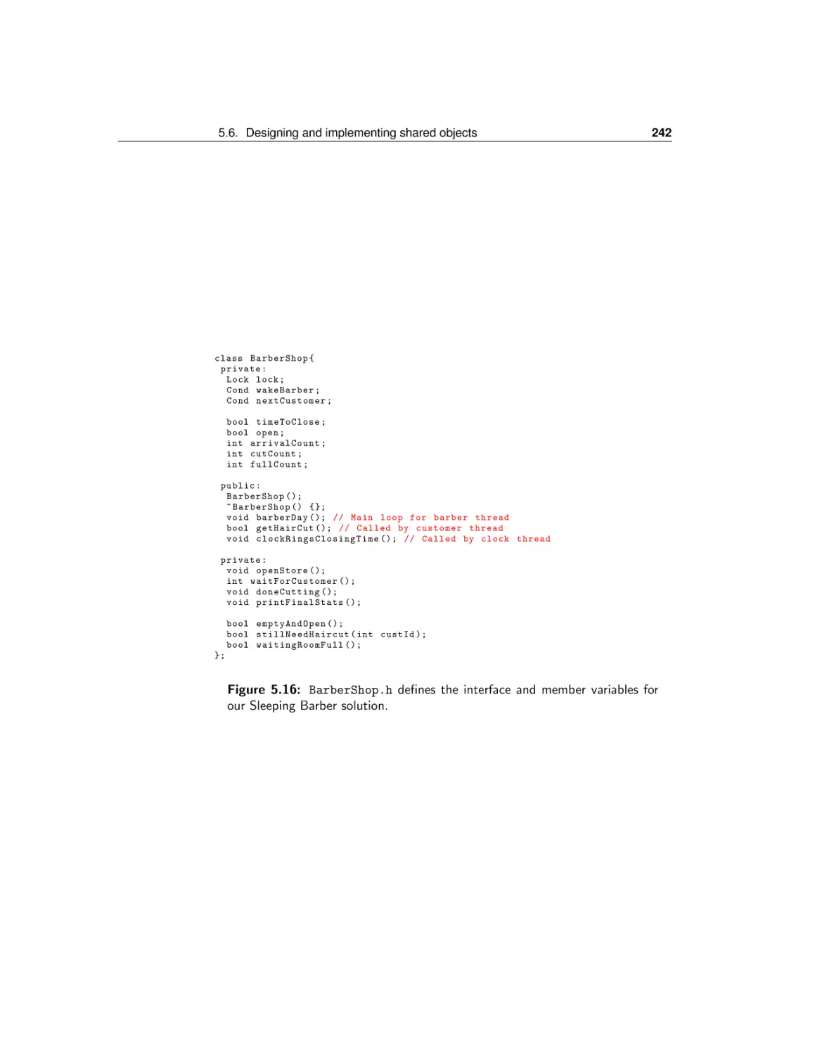
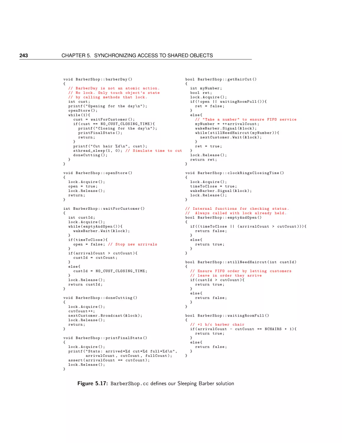
Designing and implementing shared objects
Conclusions
6 Advanced Synchronization
6.1
6.2
6.3
6.4
Multi-object synchronization
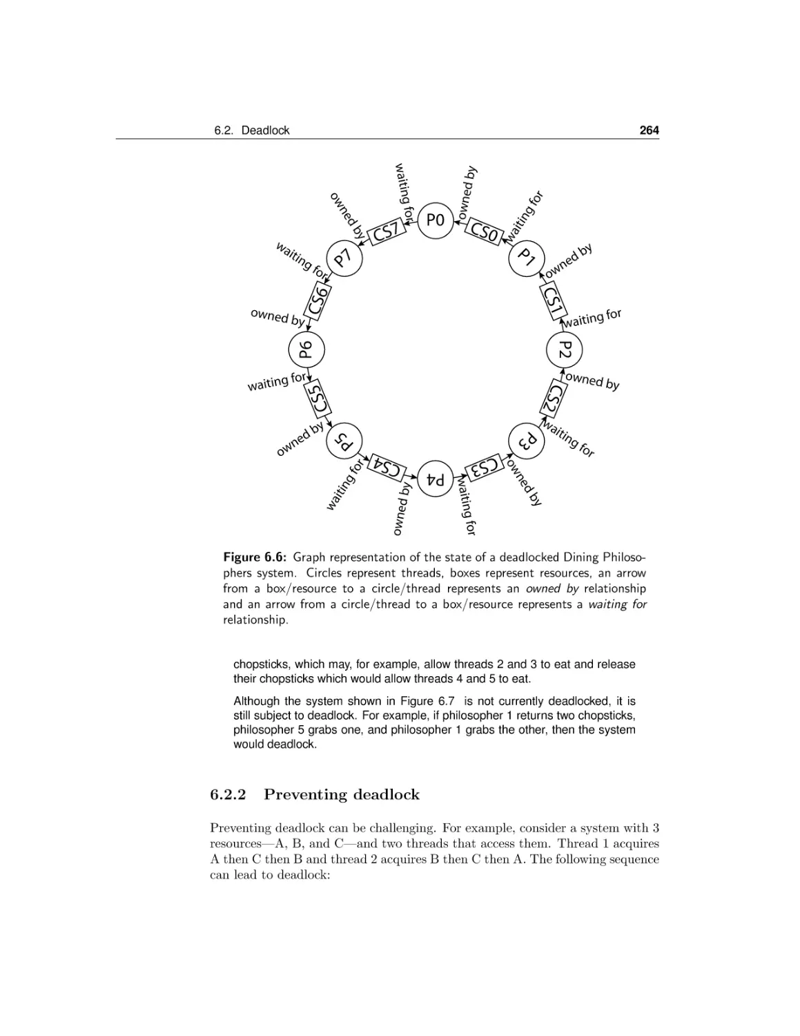
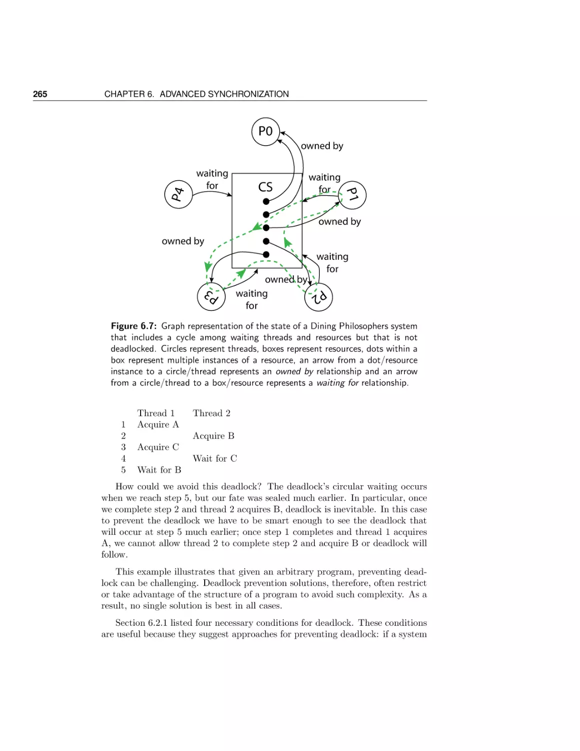
Deadlock
Alternative approaches to synchronization
Conclusion
7 Scheduling
7.1
7.2
7.3
7.4
7.5
7.6
III
Uniprocessor scheduling
Multiprocessor scheduling
Energy-aware scheduling
Real-time scheduling
Queuing theory
Case Study: data center servers
Memory Management
8 Address Translation
8.1
8.2
8.3
8.4
8.5
Address translation concept
Segmentation and Paging
Efficient address translation
Software address translation
Conclusions and future directions
9 Caching and Virtual Memory
9.1
9.2
9.3
9.4
Cache concept: when it works and when it doesn’t
Hardware cache management
Memory mapped files and virtual memory
Conclusions and future directions
10 Applications of Memory Management
10.1
10.2
10.3
10.4
10.5
Zero copy input/output
Copy on write
Process checkpointing
Recoverable memory
Information flow control
ii
175
179
182
189
192
199
212
224
245
251
253
260
278
287
291
294
306
311
312
312
315
317
319
319
320
320
320
320
321
321
322
322
322
323
323
323
323
323
323
iii
CONTENTS
10.6 External pagers
10.7 Virtual machine address translation
10.8 Conclusions and future directions
IV
Persistent Storage
11 File Systems: Introduction and Overview
11.1
11.2
11.3
11.4
The file system abstraction
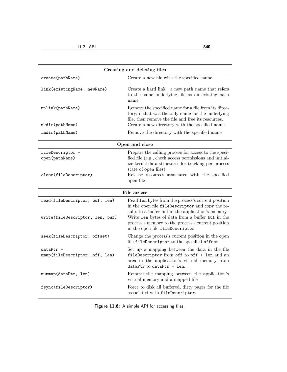
API
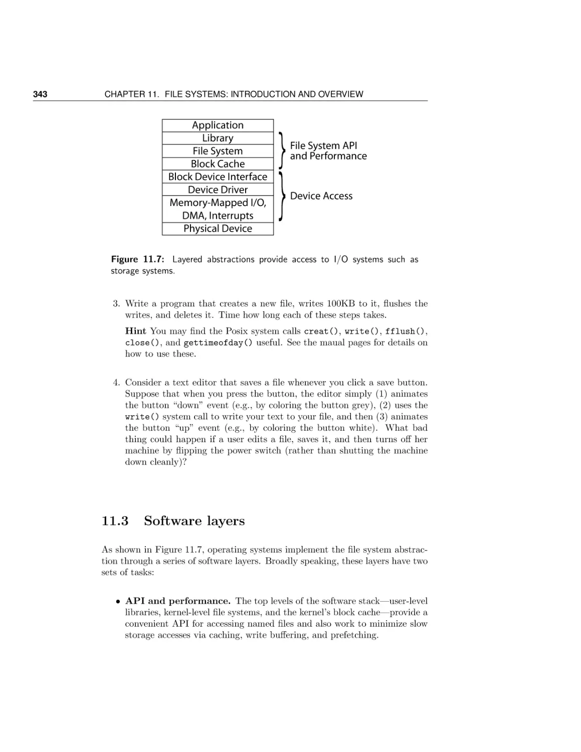
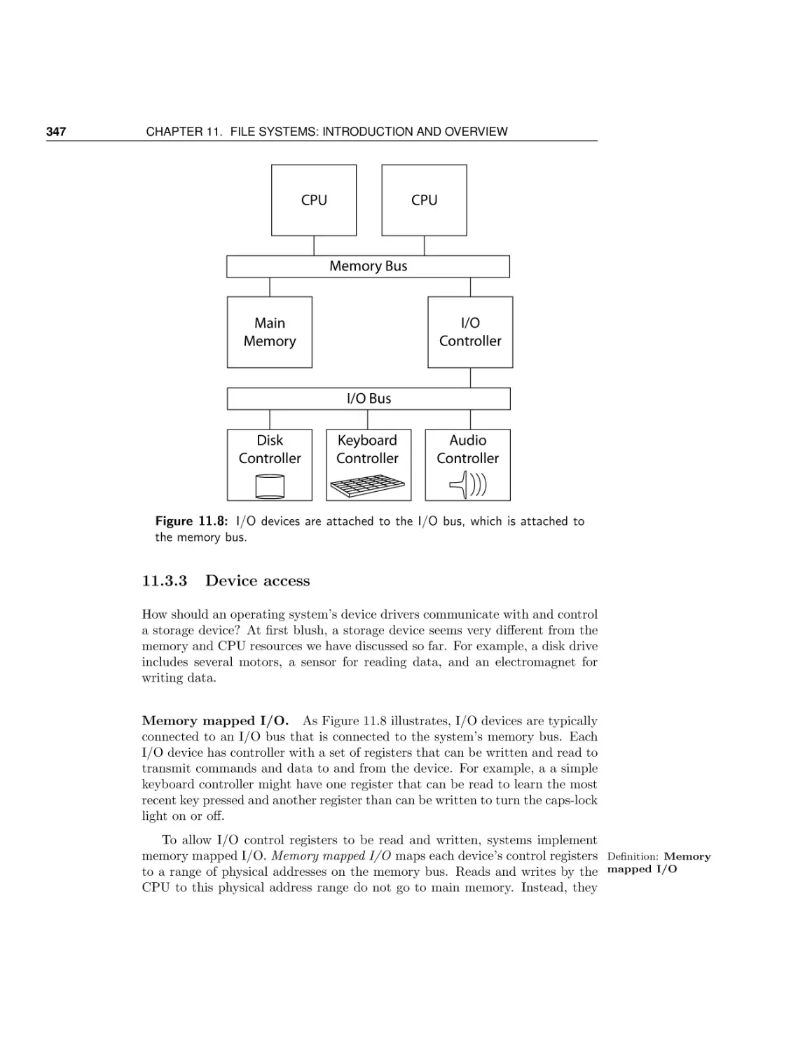
Software layers
Conclusions and future directions
12 Storage Devices
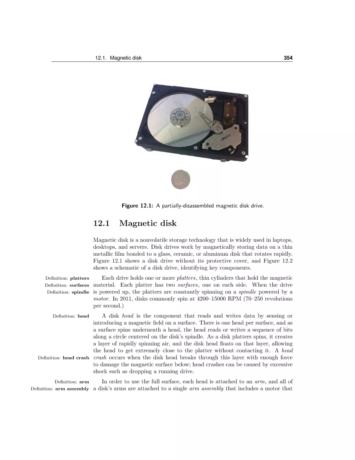
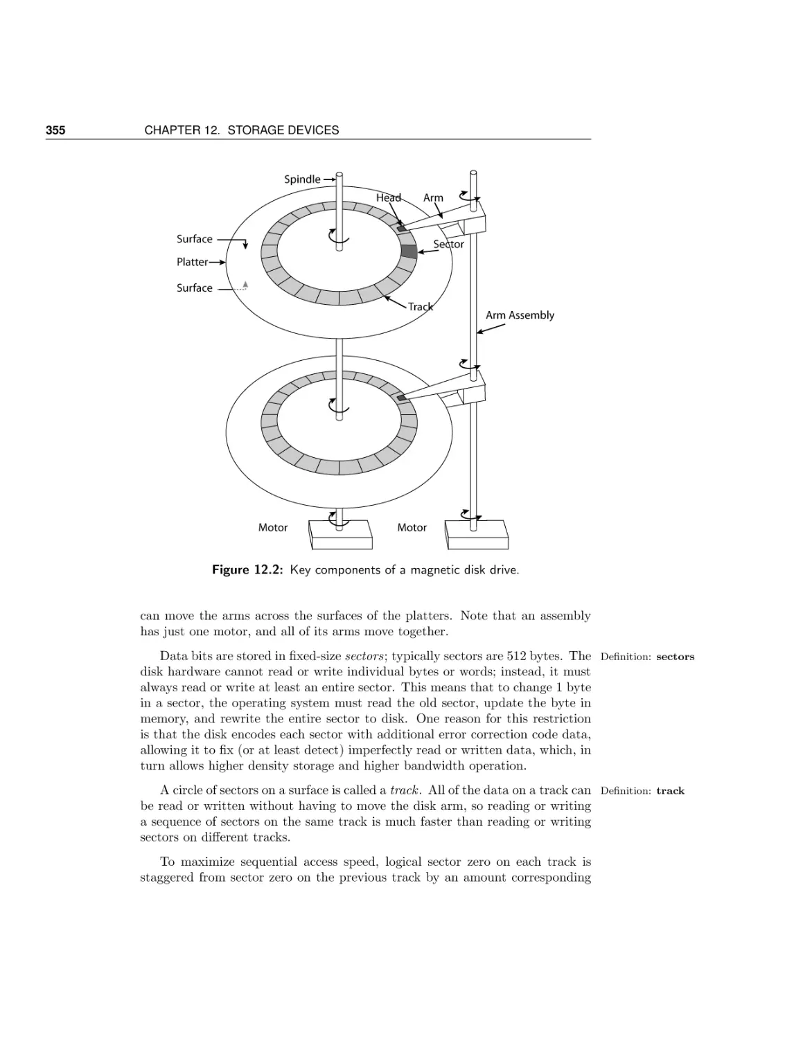
12.1 Magnetic disk
12.2 Flash storage
12.3 Conclusions and future directions
13 Files and Directories
13.1
13.2
13.3
13.4
13.5
Accessing files: API and caching
Files: Placing and finding data
Directories: Naming data
Putting it all together: File access in FFS
Alternatives to file systems
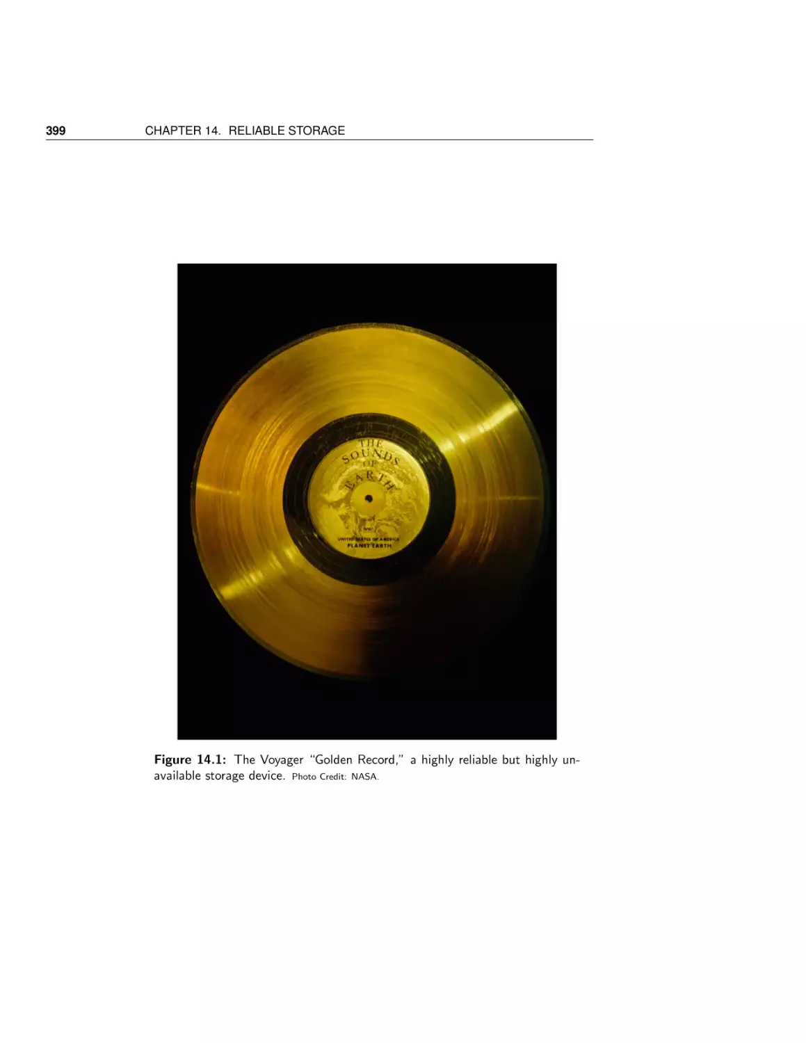
14 Reliable Storage
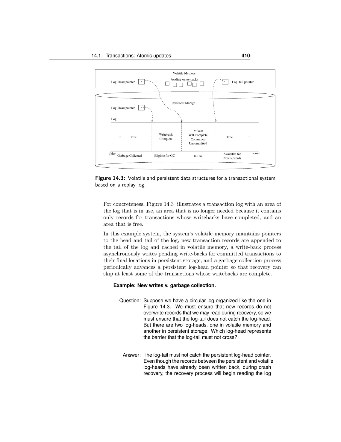
14.1 Transactions: Atomic updates
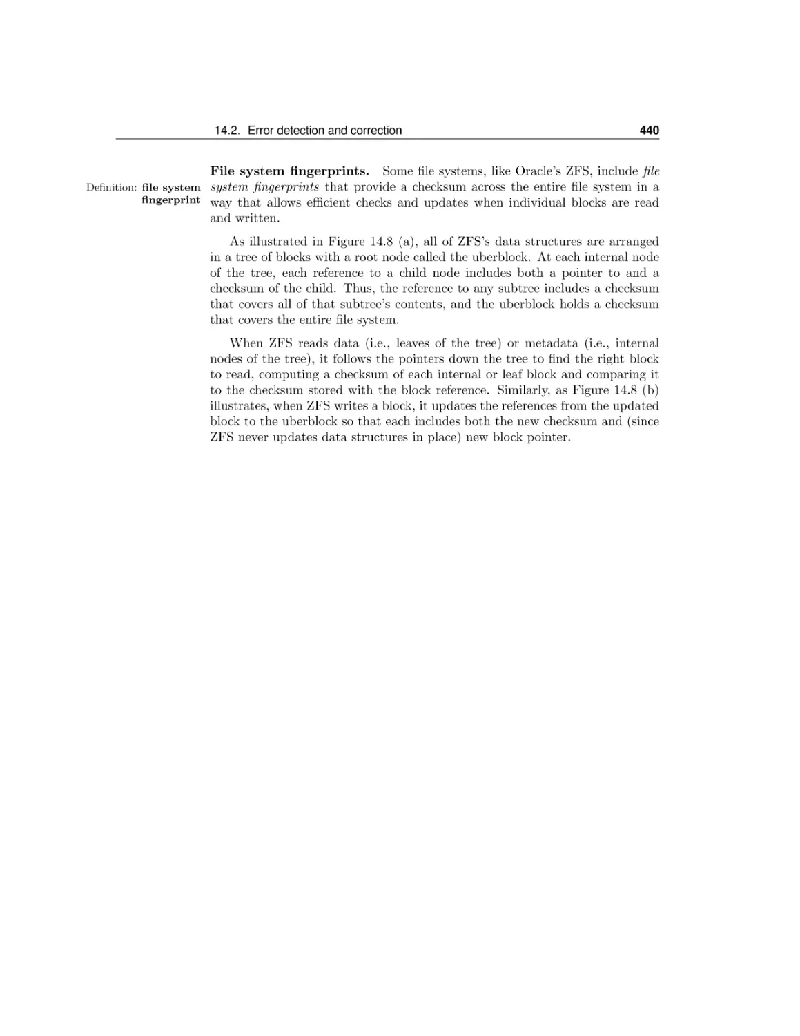
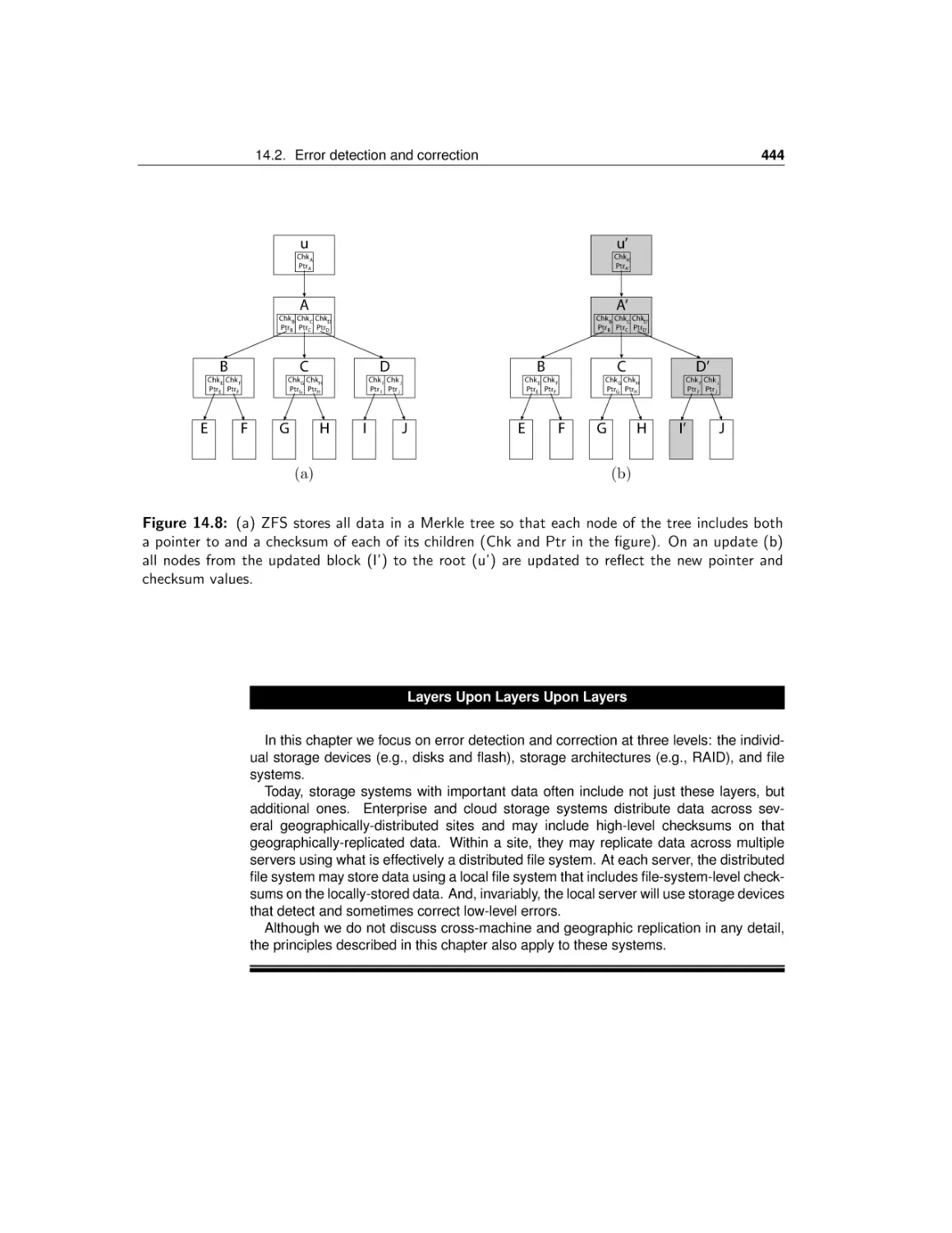
14.2 Error detection and correction
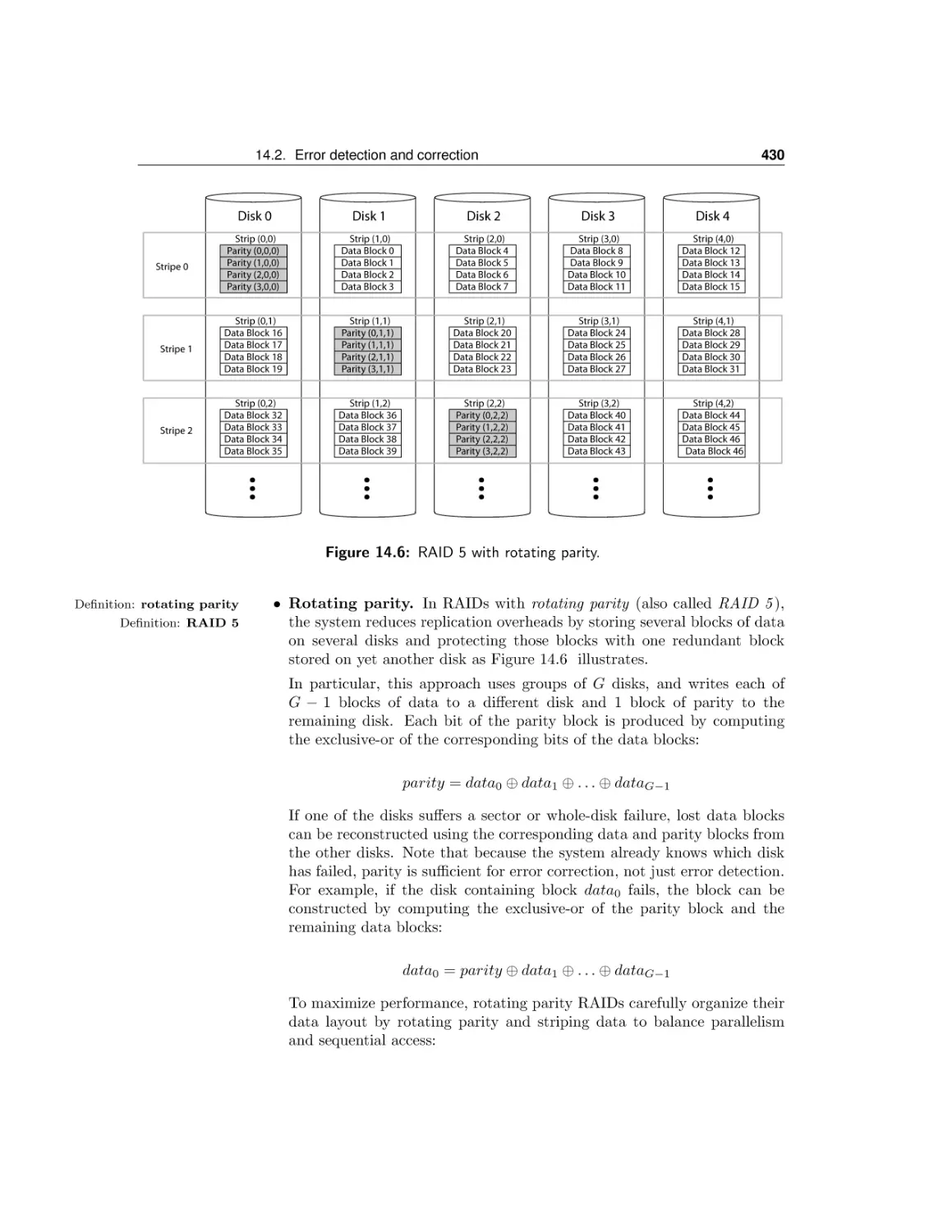
14.3 Conclusion and future directions
V
Index
Index
323
324
324
325
327
332
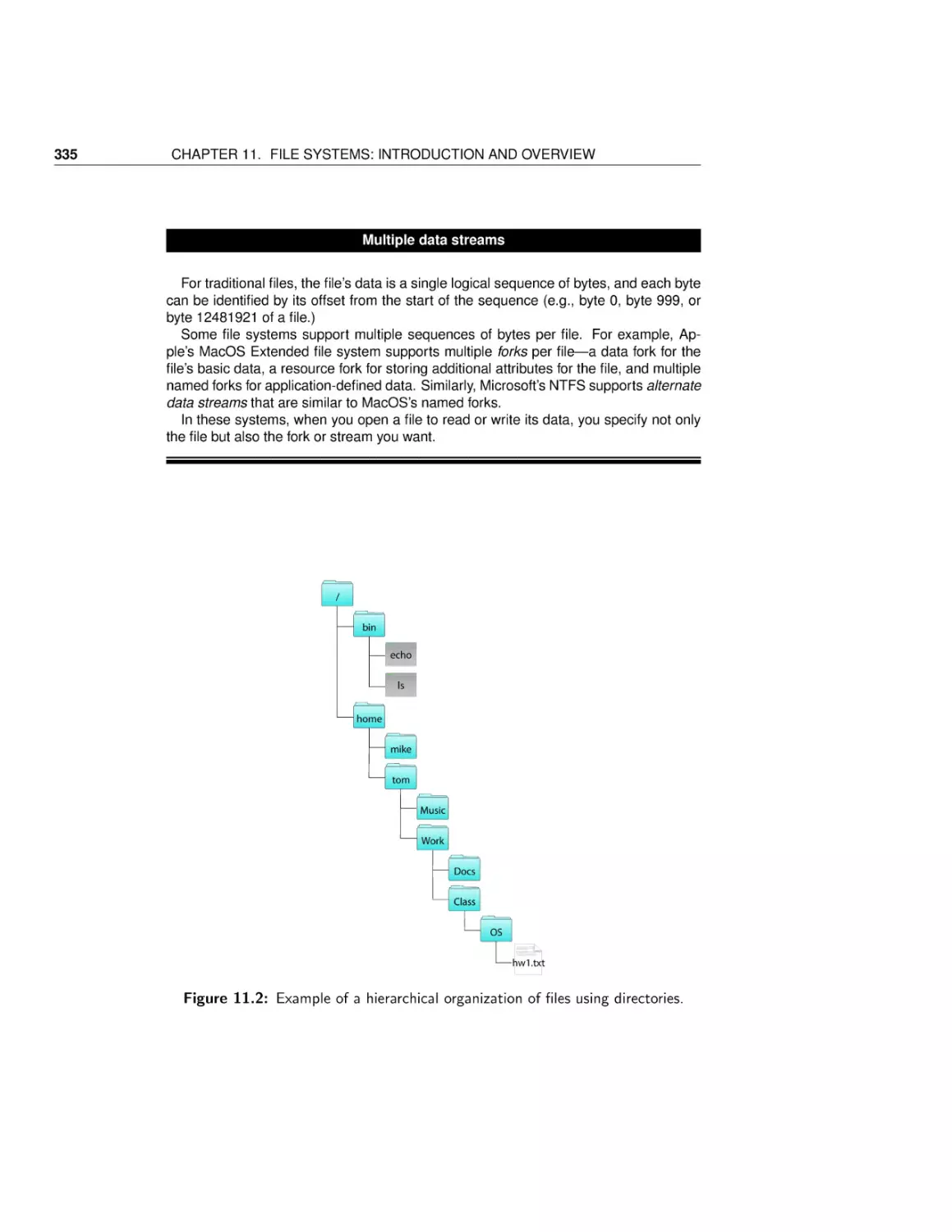
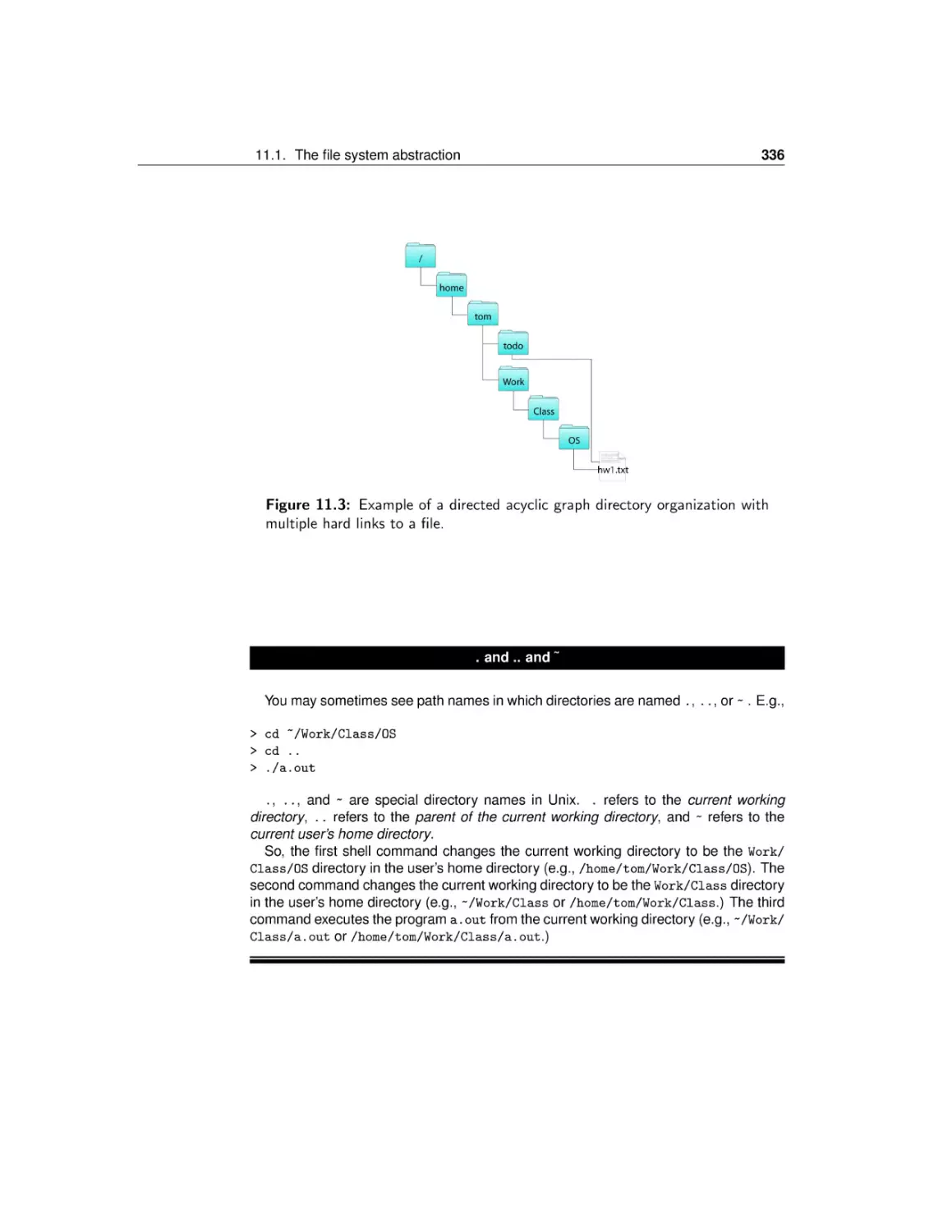
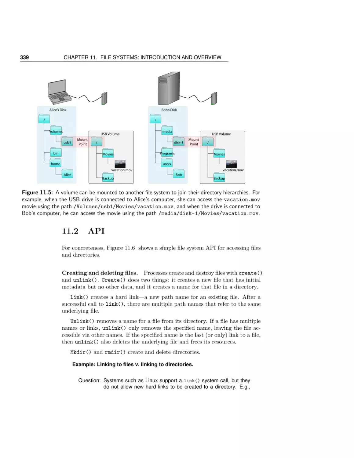
339
343
351
353
354
369
376
385
386
388
393
394
394
397
401
421
447
453
455
Contents
iv
Preface
Why We’re Writing This Book
There has been a huge amount of innovation in both the principles and practice
of operating systems over the past two decades. The pace of innovation in
operating systems has, if anything, increased over the past few years, with the
introduction of the iOS and Android operating systems for smartphones, the
shift to multicore computers, and the advent of cloud computing.
Yet many operating systems textbooks treat the field as if it is static — that
almost everything we need to cover in our classes was invented in the 60’s and
70’s. No! We strongly believe that students both need to, and can, understand
modern operating systems concepts and modern implementation techniques.
At Texas and Washington, we have been teaching the topics covered in this
textbook for years, winning awards for our teaching. The approach in this
book is the same one we use in organizing our own courses: that it is essential
for students to learn both principles and practice, that is, both concepts and
implementation, rather than either alone.
Although this book focuses on operating systems, we believe the concepts
and principles are important for anyone getting a degree in computer science or
computer engineering. The core ideas in operating systems — protection, concurrency, virtualization, resource allocation, and reliable storage — are widely
used throughout computer science. Anyone trying to build resilient, secure,
flexible computer systems needs to have a deep grounding in these topics and
to be able to apply these concepts in a variety of settings. This is especially
true in a modern world where nearly everything a user does is distributed, and
nearly every computer is multi-core. Operating systems concepts are popping
up in many different areas; even web browsers and cloud computing platforms
have become mini-operating systems in their own right.
Precisely because operating systems concepts are among the most difficult
in all of computer science, it is also important to ground students in how these
ideas are applied in practice in real operating systems of today. In this book, we
give students both concepts and working code. We have designed the book to
support and be complemented with a rigorous operating systems course project,
v
Contents
vi
such as Nachos, Pintos, JOS, or Linux. Our treatment, however, is general —
it is not our intent to completely explain any particular operating system or
course project.
Because the concepts in this textbook are so fundamental to much of the
practice of modern computer science, we believe a rigorous operating systems
course should be taken early in an undergraduate’s course of study. For many
students, an operating systems class is the ticket to an internship and eventually to a full-time position. We have designed this textbook assuming only
that students have taken a class on data structures and one on basic machine
structures. In particular, we have designed our book to interface well if students
have used the Bryant and O’Halloran textbook on machine structures. Since
some schools only get through the first half of Bryant and O’Halloran in their
machine structures course, our textbook reviews and covers in much more depth
the material from the second half of that book.
An Overview of the Content
The textbook is organized to allow each instructor to choose an appropriate
level of depth for each topic. Each chapter begins at a conceptual level, with
implementation details and the more advanced material towards the end. A
more conceptual course will skip the back parts of several of the chapters; a
more advanced or more implementation-oriented course will need to go into
chapters in more depth. No single semester course is likely to be able to cover
every topic we have included, but we think it is a good thing for students to
come away from an operating systems course with an appreciation that there is
still a lot for them to learn.
Because students learn more by needing to solve problems, we have integrated some homework questions into the body of each chapter, to provide
students a way of judging whether they understood the material covered to
that point. A more complete set of sample assignments is given at the end of
each chapter.
The book is divided into five parts: an introduction (Chapter 1), kernels and
processes (Chapters 2-3), concurrency, synchronization and scheduling (Chapters 4-7), memory management (Chapters 8-10), and persistent storage (Chapters 11-13).
The goal of chapter 1 is to introduce the recurring themes found in the later
chapters. We define some common terms, and we provide a bit of the history
of the development of operating systems.
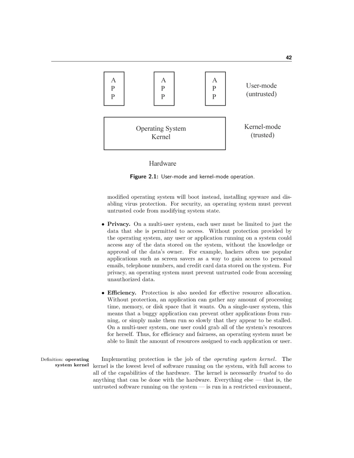
Chapter 2 covers kernel-based process protection — the concept and implementation of executing a user program with restricted privileges. The concept
of protected execution and safe transfer across privilege levels is a key concept
to most modern computer systems, given the increasing salience of computer
security issues. For a quick introduction to the concepts, students need only
vii
CONTENTS
read through 2.3.2; the chapter then dives into the mechanics of system calls,
exceptions and interrupts in some detail. Some instructors launch directly into
concurrency, and cover kernels and kernel protection afterwards, as a lead-in to
address spaces and virtual memory. While our textbook can be used that way,
we have found that students benefit from a basic understanding of the role of
operating systems in executing user programs, before introducing concurrency.
Chapter 3 is intended as an impedance match for students of differing backgrounds. Depending on student background, it can be skipped or covered in
depth. The chapter covers the operating system from a programmer’s perspective: process creation and management, device-independent input/output,
interprocess communication, and network sockets. Our goal is that students be
able to understand at a detailed level what happens between a user clicking on
a link in a web browser, and that request being transferred through the operating system kernel on each machine to the web server running at user-level,
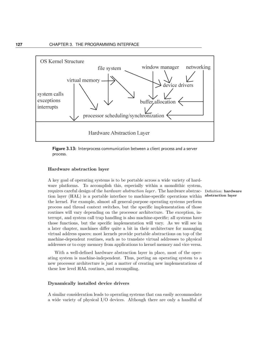
and back again. The second half of Chapter 3 dives into the organization of the
operating system itself — how device drivers and the hardware abstraction layer
work in a modern operating system; the difference between a monolithic and a
microkernel operating system; and how policy and mechanism can be separated
in modern operating systems.
Chapter 4 motivates and explains the concept of threads. Because of the
increasing importance of concurrent programming, and its integration with Java,
many students will have been introduced to multi-threaded programming in
an earlier class. This is a bit dangerous, as testing will not expose students
to the errors they are making in concurrent programming. Thus, the goal of
this chapter is to provide a solid conceptual framework for understanding the
semantics of concurrency, as well as how concurrent threads are implemented in
both the operating system kernel and in user-level libraries. Instructors needing
to go more quickly can omit Section 3.4 and 3.5.
Chapter 5 discusses the synchronization of multi-threaded programs, a central part of all operating systems and increasingly important in many other
contexts. Our approach is to describe one effective method for structuring
concurrent programs (monitors), rather than to cover in depth every proposed
mechanism. In our view, it is important for students to master one methodology,
and monitors are a particularly robust and simple one, capable of implementing most concurrent programs efficiently. Implementation of synchronization
primitives are covered in Section 5.5; this can be skipped without compromising
student understanding.
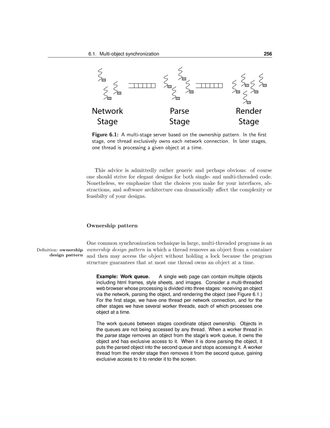
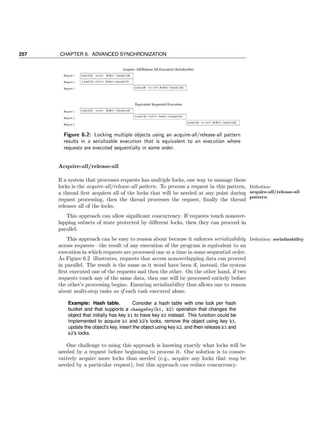
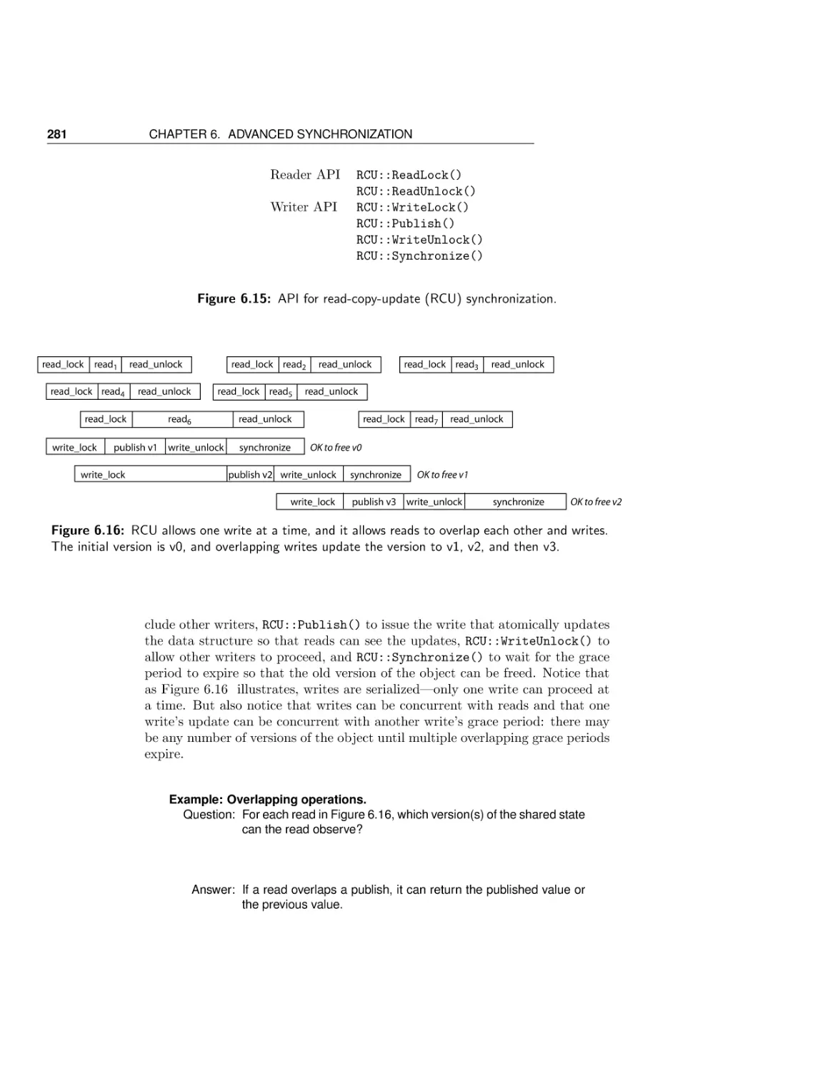
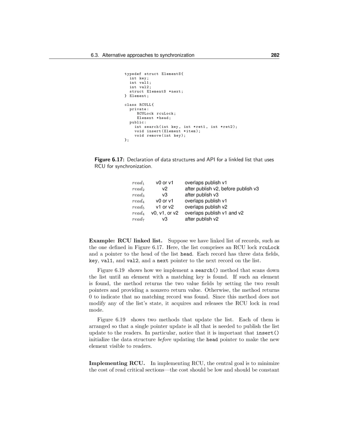
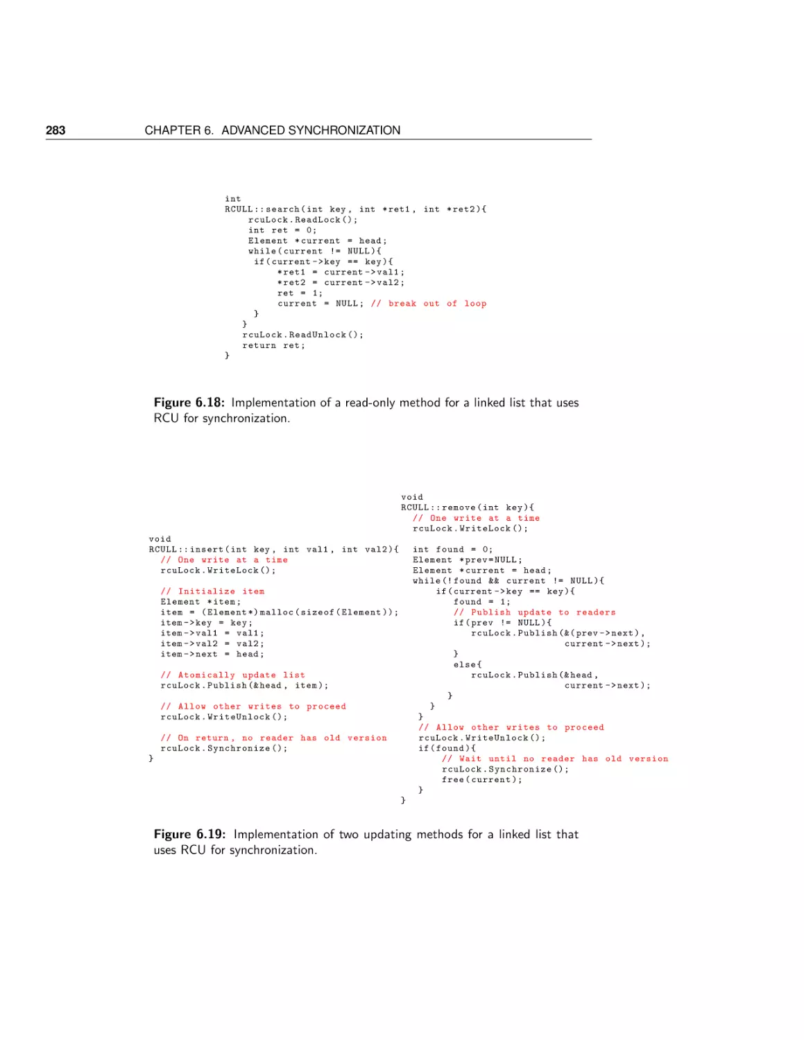
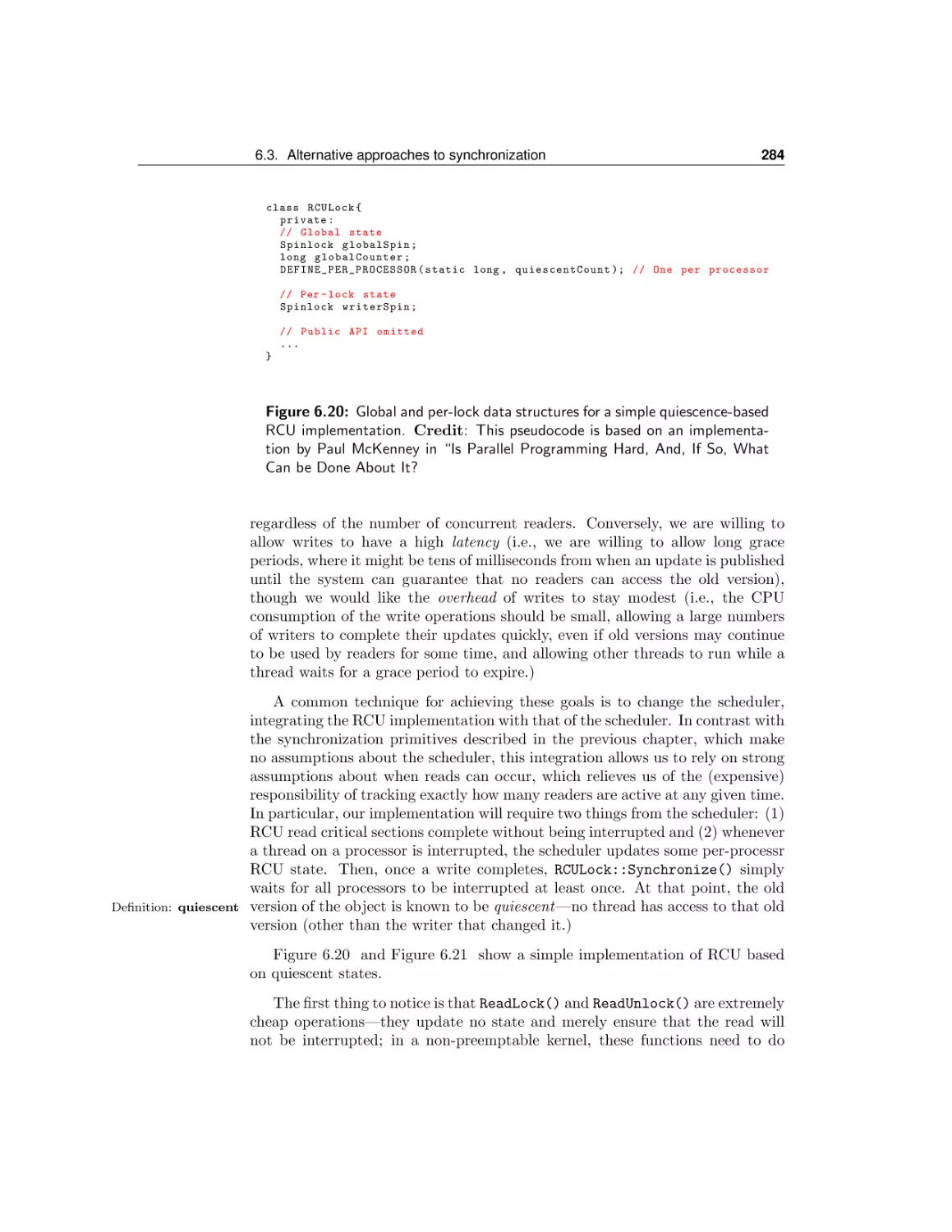
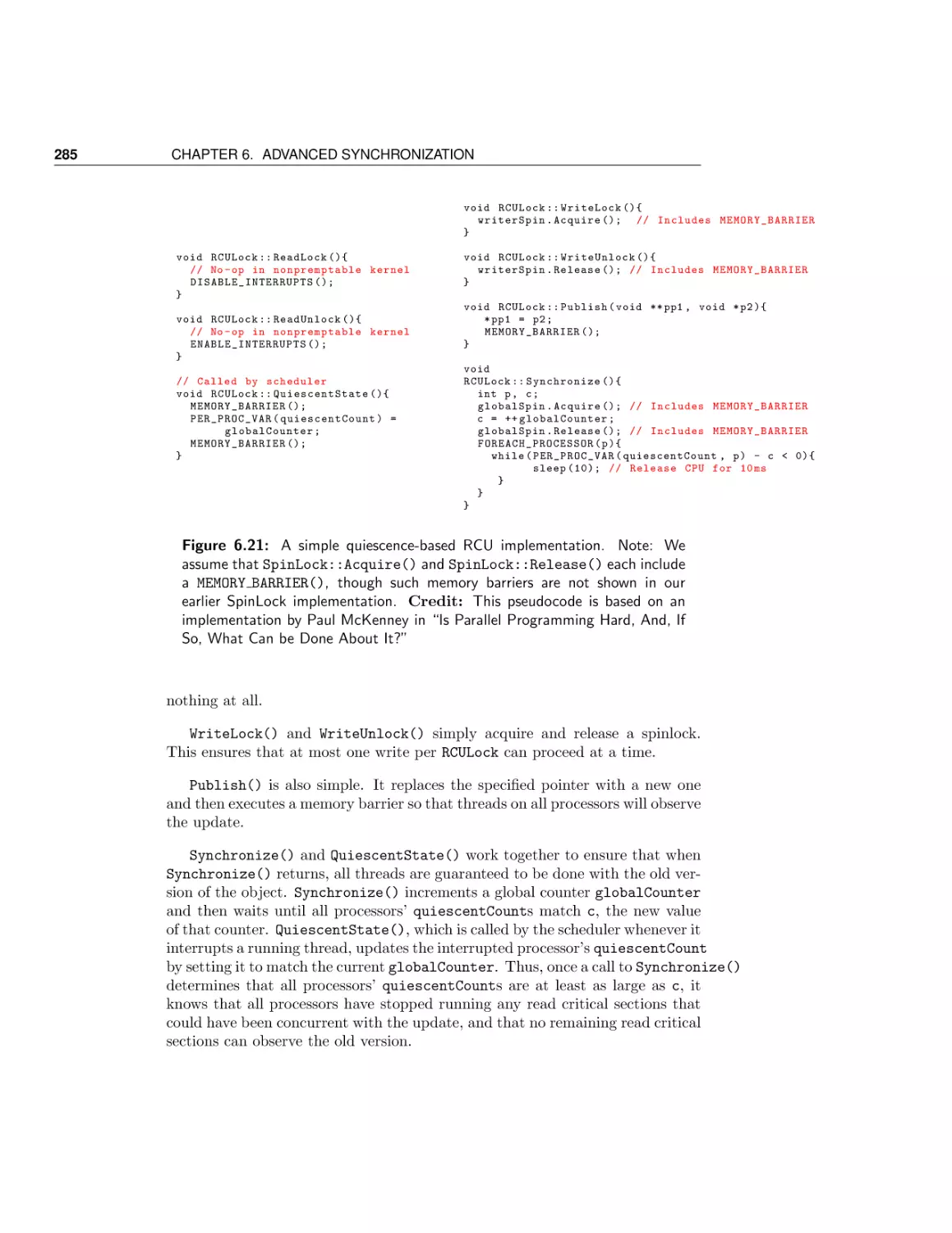
Chapter 6 discusses advanced topics in concurrency, including deadlock, synchronization across multiple objects, and advanced synchronization techniques
like read-copy-update (RCU). This is material is important for students to know,
but most semester-long operating systems courses will only be able to briefly
touch upon these issues.
Chapter 7 covers the concepts of resource allocation in the specific context of
Contents
viii
processor scheduling. After a quick tour through the tradeoffs between response
time and throughput for uniprocessor scheduling, the chapter covers a set of
more advanced topics in affinity and gang scheduling, power-aware and deadline
scheduling, as well as server scheduling, basic queueing theory and overload
management.
Chapter 8 explains hardware and software address translation mechanisms.
The first part of the chapter covers how to provide flexible memory management through multilevel segmentation and paging. Section 8.3 then considers
how hardware makes flexible memory management efficient through translation
lookaside buffers and virtually addressed caches, and how these are kept consistent as the operating system changes the addresses assigned to each process.
We conclude with a discussion of modern software-based protection mechanisms
such as those found in Android.
Chapter 9 covers caching and virtual memory. Caches are of course central
to many different types of computer systems. Most students will have seen the
concept of a cache in an earlier class machine structures, so our goal here is
to cover the theory and implementation of caches: when they work and when
they don’t, and how they are implemented in hardware and software. While
it might seem that we could skip virtual memory, many systems today provide
programmers the abstraction of memory-mapped files, and these rely on the
same mechanisms as in traditional virtual memory.
Chapter 10 discusses advanced topics in memory management. Address
translation hardware and software can be used for a number of different features in modern operating systems, such as zero copy I/O, copy on write, process checkpointing, and recoverable virtual memory. As this is more advanced
material, it can be skipped for time.
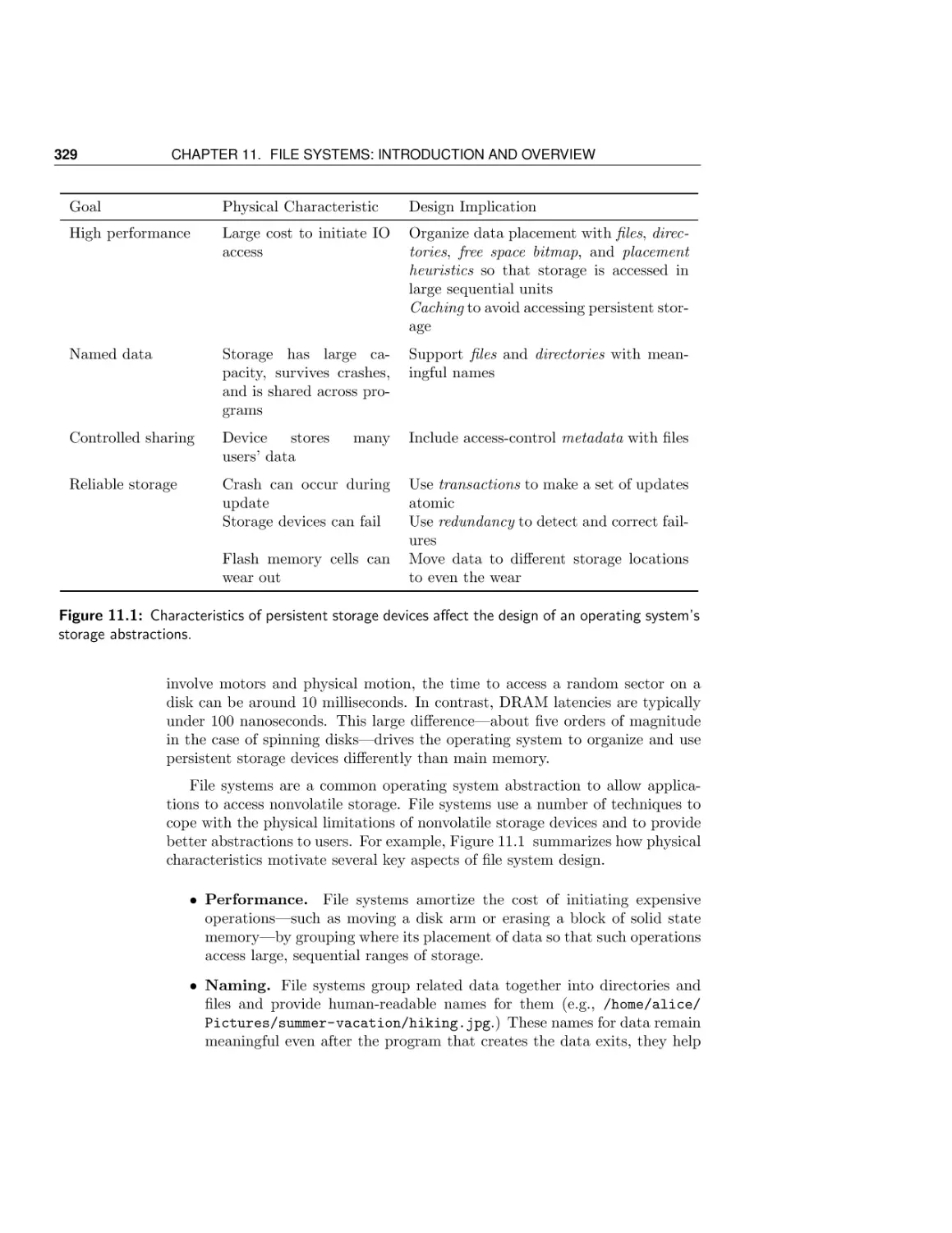
Chapter 11 sketches the characteristics of storage hardware, specifically block
storage devices such as magnetic disks and flash memory. The last two decades
have seen rapid change in storage technology affecting both application programmers and operating systems designers; this chapter provides a snapshot for
students, as a building block for the next two chapters. Classes in which students have taken a computer architecture course that covers these topics may
choose to skip this chapter.
Chapter 12 uses file systems as a case study of how complex data structures
can be organized on block storage devices to achieve flexibility and performance.
Chapter 13 explains the concept and implementation of reliable storage, using file systems as a concrete example. Starting with the ad hoc techniques in
UNIX fsck for implementing a reliable file system, the chapter explains checkpointing and write ahead logging as alternate implementation strategies for
building reliable storage, and it discusses how redundancy such as checksums
and replication are used to improve reliability and availability.
We are contemplating adding several chapters on networking and distributed
ix
CONTENTS
operating systems topics, but we are still considering what topics we can reasonably cover. We will be developing this material over the coming months.
Chapter 1
Introduction
“Everything I need to know I learned in kindergarten.” – Robert Fulgham
How do we construct reliable, portable, efficient and secure computer systems? An essential component is the computer’s operating system — the software that manages a computer’s resources.
First, the bad news: operating systems concepts are among the most complex
topics in computer science. A modern general-purpose operating system can run
to over 50 million lines of code, or in other words, more than a thousand times as
long as this textbook. New operating systems are being written all the time. If
you are reading this textbook on an e-book reader, tablet, or smartphone, there
is an operating system managing the device. Since we will not be able to cover
everything, our focus will be on the essential concepts for building computer
systems, ones that every computer scientist should know.
Now the good news: operating systems concepts are also among the most
accessible topics in computer science. Most of the topics in this book will seem
familiar to you — if you have ever tried to do two things at once, or picked
the wrong line at a grocery store, or tried to keep a roommate or sibling from
messing with your things, or succeeded at pulling off an April Fool’s joke. Each
of these has an analogue in operating systems, and it is this familiarity that
gives us hope that we can explain how operating systems do their work in a
single textbook. All we will assume of the reader is a basic understanding of
the operation of a computer and the ability to read pseudo-code.
We believe that understanding how operating systems work is essential for
any student interested in building modern computer systems. Of course, everyone who uses a computer or a smartphone or even a modern toaster uses an
1
2
2. Read
1. Get x.html
Server
Client
x.html
4. Data
3. Data
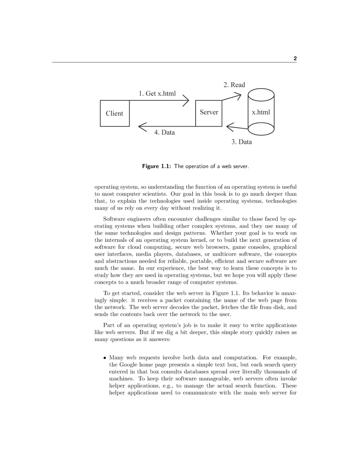
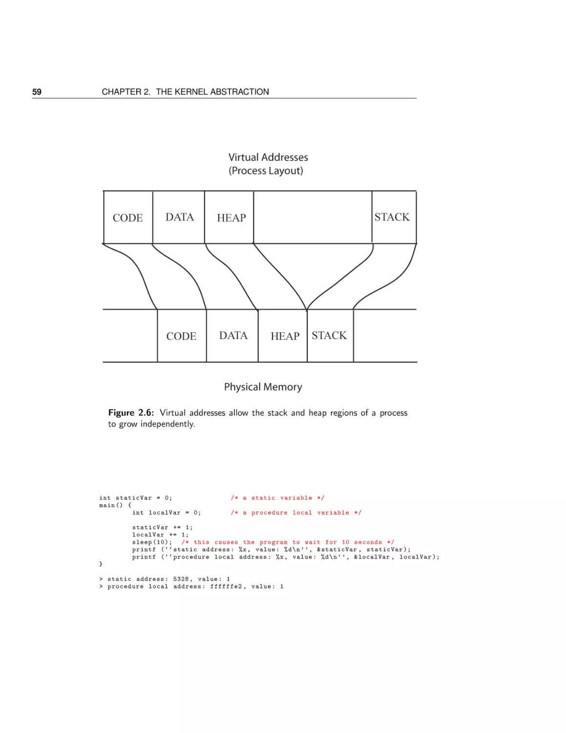
Figure 1.1: The operation of a web server.
operating system, so understanding the function of an operating system is useful
to most computer scientists. Our goal in this book is to go much deeper than
that, to explain the technologies used inside operating systems, technologies
many of us rely on every day without realizing it.
Software engineers often encounter challenges similar to those faced by operating systems when building other complex systems, and they use many of
the same technologies and design patterns. Whether your goal is to work on
the internals of an operating system kernel, or to build the next generation of
software for cloud computing, secure web browsers, game consoles, graphical
user interfaces, media players, databases, or multicore software, the concepts
and abstractions needed for reliable, portable, efficient and secure software are
much the same. In our experience, the best way to learn these concepts is to
study how they are used in operating systems, but we hope you will apply these
concepts to a much broader range of computer systems.
To get started, consider the web server in Figure 1.1. Its behavior is amazingly simple: it receives a packet containing the name of the web page from
the network. The web server decodes the packet, fetches the file from disk, and
sends the contents back over the network to the user.
Part of an operating system’s job is to make it easy to write applications
like web servers. But if we dig a bit deeper, this simple story quickly raises as
many questions as it answers:
• Many web requests involve both data and computation. For example,
the Google home page presents a simple text box, but each search query
entered in that box consults databases spread over literally thousands of
machines. To keep their software manageable, web servers often invoke
helper applications, e.g., to manage the actual search function. These
helper applications need to communicate with the main web server for
3
CHAPTER 1. INTRODUCTION
this to work. How does the operating system enable multiple applications
to commmunicate with each other?
• What if two users (or a million) try to request a web page from the server
at the same time? A simple approach might be to handle each request in
turn. If any individual request takes a long time, however, this approach
would mean that everyone else would need to wait for it to complete. A
faster, but more complex, solution is to multitask: to juggle the handling of
multiple requests at once. Multitasking is especially important on modern
multicore computers, as it provides a way to keep many processors busy.
How does the operating system enable applications to do multiple things
at once?
• For better performance, the web server might want to keep a copy, sometimes called a cache, of recently requested pages, so that the next user to
request the same page can be returned the results from the cache, rather
than starting the request from scratch. This requires the application to
synchronize access to the cache’s data structures by the thousands of web
requests being handled at the same time. How does the operating system
support application synchronization to shared data?
• To customize and animate the user experience, it is common for web
servers to send clients scripting code, along with the contents of the web
page. But this means that clicking on a link can cause someone else’s
code to run on your computer. How does the client operating system
protect itself from being compromised by a computer virus surreptitiously
embedded into the scripting code?
• Suppose the web site administrator uses an editor to update the web page.
The web server needs to be able to read the file that the editor wrote; how
does the operating system store the bytes on disk so that later on the web
server can find and read them?
• Taking this a step further, the administrator probably wants to be able to
make a consistent set of changes to the web site, so that embedded links
are not left dangling, even temporarily. How can the operating system
enable users to make a set of changes to a web site, so that requests either
see the old pages or the new pages, but not a mishmash of the two?
• What happens when the client browser and the web server run at different
speeds? If the server tries to send the web page to the client faster than
the client can draw the page, where are the contents of the file stored in
the meantime? Can the operating system decouple the client and server
so that each can run at its own speed, without slowing the other down?
• As demand on the web server grows, the administrator is likely to want
to move to more powerful hardware, with more memory, more processors,
faster network devices, and faster disks. To take advantage of this new
1.1. What is an operating system?
4
hardware, does the web server need to be re-written from scratch, or can it
be written in a hardware-independent fashion? What about the operating
system — does it need to be re-written for every new piece of hardware?
We could go on, but you get the idea. This book will help you understand
the answers to these questions, and more.
Goals of this chapter
The rest of this chapter discusses three topics in detail:
• OS Definition. What is an operating system and what does it do?
• OS Challenges. How should we evaluate operating systems, and what
are some of the tradeoffs their designers face?
• OS Past, Present and Future. What is the history of operating systems, and what new functionality are we likely to see in future operating
systems?
1.1
Definition: operating
system
What is an operating system?
An operating system is the layer of software that manages a computer’s resources
for its users and their applications. Operating systems run in a wide range of
computer systems. Sometimes they are invisible to the end user, controlling
embedded devices such as toasters, gaming systems, and the many computers
inside modern automobiles and airplanes. Operating systems are also an essential component of more general-purpose systems such as smartphones, desktop
computers, and servers.
Our discussion will focus on general-purpose operating systems, because the
technologies they need are a superset of the technologies needed for embedded systems. Increasingly though, technologies developed for general-purpose
computing are migrating into the embedded sphere. For example, early mobile phones had simple operating systems to manage the hardware and to run
a handful of primitive applications. Today, smartphones — phones capable of
running independent third party applications — are the fastest growing part
of the mobile phone business. These new devices require much more complete
operating systems, with sophisticated resource management, multi-tasking, security and failure isolation.
Likewise, automobiles are increasingly software controlled, raising a host of
operating system issues. Can anyone write software for your car? What if
the software fails while you are driving down the highway? How might the
operating system of your car be designed to prevent a computer virus from
5
CHAPTER 1. INTRODUCTION
A
P
P
A
P
P
A
P
P
Operating System
Hardware
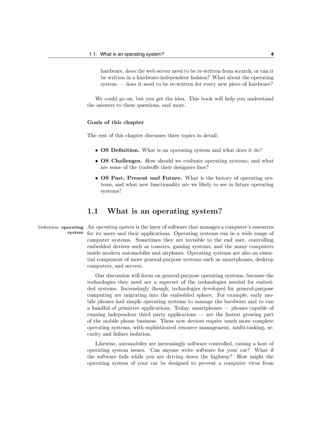
Figure 1.2: A general-purpose operating system
hijacking control of your car’s computers? Although this might seem far fetched,
researchers recently demonstrated that they could remotely turn off a car’s
braking system through a computer virus introduced into the car’s computers
through a hacked car radio. A goal of this book is to explain how to build more
reliable and secure computer systems in a variety of contexts.
For general-purpose systems, users interact with applications, applications
execute in an environment provided by the operating system, and the operating
system mediates access to the underlying hardware (Figure 1.2, and expanded
in Figure 1.3). What do we need from an operating system to be able to run a
group of programs? Operating systems have three roles:
• Operating systems play referee — they manage shared resources between
different applications running on the same physical machine. For example,
an operating system can stop one program and start another. Operating
systems isolate different applications from each other, so that if there is
a bug in one application, it does not corrupt other applications running
on the same machine. The operating system must protect itself and other
applications from malicious computer viruses. And since the applications
1.1. What is an operating system?
6
An Expanded View of an Operating System
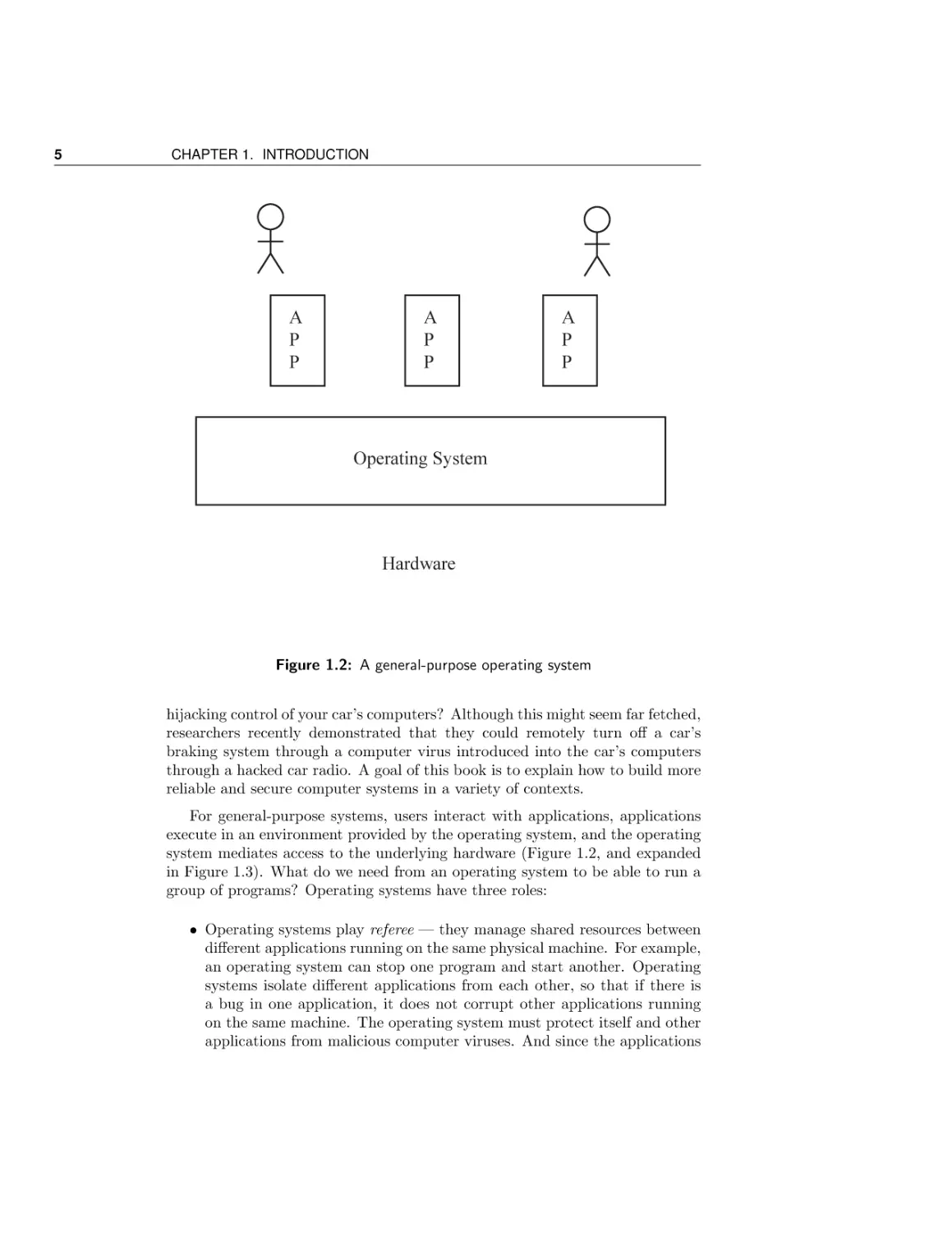
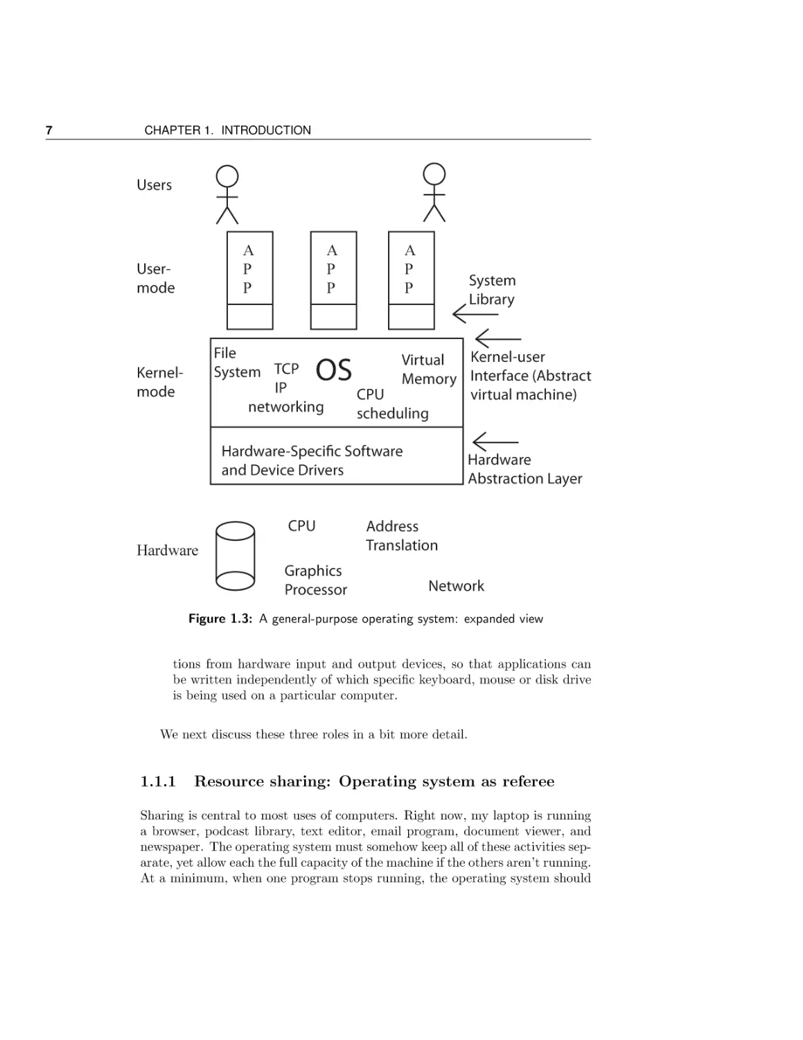
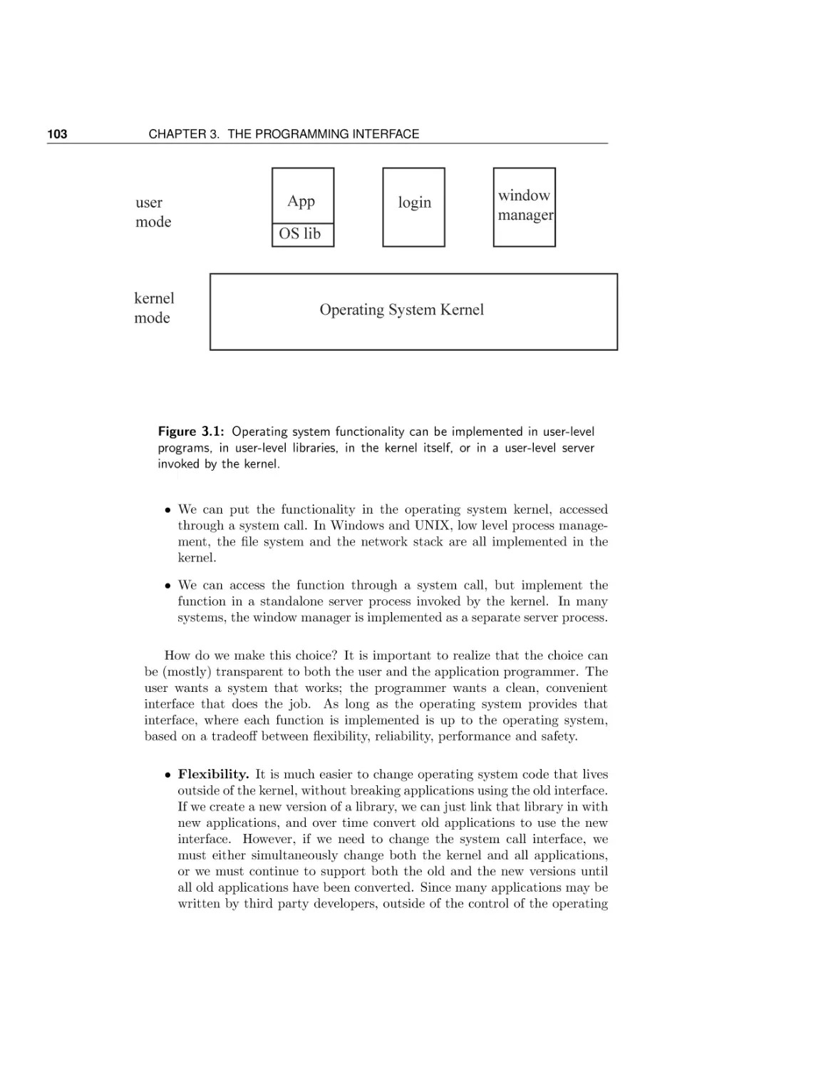
Figure 1.3 shows the structure of a general-purpose operating system, as an expansion on the simple view presented in Figure 1.2. At the lowest level, the hardware provides processor, memory, and a set of devices for providing the user interface, storing
data and communicating with the outside world. The hardware also provides primitives that the operating system can use to provide fault isolation and synchronization.
The operating system runs as the lowest layer of software on the computer, with a
device-specific layer interfaces to the myriad hardware devices, and a set of deviceindependent services provided to applications. Since the operating system needs to be
able to isolate malicious and buggy applications from affecting other applications or the
operating system itself, much of the operating system runs in a separate execution environment protected from application code. A portion of the operating system can also
run as a library linked into each application. In turn, applications run in an execution
context provided by the operating system. The application context is much more than
a simple abstraction on top of hardware devices: applications execute in a virtual environment that is both more constrained (to prevent harm), more powerful (to mask hardware limitations), and more useful (via common services), than the underlying hardware.
are sharing physical resources, the operating system needs to decide which
applications get which resources.
• Operating systems play illusionist — they provide an abstraction physical hardware to simplify application design. To write a “hello world”
program, you do not need (or want!) to think about how much physical
memory the system has, or how many other programs might be sharing
the computer’s resources. Instead, operating systems provide the illusion
of a nearly infinite memory, as an abstraction on top of a limited amount
of physical memory. Likewise, operating systems provide the illusion that
each program has the computer’s processors entirely to itself. Obviously,
the reality is quite different! These illusions enable applications to be
written independently of the amount of physical memory on the system
or the physical number of processors. Because applications are written to
a higher level of abstraction, the operating system is free to change the
amount of resources assigned to each application as applications start and
stop.
• Operating systems provide glue — a set of common services between applications. An important benefit of common services is to facilitate sharing
between applications, so that, for example, cut and paste works uniformly
across the system and a file written by one application can be read by
another. Many operating systems provide a common set of user interface
routines to help applications provide a common “look and feel.” Perhaps
most importantly, operating systems provide a layer separating applica-
7
CHAPTER 1. INTRODUCTION
Users
A
P
P
Usermode
A
P
P
File
System TCP
IP
networking
OS
Kernelmode
A
P
P
System
Library
Kernel-user
Virtual
Memory Interface (Abstract
CPU
virtual machine)
scheduling
Hardware-Specific Software
and Device Drivers
CPU
Hardware
Graphics
Processor
Hardware
Abstraction Layer
Address
Translation
Network
Figure 1.3: A general-purpose operating system: expanded view
tions from hardware input and output devices, so that applications can
be written independently of which specific keyboard, mouse or disk drive
is being used on a particular computer.
We next discuss these three roles in a bit more detail.
1.1.1
Resource sharing: Operating system as referee
Sharing is central to most uses of computers. Right now, my laptop is running
a browser, podcast library, text editor, email program, document viewer, and
newspaper. The operating system must somehow keep all of these activities separate, yet allow each the full capacity of the machine if the others aren’t running.
At a minimum, when one program stops running, the operating system should
1.1. What is an operating system?
8
let me run another. Better, the operating system should allow multiple applications to run at the same time, as when I read email while I am downloading
a security patch to the system software.
Even individual applications can be designed to do multiple things at once.
For instance, a web server will be more responsive to its users if it can handle
multiple requests at the same time rather than waiting for each to complete
before the next one starts running. The same holds for the browser — it is
more responsive if it can start drawing a page while the rest of the page is
still being transferred. On multiprocessors, the computation inside a parallel
application can be split into separate units that can be run independently for
faster execution. The operating system itself is an example of software written
to be able to do multiple things at once. As we will describe later, the operating
system is a customer of its own abstractions.
Sharing raises several challenges for an operating system:
• Resource Allocation. The operating system must keep all of the simultaneous activities separate, allocating resources to each as appropriate. A
computer usually has only a few processors and a finite amount of memory,
network bandwidth, and disk space. When there are multiple tasks to do
at the same time, how should the operating system choose how many resources to give to each? Seemingly trivial differences in how resources are
allocated can have a large impact on user-perceived performance. As we
will see later, if the operating system gives too little memory to a program,
it will not only slow down that particular program, it can dramatically
hurt the performance of the entire machine.
As another example, what should happen if an application executes an
infinite loop:
while ( true ){
;
}
If programs ran directly on the raw hardware, this code fragment would
lock up the computer, making it completely non-responsive to user input.
With resource multiplexing provided by the operating system, the specific
application might lock up, but other programs can proceed unimpeded.
Additionally, the user can ask the operating system to force the looping
program to exit.
Definition: fault isolation
• Isolation. An error in one application should not disrupt other applications, or even the operating system itself. This is called fault isolation.
Anyone who has taken an introductory computer science class knows the
value of an operating system that can protect itself and other applications
from programmer bugs. Debugging would be vastly harder if an error
9
CHAPTER 1. INTRODUCTION
in one program could corrupt data structures in other applications. Likewise, downloading and installing a screen saver or other application should
not crash other unrelated programs, nor should it be a way for a malicious attacker to surreptitiously install a computer virus on the system.
Nor should one user be able to access or change another’s data without
permission.
Fault isolation requires restricting the behavior of applications to less than
the full power of the underlying hardware. Given access to the full capability of the hardware, any application downloaded off the web, or any script
embedded in a web page, would have complete control of the machine.
Thus, it would be able to install spyware into the operating system to
log every keystroke you type, or record the password to every website you
visit. Without fault isolation provided by the operating system, any bug
in any program might cause the disk to become irretrievably corrupted.
Erroneous or malignant applications would cause all sorts of havoc.
• Communication. The flip side of isolation is the need for communication
between different applications and between different users. For example, a
web site may be implemented by a cooperating set of applications: one to
select advertisements, another to cache recent results, yet another to fetch
and merge data from disk, and several more to cooperatively scan the web
for new content to index. For this to work, the various programs need
to be able to communicate with one another. If the operating systems
is designed to prevent bugs and malicious users and applications from
affecting other users and their applications, how does the operating system
support communication to share results? In setting up boundaries, an
operating system must also allow for those boundaries to be crossed in
carefully controlled ways as the need arises.
In its role as a referee, an operating system is somewhat akin to that of a
government, or perhaps a particularly patient kindergarten teacher, balancing
needs, separating conflicts, and facilitating sharing. One user should not be
able to hog all of the system’s resources or to access or corrupt another user’s
files without permission; a buggy application should not be able to crash the
operating system or other unrelated applications; and yet applications also need
to be able to work together. Enforcing and balancing these concerns is the role
of the operating system.
Exercises
Take a moment to speculate. We will provide answers to these questions
throughout the rest of the book, but given what you know now, how would you
answer them? Before there were operating systems, someone needed to develop
solutions, without being able to look them up! How would you have designed
the first operating system?
1.1. What is an operating system?
10
1. Suppose a computer system and all of its applications are completely bug
free. Suppose further that everyone in the world is completely honest and
trustworthy. In other words, we do not need to consider fault isolation.
a. How should the operating system allocate time on the processor?
Should it give all of the processor to each application until it no
longer needs it? If there are multiple tasks ready to go at the same
time, should it schedule the task with the least amount of work to
do or the one with the most? Justify your answer.
b. How should the operating system allocate physical memory between
applications? What should happen if the set of applications do not
all fit in memory at the same time?
c. How should the operating system allocate its disk space? Should the
first user to ask be able to grab all of the free space? What would
the likely outcome be for that policy?
2. Now suppose the computer system needs to support fault isolation. What
hardware and/or operating support do you think would be needed to accomplish this goal?
a. For protecting an application’s data structures in memory from being
corrupted by other applications?
b. For protecting one user’s disk files from being accessed or corrupted
by another user?
c. For protecting the network from a virus trying to use your computer
to send spam?
3. How should an operating system support communication between applications?
a. Through the file system?
b. Through messages passed between applications?
c. Through regions of memory shared between the applications?
d. All of the above? None of the above?
1.1.2
Mask hardware limitations: Operating system as illusionist
A second important role of operating systems is to mask the restrictions inherent
in computer hardware. Hardware is necessarily limited by physical constraints
— a computer has only a limited number of processors and a limited amount
11
CHAPTER 1. INTRODUCTION
A
P
P
A
P
P
Guest
Operating
System
A
P
P
Guest
Operating
System
Operating System
Hardware
Figure 1.4: An operating system virtual machine
of physical memory, network bandwidth, and disk. Further, since the operating
system must decide how to split the fixed set of resources among the various
applications running at each moment, a particular application will have different amounts of resources from time to time, even when running on the same
hardware. While a few applications might be designed to take advantage of a
computer’s specific hardware configuration and their specific resource assignment, most programmers want to use a higher level of abstraction.
We have just discussed one example of this: a uniprocessor can run only one
program at a time, yet most operating systems allow multiple applications to
appear to the user to be running at the same time. The operating system does so
through a concept called virtualization. Virtualization provides an application Definition: virtualization
with the illusion of resources that are not physically present. For example, the
operating system can present to each application the abstraction that it has an
entire processor dedicated to it, even though at a physical level there may be only
a single processor shared among all the applications running on the computer.
With the right hardware and operating system support, most physical resources
can be virtualized: examples include the processor, memory, screen space, disk,
and the network. Even the type of processor can be virtualized, to allow the
same, unmodified application to be run on a smartphone, tablet, and laptop
computer.
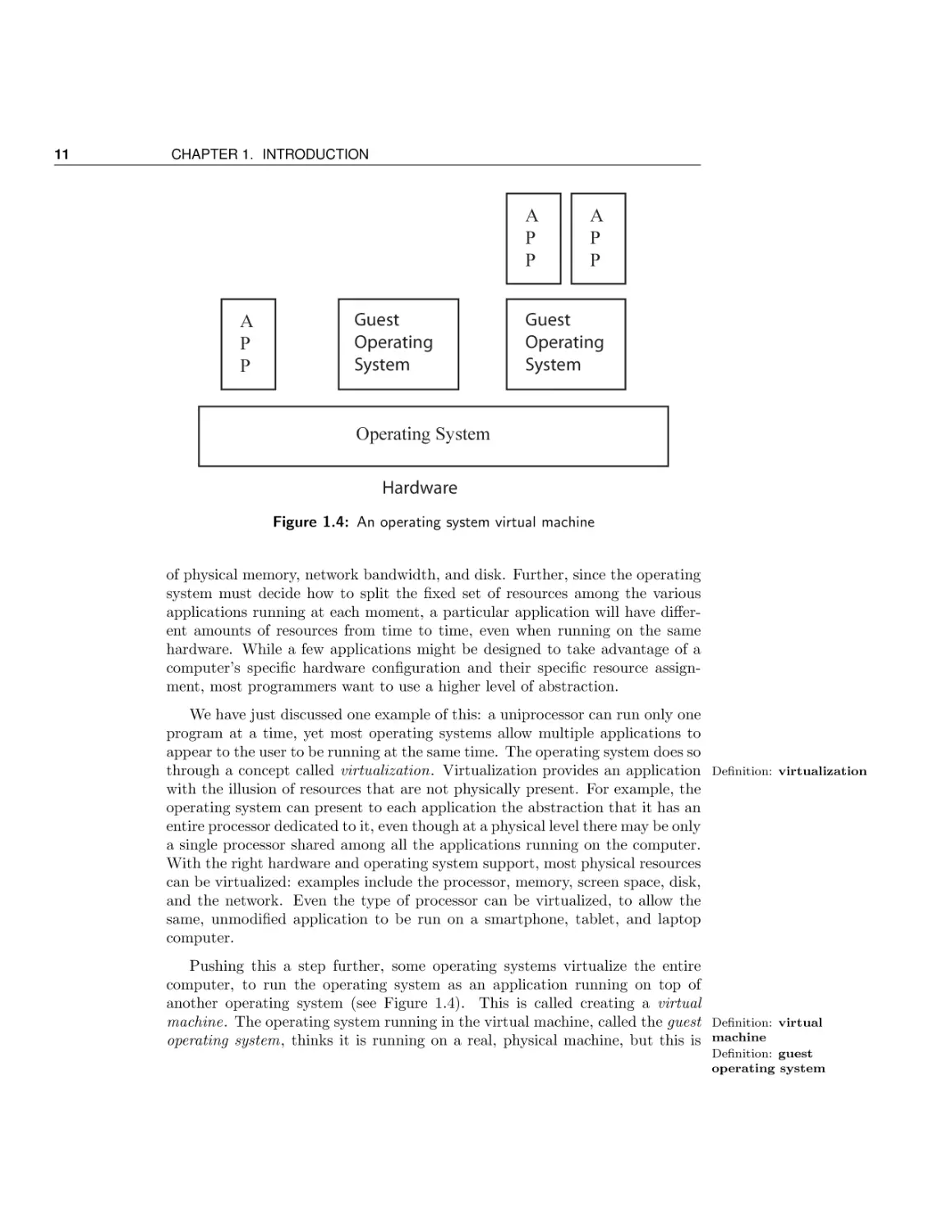
Pushing this a step further, some operating systems virtualize the entire
computer, to run the operating system as an application running on top of
another operating system (see Figure 1.4). This is called creating a virtual
machine. The operating system running in the virtual machine, called the guest Definition: virtual
operating system, thinks it is running on a real, physical machine, but this is machine
Definition: guest
operating system
1.1. What is an operating system?
12
an illusion presented by the true operating system running underneath. One
reason for the operating system to provide a virtual machine is for application
portability. If a program only runs on an old version of an operating system,
then we can still run the program on a new system running a virtual machine.
The virtual machine hosts the application on the old operating system, running
on top of the new operating system. Another reason for virtual machines is as
an aid in debugging. If an operating system can be run as an application, then
the operating system developers can set breakpoints, stop, and single step their
code just as they would an application.
In addition to virtualization, operating systems mask many other limitations inherent in physical hardware, by providing applications with the illusion
of hardware capabilities that are not physically present. For example, on a computer with multiple processors sharing memory, each processor can update only
a single memory location at a time. The memory system in hardware ensures
Definition: atomic that any updates to the same memory word are atomic, that is, the value stored
in memory is the last value stored by one of the processors, not a mixture of the
updates of the different processors. Atomicity at the level of a memory word
is preserved in hardware even if more than one processor attempts to write to
memory at exactly the same time. While this might seem sufficient, applications (and the operating system itself) need to be able to update larger data
structures, ones spread over many memory locations. What happens when two
processors attempt to update the same data structure at roughly the same time?
As we’ll discuss later, the results can be quite unexpected and quite different
from what would have happened had each of the processors updated the data
structure in turn. Ideally, the programmer would like to have the abstraction
of an atomic update to the entire data structure, not just to a single memory
word. As we will discuss, the illusion of atomic updates to data structures is
provided by the operating system using some specialized mechanisms provided
in hardware.
Persistent block storage devices, such as magnetic disk or flash RAM, provide
another example. At a physical level, these systems support block writes to
storage, where the size of the block depends on physical device characteristics.
If the computer crashes in the middle of a block write, it could leave the disk
in an unknown state, with neither the old nor the new value stored at that
location. Of course, applications need to be able to store data on disk that is
variable in size, possibly spanning multiple disk blocks. And users want their
data to be preserved even — or especially — if there is a machine failure while
the disk is being updated.
We will discuss techniques that the operating system uses to accomplish
these and other illusions. In each of these cases, the operating system provides
a more convenient and flexible programming abstraction than what is provided
by the underlying hardware.
13
CHAPTER 1. INTRODUCTION
Exercises
Take a moment to speculate; to build the systems we use today, someone
needed to answer these questions. Consider how you might answer them, before
seeing how others solved these puzzles.
4. How would you design combined hardware and software support to provide
the illusion of a nearly infinite virtual memory on a limited amount of
physical memory?
5. How would you design a system to run an entire operating system as an
application running on top of another operating system?
6. How would you design a system to update complex data structures on
disk in a consistent fashion despite machine crashes?
1.1.3
Common services: Operating system as glue
Operating system also play a third role: providing a set of common, standard
services to applications to simplify and regularize their design. We saw an
example of this with the web server outlined at the beginning of this chapter.
The operating system hides the specifics of how the network and disk devices
work, providing a simpler abstraction to applications based on receiving and
sending reliable streams of bytes, and reading and writing named files. This
allows the web server can focus on its core task of decoding incoming requests
and filling them, rather than on the formatting of data into individual network
packets and disk blocks.
An important reason for the operating system to provide common services,
rather than leaving it up to each application, is to facilitate sharing between
applications. The web server needs to be able to read the file that the text editor
wrote. If applications are to share files, they need to be stored in a standard
format, with a standard system for managing file directories. Likewise, most
operating systems provide a standard way for applications to pass messages,
and to share memory, to facilitate sharing.
The choice of which services an operating system should provide is often a
matter of judgment. For example, computers can come configured with a blizzard of different devices: different graphics co-processors and pixel formats, different network interfaces (WiFi, Ethernet, and Bluetooth), different disk drives
(SCSI, IDE), different device interfaces (USB, Firewire), and different sensors
(GPS, accelerometers), not to mention different versions of each of those standards. Most applications will be able to ignore these differences, using only
a generic interface provided by the operating system. For other applications,
1.1. What is an operating system?
14
such as a database, the specific disk drive may matter quite a bit. For those
applications that can operate at a higher level of abstraction, the operating
system serves as an interoperability layer, so that both applications, and the
devices themselves, can be independently evolved without requiring simultaneous changes to the other side.
Another standard service in most modern operating systems is the graphical
user interface library. Both Microsoft’s and Apple’s operating systems provide
a set of standard user interface widgets. This facilitates a common “look and
feel” to users, so that frequent operations such as pull down menus and “cut”
and “paste” are handled consistently across applications.
Most of the code of an operating system is to implement these common services. However, much of the complexity of operating systems is due to resource
sharing and masking hardware limits. Because the common service code is built
on the abstractions provided by the other two operating system roles, this book
will focus primarily on those two topics.
1.1.4
Operating system design patterns
The challenges that operating systems address are not unique — they apply
to many different computer domains. Many complex software systems have
multiple users, run programs written by third party developers, and/or need
to coordinate many simultaneous activities. These pose questions of resource
allocation, fault isolation, communication, abstractions of physical hardware,
and how to provide a useful set of common services for software developers.
Not only are the challenges the same, but often the solutions are as well: these
systems use many of the design patterns and techniques described in this book.
For now, we focus on the challenges these systems have in common with
operating systems:
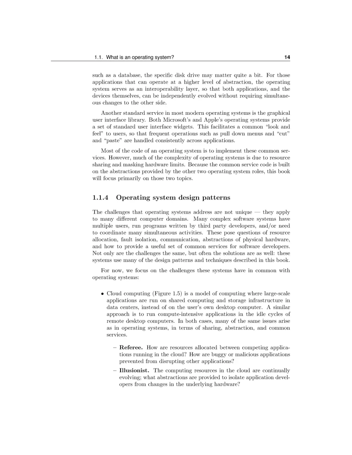
• Cloud computing (Figure 1.5) is a model of computing where large-scale
applications are run on shared computing and storage infrastructure in
data centers, instead of on the user’s own desktop computer. A similar
approach is to run compute-intensive applications in the idle cycles of
remote desktop computers. In both cases, many of the same issues arise
as in operating systems, in terms of sharing, abstraction, and common
services.
– Referee. How are resources allocated between competing applications running in the cloud? How are buggy or malicious applications
prevented from disrupting other applications?
– Illusionist. The computing resources in the cloud are continually
evolving; what abstractions are provided to isolate application developers from changes in the underlying hardware?
15
CHAPTER 1. INTRODUCTION
A
P
P
A
P
P
A
P
P
Cloud Software
Server
Server
Server
Server
Figure 1.5: Cloud computing
– Glue. Cloud services often distribute their work across different machines. What abstractions should the cloud software provide to help
services coordinate and share data between their various activities?
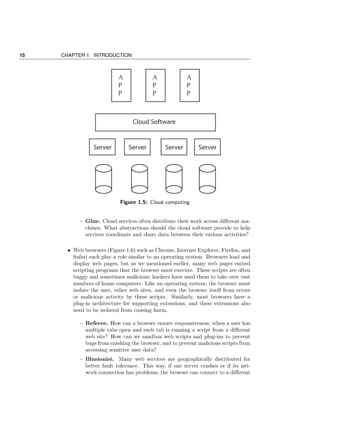
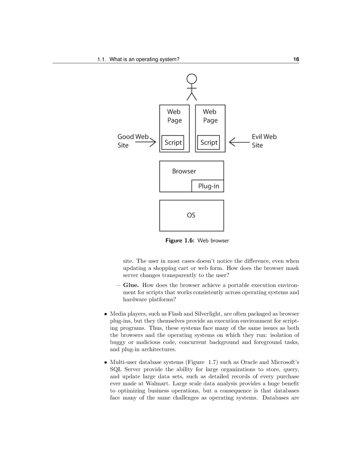
• Web browsers (Figure 1.6) such as Chrome, Internet Explorer, Firefox, and
Safari each play a role similar to an operating system. Browsers load and
display web pages, but as we mentioned earlier, many web pages embed
scripting programs that the browser must execute. These scripts are often
buggy and sometimes malicious; hackers have used them to take over vast
numbers of home computers. Like an operating system, the browser must
isolate the user, other web sites, and even the browser itself from errors
or malicious activity by these scripts. Similarly, most browsers have a
plug-in architecture for supporting extensions, and these extensions also
need to be isolated from causing harm.
– Referee. How can a browser ensure responsiveness, when a user has
multiple tabs open and each tab is running a script from a different
web site? How can we sandbox web scripts and plug-ins to prevent
bugs from crashing the browser, and to prevent malicious scripts from
accessing sensitive user data?
– Illusionist. Many web services are geographically distributed for
better fault tolerance. This way, if one server crashes or if its network connection has problems, the browser can connect to a different
16
1.1. What is an operating system?
Good Web
Site
Web
Page
Web
Page
Script
Script
Evil Web
Site
Browser
Plug-in
OS
Figure 1.6: Web browser
site. The user in most cases doesn’t notice the difference, even when
updating a shopping cart or web form. How does the browser mask
server changes transparently to the user?
– Glue. How does the browser achieve a portable execution environment for scripts that works consistently across operating systems and
hardware platforms?
• Media players, such as Flash and Silverlight, are often packaged as browser
plug-ins, but they themselves provide an execution environment for scripting programs. Thus, these systems face many of the same issues as both
the browsers and the operating systems on which they run: isolation of
buggy or malicious code, concurrent background and foreground tasks,
and plug-in architectures.
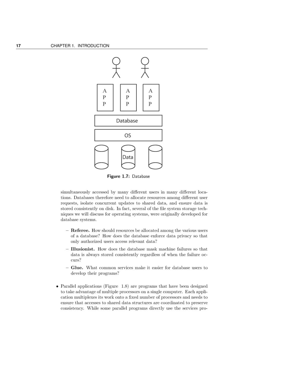
• Multi-user database systems (Figure 1.7) such as Oracle and Microsoft’s
SQL Server provide the ability for large organizations to store, query,
and update large data sets, such as detailed records of every purchase
ever made at Walmart. Large scale data analysis provides a huge benefit
to optimizing business operations, but a consequence is that databases
face many of the same challenges as operating systems. Databases are
17
CHAPTER 1. INTRODUCTION
A
P
P
A
P
P
A
P
P
Database
OS
Data
Figure 1.7: Database
simultaneously accessed by many different users in many different locations. Databases therefore need to allocate resources among different user
requests, isolate concurrent updates to shared data, and ensure data is
stored consistently on disk. In fact, several of the file system storage techniques we will discuss for operating systems, were originally developed for
database systems.
– Referee. How should resources be allocated among the various users
of a database? How does the database enforce data privacy so that
only authorized users access relevant data?
– Illusionist. How does the database mask machine failures so that
data is always stored consistently regardless of when the failure occurs?
– Glue. What common services make it easier for database users to
develop their programs?
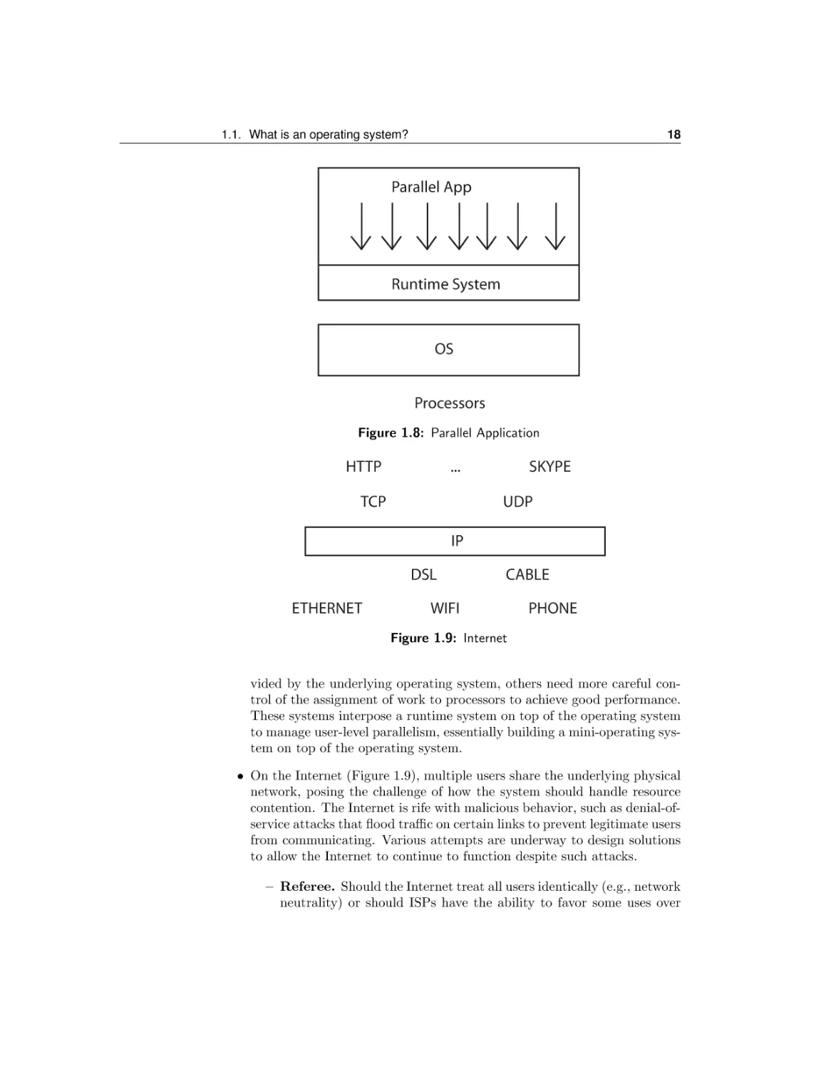
• Parallel applications (Figure 1.8) are programs that have been designed
to take advantage of multiple processors on a single computer. Each application multiplexes its work onto a fixed number of processors and needs to
ensure that accesses to shared data structures are coordinated to preserve
consistency. While some parallel programs directly use the services pro-
18
1.1. What is an operating system?
Parallel App
Runtime System
OS
Processors
Figure 1.8: Parallel Application
HTTP
...
TCP
SKYPE
UDP
IP
DSL
ETHERNET
CABLE
WIFI
PHONE
Figure 1.9: Internet
vided by the underlying operating system, others need more careful control of the assignment of work to processors to achieve good performance.
These systems interpose a runtime system on top of the operating system
to manage user-level parallelism, essentially building a mini-operating system on top of the operating system.
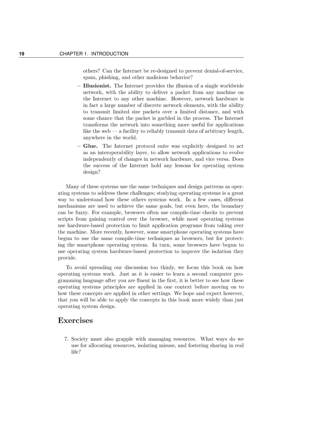
• On the Internet (Figure 1.9), multiple users share the underlying physical
network, posing the challenge of how the system should handle resource
contention. The Internet is rife with malicious behavior, such as denial-ofservice attacks that flood traffic on certain links to prevent legitimate users
from communicating. Various attempts are underway to design solutions
to allow the Internet to continue to function despite such attacks.
– Referee. Should the Internet treat all users identically (e.g., network
neutrality) or should ISPs have the ability to favor some uses over
19
CHAPTER 1. INTRODUCTION
others? Can the Internet be re-designed to prevent denial-of-service,
spam, phishing, and other malicious behavior?
– Illusionist. The Internet provides the illusion of a single worldwide
network, with the ability to deliver a packet from any machine on
the Internet to any other machine. However, network hardware is
in fact a large number of discrete network elements, with the ability
to transmit limited size packets over a limited distance, and with
some chance that the packet is garbled in the process. The Internet
transforms the network into something more useful for applications
like the web — a facility to reliably transmit data of arbitrary length,
anywhere in the world.
– Glue. The Internet protocol suite was explicitly designed to act
as an interoperability layer, to allow network applications to evolve
independently of changes in network hardware, and vice versa. Does
the success of the Internet hold any lessons for operating system
design?
Many of these systems use the same techniques and design patterns as operating systems to address these challenges; studying operating systems is a great
way to understand how these others systems work. In a few cases, different
mechanisms are used to achieve the same goals, but even here, the boundary
can be fuzzy. For example, browsers often use compile-time checks to prevent
scripts from gaining control over the browser, while most operating systems
use hardware-based protection to limit application programs from taking over
the machine. More recently, however, some smartphone operating systems have
begun to use the same compile-time techniques as browsers, but for protecting the smartphone operating system. In turn, some browsers have begun to
use operating system hardware-based protection to improve the isolation they
provide.
To avoid spreading our discussion too thinly, we focus this book on how
operating systems work. Just as it is easier to learn a second computer programming language after you are fluent in the first, it is better to see how these
operating systems principles are applied in one context before moving on to
how these concepts are applied in other settings. We hope and expect however,
that you will be able to apply the concepts in this book more widely than just
operating system design.
Exercises
7. Society must also grapple with managing resources. What ways do we
use for allocating resources, isolating misuse, and fostering sharing in real
life?
1.2. Evaluation Criteria
1.2
20
Evaluation Criteria
Having defined what an operating system does, how should we choose among
alternative approaches to the design challenges posed by operating systems?
We next discuss several desirable criteria for operating systems. In many cases,
tradeoffs between these criteria are inevitable — improving a system along one
dimension will hurt it along another. We conclude with a discussion of some
concrete examples of tradeoffs between these considerations.
1.2.1
Definition: Reliability
Reliability
Perhaps the most important characteristic of an operating system is its reliability. Reliability is that a system does exactly what it is designed to do. As the
lowest level of software running on the system, errors in operating system code
can have devastating and hidden effects. If the operating system breaks, the
user will often be unable to get any work done, and in some cases, may even lose
previous work, e.g., if the failure corrupts files on disk. By contrast, application
failures can be much more benign, precisely because operating systems provides
fault isolation and a rapid and clean restart after an error.
Making the operating system reliable is challenging. Operating systems often
operate in a hostile environment, where computer viruses and other malicious
code may often be trying to take control of the system for their own purposes by
exploiting design or implementation errors in the operating system’s defenses.
Unfortunately, the most common ways for improving software reliability,
such as running test cases for common code paths, are less effective when applied
to operating systems. Since malicious attacks can target a specific vulnerability
precisely to cause execution to follow a rare code path, literally everything has to
work correctly for the operating system to be reliable. Even without malicious
attacks that trigger bugs on purpose, extremely rare corner cases can occur
regularly in the operating system context. If an operating system has a million
users, a once in a billion event will eventually occur to someone.
Definition: availability
A related concept is availability, the percentage of time that the system is usable. A buggy operating system that crashes frequently, losing the user’s work,
is both unreliable and unavailable. A buggy operating system that crashes frequently, but never loses the user’s work and cannot be subverted by a malicious
attack, would be reliable but unavailable. An operating system that has been
subverted, but continues to appear to run normally while logging the user’s
keystrokes, is unreliable but available.
Thus, both reliability and availability are desirable. Availability is affected
by two factors: the frequency of failures, called the mean time to failure (MTTF)Definition: mean time to , and the time it takes to restore a system to a working state after a failure (for
failure (MTTF) example, to reboot), the mean time to repair (MTTR). Availability can be imDefinition: mean time to
repair (MTTR)
21
CHAPTER 1. INTRODUCTION
proved by increasing the MTTF or reducing the MTTR, and we will present
operating systems techniques that do each.
Throughout this book, we will present various approaches to improving operating system reliability and availability. In many cases, the abstractions may
seem at first glance overly rigid and formulaic. It is important to realize this
is done on purpose! Only precise abstractions provide a basis for constructing
reliable and available systems.
Exercises
8. Suppose you were tasked with designing and implementing an ultra-reliable
and ultra-available operating system. What techniques would you use?
What tests, if any, might be sufficient to convince you of the system’s
reliability, short of handing your operating system to millions of users to
serve as beta testers?
9. MTTR, and therefore availability, can be improved by reducing the time
to reboot a system after a failure. What techniques might you use to
speed up booting? Would your techniques always work after a failure?
1.2.2
Security
Two concepts closely related to reliability are security and privacy. Securityis the property that the computer’s operation cannot be compromised by a Definition: Security
malicious attacker. Privacy is a part of security — that data stored on the Definition: Privacy
computer is only accessible to authorized users.
Alas, no useful computer is perfectly secure! Any complex piece of software
has bugs, and even otherwise innocuous bugs can be exploited by an attacker to
gain control of the system. Or the hardware of the computer might be tampered
with, to provide access to the attacker. Or the computer’s administrator might
turn out to be untrustworthy, using their privileges to steal user data. Or the
software developer of the operating system might be untrustworthy, inserting a
backdoor for the attacker to gain access to the system.
Nevertheless, an operating system can, and should, be designed to minimize
its vulnerability to attack. For example, strong fault isolation can prevent third
party applications from taking over the system. Downloading and installing
a screen saver or other application should not provide a way for a malicious
attacker to surreptitiously install a computer virus on the system. A computer Definition: computer virus
virus is a computer program that modifies an operating system or application
to provide the attacker, rather than the user, control over the system’s resources
1.2. Evaluation Criteria
22
or data. An example computer virus is a keylogger: a program that modifies
the operating system to record every keystroke entered by the user and send
those keystrokes back to the attacker’s machine. In this way, the attacker could
gain access to the user’s passwords, bank account numbers, and other private
information. Likewise, a malicious screen saver might surreptiously scan the
disk for files containing personal information or turn the system into an email
spam server.
Even with strong fault isolation, a system can be insecure if its applications
are not designed for security. For example, the Internet email standard provides
no strong assurance of the sender’s identity; it is possible to form an email message with anyone’s email address in the “from” field, not necessarily the actual
sender. Thus, an email message can appear to be from someone (perhaps someone you trust), when in reality it is from someone else (and contains a malicious
virus that takes over the computer when the attachment is opened). By now,
you are hopefully suspicious of clicking on any attachment in an email. If we
step back, though, the issue could instead be cast as a limitation of the interaction between the email system and the operating system — if the operating
system provided a cheap and easy way to process an attachment in an isolated
execution environment with limited capabilities, then even if the attachment
contained a virus, it would be guaranteed not to cause a problem.
Complicating matters is that the operating system must not only prevent
unwanted access to shared data, it must also allow access in many cases. We
want users and programs to interact with each other, to be able to cut and paste
text between different applications, and to read or write data to disk or over
the network. If each program was completely standalone, and never needed to
interact with any other program, then fault isolation by itself would be enough.
However, we not only want to be able to isolate programs from one another, we
also want to be able to easily share data between programs and between users.
Definition: enforcement
Definition: security policy
Thus, an operating system needs both an enforcement mechanism and a
security policy. Enforcement is how the operating system ensures that only
permitted actions are allowed. The security policy defines what is permitted
— who is allowed to access what data and who can perform what operations.
Malicious attackers can target vulnerabilities in either enforcement mechanisms
or security policy.
1.2.3
Definition: portable
Portability
All operating systems provide applications an abstraction of the underlying
computer hardware; a portable abstraction is one that does not change as the
hardware changes. A program written for Microsoft’s Windows 7 should run
correctly regardless of whether a specific graphics card is being used, whether
persistent storage is provided via flash memory or rotating magnetic disk, or
whether the network is Bluetooth, WiFi, or gigabit Ethernet.
23
CHAPTER 1. INTRODUCTION
Portability also applies to the operating system itself. Operating systems are
among the most complex software systems ever invented, so it is impractical to
re-write them from scratch every time some new hardware is produced or every
time a new application is developed. Instead, new operating systems are often
derived, at least in part, from old ones. As one example, iOS, the operating
system for the iPhone and iPad, is derived from the OS X code base.
As a result, most successful operating systems have a lifetime measured in
decades: the initial implementation of Microsoft Windows 8 began with the
development of Windows NT starting in 1990, when the typical computer was
more than 10000 times less powerful and had 10000 times less memory and
disk storage, than is the case today. Operating systems that last decades are
no anomaly: Microsoft’s prior operating system code base, MS/DOS, was first
introduced in 1981. It later evolved into the early versions of Microsoft Windows
before finally being phased out around 2000.
This means that operating systems need to be designed to support applications that have not been written yet and to run on hardware that has yet
to be developed. Likewise, we do not want to have to re-write applications as
the operating system is ported from machine to machine. Sometimes of course,
the importance of “future-proofing” the operating system is discovered only in
retrospect. Microsoft’s first operating system, MS/DOS, was designed in 1981
assuming that personal computers had no more than 640KB of memory. This
limitation was acceptable at the time, but today, even a cellphone has orders of
magnitude more memory than that.
How might we design an operating system to achieve portability? We will
discuss this in more depth, but an overview is provided above in Figure 1.3.
For portability, it helps to have a simple, standard way for applications to
interact with the operating system, through the abstract machine interface. The
abstract machine interface (AMI) is the interface provided by operating systems
to applications. A key part of the AMI is the application programming interface
(API), the list of function calls the operating system provides to applications.
The AMI also includes the memory access model and which instructions can be
legally executed. For example, an instruction to change whether the hardware is
executing trusted operating system code, or untrusted application code, needs
to be available to the operating system but not to applications.
A well-designed operating system AMI provides a fixed point across which
both application code and hardware can evolve independently. This is similar to the role of the Internet Protocol (IP) standard in networking — distributed applications such as email and the web, written using IP, are insulated
from changes in the underlying network technology (Ethernet, WiFi, optical).
Equally important is that changes in applications, from email to instant messaging to file sharing, do not require simultaneous changes in the underlying
hardware.
This notion of a portable hardware abstraction is so powerful that operating
Definition: abstract
machine interface (AMI)
Definition: application
programming interface
(API)
1.2. Evaluation Criteria
24
systems use the same idea internally, so that the operating system itself can
largely be implemented independently of the specifics of the hardware. This
Definition: hardware interface is called the hardware abstraction layer (HAL). It might seem at first
abstraction layer (HAL) glance that the operating system AMI and the operating system HAL should
be identical, or nearly so — after all, both are portable layers designed to hide
unimportant hardware details. The AMI needs to do more, however. As we
noted, applications execute in a restricted, virtualized context and with access
to high level common services, while the operating system itself is implemented
using a procedural abstraction much closer to the actual hardware.
Today, Linux is an example of a highly portable operating system. Linux
has been used as the operating system for web servers, personal computers,
tablets, netbooks, ebook readers, smartphones, set top boxes, routers, WiFi
access points, and game consoles. Linux is based on an operating system called
UNIX, originally developed in the early 1970’s. UNIX was written by a small
team of developers, and because they could not afford to write very much code,
it was designed to be very small, simple to program against, and highly portable,
at some cost in performance. Over the years, UNIX’s and Linux’s portability
and convenient programming abstractions have been keys to its success.
1.2.4
Performance
While the portability of an operating system can become apparent over time,
the performance of an operating system is often immediately visible to its users.
Although we often associate performance with each individual application, the
operating system’s design can have a large impact on the application’s perceived
performance because it is the operating system that decides when an application
can run, how much memory it can use, and whether its files are cached in
memory or clustered efficiently on disk. The operating system also mediates
application access to memory, the network, and the disk. The operating system
needs to avoid slowing down the critical path while still providing needed fault
isolation and resource sharing between applications.
Performance is not a single quantity, but rather it can be measured in several
different ways. One performance metric is the efficiency of the abstraction
Definition: overhead presented to applications. A related concept to efficiency is overhead , the added
resource cost of implementing an abstraction. One way to measure efficiency (or
inversely, overhead) is the degree to which the abstraction impedes application
performance. Suppose the application were designed to run directly on the
underlying hardware, without the overhead of the operating system abstraction;
how much would that improve the application’s performance?
Definition: efficiency
Operating systems also need to allocate resources between applications, and
this can affect the performance of the system as perceived by the end user.
Definition: fairness One issue is fairness, between different users of the same machine, or between
different applications running on that machine. Should resources be divided
25
CHAPTER 1. INTRODUCTION
equally between different users or different applications, or should some get
preferential treatment? If so, how does the operating system decide what tasks
get priority?
Two related concepts are response time and throughput. Response time, Definition: response time
sometimes called delay, is how long it takes for a single specific task from when Definition: throughput
it starts until it completes. For example, a highly visible response time for
desktop computers is the time from when the user moves the hardware mouse
until the pointer on the screen reflects the user’s action. An operating system
that provides poor response time can be unusable. Throughput is the rate at
which a group of tasks can be completed. Throughput is a measure of efficiency
for a group of tasks rather than a single one. While it might seem that designs
that improve response time would also necessarily improve throughput, this is
not the case, as we will discuss later in this book.
A related consideration is performance predictability, whether the system’s Definition: predictability
response time or other metric is consistent over time. Predictability can often
be more important than average performance. If a user operation sometimes
takes an instant, and sometimes much longer, the user may find it difficult to
adapt. Consider, for example, two systems. In one, the user’s keystrokes are
almost always instantaneous, but 1% of the time, a keystroke takes 10 seconds
to take effect. In the other system, the user’s keystrokes always take 0.1 seconds
to be reflected on the screen. Average response time may be the same in both
systems, but the second is more predictable. Which do you think would be more
user-friendly?
For a simple example illustrating the concepts of efficiency, overhead, fairness, response time, throughput, and predictability, consider a car driving to its
destination. If there were never any other cars or pedestrians on the road, the
car could go quite quickly, never needing to slow down for stop lights. Stop signs
and stop lights enable cars to share the road, at some cost in overhead and response time for each individual driver. As the system becomes more congested,
predictability suffers. Throughput of the system is improved with carpooling.
In congested situations and especially with dedicated carpool lanes, carpooling
can also improve latency even though carpoolers need to coordinate their pickups. Predictability, throughput, and arguably fairness can all be improved by
scrapping the car and installing mass transit.
1.2.5
Adoption
In addition to reliability, portability and performance, the success of an operating system depends on two factors outside its immediate control: the (wide)
availability of applications ported to that operating system, and the (wide) availability of hardware that the operating system can support. An iPhone runs iOS,
but without the preinstalled applications and the contents of the App Store, the
iPhone would be just a cellphone with (allegedly) bad phone reception.
1.2. Evaluation Criteria
Definition: network effect
26
The network effect occurs when the value of some technology depends not
only on its intrinsic capabilities, but also on the number of other people who have
adopted that technology. Application and hardware designers spend their efforts
on those operating system platforms with the most users, while users favor those
operating systems with the best applications or the cheapest hardware. If this
sounds circular, it is! More users imply more applications and cheaper hardware;
more applications and cheaper hardware imply more users, in a virtuous cycle.
Consider how you might design an operating system to take advantage of
the network effect, or at least to avoid being crushed by it. An obvious step
would be designing the system to make it easy to accommodate new hardware,
and to make it easy for applications to be ported across different versions of the
same operating system.
A more subtle issue is the choice of whether the operating system programming interface (API), or the operating system source code itself, is open or
Definition: proprietary proprietary. A proprietary system is one under the control of a single company, so it can be changed at any time by its provider to meet the needs of
Definition: open system its customers. An open system is one where the system’s source code is public,
allowing anyone the ability to inspect the code and change it. Often, an open
system will have an API that can only be changed with the agreement of a public
standards body. Adherence to standards provides assurance to the application
developer that the API will not be changed except by general agreement; on the
other hand, standards bodies can make it difficult to quickly add new, desired
features.
Neither open systems nor proprietary ones are obviously better for widespread
adoption. Windows 7 and MacOS are examples of proprietary operating systems; Linux is an example of an open operating system. All three are widely
used! Open systems are easier to adapt to a wide variety of hardware platforms,
but risk fragmentation, impairing the network effect. Purveyors of proprietary
operating systems argue that their systems are more reliable and better adapted
to the needs of their customers. Interoperability problems are reduced if both
the hardware and software are controlled by the same company, but limiting an
operating system to one hardware platform impairs the network effect.
Making it easy to port applications from existing systems to a new operating
system can help a new system become established, and conversely, designing
an operating system API to make it difficult to port applications away from
the operating system can help prevent competition from becoming established.
Thus, there are often commercial pressures for operating system interfaces to
become idiosyncratic. Throughout this book, we will discuss operating systems
issues at a conceptual level, but it is important to realize that the details will
vary quite a bit for any specific operating system, due to important, but also
somewhat chaotic, commercial interests.
27
CHAPTER 1. INTRODUCTION
Android vs. iPhone
One avenue to improving system reliability might be to limit third party applications,
or to vet them in some way. Of course, limiting applications can hurt adoption. Two
operating systems vendors taking opposite positions on this recently are Apple and
Google. For the iPhone, Apple requires pre-approval before any application can be
loaded on the iPhone, possibly enhancing reliability. In practice, however, it can be
difficult to verify all aspects of application behavior, e.g., to prevent a game application from downloading telephone numbers stored on the smartphone for telemarketing
purposes. Thus, it is unclear how much benefit users will have in practice. Google
takes the opposite approach: it gives the users control over which applications can
be installed on Android phones, possibly enhancing wider user adoption, but potentially
hurting system reliability. It will be interesting to see which approach is more successful.
1.2.6
Tradeoffs
Most practical operating system designs need to strike a balance between the
goals of reliability, security, portability, performance, and adoption. Design
choices that improve portability — for example, by preserving legacy interfaces
— often make the system as a whole less reliable and less secure. Similarly,
there will often be ample room for breaking an abstraction to tweak some added
performance out of the system. However, such performance optimizations come
at a cost of added complexity and therefore potentially decreased reliability.
The operating system designer must carefully weigh these competing goals.
To illustrate the tradeoff between performance and complexity, we relate the
following true story. An operating system was designed and implemented in the
late 1980’s, using a type-safe language to reduce the incidence of programmer
errors. For speed, the most frequently used routines at the core of the operating system were implemented in assembly code. In one of these routines, the
implementers decided to use a sequence of instructions that shaved a single instruction off a very frequently used code path, but that would sometimes break
if the operating system exceeded a particular size. At the time, the operating
system was nowhere near this limit. After a few years of production use, however, the system started mysteriously crashing, apparently at random, and only
after many days of execution. Many weeks of painstaking investigation revealed
the problem: the operating system had grown beyond the limit assumed in the
assembly code implementation. The fix was easy, once the problem was found,
but the question for the reader is: do you think the original optimization was
worth the risk?
Exercises
28
1.3. A brief history of operating systems
1981
MIPS
1996
2011
factor
1
300
10000
10K
MIPS/$
$100K
$30
$0.50
200K
DRAM
128KB
128MB
10GB
100K
Disk
10MB
4GB
1TB
100K
Home Internet
9.6 Kbps
256
Kbps
5 Mbps
500
LAN
network
3 Mbps
(shared)
10 Mbps
1 Gbps
300
100
1
<< 1
100+
Users per
machine
Figure 1.10: Computer performance over time
10. For the computer you are currently using, how should the operating system
designers prioritize among reliability, security, portability, performance,
and adoption? Explain why.
1.3
A brief history of operating systems
We conclude this chapter with a discussion of the origins of operating systems,
as a way of illustrating where operating systems are headed in the future. As
the lowest layer of software running on top of computer hardware, operating
systems have been around nearly as long as the first computers, and they have
evolved nearly as rapidly as computer hardware.
1.3.1
Impact of technology trends on operating systems
The most striking aspect of the last fifty years in computing technology has
been the cumulative effect of Moore’s Law, and the comparable advances in
related technologies such as memory and disk storage. Moore’s Law states
that transistor density increases exponentially over time; similar exponential
improvements have occurred in many other component technologies. Figure 1.10
provides an overview of the past thirty years of technology improvements in
computer hardware. The cost of processing has decreased by over five orders of
magnitude over the past thirty years; the cost of memory and disk capacity has
followed a similar trajectory. Of course, not all technologies have improved at
the same rate; disk latency has improved over time, but at a much slower rate
29
CHAPTER 1. INTRODUCTION
than disk capacity. These relative changes have radically altered both the use
of computers and the tradeoffs faced by the operating system designer.
It is hard to imagine how things used to be. Today, we are able to carry
smartphones with incredibly powerful computers around in our pockets. Thousands of server computers wait patiently for a user to type in a search query;
when the query arrives, the servers can synthesize a response in a fraction of
a second. In the early years of computing, however, the computers were more
expensive than the salaries of the people who used them. Users would queue up,
often for days, for their turn to run a program. A similar progression from expensive to cheap devices occurred with telephones over the past hundred years.
Initially, telephone lines were very expensive, so that a single line was shared
among everyone in a neighborhood. Over time, of course, both computers and
telephones have become cheap enough to sit idle until we need them.
Despite these changes, operating systems still face the same conceptual challenges as they did fifty years ago. To manage computer resources for applications
and users, operating systems must allocate resources among applications, provide fault isolation and communication services, abstract hardware limitations,
and so forth. Tremendous progress has been made towards improving the reliability, security, efficiency, and portability of operating systems, but much further
progress is still needed. Despite the fact we do not know how computing technology or application demand will evolve over the next 10-20 years, it is highly
likely we will continue to need to address these fundamental operating system
challenges in the future.
1.3.2
Early operating systems
The first operating systems were runtime libraries, intended to simplify programming early computer systems. Rather than the tiny, inexpensive yet massively
complex hardware and software systems we have today, the first computers often took up an entire floor of a warehouse, cost millions of dollars, yet were only
capable of being used by a single person at a time. The user would first reset
the computer, load in their program, and hit go, producing output that could
be pored over while the next user took their turn. If the user made an error,
they needed to wait their turn to try the run over again, often the next day.
Although it might seem like there was no need for an operating system
in this setting, if computers are enormously expensive, anything that reduces
the likelihood of programmer error is extremely valuable. The first operating
systems were seen as a way of reducing errors by providing a standard set
of common services. For example, early operating systems provided standard
routines to perform input/output (I/O) processing, which each user could link
into their program. By using these services, a user’s program would be more
likely to run correctly and produce useful output.
Even though these initial operating systems were a huge step forward, the
1.3. A brief history of operating systems
30
result was still horribly inefficient. It was around this time that the CEO of IBM
famously predicted that there would only ever be a market for five computers
in the world. If computers still cost millions of dollars and could only be used
to run the tiny applications of the time by a single person at a time, he would
probably have been proven right!
1.3.3
Multi-user operating systems
The next step forward was sharing, introducing many the advantages, and challenges, that we see from operating systems today. If processor time is incredibly
valuable, restricting the system to one user at a time is incredibly wasteful.
The processor is idle while the program is being loaded and as the data in being
input or the results being output, even though there was usually a long line of
people waiting their turn to use the processor.
With batch operating systems, one program can be using the processor while
another is being loaded into memory. The batch operating system was installed
in the system’s memory, and ran a simple loop: load, run, and unload each job
in turn. While one job was running, the operating system would set up the I/O
devices to do background transfers for the next/previous job using a process
Definition: direct memory called direct memory access (DMA). With DMA, the I/O device transfers its
access (DMA) data directly into memory at a location specified by the operating system. When
the I/O transfer completes, the hardware interrupts the processor, transferring
control to the operating system interrupt handler. The operating system starts
the next DMA transfer and then resumes execution of the application. The
interrupt appears to the application as as if nothing had happened, except for
some delay between one instruction and the next.
Definition: batch
operating systems
Batch operating systems were soon extended to run multiple applications at
once, that is, multitasking, or what is also sometimes called multiprogrammingDefinition: . Multiple programs were loaded into memory at the same time, each ready
multiprogramming to use the processor if for any reason the previous task needed to pause, for
example, to read some additional input or produce some output. Multitasking
improves processor efficiency essentially to 100%; provided the queue of tasks
is long enough, and there are a sufficient number of I/O devices to keep feeding
the processor, there is never a need for the processor to wait for work.
Definition: multitasking
However, processor sharing raises the problem that programs need to be isolated from one another, if only to protect against a bug in one program crashing
or corrupting another. During this period, computer designers added hardware
memory protection, as a way of reducing the overhead of fault isolation.
A practical challenge with batch computing, however, was how to debug
the operating system itself. Unlike an application program, a batch operating
system assumes it is in direct control of the hardware. New versions could only
be tested by stopping every application and rebooting the system, essentially
turning the computer back into a single user system. Needless to say, this was
31
CHAPTER 1. INTRODUCTION
an expensive operation, and so it typically was scheduled for the dead of the
night.
Virtual machines were developed to address this limitation (see Figure 1.4).
Instead of running a test operating system directly on the hardware, with virtual
machines an operating system can be run just like any another application. The
true operating system, called a virtual machine monitor , exports an abstract Definition: virtual
machine interface (AMI) that is identical to the underlying hardware. The test machine monitor
operating system running on top of the virtual machine does not need to know
that it is running in a virtual environment — it executes instructions, accesses
hardware devices, restores application state after an interrupt just as it would
running on real hardware.
Virtual machines have become widely used for operating system development, backward compatibility, and cross-platform support. Old application
software that runs only on an old version of an operating system can share
hardware with entirely new applications. The virtual machine monitor runs
two virtual machines — one for the new operating system for up to date applications and a separate one for any legacy applications. As another example,
MacOS users wanting to run Windows applications can do so by running them
inside a virtual machine.
1.3.4
Time-sharing operating systems
Eventually, the cumulative effect of Moore’s Law meant that the cost of computing dropped to where we could start designing systems optimized for users,
rather than optimized for efficient use of the processor. UNIX, for example,
was developed in the early 70’s on a spare computer that no one was using at
the time. UNIX became the basis of Apple’s MacOS X, Linux, widely used for
servers at Google and Facebook, VMware, a widely used virtual machine monitor, and Google Android, a smartphone operating system. Figure 1.11 provides
a sketch of the history of some of today’s commercial operating systems.
A time-sharing operating system, such as Windows, MacOS, and Linux, is Definition: time-sharing
one designed to support interactive use of the computer, rather than the batch
mode processing of earlier systems. With time-sharing, the user types input
on a keyboard or other input device directly connected to the computer. Each
keystroke or mouse action causes an interrupt to the processor signalling the
event; the interrupt handler reads the event from the device and queues it inside the operating system. When the user’s word processor, game, or other
application resumes, it fetches the event from the operating system, processes
the event, and alters the display appropriately, before fetching the next event.
Hundreds or even thousands of such events can be processed per second, requiring both the operating system and the application to be designed for frequent,
very short bursts of activity, rather than the sustained execution model of batch
processing.
32
1.3. A brief history of operating systems
MVS (60’s)
MSDOS (70’s)
MULTICS (60’s)
VMS (70’s)
WINDOWS (80’s)
WINDOWS
MOBILE
UNIX (70’s)
BSD UNIX (80’s)
WINDOWS
NT (90’s)
FREE LINUX
BSD (90’s - pres)
ANDROID
WINDOWS 7 (2010)
VMware
MACH (80’s)
NEXT Mac OS
Mac OSX
iOS
Influence
Descendant
Figure 1.11: Geneology of several modern operating systems.
The basic operation of a web server is similar to a time-sharing system. The
web server waits for a packet to arrive, requesting a web page or to perform an
action such as search the web or purchase a book. The network hardware copies
the arriving packet into memory using DMA. Once the transfer is complete, it
signals the arrival of a packet by interrupting the processor, triggering the server
to perform the requested task. Likewise, the processor is interrupted as each
block of the web page is read from disk into memory. Like a time-sharing system,
server operating systems need to be designed to handle very large numbers of
short actions per second.
The earliest time-sharing systems supported many simultaneous users, but
even this was only a phase. Eventually, computers became cheap enough that
people could afford their own dedicated ”personal” computers, which would sit
patiently unused for much of the day. Instead, access to shared data became
paramount, cementing the shift to client-server computing.
1.3.5
Modern operating systems
Today, we have vast diversity of computing devices, and many different operating systems running on those devices. The tradeoffs faced by an operating
33
CHAPTER 1. INTRODUCTION
system designer depend on the physical capabilities of the hardware, and on
the application and user demand for that hardware. Here are some examples of
operating systems that the reader might have used recently:
• Desktop, laptop, and netbook operating systems. Examples include Windows 7, MacOS, and Linux. These systems are characterized by
having a single user at a time, many applications, and many I/O devices.
One might think that with only one user, there is no need to design the
system to support sharing, and indeed the initial personal computer operating systems took this approach. They had very limited ability to isolate
different parts of the system from one another. Over time, however, it
became clear that stricter fault isolation was needed to improve system
reliability and resilience against computer viruses.
• Smartphone operating systems. A smartphone is a cellphone with
an embedded computer capable of running third party applications. Examples of smartphone operating systems include iOS, Android, Symbian,
WebOS, Blackberry OS and Windows Phone. Obviously smartphones
have only one user, but they still must support many applications. Because applications downloaded off the Internet might have viruses that
attempt to surreptitiously take control over the phone, the operating system must be designed to protect itself from misbehaving applications and
to protect applications from each other.
• Embedded systems. Over time, computers have become cheap enough
to integrate into any number of consumer devices, from cable TV set top
boxes, to microwave ovens, to the control systems for automobiles and
airplanes, to LEGO robots, and to medical devices such as MRI machines
and WiFi based intravenous titration systems. Embedded devices typically run a customized operating system bundled with the task-specific
software to control the device. Although you might think these systems
as too simple to merit much attention, software errors can have quite devastating effects. One of the earliest documented examples of a computer
causing human deaths was the Therac-25 in the mid-1980’s. The problem
occurred because of programming errors in the operating system code for
a medical device, errors that could have been prevented had the system
developers followed the design paradigms outlined in this book.
• Virtual machines. As we mentioned, a virtual machine monitor is an
operating system that can run another operating system as if it were an
application. Example virtual machine monitors include VMWare, Xen,
and Windows Virtual PC. Virtual machine monitors face many of the same
challenges as other operating systems, with the added challenge posed by
coordinating a set of coordinators. The operating system running inside a
virtual machine makes resource allocation and fault isolation decisions as
if it is in complete control of its resources, even though it is in fact sharing
the system with other operating systems and applications.
1.3. A brief history of operating systems
34
• Server operating systems. Search engines, web media, e-commerce
sites, and email systems are hosted on computers in data centers; each of
these computers runs an operating system, often an industrial strength
version of one of the desktop systems described above. Usually, only
a single application, such as a web server, runs per machine, but the
operating system needs to coordinate thousands of simultaneous incoming
network connections onto that application. Servers operate in a hostile
environment, sometimes receiving many thousands of packets per second
attempting to subvert or block the service. At the same time, there is a
premium on responsiveness. Amazon and Google both report that adding
even a sub-second delay to each web request can dramatically reduce their
revenue per user.
• Server clusters. For fault tolerance and scale, many web sites are implemented on distributed clusters of computers housed in one or more
geographically distributed data centers. If one computer fails due to a
hardware fault, software crash, or power failure, another computer can
take over its role. If demand for the web site exceeds what a single computer can accommodate, web requests can be partitioned among multiple
machines. As with normal operating systems, server cluster applications
run on top of an abstract cluster interface to isolate the application from
hardware changes and to isolate faults in one application from affecting
other applications in the same data center. Likewise, resources can be
shared between various applications on the same web site (such as Google
search, Google earth, and gmail), and resources can be shared between
multiple web sites hosted on the same cluster hardware (such as with
Amazon’s Elastic Compute Cloud).
1.3.6
Future operating systems
Where do operating systems go from here over the next decade? Operating
systems have become dramatically better at resisting malicious attacks over the
past decade, but they still have quite a ways to go. Provided security and
reliability challenges can be met, there are huge potential benefits from having
computers tightly control and coordinate physical infrastructure such as the
power grid, the telephone network, and a hospital’s medical devices and medical
record systems. Thousands of lives are lost annually through traffic accidents
that could potentially be prevented through computer control of automobiles. If
we are to rely on computers for these critical systems, we need greater assurance
that operating systems are up to the task.
Beyond mission critical systems, whenever the underlying hardware changes,
there is work to do for the operating system designer. The future of operating
systems is also the future of hardware:
• Very large scale data centers, coordinating hundreds of thousands or even
35
CHAPTER 1. INTRODUCTION
millions of computers to support some essential online service.
• Very large scale multicore systems. Computer architectures have already
switched to providing multiple processors per chip; this trend will continue,
potentially yielding systems with hundreds or possibly even thousands of
processors per machine.
• Ubiquitous portable computing devices, including smartphones, tablets,
and ebook readers. Computers are likely to become untethered from the
keyboard and the screen, responding to voice, gestures, and perhaps even
brain waves.
• Very heterogeneous systems, as every device becomes programmable, from
supercomputers to refrigerators down to individual light switches.
• Very large scale storage: everything that can be stored, will be, and needs
to be stored reliably so that it can be retrieved at any point, even decades
later.
Managing all this is the job of the operating system.
1.3. A brief history of operating systems
36
Exercises
For convenience, the exercises from the body of the chapter are repeated here.
1. Suppose a computer system and all of its applications are completely bug
free. Suppose further that everyone in the world is completely honest and
trustworthy. In other words, we do not need to consider fault isolation.
a. How should the operating system allocate time on the processor?
Should it give all of the processor to each application until it no
longer needs it? If there are multiple tasks ready to go at the same
time, should it schedule the task with the least amount of work to
do or the one with the most? Justify your answer.
b. How should the operating system allocate physical memory between
applications? What should happen if the set of applications do not
all fit in memory at the same time?
c. How should the operating system allocate its disk space? Should the
first user to ask be able to grab all of the free space? What would
the likely outcome be for that policy?
2. Now suppose the computer system needs to support fault isolation. What
hardware and/or operating support do you think would be needed to accomplish this goal?
a. For protecting an application’s data structures in memory from being
corrupted by other applications?
b. For protecting one user’s disk files from being accessed or corrupted
by another user?
c. For protecting the network from a virus trying to use your computer
to send spam?
3. How should an operating system support communication between applications?
a. Through the file system?
b. Through messages passed between applications?
c. Through regions of memory shared between the applications?
d. All of the above? None of the above?
4. How would you design combined hardware and software support to provide
the illusion of a nearly infinite virtual memory on a limited amount of
physical memory?
37
CHAPTER 1. INTRODUCTION
5. How would you design a system to run an entire operating system as an
application running on top of another operating system?
6. How would you design a system to update complex data structures on
disk in a consistent fashion despite machine crashes?
7. Society must also grapple with managing resources. What ways do we
use for allocating resources, isolating misuse, and fostering sharing in real
life?
8. Suppose you were tasked with designing and implementing an ultra-reliable
and ultra-available operating system. What techniques would you use?
What tests, if any, might be sufficient to convince you of the system’s
reliability, short of handing your operating system to millions of users to
serve as beta testers?
9. MTTR, and therefore availability, can be improved by reducing the time
to reboot a system after a failure. What techniques might you use to
speed up booting? Would your techniques always work after a failure?
10. For the computer you are currently using, how should the operating system
designers prioritize among reliability, security, portability, performance,
and adoption? Explain why.
1.3. A brief history of operating systems
38
Part I
Kernels and Processes
39
Chapter 2
The Kernel Abstraction
Strong fences make good neighbors.
– 17th century proverb
A central role of operating systems is protection — the isolation of poten- Definition: protection
tially misbehaving applications and users so that they do not corrupt other
applications or the operating system itself. Protection is essential to achieving
several of the goals we listed for operating systems in the previous chapter:
• Reliability. Protection is needed to prevent bugs in one program from
causing crashes in other programs or in the operating system. To the
user, a system crash will appear to be the operating system’s fault, even
if the root cause of the problem was some unexpected behavior by an
application or user. Thus, for high system reliability, an operating system
must bullet proof itself so that it operates correctly regardless of whatever
an application or user might do.
• Security. Some users or applications on a system may be less than completely trustworthy and therefore the operating system needs to limit the
scope of what they can do. Without protection, a malicious user might
surreptitiously change application files or even the operating system itself,
leaving the user none the wiser. For example, if a malicious application is
permitted to write directly to the disk, it could modify the file containing
the operating system’s code, so that the next time the system starts, the
41
42
A
P
P
A
P
P
Operating System
Kernel
A
P
P
User-mode
(untrusted)
Kernel-mode
(trusted)
Hardware
Figure 2.1: User-mode and kernel-mode operation.
modified operating system will boot instead, installing spyware and disabling virus protection. For security, an operating system must prevent
untrusted code from modifying system state.
• Privacy. On a multi-user system, each user must be limited to just the
data that she is permitted to access. Without protection provided by
the operating system, any user or application running on a system could
access any of the data stored on the system, without the knowledge or
approval of the data’s owner. For example, hackers often use popular
applications such as screen savers as a way to gain access to personal
emails, telephone numbers, and credit card data stored on the system. For
privacy, an operating system must prevent untrusted code from accessing
unauthorized data.
• Efficiency. Protection is also needed for effective resource allocation.
Without protection, an application can gather any amount of processing
time, memory, or disk space that it wants. On a single-user system, this
means that a buggy application can prevent other applications from running, or simply make them run so slowly that they appear to be stalled.
On a multi-user system, one user could grab all of the system’s resources
for herself. Thus, for efficiency and fairness, an operating system must be
able to limit the amount of resources assigned to each application or user.
Definition: operating
system kernel
Implementing protection is the job of the operating system kernel . The
kernel is the lowest level of software running on the system, with full access to
all of the capabilities of the hardware. The kernel is necessarily trusted to do
anything that can be done with the hardware. Everything else — that is, the
untrusted software running on the system — is run in a restricted environment,
43
CHAPTER 2. THE KERNEL ABSTRACTION
with less than complete access to the full power of the hardware. Figure 2.1
illustrates this difference between kernel-level and user-level execution.
In turn, applications themselves often need to safely execute untrusted third
party code. An example is a web browser executing embedded Javascript to
draw a web page. Without protection, a script with an embedded virus can take
control of the browser, making the user think they are interacting directly with
the web when in fact their web passwords are being forwarded to an attacker.
This design pattern — extensible applications running third party scripts —
occurs in many different domains. Applications become more powerful and more
widely used if third party developers and users can customize them, but that
raises the issue of how to protect the application itself from rogue extensions.
In this chapter we focus on how the operating system kernel against rogue
applications, but the principles also apply at the application level.
A process is the abstraction for protection provided by the operating system Definition: process
kernel: the execution of an application program with restricted rights. A process
needs permission from the operating system kernel before accessing the memory
of any other process, before reading or writing to the disk, before changing
hardware settings, and so forth. In other words, a process’s access to hardware
is mediated and checked by the operating system kernel. In this chapter, we
explain the process concept and how the kernel implements process isolation.
A key consideration is that we need to provide protection while still running
application code at high speed. The operating system kernel runs directly on
the processor with unlimited rights. The kernel can perform any operation
available on the hardware. What about applications? They need to run on
the processor with all potentially dangerous operations disabled. To make this
work, we will need a bit of assistance from hardware, which we will describe
shortly. Throughout the book we will see examples of this — small amounts
of carefully designed hardware can help make it much easier for the operating
system to provide what users want.
Of course, both the operating system kernel and application processes running with restricted rights are in fact sharing the same machine — the same
processor, the same memory, and the same disk. When reading this chapter,
it is helpful to keep these two perspectives in mind: sometimes, when we are
running the operating system, the system can do anything, and at other times,
when we’re running an application process on behalf of a user, the behavior is
restricted.
Thus, a processor running an operating system is somewhat akin to someone
with a split personality in charge of their own insane asylum. When running the
operating system kernel, the processor is like a warden with complete access to
everything. At other times, the processor runs application code in a process —
the processor becomes the inmate, wearing a straightjacket locked in a padded
cell by the warden, protected from harming anyone else. Of course, it is the
same processor in both cases, sometimes completely trustworthy and at other
44
edits
source
code
executable
image
instructions
and
data
compiler
Operating System
Copy
machine
Data Heap Stack
instructions
machine
Data Heap Stack
instructions
Operating System Kernel
Process
Physical Memory
Figure 2.2: A user edits, compiles, and runs a user program. Other programs
can also be stored in physical memory, including the operating system itself.
times completely untrusted.
Protection raises several important questions which we will answer in the
rest of the chapter:
• The process abstraction. What is a process and how does it differ from
a program?
• Dual-mode operation. How does the operating system implement processes? What hardware is needed for efficient restricted execution?
• Safe control transfer: exceptions, interrupts, and system calls.
How do we switch safely across the boundary between processes at userlevel and the kernel?
• Booting the kernel. What steps are needed to start running an operating system kernel, up to the point where it can create a process?
45
CHAPTER 2. THE KERNEL ABSTRACTION
2.1
The process concept
In the model you are likely familiar with, illustrated in Figure 2.2, a programmer
types up some code in some appropriately high-level language. A compiler
converts that code into a sequence of machine instructions, and stores those
instructions into a file, called the executable image of the program. The compiler Definition: executable
also defines any static data the program needs, along with their initial values, image
and includes them in the executable image.
To start the program running, the operating system copies the program
instructions and data from the executable image into physical memory. The
operating system sets aside some memory for the execution stack to store the
state of local variables during procedure calls. The operating system also sets
aside a region of memory, called the heap, for any dynamically allocated data
structures or objects the program might need. Of course, in order to copy the
program into memory, the operating system itself must already be loaded into
memory, with its own stack and heap.
Ignoring protection, once a program is loaded into memory, the operating
system can start running the program by setting the stack pointer and jumping
to the first instruction of the program. The compiler itself is just a regular
program: the operating system starts the compiler by copying the compiler’s
executable image into memory and jumping to its first instruction.
If the user wants to run multiple copies of the same program, the operating
system can do that by making multiple copies of the program’s instructions,
static data, heap and stack in memory. As we will describe in a later chapter,
most operating systems are designed to reuse memory wherever possible: they
store only a single copy of a program’s instructions when multiple copies of
the program are executed at the same time. Even so, a separate copy of the
program’s data, stack and heap are needed. For now, we will keep things simple
and make a separate copy of the entire program each time we run a process.
Thus, the difference between a process and a program is that a process is an
instance of a program, in much the same way that an object is an instance of a
class in object-oriented programming. At any point in time, each program can
have zero, one or more processes executing it. For each instance of a program,
there is a process with its own copy of the program in memory.
The operating system keeps track of the various processes on the computer
using a data structure called the process control block . The process control block Definition: process control
stores all the information the operating system needs about a particular process: block
where it is stored in memory, where its executable image is on disk, which user
asked it to start executing, what privileges the process has, and so forth.
Earlier, we defined a process to be the execution of a program with restricted
rights. Each of these roles — execution and protection — is important enough
that we will devote several chapters to each concept. In this chapter, we will
2.1. The process concept
46
Processes, lightweight processes, and threads
The word “process”, like many terms in computer science, has evolved over time.
Although you will often be able to ignore this history, it can sometimes trip up the unwary
as systems built at different times will use the same word in significantly different ways.
A “process” was originally coined to mean what we now call a “thread” – some logical
sequence of instructions, executing either operating system or application code. The
concept of a process was developed as a way of simplifying the correct construction of
operating systems, for early systems that provided no protection between application
programs.
Organizing the operating system as a cooperating set of processes proved immensely
successful, and soon virtually every new operating system was built this way, including
systems that also provided protection against malicious or buggy user programs. At
the time, almost all user programs were simple single-threaded programs with only one
program counter and one stack, so there was no confusion. A process was what was
needed to run a program, that is, a single sequential execution stream with a protection
boundary.
As parallel computers became more popular, though, we once again needed a word
for a logical sequence of instructions. A multiprocessor program can have multiple
instruction sequences running in parallel, each with their own program counter, but all
cooperating together within a single protection boundary. For a time, these were called
“lightweight processes” (each a sequence of instructions cooperating inside a protection
boundary), but eventually the word “thread” became more widely used.
This leads to the current naming convention used in almost all modern operating
systems: a process executes a program, consisting of one or more threads running
inside a protection boundary.
focus on protection, and so we will limit our discussion to simple processes, each
with one program counter, code, data, heap, and stack.
Some programs consist of multiple concurrent activities, or threads. A web
browser, for example, might need to be able to receive user input at the same
time it is also drawing the screen or receiving input from the network. Each of
these separate activities has its own program counter and stack but operates on
the same code and data as the other threads. The operating system multiplexes
threads running in a process, in much the same way that the operating system
multiplexes processes into physical memory. We will generalize on the process
abstraction to allow multiple activities in the same protection domain in the
next chapter.
47
CHAPTER 2. THE KERNEL ABSTRACTION
Branch Address
+4
Select
PC
New PC
Program
Counter
CPU
Instructions
Fetch
Exec
opcode
Figure 2.3: The basic operation of a CPU.
2.2
Dual-mode operation
Once a program is loaded into memory, and the operating system starts the
process, the processor will fetch each instruction in turn, decode, and execute it.
Some instructions compute values, say, by multiplying two registers and putting
the result into another register. Some instructions read or write locations in
memory. Still other instructions like branches or procedure calls change the
program counter and thus determine next instruction to execute. The basic
operation of a processor is illustrated in Figure 2.3.
How does the operating system kernel prevent a process from doing any
harm to other processes or to the operating system itself? After all, if multiple programs are loaded into memory at the same time, what is to keep one
process from overwriting another process’ data structures, or for that matter,
overwriting the operating system image stored on disk?
If we step back from any consideration of performance, a very simple, safe,
and entirely hypothetical approach would be to have the operating system kernel
simulate, step by step, every instruction in every user process. Instead of the
processor directly executing instructions, each instruction in a user program
would be fetched, decoded, and executed by a software interpreter. Before each
2.2. Dual-mode operation
48
instruction is executed, the interpreter could check to see if the process had
permission to do the operation in question: is it referencing part of its own
memory, or someone else’s? Is it trying to branch into someone else’s code? Is
it directly accessing the disk, or is it using the correct routines in the operating
system to do so? The interpreter could allow all legal operations while halting
any application that overstepped its bounds.
Now suppose we want to speed up our hypothetical simulator. Most instructions are perfectly safe, such as adding two registers together and storing the
result into a third register. Can we modify the processor in some way to allow
safe instructions to execute directly on the hardware?
Definition: dual-mode
operation
Definition: user-mode
Definition: kernel-mode
To accomplish this, we can implement the same checks as in our hypothetical
interpreter, but we do so in hardware rather than software. This is called dualmode operation, represented by a single bit in the processor status register
to signify which mode the processor is currently executing in. In user-mode, the processor checks each instruction before executing it to verify that the
instruction is permitted to be performed by that process. (We will describe
the specific checks next.) In kernel-mode, the operating system executes with
protection checks turned off.
Figure 2.4 shows the operation of a processor with a mode bit; the program
counter and the mode control the operation of the processor. In turn, the mode
bit is modified by some instructions, in the same way that the program counter
is modified by some instructions.
What hardware is needed to allow the operating system kernel to protect
applications and users from one another, yet also allow user code to run directly
on the processor? At a minimum, the hardware must support three things:
• Privileged instructions. All potentially unsafe instructions are prohibited when executing in user-mode.
• Memory protection. All memory accesses outside of a process’s valid
memory region are prohibited when executing in user-mode.
• Timer interrupts. Regardless of what the process does, the kernel must
have a way to periodically regain control from the current process.
In addition, the hardware must also provide a way to safely transfer control
from user-mode to kernel-mode and back. As the mechanisms to do this are
relatively involved, we defer the discussion of that topic to the following section
of this chapter.
2.2.1
Privileged instructions
Process isolation is only possible if there is a way to limit programs running
in user-mode from directly changing their privilege level. We will see later
49
CHAPTER 2. THE KERNEL ABSTRACTION
The operating system kernel vs. the rest of the operating system
The operating system kernel is a crucial piece of an operating system, but it is only
a portion of the overall operating system. In most modern operating systems, a portion
of the operating system runs in user-mode as a library linked into each application.
An example is library code to manage an application’s menu buttons. To encourage a
common user interface across applications, most operating systems provide a library of
user interface widgets. Applications are free to write their own user interface of course,
but most developers will choose to reuse the routines provided by the operating system.
This code could run in the kernel but does not need to do so. If the application crashes,
it won’t matter if that application’s menu buttons stop working. The library code (but not
the operating system kernel) shares fate with the rest of the application: a problem with
one has the same effect as a problem with the other.
Likewise, parts of the operating system can run in their own user-level processes.
A window manager is one example. The window manager directs mouse actions and
keyboard input that occurs inside a window to the correct application, and the manager
also ensures that each application modifies only that application’s portion of the screen,
and not the operating system’s menu bar or any other application’s window. Without
this, a malicious application could grab user input to itself, potentially inducing the user
to disclose their password to the application, allowing it to take control of the machine.
Why not include the entire operating system — the library code and any user-level
processes — in the kernel itself? While that might seem more natural, one reason is
that it is often easier to debug user-level code than kernel code. The kernel can use lowlevel hardware to implement debugging support such as breakpoints and single step for
user-level code; to single step the kernel requires an even lower-level debugger running
underneath the kernel. The difficulty of debugging operating system kernels was the
original motivation behind the development of virtual machines.
Further, the kernel must be trusted, as it has the full power of the hardware. Any
error in the kernel may corrupt the disk, the memory of some unrelated application, or
simply crash the system. By separating out code that does not need to be in the kernel,
the operating system can become more reliable — a bug in the window system is bad
enough, but it would be even worse if it could corrupt the disk. This is an illustration of
the principle of least privilege, that security and reliability are enhanced if each part of
the system has exactly the privileges it needs to do its job, and no more.
50
2.2. Dual-mode operation
Branch Address
+4
Handler
PC
Select
PC
Select
Mode
New PC
New
Mode
Program
Counter
CPU
Instructions
Fetch
Exec
Mode
opcode
Figure 2.4: The operation of a CPU with kernel and user modes.
51
CHAPTER 2. THE KERNEL ABSTRACTION
that processes can indirectly change their privilege level by executing a special
instruction called a system call to transfer control into the kernel at a fixed location specified by the operating system. Other than trapping into the operating
system kernel (that is, in effect, becoming the kernel) at these fixed locations,
an application process cannot be allowed to change its privilege level.
Other instructions are also prohibited to application code. The application
cannot be allowed to change the set of memory locations it can access; as we
will see shortly, limiting an application to being able to access only its own
memory is essential to preventing an application from either intentionally, or
accidentally, corrupting or misusing the data or code from other applications
or the operating system itself. Another limitation on applications is that they
cannot disable processor interrupts, for reasons that we we will also describe
shortly.
Instructions available in kernel-mode, but not in user-mode, are called, naturally enough, privileged instructions. The operating system kernel needs to be Definition: privileged
able to execute these instructions to be able to do its work — it needs to be instructions
able to change privilege levels, adjust memory access, and disable and enable
interrupts. But if these instructions were available to applications, then a rogue
application would in effect have the power of the operating system kernel.
Thus, while application programs can use only a subset of the full instruction
set, the operating system executes in kernel-mode with the full power of the
hardware.
What happens if an application attempts to access memory it shouldn’t or
attempts to change its privilege level? Such actions cause a processor exception.
Unlike taking an exception in a programming language where the exception is
handled by the language runtime, a processor exception causes the processor to
transfer control to an exception handler in the operating system kernel. (We
will describe in detail how exception handling works a bit later in the chapter,
as exceptions can occur for many reasons beyond privilege violations.) Usually,
the operating system kernel simply halts the process on privilege violations, as
it often means that the application’s code has encountered a bug.
Memory protection
In order to run an application process, both the operating system and the
application must be resident in memory at the same time. The application
needs to be in memory in order to execute, while the operating system needs
to be in memory to be able to start the program, as well as to handle any
system calls, interrupts, or exceptions. More generally, there are often several
application processes with code and data stored in memory; for example, you
may read email, download songs, Skype, instant message, and browse the web
at the same time.
To make this memory sharing work, the operating system must be able to
2.2. Dual-mode operation
52
configure the hardware so that each application process can read and write
only its own memory and not the memory of the operating system or any other
application. If an application could modify the operating system kernel’s code or
data, it could potentially do so in a way that would give the application complete
control over the machine. For example, it could change the login program to
give the attacker full system administrator privileges. While it might seem that
read-only access to memory is harmless, recall that we want to provide both
security and privacy. Kernel data structures — such as the file system buffer —
may contain data that is private to one user and not permitted to be seen by
another. Likewise, user passwords may be stored in kernel memory while they
are being verified.
How does the operating system prevent a user program from accessing parts
of physical memory? We will discuss a wide variety of different approaches in
a later chapter, but early computers pioneered a very simple mechanism that
was sufficient for providing protection. We describe it as an illustration of the
general principle.
Definition: base and
bounds
In these systems, a processor has two extra registers, called base and bounds.
The base specifies the start of the process’s memory region, while the bound
gives its length. This is illustrated in Figure 2.5. These registers can only be
changed by privileged instructions, that is, by the operating system executing
in kernel-mode. User-level code cannot change their values.
Every time the processor fetches an instruction, the address of the program
counter is checked to see if it lies between the base and the bound registers. If
so, the instruction fetch is allowed to proceed; otherwise, the hardware raises an
exception, the program is halted, and control is transferred back to the operating
system kernel. Although it might seem extravagant to do two extra comparisons
for each instruction, the value of memory protection makes it worth the cost. In
fact, we will see much more sophisticated and “extravagant” memory protection
schemes later.
Likewise, for instructions that read or write data to memory, each memory
reference is also checked against the base and bounds registers, and an exception
generated if the boundaries are violated. Complex instructions, such as the x86
block copy instruction, must check every location touched by the instruction,
to ensure that the application does not inadvertently or maliciously read or
write to a buffer that starts in its own region but that extends into the kernel’s
region. Doing so might enable the application to read or overwrite key parts
of the operating system code or data and thereby gain control of the physical
hardware.
The operating system kernel executes without the base and bounds registers,
allowing it to access any memory on the system — the kernel’s memory or the
memory of any application process running on the system. Because applications
can only touch their own memory, the kernel must explicitly copy any input or
output into or out of the application’s memory region. For example, a simple
53
CHAPTER 2. THE KERNEL ABSTRACTION
program might print “hello world”. The kernel must copy the string out of the
application’s memory region into the screen buffer.
Although the base and bounds mechanism is sufficient for implementing
protection, it is unable to provide some important features:
• Expandable heap and stack. With a single base and bound per process,
the memory allocated to a process’s heap and stack must be fixed at the
time the program is loaded into physical memory.
• Memory sharing. Base and bounds does not allow memory to be shared
between different processes, as would be useful for sharing code between
multiple processes running the same program.
• Non-relative memory addresses. For base and bounds, the location
of procedures and data within a program are determined at runtime, when
the program is copied from disk to memory. Thus, any instruction with
an absolute physical address (such as a procedure call) would need to be
changed as part of loading a program into memory.
• Memory fragmentation. Once a program has started, it becomes
nearly impossible to relocate it, as its physical addresses may be stored
in registers or on the program’s execution stack, for example, as return
addresses. Over time, as applications start and finish at irregular times, if
memory cannot be re-compacted, it will become increasingly fragmented.
Potentially, memory fragmentation may reach a point where there is not
enough contiguous space to start a new process, even when there is enough
memory in aggregate.
For these reasons, most modern processors introduce a level of indirection,
called virtual addresses. With virtual addresses, every process’s memory starts Definition: virtual
at the same place, e.g., zero. Each process thinks that it has the entire machine addresses
to itself, although obviously that is not the case in reality. The hardware translates these virtual addresses to the physical location of the process in memory,
e.g., by adding the base register to every virtual address.
In practice, systems provide even more complex algorithms for translating
between virtual and physical addresses. As we will see in later chapters, this
level of indirection provides an enormous amount of flexibility for the operating
system to efficiently manage its physical memory. For example, virtual addresses
can allow the heap and the stack to start at separate ends of the virtual address
space, so that they can grow according to the particular needs of each program.
We illustrate this in Figure 2.6. Note that if the stack or heap grow beyond
their initially allocated regions, the operating system can assign them a larger
slot in physical memory, copy the stack or heap to the new location in physical
memory, but leaving them in the same location in virtual memory. The copy is
then completely transparently to the user process. We will discuss this in more
depth in a later chapter.
2.2. Dual-mode operation
54
As we will se, the operating system kernel can often have many different
concurrent activities, each with its own execution stack. Because we need to
grow these stacks dynamically, many kernels also use virtual addresses for at
least some of their data.
Here is a simple test to verify that your computer supports virtual addresses.
Suppose we write a program with a static variable and a procedure local variable
allocated on the stack. The program updates the value of each variable, waits
for a bit, and then prints the locations of the variables and their values.
If we start multiple copies of this program running simultaneously on a
modern operating system with virtual addressing, each prints exactly the same
result. That would be impossible if the programs were directly addressing physical memory locations. In other words, each instance of the program appears
to have its own complete copy of memory, so that when it stores a value to a
memory location, it is the only one that sees its changes to that location. Other
processes change their own copy of the memory location. This way, a process
cannot alter any other process’s memory, because it has no way of referencing
the other process’s memory. Instead, only the kernel can read or write the
memory of a process other than itself.
This is very much akin to a set of television shows, each occupying their own
universe, even though they all appear on the same television. Events in one
show do not (normally) affect the plot lines of other shows. Sitcom characters
are blissfully unaware that Jack Bauer has just saved the world from nuclear
Armageddon. Of course, just as television shows can from time to time share
characters, processes can also communicate if the kernel allows it. We will
discuss how this happens in a later chapter.
2.2.2
Timer interrupts
Process isolation also requires that the hardware provide a way for the operating system kernel to periodically regain control of the processor. When the
operating system starts a user-level program, the process is free to execute any
user-level (non-privileged) instructions it chooses, call any function in the process’s memory region, load or store any value to its memory, and so forth. To
the user program, it appears to have complete control of the hardware, within
the limits of its memory region.
However, this too is only an illusion. If the application enters an infinite
loop, or if the user simply becomes impatient and wants the system to stop the
application, then the operating system needs to be able to regain control. Of
course, the operating system needs to be able to execute instructions to be able
to decide if it should stop the application, but if the application controls the
processor, the operating system by definition is not running. A similar issue
occurs in more normal circumstances. Suppose you are listening to music on
your computer, downloading a file, and typing at the same time. To be able
55
CHAPTER 2. THE KERNEL ABSTRACTION
to smoothly play the music, and to respond in a timely way to user input, the
operating system needs to be able regain control promptly when it needs to
switch to a new task.
Almost all computer systems include a device called a hardware timer which Definition: hardware
can be set to interrupt the processor after a specified delay, either in time or timer
after some number of instructions have been executed. The operating system
might set the timer to expire every ten milliseconds. (Human reaction time is
measured in the hundreds of milliseconds.) Resetting the timer is a privileged
operation, accessible only within the kernel, so that the user-level process cannot
inadvertently or maliciously disable the timer.
When the timer interrupt occurs, control is transferred by the hardware
from the user process to the operating system kernel running in kernel-mode.
Other hardware interrupts, such as to signal the processor that an I/O device has
completed its work, likewise cause control to be transferred from the user process
to the operating system kernel. A timer or other interrupt does not imply that
the program has done anything wrong — in most cases, after resetting the
timer, the operating system will resume execution of the process, with the mode,
program counter and registers set back to the values they had immediately
before the interrupt occurred. We will discuss the hardware and operating
system kernel mechanisms for implementing interrupts in the next section.
2.2. Dual-mode operation
56
The processor status register and privilege levels
Conceptually, the kernel/user mode is a one bit register. When set to 1, the processor
is in kernel mode and can do anything. When set to 0, the processor is in user mode
and is restricted. On most processors, the kernel/user mode is stored in the processor
status register. This register contains flags that control the operation of the processor.
The register is typically not directly accessible to application code. Rather, flags are
set or reset as a by product of executing instructions. For example, the status register
is automatically saved to memory by hardware during an interrupt, because executing
instructions during the interrupt will overwrite its contents.
The kernel/user mode bit is one flag in the processor status register, set whenever the
kernel is entered and reset whenever the kernel is exited. Other flags include condition
codes, set as a side effect of arithmetic operations, to allow a more compact encoding
of conditional branch instructions. Still other flags can specify whether the processor is
executing with 16-bit, 32-bit, or 64-bit addresses. The specific contents of the processor
status register is processor architecture dependent.
Some processor architectures, including the Intel x86, support more than two privilege levels in the processor status register (the x86 supports four privilege levels). The
original reason for this was to allow the operating system kernel to be separated into
layers: a core with unlimited access to the machine, while other portions of the operating system would be restricted from certain operations, but with more power than
completely unprivileged application code. This way, bugs in one part of the operating
system kernel might not crash the entire system. However, to our knowledge, neither
MacOS, Windows, nor Linux make use of this feature.
A potential future use for multiple privilege levels is to simplify running an operating
system as an application, or virtual machine, on top of another operating system. Applications running on top of the virtual machine operating system would run at user-level,
the virtual machine would run at some intermediate level, while the true kernel would
run in kernel-mode. Of course, with only four levels, this doesn’t work for a virtual machine running on a virtual machine running on a virtual machine. For the purposes of
our discussion, we will assume the simpler case of two levels of hardware protection.
57
CHAPTER 2. THE KERNEL ABSTRACTION
MS/DOS and memory protection
As an illustration of the power of memory protection, MS/DOS was an early Microsoft
operating system that did not provide memory protection. Instead, user programs were
permitted to read and modify any memory location in the system, including operating
system data structures. While this was seen as acceptable for a personal computer that
was only ever used by a single person at a time, there were a number of downsides.
One obvious problem was system reliability: application bugs frequently crashed the
operating system or corrupted other applications. The lack of memory protection also
made the system more vulnerable to computer viruses.
Over time, some applications were written to take advantage of the ability to change
operating system data structures, for example, to change certain control parameters or
to directly manipulate the frame buffer for controlling the display. As a result, changing
the operating system became quite difficult; either the new version couldn’t run the old
applications, limiting its appeal, or it needed to leave these data structures in precisely
the same place as they were in the old version. In other words, memory protection is
not only useful for reliability and security, it is also helpful as a way of enforcing a welldefined interface between applications and the operating system kernel, to aid future
evolvability and portability.
58
2.2. Dual-mode operation
Physical Memory
INSTR
Base
DATA
HEAP
STACK
Bounds
CPU
Memory
Reference
Yes
OK?
Continue
No
Exception
Figure 2.5: Base and bounds memory protection.
Memory-mapped devices
On most computers, the operating system controls input/output devices such as the
disk, network, or keyboard by reading and writing to special memory locations. Each device monitors the memory bus for the address assigned to that device, and when it sees
its address, the device triggers the desired I/O operation. The operating system sets
things so that it can access these special memory locations, but user-level processes
cannot. Thus, memory protection has the added advantage of limiting direct access
to input/output devices by user code. By limiting each process to just its own memory
locations, the kernel prevents it from directly reading or writing to the disk controller or
other devices. This way, a buggy or malicious application cannot modify the operating
system’s image stored on disk, and a user cannot gain access to another user’s files
without first going through the operating system to check file permissions.
59
CHAPTER 2. THE KERNEL ABSTRACTION
Virtual Addresses
(Process Layout)
CODE
DATA
HEAP
CODE
DATA
STACK
HEAP
STACK
Physical Memory
Figure 2.6: Virtual addresses allow the stack and heap regions of a process
to grow independently.
int staticVar = 0;
main () {
int localVar = 0;
/* a static variable */
/* a procedure local variable */
staticVar += 1;
localVar += 1;
sleep (10); /* this causes the program to wait for 10 seconds */
printf ( ‘ ‘ static address : %x , value : % d \ n ’ ’ , & staticVar , staticVar );
printf ( ‘ ‘ procedure local address : %x , value : % d \ n ’ ’ , & localVar , localVar );
}
> static address : 5328 , value : 1
> procedure local address : ffffffe2 , value : 1
2.2. Dual-mode operation
60
MacOS and preemptive scheduling
Until 2002, Apple’s MacOS operating system lacked the ability to force a process
to yield the processor back to the kernel. Instead, all application programmers were
told to design their systems to periodically call into the operating system to check if
there was other work to be done. The operating system would then save the state of
the original process, switch control to another application, and return back only when
it again became the original process’s turn. This has a drawback: if a process fails to
yield, e.g., because it has a bug and enters an infinite loop, the operating system kernel
has no recourse. The user needed to reboot the machine to give control back to the
operating system. This happened frequently enough that it was given its own name: the
“spinning cursor of death.”
61
CHAPTER 2. THE KERNEL ABSTRACTION
Exercises
1. We mentioned that for the “Hello world” program, the kernel must copy
the string from the user program into the screen memory. Why must the
screen’s buffer memory be protected? Explain what might happen if a
(malicious) application could alter any pixel on the screen, not just those
within its own window.
2. For each of the three mechanisms for supporting dual mode operation —
privileged instructions, memory protection, and timer interrupts — explain what might go wrong without that mechanism, assuming the system
still had the other two.
3. Suppose we had a perfect object-oriented language and compiler, so that
only an object’s methods could access the internal data inside an object.
If the operating system only ran programs written in that language, would
it still need hardware memory address protection?
4. Suppose you are tasked with designing the security system for a new
web browser that supports rendering web pages with embedded web page
scripts. What checks would you need to ensure that executing buggy or
malicious scripts could not corrupt or crash the browser?
2.3
Safe control transfer
Once the kernel has placed a user process in a carefully constructed sandbox,
the next question is how do we safely transition from executing a user process to
executing the kernel and the reverse. These transitions are not rare events. A
high-performance web server, for example, might switch between user-mode and
kernel-mode hundreds or thousands of times per second. Thus, the mechanism
needs to be both fast and safe, leaving no room for a malicious or buggy program
to intentionally or inadvertently corrupt the kernel.
2.3.1
User to kernel mode
We first focus on transitions from user-mode to kernel-mode; as we’ll see, transitioning in the other direction works by “undo”ing the transition from the user
process into kernel.
There are three reasons for why the kernel will take control from a user
process: exceptions, interrupts, and system calls.
2.3. Safe control transfer
62
• Exceptions. A processor exception is any unexpected condition caused Definition: exception
by user program behavior. On an exception, the hardware will stop the
currently executing process and start running the kernel at a specially designated exception handler. As we mentioned earlier, a processor exception
will be triggered whenever a process attempts to perform a privileged instruction or accesses memory outside of its own memory region. Other
exceptions occur when a process divides an integer by zero, accesses a
word of memory with a non-aligned address, attempts to write to readonly memory, and so forth. In these cases, the operating system simply
halts the process and returns an error code to the user.
Exceptions can also be triggered by a number of other, more benign,
program events. For example, to set a breakpoint in a program, the kernel
replaces the machine instruction in memory with a special instruction
that invokes an exception. When the program reaches that point in its
execution, the hardware switches into the kernel. The kernel restores the
old instruction and transfers control to the debugger. The debugger can
then examine the program’s variables, set a new breakpoint, and resume
the program at the instruction causing the exception.
Definition: interrupt
• Interrupts. An interrupt is an asynchronous signal to the processor
that some external event has occurred that may require its attention. An
interrupt operates much as an exception does: the processor stops the
currently executing process and starts running in the kernel at a specially
designated interrupt handler. Each different type of interrupt requires
its own handler. For timer interrupts, the handler checks if the current
process is being responsive to user input, to detect if the process has gone
into an infinite loop. The timer handler can also periodically switch the
processor to run a different process, to ensure each process gets a turn. If
there is no other work to do, the timer handler resumes execution at the
interrupted instruction, transparently to the user process.
In addition to timer events, interrupts are also used to inform the kernel of
the completion of input/output requests. For example, the mouse device
hardware will trigger an interrupt every time the user moves or clicks on
the mouse. The kernel in turn will notify the appropriate user process
— the one the user was mousing across. Virtually every input/output
device — the Ethernet, WiFi, hard disk, thumb drive, keyboard, mouse
— generates an interrupt whenever some input arrives for the processor
and whenever a request completes.
Definition: polling
An alternative to interrupts is polling: the kernel could loop, checking
each input/output device to see if an event has occurred which required
handling. Needless to say, if the kernel is polling, it is not available to run
user-level code.
Interprocessor interrupts are another source of interrupts. On a multiprocessor, a processor can cause an interrupt to occur on any of the other
processors. The kernel uses these interrupts to coordinate actions across
63
CHAPTER 2. THE KERNEL ABSTRACTION
Exceptions and virtualization
Exceptions are a particularly powerful tool for virtualization — the emulation of hardware that does not actually exist. As one example, it is common for different versions of
a processor architecture family to support some parts of the instruction set and not others, such as when an inexpensive low power processor does not support floating point
operations. At some cost in performance, the operating system can use exceptions to
make the difference completely transparent to the user process. When the program
issues a floating point instruction, an exception is raised, trapping into the operating
system kernel. Instead of halting the process, the operating system can emulate the
missing instruction, and on completion, return to the user process at the instruction immediately after the one that caused the exception. This way, the same program binary
can run on all the different versions of the processor.
More generally, exceptions are used to transparently emulate a virtual machine.
When a guest operating system is running as a user-level process on top of an operating system, it will attempt to execute privileged instructions as if it were running on
physical hardware. These instructions will cause privilege violations, trapping into the
host operating system kernel. To maintain the illusion of physical hardware, the host
kernel then performs the requested instruction of behalf of the user-level virtual machine, and restarts the guest operating system at the instruction immediately following
the one that caused the exception.
As a final example, exceptions are a key building block for memory management.
With most types of virtual addressing, the processor can be set up to take an exception
whenever it reads or writes inside a particular virtual address range. This allows the
kernel to treat addressing as virtual — a virtual address need not always correspond
to a physical memory location. Whenever the program touches a missing address, the
operating system takes an exception and fills in the data from disk before resuming the
program. In this way, the operating system can execute programs that require more
memory than can ever be physically on the machine at any one time.
the multiprocessor; for example, if one processor takes a fatal exception,
the kernel will normally send an interrupt to stop any of the other processors who might be running the failed program.
• System calls. User processes can also transition into the operating system kernel voluntarily, to request that the kernel do some operation on
the user’s behalf. A system call is any procedure provided by the kernel Definition: system call
that can be called from user-level. Most processors implement system
calls using a special trap instruction. However, a trap instruction is not
strictly required; we can voluntarily cause a trap by executing any instruction that causes an exception (e.g., one with an invalid opcode). As
with an interrupt or an exception, the trap instruction changes the processor mode from user to kernel and starts executing in the kernel at a
pre-defined handler. As we will explain shortly, to protect the kernel from
2.3. Safe control transfer
64
Buffer descriptors and high-performance I/O
In early computer systems, the key to good performance was to keep the processor
busy; particularly for servers, the key to good performance today is to keep I/O devices
such as the network and disk device busy. Neither Internet nor disk bandwidth has kept
pace with the rapid improvement in processor performance over the past four decades,
leaving them relatively more important to system performance.
If only one network or disk request is outstanding at a time, interrupt handling can be
the limiting factor. When a device completes a request, it raises an interrupt, triggering
the operating system to make a new request. In the meantime, while the processor is
handling the interrupt, the device is idle, when it could be putting the next request on
the network or sending it to disk.
The solution in modern systems is for the operating system to set up a circular queue
of requests, one for incoming and outgoing, for each device to handle. Each entry in the
queue, called a buffer descriptor, specifies one I/O operation: where to find the buffer to
put the incoming data or fetch the outgoing data, whether to take an interrupt on every
packet or only every few packets, and so forth. This decouples the processor and the
I/O devices, so that each only needs to keep up with the average rate of I/O events.
Buffer descriptors are stored in memory, accessed by the device using DMA (direct
memory access). An implication is that each logical I/O operation can involve several
DMA requests: one to download the buffer descriptor from memory into the device, then
to copy the data in or out, and then to store the success/failure of the operation back
into buffer descriptor.
misbehaving user programs, it is essential that applications trap only to a
pre-defined address — they can not be allowed to jump to arbitrary places
in the kernel.
Operating systems provide a substantial number of system calls. Examples include ones to establish a connection to a web server, to send or
receive packets over the network, to create or delete files, to read or write
data into files, and to create a new user process. To the user program,
these are called just like normal procedures, with parameters and return
values. Like any good abstraction, the caller only needs to be concerned
with the interface; they do not need to know that the routine is actually
being implemented by the kernel rather than by a library. The kernel
handles all of the details of checking and copying arguments, performing
the operation, and copying any return values back into the process’s memory. When the kernel is done with the system call, it resumes user-level
execution at the instruction immediately after the trap.
65
CHAPTER 2. THE KERNEL ABSTRACTION
2.3.2
Kernel to user mode
Just as there are several different causes for transitions from user-mode to kernelmode, there are also several causes for transitions from kernel-mode to usermode:
• New process. To start a new process, the kernel copies the program
into memory, sets the program counter to be the first instruction of the
process, sets the stack pointer to be the base of the user stack, and switches
to user-mode.
• Resume after an exception, interrupt or system call. When the
kernel finishes handling the request, it resumes execution of the interrupted process by restoring its program counter, restoring its registers,
and changing the mode back to user-level.
• Switch to a different process. In some cases, such as on a timer interrupt, the kernel will decide to switch to running a different process than
the one that had been running before the interrupt, exception, or system
call. Since the kernel will eventually want to resume the old process, the
kernel needs to save the process’s state — its program counter, registers,
and so forth — in the process’s control block. The kernel can then resume
a different process, by loading its state — its program counter, registers,
and so forth — from the process’s control block into the processor, and
then switching to user-mode.
• User-level upcall. Many operating systems provide user programs the
ability to receive asynchronous notification of events. The mechanism,
which we will describe shortly, is very similar to kernel interrupt handling,
except at user-level.
2.3.3
Safe mode switch
Whether transitioning from user to kernel mode, or in the opposite direction,
care must be taken to ensure that a buggy or malicious user program cannot
corrupt the kernel. Although the basic idea is simple, the low-level implementation can be a bit gnarly: we need the processor to save its state and switch
what it is doing, all while it continues to execute instructions that might alter
the state that is in the process of saving. This is akin to rebuilding a car’s
transmission while it barrels down the road at 60 mph.
The context switch code must be carefully crafted, and it relies on some
amount of hardware support. To avoid confusion and reduce the possibility
of error, most operating systems have a common sequence of instructions for
entering the kernel — whether due to interrupts, exceptions or system calls
— and a common sequence of instructions for returning to user level, again
regardless of the cause.
2.3. Safe control transfer
66
At a minimum, this common sequence must provide:
• Limited entry. To transfer control to the operating system kernel, the
hardware must ensure that the entry point into the kernel is one set up by
the kernel. User programs cannot be allowed to jump to arbitrary locations
in the kernel. For example, the kernel code for handling a system call to
read a file will first check whether the user program has permission to do
so, and if not, the kernel should return an error. Without limited entry
points into the kernel, a malicious program could simply jump immediately
after the code to perform the check, allowing any user access to any file
in the file system.
• Atomic changes to processor state. In user mode, the program
counter and stack point to memory locations in the user process; memory
protection prevents the user process from accessing any memory outside
of its region. In kernel mode, the program counter and stack point to
memory locations in the kernel; memory protection is changed to allow
the kernel to access both its own data and that of the user process. Transitioning between the two must be done atomically, so that the mode,
program counter, stack, and memory protection are all changed at the
same time.
• Transparent, restartable execution. A running user-level process may
be interrupted at any point, between any instruction and the next one. For
example, the processor could have calculated a memory address, loaded
it into a register, and be about to store a value to that address. The key
to making interrupts work is that the operating system must be able to
restore the state of the user program exactly as it was before the interrupt
occurred. To the user process, an interrupt is invisible, except that the
program temporarily slows down. A “hello world” program does not need
to be written to understand interrupts! But an interrupt might still occur
while it is running. Thus, on an interrupt, the processor saves its current
state to memory, temporarily defers further events, and sets the processor
to execute in kernel-mode, before jumping to the interrupt or exception
handler. When the handler completes, the steps are reversed: the processor state is restored from its saved location, with the interrupted program
none the wiser.
With that context, we first describe the hardware and software mechanism
for handling an interrupt, exception, or trap, followed by how we can reuse
this same basic mechanism as a building block for system calls, starting a new
process, and user-level signals.
67
CHAPTER 2. THE KERNEL ABSTRACTION
Processor
Register
Interrupt
Vector
...
...
handleTimerInterrupt() {
...
}
handleDivideByZero() {
...
}
handleTrap() {
...
}
Figure 2.7: An interrupt vector identifies the code in the kernel to handle
various hardware interrupts, traps, and exceptions.
Interrupt vector
When an interrupt, exception or system call trap occurs, the operating system
must take different actions depending on whether the event is a divide by zero
exception, a file read system call, or a timer interrupt. How does the processor
know what code to run?
To identify the code to run on a context switch, the processor will include
a special register that points to an area of kernel memory called the interrupt
vector. The interrupt vector is an array of pointers, with each entry pointing to
the first instruction of a different handler procedure in the kernel. As Figure 2.7
illustrates, some entries might point to various interrupt handlers such as for the
timer interrupt or keyboard interrupt. Another might point to the trap handler
for handling process-initiated system calls. Still other entries might point to
various exception handlers like the handler for a divide-by-zero exception.
When an interrupt, trap, or exception occurs, the hardware determines which
hardware device caused the interrupt, whether the trap instruction was executed, or what exception condition occurred. Thus, the hardware can select the
right entry from the interrupt vector and invoke the appropriate handler.
The format of the interrupt vector is processor-specific. On the x86, for
example, the interrupt vector entries 0 - 31 are for different types of hardware
exceptions, entries 32 - 255 are for different types of interrupts, and by convention, entry 64 points to the system call trap handler.
Of course, the interrupt vector must be stored in protected kernel memory;
otherwise a process could, for example, hijack the network by directing all network interrupts to its own code. Similarly, the hardware register that points to
2.3. Safe control transfer
68
the interrupt vector must be a protected register that can only be set when in
kernel-mode.
Interrupt stack
Where should the interrupted process’s state be saved and what stack should
the kernel’s code use?
On most processors, there is a special, privileged hardware register pointing
to a region of kernel memory called the interrupt stack. When an interrupt,
exception, or trap causes a context switch into the kernel, the hardware changes
the stack pointer to point to the base of the kernel’s interrupt stack. The
hardware automatically saves some of the interrupted process’s registers by
pushing them onto the interrupt stack, before calling the kernel’s handler.
When the kernel handler runs, it can then push any remaining registers onto
the stack before performing the work of the handler. When returning from
the interrupt, exception or trap, the reverse occurs: first we pop the registers
saved by the handler, and then the hardware restores the registers it saved onto
the interrupt stack, returning to the point where the process was interrupted.
(In the case of returning from a system call, the value of the saved program
counter needs to be incremented, so that the hardware returns to the instruction
immediately after the one that caused the trap.)
You might think you could use the process’s user-level stack to store its state.
We use a separate kernel-level interrupt stack for two reasons.
• First, having a dedicated stack is necessary for reliability: even if the
process is buggy and its stack pointer is not a valid memory address,
kernel handlers can continue to work properly.
• Second, having a protected stack is necessary for security: on a multiprocessor machine if the kernel handler stored some of its variables on the
user-level process’s stack (for example, if the kernel handler did a procedure call), other threads in that process might read or write the kernel’s
return address, potentially causing the kernel to jump to arbitrary code
within the kernel.
If the kernel is running on a multiprocessor system, each processor needs to
have its own interrupt stack in the kernel so that, for example, we can handle simultaneous traps and exceptions across multiple processors. For each processor,
the kernel allocates a separate region of memory to be used as that processor’s
interrupt stack.
Most operating system kernels go one step further and allocate a kernel
interrupt stack for every user-level process (and as we’ll see in the next chapter,
every user-level thread). When a user-level process is running, the hardware
69
CHAPTER 2. THE KERNEL ABSTRACTION
Multiprocessors and interrupt routing
On a multiprocessor, which of the various processors should take an interrupt? Some
early multiprocessors dedicated a single processor (“processor 0”) to take all external
interrupts. If an event required a change to what one of the other processors was doing,
processor 0 could send an interprocessor interrupt to trigger that processor to switch to
a new process.
For systems needing to do a large amount of input and output, such as a web server,
directing all I/O through a single processor can become a bottleneck. In modern systems, interrupt routing is increasingly programmable, under control of the kernel. Often,
each processor has its own, asynchronous, timer, so that different processors take interrupts at different times, reducing contention for shared data structures. Likewise, disk
I/O events can be sent directly to the processor that requested the I/O operation, rather
than to a random processor. Modern multicore systems can run as much as 1000 times
faster if their data is already loaded into the processor cache versus if code and data
needs to be transferred from some other processor.
Efficient delivery of network I/O packets is even more challenging. A high performance server might send and receive more than 100,000 packets per second, representing thousands of different connections. From a processing perspective, it is best
to deliver incoming packets to the processor responsible for handling that connection;
this requires the network interface hardware to demultiplex the incoming packet based
on the contents of its header. Recent network controllers accomplish this by supporting
multiple buffer descriptor rings for the same device, choosing which ring to use, and
therefore which processor to interrupt, based on the arriving packet header.
interrupt stack points to that process’s kernel stack. Note that when a process
is running at user-level, it is not running in the kernel so its kernel stack is
empty.
Allocating a kernel stack per process makes it easier to switch to a new
process inside an interrupt or system call handler. For example, when the
timer interrupt handler runs, it might decide to give the processor to a different
process. Likewise, a system call might need to wait for an I/O operation to
complete, and meanwhile we would want to give the processor to someone else.
With per-process stacks, to suspend a process, we simply store a pointer to its
kernel stack in the process control block, and switch to running on the stack of
the new process. We will describe this mechanism in much more detail in the
next chapter,
Figure 2.8 summarizes the various states of a process’s user and kernel stacks:
• If the process is running on the processor in user-mode, its kernel stack is
empty, ready to be used for an interrupt.
• If the process is running on the processor in kernel-mode, e.g., due to
70
2.3. Safe control transfer
User Stack
Running
Ready
To Run
Waiting
for I/O
main
proc1
proc2
main
proc1
proc2
main
proc1
proc2
...
Kernel Stack
...
syscall
user CPU
state
user CPU
state
handler
top half
Figure 2.8: Kernel and user stacks for various states of a process.
an interrupt, exception or system call trap, its kernel stack is in use,
containing the saved registers from the suspended user-level computation,
as well as the current state of the kernel handler.
• If the process is available to run but is waiting for its turn on the processor,
its kernel stack contains the registers and state to be restored when the
process is resumed.
• If the process is waiting for an I/O event to complete, its kernel stack
contains the suspended computation to be resumed when the I/O finishes.
Interrupt masking
Interrupts arrive asynchronously, so the processor might be executing either
user or kernel code when an interrupt arrives. There are certain regions of
the kernel (such as inside interrupt handlers themselves, or inside the CPU
scheduler) where taking an interrupt might cause confusion. If we are running
an interrupt handler when another interrupt occurs, we cannot just set the stack
pointer to point to the base of the kernel’s interrupt stack — doing so would
obliterate the state of the first handler.
To simplify the design of the kernel, the hardware provides a privileged instruction to temporarily defer delivery of an interrupt until it is safe to do so.
On the x86 and several other processors, this instruction is called disable interrupts. However, this is a misnomer: the interrupt is only deferred (masked),
71
CHAPTER 2. THE KERNEL ABSTRACTION
UNIX and kernel stacks
In the original implementation of UNIX, kernel memory was at a premium, because
main memory was roughly one million times more expensive per byte than it is today.
The initial system could run with only 50KB of main memory. Instead of allocating an
entire interrupt stack per process, UNIX allocated just enough memory in the process
control block to store the user-level registers saved on a mode switch. This way, UNIX
could suspend a user-level process with the minimal amount of memory. UNIX still
needed a few kernel stacks: one to run the interrupt handler and one for every system
call waiting for an I/O event to complete, but that is much less than one for every process.
Of course, now that memory is much cheaper, most systems keep things simple and
allocate a kernel stack per process or thread.
and not ignored. Once a corresponding enable interrupt instruction is executed,
any pending interrupts are delivered to the processor. The instructions to mask
and unmask interrupts must be privileged — otherwise, user code could inadvertently or maliciously disable the hardware timer, allowing the machine to
freeze.
If the processor is running in kernel-mode with interrupts enabled, then if
an interrupt occurs, it is safe to simply use the current stack pointer rather than
resetting it to the base of the exception stack. This approach can recursively
push a series of handlers’ states onto the stack; then, as each one completes, its
state is popped from the stack and the earlier handler is resumed where it left
off.
Hardware support for saving and restoring registers
The interrupted process’s registers must be saved before the handler changes any
of them so that the process can be restarted exactly as it left off. This is tricky
because we have to save the registers without changing them in the process.
Typically, the hardware provides some support to help with this process.
To make this concrete, consider the x86 architecture. First, rather than
relying on the handler software to save all of the registers, when a context
switch occurs the x86 hardware:
• If in user-mode, pushes the interrupted process’s stack pointer onto the
kernel’s exception stack, and switches to the kernel stack.
• Pushes the interrupted process’s instruction pointer.
• Pushes the x86 processor status word. The processor status word includes
control bits such as whether the most recent arithmetic operation in the
2.3. Safe control transfer
72
Interrupt handlers: Top and bottom halves
When a machine invokes an interrupt handler because some hardware event occurred (e.g., a timer expired, a key was pressed, a network packet arrived, or a disk
I/O completed), the processor hardware typically masks interrupts while the interrupt
handler executes. While interrupts are masked, if another hardware event occurs, it will
not trigger another invocation of the interrupt handler until the interrupt is reenabled.
Some interrupts can trigger a large amount of processing, and it is undesirable to
leave interrupts masked for too long. Hardware I/O devices have a limited amount of
buffering, and this can lead to dropped events if interrupts are not processed in a timely
fashion. For example, the keyboard hardware will drop keystrokes if the keyboard buffer
is full. Interrupt handlers are therefore often divided into a top half and a bottom half.
Unfortunately, this terminology can differ a bit from system to system, so in this book we
use the more common usage.
The interrupt handler’s bottom half is invoked by the hardware and executes with
interrupts masked. It is designed to complete quickly. The bottom half typically saves
the state of the hardware device, resets it so that it can receive a new event, and notifies
the scheduler that the top half needs to run. At this point, the bottom half is done, and it
can re-enable interrupts and return to the interrupted task, or (if the event is high priority)
switch to the top half but with interrupts enabled. When the top half runs, it can do more
time consuming things, such as parsing the arriving packet, delivering it to the correct
user-level process, sending an acknowledgment, and so forth.
As we will explain in a later chapter, while the bottom half must always be able to run
to completion in a bounded amount of time, the top half can do operations that require
waiting, and therefore can synchronize access to shared kernel data structures.
Be aware, however, that on Linux, the terms are reversed: the bottom half is called
the top half and vice versa.
interrupted code resulted in a positive, negative, or zero value (needed for
the correct behavior of any subsequent conditional branch instruction).
This hardware feature is needed because it is essential to save these before
running the handler software: once the handler software starts running, the
stack pointer, instruction pointer, and processor status word will be those of
the handler, not those of the interrupted process.
Once the handler starts running, it can use the pushad instruction to save
the remaining registers onto the stack. pushad saves the x86 integer registers;
because the kernel does not typically do floating point operations, those do not
need to be saved unless the kernel switches to a new process.
x86 has complementary features for restoring state: a popad instruction to
pop an array of integer register values off the stack into the registers and an
iret (return from interrupt) instruction that loads a stack pointer, instruction
pointer, and processor status word off of the stack into the appropriate processor
73
CHAPTER 2. THE KERNEL ABSTRACTION
registers.
Putting it all together: Mode switch on the x86
As noted above, the high level steps needed to handle an interrupt, trap, or
exception are simple, but the details require some care.
To give a concrete example of how such “carefully crafted” code works, we
now describe one way to implement interrupt-triggered context switch on the x86
architecture. Different operating systems on the x86 follow this basic approach,
though details differ. Similarly, different architectures handle the same types of
issues, but they may do so with different hardware support.
First, a bit of background on the x86 architecture. The x86 is segmented,
and so pointers come in two parts: a segment, such as code, data or stack,
and an offset within that segment. The current user-level instruction is based
on a combination of the code segment (cs register plus the instruction pointer
eip). Likewise, the current stack position is based on the stack segment ss and
the stack pointer within the stack segment esp. The current privilege level is
stored as the low order bits in the cs register, rather than the processor status
word eflags. The eflags register has condition codes that are modified as a
by-product of executing instructions; the eflags register also has other flags
that control the processor’s behavior such as whether interrupts are masked or
not.
When a user-level process is running, the current state of the processor,
stack, and kernel interrupt vector and kernel stack is illustrated in Figure 2.9.
When an exception or trap occurs, the hardware carefully saves a small amount
of the interrupted thread state, as illustrated in Figure 2.10:
1. Save three key values. The hardware internally saves the value of
the stack pointer (the x86 esp and ss registers), the execution flags (the
x86 eflags register), and the instruction pointer (the x86 eip and cs
registers).
2. Switch onto the kernel exception stack. The hardware then switches
the stack pointer to the base of the kernel exception stack, specified in a
special hardware register.
3. Push the three key values onto the new stack. The hardware then
stores the internally saved values onto the stack.
4. Optionally save error code. Certain types of exceptions such as page
faults generate an error code to provide more information about the event;
for these exceptions, the hardware pushes this code as the last item on the
stack. For other types of events, the software interrupt handler typically
pushes a dummy value onto the stack so that the stack format is identical
in both cases.
2.3. Safe control transfer
74
5. Invoke the interrupt handler. Finally, the hardware changes the program counter to the address of the interrupt handler procedure, specified
via a special register in the processor that is accessible only to the kernel.
This register contains a pointer to an array of exception handler addresses
in memory. The type of interrupt is mapped to an index in this array, and
the program counter is set to the value at this index.
Notice that changing the program counter to start of the interrupt handler
means that the next thing that happens is that the interrupt handler software
begins to run.
The first thing the handler needs to do is save the rest of the interrupted
process’s state—it needs to save the other registers before it changes them! So,
the handler pushes the rest of the registers, including the current stack pointer,
onto the stack. The x86 pushad instruction, which pushes the contents of all
general purpose integer registers onto the stack, is convenient here.
As Figure 2.11 indicates, at this point the kernel’s exception stack holds (1)
the stack pointer, execution flags, and program counter saved by the hardware,
(2) an error code or dummy value, and (3) a copy of all of the general registers
(including the stack pointer but not the instruction pointer or eflags register)
as they were after the hardware pushed the stack pointer, execution flags, and
program counter onto the exception stack.
Once the handler has saved the interrupted thread’s state to the stack, it is
free to use the registers as it pleases, and it can also push additional items onto
the stack. So, the handler can now do whatever work it needs to do.
When the handler completes, it can resume the interrupted process. To do
this, the handler pops all of the registers saved by the software from the stack,
thereby restoring all registers except the execution flags, program counter, and
stack pointer (which was changed by the hardware when the hardware pushed
the execution flags and program counter onto the stack.) For the x86 instruction
set, the popad instruction is commonly used. The handler also pops the error
value off the stack
Finally, the handler executes the x86 iret instruction to pop the program
counter, execution flags, and stack pointer from the kernel’s exception stack
stack into their respective registers.
Thus, the interrupted thread’s state has been restored to exactly what it
was before the interrupt, and it continues execution, as if nothing happened.
A small but important detail occurs when the operating system returns from
an exception, where the instruction is emulated by the kernel, e.g., for emulating
floating point hardware. If we return back to the instruction that caused the
exception, another exception will instantly recur! To prevent an infinite loop,
the exception handler modifies the program counter stored at the base on the
stack to point to the instruction immediately after the one causing the mode
75
CHAPTER 2. THE KERNEL ABSTRACTION
switch. The iret instruction will then return to the user process at the correct
location.
In the case of a system call trap, the hardware does the increment for us —
the program counter for the instruction after the trap is saved on the kernel’s
interrupt stack.
2.3.4
System calls
The operating system kernel constructs a restricted environment for process
execution to limit the consequences of erroneous and malicious programs on the
reliability of the rest of the computer system. Any time a process needs to do
anything that operates outside of its protection domain, such as create a new
process, read from the keyboard, or write a disk block, the process must ask the
operating system to do the action on its behalf, via a system call.
System calls provide the illusion that the operating system kernel is simply a
set of library routines available for use by user programs. To the user program,
there are a set of system call procedures, each with arguments and return values,
that can be called like any other routine. The user program need not concern
itself with how the operating system implements the system call.
This requires us to define a calling convention for naming system calls, passing arguments, and receiving return values across the user/kernel boundary.
Any convenient calling convention will do, such as putting arguments on the
user stack, passing them in registers, and so forth. Typically, the operating
system defines a common convention that is used by both compilers and the
operating system kernel.
Once the arguments are in the right format, the user level program can
issue a system call by executing the trap instruction to transfer control to the
operating system kernel, as described above. System calls share much of the
same mechanism for switching between user and kernel mode as interrupts and
exceptions. In fact, one frequently used Intel x86 instruction to trap into the
kernel on a system call is called int, for “software interrupt.”
Inside the operating system kernel there is a procedure to implement each
system call. This procedure is exactly as if the call was made from within the
kernel with one notable exception. The kernel must implement its system calls
in a way that protects itself from all errors and attacks that might be launched
by the misuse of the interface. One can think of this as an extreme version
of defensive programming: the kernel should assume the parameters to each
system call are intentionally designed to corrupt the kernel.
We meld these two views — the user program calling the system call, and
the kernel implementing the system call — with a pair of stubs. A pair of stubs Definition: pair of stubs
are two short procedures that mediate between two environments, in this case
2.3. Safe control transfer
76
between the user program and the kernel. As we will see later, stubs are also
used to mediate procedure calls between computers in a distributed system.
The system call stubs are illustrated in Figure 2.12. The user program calls
the user stub in the normal way, oblivious to the fact the implementation of the
procedure is in fact in the kernel. The user stub calls the trap instruction. The
hardware transfers control to the kernel, vectoring to the system call handler.
The handler acts as a stub on the kernel side, calling the implementation of the
routine in the kernel. The return path follows the reverse sequence.
We illustrate the behavior of the user-level stub in Figure 2.13 for the x86.
For each system call, the operating system provides a library routine for that
system call. This library routine takes its arguments, reformats them according
to the calling convention defined by the operating system kernel, and executes
a trap instruction. When the kernel returns, the stub can return the result provided by the kernel. Of course, the user program need not use the library routine
— it is free to trap directly to the kernel; in turn, the kernel needs to protect
itself from misbehaving programs that do not format arguments correctly.
The system call calling convention is arbitrary, so here we pass arguments
on the user stack, with a code indicating the type of system call in the register
%eax. The return value comes back in %eax so there is no work to do on the
return.
The int instruction operates as described earlier, saving the program counter,
stack pointer, and eflags on the kernel stack, before calling the system call handler through the interrupt vector. Depending on the calling convention, the kernel handler saves any additional registers that must be preserved across function
calls. It then examines the system call integer code in %eax, verifies that it is a
legal opcode, and calls the correct stub for that system call.
The kernel stub has four tasks:
• Locate system call arguments. Unlike a regular procedure, the arguments to a system call are stored in user memory. In the example code
above, they were stored on the process’s user stack. Of course, the user
stack pointer could be corrupted! Even if it is valid, it is a virtual address, not a physical address. Any address provided by a user program
to a system call must be checked (to verify it is a legal address within
the user domain) and converted to a physical address that the kernel can
use to access the memory. In the example above, the pointer to the string
representing the file name is stored on the stack, so both the stack address
must be (checked and) translated, and then the value of the string pointer
stored on the stack must be (checked and) translated.
• Validate parameters. The operating system kernel must also protect
itself against malicious or accidental errors in the format or content of its
arguments. A file name will normally be a zero-terminated string, but
the kernel cannot trust the user code to always work correctly. The file
77
CHAPTER 2. THE KERNEL ABSTRACTION
name may be corrupted, it may point to memory outside the application’s
region, it may start inside the application’s memory region but extend
beyond it, the application may not have permission to access the file, and
so forth. If an error is detected, the kernel returns to the user program
with an error; otherwise the kernel performs the operation on behalf of
the application.
• Copy before check. In most cases, the kernel copies system call parameters into kernel memory before performing the necessary checks. The
difficulty arises if the application can modify the user memory holding a
system call parameter (such as a file name), after the check is performed,
but before the parameter is used in the actual implementation of the routine. This is called a “Time of Check vs. Time of Use”, or TOCTOU
attack . This is not a new attack — the first occurrence dates from the Definition: TOCTOU
mid-1960’s. While it might seem that a process necessarily stops when- attack
ever it does a system call, this can be misleading. For example, if one
process shares a memory region with another process, then the two processes working together can launch the TOCTOU attack. Similarly, on a
multiprocessor, one processor can launch the TOCTOU attack while the
other processor traps into the kernel with the system call.
• Copy back any results. If the system call reads data into a buffer in
user memory, the stub needs to copy the data from the kernel buffer into
user memory so that the program can access it. Again, the kernel must
first check the user address and convert it to a kernel address before use.
Putting this together, the kernel stub for the system call “open” is given in
Figure 2.14.
When the system call completes, it returns back to the stub which returns
back to the system call handler. At this point, the stub takes steps to pass the
results of the system call back to the user process. In the example, the return
value fits in a register so the stub can return directly; in the case of a file read,
the stub would need to ensure that the data is placed in the buffer pointed to
by the user, that is, in the user program’s memory.
In turn, the system call handler pops any saved registers (except %eax) and
uses the iret instruction to return back to the user stub immediately after the
trap, allowing the user stub to return to the user program.
2.3.5
Starting a new process
So far, we have described how we transfer control from a user-level process to
the kernel on an interrupt, exception, or system call, and how the kernel resumes
execution at user-level when done.
With that context, we can complete the description of how we start running at user-level in the first place. The mechanism is straightforward, if a bit
2.3. Safe control transfer
78
backhanded. The kernel allocates and initializes the process control block, allocates memory for the process, copies the program from disk into the newly
allocated memory, and allocates both a user-level stack for normal execution
and a kernel-level stack for handling system calls, interrupts and exceptions.
To start the program running, we need two additional steps:
• Copy arguments into user memory. When starting a program, the
user sometimes gives it arguments, much like calling a procedure. For
example, when you click on a file icon in MacOS or Windows, the window
manager asks the kernel to start the application associated with the file,
passing it the file name to open. The system call to create a process then
copies the file name from the memory of the window manager process to a
special region of memory in the new process. By convention, arguments to
a process are typically copied to the base of the user-level stack, and the
user’s stack pointer is incremented so those addresses are not overwritten
when the program starts running.
• Transfer control to user-mode. When we start a new process, it
never trapped into the kernel to save its current state. While we could
special-case the code for starting a new process, most operating systems
re-use the same code to exit the kernel for starting a new process and for
returning from a system call. When we create the new process, we allocate
it a kernel stack, and we reserve room at the bottom of the kernel stack
for the initial values of its registers, program counter, stack pointer, and
processor status word. To start the new program, we can then switch to
the new stack and jump to the end of the interrupt handler. When the
handler executes popad and iret, the processor “returns” to the start of
the user program.
Finally, although you can think of a user program as starting with a call
to main, in fact the compiler inserts one level of indirection. It generates a
stub, at the location within the process’s memory where the kernel will jump
on process start. The stub’s job is to call main and then if main returns, calls
exit. Without this, a user program that returned from main would try to pop
the return program counter from main, and since there wasn’t any such address
on the stack, the processor would start executing random code. Exit is a system
call that terminates the process.
2.3.6
Upcalls
We can use system calls for most of the communication between applications
and the operating system kernel. When a program needs to request some protected operation, it can trap to ask the kernel to perform the operation on its
behalf. Likewise, if there is data inside the kernel that the application needs,
the program can simply perform a system call to retrieve it.
79
CHAPTER 2. THE KERNEL ABSTRACTION
If we want to allow applications to be able to implement operating systemlike functionality, we need something more. For many of the reasons that operating system kernels need interrupt-based event delivery, applications can also
benefit from being told when some event that deserves its immediate attention
has occurred. Throughout this book, we will see this pattern repeatedly: the
need to virtualize some part of the operating system kernel, so that applications
can behave more like operating systems. We call virtualized interrupts and exceptions upcalls. In UNIX, they are called signals, and in Windows they are Definition: upcalls
called asynchronous events.
Here are some cases where immediate event delivery with upcalls are useful:
• Preemptive user-level thread package. Just as the operating system
kernel multiplexes processes onto a processor, an application may want to
multiplex its tasks, or threads, onto a process. A user-level thread package
can assume all of its tasks run to completion or at least cooperatively
yield the processor from time to time, but another approach is to to use a
periodic timer upcall as a trigger to switch tasks. This is helpful to share
the processor more evenly among user-level tasks. It is also helpful for
stopping a runaway task, e.g., if the application needs to run third party
code, such as when a web browser executes an embedded web page script.
• Asynchronous I/O notification. A system call is designed to wait
until the requested operation is complete and then return. What if the
process has other work it could have done in the meantime? One approach
is asynchronous I/O: a system call starts the request and returns immedi- Definition: asynchronous
ately; later on, the application can poll the kernel for I/O completion, or I/O
a separate notification can be sent via an upcall to the application when
the I/O completes.
• Interprocess communication. Most interprocess communication can
be handled with system calls — one process writes data, while the other
reads it sometime later. A kernel upcall is needed if a process generates an
event that needs the instant attention of another process. As an example,
UNIX will send an upcall to notify a process when the debugger wants
to suspend or resume the process. Another use is for logout — to notify
applications that they should save file data and cleanly terminate.
• User-level exception handling. Earlier, we described a mechanism
where hardware exceptions, such as divide by zero errors, are handled by
the operating system kernel. However, many applications have their own
exception handling routines, e.g., to ensure that files are saved before the
application shuts down, or in some cases, to terminate an offending script,
while the rest of the application continues to work. For this, the operating
system needs to inform the application when it receives an exception, so
the application runtime, rather than the kernel, handles the event.
2.3. Safe control transfer
80
• User-level resource allocation policy. One of the tasks of an operating
system is resource allocation — deciding which users or which processes
get how much CPU time, how much memory, and so forth. In turn, many
applications are resource adaptive — able to optimize their behavior to
differing amounts of CPU time or memory. An example is a garbage
collected system like the Java runtime. Within limits, a Java process can
adapt to different amounts of available memory by changing the frequency
of how often it runs its garbage collector. The more memory, the less time
Java needs to run its collector, speeding up execution. This only works
if the operating system somehow is able to inform the process when its
allocation needs to change, e.g., because some other process needs more
memory or less at the moment.
We should note that upcalls from kernels to user processes are not always
needed. Many applications are more simply structured around an event loop
that polls for events, and then processes each event in turn. In this model, the
kernel can pass data to the process by sending it events, provided they do not
need to be handled immediately. In fact, until recently, Windows lacked support
for the immediate delivery of upcalls to user-level programs.
We next describe UNIX signals as a concrete example of kernel support for
upcalls. As shown in Figure 2.15 and Figure 2.16, most of the features in UNIX
signals have a direct analogue with hardware interrupts:
• Types of signals. In place of hardware-defined interrupts and exceptions, the kernel defines a limited number of types of signals that can be
received by a process.
• Handlers. Each process defines its own handlers for each signal type,
much as the kernel defines its own interrupt vector table. If a process
does not define a handler for a specific signal, then the kernel calls a
default handler instead.
• Signal stack. Applications have the option to run UNIX signal handlers
either on the process’s normal execution stack or on a special signal stack
allocated by the user process in user memory. Running signal handlers
on the normal stack can reduce the flexibility of the signal handler in
manipulating the stack, e.g., to cause a language-level exception to be
raised.
• Signal masking. A UNIX signal handler automatically masks further
delivery of that type of signal until the handler returns. The program can
mask other signals, either all together or individually, as needed.
• Processor state. The kernel provides the UNIX signal handler a data
structure containing the saved state of the program counter, stack pointer,
and general purpose registers when the program was interrupted. Normally, when the handler returns, the kernel reloads the saved state back
81
CHAPTER 2. THE KERNEL ABSTRACTION
into the processor to resume execution of the program. However, the handler can also modify the state to be restored, e.g., if it wants to switch to
another user-level task.
The mechanism for delivering UNIX signals to user processes requires only
a small modification to what we have already described for transferring control across the kernel-user boundary. For example, on a timer interrupt, the
hardware and the kernel interrupt handler save the state of the user-level computation. To deliver the timer interrupt to user-level, the kernel copies that
saved state to a user-level buffer, resets the saved state to point to the signal
handler and signal stack, and then exits the kernel handler. The reti instruction will then resume execution at the signal handler, rather than the original
program counter. When the signal handler returns, these steps are unwound:
the processor state is copied back from the signal handler into kernel memory,
and the reti then returns back to the original computation.
2.3. Safe control transfer
82
Architectural support for fast mode switches
Some processor architectures are able to execute user and kernel mode switches
very efficiently, while other architectures are much slower at performing these switches.
The SPARC architecture is in the first camp. SPARC defines a set of register windows
that operate like a hardware stack. Each register window includes a full set of the registers defined by the SPARC instruction set. When the processor performs a procedure
call, it shifts to a new window, so the compiler never needs to save and restore registers
across procedure calls, making them quite fast. (At a deep enough level of recursion,
the SPARC will run out of its register windows; it then takes an kernel exception that
saves half the windows and resumes execution. Another exception is taken when the
processor pops its last window, allowing the kernel to reload the saved windows.)
Mode switches can be quite fast on the SPARC. On a mode switch, the processor
switches to a different register window. The kernel handler can then run, using the
registers from the new window and not disturbing the values stored in the interrupted
process’s copy of its registers. Unfortunately, this comes at a cost: switching between
different processes is quite expensive on the SPARC, as the kernel needs to save and
restore the entire register set of every active window.
The Motorola 88000 was in the second camp. The 88000 was an early pipelined
architecture; for improved performance, multiple instructions were in various stages of
execution at the same time. For example, one instruction might be fetching the instruction while another is doing a floating point operation and yet another is finishing a store
to memory. When an interrupt or exception occurred on the 88000, the pipeline operation was suspended, and the operating system kernel was required to save and restore
the entire state of the pipeline to preserve transparency.
Most modern processors with deep execution pipelines, such as the x86, instead provide precise interrupts: in hardware, all instructions that occur before the interrupt or exception, according to the program execution, are completed by the hardware before the interrupt handler is invoked.
Any instruction is annulled if it occurs in the program after the interrupt or exception,
even if the instruction is in progress when the processor detects the exception.
83
CHAPTER 2. THE KERNEL ABSTRACTION
User-level
Process
code:
foo () {
while(...) {
x = x+1;
y = y-2;
}
}
stack:
Registers
Kernel
SS: ESP
CS: EIP
EFLAGS
code:
other
registers:
EAX, EBX,
...
handler() {
pusha
...
}
Exception
Stack
Figure 2.9: State of the system before an interrupt handler is invoked on the
x86 architecture.
84
2.3. Safe control transfer
User-level
Process
code:
foo () {
while(...) {
x = x+1;
y = y-2;
}
}
stack:
Registers
Kernel
SS: ESP
CS: EIP
EFLAGS
code:
other
registers:
EAX, EBX,
...
handler() {
pusha
...
}
Exception
Stack
SS
ESP
EFLAGS
CS
EIP
error
Figure 2.10: State of the system after the hardware has jumped to the interrupt handler on the x86 architecture.
85
CHAPTER 2. THE KERNEL ABSTRACTION
User-level
Process
code:
foo () {
while(...) {
x = x+1;
y = y-2;
}
}
stack:
Registers
Kernel
SS: ESP
CS: EIP
EFLAGS
code:
other
registers:
EAX, EBX,
...
handler() {
pusha
...
}
Exception
Stack
SS
ESP
EFLAGS
CS
EIP
error
(all
registers)
SS
ESP
CS
EIP
EAX
EBX
...
Figure 2.11: State of the system after the interrupt handler has started executing on the x86 architecture.
86
2.3. Safe control transfer
Kernel
User Program
syscall(arg1, arg2) {
main () {
...
syscall(arg1, arg2);
...
}
(1)
(6)
}
(3)
User Stub
Kernel Stub
syscall (arg1, arg2) {
trap
return
}
do operation
(2)
Hardware Trap
Trap Return
(5)
(4)
handler() {
copy arguments
from user memory
check arguments
syscall(arg1, arg2);
copy return value
into user memory
return
}
Figure 2.12: Stubs mediate between the user-level caller and the kernel implementation of system calls.
open :
// we assume the caller put the filename onto the stack already ,
// according to the standard calling convention for the x86
movl # SysCall_Open , % eax
// tell the kernel which system call routine we want
int 32
// trap into the kernel
ret
// return back to caller , assumes kernel left return value in % eax
Figure 2.13: User level library stub to invoke the file system open system call.
87
CHAPTER 2. THE KERNEL ABSTRACTION
int K er ne l St ub _O p en () {
char * localCopy [ M a xF il e Na me Si z e + 1];
// check that stack pointer is valid and that arguments are stored at valid addresses
if (! v a l i d U s e r A d d r e s s R a n g e ( userStackPointer , u s er S t a c k P o i n t e r + size of arguments on stack ))
return error_code ;
// fetch pointer to file name from user stack , and convert to a kernel pointer
filename = V ir t ua lT oK e rn el ( u s e r S t a c k P o i n t e r );
// make a local copy of the filename , inside the OS
// this prevents the application from changing the name
// surreptitiously , after the check , but before the read !
// the string copy needs to check each address in the string before use
// to make sure every address in the string is valid
// the string copy terminates after it copies M ax F il eN am e Si ze
// to ensure we don ’t overwrite our internal buffer
if (! V i r t u a l T o K e r n e l S t r i n g C o p y ( filename , localCopy , M ax Fi le N am eS i ze ))
return error_code ;
// let ’s make sure our local copy is null terminated
localCopy [ M ax Fi l eN am eS i ze ] = 0;
// we can now check if the user is permitted to access this file
if (! U s e r F i l e A c c e s s P e r m i t t e d ( localCopy , c ur re n t_ pr oc e ss )
return error_code ;
// finally we can call the actual routine to open the file
// this returns a file handle on success , or an error_code on failure
return Kernel_Open ( localCopy );
}
Figure 2.14: Stub routine for the open system call inside the kernel
start ( arg1 , arg2 ) {
main ( arg1 , arg2 );
exit ();
}
// call user ’s main
// if main returns , call exit
88
2.3. Safe control transfer
...
x = y + z;
...
program counter
stack pointer
signal_handler() {
...
}
Signal Stack
stack:
Figure 2.15: The state of the user program and signal handler before a UNIX
signal. UNIX signals behave analogously to hardware exceptions, but at userlevel.
...
x = y + z;
...
stack:
program counter
stack pointer
signal_handler() {
...
}
Signal Stack
PC
SP
saved
registers
Figure 2.16: The state of the user program and signal handler during a UNIX
signal. UNIX signals behave analogously to hardware exceptions, but at userlevel.
89
CHAPTER 2. THE KERNEL ABSTRACTION
Exercises
5. Define three styles of switching from user-mode to kernel-mode, and four
styles of switching from kernel-mode to user-mode.
6. A typical hardware architecture provides an instruction called return from
interrupt, abbreviated by something like iret. This instruction switches
the mode of operation from kernel-mode to user-mode. This instruction
is usually only available while the machine is running in kernel-mode.
a. Explain where in the operating system this instruction would be used.
b. Explain what happens if an application program executes this instruction.
7. A hardware designer argues that there are enough transistors on the chip
to provide 1024 integer registers and 512 floating point registers, so that
the compiler almost never needs to store anything on the stack. You have
been invited as the operating system guru to give an opinion on the new
design.
a. What is the effect of having such a large number of registers on the
operating system?
b. What additional hardware features you would recommend adding to
the design above?
c. What happens if the hardware designer also wants to add a 16-station
pipeline into the CPU, with precise exceptions. How would that affect
the user-kernel switching overhead?
2.4
Case Study: Booting an operating system
kernel
When a computer initially starts, it sets the machine’s program counter to start
executing at a pre-determined position in memory. As the computer has not
started running at this point, the initial machine instructions must be ready
to be fetched and executed immediately when the power is turned on. For
this, systems typically use a special read-only hardware memory (Boot ROM ) Definition: Boot ROM
to store these boot instructions. On most x86 personal computers, the boot
program is called the BIOS, for “Basic Input/Output System”.
What does the BIOS need to do? We could try to store the machine instructions for the entire operating system in ROM, but this has several drawbacks.
90
2.4. Case Study: Booting an operating system kernel
Disk
(1) BIOS copies
bootloader
(2) bootloader
copies OS
kernel
bootloader
BIOS instructions
and data
OS kernel
instructions
and data
bootloader
OS kernel
login app
(3) OS kernel
copies login
application
login app
instructions
and data
Physical Memory
Figure 2.17: The boot ROM copies the bootloader image from disk into
memory, and the bootloader copies the operating system kernel image from
disk into memory.
The most significant problem is that this would make the operating system
difficult to update. The instructions stored in ROM are fixed at the time the
computer is manufactured and (except in rare cases) never changed. If an error
occurs while the BIOS is being updated, the machine can be left in a permanently unusable state — unable to boot and unable to complete the update of
the BIOS.
By contrast, operating systems are updated quite frequently, as bugs and
security vulnerabilities are discovered and fixed. ROM storage is also relatively
slow and expensive.
Instead, the BIOS provides a level of indirection, as illustrated in Figure 2.17.
The BIOS reads a fixed size block of bytes from a fixed position on disk (or
flash RAM) into a fixed position in memory. This block of bytes is called the
Definition: bootloader bootloader . Once the BIOS has copied the bootloader into memory, it then
jumps to the first instruction in the block. On some newer machines, the BIOS
also checks that the bootloader has not been corrupted by a virus. (Needless to
say, if a virus is able to overwrite the bootloader and get the BIOS to jump to
it, the virus can then do whatever it wants with the machine.) As a check, the
Definition: cryptographic bootloader is stored with a cryptographic signature. A cryptographic signature
signature
91
CHAPTER 2. THE KERNEL ABSTRACTION
is a hash function of the bytes in a file, such that it is computationally intractable
for an attacker to create a different file that matches the signature of the true
file. The BIOS checks the signature before jumping to the code, verifying its
authenticity.
The bootloader in turn loads the actual operating system kernel into memory, and jumps to it. Again, the bootloader can check the cryptographic signature of the operating system to verify that it has not been corrupted by a
virus. The operating system kernel executable image is usually stored in the file
system. Thus, to find the bootloader, the BIOS needs to know how to read a
block of raw bytes from disk. The bootloader needs to know how to read bytes
from the file system to find and read the operating system image.
When the operating system kernel starts running, it can initialize its data
structures, including setting up the interrupt table to point to the various interrupt, exception and system call handlers. The kernel then starts the first
process, typically the user login page. To run this process, the operating system reads the code for the login program from where it is stored on disk, and
jumps to the first instruction in the program, using the start process procedure
described above to safely transition control to user-level. The login process in
turn can trap into the kernel using a system call whenever it needs the kernel’s
services, e.g., to render the login prompt on the screen. We will discuss what
system calls are needed for processes to do useful work in the next chapter.
2.5
Case Study: Virtual machines
Some operating system kernels provide the abstraction of a entire virtual machine at user-level. How do interrupts, exceptions, and system calls work in
this context? To avoid confusion when discussing virtual machines, we need to
remind you of some terminology we introduced in Chapter 1. The operating
system providing the virtual machine abstraction is called the host operating
system. The operating system running inside the virtual machine is called the Definition: host operating
system
guest operating system.
Definition: guest
The guest operating system needs to be able to do everything a real operating operating system
system would do. For example, to provide a guest disk, the host operating
system simulates a virtual disk as a file on the physical disk. To provide network
access to the guest operating system, the host operating system simulates a
virtual network using physical network packets. Likewise, the host operating
system needs to manage memory to provide the illusion that the guest operating
system is managing its own memory protection, even though it is running with
virtual addresses. We will discuss address translation for virtual machines in
more detail in a later chapter.
Here we focus on how the host operating system manages the control transfer
between processes running on the guest operating system and the guest OS itself.
92
2.5. Case Study: Virtual machines
Guest
Process
...
syscall
...
Guest
Process
Guest/Host
User Mode
Host User
Mode/Guest
Kernel Mode
Host Kernel
Mode
Guest Kernel
guest PC
guest SP
guest flags
guest
exception
stack
guest file system
and other kernel
services
guest
interrupt
table
timer
handler
syscall
handler
host
interrupt
table
timer
handler
syscall
handler
Host Kernel
host PC
host SP
host flags
host
exception
stack
Virtual
Disk
Hardware
guest
program
counter
Physical
Disk
Figure 2.18: Emulation of user/kernel mode transfer for processes running
inside a virtual machine.
During boot, the host operating system initializes its interrupt table to point
to its own interrupt handlers in the host kernel memory region. When the host
operating system starts the virtual machine, the guest operating system starts
running as if it is being booted:
• The host operating system loads the guest bootloader from the virtual
disk and starts it running.
• The guest bootloader loads the guest operating operating system from the
virtual disk into memory and starts it running.
• The guest operating system then initializes its own interrupt tables to
point to the interrupt handlers within the guest kernel.
93
CHAPTER 2. THE KERNEL ABSTRACTION
• The guest operating system loads a process from the virtual disk into
memory.
• To start a process, the guest operating system issues instructions to resume
execution at user-level, e.g., using reti on the x86. As changing the
privilege level is a privileged operation, this instruction will trap into the
host operating system kernel.
• The host operating system simulates the requested mode switch as if the
processor had directly executed it, restoring the program counter, stack
pointer, and processor status word exactly as the guest operating system
had intended. Note that the host operating system needs to protect itself
from bugs in the guest operating system, and so it also needs to check
the validity of the mode switch — e.g., that the guest operating system
is not surreptitiously attempting to get the host kernel to “switch” to an
arbitrary point in the kernel code.
Next, consider what happens when the guest user process does a system
call, illustrated in Figure 2.18. To the hardware, there is only one kernel, the
host operating system. Thus, the trap instruction will trap into the host kernel’s
system call handler. Of course, the system call was not for the host! Rather, the
host kernel simulates what would have happened had the system call instruction
occurred on real hardware running the guest operating system:
• The host kernel saves the instruction counter, processor status register,
and user stack pointer in the exception stack of the guest operating system.
• The host kernel transfers control to the guest kernel at the beginning of
the interrupt handler, but with the guest kernel running with user-mode
privilege.
• The guest kernel performs the system call.
• When the guest kernel attempts to return from the system call back to
user-level, this will cause a privilege exception, dropping back into the
host operating system kernel.
• The host kernel can then restore the state of the user process, running at
user level, as if the guest operating system had been able to return there
directly.
Exceptions are handled similarly, with one caveat. Some exceptions generated by the virtual machine are due to the user process; these are forwarded
to the guest kernel for handling. Other exceptions are generated by the guest
kernel itself (e.g., when it tries to execute privileged instructions); these must
be handled by the host kernel. Thus, the host kernel needs to keep track of
2.6. Conclusion and future directions
94
whether the virtual machine is executing in virtual user mode or virtual kernel
mode.
Hardware interrupts are vectored by the hardware to the host kernel. Special
handling is needed for time: time can elapse in the host without elapsing in the
guest. When a timer interrupt occurs, it may be that enough virtual time has
passed that the guest kernel is due a timer interrupt; in that case, the host
kernel returns from the interrupt to the interrupt handler for the guest kernel.
The guest kernel may in turn switch guest processes; its return from interrupt
will cause a privilege exception, returning back to the host kernel, which can
then resume the correct guest process.
Handling input/output interrupts is even simpler, as the simulation of the
virtual device does not need to be anything like a real device. When the guest
kernel makes a request to a virtual disk, it writes instructions to the buffer
descriptor ring for the disk device; the host kernel will need to translate these
instructions into operations on the virtual disk. The host kernel can simulate
the disk request however it likes — e.g., through regular file reads and writes,
copied into the guest kernel memory as if there was true DMA hardware. The
guest kernel will expect to receive an interrupt when the virtual disk completes
its work; this can be triggered by the timer interrupt as described above, but
vectored to the guest disk interrupt handler instead of the guest timer interrupt
handler.
2.6
Conclusion and future directions
The process concept – the ability to execute arbitrary user programs with restricted rights – has been remarkably successful. With the exception of devices
that run only a single application at a time (such as embedded systems and
game consoles), every commercially successful operating system started in the
past two decades has provided process isolation and several existing systems
have switched over.
The reason for this success is obvious. Without process isolation, computer
systems would be much more fragile and less secure. As recently as a decade ago,
it was common for personal computers to crash on a daily basis. Today, it is not
unusual for laptops to remain working for weeks at a time without rebooting.
This has occurred even though the operating system and application software
on these systems has become more complex. While some of the improvement is
due to factors such as better hardware reliability and automated bug tracking,
process isolation has been a key technology in constructing more reliable systems
software.
Process isolation is also essential to building more secure computer systems.
Without isolation, computer users would be forced to trust everything loaded
onto the computer — not just the operating system code, but every application
95
CHAPTER 2. THE KERNEL ABSTRACTION
Hardware support for operating systems
In this chapter, we have described a number of hardware mechanisms to support
operating systems:
• Privilege levels: user and kernel
• Privileged instructions: instructions available only in kernel mode
• Memory translation: to prevent user programs from accessing kernel data structures, and to aid in memory management
• Exceptions: trap to the kernel on a privilege violation or other unexpected event
• Timer interrupts: return control to the kernel on time expiration
• Device interrupts: return control to the kernel to signal I/O completion
• Interprocessor interrupts: cause another processor to return control to the kernel
• System calls: trap to the kernel to perform a privileged action on behalf of a user
program
• Return from interrupt: switch from kernel-mode to user-mode, to a specific location in a user program
• Boot ROM: fixed code to load startup routines from disk into memory
To support threads, we will need one additional mechanism, described in a later chapter:
• Atomic instructions: instructions to atomically read and modify a memory location,
used to implement synchronization in multithreaded programs
installed on the system. In practice, however, complete process isolation is still
more of an aspiration than a reality. Most operating systems are vulnerable
to malicious applications, because the attacker can exploit any vulnerability in
the implementation. Although keeping your system up to date with the latest
patches provides some level of defense, it is still inadvisable to download and
install untrusted software off the web.
In the future, we are likely to see three complementary trends:
• Operating system support for fine-grained protection. Process
isolation is evolving to be more flexible and fine-grained, to reflect different levels of trust in different applications. Even if the operating system
is successfully hardened against rogue applications, it is typical for an
application invoked by a user to have the permissions of that user. In
other words, a virus masquerading as a screen saver does not need to
compromise the operating system to steal or corrupt that user’s data.
Smartphone operating systems have been the first to add these types of
2.6. Conclusion and future directions
96
controls — to prevent certain applications without a “need to know” from
accessing sensitive information, such as the smartphone’s location or the
list of frequently called telephone numbers.
• Operating system support for application-layer sandboxing. Increasingly, many applications are becoming mini-operating systems in
their own right, capable of safely executing third party software to extend and improve the user experience. Scripts embedded in web pages
have become increasingly sophisticated; web browsers need to be able to
efficiently and completely isolate these scripts so that they cannot steal the
user’s data or corrupt the browser. Other applications such as databases
and desktop publishing systems are also moving in the direction of needing application-layer sandboxing. Google’s NativeClient and Microsoft’s
AppDomains are two example systems that provide general-purpose safe
execution of third party code at the user-level.
• Hardware support for virtualization. Virtual machines provide an
extra layer of protection beneath the operating system. Even if a malicious
process run by a guest operating system on a virtual machine is able to
corrupt the kernel, its impact will be limited to just that virtual machine.
Below the virtual machine interface, the host operating system needs to
provide isolation between different virtual machines; this is much easier in
practice because the virtual machine interface is much simpler than the
operating system kernel’s system call interface. For example, in a data
center, virtual machines provide users the flexibility to run any application,
without compromising the data center operation.
For this to be practical, processor architectures are being re-designed to
reduce the cost of running a virtual machine. For example, on some new
processors, guest operating systems can directly handle their own system
calls, interrupts and exceptions, without those events needing to be mediated by the host operating system implementing the virtual machine.
Likewise, I/O devices are being re-designed to do direct transfers to and
from the guest operating system, without the need to go through the host
kernel.
Exercises
For convenience, the exercises from the body of the chapter are repeated here.
1. We mentioned that for the “Hello world” program, the kernel must copy
the string from the user program into the screen memory. Why must the
screen’s buffer memory be protected? Explain what might happen if a
(malicious) application could alter any pixel on the screen, not just those
within its own window.
97
CHAPTER 2. THE KERNEL ABSTRACTION
2. For each of the three mechanisms for supporting dual mode operation —
privileged instructions, memory protection, and timer interrupts — explain what might go wrong without that mechanism, assuming the system
still had the other two.
3. Suppose we had a perfect object-oriented language and compiler, so that
only an object’s methods could access the internal data inside an object.
If the operating system only ran programs written in that language, would
it still need hardware memory address protection?
4. Suppose you are tasked with designing the security system for a new
web browser that supports rendering web pages with embedded web page
scripts. What checks would you need to ensure that executing buggy or
malicious scripts could not corrupt or crash the browser?
5. Define three styles of switching from user-mode to kernel-mode, and four
styles of switching from kernel-mode to user-mode.
6. A typical hardware architecture provides an instruction called return from
interrupt, abbreviated by something like iret. This instruction switches
the mode of operation from kernel-mode to user-mode. This instruction
is usually only available while the machine is running in kernel-mode.
a. Explain where in the operating system this instruction would be used.
b. Explain what happens if an application program executes this instruction.
7. A hardware designer argues that there are enough transistors on the chip
to provide 1024 integer registers and 512 floating point registers, so that
the compiler almost never needs to store anything on the stack. You have
been invited as the operating system guru to give an opinion on the new
design.
a. What is the effect of having such a large number of registers on the
operating system?
b. What additional hardware features you would recommend adding to
the design above?
c. What happens if the hardware designer also wants to add a 16-station
pipeline into the CPU, with precise exceptions. How would that affect
the user-kernel switching overhead?
8. Which of the following components is responsible for loading the initial
value in the program counter for an application program before it starts
running: the compiler, the linker, the kernel, or the boot ROM?
2.6. Conclusion and future directions
98
9. We described how the operating system kernel mediates access to I/O
devices for safety. Some newer I/O devices are virtualizable — they permit
safe access from user-level programs, such as a guest operating system
running in a virtual machine. Explain how you might design the hardware
and software to get this to work. (Hint: For this, the device needs much
of the same hardware support as the operating system kernel.)
10. System Calls vs. Procedure Calls: How much more expensive is a system call than a procedure call? Write a simple test program to compare
the cost of a simple procedure call to a simple system call (getpid() is
a good candidate on UNIX; see the man page.) To prevent the optimizing compiler from “optimizing out” your procedure calls, do not compile
with optimization on. You should use a system call such as the UNIX
gettimeofday() for time measurements. Design your code such that the
measurement overhead is negligible. Also, be aware that timer values in
some systems have limited resolution (e.g., millisecond resolution).
Explain the difference (if any) between the time required by your simple
procedure call and simple system call by discussing what work each call
must do.
11. Suppose you have to implement an operating system on hardware that
supports interrupts and exceptions but that does not have a trap instruction. Can you devise a satisfactory substitute for traps using interrupts
and/or exeptions? If so, explain how. If not, explain why.
12. Suppose you have to implement an operating system on hardware that
supports exceptions and traps but that does not have interrupts. Can
you devise a satisfactory substitute for interrupts using exceptions and/or
traps? If so, explain how. If not, explain why.
13. Explain the steps that an operating system goes through when the CPU
receives an interrupt.
14. When an operating system receives a system call from a program, a switch
to the operating system code occurs with the help of the hardware. In such
a switch, the hardware sets the mode of operation to kernel-mode, calls
the operating system trap handler at a location specified by the operating
system, and allows the operating system to return back to user mode after
it finishes its trap handling.
Consider the stack on which the operating system must run when it receives the system call. Should this be a different stack from the one that
the application uses, or could it use the same stack as the application program? Assume that the application program is blocked while the system
call runs.
99
CHAPTER 2. THE KERNEL ABSTRACTION
15. Write a program to verify that the operating system on your computer
protects itself from rogue system calls correctly. For a single system call
such as file system open, try all possible illegal calls: e.g., an invalid
system call number, an invalid stack pointer, an invalid pointer stored on
the stack, etc. What happens?
2.6. Conclusion and future directions
100
Chapter 3
The Programming Interface
From a programmer’s point of view, the user is a peripheral that types when you
issue a read request. – Peter Williams
The previous chapter concerned the mechanisms needed in the operating
system kernel to implement the process abstraction. A process is an instance of
a program — the kernel provides an efficient sandbox for executing untrusted
code at user-level, running user code directly on the processor.
This chapter concerns how we choose to use the process abstraction: what
functionality does the operating system provide applications, and what should
go where — what functionality should be put in the operating system kernel,
what should be put into user-level libraries, and how should the operating system
itself be organized?
There are as many answers to this as there are operating systems. Describing the full programming interface and internal organization for even a single
operating system would take an entire book. Instead, in this chapter we explore
a subset of the programming interface for UNIX, the foundation of Linux, MacOS, iOS, and Android. We also touch on how the same issues are addressed in
Windows.
First, we need to answer “what” — what functions do we need an operating
system to provide applications?
• Process management. Can a program create an instance of another
program? Wait for it to complete? Stop or resume another running program? Send it an asynchronous event?
• Input/output. How do processes communicate with devices attached
to the computer and through them to the physical world? Can processes
communicate with each other?
101
102
• Thread management. Can we create multiple activities or threads that
share memory or other resources within a process? Can we stop and start
threads? How do we synchronize their use of shared data structures?
• Memory management. Can a process ask for more (or less) memory
space? Can it share the same physical memory region with other processes?
• File systems and storage. How does a process store the user’s data
persistently so that it can survive machine crashes and disk failures? How
does the user name and organize their data?
• Networking and distributed systems. How do processes communicate with processes on other computers? How do processes on different
computers coordinate their actions despite machine crashes and network
problems?
• Graphics and window management. How does a process control
pixels on its portion of the screen? How does a process make use of
graphics accelerators?
• Authentication and security. What permissions does a user or a program have, and how are these permissions kept up to date? On what basis
do we know the user (or program) is who they say they are?
In this chapter, we focus on just the first two of these topics: process management and input/output. We will cover thread management, memory management, and file systems in detail in later chapters in this book. We expect to
add chapters on networks, distributed systems and security in later releases of
this book. Typically, the graphics systems is covered in a specialized course on
that topic, and so we do not plan to include it here.
Remarkably, we can describe a functional interface for process management
and input/output with just a dozen system calls, and the rest of the system
call interface with another dozen. Even more remarkably, these calls are nearly
unchanged from the original UNIX design. Despite being first designed and
implemented in 1973, most of these calls are still in wide use in systems today!
Second, we need to answer “where” — for any bit of functionality the operating system provides to user programs, we have several options for where it
lives, illustrated in Figure 3.1:
• We can put the functionality in a user-level program. In both Windows
and UNIX, for example, there is a user program for managing a user’s
login and another for managing a user’s processes.
• We can put the functionality in a user-level library linked in with each
application. In Windows and MacOS, user interface widgets are part of
user-level libraries, included in those applications that need them.
103
CHAPTER 3. THE PROGRAMMING INTERFACE
user
mode
kernel
mode
App
login
OS lib
window
manager
Operating System Kernel
Figure 3.1: Operating system functionality can be implemented in user-level
programs, in user-level libraries, in the kernel itself, or in a user-level server
invoked by the kernel.
• We can put the functionality in the operating system kernel, accessed
through a system call. In Windows and UNIX, low level process management, the file system and the network stack are all implemented in the
kernel.
• We can access the function through a system call, but implement the
function in a standalone server process invoked by the kernel. In many
systems, the window manager is implemented as a separate server process.
How do we make this choice? It is important to realize that the choice can
be (mostly) transparent to both the user and the application programmer. The
user wants a system that works; the programmer wants a clean, convenient
interface that does the job. As long as the operating system provides that
interface, where each function is implemented is up to the operating system,
based on a tradeoff between flexibility, reliability, performance and safety.
• Flexibility. It is much easier to change operating system code that lives
outside of the kernel, without breaking applications using the old interface.
If we create a new version of a library, we can just link that library in with
new applications, and over time convert old applications to use the new
interface. However, if we need to change the system call interface, we
must either simultaneously change both the kernel and all applications,
or we must continue to support both the old and the new versions until
all old applications have been converted. Since many applications may be
written by third party developers, outside of the control of the operating
104
system vendor, changing the system call interface is a huge step, often
requiring coordination across many companies.
One of the key ideas in UNIX, responsible for much of its success, was to
design its system call interface to be simple and powerful, so that almost
all of the innovation in the system could happen in user code without
changing the interface to the operating system. The UNIX system call
interface is also highly portable — the operating system could be ported
to new hardware without needing to rewrite application code. As shown in
Figure 3.2, the kernel can be seen as a “thin waist”, enabling innovation at
the application-level, and in the hardware, without requiring simultaneous
changes in the other parts of the system.
• Safety. However, resource management and protection must be implemented in the operating system kernel, or in a specially privileged process
called by the kernel. As we explained in the previous chapter, if applications can directly execute instructions on the processor, they can skip
any protection code in a user-level library, so protection checks cannot be
implemented at that level.
Definition: microkernel
• Reliability. Improved reliability is another reason to keep the operating
system kernel minimal. Kernel code needs the power to set up hardware
devices, such as the disk, and to control protection boundaries between
applications. However, kernel modules are typically not protected from
one another, and so a bug in kernel code (whether sensitive or not) may
corrupt user or kernel data. This has led some systems to use a philosophy
of “what can be at user level, should be.” An extreme version of approach
is to isolate privileged, but less critical, parts of the operating system such
as the file system or the window system, from the rest of the kernel. This
is called a microkernel design. In a microkernel, the kernel itself is kept
small, and instead most of the functionality of a traditional operating
system kernel is put into a set of user-level processes, or servers, accessed
from user applications via interprocess communication.
• Performance. Finally, transferring control into the kernel is more expensive than a procedure call to a library, and transferring control to a
user-level file system server via the kernel is still even more costly. Modern
processor hardware has added various support to reduce the cost of these
boundary crossings, but the performance issue remains important. Microsoft Windows NT, a precursor to Windows 7, was initially designed as
a microkernel, but over time much of its functionality has been migrated
back into the kernel for performance reasons.
There are no easy answers! We will investigate the question of how to design
the system call interface and where to place operating system functionality
through case studies of UNIX and other systems:
105
CHAPTER 3. THE PROGRAMMING INTERFACE
compilers
web servers
source code control
word processing
databases
email
web browsers
portable
OS library
system call
interface
portable operating
system kernel
x86
PowerPC
ARM
10Mbps/100Mbps/1Gbps Ethernet
802.11 a/b/g/n
graphics accelerators
SCSI
IDE
LCD screens
Figure 3.2: The kernel system call interface can be seen as a “thin waist”,
enabling independent evolution of applications and hardware.
106
The Internet and the “thin waist”
The Internet is another example of the benefit of designing interfaces to be simple
and portable. The Internet defines a packet-level protocol that can run on top of virtually
any type of network hardware and can support almost any type of network application. Creating the World Wide Web required no changes to the Internet packet delivery
mechanism; likewise, the introduction of wireless networks required changes in hardware devices and in the operating system, but no changes in network applications.
Although the Internet’s “thin waist” can sometimes lead to inefficiencies, the upside is to
foster innovation in both applications and hardware by decoupling changes in one from
changes in the other.
Application-level sandboxing and operating system functionality
Applications that support executing third-party code or scripts in a restricted sandbox
must address many of these same questions, with the sandbox playing the role of the
operating system kernel. In terms of functionality: Can the scripting code start a new
instance of itself? Can it do input/output? Can it perform work in the background? Can
it store data persistently, and if it can, how does it name that data? Can it communicate
data over the network? How does it authenticate actions?
For example, in web browsers, HTML5 not only allows scripts to draw on the screen,
communicate with servers, and save and read cookies, it also has recently added programming interfaces for offline storage and cross-document communication. The Flash
media player provides scripts with the ability to do asynchronous operations, file storage, network communication, memory management, and authentication.
Just as with system calls, these interfaces must be carefully designed to be bulletproof against malicious use. A decade ago, email viruses became widespread because
scripts could be embedded in documents that were executed on opening; the programming interfaces for these scripts would allow them to discover the list of correspondents
known to the current email user and to send them email, thereby propagating and expanding the virus with a single click. The more fully featured the interface, the more
convenient it is for developers, and the more likely that some aspect of the interface will
be abused by a hacker.
107
CHAPTER 3. THE PROGRAMMING INTERFACE
• Process management. What is the system call interface for process
management?
• Input/output. What is the system call interface for performing I/O and
interprocess communication?
• Case study: Implementing a shell. We will illustrate these interfaces
by using them to implement a user-level job control system called a shell.
• Case study: Interprocess communication. How does the communication between a client and server work?
• Operating system structure. Can we use the process abstraction to
simplify the construction of the operating system itself and to make it
more secure, more reliable, and more flexible?
3.1
Process management
On a modern computer, when a user clicks on a file or application icon, the
application starts up. How does this happen and who gets called? Of course,
we could implement everything that needs to happen in the kernel — draw the
icon for every item in the file system, map mouse positions to the intended icon,
catch the mouse click, and start the process. In early batch processing systems,
the kernel was in control by necessity. Users submitted jobs, and the operating
system took it from there, instantiating the process when it was time to run the
job.
A different approach is to allow user programs to create and manage their
own processes. This has fostered a blizzard of innovation. Today, programs
that create and manage processes include window managers, web servers, web
browsers, shell command line interpreters, source code control systems, databases,
compilers, and document preparation systems. We could go on, but you get the
idea. If creating a process is something a process can do, then anyone build
a new version of any of these applications, without recompiling the kernel or
forcing anyone else to use it.
An early motivation for user-level process management was to allow developers to write their own shell command line interpreters. A shell is a job control Definition: shell
system; both Windows and UNIX have a shell. Many tasks involve a sequence
of steps to do something, each of which can be its own program. With a shell,
you can write down the sequence of steps, as a sequence of programs to run to
do each step. Thus, you can view it as a very early version of a scripting system.
For example, to compile a C program from multiple source files, you might
type:
If we put those commands into a file, the shell reads the file and executes
it, creating, in turn, a process to compile sourcefile1.c, a process to compile
108
3.1. Process management
# this program compiles sourcefile1 . c and sourcefile2 . c
# and then links the results together into an executable program
cc -c sourcefile1 . c
cc -c sourcefile2 . c
ln -o program sourcefile1 . o sourcefile2 . o
There is an app for that
User-level process management is another way of saying “there is an app for that.”
Instead of a single program that does everything, we can create specialized programs
for each task, and mix and match what we need. The formatting system for this textbook
uses over fifty separate programs.
The web is a good example of the power of composing complex applications from
more specialized services. A web page does not need to do everything itself: it can
mash up the results of many different web pages, and it can invoke process creation
on the local server to generate part of the page. The flexibility to create processes was
extremely important early on in the development of the web. HTML was initially just a
way to describe the formatting for static information, but it included a way to escape to
a process to, say, do a lookup in a database or to authenticate a user. Over time, HTML
has added support for many different features that were first prototyped via execution
by a separate process. And of course, HTML still retains the ability to execute a process
for everything not supported by the standard.
sourcefile2, and a process to link them together. Once a shell script is a program,
we can create other programs by combining scripts together. In fact, on UNIX,
the C compiler is itself a shell program! The compiler first invokes a process to
expand header include files, then a separate process to parse the output, another
process to generate (text) assembly code, and yet another to convert assembly
into executable machine instructions.
3.1.1
Windows process management
One approach to process management is to just add a system call to create a
process, and other system calls for other process operations. This turns out to
be simple in theory and complex in practice. In Windows, there is a routine
called, unsurprisingly, CreateProcess, in simplified form below:
Definition: parent
Definition: child
We call the process creator the parent and the process being created the
child .
What steps does CreateProcess take? As we explained in the previous
chapter, the kernel needs to:
• Create and initialize the process control block (PCB) in the kernel
109
CHAPTER 3. THE PROGRAMMING INTERFACE
// simplified version of the call to create a process with arguments on Windows
simplified : boolean CreateProcess ( char * prog , char * args )
// Start the child process
if ( ! CreateProcess ( NULL ,
// No module name ( use command line )
argv [1] ,
// Command line
NULL ,
// Process handle not inheritable
NULL ,
// Thread handle not inheritable
FALSE ,
// Set handle inheritance to FALSE
0,
// No creation flags
NULL ,
// Use parent ’s environment block
NULL ,
// Use parent ’s starting directory
& si ,
// Pointer to STARTUPINFO structure
& pi )
// Pointer to P R O C E S S _ I N F O R M A T I O N structure
)
Figure 3.3: Excerpt from an example of how to use the Windows CreateProcess system call. The first two arguments specify the program and its arguments; the rest concern aspects of the process runtime environment.
• Create and initialize a new address space
• Load the program prog into the address space
• Copy arguments args into memory in the address space
• Initialize the hardware context to start execution at “start”
• Inform the scheduler that the new process is ready to run
Unfortunately, there are quite a few aspects of the process that the parent
might like to control, such as: its privileges, where it sends its input and output,
what it should store its files, what to use as a scheduling priority, and so forth.
We can’t trust the child process itself to set its own privileges and priority, and
it would be inconvenient to expect every application to include code for figuring
out its context. So the real interface to CreateProcess is quite a bit more
complicated in practice, given in Figure 3.3.
3.1.2
UNIX process management
UNIX takes a different approach to process management, one that is complex in
theory and simple in practice. UNIX splits CreateProcess in two steps, called
fork and exec, illustrated in Figure 3.4.
UNIX fork creates a complete copy of the parent process, with one key
exception described below. This copy can then do whatever is necessary to
set up the context of the child. Because the child process is still running the
code of the parent, the copy can be trusted to set up privileges and priorities
correctly. Once the context is set, the copy then calls UNIX exec to copy in the
110
3.1. Process management
fork
pid = fork();
if (pid == 0)
exec(...);
else
wait(pid);
pid = fork();
if (pid == 0)
exec(...);
else
wait(pid);
pid = fork();
if (pid == 0)
exec(...);
else
wait(pid);
exec
main () {
...
}
wait
Figure 3.4: The operation of the UNIX fork and exec system calls.
new program and start running it. Although it may seem incredibly wasteful to
make a complete copy of a program just to throw it away during exec, in a later
chapter we will describe a set of techniques that allow UNIX fork and exec to
be implemented with very little copying and a modest amount of bookkeeping
by the kernel.
With this design, UNIX fork takes no arguments and returns an integer.
UNIX exec takes only two arguments (the name of the program to run and an
array of arguments to pass to the program). In part because of its simplicity,
this interface has remained nearly unchanged since UNIX was designed in the
early 70’s. (Although the interface hasn’t changed, the word fork is now a bit
ambiguous. It is used for creating a new copy of a UNIX process, and in thread
systems for creating a new thread. To disambiguate, we will always use the
term “UNIX fork” to refer to UNIX’s copy process system call.)
UNIX fork
The steps for implementing UNIX fork in the kernel are:
• Create and initialize the process control block (PCB) in the kernel
• Create a new address space
111
CHAPTER 3. THE PROGRAMMING INTERFACE
int child_pid = fork ();
if ( child_pid == 0) {
// I ’m the child process
// getpid is a system call to get the current process ’s ID
printf ( " I am process #% d \ n " , getpid ());
return 0;
} else {
// I ’m the parent
printf ( " I am parent of process #% d \ n " , child_pid );
return 0;
}
Possible output :
I am parent of process 495
I am process 495
Another less likely but still possible output :
I am process 456
I am parent of process 456
Figure 3.5: Example UNIX code to fork a process, and some possible outputs
of running the code.
• Initialize the address space with a copy of the entire contents of the address
space of the parent
• Inherit the execution context of the parent (e.g., any open files)
• Inform the scheduler that the new process is ready to run
A strange aspect of UNIX fork is that the system call returns twice: once
to the parent and once to the child. To the parent, UNIX returns the process
ID of the child; to the child, it returns 0 indicating success. Just as if you made
a clone of yourself, you would need some way to tell who was the clone and who
was the original, UNIX uses the return value from fork to distinguish the two
copies. Some sample code to call fork is given in Figure 3.5.
If we run the program in Figure 3.5, what happens? If you have access
to a UNIX system, you can try it and see for yourself. UNIX fork returns
twice, once in the child, with a return value of 0, and once in the parent with
a return value of the child’s process ID. However, we do not know whether the
parent will run next or the child. The parent had been running, and so it is
likely that it will reach its print statement first. However, a timer interrupt
could intervene between when the parent forks the process and when it reaches
the print statement, so that the processor is reassigned to the child. Or we
could be running on a multicore, where both the parent and child are running
simultaneously. In either case, the child could print its output before the parent.
We will talk in much more depth about the implications of different orderings
of concurrent execution in the next chapter.
3.1. Process management
112
UNIX fork and the Chrome Web browser
Although UNIX fork is normally paired with a call to exec, in some cases UNIX fork
is useful on its own. A particularly interesting example is in Google’s Chrome web
browser. When the user clicks on a link, Chrome forks a process to fetch and render
the web page at the link, in a new tab on the browser. The parent process continues to
display the original referring web page, while the child process runs the same browser,
but in its own address space and protection boundary. The motivation for this design is
to isolate the new link, so that if the web site is infected with a virus, it won’t infect the
rest of the browser. Closing the infected browser tab will then remove the link and the
virus from the system.
Some security researchers take this a step further. They set up their browsers and
email systems to create a new virtual machine for every new link, running a copy of
the browser in each virtual machine; even if the web site has a virus that corrupts the
guest operating system running in the virtual machine, the rest of the system will remain
unaffected. In this case, closing the virtual machine cleans the system of the virus.
Interestingly, on Windows, Google Chrome does not use CreateProcess to fork new
copies of the browser on demand. The difficulty is that if Chrome is updated while
Chrome is running, CreateProcess will create a copy of the new version, and that may
not interoperate correctly with the old version. Instead, they create a pool of helper
processes that wait in the background for new links to render.
UNIX exec and wait
The UNIX system call exec completes the steps needed to start running a new
program. UNIX exec is typically called by the child process after it has returned
from UNIX fork and configured the execution environment for the child. We
will describe more about how this works when after we discuss UNIX pipes in
the next section.
UNIX exec does the following steps:
• Load the program prog into the current address space
• Copy arguments args into memory in the address space
• Initialize the hardware context to start execution at “start”
Note that exec does not create a new process!
On the other side, often the parent process needs to pause until the child
process completes, e.g., if the next step depends on the output of the previous
step. In the shell example we started the chapter with, we need to wait for the
two compilations to finish before it is safe to start the linker.
113
CHAPTER 3. THE PROGRAMMING INTERFACE
Kernel handles and garbage collection
As we discussed in the previous chapter, when a UNIX process finishes, it calls the
system call exit. Exit can release various resources associated with the process, such
as the user stack, heap, and code segments. It must be careful, however, in how it
garbage collects the process control block (PCB). Even though the child process has
finished, if it deletes the PCB, then the parent process will be left with a dangling pointer
if later on it calls UNIX wait. Of course, we don’t know for sure if the parent will ever
call wait, so to be safe, the PCB can only be reclaimed when both the parent and the
child have finished or crashed.
Generalizing, both Windows and UNIX have various system calls that return a handle
to some kernel object; these handles are used in later calls as an ID. The process ID
returned by UNIX fork is used in later calls to UNIX wait; we’ll see below that UNIX
open returns a file descriptor that is used in other system calls. It is important to realize
that these handles are not pointers to kernel data structures; otherwise, an erroneous
user program could cause havoc in the kernel by making system calls with fake handles.
Rather, they are specific to the process and checked for validity on each use.
Further, in both Windows and UNIX, handles are reference counted. Whenever the
kernel returns a handle, it bumps a reference counter, and whenever the process releases a handle (or exits) the reference counter is decremented. UNIX fork sets the
process ID reference count to two, one for the parent and one for the child. The underlying data structure, the PCB, is reclaimed only when the reference count goes to zero,
that is, when both the parent and child terminate.
UNIX has a system call, naturally enough called wait, that pauses the parent
until the child finishes, crashes, or is terminated. Since the parent could have
created many child processes, wait is parameterized with the process ID of the
child. With wait, a shell can create a new process to perform some step of its
instructions, and then pause for that step to complete before proceeding to the
next step. It would be hard to build a usable shell without wait.
However, the call to wait is optional in UNIX. For example, the Chrome
browser does not need to wait for its forked clones to finish. Likewise, most
UNIX shells have an option to run operations in the background, signified by
appending an ‘&’ to the command line. (As with fork, the word wait is now
a bit ambiguous. It is used for pausing the current UNIX process to wait
for another process to complete; it is also used in thread synchronization, for
waiting on a condition variable. To disambiguate, we will always use the term
“UNIX wait” to refer to UNIX’s wait system call. Oddly, waiting for a thread to
complete is called “thread join”, even though it is most analogous to UNIX wait.
Windows is simpler, with a single function called “WaitForSingleObject” that
can wait for process completion, thread completion, or on a condition variable.)
Finally, as we outlined in the previous chapter, UNIX provides a facility for
one process to send another an instant notification, or upcall. In UNIX, the
3.2. Input/output
114
notification is sent by calling signal. Signals are used for terminating an application, suspending it temporarily for debugging, resuming after a suspension,
timer expiration, and a host of other reasons. In the default case, where the
receiving application did not specify a signal handler, the kernel implements a
standard one on its behalf.
Exercises
1. Can UNIX fork return an error? Why or why not?
Note: You can answer this question by looking at the manual page for
fork, but before you do that, think about what the fork system call does.
If you were designing this call, would you need to allow fork to return an
error?
Note: A manual page (or “man page”) is a standard way of documenting
Unix system calls and utility programs. On a Unix machine, you can access
a manual page by running the man command (e.g., man fork). Another
way to find manual pages is via web search (e.g., search for man fork and
many of the top results will be manual pages for the fork system call.)
2. Can UNIX exec return an error? Why or why not?
Note: You can answer this question by looking at the manual page for
exec, but before you do that, think about what the exec system call does.
If you were designing this call, would you need to allow it to return an
error?
3. What happens if we run the following program on UNIX?
main () {
while ( fork () >= 0)
;
}
4. Explain what must happen for UNIX wait to return (successfully and)
immediately.
3.2
Input/output
Computer systems have a wide diversity of input and output devices: keyboard,
mouse, disk, USB port, Ethernet, WiFi, display, hardware timer, microphone,
camera, accelerometer, and GPS, to name a few.
To deal with this diversity, we could specialize the application programming
interface for each device, customizing it to the device’s specific characteristics.
115
CHAPTER 3. THE PROGRAMMING INTERFACE
After all, a disk device is quite different from a network and both are quite
different from a keyboard: a disk is addressed in fixed sized chunks, while a
network sends and receives a stream of variable sized packets, and the keyboard
returns individual characters as keys are pressed. While the disk only returns
data when asked, the network and keyboard provide data unprompted. Early
computer systems took the approach of specializing the interface to the device,
but it had a significant downside: every time a new type of hardware device is
invented, the system call interface has to be upgraded to handle that device.
One of the primary innovations in UNIX was to regularize all device input
and output behind a single common interface. In fact, UNIX took this one
giant step further: it uses this same interface for reading and writing files and
for interprocess communication. This approach was so successful that it is
almost universally followed in systems today. We will sketch the interface in
this section, and then in the next section, show how it can be used to build a
shell.
The basic ideas in the UNIX I/O interface are:
• Uniformity. All device I/O, file operations, and interprocess communication use the same set of system calls: open, close, read and write.
• Open before use. Before an application does I/O, it must first call open
on the device, file, or communication channel. This gives the operating
system a chance to check access permissions and to set up any internal
bookkeeping. Some devices, such as a printer, only allow one application
access at a time — the open call can return an error if the device is in use.
Open returns a handle to be used in later calls to read, write and close to
identify the file, device or channel; this handle is somewhat misleadingly
called a “file descriptor”, even when it refers to a device or channel so there
is no file involved. For convenience, the UNIX shell starts applications with
open file descriptors for reading and writing to the terminal.
• Byte-oriented. All devices, even those that transfer fixed-size blocks of
data, are accessed with byte arrays. Similarly, file and communication
channel access is in terms of bytes, even though we store data structures
in files and send data structures across channels.
• Kernel-buffered reads. Stream data, such as from the network or keyboard, is stored in a kernel buffer and returned to the application on
request. This allows the UNIX system call read interface to be the same
for devices with streaming reads as those with block reads, such as disks
and Flash memory. In both cases, if no data is available to be returned
immediately, the read call blocks until it arrives, potentially giving up the
processor to some other task with work to do.
• Kernel-buffered writes. Likewise, outgoing data is stored in a kernel
buffer for transmission when the device becomes available. In the normal case, the system call write copies the data into the kernel buffer and
116
3.2. Input/output
Open vs. creat vs. stat
By default, the UNIX open system call returns an error if the application tries to open
a file that does not exist; as an option (not shown above), a parameter can tell the
kernel to instead create the file if it does not exist. Since UNIX also has system calls
for creating a file (creat) and for testing whether a file exists (stat), it might seem like
open could be simplified to always assume that the file already exists.
However, UNIX often runs in a multi-user, multi-application environment, and in that
setting the issue of system call design can become more subtle. Suppose instead of the
UNIX interface, we had completely separate functions for testing if a file exists, creating
a file, and opening the file. Assuming that the user has permission to test, open, or
create the file, does this code work?
if (! exists ( file )) {
create ( file );
}
open ( file )
// if the file doesn ’t exist
// create it ; are we guaranteed the file doesn ’t exist ?
// open the file ; are we guaranteed the file does exist ?
The problem is that on a multi-user system, some other user might have created the
file in between the call to test for its existence, and the call to create the file. Thus, call
to create must also test the existence of the file. Likewise, some other user might have
deleted the file between the call to create and the call to open. So open also needs the
ability to test if the file is there, and if not to create the file (if that is the user’s intent).
UNIX addresses this with an all-purpose, atomic open: test if the file exists, optionally create it if it doesn’t, and then open it. Because system calls are implemented in
the kernel, the operating system can make open (and all other I/O systems calls) noninterruptable with respect to other system calls. If another user tries to delete a file while
the kernel is executing an open system call on the same file, the delete will be delayed
until the open completes. The open will return a file descriptor that will continue to work
until the application closes the file. The delete will remove the file from the file system, but the file system does not actually reclaim its disk blocks until the file is closed.
returns immediately. This decouples the application from the device, allowing each to go at their own speed. If the application generates data
faster than the device can receive it (as is common when spooling data to
a printer), the write system call blocks in the kernel until there is enough
room to store the new data in the buffer.
• Explicit close. When an application is done with the device or file, it
calls close. This signals to the operating system that it can decrement
the reference-count on the device, and garbage collect any unused kernel
data structures.
For interprocess communication, we need two more system calls:
• Pipes. A UNIX pipe is a kernel buffer with two file descriptors, one for
writing (to put data into the pipe) and one for reading (to pull data out
117
CHAPTER 3. THE PROGRAMMING INTERFACE
write
read
Producer
Consumer
Pipe/Kernel Buffer
Figure 3.6: A pipe is a temporary kernel data structure to connect a process
producing data with a process consuming the data.
of the pipe), as illustrated in Figure 3.6. Data is read in exactly the same
sequence it is written, but since the data is buffered, the execution of the
producer and consumer can be decoupled, reducing waiting in the common
case. The pipe terminates when either endpoint closes the pipe or exits.
The Internet has a similar facility to UNIX pipes called TCP (Transmission Control Protocol). Where UNIX pipes connect processes on the same
machine, TCP provides a bi-directional pipe between two processes running on different machines. In TCP, data is written as a sequence of bytes
on one machine, and read out as the same sequence on the other machine.
We plan to discuss the implementation of TCP in detail in a chapter to
be added to the next revision of this textbook.
• Replace file descriptor. By manipulating the file descriptors of the
child process, the shell can cause the child to read its input from, or send
its output to, a file or a pipe instead of from a keyboard or to the screen.
This way, the child process does not need to be aware of who is providing or
consuming its I/O. The shell does this redirection using a special system
call named dup2(from, to) that replaces the to file descriptor with a
copy of the from file descriptor.
• Wait for multiple reads. For client-server computing, a server may have
a pipe open to multiple client processes. Normally, read will block if there
is no data to be read, and it would be inefficient for the server to poll each
pipe in turn to check if there is work for it to do. The UNIX system call
select(fd[], number) addresses this. Select allows the server to wait
for input from any of a set of file descriptors; it returns the file descriptor
that has data, but it does not read the data. Windows has an equivalent
function, called WaitForMultipleObjects.
Figure 3.7 summarizes the dozen UNIX system calls discussed in this section.
3.2. Input/output
118
\ begin { itemize }
// Create a child process as a clone of the current process ;
// fork returns to both the parent and child
fork ()
// Run the application ‘‘ prog ’’ in the current process
exec ( prog , args )
// Tell the kernel the current process is complete ,
// and its data structures should be garbage collected
exit ()
// Pause until the child process has exited
wait ( process_ID )
// Send an interrupt of ‘‘ type ’’ to a process
signal ( process_ID , type )
// Open a file or hardware device , specified by ‘‘ name ’ ’;
// returns a file descriptor that can be used by other calls
fd = open ( name )
// Create a one - directional pipe between two processes ;
// returns two file descriptors , one for reading , one for writing
pipe ( fd [2])
// Replace the to_fd file descriptor with a copy of from_fd ;
// used for replacing stdin / stdout
dup2 ( from_fd , to_fd )
// Read up to ‘‘ size ’’ bytes into buffer , from the device , file or channel .
// ‘‘ read ’’ returns the number of bytes actually read ; for streaming
// devices this will often be less than ‘‘ size ’ ’.
// For example , a read from the keyboard device will return all of its queued bytes .
int read ( fd , buffer , size )
// Analogous to ‘‘ read ’’, write up to ‘‘ size ’’ bytes into kernel output
// buffer for a device , file or channel .
// ‘‘ write ’’ normally returns immediately , but may stall if there is
// no space in the kernel buffer .
int write ( fd , buffer , size )
// Return when any of the file descriptors in the array have data available to be read .
// Returns the file descriptor with the data .
fd = select ( fd [] , number )
// Tell the kernel the process is done with this device , file , or channel .
close ( fd )
\ end { itemize }
Figure 3.7: List of UNIX system calls discussed in this section.
119
CHAPTER 3. THE PROGRAMMING INTERFACE
main () {
char * prog = NULL ;
char ** args = NULL ;
// read the next line from the input , and parse it into the program name and its arguments
// return false if we ’ ve reached the end of the input
while ( r e a d A n d P a r s e C m d L i n e (& prog , & args )) {
int child_pid = fork ();
// create a child process to run the command
if ( child_pid == 0) {
// I ’m the child process
// child uses the parent ’s input and output
// run the program
exec ( prog , args );
// NOT REACHED
} else {
wait ( child_pid );
return 0;
// I ’m the parent
// wait for the child to complete
}
}
}
Figure 3.8: Example code for a simple UNIX shell.
3.3
Case Study: Implementing a shell
The dozen UNIX system calls listed above are enough to build a flexible and
powerful command line shell, one that runs entirely at user-level with no special
permissions. As we mentioned, the process that creates the shell is responsible
for providing it an open file descriptor for reading commands for its input (e.g.,
from the keyboard), called stdin and for writing output (e.g., to the display), Definition: stdin
called stdout.
Definition: stdout
Figure 3.8 illustrates the code for the basic operation of a shell. The shell
reads a command line from the input, and it forks a process to execute that
command. UNIX fork automatically duplicates all open file descriptors in the
parent, incrementing the kernel’s reference counts for those descriptors, so the
input and output of the child is the same as the parent. The parent waits for
the child to finish before it reads the next command to execute.
Because the commands to read and write to an open file descriptor are the
same whether the file descriptor represents a keyboard, screen, file, device, or
pipe, UNIX programs do not need to be aware of where their input is coming
from, or where their output is going. This is helpful in a number of ways:
• A program can be a file of commands. Programs are normally a set
of machine instructions, but on UNIX a program can be a file containing a
list of commands for a shell to interpret. To disambiguate, shell programs
signified in UNIX by putting “#! interpreter” as the first line of the
file, where “interpreter” is the name of the shell executable.
The UNIX C compiler is structured this way. When it is exec’ed, the
kernel recognizes it as a shell file and starts the interpreter, passing it the
3.3. Case Study: Implementing a shell
120
file as input. The shell reads the file as a list of commands to invoke the
pre-processor, parser, code generator and assembler in turn, exactly as if
it was reading text input from the keyboard. When the last command
completes, the interpreter exits to inform the kernel that the program is
done.
• A program can send its output to a file. By changing the stdout
file descriptor in the child, the shell can redirect the child’s output to a
file. In the standard UNIX shell, this is signified with a “greater than”
symbol. Thus, “ls ¿ tmp” lists the contents of the current directory into
the file “tmp”. After the fork and before the exec, the shell can replace
the stdout file descriptor for the child using dup2. Because the parent has
been cloned, changing stdout for the child has no effect on the parent.
• A program can read its output from a file. Likewise, by using dup2
to change the stdin file descriptor, the shell can cause the child to read its
input from a file. In the standard UNIX shell, this is signified with a “less
than” symbol. Thus, “zork ¡ solution” plays the game “zork” with a list
of instructions stored in the file “solution.”
Definition:
producer-consumer
• The output of one program can be the input to another program.
The shell can use a pipe to connect two programs together, so that the
output of one is the input of another. This is called a producer-consumer
relationship. For example, in the C-compiler, the output of the preprocessor is sent to the parser, and the output of the parser is sent to the
code-generator and then to the assembler. In the standard UNIX shell, a
pipe connecting two programs is signified by a “—” symbol, as in: “cpp
file.c — cparse — cgen — as ¿ file.o”. In this case the shell creates four
separate child processes, each connected by pipes to its predecessor and
successor. Each of the phases can run in parallel, with the parent waiting
for all of them to finish.
Exercises
5. Suppose you were the instructor of a very large introductory programming
class. Explain (in English) how you would use UNIX system calls to
automate testing of submitted homework assignments.
6. What happens if you run “exec csh” in a UNIX shell? Why?
7. What happens if you run “exec ls” in a UNIX shell? Why?
121
CHAPTER 3. THE PROGRAMMING INTERFACE
3.4
Case Study: Interprocess communication
For many of the same reasons it makes sense to construct complex applications
from simpler modules, it often makes sense to create applications that can specialize on a specific task, and then combine those applications into more complex
structures. We gave an example above with the C compiler, but many parts
of the operating system are structured this way. For example, instead of every
program needing to know how to coordinate access to a printer, UNIX has a
printer server, a specialized program for managing the printer queue.
For this to work, we need a way for processes to communicate with each
other. Three widely used forms of interprocess communication are:
• Producer-consumer. In this model, programs are structured to accept
as input the output of other programs. Communication is one-way: the
producer only writes, and the consumer only reads. As we explained
above, this allows chaining: a consumer can be in turn a producer for a
different process. Much of the success of UNIX was due to its ability to
easily compose many different programs together in this fashion.
• Client-server. An alternative model is to allow two-way communication
between processes, as in client-server computing. The server implements
some specialized task, such as managing the printer queue or managing
the display. Clients send requests to the server to do some task, and when
the operation is complete, the server replies back to the client.
• File system. Another way programs can be connected together is through
reading and writing files. A text editor can import an image created by a
drawing program, and the editor can in turn write an HTML file that a
web server can read to know how to display a web page. A key distinction is that, unlike the first two modes, communication through the file
system can be separated in time: the writer of the file does not need to
be running at the same time as the file reader. Therefore data needs to
be stored persistently on disk or other stable storage, and the data needs
to be named so that you can find the file when needed later on.
All three models are widely used both on a single system and over a network.
For example, the Google mapreduce utility is a central part of many of Google’s
services, and it operates over a network in a producer-consumer fashion: the
output of the map function is sent to the machines running the reduce function.
The web is an example of client-server computing, and many enterprises and
universities run centralized file servers to connect a text editor on one computer
with a compiler running on another.
As persistent storage, file naming, and distributed computing are each complex topics in their own right, we defer the discussions of those topics to later
chapters. Here we focus on interprocess communication, where both processes
are running simultaneously on the same machine.
122
3.4. Case Study: Interprocess communication
Producer
Consumer
write
read
User
Kernel
Pipe/Kernel Buffer
Figure 3.9: Interprocess communication between a producer application and
a consumer.
3.4.1
Producer-consumer communication
Figure 3.9 illustrates how two processes communicate through the operating
system in a producer-consumer relationship. Via the shell, we establish a pipe
between the producer and the consumer. As one process computes and produces
a stream of output data, it issues a sequence of write system calls on the pipe
into the kernel. Each write can be of variable size. Assuming there is room
in the kernel buffer, the kernel copies the data into the buffer, and returns
immediately back to the producer.
At some point later, the operating system will schedule the consumer process
to run. (On a multicore, the producer and consumer could be running at the
same time.) The consumer issues a sequence of read calls. Because the pipe is
just a stream of bytes, the consumer can read the data out in any convenient
chunking — the consumer can read chunks in 1KB chunks, while the producer
wrote its data in 4KB chunks, or vice versa. Each system call read made by
the consumer returns the next successive chunk of data out of the kernel buffer.
The consumer process can then compute on its input, sending its output to the
display, a file, or onto the next consumer.
The kernel buffer allows each process to run at its own pace. There is no
requirement that each process have equivalent amounts of work to do. If the
producer is faster than the consumer, the kernel buffer fills up, and when the
producer tries to write to a full buffer, the kernel stalls the process until there
123
CHAPTER 3. THE PROGRAMMING INTERFACE
Client
(1)
write
Server
(3)
write
read
read
(4)
(2)
User
Kernel
Kernel Buffers
Figure 3.10: Interprocess communication between a client process and a server
process.
is room to store the data. Equivalently, if the consumer is faster than the
producer, the buffer will empty and the next read request will stall until the
producer creates more data.
In UNIX, when the producer finishes, it closes its side of the pipe, but
there may still be data queued in the kernel for the consumer. Eventually, the
consumer reads the last of the data, and the read system call will return an “end
of file” marker. Thus, to the consumer, there is no difference between reading
from a pipe and reading from a file.
Decoupling the execution of the producer and consumer through the use
of kernel buffers reduces the number and cost of context switches. Modern
computers make extensive use of hardware caches to improve performance, but
caches are ineffective if a program only runs for a short period of time before it
must yield the processor to another task. The kernel buffer allows the operating
system to run each process long enough to benefit from reuse, rather than
alternating between the producer and consumer on each system call.
3.5. Operating system structure
124
Client :
char request [ RequestSize ];
char reply [ ReplySize ]
// .. compute ..
// put the request into the buffer
// send the buffer to the server
write ( output , request , RequestSize );
// wait for response
read ( input , reply , ReplySize );
// .. compute ..
Server :
char request [ RequestSize ];
char reply [ ReplySize ];
// loop waiting for requests
while (1) {
// read incoming command
read ( input , request , RequestSize );
// do operation
// send result
write ( output , reply , ReplySize );
}
Figure 3.11: Example code for client-server interaction.
3.4.2
Client-server communication
We can generalize the above to illustrate client-server communication, shown in
Figure 3.10. Instead of a single pipe, we create two, one for each direction. To
make a request, the client writes the data into one pipe, and reads the response
from the other. The server does the opposite: it reads requests from the first
pipe, performs whatever is requested (provided the client has permission to
make the request), and writes the response onto the second pipe.
The client and server code are shown in Figure 3.11. To simplify the code,
we assume that the requests and responses are fixed size.
Frequently, we want to allow many clients to talk to the same server. For
example, there is one server to manage the print queue, although there can be
many processes that want to be able to print. For this, the server uses the
select system call, to identify the pipe containing the request to be read, as
shown in Figure 3.12. The client code is unchanged.
3.5
Operating system structure
We started this chapter with a list of functionality that users and applications
need from the operating system. We have shown that by careful design of the
125
CHAPTER 3. THE PROGRAMMING INTERFACE
Streamlining client-server communication
Client-server communication is a common pattern in many systems, and so one can
ask: how can we improve its performance? One step is to recognize that both the client
and the server issue a write immediately followed by a read, to wait for the other side
to reply; at the cost of adding a system call, these can be combined to eliminate two
kernel crossings per round trip. Further, the client will always need to wait for the server,
so it makes sense for it to donate its processor to run the server code, reducing delay.
Microsoft added support for this optimization to Windows in the early 1990’s when it
converted to a microkernel design (explained a bit later in this chapter). However, as
we noted earlier, modern computer architectures make extensive use of caches, so for
this to work we need code and data for both the client and the server to be able to be
in cache simultaneously. We will talk about mechanisms to accomplish that in a later
chapter.
We can take this streamlining even further. On a multicore system, it is possible or
even likely that both the client and server each have their own processor. If the kernel
sets up a shared memory region accessible to both the client and the server and no
other processes, then the client and server can (safely) pass requests and replies back
and forth, as fast as the memory system will allow, without ever traversing into the kernel
or relinquishing their processors.
Server :
char request [ RequestSize ];
char reply [ ReplySize ];
File Descrip tor clientInput [ NumClients ];
File Descrip tor clientOutput [ NumClients ];
// loop waiting for a request from any client
while ( fd = select ( clientInput , NumClients ) {
// read incoming command from a specific client
read ( clientInput [ fd ] , request , RequestSize );
// do operation
// send result
write ( clientOutput [ fd ] , reply , ReplySize );
}
Figure 3.12: Server code for communicating with multiple clients.
3.5. Operating system structure
126
system call interface, we can offload some of the work of the operating system
to user programs, such as to a shell or to a print server.
In the rest of this chapter, we ask how should we organize the remaining parts
of the operating system? There are many dependencies among the modules
inside the operating system, and there is often quite frequent interaction between
these modules:
• Many parts of the operating system depend on synchronization primitives
for coordinating access to shared data structures with the kernel.
• The virtual memory system depends on low level hardware support for
address translation, support that is specific to a particular processor architecture.
• Both the file system and the virtual memory system share a common pool
of blocks of physical memory. They also both depend on the disk device
driver.
• The file system can depend on the network protocol stack if the disk is
physically located on a different machine.
This has led operating system designers to wrestle with a fundamental tradeoff: by centralizing functionality in the kernel, performance is improved and it
makes it easier to arrange tight integration between kernel modules. However,
the resulting systems are less flexible, less easy to change, and less adaptive
to user or application needs. We discuss these tradeoffs by describing several
options for the operating system architecture.
3.5.1
Monolithic kernels
Almost all widely used commercial operating systems, such as Windows, MacOS, and Linux, take a similar approach to the architecture of the kernel —
Definition: monolithic a monolithic design. As shown in Figure 3.13, with a monolithic kernel , most
kernel of the operating system functionality runs inside the operating system kernel.
In truth, the term is a bit of a misnomer, because even in so-called monolithic
systems, there are often large segments of what users consider the operating system that runs outside the kernel, either as utilities like the shell, or in system
libraries, such as libraries to manage the user interface.
Internal to a monolithic kernel, the operating system designer is free to
develop whatever interfaces between modules that make sense, and so there
is quite a bit of variation from operating system to operating system in those
internal structures. However, two common themes emerge across systems: to
improve portability, almost all modern operating systems have both a hardware
abstraction layer and dynamically loaded device drivers.
127
CHAPTER 3. THE PROGRAMMING INTERFACE
OS Kernel Structure
file system
window manager
virtual memory
system calls
exceptions
interrupts
networking
device drivers
buffer allocation
processor scheduling/synchronization
Hardware Abstraction Layer
Figure 3.13: Interprocess communication between a client process and a server
process.
Hardware abstraction layer
A key goal of operating systems is to be portable across a wide variety of hardware platforms. To accomplish this, especially within a monolithic system,
requires careful design of the hardware abstraction layer . The hardware abstrac- Definition: hardware
tion layer (HAL) is a portable interface to machine-specific operations within abstraction layer
the kernel. For example, almost all general-purpose operating systems perform
process and thread context switches, but the specific implementation of those
routines will vary depending on the processor architecture. The exception, interrupt, and system call trap handling is also machine-specific; all systems have
those functions, but the specific implementation will vary. As we will see in
a later chapter, machines differ quite a bit in their architecture for managing
virtual address spaces; most kernels provide portable abstractions on top of the
machine-dependent routines, such as to translate virtual addresses to physical
addresses or to copy memory from applications to kernel memory and vice versa.
With a well-defined hardware abstraction layer in place, most of the operating system is machine-independent. Thus, porting an operating system to a
new processor architecture is just a matter of creating new implementations of
these low level HAL routines, and recompiling.
Dynamically installed device drivers
A similar consideration leads to operating systems that can easily accommodate
a wide variety of physical I/O devices. Although there are only a handful of
3.5. Operating system structure
128
different instruction set architectures in wide use today, there are a huge number
of different types of physical I/O devices, manufactured by a large number of
companies. There is diversity in the hardware interfaces to devices as well as
in the hardware chip sets for managing the devices. A recent survey found
that approximately 70% of the code in the Linux kernel was in device-specific
software.
To keep the rest of the operating system kernel portable, we want to decouple
the operating system source code from the specifics of each device. For instance,
suppose a manufacturer creates a new model a printer — what steps are needed
by the operating system manufacturer to accommodate that change?
Definition: dynamically
loadable device driver
The key innovation, widely adopted today, is a dynamically loadable device
driver . A dynamically loadable device driver is software to manage a specific
device or interface or chipset, that is added to the operating system kernel after
the kernel starts running, to handle the devices that are present on a particular
machine. The device driver code is typically written by the device manufacturer,
using a standard interface provided by the kernel. The operating system kernel
calls into the driver whenever it needs to read or write data to the device.
At boot, the operating system starts with a small number of device drivers
– e.g., for the disk (to read the operating system binary into memory). For
the devices physically attached to the computer, the computer manufacturer
bundles those drivers into a file it stores along with the bootloader. When the
operating system starts up, it queries the I/O bus for which devices are attached
to the computer and then loads those drivers from the file on disk. Finally, for
any network-attached devices, such as a network printer, the operating system
can load those drivers over the Internet.
While dynamically loadable device drivers solve one problem, they pose a
different one. Errors in a device driver can corrupt the operating system kernel
and application data structures; just as with a regular program, errors may
not be caught immediately, so that user may be unaware that their data is
being silently modified. Even worse, a malicious attacker can use device drivers
to introduce a computer virus into the operating system kernel, and thereby
silently gain control over the entire computer. Recent studies have found that
90% of all system crashes were due to bugs in device drivers, rather than in the
operating system itself.
Operating system developers have taken three approaches to dealing with
this issue:
• Code inspection. Operating system vendors typically require all device
driver code to be submitted in advance for inspection and testing, before
being allowed into the kernel.
• Bug tracking. After every system crash, the operating system can collect information about the system configuration and the current kernel
stack, and sends this information back to a central database for analysis.
129
CHAPTER 3. THE PROGRAMMING INTERFACE
A
P
P
Guest OS
A
P
P
Guest OS
device drivers
file system,
networking,...
Virtual Machine Monitor
Hardware
Figure 3.14: Legacy device drivers can be run inside a guest operating system
on top of a virtual machine in order to isolate the effect of implementation
errors in driver code.
Microsoft does this on a wide scale. With hundreds of millions of installed
computers, even a low rate of failure can yield millions of bug reports per
day. Many crashes happen inside the device driver itself, but even those
that do not can sometimes be tracked down. For example, if failures are
correlated with the presence of a particular device driver, or increase after
the release of a new version of the driver, that can indicate the source of
a problem.
• Driver sandboxing. Some researchers have proposed running device
drivers in their own restricted execution environment, using some of the
techniques described in the previous chapter for implementing application
process isolation. This way, a buggy driver can only affect its own internal
data structures and not the rest of the operating system kernel. Of course,
this requires lightweight sandboxing techniques, a topic we’ll return to in
a later chapter.
Although driver sandboxing is likely to be adopted over the long term, in
the short term it is has proven difficult to implement in current operating systems. There is a huge amount of existing device driver code that
makes use of the ability to directly address internal kernel data structures;
drawing a boundary around these drivers has proven difficult. Supporting
legacy drivers is likely to be less of a problem as completely new hardware and operating system platforms, such as smartphones and tablets,
are developed.
In the meantime, one approach that has gained some traction is to run all
3.6. Conclusion and future directions
130
device driver code inside a guest operating system running on a virtual
machine, as shown in Figure 3.14. The guest operating system loads the
device drivers as if it was running directly on the real hardware, but when
the devices attempt to access the physical hardware, the underlying virtual
machine monitor regains control to ensure safety. Device drivers can still
have bugs, but they can only corrupt the guest operating system and not
other applications running on the underlying virtual machine monitor.
3.5.2
Microkernel
An alternative to the monolithic kernel approach is to run as much of the operating system as possible in one or more user-level servers. The window manager
on most operating systems is implemented this way: individual applications
draw items on their portion of the screen by sending requests to the window
manager. The window manager adjudicates which application window is in
front or in back for each pixel on the screen, and then renders the result. If the
system has a hardware graphics accelerator present, the window manager can
use it to render items more quickly. Some systems have moved other parts of
the operating system into user-level servers: the network stack, the file system,
device drivers, and so forth.
The difference between a monolithic and a microkernel design is often transparent to the application programmer. The location of the service can be hidden
in a user-level library — calls go to the library, which casts the requests either
as system calls or as reads and writes to the server through a pipe. The location
of the server can also be hidden inside the kernel — the application calls the
kernel as if the kernel implements the service, but instead the kernel reformats
the request into a pipe that the server can read.
A microkernel design offers considerable benefit to the operating system developer, as it easier to modularize and debug user-level services than kernel
code. Aside from a potential reliability improvement, however, microkernels
offer little in the way of visible benefit to end users and can slow down overall
performance by inserting extra steps between the application and the services it
needs. Thus, in practice, most systems adopt a hybrid model where some operating system services are run at user-level and some are in the kernel, depending
on the specific tradeoff between code complexity and performance.
3.6
Conclusion and future directions
In this chapter, we have seen how system calls can be used by applications
to create and manage processes, perform I/O, and communicate with other
processes. Every operating system has its own unique system call interface;
describing even a single interface in depth would be beyond the scope of this
131
CHAPTER 3. THE PROGRAMMING INTERFACE
book. In this chapter, we focused parts of the UNIX interface because it is both
compact and powerful. A key aspect of the UNIX interface are that creating a
process (with fork) is separate from starting to run a program in that process
(with exec); another key feature is the use of kernel buffers to decouple reading
and writing data through the kernel.
Operating systems use the system call interface to provide services to applications and to aid in the internal structuring of the operating system itself. Almost all general-purpose computer systems today have a user-level shell and/or
a window manager that can start and manage applications on behalf of the
user. Many systems also implement parts of the operating system as user-level
services accessed through kernel pipes.
As we’ve noted, a trend is for applications to become mini-operating systems in their own right, with multiple users, resource sharing and allocation,
untrusted third-party code, processor and memory management, and so forth.
The system call interfaces for Windows and UNIX were not designed with this
in mind, and an interesting question is how they will change to accommodate
this future of powerful meta-applications.
In addition to the fine-grained sandboxing and process creation we described
at the end of the last chapter, a trend is to re-structure the system call interface to make resource allocation decisions explicit and visible to applications.
Traditionally, operating systems make resource allocation decisions — when to
schedule a process or a thread, how much memory to give a particular application, where and when to store its disk blocks, when to send its network packets
— transparently to the application, with a goal of improving end user and overall system performance. Applications are unaware of how many resources they
have, appearing to run by themselves, isolated on their own (virtual) machine.
Of course, the reality is often quite different. An alternate model is for
operating systems to divide resources among applications and then allow each
application to decide for itself how best to use those resources. One can think
of this as a type of federalism. If both the operating system and applications
are governments doing their own resource allocation, they are likely to get in
each other’s way if they aren’t careful. As a simple example, consider how a
garbage collector works; it assumes it has a fixed amount of memory to manage.
However, as other applications start or stop, it can gain or lose memory, and if
the operating system does this reallocation transparently, the garbage collector
has no hope of adapting. Later in the book, we will see examples of this same
design pattern in many different areas of operating system design.
Exercises
For convenience, the exercises from the body of the chapter are repeated here.
1. Can UNIX fork return an error? Why or why not?
3.6. Conclusion and future directions
132
Note: You can answer this question by looking at the manual page for
fork, but before you do that, think about what the fork system call does.
If you were designing this call, would you need to allow fork to return an
error?
Note: A manual page (or “man page”) is a standard way of documenting
Unix system calls and utility programs. On a Unix machine, you can access
a manual page by running the man command (e.g., man fork). Another
way to find manual pages is via web search (e.g., search for man fork and
many of the top results will be manual pages for the fork system call.)
2. Can UNIX exec return an error? Why or why not?
Note: You can answer this question by looking at the manual page for
exec, but before you do that, think about what the exec system call does.
If you were designing this call, would you need to allow it to return an
error?
3. What happens if we run the following program on UNIX?
main () {
while ( fork () >= 0)
;
}
4. Explain what must happen for UNIX wait to return (successfully and)
immediately.
5. Suppose you were the instructor of a very large introductory programming
class. Explain (in English) how you would use UNIX system calls to
automate testing of submitted homework assignments.
6. What happens if you run “exec csh” in a UNIX shell? Why?
7. What happens if you run “exec ls” in a UNIX shell? Why?
8. Consider the following program:
main ( int argc , char ** argv ) {
forkthem (5)
}
void forkthem ( int n ) {
if ( n > 0) {
fork ();
forkthem (n -1);
}
}
How many processes are created if the above piece of code is run?
133
CHAPTER 3. THE PROGRAMMING INTERFACE
9. Consider the following program:
main ( int argc , char ** argv ) {
int child = fork ();
int x = 5;
if ( child == 0) {
x += 5;
} else {
child = fork ();
x += 10;
if ( child ) {
x += 5;
}
}
}
How many different copies of the variable x are there? What are their
values when their process finishes?
10. What is the output of the following programs? (Please try to solve the
problem without compiling and running the program.)
// Program 1
main () {
int val = 5;
if ( fork ())
wait (& val );
val ++;
printf ( " % d \ n " , val );
return val ;
}
// Program 2:
main () {
int val = 5;
if ( fork ())
wait (& val );
else
exit ( val );
val ++;
printf ( " % d \ n " , val );
return val ;
}
11. Implement a shell using UNIX system calls. Features of your shell can
include pipes, background and foreground tasks, and job control (suspend,
resume, and kill).
3.6. Conclusion and future directions
134
Part II
Concurrency
135
Chapter 4
Concurrency and Threads
Many hands make light work.
– anon
In the real world—outside of computers—different activities often proceed
at the same time: five jazz musicians play their instruments while reacting
to each other; one car drives north while another drives south; one part of a
drug molecule is attracted to a cell’s receptor while another part is repelled; a
humanoid robot walks, raises its arms, and turns its head; I fetch one article
from the The New York Times website while you fetch another; or millions of
people make long distance phone calls on Mother’s Day.
Internally, computers also harness concurrency. For example, a modern
server might have 8 processors, 10 disks, and 4 network interfaces; a workstation might have a dozen active IO devices including a screen, a keyboard, a
mouse, a camera, a microphone, a speaker, a wireless network interface, a wired
network interface, an internal disk drive, an external disk drive, a printer, and
a scanner; today, even mobile phones can have dual-core processors.
However, programmers are used to thinking sequentially. For example, when
reading or writing the code for a procedure, we identify an initial state and a
set of preconditions, think through how each successive statement changes the
state, and from that determine the postconditions. How would one even think
about a program where dozens of things are happening at once?
To simulate or interact with the real world, to manage hardware resources,
and to map parallel applications to parallel hardware, computer systems must
provide programmers with abstractions for expressing and managing concurrency. These abstractions are used both by applications and within the operating system, itself.
137
4.1. Threads: Abstraction and interface
138
Threads: A core abstraction for concurrency. This chapter will focus
on the powerful concurrency abstraction of threads. Threads let us define a set
of tasks that should run at the same time, but they let us write the code for
each task as if the task were standard, sequential code.
Threads are used within the operating system and within user-level processes.
Example: Threads in an operating system. For example an operating system kernel may have one thread that writes modified file blocks from memory
to disk, another thread that encrypts (or decrypts) blocks as they are written
to (or read from) an encrypted disk, another thread that monitors system load
and manages the processor’s power-saving features, and another thread that
scans the cache of disk blocks and frees old entries.
Example: Threads in an application. Consider an Earth Visualizer application similar to Google Earth (http://earth.google.com/). This application
allows a user to virtually fly anywhere in the world, to see aerial images at different resolutions, and to view other information associated with each location.
A key part of the design is that the user’s controls are always operable so that
as the user mouses to a new location, the image is redrawn in the background
at successively better resolutions while the program continues to allow the the
user to adjust the view, to select additional information about the location for
display, or to enter search terms.
To implement this application, as Figure 4.1 illustrates the programmer might
write code to draw a portion of the screen, code to draw user interface (UI)
widgets and process user inputs, and code to fetch higher resolution images
for newly-visible areas. In a sequential program, these functions would run
in turn. With threads, these can run concurrently so that the user interface
is responsive even while new data is being fetched and the screen is being
redrawn
Chapter overview. The rest of this chapter discusses three topics in detail:
• Thread abstraction. What are threads and what do they do?
• Thread internals. What building blocks are needed so that we can
construct threads?
• Thread implementation. Given these building blocks, how can we
implement threads?
4.1
Threads: Abstraction and interface
As Figure 4.2 illustrates, threads virtualize the processor, providing the illusion
that programs run on machines with an infinite number of virtual processors.
139
CHAPTER 4. CONCURRENCY AND THREADS
Figure 4.1: In the Earth Visualizer example, two threads each draw part of the scene, a third thread
manages the user interface widgets, and a fourth thread fetches new data from a remote server.
Satellite Image Credit: NASA Earth Observatory.
The programs can then create however many threads they need without worrying about the exact number of physical processors, and each thread runs on its
own virtual processor.
Of course, the physical reality is that a given system only has so many processors. The operating system’s job is to multiplex all of the system’s threads
on the actual physical processor present in the system. It does this by transparently suspending and resuming threads so that at any given time only a subset
of the threads are actively running.
Multi-threaded programs. The intuition for using the thread abstraction
is simple: in a program, we can represent each concurrent task as a thread.
Each thread provides the abstraction of a sequential execution similar to the
traditional programming model. In fact, we can think of a traditional program
as single-threaded with one logical sequence of steps as each instruction follows
the previous one. The program executes statements, iterates through loops, and
140
4.1. Threads: Abstraction and interface
Deja vu all over again?
Threads are widely used and modern programming languages often make it easy to
use threads. You may have programmed with threads before or may have taken classes
that talk about using threads. What is new here?
The discussions in this chapter and the next are designed to make sense even if you
have never seen threads before. If you have seen threads before, great! But we think
you will find the discussions useful.
Beyond describing the basics threads abstractions, we emphasize two points in our
discussions in this chapter and the next the next one.
• Implementation. We will describe how operating systems implement threads
both for their own use and for use by user-level applications. It is important to
understand how threads really work so that you can understand their costs and
performance characteristics and use them effectively.
• Practice. We will present a methodology for writing correct multi-threaded programs. Concurrency is increasingly important in almost all significant programming projects, but writing correct multi-threaded programs requires much more
care and discipline than writing correct single-threaded programs. That said, following a few simple rules that we will describe can greatly simplify the process of
writing robust multi-threaded code.
Multithreaded programming has a reputation for being difficult, and we believe the ideas
in this chapter and the next can help almost anyone become better at programming with
threads.
Physical Reality
Programmer Abstraction
Threads
Processor
1
2
3
4
5
1
2
1
2
3
4
5
1
2
3
4
5
Ready
Threads
Running
Threads
Figure 4.2: Threads virtualize the processor, providing the illusion that the
system has an infinite number of processors. Then, programmers can create
as many threads as they need, and each thread runs on a virtual processor.
In reality, of course, a machine only has a finite number of processors, and it
is the operating system’s job to transparently multiplex threads on the actual
processors.
141
CHAPTER 4. CONCURRENCY AND THREADS
calls/returns from procedures one after another.
A multi-threaded program is a generalization of the same basic programming
model. Each individual thread follows a single sequence of steps as it executes
statements, iterates through loops, calls/returns from procedures, etc. However,
a program can now have several such threads executing at the same time.
Uses for threads. A programmer—whether programming the operating system or an outside application—uses threads to address three issues:
• Program structure: Expressing logically concurrent tasks. Programs often interact with or simulate real world applications that have
concurrent activities. Threads allow the programmer to express an application’s concurrency by writing each concurrent task as a separate thread.
Example: Threads for program structure.
In our Earth Visualizer application, threads allow different activities—updating the screen,
fetching additional data, and receiving new user inputs—to run in at the
same time. For example, we do not want to freeze the user interface
widgets while we fetch data and redraw the screen.
Programmers are used to thinking sequentially, and threads allow them
to write the code for each task as a separate, sequential program rather
than requiring them to write one program that somehow interleaves all of
these activities. Although one could imagine manually writing a program
that interleaves these activities (e.g., draw a few pixels on the screen,
then check to see if the user has moved the mouse, then check to see
if new image data have arrived on the network, . . . ), using threads can
make things much simpler.
• Performance: Exploiting multiple processors. If programs can use
multiple processors to do their processing in parallel, they can run faster—
doing the same work in less time or doing more work in the same time.
Today, a server may have over a dozen processors, a desktop or laptop
machines may include two to eight processor cores, and even some cell
phones are multicore machines. Looking forward, Moore’s law makes it
likely that the number of processors per system will continue to increase.
An important property of the threads abstraction is that the number of
threads used by the program need not match the number of processors in
the hardware on which it is running. The operating system transparently
switches which threads are running on which processors.
Example: Threads for parallel processing.
If our Earth Visualizer
application runs on an 8-processor machine, the programmer might parallelize the demanding job of rendering different portions of the image
on the screen across seven threads. Then, the operating system might
run those seven rendering threads on seven processors and run the remaining threads on the remaining processor to update the on-screen
4.1. Threads: Abstraction and interface
142
navigation widgets, to construct the network messages needed to fetch
additional images from the distant servers, and to parse the reply messages that come back.
• Performance: Coping with high-latency I/O devices. To do useful
work, computers must interact with the outside world via Input/Output
(I/O) devices. By running tasks as separate threads, when one task is
waiting for I/O, the processor can make progress on a different task.
We do not want the processor to be idle while waiting for I/O to complete
for two reasons.
First, processors are often much faster than the I/O systems with which
they interact, so it is useful for a programmer to multiplex the processor
among multiple tasks. For example, the latency to read from disk can be
tens of milliseconds, so after requesting a block from disk, an operating
system switches to doing other work until the disk has copied that block
to the machine’s main memory.
Second, I/O provides a way for the computer to interact with external entities like users pressing keys on a keyboard or a remote computer sending
network packets. The arrival of this type of I/O event is unpredictable,
so we want the processor to be able to work on other things while still
responding quickly to these events.
Example: Threads for I/O performance. In our Earth Visualizer application, a snappy user interface is essential, but much of the imagery
is stored on remote servers and fetched by the application only when
needed. The application still provides a responsive experience when a
user changes location by simultaneously drawing a low-resolution view
of the new location while fetching higher-resolution images from the distant servers. The application then progressively updates the view as the
higher-resolution images arrive.
4.1.1
Threads: Definition and properties
Above, we sketched what a thread is, how it is used, and why it is useful. To
go further, we must define a thread and its properties more precisely.
Definition: thread
A thread is a single execution sequence that represents a separately schedulable task.
• Single execution sequence. By single execution sequence we mean that
each thread executes a sequence of instructions—assignments, conditionals, loops, procedures, etc.—just as in the familiar programming model.
• Separately schedulable task. By separately schedulable task we mean
that the operating system can run, suspend, or resume a thread at any
time.
143
CHAPTER 4. CONCURRENCY AND THREADS
Running, suspending, and resuming threads. Threads provide the illusion of an infinite number of processors. How does the operating system
implement this illusion? It needs to be able to execute instructions from each
thread so that each thread makes progress, but the underlying hardware has
only a limited number of processors—maybe only one!
To map an arbitrary set of threads to a fixed set of processors, operating
systems include a scheduler that can switch which threads are running and
which are ready but not running. For example, in Figure 4.2, a scheduler might
suspend thread 1 from processor 1, move it to the list of ready threads, and
then resume thread 5 by moving it from the ready list to run on processor 1.
Switching between threads is transparent to code being executed by the
threads. Remember that the point of the abstraction is to make each thread
appear to be a single stream of execution, so a programmer should only have
to worry about the sequence of instruction within a thread and not have to
worry about where that sequence may be (temporarily) suspended to let another
thread run.
Threads thus provide an execution model in which each thread runs on a
dedicated virtual processor with unpredictable and variable speed. From the point
of view of a thread’s code, each instruction appears to execute immediately
after the preceding instruction. However, the scheduler may suspend a thread
between one instruction and the next and resume running it later. It is as if
the thread was continually running on a processor that sometimes becomes very
slow.
For example, Figure 4.3, illustrates a programmer’s view of a simple program
and three (of many) possible ways that program might be executed, depending
on what the scheduler does. From the point of view of the thread, other than the
speed of execution, all of these ways are equivalent. Indeed, the thread would
typically not even know which of these (or other) executions actually occurred.
Of course, a thread’s speed of execution and its interleavings with other
threads will be affected by how it is scheduled. Figure 4.4, shows a handful of
the many possible interleavings of a three thread program. Thread programmers should therefore not make any assumptions about the relative speed that
different threads execute.
Why “unpredictable speed”? It may seem strange to assume that a thread’s
virtual processor runs at a completely unpredictable speed and to assume that
any interleavings with other threads are possible. Surely some interleavings are
more likely than others?
The reason the threads programming model adopts this assumption is to
guide programmers when reasoning about correctness. As Chapter 5 decribes,
rather than assuming that one thread at the same speed as another (or faster or
slower) and trying to write programs that coordinate threads based on their rel-
4.1. Threads: Abstraction and interface
144
Cooperative multithreading
Although most thread systems include a scheduler that can—at least in principle—run
any thread at any time, some systems provide the abstraction of cooperative threads.
In these systems, a thread runs without interruption until it explicitly relinquishes control
of the processor to another thread. An advantage of cooperative multithreading is increased control over the interleavings among threads. For example, in most cooperative
multithreading systems, only one thread runs at a time, so while a thread is running, no
other thread can run and affect the system’s state.
Unfortunately, cooperative multithreading has significant disadvantages. For example, a long-running thread can monopolize the processor, starving other threads and
making the system’s user interface sluggish or nonresponsive. Additionally, modern
multiprocessor machines run multiple threads at a time, so one would still have to reason about the interleavings of threads even if cooperative multithreading were used.
Thus, although cooperative multithreading was used in some signficant systems in the
past, including early versions of Apple’s MacOS operating system, cooperative multithreading is less often used today.
The alternative we describe in the main body is sometimes called preemptive multithreading since a running thread can be preempted without explicitly relinquishing the
processor. In the rest of this book, when we talk about multithreading, we are talking
about preemptive multithreading unless we explicitly state otherwise.
Possible
Possible
Programmer’s Possible
Execution
View
Execution
Execution
#3
#1
#2
.
.
.
.
.
.
.
.
.
.
.
.
x = x + 1;
x = x + 1;
x=x+1
x=x+1
y = y + x;
..............
y=y+x
y = y + x;
z = x +5y;
z = x + 5y; thread is suspended
...............
other thread(s) run thread is suspended
.
.
.
thread is resumed other thread(s) run
.
thread is resumed
.
.
...............
................
y=y+x
z = x + 5y
z = x + 5y
Figure 4.3: Threads virtualize the underlying hardware’s fixed number of
processors to allow programmers to use any number of threads.
145
CHAPTER 4. CONCURRENCY AND THREADS
Thread 1
Thread 2
Thread 3
Thread 1
Thread 2
Thread 3
a) One execution
b) Another execution
Thread 1
Thread 2
Thread 3
c) Another execution
Figure 4.4: A handful of the many possible ways that three threads might
be interleaved at runtime. Threads runs at unpredictable speeds due to many
factors including policy decisions by the scheduler, the number of available
processors, the physical characteristics of the processors, other programs competing for resources, and the arrival of I/O events.
ative speeds of execution, multi-threaded programs use explicit synchronization
to control how threads interact with one another.
The physical reality is that the relative execution speeds of different threads
are significantly affected by many factors outside their control. For example,
on a modern processor, accessing memory can stall a processor for hundreds or
thousands of cycles if there is a cache miss. Other factors include how frequently
the scheduler preempts the thread, how many physical processors are present on
a machine, how large the caches are, how fast the memory is, how the energysaving firmware adjusts the processors’ clock speeds, what network messages
arrive, or what input is received from the user. As a result, execution speeds
for the different threads of a program are hard to predict, can vary on different
hardware, and can even vary from run to run on the same hardware.
4.2
Simple API and example
Figure 4.5 shows our simple thread API called sthreads (“simple threads.”)
Sthreads is based on the Posix standard pthreads API, but it simplifies things by
omitting some options and error handling. Although the sthreads API is based
4.2. Simple API and example
146
void sthread create(thread, func, arg)
Create a new thread, storing information about it in thread. The thread
will execute the function func, which will be called with the argument arg.
void sthread yield()
The calling thread voluntarily gives up the processor to let some other
thread(s) run. The scheduler can resume running the calling thread whenever it chooses to do so.
int sthread join(thread)
Wait for the specified thread thread to finish if it has not already done so;
then return the value passed to sthread exit() by the specified thread
thread. Note that sthread join() may be called only once for each
thread.
void sthread exit(ret)
Finish the current thread. Store the the value ret in the current thread’s
data structure and, if another thread is already waiting in a call to
sthread join(), then wake it up so that it can run and return this value.
Figure 4.5: Simple API for using threads called sthreads (“simple threads.”)
If you want to run these examples or write your own, the sthread library code
is available at sthread.h and sthread.c.
on Posix, most other threads packages are quite similar; if you understand how
to program with sthreads, you will find it easy to write code with most standard
APIs for threads.
4.2.1
A simple multi-threaded program
Figure 4.6 shows a simple multi-threaded program written in ’C’ using sthreads.
The main() function uses sthread create() to create 10 threads. The
interesting arguments are the second and third.
• The second argument, go, is a pointer to the function go(), which is the
function in which the newly-created thread should begin execution.
• The third argument, ii, is the argument that should be passed to that
function.
Thus, sthread create() will initialize the iith thread’s state so that it is
prepared to call the function go() with the argument ii.
147
CHAPTER 4. CONCURRENCY AND THREADS
# include < stdio .h >
# include " sthread . h "
static void go ( int n );
# define NTHREADS 10
static sthread_t threads [ NTHREADS ];
int main ( int argc , char ** argv )
{
int ii ;
for ( ii = 0; ii < NTHREADS ; ii ++){
sthread create (&( threads [ ii ]) , & go , ii );
}
for ( ii = 0; ii < NTHREADS ; ii ++){
long ret = sthread join ( threads [ ii ]);
printf ( " Thread % d returned % ld \ n " , ii , ret );
}
printf ( " Main thread done .\ n " );
return 0;
}
void go ( int n )
{
printf ( " Hello from thread % d \ n " , n );
sthread exit (100 + n );
// Not reached
}
Figure 4.6: Simple multi-threaded program.
When the scheduler runs the iith thread, the thread runs the function go()
with the value ii as an argument and prints Hello from thread ii\n. The
thread then returns a value (ii + 100) by calling sthread exit(ii+100). This
call stores the specified value in a field in the sthread t object so that it can
be retrieved by the initial thread’s call to sthread join().
The main() function uses sthread join() to wait for each of the threads
it created to finish. As each thread finishes, code in main() reads the thread’s
exit value and prints it.
Figure 4.7 shows the output of one possible run of this program. Of course,
other runs may give different interleavings of the output lines.
4.2. Simple API and example
148
Figure 4.7: Output of one possible run of the program in Figure 4.6.
ExercisesTo
complete the following problems, download the sthread li-
brary from sthread.h, and sthread.c. The comment at the top of threadHello.c
explains how to compile and run a program that uses this library.
1. Download this example code threadHello.c, compile it, and run it several
times. What do you get if you run it? Do you get the same thing if
you run it multiple times? What if you are also running some other
demanding processes (e.g., compiling a big program, playing a Flash game
on a website, or watching streaming video) when you run this program?
2. For the threadHello program in Figure ??, what is the maximum number
of threads that could exist while the program is running? (Be careful.)
3. For the threadHello program in Figure ??, suppose that we delete the
second for loop so that the main routine simply creates NTHREADS threads
and then prints “Main thread done.” What are the possible outputs of
the program now. Hint: Fewer than NTHREADS+1 lines may be printed in
some runs. Why?
4. How expensive are threads? Write a program that times how long it
taks to create and then join 1000 threads, where each thread simply calls
sthread exit(0) as soon as it starts running.
5. Write a program that has two threads. The first thread a simple loop that
continuously increments a counter and prints a period (“.”) whenever
149
CHAPTER 4. CONCURRENCY AND THREADS
the value of that counter is divisible by 10,000,000. The second thread
repeatedly waits for the user to input a line of text and then prints “Thank
you for your input.” On your system, does the operating system do a good
job of making sure that the first thread makes rapid progress and that the
second thread responds quickly?
6. Write a program that performs a parallel matrix multiply...
4.3
Thread internals
Each thread represents a sequential stream of execution, and the operating
system provides the illusion that each thread runs on its own virtual processor
by transparently suspending and resuming threads.
To understand how the operating system implements the threads abstraction, we must define the state needed to represent a thread. Then, we can
understand a thread’s lifecycle—how the operating system can create, start,
stop, and delete threads to provide the abstraction.
4.3.1
Thread control block (TCB) and per-thread state
The operating system needs a data structure to represent a thread’s state; a
thread is like any other object in this regard. The data structure that hold the
thread’s state is called the thread control block (TCB). For every thread the Definition: thread control
block (TCB)
operating system creates, it will create one TCB.
A thread’s TCB holds two types of information:
• The state of the computation being performed by the thread
• Metadata about the thread that is used to manage the thread
Per-thread computation state. Each thread represents its own sequentiallyexecuted computation, so to create multiple threads, we must allocate perthread state to represent the current state of each thread’s computation. Each
thread’s TCB therefore contains two elements of per-thread computation state:
1. Stack.
A thread’s stack is the same as the stack for a single-threaded computation—
it stores information needed by the nested procedures the thread is currently running. For example, if a thread calls foo(), foo() calls bar(),
150
4.3. Thread internals
Shared
State
Per−Thread
State
Per−Thread
State
Heap
Thread Control
Block (TCB)
Thread Control
Block (TCB)
Stack
Information
Stack
Information
Saved
Registers
Saved
Registers
Thread
Metadata
Thread
Metadata
Stack
Stack
Global
Variables
Code
Figure 4.8: A multi-threaded process or operating system’s state is divided
into per thread state and shared state. The thread control block is the object
that stores per-thread state. The per-thread state includes the state needed
to represent the thread’s computation (e.g., the processor registers, the stack,
and thread-local variables.) The per-thread state also included metadata—
data about the thread used by the operating system in managing the thread
(e.g., the thread’s ID, scheduling priority, owner, and resource consumption.) In
addition to per-thread state, a multi-threaded process (or the operating system
kernel) includes shared state, shared by all threads running in that process (or
kernel). For example, this shared state includes the program’s code, global
static variables, and the heap.
and bar() calls bas(), then the stack would contain a stack frame for each
of these three proceedures, and each stack frame might contain the local
variables used by the procedure, the parameters the procedure was called
with, and the return address to jump to when the procedure completes.
Because at any given time, each thread can be in a different state in
its sequential computation—it can be in a different place in a different
procedure called with different arguments from a different nesting of enclosing procedures—each thread needs its own stack. Typically, when a
new thread is created, a new stack is allocated for it, and a pointer to that
stack is stored in the thread’s TCB.
2. Copy of processor registers. A processor’s registers include not only
general purpose registers for storing values for ongoing computations but
also special purpose registers like the instruction pointer and stack pointer.
Because the operating system needs to be able to suspend a thread, run
another thread, and then later resume the original thread, the operating
151
CHAPTER 4. CONCURRENCY AND THREADS
Other per-thread state: Thread-local variables
In addition to the per-thread state that corresponds to execution state in the singlethreaded case, some systems include additional thread-local variables. These variables
are similar to global variables in that their scope spans different procedures, but they
differ in that each thread has its own copy of these variables.
Example: Errno.
In UNIX programs a variable called errno stores information about any errors that occurred in the most recently executed system
call. In a multi-threaded program, multiple threads can perform system calls
concurrently. Thus, to retrieve the status of the current thread’s most recent
library call, errno is typically a macro that maps to a thread-local variable.
Example: Heap internals. Although a program’s heap is logically shared—it
is OK for one thread to allocate an object on the heap and then pass a pointer
to that object to another thread—for performance reasons heaps may internally
subdivide their space into per-thread regions. The advantage of subdividing
the heap this way is that multiple threads can each be allocating objects at the
same time without interfering with one another, and cache hit rates may be
better. For this to work, each subdivision of the heap has some thread-local
variables that keep track of what parts are allocated, what parts are free, and
so on. Then, the code that allocates new memory (e.g., malloc() and new())
are written to use these thread-local data structures.
Thread-local variables are useful, but for simplicity, the rest of our discussion focuses
on just the TCB, registers, and stack as the core pieces of per-thread state.
system needs somewhere to store a thread’s registers when that thread is
not actively running on a processor. So, the TCB contains fields in which
the operating system can store a copy of all of the processor’s registers.
Per-thread metadata. The TCB also includes include per-thread metadata—
information about each thread. This information is used by the operating system to manage the thread. For example, each thread might have a thread ID,
scheduling priority, and any other information the operating system wants to
remember about the thread.
Shared state. In addition to per-thread state that is allocated for each thread,
as Figure 4.8 illustrates, other state is shared by different threads in a multithreaded process or multi-threaded operating system.
In particular, the program code is shared by all of the threads in a process.
Additionally, statically-allocated global variables and dynamically-allocated heap
variables can store information that is accessible to all threads.
152
4.3. Thread internals
Scheduler
Resumes Thread
Thread Creation
Init
e.g.,
sthread_create()
Running
Ready
Event Occurs
e.g., other thread
calls
sthread_join()
Thread Exit
Thread Yields/
Scheduler
Suspends Thread
e.g., sthread_yield()
e.g.,
sthread_exit()
Finished
Thread Waits for Event
e.g.,
sthread_join()
Waiting
Figure 4.9: The states occupied by a thread during its life cycle.
Warning. Note that although there is an important logical division between
per-thread state and shared state, nothing in the operating system typically
enforces this division, and nothing protects a program from bugs when one
thread accesses another thread’s (conceptually private) per thread state.
So, writing to a bad pointer in one thread might corrupt the stack of another,
or a careless programmer might pass a pointer to a local variable on one thread’s
stack to another thread, giving the second thread a pointer to a stack location
whose contents may change as the first thread calls and returns from various
procedures. Because they can depend on the specific interleavings of the threads’
executions, such bugs can be diabolically hard to find.
It is therefore important when writing multi-threaded programs to know
what variables are designed to be shared across threads (global variables, objects
on the heap) and what variables are designed to be private (local/automatic
variables) in order to avoid unexpected behaviors.
4.3.2
Thread life cycle
Figure 4.9 shows the states occupied by a thread during its lifetime.
Init. Thread creation puts a thread into its initial Init state and allocates and
initializes per-thread data structures. Once that is done, the thread creation
code puts the thread into the Ready state by adding the thread to a list of
Ready threads called the ready list.
Ready. A thread in the Ready state is available to be run but it is not
currently running. Its TCB is on the ready list and the values of its registers
are stored in the thread control block. At any time, the scheduler can cause
153
CHAPTER 4. CONCURRENCY AND THREADS
The idle thread.
If a system has k processors, then there will normally be exactly k RUNNING threads;
the operating system typically keeps a low priority idle thread per processor and runs it
if there is nothing else to run.
In old machines, the idle thread would spin in a tight loop doing nothing.
Today, to save power, the idle thread is typically a loop that on each iteration puts the
processor into a low-power sleep mode in which the processor stops executing instructions until a hardware interrupt occurs. Then, when a hardware interrupt occurs, the
processor wakes up and handles it in the normal way—saving the state of the currently
running thread (the idle thread) and running the handler. After running the handler,
if a thread other than the idle thread is R EADY, the scheduler runs that thread next;
otherwise, the idle thread resumes execution, putting the processor to sleep again.
a a thread to transition from the Ready to Running by copying the thread’s
register values from its TCB to a processor’s registers.
Running. A thread in the Running state is running on a processor. When a
thread is Running, its register values are stored on a processor rather than in
the TCB data structure. A Running thread can transition to the Ready state
in two ways.
• The scheduler can preempt a running thread and move it to the Ready
state at any time by saving the thread’s registers to its TCB and switching
the processor to running the next thread on the ready list.
• A running thread can voluntarily relinquish the processor go from Running to Ready by calling yield() (e.g., sthread yield() in the sthreads
library.)
Notice that a thread can transition between Ready and Running and back
many times while it runs. Since the operating system saves and restores the
thread’s registers exactly, only the speed of the the thread’s execution is affected
by these transitions.
Waiting. A thread in the Waiting state is waiting for some event. Whereas
a thread in the Ready stage is eligible to be moved the Running state by the
scheduler, a thread in the Waiting state is not eligible to be run until some
action by another thread moves it from the Waiting state to the Ready state.
Example: A WAITING thread. We saw an example of this earlier in the multithreaded program shown in Figure 4.6 on page 147. After creating a number of
154
4.3. Thread internals
State of Thread
Location of Thread Control Block (TCB)
Location of Registers
Init
Ready
Running
Waiting
Finished
Being Created
Ready List
Running List
Synchronization Variable’s Waiting List
Finished List then Deleted
TCB
TCB
Processor
TCB
TCB
Figure 4.10: Location of thread’s per-thread state for different life cycle
stages.
threads, the main thread receives the exit value for each of the other threads
thread, so it calls sthread join() once for each of the child threads. If the
child thread is not done yet, the main thread waits for it to finish so it can
learn the exit value the child passed to sthread exit(). In this case, the main
thread goes from RUNNING to WAITING until the child’s exit value is available.
While a thread is waiting for an event, it cannot make progress, so it is not
useful to run it. Therefore, rather than continuing to run the thread or storing
the TCB on the scheduler’s ready list, the TCB is stored on the waiting list of
some synchronization variable associated with the event. Then, when the event
occurs, the TCB can be moved from the synchronization variable’s waiting list
to the scheduler’s ready list, thus transitioning the thread from the Waiting
state to the Ready state. We will describe synchronization variables in the
next chapter.
Finished. Finally, a thread in the Finished state will never run again. The
system can free some or all of its state for other uses, though it may keep some
remnants of the thread in the Finished state for some time by putting the
TCB on a finished list. For example, our sthread exit() call allows a thread
to pass its exit value to its parent thread via sthread join(). Eventually, when
a thread’s state is no longer needed (e.g., after its exit value has been read by
a join() call), the thread’s state can be deleted and reclaimed by the system.
Follow the bouncing TCB. As Figure 4.10 summarizes, one way to understand these stages is to think about where a thread’s TCB and registers are
stored. For example, all of the threads in the Ready state have their TCBs on
the ready list and their registers in the TCB, all threads in the Running state
have their TCBs on the running list and their registers on the processors, and
all threads in the Waiting state have their TCBs on various synchronization
variables’ waiting lists.
Exercises
155
CHAPTER 4. CONCURRENCY AND THREADS
7. For the threadHello program in Figure ??, when pthread join() returns
for thread ii, in which of the states shown in Figure 4.9 is thread ii?
8. For the threadHello program in Figure ?? the procedure go() has the
parameter np and the local variable n. Are these variables per thread or
shared state? Where does the compiler store these variables’ states?
9. For the threadHello program in Figure ?? the procedure main() has local
variables such as ii, err, ane status. Are these variables per thread or
shared state? Where does the compiler store these variables’ states?
10. In the sidebar on page 151, we describe thread-local variables, which are
another piece of per-thread state present in many thread systems.
Describe how you would implement thread-local variables. Each thread
should have an array of 1024 pointers to its thread-local variables.
• What would you add to the TCB?
• How would you change the thread creation procedure? (For simplicity, assume that when a thread is created, all 1024 entries should be
initialized to NULL.)
• How would a running thread allocate a new thread-local variable?
• In you design, how would a running thread access a particular threadlocal variable?
4.4
Implementation details
In the discussion above, we sketched the basic operation of threads. To make
things concrete, we now describe how to implement threads in more detail.
Types of threads. Operating systems use threads internally—the operating
system kernel can be multi-threaded—and they also provide the abstraction of
threads to user-level processes so that processes can be multi-threaded.
The implementation of these two cases is almost identical. For simplicity we
initially focus on how to implement in-kernel threads. This case is the simplest
one because all of the scheduling and thread-switching actions occur in one
place—the kernel. We will then discuss the small changes needed to extend the
threads abstraction to support multi-threaded processes.
156
4.4. Implementation details
// func is a pointer to a procedure we want the thread to run
// arg is the argument to be passed to that procedure
void
thread_create ( sthread_t * thrd , void (* func )( int ) , int arg )
{
// Allocate TCB and stack
TCB * tcb = new TCB ();
thrd - > tcb = tcb ;
tcb - > stack_size = I N I T I A L _ S T A C K _ S I Z E ;
tcb - > stack_base = new Stack ( I N I T I A L _ S T A C K _ S I Z E );
// Initialize register values
tcb - > s et St ac k Po in te r ( stack );
tcb - > s e t I n s t r u c t i o n P t r ( stub ); // Don ’t call func () directly
tcb - > s et Ar g0 R eg is te r ( func ); // Tell stub to call func ()
tcb - > s et Ar g1 R eg is te r ( arg );
// Tell stub to use arg when it calls func ()
...
// Put thread in Ready state
readyList - > add ( tcb );
// Put tcb on ready list
}
void
stub ( void (* func )( int ) , int arg )
{
(* func )( arg );
// Execute the function func ()
thread_exit (0);
// If func () doesn ’t call exit , call it here
}
Figure 4.11: Pseudo-code for thread creation. For convenience, we assume
that the stack grows from low addresses to high ones and that arguments to
functions are passed in registers. The code would be somewhat different for
the x86 architecture, where the stack grows down and arguments are passed
on the stack.
4.4.1
Creating a thread
Figure 4.11 shows the pseudo-code to allocate a new thread. Since we have to
say what we want the thread to do, when we call sthread create() we hand
it a pointer to a procedure func() and an argument that we would like to pass
to that procedure arg. Then, when the thread we create runs, it will execute
func(arg).
Allocating per-thread state. To allocate a thread, we must first allocate
its per-thread state. As the pseudo-code illustrates, the thread constructor
therefore allocates a thread control block (TCB) and stack. The TCB is just
a data structure with fields for the state we want to be able to maintain for
a thread. The stack is just an area of memory like any other data structure
allocated in memory.
Note that we must choose some size for the allocated stack. Some implementations allocate a fixed-sized stack, and it is a bug for a thread’s stack to
overflow the fixed-sized stack. Other systems allocate an initial stack of some
157
CHAPTER 4. CONCURRENCY AND THREADS
size and dynamically grow it if needed.
Initializing per-thread state. When we initialize the thread control block,
we need to set the new thread’s registers to some sensible initial values. In the
pseudocode, we first the thread’s stack pointer to the base of the newly allocated
stack. Then, we initialize the thread’s instruction pointer and argument registers
so that when it runs it will call func(arg).
Note that rather than having the thread call func(arg) directly, we initialize
the thread’s state so that the thread will first call the function stub() with two
arguments: func, the function to run, and arg, the arguments to that function.
The function stub() then calls func(arg) to run the function specified by the
caller. We add this extra step so that if the func() procedure returns (rather
than calling thread exit() when it is done), it has somewhere to return to. If
func() does return to stub(), stub() calls thread exit() itself to finish this
thread.
4.4.2
Deleting a thread
To delete a thread, we need to (1) remove it from the ready list so that it will
never run again and (2) free the per-thread state we allocated for it.
There is one subtlety: if a thread removes itself from the ready list and frees
its own per-thread state, then the constructs we’ve described will break. For
example, if a thread removes itself from the ready list but an interrupt occurs
before the thread finishes deallocating its state, we have a memory leak since
the thread will never resume to finish deallocating its state. Worse, suppose
that a thread frees its own state; what does it do then? How can it continue
running the rest of the code in sthread exit() if it does not have a stack?
What happens if an interrupt occurs after the running thread’s state has been
deallocated? If the context switch code tries to save the current thread’s state
to its TCB, it will be writing to freed memory, possibly corrupting memory and
causing a subtle bug.
There is a simple fix. A thread does not delete its own state. Instead, a
thread transitions to the Finished state by moving its TCB from the ready list
to a list of finished threads the scheduler should never run. Then, any time the
thread library code runs (e.g., when some other thread calls yield() or when
an interrupt occurs), the thread library can call a method to free the state of
any threads on the finished list.
Thus, sthread delete() merely moves the current thread to the finished
list and then yields to some thread on the ready list. Later on, it is safe for
some other thread to free the state of the threads on the finished list.
4.4. Implementation details
4.4.3
158
Thread context switch
When the kernel has multiple threads, we need a mechanism to switch which
threads are Running and which are Ready.
Definition: thread context
switch
A thread context switch suspends execution of the currently running thread
and resumes execution of some other thread. This is done by copying the currently running thread’s registers from the processor to the thread’s TCB and
then copying the other thread’s registers from that thread’s TCB to the processor.
The more things change, the more they stay the same. We’ve already
seen in Chapter 2 how an interrupt, an exception, or a system call trap can
cause a mode switch that suspends a running process, runs a kernel handler,
and returns to running the original process.
Recall that to implement a mode switch, the hardware saves some of the
registers of the currently running process, switches to kernel mode, and starts
running the handler. Then the handler software saves the remaining registers,
handles the event, and finally restores the suspended process’s registers and
mode to resume running the suspended process exactly where it left off.
The mechanism for switching between threads in the kernel is almost identical. For example, if an interrupt or exception occurs: the hardware saves some
of the registers of the currently running process and starts running a handler;
the handler then saves the remaining registers, and begins running the main
body of the handler.
Then, when the handler is done running, instead of resuming the interrupted
process, it can invoke the scheduler to choose a different thread to run rather
than restoring the thread that was interrupted. This is easy to do: we have
already saved the state of the interrupted thread and we have a ready list of
other threads whose state has already been saved. We can copy the interrupted
thread’s state to its TCB and copy the state of some ready thread from its TCB
to the registers; then our thread switch is done.
The devil is in the details. There are some small differences between the
two cases, but they amount to implementation details rather than changes in
the big picture. We describe these details below by discussing
• What triggers a context switch?
• How does context switch work?
The rest of this section discusses these issues.
Note that we defer discussing one issue
159
CHAPTER 4. CONCURRENCY AND THREADS
Separating mechanism from policy
Separating mechanism from policy is a useful and widely-applied principle in operating system design. When mechanism and policy are cleanly separated, it is easier to
introduce new policies to optimize a system for a new workload or new technology.
For example, the thread context switch abstraction cleanly separates mechanism
(how to switch between threads) from policy (which thread to run) so that the mechanism
works no matter what policy is used. Then, some systems can elect to do something
simple (e.g., FIFO scheduling), while other systems can optimize scheduling to meet
their goals (e.g., a periodic scheduler to smoothly run real-time multimedia streams for
a media device, a round-robin scheduler to balance responsiveness and throughput for
a server, or a priority scheduler that devotes most resources to the visible application
on a smartphone.)
We will see this principle many times in this book. For example, thread synchronization mechanism are also designed to work regardless of the scheduling policy, file
metadata mechanisms for locating a file’s blocks are designed to work regardless of
the policy for choosing where to place the file’s blocks on disk, and page translation
mechanisms for mapping virtual page addresses to physical page addresses work regardless of which ranges of virtual addresses a process uses and which physical pages
the operating system assigns to it.
• Which Ready thread should the scheduler choose to run next?
The mechanisms we discuss work regardless of what policy the scheduler uses
when choosing threads.
As for the policy for choosing which Ready to run next, there are trade-offs
among different scheduling policies, and different operating systems use different
approaches. We therefore defer discussing scheduling policy to Chapter 7 where
we can discuss these policy trade-offs in depth.
For now, you can assume that the scheduler’s ready list is a simple FIFO
list; most schedulers do something more sophisticated—they may prioritize some
threads over others, optimize for throughput or responsiveness, or run ensure
that multimedia threads run at a regular interval—but nothing we talk about
here depends on these details.
What triggers a kernel thread context switch?
When a thread in the kernel is running, two things can cause a thread context
switch.
First, the thread may call a thread library function that triggers a context
switch. For example, many thread libraries provide a thread yield() call
4.4. Implementation details
160
that allows the currently running thread to voluntarily give up the processor
and context switch the processor to some other thread that is ready to run.
Similarly, the thread join() and thread exit() calls can suspend execution
of the current thread and start running a different one.
Second, an interrupt or exception may invoke an interrupt handler, which
must save the state of the running thread, execute the handler’s code, and switch
to some thread that is ready to run (or it may just restore the state and resume
running the thread that was just interrupted.)
For example, many thread libraries switch threads when a timer interrupt
occurs. In particular, thread libraries typically want to ensure that no thread can
monopolize the processor, so they arrange for a hardware timer to periodically
(e.g., every 10ms) cause a timer interrupt. The handler for the timer interrupt
saves the state of the running thread, chooses another thread to run, and runs
that thread by restoring its state to the processor.
Other hardware events (e.g., a keyboard key is pressed, a network packet
arrives, or a disk operation completes) also invoke interrupt handlers. In all
cases, these handlers save the state of the currently running thread so that it
can be restored later. They then execute the handler code, and when the handler
is done, they restore the state of some ready thread. If the interrupt caused a
high priority thread to become ready, then the scheduler will set things up so
that the interrupt returns to that thread instead of the interrupted one.
How does a kernel thread context switch work?
Regardless of whether a switch between kernel threads is triggered via an interrupt or an explicit call to the threads library, what needs to be done is
conceptually simple:
1. Copy the running thread’s registers from the processor to the thread’s
TCB
2. Copy a ready thread’s registers from the thread’s TCB to the processor
The implementation details differ slightly depending on whether the thread
switch is caused by an interrupt or a explicit library call by the thread. Still,
the cases are more the same than different—we want to make sure that all of
the threads on the ready list have their state saved in the same way so that we
can restore them in the same way.
Hardware-triggered thread switch. We saw what happens when an interrupt, exception, or trap interrupts a running user-level process in Chapter ??:
hardware and software work together to save the state of the interrupted process,
run the kernel’s handler, and restore the state of the interrupted process.
161
CHAPTER 4. CONCURRENCY AND THREADS
The mechanism is almost identical when an interrupt or trap triggers a
thread switch among threads in the kernel. We tweak the three steps described
in Chapter ?? for handling a context switch from a user-level process to a kernel
handler as follows (changes are written in italics):
1. Save the state. Save the currently running thread’s registers so that the
handler can run code without disrupting the interrupted thread.
Recall that this is done with a combination of hardware saving some state
when the interrupt or exception occurs and software saving the rest of the
state when the handler runs.
2. Run the kernel’s handler. Run the kernel’s handler code to handle the
interrupt or exception.
Since we are already in kernel mode, we do not need to change from user
to kernel mode in this step.
We also do not need to change the stack pointer to the base of the kernel’s
exception stack. Instead, we can just push and pop saved state or handler
variables onto the current stack starting from the current stack pointer.
3. Restore the state. Restore the next ready thread’s registers so that it
can resume running where it left off.
In short, comparing this approach to what happens on a mode switch from a
user-level process, the only significant changes are (1) we do not need to switch
modes (and therefore do not need to switch stacks) and (2) we can resume any
thread on the ready list rather than always resuming the thread or process that
was just suspended.
Library-call-triggered thread switch. When a thread calls a library function such as thread yield() that triggers a thread switch, the steps are similar
to what an interrupt or exception does. We need to
1. Save the state. Save the currently running thread’s registers so that the
kernel can later resume this thread.
Here there is no hardware event; the running thread just calls the kernel
handler with a regular procedure call. So, the library procedure must save
all of the state on its own.
That said, the library software should save the state to the thread’s TCB
using the same format as used in the interrupt- or exceptin-triggered case
so that we can restore threads the same way regardless of what caused the
thread to be suspended.
2. Run the called library procedure. Run the code to handle the library
call.
4.4. Implementation details
162
void thread_yield ()
{
// Make stack look similar to the interrupt case ( e . g . , Fig . ??)
push eflags ; // Push processor execution flags onto stack
push LABEL ; // Push address of LABEL instruction ( below )
// instead of current instruction pointer . In x86
// the pushed address needs to include both the
// code segment ( cs ) and program counter ( eip ).
pushad ;
// Push general purpose registers
// Copy the current thread ’s saved state to TCB data structure
memcopy (&( currentThread - > TCB . savedReg isters ) , stackPointer , STATE_SIZE );
// Choose another TCB from the ready list
chosenTCB = readyList - > getNextThread ();
//
// Restore state of the chosen thread
//
// First , set stack pointer to point to area of TCB data structure
// that stores the saved state . Then , restore the rest of the
// state as if we were just popping it off the stack .
stackPointer = &( chosenTCB - > saved Register s );
popad ;
// Pop other thread ’s general purpose registers
iret ;
// Pop other thread ’s instruction pointer and execution flags
// This line is never executed !
assert (0);
// When calling thread is resumed , it will start here
LABEL :
return ;
}
Figure 4.12: Pseudo-code for thread yield() for in-kernel threads on x86
architecture.
3. Restore the state. Restore the next ready thread’s registers so that it
can resume running where it left off.
As you can see, these steps are quite similar to the steps for an interruptand exception-triggered thread context switch. This is no accident!
Example: thread yield() on x86. To make this software-based approach
concrete, Figure 4.12 shows pseudo-code for a simple implementation of
thread yield() for in-kernel threads for the x86 hardware architecture. A
thread calls thread yield() to voluntarily relinquish the processor to another
thread. The calling thread’s registers are copied to its TCB on the ready queue,
and that thread resumes running later, when the scheduler chooses it.
In this code, the calling thread first saves its state to its stack. In our pseudocode we take care to ensure the stack we construct here looks like the one constructed when an interrupt triggers the context switch (Figure ?? on page ??).
So, we first push the x86 eflags register, which includes the mode bit (user v.
kernel) and a flag indicating whether interrupts are masked or enabled.
163
CHAPTER 4. CONCURRENCY AND THREADS
Then, we push an instruction pointer. Notice that—perhaps surprisingly—the
instruction pointer we push is not the address of the current instruction. Instead, we save the address of the instruction at LABEL, near the end of the
thread yield() procedure. We need to do this to avoid an endless loop. In
particular, if we instead stored a pointer to the current instruction, then later,
when this thread is restored, it would continue where it left off (e.g., it would
finish saving its state to the stack, copy its saved state to its TCB, and run
another thread.)
Finally, we save the remaining registers to the stack using the x86 pushad
instruction.
Once the calling thread saves its state to its stack, it copies its saved state to
its TCB, chooses another thread to run, and runs it by restoring its state in
three steps: (1) change the stack pointer to point to the other thread’s saved
registers; (2) pop the other thread’s general purpose registers; and (3) pop the
other thread’s instruction pointer and execution flags. After step (3), the current
thread is no longer executing, and the assert(0) in the pseudo-code is never
reached.
When the original thread is eventually restored, its stack, stack pointer, and all
registers except the instruction pointer are the same as they were when the
pushad call saved the registers. The instruction pointer is now LABEL, and the
first thing the thread does upon being resumed is to execute the return. In
essence, thread yield() appears to the caller as an empty procedure that
does nothing but immediately return. Of course, behind the scenes a lot is
happening.
Processor’s point of view. From the processor’s point of view, one instruction follows the next, but now the instructions from different threads are interleaved (as they must be if we are to support multiplexing!)
This interleaving can seem a bit unusual—thread yield() deliberately violates the procedure call conventions compilers normally follow by manipulating
the stack and program counter to switch between threads. For example, Figure 4.13 shows the interleaving when two threads each execute a simple endless
loop:
while (1){
thread_yield ();
}
One way to view Figure 4.13 is that from the processor’s point of view—because
of the way a context switch manipulates the registers—thread yield() is called
by one thread but returns in a different thread.
But, once the operating system has the needed mechanisms to switch between threads, the threads, themselves, get to ignore this complexity. From
their point of view, they each just run this loop on their own (variable-speed)
virtual processor.
164
4.4. Implementation details
One small difference.
You may notice that in Chapter 2, for a mode switch the x86 hardware saved not
just the instruction pointer and eflags register but also the the stack pointer of the
interrupted process before starting the handler. In the mode switch case, the hardware
changed the stack pointer to the kernel’s exception stack, so it must save the original
stack pointer.
In contrast, when we switch from a kernel thread to a kernel handler—as we do for
a thread context switch initiated by either a library call or an interrupt—the hardware
does not switch stacks. Instead, the handler runs on the current stack not a separate
exception stack. Therefore, the hardware does not need to save the original stack
pointer; the handler just saves the stack pointer with the other registers as part of the
pushad instruction.
Thus, x86 hardware thus works a bit differently when switching between a kernel
thread and a kernel handler than when doing a mode switch.
• Entering the handler. When an interrupt or exception occurs, if the processor
detects that it is already in kernel mode (by inspecting the eflags register), it just
pushes the instruction pointer and eflags registers (but not the stack pointer)
onto the existing stack.
On the other hand, if the hardware detects that it is switching from user mode
to kernel mode, then the processor also changes the stack pointer to the base of
the exception stack and pushes the original stack pointer aong with the instruction
pointer and eflags registers onto the new stack.
• Returning from the handler. When the iret instruction is called, it inspects
both the current eflags register and the value on the stack that is will use to
restore the earlier eflags register. If the mode bit is identical, then iret just pops
the instruction pointer and eflags register and continues to use the current stack.
On the other hand, if the mode bit differs, then the iret instruction pops not only
the instruction pointer and eflags register, but also the saved stack pointer, thus
switching the processor’s stack pointer to the saved one.
To be compatible with this x86 hardware behavior, our software implementation of
thread yield for in-kernel threads simulates the hardware case, saving only the instruction pointer and eflags register before calling pushad to save the general-purpose
registers (including the stack pointer.) Now, iret will work properly whether the kernel
thread it is resuming was suspended by a hardware event or a software call.
165
CHAPTER 4. CONCURRENCY AND THREADS
Logical View
Thread 1
while(1){
thread yield()
}
Thread 2
while(1){
thread yield()
}
Physical Reality
Thread 1’s instructions
call thread yield
save state to stack
save state to TCB
choose another thread
load other thread state
Thread 2’s instructions
call thread yield
save state to stack
save state to TCB
choose another thread
load other thread state
return thread yield
call thread yield
save state to stack
save state to TCB
choose another thread
load other thread state
return thread yield
call thread yield
save state to stack
save state to TCB
choose another thread
load other thread state
return thread yield
...
...
Processor’s instructions
call thread yield
save state to stack
save state to TCB
choose another thread
load other thread state
call thread yield
save state to stack
save state to TCB
choose another thread
load other thread state
return thread yield
call thread yield
save state to stack
save state to TCB
choose another thread
load other thread state
return thread yield
call thread yield
save state to stack
save state to TCB
choose another thread
load other thread state
return thread yield
...
Figure 4.13: Interleaving of instructions when two threads loop and call
thread yield().
4.4.4
Multi-threaded processes
So far, we have described how to implement multiple threads in a kernel.
Threads are also a useful abstraction for applications, so modern operating
systems support multi-threaded processes.
We will describe how operating systems provide the abstraction of multithreaded processes in two steps.
• First, we will describe how single-threaded processes mesh with the mechanisms we’ve just described for implementing a multi-threaded operating
system.
• Then, we will describe a few small additions needed to support multithreaded processes.
166
4.4. Implementation details
A zero-thread kernel
Not only can we have a single-threaded kernel or a multi-threaded kernel, it is actually
possible to have a kernel with no threads of its own—a zero-threaded kernel! In fact,
this used to be quite common.
Consider the simple picture of an operating system we sketched in Chapter 2. Once
the system has booted, initialized its device drivers, and started some user-level processes like a login shell, everything else the kernel does is event-driven—done in response to an interrupt, exception, or trap.
In a simple operating system like this, there is no need for a “kernel thread” or “kernel
thread control block” to keep track of an ongoing computation. Instead, when an interrupt, trap, or exception occurs, the stack pointer gets set to the base of the exception
stack, the instruction pointer gets set to the address of the handler. Then the handler
executes and either returns immediately to the interrupted user-level process or suspends the user-level process and “returns” to some other user-level process. In either
case, the next event (interrupt, trap, or exception) starts this process anew.
Multi-threaded kernel with single-threaded processes
Figure 4.14 illustrates two single-threaded user-level processes running on a
multi-threaded kernel with three kernel threads. Notice that each user-level
process includes the process’s thread. But, each process is more than just a
thread because each process has its own address space—process 1 has its own
view of memory, its own code, its own heap, and its own global variables that
differ from those of process 2 (and differ from those of the kernel).
Because a process is more than just a thread, each process’s process control
block (PCB) needs more information than a thread control block (TCB) for a
kernel thread, and switching between processes—or between a kernel thread and
a user-level process—needs to do a bit more work.
PCB v. TCB. The a kernel thread’s TCB and a user-level process’s PCB are
similar, but it has some additional information. Like a TCB, a PCB must store
the processor registers when the process’s thread is not running. In addition,
the PCB has information about the process’s address space so that when we
context switch from one process to another or between a process and the kernel,
the right virtual memory mappings are used. We discuss virtual memory in
Chapter ??.
With respect to concurrency and threads, the PCB and TCB each represents
one thread, and the kernel’s ready list contains a mix of PCBs for processes and
TCBs for kernel thread. When the scheduler chooses the next thread to run, it
can pick either kind.
167
CHAPTER 4. CONCURRENCY AND THREADS
Globals
Kernel
Kernel Thread 1 Kernel Thread 1 Kernel Thread 1
Heap
TCB 1
TCB 1
TCB 1
Code
Stack
Stack
Stack
User-Level Processes
Process 1
Process 2
PCB 1
PCB 2
Process 1
Process 2
Thread
Thread
Stack
Stack
Globals
Globals
Heap
Heap
Code
Code
Exception
Stack
Figure 4.14: A multi-threaded kernel with 3 kernel threads and 2 single-threaded user-level processes.
Process switch v. thread switch. At a high level, thread switch is nearly
identical whether we are switching between kernel threads or switching between
a process’s thread and a kernel thread. In all cases, we save the state of the
currently running thread and restore the state of the next thread to run.
The difference is that when switching from a user-level thread, we need
to switch from operating in user mode to to kernel mode. Leaving aside the
additional work needed to change the virtual memory mappings (which we’ll
discuss in Chapter ??), the mode change can also slightly change the low-level
implementation details for saving and restoring thread state.
• Hardware-triggered (interrupts and exceptions.). When an interrupt or exception causes a hardware-triggered thread switch, the hardware
and software work together to save the state of the suspended thread. Exactly what state gets saved by the hardware may differ slightly depending
on whether the interrupted thread is running in user mode or kernel mode,
but these changes are relatively small implementation details. For example, we saw that for the x86 architecture, the hardware saves the stack
pointer when it switches from user to kernel mode but not when it stays
in kernel mode, and the iret instruction to resume a suspended thread
has to account for this difference.
• Software-triggered (library calls v. system calls). When an inkernel thread accesses the threads library to create or delete a thread
or to suspend, resume, or switch threads it can use a simple procedure
call, but when a user-level thread accesses the threads library to do these
things, it needs to use a system call; because the PCBs are in the kernel’s
memory, a user-level process’s threads must invoke kernel code to save
their state.
168
4.4. Implementation details
Globals
Kernel
Kernel Thread 1 Kernel Thread 1 Kernel Thread 1
Heap
TCB 1
TCB 1
TCB 1
Code
Stack
Stack
Stack
Process 1
Process 2
PCB 1,1
PCB 2,1
PCB 1,2
PCB 2,2
Process 1
Thread 1
User-Level Processes
Stack
Exception
Stack
Process 2
Thread 2
Thread 1
Thread 2
Stack
Stack
Stack
Globals
Globals
Heap
Heap
Code
Code
Figure 4.15: A multi-threaded kernel with 3 kernel threads and 2 user-level processes, each with 2
threads.
Multi-threaded kernel with multi-threaded processes
The basic infrastructure just described for running a mix of kernel threads and
single-threaded user processes needs little change to run mulit-threaded user
processes such as the mix shown in Figure ??. The kernel’s ready list includes
kernel thread TCBs and one or more PCBs for each user-level process, and the
thread context switch mechanisms work as described in the previous subsection
to allow switching between kernel threads, between a kernel thread and a process
thread, between threads from different processes, or between threads from the
same process.
A process can now use system calls to create multiple threads. Notice that
for each thread, the thread’s PCB is created in the kernel, but the thread’s
stack is allocated in the process’s memory. But, the process’s threads share
other state such as the process’s code, heap, and globals.
A process can create multiple threads for the reasons listed at the start of
the chapter.
1. Program structure. A program that needs to do multiple things at
the same time can create a thread for each one and rely on the operating
system to transparently switch among these threads so that each makes
progress.
2. Exploiting multiple processors. If a program can divide its work into
independent pieces, it can create a thread for each piece. If multiple
processors are available—this depends on what hardware the program is
running on and on what other kernel threads and other processes are
169
CHAPTER 4. CONCURRENCY AND THREADS
active—the operating system may spread this program’s threads across
multiple processors, allowing it to finish its work more quickly.
Example: Parallel processing. Suppose a program running on a 16processor machine needs to multiply two large matrices together. For
matrix multiply C = A ∗ B, result entry C(i,j) is computed by taking
the dot product of the ith row of A and the jth column of B: Ci,j =
−1
ΣN
k=0 A(i,k) B(k,j) . So, we can divide the work of computing C into 16
parts, and create one thread to compute each part, and then compute
those parts on different processors in parallel. For example, thread 0
running on one processor might compute the upper left square:
C = A x B
3. Coping with high latency I/O devices. If a program has multiple
threads, then when some are waiting for I/O to complete, others can be
running.
User-level programs typically access I/O devices such as keyboards, screens,
disks, and networks via system calls. If a system call blocks because it
needs to wait for the I/O device, then the calling thread goes from the
Running state to the Waiting state, and the scheduler chooses another
thread to run.
Example: Overlapping I/O and processing. For example, if a process running on a single-processor machine needs to encrypt 100 files,
it might create two threads, each of which iterates through 50 files, reading one file, encrypting it, reading the next, and so on. Then, while one
thread is waiting for a file to be read from disk, the other one can be
using the processor to encrypt the file it read from disk.
Threads without kernel support
In the body of the text, we describe how a an operating system can provide system calls
so that a process can create multiple threads and have multiple schedulable PCBs in
the kernel.
It is also possible to implement threads as a library completely at user level, without
any operating system support.
The basic idea is simple. The threads library instantiates all of its data structures
within the process: TCBs, the ready list, the finished list, and the waiting lists all are
just data structures in the process’s address space. Then, calls to the threads library
are just procedure calls (similar to how the same functions are implemented within a
multi-threaded kernel as described above.)
4.4. Implementation details
170
What about interrupts and exceptions? Can we implement something like a timer
interrupt so that we can suspend a long-running thread so that it does not monopolize
the processor? Yes; on most operating systems, we can. Most operating systems
implement signal handlers or something similar, which allows the operating system to
trigger execution of specified handler code within a user-level process when a specified
event like a timer interrupt or memory exception occurs.
So, first the user-level threads library for some process P uses a system call to register a signal handler with the kernel. When a hardware timer interrupt occurs, the hardware and kernel software save P’s register state and run the kernel’s handler. Rather
than restoring P ’s register state and resuming P where it was interrupted, kernel’s handler copies P ’s saved registers into P ’s address space (e.g., onto a signal stack that P
has registered or onto P ’s existing stack) and restore a slightly modified state with the a
stack pointer changed to point to where this state was saved and the instruction pointer
changed to point to the signal handler code that P registered. Thus, P ’s signal handler
is invoked with the state of the previously running thread stored on its stack. It can then
save that state to a TCB within the process and restore the state of some other TCB on
the process’s ready list.
This approach essentially virtualizes interrupts and exceptions, providing a userlevel process with a very similar picture to the one the kernel gets when these events
occur.
Why would you do this? Early libraries for threads often took this pure user-level
approach for the simple reason that few operating systems supported multi-threaded
processes. Even once operating system support for threads became widespread, pure
user-level threads were sometimes used to minimize dependencies on the operating
systems and to maximize portability; for example the earliest implementations of Sun’s
Java Virtual Machine (JVM) implemented what were called green threads, a pure userlevel implementation of threads.
Why wouldn’t you do this? From the kernel’s point of view, a process that uses a
library to implement pure user-level threads appears to be single-threaded no matter
how many threads the user-level library creates.
As a result, pure user-level threads do not meet all of the goals of threads outlined
at the start of this chapter. In particular, although pure user-level threads can be used
for program structure, they do not help with performance (parallel processing) because
the kernel only sees one “thread” that it can schedule. Similarly, they do not help with
performance (coping with high-latency I/O) because if one thread blocks due to a longrunning system call, the kernel does not have access to (and is unaware of) other TCBs
that it could enable.
Today, most programs make use of kernel-supported threads rather than pure userlevel threads. Major operating systems support threads and support them using fairly
standard abstractions, so the past motivations are seldom compelling enough to compensate for the significant performance disadvantages.
Hybrid implementations. Although today few threads packages operate completely at
user level, many split their work between the user-level library and the operating system
kernel to reduce overheads by avoiding mode switches into the kernel for some of their
operations.
171
CHAPTER 4. CONCURRENCY AND THREADS
Example: Hybrid thread join. As a simple example, rather than always having thread join() make a system call to wait for the target thread to finish and
return its exit value, we can have thread exit() store its exit value in a data
structure in the process’s address space. Then, if the call to thread join()
happens after the targeted has exited, it can immediately return that stored
value without having to make a system call and mode switch into the kernel.
However, if the call to thread join() preceeds the call to thread exit(), then
the call to thread exit() would make a system call to transition to the WAITING state and let some other thread run.
Example: Scheduler activations. A more sophisticated example is scheduler activations. Like the full user-level threads package described at the
start of this sidebar, a thread system based on scheduler activations maintains its ready list and other data structures within the process and handles
most thread management functions—thread create(), thread destroy(),
thread yield(), thread exit(), and thread join(), as well as the synchronization functions described in the next chapter—as procedure calls within the
process.
Scheduler ativations address the two problems noted above for pure user-level
threads packages: they allow a process to run multiple threads in parallel on a
multiprocessor, and they allow a process to hide I/O latency by running other
threads when one thread blocks for I/O.
Scheduler activations solve these problems by allowing the kernel to activate
the user-level scheduler when it wants to start running another one of the process’s threads. Initially, the process does a system call to register its scheduler
with the kernel; this is similar to registering a signal handler. Then, if the kernel
is running on a multiprocessor machine and notices that a processor is available or if one of the process’s threads blocks in a system call, the kernel can
activate the process’s scheduler in a way similar to how it would invoke a signal
handler. The user-level scheduler ativation code can then transition to running
any of the process’s R EADY threads.
Exercises
11. Using sthreads, write a program that creates several threads and that then
determines whether the threads package on your system allocates a fixed
size stack for each thread or whether each thread’s stack starts at some
small size and dynamically grows as needed.
Hints: You will probably want to write a recursive procedure that you
can use to consume a large amount of stack memory. You may also want
4.5. Asynchronous I/O and event-driven programming
172
to examine the addresses of variables allocated to different threads’ staks.
Finally, you may want to be able to determine how much memory has
been allocated to your process; most operating systems have a command
or utility that an show resource consumption by currently running processes (e.g., top in Linux, Activity Monitor in OSX, or Task Manager in
Windows.)
4.5
Asynchronous I/O and event-driven programming
Although threads are a common way to express concurrency, they are not the
only way. Asynchronous I/O and event-driven programming are one popular
alternative. This approach allows a single-threaded program to cope with highlatency I/O devices by overlapping I/O with processing and other I/O.
The basic idea is to allow a process to make a system call to issue and I/O
request but not wait for the result. At a later time the operating system provides
the result to the process by calling a signal handler, by making a callback to
code in the process, by placing the result in a queue in the process’s memory, or
by storing the result in kernel memory until the process makes another system
call to retrieve it.
Example: Asynchronous disk read.
Reading from disk can take tens of
milliseconds, so in Linux, rather than issuing a read() system call that blocks
until the requested blocks have been read from disk, a process can issue an
aio read() (asynchronous I/O read) system call, which tells the operating system to initiate the read from disk but which then immediately returns. Later, the
process can call aio error() to determine if the disk read has finished and
aio return() to retrieve the read’s results. E.g.,
other processing
aio_return()
Process aio_read()
OS
Disk
handler
handler
handler
read
One common design pattern allows a single thread to interleave several different I/O-bound tasks by waiting for several different I/O events.
Example: Web server. Consider a web server with 10 active clients. Rather
than create one thread per client and have each thread do a blocking read()
on the network connection, an alternative is for the server to have one thread
that does a select() call that blocks until any of the 10 network connections
has data available to read; when the select() call returns, it provides the
173
CHAPTER 4. CONCURRENCY AND THREADS
thread with an identifier for a connection that has data available, and the thread
can then read() from that connection, knowing that the read will immediately
return. After processing the data, the thread then calls select() again to wait
for the next message.
Process
OS
Network
select()
handler
msg arrives
read()
handler
handler
select()
handler
read()
handler
handler
msg arrives
In servers, asynchronous I/O allows many concurrent tasks to be in progress
at once. This gives rise to an event-driven programming pattern where a thread Definition: event-driven
spins in a loop, and on each iteration it gets and processes the next I/O event. programming pattern
In order to be able to process each event, the thread typically maintains for
each task a continuation, a data structure that keeps track of a task’s current Definition: continuation
state and next step.
Example: Web server.
Handling a web server request can involve a series of I/O steps: making a network connection, reading a request from the
network connection, reading the requested data from disk, and writing the requested data to the network connection. If a single thread is handling requests
from multiple different clients at once, it needs to keep track of the state of its
processing for each request. For example, the network may divide a client’s
request into several packets so that the server needs to make several read()
calls to assemble the full packet. The server may be doing this request assembly for multiple clients at once, so it needs to keep several per-client variables
(e.g., a request buffer, the number of bytes expected, and the number of bytes
received so far). When new data arrives, the thread uses the network connection’s port number to identify which client sent the request and retrieves
the appropriate client’s variables using this port number/client ID. It can then
process the data.
Event-driven programming v. threads. Although superficially different,
overlapping I/O with computation and other I/O is fundamentally the same
whether you use asynchronous I/O and event-driven programming or use synchronous I/O and threads. In either case, we block until the next I/O can be
done, restore the state of the task that can make progress, execute the next
step of that task, and save the task’s state until it can take its next step. The
differences are whether the state is stored in a continuation or thread control
block and whether the state save/restore is done explicitly by the application
or automatically the threads system.
Example: Receiving from multiple connections. Consider a simple server
that just collects incoming data from several clients. The pseudocode for the
event-driven and thread-per-client cases are similar:
174
4.5. Asynchronous I/O and event-driven programming
// Event - driven
Hashtable < Buffer * > * hash ;
while (1){
connection = use select () to find a
readable connection ID
buffer = hash . remove ( connection );
got = read ( connection , tmpBuf , TMP_SIZE );
buffer - > append ( tmpBuf , got );
buffer = hash . put ( connection , buffer );
}
// Thread - per - client
Buffer * b ;
while (1){
got = read ( connection , tmpBuf , TMP_SIZE );
buffer - > append ( tmpBuf , got );
}
When these programs execute, the system does essentially the same things.
However, in the first case, it explicitly saves and restores each connection’s
state, while in the second case, the thread system saves and restores this
state transparently.
The state in both cases is also essentially the same. In both cases, the application needs to keep one buffer per client connection. In the event-driven
case, the application maintains a data structure (e.g., hash in the pseudocode)
to keep track of the different clients’ data structures. In the thread-per-client
case, each thread has just one buffer to keep track of, and the operating system keeps track of the different threads’ states.
thread 1’s
stack
Hash Table
buf1
buf2
thread 1’s
stack
buf1
buf3
select()
waiting
list
TCB1
thread 2’s
stack
conn 1
waiting
list
TCB1
thread 3’s
stack
buf2
conn 2
waiting
list
TCB2
buf3
conn 3
waiting
list
To compare the event-driven and threads approaches, consider the three
goals for threads discussed at the start of this chapter.
• Performance: Coping with high-latency I/O devices. Either approach—
event-driven or threads—can be used to overlap I/O and processing. Which
provides better performance?
In the past, the common wisdom has been that the event-driven approach
could often be significantly faster for two reasons. First, the space and
context switch overheads of the approach can be lower because a thread
system must use generic code that allocates a stack for each thread’s state
and that saves and restores all registers on each context switch, but the
event-driven approach allows programmers to allocate and save/restore
just the state needed for each thread. Second, some past operating systems had inefficient or unscalable implementations of their thread systems,
making it important not to create too many threads for each process.
Today, the comparison is less clear cut. Many systems now have large
memories, so the cost of allocating a thread stack for each task is less
TCB3
175
CHAPTER 4. CONCURRENCY AND THREADS
critical. For example, allocating 1000 threads with a 16KB stack for each
thread on a machine with 4GB of memory would consume 0.4% of the
machine’s memory. Also, most operating systems now have efficient and
scalable threads libraries. For example, where the Linux 2.4 kernel had
poor performance when processes had many threads, Linux 2.6 revamped
the thread system, improving its scalability and absolute performance.
Anecdotal evidence suggests that the performance gap between the two
approach has at least greatly narrowed and that for some applications the
highly-optimized thread management code and synchronous I/O paths
can beat the often less-optimized application code and asynchronous I/O
paths. Performance has probably reached the point that for most application other factors (e.g., code simplicity and ease of maintenance) may
be more important than raw performance. If performance is critical for
a particular application, then—as is often the case—tere is no substitute
for careful benchmarking and measurements in making your decision.
• Performance: Exploiting multiple processors. The event-driven
approach does not help a program exploit multiple processors. Note, however, that the event-driven and thread approaches can be combined: a
program that wants to use n processors can have n threads, each of which
uses the event-driven pattern to multiplex multiple I/O-bound tasks on
each thread.
• Program structure: Expressing logically concurrent tasks. Whenever one compares two viable programming styles, one can find strong advocates for each approach. The situation is no different here, with some
advocates of event-driven programming arguing that the synchronization
required when threads share data makes threads more complex than events
and advocates for threads arguing that threads provide a more natural way
to express the control flow of a program than having to explicitly store a
computation’s state in a continuation.
In our opinion, there remain cases where both styles are appropriate, and
we use both in our own programs. That said, it seems to us that for most
I/O-intensive programs, threads are preferable: they are often more natural,
sufficiently efficient, and able to exploit multiple processors.
4.6
Conclusion and future directions
Concurrency is ubiquitous—many smartphones and the vast majority of servers,
desktops, laptops, and tablets and have 2 or more cores. Multi-threaded programming is a skill that every professional programmer needs to master.
Technology trends suggest that concurrent programming will only get more
important over time. After several decades in which computer architects were
4.6. Conclusion and future directions
176
able to make individual processor cores run faster and faster, we have reached
an era where individual cores are not getting much faster and where speedups
will have to come from parallel processing.
Threads and event-driven programming are important models, but they are
not the only ways to write parallel programs. Other approaches are also highly
effective, particularly for certain classes of applications.
Definition: Data parallel
programming
Definition: SIMD (single
instruction multiple
data) programming
• Data parallel programs. Data parallel programming or SIMD (single
instruction multiple data) programming models allow a programmer to
describe a computation that should be performed in parallel on many
different pieces of data. Rather than having the programmer divide work
among threads, the runtime system decides how to map the parallel work
across the hardware’s processors.
For example, to divide each element in an N-element array in half, you
might write
forall ( i in 0: N -1) array [ i ] = array [ i ]/2
and the runtime system would divide the array among processors to execute this computation in parallel.
Data parallel programming is frequently used in large data-analysis tasks.
For example, the Hadoop system is widely-used, open source system that
can process and analyze terabytes of data spread across hundreds or thousands of servers. SQL (Structured Query Language) is a standard language
for accessing databases in which programmers specify the database query
to perform and the database maps the query to lower-level operations and
schedules those operations on its processors and disks.
Multimedia streams (e.g., audio, video, and graphics) often have large
amounts of data on which similar operations are repeatedly performed,
so data parallel programming is frequently used for media processing, and
specialized hardware to support this type of parallel processing is common.
Because they can be optimized for regular, data parallel programs, GPUs
(Graphical Processing Units) can provide significantly higher rates of data
processing. For example, in 2011 a Radeon HD5870 GPU is capable of 544
GFLOPS (billion (Giga) Floating Point Operations Per Second (doubleprecision)); for comparison, an Intel Core i7 980 XE CPU (a high end,
general purpose processor) is capable of 109 double-precision GFLOPS.
Considerable research and development effort is currently going towards
developing and using General Purpose GPUs (GPGPUs), GPUs that have
been extended to better support a wider-range of programs. It is still not
clear what classes of programs can work well with GPGPUs and which
require more traditional CPU architectures, but for those programs that
can be ported to the more restrictive GPGPU programming model, the
performance gains can be dramatic.
177
CHAPTER 4. CONCURRENCY AND THREADS
• Distributed and parallel processing. Many of the services we rely on
today are implemented by large scale distributed systems. For example,
when you use your browser to do a web search, hundreds or thousands
of servers may work together to process your request and produce your
search results, all in a few hundredths of a second.
Similarly, parallel scientific computations such as drug discovery, climate
simulation, and geologic modeling can run on clusters of hundreds or thousands of machines, with threads on different machines coordinating their
work by sending messages to each other over a high speed network.
There are entire courses devoted to parallel programming or and even to
some of these individual techniques, and improving techniques for parallel programming is seen as an important research challenge. Over your career, all of
these techniques will evolve and new ones are likely to appear.
4.6. Conclusion and future directions
178
Chapter 5
Synchronizing Access to
Shared Objects
Multi-threaded programs extend the traditional, single-threaded programming
model so that each thread provides a single sequential stream of execution composed of familiar instructions. If we only have independent threads that operate Definition: independent
on completely separate subsets of state, then we can reason about each thread threads
separately. In this case, writing and reasoning about independent threads differs
little from writing and reasoning about a series of independent, single-threaded
programs.
However, most multi-threaded programs have both both per-thread state
(e.g., a thread’s stack and registers) and shared state (e.g., shared variables on
the heap). Cooperating threads read and write shared state.
Definition: Cooperating
Sharing state among threads is useful because it allows threads to communicate, to coordinate work, and to share information. For example, in our Earth
Visualizer example in the previous chapter, once one thread has finished downloading a detailed image from the network, it needs to share that image data
with a rendering thread that draws the new image on the screen.
Unfortunately, when cooperating threads use shared state, writing correct
multi-threaded programs becomes much more difficult. Most programmers are
used to thinking “sequentially” when reasoning about programs. For example,
we often reason about the series of states traversed by a program as a sequence
of instructions is executed. But this sequential model of reasoning breaks down
in programs with cooperating threads for three reasons.
1. Program execution depends on the interleavings of threads’ access to
shared state.
For example, if two threads write a shared variable, one thread with the value
179
threads
180
1 and the other with the value 2, the final value of the the variable depends on
which of the threads’ writes finishes last.
Although this example is simple, the problem is severe because programs
need to work for any possible interleaving. In particular, recall that thread
programmers should not make any assumptions about the relative speed at
which their threads operate.
Worse, as programs grow, there is a combinatorial explosion in the number
of possible interleavings.
How can we reason about all possible interleavings of threads’ actions in a
multi-million line program.?
2. Program execution can be nondeterministic.
Different runs of the same program may produce different results. For example,
the scheduler may make different scheduling decisions, the processor may run
at a different frequency, or another concurrently running program may affect
the cache hit rate. Even common debugging techniques—such as running a
program under a debugger, recompiling with the -g option instead of -O, or
adding a printf()—can change how a program behaves.
Jim Gray, the 1998 ACM Turing Award winner, coined the term Heisenbugs
for bugs that disappear or change behavior when you try to examine them.
Multi-threaded programming is a common source of Heisenbugs. In contrast
Bohrbugs are deterministic and generally much easier to diagnose.
How can we debug programs whose behaviors change across runs?
3. Compilers and architectures reorder instructions.
Modern compilers and hardware will reorder instructions to improve performance. This reordering is generally invisible to single-threaded programs; compilers and processors take care to ensure that dependencies within a sequence
of instruction are preserved. However, this reordering can become visible when
multiple threads interact and observe intermediate states.
For example, consider the following code to compute q as a function of p.
Thread 1
Thread 2
p = s om eC om p ut at i on ();
pIsIn itializ ed = true ;
while (! pIs Initiali zed )
;
q = a n o t h e r C o m p u t a t i o n ( p );
181
CHAPTER 5. SYNCHRONIZING ACCESS TO SHARED OBJECTS
Although it might appear that this code ensures that p is initialized before
anotherComputation(p) is called to compute q, it does not. To maximize instruction level parallelism, the hardware or compiler may set pIsInitialized =
true before the computation to compute p has completed, and anotherComputation(p)
may be computed using an unexpected value.
How can we reason about thread interleavings when compilers and hardware
may reorder a thread’s operations?
Structured synchronization. Given all of these challenges, multi-threaded
code can introduce subtle, non-deterministic, and unreproducible bugs. This
chapter describes a structured synchronization approach to sharing state in
multi-threaded programs. Rather than scattering access to shared state throughout the program and attempting ad hoc reasoning about what happens when
the threads’ accesses are interleaved in various ways, we structure the program
to facilitate reasoning about it and we use a set of standard synchronization
primitives to control access to shared state. This approach gives up some freedom, but if you consistently follow the rules we describe, then reasoning about
programs with shared state becomes much simpler.
The first part of this section elaborates on the challenges faced by multithreaded programmers and on why it is futile to try to reason about all possible
thread interleavings in the general, unstructured case.
• Challenges. Why are unstructured multi-threaded programs difficult to
reason about?
The rest of the chapter describes how to structure shared objects in multithreaded programs so that we can reason about them. We will describe aspects
of this structure. First, we will structure a multi-threaded program’s shared
state as a set of shared objects that encapsulate the shared state and that define
and limit how the state can be accessed. Second, to avoid ad hoc reasoning about
the interleavings of access to the state variables within a shared object, we will
describe how shared objects include a small set of synchronization primitives
like locks and condition variables to coordinate access to their state by different
threads. Third, to simplify reasoning about the code in shared objects, we will
describe a set of best practices for writing the code that implements each shared
object. Because the first two issues are so closely tied together, we address these
two issues in two main sections:
• Shared objects and synchronization variables. How do we use
synchronization variables like locks and condition variables to construct
shared objects that encapsulate shared state?
182
5.1. Challenges
• Best practices. Given the building blocks provided by synchronization
variables, what is a systematic way to write and reason about the code
for shared objects?
Finally, it is important to understand how the tools we use actually work,
so we dive into the details of how synchronization primitives are implemented.
• Implementing synchronization primitives. How are locks and condition variables implemented?
Multi-threaded programming has a reputation for being difficult. We agree
that it takes care. But, this chapter provides a set of simple rules that anyone
can follow to implement objects that can be shared by multiple threads.
5.1
Challenges
The start of this section outlined the core challenge of multi-threaded programming: a multi-threaded program’s execution depends on the interleavings of
different threads’ access to shared memory, which can make it difficult to reason
about or debug these programs. In particular, cooperating threads’ execution
may be affected by race conditions.
5.1.1
Definition: race condition
Race conditions
A race condition is when the behavior of a program depends on the interleaving
of operations of different threads. In effect, the threads run a race between their
operations, and the results of the program execution depends on who wins the
race.
Reasoning about even simple programs with race conditions can be difficult.
To appreciate this, we will look at several extremely simple multi-threaded programs.
The world’s simplest cooperating-threads program. Suppose we run a
program with two threads that do the following:
Thread 0
x = 1;
Thread 1
x = 2;
Q: What are the possible final values of x?
A: x = 1 or x = 2 depending on which thread wins or loses the “race” to set
x.
That was easy, so let’s try one that is a bit more interesting.
183
CHAPTER 5. SYNCHRONIZING ACCESS TO SHARED OBJECTS
The world’s second-simplest cooperating-threads program. Suppose
that initially y = 12 and we run a program with two threads that do the following:
Thread 0
x = y + 1;
Thread 1
y = y * 2;
Q: What are the possible final values of x?
A: We can get x = 13 if Thread 0 executes first or x = 25 if Thread 1 executes
first. More precisely, we get x = 13 if Thread 0 reads y before Thread 1 updates
y or we get x = 25 if Thread 1 updates y before Thread 0 reads y.
The world’s third-simplest cooperating-threads program. Suppose that
initially x = 0 and we run a program with two threads that do the following:
Thread 0
x = x + 1;
Thread 1
x = x + 2;
Q: What are the possible final values of x?
A: Obviously, we can get x = 3. For example, Thread 0 can run to completion
and then Thread 1 can start and run to completion. However, we can also get
x = 2 or x = 1. In particular, when we write a single statement like x = x +
1, compilers on many processors produce multiple instructions such as (1) load
memory location x into a register, (2) add 1 to that register, and (3) store the
result to memory location x. If we mentally disassemble the above program into
simple pseudo-assembly-code, we can see some of the possibilities.
One Interleaving
load r1, x
add r2, r1, 1
store x, r2
load r1, x
add r2, r1, 2
store x, r2
final: x == 3
Another Interleaving
load r1, x
load r1, x
add r2, r1, 1
add r2, r1, 2
store x, r2
store x, r2
final: x == 2
Yet Another Interleaving
load r1, x
load r1, x
add r2, r1, 1
add r2, r1, 2
store x, r2
store x, r2
final: x == 1
Already, for this 2-line program, the complexity of reasoning about race
conditions and interleavings is beginning to grow: not only would one have to
reason about all possible interleavings of statements, but one would have to
mentally disassemble the programs and reason about all possible interleavings
of assembly instructions. (And if the compiler and hardware can reorder those
instructions, things are even worse.)
184
5.1. Challenges
5.1.2
Atomic operations
When we mentally disassembled the code in last example, we were able to reason
about atomic operations, indivisible operations that cannot be interleaved or Definition: atomic
operations
split with or by other operations.
On most modern architectures a load or store of a 32-bit word from or
to memory is an atomic operation. So, our above analysis reasoned about
interleaving of atomic loads and stores to memory.
Conversely, a load or store is not always an atomic operation. Depending on
the implementation of the hardware, if two threads store the value of a a 64-bit
floating point register to a memory address, the final result might be the first
value, the second value, or a mix of the two.
In the next subsection, we will give an example of reasoning about a program
based on its atomic loads and stores to memory. Because of these challenges,
we then move on to a better approach that raises the level of abstraction by
constructing shared objects using synchronization variables.
5.1.3
Too much milk
Although one could, in principle, reason carefully about the possible interleavings of different threads’ atomic loads and stores, doing so is tricky. To illustrate
this, we will present three solutions to a simple problem called “Too much milk.”
The too much milk problem models two roommates who share a refrigerator
and who—as good roommates—make sure the refrigerator is always well stocked
with milk. With such responsible roommates, the following scenario is possible:
Roommate 1’s actions
3:00 Look in fridge; out of milk
3:05 Leave for store
3:10 Arrive at store
3:15 Buy milk
3:20 Arrive home; put milk away
3:25
3:30
3:35
Roommate 2’s actions
Look in fridge; out of milk
Leave for store
Arrive at store
Buy milk
Arrive home; put milk away
Oh no!
We can model each roommate as a thread, and we can model the number of
bottles of milk in the fridge with a variable in memory. The question is, if the
only atomic operations on shared state are atomic loads and stores to memory,
Definition: safety can we devise a solution to the too much milk problem that ensures both safety
Definition: liveness (the program never enters a bad state) and liveness (the program eventually
enters a good state.) Here, we strive for the following properties:
1. Safety: Never more than one person buys milk.
185
CHAPTER 5. SYNCHRONIZING ACCESS TO SHARED OBJECTS
2. Liveness: If milk is needed, eventually somebody buys milk.
Simplifying assumption. Throughout our analysis in this section, we assume that the instructions are executed in exactly the order written—neither
the compiler nor the architecture reorders instructions. Such an assumption is
crucial for reasoning about the order of atomic load and store operations, but
many modern compilers and architectures will violate it, so be careful about
using this approach.
With modern machines and compilers, in addition to the challenges discussed
in this section, one would also have to use memory barriers to constrain such
reordering, further complicating the problem. We discuss memory barriers later.
Solution 1.
We first present solution 1 of 3.1
The basic idea is for a roommate to leave a note on the fridge before leaving
for the store. The simplest way to leave this note—given our programming
model that we have shared memory on which we can perform atomic loads and
stores—is to set a flag when going to buy milk and to check this flag before
going to buy milk. We might have each thread run the following code:
if ( milk ==0){
if ( note ==0){
note = 1;
milk ++;
note = 0;
}
}
//
//
//
//
//
if no milk
if no note
leave note
buy milk
remove note
Unfortunately, this implementation can violate safety. For example, the first
thread could execute everything up to and including the check of the milk value
and then get context switched. Then the second thread could run through all of
this code and buy milk. Finally, the first thread could be rescheduled, see that
note == 0 is true, leave the note, buy more milk, and remove the note, leaving
the system with milk == 2.
if ( milk ==0){
if ( milk ==0){
if ( note ==0){
note = 1;
milk ++;
note = 0;
}
}
if ( note ==0){
note = 1;
milk ++;
note = 0;
}
}
Oh no!
1 Two
more solutions are coming. The reader should be suspicious.
186
5.1. Challenges
This “solution” makes the problem worse. The above code will usually work,
but it may fail occasionally when the scheduler does just the right (or wrong)
thing. We have created a Heisenbug that will cause the program to occasionally
fail in ways that may be really hard to reproduce (e.g., probably only when the
grader is looking at it or when the CEO is demonstrating the prototype to an
important investor!).
Solution 2.
We now present solution 2 of 3.2
In the above solution, we had to check the note before setting it, which led
to the possibility of bad interleavings where one roommate had already made a
decision to buy milk before notifying the other roommate of that decision. If we
use two variables for the notes, a roommate can create a note before checking
the other note and the milk and making a decision to buy. For example, we can
do the following:
Path A
noteA = 1;
// leave note
if ( noteB ==0){ // if no note ** A1 **
if ( milk ==0){ // if no milk ** A2 **
milk ++; // buy milk
** A3 **
}
}
noteA = 0;
// remove note A
Path B
noteB = 1;
// leave note
if ( noteA ==0){
// if no note ** B1 **
if ( milk ==0) { // if no milk ** B2 **
milk ++;
// buy milk
** B3 **
}
//
** B4 **
}
//
** B5 **
noteB = 0;
// remove note
If the first thread executes the Path A code and the second thread executes
the Path B code, this protocol is safe; by having each thread write a note (“I
might buy milk”) before deciding to buy milk, we ensure that we can never
heave both threads buy milk.
Although this intuition is solid, proving safety without enumerating all possible interleavings requires a bit of care.
Safety Proof. Assume for the sake of contradiction that the algorithm is not
safe—both A and B buy milk. Consider the state of the two variables (noteB,
milk) when thread A is at the line marked A1 at the moment when the atomic
load of noteB from shared memory to A’s register occurs. There are three cases
to consider:
• Case 1: (1, *). Impossible because this state contradicts the assumption
that thread A buys milk and reaches A3.
Definition: stable property
• Case 2: (0, > 0). Impossible because in this simple program the property milk > 0 is a stable property—once it becomes true, it remains true
forever. Thus, if milk > 0 is true when A is at A1, A’s test at line A2 will
fail, and A will not buy milk, contradicting our assumption.
2 The
odds that this one will work also seem low, don’t they?
187
CHAPTER 5. SYNCHRONIZING ACCESS TO SHARED OBJECTS
• Case 3: (0, 0). We know that thread B must not currently be executing
any of the lines marked B1-B5. We also know that either noteA == 1 or
milk > 0 will be true from this time forward (noteA OR milk is also a
stable property.) But, this means that B can not buy milk in the future
(either the test at B1 or B2 must fail), which contradicts our assumption
that both A and B buy milk.
Liveness. Unfortunately, solution 2 does not ensure liveness. In particular,
it is possible for both threads to set their respective notes, for each thread to
check the other thread’s note, and for both threads to decide not to buy milk.
This brings us to solution 3.
Solution 3.
We now present solution 3 of 3.3
Solution 2 was safe because a thread would avoid buying milk if there was
any chance that the other thread might buy milk. For solution 3, we will make
sure that at least one of the threads determines whether the other thread has
bought milk or not before deciding whether or not to buy. In particular, we do
the following:
Path A
noteA = 1;
while ( noteB ==1){
;
}
if ( milk ==0){
milk ++;
}
noteA = 0;
// leave note A
// wait for no note B
// spin
// if no milk ** M **
// buy milk
Path B
noteB = 1;
// leave note B
if ( noteA ==0){
// if no note A
if ( milk ==0) { // if no milk
milk ++;
// buy milk
}
//
}
//
noteB = 0;
// remove note B
// remove note A
We can show that solution 3 is safe using a similar argument to the one we
used for solution 2.
To show that solution 3 is live, observe that code path B has no loops, so
eventually thread B must finish executing the listed code and eventually, noteB
== 0 becomes true and remains true. Therefore, eventually thread A must reach
line M and decide whether to buy milk. If it finds M == 1, then milk has been
bought, and we are live. If it finds M == 0, then it will buy milk, and we are
live.
5.1.4
Discussion
The above discussion shows that—assuming that instructions are executed in
program order—it is possible to devise a solution to “Too much milk” that is
both safe and live using nothing but atomic load and store operations on shared
memory. However, the solution we developed is not terribly satisfying.
3 This
one will work, but even better answers come in the next section.
188
5.1. Challenges
Memory barriers
Suppose you are writing low-level code that must reason about the ordering of memory operations. How can this be done on modern hardware and with modern compilers?
A memory barrier instruction prevents the compiler and hardware from reordering
memory accesses across the barrier—no accesses before the barrier will be moved
after the barrier and no accesses after the barrier will be moved before the barrier. One
can add memory barriers to the “too much milk” solution or to Peterson’s algorithm to
get code that works on modern machines with modern compilers. Of course, that may
make such code even more complex.
Details of how to issue a memory barrier instruction depend on hardware and compiler details, but a good example is gcc’s sync synchronize() builtin, which tells the
compiler not to reorder memory accesses across the barrier and to issue architecturespecific instructions that the underlying hardware will treat as a memory barrier.
• The solution is complex, and it requires careful reasoning to convince
oneself that it works.
• The solution is asymmetric. Thread A executes slightly different code than
Thread B. If we added more threads, more variations would be needed.
We should note that this limitation is not fundamental. For example,
Peterson defined a symmetric solution to a more general version of “Too
Much Milk” that works for any fixed number n of threads attempting to
access a resource. More details on Petersen’s algorithm can be found elsewhere (e.g., http://en.wikipedia.org/wiki/Peterson’s_algorithm.)
• The solution is inefficient. While thread A is waiting, it is “busy-waiting”—
consuming CPU resources.
• The solution may fail if the compiler or hardware reorders instructions.
This limitation can be addressed through the use of memory barriers,
but the need to add memory barriers further increases the complexity of
trying to implement and reason about this type of algorithm; barriers also
do not address the other limitations just mentioned. See the sidebar for a
discussion of memory barriers.
5.1.5
A better solution
The next section will describe a better approach to writing programs in which
multiple threads access shared state. We will write shared objects that use
synchronization objects to coordinate different threads’ access to shared state.
CHAPTER 5. SYNCHRONIZING ACCESS TO SHARED OBJECTS
Suppose, for example, we had a primitive called a lock that ensures that only
one thread at a time can own a lock. Then, we can solve the too much milk
problem by defining the class for a Kitchen object with the following method:
Kitchen :: buyIfNeeded (){
lock . acquire ();
if ( milk == 0){
// if no milk
milk ++;
// buy milk
}
lock . release ();
}
We will define locks and condition variables (another type of synchronization
object) in the next section.
Exercises
1. Show that solution 3 to the Too Much Milk problem is safe—that it guarantees that at most one roommate buys milk.
5.2
Shared objects and synchronization variables
The above discussion should convince you that it is unappealing to try to
write multi-threaded programs using just atomic loads and stores. Fortunately,
decades of work have developed a much simpler approach that extends the
Threads
Shared Objects
Public Methods
189
State
Variables
Synchronization
Variables
Figure 5.1: In a multi-threaded program, threads are separate from and operate on shared objects.
5.2. Shared objects and synchronization variables
190
modularity of object oriented programming to multi-threaded programs: as
Figure 5.1 illustrates, a multi-threaded program is build using shared objects
and a set of threads that operate on them.
Definition: Shared objects
Shared objects are objects that can safely be accessed by multiple threads.
All shared state in a program—including variables allocated on the heap (e.g.,
objects allocated with malloc() or new()) and static, global variables—should
be encapsulated in one or more shared objects.
Shared objects extend traditional object-oriented programming in which objects hide their implementation details behind a clean interface. In the same
way, shared objects hide the details of synchronizing the actions of multiple
threads behind a clean interface. The threads using shared objects just need
to understand the interface, they don’t need to know how the shared object
internally handles synchronization.
Just like regular objects, the shared objects are completely general—programmers
implement shared objects for whatever modules, interfaces, and semantics their
application needs. Each shared object’s class defines a set of public methods
on which threads operate. Then, to assemble the overall program out of these
shared objects, each thread executes some “main loop” written in terms of actions on public methods of shared objects.
Note that since the shared objects encapsulate the program’s shared state,
the main-loop code that defines a thread’s high-level actions doesn’t concern
itself with the details of synchronization. The programming model thus looks
very much like it does for single-threaded code.
Implementing shared objects. Of course, internally the shared objects
must handle the details of synchronization. As Figure 5.2 shows, shared objects are implemented in three layers.
• Shared objects. As in standard object-oriented programming, the shared
objects define the application-specific logic and hide the internal implementation details. Externally, shared objects appear essentially the same
as objects you define for single-threaded programs.
• Synchronization variables. Rather than trying to implement shared
objects directly with carefully interleaved atomic loads and stores, shared
objects include synchronization variables as member variables. Synchronization variables are stored in memory just like any other object, so they
can be included in any data structure.
Definition:
Synchronization
variables
Synchronization variables are instances of carefully designed classes that
provide broadly-useful primitives for synchronization. In particular, we
build shared objects using two types of synchronization variables: locks
and condition variables. We define these and describe how to construct
them later.
191
CHAPTER 5. SYNCHRONIZING ACCESS TO SHARED OBJECTS
Concurrent Program
Shared Objects
e.g., bounded buffer
barber chair
Synchronization Objects
e.g., lock
condition variable
Atomic Read−Modify−Write
Instructions
e.g., test−and−set
disable interrupts
Figure 5.2: Multi-threaded programs are built with shared objects, shared
objects are built using synchronization objects, and synchronization objects are
implemented using atomic read-modify-write instructions.
Synchronization variables coordinate access to state variables, which are Definition: state variables
just the normal member variables of an object that you are familiar with
from single-threaded programming (e.g., integers, strings, arrays, pointers,
etc.)
Using synchronization variables simplifies implementing shared objects.
In fact, not only do shared objects externally appear quite similar to
traditional single-threaded objects, by implementing them with synchronization variables, we can also make their internal implementations quite
similar to what you are used to from implementing single-threaded programs.
• Atomic read-modify-write instructions. Although the layers above
benefit from a simpler programming model, it is not turtles all the way
down. Internally, synchronization variables must manage the interleavings
of different threads’ actions.
Rather than implementing synchronization variables such as locks and
condition variables using only atomic loads and stores as we attempted
to do for the Too Much Milk problem, modern implementations build
synchronization variables using atomic read-modify-write instructions. An Definition: atomic
atomic read-modify-write instruction allows one thread to have exclusive read-modify-write
instructions
access a memory location while the instruction’s read, modification, and
write of that location are guaranteed not to be interleaved with any other
thread’s access to that memory.
5.3. Lock: Mutual Exclusion
192
Shared objects, monitors, and syntactic sugar
We focus on shared objects because object-oriented programming provides a good
way to think about shared state: hide shared state behind public methods that provide
a clean interface to threads and that handle the details of synchronization.
Although we use object-oriented terminology in our discussion, the ideas are equally
applicable in non-object-oriented languages. For example, where a C++ program might
define a class for shared objects that defines public methods to manipulate its private
state variables and member variables in a well-defined way, a C program might define a
struct that includes synchronization variables and state variables as fields, and—rather
than having code that accesses the struct’s fields scattered about—it might define a
fixed set of functions that operate on the struct’s fields
Conversely, some programming languages build in even more support for shared
objects than we describe here. When a programming language includes support for
shared objects, a shared object is often called a monitor. Early languages with built-in
support for monitors included Brinch Hansen’s Concurrent Pascal and Xerox PARC’s
Mesa; today, Java includes built in monitor support via the synchronized keyword.
We regard the distinctions between procedural languages, object-oriented languages,
and languages with built-in support for monitors as relatively unimportant syntactic
sugar. We use the terms “shared objects” or “monitors” broadly to refer to a conceptual
approach to constructing shared state that can and should be used regardless of the
level of built in support in a particular programming language.
That said, for this book, our code and pseudo-code are based on C++’s syntax, which
we believe provides the right level of detail for teaching the shared objects/monitors
approach. We prefer teaching with C++ to, say, Java because we want to explicitly show
where locks and condition variables are allocated and accessed rather than relying on
operations hidden by a language’s built in monitor syntax. Conversely, we prefer C++
to, say, C because we think C++’s support for object-oriented programming may help
readers internalize the underlying philosophy of the shared object approach.
Scope and roadmap. As Figure 5.1 indicates, concurrent programs are built
on top of shared objects. The rest of this chapter focuses on the three bottom
layers of the figure—how to build shared objects using synchronization objects
and how to build synchronization objects out of atomic read-modify-write instructions. Chapter ?? discusses issues that arise when composing multiple
shared objects into a larger program.
5.3
Definition: lock
Lock: Mutual Exclusion
A lock is a synchronization variable that provides mutual exclusion—when one
thread holds a lock, no other thread can hold the lock (other threads are excluded.)
193
CHAPTER 5. SYNCHRONIZING ACCESS TO SHARED OBJECTS
A program associates each lock with some subset of shared state and requires
a thread to hold the lock when accessing that state. Then, only one thread can
be accessing the shared state at a time.
Mutual exclusion greatly simplifies reasoning about programs because a
thread can perform an arbitrary set of operations while holding a lock, and
those operations appear to be atomic from the point of view of other threads. In
particular, because a lock enforces mutual exclusion and because threads must
hold the lock to access the shared state, no other thread will be able to observe
an intermediate—they can only observe the state left after the lock has been
released.
Example: Locking to group multiple operations. Consider, for example, a
bank account object that includes a list of transactions and a total balance. To
add a new transaction, we would acquire the account’s lock, append the new
transaction to the list, read the old balance, modify it, write the new balance,
and release the lock. To query the balance and list of recent transactions, we
would acquire the account’s lock, read the recent transactions from the list,
read the balance, and release the lock. Using locks this way would guarantee
that one update or query completes before the next one starts so that a query
always shows a balance that reflects the set of recent transactions shown.
It is much easier to reason about interleavings of atomic groups of operations
rather than interleavings of individual operations for two reasons. First, there
are (obviously) fewer interleavings to consider, so reasoning about interleavings
on a coarser-grained basis reduces the sheer number of cases we have to worry
about. Second, and more important, we can make each atomic group of operations correspond to the logical structure of the program, which allows us to
reason about invariants not specific interleavings.
In particular, with shared objects we usually use one lock to guard all of
an object’s state, and we usually have each public method acquire the lock
on entry and release the lock on exit. Then, reasoning about a shared class’s
code is similar to reasoning about a traditional class’s code: we assume a set of
invariants when a public method is called and reestablish those invarients before
a public method returns. If we do a good job of defining our invariants, we can
then reason about each method largely independently.
5.3.1
Lock: API and properties
A lock enables mutual exclusion by providing two methods: Lock::acquire()
and Lock::release(). These operations are defined as follows:
• A lock can be in one of two states: Busy or Free.
• A lock is initially in the Free state.
5.3. Lock: Mutual Exclusion
194
• Lock::acquire() waits until the lock is Free , and then it atomically
makes the lock Busy.
Checking the state to see if it is Free and setting the state to Busy are
together an atomic operation. Een if multiple thread are trying to acquire
the lock, at most one thread will succeed—only one thread will observe
that the lock is Free and set it to Busy; the other threads will just see
that the lock is Busy and wait.
• Lock::release() makes the lock Free. If there are pending acquire()
operations, then this state change causes one of them to proceed.
We will describe how to implement locks with the above properties in Section 5.5. But, assuming we can implement such a lock, solving the Too Much
Milk problem is trivial. Both threads run the following code:
lock . acquire ();
if ( milk == 0){
milk ++;
}
lock . release ();
// if no milk
// buy milk
Formal properties. The above definition describes the basic operation of a
lock. A lock can be defined more precisely as follows.
We say that a thread holds a lock if it has returned from a lock’s acquire()
method more often than it has returned from a lock’s release() method. We
say that a thread is attempting to acquire a lock if it has called but not yet
returned from a call to acquire() on the lock.
A lock should ensure the following three properties:
1. Mutual Exclusion. At most one thread holds the lock.
2. Progress. If no thread holds the lock and any thread attempts to acquire
the lock, then eventually some thread succeeds in acquiring the lock.
3. Bounded waiting. If thread T attempts to acquire a lock, then there
exists a bound on the number times other threads successfully acquire the
lock before T does.
The first property is a safety property. It says that we can use locks to
enforce mutual exclusion on access to shared state.
The second and third properties are liveness properties. The second says
that if a lock is Free, some thread must be able to acquire it. The third
defines a fairness property: any particular thread that wants to acquire the
lock must eventually succeed in doing so. If the definitions above sound a bit
stilted, it is because they are carefully crafted to avoid introducing subtle corner
195
CHAPTER 5. SYNCHRONIZING ACCESS TO SHARED OBJECTS
const int MAX = 10;
class TSQueue {
// Sy nc h ro ni za t io n variables
Lock lock ;
// State variables
int items [ MAX ];
int nFull ;
int firstFull ;
int nextEmpty ;
public :
TSQueue ();
~ TSQueue (){};
bool tryInsert ( int item );
bool tryRemove ( int * item );
// Attempt to insert an item . Return true on success .
// If the queue is full , return false .
bool
TSQueue :: tryInsert ( int item )
{
bool ret = false ;
lock . Acquire ();
if ( nFull < MAX ){
items [ nextEmpty ] = item ;
nFull ++;
nextEmpty = ( nextEmpty + 1) % MAX ;
ret = true ;
}
lock . Release ();
return ret ;
}
// Attempt to remove an item . Return true on success .
// If the queue is empty , return false .
bool
TSQueue :: tryRemove ( int * item )
{
bool ret = false ;
lock . Acquire ();
if ( nFull > 0){
* item = items [ firstFull ];
nFull - -;
firstFull = ( firstFull + 1) % MAX ;
ret = true ;
}
lock . Release ();
return ret ;
}
Code from TSQueue.h
Code from TSQueue.cc
Figure 5.3: The class definition for a simple shared object (a thread-safe
queue.)
cases. For example, if a thread holding a lock never releases it, other threads
can’t make progress, so the bounded waiting condition is defined in terms of
successful acquire() operations.
Non-property: Thread ordering. The bounded waiting fairness property
defined above for locks is very weak. It guarantees that eventually a thread will
get a chance to acquire the lock, but it does not, for example, promise that the
threads will acquire the lock in FIFO order.
5.3.2
Locks and shared objects
As in standard object oriented programming, each shared object is an instance
of a class that defines the class’s state and the methods that operate on that
state.
That state includes both state variables (e.g., ints, floats, strings, arrays, and
196
5.3. Lock: Mutual Exclusion
queue2
queue1
lock
item[0]
item[1]
...
nfull
firstFull
nextEmpty
lock
item[0]
item[1]
...
nfull
firstFull
nextEmpty
queue3
lock
item[0]
item[1]
...
nfull
firstFull
nextEmpty
Figure 5.4: Three shared objects, each an instance of class TSQueue
pointers) and synchronization variables (e.g., locks). Thus, every time we use a
class’s constructor to produce another instance of a shared object, we allocate
both a new lock and new instances of the state protected by that lock.
Figure 5.3 defines a simple shared object, a thread-safe bounded queue. Our
implementation allows any number of threads to safely insert and remove items
from it. As Figure 5.4 illustrates, a program can allocate multiple such queues
(e.g., queue1, queue2, and queue3), each of which includes its own lock and
state variables.
Notice that our queue stores only a bounded number of items. If the queue
is full, an insert request returns an error flag. Similarly, if the queue is empty,
a remove request returns an error flag. In the next section, we will show how
condition variables would allow us to instead wait until the queue has room on
insert or wait until an item is available on remove.
Also, to keep the example as simple as possible, we only allow items of type
int to be stored in and removed from the queue, but the pattern can be used
for queuing anything.
The TSQueue implementation defines a circular queue that stores data in
an array, items[]. We maintain a number of simple invariants on the state.
nFull indicates how many items are currently stored in the queue. If nFull is
nonzero, then firstFull is the index of the oldest item in the queue. If nFull
is less than MAX, then nextEmpty is the index where the next item to be inserted
should be placed.
All of these variables are as they would be for a single-threaded version of
this object. The lock allows tryInsert() and tryRemove() to atomically read
197
CHAPTER 5. SYNCHRONIZING ACCESS TO SHARED OBJECTS
and write multiple variables just as a single-threaded version would.
Critical sections. A sequence of code that operates on shared state is a
critical section. A critical section is a sequence of code that atomically accesses Definition: critical section
shared state. By ensuring that an object’s lock is held while any of its critical
sections is executed, we can ensure that each critical section on a collection of
shared state appears to execute atomically.
Example:
For the TSQueue class in Figure 5.3, the methods tryInsert()
and tryRemove() each include a critical section that manipulates several of a
TSQueue object’s state variables (items, nFull, firstFull, and nextEmpty.)
Notice two things:
• Each class may define multiple methods that operate on the shared state
defined by the class, so there may be multiple critical sections per class.
However, for each instance of the class (i.e., for each object) only one
thread holds the object’s lock, only one thread is actively executing any of
the critical sections per shared object instance.
Example:
For the TSQueue class in Figure 5.3, if one thread calls
queue1.tryInsert() and another thread calls queue1.tryRemove(), either the insert() will occur before the remove() or vice versa; these
functions’ accesses to object queue1’s state variables will not be interleaved.
• A program may create multiple instances of a class. Each instance is a
shared object, and each shared object has its own lock. Thus, multiple
threads may be active in the critical sections for different shared object
instances.
Example: For the TSQueue class in Figure 5.3 and instances of that
class in Figure 5.4, if one thread calls queue1.tryInsert(), another
thread calls queue2.tryRemove(), and a third thread calls queue3.tryInsert(),
all three threads may be simultaneously executing critical section code
operating on different instances of the TSQueue class.
Using shared objects. Shared objects are allocated the same ways other
objects—they can be dynamically allocated from the heap using malloc() and
new() or they can be statically allocated in global memory by declaring static
variables in the program.
Multiple threads need to be able to access shared objects. If shared objects
are global variables, then a thread’s code can just refer to an objects global name
to reference it; the compiler computes the corresponding address. If shared objects are dynamically allocated, then each thread that uses an object needs a
198
5.3. Lock: Mutual Exclusion
int main ( int argc , char ** argv )
{
TSQueue * queues [3];
sthread_t workers [3];
int ii , jj , ret ;
bool success ;
// Start the worker threads
for ( ii = 0; ii < 3; ii ++){
queues [ ii ] = new TSQueue ();
s t h r e a d _ c r e a t e _ p (& workers [ ii ] , putSome ,
queues [ ii ]);
}
void * putSome ( void * tsqueuePtr )
{
int ii ;
TSQueue * queue = ( TSQueue *) tsqueuePtr ;
sthread_join ( workers [0]);
// Remove from the queues
for ( ii = 0; ii < 3; ii ++){
printf ( " Queue % d :\ n " , ii );
for ( jj = 0; jj < 20; jj ++){
success = queues [ ii ] - > tryRemove (& ret );
if ( success ){
printf ( " Got % d \ n " , ret );
}
else {
printf ( " Nothing there \ n " );
}
}
}
for ( ii = 0; ii < 100; ii ++){
queue - > tryInsert ( ii );
}
return NULL ;
}
}
Figure 5.5: This code creates three TSQueue objects and adds and removes
some items from these queues. The full code is in TSQueueMain.cc. Note that
rather than creating threads using the sthread create() function introduced
earlier, we use the sthread create p() variation so that we can pass a pointer
to the newly created thread; in this case, we pass each newly created thread a
pointer to the queue it will use.
pointer or reference to it. Two common ways to provide a pointer to a shared
object to a thread are (1) providing a pointer to the shared object when the
thread is created and (2) storing references to shared objects in other shared
objects (e.g., containers). For example, a program might have a global, shared
(and synchronized!) hash table that threads can use to store and retrieve references to other shared objects.
Example: Using the queue.
Figure 5.5 shows a simple program that
creates three queues and then creates some threads that insert into these
queues. Finally, it removes 20 items out of each of the queues and prints the
values it removes. The initial, main thread allocates the shared queues on the
heap using new(), and each of the worker threads is provided a pointer to a
shared queue when it is created.
Warning: Nothing prevents you from writing a program that allocates a
shared object as an automatic variable in a procedure or method, but you should
199
CHAPTER 5. SYNCHRONIZING ACCESS TO SHARED OBJECTS
not write programs that do this. Automatic variables (sometimes called “local
variables” with good reason) are allocated on the stack as part of a procedure
invocation. If one thread passes a pointer or reference to one of its automatic
variables to another thread and later returns from the procedure where the
automatic variable was allocated, then that second thread now has a pointer
into a region of the first thread’s stack that may now be used for other purposes.
You might be tempted to argue that for a particular program, you know that
the a procedure won’t return until all of the threads with which it is sharing an
object are done using that object and that sharing one of the procedure’s local
variables is safe. The problem with this argument is that someday the code may
change, introducing a dangerous and subtle bug. When sharing dynamicallyallocated variables, it is best to stay in the habit of only sharing variables from
the heap and never sharing variables from the stack across threads.
Exercises
2. Precisely describe the set of possible outputs that could occur when the
program shown in Figure 5.5 is run.
3. Suppose that a programmer mistakenly creates an automatic (aka local)
variable v in one thread t1 and passes it to another thread t2. Is it possible
for a write by t1 to some variable other than v will change the state of v as
observed by t2? If so, explain how this can happen and give an example.
If not, explain why not.
4. Suppose that a programmer mistakenly creates an automatic (aka local)
variable v in one thread t1 and passes it to another thread t2. Is it possible
for a write by t2 to v will cause t2 to execute the wrong code? If so, so,
explain how. If not, explain why not.
5.4
Condition variables: Waiting for a change
Condition variables provide a way for one thread to wait for another thread to
take some action. For example, in the thread safe queue example in Figure 5.3,
rather than returning an error when we try to remove an item from an empty
queue, we might want to wait until the queue is non-empty and always return
an item.
Similarly, a web server might want to wait until a new request arrives, a
word processor might want to wait for a key to be pressed, a weather simulator’s
coordinator thread might wait for the worker threads calculating temperatures
5.4. Condition variables: Waiting for a change
200
// Naive , polling - based impleme ntation of
// remove that waits so it can always return
// an item .
int
TSQueue :: remove ()
{
int ret ;
bool empty ;
do {
empty = tryRemove (& ret );
} until (! empty );
return ret ;
}
Figure 5.6: A naive, polling-based implementation of remove() from a
bounded queue that retries in a loop until it succeeds in removing an item.
The method tryRemove() is defined in Figure 5.3.
in each region to finish, or in our Earth Visualizer example, a thread in charge
of rendering part of the screen might wait either for a user input that shifts the
scene or for new data to update the view.
Broadly speaking, what we want to do in all of these cases is have a thread
wait for something else to change the state of the system so that it can make
progress.
Definition: poll
One way to have a thread wait for another thread to act would be to poll —repeatedly check the state of interest. For example, TSQueue could wrap
tryRemove() in a polling loop to provide a remove() method that always returns an item as shown in Figure 5.6. Unfortunately, such an approach can
be inefficient because waiting threads continually loop, consuming CPU cycles
without making useful progress. Worse, it might delay the scheduling of the
other threads—perhaps exactly the ones for which the looping threads are waiting.
A “fix” to the polling-based approach is to add a delay. For example, in Figure 5.6, we might sleep, yielding the processor, for 100ms after each unsuccessful
tryRemove() call so that there is a 100ms delay after a failed attempt.
This approach has two problems. First, although it reduces the inefficiency
of polling, it does not eliminate it. Suspending and scheduling a thread imposes
nontrivial overheads, and if a program has a large collection of threads polling
every few tens or hundreds of milliseconds, they may still consume significant
resources. Second, periodic polling adds latency. In our hypothetical Google
Earth example, if the thread waiting for keyboard input waited 100ms between
each check, the application might become noticeably more sluggish.
As an extreme example, one of the authors once had an employee implement
a network server that provided several layers of processing, where each layer had
a thread that received work from the layer above and sent the work to the layer
below. Measurements of the server showed surprisingly bad performance; we
201
CHAPTER 5. SYNCHRONIZING ACCESS TO SHARED OBJECTS
SharedObject :: s o m e M e t h o d T h a t W a i t s ()
{
lock . acquire ();
// ... read and / or write shared state here ...
while (! t e s t O n S h a r e d S t a t e ()){
cv . wait (& lock );
}
assert ( t e s t O n S h a r e d S t a t e ());
// ... read and / or write shared state here ...
lock . release ();
}
Figure 5.7: Design pattern for a method that wait()’s using a condition
variable.
expected each request to take a few milliseconds but instead each request was
taking half a second. Fortunately, the performance was so horrible that it was
easy to track down the problem: layers were passing work to each other through
queues much like the TSQueue shown above, and remove() was implemented as
a polling loop with a 100ms delay. With five such layers of processing, the server
became unusably slow. Fortunately, the fix was simple: use condition variables,
which we will now define.
5.4.1
Condition variable definition
A condition variable is a synchronization object that enables a thread to effi- Definition: condition
ciently wait for a change to shared state that is protected by a lock. A condition variable
variable has three methods:
• CV::wait(Lock *lock) atomically releases the lock and suspends execution of the calling thread, placing the calling thread on the condition variable’s waiting queue. Later, when the calling thread is reenabled, it
reacquires the lock before returning from the wait() call.
• CV:signal() takes one waiting thread off the condition variable’s waiting
queue and marks it as eligible to run (i.e., it puts the thread on the
scheduler’s ready list.)
• CV::broadcast() takes all waiting threads off the condition variable’s
waiting queue and marks them as eligible to run.
Notice that a condition variable is always associated with a lock. One uses
a condition variable to wait for a change to shared state, and updates to shared
state are protected with a lock. Thus, the condition variable API is carefully
designed to work in concert with mutual exclusion locks.
In particular, the standard design pattern is for a shared object to include
a lock and zero or more condition variables. Then, a method that waits using
5.4. Condition variables: Waiting for a change
202
SharedObject :: s o m e M e t h o d T h a t S i g n a l s ()
{
lock . acquire ();
// ... read and / or write shared state here ...
// If state has changed in a way that could
// allow another thread to make progress ,
// signal ( or broadcast ).
cv . signal ();
lock . release ();
}
Figure 5.8: Design pattern for a method that signal()’s using a condition
variable. The pattern for broadcast() is similar.
a condition variable will work as shown in Figure 5.7. In this code, the calling
thread first acquires the lock and then can read and write the shared object’s
state variables. To wait until testOnSharedState() passes, the thread calls
wait() on the shared object’s condition variable cv. Later, once the calling
thread runs again and sees testOnSharedState() pass, it can do whatever it
is it wants to do, release the lock, and return.
Figure 5.8 shows complementary code that changes the shared object’s state
in a way that might allow a waiting thread to make progress and then signals
that thread with the condition variable.
Condition variables integrate with locks. Notice that a waiting thread
is always waiting for the state of a shared object to change, so it must inspect
the object’s state in a loop. So, the condition variable’s wait() method releases
the lock (to let other threads change the state of interest) and then reacquires
the lock (to check that state again.)
Similarly, the only reason for a thread to signal() (or broadcast()) is that
it just changed the state in a way that may be of interest to a waiting thread.
In order to make such a change to shared state, the thread must hold the lock,
so signal() and broadcast() are always called while holding a lock on the
state that was just changed.
Discussion. As just indicated, condition variables have been carefully designed to work in tandem with mutual exclusion locks and shared state. The
precise definition of condition variables therefore includes three properties worth
additional comment:
1. A condition variable is memoryless; the condition variable, itself, has no
internal state other than a queue of waiting threads.
Condition variables do not need state of their own because they are always
used within shared objects that define their own state. Condition variables
203
CHAPTER 5. SYNCHRONIZING ACCESS TO SHARED OBJECTS
therefore provide a way to wait for changes to the enclosing object’s state,
but they do not have interesting state of their own.
If no threads are currently on the condition variable’s waiting queue, a
signal() or broadcast() call has no effect. In particular, the condition
variable does not “remember” an earlier call to signal() or broadcast(),
and a later call to wait() will still block until signal() or broadcast()
is called again.
2. Wait() atomically releases the lock.
A thread always calls wait() while holding a lock, and the call to wait
atomically releases the lock and puts the thread on the condition variable’s waiting queue. The atomicity ensures that there is no separation
between checking the shared object’s state, deciding to wait, adding the
waiting thread to the condition variable’s queue, and releasing the lock so
that the other thread can access the shared object to change its state and
signal.
Conversely, if threads released the lock before calling wait(), we would
have to contend with the possibility that a thread misses a signal or broadcast and waits forever.
Example: A missed signal.. For example, consider the case where
thread T1 checks an object’s state and decides to wait, so it releases
the lock in anticipation of calling cv.wait() on the shared object’s condition variable cv. Then thread T2 changes the object’s state to what T1
wants and calls cv.signal(), but cv has no waiting threads so the call
to signal() has no effect. Finally T1 calls cv.wait(), has its execution
suspended, and is put on cv’s list of waiting threads. Unfortunately, the
lack of atomicity means that T1 missed the signal and is now waiting
even though T2 has already changed the state to what T1 wants.
Because wait() releases the lock, any invariants that should be true for the
object must be reestablished before calling wait(). Similarly, code must
not assume more than the normal invariants that are always true for an
object when wait() returns; other than that, just because something was
true before wait() was called does not mean it remains true when wait()
returns—because wait() releases the lock, other threads may access the
object and change its state during a call to wait(). In practice most
methods that wait() are simple enough that they follow these restrictions
naturally, but be aware of the potential pitfall.
3. When a waiting thread is reenabled via signal() or broadcast(), it may
not run immediately.
When a waiting thread is re-enabled, it is moved to the scheduler’s ready
queue with no special priority, and the scheduler may run it at some later
time. Furthermore, when the thread finally does run, it must reacquire
the lock, which means that other threads may have acquired and released
the lock in the meantime. Therefore, even if the desired predicate was true
5.4. Condition variables: Waiting for a change
204
when signal() or broadcast() was called, it may no longer be true when
wait() returns. This may seem like a small window of vulnerability, but
we need to design concurrent programs to work with all possible schedules. Otherwise, programs may fail sometimes, but not always, making
debugging very difficult. See the sidebar on Hansen v. Hoare semantics
on page 206 for a discussion of the history behind this property.
Note to programmers. The points above have an important implication for
programmers: wait() must always be called from within a loop.
Because wait() releases the lock and because there is no guarantee of atomicity between signal()/broadcast() and the return of a call to wait(), when
a thread returns from wait(), there is no guarantee that the checked-for state
holds. Therefore, a waiting thread must always wait in a loop, rechecking the
state until the desired predicate holds. Thus, the design pattern is
...
while ( p r e d i c a t e O n S t a t e V a r i a b l e s (...)){
wait (& lock );
}
...
and not
...
if ( p r e d i c a t e O n S t a t e V a r i a b l e s (...)){
wait (& lock );
}
...
There are fundamentally two reasons why condition variables are designed to
impose this requirement: simplifying implementation and improving modularity.
Implementation: As noted above, when a waiting thread is reenabled, it
may not run immediately, other threads may access the shared state before it
runs, and the desired predicate on the shared state may no longer hold when
wait() finally does return.
This definition simplifies the implementation of condition variables without
hurting the complexity of the code that uses them. No special code is needed for
scheduling—we just put a signalled thread onto the scheduler’s ready list and
let it run whenever the scheduler chooses it. Similarly, no special code is needed
for acquiring the lock—we just have the thread call Lock::acquire() when
it is rescheduled; just as with any attempt to acquire a lock, it may succeed
immediately, or it have to wait while other threads acquire and release the lock.
Some implementations go even further and warn that a call to wait() may
return even if no thread has called signal() or broadcast(). So, not only is it
possible that the desired predicate on the state is no longer true, it is possible
that the desired predicate on the state was never true. For example, Sun’s Java
JDK1.5’s interface to condition variables allows for “spurious wakeups”:
205
CHAPTER 5. SYNCHRONIZING ACCESS TO SHARED OBJECTS
When waiting upon a Condition, a “spurious wakeup” is permitted to occur, in general, as a concession to the underlying platform
semantics. This has little practical impact on most application programs as a Condition should always be waited upon in a loop, testing
the state predicate that is being waited for. An implementation is
free to remove the possibility of spurious wakeups but it is recommended that applications programmers always assume that they can
occur and so always wait in a loop.
(From http://download.oracle.com/docs/cd/E17476_01/javase/
1.5.0/docs/api/index.html)
Modularity: Waiting in a loop that checks the shared state makes shared
objects’ code more modular because we can reason about when the thread will
continue by looking just at the wait() loop; in particular, we do not need to
examine the rest of the shared object’s code to understand where and why calls
to signal() and broadcast() are done to know the postcondition for wait()
loop. For example, in Figure 5.7, we know the assert() call will never fail
without having to look at any other code.
Not only does always waiting in a loop simplify writing and reasoning about
the code that waits, it simplifies writing and reasoning about the code that
signals or broadcasts because you never have to worry that signaling at the
wrong time will cause a waiting thread to proceed when it shouldn’t. Signal()
and broadcast() can be regarded as hints that it might be a good time to try
to proceed, but if the hints turn out to be wrong, no damage is done. You
can always convert a signal() to a broadcast() add any number of signal()
or broadcast() calls without changing the semantics of the object. Avoiding
extra signal() and broadcast() calls may matter for performance, but not
for correctness.
Bottom line: Given the range of implementations that are possible and
given the modularity benefits, wait() must always be done from within a loop
that tests the desired predicate.
5.4.2
Thread life cycle revisited
In Chapter 4 on page 152, we discussed how a thread can switch between the
Ready, Waiting, and Running states. We can now explain the Waiting
state in more detail.
A Running thread that calls Cond::wait() is put in the Waiting state.
This is typically implemented by moving the thread’s thread control block
(TCB) from the scheduler’s ready queue to a queue of waiting threads associated with that condition variable. Later, when some other Running thread
calls Cond::signal() or Cond::broadcast() on that condition variable, one (if
5.4. Condition variables: Waiting for a change
206
Hansen v. Hoare semantics
In modern condition variables, signal() or broadcast() calls take waiting threads
from a condition variable’s waiting queue and put them on the scheduler’s ready list.
Later, when these threads are scheduled, they may block for some time while they try
to reacquire the lock. Thus, modern condition variables implement what are sometimes
called Hansen semantics (for Brinch Hansen, who first defined such condition variables)
or Mesa Semantics (for Mesa, an early programming language at Xerox PARC that
implemented these semantics.)
C.A.R. “Tony” Hoare proposed a different definition for condition variables. Under
Hoare semantics, when a thread calls signal(), execution of the signaling thread is
suspended, the ownership of the lock is immediately transferred to one of the waiting
threads, and execution of that thread is immediately resumed. Later, when that resumed
thread releases the lock, ownership of the lock reverts to the signaling thread, whose
execution continues.
Thus, under Hoare semantics, signaling is atomic with the resumption of a waiting
thread, and a signaled thread may assume that the state has not changed since the
signal that woke it up was issued. So, where under Hansen semantics, waiting is always
done in a loop (e.g.,while(predicate()){cv.wait();}), under Hoarse semantics,
waiting can be done with a simple conditional (e.g., if(predicate()){cv.wait();})
There are debates about which semantics are better. Some argue that the atomicity
of signaling and resuming a waiting process makes it easier to prove liveness properties
of programs under Hoare semantics. For example, if I know that one thread is waiting on
a condition, and I do a signal, I know that waiting thread will resume and make progress
(and not some other late-arriving thread.)
For what it is worth, the authors of this book come down strongly on the side of
Hansen supporters. The modularity advantages of Hansen semantics greatly simplify
reasoning about an object’s core safety properties. For the properties we care most
about (i.e., the safety properties that the threads only proceed when they are supposed
to) and for large programs where modularity matters, Hansen semantics seem vastly
preferable to us Furthermore, in cases where liveness is a concern, you can implement
explicit queuing to manage the order that waiting threads access an object (we leave
this as an exercise for the reader.)
Regardless of which semantics are better, as a practical matter the debate has been
settled: essentially all systems use Hansen semantics, and we know of no widely-used
system that implements Hoare semantics. This resolution of the debate may be due as
much to a desire for simpler implementations than to a universal consensus regarding
the “right” semantics. Furthermore, programmers that program assuming the weaker
Hansen semantics (e.g., always writing while(predicate()) cv.wait(&lock);) will
write programs that will work under either definition. (And note that the overhead from
the “extra” check of the predicate upon return from wait() in a while loop rather than
an if conditional is unlikely to be significant compared to the signaling and scheduling
overheads being paid in any event.) In any event, as a programmer, you won’t go wrong
if you write your code assuming Hansen semantics.
207
CHAPTER 5. SYNCHRONIZING ACCESS TO SHARED OBJECTS
signal() or all (if broadcast() of the TCBs on that condition variable’s waiting queue are moved to the scheduler’s ready list. This changes those threads
from the Waiting state to the Ready state. At some later time, the scheduler
selects a Ready thread and runs it by moving it to the Running state.
Locks are similar. Lock::acquire() on a busy lock puts caller into the
Waiting state, with the caller’s TCB on a list of waiting TCBs associated with
the lock. Sometime later, when the lock owner calls Lock::release(), the TCB
is moved to the ready list and the thread transitions to the Ready state.
Notice that threads that are Running or Ready have their state located at a
pre-defined, “global” location like the CPU (for a Running thread) or the scheduler’s list of ready threads (for a Ready thread). However, threads that are
Waiting typically have their state located on some per-lock or per-conditionvariable queue of waiting threads. Then, a Cond::signal(), Cond::broadcast(),
or Lock::release() call can easily find and reenable a waiting thread for that
particular condition variable or lock.
5.4.3
Example: Blocking bounded queue
As an example, consider the bounded queue described in Section 5.3.2. Suppose
we change the interface so that insert() blocks until there is room to insert an
item and remove() blocks until there is an item to remove. BBQ.h in Figure 5.9
defines the blocking bounded queue’s interface and public methods. BBQ.cc in
Figure 5.10 defines the queue’s implementation.
Notice that as in TSQueue, we acquire and release the lock at the beginning
and end of the public methods (e.g., insert() and remove()). Now, however,
we can (atomically) release the lock and wait if there is no room in insert() or
there is no item in remove(). Before returning, insert() signals on itemAdded
since a thread waiting in remove() may now be able to proceed; similarly,
remove() signals on itemRemoved before it returns.
We signal() rather than broadcast() because each insert() allows at
most one remove() to proceed and vice versa.
5.4. Condition variables: Waiting for a change
208
# include " Cond . h "
const int MAX = 10;
class BBQ {
private :
// Sy n ch ro ni z at io n variables
Lock lock ;
Cond itemAdded ;
Cond itemRemoved ;
// State variables
int items [ MAX ];
int nFull ;
int firstFull ;
int nextEmpty ;
public :
BBQ ();
~ BBQ () {};
void insert ( int item );
int remove ();
private :
// Private methods are called with lock already held
inline bool isFull () { return ( nFull == MAX ? true : false );};
Figure 5.9: BBQ.h defines the interface and member variables for our blocking
bounded queue.
209
CHAPTER 5. SYNCHRONIZING ACCESS TO SHARED OBJECTS
/*
* BBQ . cc -- Blocking Bounded Queue .
*/
# include < assert .h >
# include < pthread .h >
# include " BBQ . h "
BBQ :: BBQ ()
{
nFull = 0;
firstFull = 0;
nextEmpty = 0;
}
while ( isEmpty ()){
itemAdded . Wait (& lock );
}
assert (! isEmpty ());
ret = items [ firstFull ];
nFull - -;
firstFull = ( firstFull + 1) % MAX ;
itemRemoved . Signal (& lock );
lock . Release ();
return ret ;
}
// Wait until there is room
// then insert an item .
void
BBQ :: insert ( int item )
{
lock . Acquire ();
while ( isFull ()){
itemRemoved . Wait (& lock );
}
assert (! isFull ());
items [ nextEmpty ] = item ;
nFull ++;
nextEmpty = ( nextEmpty + 1) % MAX ;
itemAdded . Signal (& lock );
lock . Release ();
return ;
}
// Wait until there is an item
// then remove an item .
int
BBQ :: remove ( void )
{
int ret ;
lock . Acquire ();
Figure 5.10: BBQ.cc defines the implementation of our blocking bounded
queue.
5.4. Condition variables: Waiting for a change
210
Semaphores considered harmful
During system conception it transpired that we used the semaphores in two
completely different ways. The difference is so marked that, looking back,
one wonders whether it was really fair to present the two ways as uses of
the very same primitives. On the one hand, we have the semaphores used
for mutual exclusion, on the other hand, the private semaphores.
(From Dijkstra “The structure of the ’THE’-Multiprogramming System” Communications of the ACM v. 11 n. 5 May 1968.)
In this book we focus on constructing shared objects using locks and condition variables for synchronization. Another widely used type of synchronization variable is a
semaphore.
Semaphores were introduced by Dijkstra to provide synchronization in the THE operating system, which (among other advances) explored structured ways of using concurrency in operating system design.
Semaphores are defined as follows:
• A semaphore has a non-negative value
• When a semaphore is created, value can be set to any non-negative integer
• Semaphore::P() waits until value is positive. When value is positive, it atomically
decrements value by 1.
• Semaphore::V() increments the value by 1, and if any threads are waiting in P(),
one such thread is atomically enabled with its call to P() succeeding in decrementing the value and returning.
Note that P() is an atomic operation—the read that observes the positive value is
atomic with the update that decrements it. Also note that if V() enables a thread in P(),
then P()’s increment and V()’s decrement of value are atomic—no other thread can
observe the incremented value, and the thread in P() is guaranteed to decrement the
value and return.
The names P() and V() are historical artifacts. Sorry.
Given this definition, semaphores can be used for either mutual exclusion (like locks)
or waiting for another thread to do something (like condition variables.)
To use a semaphore like a mutual exclusion lock, initialize it to 1. Then Semaphore::P()
is equivalent to Lock::acquire() and Semaphore::V() is equivalent to Lock::release().
Using a semaphore for more general waiting is trickier. Normally (but not always),
you initialize the semaphore to 0. Then Semaphore::V() is similar to Cond::wait(&lock)
and Semaphore::P() is similar to Cond::signal(). However, there are important differences. First, Cond::Wait(&lock) atomically releases a lock, so you can check a shared
object’s state while holding the lock and then atomically suspend execution; conversely
Semaphore::V() does not release an associated mutual exclusion lock, so you have to
carefully construct the program so that you can release the lock and then call V() without allowing intervening operations to cause confusion. Second, whereas a condition
variable is stateless, a semaphore has a value, so if no threads are waiting, a call to
Cond::signal() has no effect, while a call to Semaphore::P() increments the value,
which will cause the next call to Semaphore::V() to proceed without blocking.
211
CHAPTER 5. SYNCHRONIZING ACCESS TO SHARED OBJECTS
Semaphores considered harmful.
4
Our view is that programming with locks
and condition variables is superior to programming with semaphores, and we advise
you to always write your code using those synchronization variables for two reasons.
First, using separate lock and condition variable classes makes code more selfdocumenting and easier to read. As the quote from Dijkstra above notes, there really
are two abstractions here, and code is clearer when the role of each synchronization
variable is made clear through explicit typing.
Second, a stateless condition variable bound to a lock turns out to be a better abstraction for generalized waiting than a semaphore. By binding a condition variable to
a lock, we can conveniently wait on any arbitrary predicate on an object’s state. In contrast, semaphores rely on carefully mapping the object’s state to the semaphore’s value
so that a decision to wait or proceed in P() can be made entirely based on the value,
without holding a lock or examining the rest of the shared object’s state.
Although we do not recommend writing new code with semaphores, code based
on semaphores are not uncommon, especially in operating systems. So, it is important to understand the semantics of semaphores and be able to read and understand
semaphore-based code written by others.
One exception. There is one situation in which semaphores are often superior
to condition variables and locks: synchronizing communication between an I/O device
and threads running on the processor. In this situation, there is often a data structure
shared by the hardware device and the operating system software, and it is often not
possible to require the hardware to acquire a lock on that data structure before updating
it. Instead, the data structure, hardware, and device drivers are designed to work with
carefully-ordered atomic memory operations.
If a hardware device needs attention, it updates the shared data structure and then
may need to cause some waiting operating system thread to run.
To trigger this waiting thread, one might consider using a condition variable and
calling Signal() without holding the lock (this is sometimes called a naked notify.) Unfortunately, there is a corner case: suppose that the operating system thread first checks
the data structure, sees that no work is currently needed, and is just about to call Wait()
on the condition variable. At that moment, the hardware updates the data structure with
the new work and calls Signal(). Thus, when the thread calls Wait(), the signal has
already occurred and the thread waits—possibly for a long time.
The solution is for devices to enable operating system threads using semaphores
instead. Because semaphores are stateful, a Signal() (or V()) cannot be lost. A
common approach is for the hardware to send information to the software thread via a
bounded queue that is synchronized using semaphores.
4 Edsger Dijkstra is the author of the short note “Go To Statement Considered Harmful”,
Communications of the ACM, v. 11 n. 3, March 1968, pp 147–148.
5.5. Implementing synchronization objects
212
Exercises
5. Assuming Hansen semantics for condition variables, our implementation
of the blocking bounded queue in Figure 5.10 does not guarantee freedom from starvation: if a continuous stream of threads makes insert() (or
remove()) calls, it is possible for a waiting thread to wait forever. For
example, a thread may call insert() and wait in the while(isFull())
loop; then, every time another thread calls remove() and signals on the
itemRemoved condition variable, a different thread might call insert(),
see that the queue is not full, and insert an item before the waiting
thread resumes. Then, when the waiting thread resumes, it will retest
the isFull() predicate, see that the queue is full, and wait().
Prove that under Hoare semantics and assuming that when a signal occurs,
it is the longest-waiting thread that is resumed, our implementation of
BBQ ensures freedom from starvation. That is, that if a thread waits in
insert(), then it is guaranteed to proceed after a bounded number of
remove() calls complete, and vice versa.
6. As noted in the previous problem, our implementation of the blocking
bounded queue in Figure 5.10 does not guarantee freedom from starvation.
Modify the code to ensure freedom from starvation so that if a thread waits
in insert(), then it is guaranteed to proceed after a bounded number of
remove() calls complete, and vice versa. Note: Your implementation
must work under Hansen/Mesa semantics for condition variables.
5.5
Implementing synchronization objects
We have described two types of synchronization variables, locks and condition
variables. Given these synchronization variables, we can implement shared objects to coordinate access to shared state. In this section, we describe how to
implement these important building blocks.
Recall from Chapter 4 that threads can be implemented for the kernel or
for user-level processes. We will initially describe how to implement locks for
in-kernel threads; at the end of this section we discuss the changes needed to
support these abstractions for threads in user-level processes.
5.5.1
Implementing locks
Recall from Section 5.3 that a lock allows us to group an arbitrary sequence
of operations on shared state into an atomic unit by calling Lock::acquire()
213
CHAPTER 5. SYNCHRONIZING ACCESS TO SHARED OBJECTS
at the start of the sequence and Lock::release() at the end. To enable this
abstraction, each lock has a state (FREE or BUSY) and a queue of zero or
more threads waiting for the lock to become FREE.
The discussion of Too Much Milk showed that it is both complex and costly
to implement locks with just memory reads and writes, so modern implementations use more powerful hardware primitives that allow us to atomically read,
modify, and write pieces of the lock’s state. We will look at locks based on
two primitives: disabling interrupts, which can make a sequence of instructions
atomic with respect to a single processor, and atomic read-modify-write instructions, which allow a single instruction to atomically read and update a word of
memory with respect to every processor on a multiprocessor.
Implementing uniprocessor locks by disabling interrupts
On a uniprocessor machine, any sequence of instructions by one thread will
appear atomic to other threads if there is no context switch in the middle of
the sequence. So, on a uniprocessor machine a thread can make a sequence
of actions atomic by disabling interrupts (and refraining from calling thread
library functions that can trigger a context switch) during the sequence.
This observation suggests a trivial—but seriously limited—approach to implementing locks on a uniprocessor machine:
Lock :: acquire (){ d i s a b l e I n t e r r u p t s (); }
Lock :: release (){ e n a b l e I n t e r r u p t s (); }
This implementation does provide the mutual exclusion property we need
from locks, and some uniprocessor kernels use this simple approach. However,
it does not suffice as a general implementation for locks. If the code sequence
the lock protects runs for a long time, interrupts will be disabled for a long time;
this will prevent other threads from running for a long time, and it will make
the system unresponsive to handling user inputs or other real-time tasks. Furthermore, although this approach can work within the kernel where all code is
(presumably) carefully crafted and trusted to release the lock quickly, we cannot
let untrusted user-level code run with interrupts turned off, since a malcious or
bugger program could then monopolize a processor.
Implementing uniprocessor queuing locks
A more general solution is to briefly disable interrupts to protect the lock’s
data structures, but to reenable them once a thread has acquired the lock or
determined that the lock is busy. In the latter case, there is no point in running
the thread until the lock is free, so we suspend the thread by moving its thread
control block (TCB) from the ready list to a queue of threads waiting for the
lock.
5.5. Implementing synchronization objects
214
class Lock {
private :
int value = FREE ;
Queue waiting ;
public :
void Lock :: Acquire (){
d i s a b l e I n t e r r u p t s ();
if ( value == BUSY ){
waiting . add ( current thread ’s TCB ); // This thread no longer on ready list
suspend (); // Like yield () , but current thread ’s TCB
// is on waiting list rather than ready list
}
else {
value = BUSY ;
}
e n a b l e I n t e r r u p t s ();
}
void Lock :: Release (){
d i s a b l e I n t e r r u p t s ();
if ( waiting . notEmpty ()){
move one TCB from waiting to ready ;
}
else {
value = FREE ;
}
e n a b l e I n t e r r u p t s ();
}
}
Figure 5.11: Pseudocode for uniprocessor lock implementation via disabling
interrupts.
This approach is illustrated in the Lock implementation shown in Figure 5.11.
In this pseudo-code, if a lock is Busy when a thread tries to acquire it, the thread
moves its thread control block (TCB) off of the ready list and onto the lock’s
waiting list; the thread then suspends itself using a call similar to yield();
since the thread’s TCB is off the ready list, this suspend() call will not return
until some calls Lock::Release() and moves the suspended thread’s TCB to
the ready list.
An optimization. Notice that if a thread is waiting for the lock, a call to
Lock::Release() does not set value to Free. Instead, it leaves value as
Busy. Then, the thread whose TCB is moved to the ready list is guaranteed
to be the one that acquires the lock and returns next. This arrangement allows
an implementation to ensure freedom from starvation: assuming that TCBs
are removed from the waiting list in FIFO order, then a thread waiting for a
lock is guaranteed to succeed in acquiring the lock within a bounded number of
Release() calls on that lock.
This feature is an optimization of this specific implementation of the lock
primitive. Users of locks should not assume anything about the order that
waiting threads will acquire a lock.
215
CHAPTER 5. SYNCHRONIZING ACCESS TO SHARED OBJECTS
Interrupt discipline and invariants. You may notice that a thread calls
suspend() with interrupts turned off. Who turns them back on?
The next thread to run will turn interrupts back on. In particular, when
we implement a thread system, we typically enforce the invarient that a thread
always disables interrupts before performing a context switch and always assumes that interrupts are disabled when they run again after a context switch.
So, whenever a thread returns from a context switch, it must reenable interrupts. For example, just as the Lock::Acquire() code in Figure 5.11 reenables interrupts before returning, the yield() code in Figure 4.12 on page 162
disables interrupts before the context switch and reenables interrupts before
returning, and the interrupt handling approach described for context switches
(Section 4.4.3) disables interrupts in the handler but restores interrupts when
the interrupted thread is resumed.
Multiprocessor spinlocks
On a multiprocessor machine, however, disabling interrupts is insufficient. Even
if interrupts are turned off, a sequence of operations by a thread on one processor
can be interleaved with operations by another thread on another processor.
Atomic read-modify-write instructions. Since turning off interrupts is
insufficient, most processor architectures provide atomic read-modify-write instructions to support synchronization. These instructions can read a value from
a memory location to a register, modify the value, and write the modified value
to memory atomically with respect to all instructions on other processors.
As an example, some architectures provide a test and set instruction, which
atomically reads a value from memory to a register and writes a “1” to that
memory location.
We can implement a spinlock that works on a multiprocessor (or a uniprocessor) using test and set as follows:
class SpinLock {
private :
int value = 0; // 0 = FREE ; 1 = BUSY
public :
void SpinLock :: Acquire (){
while ( test_and_set (& value )) // While busy
; // spin
}
void SpinLock :: Release (){
value = 0;
}
}
Such a lock is called a
definitionspinlock because a thread waiting for a Busy lock “spins” in a tight
5.5. Implementing synchronization objects
216
class Lock {
private :
SpinLock spinlock ;
int value = FREE ;
Queue waiting ;
public :
void Lock :: Acquire (){
spinlock . acquire ();
if ( value != FREE ){
d i s a b l e I n t e r r u p t s ();
// Must finish what I start
readyList - > removeSelf ( myTCB );
waiting . add ( myTCB );
spinlock . release ();
suspend (); // Like yield () , but current thread ’s TCB
// is on waiting list or ready list
e n a b l e I n t e r r u p t s ();
}
else {
value = BUSY ;
spinlock . release ();
}
}
void Lock :: Release (){
spinlock . Acquire ()
if ( waiting . notEmtpy ()){
otherTCB = waiting . removeOne ();
readyList - > add ( otherTCB ); // Ready list protected by
// its own spinlock
}
else {
value = FREE ;
}
spinlock . Release ();
}
}
Figure 5.12: Pseudo-code for a queuing lock that suspends threads that try
to acquire the lock when it is Busy.
loop until some other lock makes it Free. This approach will be inefficient if
locks are held during long operations on shared data, but if locks are known
to only be held for short periods (i.e., less time than a context switch would
take), spinlocks make sense. So, spinlocks are frequently used in multiprocessor
kernels for shared objects whose methods all run fast.
Multiprocessor queuing locks
Often we need to support ciritical sections of variying length. For example, we
may want a general solution to locks that does not make assumptions about the
running time of methods that hold locks.
We cannot completely eliminate busy-waiting, but we can minimize it using
the same approach as we did for uniprocessor locks based on disabling interrupts.
Figure 5.12 shows an implementation of locks that uses a spinlock to guard
217
CHAPTER 5. SYNCHRONIZING ACCESS TO SHARED OBJECTS
the (short) sequences of instructions that manipulate the lock’s state but that
suspends threads that try to acquire the lock when it is busy.
The basic idea is simple. A SpinLock called spinlock protects the lock’s
data structures. Once the spinlock is acquired a thread can inspect and update
the lock’s state. If a thread finds that the lock is Busy, it removes itself from the
ready list, adds itself to the lock’s waiting list, and then suspends its execution to
allow another thread to run. Later, when the lock is released, if any threads are
waiting, then one of them is moved off the lock’s waiting list to the scheduler’s
ready list.
Belt and suspenders. Why do we both acquire a spinlock and disable interrupts in the case where we suspend or resume a thread?
The basic issue is that we want to prevent a context switch during a context
switch. Note that we must access two shared data structures—the lock and the
scheduler’s ready list. If the current thread is suspended after removing itself
from the ready list but before adding itself to the lock’s waiting list, then it will
never be resumed. Turning off interrupts before beginning this sequence ensures
that both operations occur before the thread is suspended.
Notice that turning off interrupts in this case does not ensure mutual exclusion. Instead, the lock and the ready list each have their own (spin-) locks to
protect their own data structures.
Case study: Linux 2.6 kernel mutex lock
The pseudo-code above may seem a bit abstract, but real implementations
closely follow this approach. For example, in Linux 2.6 the file include/linux/mutex.h
defines a mutex’s data structure as follows5 :
struct mutex {
/* 1: unlocked , 0: locked , negative : locked , possible waiters */
atomic_t
count ;
spinlock_t
wait_lock ;
struct list_head
wait_list ;
};
This structure is similar to what we sketched in Figure 5.12. wait lock and
wait list correspond to the waiting queue and spinlock’s state; the count
field is similar to the value field.
However, Linux provides an optimized path to acquire a free lock or release
a lock with no waiting threads.
In particular, a lock can be in one of three main states as defined by count.
If count is 1 the lock is unlocked. If count is 0, the lock is locked, but the
5 For simplicity, throughout this example we include excerpts of the code and omit code
for debugging code and for coordinating with signal handing, and we omit compiler/linker
directives.
5.5. Implementing synchronization objects
218
wait list is empty. Finally, if count is negative, the lock is locked and there
may be threads on the wait list.
Note that to coordinate the fast and slow paths, the implementation uses
atomic operations whenever it needs to manipulate count. Then, as long as a
lock stays in the first two states, lock() and unlock() stay on their fast paths.
Acquiring the lock. To acquire a lock, a thread calls mutex lock(), which
is defined in kernel/mutex.c:
void mutex_lock ( struct mutex * lock )
{
_ _ m u t e x _ f a s t p a t h _ l o c k (& lock - > count , _ _ m u t e x _ l o c k _ s l o w p a t h );
}
On a 32-bit x86 machine,
mutex fastpath lock() is defined in arch/x 86/include/asm/mutex 32.
/* *
* Change the count from 1 to a value lower than 1 , and call <fn > if it
* wasn ’t 1 originally . This function MUST leave the value lower than 1
* even when the "1" assertion wasn ’t true .
*/
# define _ _ m u t e x _ f a s t p a t h _ l o c k ( count , fail_fn )
\
do {
\
unsigned int dummy ;
\
asm volatile ( LOCK_PREFIX "
decl (%% eax )\ n "
\
"
jns 1 f \ n "
\
"
call " # fail_fn " \ n "
\
" 1:\ n "
\
: " = a " ( dummy )
\
: " a " ( count )
\
: " memory " , " ecx " , " edx " );
\
} while (0)
The syntax of this inline assembly is a bit baroque, but the function itself is
simple. Near the end, the notation :"a" (count) says that before running this
assembly code, the x86 eax register should be initialized to hold the parameter
count; notice from above that count holds the address of the mutex’s atomic t
count field. Thus, the first x86 assembly instruction LOCK PREFIX decl(%%eax)
is an atomic read-modify-write instruction that reads the old value of count
from memory, decrements it, and stores the new value back to memory; the
LOCK PREFIX directive tells the assembler to use a version of the decrement
instruction that executes atomically.
The second instruction jns 1f (“jump if not signed”) implements the fast
path. If the new value of count is zero, then this conditional jump instruction jumps to the end of the assembly code snippet (to the 1: label), and
mutex fastpath lock() returns. In this case, the lock is acquired in just two
instructions!
On the other hand, if the new value of count is negative, the jns instruction
falls through, and the call #fail fn instruction calls the mutex lock slowpath()
function.
The slowpath function is implemented by mutex lock common(), as described in the following excerpts from kernel/mutex.c.
219
CHAPTER 5. SYNCHRONIZING ACCESS TO SHARED OBJECTS
/*
* Lock a mutex ( possibly interruptible ) , slowpath :
*/
static inline int __sched
_ _ m u t e x _ l o c k _ c o m m o n ( struct mutex * lock )
{
struct task_struct * task = current ;
struct mutex_waiter waiter ;
unsigned long flags ;
p re em p t_ di sa b le ();
s pi n_ l oc k_ mu t ex (& lock - > wait_lock , flags );
/* add waiting tasks to the end of the waitqueue ( FIFO ): */
list_add_tail (& waiter . list , & lock - > wait_list );
waiter . task = task ;
As shown in the excerpt above, the thread first disables interrupts, grabs
the lock’s wait lock guard, and adds itself to the locks’s wait list.
Next in
mutex lock common() is the main loop:
for (;;) {
/*
* Lets try to take the lock again - this is needed even if
* we get here for the first time ( shortly after failing to
* acquire the lock ) , to make sure that we get a wakeup once
* it ’s unlocked . Later on , if we sleep , this is the
* operation that gives us the lock . We xchg it to -1 , so
* that when we release the lock , we properly wake up the
* other waiters :
*/
if ( atomic_xchg (& lock - > count , -1) == 1)
break ;
/* didnt get the lock , go to sleep : */
s p i n _ u n l o c k _ m u t e x (& lock - > wait_lock , flags );
p r e e m p t _ e n a b l e _ n o _ r e s c h e d ();
schedule ();
p re em pt _ di sa bl e ();
s pi n_ lo c k_ mu te x (& lock - > wait_lock , flags );
}
In this loop, the thread atomically swaps the value of the lock with -1 using an
atomic read-modify-write atomic xchg instruction. If the previous state was 1
(free), the lock is now owned by the calling thread, and it breaks out of the loop.
Otherwise, the thread clears the wait lock spinlock guard, moves itself off the
ready queue, reenables interrupts (preempt enable no resched()), and suspends its own execution to switch the processor to another thread (schedule()).
Later, when the thread runs again, it returns from schedule(), disables
interrupts, and reacquires the lock’s guard.
Eventually, the thread breaks out of the loop, which means that it found a
moment when the lock was in the free state (the lock’s count was 1), and at
that moment it set the lock to the “busy, possible waiters” state (by setting
count = -1.) The thread now has the lock, and it cleans up before exiting the
acquire slow path as follows:
/* got the lock - rejoice ! */
220
5.5. Implementing synchronization objects
m u t e x _ r e m o v e _ w a i t e r ( lock , & waiter , c u r r e n t _ t h r e a d _ i n f o ());
/* set it to 0 if there are no waiters left : */
if ( likely ( list_empty (& lock - > wait_list )))
atomic_set (& lock - > count , 0);
s p i n _ u n l o c k _ m u t e x (& lock - > wait_lock , flags );
preem pt_enab le ();
return 0;
}
Here, the thread removes itself from the list of waiting threads. If there are
no other waiting threads, it resets lock’s state to “locked” (count = 0) so that
when it releases the lock it can use the fast path if nothing has changed. Finally,
the thread releases the lock’s guard and reenables interrupts.
Releasing the lock. Lock release is similar. The function mutex unlock()
in kernel/mutex.c first tries a fast path and falls back on a slow path if needed:
void __sched mutex_unlock ( struct mutex * lock )
{
_ _ m u t e x _ f a s t p a t h _ u n l o c k (& lock - > count , _ _ m u t e x _ u n l o c k _ s l o w p a t h );
}
And the fath path for unlock follows a similar path to that of lock. Here are
the relevant excerpts from arch/x86/include/asm/mutex 32.h, for example:
# define _ _ m u t e x _ f a s t p a t h _ u n l o c k ( count , fail_fn )
do {
unsigned int dummy ;
asm volatile ( LOCK_PREFIX "
incl (%% eax )\ n "
"
jg
1f\n"
"
call " # fail_fn " \ n "
" 1:\ n "
: " = a " ( dummy )
: " a " ( count )
: " memory " , " ecx " , " edx " );
} while (0)
\
\
\
\
\
\
\
\
\
\
Here, when we atomically increment count, if we find that the new value is 1,
then the previous value must have been 0, so there can be no waiting threads
and we’re done. Otherwise, fall back to the slowpath by calling fail fn, which
corresponds to the following fuction in kernel/mutex.c.
static inline void
_ _ m u t e x _ u n l o c k _ c o m m o n _ s l o w p a t h ( atomic_t * lock_count , int nested )
{
struct mutex * lock = container_of ( lock_count , struct mutex , count );
unsigned long flags ;
s pi n_ lo c k_ mu te x (& lock - > wait_lock , flags );
/*
* Unlock lock here
*/
atomic_set (& lock - > count , 1);
if (! list_empty (& lock - > wait_list )) {
struct mutex_waiter * waiter =
list_entry ( lock - > wait_list . next ,
struct mutex_waiter , list );
221
CHAPTER 5. SYNCHRONIZING ACCESS TO SHARED OBJECTS
w ak e_ up _ pr oc es s ( waiter - > task );
}
s p i n _ u n l o c k _ m u t e x (& lock - > wait_lock , flags );
}
Notice that this function always sets count to 1, even if there are waiting
threads. As a result, a new thread this is not waiting may swoop in and acquire
the lock on its fast path, setting count = 0. However, in this case, the waiting
thread will still eventually run, and when it does, the main loop above will set
count = -1.
Discussion: Mutex fast path. An important thing to remember from this
example is that many implementations of locks include a fast path so that
acquiring and releasing an uncontended lock is cheap. Programmers will sometimes go to great lengths to convince themselves that they can avoid acquiring
a lock in a particular situation. However, the reasoning in such cases can be
subtle, and omitting needed locks is dangerous. In cases where there is little
contention, avoiding locks is unlikely to significantly improve performance, so it
is usually better just to keep things simple and rely on locks to ensure mutual
exclusion when accessing shared state.
Locks for user-level and kernel-supported threads
The discussion above focused on implementing locks for in-kernel threads. In
that case everything—code, shared state, lock data structures, thread control
blocks, and the ready list–is in kernel memory, and all threads run in kernel
mode. Fortunately, although some details change, the basic approaches work
when we implement locks for threads that run within user-level processes.
Kernel-supported threads. In a kernel-supported threads library, the kernel provides multiple threads to a process. In this situation, the kernel scheduler
needs to know when a thread is waiting for the lock so that it can suspend the
waiting thread and run a different one.
In the simplest case, we can place the lock data structure, including all of
a lock’s state (e.g., value, waiting, and the spinlock in the kernel’s address
space and replace each method call on the lock object with a system call. Then,
the implementations described above for kernel-level locks can be used without
significant changes.
A more sophisticated approach splits the lock’s state and implementation
into a fast path and slow path similar to the Linux lock described above. For
example, each lock has two data structures: one in the process’s address space
that holds something similar to the count field and one in the kernel with the
spinlock and wait list queue.
5.5. Implementing synchronization objects
222
Then, acquiring a free lock or releasing a lock that has no waiting threads can
be done with a few instructions executed by the user-level thread and without
a system call. A system call is still needed when the fast path fails (e.g., when
the thread needs to remove itself from the ready list, add itself to the waiting
list, and suspend execution.) We leave the details of such an implementation as
an exercise for the reader.
User-level threads. In a threads library that operates completely at user
level, the kernel provides just one thread to a process, and the process multiplexes user-level threads over that one virtual processor. The situation is similar
to the kernel-level threads case, except everything operates in a process’s address space rather than in the kernel’s address space. In particular, all of the
code, shared state, lock data structures, thread control blocks, and the ready
list are in the process’s address space.
Lock implementations based on disabling interrupts change only slightly. A
user-level threads package cannot disable interrupts; the kernel can not allow
an untrusted process to disable interrupts and potentially run forever. Instead,
it can disable signals from the operating system, which effectively accomplishes
the same thing: just as a thread in a kernel-level threads package running
on a uniprocessor machine can make a set of operations atomic by disabling
interrupts before the operations and enabling them at the end, a thread in a
user-level threads package that multiplexes user-level threads over one kernel
thread can make a set of operations atomic by disabling signals before the
operations and disabling them at the end.
Implementations based on atomic read-modify-write instructions need no
changes at all.
5.5.2
Implementing condition variables
We can implement condition variables using the same techniques we use to
implement locks.
To illustrate the similarity, Figure ?? shows a implementation of condition
variables for a kernel-level threads based on atomic read-modify-write instructions. There are few changes from the lock implementation for that environment
shown in Figure 5.12 on page 216. For example, as in the lock implementation,
we still disable interrupts to ensure that once a thread removes itself from the
ready list it puts itself onto the waiting list.
This implementation provides Hansen semantics—when we signal a waiting
thread, that thread becomes Ready, but it may not run immediately, and it
still must reacquire the lock. It is possible for another thread to acquire the
lock first and to change the state guarded by the lock before the waiting thread
returns from Cond::Wait().
223
CHAPTER 5. SYNCHRONIZING ACCESS TO SHARED OBJECTS
class Cond {
private :
SpinLock spinlock ;
Queue waiting ;
public :
void Cond : Wait ( Lock * lock ){
spinlock . Acquire ();
d i s a b l e I n t e r r u p t s ();
// Must finish what I start
readyList - > removeSelf ( myTCB );
waiting . add ( myTCB );
lock - > Release ();
spinlock . Release ();
suspend (); // Like yield () , but current thread ’s TCB
// may be on the waiting list or the ready list
e n a b l e I n t e r r u p t s ();
lock - > Acquire ();
}
void Cond :: Signal (){
d i s a b l e I n t e r r u p t s ();
if ( waiting . notEmpty ()){
move one TCB from waiting to ready ;
}
e n a b l e I n t e r r u p t s ();
}
void Cond :: Broadcast (){
d i s a b l e I n t e r r u p t s ();
while ( waiting . notEmpty ()){
move all TCBs from waiting to ready ;
}
e n a b l e I n t e r r u p t s ();
}
}
Figure 5.13: Pseudocode for condition variable implementation via atomic
read-modify-write instructions.
Exercises
7. Wikipedia provides an implementation of Peterson’s algorithm to provide
mutual exclusion using loads and stores at http://en.wikipedia.org/
wiki/Peterson’s_algorithm. Unfortunately, this code is not guaranteed
to work with modern compilers or hardware. Update the code to include
memory barriers where necessary. (Of course you could add a memory
barrier before and after each instruction; your solution should instead add
memory barriers only where necessary for correctness.)
8. Linux provides a sys futex() system call to assist in implementing hybrid
user-level/kernel-level locks and condition variables.
A call to long sys futex(void *addr1, FUTEX WAIT, int val1, NULL,
NULL, 0 checks to see if the memory at address addr1 has the same value
as val1. If so, the calling thread is suspended. If not, the calling thread
returns immediately with the error return value EWOULDBLOCK. In addition,
5.6. Designing and implementing shared objects
224
the system call will return with the value EINTR if the threadreceives a
signal.
A call to long sys futex(void *addr1, FUTEX WAKE, 1, NULL, NULL,
0) causes one thread waiting on addr1 to return.
Consider the following (too) simple implementation of a hybrid userlevel/kernel-level lock.
class T o o S i m p l e F u t e x L o c k {
private :
int val ;
public :
TooS impleMu tex () : val (0) { }
// Constructor
void Acquire () {
int c ;
while (( c = atomic_inc ( val )) != 0){ // atomic_inc returns * old * value
futex_wait (& val , c + 1);
}
}
void Release () {
val = 0;
futex_wake (& val , 1);
}
};
There are three problems with this code.
(a.) Peformance. The goal of this code is to avoid making (expensive)
system calls in the uncontested case when an Acquire() tries to acquire a free lock or a Release() call releases a lock with no other
waiting threads. This code fails to meet this goal. Why?
(b.) Performance. There is a subtle corner case when multiple threads
try to acquire the lock at the same time that can show up as occasional slowdowns and bursts of CPU usage. What is the problem?
(c.) Correctness. There is a corner case that can cause the mutual
exclusion correctness condition to be violated, allowing two threads
to both believe they hold the lock. What is the problem?
5.6
Designing and implementing shared objects
Although multi-threaded programming has a reputation for being difficult, shared
object provide a basis for writing simple, safe code for multi-threaded programs.
In this section, we first define a high-level approach to designing shared objects.
Then, we define some specific rules that you should follow when you implement
them. Our experience is that following this approach and these rules makes it
225
CHAPTER 5. SYNCHRONIZING ACCESS TO SHARED OBJECTS
much more likely that you will write code that is not only correct but also easy
for others to read, understand, and maintain.
Of course, writing individual shared objects is not enough. Most programs
have multiple shared objects, and new issues arise when combining them. But,
before trying to compose multiple shared objects, we must make sure that each
individual object works. Chapter ?? discusses the issues that arise when programs use multiple shared objects.
5.6.1
High level design
In the discussion above, observe that a shared object has public methods, private
methods, state variables, and synchronization variables, where a shared object’s
synchronization variables are a lock and one or more condition variables. At this
level, shared object programming is basically like standard object oriented programming, except we’ve added synchronization variables to each shared object.
This similarity is deliberate: synchronization variables are carefully defined so
that we can continue to apply familiar techniques for programming and reasoning about objects.
So, most of high level design challenges for a shared object’s class are the
same as for class design in single-threaded programming:
• Decompose the problem into objects
• For each object
– Define a clean interface
– Identify the right internal state and invariants to support that interface
– Implement methods with appropriate algorithms to manipulate that
state.
All of these steps require creativity and good engineering judgement and intuition. Going from single-threaded to multi-threaded programming does not
make these these steps particularly more difficult.
Compared to what you do to implement a class in a single-threaded program, the new steps needed for the multi-threaded case for shared objects are
straightforward.
• Add a lock
• Add code to acquire and release the lock
• Identify and add condition variables
5.6. Designing and implementing shared objects
226
• Add loops to wait using the condition variable(s)
• Add signal() and broadcast() calls
We will talk about each of these issues in turn.
Other than these fairly-mechanical changes, writing the rest of the code for
your proceeds as it does in the single-threaded case.
5.6.2
Add a lock
Add a lock as a member variable for each object in the class to enforce mutual
exclusion on access to each object’s shared state.
Note that in this chapter, we focus on the simple case where each shared
object includes exactly one lock. Later, we will talk about more advanced variations such as an ownership design pattern where higher-level program structure
enforces mutual exclusion by ensuring that at most one thread at a time owns
and can access an object and fine grained locking where a single object may
subdivide its state into multiple parts, each protected by its own lock.
5.6.3
Acquiring and releasing the lock
All code that accesses the object’s state that is shared across more than one
thread must hold the object’s lock. Typically, all of an object’s member variables
are shared state.
The simplest and most common thing to do is to acquire the lock at the start
of each public method and release it at the end of each public method. If you
do this, it is easy to inspect your code to verify that a lock is always held when
needed. Also, if you do this, then the lock is already held when each private
method is called, and you don’t need to reacquire it.
Warning. You may be tempted to try to avoid acquiring the lock in some
methods or some parts of some methods. Do not be tempted by this “optimization” until you are a very experienced programmer and have done sufficient
profiling of the code to verify that the optimization you are considering will
significantly speed up your program.
Remember that acquiring an uncontended lock is a relatively inexpensive
operation. Also, remember from the Too Much Milk problem that reasoning
about memory interleavings can be quite difficult—and the instruction reordering done by modern compilers and processors makes it even harder. The sidebar
discusses one commonly used (and abused) “optimization.”
227
CHAPTER 5. SYNCHRONIZING ACCESS TO SHARED OBJECTS
5.6.4
Identifying condition variables
How should a programmer decide what condition variables a shared object
needs?
A systematic way to approach this problem is to consider each method and
ask, “When can this method wait?” Then, you can map each situation in which
a method can wait to a condition variable.
A programmer has considerable freedom in deciding how many condition
variables a class should have and what each should represent. One option is to
add add a condition variable corresponding to each situation in which a call to
the method must wait—perhaps creating a distinct condition variable for each
method that can block.
Example: Blocking Bounded Queue with two condition variables. In our
blocking bounded queue example, if the queue is full insert() must wait until
someone removes an item, so we create a condition variable itemRemoved.
Similarly, if the queue is empty remove() must wait until someone inserts an
item, so we create a condition variable itemAdded. It is fairly natural in this
case to create two condition variables, itemAdded to wait until the queue has
items and itemRemoved to wait until the queue has space.
Alternatively, a single condition variable can often suffice. In fact, early
versions of Java defined a single condition variable per object and did not allow programmers to allocate additional ones, so this approach was effectively
mandated by the language. Under this approach, any thread that waits for any
reason uses that condition variable; if the condition variable is used by different threads waiting for different reasons, then any thread that makes a state
change that could allow one or more other threads to proceed broadcasts on
that variable.
Example: Blocking Bounded Queue with one condition variable.
It is
also possible to implement the blocking bounded queue with a single condition
variable somethingChanged on which both threads in insert() or threads in
remove() can wait. If we choose this approach, insert() andremove() will
need to Broadcast() rather than Signal() to ensure that the right threads get
a chance to run.
More complex programs make these trade-offs more interesting.
Example: ResourceManager.
For example, imagine a ResourceManager
class that allows a calling thread to request exclusive access of any subset of
n distinct resources. One could imagine creating 2n condition variables so that
a requesting thread could wait on a condition variable representing exactly its
desired combination and the signaling on all affected condition variables when
a resource becomes free. However, it may be simpler in this case to have a
single condition variable on which requesting threads wait and to broadcast on
that condition whenever a resource is freed.
5.6. Designing and implementing shared objects
228
The bottom line here is that there is no hard and fast rule for how many
condition variables to use in a shared object or selecting the conditions that map
to each condition variable. Selecting condition variables requires some thought,
and different designers may group blocking situations differently and end up
with different condition variables for a class. Like many other design decisions,
these decisions are a matter of programmer taste, judgement, and experience.
The point is that asking “When can this method wait” may help you identify
what is for you a natural way of thinking about the condition variables for a
shared object.
5.6.5
Waiting using condition variables
Add a while(...) {cv.Wait()} loop into each method that you just identified
as potentially needing to wait before returning.
Remember that every call to Condition::Wait() must be enclosed in a
while loop that tests an appropriate predicate—modern implementations almost invariably enforce Hansen semantics and often allow for spurious wakeups (a thread can return from Wait() even if no thread called Signal() or
Broadcast(). Therefore, a thread must always check the condition before
proceeding—even if the condition was true when the Signal() or Broadcast()
call occurred, it my no longer be true when the waiting thread resumes execution.
Modularity benefits. Notice that if you always wait in a while loop, your
code becomes highly modular. You can look at the code that waits and know
what is true when it proceeds without examining any other code or understanding when calls to Signal() or Broadcast() are made. Even erroneous calls to
Signal() or Broadcast() will not change how the waiting code behaves.
For example, consider the assertion in the following code:
...
while (! workAvailable ()){
cond . wait (& lock );
}
assert ( workAvailable ());
...
We know that the assertion holds by local inspection without knowing anything
about the more distant code that calls Signal() or Broadcast().
Waiting in a while loop also makes the signal and broadcast code more
robust. Adding an extra Signal() or changing a Signal() to a Broadcast()
will not introduce bugs.
Hint: Top-down design. As you start writing your code, you may know
that a method needs to include a wait loop, but you may not know exactly
229
CHAPTER 5. SYNCHRONIZING ACCESS TO SHARED OBJECTS
what the predicate should be. In this situation, we often find it useful to name
a private method function that will perform the test (e.g., workAvailable()
in the above example) and write the code that defines the details for that test
later.
5.6.6
Signal() and Broadcast() calls
Just as you must decide when methods can wait, you must decide when methods
can let other waiting threads proceed. It is usually easy to ask “Can a call to
this method allow another thread to proceed?” and then add a Signal() or
Broadcast() call if the answer is yes. But which call should you use?
Signal() is appropriate when (1) at most one waiting thread can make
progress and (2) any thread waiting on the condition variable can make progress.
In contrast, Broadcast() is needed when (1) multiple waiting threads may all
be able to make progress or (2) different threads are using the same condition
variable to wait for different predicates, so some of the waiting threads can make
progress but others can’t.
Example: Resource Manager.
As an example of the latter case, suppose that we use a single condition variable the n-resource ResourceManager
sketched above. Whenever a resource is freed, we must broadcast() on the
condition variable: we don’t know which thread(s) can make progress, so we
tell them all to check. If, instead, we just signalled, then the “wrong” thread
might receive the signal, and a thread that could make progress might remain
blocked.
It is always safe to use Broadcast(). Even in cases where signal would
suffice, at worst all of the waiting threads would run and check the condition
in the while loop, but only one would continue out of the loop. Compared
to signal(), such a case consumes some additional resources, but would not
introduce any bugs.
Double Checked Locking
The body of the text advises holding a shared object’s lock across any method that
accesses the object’s member variables. Programmers are often tempted to avoid some
of these lock acquire and release operations. Unfortunately, such efforts often result in
code that is complex, wrong, or both.
To illustrate the challenges, consider the double checked locking design pattern.
The canonical example6 is for an object Singleton that provides access to an object
that is allocated lazily the first time it is needed by any thread.
6 The example and analysis is taken from Meyers and Alexandrescu’s “C++ and the Perils
of Double-Checked Locking”
230
5.6. Designing and implementing shared objects
The “optimization” is to avoid acquiring the lock if the object has not already been
allocated, but to avoid allocating the object multiple times by acquiring the lock and
rechecking the status before allocating the object:
class Singleton {
public :
static Singleton * instance ();
Lock lock ;
...
private :
static Singleton * pInstance ;
};
Singleton * Singleton :: pInstance = NULL ;
// BUG ! Don ’t do this !
Singleton * Singleton :: instance () {
if ( pInstance == NULL ) {
lock - > Acquire ();
if ( pInstance == NULL ){
pInstance = new Instance ();
}
lock - > Release ();
}
return pInstance ;
}
Singleton.h header file
Singleton.cc implementation file
Although the intuition is appealing, this code does not work. The problem is that
the statement pInstance = new Instance() is not an an atomic operation; in fact, it
comprises at least three steps:
1. Allocate memory for a Singleton object
2. Initialize the Singleton object’s memory by running the constructor
3. Make pInstance point to this newly constructed object
The problem is that, modern compilers and hardware architectures can reorder
these events. Thus, it is possible for thread 1 to execute the first step and then the
third step; then thread 2 can call instance(), see that pInstance is non-null, return it,
and begin using this object before thread 1 initializes it.
Discussion. This is just an example of dangers that lurk when you try to elide locks;
the lesson applies more broadly. This example is extremely simple—fewer than 10 lines
of code with very simple logic—yet a number of published solutions have ben wrong. For
example, Meyers and Alexandrescu’s “C++ and the Perils of Double-Checked Locking”
notes, some tempting solutions using temporary variables and the volatile keyword
don’t work.7 Bacon et al.’s “The ’Double-Checked Locking is Broken’ Declaration” discusses a wide range of non-working solutions in Java.
This type of optimization is risky and often does not end up providing significant
performance gains in program. Most programmers should not consider them. Even
expert programmers should habitually stick to simpler programming patterns like the
ones we discuss in the body of the text and should consider optimizations like doublechecked locking only rarely and only when performance measurements and profiling
indicate that the optimizations will matter for overall performance.
7 There are (non-portable) solutions in C/C++, but we won’t give them here. If you
want to try these advanced techniques, then you should read the literature for more in-depth
discussions so that you deeply understand the issues and why various appealing “solutions”
fail.
231
CHAPTER 5. SYNCHRONIZING ACCESS TO SHARED OBJECTS
5.6.7
Implementation best practices:
Writing simple, safe code with shared objects
Above we described the basic thought process you will follow when including
and using locks and condition variables in a shared object. To make things more
concrete, this section describes five simple rules that we strongly advocate as a
set of best practices for writing code for shared objects.
Consistent structure. At the core of many of these rules is a simple principle: follow a consistent structure. This is a meta-rule that underlies the other
rules. Although programming with a clean, consistent structure is always useful, it is particularly important to strictly follow tried and true design patterns
for shared objects.
At a minimum, even if one way is not better than another, following the
same strategy every time (a) frees you to focus on the core problem because
the details of the standard approach become a habit and (b) makes it easier for
the people who follow you and have to review, maintain, or debug your code
understand your code. (Of course, often the person that has to debug the code
is you!)
As an analogy, electricians follow standards for the colors of wire they use
for different tasks. White is neutral. Black or red is hot. Copper is ground.
An electrician doesn’t have to decide “Hm. I have a bit more white on my
belt today than black, should I use white or black for my grounds?” When an
electrician walks into a room she wired last month, she doesn’t have to spend
2 minutes trying to remember which color is which. If an electrician walks into
a room she has never seen before, she can immediately figure out what the
wiring is doing (without having to trace it back into the switchboard.) Similar
advantages apply to following coding standards.
However, for concurrency programs, the evidence is that in fact the abstractions we describe are better than almost all others. Until you become a very
experienced concurrent programmer, you should take advantage of the hard-won
experience of those that have come before you. Once you are a concurrency guru,
you are welcome to invent a better mousetrap.
Sure, you can cut corners and occasionally save a line or two of typing by
departing from the standards, but you’ll have to spend a few minutes thinking
to convince yourself that you are right on a case-by-case basis (and another few
minutes typing comments to convince the next person to look at the code that
you’re right), and a few hours or weeks tracking down bugs when you’re wrong.
It’s just not worth it.
Five rules. These five rules are designed to help you avoid common pitfalls
we see in multi-threaded code from students and experienced programmers.
5.6. Designing and implementing shared objects
232
Coding standards, soap boxes, and preaching
Some people rebel against coding standards. We do not understand the logic. For
concurrent programming in particular, there are a few good solutions that have stood the
test of time (and many unhappy people who have departed from these solutions.) For
concurrent programming, debugging will not work. You must rely on (a) writing correct
code and (b) writing code that you and others can read and understand—not just for
now, but also over time as the code changes. Following the rules below will help you
write correct, readable code.
When we teach multithreaded programming, we treat the six rules described in this
section as required coding standards for all multi-threaded code that students write in
the course. We say, “We can’t control what you do when you leave this class, but while
you are in this class, any solution that violates these standards is, by definition, wrong.”
In fact, we feel so strongly about these rules that one of us actually presents them
in class by standing on a table and pronouncing these as the Six Commandments of
multi-threaded programming:
etc.
The particular formulation (and presentation) of these rules evolved from our experience teaching multi-threaded programming dozens of times to hundreds of students
and identifying common mistakes. We have found that when we insist that students
follow these rules (adding a bit of drama to drive home the point), the vast majority find
it easy to write clear and correct code for shared objects. Conversely, in earlier versions
of the course when we were more subtle and phrased these items as “strong suggestions,” many students found themselves adrift, unable to write code for even the simplest
shared objects.
Our advice to those learning multi-threaded programming is to treat these rules as a
given and follow them strictly for a semester or so, until writing shared objects is easy.
At that point, you understand things well enough to decide whether to continue to follow
them.
We also believe that experienced programmers benefit from adhering closely to these
rules. Since we began teaching these rules in their current form, we have also disciplined ourselves to follow them unless there is a very good reason not to. We have
found exceptions few and far between. Conversely, the vast majority of the time when
we catch ourselves being tempted to deviate from the rules and then force ourselves to
rewrite the code to follow them, the code improves.
We should note that although these rules may come across as opinionated (and they
are), they are far from novel. For example, over three decades ago, Lampson and
Redell’s paper “Experience with Processes and Monitors in Mesa” (Communications of
the ACM v. 23 n. 2 Feb 1980) provided similar advice (albeit in a much more measured
tone.)
233
CHAPTER 5. SYNCHRONIZING ACCESS TO SHARED OBJECTS
1. Always synchronize with locks and condition variables.
Either locks and condition variables or semaphores could be used to implement shared objects. We recommend that you be able to read and
understand semaphores so you can understand legacy code, but that you
only write new code using locks and condition variables.
99% of the time code with locks and condition variables is more clear than
the equivalent semaphore code because it is more “self-documenting”. If
the code is well-structured, it is usually clear what each synchronization
action is doing. Admittedly, occasionally semaphores seem to fit what you
are doing perfectly because you can map the object’s invariants onto the
internal state of the semaphore exactly—for example you can write an extremely concise version of our blocking bounded queue using semaphores—
but what happens when the code changes a bit next month? Will the fit
be as good? For consistency and simplicity, you should choose one of the
two styles and stick with it, and in our opinion, the right one to pick is to
use locks and condition variables.
2. Always acquire the lock at the beginning of a method and release
it right before the return.
This is mainly an extension of the principle of consistent structure: pick
one way of doing things and always follow it. The benefit here is that it is
easy to read code and see where the lock is held and where it isn’t because
synchronization is structured on a method-by-method basis. Conversely,
if Lock::Acquire() and Lock::Release() calls are buried in the middle
of a method, it is harder to quickly inspect and understand the code.
Taking a step back, if there is a logical chunk of code that you can identify
as a set of actions that require a lock, then that section should probably
be its own procedure—it is a set of logically related actions. If you find
yourself wanting to grab a lock in the middle of a procedure, that is
usually a red flag that you should break the piece you are considering
into a separate procedure. We are all sometimes lazy about creating new
procedures when we should. Take advantage of this signal, and you will
write clearer code.
3. Always hold the lock when operating on a condition variable.
The reason you signal on a condition variable because you just got done
manipulating shared state—some other thread is waiting in a loop for
some test on shared state become to true. Condition variables are useless without shared state and shared state should only be accessed while
holding a lock.
Many libraries enforce this rule—you cannot call any condition variable
methods unless you hold the corresponding lock. But some run-time systems and libraries allow sloppiness, so take care.
4. Always wait in a while() loop
5.6. Designing and implementing shared objects
234
E.g., the pattern is always
while ( p r e d i c a t e O n S t a t e V a r i a b l e s (...))){
condition - > Wait (& lock );
}
never
if ( p r e d i c a t e O n S t a t e V a r i a b l e s (...))){
condition - > Wait (& lock );
}
Here, predicateOnStateVariables(...) is code that looks at the state
variables of the current object to decide if it is OK to proceed.
One is sometimes tempted to guard a wait() call with an if conditional
rather than a while loop when one knows exactly what threads are taking
what actions and one can deduce from the global structure of the program
that despite Hansen semantics, any time a thread returns from wait(), it
can proceed. Avoid this temptation.
While works any time if does, and it works in situations when if doesn’t.
By the principle of consistent structure, you should do things the same
way every time. But there are three additional issues.
First, if breaks modularity. In the example sketched above, one needs
to consider the global structure of the program—what threads are there,
where is signal() called, etc—to determine whether if will work. The
problem is that a change in code in one method (say, adding a signal())
can then cause a bug in another method (where the wait() is). While
code is also self-documenting—one can look at the wait() and see exactly
when a thread may proceed.
Second, when you always use while, you are given incredible freedom
about where you put the signals(). In fact, signal() becomes a hint—
you can add more signals to a correct program in arbitrary places and it
remains a correct program.
Third, if breaks portability. Some implementations of condition variables
may allow spurious wakeups, where wait() returns even though no thread
called signal() or broadcast(). For example, implementations of condition variables in both Java and the Posix pthreads library are allowed
to have spurious wakeups.
5. (Almost) never sleep().
Many threads libraries have a sleep() function that suspends execution
of the calling thread for some period of wall clock time. Once that time
passes, the thread is returned to the scheduler’s ready queue and can run
again.
Never use sleep() to have one thread wait for another thread to do something. The correct way to wait for a condition to become true is to wait()
on a condition variable.
235
CHAPTER 5. SYNCHRONIZING ACCESS TO SHARED OBJECTS
In general, sleep() is only appropriate when there is a particular realtime moment when you want to perform some action. If you catch yourself
writing while(testOnObjectState() {sleep();}, treat this is a big red
flag that you are probably making a mistake.
Similarly, if a thread needs to wait for an object’s state to change, it should
wait on a condition variable, not just call yield(). Instead, yield() is
appropriate when a low priority thread that could make progress instead
yields the processor to let higher-priority threads run.
Two pitfalls in Java
Java is a modern type-safe language that included support for threads from its inception. This built-in support makes multi-threaded programming in Java convenient.
However, some aspects of the language are too flexible and can encourage bad practices. We highlight two pitfalls here.
1. Avoid defining a synchronized block in the middle of a method
Java provides built in language support for shared objects (“monitors.”) The
base Object class, from which all classes inherit, includes a lock and a condition
variable as members. Then, any method declaration can include the keyword
synchronized to indicate that the object’s lock is to be automatically acquired on
entry to the method and automatically released on any return from the method.
E.g.,
public synchronized foo (){
// Do something ; lock is automatically acquired / released .
}
This syntax is useful—it follows rule #2 above, and it frees the programmer from
having to worry about details like making sure the lock is released before every
possible return point including exceptions. The pitfall is that Java also allows a
synchronized block in the middle of a method. E.g.,
public bar (){
// Do something without holding the lock
synchronized {
// Do something while holding the lock
}
// Do something without holding the lock
}
This construct violates rule #2 from Section 5.6.7 and suffers from the disadvantages listed there. The solution is the same as discussed above: when you find
yourself tempted to write a synchronized block in the middle of a Java method,
treat that as a strong hint that you should define a separate method to more
clearly encapsulate the logical chunk you have identified.
2. Keep shared state classes separate from thread classses
Java defines a class called Thread that implements an interface called Runnable
that other classes can implement in order to be treated as threads by the runtime
system. To write the code that represents a thread’s “main loop”, you typically
extend the Thread class or implement a class that implements Runnable.
5.6. Designing and implementing shared objects
236
The pitfall is that when extending the Thread class (or writing a new class that implements Runnable) programmers can be tempted to include not only the thread’s
main loop but also state that will be shared across multiple threads, blurring the
lines between the threads and the shared objects. This is almost always confusing.
For example, for a blocking bounded queue, rather than defining two classes,
BBQ for the shared queue and WorkerThread for the threads, programmers are
sometimes tempted to combine the two into a single class—for example, a queue
with an associated worker thread. If this sounds confusing, it is, but it is a pitfall
we frequently see among students.
The solution is simple—always make sure threads and shared objects are defined
in separate classes. State that can be accessed by multiple threads, locks, and
condition variables should never appear in any Java class that extends Thread or
implements Runnable.
5.6.8
Example: Readers/writers
Multithreaded programming is an important skill, and we anticipate that almost
everyone who reads this book will be frequently called on to write multithreaded
programs. This section and the next walk through two substantial examples that
illustrate how to implement shared objects.
First, we will solve the classic readers/writers problem. In this problem,
we have a database that can have records that can be read and written. To
maximize performance, we will allow multiple threads to simultaneously read
a record. However, for correctness, if any thread is writing a record, no other
thread may simultaneously read or write that record.
Thus, we need to generalize our mutual exclusion Lock into readers-writers
lock. We will do this by implementing a new kind of a new kind of shared object,
RWLock, to guard access to each record and enforce these rules. The RWLock will
be implemented using our standard synchronization building blocks: mutual
exclusion locks and condition variables.
Then, a thread that wants to read a record will proceed as follows:
rwLock - > startRead ();
// Read database entry
rwLock - > doneRead ();
Similarly, a thread that wants to write a record will do the following:
rwLock - > startWrite ();
// Write database entry
rwLock - > doneWrite ();
237
CHAPTER 5. SYNCHRONIZING ACCESS TO SHARED OBJECTS
class RWLock {
private :
// Sy nc h ro ni z at io n variables
Lock lock ;
Cond readGo ;
Cond writeGo ;
// State variables
int activeReaders ;
int activeWriters ;
int waiting Readers ;
int waiting Writers ;
public :
RWLock ();
~ RWLock () {};
void startRead ();
void doneRead ();
void startWrite ();
void doneWrite ();
private :
bool readSho uldWait ();
bool w ri te Sh o ul dW a it ();
};
Figure 5.14: RWLock.h defines the interface and member variables for our
readers/writers solution.
To design a class, we begin by defining its interface (already done in this
case) and the state needed for the interface. For the latter, it is important
to keep enough state in the shared object to allow a precise characterization
of the state—it is usually better to have too much state than to little. Here,
the object’s behavior is fully characterized by the number of threads reading or
writing and the number of threads waiting to read or write, so we have chosen
to keep four integers to track these values. Figure 5.14 shows the members of
and interface to the RWLock class.
Next, we add synchronization variables by asking “When can methods wait?”
First, we add a mutual exclusion lock since a method must wait if another thread
is accessing shared state. Next, we observe that startRead() or startWrite()
may have to wait, so we add a condition variable for each case: readGo and
writeGo.
DoneRead() and doneWrite() do not wait (other than to acquire the mutual
exclusion lock), so these methods do not suggest the need for any additional
condition variables.
We can now implement RWLock. Figure 5.15 shows the complete solution,
which we develop in a few simple steps.
Much of what we need to do is almost automatic.
• Since we always acquire/release mutual exclusion locks at the beginning/end
238
5.6. Designing and implementing shared objects
of a method (never in the middle), we can write calls to acquire and release the mutual exclusion lock at the start and end of each public method
before even thinking in detail about what these methods do.
At this point, startRead() and doneRead() look like this:
void RWLock :: startRead ()
{
lock . Acquire ();
void RWLock :: doneRead ()
{
lock . Acquire ();
lock . Release ()
}
lock . Release ()
}
startWrite() and doneWrite() are similar. So far, we can write all of
these without much thought.
• Since we know startRead() and startWrite() may have to wait, we can
write a while(...){wait(...);} loop in the middle of each. In fact, we
can defer thinking too hard about the details by making the predicate for
the while loop be a call to a private method that checks a condition to be
defined later (e.g., readShouldWait() and writeShouldWait()).
At this point, startRead() looks like this:
void RWLock :: startRead ()
{
lock . Acquire ();
while ( readS houldWa it ()){
readGo . Wait (& lock );
}
lock . Release ();
}
StartWrite() looks similar.
Now we do need to think a bit. We can add code to maintain the invariants
that activeReaders, activeWriters, waitingReaders, and waitingWriters
track the state of the threads as expected from their names; since we hold mutual
exclusion locks in all of the public methods, this is easy to do. For example,
a call to startRead() initially increments the number of waiting readers; then
when the thread gets past the while loop, the number of waiting readers is
decremented but the number of active readers is incremented.
When reads or writes finish, it may become possible for waiting threads to
proceed. We therefore need to add some signal() or broadcast() calls to
doneRead() and doneWrite(). The easiest thing to do would be to broadcast
on both readGo and writeGo in each method, but that would both be inefficient
and (to our taste) be less clear about how the class actually works.
Instead, we observe that in doneRead() when a read completes, there are
two interesting cases: (a) no writes are pending and nothing needs to be done
239
CHAPTER 5. SYNCHRONIZING ACCESS TO SHARED OBJECTS
since this read cannot prevent other reads from proceeding or (b) a write is
pending and this is the last active read, so one write can proceed. In case (b)
we signal since at most one write can proceed and since any write waiting on
the condition variable can proceed.
Our code for startRead() and doneRead() is now done:
void RWLock :: startRead ()
{
lock . Acquire ();
wait ingRead ers ++;
while ( read ShouldWa it ()){
readGo . Wait (& lock );
}
waitingReaders - -;
activeReaders ++;
lock . Release ();
}
void RWLock :: doneRead ()
{
lock . Acquire ();
activeReaders - -;
if ( activeReaders == 0
&& wa itingWr iters > 0){
writeGo . Signal (& lock );
}
lock . Release ();
}
Code for startWrite() and endWrite() is similar. As Figure 5.15 indicates, for
doneWrite(), if there are any pending writes, we signal on writeGo. Otherwise,
we broadcast on readGo.
All that is left is to define the readShouldWait()and writeShouldWait()
predicates. Here, we implement what is called a writers preferred solution: reads
should wait if there are any active or pending writes, and writes should wait
if there are any active reads or writes. Otherwise, a continuous stream of new
reads could starve a write request and prevent if from ever being serviced.
bool
RWLock :: readS houldWa it ()
{
if ( activeWriters > 0 || waitin gWriter s > 0){
return true ;
}
return false ;
}
The code for writeShouldWait() is similar.
Notice that since readShouldWait() and writeShouldWait() are private
methods that are always called from public methods that hold the mutual exclusion lock, they do not need to acquire the lock.
Our solution may not be to your taste. You may decide to use more or
fewer condition variables, use different state variables to implement different
invariants, or tweak when we Signal() or Broadcast(). The shared object
approach allows designers freedom in these dimensions.
5.6.9
Example: The sleeping barber
Versions of the Sleeping Barber problem date back to at least Dijkstra in 1965
(“Cooperating sequential processes,” EWD 123, 1965, http://userweb.cs.
5.6. Designing and implementing shared objects
240
utexas.edu/users/EWD/transcriptions/EWD01xx/EWD123.html). The Sleeping Barber problem is illustrative of a system where several threads need to rendezvous with another thread that provides some service to them (e.g., several
document editor threads printing documents via a printer driver thread.)
In our version, there is a barbershop with one barber chair and a waiting
room with NCHAIRS chairs. The barber arrives every morning. When the shop is
open, while there are customers in the shop, the barber cuts one customer’s hair
at a time. While the shop is empty of customers, the barber naps in the barber
chair. At closing time, a clock rings an alarm, the barber hangs a “closed” sign,
cuts the hair of anyone already in the shop, and then departs when the shop is
empty.
When a customer arrives at the shop, if the shop is closed, the customer
departs. Otherwise, the customer enters the shop. Then, if the barber is asleep,
the customer wakes the barber, if there is a free waiting room chair, the customer
sits down to wait, but if all waiting room chairs are full, the customer leaves.
Waiting customers are served in FIFO order.
Figures 5.16 and 5.17 show our solution.
We represent the barber shop as a shared object BarberShop and the barber, quitting-time clock, and each customer as a thread. The barber will
call BarberShop::barberDay() to open the shop. Each customer will call
BarberShop::getHairCut(), which returns true if the customer succeeds in getting a haircut or false if the customer fails because the shop is closed or full. Finally, at some point the clock thread will call BarberShop::clockRingsClosingTime()
to tell the barber to close shop.
As you can see in Figure 5.17, a barber’s day is not an atomic action. In
particular, customers can continue to arrive while the barber is cutting hair
(we’re using the Sleeping Barber problem to model a system where we have
a worker thread doing work that arrives and lands in a queue.) So, rather
than holding the lock across barberDay(), we break barberDay() into three
pieces, openStore(), waitForCustomer(), and doneCutting(), each of which
(as per rule #2) holds the lock from start to finish. The barber “cuts hair”
by printing a message using printf(); this step represents IO or some CPUintensive calculation in a more realistic problem.
These openStore(), waitForCustomer(), and doneCutting() actions by
the barber and getHairCut() action by customers are straightforward manipulations of shared state while holding the lock and waiting as appropriate. Notice
that in waitForCustomer() we use a variation of wait() that not only returns
when signalled but also if some specified wallclock time is reached; we use this
timeout to close the shop at the end of the day.
In doneCutting() we use broadcast() rather than signal() since several
customers can be waiting, but only the customer with custId == cutCount
can proceed.
241
CHAPTER 5. SYNCHRONIZING ACCESS TO SHARED OBJECTS
// Wait until no active or waiting writers ,
// then proceed .
void RWLock :: startRead ()
{
lock . Acquire ();
wait ingRead ers ++;
while ( read ShouldWa it ()){
readGo . Wait (& lock );
}
waitingReaders - -;
activeReaders ++;
lock . Release ();
}
// Wait until no active readers or writers
// then proceed .
void RWLock :: startWrite ()
{
lock . Acquire ();
wait ingWrit ers ++;
while ( w r it eS ho u ld Wa it ()){
writeGo . Wait (& lock );
}
waitingWriters - -;
activeWriters ++;
lock . Release ();
}
// Done reading . If no other active readers ,
// a write may proceed .
void RWLock :: doneRead ()
{
lock . Acquire ();
activeReaders - -;
if ( activeReaders == 0
&& wa itingWr iters > 0){
writeGo . Signal (& lock );
}
lock . Release ();
}
// Done writing . A waiting write or read
// may proceed .
void
RWLock :: doneWrite ()
{
lock . Acquire ();
activeWriters - -;
assert ( activeWriters == 0);
if ( waiti ngWrite rs > 0){
writeGo . Signal (& lock );
}
else {
readGo . Broadcast (& lock );
}
lock . Release ();
}
// Read should wait if any active or waiting
// writer (" writers preferred " solution )
bool RWLock :: re adShould Wait ()
{
if ( activeWriters > 0 || waitin gWriters > 0){
return true ;
}
return false ;
}
// Write should wait if any active reader or writer
bool
RWLock :: w ri t eS ho ul d Wa it ()
{
if ( activeWriters > 0 || activeReaders > 0){
return true ;
}
return false ;
}
Figure 5.15: RWLock.cc defines the implementation of our readers/writers
solution
5.6. Designing and implementing shared objects
242
class BarberShop {
private :
Lock lock ;
Cond wakeBarber ;
Cond nextCustomer ;
bool timeToClose ;
bool open ;
int arrivalCount ;
int cutCount ;
int fullCount ;
public :
BarberShop ();
~ BarberShop () {};
void barberDay (); // Main loop for barber thread
bool getHairCut (); // Called by customer thread
void c l o c k R i n g s C l o s i n g T i m e (); // Called by clock thread
private :
void openStore ();
int w ai tF o rC us to m er ();
void doneCutting ();
void p ri nt F in al St a ts ();
bool emptyAndOpen ();
bool s t i l l N e e d H a i r c u t ( int custId );
bool w ai ti n gR oo mF u ll ();
};
Figure 5.16: BarberShop.h defines the interface and member variables for
our Sleeping Barber solution.
243
CHAPTER 5. SYNCHRONIZING ACCESS TO SHARED OBJECTS
void BarberShop :: barberDay ()
bool BarberShop :: getHairCut ()
{
{
// BarberDay is not an atomic action .
int myNumber ;
// No lock . Only touch object ’s state
bool ret ;
// by calling methods that lock .
lock . Acquire ();
int cust ;
if (! open || w ai ti ng R oo mF ul l ()){
printf ( " Opening for the day \ n " );
ret = false ;
openStore ();
}
while (1){
else {
cust = wa i tF or Cu s to me r ();
// " Take a number " to ensure FIFO service
if ( cust == N O _ C U S T _ C L O S I N G _ T I M E ){
myNumber = ++ arrivalCount ;
printf ( " Closing for the day \ n " );
wakeBarber . Signal (& lock );
p ri nt Fi n al St a ts ();
while ( s t i l l N e e d Ha i r c u t ( myNumber )){
return ;
nextCustomer . Wait (& lock );
}
}
printf ( " Cut hair % d \ n " , cust );
ret = true ;
sthread_sleep (1 , 0); // Simulate time to cut
}
doneCutting ();
lock . Release ();
}
return ret ;
}
}
void BarberShop :: openStore ()
{
lock . Acquire ();
open = true ;
lock . Release ();
return ;
}
void BarberShop :: c l o c k R i n g s C l o s i n g T i m e ()
{
lock . Acquire ();
timeToClose = true ;
wakeBarber . Signal (& lock );
lock . Release ();
}
int BarberShop :: wa it F or Cu st o me r ()
{
int custId ;
lock . Acquire ();
while ( emptyAndOpen ()){
wakeBarber . Wait (& lock );
}
if ( timeToClose ){
open = false ; // Stop new arrivals
}
if ( arrivalCount > cutCount ){
custId = cutCount ;
}
else {
custId = N O _ C U S T _ C L O S I N G _ T I M E ;
}
lock . Release ();
return custId ;
}
// Internal functions for checking status .
// Always called with lock already held .
bool BarberShop :: emptyAndOpen ()
{
if (( timeToClose || ( arrivalCount > cutCount ))){
return false ;
}
else {
return true ;
}
}
void BarberShop :: doneCutting ()
{
lock . Acquire ();
cutCount ++;
nextCustomer . Broadcast (& lock );
lock . Release ();
return ;
}
void BarberShop :: pr in tF i na lS t at s ()
{
lock . Acquire ();
printf ( " Stats : arrived =% d cut =% d full =% d \ n " ,
arrivalCount , cutCount , fullCount );
assert ( arrivalCount == cutCount );
lock . Release ();
}
bool BarberShop :: s t i l l N e e d H a i r c u t ( int custId )
{
// Ensure FIFO order by letting customers
// leave in order they arrive
if ( custId > cutCount ){
return true ;
}
else {
return false ;
}
}
bool BarberShop :: wa it in g Ro om F ul l ()
{
// +1 b / c barber chair
if ( arrivalCount - cutCount == NCHAIRS + 1){
return true ;
}
else {
return false ;
}
}
Figure 5.17: BarberShop.cc defines our Sleeping Barber solution
5.6. Designing and implementing shared objects
244
Exercises
9. In the readers-writers lock example for the function RWLock::doneRead(),
why do we use writeGo.Signal() rather than writeGo.Broadcast()?
10. Show how to implement a semaphore by generalizing the the multi-processor
lock implementation shown in Figure 5.12.
11. On page page 189, we sketched part of a solution to the Too Much Milk
problem. To make the problem more interesting, we will also allow roommates to drink milk.
Implement in C++ or Java a Kitchen class with a drinkMilkAndBuyIfNeeded().
This method should randomly (with a 20% probability) change the value
of milk from 1 to 0. Then, if the value just became 0, it should buy
milk (incrementing milk back to 1. The method should return 1 if the
roommate bought milk and 0 otherwise.
Your solution should use locks for synchronization and it should work for
any number of roommates. Test your implementation by writing a program that repeatedly creates a Kitchen object and varying numbers of
roommate threads; each roommate thread should call drinkMilkAndBuyIfNeeded()
multiple times in a loop.
Hint: You will probably write a main() thread that creates a Kitchen
object, creates multiple roommate threads, and then waits for all of the
roommates to finish their loops. If you are writing in C++ with the
Posix threads library, you can use pthread join() to have one thread
wait for another thread to finish. If you are writing in Java with the
java.lang.Thread class, you can use the join() method.
12. For the solution to Too Much Milk suggested in the previous problem,
each call to drinkMilkAndBuyIfNeeded() is atomic and holds the lock
from the start to the end even if one roommate goes to the store. This
solution is analogous to the roommate padlocking the Kitchen while going
to the store, which seems a bit unrealistic.
Implement a better solution to drinkMilkAndBuyIfNeeded() using both
locks and condition variables. Since a roommate now needs to release the
lock to the kitchen while going to the store, you will no longer acquire the
lock at the start of this function and release it at the end. Instead, this
function will call two helper-functions, each of which acquires/releases the
lock. E.g.,
int
Kitchen :: d r i n k M i l k A n d B u y I f N e e d e d (){
int iShouldBuy = waitThenDrink ();
if ( iShoudBuy ){
buyMilk ();
}
}
245
CHAPTER 5. SYNCHRONIZING ACCESS TO SHARED OBJECTS
In this function, waitThenDrink() should (if there is no milk) wait (using
a condition variable) until there is milk, drink the milk, and if the milk is
now gone, return a nonzero value to flag that the caller should buy milk.
BuyMilk() should buy milk and then broadcast to let the waiting threads
know that they can proceed.
Again, test your code with varying numbers of threads.
13. Before entering a priority critical section, a thread calls PriorityLock::enter(priority)
and when the thread exits such a critical section it calls PriorityLock::exit().
If several threads are waiting to enter a priority critical section the one
with the numerically highest priority should be the next one allowed in.
Implement PriorityLock using monitors (locks and condition variables)
and following the multi-threaded programming standards defined for the
class.
(a) Define the state and synchronization variables and describe the purpose of each.
(b) Implement PriorityLock::enter(int priority)
(c) Implement PriorityLock::exit()
5.7
Conclusions
Using well-structured shared objects to share state among threads makes reasoning about multithreaded programs vastly simpler than it would be if we tried
to reason about the possible interleavings of individual loads and stores.
Furthermore, if we follow a systematic approach, it is not difficult to write
code for shared objects that is easy for us to reason about and for others to
read, understand, maintain, and change.
In short, this chapter defines a set of core skills that almost any programmer
will use over and over again during the coming decade or longer.
That is not the whole story. As the next chapter will discuss, as systems grow
to include many shared objects and threads, new challenges arise: synchronizing
operations that span multiple shared objects, avoiding deadlocks in which a
set of threads are all waiting for each other to do something, and maximizing
performance when large numbers of threads are contending for a single object.
Sadly, solutions to these problems are not as cut and dried.
5.7. Conclusions
246
Exercises
For convenience, the exercises from the body of the chapter are repeated here.
1. Show that solution 3 to the Too Much Milk problem is safe—that it guarantees that at most one roommate buys milk.
2. Precisely describe the set of possible outputs that could occur when the
program shown in Figure 5.5 is run.
3. Suppose that a programmer mistakenly creates an automatic (aka local)
variable v in one thread t1 and passes it to another thread t2. Is it possible
for a write by t1 to some variable other than v will change the state of v as
observed by t2? If so, explain how this can happen and give an example.
If not, explain why not.
4. Suppose that a programmer mistakenly creates an automatic (aka local)
variable v in one thread t1 and passes it to another thread t2. Is it possible
for a write by t2 to v will cause t2 to execute the wrong code? If so, so,
explain how. If not, explain why not.
5. Assuming Hansen semantics for condition variables, our implementation
of the blocking bounded queue in Figure 5.10 does not guarantee freedom from starvation: if a continuous stream of threads makes insert() (or
remove()) calls, it is possible for a waiting thread to wait forever. For
example, a thread may call insert() and wait in the while(isFull())
loop; then, every time another thread calls remove() and signals on the
itemRemoved condition variable, a different thread might call insert(),
see that the queue is not full, and insert an item before the waiting
thread resumes. Then, when the waiting thread resumes, it will retest
the isFull() predicate, see that the queue is full, and wait().
Prove that under Hoare semantics and assuming that when a signal occurs,
it is the longest-waiting thread that is resumed, our implementation of
BBQ ensures freedom from starvation. That is, that if a thread waits in
insert(), then it is guaranteed to proceed after a bounded number of
remove() calls complete, and vice versa.
6. As noted in the previous problem, our implementation of the blocking
bounded queue in Figure 5.10 does not guarantee freedom from starvation.
Modify the code to ensure freedom from starvation so that if a thread waits
in insert(), then it is guaranteed to proceed after a bounded number of
remove() calls complete, and vice versa. Note: Your implementation
must work under Hansen/Mesa semantics for condition variables.
247
CHAPTER 5. SYNCHRONIZING ACCESS TO SHARED OBJECTS
7. Wikipedia provides an implementation of Peterson’s algorithm to provide
mutual exclusion using loads and stores at http://en.wikipedia.org/
wiki/Peterson’s_algorithm. Unfortunately, this code is not guaranteed
to work with modern compilers or hardware. Update the code to include
memory barriers where necessary. (Of course you could add a memory
barrier before and after each instruction; your solution should instead add
memory barriers only where necessary for correctness.)
8. Linux provides a sys futex() system call to assist in implementing hybrid
user-level/kernel-level locks and condition variables.
A call to long sys futex(void *addr1, FUTEX WAIT, int val1, NULL,
NULL, 0 checks to see if the memory at address addr1 has the same value
as val1. If so, the calling thread is suspended. If not, the calling thread
returns immediately with the error return value EWOULDBLOCK. In addition,
the system call will return with the value EINTR if the threadreceives a
signal.
A call to long sys futex(void *addr1, FUTEX WAKE, 1, NULL, NULL,
0) causes one thread waiting on addr1 to return.
Consider the following (too) simple implementation of a hybrid userlevel/kernel-level lock.
class T o o S i m p l e F u t e x L o c k {
private :
int val ;
public :
TooS impleMut ex () : val (0) { }
// Constructor
void Acquire () {
int c ;
while (( c = atomic_inc ( val )) != 0){ // atomic_inc returns * old * value
futex_wait (& val , c + 1);
}
}
void Release () {
val = 0;
futex_wake (& val , 1);
}
};
There are three problems with this code.
(a.) Peformance. The goal of this code is to avoid making (expensive)
system calls in the uncontested case when an Acquire() tries to acquire a free lock or a Release() call releases a lock with no other
waiting threads. This code fails to meet this goal. Why?
(b.) Performance. There is a subtle corner case when multiple threads
try to acquire the lock at the same time that can show up as occasional slowdowns and bursts of CPU usage. What is the problem?
5.7. Conclusions
248
(c.) Correctness. There is a corner case that can cause the mutual
exclusion correctness condition to be violated, allowing two threads
to both believe they hold the lock. What is the problem?
9. In the readers-writers lock example for the function RWLock::doneRead(),
why do we use writeGo.Signal() rather than writeGo.Broadcast()?
10. Show how to implement a semaphore by generalizing the the multi-processor
lock implementation shown in Figure 5.12.
11. On page page 189, we sketched part of a solution to the Too Much Milk
problem. To make the problem more interesting, we will also allow roommates to drink milk.
Implement in C++ or Java a Kitchen class with a drinkMilkAndBuyIfNeeded().
This method should randomly (with a 20% probability) change the value
of milk from 1 to 0. Then, if the value just became 0, it should buy
milk (incrementing milk back to 1. The method should return 1 if the
roommate bought milk and 0 otherwise.
Your solution should use locks for synchronization and it should work for
any number of roommates. Test your implementation by writing a program that repeatedly creates a Kitchen object and varying numbers of
roommate threads; each roommate thread should call drinkMilkAndBuyIfNeeded()
multiple times in a loop.
Hint: You will probably write a main() thread that creates a Kitchen
object, creates multiple roommate threads, and then waits for all of the
roommates to finish their loops. If you are writing in C++ with the
Posix threads library, you can use pthread join() to have one thread
wait for another thread to finish. If you are writing in Java with the
java.lang.Thread class, you can use the join() method.
12. For the solution to Too Much Milk suggested in the previous problem,
each call to drinkMilkAndBuyIfNeeded() is atomic and holds the lock
from the start to the end even if one roommate goes to the store. This
solution is analogous to the roommate padlocking the Kitchen while going
to the store, which seems a bit unrealistic.
Implement a better solution to drinkMilkAndBuyIfNeeded() using both
locks and condition variables. Since a roommate now needs to release the
lock to the kitchen while going to the store, you will no longer acquire the
lock at the start of this function and release it at the end. Instead, this
function will call two helper-functions, each of which acquires/releases the
lock. E.g.,
int
Kitchen :: d r i n k M i l k A n d B u y I f N e e d e d (){
int iShouldBuy = waitThenDrink ();
249
CHAPTER 5. SYNCHRONIZING ACCESS TO SHARED OBJECTS
if ( iShoudBuy ){
buyMilk ();
}
}
In this function, waitThenDrink() should (if there is no milk) wait (using
a condition variable) until there is milk, drink the milk, and if the milk is
now gone, return a nonzero value to flag that the caller should buy milk.
BuyMilk() should buy milk and then broadcast to let the waiting threads
know that they can proceed.
Again, test your code with varying numbers of threads.
13. Before entering a priority critical section, a thread calls PriorityLock::enter(priority)
and when the thread exits such a critical section it calls PriorityLock::exit().
If several threads are waiting to enter a priority critical section the one
with the numerically highest priority should be the next one allowed in.
Implement PriorityLock using monitors (locks and condition variables)
and following the multi-threaded programming standards defined for the
class.
(a) Define the state and synchronization variables and describe the purpose of each.
(b) Implement PriorityLock::enter(int priority)
(c) Implement PriorityLock::exit()
5.7. Conclusions
250
Chapter 6
Advanced Synchronization
Measure twice. Cut once.
– Carpenter’s motto
The biggest speedup your program will ever see is when
it goes from “not working” to “working.” That’s infinite
speedup.
– John Ousterhout
Premature optimization is the root of all evil (or at least
most of it) in programming.
– Don Knuth
When two trains approach each other at a crossing, both
shall come to a full stop and neither shall start up again
until the other has gone.
– Kansas law, 1920s
251
252
The shared objects described in Chapter ?? provide a key building block for
writing multi-threaded programs, but many such programs must address several
additional issues.
The first set of issues arise because many programs comprise multiple shared
objects, and we need to reason about the interactions among these pieces. Unfortunately, these interactions can break modularity; in some cases when one
module calls another, you literally have to know about the modules’ internal
implementation details to make sure that both modules’ synchronization mesh.
There are two issues: safety and liveness.
1. Safety: Multi-object synchronization. For programs with multiple
shared objects, we face a problem similar to what we faced when reasoning
about atomic loads and stores: even if each individual operation on a
shared object is atomic, we need to reason about interactions of sequences
of operations across objects.
2. Liveness: Deadlock. One way to help reason about sequences of operations on multiple objects is to hold multiple locks. This approach raises
the issue of deadlock where a set of threads get permanently stuck waiting
for each other in a cycle.
The bad news here is that there is no cookbook recipe that always works for
dealing with these challenges. In particular, current techniques for addressing
these problems have two basic limitations. First, there are engineering tradeoffs among them. Some solutions are general but complex or expensive; others
are simple but slow; and still others are simple and cheap but not general. Second, many of the solutions are inherently non-modular. They require reasoning
about the global structure of the system and internal implementation details of
modules to understand or restrict how different modules can interact.
In addition to discussing the challenges that arrive when dealing with multiple objects and multiple locks, this chapter discusses one other issue: how to
construct shared objects that can be accessed without locks. We emphasize that
this is an advanced topic that should only be considered by programmers that
have mastered multi-threaded programming. The vast majority of the time, the
simple shared objects described in the last chapter will be all that is needed in
a multi-threaded program.
3. Synchronization with reduced locking. In the part of this chapter, we briefly discuss two techniques for synchronizing access to shared
state without locking: read-copy-update (RCU) and lock-free/wait-free
data structures.
253
CHAPTER 6. ADVANCED SYNCHRONIZATION
6.1
Multi-object synchronization
Having multiple shared objects in a program raises challenges to reasoning about
interactions across objects. For example, consider a system storing a bank’s
accounts. A reasonable design choice might be for each customer’s account to be
a shared object with a lock (either a mutual exclusion lock or a readers/writers
lock as described in the previous chapter.) Consider, however, transferring $100
from account A to account B as follows:
A - > subtract (100);
B - > add (100);
Although each individual action is atomic, the sequence of actions is not.
As a result, there may be a time where, say, A tells B that the money has been
sent and B gets mad because the money does not appear in B’s account.
Similarly, consider a bank manager running a program to answer a question:
“How much money does the bank have?” If the program simply reads from
each account, the calculation may exclude or double-count money “in flight”
between accounts such as in the transfer from A to B.
These examples illustrate a general problem that arises whenever a program
contains multiple shared objects accessed by threads. Even if each object has a
lock and guarantees that its methods operate atomically, sequences of operations
by different threads across different objects can be interleaved. For example,
you would face the same issues if you tried to solve Too Much Milk with a Note
object that has 2 methods, readNote and writeNote, and a Fridge object that
has 2 methods, checkForMilk and addMilk.
One big lock v. fine-grained locking. The simplest solution is to include
all of a program’s data structures in a single shared object with a single lock.
Then, all threads operate by calling that object’s methods, each of which can
operate while holding the object’s lock. This approach can yield acceptable
performance for some applications, especially if the code is structured so that
threads do not hold the lock when they perform high-latency I/O operations.
However, for other applications, a single global lock may restrict parallelism
too much. In these cases, different data structures may each have their own
lock.
By the same token, although the previous chapter focused on the simple case
of a shared object with a single lock protecting all of the object’s state, finegrained locking—partitioning an object’s state into different subsets protected Definition: fine-grained
locking
by different locks—is sometimes warranted.
Example: Hash table with fine grained locking.
A hash table provides
put(key, value), value = get(key), and value = remove(key) methods.
A simple coarse-grained locking implementation would use a single lock that
is acquired and released at the start and end of each of these methods. If
6.1. Multi-object synchronization
254
serializing all requests limits performance, a fine-grained alternative is to have
one lock per hash bucket and to acquire the lock for bucket b before accessing
any record that hashes to bucket b.
There is no fundamental difference between a program with multiple shared
objects, each with its own lock, and a shared object that uses fine grained locking
and that has multiple locks covering different subsets of its data structures. All
of our discussions about issues that arise when accessing multiple shared objects
in a program also apply to fine-grained locking within an object.
Complexity v. performance. Beware of premature optimization: dividing an object’s state into different pieces protected by different locks can
significantly increase the object’s complexity and does not always significantly
improve performance.
Example: Resizable hash table. Suppose we want to implement a hash
table whose number of hash buckets grows as the number of objects it stores
increases. If we have a single lock, this is easy to do. But, what if we use
fine-grained locking? Then the design becomes more complex because we
have some operations like put() and get() that operate on one bucket and
other operations like resize() that operates across multiple buckets.
One solution is to have a readers-writers lock on the overall structure of the
table (e.g., the number of buckets and the array of buckets) and a mutual
exclusion locks on each bucket. Then, put() and get() acquire the table’s
readers-writers lock in read mode and also acquire the relevant bucket’s mutual exclusion lock, and resize() acquires the readers-writers lock in write
mode.
A second solution is to have one mutual exclusion lock for each bucket, for
get() and put() to acquire the relevant bucket’s mututal exclusion lock, and
for resize() to iterate through the buckets, acquiring all of the buckets’ locks.
A third solution is to divide the hash key space into r regions, to have a mutual
exclusion lock for each region, and to allow each region to be resized independently when that region becomes heavily loaded. Then, get(), put(), and
resizeRegion() each acquire the relevant region’s mutual exclusion lock.
Which is solution is best? It is not obvious. The first solution is simple and
appears to allow good concurrency, but acquiring the readers-writers lock even
in read mode often involves writing a cache line that will be shared by many
processors, so it may have poor cache performance. The second solution
makes resize() expensive, but if resize() is a rare operation, that may be
OK. The third solution could balance concurrency for get()/put() against the
cost of resize(), but it is more complex and may require tuning the number
of groups to get good performane. And, these trade-offs may change as the
implementation becomes more complex; for example to trigger resize() at
appropriate times, we probably need to maintain an additional nObjects count
of the number of objects currently stored in the hash table, so whatever locking
approach we use would need to be extended to cover this information.
255
CHAPTER 6. ADVANCED SYNCHRONIZATION
Often, the best practice is to start simple, often with a single-lock per shared
object. If the objects’ interfaces are well designed, then refactoring their implementations to increase concurrency and performance can be done once the
system is built and performance measurements have identified the bottlenecks.
“It is easier to go from a working system to a working, fast system than to go
from a fast system to a fast, working system.”
Example: Linux evolution. The first versions of Linux ran only on uniprocessor machines. To allow Linux to run on multiprocessor machines, version
2.0 introduced the Big Kernel Lock (BKL)—a single lock that protected all of the
kernel’s shared data structures. The BKL allowed the kernel to function on multiprocessor machines, but scalability and performance were limited. So, over
time, different subsystems and different data structures got their own locks, allowing them to be accessed without holding the BKL. By version 2.6, Linux has
been highly optimized to run well on multiprocessor machines—Linux now has
thousands of different locks and researchers have demonstrated scalability for
a range of benchmarks on a 48 processor machine. Still, the BKL remains in
use in a few—mostly less performance-critical—parts of the Linux kernel like
the reboot() system call, some older file systems, and some device drivers.
6.1.1
Solutions and design patterns
As noted above, there are no completely general solutions for how to structure
multi-object and multi-lock programs. However, there are approaches and design patterns that work well in practice. We discuss four examples here and
more examples after we have addressed deadlock, which also affects techniques
for writing multi-object, multi-lock programs.
Careful class design
It can be easier to reason about sequences of operations on objects than to reason
about sequences of atomic reads and writes of memory because we often have
control over the interface to those objects. Careful class and interface design
can make it feasible to reason about the overall program. This need for careful
design includes the design of individual objects (e.g., specifying clean interfaces
that expose the right abstractions). It also includes the architecture of how
those objects interact (e.g., structuring a system architecture in well-defined
layers.)
Example: Too much milk.
For example, as just noted, it would be difficult to solve Too Much Milk with a Note object and Fridge object with interfaces Note::readNote(), Note::writeNote(), Fridge::checkForMilk(),
and Fridge::addMilk(). On the other hand, if we refactor the objects so that
we have Fridge::checkforMilkAndSetNoteIfNeeded() and Fridge::addMilk(),
the problem is straightforward.
256
6.1. Multi-object synchronization
Network
Stage
Parse
Stage
Render
Stage
Figure 6.1: A multi-stage server based on the ownership pattern. In the first
stage, one thread exclusively owns each network connection. In later stages,
one thread is processing a given object at a time.
This advice is admittedly rather generic and perhaps obvious: of course
one should strive for elegant designs for both single- and multi-threaded code.
Nonetheless, we emphasize that the choices you make for your interfaces, abstractions, and software architecture can dramatically affect the complexity or
feasibilty of your designs.
Ownership pattern
Definition: ownership
design pattern
One common synchronization technique in large, multi-threaded programs is an
ownership design pattern in which a thread removes an object from a container
and then may access the object without holding a lock because the program
structure guarantees that at most one thread owns an object at a time.
Example: Work queue.
A single web page can contain multiple objects
including html frames, style sheets, and images. Consider a multi-threaded
web browser whose processing is divided into three stages: receiving an object
via the network, parsing the object, and rendering the object (see Figure 6.1.)
For the first stage, we have one thread per network connection, and for the
other stages we have several worker threads, each of which processes one
object at a time.
The work queues between stages coordinate object ownership. Objects in
the queues are not being accessed by any thread. When a worker thread in
the parse stage removes an object from the stage’s work queue, it owns the
object and has exclusive access to it. When it is done parsing the object, it
puts the parsed object into the second queue and stops accessing it. A worker
thread from the render stage then removes it from the second queue, gaining
exclusive access to it to render it to the screen.
257
CHAPTER 6. ADVANCED SYNCHRONIZATION
Acquire−All/Release All Execution (Serializable)
Request 1
Request 2
Lock(A,B)
A=A+1
B=B+2 Unlock(A,B)
Lock(C,D) C=C+3 D=D+4 Unlock(C,D)
Lock(A,B) A = A+5 B=B+6 Unlock(A,B)
Request 3
Equivalent Sequential Execution
Request 1
Lock(A,B)
A=A+1
B=B+2 Unlock(A,B)
Request 2
Request 3
Lock(C,D) C=C+3 D=D+4 Unlock(C,D)
Lock(A,B) A = A+5 B=B+6 Unlock(A,B)
Figure 6.2: Locking multiple objects using an acquire-all/release-all pattern
results in a serializable execution that is equivalent to an execution where
requests are executed sequentially in some order.
Acquire-all/release-all
If a system that processes requests has multiple locks, one way to manage these
locks is the acquire-all/release-all pattern. To process a request in this pattern, Definition:
a thread first acquires all of the locks that will be needed at any point during acquire-all/release-all
request processing, then the thread processes the request, finally the thread pattern
releases all of the locks.
This approach can allow significant concurrency. If requests touch nonoverlapping subsets of state protected by different locks, then they can proceed in
parallel.
This approach can be easy to reason about because it enforces serializability Definition: serializability
across requests—the result of any execution of the program is equivalent to an
execution in which requests are processed one at a time in some sequential order.
As Figure 6.2 illustrates, requests that access nonoverlapping data can proceed
in parallel. The result is the same as it woud have been if, instead, the system
first executed one of the requests and then the other. On the other hand, if two
requests touch any of the same data, then one will be processed entirely before
the other’s processing begins. Ensuring serializability thus allows one to reason
about multi-step tasks as if each task executed alone.
Example: Hash table.
Consider a hash table with one lock per hash
bucket and that supports a changeKey(k1, k2) operation that changes the
object that initially has key k1 to have key k2 instead. This function could be
implemented to acquire k1 and k2’s locks, remove the object using key k1,
update the object’s key, insert the object using key k2, and then release k1 and
k2’s locks.
One challenge to using this approach is knowing exactly what locks will be
needed by a request before beginning to process it. One solution is to conservatively acquire more locks than needed (e.g., acquire any locks that may be
needed by a particular request), but this approach can reduce concurrency.
6.1. Multi-object synchronization
258
Another challenge is that locks may be held for longer than needed. This
aspect of the approach can also reduce concurrency.
Two-phase locking refines the acquire-all/release-all pattern to address these
two challenges.
Two-phase locking
Definition: two phase
locking
In two phase locking a multi-step task is divided into two phases. During the expanding phase, locks may be acquired but not released. Then, in the contracting
phase, locks may be released but not acquired.
For some programs, this approach can support more concurrency than the
acquire-all/release-all pattern. Because locks can be acquired during the expanding phase, two-phase locking does not require deciding what locks to grab
a priori, so programs may be able to avoid acquiring locks they do not end up
needing, and they may not need to hold some locks for as long.
Two phase locking pattern facilitates reasoning about programs because it
also ensures that all executions are serializable. To see this, notice that if two
requests acccess overlapping data, then one of them will lock all of the overlapping data before the other one begins its access to that data; then, once the
thread processing the first request begins releasing locks and the thread processing the second request begins acquiring locks, the second request only modifies
data that the first request will not access again. The execution thus appears as
it would have if the first request finished accessing all of the overlapping data
before the second request accesses any of the overlapping data, which, in turn,
appears as it would have if the first request finished executing before the second
request began executing.
Example: Hash table. A changeKey(k1, k2) function for a hash table with
per-bucket locks could be implemented to acquire k1’s lock, remove the object
using key k1, update the object’s key, acquire k2’s lock, release k1’s lock, insert
the object using key k2, and release k2’s lock.
Staged architectures
Definition: staged
architecture
One common pattern is the staged architecture pattern, illustrated in Figure 6.3.
A staged architecture divides a system into multiple subsystems called stages,
where each stage includes some state private to the stage and a set of one or
more worker threads that operate on that state. Different stages communicate
by sending messages to each other via shared producer-consumer queues, and
each worker thread repeatedly pulls the next message from a stage’s incoming
queue and then processes it, possibly producing one or more messages for other
stages’ queues.
259
CHAPTER 6. ADVANCED SYNCHRONIZATION
Connect
Read
and
Parse
Read
Static
Page
Send
Page
Generate
Dynamic
Page
Figure 6.3: A staged architecture for a simple web server.
Example: Simple web server. Figure 6.3 shows a staged architecture for
a simple web server that has a first connect stage that uses 1 thread to set up
network connections and that passes each connections to a second read and
parse stage.
The read and parse stage has several threads, each of which repeatedly gets
a connection from the incoming queue, reads a request from the connection,
and parses the request to determine what web page is being requested.
If the request is for a static web page (e.g., an HTML file), the read and parse
stage passes the request and connection to the read static page stage, where
one of the stage’s threads reads the specified page from disk. Otherwise,
the read and parse stage passes the request and conection to the generate
dynamic page stage, where one of the stage’s threads runs a program that
dynamically generates a page in response to the request.
Once the page has been fetched or generated, the page and connection are
passed to the send page stage, where one of the threads transmits the page
over the connection.
The key property of a staged architecture is that the state of each stage is
private to that stage. This property improves modularity, making it easier to
reason about each stage individually and about interactions across stages.
As an example of the modularity benefits, consider implementing a system
where different stages are produced by different teams or even different companies. Each stage can be designed and tested almost independently, and the
system is likely to work as expected when the stages are brought together. For
example, it is common practice for a web site to use a web server from one company and a database from another company and for the two to communicate
via messages.
Another benefit of this approach for some applications is improved cache
locality. If a thread on a processor is operating on a subset of the system’s
state, it may have a better cache hit rate than a thread that must access state
6.2. Deadlock
260
from all stages. On the other hand, for some workloads, passing a request from
stage to stage will hurt cache hit rates compared to doing all of the processing
for a request on one processor.
Also note that for good performance, the processing in each stage must be
large enough to amortize the cost of sending and receiving messages.
Definition: event
processing
The special case when there is exactly one thread per stage is called event
processing. A special property of event processing architectures is that there is
no concurrency within a stage, so no locking is required and each message is
processed atomically with respect to that stage’s state.
Overload. One challenge with staged architectures is dealing with overload.
The throughput of the system will be limited by that of the slowest stage.
If the system is overloaded, the slowest stage will fall behind and the queue
before it will grow. Depending on the system’s implementation, two bad things
can happen. First, the queue can grow indefinitely, consuming more and more
memory until the system runs out of memory. Second, if the queue is limited to
a finite size, once that size is reached, earlier stages must either discard messages
they want to send to the overloaded stage or they must block until the queue
has room. Notice that if they block, then the backpressure will limit earlier
stages’ throughput to that of the bottleneck stage, and their queues may begin
to grow.
One solution is to dynamically vary the number of threads per stage. If a
stage’s incoming queue is growing, shift processing resources to it by stopping
one of the threads for a stage with a short queue start a new thread for the
stage that is falling behind.
6.2
Definition: Deadlock
Deadlock
A challenge to constructing programs that include multiple shared objects is
deadlock. Deadlock is a cycle of waiting among a set of threads where each
thread is waiting for some other thread in the cycle to take some action.
Definition: mutually
recursive locking
Figure 6.4 shows two examples of deadlock. In mutually recursive locking,
code in each of two shared objects s1 and s2 holds a lock while calling into a
method in the other shared object that uses that object’s lock. Then, threads
1 and 2 can deadlock if thread 1 calls a method in s1 that holds the lock and
tries to call a method in s2 that needs a lock while thread 1 calls a method in
s2 that holds s2’s lock and that tries to call a method in s1 that needs s1’s lock.
Definition: nested waiting
In nested waiting, code in one shared object s1 calls a method of another
shared object s2, which waits on a condition variable. The condition variable’s
wait() method releases s2’s lock but not s1’s, so the thread that would have
done a signal in s2 may stuck waiting for s1’s lock.
261
CHAPTER 6. ADVANCED SYNCHRONIZATION
Thread 1
Thread 1
lock.acquire()
S1 waiting
Thread 2
lock.acquire() waiting
for unlock
S1
for unlock
waiting
for unlock
lock.acquire()
S2
lock.acquire()
waiting
for signal
S2
Thread 2
Figure 6.4: Two examples of deadlock: mutually recursive locking (left) and
nested waiting (right).
Example: The Dining Philosophers.
The Dining Philosophers problem is a classic synchronization problem that
illustrates the challenge of deadlock. There is a round table with n plates
and n chopsticks arranged as illustrated in Figure 6.5. A philosopher sitting
at each plate requires two chopsticks to eat. Suppose that each philosopher
proceeds by grabbing the chopstick on the left, grabbing the chopstick on the
right, eating, and then replacing both chopsticks. If philosophers follow this
approach they can unfortunately, enter a deadlock: each philosopher can grab
the chopstick on the left but then be stuck waiting for the philosopher on the
right to release the chopstick she holds.
Deadlock v. starvation. Deadlock and starvation are both liveness concerns. In starvation, some thread fails to make progress for an indefinite period Definition: starvation
of time. Deadlock is a form of starvation but with the stronger condition that a
group of threads form a cycle where none of the threads make progress because
each thread is waiting for some other thread in the cycle. Thus, deadlock implies starvation (literally, for the dining philosophers), but starvation does not
imply deadlock.
For example, recall the readers/writers example discussed in Section 5.6.8.
If instead of implementing a writers-preferred solution we implement a readerspreferred solution where a reader only waits if a writer is currently active, then
6.2. Deadlock
262
Figure 6.5: In this example of the dining philosophers problem, there are 8
philosophers, 8 plates, and 8 chopsticks.
writers could starve if the workload includes a large number of readers. Note
that such starvation would not be deadlock—the writers are waiting on the
readers, but the readers are not waiting on the writers.
Nondeterminism. Just because a system might suffer a deadlock or might
starve a thread does not mean that it always will. A system is subject to starvation if it is possible for a thread to starve in some circumstances. A system
is subject to deadlock if it is possible for a group of threads to enter deadlock
in some circumstances. Here, the cicumstances that affect whether deadlock or
starvation occurs may include a broad range of factors such as the choices made
by the scheduler, the number of threads running, the workload or sequence of
requests processed by the system, which threads win races to acquire locks, and
which threads are enabled in what order when signals or broadcasts occur.
A system that is subject to starvation or deadlock may be live in many or
most runs and only starve or deadlock for particular workloads or “unlucky”
interleavings. For example, in the mutually recursive locking example in Figure 6.4, the deadlock only occurs if the threads call the indicated functions at
about the same time, and for the Dining Philosophers problem, philosophers
may succeed in eating for a long time before hitting the unlucky sequence of
events that causes them to deadlock. Similarly, in the readers/writers example,
the readers-preferred solution will allow some writes to complete as long as the
rate of reads stays below some threshold.
263
CHAPTER 6. ADVANCED SYNCHRONIZATION
Since testing may not uncover deadlock problems, it is important to construct systems that are deadlock-free by design.
6.2.1
Necessary conditions for deadlock
There are four necessary conditions for deadlock to occur. Knowing these conditions is useful for designing solutions to deadlock: if you can prevent any one
of these conditions, then you can eliminate the possibility of deadlock.
1. Bounded resources. There are a finite number of threads that can
simultaneously use a resource.
2. No preemption. Once a thread acquires a resource, the ownership of
the resource cannot be revoked until the thread acts to release it.
3. Wait while holding. A thread holds one resource while waiting for another. This condition is sometimes called multiple independent requests
because it occurs when a thread first acquires one resource and then attempts to acquire another resource.
4. Circular waiting. There is a set of waiting threads such that each thread
is waiting for a resource held by another.
Example: Dining Philosophers. To illustrate the circular waiting condition,
Figure 6.6 maps the state of a deadlocked Dining Philosophers implementation to an abstract graph that shows which resources are owned by which
threads and which threads wait for which resources. In this type of graph, if
there is one instance of each type of resource (e.g., a particular chopstick),
then a cycle implies deadlock (assuming the system does not allow preemption.)
These four conditions are necessary but not sufficient for deadlock. If there
are multiple instances of a type of resource, then there can by a cycle of waiting
without deadlock because a thread not in the cycle may return resources to the
pool.
Example: Dining Philosophers. Suppose we have a set of 5 philosophers
at a table with 5 chopsticks but that the chopsticks are placed in a tray at
the center of the table when they are not in use. We could be in the state
illustrated in Figure 6.7 where philosopher 1 has two chopsticks, philosophers
2, 3, and 4 each have one chopstick and is waiting for another chopstick, and
philosopher 5 has no chopsticks. In this state we have bounded resources
(5 chopsticks), no preemption (we cannot forcibly remove a chopstick from a
hungry philosopher’s hand), wait while holding (philosophers 2, 3 and 4 are
holding a chopstick while waiting for another), and circular waiting (each of
philosophers 2, 3, and 4 are waiting for a resource held by another of them.)
However, we do not have deadlock; eventually thread 1 will release its two
264
for
ing
CS0
wa
it
P0
by
ed
n
ow
P7
P1
CS6
CS1
g
waitin
by
owned
CS5
wa
it
P5
for
owned
by
CS4
for
P4
ing
for
y
db
wa
it
ing
by
ne
ow
g
waitin
CS3
by
P3
d
ne
ow
CS2
r
g fo
waitin
for
P2
P6
owned
for
by
gf
or
g
waitin
ed
n
ow
wa
itin
CS7
owned
by
6.2. Deadlock
Figure 6.6: Graph representation of the state of a deadlocked Dining Philosophers system. Circles represent threads, boxes represent resources, an arrow
from a box/resource to a circle/thread represents an owned by relationship
and an arrow from a circle/thread to a box/resource represents a waiting for
relationship.
chopsticks, which may, for example, allow threads 2 and 3 to eat and release
their chopsticks which would allow threads 4 and 5 to eat.
Although the system shown in Figure 6.7 is not currently deadlocked, it is
still subject to deadlock. For example, if philosopher 1 returns two chopsticks,
philosopher 5 grabs one, and philosopher 1 grabs the other, then the system
would deadlock.
6.2.2
Preventing deadlock
Preventing deadlock can be challenging. For example, consider a system with 3
resources—A, B, and C—and two threads that access them. Thread 1 acquires
A then C then B and thread 2 acquires B then C then A. The following sequence
can lead to deadlock:
CHAPTER 6. ADVANCED SYNCHRONIZATION
P0
waiting
for
CS
waiting
for
P1
P4
owned by
owned by
owned by
owned by
waiting
for
waiting
for
P2
P3
265
Figure 6.7: Graph representation of the state of a Dining Philosophers system
that includes a cycle among waiting threads and resources but that is not
deadlocked. Circles represent threads, boxes represent resources, dots within a
box represent multiple instances of a resource, an arrow from a dot/resource
instance to a circle/thread represents an owned by relationship and an arrow
from a circle/thread to a box/resource represents a waiting for relationship.
1
2
3
4
5
Thread 1
Acquire A
Thread 2
Acquire B
Acquire C
Wait for C
Wait for B
How could we avoid this deadlock? The deadlock’s circular waiting occurs
when we reach step 5, but our fate was sealed much earlier. In particular, once
we complete step 2 and thread 2 acquires B, deadlock is inevitable. In this case
to prevent the deadlock we have to be smart enough to see the deadlock that
will occur at step 5 much earlier; once step 1 completes and thread 1 acquires
A, we cannot allow thread 2 to complete step 2 and acquire B or deadlock will
follow.
This example illustrates that given an arbitrary program, preventing deadlock can be challenging. Deadlock prevention solutions, therefore, often restrict
or take advantage of the structure of a program to avoid such complexity. As a
result, no single solution is best in all cases.
Section 6.2.1 listed four necessary conditions for deadlock. These conditions
are useful because they suggest approaches for preventing deadlock: if a system
6.2. Deadlock
266
is structured to prevent at least one of the conditions, then the system can
not deadlock. Considering these conditions in the context of a given system
often points to a viable deadlock prevention strategy. Below, we discuss some
commonly-used approaches.
Bounded resources: Provide sufficient resources. One way to ensure
deadlock freedom is to have sufficient resources to satisfy all threads’ demands.
For example, suppose an operating system allows a maximum of 10 open files
per process, 10 processes, and 50 open files total; this system could deadlock for
some workloads. On the other hand, if this system increases the global limit to
100 open files, then the open files resource cannot cause a deadlock.
No preemption: Preempt resources. Another technique is to allow the
runtime system to forcibly reclaim resources held by a thread. For example,
an operating system can preempt a page of memory from a running process
by copying it to disk in order to prevent applications from deadlocking as they
acquire memory pages.
No wait while holding: Abort request. Programs can choose not to wait
for resources and abort a request that cannot immediately get all of the resources
it needs. Although this approach sounds extreme, it can provide acceptable
performance and can be much simpler than other alternatives for engineering
deadlock out of a system.
For example, in old-style circuit-switched telephone netoworks, a call would
have to reserve a circuit at a series of switches along its path. If the connection
setup fails to find a free circuit at any hop, rather than wait for a circuit at the
next hop to become free, it cancels the connection attempt, giving the user an
error message (“All circuits are busy. Please try again later.”)
Similarly, when a router in the modern Internet is overloaded and runs out
of packet buffers, it drops incoming packets. An alternative would be for each
router to wait to send a packet until the next router has a buffer for it, but such
an approach could deadlock.
No wait while holding: Atomically acquire all resources. Rather than
acquiring resouces in a sequence of steps, programs can be structured so that
threads wait until all required resources are available and then acquire them all
atomically. For example, a dining pilosopher might wait until the two neighboring chopsticks are available and then simultaneously grab them both.
A thread may not know exactly which resources it will need to complete its
work, but it can still acquire all resources that it might need when it begins
work. For example, in an operating system for mobile phones where memory
is constrained and where memory cannot be preempted by copying it to disk,
267
CHAPTER 6. ADVANCED SYNCHRONIZATION
rather than having applications request additional memory as needed, we might
instead have each application state its maximum memory needs and allocate
that much memory when each application starts. Disadvantages of this approach
include the challenge of having applications accurately estimate their worstcase needs and the cost of allocating significantly more resources than may be
necessary in the common case.
No wait while holding: Release lock when calling out of module. If
we have a series of nested modules, each of which has a lock, then waiting on
a condition variable in an inner module can lead to a nested waiting deadlock.
One solution is to restructure a module’s code so that no locks are held when
calling other modules. For example, we can change the code on the left to the
code on the right:
Module :: foo (){
lock . acquire ();
doSomeStuff ();
otherModule - > bar ();
doOtherStuff ();
lock . release ();
}
Module :: doSomeStuff (){
x = x +1;
}
Module :: doOtherStuff (){
y = y -2;
}
Module :: foo (){
doSomeStuff ();
otherModule - > bar ();
doOtherStuff ();
}
Module :: doSomeStuff (){
lock . acquire ();
x = x +1;
lock . release ();
}
Module :: doOtherStuff (){
lock . acquire ();
y = y -2;
lock . release ();
}
Circular waiting: Lock ordering. An approach used in many systems is
to identify an ordering among locks and to forbid acquiring a lock if any higherordered lock is already held.
For example, we can eliminate deadlock among the dining philosophers if—
instead of always grabbing the chopstick on the left and then the one on the
right, the philosophers number the chopsticks from 1 to n and always grab the
lower-numbered chopstick before the higher-numbered one.
Similarly, for our hash table with per-bucket locks that supports a changeKeys(k1,
k2) operation, we can avoid deadlock by always grabbing the lock for the lowernumbered bucket before the one for the higher-numbered bucket.
6.2.3
The Banker’s Algorithm for avoiding deadlock
The Banker’s Algorithm is another deadlock prevention approach. It is more
complex to describe than the ones above, and systems seldom use it in its
full generality. Nonetheless, we include this discussion both because simplified
268
6.2. Deadlock
Unsafe
Deadlock
Safe
Figure 6.8: A process can be in a safe, unsafe, or deadlocked state. The
dashed line illustrates a sequence of states visited by a thread—some are safe,
some are unsafe, and the final state is a deadlock.
versions of the algorithm can be useful and because it sheds light on some underlying principles for understanding deadlocks such as the distinction between
safe and unsafe states and how the occurrence of deadlocks often depends on a
system’s workload and sequence of operations.
Dijkstra defined the Banker’s Algorithm as an approach that improves upon
the atomically acquire all resources approach. A thread still states its maximum
resource requirements when it begins a task, but it then acquires and releases
those resources incrementally as the task runs. The runtime system delays
granting some requests in a way that ensures the system never deadlocks.
The key idea behind the algorithm is that just because a system is capable
of deadlock doesn’t mean that it must always deadlock: for some interleavings
of requests it will deadlock, but for others it won’t. By delaying when some
resource requests are processed, a system can avoid interleavings that could
lead to deadlock.
A deadlock-prone system can be in one of three states: a safe state, an unsafe
state, and a deadlocked state (see Figure 6.8.)
Definition: safe state
• In a safe state, for any possible sequence of resource requests, there exists at least one safe sequence of processing the requests that eventually
succeeds in granting all pending and future requests.
Definition: unsafe state
• In an unsafe state, there exists at least one sequence of pending and future
resource requests that leads to deadlock no mater what processing order
is tried.
269
CHAPTER 6. ADVANCED SYNCHRONIZATION
• In a deadlocked state, the system has at least one deadlock.
So, as long as the system is in a safe state, it has control of its own destiny: for
any workload, it can avoid deadlock by delaying the processing of some requests.
In particular, the Banker’s Algorithm will delay any request that would take it
from a safe to an unsafe state because once the system enters an unsafe state,
it may not be able to avoid deadlock.
Notice that an unsafe state does not always lead to deadlock. A system in an
unsafe state may remain in an unsafe state or return to a safe state, depending
on the specific interleaving of resource requests and completions. However, as
long as the system is in an unsafe state, a bad workload or unlucky scheduling
of requests can force it to deadlock.
The Banker’s Algorithm is an approach to keeping a system in a safe state.
The algorithm is based on a loose analogy with a small town banker who has
a maximum total amount that can be loaned at one time total and a set
of businesses that each have a credit line max[i] for business i. A business
will borrow and pay back amounts of money as various projects are started
and finished, so that the business i will always have an oustanding loan amount
between 0 and max[i]. For each business with a credit line, if all of the business’s
requests are granted, the business will eventually reach a state where all current
projects are finished and the loan balance returns to 0.
A conservative banker might only issue credit lines so that the sum of the
credit lines is at most total; this approach is analogous to the atomically acquire all resources approach or the provide sufficient resources approach, and it
trivially guarantees that the system remains in a safe state and that eventually
all businesses with credit lines will complete their projects.
However, a more aggressive banker can issue more credit as long as the bank
can live up to its commitment to each business—to provide a loan of max[i] if
business i requests it. The key observation is that the bank can delay requests
to increase a loan amount within a businesses existing credit line. For example,
the bank might lose the paperwork for a few hours, days, or weeks.
By delaying loan requests, the bank can remain in a safe state—a state for
which there exists at least one series of loan fulfillments by which every business
i can eventually receive its maximal loan max[i], complete its projects, and
pay back all of its loan. The bank can then use that repaid money to grant
pending loans to other businesses.
Figure 6.10 shows pseudo-code for a version of the banker’s algorithm that
manages a set of r resources for a set of t threads. For simplicity of discussion, threads request each unit of resource separately, but the algorithm can be
extended to allow multiple resources to be requested at the same time.
The high-level idea is simple: when a request arrives, wait until it is safe to
grant the request before granting it. As Figure 6.9 shows, we can realize this
Definition: deadlocked
state
6.2. Deadlock
270
class ResourceMgr {
private :
Lock lock ;
Cond cv ;
int r ; // Number of resources
int t ; // Number of threads
int avail []; // avail [ i ] is number of instances of resource i available
int max [][]; // max [ i ][ j ] is max of resource i needed by thread j
int alloc [][]; // alloc [ i ][ j ] is current allocation of resource i
// to thread j
...
}
Figure 6.9: State maintained by banker algorithm’s resource manager. Resource manager code is in Figures 6.10 and 6.11.
//
// Invariant : the system is in a safe state
//
ResourceMgr :: Request ( int resourceID , int threadID ){
lock . Acquire ();
assert ( isSafe ());
while (! wouldBeSafe ( resourceID , threadID )){
cv . Wait (& lock );
}
alloc [ resourceID ][ threadID ]++;
avail [ resourceID ] - -;
assert ( isSafe ());
lock . Release ();
}
Figure 6.10: High level pseudo-code for banker’s algorithm. The state maintained by the algorithm is defined in Figure 6.9 and the method isSafe() is
defined in Figure 6.11.
high-level approach by tracking the current allocation of each resource to each
thread, the maximum allocation possible for each thread, and the current set of
available, unallocated resources.
Figure 6.11 shows how we can test whether a state is safe. Recall that a state
is safe if there is some sequence of thread executions that will allow each thread
to gain its maximum resource need, finish its work, and release its resources.
So, we first see if the currently free resources would allow any thread to finish;
if so, then the resources held by that thread would eventually be released to the
system. Next, we see if the currently free resources plus the resources held by
the thread identified in the first step would allow any other thread to finish; if
so, both the first and second threads resources would eventually be released to
the system. We continue this process until we have identified all threads that
can be guaranteed to finish. If that set includes all of the threads, the state is
safe.
Example: Page allocation with the Bankers Algorithm. Suppose we have
a system with 8 pages of memory and three processes: A, B, and C, which
271
CHAPTER 6. ADVANCED SYNCHRONIZATION
//
// A state is safe iff there exists a safe sequence of grants
// that would allow all threads to eventually receive their
// maximum resource needs
//
bool
ResourceMgr :: isSafe ()
{
int j ;
int toBeAvail [] = copy avail [];
int need [][] = max [][] - alloc [][]; // need [ i ][ j ] initialized to max [ i ][ j ] - alloc [ i ][ j ]
bool finish [] = [ false , false , false , ...]; // finish [ j ] is true if thread j is guaranteed to finish
while ( true ){
j = any threadID s . t . ( ( finish [ j ]== false ) && ( forall i : need [ i ][ j ] <= toBeAvail [ i ]));
if ( no such j exists ){
if ( forall j : finish [ j ] == true ){
return true ;
}
else {
return false ;
}
}
else {
// Thread j will eventually finish and return its current
// allocation to the pool
finish [ j ] = true ;
forall i : toBeAvail [ i ] = toBeAvail [ i ] + alloc [ i ][ j ];
}
}
}
//
// Hy potheti cally grant request and see if resulting state
// is safe .
//
bool
ResourceMgr :: wouldBeSafe ( int resourceID , int threadID )
{
bool ret = false ;
avail [ resourceID ] - -;
alloc [ resourceID ][ threadID ]++;
if ( isSafe ()){
ret = true ;
}
avail [ resourceID ]++;
alloc [ resourceID ][ threadID ] - -;
return ret ;
}
Figure 6.11: Banker’s algorithm test on system state (pseudo-code.) Figure 6.10 provides the high-level pseudo-code of the banker’s algorithm and and
Figure 6.9 defines the state on which these tests work.
272
6.2. Deadlock
may need as many as 4, 5, and 5 pages to complete, respectively.
If they take turns requesting one page each, and the system grants requests
in order, the system deadlocks, reaching a state where each process is stuck
until some other process releases memory:
Process
A
B
C
Total
0
0
0
0
1
0
0
1
1
1
0
2
1
1
1
3
2
1
1
4
Allocation
2
2
2
2
1
2
5
6
3
2
2
7
3
3
2
8
3
3
wait
8
wait
3
wait
8
wait
wait
wait
8
On the other hand, if the system follows the Banker’s algorithm, then it can
delay some processes and guarantee that all processes eventually complete.
E.g.,
Process
A
B
C
Total
0
0
0
0
1
0
0
1
1
1
0
2
1
1
1
3
2
1
1
4
Allocation
2
2
3
2
2
2
1
2
2
5
6
7
3
wait
2
7
3
wait
wait
8
4
wait
wait
4
0
wait
wait
6
0
3
3
7
0
4
3
7
0
4
wait
8
0
5
wait
4
By delaying B and C in the nineth through twelfth steps, the algorithm allows A
to complete and release its resources. Then, by delaying C in the fifteenth and
sixteen steps, the algorithm allows B to complete and release its resources.
Though not terribly complex in absolute terms, the Banker’s Algorithm
is noticably more involved than the other approaches discussed above. It is
rarely used in its full generality, but understanding the distinction between safe,
unsafe, and deadlock states and understanding how manifestations of deadlock
depend on request ordering are both important for understanding deadlock.
Additionally, an understanding of the Banker’s Algorithm can help one design simple solutions for specific problems. For example, if we apply the Banker’s
Algorithm to the variation of the Dining Philosopher’s problem where we place
the chopsticks in the middle of the table, then a philosopher taking a chopstick
would wait if it would be the last chopstick and no philsopher would have two
chopsticks; otherwise, the philosopher would take the chopstick.
6.2.4
Detecting and breaking deadlock
Rather than preventing deadlocks, some systems allow deadlocks to occur and
break them when they arise.
Why allow deadlocks to occur at all? Sometimes, it is difficult or expensive
to enforce sufficient structure on the system’s data and workloads to prevent
deadlock. For example, this approach is often used in databases, which provide
a general interface that applications can use to access shared data via multistep transactions that can acquire and release locks covering different subsets
of data. Because the database is meant as a general tool, there is seldom any
way to prevent users from issuing requests that could cause deadlock. Also,
because a database is often shared by multiple users, it can not allow bugs
0
0
4
4
0
0
5
5
0
0
0
0
273
CHAPTER 6. ADVANCED SYNCHRONIZATION
in one user’s queries or unexpected interactions between two users’ queries to
create deadlocks that permanently make some data inaccessible.
For this approach to work, we need ways to break deadlocks when they occur,
ideally with minimal harm to programs, and we need ways to detect deadlocks
so that we know when to invoke the recovery mechanisms. We now talk about
each of these challenges:
Breaking deadlocks
Breaking a deadlock once it has occurred generally requires forcibly taking
resources away from some or all of the deadlocked threads. Because the resources by definition are not revokable, this process generally damages the victim
threads in some way, but it hopefully allows the rest of the system to continue
to function.
As a simple example, when some operating systems decide that a process is
part of a deadlock, they simpy kill the process and release the process’s resources.
Although this sounds drastic, if a deadlocked process cannot make any progress
anyhow, killing it does not make it much worse off.
Notice, however, that under the lock-based shared object programming abstractions we have discussed, it is seldom possible to kill deadlocked threads
within a process and allow the other threads sharing the process’s shared objects to continue to function. If the deadlocked threads hold locks on shared
objects, simply killing the threads and marking the locks as free could leave the
objects in an inconsistent state.
Transactions. To allow deadlocks to be broken with minimal disruption in
systems that use locks, we would like to do two things.
• First, we would like to ensure that revoking locks from one thread does
not leave the system’s objects in an inconsistent state. To do this, we
would like to be able to undo a deadlocked thread’s actions. Then, to fix
a deadlock, we can choose one or more victem threads, stop them, undo
their actions, and let other threads proceed.
• Second, once the deadlock is broken and other threads have completed
some or all of their work, we would like to be able to restart the victem
threads. If these threads can now complete, the system operates as if the
victem threads never caused a deadlock but, instead, just had the start of
their executions delayed.
Transactions, which we discuss in detail in Chapter ??, are widely used in
databases and provide these two properties.
6.2. Deadlock
274
A transaction is like a critical section, and it has beginTransaction and
endTransaction statements that are similar to a critical section’s Lock::Acquire()
and Lock::Release(). In particular, in that transactions are isolated so that
during a transaction, the one transaction’s actions cannot affect other transactions. Isolation can be ensured with appropriate locking. If all of a transaction’s
actions including the endTransaction complete, then the transaction commits,
the transaction’s locks are released, and the transaction’s operations become
visible.
One key difference between transactions and critical sections is that transactions can abort and roll back their actions. If a transaction fails to reach its
endTransaction statement (e.g., because of a deadlock or because some other
exception occurred), the system can reset all of the state modified by the transaction to what it was when the transaction began. One way to support this is to
maintain an undo log that keeps track of the initial values of all state modified
by each transaction.
So, if a transactional system becomes deadlocked, the system can abort one
or more of the deadlocked transactions. Aborting these transactions rolls back
the system’s state to what it would have been if these transactions had never
started and releases the aborted transactions’ locks and other resources. If
aborting the chosen transactions releases sufficient resources, the deadlock is
broken and the remaining transactions can proceed. If not, then the system can
abort additional transactions.
Since aborting a transaction rolls back the state of the system to what it
would have been had the transaction not begun execution, the system can restart
the aborted transactions at some later time. For example, a conservative system
might minimize the risk of encountering the same deadlock by waiting for all
of the current (non-aborted) transactions to complete and then restarting and
completing one aborted victem transaction at a time until all of them complete.
Alternatively, a more aggressive system could restart multiple victem transactions at the same time, repeating the recovery process if it gets unlucky and
deadlocks again.
Transactions with optimistic concurrency control. Instead of using transactions as a way to let us break deadlocks, we can also use transactions to avoid
Definition: Optimistic them. Optimistic concurrency control allows transactions to execute in parallel
concurrency control without locking any data, but it only allows a transaction to commit if none
of the objects accessed by the transaction have been modified since the transaction began; otherwise, the transaction must abort. Typically, systems then
retry the aborted transaction—since each reexecution runs with a different set
of concurrent transactions, it should eventually be able to successfully commit.
One way to implement transactions with optimistic concurrency control is
for each transaction to keep track of which versions of which objects it reads
and for it to apply its updates to a local copy of each object it modifies. Then,
275
CHAPTER 6. ADVANCED SYNCHRONIZATION
Thread 0
owned
by
waiting
for
Resource X
waiting
for
Thread 1
(a) Single instance of each resource
owned
by
Resource X
Resource Y
owned
by
Thread 0
waiting
for
owned
by
owned
by
Thread 1
Thread 2
Resource Y
waiting
for
(b) Multiple instances of one of the resources
Figure 6.12: In this graph used for deadlock detection, threads and resources are nodes, and
directed edges represent the owned by and waiting for relationships among them.
before a transaction commits, it verifies that none of the objects it accessed
were modified by other transaction.
Optimistic concurrency control works well for most systems and workloads,
where different transactions usually access different subsets of data. In these
cases, the approach not only eliminates deadlock but also maximizes concurrency since threads do not wait for locks. On the other hand, if there are significant numbers of conflicting, concurrent transactions, overheads from rolling
back and reexecuting transactions can be high.
Detecting deadlock
There are various ways to detect deadlock.
One simple approach used in some systems is to assume that any thread that
fails to make progress is part of a deadlock. This approach risks false positives
where a non-deadlocked thread is incorrectly classified as deadlocked, but for
some systems an occasional false positive may be an acceptable price to pay for
the simplicity of the approach.
If there are several resources and only one thread can hold each resource at
a time (e.g., one printer, one keyboard, and one audio speaker or several mutual
exclusion locks), then we can detect a deadlock by analyzing a simple graph
where each thread and each resource is represented by a node and where there
is a directed edge from a resource to a thread if the resource is owned by the
thread and a directed edge from a thread to a resource if the thread is waiting
for the resource. See, for example, Figure 6.12-a. There is a deadlock if and
only if there is a cycle in such a graph.
6.2. Deadlock
276
//
// A state is safe iff there exists a safe sequence of grants
// that would allow all threads to eventually receive their
// maximum resource needs
//
bool
ResourceMgr :: isDeadlock ()
{
// avail [] holds free resource count ;
// alloc [][] holds current allocation
// request [][] holds currently - blocked requests
int j ;
int toBeAvail [] = copy avail [];
bool finish [] = [ false , false , false , ...]; // finish [ j ] is true if thread j is guaranteed to fini
while ( true ){
j = any threadID s . t . ( ( finish [ j ]== false ) && ( forall i : request [ i ][ j ] <= toBeAvail [ i ]));
if ( no such j exists ){
if ( forall j : finish [ j ] == true ){
return false ;
}
else {
return true ;
}
}
else {
// Thread j * may * eventually finish and return its current
// allocation to the pool
finish [ j ] = true ;
forall i : toBeAvail [ i ] = toBeAvail [ i ] + alloc [ i ][ j ];
}
}
}
Figure 6.13: Coffman et al.’s algorithm test for deadlock. This algorithm is
similar to the isSafe() test of the banker’s algorithm shown in Figure 6.11.
We omit a detailed description of Coffman’s high level design and state declarations; these are straightforward variations of the corresponding pseudo-code
for the Banker’s Algorithm; see Figure 6.10 and 6.9.
If there are multiple instances of some resources, then we represent a resource
with k interchangable instances (e.g., k equivalent printers) as a node with k
connection points (e.g., see Figure 6.12-b). Now, a cycle is a necessary but not
sufficient condition for deadlock.
Another solution, described by Coffman, Elphick, and Shoshani in 1971 is a
variation of Dijkstra’s Banker’s Algorithm. Now, we assume we no longer know
max[][], so we cannot assess whether the current state is safe or whether some
future sequence of requests can force us to deadlock. However, we can look at
the current set of resources, granted requests, and pending requests and ask
whether it is possible for the current set of requests to eventually be satisfied
assuming no more requests come and all threads eventually complete. If so,
there is no deadlock (yet, though we may be in an unsafe state); otherwise,
there is a deadlock.
Figure 6.13 shows the pseudocode of the main testIfDeadlocked() method,
277
CHAPTER 6. ADVANCED SYNCHRONIZATION
a variation of the isSafe() method shown in Figure 6.11 for the Banker’s
Algorithm. We leave the state variables and high level interface (Figures 6.9
and 6.10) as an exercise for the reader.
One might hope that we could avoid deadlock by asking “Will satisfying the
current request put us in a deadlocked state?” and then blocking requests that
do, but as this algorithm highlights, deadlock is determined not just by what
requests we grant but also by what requests are waiting. The request that puts
us into a deadlocked state (“circular wait”) will be a request that waits, not a
request that is granted.
Taking a step back, it is the the lack of knowledge about possible future
requests prevents us from using this algorithm to avoid deadlock. As Figure 6.8
illustrates, we can be in an unsafe state long before we reach a deadlock state,
and once we reach an unsafe state, there are request sequences that will force
us to deadlock.
For example, recall the ACB/BCA example on page 265. Even though we
are not yet deadlocked after thread 1 acquires A and thread 2 acquires B, once
these two actions occur, deadlock is inevitable given the requests that will arrive
in the future.
Exercises
1. Figure 6.2 shows an execution that executes some requests in parallel,
and it shows an equivalent sequential execution—request 1 then request 2
then request 3—. There are two other sequential executions that are also
equivalent to the parallel execution shown in the figure. What are these
other equivalent sequential executions?
2. Generalize the rules for two phase locking to include both mutual exclusion
locks and readers-writers locks. What can be done in the expanding phase?
What can be done in the contracting phase?
3. Consider the variation of the Dining Philosophers problem shown in Figure 6.7 where all unused chopsticks are placed in the center of the table
and any philosopher can eat with any two chopsticks.
One way to prevent deadlock in this system is to provide sufficient resources. For a system with n philosophers, what is the minimum number
of chopsticks that ensures deadlock freedom? Why?
4. If the queues between stages are finite, Is it possible for a staged architecture to deadlock even if each individual stage is internally deadlock free?
If so, give an example. If not, prove it.
6.3. Alternative approaches to synchronization
278
5. Suppose you build a system using a staged architecture with some fixed
number of threads operating on stage. Assuming each stage is individually
deadlock free, describe two ways to guarantee that your system as a whole
can not deadlock. Each of the ways should eliminate a different one of the
4 necessary conditions for deadlock.
6.3
Alternative approaches to synchronization
Chapter 5 described a core abstraction for synchronization—shared objects
with one lock per object. This abstraction is the right building block for multithreaded programs the vast majority of the time. Occasionally, as start of the
current chapter indicated, you need to resort to fine grained locking, a variation
of this basic approach that divides an object’s state among different locks.
Even more rarely programmers resort to alternatives that avoid locks such as
read-copy-update (RCU) synchronization and lock-free and wait-free data structures. We emphasize that the cases when these approaches are warranted are
rare and that these advanced techniques should only be considered by experienced programmers who have mastered the basic lock-based approaches. Many
readers will probably never need to use these techniques. If you do find yourself
tempted to do so, take extra care. Be sure to measure the performance of your
system to make sure that these techniques yield significant gains, and seek out
extra peer review from trusted colleagues to help make sure that the code works
as intended.
We caution that programmers are often tempted to assume that acquiring a
lock is an expensive operation and to therefore try to reduce locking throughout
their programs. The most likely result from this premature optimization mindset is a program that is buggy, hard to maintain, no faster than a clean implementation, and—ironically—harder to tune than a cleanly architected program.
On most platforms, acquiring or releasing a lock is a highly tuned primitive—
acquiring an uncontended lock is often nearly free (and if there is contention
then you probably need that lock!)
That said, although you may not often (or ever) write code that uses these
advanced techniques, it is important to understand them because they do get
used in critical parts of important systems such as the Linux kernel and some
Java Virtual Machine libraries and because in some cases they can provide
significant performance gains.
6.3.1
Read-Copy-Update (RCU)
The goal of read-copy-update (RCU) is to provide high performance synchronization for data structures that are frequently read and occasionally updated.
279
CHAPTER 6. ADVANCED SYNCHRONIZATION
In particular, RCU optimizes the read path to have extremely low synchronization costs, even if there are many concurrent readers. However, writes can be
delayed for a long time—tens of milliseconds in some implementations.
Why RCU? We might hope that readers-writers locks would be an adequate
solution for read-dominated workloads. Recall that readers-writers locks allow
multiple concurrent active readers, but there is an active writer no other writer
or reader can be active.
The problem with the readers-writers locks approach is its cache behavior for
concurrent reads with short critical sections. Recall that before reading, a reader
acquires a readers-writers lock in read mode. To do this, it must read and then
update some state in the readers-writers synchronization object. Unfortunately,
this access pattern causes a large number of cache misses when there are a large
number of concurrent readers.
In particular, on a multiprocessor, when one processor updates a hardware
cache line, it invalidates that cache line in all other caches. Then, when another
processor wants to read and update the data, it first suffers a cache miss and
must fetch the data from the first processor’s cache or from main memory; then
it must invalidate the cache line in other caches; finally, it can update the data
in its cache. On a modern processor, fetching and invalidating a cache line can
take hundreds of cycles. If there are a large number of processors trying to read
a data structure protected by a readers-writers lock, the average processor may
wait thousands of cycles to acquire the lock in read mode, even if there are no
writers.
So, for critical sections less than a few thousand cycles and for programs
where there may be many threads simultaneously trying to read an object, the
standard readers-writers lock can impose significant overheads.
The RCU approach. How can we let concurrent reads access a data structure that can also be written without having to suffer the cache effects of updating the state of a synchronization variable on each read?
To meet this challenge, RCU weakens its semantics in two ways compared
to readers-writers locks.
1. Relax R/W semantics. RCU allows up to one read/write critical section to be concurrent with any number of read-only critical sections. A
read-only critical section that overlaps a read/write critical section may
see the old or new version of the data structure.
Note that an object that uses RCU for synchronization must maintain
multiple versions of its state, and it must guarantee that an old version is
not freed until all readers have finished accessing it. The time from when
an update occurs until the old version has been freed is called the grace
280
6.3. Alternative approaches to synchronization
Update
is
Published
Grace
Period
Ends
read
(old)
read
(old)
read
(new)
read
(new)
read
(old or new)
read
(new)
read
(old or new)
write
(new)
Grace Period
delete
(old)
Figure 6.14: Timeline for an update concurrent with several reads for a data
structure accessed with read-copy-update (RCU) synchronization.
period , and RCU must provide a way to determine when a grace period Definition: grace period
ends.
2. Restrict update rules. To make a data structure update appear atomic
to readers, an RCU update must be published to the data structure with
a single, atomic memory write (e.g., by updating a single pointer.)
Figure 6.14 shows the timeline for a write critical section that is concurrent
with several read critical sections under RCU. If a function that reads the data
structure completes before a write is published, it will (of course) see the old
version of the data structure, and if a read critical section begins after a write
is published it will see the new version. But, if a read critical section begins
before and ends after a write is published, it may see the old version or the new
one; if it reads the updated pointer more than once, it may even first see the old
one and then see the new one. Which version it sees depends on which version
of the single atomically-updated memory location it observes. Furthermore, the
system guarantees that the old version is not deleted until the grace period
expires, which means that deletion of the old versions must be delayed until all
reads that might be observing the old version have completed.
Definition: RCU
API and use. RCU is a synchronization abstraction that allows concurrent
access to a data structure by multiple readers and a single writer at a time.
Figure 6.15 shows a typical API.
A reader calls RCU::ReadLock() and RCU::ReadUnlock() before and after
accessing the shared data structure. A writer calls RCU::WriteLock() to ex-
281
CHAPTER 6. ADVANCED SYNCHRONIZATION
Reader API
Writer API
RCU::ReadLock()
RCU::ReadUnlock()
RCU::WriteLock()
RCU::Publish()
RCU::WriteUnlock()
RCU::Synchronize()
Figure 6.15: API for read-copy-update (RCU) synchronization.
read_lock
read1
read_unlock
read_lock read2
read_lock read4
read_unlock
read_lock read5
read_lock
read6
read_unlock
write_lock
publish v1 write_unlock
write_lock
synchronize
read_unlock
read_lock read3
read_unlock
read_unlock
read_lock read7
read_unlock
OK to free v0
publish v2 write_unlock
write_lock
synchronize
OK to free v1
publish v3 write_unlock
synchronize
OK to free v2
Figure 6.16: RCU allows one write at a time, and it allows reads to overlap each other and writes.
The initial version is v0, and overlapping writes update the version to v1, v2, and then v3.
clude other writers, RCU::Publish() to issue the write that atomically updates
the data structure so that reads can see the updates, RCU::WriteUnlock() to
allow other writers to proceed, and RCU::Synchronize() to wait for the grace
period to expire so that the old version of the object can be freed. Notice that
as Figure 6.16 illustrates, writes are serialized—only one write can proceed at
a time. But also notice that writes can be concurrent with reads and that one
write’s update can be concurrent with another write’s grace period: there may
be any number of versions of the object until multiple overlapping grace periods
expire.
Example: Overlapping operations.
Question: For each read in Figure 6.16, which version(s) of the shared state
can the read observe?
Answer: If a read overlaps a publish, it can return the published value or
the previous value.
6.3. Alternative approaches to synchronization
282
typedef struct ElementS {
int key ;
int val1 ;
int val2 ;
struct ElementS * next ;
} Element ;
class RCULL {
private :
RCULock rcuLock ;
Element * head ;
public :
int search ( int key , int * ret1 , int * ret2 );
void insert ( Element * item );
void remove ( int key );
};
Figure 6.17: Declaration of data structures and API for a linkled list that uses
RCU for synchronization.
read1
read2
read3
read4
read5
read4
read7
v0 or v1
v2
v3
v0 or v1
v1 or v2
v0, v1, or v2
v3
overlaps publish v1
after publish v2, before publish v3
after publish v3
overlaps publish v1
overlaps publish v2
overlaps publish v1 and v2
after publish v2
Example: RCU linked list. Suppose we have linked list of records, such as
the one defined in Figure 6.17. Here, the list comprises an RCU lock rcuLock
and a pointer to the head of the list head. Each record has three data fields,
key, val1, and val2, and a next pointer to the next record on the list.
Figure 6.19 shows how we implement a search() method that scans down
the list until an element with a matching key is found. If such an element
is found, the method returns the two value fields by setting the two result
pointers and providing a nonzero return value. Otherwise, the method returns
0 to indicate that no matching record was found. Since this method does not
modify any of the list’s state, it acquires and releases the RCU lock in read
mode.
Figure 6.19 shows two methods that update the list. Each of them is
arranged so that a single pointer update is all that is needed to publish the list
update to the readers. In particular, notice that it is important that insert()
initialize the data structure before updating the head pointer to make the new
element visible to readers.
Implementing RCU. In implementing RCU, the central goal is to minimize
the cost of read critical sections—the cost should be low and should be constant
283
CHAPTER 6. ADVANCED SYNCHRONIZATION
int
RCULL :: search ( int key , int * ret1 , int * ret2 ){
rcuLock . ReadLock ();
int ret = 0;
Element * current = head ;
while ( current != NULL ){
if ( current - > key == key ){
* ret1 = current - > val1 ;
* ret2 = current - > val2 ;
ret = 1;
current = NULL ; // break out of loop
}
}
rcuLock . ReadUnlock ();
return ret ;
}
Figure 6.18: Implementation of a read-only method for a linked list that uses
RCU for synchronization.
void
RCULL :: remove ( int key ){
// One write at a time
rcuLock . WriteLock ();
void
RCULL :: insert ( int key , int val1 , int val2 ){
// One write at a time
rcuLock . WriteLock ();
int found = 0;
Element * prev = NULL ;
Element * current = head ;
while (! found && current != NULL ){
if ( current - > key == key ){
found = 1;
// Publish update to readers
if ( prev != NULL ){
rcuLock . Publish (&( prev - > next ) ,
current - > next );
}
else {
rcuLock . Publish (& head ,
current - > next );
}
}
}
// Allow other writes to proceed
rcuLock . WriteUnlock ();
if ( found ){
// Wait until no reader has old version
rcuLock . Synchronize ();
free ( current );
}
// Initialize item
Element * item ;
item = ( Element *) malloc ( sizeof ( Element ));
item - > key = key ;
item - > val1 = val1 ;
item - > val2 = val2 ;
item - > next = head ;
// Atomically update list
rcuLock . Publish (& head , item );
// Allow other writes to proceed
rcuLock . WriteUnlock ();
// On return , no reader has old version
rcuLock . Synchronize ();
}
}
Figure 6.19: Implementation of two updating methods for a linked list that
uses RCU for synchronization.
6.3. Alternative approaches to synchronization
284
class RCULock {
private :
// Global state
Spinlock globalSpin ;
long globalCounter ;
D E F I N E _ P E R _ P R O C E S S O R ( static long , quie scentCou nt ); // One per processor
// Per - lock state
Spinlock writerSpin ;
// Public API omitted
...
}
Figure 6.20: Global and per-lock data structures for a simple quiescence-based
RCU implementation. Credit: This pseudocode is based on an implementation by Paul McKenney in “Is Parallel Programming Hard, And, If So, What
Can be Done About It?
regardless of the number of concurrent readers. Conversely, we are willing to
allow writes to have a high latency (i.e., we are willing to allow long grace
periods, where it might be tens of milliseconds from when an update is published
until the system can guarantee that no readers can access the old version),
though we would like the overhead of writes to stay modest (i.e., the CPU
consumption of the write operations should be small, allowing a large numbers
of writers to complete their updates quickly, even if old versions may continue
to be used by readers for some time, and allowing other threads to run while a
thread waits for a grace period to expire.)
A common technique for achieving these goals is to change the scheduler,
integrating the RCU implementation with that of the scheduler. In contrast with
the synchronization primitives described in the previous chapter, which make
no assumptions about the scheduler, this integration allows us to rely on strong
assumptions about when reads can occur, which relieves us of the (expensive)
responsibility of tracking exactly how many readers are active at any given time.
In particular, our implementation will require two things from the scheduler: (1)
RCU read critical sections complete without being interrupted and (2) whenever
a thread on a processor is interrupted, the scheduler updates some per-processr
RCU state. Then, once a write completes, RCULock::Synchronize() simply
waits for all processors to be interrupted at least once. At that point, the old
Definition: quiescent version of the object is known to be quiescent—no thread has access to that old
version (other than the writer that changed it.)
Figure 6.20 and Figure 6.21 show a simple implementation of RCU based
on quiescent states.
The first thing to notice is that ReadLock() and ReadUnlock() are extremely
cheap operations—they update no state and merely ensure that the read will
not be interrupted; in a non-preemptable kernel, these functions need to do
285
CHAPTER 6. ADVANCED SYNCHRONIZATION
void RCULock :: WriteLock (){
writerSpin . Acquire (); // Includes M EMORY_B ARRIER
}
void RCULock :: ReadLock (){
// No - op in nonpremptable kernel
D I S A B L E _ I N T E R R U P T S ();
}
void RCULock :: ReadUnlock (){
// No - op in nonpremptable kernel
EN A B L E _ I N T E R R U P T S ();
}
// Called by scheduler
void RCULock :: Q uiescen tState (){
MEMO RY_BARR IER ();
PER_PROC_VAR ( quies centCou nt ) =
globalCounter ;
MEMO RY_BARR IER ();
}
void RCULock :: WriteUnlock (){
writerSpin . Release (); // Includes MEMOR Y_BARRI ER
}
void RCULock :: Publish ( void ** pp1 , void * p2 ){
* pp1 = p2 ;
MEMO RY_BARRI ER ();
}
void
RCULock :: Synchronize (){
int p , c ;
globalSpin . Acquire (); // Includes MEMOR Y_BARRI ER
c = ++ globalCounter ;
globalSpin . Release (); // Includes MEMOR Y_BARRI ER
F O R E A C H _ P R O C E S S O R ( p ){
while ( PER_PROC_VAR ( quiescentCount , p ) - c < 0){
sleep (10); // Release CPU for 10 ms
}
}
}
Figure 6.21: A simple quiescence-based RCU implementation. Note: We
assume that SpinLock::Acquire() and SpinLock::Release() each include
a MEMORY BARRIER(), though such memory barriers are not shown in our
earlier SpinLock implementation. Credit: This pseudocode is based on an
implementation by Paul McKenney in “Is Parallel Programming Hard, And, If
So, What Can be Done About It?”
nothing at all.
WriteLock() and WriteUnlock() simply acquire and release a spinlock.
This ensures that at most one write per RCULock can proceed at a time.
Publish() is also simple. It replaces the specified pointer with a new one
and then executes a memory barrier so that threads on all processors will observe
the update.
Synchronize() and QuiescentState() work together to ensure that when
Synchronize() returns, all threads are guaranteed to be done with the old version of the object. Synchronize() increments a global counter globalCounter
and then waits until all processors’ quiescentCounts match c, the new value
of that counter. QuiescentState(), which is called by the scheduler whenever it
interrupts a running thread, updates the interrupted processor’s quiescentCount
by setting it to match the current globalCounter. Thus, once a call to Synchronize()
determines that all processors’ quiescentCounts are at least as large as c, it
knows that all processors have stopped running any read critical sections that
could have been concurrent with the update, and that no remaining read critical
sections can observe the old version.
6.3. Alternative approaches to synchronization
6.3.2
286
Lock-free and wait-free data structures
RCU allows reads to proceed without acquiring a lock or updating shared synchronization state, but it still requires updates to acquire locks. If the thread
that holds the lock is interrupted, has a bug that causes it to stop making
progress, or becomes deadlocked, other threads can be delayed for a long—
perhaps unlimited—period of time.
It is possible to build data structures that completely avoid locking on both
reads and writes. Lock free data structures ensure eventual progress: if all
threads are allowed to run for some finite number of steps, then at least one
Definition: Wait free of the threads will complete its operation. Wait free data structures ensure
both eventual progress and fairness: if any thread is allowed to run for some
finite number of steps, that thread will complete its operation regardless of the
execution speed of the other threads.
Definition: Lock free
Historically the design of efficient lock-free or wait-free data structures has
been complex and application-specific. Nonetheless, lock free or wait free algorithms of varying levels of efficiency exist for wide range of data structures
including FIFO queues, double-ended queues, LIFO stacks, sets, and hash tables.
Designing efficient wait-free data structures continue to be the domain of
experts, and a discussion of the techniques they use is outside the scope of
this book. However, some reasonably-efficient and general approaches to implementing lock-free data structures are known and in suffiently wide use to
warrent further comment here.
Lock-free data structures. Lock free data structures can be implemented
by having each operation detect concurrent, conflicting operations. When such
updates are detected, the operation waits a finite amount of time for them to
finish. If the conflicting operations do not finish, the operation either aborts
the conflicting ones (rolling the object’s state back to what it was before that
conflicting operations began) or it assists them (finishing the updates needed to
complete that operation).
Example: Transactions and software transactional memory (STM)
A transactional database with optimistic concurrency control, is an example of
a very flexible, lock-free data structure capable of running programs supplied by
different users accessing arbitrary data in arbitrary ways without risking deadlock. Recall that optimistic concurrency control allows transactions to proceed
without locking the data they access and aborts the transaction if at committime any of the accessed data have changed.
To see that such databases are lock free, consider two conflicting transactions
executing at the same time. The first one to commit will succeed, and the second
one must abort and retry.
287
CHAPTER 6. ADVANCED SYNCHRONIZATION
On the other hand, the approach is not wait-free since it cannot bound the
number of retries needed for a transaction to successfully commit—in the worst
case, it is possible for a given transaction to starve forever if it encounters a
stream of conflicing transactions that always manage to beat it in the race to
commit.
Although much work on transactions has been done in the context of databases
that store data on disk, software transactional memory (STM) is a promising Definition: software
approach to allow transactions on in-memory data structures. Unfortunately, transactional memory
the cost of an STM transaction is often significantly higher than that of a tradi- (STM)
tional critical section because of the need to maintain the state needed to check
dependencies and the state needed either to update the object if there is no
conflict or to roll back its state if a conflict is detected. On the other hand,
in situations where STM can be used, it provides a way to compose different
modules without having to worry about deadlock.
Exercises
6. In RCUlist::remove(), suppose we attempt to maximize concurrency
by replacing the WriteLock() and WriteUnlock() calls with ReadLock()
and ReadUnlock() calls and insert new WriteLock() and writeUnlock()
calls at beginning and end of the code that is executed only if the if
conditional test succeeds. The basic idea is to hold a read lock while
searching for the target item an to grab the write lock once it is found.
Will this work?
6.4
Conclusion
The quotes introducing this chapter are intended to emphasize that advanced
synchronization techniques should be approached with caution. Your first goal
should be to construct a program that works, even it doing so means putting
“one big lock” around everything in a data structure or even in an entire program.
Resist the temptation to do complicated fine grained locking (let alone RCU)
unless you know that doing so is necessary. How do you know? Don’t guess.
Measure your system’s performance. (Measuring the “before” and “after” performance of a program and its subsytems not only helps you make good decisions
about the program on which you are working, but it also will help you develop
good intuition for the programs you face in the future.)
Spend a lot of time early in the design process developing a clean structure
for your program. Given that multi-object synchronization and deadlock are
6.4. Conclusion
288
not modular, it is vital to have an overall structure that let’s you reason about
how the pieces will interact. Often, it is helpful to strive for a strict layering or
hierarchy of modules. It is easier to make such programs deadlock free, and it
is easier to test them as well.
Performance is important, but it is usually easier to start with a clean,
simple, and correct design, measure it to identify its bottlenecks, and then
optimize the bottlenecks than to start with a complex design and try to tune
its performance (let alone fix its bugs.)
Problems
Exercises
1. Figure 6.2 shows an execution that executes some requests in parallel,
and it shows an equivalent sequential execution—request 1 then request 2
then request 3—. There are two other sequential executions that are also
equivalent to the parallel execution shown in the figure. What are these
other equivalent sequential executions?
2. Generalize the rules for two phase locking to include both mutual exclusion
locks and readers-writers locks. What can be done in the expanding phase?
What can be done in the contracting phase?
3. Consider the variation of the Dining Philosophers problem shown in Figure 6.7 where all unused chopsticks are placed in the center of the table
and any philosopher can eat with any two chopsticks.
One way to prevent deadlock in this system is to provide sufficient resources. For a system with n philosophers, what is the minimum number
of chopsticks that ensures deadlock freedom? Why?
4. If the queues between stages are finite, Is it possible for a staged architecture to deadlock even if each individual stage is internally deadlock free?
If so, give an example. If not, prove it.
5. Suppose you build a system using a staged architecture with some fixed
number of threads operating on stage. Assuming each stage is individually
deadlock free, describe two ways to guarantee that your system as a whole
can not deadlock. Each of the ways should eliminate a different one of the
4 necessary conditions for deadlock.
289
CHAPTER 6. ADVANCED SYNCHRONIZATION
6. In RCUlist::remove(), suppose we attempt to maximize concurrency
by replacing the WriteLock() and WriteUnlock() calls with ReadLock()
and ReadUnlock() calls and insert new WriteLock() and writeUnlock()
calls at beginning and end of the code that is executed only if the if
conditional test succeeds. The basic idea is to hold a read lock while
searching for the target item an to grab the write lock once it is found.
Will this work?
6.4. Conclusion
290
Chapter 7
Scheduling
Time is money – Ben Franklin
The best performance improvement is the transition from the non-working
state to the working state. That’s infinite speedup. – John Ousterhout
When there are multiple things to do, how do you choose which one to do
first? In the last few chapters, we have described how to create threads, switch
between them, and synchronize their access to shared data. At any point in
time, some threads are running on the processor. Others are waiting their turn
for the processor. Still other threads are blocked waiting for I/O to complete,
a condition variable to be signalled, or for a lock to be released. When there
is more than one runnable thread, the processor scheduling policy determines Definition: processor
scheduling policy
which thread to run next.
You might think the answer to this question is easy: just do the work in
the order in which it arrives. After all, that seems to be the only fair thing
to do. Because it is obviously fair, almost all government services work this
way. When you go to your local Department of Motor Vehicles (DMV) to get a
driver’s license, you take a number and wait your turn. Although fair, the DMV
often feels slow. There’s a reason why: as we’ll see later in this chapter, doing
things in order of arrival is sometimes the worst thing you can do in terms
of improving user-perceived response time. Advertising that your operating
system uses the same scheduling algorithm as the DMV is probably not going
to increase your sales!
You might think that the answer to this question is unimportant. With the
million-fold improvement in processor performance over the past thirty years, it
might seem that we are a million times less likely to have anything waiting for its
turn on the processor. We disagree! Server operating systems in particular are
often overloaded. Parallel applications can create more work than processors,
and if care isn’t taken in the design of the scheduling policy, performance can
badly degrade. There are subtle relationships between scheduling policy and
291
292
energy management on battery-powered devices such as smartphones and laptops. These questions apply whether the source of contention is the processor,
memory, disk, or network, and so we will revisit them throughout the rest of
this book.
Scheduling policy is not a panacea. Without enough capacity, performance
may be poor regardless of which thread we run. In this chapter, we will also
discuss how to predict overload conditions and how to adapt to them.
Fortunately, you probably have quite a bit of intuition as to impact of different scheduling policies and capacity on issues like response time, fairness, and
throughput. Anyone who waits in line probably wonders how we could get the
line to go faster. That’s true whether we’re waiting in line at the supermarket,
a bank, the DMV, or at a popular restaurant. Remarkably, in each of these
settings, there is a different approach to how they deal with waiting. We’ll try
to answer why.
There is no one right answer; rather, any scheduling policy poses a complex
set of tradeoffs between various desirable properties. The goal of this chapter
is not to enumerate all of the interesting possibilities, explore the full design
space, or even to identify specific useful policies. Instead, we describe some of
the trade-offs and try to illustrate how a designer can approach the problem of
selecting a scheduling policy.
Consider what happens if you are running the web site for a company trying
to become the next Facebook. Based on history, you’ll be able to guess how
much server capacity you need to be able to keep up with demand and still
have reasonable response time. What happens if your site appears on Slashdot,
and suddenly you have twice as many users as you had an hour ago? If you
aren’t careful, everyone will think your site is terribly slow, and permanently
go elsewhere. Google, Amazon, and Yahoo have each estimated that they lose
approximately 5-10% of their customers if their response time increases by as
little as 100 milliseconds.
• Would quickly implementing different scheduling policy help, or hurt?
• How much worse will your performance be if the number of users doubles
again?
• Should you turn away some users so that others will get acceptable performance?
• Does it matter which users you turn away?
• If you run out to the store and buy a server, how much better will performance get?
• Do the answers change if you are under a denial-of-service attack by a
competitor?
293
CHAPTER 7. SCHEDULING
Performance Terminology
In Chapter 1 we defined some performance-related terms we will use throughout this
chapter and the rest of the book; we summarize those terms here.
• Task. A user request. A task, sometimes called a job, can be any size, from skating the mouse across the screen to computing the shape of a newly discovered
protein. When discussing scheduling, we use the term task, rather than thread or
process, because a single thread may be responsible for multiple user requests,
e.g., in a word processor, each character typed is an individual user request to
add that character to the file and display the result on the screen.
• Response time (or delay). The user-perceived time to do some task.
• Predictability. Low variance in response times for repeated requests.
• Throughput. The rate at which tasks are completed.
• Scheduling overhead. The time to switch from one task to another.
• Fairness. Equality in the number and timeliness of resources given to each task.
• Starvation. The lack of progress for one task, due to resources given to a higher
priority task.
In this chapter, we will try to give you the conceptual and analytic tools to
help you answer these questions.
The key topics in this chapter are:
• Uniprocessor scheduling. How do uniprocessor scheduling policies affect fairness, response time and throughput?
• Multiprocessor scheduling. How do scheduling policies change when
we have multiple processor cores per computer?
• Energy-efficient and deadline scheduling. Many new computer systems allow energy to be saved by running computations more slowly. How
do we make this tradeoff, while still minimizing the impact on user perceived response time? More generally, how do we make sure our jobs finish
in time?
• Queueing theory. In a server environment, how are response time and
throughput affected by the rate at which requests arrive for processing
and by the scheduling policy?
• Overload control. How do we keep response time reasonable when a
system becomes overloaded?
7.1. Uniprocessor scheduling
7.1
294
Uniprocessor scheduling
We start by considering one processor, generalizing to multiprocessor scheduling
policies in the next section. We begin with three simple policies — first-in-firstout, shortest-job-first, and round robin — as a way of illustrating scheduling
concepts. Each approach has its own the strengths and weaknesses, and most
resource allocation systems (whether for processors, memory, network or disk)
combine aspects of all three. At the end of the discussion, we will show how
the different approaches are synthesized into a more practical and complete
processor scheduler.
Definition: workload
Before proceeding, we need to define a few terms. A workload is a set of tasks
for some system to perform, along with when each task arrives and how long
each task takes to complete. In other words, the workload defines the input to
a scheduling algorithm. Given a workload, a processor scheduler decides when
each task is to be assigned the processor.
We are interested in scheduling algorithms that work well across a wide variety of environments, because workloads will vary quite a bit from system to
Definition: system and user to user. Some tasks are compute-bound and only use the procompute-bound cessor. Others, such as a compiler or a web browser, mix I/O and computation.
Definition: I/O bound Still others, such as a BitTorrent download, are I/O bound , spending most of
their time waiting for I/O and only brief periods computing. In the discussion, we start with very simple compute-bound workloads and then generalize
to include mixtures of different types of tasks as we proceed.
Some of the policies we outline are the best possible policy on a particular
metric and workload, and some are the worst possible policy. When discussing
optimality and pessimality, we are only comparing to policies that are workDefinition: conserving. A scheduler is work-conserving if it never leaves the processor idle
work-conserving if there is work to do. Obviously a trivially poor policy has the processor sit
idle for long periods when there are tasks in the ready queue.
Definition: preempt
Our discussion also assumes the scheduler has the ability to preempt the
processor and give it to some other task. Preemption can happen either because
of a timer interrupt, or because some task arrives on the ready list with a higher
priority than the current task, at least according to some scheduling policy. We
explained how to switch the processor between tasks in Chapters 2 and 4. While
much of the discussion is also relevant to non-preemptive schedulers, there are
few such systems left, so we leave that issue aside for simplicity.
7.1.1
First In First Out (FIFO)
Perhaps the simplest scheduling algorithm possible is first-in-first-out (FIFO):
do each task in the order in which it arrives. (FIFO is sometimes also called
first-come-first-served, or FCFS.) When we start working on a task, we keep
running it until it is done. FIFO minimizes overhead, switching between tasks
295
CHAPTER 7. SCHEDULING
Figure 7.1: Completion times with FIFO and SJF scheduling when short tasks
arrive just after a long task.
only when each one completes. Because it minimizes overhead, if we have a
fixed number of tasks, and those tasks only need the processor, FIFO will have
the best throughput: it will complete the most tasks the most quickly. And
as we mentioned, FIFO appears to be the definition of fairness — every task
patiently waits its turn.
Unfortunately, FIFO has a weakness. If a task with very little work to do
happens to land in line behind a task that takes a very long time, then the system
will seem very inefficient. Figure 7.1 illustrates a particularly bad workload for
FIFO. If the first task in the queue takes one second, and the next five arrive
an instant later, but each only needs a millisecond of the processor, then they
will all need to wait until the first one finishes. The average response time will
be over a second, but the optimal average response time is much less than that.
In fact, if we ignore switching overhead, there are some workloads where FIFO
is literally the worst possible policy for average response time.
7.1.2
Shortest Job First (SJF)
If FIFO can be a poor choice for average response time, is there an optimal
policy for minimizing average response time? The answer is yes: schedule the
shortest job first (SJF).
Suppose we could know how much time each task needed at the processor.
296
7.1. Uniprocessor scheduling
FIFO and memcached
Although you may think that FIFO is too simple to be useful, there are some important
cases where it is exactly the right choice for the workload. One such example is memcached. Many web services, such as Facebook, store their user data in a database.
The database provides flexible and consistent lookups, such as, which friends need to
be notified of a particular update to a user’s Facebook wall. In order to improve performance, Facebook and other systems put a cache called memcached in front of the
database, so that if a user posts two items to her Facebook wall, the system only needs
to do the database lookup the friend list once. The system first checks whether the
information is cached, and if so uses that copy.
Because almost all requests are for small amounts of data, memcached is designed
to reply to requests in FIFO order. This minimizes overhead, as there is no need to time
slice between requests. Because tasks are equal in size, this minimizes both average
response time and the variance in response time, and it even maximizes throughput.
Win-win!
(In general, we won’t know, so this isn’t meant as a practical policy! Rather,
we use it as a thought experiment; later on, we’ll see how to approximate SJF
in practice.) If we always schedule the task that has the least remaining work
to do, that will minimize average response time. (For this reason, some call SJF
shortest-remaining-time-first or SRTF.)
To see that SJF is optimal, consider a hypothetical alternative policy that
is not SJF, but that we think might be optimal. At some point this alternative
will run a task that is longer than something else in the queue; after all, it is
not SJF! If we now switch the order of tasks, keeping everything the same, but
doing the shorter task first, we will reduce the average response time. Thus,
SJF must be optimal.
Figure 7.1 illustrates SJF on the same example we used for FIFO. If a long
task is the first to arrive, it will be scheduled (if we are work-conserving). When
a short task arrives a bit later, the scheduler will preempt the current task, and
start the shorter one. The remaining short tasks will be processed in order of
arrival, followed by finishing the long task.
What counts as “shortest” is the remaining time left on the task, not its
original length. If we are one nanosecond away from finishing an hour long
task, we will minimize average response time by staying with that task, rather
than preempting it for a minute long task that just arrived on the ready queue.
Of course, if they both arrive at about the same time, doing the minute long
task first will dramatically improve average response time.
Does SJF have any other downsides (other than being impossible to implement because it requires knowledge of the future)? It turns out that SJF is
297
CHAPTER 7. SCHEDULING
Starvation and Sample Bias
Systems that might suffer from starvation require extra care when being measured.
Suppose you want to compare FIFO and SJF experimentally. You set up two computers,
one running each scheduler, and send them the same sequence of tasks. After some
period you stop and report the average response time of completed tasks. If some tasks
are starved, however, the set of completed tasks will be different for the two policies.
Worse, we will have excluded the longest tasks from the results for SJF, skewing the
average response time even further. Put another way, if you want to manipulate statistics
to prove a point, this is a good trick to use! We leave the solution to this issue to the
problem set at end of the chapter.
pessimal for variance in response time. By doing the shortest tasks as quickly
as possible, SJF necessarily does longer tasks as slowly as possible (among policies that are work conserving). In other words, there is a fundamental tradeoff
between improving average response time and the variance in average response
time.
Worse, SJF can suffer from starvation and frequent context switches. If
enough short tasks arrive, long tasks may never complete. Whenever a task
is put on the ready queue that is shorter than the remaining time left on the
currently scheduled task, the scheduler will preempt it. If this keeps happening
indefinitely, the long task will never finish.
Suppose a supermarket manager reads a portion of this textbook and decides
to implement shortest job first to reduce average waiting times. The manager
tells herself: who cares about variance! A benefit is that there would no longer
be any need for express lanes — if someone has only a few items, they are
immediately whisked to the front of the line, interrupting anyone shopping for
eighteen kids. Of course, the wait times of the customers with full baskets
skyrockets, so they might decide instead to go to the supermarket down the
street, hurting profit margins.
Customers could also try to game the system: if you have a lot of items to
purchase, simply go through the line with one item at a time — you will always
be whisked to the front, at least until everyone else figures out the same dodge.
Exercises
1. For shortest job first, if the scheduler assigns a task to the processor, and
no other task becomes schedulable in the meantime, will the scheduler
ever preempt the current task? Why or why not?
2. Devise a workload where FIFO is pessimal — it does the worst possible
7.1. Uniprocessor scheduling
298
Figure 7.2: Completion times with Round Robin scheduling when short tasks
arrive just after a long task, with a time quantum of 1ms and 100ms.
choices — for average response time.
3. Suppose you do your homework assignments in SJF-order. After all, you
feel like you are making a lot of progress! What might go wrong?
7.1.3
Round robin
A policy that addresses starvation is to schedule tasks in a round robin fashion.
With Round Robin, tasks take turns running on the processor for a limited
period of time. The scheduler assigns the processor to the first task in the
Definition: time quantum ready queue, setting a timer interrupt for some delay, called the time quantum.
At the end of the quantum, if the task hasn’t completed, the task is preempted
and the processor is given to the next task in the ready queue. The preempted
task is put back on the ready queue where it can wait its next turn. With Round
Robin, there is no possibility that a task will starve — it will eventually reach
the front of the queue and get its time quantum.
Of course, we need to pick the time quantum carefully. One consideration
is overhead: if we have too short a time quantum, the processor will spend all
of its time switching and getting very little useful work done. But if we pick
too long a time quantum, tasks will have to wait a long time until they get a
299
CHAPTER 7. SCHEDULING
What is the overhead of a Round Robin time slice?
One might think that the cost of switching tasks after a time slice is modest: the cost
of interrupting the processor, saving its registers, dispatching the timer interrupt handler,
and restoring the registers of the new task. On a modern processor, all these steps can
be completed in a few tens of microseconds.
However, we must also include the impact of Round Robin on the efficiency of the
processor cache. Each new task will need to fetch its data from memory into cache,
evicting some of the data that had been stored by the previous task. Exactly how long
this takes will depend on the memory hierarchy, the reference pattern of the new task,
and whether any of its state is still in the cache after its previous time slice. Modern
processors often have multiple levels of cache to improve performance. Reloading just
the first level on-chip cache from scratch can take several milliseconds; reloading the
second and third level caches takes even longer. Thus it is typical for operating systems to set their time slice interval to be somewhere between 10 and 100 milliseconds,
depending on the tradeoff between better responsiveness and reduced overhead.
turn. Figure 7.2 shows the behavior of Round Robin, on the same workload as
in Figure 7.1, for two different values for the time quantum.
A good analogy for Round Robin is a particularly hyperkinetic student,
studying for multiple finals simultaneously. You won’t get much done if you
read a paragraph from one textbook, then switch to reading a paragraph from
the next textbook, and then switch to yet a third textbook. But if you never
switch, you may never get around to studying for some of your courses.
One way of viewing Round Robin is as a compromise between FIFO and
SJF. At one extreme, if the time quantum is infinite (or at least, longer than
the longest task), Round Robin behaves exactly the same as FIFO. Each task
runs to completion and then yields the processor to the next in line. At the other
extreme, suppose it was possible to switch between tasks with zero overhead,
so we could choose a time quantum of a single instruction. With fine-grained
time-slicing, tasks would finish in the order of length, as with SJF, but a bit
slower: a task A will take as long as it would have under SJF, plus a factor
proportional to the number of other tasks as long as A × the length of A.
Unfortunately, Round Robin has some weaknesses. Figure 7.3 illustrates
what happens for FIFO, SJF and Round Robin when several tasks start at
roughly same time and are of the same length. Round Robin will rotate through
the tasks, doing a bit of each, finishing them all at roughly the same time. This
is nearly the worst possible scheduling policy for this workload! FIFO does much
better, picking a task and sticking with it until it is done. Not only does FIFO
reduce average response time for this workload relative to Round Robin, no task
is worse off under FIFO — every task finishes at least as early as it would have
under Round Robin. Time slicing added overhead without any benefit. Finally,
7.1. Uniprocessor scheduling
300
Figure 7.3: Completion times with FIFO, SJF, and Round Robin when scheduling equal length tasks.
Simultaneous Multi-Threading
Although zero overhead switching may seem far-fetched, most modern processors
do a form of it called simultaneous multi-threading (SMT) or hyperthreading. With SMT,
each processor simulates two (or more) virtual processors, alternating between them on
a cycle by cycle basis. Since most tasks need to wait for memory from time to time, the
other task can use the processor during those gaps, or vice versa. In normal operation,
neither task is significantly slowed when running on an SMT.
You can test whether your computer implements SMT by testing how fast the processor operates when it has one or more tasks, each running a tight loop of arithmetic
operations. (Note that on a multicore, you will need to create enough tasks to fill up each
of the cores, or physical processors, before the system will begin to use SMT.) With one
task per physical processor, each task will run at the maximum rate of the processor.
With an SMT of two, and two tasks per processor, each task will run at somewhat less
than the maximum rate, but each task will run at approximately the same uniform speed.
As you increase the number of tasks beyond the SMT level, however, the operating system will begin to use coarse-grained time-slicing, so tasks will progress in spurts —
alternating time on and off the processor.
301
CHAPTER 7. SCHEDULING
Figure 7.4: Scheduling behavior with Round Robin when running a mixture
of I/O-bound and compute-bound tasks.
consider what SJF does on this workload. SJF schedules tasks in exactly the
same order as FIFO. The first task that arrives will be assigned the processor,
and as soon as it executes a single instruction, it will have less time remaining
than all of the other tasks, and so it will run to completion. Since we know SJF
is optimal, this means that both FIFO and Round Robin are optimal for some
workloads and pessimal for others, just different ones in each case.
Depending on the time quantum, Round Robin can also be quite poor when
running a mixture of I/O-bound and compute-bound tasks. I/O-bound tasks
often need very short periods on the processor in order to compute the next
I/O operation to issue. Any delay to get scheduled onto the processor can lead
to system-wide slowdowns. For example, in a text editor, it often takes only
a few milliseconds to echo a keystroke to the screen, a delay much faster than
human perception. However, if we are sharing the processor between a text
editor and several other tasks using Round Robin, the editor must wait several
time quanta to be scheduled for each keystroke — with a 100ms time quantum,
this can become annoyingly apparent to the user.
Figure 7.4 illustrates similar behavior with a disk-bound task. Suppose we
have a task that computes for 1ms and then uses the disk for 10ms, in a loop.
Running alone, it can keep the disk almost completely busy. Suppose we also
have two compute bound tasks; again, running by themselves, they can keep
the processor busy. What happens when we run the disk-bound and computebound tasks at the same time? With Round Robin and a time quantum of
7.1. Uniprocessor scheduling
302
100ms, the disk-bound task slows down by nearly a factor of twenty — each
time it needs the processor, it must wait nearly 200ms for its turn. SJF on this
workload would perform well — prioritizing short tasks at the processor keeps
the disk-bound task busy, while only modestly slowing down the compute-bound
tasks.
If you have ever tried to surf the web while doing a large download, you
can see that network operations visibly slow during the download. This is even
though your browser may need to transfer only a very small amount of data to
provide good responsiveness. The reason is quite similar. Browser packets get
their turn, but only after being queued behind a much larger number of packets
for the bulk download. Prioritizing the browser’s packets would have only a
minimal impact on the download speed and a large impact on the perceived
responsiveness of the system.
7.1.4
Max-Min Fairness
In many settings, a fair allocation of resources is as important to the design of
a scheduler as responsiveness and low overhead. On a multi-user machine or
on a server, we do not want to allow a single user to be able to monopolize the
resources of the machine, degrading service for other users. While it might seem
that fairness has little value in single-user machines, individual applications are
often written by different companies, each with an interest in making their
application performance look good even if that comes at a cost of degrading
responsiveness for other applications. Further, some applications may run inside
a single process, while others may create many processes, and each process may
involve multiple threads. Round robin among threads can lead to starvation
if applications with only a single thread are competing with applications with
hundreds of threads.
We can be concerned with fair allocation at any of these levels of granularity: threads within a process, processes for a particular user, users sharing a
physical machine. For simplicity, our discussion will assume we are interested
in providing fairness among processes — the same principles apply if the unit
receiving resources is the user, application or thread.
Fairness is easy if all processes are compute-bound: Round Robin will give
each process an equal portion of the processor. In practice, however, different
processes consume resources at different rates. An I/O-bound process may need
only a small portion of the processor, while a compute-bound process is willing
to consume all available processor time. What is a fair allocation when there is
a diversity of needs?
One possible answer is to say that whatever Round Robin does is fair —
after all, each process gets an equal chance at the processor. As we saw above,
however, Round Robin can result in I/O-bound processes running at a much
slower rate than they would if they had the processor to themselves, while
303
CHAPTER 7. SCHEDULING
compute-bound processes are barely affected at all. That hardly seems fair!
While there are many possible definitions of fairness, a particularly useful
one for operating system resource allocation is called max-min fairness. Max- Definition: max-min
min fairness iteratively maximizes the minimum allocation given to a particular fairness
process (user, application or thread) until all resources are assigned. If all
processes are compute-bound, we maximize the minimum by giving each process
exactly the same share of the processor.
The behavior of max-min fairness is more interesting if some processes cannot
use their entire share, for example, because they are short-running or are I/Obound. If so, we give those processes their entire request and redistribute the
unused portion to the remaining processes. Some of the processes receiving
the extra portion may not be able to use all of their revised share, and so we
must iterate, redistributing any unused portion. At some point, if the smallest
remaining request cannot be fully satisfied, we divide the remainder equally
among all remaining processes.
Consider the example in the previous section. The disk-bound process
needed only 10% of the processor to keep busy, but Round Robin only gave
it 0.5% of the processor, and each of the two compute-bound processes received
nearly 50% of the processor. Max-min fairness would assign 10% of the processor to the I/O-bound processes, and split the remainder equally among the two
compute-bound processes, with 45% each.
A hypothetical but completely impractical implementation of max-min would
be to give the processor at each instant to whichever process has received the
least portion of the processor. In the example above, the disk-bound task would
always be instantly scheduled, preempting the compute-bound processes. However, we’ve already seen why this wouldn’t work well. With two equally long
tasks, as soon as we execute one instruction in one task, it would have received
more resources than the other one, so to preserve “fairness” we would need to
instantly switch to the next task.
We can approximate a max-min fair allocation by relaxing this constraint —
to allow a process to get ahead of its fair allocation by one time quantum. Every
time the scheduler needs to make a choice, it chooses the task for the process
with the least accumulated time on the processor. If a new process arrives on
the queue with much less accumulated time, such as the disk-bound task, it
will preempt the process, but otherwise the current process will complete its
quantum. Tasks may get up to one time quantum more than their fair share,
but over the long term the allocation will even out.
The algorithm we just described was originally defined for network, and
not processor, scheduling. If we share a link between a browser request and
a long download, we will get reasonable responsiveness for the browser if we
have approximately fair allocation — the browser needs few resources, and so
its packets will always be scheduled ahead of the packets from the download.
Even this approximation, though, can be computationally expensive, since
7.1. Uniprocessor scheduling
304
it requires tasks to be maintained on a priority queue. For some server environments, there can be tens or even hundreds of thousands of scheduling decisions
to be made every second. To reduce the computational overhead of the scheduler, most commercial operating systems use a somewhat different algorithm,
to the same goal, which we describe next.
7.1.5
Definition: Multi-level
Feedback Queue (MFQ)
Case Study: Multi-level Feedback
Most commercial operating systems, including Windows, MacOS, and Linux,
use a scheduling algorithm called Multi-level Feedback Queue (MFQ). MFQ is
designed to achieve several simultaneous goals:
• Responsiveness. Run short tasks quickly, as in SJF.
• Low Overhead. Minimize the number of preemptions, as in FIFO, and
minimize the time spent making scheduling decisions.
• Starvation-Freedom. All tasks should make progress, as in Round
Robin.
• Background Tasks. Defer system maintenance tasks, such as disk defragmentation, so they do not interfere with user work.
• Fairness. Assign (non-background) processes approximately their maxmin fair share of the processor.
MFQ is an extension of Round Robin. Instead of only a single queue, MFQ
has multiple Round Robin queues, each with a different priority level and time
quantum. Tasks at a higher priority level preempt lower priority tasks, while
tasks at the same level are scheduled in Round Robin fashion. Further, higher
priority levels have shorter time quanta than lower levels.
Tasks are moved between priority levels to favor short tasks over long ones.
A new task enters at the top priority level. Every time the task uses up its time
quantum, it drops a level; every time the task yields the processor because it is
waiting on I/O, it stays at the same level (or is bumped up a level); and if the
task completes it leaves the system.
Figure 7.5 illustrates the operation of an MFQ with four levels. A new
compute-bound task will start as high priority, but it will quickly exhaust its
time-quantum and fall to the next lower priority, and then the next. Thus,
an I/O-bound task needing only a modest amount of computing will almost
always be scheduled quickly, keeping the disk busy. Compute-bound tasks run
with a long time-quantum to minimize switching overhead while still sharing
the processor.
So far, the algorithm we’ve described does not achieve starvation freedom or
max-min fairness. If there are too many I/O-bound tasks, the compute-bound
305
CHAPTER 7. SCHEDULING
Figure 7.5: Multi-level Feedback Queue when running a mixture of I/O-bound
and compute-bound tasks.
tasks may receive no time on the processor. To combat this, the MFQ scheduler
monitors every process to ensure it is receiving its fair share of the resources. At
each level, Linux actually maintains two queues — tasks whose processes have
already reached their fair share are only scheduled if all other processes at that
level have also received their fair share. Periodically, any process receiving less
than its fair share will have its tasks increased in priority; equally, tasks that
receive more than their fair share can be reduced in priority.
Adjusting priority also addresses strategic behavior. From a purely selfish
point of view, a task can attempt to keep its priority high by doing a short I/O
request immediately before its time quantum expires. Eventually the system
will detect this and reduce its priority to its fair-share level.
Our previously hapless supermarket manager reads a bit farther into the
textbook and realizes that express lanes are a form of multi-level queue. By
limiting express lanes to customers with a few items, the manager can ensure
short tasks complete quickly, reducing average response time. The manager can
also monitor wait times, adding extra lanes to ensure that everyone is served
reasonably quickly.
7.1.6
Summary
We summarize the lessons from this section:
7.2. Multiprocessor scheduling
306
• FIFO minimizes overhead.
• If tasks are variable in size, then FIFO can have very poor average response
time.
• FIFO is optimal in terms of average response time if tasks are equal size.
• Considering only the processor, SJF is optimal in terms of average response
time.
• SJF is worst in terms of variance in response time.
• Round Robin approximates SJF if tasks have different sizes.
• Round Robin is the worst policy possible if tasks are of equal size.
• Tasks that intermix processor and I/O benefit from SJF and can do poorly
under Round Robin.
• Max-min fairness can improve response time for I/O-bound tasks.
• By manipulating the assignment of tasks to priority queues, an MFQ
scheduler can achieve responsiveness, low overhead, and fairness.
In the rest of this chapter, we extend these ideas to multiprocessors, real-time
settings, energy-constrained environments, and overloaded conditions.
7.2
Multiprocessor scheduling
Today, most general-purpose computers are multiprocessors; even power-constrained
smartphones often have two or more processors. Physical constraints in circuit
design make it easier to add computational power by adding processors, or cores,
onto a single chip, rather than making individual processors faster. Many highend desktops and servers have multiple processing chips, each with multiple
cores, and each core with hyperthreading. This trend is likely to accelerate,
with systems of the future having dozens or perhaps hundreds of processors per
computer.
This poses two questions for operating system scheduling:
• How do we make effective use of multiple cores for running sequential
tasks?
• How do we adapt scheduling algorithms for parallel applications?
307
CHAPTER 7. SCHEDULING
7.2.1
Scheduling Sequential Applications on Multiprocessors
Consider a server handling a very large number of web requests. A common
software architecture for servers is to allocate a separate thread for each user
connection. Each thread consults a shared data structure to see which portions
of the requested data are cached, and fetches any missing elements from disk.
The thread then spools the result out across the network.
How should the operating system schedule these server threads? Each thread
is I/O-bound, repeatedly reading or writing data to disk and the network, and
therefore makes many small trips through the processor. Some requests may
require more computation; to keep average response time low, we will want to
favor short tasks.
A simple approach would be to use a centralized multi-level feedback queue,
with a lock to ensure only one processor at a time is reading or modifying the
data structure. Each idle processor takes the next task off the MFQ and runs it.
As the disk or network finishes requests, threads waiting on I/O are put back
on the MFQ and executed by the network processor that becomes idle.
There are several potential performance problems with this approach:
• Contention for the MFQ lock. Depending on how much computation
each thread does before blocking on I/O, the centralized lock may become
a bottleneck, particularly as the number of processors increases.
• Cache Coherence Overhead. Although only a modest number of instructions are needed for each visit to the MFQ, each processor will need
to fetch the current state of the MFQ from the cache of the previous
processor to hold the lock. On a single processor, the scheduling data
structure might be already loaded into the cache, but with a single copy
of the scheduling data structure on a multiprocessor, the data is unlikely
to be cached on the relevant processor. Fetching remote data can slow the
speed of the processor down by two to three orders of magnitude. Since
this occurs while holding the MFQ lock, that lock can become even more
of a bottleneck.
• Limited Cache Reuse. Threads often run on a different processor each
time they are scheduled, so that they must refetch any data they may have
previously cached. Even on a uniprocessor, some of the thread’s data will
have been displaced from the cache during the time it was blocked, but
on-chip caches are so large today that much of the thread’s data may
remain cached.
For these reasons, commercial operating systems such as Linux use a perprocessor data structure: a separate copy of the multi-level feedback queue for
7.2. Multiprocessor scheduling
308
Figure 7.6: Per-processor scheduling data structures.
Definition: affinity
scheduling
each processor. Figure ?? illustrates this. Each processor uses affinity scheduling: once a thread is scheduled on a processor, it is returned to the same
processor when it is rescheduled, maximizing cache reuse. Each processor looks
at its own copy of the queue for new work to do; this can mean that some processors can idle while others have work waiting to be done. Rebalancing occurs
only if the queue lengths are persistent enough to compensate for the time to
reload the cache for the migrated threads. Because rebalancing is possible, the
per-processor data structures must still be protected by locks, but in the common case the next processor to use the data will be the last one to have written
it, minimizing cache coherence overhead and lock contention.
7.2.2
Scheduling Parallel Applications
A different set of challenges occurs when scheduling parallel applications onto
a multiprocessor. There is often a natural decomposition of a parallel application onto a set of processors. For example, an image processing application
may divide the image up into equal size chunks, and assign one to each processor. While the application could divide the image into many more chunks
than processors, this comes at a cost in efficiency: less cache reuse and more
communication to coordinate work at the boundary between each chunk.
If there are multiple applications running at the same time, the application
may receive fewer or more processors than it expected or started with. Applications can come and go, acquiring processing resources and releasing them. Even
without multiple applications, the operating system itself will have system tasks
to run from time to time, disrupting the mapping of parallel work onto a fixed
number of processors.
Oblivious Scheduling
One might imagine that the scheduling algorithms we’ve already discussed can
take care of these cases. Each thread is time-sliced onto the available processors;
if two or more applications create more threads in aggregate than processors,
multi-level feedback will ensure that each thread makes progress and receives
Definition: oblivious a fair share of the processor. This is often called oblivious scheduling, as the
scheduling operating system scheduler operates without knowledge of the intent of the
parallel application — each thread is scheduled as a completely independent
entity.
Unfortunately, several problems can occur with oblivious scheduling on multiprocessors:
309
CHAPTER 7. SCHEDULING
Figure 7.7: Bulk synchronous design pattern for a parallel program; preempting one processor can stall the synchronization after each step.
Figure 7.8: Producer-consumer design pattern for a parallel program; preempting one stage can stall the remainder.
• Bulk synchronous delay. A common design pattern in parallel programs is to split work into roughly equal sized chunks; once each chunk
is done, the processors synchronize, waiting for every chunk to complete
before communicating their results to the next stage of the computation.
This bulk synchronous parallelism is easy to manage — each processor Definition: bulk
works independently, sharing its results only with the next stage in the synchronous
computation. Google MapReduce is a widely used bulk synchronous application.
Figure 7.7 illustrates the problem with bulk synchronous computation under oblivious scheduling. At each step, the computation is limited by the
slowest processor to complete that step. If a processor is preempted, its
work will be delayed, stalling the remaining processors until the last one
is scheduled. Even if one of the waiting processors picks up the preempted
task, a single preemption can delay the entire computation by a factor of
two, or possibly even more with cache effects. Since the application does
not know that a processor was preempted, it cannot adapt its decomposition for the available number of processors, so each step is similarly
delayed until the processor is returned.
• Producer-consumer delay. Some parallel applications use a producerconsumer design pattern, where the results of one thread are fed to the
next thread, and the output of that thread is fed onward, as in Figure 7.8.
Preempting a thread in the middle of a producer-consumer chain can stall
all of the processors in the chain.
• Critical path delay. More general parallel programs have a critical
path — the minimum sequence of steps for the application to compute its Definition: critical path
result, illustrated in Figure 7.9. Work off the critical path can be done in
parallel, but its precise scheduling is less important. Preempting a thread
on the critical path, however, will slow down the end result. Although the
application programmer may know which parts of the computation are on
the critical path, with oblivious scheduling, the operating system will not;
it will be equally likely to preempt a thread on the critical path as off.
• Preemption of lock holder. Many parallel programs use locks and
condition variables for synchronizing their parallel execution. Often, to
reduce the cost of acquiring locks, parallel programs will use a “spin-thenwait” strategy — if a lock is busy, the waiting thread spin-waits briefly for
7.2. Multiprocessor scheduling
310
Figure 7.9: Critical path of a parallel program; delays on the critical path
increase execution time.
Figure 7.10: Performance as a function of the number of processors, for some
typical parallel applications. Some applications scale linearly with the number
of processors; others achieve diminishing returns.
it to be released, and if the lock is still busy, it blocks and looks for other
work to do. This can reduce overhead in the common case that the lock is
held for only short periods of time. With oblivious scheduling, however,
the lock holder can be preempted — other tasks will spin-then-wait until
the lock holder is re-scheduled.
• I/O. Many parallel applications do I/O, and this can also cause problems
if the operating system scheduler is oblivious to the application decomposition into parallel work. If a read or write request blocks in the kernel, the
thread blocks as well. To reuse the processor while the thread is waiting,
the application processor must have created more threads than processors,
so that it can choose one to run in place of the blocked thread. However, if
the thread doesn’t block, that means that the scheduler has more threads
than processors, and so needs to do time slicing to multiplex threads onto
processors — causing all of the problems we have listed above.
Co-scheduling
Definition: co-scheduling
One possible approach to some of these issues is to schedule all of the tasks
of a program together. This is called co-scheduling. The application picks
some decomposition of work into some number of threads, and those threads
either run together or not at all. If the operating system needs to schedule a
different application, if there are insufficient idle resources, it preempts all of
the processors of an application to make room.
Because of the value of co-scheduling, commercial operating systems like
Linux, Windows, and MacOS have mechanisms that can be used to co-schedule
a single application. This is appropriate when a server is dedicated to a single
use, such as a database needing precise control over thread assignment. The
application can pin each thread to a specific processor and (with the appropriate permissions) mark it to run with high priority. A small subset of the
system’s processors is reserved to run other applications and system management tasks, multiplexed in the normal way but without interfering with the
primary application.
For multiplexing multiple parallel applications, however, co-scheduling can
be inefficient. Figure 7.10 illustrates why. It shows the typical performance
311
CHAPTER 7. SCHEDULING
of parallel programs as a function of the number of processors. While some
applications have perfect speedup and can make efficient use of many processors,
other applications reach a point of diminishing returns, and still others have a
maximum parallelism.
An implication of Figure 7.10 is that it is more usually more efficient to run
two parallel programs each with half the number of processors, than to time
slice the two programs, each co-scheduled onto all of the processors. Since the
number of available processors is a dynamic property in a multiprogrammed
setting, how does the application know how many processors to use?
Scheduler activations
A solution, recently added to Windows, is to make the assignment and reassignment of processors to applications visible to applications. Applications are
given an execution context, or scheduler activation, on each processor assigned Definition: scheduler
to the application; the application is informed explicitly, via an upcall, whenever activation
a processor is added to its allocation or taken away. Blocking on an I/O request
also causes an upcall to allow the application to repurpose the processor while
the thread is waiting for I/O.
As we noted in an earlier chapter, user-level thread management is possible
with scheduler activations. The operating system kernel assigns processors to
applications, either evenly or according to some priority weighting. Each application then schedules its user-level threads onto the processors assigned to it,
changing its allocation as the number of processors varies due to external events.
If no other application is running, an application can use all of the processors of
the machine; with more contention, the application must remap its work onto
a smaller number of processors.
7.3
Energy-aware scheduling
Naively, have a certain amount of computation to do, not much difference if we
are battery constrained or not. We can put off background tasks, but its likely
that’s not all that significant.
Turns out that modern architectures have a number of ways of trading performance for power consumption.
Slow down CPU to make it more efficient. Turn off processors that are not
being used, or not being used much Disable memory that is not being used.
How do we know if these are worthwhile things to do?
Response time as a function of resources – diminishing returns
Value as a function of response time – S curve
7.4. Real-time scheduling
312
Giant optimization, but
7.4
Real-time scheduling
Meet deadlines by doing edf, but how do we keep from missing deadlines?
control theory: adjust processing rate to ensure meet goals, but if there’s a
delay between adjusting the rate and seeing the change in your metric, then can
get an unstable system.
7.5
7.5.1
Queuing theory
Load v. response time
queuing delay –¿ response time increases when load increases ¡ suppose system
takes 100ms to process each request suppose that requests arrive perfectly evenly
spaced what is response time (DRAW GRAPH) 1/sec 2/sec (every 500ms) 3/sec
(every 333 1/3 ms) ... 9/sec 9.99999/sec (every 100.001ms) 10.0001/sec (every
99.999ms) 10/sec (every 100ms exactly)
suppose requests arrive in bursts at the start of each second. What is response time (DRAW GRAPH) 1/sec 2/sec ...
suppose requests arrive ”randomly” – a bunch of different users sending requests s.t., receiving a request from user A doesn’t affect the expected time to
next request from some other user –¿ exponential distribution (define); memoryless
memoryless is an approximation, a model, that allows us to abstract away
time markov graph – we can calculate precisely how often system is in various
states these graphs allow us to calculate the impact of scheduling choices (such
as RR vs. FIFO) on response time and throughput
if arrivals/service times are random, scheduling is FIFO, and arrivals don’t
depend on wait times, graph looks like this: t = 1/(1-utilization)
notice it is between ”perfectly even” arrivals and ”perfectly bursty” arrivals
what happens to queue length as we increase load? under perfectly even,
zero under perfectly bursty, size of burst under random, grows unbounded with
utilization
what happen to throughput as we increase load? ditto
Some more corner cases:
what if we increase load beyond what the system can handle? If arrivals are
independent of response time, then system will get infinite queues – its not a
steady state.
313
CHAPTER 7. SCHEDULING
Model vs. Reality
One way of answering what happens under different load conditions, is to simulate
the different loads and so you can see exactly how response time varies. For the precise
answer, it matters exactly when each job arrives. But we also want to understand the
behavior of a system under a range of conditions, and for that we construct a model, an
approximation of reality.
Models are not true or false.
If by abstracting detail, we can still be
approximately correct, then the model can be useful.
After all, systems
get used in ways that are quite different from how we predict they might!
Picking a workload
anecdote:
students
they built had horrible
turned out the system
were glum because they thought a system
performance (e.g., 700ms response time).
It
was fine, but their clients were overloading it)
what if rate of arrivals depends on response time? Eg., fixed number of
customers; each one can’t ask for more unless you respond. That means you
can increase load infinitely, and you still be in steady state.
what if there are multiple servers? Is it better to have one queue for everyone,
or one queue per server, or does it matter? Issue is that if a server can be
idle while others have work to do, then that is effectively like reducing system
capacity, so that increases response time.
what if we double the speed of a CPU that’s 90unfortunately, you can’t say:
suppose each job needs to do both CPU and I/O. If I/O was 80
lessons:
• load increases response time
• burstiness increases response time
• overload is catastrophic –¿ design systems to operate with low to moderate
load (if load hits 99–¿ have an overload control plan
• scheduling often doesn’t matter
• measuring systems – know your load –¿ measure 1 request at a time –¿
min latency –¿ increase load to saturate system –¿ max throughput Now
7.5. Queuing theory
314
you have a pretty good idea of where your system will be under range of
loads
• Know your arrival pattern mathematically convenient to assume ”exponential distribution” but...
7.5.2
Overload management
load limiting v. scheduling when load is low – nothing matters when load is
medium – scheduling may matter when overload – load limiting matters
many servers do fifo request scheduling + overload management highly variable load –¿ more sophisticated scheduling not that important – provision the
system so load is usually low –¿ during normal operation, scheduling doesn’t
matter much – overload management to avoid falling over under unexpected
load
overload management – need to do less work when overloaded e.g., reject
some requests (e.g., movie stream server rejects requests to start new movies
so that it can continue to provide good streaming to streams that have already
started. Alternative to giving a few customers good service and others bad (no)
service is to give all customers bad service.
e.g., do less work (e.g., movie stream server reduces video quality/bit rate for
everyone; e.g., ebay updates auction listings every 10 minutes instead of every
minute)
dynamics can also work the other way as well: if amount of work per task
increases as the load increases, then response times can soar even faster, and
throughput decreases as we add load. This makes overload management even
more important.
examples: highway traffic, with onramp limiters time-slicing in the presence
of caches (more time slices, fewer cache hits) network traffic, with packet losses
as network becomes loaded – keep from sending data into the network another
example: virtual memory
overload management gets less attention than scheduling because messier.
Scheduling is clean policy choice. We build thread systems that work no matter
what scheduler you choose. You can change scheduler and not affect rest of
system
in contrast, overload management is visible to users; may affect other parts
of system design
Ebay keynote at laddis – under overload, you need to turn something off,
the only question is, do you choose, or let it choose you ebay’s scaling odyssey
(cs.cornell.edu)
CNN going to a static page on 9/11
315
CHAPTER 7. SCHEDULING
amazon returns a result to user, even if it isn’t ready yet (apologies later)
ncaa broadcaster turns people away, rather than giving everyone poor service
(analogy: restaurant and instead of a having a line, you let everyone sit
down at a table)
7.6
Case Study: data center servers
• Customers get assigned to a node when they arrive at the web site, to the
node with the least load
• Additional requests from that user get assigned to the same node (affinity
scheduling)
• Prevent users from hogging resources; favor short tasks over long ones or
bin requests based on source IP
• want to ensure response time stays small, so add resources if load increases
• it can take time to bring online new resources, so need to model with
control theory
7.6. Case Study: data center servers
316
Part III
Memory Management
317
Chapter 8
Address Translation
Language forces us to perceive the world as man presents it to us. – Julia
Penelope
Words, like Nature, half reveal
And half conceal the Soul within. – Alfred, Lord Tennyson
Address translation has many benefits (it is not just about virtual memory).
• Protection. Keep each process isolated
• Sharing. Allow memory to be shared between processes (code segments,
but also shared regions of memory, copy on write). Memory sharing is
important not only because we might run out of memory, but more importantly to make caches more efficient.
• Virtualization. Provide OS services transparently to applications: the
illusion of infinite memory, but also virtual machines, process checkpointing and migration, information flow control, and other applications.
This chapter has three main ideas:
• Address translation concept
• How to make address translation flexible
• How to make address translation efficient
8.1
Address translation concept
linking and base and bounds
319
8.2. Segmentation and Paging
8.2
Segmentation and Paging
8.2.1
Segmentation
8.2.2
Paging
8.2.3
Multi-level paging
8.2.4
Multilevel segmentation and paging
e.g., the x86
8.3
8.3.1
Efficient address translation
Translation lookaside buffers
Software managed TLBs
8.3.2
Virtually addressed caches
8.3.3
Consistency management
I/O, core map, TLB and page shootdown
tagged TLBs and virtual caches
8.4
8.4.1
Software address translation
Software fault isolation
e.g., native client
8.4.2
Dynamic translation
Java and android virtual machines
8.5
Conclusions and future directions
320
Chapter 9
Caching and Virtual
Memory
Cash is king – Per Gyllenhammar
Caching is central to many aspects of computer systems: not just memory,
but also file systems, naming, networking, servers, etc.
Can cache data, or the results of computation. Some questions:
• When is caching useful? (e.g., if cost of regenerating the data is more than
the cost of storing it until it is next reused)
• How do we know if cache is valid?
• How do we choose what to keep in the cache?
In this chapter, we’re going to focus on caching disk contents, but the underlying principles apply elsewhere.
Programmer can manage the transfer to/from disk explicitly, but may find
it easier not to have to do so. E.g., memory mapped files are widely used – data
in the file is accessed as if the file is stored in memory, but the actual file is on
disk. Virtual memory is another example.
9.1
Cache concept: when it works and when it
doesn’t
when caching works: working set model
when caching doesn’t work (as well as you might like): Zipf – sequential
access to large data
321
9.2. Hardware cache management
9.2
322
Hardware cache management
Direct mapped
Set associative
Page coloring
9.3
9.3.1
Memory mapped files and virtual memory
Memory allocation policies
FIFO, LRU, LFU, optimal, self-paging
9.3.2
Implementing memory allocation
Emulating modify and use bits
9.4
Conclusions and future directions
Chapter 10
Applications of Memory
Management
All problems in computer science can be solved by another level of indirection.
– David Wheeler
Advanced applications of address translation hardware.
10.1
Zero copy input/output
10.2
Copy on write
10.3
Process checkpointing
10.4
Recoverable memory
10.5
Information flow control
10.6
External pagers
databases and garbage collection
323
10.7. Virtual machine address translation
10.7
Virtual machine address translation
10.8
Conclusions and future directions
324
Part IV
Persistent Storage
325
Chapter 11
File Systems:
Introduction and Overview
Memory is the treasury and guardian of all things.
– Marcus Tullius Cicero
Computers must be able to reliably store data. Individuals store family
photos, music files, and email folders; programmers store design documents and
source files; office workers store spreadsheets, text documents, and presentation
slides; and businesses store inventory, orders, and billing records. In fact, for a
computer to work at all, it needs to be able to store programs to run and the
operating system, itself.
For all of these cases, users demand a lot from their storage systems:
• Reliability. A user’s data should be safely stored even if a machine’s
power is turned off or its operating system crashes. In fact, much of this
data is so important that users expect and need the data to survive even
if the devices used to store it are damaged. For example, many modern
storage systems continue to work even if one of the magnetic disks storing
the data malfunctions or even if a data center housing some of the system’s
servers burns down!
• Large capacity and low cost. Users and companies store enormous
amount of data, so they want to be able to buy high capacity storage
for a low cost. For example, it takes about 350 MB to store an hour of
CD-quality losslessly encoded music, 4 GB to store an hour-long highdefinition home video, and about 1 GB to store 300 digital photos. As a
327
Unit
Binary
Bytes
Decimal
Bytes
MB
GB
TB
PB
EB
220
230
240
250
260
106
109
1012
1015
1018
328
result of these needs, many individuals own 1 TB or more of storage for
their personal files. This is an enormous amount: if you printed 1 TB of
data as text on paper, you would produce a stack about 20 miles high.
In contrast, for less than $100 you can buy 1 TB of storage that fits in a
shoebox.
• High performance. For programs to use data, they must be able to
access it, and for programs to use large amounts of data, this access must
be fast. For example, users want program start-up to be nearly instantaneous, a business may need to process hundreds or thousands of orders
per second, or a server may need to stream a large number of video files
to different users.
• Named data. Because users store a large amount of data, because some
data must last longer than the process that creates it, and because data
must be shared across programs, storage systems must provide ways to
easily identify data of interest. For example, if you can name a file (e.g.,
/home/alice/assignments/hw1.txt) you can find the data you want out
of the millions of blocks on your disk, you can still find it after you shut
down your text editor, and you can use your email program to send the
data produced by the text editor to another user.
• Controlled sharing. Users need to be able to share stored data, but
this sharing needs to be controlled. As one example, you may want to
create a design document that everyone in your group can read and write,
that people in your department can read but not write, and that people
outside of your department cannot access at all. As another example, it is
useful for a system to be able to allow anyone to execute a program while
only allowing the system administrator to change the program.
Definition: nonvolatile
storage
Definition: persistent
storage
Definition: stable storage
Nonvolatile storage and file systems. The contents of a system’s main
DRAM memory can be lost if there is an operating system crash or power failure.
In contrast, nonvolatile storage is durable and retains its state across crashes and
power outages; nonvolatile storage is also called or persistent storage or stable
storage. Nonvolatile storage can also have much higher capacity and lower cost
than the volatile DRAM that forms the bulk of most system’s “main memory.”
However, nonvolatile storage technologies have their own limitations. For
example, current nonvolatile storage technologies such as magnetic disks and
high-density flash storage do not allow random access to individual words of
storage; instead, access must be done in more coarse-grained units—512, 2048,
or more bytes at a time.
Furthermore, these accesses can be much slower than access to DRAM; for
example, reading a sector from a magnetic disk may require activating a motor
to move a disk arm to a desired track on disk and then waiting for the spinning disk to bring the desired data under the disk head. Because disk accesses
329
CHAPTER 11. FILE SYSTEMS: INTRODUCTION AND OVERVIEW
Goal
Physical Characteristic
Design Implication
High performance
Large cost to initiate IO
access
Organize data placement with files, directories, free space bitmap, and placement
heuristics so that storage is accessed in
large sequential units
Caching to avoid accessing persistent storage
Named data
Storage has large capacity, survives crashes,
and is shared across programs
Support files and directories with meaningful names
Controlled sharing
Device
stores
users’ data
many
Include access-control metadata with files
Reliable storage
Crash can occur during
update
Storage devices can fail
Use transactions to make a set of updates
atomic
Use redundancy to detect and correct failures
Move data to different storage locations
to even the wear
Flash memory cells can
wear out
Figure 11.1: Characteristics of persistent storage devices affect the design of an operating system’s
storage abstractions.
involve motors and physical motion, the time to access a random sector on a
disk can be around 10 milliseconds. In contrast, DRAM latencies are typically
under 100 nanoseconds. This large difference—about five orders of magnitude
in the case of spinning disks—drives the operating system to organize and use
persistent storage devices differently than main memory.
File systems are a common operating system abstraction to allow applications to access nonvolatile storage. File systems use a number of techniques to
cope with the physical limitations of nonvolatile storage devices and to provide
better abstractions to users. For example, Figure 11.1 summarizes how physical
characteristics motivate several key aspects of file system design.
• Performance. File systems amortize the cost of initiating expensive
operations—such as moving a disk arm or erasing a block of solid state
memory—by grouping where its placement of data so that such operations
access large, sequential ranges of storage.
• Naming. File systems group related data together into directories and
files and provide human-readable names for them (e.g., /home/alice/
Pictures/summer-vacation/hiking.jpg.) These names for data remain
meaningful even after the program that creates the data exits, they help
330
users organize large amounts of storage, and they make it easy for users
to use different different programs to create, read, and edit, their data.
• Controlled sharing. File systems include metadata about who owns
which files and which other users are allowed to read, write, or execute
data and program files.
• Reliability. File systems use transactions to atomically update multiple
blocks of persistent storage, similar to how the operating system uses
critical sections atomically update different data structures in memory.
To further improve reliability, file systems store checksums with data to
detect corrupted blocks, and they replicate data across multiple storage
devices to recover from hardware failures.
Impact on application writers. Understanding the reliability and performance properties of storage hardware and file systems is important even if you
are not designing a file system from scratch. Because of the fundamental limitations of existing storage devices, the higher-level illusions of reliability and
performance provided by the file system are imperfect. An application programmer needs to understand these limitations to avoid having inconsistent
data stored on disk or having a program run orders of magnitude slower than
expected.
For example, suppose you edit a large document with many embedded images and that your word processor periodically auto-saves the document so that
you would not lose too many edits if the machine crashes. If the application
uses the file system in a straightforward way, several of unexpected things may
happen.
• Poor performance. First, although file systems allow existing bytes in
a file to be overwritten with new values, they do not allow new bytes to be
inserted into the middle of existing bytes. So, even a small update to the
file may require rewriting the entire file either from beginning to end or at
least from the point of the first insertion to the end. For a multi-megabyte
file, each auto-save may end up taking as much as a second.
• Corrupt file. Second, if the application simply overwrites the existing file
with updated data, an untimely crash can leave the file in an inconsistent
state, containing a mishmash of the old and new versions. For example, if
a section is cut from one location and pasted in another, after a crash the
saved document may end up with copies of the section in both locations,
one location, or neither location; or it may end up with a region that is a
mix of the old and new text.
• Lost file. Third, if instead of overwriting the document file, the application writes updates to a new file, then deletes the original file, and finally
331
CHAPTER 11. FILE SYSTEMS: INTRODUCTION AND OVERVIEW
moves the new file to the original file’s location, an untimely crash can
leave the system with no copies of the document at all.
Programs use a range of techniques to deal with these types of issues. For
example, some structure their code to take advantage of the detailed semantics
of some operating systems. For example, some operating systems guarantee
that when a file is renamed and a file with the target name already exists, the
target name will always refer to either the old or new file, even after a crash
in the middle of the rename operation. In such a case, an implementation can
create a new file with the new version of the data and use the rename command
to atomically replace the old version with the new one.
Other programs essentially build a miniature file system over the top of the
underlying one, structuring their data so that the underlying file system can
better meet their performance and reliability requirements.
For example, a word processor might use a sophisticated document format,
allowing it to, for example, add and remove embedded images and to always
update a document by appending updates to the end of the file.
As another example, a data analysis program might improve its performance
by organizing its accesses to input files in a way that ensures that each input
file is read only once and that it is read sequentially from its start to its end.
Or, a browser with a 1 GB on-disk cache might create 100 files, each containing 10 MB of data, and group a given web site’s objects in a sequential
region of a randomly selected file. To do this, the browser would need to keep
metadata that maps each cached web site to a region of a file, it would need to
keep track of what regions of each file are used and which are free free, it would
need to decide where to place a new web site’s objects, and it would need to
have a strategy for growing or moving a web site’s objects as additional objects
are fetched.
Roadmap. To get good performance and acceptable reliability, both application writers and operating systems designers must understand how storage
devices and file systems work. This chapter and the next three discuss the key
issues:
• API and abstractions. The rest of this chapter introduces file systems
by describing a typical API and set of abstractions, and it provides an
overview of the software layers that provide these abstractions.
• Storage devices. The characteristics of persistent storage devices strongly
influence the design of storage system abstractions and higher level applications. Chapter 12 therefore explores the physical characteristics of
common storage devices.
11.1. The file system abstraction
332
• Implementing files and directories. Chapter 13 describes how file
systems keep track of data by describing several widely-used approaches
to implementing files and directories.
• Reliable storage. Although we would like storage to be perfectly reliable, physical devices fall short of that ideal. Chapter 14 describes how
storage systems use transactional updates and redundancy to improve reliability.
11.1
The file system abstraction
Today, almost anyone who uses a computer is familiar with the high-level file
system abstraction. File systems provide a way for users to organize their
data and to store it for long periods of time. For example, Bob’s computer
might store a collection of applications such as /Applications/Calculator
and /ProgramFiles/TextEdit and a collection of data files such as /home/Bob/
correspondence/letter-to-mom.txt, and /home/Bob/Classes/OS/hw1.txt.
More precisely, a file system is an operating system abstraction that provides
persistent, named data. Persistent data is stored until it is explicitly deleted,
Definition: named data even if the computer storing it crashes or loses power. Named data can be
accessed via a human-readable identifier that the file system associates with the
file. Having a name allows a file to be accessed even after the program that
created it has exited, and allows it to be shared by multiple applications.
Definition: file system
Definition: persistent data
There are two key parts to the file system abstraction: files, which define
sets of data, and directories, which define names for files.
Definition: file
File. A file is a named collection of data in a file system. For example,
the programs /Applications/Calculator or /ProgramFiles/TextEdit are
each files, as are the data /home/Bob/correspondence/letter-to-mom.txt
or /home/Bob/Classes/OS/hw1.txt.
Files provide a higher-level abstraction than the underlying storage device:
they let a single, meaningful name refer to an (almost) arbitrarily-sized amount
of data. For example /home/Bob/Classes/OS/hw1.txt might be stored on disk
in blocks 0x0A713F28, 0xB3CA349A, and 0x33A229B8, but it is much more
convenient to refer to the data by its name than by this list of disk addresses.
Definition: file metadata
A file’s information has two parts, metadata and data. A file’s metadata
is information about the file that is understood and managed by the operating
system. For example, a file’s metadata typically includes the file’s size, its
modification time, its owner, and its security information such as whether it
may be read, written, or executed by the owner or by other users.
Definition: file data
A file’s data can be whatever information a user or application puts in it.
333
CHAPTER 11. FILE SYSTEMS: INTRODUCTION AND OVERVIEW
From the point of view of the file system, a file’s data is just an array of untyped bytes. Applications can use these bytes to store whatever information
they want in whatever format they choose. Some data have a simple structure.
For example, an ASCII text file contains a sequence of bytes that are interpreted
as letters in the English alphabet. Conversely, data structures stored by applications can be arbitrarily complex. For example, a .doc files can contain text,
formatting information, and embedded objects and images, an ELF (Executable
and Linkable File) files can contain compiled objects and executable code, or a
database file can contain the information and indices managed by a relational
database.
Directory. Whereas a file contains system-defined metadata and arbitrary
data, directories provide names for files. In particular, a directory is a list of Definition: directory
human-readable names and a mapping from each name to a specific underlying
file or directory. One common metaphor is that a directory is a folder that
contains documents (files) and other folders (directories).
As Figure 11.2 illustrates, because directories can include names of other
directories, they can be organized in a hierarchy so that different sets of associated files can be grouped in different directories. So, the directory /bin may
include binary applications for your machine while /home/tom (Tom’s “home
directory”) might include Tom’s files. If Tom has many files, Tom’s home directory may include additional directories to group them (e.g., /home/tom/
Music and /home/tom/Work.) Each of these directories may have subdirectories
(e.g.,/home/tom/Work/Class and /home/tom/Work/Docs) and so on.
The string that identifies a file or directory (e.g., /home/tom/Work/Class/
OS/hw1.txt or /home/tom) is called a path. Here, the symbol / (pronounced Definition: path
slash) separates components of the path, and each component represents an
entry in a directory. So, hw1.txt is a file in the directory OS; OS is a directory
in the directory Work; and so on.
If you think of the directory as a tree, then the root of the tree is a directory called, naturally enough, the root directory. Path names such as /bin/ls Definition: root directory
that begin with / define absolute paths that are interpreted relative to the root Definition: absolute path
directory. So, /home refers to the directory called home in the root directory.
Path names such as Work/Class/OS that do not begin with / define relative
paths that are interpreted by the operating system relative to a process’s current Definition: relative path
working directory. So, if a process’s current working directory is /home/tom, Definition: current
then the relative path Work/Class/OS is equivalent to the absolute path /home/ working directory
tom/Work/Class/OS.
When you log in, your shell’s current working directory is set to your home directory. Processes can change their current working directory with the chdir(path)
Definition: home directory
system call. So, for example, if you log in and then type cd Work/Class/OS,
your current working directory is changed from your home directory to the
subdirectory Work/Class/OS in your home directory.
11.1. The file system abstraction
334
Executing “untyped” files
Usually, an operating system treats a file’s data as an array of untyped bytes, leaving
it up to applications to interpret a file’s contents. Occasionally, however, the operating
system needs to be able to parse a file’s data.
For example, Linux supports a number of different executable file types such as the
ELF and a.out binary files and tsch, csh, and perl scripts. You can run any of these files
from the command line or using the exec() system call. E.g.,
> a.out
Hello world from hello.c compiled by gcc!
> hello.pl
Hello world from hello.pl, a perl script!
> echo ‘‘Hello world from /bin/echo, a binary supplied with your system!’’
Hello world from /bin/echo, a binary supplied with your system!
To execute a file, the operating system must determine whether it is a binary file or a
script. If it is the former, the operating system must parse the file to determine where in
the target process’s memory to load code and data from the file and which instruction
to start with. If it is the latter, the operating system must determine which interpreter
program it should launch to execute the script.
Linux does this by having executable files begin with a magic number that identifies
the file’s format. For example, ELF binary executables begin with the four bytes 0x7f,
0x45, 0x4c, and 0x46 (the ASCII characters DEL, E, L, and F); once an executable is
known to be an ELF file, the ELF standard defines how the operating system should
parse the rest of the file to extract and load the program’s code and data. Similarly,
script files begin with #! followed by the name of the interpreter that should be used to
run the script (e.g., a script might begin with #!/bin/sh to be executed using the Bourne
shell or #!/usr/bin/perl to be executed using the perl interpreter.
Alternative approaches include determining a file’s type by its name extension—the
characters after the last dot (.) in the file’s name (e.g., .exe, .pl, or .sh)—or including
information about a file’s type in its metadata.
335
CHAPTER 11. FILE SYSTEMS: INTRODUCTION AND OVERVIEW
Multiple data streams
For traditional files, the file’s data is a single logical sequence of bytes, and each byte
can be identified by its offset from the start of the sequence (e.g., byte 0, byte 999, or
byte 12481921 of a file.)
Some file systems support multiple sequences of bytes per file. For example, Apple’s MacOS Extended file system supports multiple forks per file—a data fork for the
file’s basic data, a resource fork for storing additional attributes for the file, and multiple
named forks for application-defined data. Similarly, Microsoft’s NTFS supports alternate
data streams that are similar to MacOS’s named forks.
In these systems, when you open a file to read or write its data, you specify not only
the file but also the fork or stream you want.
/
bin
exec
echo
exec
ls
home
mike
tom
Music
Work
Docs
Class
OS
Lorem ipsum dolor sit amet, consectetur adipiscing
elit. Donec aliquam scelerisque tincidunt. Curabitur
sed augue nibh, nec dapibus urna. Vestibulum sit amet
leo vitae neque dictum adipiscing.
Cras aliquam, risus quis fringilla malesuada, leo felis convallis
felis, tincidunt eleifend turpis sem sit amet massa. Nunc eu
felis vitae risus hendrerit rhoncus ac a neque. Donec
accumsan, lorem sed imperdiet convallis, arcu urna rutrum
mi, sollicitudin vestibulum tellus lectus vulputate mauris.
hw1.txt
Figure 11.2: Example of a hierarchical organization of files using directories.
336
11.1. The file system abstraction
/
home
tom
todo
Work
Class
OS
Lorem ipsum dolor sit amet, consectetur adipiscing
elit. Donec aliquam scelerisque tincidunt. Curabitur
sed augue nibh, nec dapibus urna. Vestibulum sit amet
leo vitae neque dictum adipiscing.
Cras aliquam, risus quis fringilla malesuada, leo felis convallis
felis, tincidunt eleifend turpis sem sit amet massa. Nunc eu
felis vitae risus hendrerit rhoncus ac a neque. Donec
accumsan, lorem sed imperdiet convallis, arcu urna rutrum
mi, sollicitudin vestibulum tellus lectus vulputate mauris.
hw1.txt
Figure 11.3: Example of a directed acyclic graph directory organization with
multiple hard links to a file.
. and .. and ˜
You may sometimes see path names in which directories are named ., .., or ~ . E.g.,
> cd ~/Work/Class/OS
> cd ..
> ./a.out
., .., and ~ are special directory names in Unix. . refers to the current working
directory, .. refers to the parent of the current working directory, and ~ refers to the
current user’s home directory.
So, the first shell command changes the current working directory to be the Work/
Class/OS directory in the user’s home directory (e.g., /home/tom/Work/Class/OS). The
second command changes the current working directory to be the Work/Class directory
in the user’s home directory (e.g., ~/Work/Class or /home/tom/Work/Class.) The third
command executes the program a.out from the current working directory (e.g., ~/Work/
Class/a.out or /home/tom/Work/Class/a.out.)
337
CHAPTER 11. FILE SYSTEMS: INTRODUCTION AND OVERVIEW
If each file or directory is identified by exactly one path, then the directory
hierarchy forms a tree. Occasionally, it is useful to have several different names
for the same file or directory. For example, if you are actively working on a
project, you might find it convenient to have the project appear in both your
“todo” directory and a more permanent location (e.g., /home/tom/todo/hw1.
txt and /home/tom/Work/Class/OS/hw1.txt as illustrated in Figure 11.3.)
The mapping between a name and the underlying file is called a hard link . Definition: hard link
If a system system allows multiple hard links to the same file, then the directory
hierarchy may no longer be a tree. Most file systems that allow multiple hard
links to a file restrict these links to avoid cycles, ensuring that their directory
structures form a directed acyclic graph (DAG.) Avoiding cycles can simplify
management by, for example, ensuring that recursive traversals of a directory
structure terminate or by making it straightforward to use reference counting
to garbage collect a file when the last link to it is removed.
In addition to hard links, many systems provide other ways to use multiple
names to refer to the same file. See the sidebar for a comparison of hard links,
soft links, symbolic links, shortcuts, and aliases.
Volume. Each instance of a file system manages files and directories for a
volume. A volume is a collection of physical storage resources that form a Definition: volume
logical storage device.
A volume is an abstraction that corresponds to a logical disk. In the simplest
case, a volume corresponds to a single physical disk drive. Alternatively, a single
physical disk can be partitioned and store multiple volumes or several physical
disks can be combined so that a single volume spans multiple physical disks.
A single computer can make use of multiple file systems stored on multiple
volumes by mounting multiple volumes in a single logical hierarchy. Mounting Definition: mount
a volume on an existing file system creates a mapping from some path in the
existing file system to the root directory of the mounted volume’s file system
and lets the mounted file system control mappings for all extensions of that
path.
For example, suppose a USB drive contains a file system with the directories
/Movies and /Backup as shown in Figure 11.4. If Alice plugs that drive into
her laptop, the laptop’s operating system might mount the USB volume’s file
system with the path /Volumes/usb1/ as shown in Figure 11.5. Then, if Alice
calls open(‘‘/Volumes/usb1/Movies/vacation.mov’’), she will open the file
/Movies/vacation.mov from the file system on the USB drive’s volume. If,
instead, Bob plugs that drive into his laptop, the laptop’s operating system
might mount the volume’s file system with the path /media/disk-1, and Bob
would access the same file using the path /media/disk-1/Movies/vacation.
mov.
338
11.1. The file system abstraction
Hard links, soft links, symbolic links, shortcuts, and aliases
A hard link is a directory mapping from a file name directly to an underlying file. As
we will see in Chapter 13, directories will be implemented by storing mappings from
file names to file numbers that uniquely identify each file. When you first create a file
(e.g., /a/b), the directory entry you create is a hard link the the new file. If you then use
link() to add another hard link to the file (e.g., link(‘‘/a/b’’, ‘‘/c/d’’),) then both
names are equally valid, independent names for the same underlying file. You could, for
example, unlink(‘‘/a/b’’), and /c/d would remain a valid name for the file.
Many systems also support symbolic links also known as soft links. A symbolic link
is a directory mappings from a file name to another file name. If a file is opened via a
symbolic link, the file system first translates the name in the symbolic link to the target
name and then uses the target name to open the file. So, if you create /a/b , create a
symbolic link from /c/d/ to /a/b, and then unlink /a/b, the file is no longer accessible
and open(‘‘/c/d’’) will fail.
Although the potential for such dangling links is a disadvantage, symbolic links have
a number of advantages over hard links. First, systems usually allow symbolic links to
directories, not just regular files. Second, a symbolic link can refer to a file stored in a
different file system or volume.
Some operating systems such as Microsoft Windows also support shortcuts, which
appear similar to symbolic links but which are interpreted by the windowing system
rather than by the file system. From the file system’s point of view, a shortcut is just a
regular file. The windowing system, however, treats shortcut files specially: when the
shortcut file is selected via the windowing system, the windowing system opens that
file, identifies the target file referenced by the shortcut, and acts as if the target file had
been selected.
A MacOS file alias is similar to a symbolic link but with an added feature: if the target
file is moved to have a new path name, the alias can still be used to reference the file.
USB Volume
/
Movies
vacation.mov
Backup
Figure 11.4: This USB disk holds a volume that is the physical storage for a
file system.
339
CHAPTER 11. FILE SYSTEMS: INTRODUCTION AND OVERVIEW
Bob’s Disk
Alice’s Disk
/
/
Volumes
USB Volume
usb1
Mount
Point
bin
media
USB Volume
disk-1
/
Movies
home
Mount
Point
Programs
/
Movies
users
vacation.mov
Alice
Backup
vacation.mov
Bob
Backup
Figure 11.5: A volume can be mounted to another file system to join their directory hierarchies. For
example, when the USB drive is connected to Alice’s computer, she can access the vacation.mov
movie using the path /Volumes/usb1/Movies/vacation.mov, and when the drive is connected to
Bob’s computer, he can access the movie using the path /media/disk-1/Movies/vacation.mov.
11.2
API
For concreteness, Figure 11.6 shows a simple file system API for accessing files
and directories.
Creating and deleting files. Processes create and destroy files with create()
and unlink(). Create() does two things: it creates a new file that has initial
metadata but no other data, and it creates a name for that file in a directory.
Link() creates a hard link—a new path name for an existing file. After a
successful call to link(), there are multiple path names that refer to the same
underlying file.
Unlink() removes a name for a file from its directory. If a file has multiple
names or links, unlink() only removes the specified name, leaving the file accessible via other names. If the specified name is the last (or only) link to a file,
then unlink() also deletes the underlying file and frees its resources.
Mkdir() and rmdir() create and delete directories.
Example: Linking to files v. linking to directories.
Question: Systems such as Linux support a link() system call, but they
do not allow new hard links to be created to a directory. E.g.,
340
11.2. API
Creating and deleting files
create(pathName)
Create a new file with the specified name
link(existingName, newName)
Create a hard link—a new path name that refers
to the same underlying file as an existing path
name
unlink(pathName)
mkdir(pathName)
Remove the specified name for a file from its directory; if that was the only name for the underlying
file, then remove the file and free its resources.
Create a new directory with the specified name
rmdir(pathName)
Remove the directory with the specified name
Open and close
Prepare the calling process for access to the specified file (e.g., check access permissions and initialize kernel data structures for tracking per-process
state of open files)
Release resources associated with the specified
open file
fileDescriptor =
open(pathName)
close(fileDescriptor)
File access
read(fileDescriptor, buf, len)
write(fileDescriptor, len, buf)
Read len bytes from the process’s current position
in the open file fileDescriptor and copy the results to a buffer buf in the application’s memory
Write len bytes of data from a buffer buf in the
process’s memory to the process’s current position
in the open file fileDescriptor.
seek(fileDescriptor, offset)
Change the process’s current position in the open
file fileDescriptor to the specified offset
dataPtr =
mmap(fileDescriptor, off, len)
Set up a mapping between the data in the file
fileDescriptor from off to off + len and an
area in the application’s virtual memory from
dataPtr to dataPtr + len.
munmap(dataPtr, len)
Remove the mapping between the application’s
virtual memory and a mapped file
fsync(fileDescriptor)
Force to disk all buffered, dirty pages for the file
associated with fileDescriptor.
Figure 11.6: A simple API for accessing files.
341
CHAPTER 11. FILE SYSTEMS: INTRODUCTION AND OVERVIEW
existingPath must not be a directory. Why does Linux mandate
this restriction?
Answer: Preventing multiple hard links to a directory prevents cycles, ensuring that the directory structure is always a directed acyclic
graph (DAG).
Additionally, allowing hard links to a directory would muddle a
directory’s parent directory entry (e.g., “..” as discussed in the
sidebar on page 336.)
Open and close. To start accessing a file, a process calls open() to get
a file descriptor it can use to refer to the open file. File descriptor is Unix Definition: file descriptor
terminology; in other systems and APIs objects playing similar roles may be
called file handles or file streams.
Definition: file handle
Operating systems require processes to explicitly open() files and access
them via file descriptors rather than simply passing the path name to read()
and write() calls for two reasons. First, path parsing and permission checking
can be done just when a file is opened and need not be repeated on each read
or write. Second, when a process opens a file, the operating system creates a
data structure that stores information about the process’s open file such as the
file’s ID, whether the process can write or just read the file, and a pointer to
the process’s current position within the file. The file descriptor can thus be
thought of as a reference to the operating system’s per-open-file data structure
that the operating system will use for managing the process’s access to the file.
When an application is done using a file, it calls close(), which releases the
open file record in the operating system.
File access. While a file is open, an application can access the file’s data in
two ways. First, it can use the traditional procedural interface, making system
calls to read() and write() on an open file. Calls to read() and write()
start from the process’s current file position, and they advance the current file
position by the number of bytes successfully read or written. So, a sequence of
read() or write() calls moves sequentially through a file. To support random
access within a file, the seek() call changes a process’s current position for a
specified open file.
Rather than using read() and write() to access a file’s data, an application
can use mmap() to establish a mapping between a region of the process’s virtual
memory and some region of the file. Once a file has been mapped, memory loads
and stores to that virtual memory region will read and write the file’s data either
by accessing a shared page from the kernel’s file cache, or by triggering a page
fault exception that causes the kernel to fetch the desired page of data from the
Definition: file stream
342
11.2. API
Modern File Access APIs
The API shown in Figure 11.6 is similar to most widely-used file access APIs, but it
is somewhat simplified.
For example, each of the listed calls is similar to a call provided by the Posix interface,
but the API shown in Figure 11.6 omits some arguments and options found in Posix.
The Posix open() call, for example, includes two additional arguments one to specify
various flags such as whether the file should be opened in read-only or read-write mode
and the other to specify the access control permissions that should be used if the open()
call creates a new file.
In addition, real-world file access APIs are likely to have a number of additional calls.
For example, the Microsoft Windows file access API includes dozens of calls including
calls to lock and unlock a file, to encrypt and decrypt a file, or to find a file in a directory
whose name matches a specific pattern.
file system into memory. When an application is done with a file, it can call
munmap() to remove the mappings.
Finally, the fsync() call is important for reliability. When an application
updates a file via a write() or a memory store to a mapped file, the updates
are buffered in memory and written back to stable storage at some future time.
Fsync() ensures that all pending updates for a file are written to persistent
storage before the call returns. Applications use this function for two purposes.
First, calling fsync() ensures that updates are durable and will not be lost if
there is a crash or power failure. Second, calling fsync() between two updates
ensures that the first is written to persistent storage before the second. Note
that calling fsync() is not always necessary; the operating system ensures that
all updates are made durable by periodically flushing all dirty file blocks to
stable storage.
Exercises
1. Discussion Suppose a process successfully opens an existing file that has
a single hard link to it, but while the process is reading that file, another
process unlinks that file. What should happen to subsequent reads by the
first process? Should they succeed? Should they fail? Why?
2. In Linux, suppose a process successfully opens an existing file that has a
single hard link to it, but while the process is reading that file, another
process unlinks that file? What happens to subsequent reads by the first
process? Do they succeed? Do they fail? (Answer this problem by consulting documentation or by writing a program to test the behavior of the
system in this case.)
343
CHAPTER 11. FILE SYSTEMS: INTRODUCTION AND OVERVIEW
Application
Library
File System
Block Cache
Block Device Interface
Device Driver
Memory-Mapped I/O,
DMA, Interrupts
Physical Device
}
}
File System API
and Performance
Device Access
Figure 11.7: Layered abstractions provide access to I/O systems such as
storage systems.
3. Write a program that creates a new file, writes 100KB to it, flushes the
writes, and deletes it. Time how long each of these steps takes.
Hint You may find the Posix system calls creat(), write(), fflush(),
close(), and gettimeofday() useful. See the maual pages for details on
how to use these.
4. Consider a text editor that saves a file whenever you click a save button.
Suppose that when you press the button, the editor simply (1) animates
the button “down” event (e.g., by coloring the button grey), (2) uses the
write() system call to write your text to your file, and then (3) animates
the button “up” event (e.g., by coloring the button white). What bad
thing could happen if a user edits a file, saves it, and then turns off her
machine by flipping the power switch (rather than shutting the machine
down cleanly)?
11.3
Software layers
As shown in Figure 11.7, operating systems implement the file system abstraction through a series of software layers. Broadly speaking, these layers have two
sets of tasks:
• API and performance. The top levels of the software stack—user-level
libraries, kernel-level file systems, and the kernel’s block cache—provide a
convenient API for accessing named files and also work to minimize slow
storage accesses via caching, write buffering, and prefetching.
11.3. Software layers
344
• Device access. Lower levels of the software stack provide ways for the
operating system to access a wide range of I/O devices. Device drivers
hide the details of specific I/O hardware by providing hardware-specific
code for each device, and placing that code behind a simpler, more general
interfaces that the rest of the operating system can use such as a block
device interface. The device drivers execute as normal kernel-level code,
using the systems’ main processors and memory, but they must interact
with the I/O devices. A system’s processors and memory communicate
with its I/O devices using Memory-Mapped I/O, DMA, and Interrupts.
In the rest of this section, we first talk about the file system API and performance layers. We then discuss device access.
11.3.1
API and performance
The top levels of the file system software stack—divided between application
libraries and operating system kernel code—provide the file system API and
also provide caching and write buffering to improve performance.
System calls and libraries. The file system abstraction such as the API
shown in Figure 11.6 can be provided by directly by system calls. Alternatively,
application libraries can wrap the system calls to add additional functionality
such as buffering.
For example, in Linux, applications can access files directly using system calls
(e.g., open(), read(), write(), and close().) Alternatively, applications can
use the stdio library calls (e.g., fopen(), fread(), fwrite(), and fclose()).
The advantage of the latter is that the library includes buffers to aggregate
a program’s small reads and writes into system calls that access larger blocks,
which can reduce overheads. For example, if a program uses the library function
fread() to read 1 byte of data, the fread() implementation may use the read()
system call to read a larger block of data (e.g., 4 KB) into a buffer maintained
by the library in the application’s address space. Then, if the process calls
fread() again to read another byte, the library just returns the byte from the
buffer without needing to do a system call.
Block cache. Typical storage devices are much slower than a computer’s
main memory. The operating system’s block cache therefore caches recently
read blocks, and it buffers recently written blocks so that they can be written
back to the storage device at a later time.
In addition to improving performance by caching and write buffering, the
block cache serves as a synchronization point: because all requests for a given
block go through the block cache, the operating system includes information
345
CHAPTER 11. FILE SYSTEMS: INTRODUCTION AND OVERVIEW
with each buffer cache entry to, for example, prevent one process from reading
a block while another process writes it or to ensure that a given block is only
fetched from the storage device once, even if it is simultaneously read by many
processes.
Prefetching. Operating systems use prefetching to improve I/O performance.
For example, if a process reads the first two blocks of a file, the operating system
may prefetch the next ten blocks.
Such prefetching can have several beneficial effects:
• Reduced latency. When predictions are accurate, prefetching can help
the latency of future requests because reads can be serviced from main
memory rather than from slower storage devices.
• Reduced device overhead. Prefetching can help reduce storage device
overheads by replacing a large number of small requests with one large
one.
• Improved parallelism. Some storage devices such as Redundant Arrays
of Inexpensive Disks (RAIDs) and Flash drives are able to process multiple
requests at once, in parallel. Prefetching provides a way for operating
systems to take advantage of available hardware parallelism.
Prefetching, however, must be used with care. Too-aggressive prefetching
can cause problems:
• Cache pressure. Each prefetched block is stored in the block cache,
and it may displace another block from the cache. If the evicted block
is needed before the prefetched one is used, prefetching is likely to hurt
overall performance.
• I/O contention. Prefetch requests consume I/O resources. If other requests have to wait behind prefetch requests, prefetching may hurt overall
performance.
• Wasted effort. Operating system prefetching is speculative. If the
prefetched blocks end up being needed, then prefetching can help performance; otherwise, prefetching may hurt overall performance by wasting
memory space, I/O device bandwidth, and CPU cycles.
11.3.2
Device drivers: Common abstractions
Device drivers translate between the high level abstractions implemented by the Definition: device driver
operating system and the hardware-specific details of I/O devices.
346
11.3. Software layers
Challenge: Device Driver Reliability
Because device drivers are hardware-specific, they are often written and updated by
the hardware manufacturer rather than the operating system’s main authors. Furthermore, because there are large numbers of devices—some operating systems support
tens of thousands of devices—device driver code may represent a large fraction of an
operating system’s code.
Unfortunately, bugs in device drivers have the potential to affect more than the device.
A device driver usually runs as part of the operating system kernel since kernel routines
depend on it and because it needs to access the hardware of its device. However, if
the device driver is part of the kernel, then a device driver’s bugs have the potential to
affect the overall reliability of a system. For example, in 2003 it was reported that drivers
caused about 85% of failures in the Windows XP operating system.
To improve reliability, operating systems are increasingly using protection techniques
similar to those used to isolate user-level programs to isolate device drivers from the
kernel and from each other.
An operating system may have to deal with many different I/O devices. For
example, a laptop on a desk might be connected to two keyboards (one internal
and one external), a trackpad, a mouse, a wired ethernet, a wireless 802.11
network, a wireless bluetooth network, two disk drives (one internal and one
external), a microphone, a speaker, a camera, a printer, a scanner, and a USB
thumb drive. And that is just a handful of the literally thousands of devices
that could be attached to a computer today. Building an operating system that
treats each case separately would be impossibly complex.
Layering helps simplify operating systems by providing common ways to
access various classes of devices. For example, for any given operating system,
Definition: block device storage device drivers typically implement a standard block device interface that
allows data to be read or written in fixed-sized blocks (e.g., 512, 2048, or 4096
bytes).
Such a standard interface lets an operating system easily use a wide range of
similar devices. A file system implemented to run on top of the standard block
device interface can store files on any storage device whose driver implements
that interface, be it a Seagate spinning disk drive, an Intel solid state drive,
a Western Digital RAID, or an Amazon Simple Block Store volume. These
devices all have different internal organizations and control registers, but if each
manufacturer provides a device driver that exports the standard interface, the
rest of the operating system does not need to be concerned with these per-device
details.
347
CHAPTER 11. FILE SYSTEMS: INTRODUCTION AND OVERVIEW
CPU
CPU
Memory Bus
I/O
Controller
Main
Memory
I/O Bus
Disk
Controller
Keyboard
Controller
Audio
Controller
Figure 11.8: I/O devices are attached to the I/O bus, which is attached to
the memory bus.
11.3.3
Device access
How should an operating system’s device drivers communicate with and control
a storage device? At first blush, a storage device seems very different from the
memory and CPU resources we have discussed so far. For example, a disk drive
includes several motors, a sensor for reading data, and an electromagnet for
writing data.
Memory mapped I/O. As Figure 11.8 illustrates, I/O devices are typically
connected to an I/O bus that is connected to the system’s memory bus. Each
I/O device has controller with a set of registers that can be written and read to
transmit commands and data to and from the device. For example, a a simple
keyboard controller might have one register that can be read to learn the most
recent key pressed and another register than can be written to turn the caps-lock
light on or off.
To allow I/O control registers to be read and written, systems implement
memory mapped I/O. Memory mapped I/O maps each device’s control registers Definition: Memory
to a range of physical addresses on the memory bus. Reads and writes by the mapped I/O
CPU to this physical address range do not go to main memory. Instead, they
348
11.3. Software layers
0xFFFFFFFF = 232-1
Audio Controller
Keyboard Controller
Disk Controller
0xC0003000
0xC0002000
0xC0001000
0x7FFFFFFF
Physical
Address
Ranges
DRAM
0x00000000
Figure 11.9: Physical address map for a system with 2 GB of DRAM and 3
memory mapped I/O devices.
go to registers on the I/O devices’s controllers. Thus, the operating system’s
keyboard device driver might learn the value of the last key pressed by reading
from physical address, say, 0xC00002000.
The hardware maps different devices to different physical address ranges.
Figure 11.9 shows the physical address map for a hypothetical system with a
32 bit physical address space capable of addressing 4 GB of physical memory.
This system has 2 GB of DRAM in it, consuming physical addresses 0x00000000
(0) to 0x7FFFFFFF (231 - 1). Controllers for each of its three I/O devices
are mapped to ranges of addresses in the first few kilobytes above 3 GB. For
example, physical addresses from 0xC0001000 to 0xC0001FFF access registers
in the disk controller.
DMA. Many I/O devices, including most storage devices, transfer data in
bulk. For example, operating systems don’t read a word or two from disk,
they usually do transfers of at least a few kilobytes at a time. Rather than
requiring the CPU to read or write each word of a large transfer, I/O devices
Definition: direct memory can use direct memory access. When using direct memory access (DMA), the
access (DMA) I/O device copies a block of data between its own internal memory and the
system’s main memory.
To set up a DMA transfer, a simple operating system could use memory
mapped I/O to provide a target physical address, transfer length, and operation
code to the device. Then, the device copies data to or from the target address
349
CHAPTER 11. FILE SYSTEMS: INTRODUCTION AND OVERVIEW
Port mapped I/O
Today, memory mapped I/O is the dominant paradigm for accessing I/O device’s control registers. However an older style, port mapped I/O, is still sometimes used. Notably,
the x86 architecture supports both memory mapped I/O and port mapped I/O.
Port mapped I/O is similar to memory mapped I/O in that instructions read from and
write to specified addresses to control I/O devices. There are two differences. First,
where memory mapped I/O uses standard memory-access instructions (e.g., load and
store) to communicate with devices, port mapped I/O uses distinct I/O instructions. For
example, the x86 architecture uses the in and out instructions for port mapped I/O.
Second, whereas memory mapped I/O uses the same physical address space as is
used for the system’s main memory, the address space for port mapped I/O is distinct
from the main memory address space.
For example, in x86 I/O can be done using either memory mapped or port mapped
I/O, and the low-level assembly code is similar for both cases:
Memory mapped I/O
MOV register , memAddr // To read
MOV memAddr , register // To write
Port mapped I/O
IN register , portAddr // To read
OUT portAddr , register // To write
Port mapped I/O can be useful in architectures with constrained physical memory
addresses since I/O devices do not need to consume ranges of physical memory addresses. On the other hand, for systems with sufficiently large physical address spaces,
memory mapped I/O can be simpler since no new instructions or address ranges need
to be defined and since device drivers can use any standard memory access instructions to access devices. Also, memory mapped I/O provides a more unified model for
supporting DMA—direct transfers between I/O devices and main memory.
without requiring additional processor involvement.
After setting up a DMA transfer, the operating system must not use the
target physical pages for any other purpose until the DMA transfer is done.
The operating system therefore “pins” the target pages in memory so that they
can not be reused until they are unpinned. For example, a pinned physical
page cannot be swapped out to disk and then remapped to some other virtual
address.
Interrupts. The operating system needs to know when I/O devices have completed handling a request or when new external input arrives. One option is
polling, repeatedly using memory mapped I/O to read a status register on the Definition: polling
device. Because I/O devices are often much slower than CPUs and because
inputs received by I/O devices may arrive at irregular rates, it us usually better
for I/O devices to use interrupts to notify the operating system of important
350
11.3. Software layers
Advanced DMA
Although a setting up a device’s DMA can be as simple as providing a target physical
address and length and then saying “go!”, more sophisticated interfaces are increasingly
used.
For example rather than giving devices direct access to the machine’s physical address space, some systems include an I/O memory management unit (IOMMU) that
translates device virtual addresses to main memory physical addresses similar to how
a processor’s TLB translates processor virtual addresses to main memory physical addresses. An IOMMU can provide both protection (e.g., preventing a buggy IO device
from overwriting arbitrary memory) and simpler abstractions (e.g., allowing devices to
use virtual addresses so that, for example, a long transfer can be made to a range of
consecutive virtual pages rather than a collection of physical pages scattered across
memory.)
Also, some devices add a level of indirection so that they can interrupt the CPU less
often. For example, rather than using memory mapped I/O to set up each DMA request,
the CPU and I/O device could share two lists in memory: one list of pending I/O requests
and another of completed I/O requests. Then, the CPU could set up dozens of disk
requests and only be interrupted when all of them are done.
Sophisticated I/O devices can even be configured to take different actions depending
the data they receive. For example, some high performance network interfaces parse
incoming packets and direct interrupts to different processors based on the network
connection to which a received packet belongs.
events.
11.3.4
Putting it all together: A simple disk request
When a process issues a system call like read() to read data from disk into
the process’s memory, the operating system moves the calling thread to a wait
queue. Then, the operating system uses memory mapped I/O both to tell the
disk to read the requested data and to set up DMA so that the disk can place
that data in the kernel’s memory. The disk then reads the data and DMAs it into
main memory; once that is done, the disk triggers an interrupt. The operating
system’s interrupt handler then copies the data from the kernel’s buffer into
the process’s address space. Finally, the operating system moves the thread the
ready list. When the thread next runs, it will returns from the system call with
the data now present in the specified buffer.
Exercises
5. Write a program that times how long it takes to issue 100,000 one-byte
351
CHAPTER 11. FILE SYSTEMS: INTRODUCTION AND OVERVIEW
writes in each of two ways. First, time how long it takes to use the Posix
system calls creat(), write(), and close() directly. Then see how long
these writes take if the program uses the stdio library calls (e.g., fopen(),
fwrite(), and fclose()) instead. Explain your results.
11.4
Conclusions and future directions
The file system interface is a stable one, and small variations of interface described here can be found in many operating systems and for many storage
devices.
Yet, the file system abstraction is imperfect, and application writers need to
use it carefully to get acceptable performance and reliability. For example, if an
application write()s a file, the update may not be durable when the write()
call returns; application writers often call fsync() to ensure durability of data.
Could better file system APIs simplify programming? For example, if file
systems allowed users to update multiple objects atomically, that might simplify
many applications that currently must carefully constrain the order that their
updates are stored using crude techniques such as using fsync as a barrier
between one set of updates and the next.
Could better file system APIs improve performance? For example, one proposed interface allows an application to direct the operating system to transfer
a range of bytes from a file to a network connection. Such an interface might,
for example, reduce overheads for a movie server that streams movies across a
network to clients.
11.4. Conclusions and future directions
352
Exercises
For convenience, the exercises from the body of the chapter are repeated here.
1. Discussion Suppose a process successfully opens an existing file that has
a single hard link to it, but while the process is reading that file, another
process unlinks that file. What should happen to subsequent reads by the
first process? Should they succeed? Should they fail? Why?
2. In Linux, suppose a process successfully opens an existing file that has a
single hard link to it, but while the process is reading that file, another
process unlinks that file? What happens to subsequent reads by the first
process? Do they succeed? Do they fail? (Answer this problem by consulting documentation or by writing a program to test the behavior of the
system in this case.)
3. Write a program that creates a new file, writes 100KB to it, flushes the
writes, and deletes it. Time how long each of these steps takes.
Hint You may find the Posix system calls creat(), write(), fflush(),
close(), and gettimeofday() useful. See the maual pages for details on
how to use these.
4. Consider a text editor that saves a file whenever you click a save button.
Suppose that when you press the button, the editor simply (1) animates
the button “down” event (e.g., by coloring the button grey), (2) uses the
write() system call to write your text to your file, and then (3) animates
the button “up” event (e.g., by coloring the button white). What bad
thing could happen if a user edits a file, saves it, and then turns off her
machine by flipping the power switch (rather than shutting the machine
down cleanly)?
5. Write a program that times how long it takes to issue 100,000 one-byte
writes in each of two ways. First, time how long it takes to use the Posix
system calls creat(), write(), and close() directly. Then see how long
these writes take if the program uses the stdio library calls (e.g., fopen(),
fwrite(), and fclose()) instead. Explain your results.
Chapter 12
Storage Devices
Treat disks like tape
– John Ousterhout
Although today’s persistent storage devices have large capacity and low cost,
they have drastically worse performance than volatile DRAM memory.
Not only that, but the characteristics are different and are peculiar to specific
persistent storage devices. For example, although programs can access random
individual words of DRAM with good performance, programs can only access
today’s disk and flash storage devices hundreds or thousands of bytes at a time.
Furthermore, even if an application restricts itself to supported access sizes
(e.g., 2 KB per read or write), if the application accesses pattern is random, the
application may be slower by a factor of several hundred than if the application
accessed the same amount of data sequentially.
To cope with the limitations and to maximize the performance of storage
devices, both file system designers and application writers need to understand
the physical characteristics of persistent storage devices.
Roadmap. This chapter discusses two types of persistent storage, magnetic
disks and flash memory. Both are widely used: magnetic disks provide persistent storage for most servers, workstations, and laptops, while flash memory
provides persistent storage for most smart phones, tablets, and cameras and for
an increasing fraction of laptops.
353
12.1. Magnetic disk
354
Figure 12.1: A partially-disassembled magnetic disk drive.
12.1
Magnetic disk
Magnetic disk is a nonvolatile storage technology that is widely used in laptops,
desktops, and servers. Disk drives work by magnetically storing data on a thin
metallic film bonded to a glass, ceramic, or aluminum disk that rotates rapidly.
Figure 12.1 shows a disk drive without its protective cover, and Figure 12.2
shows a schematic of a disk drive, identifying key components.
Definition: platters
Definition: surfaces
Definition: spindle
Each drive holds one or more platters, thin cylinders that hold the magnetic
material. Each platter has two surfaces, one on each side. When the drive
is powered up, the platters are constantly spinning on a spindle powered by a
motor. In 2011, disks commonly spin at 4200–15000 RPM (70–250 revolutions
per second.)
A disk head is the component that reads and writes data by sensing or
introducing a magnetic field on a surface. There is one head per surface, and as
a surface spins underneath a head, the head reads or writes a sequence of bits
along a circle centered on the disk’s spindle. As a disk platters spins, it creates
a layer of rapidly spinning air, and the disk head floats on that layer, allowing
the head to get extremely close to the platter without contacting it. A head
Definition: head crash crash occurs when the disk head breaks through this layer with enough force
to damage the magnetic surface below; head crashes can be caused by excessive
shock such as dropping a running drive.
Definition: head
Definition: arm
Definition: arm assembly
In order to use the full surface, each head is attached to an arm, and all of
a disk’s arms are attached to a single arm assembly that includes a motor that
355
CHAPTER 12. STORAGE DEVICES
Spindle
Head
Arm
Surface
Sector
Platter
Surface
Track
Motor
Arm Assembly
Motor
Figure 12.2: Key components of a magnetic disk drive.
can move the arms across the surfaces of the platters. Note that an assembly
has just one motor, and all of its arms move together.
Data bits are stored in fixed-size sectors; typically sectors are 512 bytes. The Definition: sectors
disk hardware cannot read or write individual bytes or words; instead, it must
always read or write at least an entire sector. This means that to change 1 byte
in a sector, the operating system must read the old sector, update the byte in
memory, and rewrite the entire sector to disk. One reason for this restriction
is that the disk encodes each sector with additional error correction code data,
allowing it to fix (or at least detect) imperfectly read or written data, which, in
turn allows higher density storage and higher bandwidth operation.
A circle of sectors on a surface is called a track . All of the data on a track can Definition: track
be read or written without having to move the disk arm, so reading or writing
a sequence of sectors on the same track is much faster than reading or writing
sectors on different tracks.
To maximize sequential access speed, logical sector zero on each track is
staggered from sector zero on the previous track by an amount corresponding
12.1. Magnetic disk
356
to time it takes the disk to move the head from one track to another or to switch
from the head on one surface to the head on another one. This staggering is
Definition: track skewing called track skewing.
To increase storage density and disk capacity, disk manufacturers make
tracks and sectors as thin and small as possible. If there are imperfections
in a sector, then that sector may be unable to reliably store data. Manufacturers therefore include spare sectors distributed across each surface. The disk
Definition: sector sparing firmware or the file system’s low-level formatting can then use sector sparing to
Definition: slip sparing remap sectors to use spare sectors instead of faulty sectors. Slip sparing helps
retain good sequential access performance by remapping all sectors from the
bad sector to the next spare, advancing eash logical sector in that range by one
physical sector on disk.
Definition: buffer memory
Disk drives often include a few MB of buffer memory, memory that the
disk’s controller uses to buffer data being read from or written to the dsk, for
track buffering, and for write acceleration.
Definition: track buffer
Track buffering improves performance by storing sectors that have been read
by the disk head but not yet requested by the operating system. In particular,
when a disk head moves to a track, it may have to wait for the sector it needs
to access to rotate under the disk head. While the disk is waiting, it reads
unrequested sectors to its rack buffer so that if the operating system requests
thoses sectors later, they can be returned immediately.
Definition: write
acceleration
Write acceleration stores data to be written to disk in the disk’s buffer
memory and acknowleges the writes to the operating system before the data is
actually written to the platter; the disk firmware flushes the writes from the
track buffer to the platter at some later time. This technique can significantly
increase the apparent speed of the disk, but it carries risks—if power is lost
before buffered data is safely stored, then data might be lost.
Definition: tag command
queuing
Definition: native
command queuing
Server drives implementing the SCSI or Fibre Channel interfaces and increasing numbers of commodity drives with the Serial ATA (SATA) interface
implement a safer form of write acceleration with tag command queuing (TCQ)
(also called native command queuing (NCQ) for SATA drives.) TCQ allows an
operating system to issue multiple concurrent requests to the disk and for the
disk to process those requests out of order to optimize scheduling, and it can be
configured to only acnowledge write requests when the blocks are safely on the
platter.
12.1.1
Definition: logical block
addresses
Disk access and performance
Operating systems send commands to a disk to read or write one or more consecutive sectors. A disk’s sectors are identified with logical block addresses (LBAs)
that specify the surface, track, and sector to be accessed.
To service a request for a sequence of blocks starting at some sector, the disk
357
CHAPTER 12. STORAGE DEVICES
must first seek to the right track, then wait for the first desired sector to rotate
to the head, and then transfer the blocks. So, the time for a disk access is:
disk access time = seek time + rotation time + transfer time
• Seek. The disk must first seek —move its arm over the desired track. Definition: seek
To seek, the disk first activates a motor that moves the arm assembly to
approximately the right place on disk. Then, as arm stops vibrating from
the motion of the seek, the disk begins reading positioning information
embedded in the sectors to determine exactly where it is and to make
fine-grained positioning corrections to settle on the desired track. Once Definition: settle
the head has settled on the right track, the disk uses signal strength and
positioning information to make minute corrections in the arm position to
keep the head over the desired track.
A request’s seek time depends on how far the disk arm has to move.
A disk’s minimum seek time is the time it takes for the head to move Definition: minimum seek
from one track to an adjacent one. For short seeks, disks typically just time
“resettle” the head on the new track by updating the target track number
in the track-following circuitry. Minimum seek times of 0.3–1.5 ms are
typical.
If a disk is reading the tth track on one surface, its head switch time is the Definition: head switch
time it would take to begin reading the tth track on a different surface. time
Tracks can be less than a micron wide and tracks on different surfaces
are not perfectly aligned. So, a head switch between the same tracks on
different surfaces has a cost similar to a minimum seek: the disk begins
using the sensor on a different head and then resettles the disk on the
desired track for that surface.
A disk’s maximum seek time is the time it takes the head to move from Definition: maximum seek
the innermost track to the outermost one or vice versa. Maximum seek time
times are typically over 10 ms and can be over 20 ms.
A disk’s average seek time is the average across seeks between each possible Definition: average seek
pair of tracks on a disk. This value is often approximated as the time to time
seek one third of the way across the disk.
• Rotate. Once the disk head has settled on the right track, it must wait
for the target sector to rotate under it. This waiting time is called the
rotational latency . Today, most disks rotate at 4200 RPM to 15,000 RPM Definition: rotational
(15 ms to 4 ms per rotation), and for many workloads a reasonable esti- latency
mate of rotational latency is one-half the time for a full rotation—7.5 ms–
2 ms.
Once a disk head has settled on a new track, most disks immediately begin
reading sectors into their buffer memory, regardless of which sectors have
been requested. This way, if there is a request for one of the sectors that
358
12.1. Magnetic disk
Beware of “average seek time”
Although the name average seek time makes it tempting to use this metric when
estimating the time it will take a disk to complete a particular workload, it is often the
wrong metric to use. Average seek time—the average across seeks between each
possible pair of tracks on disk—was defined this way to make it a well-defined, standard
metric, not because it is representative of common workloads.
The definition of average seek time essentially assumes no locality in a workload,
so it is very nearly a worst-case scenario. Many workloads access sectors that are
likely to be near one another; for example, most operating systems attempt to place
files sequentially on disk and to place different files in a directory on the same track
or on tracks near one another. For these (common) workloads, the seek times observed may be closer to the disk’s minimum seek time than its “average” seek time.
The demise of the cylinder
A cylinder on a disk is a set of tracks on different surfaces with the same track index.
For example, on a 2-platter drive, the 8th tracks on surfaces 0, 1, 2, and 3 would form
the 8th cylinder of the drive.
Some early file systems put related data on different surfaces but in the same cylinder.
The idea was that data from the different tracks in the cylinder could be read without a
requiring a seek. Once a cylinder was full, the file system would start placing data in
one of the adjacent cylinders.
As disk densities have increased, the importance of the cylinder has declined. Today,
a disk’s tracks can be less than a micron wide. To follow a track at these densities, a
controller monitors the signals from a disk’s head to control the disk arm assembly’s
motor to keep the head centered on a track. Furthermore, at these densities, the tracks
of a cylinder may not be perfectly aligned. As a result, when a disk switches disk heads,
the new head must center itself over the desired track. So, switching heads within a
cylinder ends up being similar to a short 1-track seek: the controller chooses the new
cylinder/track and the disk head settles over the target track. Today, accessing different
tracks within the same cylinder costs about the same as accessing adjoining tracks on
the same platter.
359
CHAPTER 12. STORAGE DEVICES
have already passed under the disk head, the data can be transferred immediatly, rather than having to delay the request for nearly a full rotation
to reread the data.
• Transfer. Once the disk head reaches a desired sector, the disk must
transfer the data from the sector to its buffer memory (for reads) or vice
versa (for writes) as the sectors rotate underneath the head. Then, for
reads, it must transfer the data from its buffer memory to the host’s main
memory. For writes, the order of the transfers is reversed.
To amortize seek and rotation time, disk requests are often for multiple
sequential sectors. The time to transfer one or more sequential sectors
from (or to) a surface once the disk head begins reading (or writing) the
first sector is the surface transfer time.
Definition: surface
On a modern disk, the surface transfer time for a single sector is much
smaller than the seek time or rotational latency. For example, disk bandwidths often exceed 100 MB/s, so the surface transfer time for a 512-byte
sector is often under 5 microseconds (0.005 ms).
transfer time
Because a disk’s outer tracks have room for more sectors than its inner
tracks and because a given disk spins at a constant rate, the surface transfer bandwidth is often higher for the outer tracks than the inner tracks.
For a disk read, once sectors have been transferred to the disk’s buffer
memory, they must be transferred to the host’s memory over some connection such as SATA (serial ATA), SAS (serial attached SCSi), Fibre
Channel, or USB (universal serial bus). For writes, the transfer goes in
the other direction. The time to transfer data between the host’s memory
and the disk’s buffer is the host transfer time. Typical bandwidths range Definition: host transfer
time
from 60MB/s for USB 2.0 to 2500 MB/s for Fibre Channel-20GFC.
For multi-sector reads, disks pipeline transfers between the surface and
disk buffer memory and between buffer memory and host memory; so for
large transfers, the total transfer time will be dominated by whichever of
these is the bottleneck. Similarly, for writes, disks overlap the host transfer
with the seek, rotation, and surface transfer; again, the total transfer time
will be dominated by whichever is the bottleneck.
Example: Toshiba MK3254GSY. Figure 12.3 shows some key parameters
for a recent 2.5-inch disk drive for laptop computers.
This disk stores 320 GB of data on 2 platters, so it stores 80 GB per surface.
The platters spin at 7200 revolutions per minute, which is 8.3 ms per revolution;
since each platter’s diameter is about 6.3 cm, the outer edge of each platter is
moving at about 85 km/hour!
The disk’s data sheet indicates an average seek time for the drive of 10.5 ms
for reads and 12.0 ms for writes. The seek time for reads and writes differs be-
360
12.1. Magnetic disk
Size
Platters/Heads
Capacity
Performance
Spindle speed
Average seek time read/write
Maximum seek time
Track-to-track seek time
Transfer rate (surface to buffer)
Transfer rate (buffer to host)
Buffer memory
Power
Typical
Idle
2/4
320 GB
7200 RPM
10.5 ms/ 12.0 ms
19 ms
1 ms
54–128 MB/s
375 MB/s
16 MB
16.35 W
11.68 W
Figure 12.3: Hardware specifications for a laptop disk (Toshiba MK3254GSY)
manufactured in 2008.
cause the disk starts attempting to read data before the disk arm has completely
settled, but it must wait a bit longer before it is safe to write.
When transferring long runs of contiguous sectors, the disk’s bandwidth is
54-128 MB/s. The bandwidth is expressed as a range because the disk’s outer
tracks have more sectors than its inner tracks, so when the disk is accessing
data on its outer tracks, sectors sweep past the disk head at a higher rate.
Once the data is transferred off the platter, the disk can send it to the main
memory of the computer at up to 375 MB/s via a SATA (Serial ATA) interface.
Random v. sequential performance. Given seek and rotational times
measured in milliseconds, small accesses to random sectors on disk are much
slower than large, sequential accesses.
Example: Random access workload.
Question: For the disk described in Figure 12.3, consider a workload consisting of 500 read requests, each of a randomly chosen sector
on disk, assuming requests are serviced in FIFO order. How long
will servicing these requests take?
Answer: Disk access time is seek time + rotation time + transfer time.
Seek time. Each request requires a seek from a random starting
track to a random ending track, so the disk’s average seek time
of 10.5 ms is a good estimate of the cost of each seek.
361
CHAPTER 12. STORAGE DEVICES
Rotation time. Once the disk head settles on the right track, it
must wait for the desired sector to rotate under it; since there is
no reason to expect the desired sector to be particularly near or
far from the disk head when it settles, a reasonable estimate for
rotation time is 4.15 ms, one half of the time that it takes a 7200
RPM disk to rotate once.
Transfer time. The disk’s surface bandwidth is at least 54 MB/s,
so transferring 512 bytes takes at most 9.5 µS (0.0095 ms).
Total time. 10.5 + 4.15 + .0095 = 14.65 ms per request, so 500
requests will take about 7.8 seconds.
Example: Sequential access workload.
Question: For the disk described in Figure 12.3, consider a workload consisting of a read request for 500 sequential sectors on the same
track. How long will servicing these requests take?
Answer: Disk access time is seek time + rotation time + transfer time.
Seek time. Since we don’t know which track we’re starting with or
which track we’re reading from, we’ll use the average seek time,
10.5 ms, as an estimate for the seek time.
Rotation time. Since we don’t know the position of the disk when
the request is issued, a simple and reasonable estimate for the
time for the first desired block to rotate to the disk head is 4.15
ms, one half of the time that it takes a 7200 RPM disk to rotate
once.
Transfer time. A simple answer is that 500 sectors can be transferred in 4.8 to 2.0 ms, depending on whether they are on the
inner or outer tracks.
500 sectors ∗ 512
bytes
second
∗
= 4.8 ms
sector 54 ∗ 106 bytes
500 sectors ∗ 512
bytes
second
∗
= 2 ms
sector 128 ∗ 106 bytes
(Too) simple answer. These three estimates give us a range from
10.5 + 4.15 + 2 = 16.7 ms
to
10.5 + 4.15 + 4.8 = 19.5 ms
More precise answer. However, this simple answer ignores the
track buffer. Since the transfer time is a large fraction of the rotation time (about 1/4 to 1/2 of the time for a full rotation), we
362
12.1. Magnetic disk
know that the request covers a significant fraction of a track. This
means that there is a good chance that after the seek and settle
time, the disk head will be in the middle of the region to be read.
In this case, the disk will immediately read some of the track into
the track buffer; then it will wait for the first track to rotate around;
then it will read the remainder of the desired data.
We can estimate that for the outer track, there is a one in four
chance that the initial seek and settle will finish while the head is
within the desired range of sectors, and that when that happens,
we read an average of 81 th of the desired data before we arrive
at the first desired sector. So, for the outer track, this overlap will
1
save us 14 ∗ 81 = 32
of a rotation for the average transfer. This
1
effect slightly reduces the average access time: 16.7 ms − 32
∗
8.3 ms = 16.4 ms.
Similarly, for the inner tracks, there is about a one in two chance
that the initial seek will settle in the middle of the desired data,
saving on average 21 ∗ 14 = 18 . This reduces the average access
time: 19.5 ms − 18 ∗ 8.3 ms = 18.5 ms.
So, we estimate that such an access would take between 16.4 ms
and 18.5 ms.
Notice that the sequential workload takes vastly less time than the random
workload (less than 20 milliseconds v. 5.5 seconds). This orders of magnitude
disparity between sequential and random access performance influences many
aspects of file system design and use.
Still, even for the 500 sector request, a non-trivial amount of the access time
is spent seeking and rotating rather than transferrring.
Example: Effective bandwidth.
Question: For the transfer of 500 sequential sectors examined in the previous example, what fraction of the disk’s surface bandwidth is
realized?
Answer: The effective bandwidth ranges from
(500 sectors)(512
bytes
1
1 MB
1000 ms
)(
)(
)(
) = 13.8 MB/s
sector 18.5 ms 1000000 bytes
s
(500 sectors)(512
1
1 MB
1000 ms
bytes
)(
)(
)(
) = 15.6 MB/s
sector 16.4 ms 1000000 bytes
s
This gives us a range of 13.8 MB/s = 26% to 15.6 MB/s = 12%
54 MB/s
128 MB/s
of the maximum bandwidth from the inner to the outer tracks.
363
CHAPTER 12. STORAGE DEVICES
So, even a fairly large request (500 sectors or 250KB in this case) can incur
significant overheads from seek and rotational latency.
Example: Efficient access.
Question: For the disk described in Figure 12.3, how large must a request
that begins on a random disk sector be to ensure that the disk
gets at least 80% of its advertised maximum surface transfer
bandwidth?
Answer: When reading a long sequence of logically sequential blocks, the
disk will read an entire track, then do a 1 track seek (or a head
switch and resettle, which amounts to the same thing) and then
read the next track. Notice that track buffering allows the disk to
read an entire track in one rotation regardless of which sector the
head is over when it settles on the track and starts successfully
reading. So, for the outer tracks, it reads for one rotation (8.4 ms)
and then does a minimum seek (1 ms).
So, to achieve 80% of peak bandwidth after a random seek (10.5
ms), we need to read enough rotations worth of data to ensure
that we spend 80% of the total time reading. If x is the number
of rotations we will read, then we have
0.8 totalTime
=
x rotationTime
0.8(10.5 ms + (1 + 8.4)xms)
=
8.4x ms
x
=
9.09
So, we need to read at least 9.09 rotations worth of data to reach
an efficiency of 80%. Since each rotation takes 8.4 ms and transfers data at 128 MB/s, 9.09 rotations transfers 9.77 MB of data,
or about 19,089 sectors.
12.1.2
Disk scheduling
Because moving the disk arm and waiting for the platter to rotate are so expensive, performance can be significantly improved by optimizing the order in which
pending requests are serviced. Disk scheduling can be done by the operating
system, by the disk’s firmware, or both.
FIFO. The simplest thing to do is to process requests in first-in-first-out
(FIFO) order. Unfortunately, a FIFO scheduler can yield poor performance.
For example, a sequence of requests that alternate between the outer and inner
tracks of a disk will result in many long seeks.
364
12.1. Magnetic disk
SPTF/SSTF. An initially appealing option is to use a greedy scheduler that,
given the current position of the disk head and platter, always services the
pending request that can be serviced in the minimum amount of time. This
Definition: shortest approach is called shortest positioning time first (SPTF) (or shortest seek time
positioning time first first (SSTF) if rotational positioning is not considered.)
Definition: shortest seek
time first
SPTF and SSTF have two significant limitations. First, because moving
the disk arm and waiting for some rotation time affects the cost of serving
subsequent requests, these greedy approaches are not guaranteed to optimize
disk performance. Second, these greedy approaches can cause starvation when,
for example, a continuous stream of requests to inner tracks prevents requests
to outer tracks from ever being serviced.
Example: SPTF is not optimal.
Question: Suppose a disk’s head is just inside the middle track of a disk so
that seeking to the inside track would cost 9.9 ms while seeking
to the outside track would cost 10.1 ms. Assume that for the
disk in question, seeking between the outer and inner track costs
15 ms and that a rotation takes 10ms.
Also suppose that the disk has two sets of pending requests. The
first set is 1000 requests to read each of the 1000 sectors on the
inner track of the disk; the second set is 2000 requests to read
each of the 2000 sectors on the outer track of the disk.
Compare the average response time per request for the SPTF
schedule (first read the “nearby” inner track and then read the
outer track) and the alternative of reading the outer track first
and then the inner track.
Answer: To service either the outer set of requests, the disk must seek
to the appropriate track and then wait for one full rotation while
all of the track’s data sweeps under the arm. For either set, the
average response time for a request in that set will be the delay
until the seek completes plus one half the disk’s rotation time.
Notice that the set is handled second must wait until the first one
is completely done before it can start, adding to the response
time observed for requests in that set.
Inner first (SPTF):
Outer first:
(1000(9.9 + 5) + 2000(9.9 + 10 + 15 + 5))/3000
= 31.6 ms
(2000(10.1 + 5) + 1000(10.1 + 10 + 15 + 5))/3000
= 23.3 ms
365
CHAPTER 12. STORAGE DEVICES
2
2
4
Dis
3
4
3
Dis
1
kA
rm
Dis
1
kA
rm
6
1
6
7
7
2
kA
rm
6
5
(a) SCAN
4
3
7
5
(b) CSCAN
5
(c) R-CSCAN
Figure 12.4: Elevator-based scheduling algorithms: (a) SCAN, (b) CSCAN, and (c) R-CSCAN.
Elevator, SCAN, and CSCAN. Elevator-based algorithms like SCAN and
CSCAN have good performance and also ensure fairness in that no request is
forced to wait for an inordinately long time. The basic approach is similar to
how an elevator works: when an elevator is going up, it keeps going up until
all pending requests to go to floors above it have been satisified; then, when an
elevator is going down, it keeps going down until all pending requests to go to
floors below it have been satisfied.
The SCAN scheduler works in the same way. The disk arm first sweeps from Definition: SCAN
the inner to the outer tracks, servicing all requests that are between the arm’s
current position and the outer edge of the disk. Then, the arm sweeps from
the outer to the inner tracks. Then the process is repeated. Figure 12.4-(a)
illustrates the SCAN algorithm travelling from outer-to-inner tracks to service
four pending requests and then travelling from inner-to-outer tracks to service
three additional requests.
The CSCAN (circular SCAN) scheduler is a slight variation on SCAN in Definition: CSCAN
which the disk only services requests when the head is traveling in one direction
(e.g., from inner tracks to outer ones); when the last request in the direction
of travel is reached, the disk immediately seeks to where it started (e.g., the
most inner track or the most inner track with a pending request) and services
pending requests by moving the head in the same direction as the original pass
(e.g., from inner tracks to outer ones again.) Figure 12.4-(b) illustrates the
CSCAN algorithm travelling from outer-to-inner tracks to service four pending
12.1. Magnetic disk
366
requests and then skipping to the outer track and travelling from outer-to-inner
tracks to service three additional requests.
The advantage of CSCAN over SCAN is that if after a pass in one direction,
the disk head were to just switch directions (as in SCAN), it will encounter a
region of the disk where pending requests are sparse (since this region of the
disk was just serviced). Seeking to the opposite side of the disk (as in CSCAN)
moves the disk head to an area where pending requests are likely to be denser.
In addition, CSCAN is more fair than SCAN in that seeking to the opposite
side of the disk allows it to begin servicing the requests that likely been waiting
longer than requests near but “just behind” the head.
Rather than pure seek-minimizing SCAN or SCAN, schedulers also take into
account rotation time and allow small seeks “in the wrong direction” to avoid
Definition: R-SCAN extra rotational delays using the rotationally-aware R-SCAN or R-CSCAN Definition: R-CSCAN variations. For example, if the disk head is currently over sector 0 of track 0
and there are pending requests at sector 1000 of track 0, sector 500 of track 1,
and sector 0 of track 10,000, a R-CSCAN scheduler might service the second
request, then the first, and then the third. Figure 12.4-(c) illustrates the RCSCAN algorithm handling a request on the outer track, then one a few tracks
in, then another request on the outer track, and a request near the center on
the arm’s first sweep. The arm’s second sweep is the same as for CSCAN.
Example: Effect of disk scheduling.
Question: For the disk described in Figure 12.3, consider a workload consisting of 500 read requests, each of a randomly chosen sector
on disk, assuming that the disk head is on the outside track and
that requests are serviced in CSCAN order from outside to inside. How long will servicing these requests take?
Answer: Answering a question like this requires making some educated
guesses; different people may come up with different reasonable
estimates here.
Seek time. We first note that with 500 pending requests spread
randomly across the disk, the average seek from one request to
the next will seek 0.2% of the way across the disk. With four
surfaces, most of these seeks will also require a head switch.
We don’t know the exact time for a seek 0.2% of the way across
the disk, but we can estimate it by interpolating between the time
for a 1 track seek (1 ms) and the time for a 33.3% seek (10.5 ms
for reads.) (Disk seek time is not actually linear in distance, but
as we will see in a moment, the exact seek time seems unlikely
to affect our answer much.)
367
CHAPTER 12. STORAGE DEVICES
estimated .2% seek time
= (1 +
.2
10.5)
33.3
ms
= 1.06 ms
Rotation time. Since we don’t know the position of the disk when
the seek finishes and since sectors are scattered randomly, a
simple and reasonable estimate for the time after the seek finishes for the desired block to rotate to the disk head is 4.15 ms,
one half of the time that it takes a 7200 RPM disk to rotate once.
Transfer time. Similar to the example on page 361, transfer time
for each sector is at most 0.0095 ms
Total time. 1.06 + 4.15 + .0095 = 5.22 ms per request, so 500
requests will take about 2.6 s. Notice that the time for the SCAN
scheduled time is less than half the 7.8 s time for the FIFOscheduled time for the example on page 361
Exercises
1. Discussion. Some high-end disks in the 1980s had multiple disk arm
assemblies per disk enclosure in order to allow them to achieve higher
performance. Today, high-performance server disks have a single arm
assembly per disk enclosure. Why do you think disks so seldom have
multiple disk arm assemblies today?
2. How many sectors does a track on the disk described in Figure 12.3 on
page 360 have?
3. For the disk in Figure 12.3 on page 360, estimate the distance from the
center of one track to the center of the next track.
4. A disk may have multiple surfaces, arms, and heads, but when you issue
a read or write, only one head is active at a time. It seems like one could
greatly increase disk bandwidth for large requests by reading or writing
with all of the heads at the same time. Given the physical characteristics
of disks, can you figure out why no one does this?
5. For the disk described in Figure 12.3 on page 360, consider a workload
consisting of 500 read requests, each of a randomly chosen sector on disk,
assuming that the disk head is on the outside track and that requests are
serviced in P-CSCAN order from outside to inside. How long will servicing
these requests take?
Note: Answering this question will require making some estimates.
12.1. Magnetic disk
368
6. Suppose I have a disk such as the 320GB SATA drive described in Figure 12.9 on page 381 and I have a workload consisting of 10000 reads to
sectors randomly scattered across the disk. How long will these 10000
request take (total) assuming the disk services requests in FIFO order?
7. Suppose I have a disk such as the 320GB SATA drive described in Figure 12.9 on page 381 and I have a workload consisting of 10000 reads to
10000 sequential sectors on the outer-most tracks of the disk. How long
will these 10000 request take (total) assuming the disk services requests
in FIFO order?
8. Suppose I have a disk such as the 320GB SATA drive described in Figure 12.9 on page 381 and I have a workload consisting of 10000 reads to
sectors randomly scattered across the disk. How long will these 10000 request take (total) assuming the disk services requests using the SCAN/Elevator algorithm.
9. Suppose I have a disk such as the 320GB SATA drive described in Figure 12.9 on page 381 and I have a workload consisting of 10000 reads
to sectors randomly scattered across a 100MB file, where the 100MB file
is laid out sequentially on the disk. How long will these 10000 request
take (total) assuming the disk services requests using the SCAN/Elevator
algorithm?
10. Write a program that creates a 100MB file on your local disk and then
measures the time to do each of four things:
(a) Sequential overwrite. Overwrite the file with 100MB of new data
by writing the file from beginning to end and then calling fsync()
(or the equivalent on your platform).
(b) Random buffered overwrite. Do the following 50,000 times:
choose a 2KB-aligned offset in the file uniformly at random, seek
to that location in the file, and write 2KB of data at that position.
Then, once all 50,000 writes have been issued, call fsync() (or the
equivalent on your platform).
(c) Random buffered overwrite.Do the following 50,000 times: choose
a 2KB-aligned offset in the file uniformly at random, seek to that location in the file, write 2KB of data at that position, and call fsync()
(or the equivalent on your platform) after each individual write.
(d) Random read. Do the following 50,000 times: choose a 2KBaligned offset in the file uniformly at random, seek to that location
in the file, and read 2KB of data at that position.
Explain your results.
369
CHAPTER 12. STORAGE DEVICES
11. Write a program that creates three files, each of 100MB, and then measures
the time to do each of three things:
(a) fopen()/fwrite(). Open the first file using fopen() and issue 256,000
sequential four-byte writes using fwrite().
(b) open()/write(). Open the second file using open() and issue 256,000
sequential four-byte writes using write().
(c) mmap()/store. Map the third file into your program’s memory using mmap() and issue 256,000 sequential four-byte writes by iterating
through memory and writing to each successive word of the mapped
file.
Explain your results.
12.2
Flash storage
Over the past decade, flash storage has become a widely used storage medium.
Flash storage is the dominent storage technology for handheld devices from
phones to cameras to thumb drives, and it is used in an increasing fraction of
laptop computers and machine room servers.
Flash storage is a type of solid state storage: it has no moving parts and Definition: solid state
stores data using electrical circuits. Because it has no moving parts, flash storage storage
can have much better random IO performance than disks, and it can use less
power and be less vulnerable to physical damage. On the other hand, flash
storage remains significantly more expensive per byte of storage than disks.
Each flash storage element is a floating gate transistor. As Figure 12.5
illustrates, an extra gate in such a transistor “floats”—it is not connected to
any circuit. Since the floating gate is entirely surrounded by an insulator, it
will hold an electrical charge for months or years without requiring any power.
Even though the floating gate is not electrically connected to anything, it can
be charged or discharged via electron tunneling by running a sufficiently highvoltage current near it. The floating gate’s state of charge affects the transistor’s
threshold voltage for activation. Thus, the floating gate’s state can be detected
by applying an intermediate voltage to the transitor’s control gate that will only
be sufficient to activate the transitor if the floating gate is chaged.
In single-level flash storage, the floating gate stores one bit (charge or not
charged); in multi-level flash storage, the floating gate stores multiple bits by
storing one of several different charge levels.
NOR flash storage is wired to allow individual words to be written and read.
NOR flash storage is useful for storing device firmware since it can be executed
370
12.2. Flash storage
Source
Control
Drain
Control
Gate
Floating
Gate
Source
Drain
Figure 12.5: A floating gate transistor.
in place. NAND flash storage is wired to allow reads and writes of a page at a
time, where a page is typically 2 KB to 4 KB. NAND flash is more dense than
NOR flash, so NAND is used in the storage systems we will consider.
Flash storage access and performance
three operations.
Definition: erasure blocks
Flash storage is accessed using
• Erase erasure block. Before flash memory can be written, it must be
erased by setting each cell to a logical “1”. Flash memory can only be
erased in large units called erasure blocks. Today, erasure blocks are often
128 KB to 512 KB. Erasure is a slow operation, usually taking several
milliseconds.
Erasing an erasure block is what gives flash memory its name for its resemblance to the flash of a camera.
• Write page. Once erased, NAND flash memory can be written on a
page by page basis, where each page is typically 2048-4096 bytes. Writing
a page typically takes tens of microseconds.
• Read page. NAND flash memory can be read on a page by page basis.
Reading a page typically takes tens of microseconds.
Notice that to write a page, its entire erasure block must first be erased.
This is a challenge both because erasure is slow and because erasure affects a
Definition: flash large number of pages. Flash drives implement a flash translation layer (FTL)
translation layer that maps logical flash pages to different physical pages on the flash device.
Then, when a single logical page is overwritten, the FTL writes the new version
371
CHAPTER 12. STORAGE DEVICES
to some free, already-erased physical page and remaps the logical page to that
physical page.
Write remapping significantly improves flash performance.
Example: Remapping flash writes.
Question: Consider a flash drive with a 4 KB pages, 512 KB erasure blocks,
3 ms flash times, and 50 µs read-page and write-page times.
Suppose writing apage is done with a naive algorithm that reads
an entire erasure block, erases it, and writes the modified erasure block. How long would each page write take?
Answer: This naive approach would require
512KB/erasure block
∗(page
4KB/page
read time + page write time)+erasure block erase time =
128 ∗ (50 + 50)µs + 3ms = 15.8ms per write.
Question: Suppose remapping is used and that a flash device always has
at least one unused erasure block available for a target workload.
How long does an average write take now?
Answer: With remapping, the cost of flashing an erasure block is amortized over 512/4 = 128 page writes. This scenario gives a cost of
3ms
+ 50µs = 73.4µs per write.
128
In practice, there is likely to be some additional cost per write under the remapping scheme because in order to flash an erasure block to free it for new writes,
the firmware may need to garbage collect live pages from that erasure block
and copy those live pages to a different erasure block.
Internally, a flash device may have multiple independent data paths that
can be accessed in parallel. Therefore, to maximize sustained bandwidth when
accessing a flash device, operating systems issue multiple concurrent requests to
the device.
Durability. Normally, flash memory can retain its state for months or years
without power. However, over time the high current loads from flashing and
writing memory causes the circuits to degrade. Eventually, after a few thousand
to a few million program-erase cycles (depending on the type of flash), a given
cell may wear out and no longer reliably store a bit.
Definition: wear out
In addition, reading a flash memory cell a large number of times can cause
the surrounding cells’ charges to be distubed. A read disturb error can occur Definition: read disturb
if a location in flash memory is read to many times without the surrounding error
memory being written.
12.2. Flash storage
372
To improve durability in the face of wear from writes and disturbs from
reads, flash devices make use of a number of techniques:
• Error correcting codes. Each page has some extra bytes that are used
for error correcting codes to protect against bit errors in the page.
• Bad page and bad erasure block management. If a page or erasure
block has a manufacturing defect or wears out, firmware on the device
marks it as bad and stops storing data on it.
• Wear leveling. As noted above, rather than overwrite a page in place,
the flash translation layer remaps the logical page to a new physical page
that has already been erased. This remapping ensures that a hot page
that is overwritten repeatedly does not prematurely wear out a particular
physical page on the flash device.
Definition: wear leveling
Wear leveling moves a flash device’s logical pages to different physical
pages to ensure that no physical page gets an inordinant number of writes
and wears out prematurely. Some wear leveling algorithms also migrate
unmodified pages to protect against read disturb errors.
• Spare pages and erasure blocks. Flash devices can be manufactured
with spare pages and spare erasure blocks in the device. This spare capacity serves two purposes.
First, it provides extra space for wear leveling: even if the device is logically
“full” the wear leveling firmware can copy live pages out of some existing
erasure blocks into a spare erasure block, allowing it to flash those existing
erasure blocks.
Second, it allows bad page and bad erasure block management to function
without causing the logical size of the device to shrink.
In addition to affecting reliability, wear out affects a flash device’s performance over time.
First, as a device wears out, accesses may require additional retries, slowing
them. Second, as spare pages and erasure blocks are consumed by bad ones, the
wear leveling algorithms have less spare space and have to garbage collect live
pages—copying them out of their existing erasure blocks—more frequently.
Example: Intel 710 Series Solid-State Drive Figure 12.6 shows some
key parameters for an Intel 710 Series solid state drive manufactured in 2011.
This drive uses multi-level NAND flash to get high storage densities. Normally,
multi-level flash is less durable than single-level, but this Intel drive uses sophisticated wear leveling algorithms and a large amount of spare space to provide
high durability.
373
CHAPTER 12. STORAGE DEVICES
Size
Capacity
Page Size
Performance
Bandwidth (Sequential Reads)
Bandwidth (Sequential Writes)
Read/Write Latency
Random Reads Per Second
Random Writes Per Second
Interface
Endurance
Endurance
Power
Power Consumption Active/Idle
300 GB
4KB
270 MB/s
210 MB/s
75 µs
38,500
2,000 (2,400 with 20% space reserve)
SATA 3 Gb/s
1.1 PB (1.5 PB with 20% space reserve)
3.7 W / 0.7 W
Figure 12.6: Key parameters for an Intel 710 Series Solid State Drive manufactured in 2011.
The sequential performance of this drive is very good, with peak sustained
read and write bandwidths of 270 MB/s and 210 MB/s respectively. In comparison, a high-end Seagate Cheetah 15K.7 drive manufactured in 2010 spins at
15,000 revolutions per second and provides 122 MB/s to 204 MB/s of sustained
bandwidth.
Random read performance is excellent. The latency for a single random
4 KB read is just 75 µs, and when multiple concurrent requests are in flight,
the drive can process 38,500 random reads per second—one every 26 µs. This
is orders of magnitude better than the random read performance of a spinning
disk drive.
Random write performance is also very good, but not as good as random
read performance. The latency for a single random 4 KB write is 75 µs; the
drive reduces write latency by buffering writes in volatile memory, and it has
capaciters that store enough charge to write all buffered updates to flash storage
if a power loss occurs.
When multiple concurrent writes are in flight, the drive can process 2,000
random writes writes per second when it is full; if it is less than 80% full, that
number rises to 2,400. Random write throughput increases when the drive has
more free space because the drive has to garbage collect live pages from erasure
blocks less often and because when the drive eventually does do that garbage
collection, the erasure blocks are less full.
The drive’s is rated for 1.1 PB (1.1 ∗1015 bytes) of endurance (1.5 PB if it
is less than 80% full.) For many workloads, this endurance suffices for years or
decades of use. However, solid state drives may not always be a good match
for high-bandwidth write streaming. In the extreme, an application constantly
12.2. Flash storage
374
Technology Affects Interfaces—the TRIM Command
Historically, when a file system deleted a file stored on a spinning disk, all it needed
to do was to update the file’s metadata and the file system’s free space bitmap. It did
not need to erase or overwrite the file’s data blocks on disk—once the metadata was
updated, these blocks could never be referenced, so there was no need to do anything
with them.
When such file systems were used with flash drives, users observed that their drives
got slower over time. As the amount of free space fell, the drives’ flash translation
layer was forced to garbage collect erasure blocks more frequently; additionally, each
garbage collection pass became more expensive because there were more live pages
to copy from old erasure blocks to the new ones.
Notice that this slowing could occur even if the file system appeared to have a large
amount of free space. For example, if a file system moves a large file from one range
of blocks to another, the storage hardware has no way to know that the pages in the old
range are no longer needed unless the file system can tell it so.
The TRIM command was introduced into many popular operating systems between
2009 and 2011 to allow file systems to inform the underlying storage when the file
system has stopped using a page of storage. The TRIM command makes the free space
known to the file system visible to the underlying storage layer, which can significantly
reduce garbage collection overheads and help flash drives retain good performance as
they age.
streaming writes at 200 MB/s could wear this drive out in 64 days.
Example: Random read workload.
Question: For the solid state disk described in Figure 12.6, consider a workload consisting of 500 read requests, each of a randomly chosen
page. How long will servicing these requests take?
Answer: The disk can service random read requests at a rate of 38,500
per second, so 500 requests will take 500/38500 = 13 ms. In
contrast, for the spinning disk example on page 360, the same
500 requests would take 7.8 seconds.
Example: Random v. sequential reads.
Question: How does this drive’s random read performance compare to its
sequential read performance?
KB /
Answer: The effective bandwidth in this case is 500 requests * 4 request
375
CHAPTER 12. STORAGE DEVICES
13 milliseconds = 158 MB/s. The random read bandwidth is thus
158/270 = 59% of the sequential read bandwidth.
Example: Random write workload.
Question: For the solid state disk described in Figure 12.6, consider a workload consisting of 500 write requests, each of a randomly chosen
page. How long will servicing these requests take?
Answer: The disk can service random write requests at a rate of 2000 per
second (assuming the disk is nearly full), so 500 requests will
take 500/2000 = 250 ms.
Example: Random v. sequential writes.
Question: How does this random write performance compare to the drive’s
sequential write performance?
KB
Answer: The effective bandwidth in this case is 500 requests * 4 request
/ 250 milliseconds = 8.2 MB/s. The random write bandwidth is
thus 8.2/210 = 3.9% of the sequential write bandwidth.
Exercises
12. Suppose that you have a 256 GB solid state drive that the operating system and drive both support the TRIM command. To evaluate the drive,
you do an experiment where you time the system’s write performance for
random page-sized when the file system is empty compared to its performance when the file system holds 255 GB of data, and you find that write
performance is significantly worse in the latter case.
What is the likely reason for this worse performance as the disk fills despite
its support for TRIM?
What can be done to mitigate this slowdown?
13. Suppose you have a flash drive such as the one described in Figure 12.10
on page 383 and you have a workload consisting of 10000 4KB reads to
pages randomly scattered across the drive. Assuming that you wait for
request i to finish before you issue request i + 1, how long will these 10000
request take (total)?
12.3. Conclusions and future directions
376
14. Suppose you have a flash drive such as the one described in Figure 12.10 on
page 383 and you have a workload consisting of 10000 4KB reads to pages
randomly scattered across the drive. Assuming that you issue requests
concurrently, using many threads, how long will these 10000 request take
(total)?
15. Suppose you have a flash drive such as the one described in Figure 12.10
on page 383 and you have a workload consisting of 10000 4KB writes to
pages randomly scattered across the drive. Assuming that you wait for
request i to finish before you issue request i + 1, how long will these 10000
requests take (total)?
16. Suppose you have a flash drive such as the one described in Figure 12.10
on page 383 and you have a workload consisting of 10000 4KB writes to
pages randomly scattered across the drive. Assuming that use a large
number of threads to issue many writes concurrently, how long will these
10000 requests take (total)?
17. Suppose you have a flash drive such as the one described in Figure 12.10
on page 383 and you have a workload consisting of 10000 4KB reads to
10000 sequential pages. How long will these 10000 request take (total)?
12.3
Conclusions and future directions
Today, spinning disk and flash memory dominate storage technologies, and each
has sufficient advantages to beat the other for some workloads and environments.
Spinning disk v. flash storage. Spinning disks are often used when capacity is the primary goal. For example, spinning disk is often used for storing
media files and home directories. For workloads limited by storage capacity
spinning disks can often provide much better capacity per dollar than flash
storage. For example, in October 2011, a 2 TB Seagate Barracuda disk targeted at workstations cost about $80 and a 300 GB Intel 320 Series solid state
drive targeted at laptops cost about $600, giving the spinning disk about a 50:1
advantage in GB per dollar.
Both spinning disks and flash storage are viable when sequential bandwidth
is the goal. In October 2011, flash drives typically have modestly higher perdrive sequential bandwidths than spinning drives, but the spinning drives typically have better sequential bandwidth per dollar spent than flash drives. For
example, the same Seagate disk has a sustained bandwidth of 120 MB/s (1.5
377
CHAPTER 12. STORAGE DEVICES
Figure 12.7: In 2011, flash storage “keys” such as this one can store as much
as 256 GB in a device that is a few centimeters long, and 1-2 cm wide and tall.
MB/s per dollar) while the same Intel SSD has a read/write bandwidth of
270/205 MB/s (about 0.4 MB/s per dollar.)
Flash storage is often used when good random access performance or low
power consumption is the goal. For example, flash storage is frequently used in
database transaction processing servers, in smart phones, and in laptops. For
example, the Seagate described above drive rotates at 5900 RPM, so it takes
about 5 ms for a half rotation; even with good scheduling and even if data is
confined to a subset of tracks, it would be hard to get more than 200 random
I/Os per second from this drive (about 2.5 random I/Os per second per dollar.)
Conversely, the Intel SSD can sustain 23,000 random writes and 39,500 random
reads per second (about 38 or 66 random writes or reads per second per dollar.)
With respect to power, spinning disks typically consume 10-20W depending
on whether it is just spinning or actively reading and writing data, while a flash
drive might consume 0.5W-1W when idle and 3-5W when being accessed. Flash
drives’ power advantage makes them attractive for portable applications such
as laptop and smartphone storage.
Flash memory can also have a significant form factor advantage with respect
to physical size and weight. Although some flash drives are designed as drop-in
replacements for spinning disks and so are similar in size, flash storage can be
much smaller than a typical spinning disk. For example, in 2011, a USB flash
storage “key” such as the one in Figure 12.7 can store as much as 256 GB in a
device that is not much larger than a house key.
Figure 12.8 summarizes these advantages and disadvantages; of course,
many systems need to do well on multiple metrics, so system designers may
need to compromise on some metrics or use combinations of technologies.
Technology trends. Over the past decades, the cost of storage capacity has
fallen rapidly for both spinning disks and solid state storage. Compare the 2 TB
disk drive for $80 in 2011 to a 15 MB drive costing $113 in 1984 (or about $246
378
12.3. Conclusions and future directions
Metric
Spinning Disk
Flash
Capacity/Cost
Sequential BW/Cost
Random I/O per Second/Cost
Power Consumption
Physical Size
Excellent
Good
Poor
Fair
Good
Good
Good
Good
Good
Excellent
Figure 12.8: Relative advantages and disadvantages of spinning disk and flash
storage.
in 2011 dollars): the cost per byte has improved by a factor of about 400,000
over 27 years—over 50% per year for nearly 3 decades.
Recent rates of improvement for flash storage have been even faster. For
example, in 2001, the Adtron S35PC 14 GB flash drive cost $42,000. Today’s
Intel 320 costs 70 times less for 21 times more capacity, an improvement of
about 2x per year over the past decade.
Similar capacity improvements for spinning disk and flash are expected for
at least the next few years. Beyond that, there is concern that we will be
approaching the physical limits of both magnetic disk and flash storage, so the
longer-term future is less certain. (That said, people have worried that disks
were approaching their limits several times in the past, and we will not be
surprised if the magnetic disk and flash industries continue rapid improvements
for quite a few more years.)
In constrast to capacity, performance is likely to improve more slowly for
both technologies. For example, a mid-range spinning disk in 1991 might have
had a 1.3 MB/s maximum bandwidth and an 17 ms average seek time. Bandwidths have improved by about a factor of 90 in two decades (about 25% per
year) while seek times and rotational latencies have only improved by about a
factor of two (less than 4% per year.) Bandwidths have improved more quickly
than rotational latency and seek times because bandwidth benefits from increasing storage densities, not just increasing rotational rates.
For SSDs, the story is similar, though recent increases in volumes have helped
speed the pace of improvements. For example, in 2006 a BitMicro E-Disk flash
drive could provide 9,500 to 11,700 random reads per second and 34-44 MB/s
sustained bandwidth. Compared to the Intel 320 SSD from 2011, bandwidths
have improved by about 40% per year and random access throughput has improved by about 25% per year over the past 5 years.
New techologies. This is an exciting time for persistent storage. After
decades of undispuated reign as the dominant technology for on-line persistent storage, spinning magnetic disks are being displaced flash storage in many
379
CHAPTER 12. STORAGE DEVICES
The first disk drive
Prior to the invention of magnetic disks, magnetic cylindars, called drums, were used
for on-line storage. These drums spun on their axes and typically had one head per
track. So, there was no seek time to access a block of data; one merely waited for a
block to rotate underneath its head.
By using spinning disks instead of drums, the magnetic surface area, and hence the
storage capacity, could be increased.
Photo by U. S. Army Red River Arsenal.
The first disk drive, the IBM 350 Disk System (two are shown in the foreground of
this photograph), was introduced in 1956 as part of the IBM RAMAC (“Random Access
Method of Accounting and Control”) 305 computer system. The 350 Disk system stored
about 3.3 MB on 50 platters, rotated its platters at 1200 RPM, had an average seek
time of 600 ms, and weighed about a ton. The RAMAC 305 computer system with its
350 disk system could be leased for $3,200 per month. Assuming a useful life of 5
years and converting to 2011 dollars, the cost was approximately $1.3 million for the
system—about $400,000 per megabyte.
12.3. Conclusions and future directions
380
application domains, giving both operating system designers and application
writers an opportunity to reexamine how to best use storage. Looking forward,
many researchers speculate that new technologies may soon be nipping at the
heels and even surpassing flash storage.
Definition: phase change
memory
For example phase change memory (PCM) uses a current to alter the state
of chalcogenide glass between amorphous and crystaline forms, which have significantly different electrical resistance and can therefore be used to represent
data bits. Although PCM does not yet match the density of flash, researchers
speculate that the technology is fundamentally more scalable and will ultimately
be able to provide higher storage densities at lower costs. Furthermore, PCM
is expected to have much better write performance and endurance than flash.
Definition: memristors
As another example, memristors are circuit elements whose resistance depends on the amounts and directions of currents that have flowed through them
in the past. A number of different memristor constructions are being pursued, and some have quite promising properties. For example, in 2010 Hewlett
Packard labs described a prototype memristor constructed of a thin titanium
dioxide film with 3 nm by 3 nm storage elements that can switch states in 1 ns.
These densities are similar to contemporary flash memory devices and these
switching times are similar to contemporary DRAM chips. The devices also
have write endurance similar to flash, and extremely long (theoretically unlimited) storage lifetimes. Furthermore, researchers believe that these and others
memristors’ densities will scale well in the future. For example, in 2009 a design
for 3-D stacking of memristors was published in the Proceedings of National
Academy of Sciences by Dmitri Strukov and R. Stanley Williams of HP Labs.
If technologies such as these pan out as hoped, operating system designers will have opportunities to rethink our abstractions for both volatile and
nonvolatile storage: how should we make use of word-addressible, persistent
memory with densities exceeding current flash storage devices and with memory access times approaching those of DRAM? What could we do if each core
on a 32 core processor chip had acess to a few gigabytes of stacked memristor
memory?
Exercises
1. Discussion. Some high-end disks in the 1980s had multiple disk arm
assemblies per disk enclosure in order to allow them to achieve higher
performance. Today, high-performance server disks have a single arm
assembly per disk enclosure. Why do you think disks so seldom have
multiple disk arm assemblies today?
2. How many sectors does a track on the disk described in Figure 12.3 on
page 360 have?
381
CHAPTER 12. STORAGE DEVICES
Size
Form factor
Capacity
Performance
Spindle speed
Average seek time
Maximum seek time
Track-to-track seek time
Transfer rate (surface to buffer)
Transfer rate (buffer to host)
Buffer memory
2.5-inch
320 GB
5400 RPM
12.0 ms
21 ms
2 ms
850 Mbit/s (maximum)
3 Gbit/s
8 MB
Figure 12.9: Hardware specifications for a 320GB SATA disk drive.
3. For the disk in Figure 12.3 on page 360, estimate the distance from the
center of one track to the center of the next track.
4. A disk may have multiple surfaces, arms, and heads, but when you issue
a read or write, only one head is active at a time. It seems like one could
greatly increase disk bandwidth for large requests by reading or writing
with all of the heads at the same time. Given the physical characteristics
of disks, can you figure out why no one does this?
5. For the disk described in Figure 12.3 on page 360, consider a workload
consisting of 500 read requests, each of a randomly chosen sector on disk,
assuming that the disk head is on the outside track and that requests are
serviced in P-CSCAN order from outside to inside. How long will servicing
these requests take?
Note: Answering this question will require making some estimates.
6. Suppose I have a disk such as the 320GB SATA drive described in Figure 12.9 on page 381 and I have a workload consisting of 10000 reads to
sectors randomly scattered across the disk. How long will these 10000
request take (total) assuming the disk services requests in FIFO order?
7. Suppose I have a disk such as the 320GB SATA drive described in Figure 12.9 on page 381 and I have a workload consisting of 10000 reads to
10000 sequential sectors on the outer-most tracks of the disk. How long
will these 10000 request take (total) assuming the disk services requests
in FIFO order?
8. Suppose I have a disk such as the 320GB SATA drive described in Figure 12.9 on page 381 and I have a workload consisting of 10000 reads to
12.3. Conclusions and future directions
382
sectors randomly scattered across the disk. How long will these 10000 request take (total) assuming the disk services requests using the SCAN/Elevator algorithm.
9. Suppose I have a disk such as the 320GB SATA drive described in Figure 12.9 on page 381 and I have a workload consisting of 10000 reads
to sectors randomly scattered across a 100MB file, where the 100MB file
is laid out sequentially on the disk. How long will these 10000 request
take (total) assuming the disk services requests using the SCAN/Elevator
algorithm?
10. Write a program that creates a 100MB file on your local disk and then
measures the time to do each of four things:
(a) Sequential overwrite. Overwrite the file with 100MB of new data
by writing the file from beginning to end and then calling fsync()
(or the equivalent on your platform).
(b) Random buffered overwrite. Do the following 50,000 times:
choose a 2KB-aligned offset in the file uniformly at random, seek
to that location in the file, and write 2KB of data at that position.
Then, once all 50,000 writes have been issued, call fsync() (or the
equivalent on your platform).
(c) Random buffered overwrite.Do the following 50,000 times: choose
a 2KB-aligned offset in the file uniformly at random, seek to that location in the file, write 2KB of data at that position, and call fsync()
(or the equivalent on your platform) after each individual write.
(d) Random read. Do the following 50,000 times: choose a 2KBaligned offset in the file uniformly at random, seek to that location
in the file, and read 2KB of data at that position.
Explain your results.
11. Write a program that creates three files, each of 100MB, and then measures
the time to do each of three things:
(a) fopen()/fwrite(). Open the first file using fopen() and issue 256,000
sequential four-byte writes using fwrite().
(b) open()/write(). Open the second file using open() and issue 256,000
sequential four-byte writes using write().
(c) mmap()/store. Map the third file into your program’s memory using mmap() and issue 256,000 sequential four-byte writes by iterating
through memory and writing to each successive word of the mapped
file.
383
CHAPTER 12. STORAGE DEVICES
Size
Usable capacity
Cache Size
Page Size
Performance
Bandwidth (Sequential Reads from flash)
Bandwidth (Sequential Writes to flash)
Read Latency (cache hit)
Read Latency (cache miss)
Write Latency
Random Reads (sustained from flash)
Random Writes (sustained to flash)
Interface
Power
Power Consumption
2 TB (SLC flash)
64 GB (Battery-backed RAM)
4KB
2048 MB/s
2048 MB/s
15 µs
200 µs
15 µs
100,000 per second
100,000 per second
8 Fibre Channel ports with 4Gbit/s per port
300 W
Figure 12.10: Key parameters for a hypothetical high-end flash drive in 2011.
Explain your results.
12. Suppose that you have a 256 GB solid state drive that the operating system and drive both support the TRIM command. To evaluate the drive,
you do an experiment where you time the system’s write performance for
random page-sized when the file system is empty compared to its performance when the file system holds 255 GB of data, and you find that write
performance is significantly worse in the latter case.
What is the likely reason for this worse performance as the disk fills despite
its support for TRIM?
What can be done to mitigate this slowdown?
13. Suppose you have a flash drive such as the one described in Figure 12.10
on page 383 and you have a workload consisting of 10000 4KB reads to
pages randomly scattered across the drive. Assuming that you wait for
request i to finish before you issue request i + 1, how long will these 10000
request take (total)?
14. Suppose you have a flash drive such as the one described in Figure 12.10 on
page 383 and you have a workload consisting of 10000 4KB reads to pages
randomly scattered across the drive. Assuming that you issue requests
concurrently, using many threads, how long will these 10000 request take
(total)?
12.3. Conclusions and future directions
384
15. Suppose you have a flash drive such as the one described in Figure 12.10
on page 383 and you have a workload consisting of 10000 4KB writes to
pages randomly scattered across the drive. Assuming that you wait for
request i to finish before you issue request i + 1, how long will these 10000
requests take (total)?
16. Suppose you have a flash drive such as the one described in Figure 12.10
on page 383 and you have a workload consisting of 10000 4KB writes to
pages randomly scattered across the drive. Assuming that use a large
number of threads to issue many writes concurrently, how long will these
10000 requests take (total)?
17. Suppose you have a flash drive such as the one described in Figure 12.10
on page 383 and you have a workload consisting of 10000 4KB reads to
10000 sequential pages. How long will these 10000 request take (total)?
Chapter 13
Files and Directories
What’s in a name? That which we call a rose
By any other name would smell as sweet.
– Juliet
Romeo and Juliet (II, ii, 1-2)
(Shakespeare)
File Systems
-- Intro: list of "wants" (excluding reliable) v. challenges v. fs
technique
key idea: file = name for bucket of data
name -------> file num -------> file blocks
directory
file
-- File
abstraction file num -> metadata, blocks
metadata -- size, creation time, owner, security permissions,
...
-- basic abstractions
flat file system: (names come later)
open, close, read, write
385
13.1. Accessing files: API and caching
386
define each one
walk through each one
many different organizations, but all must solve same problems
basic goal: need a map from <file num, blocknum> -->
on disk
free space
locality heuristics
---------
FAT: Linked list
FFS: Fixed tree
NTFS: flexible tree
WAFS: Write anywhere file systems
(e.g., WAFL, LFS,
-- Directories
-- SEcurity
-- Alternatives
-- Future...
13.1
Accessing files: API and caching
open file, read/write/seek, close file
file names: hierarchical directories
root directory, subdirectories
example: /bin/ls
/home/mike
current working directory
e.g., cd /home/mike
ls
cd
current directory .
parent directory ..
block
387
CHAPTER 13. FILES AND DIRECTORIES
e.g., du -s .
e.g., cd ..
Access control
each file -- metadata -- e.g., owner, group, permissions
(read/write/execute) for owner/group/all
stored with file
checked on open/close
open/close:
-> cache file lookup
name resolution (path, current directory)
access control checks (open mode -- read/write/create/delete)
file descriptors/handles
create/delete
read/write/seek
current position
flush
example: create file, write hello world to it,
mapped file API
mmap/mmunmap
load/store
example
mmap file
write hello world to it
close/munmap
open file
read and print
DEFER: Sidebar: everything is a file
file handle = level of indirection
a thing you can write to or read from
13.2. Files: Placing and finding data
388
--> can use same API to read/write keyboard/terminal as file
e.g., cat /etc/motd | echo
e.g. [code -- open file, open tty, write, write...]
13.2
Files: Placing and finding data
file: set of logically related data; often accessed together
e.g., word processor document, object file, music file
not just "data", programs too: word processor, compiler,
mp3 player
flat file system:
you can think of this section as defining a "flat file system"
open/close/read write/seek
need: need FID->blocks of file
additional goals: generic file system (for wide range of applications)
-- excellent sequential access
-- acceptable random access
-- efficient for both large and small files
to meet these goals -- basic idea:
index structure -- head + pointers to rest of dat
e.g., linked list [picture], tree [picture]
free block list -- to maximize sequential layout
e.g., bitmap
allocation policy/defragmentation -- to maximize sequential
layout
e.g., attempt to lay out each file sequentially
389
CHAPTER 13. FILES AND DIRECTORIES
Range of ways to do each of these three things. To understand
design space, 4 case studies: FAT, FFS, NTFS, WAFS
-- for each one: index structures, free space, allocation
policy
-- progression -- simple/primitive/old to more
recent/sophisticated
(still, basic principles fundamentally the same...)
-- all are widely used today
before launching discussion, note
one key issue deferred -- reliabilty/crash recovery. Forward reference.
13.2.1
FAT: Linked list
index structures
PICTURE
basic data structure and access
FAT -- file allocation table
linked allocation
free space
defragmentation
mechanism v. policy -- mechanism allows any possible
layout; policy -- use heuristics to get good
layouts
defragmentation
evaluation
simple
sequential access: poor to good
random access: poor to not horrible
discussion/sidebar: FAT is primitive, but widely used
usb sticks
.doc
13.2. Files: Placing and finding data
390
...
13.2.2
FFS: Fixed tree
(many unix/linux variants; modern examples: ext*)
fixed assymmetric tree
rationale:
tree -> good sequential, random access
tree --> support for sparse files
assymmetric --> small v. large files
index structures:
[picture]
inode array (file ID -> inode)
inode -- metadata
direct pointers, indirect pointers, double
indirect, triple indirect
[single/double/triple] indirect blocks
free space: bitmap
locality heuristics: 10% free, cylindar group placement
13.2.3
NTFS: Flexible tree with extents
\mike{Good reference: http://www.ntfs.com/}
\mike{Good reference -- low level details of ntfs
\url{http://sourceforge.net/projects/linux-ntfs/files/NTFS Documentation/}
additional info:
391
CHAPTER 13. FILES AND DIRECTORIES
http://pages.cs.wisc.edu/~swift/classes/cs537-fa07/lectures/17-ntfs.pdf
we’ll talk about NTFS, but similar "flexible tree with
extents" approach in other systems (e.g., XFS, Demos, ...)
flexible tree -- number of layers can vary
rather than one ptr per block, ptr to
variable-range extents
rationale:
extents: don’t bother to optimize/allow any possile
layout. Large files need sequential layout or you’re
dead.
--> assume data stored in reasonably large sequential
extents
flexible: shallow for small files, large file with
few extents
-- allow deeper when needed
index structures:
FIGURE [need to think about what to show here and what
to dfer for a few paragraphs when talking about
specific file layouts...
maybe: MFT figure
tiny file figure/MFT attributes
med file figure/MFT attributes...
MFT -- array of MFT records
MFT record
series of name/attribute pairs
name: e.g., filename, timestamp, security
descriptor, [unamed data]
attribute: stream of bytes within file
--> NTFS doesn’t read/write files, it
reads/writes attribute streams
-- unifies "metadata" and "data" storage
e.g., space in MFT record for small
392
13.2. Files: Placing and finding data
attribute streams --> store metadata in MFT record; but a
contents of file with small data
-- extensible -- can add new metadata to
file
--> unlike FFS inode (fixed structure)
MFT record has extensible/variable structure
first record: attribute list --> can
parse file
[attribute name -> MFT record in
which attribute is located (for multi-MFT files)
-- supports multi-fork file (NTFS calls
this X)
-- resident and nonresident attributes
-- example: small file: resident
-- med-large file -- 1 level
-- huge file -- 2 level
...
free space: bitmap file
locality heuristics: ???
13.2.4
Write anywhere file systems
basic idea: index structures --> file blocks can be stored
anywhere
--> when block is updated, don’t need to seek and
overwrite in place; instead can write block
on any free block near disk head.
WAFL does this and goes one better; not only are file
blocks mobile, so are essentially all of the metadata
(index blocks,
why is this good? goals/motivation:
393
CHAPTER 13. FILES AND DIRECTORIES
transform random writes into sequential
(motivation: caches reduce reads, but still need to
write; bandwidth v. seek gap wide and growing)
allow snapshots
wear leveling (for flash)
additional goal: allow atomic multi-sector update
transactions and reduce crash recovery time; (defer
discussing this until section X)
increasingly widely used
WAFL, LFS, ZFS, FLASH device drivers
implementation: index structures, reads, writes
figure fixed inode --> mobile inode
figure -- updating a file (like Sun slide figure)
mobile metadata: solve "no update in place" problem
level of indirection
better?
more levels of indirection...checkpoint/uberblock
snapshots
defragmentation/cleaning
13.2.5
Exercises
QUESTION: linked list, tree. Why not hash table?
QUESTION: spatial locality v. temporal locality
13.3
Directories: Naming data
flat file system is a start, but we want names
persistence, sharing --> need human-sensible names
13.4. Putting it all together: File access in FFS
394
solution: directories
directory: name->file number
You would invent directories if they didn’t already exist
piece of paper...
store in a file
regular file
restrict write interface to maintain structure
hiearchy
example: /foo/bar/baz
example: /foo/bar/baz on FFS
links -- hard and soft
NTFS, ZFS -- special case; ot "just files"
file:///Users/dahlin/Downloads/ntfsdoc-0.5/concepts/directory.html
also -- NTFS directory index entries include
copies of all standard attributes [[so file needs pointer back
to directory to allow atomic update? What about hard links?]]
13.4
Putting it all together: File access in FFS
what disk accesses occur when reading first block of /foo/bar/baz
exercise: what updates if create new file /foo/bar/new
13.5
Alternatives to file systems
defer?
quick overview of database
bigtable
[both are key->value stores; no directories; different locality
395
CHAPTER 13. FILES AND DIRECTORIES
patterns;
database tree + log is analogous to
traditional file system; bigtable hashtable is analgous to WAFS]
13.5. Alternatives to file systems
396
Chapter 14
Reliable Storage
A stitch in time saves nine
– English Proverb
Highly reliable storage is vitally important across a wide range of applications from businesses that need to know that that their billing records are safe
to families that have photo albums they would like to last for generations.
So far, we have treated disks and flash as ideal nonvolatile storage: data
stored there will remain there forever, until it is overwritten. Physical devices
cannot achieve such perfection—they may be defective, they may wear out, or
they may be damaged—and lose some or all of their data.
Unfortunately, the limits of physical devices are not merely abstract concerns. For example, some large organizations have observed annual disk failure
rates of 2% to 4%, meaning that an organization with 10,000 disks might expect to see hundreds of failures per year and that important data stored on a
single disk by a naive storage system might have more than a 30% chance of
disappearing within a decade.
The central question of this chapter is: How can we make a storage system
more reliable than the physical devices out of which they are built?
A system is reliable if it performs its intended function. Reliability is related Definition: reliable
to, but different than, availability. A system is available if it currently can Definition: available
respond to a request.
In the case of a storage system, the storage system is reliable as long as it
continues to store a given piece of data and as long as its components are capable
of reading or overwriting that data. We define a storage system’s reliability as Definition: reliability
397
398
the probability that it will continue to be reliable for some specified period of
time. A storage system is available at some moment of time if a read or write
operation could be completed at that time, and we define a storage system’s
Definition: availability availability as the probability that the system will be available at any given
moment of time.
To see the difference between reliability and availability, consider the highly
reliable but highly unavailable storage device shown in Figure 14.1. In the 70’s,
the two Voyager spacecraft sent out of our solar system each included a golden
record on which various greetings, diagrams, pictures, natural sounds, and music
were encoded as “a present from a small, distant world, a token of our sounds,
our science, our images, our music, our thoughts and our feelings.” (President
Carter) To protect against erosion, the record is encased in an aluminium and
uranium cover. This storage device is highly reliable—it is expected to last
for many tens of thousands of years in interstellar space—but it is not highly
available (at least, not to us.)
To take a more pedestrian example, suppose a storage system required each
data block to be written to a disk on each of 100 different machines physically
distributed across 100 different machine rooms spread across the world. Such a
system might be highly reliable (since it would take a fairly spectacular catastrophe to wipe out all of the copies of any data that is stored), highly available
for reads (since there are 100 different locations to read from), but not highly
available for writes (since the unavailability of any one of the 100 machines
would prevent new writes from completing.)
Two problems. Broadly speaking, storage systems must deal with two threats
to reliability.
• Operation interruption. A crash or power failure in the middle of a
series of related updates may leave the stored data in an inconsistent state.
For example, suppose that a user has asked an operating system to move
a file from one directory to another:
> mv drafts/really-important.doc final/really-important.doc
As we discuss in later chapters, such a move may entail many low level operations such as writing the drafts directory file to remove really-important.doc,
updating the last-modified time of the drafts directory, growing the
final directory’s file to include another block of storage to accommodate a new directory entry for really-important.doc, writing the new
directory entry to the directory file, updating the file system’s free space
bitmap to note that the newly allocated block is now in use, and updating
the size and last-modfied time of the final directory.
Suppose that the system’s power fails when the updates to the drafts
directory are stored in nonvolatile storage but when the updates to the
399
CHAPTER 14. RELIABLE STORAGE
Figure 14.1: The Voyager “Golden Record,” a highly reliable but highly unavailable storage device. Photo Credit: NASA.
400
final directory are not; in that case, the file really-important.doc may
be lost. Or, suppose that the operating system crashes after updating the
drafts and final directories but before updating the file system’s free
space bitmap; in that case, the file system will still regard the new block
in the final directory as free, and it may allocate that block to be part of
some other file. The storage device then ends up with a block that belongs
to two files, and updates intended for one file may corrupt the contents of
the other file.
• Loss of stored data. Failures of nonvolatile storage media can cause
previously stored data to disappear or be corrupted. Such failures can
affect individual blocks, entire storage devices, or even groups of storage
devices.
For example, a disk sector may be lost if it is scratched by a particle contaminating the drive enclosure, a flash memory cell might lose its contents
when large numbers of reads of nearby cells disturb its charge, a disk drive
can fail completely because bearing wear causes the platters to vibrate too
much to be successfully read or written, or a set of drives might be lost
when a fire in a data center destroys a rack of storage servers.
Two solutions. Fortunately, system designers have developed two sets of
poweful solutions to these problems, and the rest of the chapter discusses them.
• Transactions for atomic updates. When a system needs to make
several related updates to nonvolatile storage, it may want to ensure that
the state is modified atomically: even if a crash occurs the state reflects
either all of the updates or none of them. Transactions are a fundamental
technique to provide atomic updates of nonvolatile storage
Transactions are simple to implement and to use, and they often have as
good or better performance than ad-hoc approaches. The vast majority
of widely-used file systems developed over the past two decades have used
transactions internally, and many applications implement transactions of
their own to keep their persistent state consistent.
• Redundancy for media failures. To cope with data loss and corruption, storage systems use several forms of redundancy such as checksums
to detect corrupted storage and replicated storage to recover from lost or
corrupted sectors or disks.
Implementing sufficient redundancy at acceptably low cost can be complex. For example, a widely-used, simple model of RAID (redundant array
of inexpensive disk) paints an optimistic picture of reliability that can be
off by orders of magnitude. Modern storage systems often make use of
multiple levels of checksums (e.g., both in storage device hardware and
file system software), sufficient redundancy to survive two or more hardware failures (e.g., keeping 3 copies of a file or two parity disks with a
401
CHAPTER 14. RELIABLE STORAGE
RAID), and rely on software that to detect failures soon after they occur
and to repair failures qucikly (e.g., background processes that regularly
attempt to read all stored data and algorithms that parallelize recovery
when a device failes.) Systems that fail to properly use these techniques
may be significantly less reliable than expected.
14.1
Transactions: Atomic updates
When a system needs to make several updates to nonvolatile storage, and a crash
occurrs, some of those updates may be stored and survive the crash and others
may not. Because a crash may occur without warning, storage systems and
applications need to be constructed so that no matter when the crash occurs,
the system’s nonvolatile storage is left in some sensible state.
This problem occurs in many contexts. For example, if a crash occurs while
you are installing an update for a suite of applications, upon recovery you would
like to be able to use either the old version or the new version, not be confronted
with an mishmash of incompatible programs. For example, if you are moving
a subdirectory from one location to another when a crash occurs, when you
recover you want to see the data in one location or the other; if the subdirectory
disappears because of an untimely crash, you will be (justifiably) upset with the
operating system designer. Finally, if a bank is moving $100 from Alice’s account
to Bob’s account when a crash occurs, it wants to be certain that upon recovery
either the funds are in Alice’s account and records show that the transfer is still
to be done or that the funds are in Bob’s account and the records show that
the transfer has occurred.
This problem is quite similar to the critical section problem in concurrency.
In both cases, we have several updates to make and we want to avoid having
anyone observe the state in an intermediate, inconsistent state. Also, we have
no control when other threads might try to access the state in the first case or
when a crash might occur in the second—we must develop a structured solution
that works for any possible execution. The solution is similar, too; we want to
make the set of updates atomic. But, because we are dealing with nonvolatile
storage rather than main memory, the techniques for achieving atomicity differ
in some significant ways.
Transactions extend the concept of atomic updates from memory to stable
storage, allowing systems to atomically update multiple persistent data structures.
14.1.1
Ad hoc approaches
Until the mid 1990’s many file systems used ad hoc approaches to solving the
problem of consistently updating multiple on-disk data structures.
14.1. Transactions: Atomic updates
402
For example, the Unix fast file system (FFS) would carefully control the
order that its updates were sent to disk so that if a crash occurred in the middle
of a group of updates, a scan of the disk during recovery could identify and
repair inconsistent data structures. For example, when creating a new file, FFS
would first update the free-inode bitmap to indicate which previously free inode
was now in use; after making sure this update was on disk, it would initialize the
new file’s inode, clearing all of the direct, indirect, double-indirect, and other
pointers, setting the file length to 0, setting the file’s ownership and access
control list, and so on. Finally, once the inode update was safely on disk, the
file system would update the directory to contain an entry for the newly created
file, mapping the file’s name to its inode.
If a system running FFS crashed, then when it rebooted it would use a
program called fsck to scan all of the file system’s metadata (e.g., all inodes,
all directories, and all free space bitmaps) to make sure that all metadata items
were consistent. For example, if fsck discovered an inode that was marked as
allocated in the free-inode bitmap but that did not appear in any directory entry,
it could infer that that inode was part of a file in the process of being created
(or deleted) when the crash occurred; since the create had not finished or the
delete had started, fsck could mark the inode as free, undoing the partially
completed create (or completing the partially completed delete.)
Similar logic was used for other file system operations.
This approach of careful ordering of operations with scanning and repair of
on-disk data structures was widespread up until the 1990’s, when it was largely
abandoned. In particular, this approach has three significant problems:
1. Complex reasoning. Similar to trying to solve the multi-threaded synchronization problem with just atomic loads and stores, this approach
requires reasoning carefully about all possible operations and all possible
failure scenarios to make sure that it is always possible to recover the
system to a consistent state.
2. Slow updates. To ensure that updates are stored in an order that allowed
the system’s state to be analyzed, file systems are forced to insert sync
operations or barriers between dependent operations, reducing the amount
of pipelining or parallelism in the stream of requests to storage devices.
For example, in the file creation example above to ensure that the individual updates hit disk in the required order, the system might suffer
three full rotations of the disk to update three on-disk data structures
even though those data structures may be quite near each other.
3. Extremely slow recovery. When a machine reboots after a crash, it
has to scan all of its disks for inconsistent metadata structures.
In the 1970’s and 1980s, it was possible to scan the data structures on a
disk in a few seconds or a few minutes, but by the 1990’s this scanning
403
CHAPTER 14. RELIABLE STORAGE
fsync Stil Lives
Although few file systems today rely on scanning disks when recovering from a crash, fsck (and variants on other operating systems) is still
provided as an “emergency fix” when on-disk data structures are corrupted
for other reasons (e.g., due to software bug or storage device failure).
could take tens of minutes to a few hours for large servers with many disks,
and technology trends indicated that scan times would grow rapidly worse.
Although the first two were significant disadvantages of the approach, it was
the third that finally made depending on careful ordering and fsck untenable
for most file systems. New file systems created since the late 1980’s almost
invariably use other techniques—primarily various forms of transactions that
we discuss in the rest of this section.
Application-level approaches. Although modern file systems often use transactions internally, some standard file system APIs such as the Posix API provide
only weaker abstractions, forcing applications to take their own measures if they
want to atomically apply a set of updates. Many use application-level transactions, but some continue to use more ad hoc approaches.
For example, suppose that a user has edited several parts of a text file and
then wants to save the updated document. The edits may have inserted text
at various points in the document, removed text at others, and shifted the
remaining text forwards or backwards—even a small insertion or deletion early
in the document could ripple through the rest of the file.
If the text editor application were simply to use the updated file in its memory to overwrite the existing file, an untimely crash could leave the file in an
incomprehensible state—the operating system and disk schedulers may choose
any order to send the updated blocks to nonvolatile storage, so after the crash
the file may be an arbitrary mix of old and new blocks, sometimes repeating
sections of text, sometimes omitting them entirely.
To avoid this problem, the text editor may take advantage of the semantics
of the Posix rename operation, which renames the file called sourceName to
be called targetName instead. Posix promises that if a file named targetName
already exists, rename’s shift from having targetName refer to the old file to
having it refer to the new one will be atomic. (This atomicity guarantee may
be provided by transactions within the file system or by ad hoc means.)
So, to update an existing file design.txt, the text editor first writes the
14.1. Transactions: Atomic updates
404
updates to a new, temporary file such as #design.txt#. Then it renames the
temporary file to atomically replace the previously stored file.
14.1.2
The transaction abstraction
Transactions provide a way to atomically update multiple pieces of persistent
state.
For example, suppose you are updating a web site and you want to replace
the current collection of documents in /server/live with a new collection of
documents you have created in /development/ready. You don’t want uses to
see intermediate steps when some of the documents have been updated and others have not—they might encounter broken links or encounter new descriptions
referencing old pages or vice versa. Transactional file systems like Windows
Vista’s TxF (Transactional NTFS) provide an API that lets applications apply
all of these updates atomically, allowing the programmer to write something
like the following pseudo-code:
ResultCode publish (){
transactionID = b e g i n T r a n s a c t i o n ();
foreach file f in / development / ready that is not in / server / live {
error = move f from / development / ready to / server / live ;
if ( error ){
r o l l b a c k T r a n s a c t i o n ( transactionID );
return ROLLED_BACK ;
}
}
foreach file f in / server / live that is not in / development / ready {
error = delete f ;
if ( error ){
r o l l b a c k T r a n s a c t i o n ( transactionID );
return ROLLED_BACK ;
}
}
foreach file f in / development / ready that is different than in / server / live {
error = move f from / development / ready to / server / live ;
if ( error ){
r o l l b a c k T r a n s a c t i o n ( transactionID );
return ROLLED_BACK ;
}
}
c o m m i t T r a n s a c t i o n ( transactionID );
return COMMITTED ;
}
Definition: commit
Definition: roll back
Notice that a transaction can finish in one of two ways: it can commit,
meaning all of its updates occur, or it can roll back meaning that none of its
updates occur.
Here, if the transaction commits, we are guaranteed that all of the updates
will be seen by all subsequent reads, but if it encounters and error and rolls
back or crashes without committing or rolling back, no reads will see any of the
updates.
Definition: transaction
More precisely, a transaction is a way to perform a set of updates while
405
CHAPTER 14. RELIABLE STORAGE
providing the following ACID properties:
• Atomicity. Updates are “all or nothing.” If the transaction commits, all
updates in the transaction take effect. If the transaction rolls back, then
none of the updates in the transaction have any effect.
In the website update example above, doing the updates within a transaction guarantees that each of the update is only stored or readable if all
of the updates are stored and readable.
• Consistency. The transaction moves the system from one legal state to
another. A sytem’s invariants on its state can be assumed to hold at the
start of a transaction and must hold when the transaction commits.
In the example above, by using a transaction we can maintain the invariant
that every link from one document to another on the server references a
valid file.
• Isolation. Each transaction appears to execute on its own, and is not
affected by other in-progress transactions. Even if multiple transactions
execute concurrently, for each pair of transactions T and T 0 , it either
appears that T executed entirely before T 0 or vice versa.
By executing the web site update in a transaction, we guarantee that each
transaction to read from the web site is applied either against the old set
of web pages or the new set, not some mix of the two.
Of course, if each individual read of an object is in its own transaction,
then a series of reads to assemble a web page and its included elements
could see the old web page and a mix of old and new elements. If web
protocols were changed to allow a browser to fetch a page and its elements
in a single transaction, then we could guarantee that the user would see
either the old page and elements or the new ones.
• Durability. A committed transaction’s changes to state must survive
crashes. Once a transaction is committed, the only way to change the
state it produces is with another transaction.
In our web update example, the system must not return from the commitTransaction() call until all of the transactions updates have been savely
stored in persistent storage.
Transactions v. critical sections The ACID properties are closely related
to the properties of critical sections. Critical sections provide a way to update
state that is atomic, consistent, and isolated but not durable. Adding the
durability requirement significantly changes how we implement atomic updates.
14.1. Transactions: Atomic updates
406
Battling terminology
In operating systems, we use the term consistency in two ways. In the context of
critical sections and transactions, we use “consistency” to refer to the idea of a system’s
invariants being maintained (e.g., “are my data structures consistent?”) In the context of
distributed memory machines and distributed systems, we use “consistency” to refer to
the memory model—the order in which updates can become visible to reads (e.g., “are
my system’s reads at different caches sequentially consistent?”).
Where there is potential confusion, we will use the terms transaction consistency or
memory model consistency.
14.1.3
Implementing transactions
The challenge with implementing transaction is that we want a group of related
writes to be atomic, but for persistent storage hardware like disks and flash, the
atomic operation is a single-sector or single-page write. So, we must devise a
way for a group of related writes to take effect when a single-sector write occurs.
If a system simply starts updating data structures in place, then it is vulnerable to a crash in the middle of a set of updates: the system has neither
the complete set of old items (to roll back) nor a complete set of new items (to
commit), so an untimely crash can force the system to violate atomicity.
Definition: intentions
Instead, a transactional system can persistently store all of a transaction’s
intentions, the updates that will be made if the transaction commits, in some
separate location of persistent storage. Only when all intentions are stored and
the transaction commits should the system begin overwriting the target data
structures; if the overwrites are interrupted in the middle, then on recovery
the system can complete the transaction’s updates using the persistently stored
intentions.
Redo logging
Definition: redo logging
A common and very general way to implement transactions is redo logging. Redo
logging uses a persistent log for recording intentions and executes a transaction
in three stages:
1. Prepare. Append all planned updates to the log.
This step can happen all at once, when the transaction begins to commit,
or it can happen over time, appending new updates to the log as the
transaction executes. What is essential is that all updates are safely stored
in the log before proceeding to the next step.
407
CHAPTER 14. RELIABLE STORAGE
2. Commit. Append a commit record to the log, indicating that the transaction has committed.
Of course a transaction may roll back rather than commit. In this case, a
roll-back record may be placed in the log to indicate that the transaction
was abandoned. Writing a roll-back record is optional, however, because a
transaction will only be regarded as committed if a commit record appears
in the log.
3. Write-back. Once the commit record is persistent in the log, all of a
transactions updates may be written to their target locations, replacing
old values with new ones.
Once a transaction’s write-back completes, its records in the log may be
garbage collected.
The moment in step 2 when the sector containing the commit record is
successfully stored is the atomic commit: before that moment the transaction Definition: atomic commit
may safely be rolled back; after that moment, the transaction must take effect.
Recovery. If a system crashes in the middle of a transaction, it must execute a
recovery routine before processing new requests. For redo logging, the recovery
routine is simple: scan sequentially through the log, taking the following actions
for each type of record:
1. Update record for a transaction. Add this record to a list of updates
planned for the specified transaction.
2. Commit record for a transaction. Write-back all of the transaction’s
logged updates to their target locations.
3. Roll-back record for a transaction. Discard the list of updates planned
for the specified transaction.
When the end of the log is reached, the recovery process discards any update
records for transactions that do not have commit records in the log.
Example. Consider, for example, a transaction that transfers $100 from Tom’s
account to Mike’s account. Initially, as Figure 14.2-(a) shows, data stored on
disk and in the volatile memory cache indicates that Tom’s account has $200
and Mike’s account has $100.
Then, the cached values are updated and the updates are appended to the
nonvolatile log (b). At this point, if the system were to crash, the updates in
cache would be lost, the updates for the uncommitted transaction in the log
would be discarded, and the system would return to its original state.
408
14.1. Transactions: Atomic updates
Cache
Tom = $200
Mike = $100
Cache
Tom = $100
Mike = $200
Nonvolatile
Storage
Tom = $200
Mike = $100
Nonvolatile
Storage
Tom = $200
Mike = $100
Log:
(a) Original state
Log: Tom = $100 Mike = $200
(b) Updates appended to log
Cache
Tom = $100
Mike = $200
Cache
Tom = $100
Mike = $200
Nonvolatile
Storage
Tom = $200
Mike = $100
Nonvolatile
Storage
Tom = $100
Mike = $200
Log: Tom = $100 Mike = $200 COMMIT
(c) Commit appended to log
Log: Tom = $100 Mike = $200 COMMIT
(d) Updates applied
Cache
Tom = $100
Mike = $200
Nonvolatile
Storage
Tom = $100
Mike = $200
Log:
(e) Garbage collect completed transactions from log
Figure 14.2: Example transaction with redo logging.
Once the updates are safely in the log, the commit record is appended to the
log (c). This commit record should be written atomically based on the properties
of the underlying hardware (e.g., by making sure it fits on a single disk sector
and putting a strong checksum on it). This step is the atomic commit: prior to
the successful storage of the commit record, a crash would cause the transaction
to roll back; the instant the commit record is persistently stored, the transaction
has committed and is guaranteed to be visible to all reads in the future. Even
if a crash occurs, the recovery process will see the committed transaction in the
log and apply the updates.
Now, the records in persistent storage for Tom and Mike’s accounts can be
updated (d).
Finally, once Tom and Mike’s accounts are updated, the transaction’s records
in the log may be garbage collected (e).
Implementation details. A few specific techniques and observations are important for providing good performance and reliability for transactions with
409
CHAPTER 14. RELIABLE STORAGE
redo logs.
• Logging concurrent transactions. Although the previous example
shows a single transaction, multiple transactions may be executing at once.
In these cases, each record in the log must identify the transaction to which
it belongs.
• Asynchronous write-back. Step 3 of a transaction (write-back) can be
asynchronous—once the updates and commit are in the log, the writeback
can be delayed until it is convenient or efficient to perform it.
This flexibility yields two advantages. First, the latency from when a
transaction calls commit() to when the call returns is minimized: as soon
as the commit is appended to the sequential log, the call can return.
Second, the throughput for writeback can be improved because the disk
scheduler gets to operate on large batches of updates.
Two things limit the maximum write-back delay, but both are relatively
loose constraints. First, larger write-back delays mean that crash recovery
may take longer because there may be more updates to read and apply
from the log. Second, the log takes space in persistent storage, which may
in some cases be constrained.
• Repeated write-backs are OK. Some of the updates written back during recovery may already have been written back before the crash occurred.
For example, in Figure 14.3 all of the records from the persistent log-head
pointer to the volatile one have already been written back, and some of
the records between the volatile log-head pointer may have been writen
back.
It is OK to reapply an from a redo log multiple times because these updates are (and must be) idempotent—they have the same effect whether Definition: idempotent
executed once or multiple times. For example, if a log record says “write
’hello’ do the start of sector 74” then it doesn’t matter whether that value
is written once, twice, or a hundred times to sector 74.
Conversely, redo log systems cannot permit non-idempotent records such
as “add 42 to each byte in sector 74.”
• Restarting recovery is OK. What happens if another crash occurs
during recovery? When the system restarts, it simply begins recovery
again. The same sequence of updates to committed transactions will be
discovered in the log, and the same write-backs will be issued. Some of
the write-backs may already have finished before the first crash or during
some previous, but repeating them causes no problems.
• Garbage collection constraints. Once write-back completes and is
persistently stored for a committed transaction, its space in the log can
be reclaimed.
410
14.1. Transactions: Atomic updates
Volatile Memory
Log−head pointer
Pending write−backs
Log−tail pointer
Persistent Storage
Log−head pointer
Log:
...
older
Free
Garbage Collected
Writeback
Complete
Eligible for GC
Mixed:
WB Complete
Committed
Uncommitted
In Use
Free
Available for
New Records
...
newer
Figure 14.3: Volatile and persistent data structures for a transactional system
based on a replay log.
For concreteness, Figure 14.3 illustrates a transaction log with an area of
the log that is in use, an area that is no longer needed because it contains
only records for transactions whose writebacks have completed, and an
area that is free.
In this example system, the system’s volatile memory maintains pointers
to the head and tail of the log, new transaction records are appended to
the tail of the log and cached in volatile memory, a write-back process
asynchronously writes pending write-backs for committed transactions to
their final locations in persistent storage, and a garbage collection process
periodically advances a persistent log-head pointer so that recovery can
skip at least some of the transactions whose writebacks are complete.
Example: New writes v. garbage collection.
Question: Suppose we have a circular log organized like the one in
Figure 14.3. We must ensure that new records do not
overwrite records that we may read during recovery, so we
must ensure that the log-tail does not catch the log-head.
But there are two log-heads, one in volatile memory and
another in persistent storage. Which log-head represents
the barrier that the log-tail must not cross?
Answer: The log-tail must not catch the persistent log-head pointer.
Even though the records between the persistent and volatile
log-heads have already been written back, during crash
recovery, the recovery process will begin reading the log
411
CHAPTER 14. RELIABLE STORAGE
Undo logging
Although transactions are often implemented with redo logging in which updates and
the commit are written to the log and then the updates are copied to their final locations,
transactions can also be implemented with undo logging.
To update an object, a transaction first writes the old version of the object to the
log. It then writes the new version to its final storage location. When the transaction
completes, it simply appends commit to the log. Conversely, if the transaction rolls back,
the updates are undone by writing the old object versions to their storage locations.
The recovery process takes no action for committed transactions it finds in the log,
but it undoes uncommitted transactions by rewriting the original object versions stored
in the log.
Undo logging allows writes to objects to be sent to disk when they are generated and
requires them to be stored on disk before a transaction is committed. This pattern is
similar to update-in-place approaches, so in some cases it may be easier to add undo
logging than redo logging to legacy systems. On the other hand, for storage systems
like disks whose sequential bandwidth dominates their random I/O performance, undo
logging may require more random I/Os before a transaction is committed (hurting latency) and it may give up chances to improve disk-head scheduling by writing large
numbers of transactions’ updates as a batch.
Undo/redo logging stores both the old and new versions of an object in the log. This
allows updated objects to be written to their final storage locations whenever convenient, whether before or after the transaction is committed. If the transaction rolls back,
any modified objects can be restored to the proper state, and if the system crashes, any
committed transactions can have their updates redone and any uncommitted transactions can have their updates undone.
from the location indicated by the persistent log-head pointer.
As long as the records are intact, recovering from the persistent log-head pointer rather than the volatile one may
waste some work, but it will not affect correctness.
• Ordering is essential. It is vital to make sure that all of a transaction’s
updates are on disk in the log before the commit is, that the commit is on
disk before any of the write-backs are, and that all of the write-backs are
before a transaction’s log records are garbage collected.
In Linux, an application can call sync() or fsync() to tell the operating
system to force buffered writes to disk. These calls return only once the
updated blocks are safely stored. Within the operating system, a request
can be tagged with a BIO RW BARRIER tag, which ensures that all preceding
writes and no subsequent ones are stored to disk before the tagged request
is.
14.1. Transactions: Atomic updates
412
Isolation and concurrency revisited. Redo logging provides a mechanism
for atomically making multiple updates durable, but if there are concurrent
transactions operating on shared state, we must also ensure isolation— each
transaction must appear to operate on its own.
Definition: two-phase
locking
Definition: serializability
A common way to enforce isolation among transactions is two-phase locking,
which divides a transaction into two phases. During the expanding phase, locks
may be acquired but not released. Then, in the contracting phase, locks may be
released but not acquired. In the case of transactions, because we want isolation
and durability, the second phase must wait unti lafter the transaction commits
or rolls back so that no other transaction sees updates that later disappear.
Two phase locking ensures a strong form of isolation called serializability.
Serializablity across transactions ensures that the result of any execution of the
program is equivalent to an execution in which transactions are processed one at
a time in some sequential order. So, even if multiple transactions are executed
concurrently, they can only produce results that they could have produced had
they been executed one at a time in some order.
Although acquiring multiple locks in arbitrary orders normally risks deadlock, transactions provide a simple solution. If a set of transactions deadlocks,
one or more of the transactions can be forced to roll back, release their locks,
and restart at some later time.
Performance of redo logging. It might sound like redo logging will impose
a significant performance penalty compared to simply updating data in place:
redo logging writes each update twice—first to the log and then to its final
storage location.
Things are not as bad as they initially seem. Redo logging can have excellent
performance—often better than update in place—especially for small writes.
Four factors allow efficient implementations of redo logging:
• Log updates are sequential. Because log updates are sequential, appending to the log is fast. With spinning disks, large numbers of updates
can be written as a sequential stream without seeks or rotational delay
once the write begins. Many high-performance systems dedicate a separate disk for logging so that log appends never require a seek. For flash
storage, sequential updates are often significantly faster than random updates, though the advantage is not as pronounced.
• Writeback is asynchronous. Because writeback can be delayed until
some time after a transaction has been committed, transactions using
redo logs can have good response time (because the transaction commit
only requires appending a commit record to the log) and can have good
throughput (because batched writebacks can be scheduled more efficiently
than individual or small groups of writes that must occur immediately.)
413
CHAPTER 14. RELIABLE STORAGE
Multiversion Concurrency Control
An alternative to enforcing transaction isolation with locks is to enforce it with multiversion concurrency control. In multiversion concurrency control each write of an object
x creates new version of x, the system keeps multiple versions of x, and the system
directs each read to a specific version of x. By keeping multiple versions of objects,
the system can allow transaction A to read a version of x that has been overwritten by
transaction B even if B needs to be serialized after A.
There are various multiversion concurrency control algorithms that ensure serializability. A simple one is multiversion timestamp ordering (MVTO), which processes concurrent transactions, enforces serializability, never blocks a transaction’s reads or writes,
but which may cause a transaction to roll back if it detects that a read of a later transaction (based on the serializable schedule MVTO is enforcing) was executed before—and
therefore did not observe—the write of an earlier transaction (in serialization order.)
MVTO assigns each transaction T a logical timestamp. Then, when T writes an
object x, MVTO creates a new version of x labeled with T ’s timestamp tT , and when T
reads an object y, MVTO returns the version of y, yv with the highest timestamp that
is at most T ’s timestamp; MVTO also makes note that yv was read by transaction tT .
Finally, when T attempts to commit, MVTO blocks the commit until all transactions with
smaller timestamps have comitted or aborted.
MVTO rolls back transaction rather than allowing it to commit in three situations. First,
If MVTO aborts any transaction, it removes the object versions written by that transaction and rolls back any transactions that read those versions. Notice that a transaction
that reads a version must have a higher timestamp than the one that wrote it, so no
committed transactions need to be rolled back.
Second, if a transaction T writes an object that has already been read by a later
transaction T 0 that observed the version immediately prior to T ’s write, T MVTO rolls
back T . It does this because if T were to commit, T 0 ’s read must return T ’s write, but
that did not occur.
Third, if MVTO garbage collects old versions and transaction T reads an object for
which the last write by an earlier transaction has been garbage collected, then MVTO
rolls back T .
Additional details and alternative implementations of multiversion concurrency control for transactions are available in Concurrency Control and Recovery in Database
Systems by Philip A. Bernstein, Vassos Hadzilacos, and Nathan Goodman (chapter 5).
14.1. Transactions: Atomic updates
414
Relaxing Isolation
In this book we focus on the strong and relatively simple isolation requirement of serializability: no matter how much concurrency there is, the system must ensure that the
results of any execution of the program is equivalent to an execution in which transactions are processed one at a time in some sequence. However, strong isolation requirements sometimes force transactions to block (e.g., when waiting to acquire locks) or
roll back (e.g., when fixing a deadlock or encountering a “late write” under multiversion
concurrency control).
Relaxing the isolation requirement can allow effectively higher levels of concurrency
by reducing the number of cases in which transactions must block or roll back. The cost,
of course, is potentially increased complexity in reasoning about concurrent programs,
but several relaxed isolation semantics have proven to be sufficiently strong to be widely
used.
For example, snapshot isolation requires each transaction’s reads appear to come
from a snapshot of the system’s committed data taken when the transaction starts. Each
transaction is buffered until the transaction commits, at which point the system checks
all of the transaction’s updates for write-write conflicts. A write-write conflict occurs if
transaction T reads an object o from a snapshot at time tstart and tries to commit at
time tcommit but some other transaction T 0 commits an update to o between T ’s read at
tstart and T ’s attempted commit at tcommit . If a write-write conflict is detected for any
object being committed by T , T is rolled back.
Snapshot isolation is weaker than serializability because each transaction’s reads
logically happen at one time and its writes logically happen at another time. This split
allows, for example, write skew anomolies where one transaction reads object x and
updates object y and a concurrent transaction reads object y and updates object x. If
there is some constraint between x and y, it may now be violated. For example, if x and
y represent the number of hours two managers have assigned you to work on each of
two tasks with a constraint that x + y ≤ 40. Manager 1 could read x = 15 and y = 15,
attempt to assign 10 more hours of work on task x, and verify that x + y = 25 + 15 ≤ 40.
In the mean time manager 2 could read x = 15 and y = 15, attempt to assign 10 more
hours of work on task y, verify that that x + y = 15 + 25 ≤ 40, and successfully commit
the update, setting y = 25. Finally, manager 1 could successfully commit its update,
setting x = 25 and ruining your weekend.
415
CHAPTER 14. RELIABLE STORAGE
• Fewer barriers or synchronous writes are required. Some systems
avoid using transactions by carefully ordering updates to data structures
so that they can ensure that if a crash occurs, a recovery process will be
able to scan, identify, and repair inconsistent data structures. However,
these techniques often require large number of barrier or synchronous write
operations, which reduce opportunties to pipline or efficiently schedule
updates.
In contrast, transactions need a relatively small number of barriers: one
after the updates are logged and before the commit is logged, another after
the commit is logged but before the transaction is reported as successful
(and before writebacks begin), and one after a transaction’s writebacks
complete but before the transaction’s log entries are garbage collected.
• Group commit. Group commit is often used to further improve trans- Definition: group commit
actions’ performance. Group commit techniques combine a set of transactions’ commits into one log write to amortize the cost of initiating the
write (e.g., seek and rotational delays). Group commit techniques can
also be used to reduce the number of barrier or sync operations needed to
perform a group of transactions.
Example: Performance of small-write transactions.
Suppose you have a 1TB disk that rotates once every 10 ms, that has a maximum sustained platter transfer rate of 50 MB/s for inner tracks and 100 MB/s
for outer tracks, and that has a 5 ms average seek time, a 0.5 ms minimum
seek time, and a 10 ms maximum seek time,.
Consider updating 100 randomly selected 512-byte sectors in place with the
total time to first commit the updates to a log; assume that the updates must
be ordered for safety (e.g., update i must be on disk before update i + 1 is.)
Question: Compare the total time to complete these updates with a simple
update in place approach with the cost when using transactions
implemented with a redo log.
Answer: Using a simple update in place approach, we need to use FIFO
scheduling to ensure updates hit the disk in order, so the time for
each update is approximately average seek time + 0.5 rotation
time + transfer time = 5 ms + 5 ms + transfer time. Transfer time
512
will be at most 50∗10
6 seconds, which will be negligible compared
to the other terms. So, we have 10 ms per request or 1 s for 100
requests for update in place.
For transactions, we first append the 100 writes to the log. We
will conservatively assume that each update consumes 2 sectors
(one for the data and the other for metadata indicating the transaction number, the target sector on disk, etc.) So, assuming that
the disk head is at a random location when the request arrives,
14.1. Transactions: Atomic updates
416
our time to log the requests is average seek time + 0.5 rotation
200∗512
time + transfer time = 5 ms + 5 ms + 100∗10
6 = 10.24 ms.
Next, we need to append the commit record to the transaction. If
the disk hardware supports a barrier instruction to enforce ordering of multiple in-progress requests, the operating system can
issue this request along with the 100 writes. Here, we’ll be conservative and assume that the system does not issue the commit’s write until after the 100 writes in the body of the transaction
are in the log. So, we will likely have to wait one full revolution of
the disk to finish the commit: 10 ms.
Finally, we need to write the 100 writes to their target locations
on disk. Unlike the case for update in place, ordering does not
matter here, so we can schedule them and write them more efficiently. Estimating this time takes engineering judgement, and
different people are likely to make different estimates. For this
example, we will assume that the disk uses a variant of shortest service time first (SSTF) scheduling in which the scheduler
looks at the four requests on the next nearest tracks and picks
the one with the shortest predicted seek time + rotational latency
from the disk head’s current position. Because the scheduler
gets to choose from four requests, we will estimate that the average rotational latency will be one forth of a rotation, 2.5 ms;
this may be conservative since it ignores the fact that request i
will always remove from the four requests being considered the
one that would have been rotationally farthest away if it were an
option for request i + 1. Because we initially have 100 requests
and because we are considering the four requests on the nearest
tracks, the farthest seek should be around 4% of the way across
the disk, and the average one to a member of the group being
considered should be around 2%. We will estimate that seeking
2-4% of the way across disk costs twice the minimum seek time:
1 ms.
Putting these estimates for writeback time together, the writebacks of the 100 sectors should take about estimated scheduled
seek time + estimated scheduled rotational latency =1.0 ms +
2.5 ms = 3.5 ms per request or 350 ms total.
Adding the logging, commit, and writeback times, we have 10.24 ms
+ 10 ms + 350 ms = 370.24 ms. The transactional approach is
almost three times faster even though it writes the data twice and
even though it provides the stronger atomic-update semantics.
Question: For the same two approaches, compare the response time latency from when a call issuing these requests is issued until that
call can safely return because all of the updates are durable.
Answer: The time for update in place is the same as above: 1 s. The time
417
CHAPTER 14. RELIABLE STORAGE
for the transactional approach is the time for the first two steps:
logging the updates and then logging the commit: 10.24 ms +
10 ms = 20.24 ms.
Although small writes using redo logging may actually see performance benefits compared to update in place approaches, large writes may see sigificant
penalties.
Example: Performance of large-write transactions.
Question: Considering the same disk and approaches as in the example
above, compare the total time to for 100 writes, but now assume
that each of the 100 writes updates a randomly selected 1 MB
range of sequential sectors.
Answer: For the update in place approach, the time for each update is approximately average seek time + 0.5 rotation time + transfer time
= 5 ms + 5 ms + transfer time. We will assume that the bandwidth for an average transfer is 75 MB/s—between the 50 MB/s
and 100 MB/s inner and out tracks’ transfer rates. So, we estimate the average transfer time to be 100 MB/75 MB/s = 1.333 s,
giving a total time of .005 s + .005 s + 1.333 s = 1.343 s per
request and 134.3 s for 100 requests.
For the transactional approach, our time will be time to log updates + time to commit + time to write back.
For logging the updates, we’ll assume a reasonably efficient encoding of metatadata that makes the size of the metadata for a
100 MB sequential update negligible compared to the data. So,
logging the data will take seek time + rotational latency + transfer
time = 5 ms + 5 ms + 100 * 100 MB/100 MB/s = .005 s + .005 s
+ 100 s ≈ 100 s.
Writing the commit adds another 10 ms as in the above example.
Finally, as above, doing the write-backs estimated scheduled
seek time + estimated scheduled latency + transfer time = 1.0 ms
+ 2.5 ms + 100 MB/75 MB/s, giving a total of 1.337 s per request
and 133.7 s for 100 requests.
Adding the data logging, commit, and writeback times together,
the transactional approach takes about 233 seconds while the
update in place approach takes about 134 seconds. In this case
transactions do impose a significant cost, nearly doubling the
total time to process these updates.
Question: Now compare the latency from when the call making the 100
writes is issued until it may safely return.
14.1. Transactions: Atomic updates
418
Answer: Under the update in place approach, we can only return when
everything is written, while under the transactional approach, we
can return once the commit is complete. So, we have comparable times: 134 s for update in place and 100 s for transactions.
One way to reduce transaction overheads for large writes is to add a level of
indirection: write the sequential data to a free area of the disk, but not in the
circular log where it would have to be reclaimed later. Then, the update in the
log just needs to be a reference to that data rather than the data itself. Finally,
after the transaction commits, perform the writeback by updating a pointer in
the original data structure to point to the new data.
14.1.4
Transactions and file systems
transactions + file systems
[[motivation]]
logging v. journaling v. update-in place
write-anywhere file systems revisited
Application-level transactions
application use of transactions
-- log + replay
-- intentions, update
-cautionary tail -- "sync" buried in library
the one place you do see it is application level -- save new file,
rename
e.g., emacs looking for #emacs# file
"intentions to avoid scanning is like writeahead log"
419
CHAPTER 14. RELIABLE STORAGE
point out that to make this go fast, need to avoid scanning everything
--> write down what you’re planning to modify in well known location
so that on restart you can check to see what needs to check...
this ends up being like a writeahead log
painful example: remzi’s paper -- apple flush after each update
-- this is what many file systems used to do
-- as discussed in the sidebar, approach largely
abandonded for a number of reasons;
-- one problem: simlar to "too much milk" -- complex and
error prone; want simpler, more prinicpled approach
Explicit logging database example
word document example
Implicit logging Key idea: need to record intentions before changing state
[[we did atomic swap above, right?]]
Exercises
1. Suppose that a text editor application uses the rename technique discussed on page 403 for safely saving updates by saving the updated file
to a new filed (e.g., #doc.txt# and then calling rename(‘‘#doc.txt#’’,
‘‘doc.txt’’) to change the name of the updated file from #doc.txt#
to doc.txt. Posix rename promises that the update to doc.txt will be
atomic—even if a crash occurs,doc.txt will refer to either the old file or
the new one. However, Posix does not guarantee that the entire rename
operation will be atomic. In particular, Posix allows implementations in
which there is a window in which a crash could result in a state where
both doc.txt and #doc.txt# refer to the same, new document.
a. How should a text-editing application react if, on startup, it sees
both doc.txt and doc.txt and (i) both refer the same file or (ii)
each refers to a file with different contents?
b. Why might Posix permit this corner case (where we may end up with
two names that refer to the same file) to exist?
c. Explain how an FFS-based file system without transactions could use
the “ad hoc” approach discussed in Section 14.1.1 to ensure that (i)
doc.txt always refers to either the old or new file, (ii) the new file
is never lost – it is always available as at least one of doc.txt or
#doc.txt#, and (iii) there is some window where the new file may
be accessed as both doc.txt and #doc.txt#.
14.1. Transactions: Atomic updates
420
d. Section 14.1.1 discusses three reasons that few modern file systems
use the “ad-hoc” approach. However, many text editors still do something like this. Why have the three issues had less effect on applications like text editors than on file systems?
2. Above, we defined two-phase locking for basic mutual exclusion locks.
Extend the definition of two-phase locking for systems that use readerswriters locks.
3. Suppose that x and y represent the number of hours two managers have
assigned you to work on each of two tasks with a constraint that x + y ≤
40. On page 414, we showed that snapshot isolation could allow one
transaction to update x and another concurrent transaction to update y
in a way that would violate the constraint x + y ≤ 40. Is such an anomoly
possible under serializability? Why or why not?
4. Suppose you have transactional storage system tStore that allows you to
read and write fixed-sized 2048-byte blocks of data within transactions,
and you run the following code.
...
byte b1 [2048];
byte b3 [2048];
TransID
TransID
TransID
TransID
t1
t2
t3
t4
=
=
=
=
byte b2 [2048];
byte b4 [2048];
tStore . b e g i n T r a n s a c t i o n ();
tStore . b e g i n T r a n s a c t i o n ();
tStore . b e g i n T r a n s a c t i o n ();
tStore . b e g i n T r a n s a c t i o n ();
// Interface is
//
writeBlock ( TransID tid , int blockNum , byte buffer []);
tStore . writeBlock ( t1 , 1 , ALL_ONES );
tStore . writeBlock ( t1 , 2 , ALL_TWOS );
tStore . writeBlock ( t2 , 3 , ALL_THREES );
tStore . writeBlock ( t1 , 3 , ALL_FOURS );
tStore . writeBlock ( t1 , 2 , ALL_FIVES );
tStore . writeBlock ( t3 , 2 , ALL_SIXES );
tStore . writeBlock ( t4 , 4 , ALL_SEVENS );
tStore . readBlock ( t2 , 1 , b1 );
tStore . commit ( t3 );
tStore . readBlock ( t2 , 3 , b2 );
tStore . commit ( t2 );
tStore . readBlock ( t1 , 3 , b3 );
tStore . readBlock ( t4 , 3 , b4 );
tStore . commit ( t1 );
// At this point , the system crashes
The system crashes at the point indicated above.
Assume that ALL ONES, ALL TWOS, etc. are each arrays of 2048 bytes with
the indicated value. Assume that when the program is started, all blocks
in the tStore have the value ALL ZEROS.
Just before the system crashes, what is the value of b1 and what is the
value of b2?
421
CHAPTER 14. RELIABLE STORAGE
(a) In the program above, just before the system crashes, what is the
value of b3 and what is the value of b4?
(b) Suppose that after the program above runs and crashes at the indicated point. After the system restarts and completes recovery and
all write-backs, what are the values stored in each of blocks 1, 2, 3,
4, and 5 of the tStore?
PROBLEM:
[[ compare performance of 1000 updates in place v. transaction -fall 2011 exam ]]
14.2
Error detection and correction
Because data storage hardware is imperfect, storage systems must be designed
to detect and correct errors. Storage systems take a layered approach:
• Storage hardware detects many failures with checksums and device-level
checks, and it corrects small corruptions with error correcting codes
• Storage systems include redundancy using RAID architectures to reconstruct data lost by individual devices
• Many recent file systems include additional end-to-end correctness checks
These techniques are essential. Essentially all persistent storage devices
include internal redundancy to achieve high storage densities with acceptable
error rates, but the limits of this internal redundancy are significant enough
that it is difficult to imagine designing a storage system for important data
without additional redundancy for error correction, and it is hard to think of a
significant file system developed in the last decade that does not include higherlevel checksums.
Though essential and widespread, there are significant pitfalls in designing
and using these techniques. In our discussions, we will point out issues that, if
not handled carefully, can drastically reduce reliability.
The rest of this section examines error detection and correction for persistent storage, starting with the individual storage devices, then examining how
RAID replication helps tolerate failures by individual storage devices, and finally
looking at the end-to-end error detection in many recent file systems.
14.2. Error detection and correction
422
What causes sector or page failures?
For spinning disks, permanent sector failures can be caused by a range of faults such
as pits in the magnetic coating where a contaminant flaked off the surface, scratches
in the coating where a contaminant was dragged across the surface by the head, or
smears of machine oil across some sectors of a disk surface.
Transient sector faults, where a sector’s stored data is corrupted but where new data
can be successfully written to and read from the sector, can be caused by factors such
as write interference where writes to one track disturb bits stored on nearby tracks and
“high fly writes” where the disk head gets too far from the surface, producing magnetic
fields too weak to be accurately read.
For flash storage, permanent page failures can be caused by manufacturing defects
or by wear-out when a page experience a large number of write/erase cycles.
Transient flash storage failures can be caused by write disturb errors where charging
one bit also causes a nearby bit to be charged, read disturb errors where repeatedly
reading one page changes values stored on a nearby page, over-programming errors
where too high a voltage is used to write a cell, which may cause incorrect reads or
writes, and data retention error where charge may leak out of or into a flash cell over
time, changing its value; wear-out from repeated write/erase cycles can make devices
more suceptable to data retention errors.
14.2.1
Storage device failures and mitigation
Storage hardware pushes the limits of physics, material sciences, and manufacturing processes to maximize storage capacity and performance. These aggressive designs leave little margin for error, so manufacturing defects, contamination, or wear can cause stored bits to be lost.
Individual spinning disks and flash storage devices exhibit two types of failure. First, isolated disk sectors or flash pages can lose existing data or degrade
to the point where they cannot store new data. Second, an entire device can
fail, preventing access to all of its sectors or pages. We discuss each of these in
turn to understand the problems higher level techniques need to deal with.
Sector and page failures
Disk sector failures occur when data on one or more individual sectors of a
disk are lost, but the rest of the disk continues to operate correctly. Flash page
Definition: page failure failures are the equivalent for flash pages.
Definition: sector failure
Storage devices use two techniques to mitigate sector or page failures: error
correcting codes and remapping.
423
CHAPTER 14. RELIABLE STORAGE
Mitigation: Error correcting codes. Error correcting codes deal with fail- Definition: error
ures when some of the bits in a sector or page are corrupted. When the device correcting codes
stores data, it encodes the data with additional redundancy. Then, if a small
number of bits are corrupted in a sector or page being read, the hardware automatically corrects the error, and the read successfully completes. If the damage
is more extensive, then with high likelihood the read fails and returns an error
code; being told that the device has lost data is not a perfect solution, but it is
better than having the device silently return the wrong data.
Manufacuturers balance storage space overheads against error correction capabilities to achieve acceptable advertised sector or page failure rate, typically
expressed as the expected number of bits that can be read before encountering
an unreadable sector or page. In 2011, advertised disk and flash nonrecoverable
read error rates typically range between one sector or page per 1014 to 1016 bits Definition: nonrecoverable
read. The nonrecoverable read error rate is sometimes called the bit error rate. read error
Definition: bit error rate
Mitigation: Remapping Disks and flash are manufactured with some number of spare sectors or pages so that they can continue to function despite some
number of permanent sector or page failures by remapping failed sectors or pages
to good ones. Before shipping hardware to users, manufacturers scan devices
to remap bad sectors or pages caused by manufacturing defects. Later, if additional permanent failures are detected, the operating system or device firmware
can remap the failed sectors or pages to good ones.
Pitfalls. Although devices’ nonrecoverable read rate specifications are helpful,
designers must avoid a number of common pitfalls:
• Assuming that nonrecoverable read error rates are negligible.
Storage devices’ advertised error rates sound impressive, but with the
large capacities of today’s storage, these error rates are non-negligible.
For example, if you completely read a 2 TB disk with a bit error rate of 1
sector per 1014 bits, there may be more than a 10% chance of encountering
at least one error.
• Assuming nonrecoverable read error rates are constant. Although
a device may specify a single number as its unrecoverable read error rate,
many factors can affect the rate at which such errors manifest. A given
device’s actual bit error rate may depend on its load (e.g., some faults
may be caused by device activity), its age (e.g., some faults may become
more likely as a device ages), or even its specific workload (e.g., faults in
some sectors or pages may be caused by reads or writes to nearby sectors
or pages.)
• Assuming independent failures. Errors may be correlated in time or
space: finding an error in one sector may make it more likely that you
14.2. Error detection and correction
424
will find one in a nearby sector or that you will to find a fault in another
sector soon.
• Assuming uniform error rates. The relative contributions of different
causes of nonrecoverable read errors can vary across models and different
generations or production runs of the same model. For example, one
model of disk drive might have many of its sector read errors caused by
contaminants damaging its recording surfaces while another model might
have most of its errors caused by write interference where writes to one
track perturb data stored on nearby tracks. The first might see its error
rate rise over time, while the second might have an error rate that increases
as its write/read ratio increases.
Failure rates can even vary across different individual devices. If you
deploy several outwardly identical disks, some may exhibit tens of nonrecoverable read errors in a year, while others operate flawlessly.
Example: Unrecoverable read errors.
Question: Suppose that the nearly-full 500 GB disk on your laptop has just
stopped working. Fortunately, you have a recent, full backup on
a 500 GB USB drive with an unrecoverable read error rate of 1
sector per 1014 bits read. Estimate the probability of successfully
reading the entire USB backup disk when restoring your data to
a replacement laptop disk.
Answer: We need to read 500 GB, so the expected number of failures is
9
= 0.04 . The probability of encoun500 GB ∗ 8∗10 bits ∗ 1error
1014 bits
GB
tering at least one failure might be a bit lower than that (since we
may encounter multiple failures as we scan the entire disk), but
there appears to be a chance of at least a few percent that the
restoration will not be fully successful.
We can approach the problem in a slightly different way by interpreting the unrecoverable read rate as meaning that each bit
has a 10−14 chance of being wrong and that failures are independent (both somewhat dubious assumptions, but probably OK
for a ballpark estimate). Then each bit has a 1-10−14 chance of
being correct, and the chance of reading all bits successfully is
9
PS = (1 − 10−14 )8∗500∗10 = 0.9608. Under this calculation, we
estimate that there is slightly less than a 4% chance of encountering a failure during the full-disk read of the backup disk.
As noted in the sidebar, these calculations ignore some important factors, so the results may not be precise. But, even if they
are off by as much as an order of magnitude, then it is still reasonable to conclude that the rate of nonrecoverable read errors
is likely to be non-negligible.
425
CHAPTER 14. RELIABLE STORAGE
What causes whole-device failures?
Disk failures can be caused by a range of faults such as a disk head being damaged,
a capacitor failure or power surge that damages the electronics, or mechanical wear-out
that makes it difficult for the head to stay centered over a track.
Common causes of flash device failures include wear-out, when enough individual
pages fail that the device runs out of spare pages to use for remapping, and failures of
the device’s electronics such as having a capacitor fail.
Note that the impact of a small number of lost sectors may be modest (e.g.,
the backup software succeeds in restoring all but a file or two) or it may be
severe (e.g., no data is restored.) For example, if the sector failure corrupts the
root directory, a significant fraction of the data may be lost.
Device failures
Full disk or flash drive failures are when a device stops being able to service Definition: disk device
failure, flash device
reads or writes to all sectors.
failure
When a whole device fails, the host computer’s device driver will detect
the failure, and reads and writes to the device will return error codes rather
than, for example, returning incorrect data. This explicit failure notification is
important because it reduces the amount of cross-device redundancy needed to
correct failures.
Full device failure rates are typically characterized by an annual failure rate,
the fraction of disks expected to fail each year, or by a mean time before failure
(MTTF) which is the inverse of the specified constant annual failure rate. In
2011, specified annual failure rates (or MTTFs) for spinning disks typically
range from 0.5% (1.7 *106 hours) to 0.9% (1 * 106 hours); specified failure rates
for flash solid state drives are similar.
Systems with many storage devices expect to encounter frequent failures.
For example,
Pitfalls. Storage system designers must consider several pitfalls when considering advertised device failure rates.
• Relying on advertised failure rates. Studies across several large collections of spinning disks have found significantly variability in failure
rates. In these studies, many systems experienced failure rates of 2%, 4%,
or higher despite advertised failure rates of under 1%.
Definition: annual failure
rate
Definition: mean time
before failure (MTTF)
426
Failure Rate
14.2. Error detection and correction
Infant
Mortality
Wear
Out
Advertised Rate
Time
Figure 14.4: Bathtub model of device lifetimes
Some of the discrepency may be due to different definitions of “failure”
by manufacturers and users, some may be due to challenging field conditons, and some may be due to the limitations of the accelerated-aging and
predictive techniques used by manufacturers to estimate MTTF.
• Assuming uncorrelated failures. Evidence from deployed systems suggests that when one fault occurs, other nearby devices are more likely to
fail soon. Many factors can cause such correlation. For example, manufacturing irregularities can cause a batch of disks to be substandard, and
an organization that purchases many disks from the same vendor at the
same time may find themselves installing a batch of disks likely to fail
in similar ways. As another example, disks in the same machine or rack
may be of a similar age, may experience similar environmental stress and
workloads, and may wear out at a similar time.
• Confusing a device’s MTTF with its useful life. If a device has an
MTTF of one million or more hours, it does not mean that it is expected
to last for 100 years or more. Disks are designed to be operated for some
finite lifetime, perhaps 5 years. A disk’s advertised annual failure rate
(i.e., 1/MTTF) applies during the disk’s intended service life. As that
lifetime is approached, failure rates may rise as the device wears out.
Definition: infant
mortality
Definition: wear out
Definition: bathtub model
• Assuming constant failure rates. A device may have different failure
rates over its lifetime. Some devices exhibit infant mortality, where their
failure rate may be higher than normal during their first few weeks of use
as latent manufacturing defects are exposed. Others exhibit wear out,
where their failure rate begins to rise after some years.
A simple model for understanding infant mortality and wear out is the
bathtub model illustrated in Figure 14.4.
• Ignoring warning signs. Some device failures happen without warning,
427
CHAPTER 14. RELIABLE STORAGE
but others are preceeded by increasing rates of non-fatal anomolies. Many
storage devices implement the SMART (Self-Monitoring, Analysis, and
Reporting Technology) interface, which provides a way for the operating
system to monitor events that may be useful in predicting failures such
as read errors, sector remappings, inaccurate seek attempts, or failures to
spin up to the target speed.
• Assuming devices behave identically. Different device models or even
different generations of the same model may have significantly different
failure behaviors. One generation might exhibit significantly higher failure
rates than expected and the next might exhibit significantly lower rates.
Example: Disk failures in large systems.
Question: Suppose you have a departmental file server with 100 disks,
each with an estimated MTTF of 1.5 ∗ 106 hours. Estimate the
expected time until one of those disks fails. For simplicity, assume that each disk has a constant failure rate and that disks fail
independently.
Answer: If each disk has a MTTF of 1.5 ∗ 106 hours, then 100 disks fail at
a 100 times greater rate, giving us a MTTF of 1.5 ∗ 104 hours. So,
∗
although the annual failure rate of a single disk is 1failure
1.5∗106 hours
days
failures
hours
24
∗ 365 year = 0.00585 year , the annual failure rate of
day
the 100-disk system is 0.585 = 58.5%.
Example: Pitfalls.
Question: Given the pitfalls discussed above, is this calculation above likely
to overestimate or underestimate the failure rate of the system?
Answer: Of the factors listed above, the pitfall of relying on advertised
failure rates seems most significant, and it could lead us to significantly underestimate the failure rate of the system.
This solution does assume constant failure rates. If the disks are
very new or very old, they may suffer higher failure rates than
expected, which might cause us to underestimate the failure rate
of the system.
Because we are only interested in the average rate, the correlation pitfall is not particularly relevant to our analysis.
Definition: SMART
(Self-Monitoring,
Analysis, and Reporting
Technology)
14.2. Error detection and correction
428
The exponential distribution
When—as in the example—device failures events occur at a constant rate, the number of failure events in a fixed time period can be mathematically modelled as a Poisson
process, and the interarrival time between failure events follows an exponential distribution.
The exponential distribution is memoryless—since the rate of failure events is constant across time, then the expected time to the next failure event is the same—no
matter what the current time and no matter how long it has been since the last failure.
So, if a device has an annual failure rate of 0.5 and thus a mean time to failure of 2
years, and we’ve been operating the device without a failure for a year, the expected
time from the current time to the next failure is still 2 years.
So, if random variable T represents the time between failures and has an exponential
distribution with λ representing the average number of failure events per unit of time,
then the probability density function fT t is:
λe−λt if t ≥ 0
fT (t) =
0
if t < 0
and the mean time to failure is M T T F = λ1 .
Exponential distributions have a number of convenient mathematical properties. For
example, because the failure rate is constant, the mean time to failure is the inverse
of the failure rate; this is why it is easy to convert between MTTF and annual failure
rates in storage specificiations. Also, if the expected number of failures is given for one
duration (e.g., 0.1 failures per year), it can easily be converted to the expected number
for a different duration (e.g., 0.0003 failures per day). Finally, if we have k independent
failure processes with rates of λ1 , λ2 , . . . , λk , then the aggregate failure function—the
rate at which failures of any of the k kinds occurs—is
λtot = λ1 + λ2 + . . . + λk
1
. For example, if we
and the mean time to the next failure of any kind is M T T Ftot = λtot
6
have 100 disks, each with a M T T Fdisk = 1.5 ∗ 10 hours or, equivalently, each failing
at a rate of 0.00585 failures per year, then the overall 100-disk system suffers failures
at a rate of 100 ∗ 0.00585 = 0.585 failures per year or, equivalently, the 100-disk system
has M T T F100disks = 1.5 ∗ 104 hours.
Warning. Because the exponential distribution is so mathematically convenient,
is tempting to use it even when it is not appropriate. Remember that failures in real
systems may be correlated (i.e., they are not independent) and may vary over time (i.e.,
they are not constant).
CHAPTER 14. RELIABLE STORAGE
Disk 1
Data Block 0
Data Block 1
Data Block 2
Data Block 3
Data Block 4
Data Block 5
Data Block 6
Data Block 7
Data Block 8
Data Block 9
Data Block 10
Data Block 11
Data Block 12
Data Block 13
Data Block 14
Data Block 15
Data Block 16
Data Block 17
Data Block 18
Data Block 19
...
Disk 0
Data Block 0
Data Block 1
Data Block 2
Data Block 3
Data Block 4
Data Block 5
Data Block 6
Data Block 7
Data Block 8
Data Block 9
Data Block 10
Data Block 11
Data Block 12
Data Block 13
Data Block 14
Data Block 15
Data Block 16
Data Block 17
Data Block 18
Data Block 19
...
429
Figure 14.5: RAID 1 with mirroring.
14.2.2
RAID: Multi-disk redundancy for error correction
Given the limits of physical storage devices, storage systems use additional
techniques to get acceptable end-to-end reliability. In particular, rather than
trying to engineer perfectly reliable (and extremely expensive) storage devices,
storage systems use Redundant Arrays of Inexpensive Disks (RAIDs) so that a
partial or total failure of one device will not cause data to be lost.
Basic RAIDs
A Redundant Array of Inexpensive Disks (RAID) is a system that spreads data Definition: RAID
redundantly across multiple disks in order to tolerate individual disk failures.
Note that the term RAID traditionally refers to redundant disks, and for simplicity we will discuss RAID in the context of disks. The principles, however,
apply equally well to other storage devices like flash drives.
Figures 14.5 and 14.6 illustrate two common RAID architectures: mirroring
and rotating parity.
• Mirroring. In RAIDs with mirroring (also called RAID 1 ), the system Definition: mirroring
writes each block of data to two disks and can read any block of data from Definition: RAID 1
either disk as Figure 14.5 illustrates. If one of the disks suffers a sector or
whole-disk failure, no data is lost because the data can still be read from
the other disk.
430
14.2. Error detection and correction
Disk 4
Strip (4,0)
Data Block 12
Data Block 13
Data Block 14
Data Block 15
Stripe 1
Strip (0,1)
Data Block 16
Data Block 17
Data Block 18
Data Block 19
Strip (1,1)
Parity (0,1,1)
Parity (1,1,1)
Parity (2,1,1)
Parity (3,1,1)
Strip (2,1)
Data Block 20
Data Block 21
Data Block 22
Data Block 23
Strip (3,1)
Data Block 24
Data Block 25
Data Block 26
Data Block 27
Strip (4,1)
Data Block 28
Data Block 29
Data Block 30
Data Block 31
Stripe 2
Strip (0,2)
Data Block 32
Data Block 33
Data Block 34
Data Block 35
Strip (1,2)
Data Block 36
Data Block 37
Data Block 38
Data Block 39
Strip (2,2)
Parity (0,2,2)
Parity (1,2,2)
Parity (2,2,2)
Parity (3,2,2)
Strip (3,2)
Data Block 40
Data Block 41
Data Block 42
Data Block 43
Strip (4,2)
Data Block 44
Data Block 45
Data Block 46
Data Block 46
...
Stripe 0
...
Disk 3
Strip (3,0)
Data Block 8
Data Block 9
Data Block 10
Data Block 11
...
Disk 2
Strip (2,0)
Data Block 4
Data Block 5
Data Block 6
Data Block 7
...
Disk 1
Strip (1,0)
Data Block 0
Data Block 1
Data Block 2
Data Block 3
...
Disk 0
Strip (0,0)
Parity (0,0,0)
Parity (1,0,0)
Parity (2,0,0)
Parity (3,0,0)
Figure 14.6: RAID 5 with rotating parity.
Definition: rotating parity
Definition: RAID 5
• Rotating parity. In RAIDs with rotating parity (also called RAID 5 ),
the system reduces replication overheads by storing several blocks of data
on several disks and protecting those blocks with one redundant block
stored on yet another disk as Figure 14.6 illustrates.
In particular, this approach uses groups of G disks, and writes each of
G − 1 blocks of data to a different disk and 1 block of parity to the
remaining disk. Each bit of the parity block is produced by computing
the exclusive-or of the corresponding bits of the data blocks:
parity = data0 ⊕ data1 ⊕ . . . ⊕ dataG−1
If one of the disks suffers a sector or whole-disk failure, lost data blocks
can be reconstructed using the corresponding data and parity blocks from
the other disks. Note that because the system already knows which disk
has failed, parity is sufficient for error correction, not just error detection.
For example, if the disk containing block data0 fails, the block can be
constructed by computing the exclusive-or of the parity block and the
remaining data blocks:
data0 = parity ⊕ data1 ⊕ . . . ⊕ dataG−1
To maximize performance, rotating parity RAIDs carefully organize their
data layout by rotating parity and striping data to balance parallelism
and sequential access:
431
CHAPTER 14. RELIABLE STORAGE
– Rotating parity. Because the parity for a given set of blocks must
be updated each time any of the data blocks are updated, the average
parity block tends to be accessed more often than the average data
block. To balance load, rather than having G − 1 disks store only
data blocks and 1 disk store only parity blocks, each disk dedicates
1
1
G th of its space to parity and is responsible for storing G th of the
G−1
parity blocks and G of the data blocks.
– Striping data. To balance parallelism versus sequential-access efficiency, a strip of several sequential blocks is placed on one disk before Definition: strip
shifting to another disk for the next strip. A set of G − 1 data strips
and their parity strip is called a stripe.
Definition: stripe
By striping data, requests larger than a block but smaller than a strip
require require just one disk to seek and then read or write the full
sequential run of data rather than requiring multiple disks to seek
and then read smaller sequential runs. Conversely, the RAID can
service more widely spaced requests in parallel.
Combining rotating parity and striping, we have the arrangement shown
in Figure 14.6.
Example: Updating a RAID with rotating parity.
Question: For the rotating parity RAID in Figure 14.6, suppose you update
data block 21. What disk I/O operations must occur?
Answer: The challenge is that we must not only update data block 21,
we must also update the corresponding parity block. Since data
block 21 is block 1 of its strip and the strip is part of stripe 1, we
need to update parity block 1 of the parity strip for stripe 1 (Parity
(1,1,1) in the figure.)
It takes 4 I/O operations to update both the data and parity. First
we read the old data D21 and parity P1,1,1 and “remove” the old
data from the parity calculation Ptmp = P1,1,1 ⊕D21 . Then we can
0
0
compute the new parity from the new data P1,1,1
= Ptmp ⊕ D21
.
0
0
Finally we can write the new data D21 and parity P1,1,1 to disks
2 and 1, respectively.
RAIDs with rotating parity have high overheads for small writes. Their overheads are far smaller for reads and for full-stripe writes.
Recovery. In either RAID arrangement, if a disk suffers a sector failure, the
disk reports an error when there is an attempt to read the sector and, if necessary, remaps the damaged sector to a spare one. Then, the RAID system
reconstructs the lost sector from the other disk(s) and rewrites it to the original
disk.
432
14.2. Error detection and correction
If a disk suffers a whole-disk failure, an operator replaces the failed disk, and
the RAID system reconstructs all of the disk’s data from the other disk(s) and
rewrites the data to the replacement disk. The average time from when a disk
Definition: mean time to fails until it has been replaced and rewritten is called the mean time to repair
repair (MTTR.)
Definition: MTTR
RAID reliability
A RAID with one redundant disk per group (e.g., mirroring or rotating parity
RAIDs) can lose data in three ways: two full disk failures, a full disk faiulre
and one or more sector failures on other disks, and overlapping sector failures
on multiple disks. The expected time until one of these events occurs is called
Definition: mean time to the mean time to data loss (MTTDL.)
data loss
Definition: MTTDL
Two full-disk failures. If two disks fail, the system will be unable to reconstruct the missing data.
To get a sense of how serious a problem this might be, suppose that a
system has N disks with one parity block per G blocks, and suppose that disks
fail independently with a mean time to failure of M T T F and a mean time to
replace a failed disk and recover its data of M T T R.
Then, when the system is operating properly, the expected time until the
first failure is M T T F/N . Assuming M T T R << M T T F , there is essentially a
race to replace the disk and reconstruct its data before a second disk fails. We
lose this race and hit the second failure before the repair is done with probability
M T T F/(G−1)
, giving us a mean time to data loss from multiple full-disk failures
MT T R
of
M T T DLtwo−f ull−disk =
MTTF2
N (G − 1)M T T R
Example: Mean time to double-disk failure.
Question: Suppose you have 100 disks organized into groups of 10, with
one disk storing a parity block per nine disks storing data blocks.
Assuming that disk failures are independent and the per-disk
mean time to failure is 106 hours and assuming that the mean
time to repair a failed disk is 10 hours, estimate the expected
mean time to data loss due to a double-disk failure.
Answer: Because failures are assumed to occur independently and at a
constant rate, we can use the equation above:
433
CHAPTER 14. RELIABLE STORAGE
M T T DLtwo−f ull−disk
=
MT T F 2
N (G − 1)M T T R
=
(106 hours)2
(102 )(9)(10hours)
≈
108 hours
So, assuming independent failures at the expected rate and assuming no other sources of data loss, this organization appears
to have raised the mean time to data loss from about 100 years
(for a single disk) to about 10,000 years (for 90 disks worth of
data and 10 disks worth of parity).
One full-disk failure and a sector failure. If one or more disks suffer sector
failures and another disk suffers a full-disk failure, the RAID system can not
recover all of its data. Assuming independent failures that arrive at a constant
rate, we can estimate the mean time to data loss from this failure mode based
on the expected time between full disk failures divided by the odds of failing to
read all data needed to reconstruct the lost disk’s data.
M T T DLdisk+sector =
MTTF
1
·
N
Pf ail recovery
read
Example: Mean time to failed disk and failed sector.
Question: Assuming that during recovery, latent sector errors are discovered at a rate of 1 per 1015 bits read and assuming that the mean
time to failure for each of 100 1 TB disks organized into groups
of 10 is 106 hours, what is the expected mean time to data loss
due to full-disk failure combined with a sector failure?
Answer:
M T T DLdisk+sector
=
MT T F
1
·
N
Pf ail recovery read
=
106
1
·
100 Pf ail recovery read
To estimate Pf ail recovery read we will assume that each bit fails
independently and is successfully read with probability (1/(1 −
1015 )). Then the probability of reading 1 TB from each of 9 disks
is
434
14.2. Error detection and correction
=
Psucceed recovery read
9 disks·1012
(1/(1 − 1015 ))
bytes ∗8 bits
disk
byte
≈ 0.9306
So, there is nearly a 7% chance that recovery will fail, and we
have
M T T DLdisk+sector =
106
1
·
= 1.44 · 105 hours
100 1 − 0.9306
Notice that this rate of data loss is higher than the rate from double disk failures
calculated above. Of course, the relative contributions of each failure mode will
depend on disks’ MTTF, size, and bit error rates as well as the system’s MTTR.
Failure of two sectors sharing a redundant sector. In principle, it is also
possible to lose data because the corresponding sectors fail on different disks.
However, with billions of distinct sectors on each disk and small numbers of
latent failures per disk, this failure mode is likely to be a negligible risk for most
systems.
Overall data loss rate. If we assume independent failures and constant failure rates, then we can add the failure rates from the two significant failure
modes to estimate the combined failure rate:
F ailureRateindep+const
=
F ailureRatetwo−f ull−disk + F ailureRatedisk+sector
1
1
=
+
M T T DLtwo−f ull−disk
M T T DLdisk+sector
N (G − 1)M T T R N · Pf ail recovery read
=
+
MTTF2
MTTF
N
M T T R(G − 1)
=
(
+ Pf ail recovery read )
MTTF
MTTF
The total failure rate is thus the rate that the first disk fails times the rate that
either a second disk in the group fails before the repair is completed or a sector
error is encountered when the disks are being read to rebuild the lost disk.
We label the above F ailureRateindep+const to emphasize the strong assumptions
of independent failures and constant failure rates. As noted above, failures are
likely to be correlated in many environments and failure rates of some devices
435
CHAPTER 14. RELIABLE STORAGE
may increase over time. Both of these factors may result significantly higher
failure rates than expected.
Example: Combined failure rate.
Question: For the system described in the previous examples (100 disks,
rotating parity with a group size of 10, mean time to failure of 106
hours, mean time to repair of 10 hours, and nonrecoverable read
error rate of one sector per 1015 bits) assuming that all failures
are independent, estimate the MTTDL when both double-disk
and single-disk-and-sector failures are considered.
Answer:
F ailureRateindep+const
M T T R(G − 1)
N
(
+ Pf ail recovery read )
MT T F
MT T F
10 hours
100 disks
hours( 6
+ 0.0694)
106
10 hours
1
1
(
+ 0.0694)
104 hours 104
1
(0.0695)
104 hours
=
=
=
=
=
6.95 · 10−6
failures
hour
=
Inverting the failure rate gives the mean time to data loss:
M T T DLconst+indep
=
1
F ailureRateindep+const
=
1.44 · 105
=
16.4
hours
failure
years
failure
Two things in the example above are worth special note. First, for these
parameters, the dominant cause of data loss is likely to be a single disk failure
combined with a nonrecoverable read error during recovery. Second, for these
parameters and this configuration, the resulting 6% chance of losing data per
year may be unacceptable for many environments. As a result, systems use
various techniques to improve the MTTDL in RAID systems.
Improving RAID reliability
What can be done to further improve reliability? Broadly speaking, we can
do three things: (1) increase redundancy, (2) reduce nonrecoverable read error
436
14.2. Error detection and correction
rates, and (3) reduce mean time to repair. All of these approaches, in various
combinations, are used in practice.
Here are some common approaches:
Increasing redundancy with more redundant disks. Rather than having
a single redundant block per group (e.g., using two mirrored disks or using one
parity disk for each stripe) sysems can use double redundancy (e.g., three disk
replicas or two error correction disks for each stripe.) In some cases, systems
may use even more redundancy. For example, the Google File System (GFS)
is designed to provide highly reliable and available storage across thousands of
disks; by default GFS stores each data block on three different disks.
A dual redundancy array is sometimes called RAID 6 . To ensure that data
can be reconstructed despite any two failures in a stripe, error blocks are genDefinition: RAID 6 erated using erasure codes such as Reed Solomon codes.
Definition: dual
redundancy array
A system with dual redundancy can be much more reliable than a simple
single redundancy RAID. With dual redundancy, the most likely data loss scenarios are (a) three full-disk failures or (b) a double-disk failure combined with
one or more nonrecoverable read errors.
If we optimistically assume that failures are independent and occur at a
constant rate, a system with two redundant disks per stripe has a potentially
low combined data loss rate:
F ailureRatedual+indep+const
=
M T T R(G − 1) M T T R(G − 2)
N
(
+ Pf ail recovery
MTTF
MTTF
MTTF
TF
This data loss rate is nearly M TMT TR(G−1)
times better than the single-parity
data loss rate; for disks with MTTFs of over one million hours, MTTRs of
under 10 hours, and groups sizes of ten or fewer disks, double parity improves
the estimated rate by about a factor of 10,000.
We emphasize, however, that the above equation almost certainly underestimates the likely data loss rate for real systems, which may suffer correlated
failures, varying failure rates, higher failure rates than advertised, and so on.
Reducing nonrecoverable read error rates with scrubbing. A storage
device’s sector-level error rates are typically expressed as a single nonrecoverable
read rates, suggesting that the rate is constant. The reality is more complex.
Depending on the device, errors may accumulate over time and heavier workloads may increase the rate that errors accumulate.
Definition: scrubbing
An important technique for reducing a disk’s nonrecoverable read rate is
scrubbing: periodically reading the entire contents of a disk, detecting sectors
read )
437
CHAPTER 14. RELIABLE STORAGE
with unrecoverable read errors, reconstructing the lost data from the remaining
disks in the RAID array, and attempting to write and read the reconstructed
data to and from the suspect sector. If writes and reads succeed, then the error
was caused by a transient fault, and the disk continues to use the sector, but
if the sector cannot be successfully accessed, the error is permanent, and the
system remaps that sector to a spare and writes the reconstructed data there.
Reducing nonrecoverable read error rates with more reliable disks.
Different disk models promise significantly different nonrecoverable read error
rates. In particular, in 2011, many disks aimed at laptops and personal computers claim unrecoverable read error rates of one per 1014 bits read, while disks
aimed at enterprise servers often have lower storage densities but can promis
unrecoverable read error rates of one per 1016 bits read. This two order of magnitude improvement greatly reduces the probability that a RAID system loses
data from a combination of a full disk failure and a nonrecoverable read error
during recovery.
Reducing mean time to repair with hot spares. Some systems include
“hot spare” disk drives that are idle, but plugged into a server so that if one of
the server’s disks fails, the hot spare can be automatically activated to replace
the lost disk.
Note that even with hot spares, the mean time to repair a disk is limited by
the time it takes to write the reconstructed data to it, and this time is often
measured in hours. For example, if we have a 1 TB disk and can write at
100 MB/s, the mean time to repair for the disk will be at least 104 seconds—
about 3 hours. In practice, repair time may be even larger if the bandwidth
achieved is less than assumed here.
Reducing mean time to repair with declustering. Disks with hundreds
of gigabytes to a few terabytes can take hours to fully write with reconstructed
data. Declustering splits reconstruction of a failed disk across multiple disks. Definition: declustering
Declustering thus allows parallel reconstruction, thus speeding up reconstruction
and reducing MTTR.
For example, the Hadoop File System (HDFS) is a cluster file system that
writes each data block to three out of potentially hundreds or thousands of
disks. It chooses the three disks for each block more or less randomly. If
one disk fails, it rereplicates the lost blocks approximately randomly across
the remaining disks. If we have N disks each with a bandwidth of B, total
reconstruction bandwidth can approach N2 B; for example, if there are 1000
disks with 100 MB/s bandwidths, reconstruction bandwidth can theoretically
approach 500 GB/s, allowing rereplication of a 1 TB disk’s data in a few seconds.
In practice, rereplication will be slower than this for at least three reasons.
First, resources other than the disk (e.g., the network) may bottleneck recovery.
14.2. Error detection and correction
438
Second, the system may throttle recovery speed to avoid starving user requests.
Third, if a server crashes and its disks become inaccessible, the system may delay
starting recovery—hoping that the server will soon recover—to avoid imposing
extra load on the system.
Pitfalls
When constructing a reliable storage system, it is not enough to plug provide
enough redundancy to tolerate a target number of failures. We also need to
consider how failures are likely to occur (e.g., they may be correlated) and what
it takes to correct them (e.g., succesfully reading a lot of other data.) More
specifically, be aware of the following pitfalls:
• Assuming uncorrelated failures.. It is easy to get gaudy MTTDL
numbers by adding a redundant device or two and multiplying the devices’ MTTFs. But the simple equation on page 432 only applies when
failures are uncorrelated. Even a 1% chance of correlated failures dramatically changes the estimate. Unfortunately, it is often difficult to estimate
correlation rates a priori, so designers must sometimes just add a significant safety margin and hope that it is enough.
• Ignoring the risk from latent errors.. It is not uncommon to see
analyses of RAID reliability that considers full device failures but not
nonrecoverable read failures. As we have seen above, nonrecoverable read
errors can dramatically reduce the probability of successfully recovering
data after a disk failure.
• Not implementing scrubbing.. Periodically scrubbing disks to detect
and correct latent errors can significantly reduce the risk of data loss.
Although it can be difficult to predict the appropriate scrubbing frequency
a priori, a system that uses scrubbing can monitor the rate at which
noncorrectable read errors are found and corrected and use the measured
rate to adjust the scrubbing frequency.
• Not having a backup.. The techniques discussed in this section can protect a system against many, but not all, faults. For example, a widespread
correlated failure (e.g., a building burning down), an operator error (e.g.,
“rm -r *”), or a software bug could corrupt or delete data stored across
any number of redundant devices.
Definition: backup
A backup system provides storage that is separate from a system’s main
storage. Ideally, the separation is both physical and logical.
Definition: physical
separation
Physical separation means that backup storage devices are in different
locations than the primary storage devices. For example, some systems
achieve physical separation by copying data to tape and storing the tapes
in a different building than the main storage servers. Other systems
439
CHAPTER 14. RELIABLE STORAGE
achieve physical separation by storing data to remote disk arrays such
as those provided by cloud backup and disaster recovery services.
Logical separation means that the interface to the backup system is re- Definition: logical
stricted to prevent premature deletion of data. For example, some backup separation
systems provide an interface that allows a user to read but not write old
versions of a file (e.g, the file as it existed one hour, two hours, four hours,
one day, one week, one month, and one year ago.)
14.2.3
Software integrity checks
Although storage devices include sector- or page-level checksums to detect data
corruption, many recent file systems have included additional, higher-level,
checksums and other integrity checks on their data.
These checks can catch a range of errors that hardware-level checksums can
miss. For example, they can detect wild writes or lost writes where a bug in the
operating system software, device driver software, or device firmware misdirects
a write to the wrong block or page or fails to complete an intended write.
They can also detect rare ECC false negatives when the hardware-level error
correcting codes fail to detect a multi-bit corruption.
When a software integrity check fails on a block read or during latent-error
scrubbing, the system reconstructs the lost or corrupted block using the redundant storage in the RAID.
Two examples of software integrity checks used today are block integrity
metadata and file system fingerprints.
Block integrity metadata. Some file systems, like Network Appliance’s
WAFL file system, include block integrity metadata that allows the software Definition: block integrity
metadata
to validate the results of each block it reads.
As Figure 14.7 illustrates, WAFL stores a 64 byte data integrity segment
(DIS) with each 4 KB data block. The DIS contains a checksum of the data
block, the identity of the data block (e.g., the ID of the file to which it belongs
and the block’s offset in that file), and a checksum of the DIS, itself.
Then, when a block is read, the system performs three checks. First, it checks
the DIS’s checksum. Second, it verifies that the data in the block corresponds
to the checksum in the block’s data integrity segment. Third, it verifies that
the identity in the block’s DIS corresponds to the file block it was intending to
read. If all of these checks pass, the file system can be confident it is returning
the correct data; if not, the file system can reconstruct the necessary data from
redundant disks in the RAID.
14.2. Error detection and correction
Definition: file system
fingerprint
440
File system fingerprints. Some file systems, like Oracle’s ZFS, include file
system fingerprints that provide a checksum across the entire file system in a
way that allows efficient checks and updates when individual blocks are read
and written.
As illustrated in Figure 14.8 (a), all of ZFS’s data structures are arranged
in a tree of blocks with a root node called the uberblock. At each internal node
of the tree, each reference to a child node includes both a pointer to and a
checksum of the child. Thus, the reference to any subtree includes a checksum
that covers all of that subtree’s contents, and the uberblock holds a checksum
that covers the entire file system.
When ZFS reads data (i.e., leaves of the tree) or metadata (i.e., internal
nodes of the tree), it follows the pointers down the tree to find the right block
to read, computing a checksum of each internal or leaf block and comparing it
to the checksum stored with the block reference. Similarly, as Figure 14.8 (b)
illustrates, when ZFS writes a block, it updates the references from the updated
block to the uberblock so that each includes both the new checksum and (since
ZFS never updates data structures in place) new block pointer.
441
CHAPTER 14. RELIABLE STORAGE
Atomic update of data and parity
A challenge in implementing RAID is atomically updating both the data and the parity
(or both data blocks in a RAID with mirroring.)
Consider what would happen if the RAID system in Figure 14.6 crashes in the middle
updating block 21, after updating the data block on disk 2 but before updating the parity
block on disk 1. Now, if disk 2 fails, the system will reconstruct the wrong (old) data for
block 21.
The situation may be even worse if a write to a mirrored RAID is interrupted. Because
reads can be serviced by either disk, reads of the inconsistent block may sometimes
return the new value and sometimes return the old one.
Solutions. Three solutions and one non-solution are commonly used to solve (or
not) the atomic update problem.
• Nonvolatile write buffer. Hardware RAID systems often include a batterybacked write buffer. An update is removed from the write buffer only once it is
safely on disk. The RAID’s startup procedures ensure that any data in the write
buffer is written to disk after a crash or power outage.
• Transactional update. RAID systems can use transactions to atomicaly update
both the data block and the parity block. For example, Oracle’s RAID-Z integrates
RAID striping with the ZFS file system to avoid overwriting data in place and to
atomically update data and parity.
• Recovery scan. After a crash, the system can scan all of the blocks in the
system and update any inconsistent parity blocks. Note that until that scan is
complete, some parity blocks may be inconsistent, and incorrect data may be
reconstructed if a disk fails. The Linux md (multiple device) software RAID driver
uses this approach.
• Cross your fingers. Some software and hardware RAID implementations do not
ensure that the data and parity blocks are in sync after a crash. Caveat emptor.
14.2. Error detection and correction
442
RAID Levels
An early paper on RAIDs, “A Case for Redundant Arrays of Inexpensive Disks
(RAID),” by David Patterson, Garth Gibson, and Randy Katz described a range of possible RAID organizations and named them RAID 0, RAID 1, RAID 2, RAID 3, RAID 4, and
RAID 5. Several of these RAID levels were intended to illustrate key concepts rather
than for real-world deployment.
Today, three of these variants are in wide use:
• RAID 0—JBOD. RAID level 0 spreads data across multiple disk without redundancy. Any disk failure results in data loss. For this reason, the term RAID is
somewhat misleading, and this organization is often referred to as JBOD—Just a
Bunch Of Disks.
• RAID 1—Mirroring. RAID level 1 mirrors identical data to two disks.
• RAID 5—Rotating Parity. RAID level 5 stripes data across G disks. G − 1
of the disks in a stripe store G − 1 different blocks of data and the remaining disk
stores a parity block. The role of storing the parity block for different data blocks
is rotated among the disks to balance load.
Subsequent to the “Case for RAID” paper, new organizations emerged, and many
of them were named in the same spirit. Some of these names have become fairly
standard.
• RAID 6—Dual Redundancy. RAID level 6 is similar to RAID level 5, but
instead of one parity block per group, two redundant blocks are stored. These
blocks are generated using erasure codes such as Reed Solomon codes that
allow reconstruction of all of the original data as long as at most two disks fail.
• RAID 10 and RAID 50—Nested RAID. RAID 10 and RAID 50 were originally called RAID 1+0 and RAID 5+0. They simply combine RAID 0 with RAID 1
or RAID 5. For example, a RAID 10 system mirrors pairs of disks for redundancy
(RAID 1), treats each pair of mirrored disks as a single reliable logical disk, and
then stripes data non-redundantly across these logical disks (RAID 0).
Many other RAID levels have been proposed. In some cases, these new “levels”
have more to do with marketing than technology (“Our company’s RAID 99+ is much
better than your company’s puny RAID 14”). In any event, we regard the particular
nomenclature used to describe exotic RAID organizations as relatively unimportant; our
discussion focuses on mirroring (RAID 1), rotating parity (RAID 5), and dual redundancy
(RAID 6). Other organizations can be analyzed using principles from these approaches.
443
CHAPTER 14. RELIABLE STORAGE
Modeling Real Systems
The equations in the main text for estimating a system’s mean time to data loss
are only applicable if failure rates are constant and if failures are uncorrelated. Unfortunately, emparical studies often observe correlation among full-disk failures, among
sector-level failures, and between sector-level and full-disk failures, and they frequently
find failure rates that vary significantly with disks’ ages. Unfortunately, if failure rates
vary over time or failures are correlated, the the failure arrival distribution is no lonver
described by an exponential distribution, and the math quickly gets difficult.
One solution is to use randomized simulation to estimate the probability of data loss
over some duration of interest. For example, we might want to estimate the probability
of losing data over 10 years for a 1000-disk system organized in groups of 10 disks with
rotating parity.
To do this, our simulation would track which disks are functioning normally, which
have latent sector errors, and which have suffered full disk failures. The transitions
between states could be based on measurement studies or field data on key factors like
(a) the rate that disks suffer full disk failures (possibly dependent on the disks’ ages, the
number of recent full disk failures, or the number of individual sector failures a disk has
had), (b) the rate at which sector failures arise (possibly dependent on the age of the
disk, workload of the disk, and recent frequency of sector failures), (c) the repair time
when a disk fails, and (d) the expected time for scrubbing to detect and repair a sector
error.
To estimate the probability of data loss, we would repeatedly simulate the system for
a decade and count the number of times the system enters a state in which data is lost
(i.e., a group has two full disk failures or has both a full disk failure and a sector failure
on another disk.)
Data Block
Data
Integrity
Segment
(DIS)
6 448
4 unused
512 512 512 512 512 512 512 512 512
4096
Disk Sectors
Figure 14.7: To improve reliability Network Appliance’s WAFL file system
stores a 64 byte data integrity segment (DIS) with each 4 KB data block.
444
14.2. Error detection and correction
u
u’
Chk A
PtrA
ChkA’
PtrA’
A
A’
Chk B Chk C ChkD
Ptr B PtrC PtrD
B
Chk E Chk F
Ptr E Ptr F
E
F
Chk B Chk C ChkD’
Ptr B PtrC PtrD’
C
D
ChkG ChkH
PtrG PtrH
G
H
(a)
B
Chk I Chk J
Ptr I Ptr J
I
Chk E Chk F
Ptr E Ptr F
J
E
F
C
ChkG ChkH
PtrG PtrH
G
H
D’
Chk I’ Chk J
Ptr I’ Ptr J
I’
J
(b)
Figure 14.8: (a) ZFS stores all data in a Merkle tree so that each node of the tree includes both
a pointer to and a checksum of each of its children (Chk and Ptr in the figure). On an update (b)
all nodes from the updated block (I’) to the root (u’) are updated to reflect the new pointer and
checksum values.
Layers Upon Layers Upon Layers
In this chapter we focus on error detection and correction at three levels: the individual storage devices (e.g., disks and flash), storage architectures (e.g., RAID), and file
systems.
Today, storage systems with important data often include not just these layers, but
additional ones. Enterprise and cloud storage systems distribute data across several geographically-distributed sites and may include high-level checksums on that
geographically-replicated data. Within a site, they may replicate data across multiple
servers using what is effectively a distributed file system. At each server, the distributed
file system may store data using a local file system that includes file-system-level checksums on the locally-stored data. And, invariably, the local server will use storage devices
that detect and sometimes correct low-level errors.
Although we do not discuss cross-machine and geographic replication in any detail,
the principles described in this chapter also apply to these systems.
445
CHAPTER 14. RELIABLE STORAGE
Exercises
5. Go to an on-line site that sells hard disk drives, and find the largest capacity disk you can buy for less than $200. Now, track down the spec sheet
for the disk and, given the disk’s specified bit error rate (or unrecoverable
read rate), estimate the probability of encountering an error if you read
every sector on the disk once.
6. Suppose we define a RAID’s access cost as the number disk accesses divided by the number of data blocks read or written. For each of following
configurations and workloads, what is the access cost?
(a) Workload: a series of random 1-block writes
Configuration: mirroring
(b) Workload: a series of random 1-block writes
Configuration: distributed parity
(c) Workload: a series of random 1-block reads
Configuration: mirroring
(d) Workload: a series of random 1-block reads
Configuration: distributed parity
(e) Workload: a series of random 1-block reads
Configuration: distributed parity with groupsize G and one failed
disk
(f) Workload: a long sequential write
Configuration: mirroring
(g) Workload: a long sequential write
Configuration: distributed parity with a group size of G
7. Suppose that an engineer who has not taken this class tries to create a
disk array with dual-redundancy but instead of using an appropriate error
correcting code such as Reed Soloman, the engineer simply stores a copy
of each parity block on two disks. e.g.,
data0
data1
data2
data3
parity
parity
Give an example of how a two-disk failure can cause a stripe to lose data
in such a system. Explain why data cannot be reconstructed in that case.
8. Some RAID systems improve reliability with intra-disk redundancy to
protect against nonrecoverable read failures. For example, each individual
disk on such a system might reserve one 4KB parity block in every 32 KB
extent and then store 28KB (7 4KB blocks) of data and 4 KB (1 4KB
block) of parity in each extent.
14.2. Error detection and correction
446
In this arrangement, each data block is protected by two parity blocks:
one interdisk parity block on a different disk and on intradisk parity block
on the same disk.
This approach may reduce a disk’s effective nonrecoverable read error
rate because if one block in an extent is lost, it can be recovered from the
remaining sectors and parity on the disk. Of course, if multiple blocks in
the same extent are lost, the system must rely on redundancy from other
disks.
(a) Assuming that a disk’s nonrecoverable read errors are independent
and occur at a rate of one lost 512 byte sector per 1015 bits read,
what is the effective nonrecoverable read error rate if the operating
system stores one parity block per seven data blocks on the disk?
Hint: You may find the bc or dc arbitrary-precision calculators useful. These programs are standard in many Unix, Linux, and OSX
distributions. See the man pages for instructions.
(b) Why is the above likely to significantly overstate the impact of intradisk redundancy?
9. Many RAID implementations allow on-line repair in which the system
continues to operate after a disk failure, while a new empty disk is inserted
to replaced the failed disk, and while regenerating and copying data to the
new disk.
Sketch a design for a 2-disk, mirrored RAID that allows the system to
remain on-line during reconstruction, while still ensuring that when the
data copying is done, the new disk is properly reconstructed (i.e., it is an
exact copy of other disk.)
In particular, specify (1) what is done by a recovery thread, (2) what is
done on a read during recovery, and (3) what is done on a write during
recovery. Also explain why your system will operate correctly even if a
crash occurs in the middle of reconstruction.
10. Suppose you are willing to sacrifice no more than 1% of a disk’s bandwidth
to scrubbing. What is maximum frequency at which you could scrub a
1 TB disk with 100 MB/s bandwidth?
11. Suppose a 3 TB disk in a mirrored RAID system crashes. Assuming the
disks used in the system can sustain 100MB/s sequential bandwidth, what
is the minimum mean time to repair that can be achieved? Why might a
system be configured to perform recovery slower than this?
447
CHAPTER 14. RELIABLE STORAGE
14.3
Conclusion and future directions
Although individual storage devices include internal error correcting codes, additional redundancy for error detection and correction is often needed to provide
acceptably reliable storage. In fact, today, it is seldom acceptable to store valuable data on a single device without some form of RAID-style redundancy. By
the same token, many if not most file systems designed over the past decade have
included software error checking to catch data corruption and loss occurrances
that are not detectable by device-level hardware checks.
Increasingly now and in the future, systems go beyond just replicating data
across mulitple disks on a single server to distributed replication across multiple servers. Sometimes these replicas are configured to protect data even if
significant physical disasters occur.
For example, Amazon’s Simple Storage Service (S3) is a cloud storage service
that allows customers to pay a monthy fee to store data on servers run by
Amazon. As of when this paragraph was written (January 2012), Amazon
stated that the system was “designed to provide 99.999999999% durability ...
of objects over a given year.” To provide such high reliability, Amazon must
protect against disasters like a data center being destroyed in a fire. Amazon
S3 therefore stores data at muliple data centers, it works to quickly repair
lost redundancy, and it periodically scans stored data to verify its integrity via
software checksums.
Exercises
1. Suppose that a text editor application uses the rename technique discussed on page 403 for safely saving updates by saving the updated file
to a new filed (e.g., #doc.txt# and then calling rename(‘‘#doc.txt#’’,
‘‘doc.txt’’) to change the name of the updated file from #doc.txt#
to doc.txt. Posix rename promises that the update to doc.txt will be
atomic—even if a crash occurs,doc.txt will refer to either the old file or
the new one. However, Posix does not guarantee that the entire rename
operation will be atomic. In particular, Posix allows implementations in
which there is a window in which a crash could result in a state where
both doc.txt and #doc.txt# refer to the same, new document.
a. How should a text-editing application react if, on startup, it sees
both doc.txt and doc.txt and (i) both refer the same file or (ii)
each refers to a file with different contents?
b. Why might Posix permit this corner case (where we may end up with
two names that refer to the same file) to exist?
c. Explain how an FFS-based file system without transactions could use
the “ad hoc” approach discussed in Section 14.1.1 to ensure that (i)
14.3. Conclusion and future directions
448
doc.txt always refers to either the old or new file, (ii) the new file
is never lost – it is always available as at least one of doc.txt or
#doc.txt#, and (iii) there is some window where the new file may
be accessed as both doc.txt and #doc.txt#.
d. Section 14.1.1 discusses three reasons that few modern file systems
use the “ad-hoc” approach. However, many text editors still do something like this. Why have the three issues had less effect on applications like text editors than on file systems?
2. Above, we defined two-phase locking for basic mutual exclusion locks.
Extend the definition of two-phase locking for systems that use readerswriters locks.
3. Suppose that x and y represent the number of hours two managers have
assigned you to work on each of two tasks with a constraint that x + y ≤
40. On page 414, we showed that snapshot isolation could allow one
transaction to update x and another concurrent transaction to update y
in a way that would violate the constraint x + y ≤ 40. Is such an anomoly
possible under serializability? Why or why not?
4. Suppose you have transactional storage system tStore that allows you to
read and write fixed-sized 2048-byte blocks of data within transactions,
and you run the following code.
...
byte b1 [2048];
byte b3 [2048];
TransID
TransID
TransID
TransID
t1
t2
t3
t4
=
=
=
=
byte b2 [2048];
byte b4 [2048];
tStore . b e g i n T r a n s a c t i o n ();
tStore . b e g i n T r a n s a c t i o n ();
tStore . b e g i n T r a n s a c t i o n ();
tStore . b e g i n T r a n s a c t i o n ();
// Interface is
//
writeBlock ( TransID tid , int blockNum , byte buffer []);
tStore . writeBlock ( t1 , 1 , ALL_ONES );
tStore . writeBlock ( t1 , 2 , ALL_TWOS );
tStore . writeBlock ( t2 , 3 , ALL_THREES );
tStore . writeBlock ( t1 , 3 , ALL_FOURS );
tStore . writeBlock ( t1 , 2 , ALL_FIVES );
tStore . writeBlock ( t3 , 2 , ALL_SIXES );
tStore . writeBlock ( t4 , 4 , ALL_SEVENS );
tStore . readBlock ( t2 , 1 , b1 );
tStore . commit ( t3 );
tStore . readBlock ( t2 , 3 , b2 );
tStore . commit ( t2 );
tStore . readBlock ( t1 , 3 , b3 );
tStore . readBlock ( t4 , 3 , b4 );
tStore . commit ( t1 );
// At this point , the system crashes
The system crashes at the point indicated above.
449
CHAPTER 14. RELIABLE STORAGE
Assume that ALL ONES, ALL TWOS, etc. are each arrays of 2048 bytes with
the indicated value. Assume that when the program is started, all blocks
in the tStore have the value ALL ZEROS.
Just before the system crashes, what is the value of b1 and what is the
value of b2?
(a) In the program above, just before the system crashes, what is the
value of b3 and what is the value of b4?
(b) Suppose that after the program above runs and crashes at the indicated point. After the system restarts and completes recovery and
all write-backs, what are the values stored in each of blocks 1, 2, 3,
4, and 5 of the tStore?
PROBLEM:
[[ compare performance of 1000 updates in place v. transaction -fall 2011 exam ]]
5. Go to an on-line site that sells hard disk drives, and find the largest capacity disk you can buy for less than $200. Now, track down the spec sheet
for the disk and, given the disk’s specified bit error rate (or unrecoverable
read rate), estimate the probability of encountering an error if you read
every sector on the disk once.
6. Suppose we define a RAID’s access cost as the number disk accesses divided by the number of data blocks read or written. For each of following
configurations and workloads, what is the access cost?
(a) Workload: a series of random 1-block writes
Configuration: mirroring
(b) Workload: a series of random 1-block writes
Configuration: distributed parity
(c) Workload: a series of random 1-block reads
Configuration: mirroring
(d) Workload: a series of random 1-block reads
Configuration: distributed parity
(e) Workload: a series of random 1-block reads
Configuration: distributed parity with groupsize G and one failed
disk
(f) Workload: a long sequential write
Configuration: mirroring
(g) Workload: a long sequential write
Configuration: distributed parity with a group size of G
450
14.3. Conclusion and future directions
7. Suppose that an engineer who has not taken this class tries to create a
disk array with dual-redundancy but instead of using an appropriate error
correcting code such as Reed Soloman, the engineer simply stores a copy
of each parity block on two disks. e.g.,
data0
data1
data2
data3
parity
parity
Give an example of how a two-disk failure can cause a stripe to lose data
in such a system. Explain why data cannot be reconstructed in that case.
8. Some RAID systems improve reliability with intra-disk redundancy to
protect against nonrecoverable read failures. For example, each individual
disk on such a system might reserve one 4KB parity block in every 32 KB
extent and then store 28KB (7 4KB blocks) of data and 4 KB (1 4KB
block) of parity in each extent.
In this arrangement, each data block is protected by two parity blocks:
one interdisk parity block on a different disk and on intradisk parity block
on the same disk.
This approach may reduce a disk’s effective nonrecoverable read error
rate because if one block in an extent is lost, it can be recovered from the
remaining sectors and parity on the disk. Of course, if multiple blocks in
the same extent are lost, the system must rely on redundancy from other
disks.
(a) Assuming that a disk’s nonrecoverable read errors are independent
and occur at a rate of one lost 512 byte sector per 1015 bits read,
what is the effective nonrecoverable read error rate if the operating
system stores one parity block per seven data blocks on the disk?
Hint: You may find the bc or dc arbitrary-precision calculators useful. These programs are standard in many Unix, Linux, and OSX
distributions. See the man pages for instructions.
(b) Why is the above likely to significantly overstate the impact of intradisk redundancy?
9. Many RAID implementations allow on-line repair in which the system
continues to operate after a disk failure, while a new empty disk is inserted
to replaced the failed disk, and while regenerating and copying data to the
new disk.
Sketch a design for a 2-disk, mirrored RAID that allows the system to
remain on-line during reconstruction, while still ensuring that when the
data copying is done, the new disk is properly reconstructed (i.e., it is an
exact copy of other disk.)
In particular, specify (1) what is done by a recovery thread, (2) what is
done on a read during recovery, and (3) what is done on a write during
451
CHAPTER 14. RELIABLE STORAGE
recovery. Also explain why your system will operate correctly even if a
crash occurs in the middle of reconstruction.
10. Suppose you are willing to sacrifice no more than 1% of a disk’s bandwidth
to scrubbing. What is maximum frequency at which you could scrub a
1 TB disk with 100 MB/s bandwidth?
11. Suppose a 3 TB disk in a mirrored RAID system crashes. Assuming the
disks used in the system can sustain 100MB/s sequential bandwidth, what
is the minimum mean time to repair that can be achieved? Why might a
system be configured to perform recovery slower than this?
14.3. Conclusion and future directions
452
Part V
Index
453
Index
abstract machine interface (AMI), 23 condition variable, 201
consistency, 406
acquire-all/release-all pattern, 257
continuation, 173
affinity scheduling, 308
Cooperating threads, 179
alias, 338
critical path, 309
annual failure rate, 425
application programming interface (API),critical section, 197
cryptographic signature, 90
23
CSCAN (disk scheduling), 365
arm (disk), 354
current working directory, 333
arm assembly (disk), 354
cylinder (disk), 358
asynchronous I/O, 79
atomic, 12
data parallel programs, 176
operations, 184
read-modify-write instructions, 191 data retention error (flash), 422
deadlock, 260
atomic commit, 407
subject to, 262
availability, 20, 398
deadlocked
state, 269
available, 397
declustering, 437
device driver, 345
backup, 438
banker’s algorithm (deadlock avoidance), Dining Philosophers problem, 261
direct memory access (DMA), 30, 348
267–272
directory (file), 333
base and bounds, 52
disk
batch operating systems, 30
average seek time, 357
bathtub model, 426
cylinder, 358
bit error rate, 423
dual redundancy, 436
block cache, 344
errors in, 422
block device, 346
head switch, 357
block integrity metadata, 439
host transfer time, 359
Boot ROM, 89
maximum seek time, 357
bootloader, 90
minimum seek time, 357
buffer memory (disk), 356
rotational latency, 357
bulk synchronous, 309
scheduling, 363
child, 108
seek, 357
co-scheduling, 310
seek time, 357
commit, 404
settle, 357
compute-bound, 294
surface transfer time, 359
transfer time, 359
computer virus, 21
455
456
Index
wear out, 426
disk device failures, 425
DMA, 348
double checked locking, 229
dual redundancy array (storage), 436
dual redundancy disk array, 436
dual-mode operation, 48
dynamically loadable device driver, 128
efficiency, 24
enforcement, 22
erasure block (flash), 370
error correcting codes, 423
event processing, 260
event-driven programming pattern, 173
exception, 62
executable image, 45
exponential distribution, 428
fairness, 24
fault isolation, 8
FIFO scheduling (disk), 363
file, 332
alternate data streams, 335
data, 332
descriptor, 341
directory, 333
fork, 335
handle, 341
metadata, 332
multi-fork, 335
named fork, 335
resource fork, 335
stream, 341
file system, 332
file system fingerprint, 440
fine-grained locking, 253
flash
errors in, 422
wear out, 371, 426
flash drive failures, 425
flash storage, 369
flash translation layer, 370
grace period (RCU), 280
group commit, 415
guest operating system, 11, 91
hard link, 337, 338
hardware abstraction layer, 127
hardware abstraction layer (HAL), 24
hardware timer, 55
head (disk), 354
head crash (disk), 354
head switch time, 357
home directory, 333
host operating system, 91
host transfer time (disk), 359
I/O bound, 294
idempotent, 409
independent threads, 179
infant mortality, 426
intentions, 406
interrupt, 62
IOMMU, 350
JBOD, see Jst a Bunch of Disks442
Just a Bunch of Disks (JBOD), 442
kernel-mode, 48
liveness, 184
lock, 192
lock free data structures, 286
logical block address (disk), 356
logical separation (backup), 439
max-min fairness, 303
mean time before failure (MTTF), 425
mean time to data loss, 432
mean time to failure (MTTF), 20
mean time to repair, 432
mean time to repair (MTTR), 20
memory mapped I/O, 347
memoryless distribution, 428
memristors, 380
microkernel, 104
monolithic kernel, 126
mount (volume), 337
MTTDL, 432
MTTF (mean time to failure), 425
MTTR, 432
457
INDEX
Multi-level Feedback Queue (MFQ), 304
multiprogramming, 30
multitasking, 30
multiversion concurrency control, 413
multiversion timestamp ordering, 413
mutually recursive locking, 260
MVTO (multiversion timestamp ordering, 413
privileged instructions, 51
process, 43
process control block, 45
processor scheduling policy, 291
producer-consumer, 120
proprietary, 26
protection, 41
quiescent (RCU), 284
named data, 332
native command queuing, 356
NCQ (native command queuing), 356
nested waiting, 260
network effect, 26
nonrecoverable read error, 422, 423
nonvolatile storage, 328
R-CSCAN, 366
R-CSCAN (disk scheduling), 366
R-SCAN (disk scheduing), 366
race condition, 182
RAID, 429
dual redundancy, 436
mirroring, 429
oblivious scheduling, 308
strip, 431
open system, 26
stripe, 431
operating system, 4
Raid
operating system kernel, 42
JBOD, 442
optimistic concurrency control, 274
RAID 6, 436
overhead, 24
RCU (read-copy-update), 278–285
ownership design pattern, 256
read disturb error, 371
read disturb error (flash), 422
page failure, 422
read-copy-update, see RCU
pair of stubs, 75
readers/writers lock, 236–239
parent, 108
redo logging, 406
path, 333
redo/undo logging, see undo/redo logabsolute, 333
ging
relative, 333
Redundant Array of Inexpensive Disks
persistent data, 332
, see RAID429
persistent storage, 328
Reliability, 20
phase change memory, 380
reliability, 397
physical separation (backup), 438
reliable, 397
Pilosophers, Dining, see Dining Philoso- rename, 403
phers problem
resource fork (file), 335
platter (disk), 354
response time, 25
poll, 200
roll back, 404
polling, 62, 349
root directory, 333
port mapped I/O, 349
rotational latency (disk), 357
portable, 22
predictability, 25
safe state (deadlock), 268
preempt, 294
safety, 184
prefetching, 345
SCAN (disk scheduling), 365
Privacy, 21
scheduler activation, 311
458
Index
scheduling (disk), 363
scrubbing (disk), 436
sector (disk), 355
sector failure, 422
sector sparing (disk), 356
Security, 21
security policy, 22
seek, 357
seek time
average, 357
maximum, 357
minimum, 357
serializability, 257, 412
settle (disk), 357
Shared objects, 190
shell, 107
shortcut, 338
shortest positioning time first (disk),
364
shortest seek time first (disk), 364
SIMD (single instruction multiple data),
176
single instruction multiple data (SIMD),
176
sleeping barber, 239–240
slip sparing (disk), 356
SMART (Self-Monitoring, Analysis, and
Reporting Technology), 427
snapshot isolation, 414
soft link, 338
software transactional memory (STM),
287
solid state storage, 369
spindle (disk), 354
SPTF (disk scheduling), 364
SSTF (disk scheduling), 364
stable property, 186
stable storage, 328
staged architecture, 258
starvation, 261
subject to, 262
state variables, 191
stdin, 119
stdout, 119
surface (disk), 354
surface transfer time (disk), 359
symbolic link, 338
Synchronization variables, 190
system call, 63
tag command queuing, 356
TCQ (tagged command queuing), 356
thread, 142
thread context switch, 158
thread control block (TCB), 149
throughput, 25
time quantum, 298
time-sharing, 31
TOCTOU attack, 77
too much milk, 184–187
track (disk), 355
track buffer (disk), 356
track skewing (disk), 356
transaction, 404
transfer time (disk), 359
transient faults, 422
two phase locking, 258
two-phase locking, 412
undo logging, 411
undo/redo logging, 411
unsafe state (deadlock), 268
upcalls, 79
user-mode, 48
virtual addresses, 53
virtual machine, 11
virtual machine monitor, 31
virtualization, 11
volume, 337
wait free data structures, 286
wear leveling (flash), 372
wear out (disk), 426
wear out (flash), 371, 426
wear out error (flash), 422
work-conserving, 294
workload, 294
write acceleration (disk), 356
write disturb error (flash), 422
write skew anomolies, 414
write-write conflict, 414